FINANCIAL TIME-SERIES PREDICTION WITH FEATURE …

FINANCIAL TIME-SERIES PREDICTION WITH FEATURE SELECTION USING SIMPLEX

METHOD BASED SOCIAL SPIDER OPTIMIZATION ALGORITHM

Monalisa Nayak1 1PhD Scholar, Department of Electronics and Telecommunication Engineering,

Indira Gandhi Institute of Technology, Sarang E-mail: [email protected]

Soumya Das2 2Assistant Professor, Department of Computer Science Engineering,

Government College of Engineering, Kalahandi E-mail: [email protected]

Urmila Bhanja3 2 Associate Professor, Department of Electronics and Telecommunication Engineering,

Indira Gandhi Institute of Technology, Sarang E-mail: [email protected]

Manas Ranjan Senapati4 4Associate Professor, Department of Information Technology,

Veer Surendra Sai University of Technology, Burla E-mail: [email protected]

Abstract - Financial sector is comprising of rising challenges and complexities. So, to handle time series prediction some recent artificial intelligent techniques are developed. In this paper, a technique named Simplex Method based Social Spider Optimization (SMSSO) is developed to predict time-series datasets like absenteeism at work, energy consumption, blog feedback data, and currency exchange rate. Performance of different artificial intelligence methods are checked with and without some feature selection techniques like ANOVA, Kruskal Walis, and Friedman test. Required features are selected that reduces the size of data to make easy analysis. Recent year data is associated in testing and the previous year’s data is used in training. The performance parameters during classification are Mean Square Error (MSE) value and time for execution which is divided into training and testing time. Results show 0.542 as minimum MSE in 1.142 sec of testing time when associated with ANOVA in currency exchange rate, 0.613 MSE in 2.102 sec of testing time when associated with Kruskal Walis in Blog feedback data, and 0.403 MSE in 1.367 sec of testing time when associated with Friedman test using electricity consumption and 0.210 of minimum MSE in 2.102 sec of testing time without any feature selection with blog feedback data in case of SMSSO-NN. The SMSSO-NN results are also compared with different classification algorithms like Rough Set Theory and Structured Singular Value (SSV).

Keywords: Structured Singular Value (SSV); Root Mean Square Error (RMSE); Simplex Method based Social Spider Optimization (SMSSO); Kruskal Walis; Friedman test; Rough Set Theory; ANOVA.

e-ISSN : 0976-5166 p-ISSN : 2231-3850 Monalisa Nayak et al. / Indian Journal of Computer Science and Engineering (IJCSE)

DOI : 10.21817/indjcse/2021/v12i2/211202036 Vol. 12 No. 2 Mar-Apr 2021 326

1. Introduction

Time-series datasets are a collection of observations that are treated equally when the future is being predicted. They are mostly noisy and non-stationary. Financial time-series data is referred to as non-stationary as its statistical properties, i.e. mean and variance changes with time. Differences are due to variations in economic and business cycles like in summer months the demand for air travel is high, which affects the fuel prices and exchange rates [1].

The challenging task for the forecast of financial time-series data is to build a predicting technique that can capture the maximum changes in the data. Traditional statistical methods like exponential smoothing, moving averages, Auto-Regressive Integrated Moving Averages (ARIMA), etc. failed to provide accurate predictions during the testing of data. Later many different computational intelligent models like ANN, swarm intelligence, fuzzy systems, etc. provided better prediction results [2].

One instance of time series data is Currency exchange rates which depicts the value of one currency in another. Accurate prediction is helpful for the business and brokers to take better decisions ignoring its geographic dispersion, core business, and all sorts of firms.

Another time series data which is considered as Absenteeism at work that describes the absence of employees at work in the company. This leads to a loss of quality and productivity of work. It is a challenging task and is non-linear in behaviour. Thus, it is needed to be predicted through the neural network model.

The third category of time series data is Blog feedback datasets which are also non-linear and chaotic in nature as they deal with the sentiment of the public.

Finally, the Energy consumption dataset is also considered to be a time series data which is a multivariate type of time-series dataset that describes the electricity consumption for four years.

The objective of the article is to provide a timely and accurate analysis of different time series data. The correct analysis of currency exchange rate will strengthen the inter country relations thereby improving global economy. Accurate analysis of absenteeism at work will make the supervisors better prepared in case of employee absence so the productivity and efficiency of the work will increase. A prior forecasting of electricity consumption values will make the users as well as providers better prepared in case of power failure. The blogger as well as developer can be better prepared if accurate analysis results are provided.

The non-linearity and chaotic nature of time series datasets has always been the centre of attention of all the investors, analysts and researchers. Day by day more and more researchers are getting motivated and more and more money is being invested in this sector. So far the modelling of time series datasets has not been possible. In this article an attempt has been made to model various types of time series data with considerable accuracy.

An evolutionary model is required to deal with the randomness of financial time-series data. In this paper, the financial prediction is assessed by using a Simplex Method based Social Spider Optimization (SMSSO) technique. A comparative study is also discussed with other classification techniques. Classification is done with and without feature selection. A survey associated with a different type of method used for financial prediction in a different environment is deliberated in Section 2. SSO and SMSSO are explained in Section 3. Different classification methods are described in Section 4. In Section 5, some feature selection algorithms are discussed. In Section 6, results are drawn, and finally, the conclusion is described in section 7.

2. Related Works

A combination of SVM, RST, BPNN, and multiple feature selection together forms an ensemble-based model (EBM) that is used to solve the two-class imbalanced classification problem. EBM shows 96.94% of classification accuracy in Taiwan databases and 91.92% of accuracy in real-life databases. This RST is used to extract valuable information from EBM to take suitable decisions. EBM lacks in comprehensibility [3]. Artificial Neural Network (ANN) is used to predict consumer behaviour in business-related activities. It provides better results than traditional discriminant analysis. Multilayer Perceptron (MLP) shows 78.79% of detection rate, which is higher than discriminant analysis. MLP takes less time to implement. A second derivative ANN could have been used for better results [4]. MLP neural network trained with the backpropagation algorithm shows higher accuracy and efficiency in the credit scoring system. Average random choosing model is used that provides 87% of classification accuracy using the German test dataset, which is 5% higher than other literature surveys in recent years. The results could have improved by the implementation of any feature selection method [5].

A neuron model built on the dendrite tool is developed to give an effective solution to risk management in a financial time-series environment. The prediction performance is related to other ANNs like MLP, ANFIS, Elman NN, SMN, etc. in five-time-series datasets which are SSE composite index, N225, DAX index & DJI average. It shows better accuracy than other ANN methods in the five-time-series datasets with the mean square error of 1.11E-03 in the Thomas time-series dataset. It could also be used to provide better results in commerce forecasting problems [6].A recurrent computationally efficient functional neural network (RCEFLANN) is developed to predict the stock price indices that show the best result when trained with differential evolution. It is compared



with other evolutionary techniques like DE, HMRDSO, PSO, etc. and its performance is much better than these techniques as well as with other FLANN techniques. RSME value is 0.0308, which is much smaller than other techniques. The volatility of stock price indices can be estimated through this technique as it shows low variance [7]. A model named Particle Swarm Optimization trained Quantile Regression Neural Network (PSOQRNN) is developed to forecast volatility from financial time-series. It is compared with other ANN methods, i.e. MLP, GARCH, GNM, GMDH, RF QRRF, QRRN, etc. on a majority of 8 financial time-series datasets like USD versus JPY, Gold price, GBP, S&P 500, Crude Oil price, EUR & INR and NSE India stock index in terms of mean square error. PSOQRNN shows 0.0000000612 as a mean square error in the US-EUR dataset, which is much minimum than other ANN techniques [8]. A two 3-stage model is developed, which is a hybridization of chaos theory, MLP & multi-objective PSO and hybridization of chaos theory, MLP and non-dominated sorting genetic algorithm-II (NSGA-II) to estimate the financial time-series. A combination of chaos+MLP+NSGA-II technique shows better MSE, i.e. 0.01153 using a gold price dataset which is minimum than other combinational techniques. This proposed algorithm can be used in non-financial data [2].

3. SMSSO-NN

SMSSO is a modification of the SSO method that is applied to overcome some limitations of the SSO method. The SSO method is described first.

3.1 SSO method

This method was recommended by Erik Cuevas in 2013[9, 10, and 11]. In this, the cooperative performance of social spiders is imitated [9, 12, 13, and 14]. In this method, there are two search agents, i.e. male and female spiders. In this, the male population is less than the female population (i.e. 65-90%) [9, 15]. The mathematical model, as suggested by Erik Cuevas, is described below:

3.1.1 Assignment of Gender: SSO method is female-dominated. The number of females Mf is calculated according to the equation discussed below [9, 10, and 11]:

Mf = floor [(0.9-rand × (0.25)) ×P] (1)

where P= total population

rand= random number between [0,1]

Here, the females are chosen randomly from 65-90% of the whole population P.

The number of males is calculated as given below:

Mm= P-Mf (2)

3.1.2 Fitness Calculation: Calculation of the fitness of every individual is done with the help of a weight 𝑤 that updates the resulting quality of every spider ‘n’ impartial of gender in the total population PP. So, 𝑤 can be expressed as:

𝑤𝐽 𝑃𝑃 𝑤𝑜𝑟𝑠𝑡𝑏𝑒𝑠𝑡 𝑤𝑜𝑟𝑠𝑡

(3)

where 𝐽 𝑃𝑃 = fitness value created by evaluation of spider position 𝑃𝑃 as per the objective function 𝐽(.)

𝑤𝑜𝑟𝑠𝑡 = worst individual

𝑏𝑒𝑠𝑡 = best individual

3.1.3The vibration occurs in their webs: During the optimization process, spiders interact with each other by the vibration of their strings within the webs. Thus, the vibration that is received by the spider characterizes the weight of the spider.

𝑋 𝑎 , 𝑤 . 𝑒 , (4)

𝐷 , = Euclidian distance between ith and jth spiders

𝑋 𝑎 , Vibrationsent by spider ‘j’ to spider ‘i’.

3.1.4 Cooperative performance of female spiders: Vibration generated by the spiders emit’s over communal web progresses an act of repulsion or attraction among the spiders that can be discussed as:

𝐹 𝑡 1 𝐹 𝑡∝∗ 𝑋 𝑎 , 𝑝 𝐹 𝑡 𝛽 ∗ 𝑋 𝑎 , 𝑝 𝐹 𝑡

𝛾 𝑟𝑎𝑛𝑑 0.5 , 𝑝 𝑇𝐻

(5)

𝐹 𝑡 1 𝐹 𝑡∝∗ 𝑋 𝑎 , 𝑝 𝐹 𝑡 𝛽 ∗ 𝑋 𝑎 , 𝑝 𝐹 𝑡

𝛾 𝑟𝑎𝑛𝑑 0.5 , 𝑝 𝑇𝐻

(6)



where ∝, 𝛽, 𝛾, 𝑝 and rand are random numbers i.e. [0, 1]

t= number of iterations

TH= threshold value

𝑝 nearest member of spider i with higher weight.

𝑝 nearest member of spider i that is the best individual in the total population.

3.1.5Cooperative performance of male spiders: Male spiders are distributed into dominant and non-dominant classes. Dominant classes belong to better fitness rather than non-dominant classes. They are more fascinated by female spiders in the common web. Non-dominant classes are focused on the core area of the male population so that they can use the possessions which are misused by the dominant classes.

𝑁 𝑡 1 {𝑁 𝑡 ∝∗ 𝑋 𝑎 , 𝑝 𝑁 𝑡 𝛾 𝑟𝑎𝑛𝑑 0.5 if 𝑤 𝑤 }

(7)

𝑁 𝑡 1 {𝑁 = {𝑁 𝑡 ∝∗∑ ∗

∑𝑁 𝑡 }} if 𝑤 𝑤

(8)

where𝑝 =female individual which is nearest to i male member

∑

∑𝑁 𝑡 = mean weight of the male population N

3.1.6Mating Operator: Males mate with the females within a precise radius called the mating radius, which is given in equation (2). A roulette wheel is taken to choose the parents randomly. When more than one male and female are present, then the parents are chosen as per their fitness values. Thus, a new offspring is produced by combining the genes of males and females. Then, the fitness value of the male and female spiders are considered and related to the worst spiders in the whole population. Thus, if a new spider is fittest than the previous spider, then the worst spider is eliminated, and the new spider is included in the population.

k= ∑ (9)

r = dimension of the problem

𝑇 = upper bound

𝑇 = lower bound

3.2 SMSSO-NN

The SMSSO method is incorporated in neural network in the form of SMSSO-NN. The SMSSO-NN consists of a hidden layer added to information and output layer. The size of agents is assumed to be 30. Each agent is considered to be a one dimensional vector with weights and bias.

The SMSSO trained NN can be summarized as follows:

• Initialize: Here, each agent is having random set of weights and bias.

• Evaluate fitness: Here, the optimum set of weights and biases are created in accordance to the minimized Mean Squared Error (MSE). This can also be called as fitness function.

• Update position: The spider’s position is updated.

SSO has some limitations like as low convergence rate while solving complex problems, which is one of the reasons for high computational cost. Thus, the simplex method is used to eliminate trapping of SSO in local minima by increasing the convergence rate [9, 16].

Qb

Qa

Qd

QcQgQh

QeQf

Fig.1. Representation of the simplex technique



Figure 1 shows the graphical diagram of the simplex technique [9, 17, 18, and 19].

The process of SMSSO algorithm is discussed below:

(i) During the evaluation process of all spiders in the entire population, Qa spider is assumed to be replaced while choosing the global best Qb & second best Qd. The corresponding values of fitness are f(Qb), f(Qa) & f(Qd).

(ii) The middle position (Qe) is calculated using the equation given below:

Qe = (Qb+Qd)/2 (10)

(iii) The reflection point (Qg) is discussed using the formula given below:

Qg =Qe+𝛼(Qe –Qa) (11)

𝛼= reflection coefficient =1.

(iv) Comparing the fitness values of Qg & Qb

If f(Qg)<f(Qb) then the extension operation is done using the formula given below:

Qc= Qe+ 𝛾(Qg – Qe) (12)

where 𝛾= extension coefficient = 2

Then, the comparison between fitness values of global best Qb is made with the extension point Qc

If fQc) < f(Qb), then the replacement of Qa is done with Qc else using Qg as a substitute of Qa

(v) Comparing the fitness value of Qg with Qd

If f(Qg) > f(Qa), then the compression operation is done with the equation given below:

Qh = Qe + 𝛽(Qa –Qe) (13)

where 𝛽= condense coefficient = 0.

After that, the fitness parameter of condense point Qh is compared with Qa

If f(Qh) < f(Qa),then, Qa is replaced by Qh else using Qg as a substitute of Qa

(vi) If If(Qb) <f(Qg) <f(Qa)

The shrink operations are done for identifying the condex point Qf where 𝛽 acts as a shrink coefficient.

Qf = Qe - 𝛽(Qa-Qe) (14)

If f(Qf) < f(Qa) then Qa is replaced by Qf else using Qg as a substitute for Qa.

The data flow diagram of the SMSSO algorithm is given in Fig.2.

The data flow diagram of the SMSSO-NN is given in Fig.3.



Fig.2. Data flow diagram representation of SMSSO Algorithm

START

Parameters such as , , , qr, i are initialized.

the fitness values are designed and weights are allocated.

three vibrations are settled

if female updating the locationsof male spiders

updating the locationsof female spiders

whether in thearea of mating

using simplex methodthe location of worst

spider is updated

mating is done to create new spider

if superior thanworst

the worst is replaced

the fitness values are designed and then the bestone is updated

i=i+1

if stop

STOP

Yes

No

Yes

No

Yes

No

Yes

No



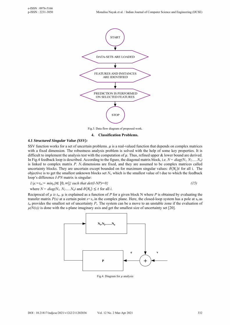
START

DATA-SETS ARE LOADED

FEATURES AND INSTANCESARE IDENTIFIED

PREDICTION IS PERFORMEDON SELECTED FEATURES

STOP

Fig.3. Data flow diagram of proposed work.

4. Classification Problems.

4.1 Structured Singular Value (SSV):

SSV function works for a set of uncertain problems. 𝜇 is a real-valued function that depends on complex matrices with a fixed dimension. The robustness analysis problem is solved with the help of some key properties. It is difficult to implement the analysis test with the computation of 𝜇. Thus, refined upper & lower bound are derived. In Fig.4 feedback loop is described. According to the figure, the diagonal matrix block, i.e. N = diag(N1, N2…..Nn) is linked to complex matrix P. Ni dimensions are fixed, and they are assumed to be complex matrices called uncertainty blocks. They are uncertain except bounded on for maximum singular values: 𝜕 𝑁 𝑡 for all i. The objective is to get the smallest unknown blocks set Ni, which is the smallest value of t due to which the feedback loop’s difference I-PN matrix is singular:

1/µ:=tm:= minp{t∈ 0, ∞ } such that det(I-NP)=0} (15)

where N = diag(N1, N2…..Nn) and 𝜕 𝑁 𝑡 for all i.

Reciprocal of µ is tm. µ is explained as a function of P for a given block N where P is obtained by evaluating the transfer matrix P(s) at a certain point s=so in the complex plane. Here, the closed-loop system has a pole at so as tm provides the smallest set of uncertainty Pi. The system can be a move to an unstable zone if the evaluation of µ(N(s)) is done with the s-plane imaginary axis and get the smallest size of uncertainty set [20].

N1,N2.......Nn

P +

e v

Fig.4. Diagram for 𝜇 analysis



4.2 Rough Set Theory:

An important tool proposed by Professor Pawlak in 1982, i.e. Rough Set Theory [21]. It has two parts. 1st part forms the classification of concepts, relation database, and rules. 2nd part discovers the classification of similarity relation and estimation of the target knowledge. The rough set theory deals with uncertain information where the collection of the membership function is uncertain. In this algorithm, to describe the imprecise concepts, two accurate boundary lines are formed. Here, a decision table is existing where every data are ordered in a table. In this decision table, rows represent the objects and columns represent the features. In a dataset, the class label corresponds to the class that belongs to each row. The class label is represented as decision attributes, and rest are represented as condition attributes where P is the condition attributes and Q is the decision attributes such that P∩Q=𝜑, a ki=ith tuple of the data table. According to equivalent classes introduced by attribute value, this algorithm is divided into three regions, i.e. upper approximation, lower approximation, and boundary. Upper approximation consists of all the objects that are categorized probably. Lower approximation consists of all the items that are being categorized as per the collected data. The boundary contains the objects which are in between lower and upper approximation. Let A= fixed universe of discourse, B= any comparable relation defined on A. (A, B) is called the approximation space consists of let T1, T2, T3……..Tn elements. Assembly of these elements is called a knowledge base. Thus, the upper and lower approximation for any subset M of A is described as:

BM = ∪∈

(16)

𝐵M = ∪∩

(17)

Thus, (BM, 𝐵M) is called a rough set. When M is clear by its approximations, A is distributed into three regions, i.e. negative region NGr(M), boundary region Br(M), and positive region PSR(M).

PSr (M) = BM (18)

NGr (M) = A-𝐵M (19)

Br(M) = 𝐵M-BM (20)

It is trivial that if Br(M) = 𝜑, then B is exact

This method acts as a mathematical tool. Rough sets based methods are defined in [22, 23]. The main benefit of this method is that no added information about the data is needed as in fuzzy set theory, probability in statistics, etc. [24, 25]

5. Feature Selection Algorithm

5.1 The Kruskal-Wallis Test

Kruskal-Wallis is a non-parametric technique that examines the similar behaviour between the samples of the same source from the same circulation or not. In this test, there is a comparison between free samples of dissimilar sample dimensions. The null hypothesis is tested, but if allocations are found dissimilar, then this test withdraws the null hypothesis while the same medians are present [26]. Therefore, the data vectors transfer to the growing order of ranks (R), i.e. T=1 to T=n. In the existence of equal value sequences, there is the assignment of mean ranks. So, the test statistic is described below:

𝐻12

𝑛 𝑛 1𝑘𝑃

3 𝑛 1 (21)

where km = rank sum of mth group

n = ∑ 𝑃 is the sample size.

The Kruskal-Wallis test is defined through an algorithm I.

Algorithm I

Input: l X q matrix, where l is the size of attributes and q is the size of instances

Output: topmost P attributes

To individual attribute fi do i= 1, 2,….l j= 1,2,…….q

a rank Rj is assigned to individual attribute value

rk = ∑ 𝑅∈ is calculated for each class k

using equation(21) the H-value is calculated

the P-value (pi) equivalent to individual H values is calculated by ꭓ2 distribution curve

<i,(𝐻 , 𝑝 )> is emitted

End for



For each attribute 𝑓 do

If 𝑝 <0.001 then

the attribute 𝑓 is selected

Else

the attribute is discarded

End if

End for

<(𝑓 , 𝑓 , …)> is emitted

End

5.2 The Friedman test

Friedman test for equal sample sizes is a non-parametric method for this type of k dependent class. This alternative hypothesis is tested against the null hypothesis, i.e. H(0) = F(1) = F(2)…= F(k). Here the ranking of data vector is in ascending order that ranges from R = 1 to R = M separate for individual classes where M = sample size in the individual class [26]. Statistics of the Friedman test is considered as:

F = ∑ 𝑟 3 𝑚 𝑘 1 (22)

where rl = the rank of lth class

k = class size

Friedman test is discussed in algorithm II

Algorithm II:

Input: l X q matrix where l = size of attributes and q = size of instances


Begin

T individual attribute fi do

the attribute price is divided into their several classes(let M denotes sample size) i= 1,2,……l

rank Rj is assigned to individual feature value of individual class k where j = 1,2,….M

rk = ∑ 𝑅 is calculated for each class

the P-value (pi) equivalent to individual F-value is calculated by ꭓ2 distribution curve

<(Fi,pi)> is emitted

End for

For each attribute fi do

If pi< 0.001 then fsi, the attribute is selected

Else

The attribute is discarded

End if

End for

<(fs1,fs2,…)> is emitted

End

5.3 ANOVA

ANOVA imagines the presence of significant differences among multiple samples means and is valuable in associating the ‘multiple mean’ standards of the dataset [26].

For ANOVA, the statistic is called as F-statistic, and it is calculated by given steps:-

(i) Variation calculation among the group:-

Between Sum of Square(BSS) = 𝑣 𝑌′ 𝑌′ 𝑣 𝑌 𝑌′ ….. (23)

Between Mean Squares(BMS) = BSS/df (24)

(ii) Variation calculation among the group:-

Within Sum of Squares(WSS) = 𝑣 1 𝑝 𝑣 1 𝑝 ….. (25)

Within Mean Squares(WMS) = WSS/𝑑𝑓 (26)

where df = degree of freedom



𝑑𝑓 = (V-n)

p = standard deviation

V= size of sample

n= size of group

𝑉 = sample size in ‘n’ group

(iii) F-test static calculation is described as:

F = BMS/WMS (27)

ANOVA implementation is discussed in algorithm III

Algorithm III

Input: l X q matrix, where l is the size of attributes and q is the size of instances


Begins

For individual attributes 𝑓 do

BMS is calculated with equation (24) i= 1,2……n

WMS is calculated with equation (26)

F-value is calculated (𝐹 𝐵𝑀𝑆/𝑊𝑀𝑆)

the p-value is calculated (𝑝 ) equivalent to individual F-value by the F-distribution curve.

Emit<i,(𝐹 , 𝑝 ) )>

End for

For each attribute 𝑓 do

if 𝑝 <0.001 then

attribute is selected called 𝑓

else

attribute is discarded

end if

end for

emit<(𝑓 , 𝑓 , ….)>

end

6. Results and Discussion

Three kinds of time-series datasets are utilized to estimate the performance of the algorithms. First, feature selection is made from the training data, then the feature selection of significant attributes takes place. Then the significant features are provided to the multilayer perceptron model where the parameters are updated using SMSSO-NN algorithm. The performance comparison of SMSSO-NN is made with and without feature selection methods. The methods are also compared with Rough Set Theory and SSV. The performance of the algorithm is estimated by using the Mean Squared Error (MSE). The MSE can be calculated as:

𝑀𝑆𝐸∑ Y T

N

(28)

where Yn = expected output

T = target

N = total data sample size

The MATLAB software is used for simulation of the results in this section.

6.1 Dataset Details

a) The database consists of a record of absenteeism in office for a duration of three years, i.e. July 2007 to July 2010 at a Brazilian courier company. There are 740 instances and 21 attributes [27]. Training data is taken from July 2007 to July 2009. Prediction is completed for the year July 2010.

b) The second database is the currency exchange rate from INR to USD. The data collection is done from 1st May 2010 to 1stMay 2019. The dataset consists of 2430 rows and six attributes [28]. The training data is from the period of May 2010 to 2018. Testing data is for May 2019.



c) The third data is resulting from blog posts [29]. HTML-documents consists of blog posts that are administered. Prediction is made for all the comments that are from each blog post. Blog posts of previous days are taken as training, and the next day blog posts are taken for testing.

d) The Electricity consumption data [30] is at 10 min intervals for 4.5 months. Humidity and temperature conditions are monitored by the ZigBee wireless sensor network. Previous month Electricity consumption data is taken as training and Electricity consumption of the next day is taken for testing.

Normalization of the data is first done using min-max normalization. The min-max normalization formulae is given by:

𝑋𝑋 𝑋𝑋 𝑋

(29)

6.2 Simulation results

Feature selection algorithms are discussed with SMSSO-NN, SSV and Rough Set Theory in Tables 2, 4, and 6, respectively. The performance of SMSSO-NN, SSV, and Rough Set Theory without feature selection algorithm is discussed in Tables 3, 5, and 7, respectively. The performance of each technique is estimated by MSE value. MSE convergence curve for SMSSO-NN, SSV, and Rough Set Theory for time-series datasets such as absenteeism at work, currency exchange rate, blog feedback dataset, and energy consumption datasets with the use of feature selection algorithm is shown in figure 5, 6, 7, and 8. Comparison of actual versus predicted stock values for SMSSO-NN, SSV, and Rough Set Theory for absenteeism at work dataset with feature selection methods such as ANOVA, Friedman test and Kruskal-Walis is shown in figure 9, 13 and 17. Comparison of actual versus predicted stock values for SMSSO-NN, SSV, and Rough Set Theory for the currency exchange rate dataset with algorithms of feature selection is shown in figure 12, 16 and 20 respectively. Comparison of actual versus predicted stock values for SMSSO-NN, SSV, and Rough Set Theory for blog feedback dataset with algorithms of feature selection is shown in figure 10, 14 and 18 respectively. Comparison of actual versus predicted stock values for SMSSO-NN, SSV, and Rough Set Theory for electricity consumption dataset with algorithms of feature selection is shown in figure 11, 15, and 19 respectively.

Table-1: Relevant features

Datasets No. of samples No. of features Feature selection methods No. of features selected

Absenteeism at work

740 21 ANOVA 14

KRUSKAL-WALIS 15

FRIEDMAN TEST 13

Currency Exchange

2430 6 ANOVA 5

KRUSKAL-WALIS 4

FRIEDMAN TEST 5

Blog feedback

data

52397 281 ANOVA 201

KRUSKAL-WALIS 204

FRIEDMAN TEST 210

Electricity Consumption

19736 29 ANOVA 20

KRUSKAL-WALIS 18

FRIEDMAN TEST 16

Table 1 describes each dataset in a detailed manner with the important features selected from each of the feature selection algorithms.



Table 2: Particulars of each method with feature selection while testing in SMSSO-NN

Feature selection method

Datasets Time (in seconds) MSE value

Training time Testing time

ANOVA Absenteeism at work 3.431 1.232 0.615

Currency exchange rate 1.142 1.341 0.542

Blog feedback Data 3.112 1.302 0.812

Electricity Consumption 2.321 1.452 0.862

KRUSKAL WALIS

Absenteeism at work 2.821 1.403 0.731

Currency exchange 1.801 1.471 0.723



FRIEDMAN TEST





Table 3: Particulars of each datasets while testing without using any feature selection method in SMSSO-NN

Datasets Training Time (in seconds) Testing time in seconds MSE





Table 4: Particulars of each methods while testing with feature selection in SSV

Feature selection Technique

Datasets Training Time (in seconds)

Testing time (in seconds)

MSE




Energy Consumption 2.342 1.328 1.112

KRUSKAL WALIS Absenteeism at work 2.809 1.352 0.923




FRIEDMAN TEST Absenteeism at work 3.423 1.206 1.614




Table 5: Particulars of each datasets while testing without any feature selection in SSV

Datasets Training Time(in seconds) Testing Time (in seconds) MSE



Blog feedback Data 2.731 1. 425 0.741




Table 6: Particulars of each method while testing with feature selection in Rough Set Theory

Feature selection Technique

Datasets Training Time (in seconds)

Testing time (in seconds)

MSE





KRUSKAL WALIS Absenteeism at work 2.809 1.352 0.923




FRIEDMAN TEST Absenteeism at work 3.423 1.206 1.614




Table 7: Particulars of each datasets while testing without any feature selection in Rough Set Theory

Datasets Training Time (in Seconds) Testing Time (in Seconds) MSE





Fig. 5 MSE convergence of absenteeism at work



Fig.6 MSE convergence of currency exchange rate

Fig.7 MSE convergence of blog feedback data



Fig.8 MSE convergence of electricity consumption

Fig 9 Assessment of Absenteeism value using ANOVA



Fig10. Assessment of blog feedback using ANOVA

Fig 11. Assessment of electricity consumption using ANOVA



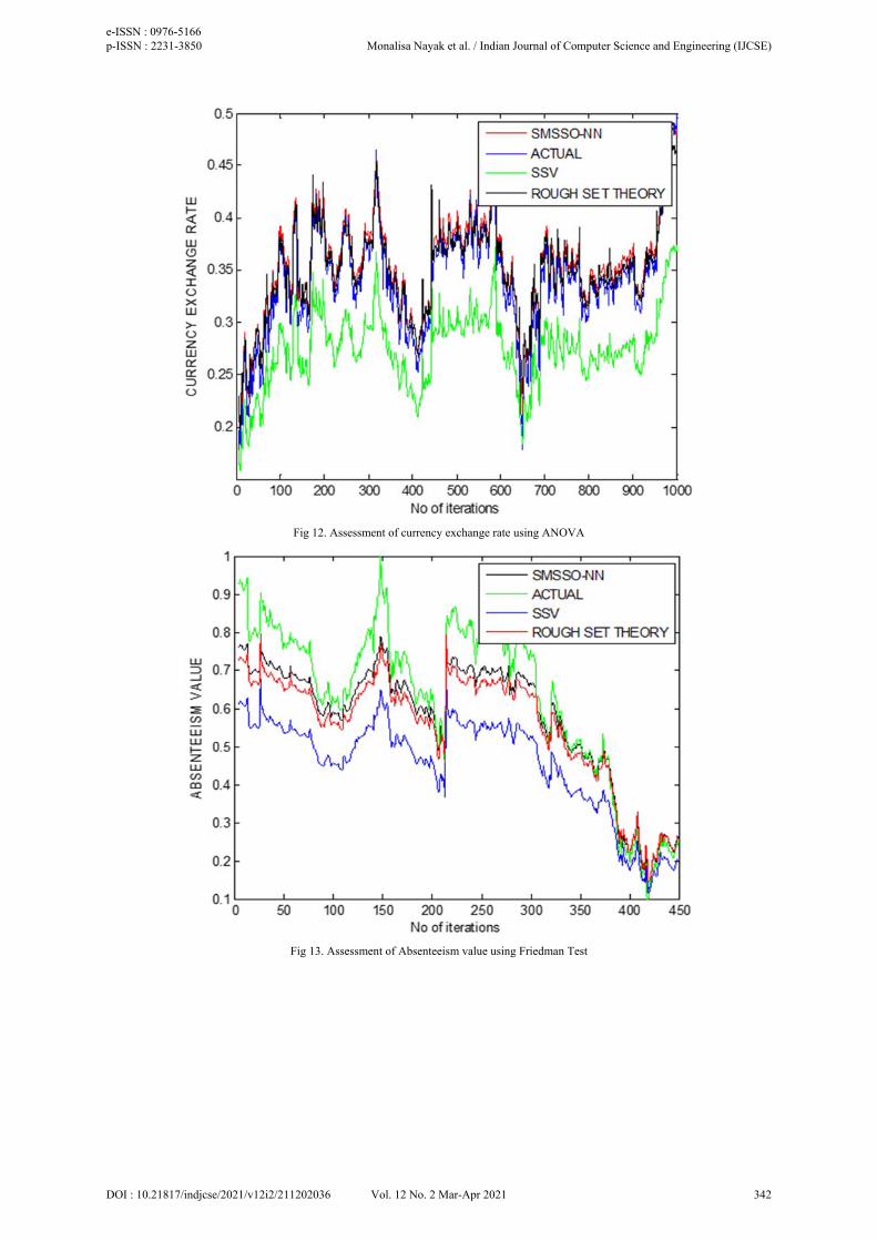
Fig 12. Assessment of currency exchange rate using ANOVA

Fig 13. Assessment of Absenteeism value using Friedman Test



Fig 14. Assessment of blog feedback data using Friedman Test

Fig 15. Assessment of electricity consumption using Friedman Test



Fig 16. Assessment of electricity consumption using Friedman Test

Fig 17. Assessment of Absenteeism value using Kruskal-Wallis



Fig 18. Assessment of Blog feedback data using Kruskal-Wallis

Fig 19. Assessment of Electricity Consumption using Kruskal-Wallis



Fig 20. Assessment of currency exchange rate using Kruskal-Wallis

7. Conclusion

Financial time-series data varies with time and is noisy by nature. It's been a challenging task for researchers to predict the time-series data effectively because of the irregular patterns present within datasets. Traditional methods fail to analyse the time-series data correctly due to their chaotic and volatile behaviour of time-series data.

In this paper, analysis of four different types of financial time-series datasets, i.e. absenteeism at work, currency exchange rate, blog feedback dataset, and energy consumption are considered with and without feature selection. Three feature selection techniques are used, i.e. ANOVA, Kruskal Walis, and Friedman test. Feature selection significantly reduces the size of the dataset, which provides better study. The performance of the methods is examined using MSE value. The SMSSO-NN technique shows minimum MSE of 0.542 in 1.142 sec of testing time with ANOVA in currency exchange rate, 0.613 in 1.112 sec of testing time with Kruskal Walis in blog feedback data, and 0.403 in 1.367 sec with Friedman test using electricity consumption dataset which is better than other classification algorithms like Rough Set Theory and Structured Singular value. Moreover, SMSSO-NN shows minimum MSE of 0.210 in 2.102 sec without feature selection in the blog feedback dataset. In the future, larger datasets can be used in evaluating the performance of SMSSO-NN algorithm.

References [1] Reid D, Hussain A.J and Tawfik H, “Financial Time-series Prediction Using Spiking Neural Networks”, PLOS one, 9(8)

(2014)10.1371/journal.pone.0103656 [2] Ravi V, Dadabada P.K, Deb K, “Financial time-series prediction using hybrids of chaos theory, multi-layer perceptron and multi-

objective evolutionary algorithms”, Swarm and Evolutionary Computation,36, 136–149 (2017) http://dx.doi.org/10.1016/j.swevo.2017.05.003

[3] LiaoJ.J et al, “An ensemble-based model for two-class imbalanced financial problem”, Economic Modelling,37, 175-183(2014)https://doi.org/10.1016/j.econmod.2013.11.013

[4] Badea L.M (Stroie), “Predicting Consumer Behaviour with Artificial Neural Networks”, Procedia Economics and Finance, 15,238-246 (2014), https://doi.org/10.1016/S2212-5671(14)00492-4

[5] Zhao Z et al, “Investigation and improvement of multi-layer perceptron neural networks for credit scoring”, Expert Systems with Applications,42(7), 3508-3516(2015)https://doi.org/10.1016/j.eswa.2014.12.006

[6] ZhouT et al, “Financial time-series prediction using a dendritic neuron model”, Knowledge-Based Systems, 105, 214-224(2016)https://doi.org/10.1016/j.knosys.2016.05.031

[7] Rout A.K et al,“Forecasting financial time-series using a low complexity recurrent neural network and evolutionary learning approach”, Journal of King Saud University - Computer and Information Sciences, 29(4),536-552(2017) https://doi.org/10.1016/j.jksuci.2015.06.002

[8] Dadabada P.K and Ravi V, “Forecasting financial time-series volatility using Particle Swarm Optimization trained Quantile Regression Neural Network”, Applied Soft Comp, 58, 35-52(2017) https://doi.org/10.1016/j.asoc.2017.04.014

[9] Zhou Y et al. “A Simplex method-based social spider optimization algorithms for clustering analysis”, Engineering Applications of Artificial Intelligence, 64, 67-82 (2017).

[10] Cuevas E, Cienfuegos M. "A new algorithm inspired in the behavior of the social spider for constrained optimization". Expert Syst. Appl. Elsevier, 41(2), 412–425(2014)10.1016/j.eswa.2013.07.067



[11] Cuevas E, Cienfuegos M, Zaldívar, D, Pérez-Cisneros M, “A swarm optimization algorithm inspired in the behavior of the social-spider”, Expert Syst. Appl. 40(16), 6374–6384(2013) 10.1016/j.eswa.2013.05.041

[12] Aviles L, “Causes and consequences of cooperation and permanent-sociality in spiders”, In Choe, B.C. (Ed.). The evolution of social behavior in insects and arachnids. Cambridge University Press, Cambridge, MA, 476–498(1997).

[13] Yip C, Eric K.S, “Cooperative capture of large prey solves scaling challenge faced by spider societies”. Proc.Natl.Acad.Sci.USA,105(33), 11818–11822(2008)10.1073/pnas.0710603105

[14] Rayor E.C, “Do social spiders cooperate in predator defense and foraging without a web?” Behav. Ecol. Sociobiol, 65(10), 1935–1945(2011) 10.1007/s00265-011-1203-5

[15] Aviles L, “Sex-ratio bias and possible group selection in the social spider anelosimus eximius”, UniversityofChicago, PressJ,128(1),1–12(1986). https://www.jstor.org/stable/2461281

[16] Spendley W.G.R.F.R, Hext G.R., Himsworth F.R, “Sequential application of simplex designs in optimization and evolutionary operation”, Taylor & Francis, 4(4), 441–461(1962), 10.2307/1266283

[17] Nelder J.A, Mead R,“A Simplex method for function minimization”, Comput. J. 30, 8–313(1965) 10.1093/comjnl/7.4.308 [18] Yen J, Lee B, “A simplex genetic algorithm hybrid”. Evolutionary Computation, IEEE Conf.175–180(1997)10.1109/ICEC.1997.592291 [19] Storn R, Price K,“Differential evolution – a simple and efficient heuristic for global optimization over continuous spaces”. J. Global

Optim. 11, 341–359(1997)10.1023/A:1008202821328 [20] Daily R.L, “A new algorithm for the real structured singular value”, American control conf. (1990) 10.23919/ACC.1990.4791276 [21] Bagyamathi, M.; Inbarani, H.H.: A novel hybridized rough set and improved harmony search based feature selection for protein

sequence classification, Big Data in Complex Sys. 9, 173-204(2015). 10.1007/978-3-319-11056-1_6 [22] RSES: Rough Set Exploration System. http://logic.mimuw.edu.pl/rses/. [23] The ROSETTA, homepage Norwegian University of Science and Technology, Department of Computer and Information Science.

NTNU.http://www.idi.ntnu.no/aleks/rosetta/ [24] Thangavel, K.; Pethalakshmi, A.: Dimensionality reduction based on rough set theory: a review, Applied Soft Computing, 9, 1-12(2009).

10.1016/j.asoc.2008.05.006 [25] Inbarani, H.H.; Bagyamathi, M.; Azar, A.T.: A novel hybrid feature selection method based on rough set and improved harmony search,

Neural Comput. & Applic. 26, 1859–1880(2015). 10.1007/s00521-015-1840-0 [26] Kumar M and Rath S.K, “Classification of Microarray using MapReduce based Proximal Support Vector Machine Classifier”,

Knowledge-Based Systems (2015) http://dx.doi.org/10.1016/j.knosys.2015.09.005 [27] Martiniano, A., Ferreira, R. P., Sassi, R. J., & Affonso, C. “Application of a neuro-fuzzy network in the prediction of absenteeism at

work”. In Information Systems and Technologies (CISTI), 7th Iberian Conference on IEEE, pp. 1-4, (2012). [28] www. Investing.com [29] Buza, K. (2014). “Feedback Prediction for Blogs. In Data Analysis, Machine Learning and Knowledge Discovery” (pp. 145-152).

Springer International Publishing.https://doi.org/10.1007/978-3-319-01595-8_16 [30] Luis M. Candanedo, Veronique Feldheim, and Dominique Deramaix, “Data-driven prediction models of energy use of appliances in a

low-energy house”, Energy and Buildings, 140, 81-97, (2017) ISSN 0378-7788. https://doi.org/10.1016/j.enbuild.2017.01.083



FINANCIAL TIME-SERIES PREDICTION WITH FEATURE …

Documents

Transcript of FINANCIAL TIME-SERIES PREDICTION WITH FEATURE …