
Financial stress transmission in EMU sovereign bond … · Financial stress transmission in EMU...
36
1 DOCUMENTOS DE ECONOMÍA Y FINANZAS INTERNACIONALES Working Papers on International Economics and Finance DEFI 15-02 February 2015 Financial stress transmission in EMU sovereign bond market volatility: a connectedness analysis. Fernando Fernández-Rodríguez Marta Gómez-Puig Simón Sosvilla-Rivero Asociación Española de Economía y Finanzas Internacionales www.aeefi.com ISSN: 1696-6376
Transcript of Financial stress transmission in EMU sovereign bond … · Financial stress transmission in EMU...
1
DOCUMENTOS DE ECONOMÍA Y FINANZAS INTERNACIONALES
Working Papers on International
Economics and Finance
DEFI 15-02
February 2015
Financial stress transmission in EMU sovereign bond market
volatility: a connectedness analysis.
Fernando Fernández-Rodríguez
Marta Gómez-Puig
Simón Sosvilla-Rivero
Asociación Española de Economía y Finanzas Internacionales www.aeefi.com ISSN: 1696-6376
2
Financial stress transmission in EMU sovereign bond market volatility: a connectedness analysis.
Fernando Fernández-Rodrígueza, Marta Gómez-Puigb and Simón Sosvilla-Riveroc* aDepartment of Quantitative Methods in Economics, Universidad de Las Palmas de
Gran Canaria, 35017 Las Palmas de Gran Canaria, Spain
bDepartment of Economic Theory, Universitat de Barcelona. 08034 Barcelona, Spain
cComplutense Institute of International Studies, Universidad Complutense de Madrid. 28223 Madrid, Spain
January 2015
Abstract
This paper measures the connectedness in EMU sovereign market volatility between
April 1999 and January 2014, in order to monitor stress transmission and to identify
episodes of intensive spillovers from one country to the others. To this end, we first
perform a static and dynamic analysis to measure the total volatility connectedness in
the entire period (the system-wide approach) using a framework recently proposed by
Diebold and Yılmaz (2014). Second, we make use of a dynamic analysis to evaluate the
net directional connectedness for each country and apply panel model techniques to
investigate its determinants. Finally, to gain further insights, we examine the time-
varying behaviour of net pair-wise directional connectedness at different stages of the
recent sovereign debt crisis.
Keywords: Sovereign debt crisis, Euro area, Market Linkages, Vector Autoregression,
Variance Decomposition.
JEL Classification Codes: C53, E44, F36, G15
*Corresponding author. Tel.: +34 913942342; fax: +34 913942591.
E-mail addresses: [email protected] (F. Fernández-Rodríguez), [email protected] (M. Gómez-Puig), [email protected] (S. Sosvilla-Rivero)
3
1. Introduction
Regulatory convergence and the elimination of currency risk1 are two of the reasons
behind the significant increase in cross-border financial activity in the euro area since
the beginning of the twenty-first century (see Kalemli-Ozcan et al., 2009 and Barnes et
al., 2010). This effect has been even stronger in some of the EMU peripheral countries2.
However, although cross-border banking clearly benefits risk diversification in
businesses’ portfolios and is considered by monetary authorities as a hallmark of
successful financial integration, it also presents some drawbacks. First, foreign capital is
likely to be much more mobile than domestic capital; in a crisis situation, foreign banks
may simply decide to “cut and run”. Moreover, in an integrated banking system,
financial or sovereign crises in a country can quickly spill over into other countries.
Indeed, given the high degree of interconnectedness in European financial markets, a
major fear was that the default of the sovereign/banking sector in one EMU country
could have spillover effects that might result in subsequent defaults in the euro area as a
whole (see Schoenmaker and Wagner, 2013)3.
In this context, an important reason and justification for providing financial support to
Greece in May 2010 was precisely the “fear” of contagion (see, for instance,
Constâncio, 2012), not only because there was a sudden loss of confidence among
investors, who turned their attention to the macroeconomic and fiscal imbalances within
EMU countries which had largely been ignored until then (see Beirne and Fratzscher,
2013), but also because several European Union banks had a particularly high exposure
to Greece (see Gómez-Puig and Sosvilla-Rivero, 2013).
Indeed, from late 2009 onwards, the demand for the German bund grew due its safe
haven status, and yield spreads of euro area issues with respect to Germany spiralled
(see Figure 1). Besides, since May 2010, not only has Greece been rescued twice, but
Ireland, Portugal and Cyprus also needed bailouts to stay afloat.
[Insert Figure 1 here]
1 The introduction of the Single Banking License in 1989 through the Second Banking Directive was a decisive step towards a unified European financial market, which subsequently led to a convergence in financial legislation and regulation across member countries. 2 In particular, the sources of external financing for Portuguese and Greek banks radically shifted on joining the euro; traditionally reliant on dollar debt, their banks were subsequently able to raise funds from their counterparts elsewhere in the EMU (See Spiegel, 2009a and 2009b) 3 Theoretical research modelling various aspects of the costs and benefits of cross-border banking (e.g. Dasgupta 2004; Goldstein and Pauzner 2004;Wagner 2010) concludes that some degree of integration is beneficial but that an excessive degree may not be.
4
In this scenario, where we have seen how crisis episodes in a given EMU sovereign
market affect other markets almost instantaneously, some important questions have
emerged that economists, policymakers, and practitioners need to address urgently. To
what extent was the sovereign risk premium increase in the euro area during the
European sovereign debt crisis due only to deteriorated debt sustainability in member
countries? Did markets’ degree of connectedness play any significant role in this
increase?
Researchers have already studied transmission and/or contagion between sovereigns in
the euro area context using a variety of methodologies (correlation-based measures,
conditional value-at-risk (CoVaR), or Granger-causality approach, among others)4:
Kalbaska and Gatkowski (2012), Metiu (2012), Caporin et al. (2013), Beirne and
Fratzscher (2013), Gorea and Radev (2014), Gómez-Puig and Sosvilla-Rivero (2014) or
Ludwig (2014) to name a few.
Nevertheless, in this paper we will focus on the interconnection between EMU
sovereign debt markets by applying a methodology which has not been widely used in
this area. Specifically, we will make use of Diebold and Yilmaz (2014)’s measures of
connectedness (both system-wide and pair-wise) in order to contribute to the literature
on international transmission mechanisms that the sovereign debt crisis in the euro area
has rekindled, and to be able to answer some of the previously posed questions.
This literature includes two groups of theories which, though not necessarily mutually
exclusive (see Dungey and Gajurel, 2013), have fostered considerable debate. On the
one hand, since fundamentals of different countries may be interconnected by their
cross-border flows of goods, services, and capital, or common shocks may adversely
affect several economies simultaneously, transmission between countries may occur.
These effects are known in the literature as “spillovers” (Masson, 1999),
“interdependence” (Forbes and Rigobon, 2002), or “fundamentals-based contagion”
(Kaminsky and Reinhart, 2000). On the other hand, financial crises in one country may
conceivably trigger crises elsewhere for reasons unexplained by macroeconomic
fundamentals – perhaps because they lead to shifts in market sentiment, change the
interpretation given to existing information, or trigger herding behaviour. This
transmission mechanism is known in the literature as “pure contagion” (Masson, 1999).
In this context, the measures of connectedness proposed by Diebold and Yilmaz (2014)
4 See Biblio et al. (2012) for a review of the measures proposed in the literature to estimate those linkages.
5
can be considered as a bridge between the two visions mentioned above, since they
examine volatility spillovers using useful information on agents’ expectations5, and
sidestep the contentious issues associated with the definition and existence of episodes
of “fundamentals-based” or “pure” contagion.
A substantial amount of literature uses different extensions of Diebold and Yilmaz
(2012)’s previous methodology to examine spillovers and transmission effects in stock,
foreign exchange, or oil markets in non-EMU countries. Awartania et al. (2013), Lee
and Chang (2013), Chau and Deesomsak (2014) and Cronin (2014) apply this
methodology to examine spillovers in the United States’ markets; Yilmaz (2010), Zhou
et al. (2012) or Narayan et al. (2014) focus on Asian countries; Apostolakisa and
Papadopoulos (2014) and Tsai (2014) examine G-7 economies, and Duncan and
Kabundi (2013) centre their analysis on South African markets. However, few papers to
date have looked at the connectedness and spillover effects within euro area sovereign
debt markets, even though quantifying the spillover risk is a very important tool in order
to assess whether the benefits of a sovereign bailout may outweigh its costs.
Some exceptions are Antonakakis and Vergos (2013), who examined spillovers between
10 euro area government yield spreads during the period 2007-2012; Claeys and
Vašicek (2014), who examined linkages between 16 European sovereign bond spreads
during the period 2000-2012; Glover and Richards-Shubik (2014), who applied a model
based on the literature on contagion in financial networks to data on sovereign credit
default swap spreads (CDS) among 13 European sovereigns from 2005 to 2011; and
Alter and Beyer (2014), who quantify spillovers between sovereign credit markets and
banks in the euro area. While the above authors apply Diebold and Yilmaz’s
methodology, Favero (2013) proposes an extension to Global Vector Autoregressive
(GVAR) models to capture time-varying interdependence between EMU sovereign
yield spreads.
However, to our knowledge, no empirical analyses have been performed of the
connectedness in sovereigns’ market volatility, in spite of its profound importance. As
volatility reflects the extent to which the market evaluates and assimilates the arrival of
new information, the analysis of its pattern of transmission may provide insights into
the characteristics and dynamics of sovereign debt markets. This information might help
5 Since uncertainty is based on how much of the forecasting error variance cannot be explained by shocks in the variable, expectations gauge the evolution of both fundamental and market sentiment variables.
6
to obtain a better understanding of yield evolution over time, providing a barometer for
the vulnerability of these markets.
Moreover, since volatility tracks investor fear, by measuring and analyzing the dynamic
connectedness in volatility we are able to examine the “fear of connectedness”
expressed by market participants as they trade. So, given that volatility tracks investors’
perceived risk and is a crisis-sensitive variable which can induce “volatility surprise”
(Engle 1993), this paper centres on the analysis of connectedness in EMU sovereign
debt market volatility using Diebold and Yilmaz (2014)’s methodology in order to fill
the existing gap in the literature.
Moreover, Diebold and Yilmaz (2014) showed that the connectedness framework was
closely linked with both modern network theory (see Glover and Richards-Shubik,
2014) and modern measures of systemic risk (see Ang and Longstaff, 2013 or
Acemoglu et al., 2014). The degree of connectedness, on the other hand, measures the
contribution of individual units to systemic network events, in a fashion very similar to
the CoVaR of this unit (see, e. g., Adrian and Brunnermeier, 2008).
This paper explores this challenging avenue of research, focusing our study on
connectedness in EMU sovereign bond market volatility during the period from April
1999 to January 2014. However, unlike previous studies, in the analysis we will only
include euro area countries and work with 10-year yields instead of spreads over the
German bund, in order to be able to include Germany in the study.
After explaining the methodology that will be used in the empirical analysis, we will
proceed in four stages. First, in order to estimate system-wide connectedness, we will
undertake a full-sample (static analysis) that is not only of intrinsic interest, but will also
prepare the way for the second stage: the performance of a dynamic (rolling-sample)
analysis of conditional connectedness. In the third stage, we will “zoom in” on the
evolution of net directional connectedness in each market and assess whether their
determinants differ between EMU central and peripheral countries. Finally, in the last
stage we will examine how net pair-wise connectedness changes over the sample
period.
Overall, our results suggest that the positive influence exerted by economically sound
core countries over peripheral ones in the stability period suddenly vanished with the
outbreak of the crisis, when investors disavowed the shelter that peripheral countries
7
could find in central countries and turned their attention to the major imbalances that
they presented. Consequently, during the period of stability, beside the slight
differences in yield behaviour (all followed the evolution of the German bund, and
spreads moved in a very narrow range) it was the central countries that triggered net
connectedness relationships; in the crisis period, however, there was a major shift and
this role was now played by peripheral countries. Therefore, according to our results, in
a context of increased cross-border financial activity in the euro-area, the concern that in
turbulent times a shock in one country might have spillover effects into others may be
well founded, and global financial stability may be threatened.
The rest of the paper is organized as follows. Section 2 presents Diebold and Yılmaz
(2014)’s methodology for assessing connectedness in financial market volatility, and the
empirical results (both static and dynamic) obtained for our sample of EMU sovereign
markets (a system-wide measure of connectedness). In Section 3 we present the
empirical results regarding the evolution of net directional connectedness in each
market, and explore its determinants. Section 4 examines the time-varying behaviour of
net pair-wise directional connectedness at different stages of the current financial crisis.
Finally, Section 5 summarizes the findings and offers some concluding remarks.
2. Connectedness analysis
2.1. Econometric methodology
The main tool for measuring the amount of connectedness is based on a decomposition
of the forecast error variance, which we will now briefly describe.
Given a multivariate empirical time series, the forecast error variance decomposition
results from the following steps:
1. Fit a standard vector autoregressive (VAR) model to the series.
2. Using series data up to and including time t, establish an H period-ahead forecast (up
to time t + H).
3. Decompose the error variance of the forecast for each component with respect to
shocks from the same or other components at time t.
Diebold and Yilmaz (2014) propose several connectedness measures built from pieces
of variance decompositions in which the forecast error variance of variable i is
8
decomposed into parts attributed to the various variables in the system. This section
provides a summary of their connectedness index methodology.
Let us denote by dHij the ij-th H-step variance decomposition component (i.e., the
fraction of variable i’s H-step forecast error variance due to shocks in variable j). The
connectedness measures are based on the “non-own”, or “cross”, variance
decompositions, dHij, i, j = 1, . . . , N, i ≠ j.
Consider an N-dimensional covariance-stationary data-generating process (DGP) with
orthogonal shocks: ,)( tt uLx ...,)( 2210 LLL .),( IuuE tt Note that
0 need not be diagonal. All aspects of connectedness are contained in this very general
representation. Contemporaneous aspects of connectedness are summarized in 0 and
dynamic aspects in ,...}.,{ 21 Transformation of ,...},{ 21 via variance
decompositions is needed to reveal and compactly summarize connectedness. Diebold
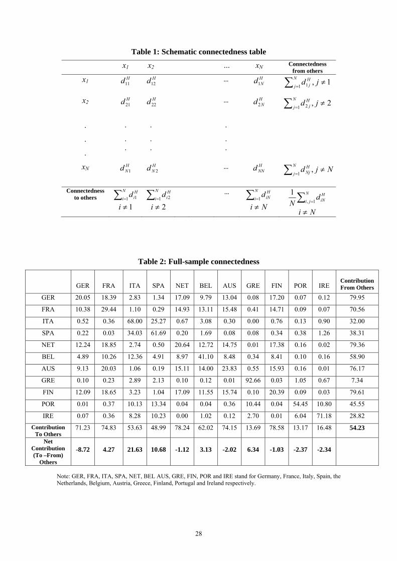
and Yilmaz (2014) propose a connectedness table such as Table 1 to understand the
various connectedness measures and their relationships. Its main upper-left NxN block,
which contains the variance decompositions, is called the “variance decomposition
matrix," and is denoted by ].[ ijH dD The connectedness table increases HD with a
rightmost column containing row sums, a bottom row containing column sums, and a
bottom-right element containing the grand average, in all cases for i ≠ j.
[Insert Table 1 here]
The off-diagonal entries of HD are the parts of the N forecast-error variance
decompositions of relevance from a connectedness perspective. In particular, the gross
pair-wise directional connectedness from j to i is defined as follows:
.Hij
Hji dC
Since in general ,Hij
Hji CC the net pair-wise directional connectedness from j to i,
can be defined as:
.Hji
Hij
Hij CCC
As for the off-diagonal row sums in Table 1, they give the share of the H-step forecast-
error variance of variable xi coming from shocks arising in other variables (all others, as
opposed to a single other), while the off-diagonal column sums provide the share of the
9
H-step forecast-error variance of variable xi going to shocks arising in other variables.
Hence, the off-diagonal row and column sums, labelled “from" and “to" in the
connectedness table, offer the total directional connectedness measures. In particular,
total directional connectedness from others to i is defined as
,1
N
ijj
Hij
Hi dC
and total directional connectedness to others from i is defined as
.1
N
ijj
Hji
Hi dC
We can also define net total directional connectedness as
. Hi
Hi
Hi CCC
Finally, the grand total of the off-diagonal entries in DH (equivalently, the sum of the
“from" column or “to" row) measures total connectedness:
.1
1,
N
ijji
Hij
H dN
C
For the case of non-orthogonal shocks, the variance decompositions are not as easily
calculated as before, because the variance of a weighted sum is not an appropriate sum
of variances; in this case, methodologies for providing orthogonal innovations like
traditional Cholesky-factor identification may be sensitive to ordering. So, following
Diebold and Yilmaz (2014), a generalized VAR decomposition (GVD), invariant to
ordering, proposed by Koop et al. (1996) and Pesaran and Shin (1998) will be used. The
H-step generalized variance decomposition matrix is defined as gH gHijD d , where
1 21
01
0
´
´ ´
H
jj i h jgH hij H
i h h jh
e ed
e e
In this case, je is a vector with jth element unity and zeros elsewhere, h is the
coefficient matrix in the infinite moving-average representation from VAR, is the
covariance matrix of the shock vector in the non-orthogonalized-VAR, jj being its jth
10
diagonal element. In this GVD framework, the lack of orthogonality means that the
rows of gHijd do not have sum unity and, in order to obtain a generalized connectedness
index g gijD d , the following normalization is necessary:
1
gijg
ij Ngij
j
dd
d
, where by
construction 1
1N
gij
j
d
and , 1
Ngij
i j
d N
The matrix g gijD d permits us to define similar concepts as defined before for the
orthogonal case, that is, total directional connectedness, net total directional
connectedness, and total connectedness.
2.2. Data
We use daily data of 10-year bond yield volatility built on data collected from the
Thomson Reuters Datastream for eleven EMU countries: both central (Austria,
Belgium, Finland, France, Germany and the Netherlands) and peripheral countries
(Greece, Ireland, Italy, Portugal and Spain). Our sample begins on 1 April 1999 and
ends on 27 January 2014 (i.e., a total of 3,868 observations)6, spanning several
important financial market episodes in addition to the crisis of 2007-2008 – in
particular, the euro area sovereign debt crisis from 2009 onwards.
2.3. Static (full-sample, unconditional) analysis
The full-sample connectedness table appears as Table 2. As mentioned above, the ijth
entry of the upper-left 11x11 country submatrix gives the estimated ijth pair-wise
directional connectedness contribution to the forecast error variance of country i’s
volatility yields coming from innovations to country j. Hence, the off-diagonal column
sums (labelled TO) and row sums (labelled FROM) gives the total directional
connectedness to all others from i and from all others to i respectively. The bottom-most
row (labelled NET) gives the difference in total directional connectedness (to-from).
Finally, the bottom-right element (in boldface) is total connectedness.
6 The sample starts in April 1999 since data for Greece are only available from that date onwards.
11
[Insert Table 2 here]
As can be seen, the diagonal elements (own connectedness) are the largest individual
elements in the table, but total directional connectedness (from others or to others) tends
to be much larger, except for the EMU peripheral countries. In addition, the spread of
the “from” degree distribution is noticeably greater than that of the “to” degree
distribution for six out of the eleven cases under study.
Regarding pair-wise directional connectedness (the off-diagonal elements of the upper-
left 11 × 11 submatrix), the highest observed pair-wise connectedness is from Italy to
Spain (34.03%). In return, the pair-wise connectedness from Spain to Italy (25.27%) is
the second-highest. The highest value of pair-wise directional connectedness between
EMU central countries is from France to Austria (20.03%), followed by that from
France to the Netherlands (18.85%). The total directional connectedness from others,
which measures the share of volatility shocks received from other bond yields in the
total variance of the forecast error for each bond yield, ranges between 7.34% (Greece)
and 79.95% (Germany). As for the total directional connectedness to others, our results
suggest that it varies from a low of 13.17% for Greece to 78.58% for Finland: a range of
65.41 points for connectedness to others, lower than the range of 72.61 points found for
connectedness from others. Finally, we obtain a value of 54.23% for the total
connectedness between the eleven countries under study for the full sample (system-
wide measure) – significantly lower than the value of 78.3% obtained by Diebold and
Yilmaz (2014) for US financial institutions, or the 97.2% found by Diebold and Yilmaz
(2012) for international financial markets.
2.4 Dynamic (rolling, conditional) analysis
The full-sample connectedness analysis provides a good characterization of
“unconditional” aspects of the connectedness measures. However, it does not help us to
understand the connectedness dynamics. The appeal of connectedness methodology lies
in its use as a measure of how quickly return or volatility shocks spread across countries
as well as within a country. This section presents an analysis of dynamic connectedness
which relies on rolling estimation windows.
The dynamic connectedness analysis starts with total connectedness, and then moves on
to net directional connectedness across countries in Section 3.
12
2.4.1. Total connectedness
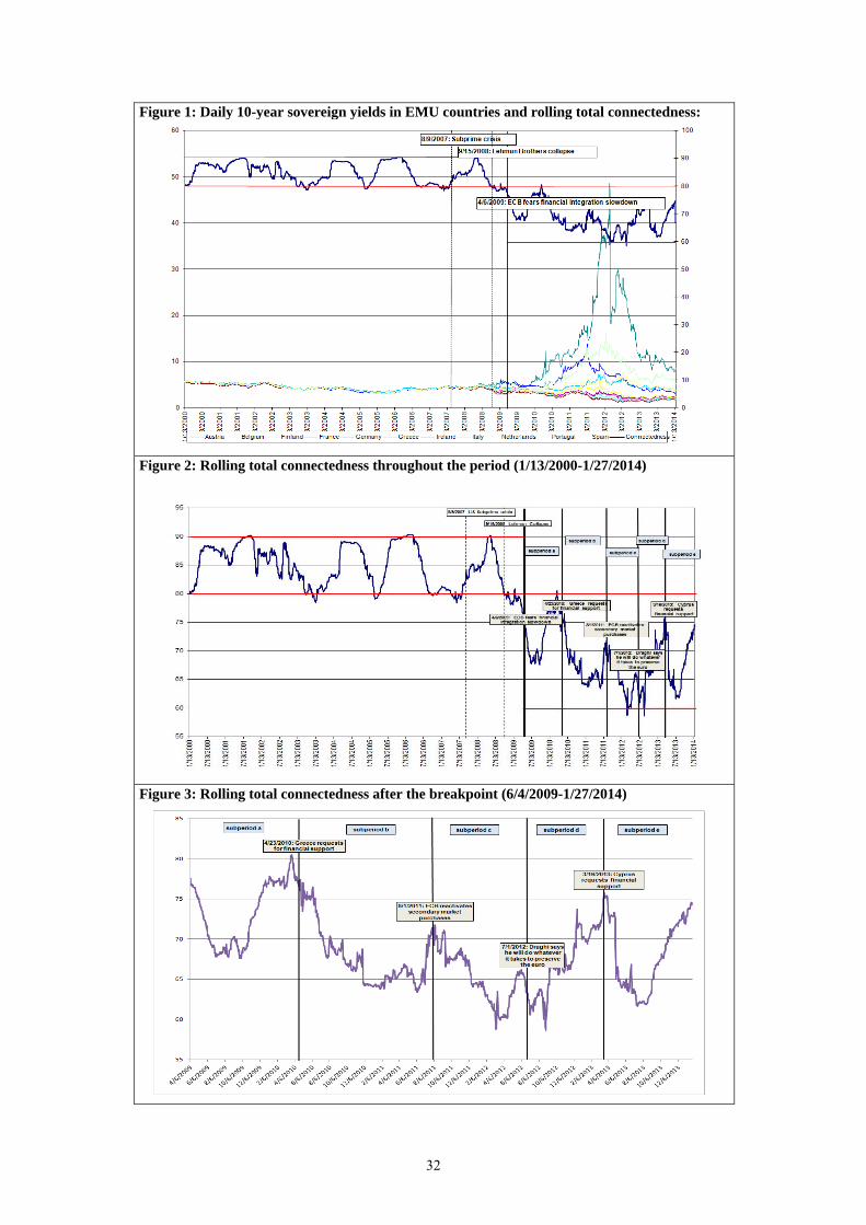
In Figures 1 to 3 we plot total volatility connectedness over 200-day rolling-sample
windows and using 10 days as the predictive horizon for the underlying variance
decomposition. In Figure 1 the rolling total connectedness is plotted along with the
evolution of daily 10-year sovereign yields, while in Figures 2 and 3 it is plotted
separately.
In Figure 1, we can identify two distinct periods in the evolution of the total level of
connectedness, which coincide with the evolution of 10-year yields. In the first period
(which we will term the “stability period”), the level of connectedness of the EMU
sovereign debt market is high, matching the close evolution of 10-year yields (the
spreads moved in a narrow range and reached values close to zero). Neither the US
subprime crisis of August 2007 nor the Lehman Brothers Collapse of September 2008
seemed to have a substantial effect on, euro area sovereign debt markets and their high
level of connectedness.
However, in April 2009, coinciding with a statement by the European Central Bank
(ECB) expressing its fears of a slowdown in financial market integration, and only some
months before Papandreou’s government announced Greece’s distressed debt position
(November 2009)7, sovereign yields begin to spiral and total connectedness began a
downturn trend. From then on, in parallel with the increase in sovereign yields,
connectedness decreased and entered a different regime. These results are in
concordance with Gómez-Puig and Sosvilla-Rivero (2014) who, by applying the
Quandt–Andrews and Bai and Perron tests (1998, 2003), allowed the data to select
when regime shifts occur in each potential causal relationship. Their results suggest that
69 out of the 110 breakpoints (i.e., 63%) occurred after November 2009, after
Papandreou’s government had revealed that its finances were far worse than previously
announced.
[Insert Figure 2 here]
7 In November 2009, Papandreou’s government disclosed that its financial situation was far worse than it had previously announced, with a yearly deficit of 12.7% of GDP – four times more than the euro area’s limit, and more than double the previously published figure – and a public debt of $410 billion. We should recall that this announcement only served to worsen the severe crisis in the Greek economy; the country’s debt rating was lowered to BBB+ (the lowest in the euro zone) on 8 December. These episodes marked the beginning of the euro area’s sovereign debt crisis.
13
Moreover, the existence of two different regimes in the evolution of connectedness8 and
the abrupt decrease in the mean in the second regime may explain the low value
(54.23%) obtained for the total connectedness (system-wide measure) between the
eleven countries studied over the full period. Therefore, since the second regime
coincides with the euro area sovereign debt crisis, we will focus our analysis on this
period (denoted as the crisis period and spanning from April 2009 to January 2014)
which has been split into five sub-periods.
[Insert Figure 3 here]
The first sub-period (a), which spans from June 2009 until 23 April 2010 (when Greece
requested financial support), can still be defined as a pre-crisis period, since the
downtrend in the total level of connectedness in euro area sovereign debt markets is
suddenly reversed. However, during sub-periods (b) and (c) this downtrend deepens.
Indeed, sub-period (b) – from April 2010 to August 2011 – was a time of real
turbulence in EMU sovereign debt markets: rescue packages were put in place not only
in Greece (May 2010), but also in Ireland (November 2010) and Portugal (April 2011),
and at the end of it (August 2011) the ECB announced its second covered bond
purchase program. As noted, the uncertainty continued in European debt markets during
sub-period (c) (August 2011 - July 2012). During this phase, Italy was in the middle of
a political crisis and the main rating agencies lowered the ratings not only of peripheral
countries but of Austria and France as well. In this context of financial distress and huge
liquidity problems, the ECB responded forcefully (along with other central banks) by
implementing nonstandard monetary policies – that is, policies that went further than
setting the refinancing rate. In particular, the ECB’s principal means of intervention
were the so-called long term refinancing operations (LTRO) 9. In November 2011 and
March 2012, the ECB provided banks with a sum close to 500 billion Euros for a three-
8 Formal mean and volatility tests (not shown here to save space, but available from the authors upon request) strongly reject the null hypothesis of equality in mean and variance before and after 6 April 2009. 9 When the crisis struck, big central banks like the US Federal Reserve slashed their overnight interest-rates in order to boost the economy. However, even cutting the rate as far as it could go (to almost zero) failed to spark recovery. The Fed then began experimenting with other tools to encourage banks to pump money into the economy. One of them was Quantitative Easing (QE). To carry out QE, central banks create money by buying securities, such as government bonds, from banks, with electronic cash that did not exist before. The new money swells the size of bank reserves in the economy by the quantity of assets purchased—hence “quantitative” easing. In the euro area, the principal means of intervention adopted by the ECB was the LTRO, which differed notably from the QE policies of the Federal Reserve, in which the Fed purchased assets outright rather than helping to fund banks’ ability to purchase them. The LTRO is not the only non-standard monetary policy to have been implemented by the ECB since the crisis. Other measures were the narrowing of the corridor, the change in eligibility criteria for collateral, interventions in the covered bonds market and, most importantly, the ECB’s launch of the security market program in 2010 involving interventions in the secondary sovereign bond market. The latter program was discontinued in 2011.
14
year period. However, in March 2012 the second rescue package to Greece was
approved, and in June 2012 Spain requested financial assistance to recapitalize its
banking sector. This was the backdrop to the ECB’s President Mario Draghi’s statement
that he would do “whatever it takes to preserve the euro”. Sub-period (d), which starts
after that statement in July 2012, clearly reflects the healing effects of Draghi’s words
since a substantial increase in the level of total connectedness can be observed in EMU
sovereign debt markets. Nonetheless, our indicator definitely registered a new
slowdown in March 2013, when Cyprus requested financial support. Therefore, the last
sub-period (e) spans from that date to the end of the sample (January 2014).
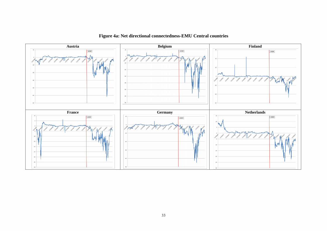
3. Net directional connectedness
The net directional connectedness index provides information about how much each
country’s sovereign bond yield volatility contributes in net terms to other countries’
sovereign bond yield volatilities and, like the full sample dynamic measure presented in
the previous section, also relies on rolling estimation windows. The time varying-
indicators are displayed in Figures 4a and 4b for central and peripheral EMU countries
respectively.
[Insert Figures 4a and 4b here]
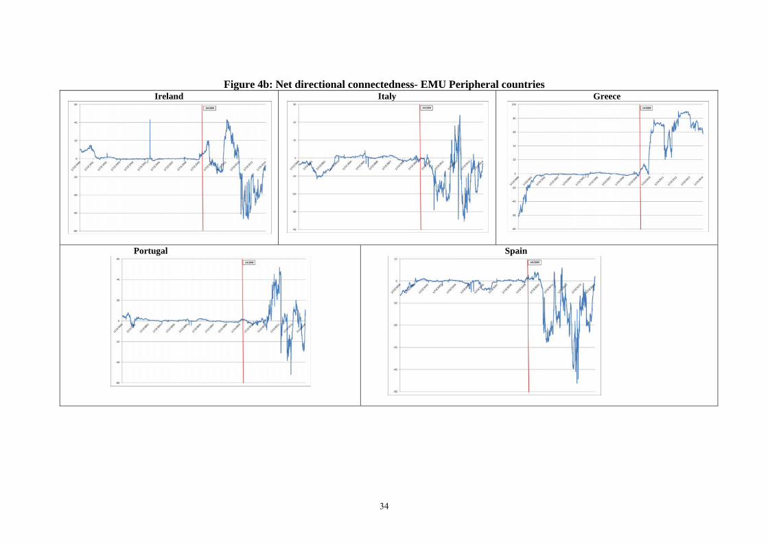
Regarding the whole sample, it is noticeable that in three cases [the Netherlands and
Finland (see Figure 4a) along with Portugal (see Figure 4b)], more than 50% of the
computed values are positive, indicating that during most of the sample period, their
bond yield volatility influenced that of the rest of EMU countries, whereas for the
remaining countries the opposite is true (i.e., they are net receivers during most of the
period). Interestingly, for Germany we obtain negative values in 84% of the sample.
When we split the sample into stability and crisis periods, a different picture emerges.
Before the crisis, with the exception of Portugal, net triggers were mainly central
countries, with a percentage of positive values of 85%, 75%, 65%, 61% and 58% for the
Netherlands, Finland, Belgium, Austria and France, respectively (see Figure 4a).
However, during the crisis period, these countries became net receivers, with negative
values of 100%, 99%, 98%, 95% and 92% for France, Finland, Belgium, Netherlands
and Austria respectively. In this second period, Germany also appears as a net receiver
with a negative value of 100%. Regarding peripheral countries (Figure 4b), four of the
15
five countries studied were net receivers during the stability period, with negative
values of 78%, 57%, 55% and 52% in the cases of Greece, Ireland, Spain and Italy
respectively; during the crisis period Greece and Portugal became net triggers, with
positive values of 99% and 52% respectively.
3.1 Determinants of net directional connectedness
3.1.1 Econometric methodology
After evaluating net directional connectedness, we use panel model techniques to
analyse their determinants. We adopt an eclectic approach and apply a general-to-
specific modelling strategy to empirically evaluate the relevance of the highest number
of variables that have been proposed in the recent theoretical and empirical literature as
potential drivers of EMU sovereign bond yields.
Since the potential determinants are available at monthly or quarterly frequency, we
generate a new dependent variable by computing the monthly average of the daily net
directional connectedness for each country.
3.1.2. Instruments for modelling net directional connectedness
We consider two groups of potential determinants of net directional connectedness:
macroeconomic fundamental variables, and indicators of market sentiments. Regarding
the macro-fundamentals, we use measures of the country’s fiscal position (the
government debt-to-GDP and the government debt-to-GDP, DEB and DEF hereafter),
the overall outstanding volume of sovereign debt (which is considered a good proxy of
liquidity differences among markets, LIQ)10, the current-account-balance-to-GDP ratio
(CAC) as a proxy of the foreign debt and the net position of the country towards the rest
of the world, and the Harmonized Index of Consumer Prices monthly inter-annual rate
of growth (as a measure of inflation, INF and the country’s loss of competitiveness).
With respect to market sentiment proxies, we use the consumer confidence indicator
(CCI) to gauge economic agents’ perceptions of future economic activity, and the
10 Given the large size differences observed between EMU peripheral sovereign debt markets (see Gómez-Puig and Sosvilla-Rivero, 2013), it is likely that the overall outstanding volume of sovereign debt (which is considered a measure of market depth because larger markets may present lower information costs since their securities are likely to trade frequently, and a relative large number of investors may own or may have analyzed their features) might be a good proxy of liquidity differences between markets. Indeed, some of the literature suggests that market size is an important factor in the success of a debt market. Nevertheless, there is another reason to choose this variable: it might capture an additional benefit of large markets to the extent that the ‘‘too big to fail theory’’ (TFTF), taken from the banking system, might also hold in sovereign debt markets.
16
monthly standard deviation of equity returns (EVOL) in each country to capture local
stock market volatility11. A summary with the definition and sources of all the
explanatory variables used is presented in Appendix A.
3.1.3. Empirical results
Our empirical analysis starts with a general unrestricted statistical model including all
explanatory variables to capture the essential characteristics of the underlying dataset.
We use standard testing procedures to reduce its complexity by eliminating statistically
insignificant variables. We check the validity of the reductions at each stage in order to
ensure the congruence of the finally selected model and thus to identify the variables
that best explain the developments.
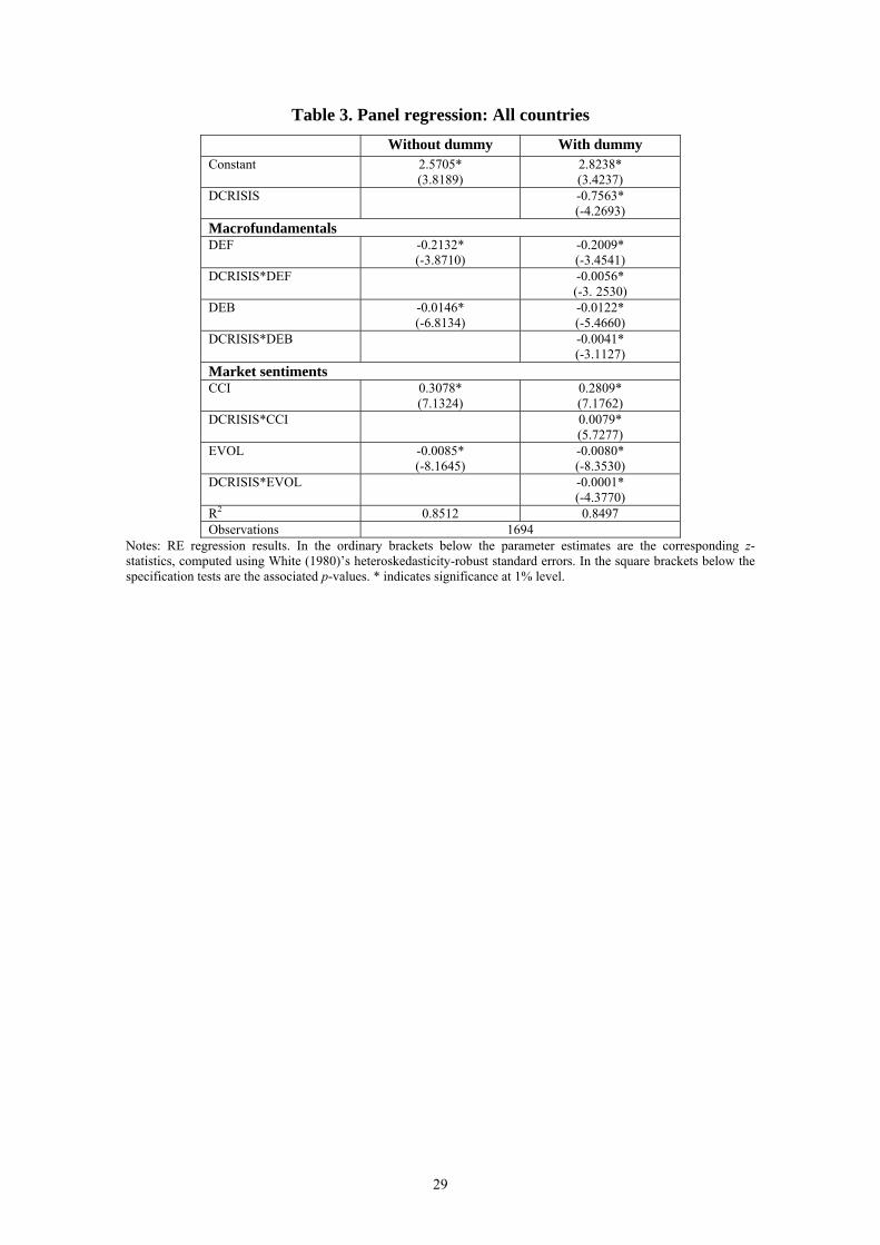
Tables 3 to 5 show the final results for three groups of countries: all 11 EMU countries
under study, EMU central countries, and EMU peripheral countries throughout the
sample period: 2000:01-2014:01. The reason for splitting the sample into these two
groups is that, based on a country-by-country analysis, it can be concluded that EMU
countries under study are not homogeneous but comprise two categories. Therefore, this
division12 makes it possible to differentiate the impact of potential determinants on bond
spreads in core and peripheral countries. We report only the results obtained using the
relevant model in each case13: the Random Effects (RE) model in the case of all EMU
countries and peripheral EMU countries; and the Fixed Effects (FE) model for the
central EMU countries.
[Insert Tables 3 to 5 here]
The first column in these tables do not take into account the dynamic properties of net
directional connectedness; they show the results for the whole period (pre-crisis and
crisis) in order to select the best model for use in the rest of the analysis after having
eliminated statistically insignificant variables. However, since we have previously
detected a potential structural change in April 2009, we analyse the differences in the
significance of the coefficients over time (i.e., during the stability and the crisis
periods).
11 We would expect a positive relationship between the variables CAC, LIQ and CCI with net directional connectedness; whereas the relationship would be negative for the variables DEB, DEF, INF and EVOL. 12 This classification of EMU central and peripheral countries follows the standard division presented in the literature. 13
17
Therefore, in addition to the independent variables chosen a dummy (DCRISIS), which
takes the value 1 in the crisis period (and 0, otherwise) is also introduced in the
estimations, and the coefficients of the interactions between this dummy and the rest of
variables are calculated (see Gómez-Puig, 2006 and 2008). Thus, the marginal effects of
each variable are:
β = β1 + β2DCRISIS
We honestly think that a formal coefficient test H0: β1 = β1 + β2, to assess whether the
impact of independent variables on net directional connectedness changed significantly
with the start of the sovereign debt crisis is unnecessary as long as β2 is significant. So
the marginal coefficients of a variable are:
β = β1 (in the stability period)
β = β1 + β2 (in the crisis period)
The second column in Tables 3 to 5 shows the re-estimation results with the DCRISIS
dummy. Looking across the columns in these tables we see that, when examining the
variables measuring market sentiment in all eleven countries (Table 3) we find a
negative and significant effect for the stock-market volatility (EVOL), whereas, as
expected, the consumer confidence indicator (CCI) presents a positive sign. As for the
local macro-fundamentals, our results suggest a negative impact on the net directional
connectedness of variables measuring the fiscal position (both the debt and the deficit-
to-GDP). Moreover, without exception, all marginal effects register an increase in the
crisis period compared to the pre-crisis one. This rise in the sensitivity to both
fundamentals and market sentiment during the crisis period compared with the pre-crisis
is in line with the previous empirical literature (see Gómez-Puig et al., 2014, among
others).
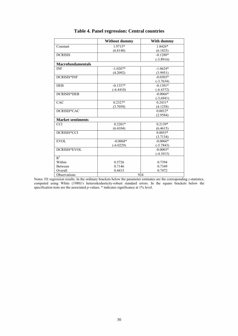
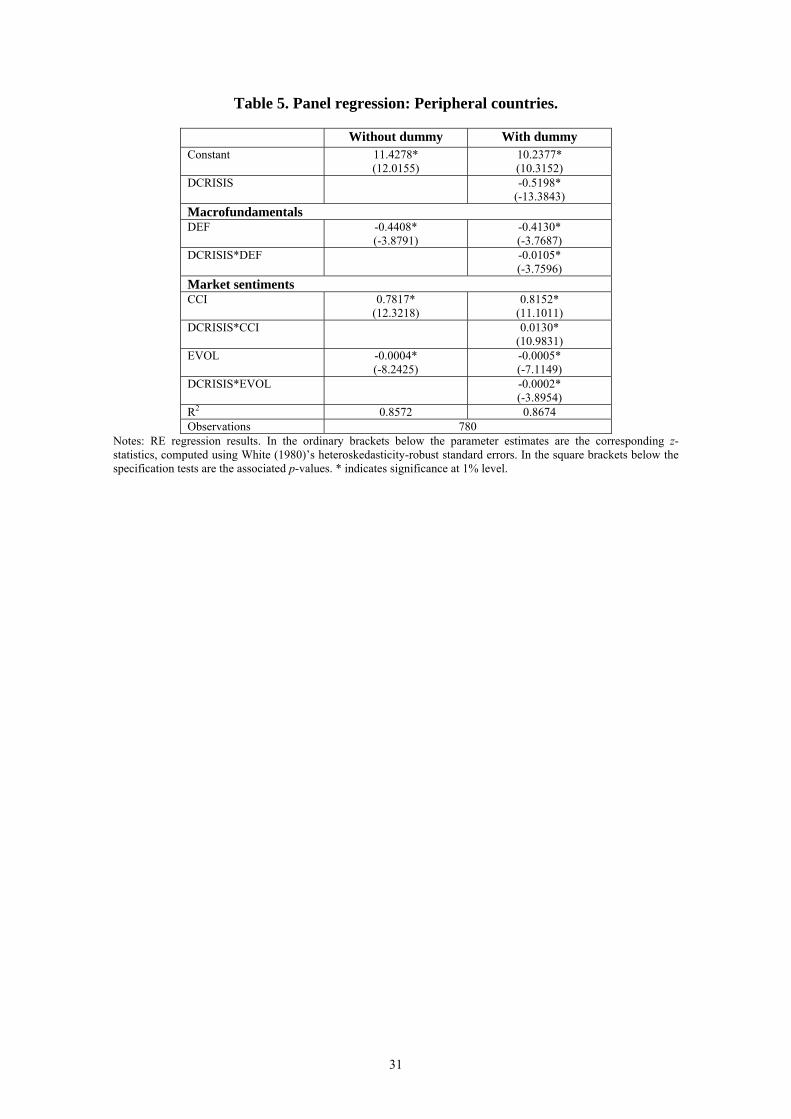
Our analysis also highlights the differences between the two groups of EMU countries,
central and peripheral. In net directional connectedness episodes triggered by peripheral
countries, variables that gauge market participants’ perceptions seem to present a higher
relevance, while macroeconomic fundamentals seem to play a greater role in
18
relationships where central countries are the triggers. In the latter case (see Table 4),
three variables gauging macroeconomic fundamentals are significant with the expected
sign (the loss of competitiveness (INF), the Government deficit-to-GDP (DEB) and the
net position towards the rest of the word (CAC)); whilst in the former (see Table 5) only
the variable that captures the government deficit-to-GDP (DEF) turns out to be
significant. With regard to the variables measuring market sentiment, in the two sub-
samples we find a negative and significant effect for stock-market volatility (EVOL),
whereas, as expected, the consumer confidence indicator (CCI) presents a positive
sign14. Again, without exception, for the two groups of countries all marginal effects
register an increase during the crisis compared to the pre-crisis period.
Therefore, our results indicate that the crisis had a significant impact on the markets’
reactions to financial news, especially in the peripheral countries. In this respect, some
authors have argued that the financial crisis might spread from one country to another
due to market imperfection or the herding behaviour of international investors. A crisis
in one country may give a “wake-up call” to international investors to reassess the risks
in other countries; uninformed or less informed investors may find it difficult to extract
the signal from the falling price and follow the strategies of better informed investors,
thus generating excess co-movements across the markets. The findings presented by
Beirne and Fratscher (2013), for instance, also indicate that for some EMU countries
such as peripheral countries there is strong evidence of this “wake-up call” contagion,
though for other countries there is much less evidence of this kind since the relevance of
macroeconomic fundamentals is higher.
4. Net pair-wise directional connectedness
So far, we have discussed the behaviour of the total connectedness and total net
directional connectedness measures for eleven EMU sovereign debt markets. However,
we have also examined their net pair-wise directional connectedness.
[Insert Figures 5a and 5b here]
14 The only variable that does not turn out to be significant in any of the estimations is our proxy for the market liquidity.
19
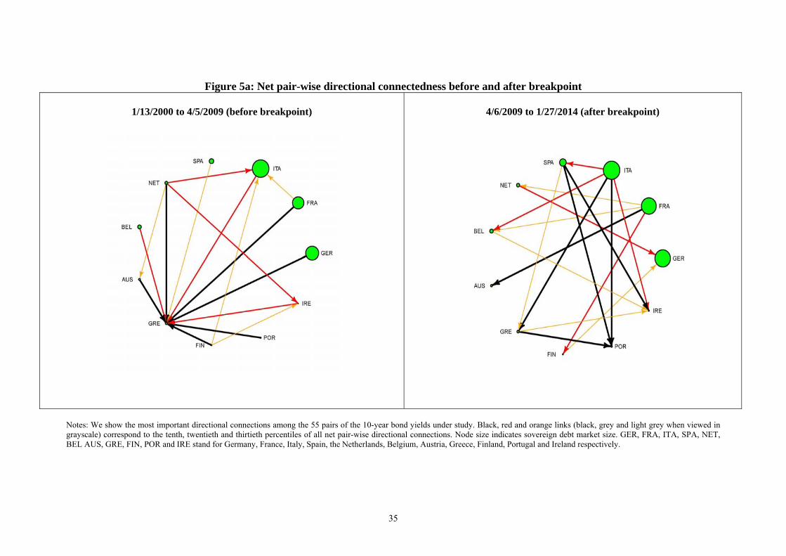
Specifically, Figure 5a displays net pair-wise directional connectedness during the two
detected regimes, whilst Figure 5b presents the results obtained during the five sub-
periods into which the crisis period has been divided.
Both figures present very interesting results. Figure 5a shows that while in the stability
period central countries are the triggers in the connectedness relationships, in the crisis
regime, these relationships are stronger when the trigger is a peripheral country. These
results corroborate those presented in Figure 4 where we plotted net dynamic directional
connectedness in both core and peripheral countries.
In particular, in the stability period, connectedness relationships departing from central
countries accounted for 75% of the total, and in the tenth and twentieth percentile all the
receiver countries are peripheral (Greece, Ireland and Italy). Conversely, in the crisis
period, the connectedness relationships account for 59% of the total when peripheral
countries are the triggers (in the tenth and twentieth percentile, only three relationships
are detected departing from central countries), and although receivers are mostly
peripheral, central countries still account for 41% of the total.
These results are very illuminating since they reinforce the idea that during the first ten
years of currency union, investors’ risk aversion was very low since they overestimated
the healing effect that economically sound central countries might have on the rest of
the Eurozone. However, the situation radically changed with the advent of the crisis;
suddenly, market participants focused their attention on the substantial macroeconomic
imbalances that some peripheral countries presented which not only would eventually
lead them to default, but might also affect central countries that held important shares of
the sovereign assets of those countries (the results suggest that both peripheral and
central countries are net receivers of the connectedness relationships that mainly depart
from peripheral countries).
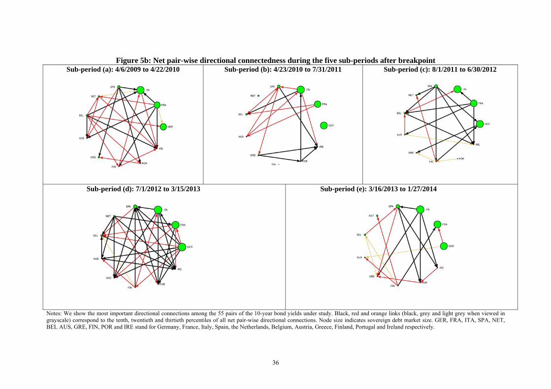
Moreover, the main conclusions that can be drawn from Figure 5b, which displays the
evolution of the net pair-wise directional connectedness during the five crisis sub-
periods, are the following.
During sub-period (a), the period just before the beginning of the euro-area sovereign
debt crisis (marked by Papandreou’s disclosure of Greece’s distressed public finances in
November 2009), we not only detect a significant number (25) of net pair-wise
relationships, but in 72% of the cases central countries are still the triggers. However, an
20
important difference with respect to the pre-crisis period is that peripheral countries
carry less weight as receivers. In this sub-period, they account for 60% of the total,
while the rest (40%) are central countries, showing that the effects of the crisis have
clearly extended to the central countries.
Nonetheless, the situation radically changes in sub-period (b), which includes the bail-
outs of Greece, Ireland and Portugal. In this phase not only does the number of
connectedness relationships decrease from 25 to 14, but their direction changes as well.
In this second sub-period of the crisis, net pair-wise connectedness relationships mainly
occur between peripheral countries, which have a weight of around 71% both as triggers
and as receivers. Besides, it is worth noting that during this phase two central countries
remain disconnected from the rest: the Netherlands and Finland. During sub-period (c),
which includes the support to the Spanish banking sector, Figure 3 shows that the total
level of connectedness still registers a downturn trend; but although the number of
connectedness relationships remains low (15), the amount detected in the tenth
percentile clearly increases (up to 80%). Another significant development is the fact that
central countries recover their role in the relationships as both triggers and receivers
(67% of the total).
However, after Mario Draghi’s statement in July 2012 (sub-period d), a clear shift is
observed. Now, net pair-wise relationships rise to 33 (even more than in sub-period (a))
and not only is the role of central countries as triggers stressed (they represent 76% of
the total), but peripheral countries also recover their role as receivers, returning to the
level of the pre-crisis period (64%). Finally, in the last sub-period (which begins with
the rescue of Cyprus), we again observe a decrease in the number of pair-wise
connectedness relationships; however, the majority of them take place between
peripheral countries, both as triggers (53% of the total) and as receivers (65%).
5. Concluding remarks.
Our analysis, which has focused on the study of connectedness in EMU sovereign bond
yields volatility during the period April 1999 to January 2014, may enhance the
understanding of cross-market volatility dynamics in times of both turbulence and calm,
and may help to assess the risk of crisis transmission. We stress the paper’s important
methodological contribution: that is, the use of the ‘volatility surprise’ component
21
(along with other traditional measures of volatility) to fully apprehend the sensitivity of
financial markets to volatility shocks.
The main contributions of our research can be summarized as follows. In the first step,
we found a system-wide value of 54.23% for the total connectedness between the eleven
countries under study for the full sample period. This level is much lower than that
obtained by Diebold and Yilmaz (2012, 2014) for international financial markets and
US financial institutions respectively. However, it should be understood in the context
of the results obtained in the second step, in which we analyse the dynamic nature of
total net connectedness.
In Figures 1 to 3, which plot total volatility connectedness, we clearly identify two
distinct periods in its evolution which coincide with the evolution of 10-year yields.
Indeed, the existence of these two different regimes in the evolution of connectedness
has been empirically tested and corroborated. In the first period, the level of
connectedness of EMU sovereign debt markets is very high, closely matching the
evolution of 10-year yields. However, in the second period, which begins only a few
months before Papandreou’s government announced Greece’s distressed debt position
(November 2009), connectedness began a downturn trend. Consequently, the substantial
decrease in the level of connectedness in EMU sovereign debt markets, along with the
unfolding of the crisis, may explain its low average value in the static analysis for the
whole sample period.
In the third step, we calculated the net directional connectedness index which provides
information about how much each country’s sovereign bond yield volatility contributes
in net terms to other countries’ sovereign bond yield volatilities. Our empirical evidence
shows that, for the whole sample, in three cases (the Netherlands, Finland and Portugal),
their bond yield volatility influenced that of the rest of EMU countries, whereas the
remaining countries are net receivers. The empirical evidence also suggests that during
the stability period, the triggers of the net connectedness relationships are mainly central
countries, but during the crisis, they are mostly peripheral countries.
In a further step, we used panel data techniques to analyse the drivers of net directional
connectedness in each country. Our results once again highlight the differences between
the two groups of EMU countries, central and peripheral. In net directional
connectedness episodes triggered by peripheral countries, variables that gauge market
22
participants’ perceptions seem to present a higher relevance, while macroeconomic
fundamentals appear to play a greater role in relationships where central countries are
the triggers. Moreover, without exception, all marginal effects register an increase in the
crisis compared to the pre-crisis period.
Finally, in the last step we examined net pair-wise directional connectedness among the
11 EMU countries, both in the two regimes detected and during the five sub-periods in
which the crisis period has been divided. Our findings corroborate the conclusions
drawn from the third step regarding the direction of net connectedness and provide
further insights into both their intensity and their behaviour during the five sub-periods
of the crisis.
Overall, our results support the hypothesis that peripheral countries imported credibility
from central countries during the first ten years of EMU. Nevertheless, the outbreak of
the crisis ushered in a sudden shift in the sentiment of market participants who now paid
more attention to the significant macroeconomic imbalances in some of the peripheral
countries and the possibility of contagion to central countries.
To sum up, the analysis in this paper suggests that the sovereign risk premium increase
in the euro area during the European sovereign debt crisis was not only due to
deteriorated debt sustainability in member countries, but also to a shift in the origin of
connectedness relationships which, as the crisis unfolded, mostly departed from
peripheral countries. In this context, where cross-border financial activity was very
important and market sentiment indicators played a key role in explaining
connectedness relationships triggered by peripheral countries, the risk that the default of
the sovereign/banking sector in one of these countries might spread to other countries
could not be disregarded by financial authorities and policymakers with responsibility
for ensuring financial stability.

23
Appendix A: Definition of the explanatory variables to model net directional connectedness A.1. Variables that measure local macro-fundamentals.
Variable Description Source Net position
vis-à-vis the rest of the
world (CAC)
Current-account-balance-to-GDP Monthly data are linearly interpolated from
quarterly observations.
OECD
Competitiveness (INF)
Inflation rate. HICP monthly inter-annual rate of growth
Eurostat
Fiscal Position
(DEF and DEB)
Government debt-to-GDP and Government deficit-to-GDP. Monthly data are linearly interpolated from quarterly observations.
Eurostat
Market liquidity
(LIQ)
Domestic Debt Securities. Public Sector Amounts Outstanding (billions of US dollars) Monthly data are linearly interpolated from
quarterly observations.
BIS Debt securities statistics.
Table 18
A.2. Variables that measure local market sentiment.
Variable Description Source
Stock Volatility (EVOL)
Monthly standard deviation of the daily returns of each country’s stock market
general index
Datastream
Consumer
Confidence Indicator
(CCI)
This index is built up by the European Commission which conducts regular
harmonised surveys to consumers in each country.
European Commission (DG
ECFIN)
Acknowledgements
The authors thank Maria del Carmen Ramos-Herrera and Manish K. Singh for their
excellent research assistance. This paper is based upon work supported by the
Government of Spain and FEDER under grant numbers ECO2011-23189 and
ECO2013-48326. Simón Sosvilla-Rivero thanks the Universitat de Barcelona and RFA-
IREA for their hospitality. Responsibility for any remaining errors rests with the
authors.
24
References
Acemoglu, D., Ozdaglar, A., Tahbaz-Salehi, A., 2014. Systemic risk and stability in
financial networks. American Economic Review, forthcoming.
Adrian, T., Brunnermeier, M., 2008. CoVaR. Staff Report 348, Federal Reserve Bank of
New York.
Alter, A., Beyer, A., 2014. The dynamics of spillover effects during the European
sovereign debt turmoil. Journal of Banking and Finance 42, 134-153.
Ang, A., Longstaff, F.A. 2013. Systemic sovereign credit risk: Lessons from the US and
Europe. Journal of Monetary Economics 60, 493-510.
Antonakakis, N., Vergos, K., 2013. Sovereign bond yield spillovers in the Euro zone
during the financial and debt crisis. Journal of International Financial Markets,
Institutions and Money 26, 258-272
Apostolakisa, G., Papadopoulos, A. P., 2014. Financial stress spillovers in advanced
economies. Journal of International Financial Markets, Institutions and Money 32, 128-
149
Awartania, B., Maghyerehb, A.I., Al Shiabc, M., 2013. Directional spillovers from the
U.S. and the Saudi market to equities in the Gulf Cooperation Council countries.
Journal of International Financial Markets, Institutions and Money 27, 224-242.
Bai, J., Perron, P. 1998. Estimating and testing linear models with multiple structural
changes. Econometrica 66, 47–78.
Bai, J., Perron, P. 2003. Computation and analysis of multiple structural change models.
Journal of Applied Econometrics 6, 72–78.
Barnes, S., Lane, P. R., Radziwill,. A., 2010. Minimising risks from imbalances in
European banking. Working Paper 828, Economics Department, Organization for
Economomic Cooperation and Development.
Beirne, J., Fratzscher, M., 2013. The pricing of sovereign risk and contagion during the
European sovereign debt crisis. Journal of International Money and Finance 34, 60-82.
Billio, M., Getmansky, M. Lo, A.W., and Pelizzon, L., 2012. Econometric measures of
connectedness and systemic risk in the finance and insurance sectors. Journal of
Financial Economics 104, 535–559.
Chau, F., Deesomsak, R., 2014. Does linkage fuel the fire? The transmission of
financial stress across the markets. International Review of Financial Analysis,
forthcoming.
25
Claeys, P., Vašicek, B. 2014. Measuring bilateral spillover and testing contagion on
sovereign bond markets in Europe. Journal of Banking and Finance 46, 151-165.
Constâncio, V., 2012. Contagion and the European debt crisis. Financial Stability
Review 16, 109-119.
Cronin, D., 2014. The interaction between money and asset markets: A spillover index
approach. Journal of Macroeconomics 39, 185-202
Dasgupta, A., 2004. Financial Contagion Through Capital Connections: A Model of the
Origin and Spread of Bank Panics. Journal of the European Economic Association 2,
1049–84.
Diebold, F. X., Yilmaz, K., 2012. Better to give than to receive: Predictive directional
measurement of volatility spillovers. International Journal of Forecasting 28, 57-66.
Diebold, F. X., Yilmaz, K., 2014. On the network topology of variance decompositions:
Measuring the connectedness of financial firms. Journal of Econometrics 182, 119–134.
Duncan, A. S., Kabundi, A., 2013. Domestic and foreign sources of volatility spillover
to South African asset classes. Economic Modelling 31, 566-573.
Dungey, M., Gajurel, D., 2013. Equity market contagion during the global financial
crisis: Evidence from the World’s eighth largest economies. Working Paper 15, UTAS
School of Economics and Finance.
Engle R., 1993. Technical note: Statistical models for financial volatility. Financial
Analyst Journal 49, 72-78.
Forbes, K., Rigobon, R., 2002. No contagion, only interdependence: Measuring stock
market comovements. Journal of Finance 57, 2223-2261.
Forsberg, L., Ghysels, E., 2007. Why do absolute returns predict volatility so well?
Journal of Financial Econometrics 5, 31-67.
Goldstein, I., Pauzner, A. 2004. Contagion of Self-Fulfilling Financial Crises Due to
Diversification of Investment Portfolios. Journal of Economic Theory 119, 151–83.
Gómez-Puig, M. 2006. Size matters for liquidity: Evidence from EMU sovereign yield
spreads. Economics Letters 90, 156-162.
Gómez-Puig, M. 2008. Monetary integration and the cost of borrowing. Journal of
International Money and Finance 27, 455-479.
Gómez-Puig, M., Sosvilla-Rivero, S., 2013. Granger-causality in peripheral EMU
public debt markets: A dynamic Approach. Journal of Banking and Finance 37, 4627-
4649.
26
Gómez-Puig, M., Sosvilla-Rivero, S., 2014. Causality and contagion in EMU sovereign
debt markets. International Review of Economics and Finance 33, 12-27.
Gómez-Puig, M., Sosvilla-Rivero, S., Ramos-Herrera, M.C. 2014. An update on EMU
sovereign yield spreads drivers in times of crisis: A panel data analysis. The North
American Journal of Economics and Finance 30, 133-153.
Glover, B., and Richards-Shubik, S., 2014. Contagion in the European Sovereign Debt
Crisis. National Bureau of Economic Research Working Paper No. 20567
Gorea, D., Radev, D., 2014. The euro area sovereign debt crisis: Can contagion spread
from the periphery to the core? International Review of Economics and Finance 30, 78-
100.
Kalbaska, A., Gatkowski, M., 2012. Eurozone sovereign contagion: Evidence from the
CDS market (2005–2010). Journal of Economic Behaviour and Organization 83, 657-
673.
Kalemi-Ozcan, S.; Papaioannou, E., Peydró-Alcalde, J. L. 2010. What lies beneath the
Euro’s effect on financial integration? Currency risk, legal harmonization, or trade?
Journal of International Economics 81, 75-88.
Kaminsky, G. L., Reinhart, C. M., 2000. On crises, contagion, and confusion. Journal of
International Economics, 51, 145-168.
Koop, G., Pesaran, M. H., Potter, S. M., 1996. Impulse response analysis in non-linear
multivariate models. Journal of Econometrics 74, 119–147.
Lee, H. C., Chang, S.L., 2013. Finance spillovers of currency carry trade returns, market
risk sentiment, and U.S. market returns. North American Journal of Economics and
Finance 26, 197-216.
Ludwig, A., 2014. A unified approach to investigate pure and wake-up-call contagion:
Evidence from the Eurozone's first financial crisis. Journal of International Money and
Finance 48, 125-146.
Masson, P., 1999. Contagion: Macroeconomic models with multiple equilibria. Journal
of International Money and Finance 18, 587-602.
Metieu, N., 2012. Sovereign risk contagion in the eurozone. Economics Letters 117, 35-
38.
Narayan, P.K. Narayan, S., Prabheesh K.P., 2014. Stock returns, mutual fund flows and
spillover shocks. Pacific-Basin Finance Journal 29, 146-162.
Pesaran, M. H., Shin, Y., 1998. Generalized impulse response analysis in linear
multivariate models. Economics Letters 58, 17–29.
27
Schoenmaker, D., Wagner, W. 2013. Cross-Border Banking in Europe and Financial
Stability, International Finance 16, 1–22
Spiegel, M., 2009a. Monetary and financial integration in the EMU: Push or pull?
Review of International Economics 17, 751-776.
Spiegel, M., 2009b. Monetary and financial integration: Evidence from the EMU.
Journal of the Japanese and International Economies 23, 114-130.
Tsai, I.C., 2014. Spillover of fear: Evidence from the stock markets of five developed
countries. International Review of Financial Analysis 33, 281-288.
Yilmaz, K., 2010. Return and volatility spillovers among the East Asian equity markets.
Journal of Asian Economics 21, 304-313.
Wagner, W. 2010. Diversification at Financial Institutions and Systemic Crises, Journal
of Financial Intermediation 19, 373–86.
Zhou, X., Zhang, W., Zhang, J., 2012. Volatility spillovers between the Chinese and
world equity markets. Pacific-Basin Finance Journal 20, 247-270.
28
Table 1: Schematic connectedness table
x1 x2 ... xN Connectedness from others
x1 Hd11 Hd12
… HNd1 1,
1 1 jd
N
j
Hj
x2 Hd 21 Hd 22
… HNd 2 2,
1 2 jd
N
j
Hj
. . . .
.
.
.
. . .
. .
xN HNd 1
HNd 2
… HNNd Njd
N
j
HNj
,1
Connectedness
to others
N
i
Hid
1 1
1i
N
i
Hid
1 2
2i
…
N
i
HiNd
1
Ni
N
ji
HiNd
N 1,
1
Ni
Table 2: Full-sample connectedness
GER
FRA
ITA
SPA
NET
BEL
AUS
GRE
FIN
POR
IRE
Contribution From Others
GER 20.05 18.39 2.83 1.34 17.09 9.79 13.04 0.08 17.20 0.07 0.12 79.95
FRA 10.38 29.44 1.10 0.29 14.93 13.11 15.48 0.41 14.71 0.09 0.07 70.56
ITA 0.52 0.36 68.00 25.27 0.67 3.08 0.30 0.00 0.76 0.13 0.90 32.00
SPA 0.22 0.03 34.03 61.69 0.20 1.69 0.08 0.08 0.34 0.38 1.26 38.31
NET 12.24 18.85 2.74 0.50 20.64 12.72 14.75 0.01 17.38 0.16 0.02 79.36
BEL 4.89 10.26 12.36 4.91 8.97 41.10 8.48 0.34 8.41 0.10 0.16 58.90
AUS 9.13 20.03 1.06 0.19 15.11 14.00 23.83 0.55 15.93 0.16 0.01 76.17
GRE 0.10 0.23 2.89 2.13 0.10 0.12 0.01 92.66 0.03 1.05 0.67 7.34
FIN 12.09 18.65 3.23 1.04 17.09 11.55 15.74 0.10 20.39 0.09 0.03 79.61
POR 0.01 0.37 10.13 13.34 0.04 0.04 0.36 10.44 0.04 54.45 10.80 45.55
IRE 0.07 0.36 8.28 10.23 0.00 1.02 0.12 2.70 0.01 6.04 71.18 28.82
Contribution To Others
71.23 74.83 53.63 48.99 78.24 62.02 74.15 13.69 78.58 13.17 16.48 54.23
Net Contribution (To –From)
Others
-8.72
4.27
21.63
10.68
-1.12
3.13
-2.02
6.34
-1.03
-2.37
-2.34
Note: GER, FRA, ITA, SPA, NET, BEL AUS, GRE, FIN, POR and IRE stand for Germany, France, Italy, Spain, the Netherlands, Belgium, Austria, Greece, Finland, Portugal and Ireland respectively.
29
Table 3. Panel regression: All countries
Without dummy With dummy Constant 2.5705*
(3.8189) 2.8238* (3.4237)
DCRISIS -0.7563* (-4.2693)
Macrofundamentals DEF -0.2132*
(-3.8710) -0.2009* (-3.4541)
DCRISIS*DEF -0.0056* (-3. 2530)
DEB -0.0146* (-6.8134)
-0.0122* (-5.4660)
DCRISIS*DEB -0.0041* (-3.1127)
Market sentiments CCI 0.3078*
(7.1324) 0.2809* (7.1762)
DCRISIS*CCI 0.0079* (5.7277)
EVOL -0.0085* (-8.1645)
-0.0080* (-8.3530)
DCRISIS*EVOL -0.0001* (-4.3770)
R2 0.8512 0.8497 Observations 1694
Notes: RE regression results. In the ordinary brackets below the parameter estimates are the corresponding z-statistics, computed using White (1980)’s heteroskedasticity-robust standard errors. In the square brackets below the specification tests are the associated p-values. * indicates significance at 1% level.
30
Table 4. Panel regression: Central countries
Without dummy With dummy Constant 1.9715*
(6.8140) 1.8426* (6.1825)
DCRISIS -0.1288* (-3.8916)
Macrofundamentals INF -1.0207*
(4.2092) -1.0624* (3.9951)
DCRISIS*INF -0.0303* (-3.7634)
DEB -0.1357* (-6.4410)
-0.1301* (-6.4372)
DCRISIS*DEB -0.0066* (-3.6941)
CAC 0.2327* (3.7058)
0.2431* (4.1258)
DCRISIS*CAC 0.0012* (2.9584)
Market sentiments CCI 0.2201*
(6.4104) 0.2139* (6.4615)
DCRISIS*CCI 0.0053* (3.7134)
EVOL -0.0068* (-6.0229)
-0.0066* (-5.7843)
DCRISIS*EVOL -0.0003* (-4.1013)
R2
Within Between Overall
0.5726 0.7146 0.4415
0.7394 0.7349 0.7472
Observations 924 Notes: FE regression results. In the ordinary brackets below the parameter estimates are the corresponding z-statistics, computed using White (1980)’s heteroskedasticity-robust standard errors. In the square brackets below the specification tests are the associated p-values. * indicates significance at 1% level.
31
Table 5. Panel regression: Peripheral countries.
Without dummy With dummy Constant 11.4278*
(12.0155) 10.2377* (10.3152)
DCRISIS -0.5198* (-13.3843)
Macrofundamentals DEF -0.4408*
(-3.8791) -0.4130* (-3.7687)
DCRISIS*DEF -0.0105* (-3.7596)
Market sentiments CCI 0.7817*
(12.3218) 0.8152*
(11.1011) DCRISIS*CCI 0.0130*
(10.9831) EVOL -0.0004*
(-8.2425) -0.0005* (-7.1149)
DCRISIS*EVOL -0.0002* (-3.8954)
R2 0.8572 0.8674 Observations 780
Notes: RE regression results. In the ordinary brackets below the parameter estimates are the corresponding z-statistics, computed using White (1980)’s heteroskedasticity-robust standard errors. In the square brackets below the specification tests are the associated p-values. * indicates significance at 1% level.
32
Figure 1: Daily 10-year sovereign yields in EMU countries and rolling total connectedness:
Figure 2: Rolling total connectedness throughout the period (1/13/2000-1/27/2014)
Figure 3: Rolling total connectedness after the breakpoint (6/4/2009-1/27/2014)
33
Figure 4a: Net directional connectedness-EMU Central countries
Austria
Belgium Finland
France Germany Netherlands
34
Figure 4b: Net directional connectedness- EMU Peripheral countries Ireland
Italy
Greece
Portugal
Spain
35
Figure 5a: Net pair-wise directional connectedness before and after breakpoint
1/13/2000 to 4/5/2009 (before breakpoint)
4/6/2009 to 1/27/2014 (after breakpoint)
Notes: We show the most important directional connections among the 55 pairs of the 10-year bond yields under study. Black, red and orange links (black, grey and light grey when viewed in grayscale) correspond to the tenth, twentieth and thirtieth percentiles of all net pair-wise directional connections. Node size indicates sovereign debt market size. GER, FRA, ITA, SPA, NET, BEL AUS, GRE, FIN, POR and IRE stand for Germany, France, Italy, Spain, the Netherlands, Belgium, Austria, Greece, Finland, Portugal and Ireland respectively.
36
Figure 5b: Net pair-wise directional connectedness during the five sub-periods after breakpoint Sub-period (a): 4/6/2009 to 4/22/2010
Sub-period (b): 4/23/2010 to 7/31/2011
Sub-period (c): 8/1/2011 to 6/30/2012
Sub-period (d): 7/1/2012 to 3/15/2013
Sub-period (e): 3/16/2013 to 1/27/2014
Notes: We show the most important directional connections among the 55 pairs of the 10-year bond yields under study. Black, red and orange links (black, grey and light grey when viewed in grayscale) correspond to the tenth, twentieth and thirtieth percentiles of all net pair-wise directional connections. Node size indicates sovereign debt market size. GER, FRA, ITA, SPA, NET, BEL AUS, GRE, FIN, POR and IRE stand for Germany, France, Italy, Spain, the Netherlands, Belgium, Austria, Greece, Finland, Portugal and Ireland respectively.