IN DEGREE PROJECT MATHEMATICS,SECOND CYCLE, 30 CREDITS

, STOCKHOLM SWEDEN 2018

Financial Risk Profiling using Logistic Regression

LOVISA EMFEVID

HAMPUS NYQUIST

KTH ROYAL INSTITUTE OF TECHNOLOGYSCHOOL OF ENGINEERING SCIENCES

Financial Risk Profiling using Logistic Regression LOVISA EMFEVID HAMPUS NYQUIST

Degree Projects in Financial Mathematics (30 ECTS credits) KTH Royal Institute of Technology year 2018 Supervisors at Investmate AB: Andreas Lindell Supervisor at KTH: Boualem Djehiche Examiner at KTH: Boualem Djehiche

TRITA-SCI-GRU 2018:253 MAT-E 2018:53

Royal Institute of Technology School of Engineering Sciences KTH SCI SE-100 44 Stockholm, Sweden URL: www.kth.se/sci

!

Financial Risk Profiling using Logistic Regression

Abstract As automation in the financial service industry continues to advance, online investment advice has emerged as an exciting new field. Vital to the accuracy of such service is the determination of the individual investors’ ability to bear financial risk. To do so, the statistical method of logistic regression is used. The aim of this thesis is to identify factors which are significant in determining a financial risk profile of a retail investor. In other words, the study seeks to map out the relationship between several socioeconomic- and psychometric variables to develop a predictive model able to determine the risk profile. The analysis is based on survey data from respondents living in Sweden. The main findings are that variables such as income, consumption rate, experience of a financial bear market, and various psychometric variables are significant in determining a financial risk profile. Keywords: logistic regression, principal component analysis, stepwise selection, cross validation, risk tolerance, risk capacity, risk aversion, financial risk profile

!

Finansiell riskprofilering med logistisk regression Sammanfattning I samband med en ökad automatiseringstrend har digital investeringsrådgivning dykt upp som ett nytt fenomen. Av central betydelse är tjänstens förmåga att bedöma en investerares förmåga till att bära finansiell risk. Logistik regression tillämpas för att bedöma en icke-professionell investerares vilja att bära finansiell risk. Målet med uppsatsen är således att identifiera ett antal faktorer med signifikant förmåga till att bedöma en icke-professionell investerares riskprofil. Med andra ord, så syftar denna uppsats till att studera förmågan hos ett antal socioekonomiska- och psykometriska variabler. För att därigenom utveckla en prediktiv modell som kan skatta en individs finansiella riskprofil. Analysen genomförs med hjälp av en enkätstudie hos respondenter bosatta i Sverige. Den huvudsakliga slutsatsen är att en individs inkomst, konsumtionstakt, tidigare erfarenheter av abnorma marknadsförhållanden, och diverse psykometriska komponenter besitter en betydande förmåga till att avgöra en individs finansiella risktolerans.

! 3!

!

Table of Contents 1"Introduction"...................................................................................................................."1!

2"Theoretical"frame"of"reference"........................................................................................"2!2.1! Ordinal"variables"............................................................................................................."2!

2.1.1! Transformation!..................................................................................................................!2!2.2! Spearman’s"correlation"..................................................................................................."3!2.3! Logistic"regression"model"................................................................................................"4!

Definition!2.3.1! Binomial!distribution!.........................................................................................!4!Definition!2.3.2! Logit!link!function!..............................................................................................!4!

2.4! Wald"test"........................................................................................................................"5!2.5! LikelihoodCratio"chiCsquare"test"......................................................................................."6!2.6! Univariate"ANOVA".........................................................................................................."6!

2.6.1! Two!sample!t?test!..............................................................................................................!6!2.8! Variable"selection"..........................................................................................................."7!

2.8.1! AIC!.....................................................................................................................................!7!2.8.2! Confusion!matrix!&!ROC!....................................................................................................!8!2.8.3! Subset!selection!.................................................................................................................!9!

2.9! Resampling"methods"......................................................................................................."9!2.9.1! Leave?one?out!cross?validation!.........................................................................................!9!2.9.2! K?fold!cross?validation!.....................................................................................................!10!

2.10! Literature"study"............................................................................................................"10!2.10.1! Financial!risk!tolerance:!a!psychometric!review!.........................................................!10!2.10.2! Investor!risk!profiling:!an!overview!.............................................................................!11!2.10.3! Portfolio!Selection!using!Multi?Objective!Optimisation!..............................................!12!

2.11! Regulatory"environment"..............................................................................................."13!3"Method".................................................................................................................................."14!3.1! Dependent"variable"......................................................................................................"14!

Definition!3.1.1! Psychometric!test!score!(t?score)!....................................................................!14!Definition!3.1.2! Dependent!variable!II!......................................................................................!15!

3.2! Explanans"....................................................................................................................."15!3.3! Indicator"variables"........................................................................................................"15!

Definition!3.3.1! Gender!.............................................................................................................!15!Definition!3.3.2! Children!...........................................................................................................!16!Definition!3.3.3! Sole!custody!....................................................................................................!16!Definition!3.3.4! Higher!education!.............................................................................................!16!Definition!3.3.5! Bear!market!experience!..................................................................................!16!Definition!3.3.6! Overconfidence!...............................................................................................!16!Definition!3.3.7! Leverage!..........................................................................................................!16!

3.4! Categorical"variables"....................................................................................................."17!Definition!3.4.1! Age!group!........................................................................................................!17!Definition!3.4.2! Occupation!......................................................................................................!17!Definition!3.4.3! Buy!scheme!.....................................................................................................!17!Definition!3.4.4! Risk!preference!&!profile!.................................................................................!17!Definition!3.4.5! Financial!stamina!.............................................................................................!18!Definition!3.4.6! Financial!literacy!level!.....................................................................................!18!

"

! 4!

!

3.5! Quantitative"variables"..................................................................................................."18!Definition!3.6.1! Normalized!income!.........................................................................................!18!Definition!3.6.2! Normalized!cost!...............................................................................................!18!Definition!3.6.3! Burn!ratio!........................................................................................................!18!Definition!3.6.4! Normalized!wealth!..........................................................................................!19!Definition!3.6.5! Loan!to!value!(LTV)!ratio!.................................................................................!19!Definition!3.6.6! Asset!class!........................................................................................................!19!Definition!3.6.7! Debt!ratio!........................................................................................................!19!

3.7! Psychometric"variables"................................................................................................."19!

4"Data".............................................................................................................................."20!4.1! Quantitative"data"sample".............................................................................................."20!

4.1.1! QQ?plots!and!scatter!plots!...............................................................................................!20!4.1.2! Sample!statistics!..............................................................................................................!22!4.1.3! Collinearity!.......................................................................................................................!23!4.1.4! Grouping!the!variables!....................................................................................................!25!4.1.6! Boxplots!...........................................................................................................................!27!

4.2! Qualitative"variables"....................................................................................................."28!4.2.1! Two!sample!t?test!............................................................................................................!29!4.2.2! F?test!................................................................................................................................!29!4.2.3! Boxplots!...........................................................................................................................!30!

4.3! Psychometric"variables"................................................................................................."31!5"Calibrating"the"model"............................................................................................................."36!5.1! Variable"selection"(method"I)"........................................................................................"36!

5.1.1! Subset!selection!–!quantitative!variables!........................................................................!37!5.1.2! Subset!selection!–!qualitative!variables!...........................................................................!38!5.1.3! Subset!selection!–!ordinal!variables!................................................................................!40!5.1.4! Final!subset!selection!......................................................................................................!41!

5.2! Variable"selection"(method"II)"......................................................................................."43!Principal"Component"Analysis"(PCA)".........................................................................................."44!5.3"! Comparing"the"models".................................................................................................."48!

6"Analysis"and"conclusion"................................................................................................."50!

7"Discussion"and"recommendation"..................................................................................."52!

8"References"....................................................................................................................."53!8.1! Literature"......................................................................................................................"53!8.2! Websites"......................................................................................................................."54!

9."Appendix"......................................................................................................................"54!A1"–"Demographics"..................................................................................................................."54!A2"–"Prior"experience"&"attitude"to"risk"....................................................................................."55!A3"–"Financial"literacy"................................................................................................................"56!A4"–"Psychometric"part"............................................................................................................."58!

! 1!

!

1 Introduction In recent years, the concept of a ‘robot-advisor’ has become a more visible phenomenon, and is today considered a new investment vehicle, readily available for the general public. A fintech company is therefore interested in investigating whether methods from statistical learning, multivariate statistics, and behavioural finance can be applied to develop a statistical model, used to assign a financial risk profile to a retail investor. The idea behind a business to customer robot-advisory is that a retail investor through a survey method is assigned a risk profile. In other words, a survey is used to extract some information from the investor, whereby an appropriate investment portfolio is recommended. However, some experimental studies have shown that there seems to be a discrepancy between an investor’s actual asset allocation, and the assigned risk profile, Klement (2015). Furthermore, today’s regulatory environment seems to look favourably upon this new phenomenon, however, some minimum requirements are to be met. The purpose of this thesis is thus to first conduct a literature study, in order to map out a battery of survey questions, collect data, and to investigate the explanatory power of the items used in the survey. Following this, a logistic regression model is used to classify the risk level of a retail investor, and two methods for variable selection is presented, ending with three candidate models that could be used. To fulfil this goal, the layout of the thesis can be seen as follows. First a theory section will outline the theoretical frame of reference, stating the underlying frameworks used in this thesis. Secondly, a methodology section follows, where proper definitions of the variables used in the model are presented. Thirdly, a data section summarizes the data sample and its statistics. Ensuing this, a section dedicated to variable selection comes. Lastly, analysis and conclusion takes place, summarizing the main findings, and finally a discussion of potential future research takes place.

! 2!

!

2 Theoretical frame of reference In this section the theoretical frame of reference used to develop the model, will be presented. As the client requested a logistic regression model to be used when classifying the level of risk tolerance, the underlying assumptions of this model will be presented in this section. Furthermore, as the sample data consist of few observations and many variables, a factor analysis is applied in an attempt to reduce the number of variables to make the analysis simpler. Thus, a presentation of principal component will follow. As the accuracy of a binary classifier is commonly evaluated by the use of a confusion matrix and illustrated by a ROC curve, this will also be presented. As this model is intended to be used in the business to consumer market, some regulatory standards are expected to be met. To achieve this goal, a brief literature study was first conducted, (Section 2.10). Additionally, the key points from today’s regulatory environment will also be presented in (Section 2.11). 2.1 Ordinal variables We say that a random variable is an ordinal variable if it is a discrete variable for which the possible outcomes are ordered. For example:

! ∈ high&school, B. Sc. , M. Sc.

0 ∈ low&income, average&income, high&income 2.1.1 Transformation If an ordinal variable has an even number of outcomes, then we say that the variable is de-centralized, and vice versa if it has an odd number of outcomes. Let ! be an ordinal random variable taking the following four outcomes 1, 2, 3, 4 , one can then define a new ordinal random variable 0:

0 =&&0&>?&! ∈ 1, 2&&&1&>?&! ∈ 3, 4

Moreover, by using a similar approach, a centralized ordinal variable can be transformed into one with three distinct outcomes. For example: if X is some ordinal random variable, e.g. X ∈ 1, 2, 3, 4, 5 , then if

! ∈ 1, 2 , let&0 = 1

! ∈ 3 , let&0 = 2

! ∈ 4, 5 , let&0 = 3 Put differently, an ordinal variable with five outcomes, can be transformed into one with three outcomes.

! 3!

!

2.2 Spearman’s correlation Before calculating Spearman’s rank order correlation coefficient, one should be aware of two inherent assumptions: i) the variables are measured on an ordinal-, interval- or a ratio scale; ii) the two variables have a monotonic relationship, i.e. the variables increase (or decrease) in the same direction, but not necessarily at a constant rate. Let ! and 0 be two ordinal variables, whose outcomes are denoted by CD, CE &…&CG and HD, HE &…&HG respectively, then the Spearman correlation coefficient IJ is defined as follows

IJ =KLM INO, INPQRSTQRSU

where INO and INP refers to the rank of ! and 0. Let the difference in rank of observation > be denoted in the following way

VW = IN !W − IN 0W The Spearman rank correlation is then defined as follows

IJ = 1 −6 VWG

WZD

[ [E − 1

In the case of a tied rank, i.e. if the following occurs:

CW = C\, > ≠ ^

or

HW = H\, > ≠ ^

! 4!

!

2.3 Logistic regression model In the binomial logistic regression model, the dependent variable 0 has two distinct outcomes:

0 ∈ 0, 1 Usually, the outcome can be seen as either a failure or a success, 0, 1 . The independent variables, !D, !E, …!_, are also some binary variables. I.e.

!\ ∈ 0,1 , ^ = 1,2…` In other words, if we sample [ number of outcomes from one of the independent variables, then we realize that the probability of drawing a number of successes, can be modelled by using the probability density function (p.d.f.) of a binomial distribution. Definition 2.3.1 Binomial distribution

If a random variable ! follows a binomial distribution with the parameters [ ∈ Ν and c ∈ 0,1 . Then its p.d.f. is given by the following expression

P ! = a =[ace 1 − c Gfe,

where [ are the number of outcomes, and a the number of successes. Denoted !~B [, c . Definition 2.3.2 Logit link function

Let c denote some “posterior” probability, i.e.

c = h 0 = 1 i = j &&&&&&&&&& The “log odds ratio”, a.k.a. the logit link function, can then be defined in the following way.

logit c = logc

1 − c

To model this odds ratio, the logistic regression model equates the logit transform, i.e. the log-odds of the probability of a success (logit link function), to a linear function in the following way:

logit c = g k &&&&&&&&&&(2.3.2) where

g k = no + ne!e

_

eZD

! 5!

!

The unknown parameters βr in the logistic regression is estimated using the maximum likelihood estimation. Having a sample size of s trials, the parametrization of the probability density function can be expressed as follows.

? t u =[W!

HW! [W − HW

w

WZD

xWyz 1 − xW Gzfyz&&&&&&&&&&(2.3.3)

> = 1,2…s

HW = CW,Gz

WZD

&&&&&&&&&&HW ⊂ 0,M

Where HW corresponds to the number of successes in trial >. Moreover, let [W denote the number of possible outcomes in trial >, and xW the “true probability” of a success in trial >, respectively. In other words, we want to maximize some likelihood ratio. To do this, first note that the factorial terms in (2.3.3) can be treated as a some constant. Doing so, the likelihood ratio can be expressed as

| t u = xWyz 1 − xW Gzfyz

w

WZD

A further presentation of the numerical procedure used to estimate the parameters is not assumed to be needed. 2.4 Wald test To test the statistical significance of a specific parameter in the model, a Wald test can be conducted. The Wald test statistic is defined as follows:

}\ =n\

~�(n\)&&&&&&&&&&

Where n\ is the maximum likelihood estimation of the coefficient for the ^:th independent parameter, and ~�(n\) is the standard error of the estimated coefficient. When the sample size is large then }\ is approximately standard normal distributed, and the following hypothesis can be tested:

Äo:&n\ = 0&

vs the alternative

ÄD: n\ &&≠ 0&

! 6!

!

The null hypothesis is rejected at an Ç-significance level if }\ > ÑÖ/E, where ÑÖ/E is the Ç-quantile of the standard normal distribution. 2.5 Likelihood-ratio chi-square test In a logistic regression setting, one is usually interested in comparing whether adding a new independent variable to the model makes any significance difference. To do so, a likelihood-ratio chi-square test can be used. More specifically, a likelihood ratio is calculated in the following way

|RáàWâ = −2|GäJàäã|åçéé

&&&&&&&&&

where |åçéé denotes the likelihood when fitting the full model, and |GäJàäã denotes the likelihood when fitting a nested model, i.e. a model that contains the same variables as in the full model, except that one or more of the variables from the full model have been removed. In accordance to Hosmer (2013), this ratio can in turn be seen as a chi-squared distributed random variable. Where the degrees of freedom (df) of a model is equal to the number of coefficients in the model. Therefore, the degrees of freedom of the ratio, is the difference in the number of coefficients in the full and nested model, i.e. V?åçéé − V?GäJàäã. In other words, the following hypothesis can then be tested

Ho: the&nested&model&is&the&"best" model

versus

HD: the&full&model&is&the&"best" model 2.6 Univariate ANOVA ANOVA is the abbreviation for “Analysis of Variance”. In this particular setting the purpose is to investigate whether two random variables can be considered as two distinct ones, or whether they possess the same discriminatory power with respect to some underlying measurement. For example, imagine some experimental design, e.g. dividing identical experimental units into two categories, one receiving treatment A and the other receiving treatment B. Of interest would then be to investigate whether a “treatment effect” seems to be persistent. 2.6.1 Two sample t-test The following technique can be used to investigate whether two subpopulation has a significant and different mean value. Let C\ denote an outcome from subpopulation one, ^ = 1,2…[D, with [D different outcomes, and H\ an outcome from subpopulation two, ^ = 1,2…[E.

! 7!

!

If the assumption of equal standard deviation for the two populations seems to be violated, i.e. if îD ≈ îE seems unlikely, one can instead calculate the ‘pooled standard deviation’ for the two populations, îñ as follows,

îñE =[D − 1 îDE + [E − 1 îEE

[D + [E − 2

With equal variances, one can use the t-statistic below to test the hypothesis

Äo:&!D = !E

versus

ÄD:&!D ≠ !E

ó =CD − CE

îDE[D+ îEE[E

&&&&&&&&&&(2.6.1)

by comparing ó with óGfD Ç/2 , the upper 100 Ç/2 th percentile of a t-distribution with [D − 1 + [E − 1 degrees of freedom.

When the assumption of equal variances seems unlikely, one just replaces îDE and îEE in (2.6.1) with îñE and calculates the degrees of freedom, M, in the following way

M =îDE/[D + îEE/[E E

îDE/[D E

[D − 1+ îEE/[E E

[E − 1

2.8 Variable selection In this section, some common metrics that can be used to evaluate the quality of the fitted model will be presented. 2.8.1 AIC The Aikake’s information criteria is a measure of the goodness of fit for a model. The metric includes the log likelihood function of the estimated model, and adds a penalty term for adding extra parameters. Thus, one can calculate the AIC for models containing different parameters, and thereby vis-à-vis compare the attractiveness of each. The model with the lowest value is the one that best fits the data, and is preferred over the other. Below follows a definition.

òôö = 2a − 2õ[ |

! 8!

!

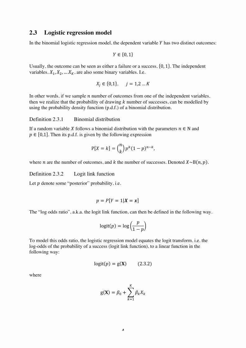
Where a represents the number of parameters in the model and | is the estimated likelihood function of the fitted model. 2.8.2 Confusion matrix & ROC A confusion matrix is a common way to evaluate classification models by measuring actual and predicted values in tabular format: it displays the number of correctly predicted variables and the number of incorrectly predicted values for each category, see Figure 2.1, below.

Figure 2.1: confusion matrix indicating correctly and wrongfully predicted outcomes

Using the true positive value (TP), false positive values (FP), true negative value (TN) and false negative (FN), the following metrics can be calculated, Grable (2017):

•! Sensitivity = TP / (TP+TN) - Refers to how well a test correctly identifies the presence of an attribute.

•! Specificity = TN / (FN+TN) - The proportion of test takers without the attribute

•! Item accuracy = (TP + TN) / (TP+TN+FP+FN) - The proportion of cases that are true to the total number of cases

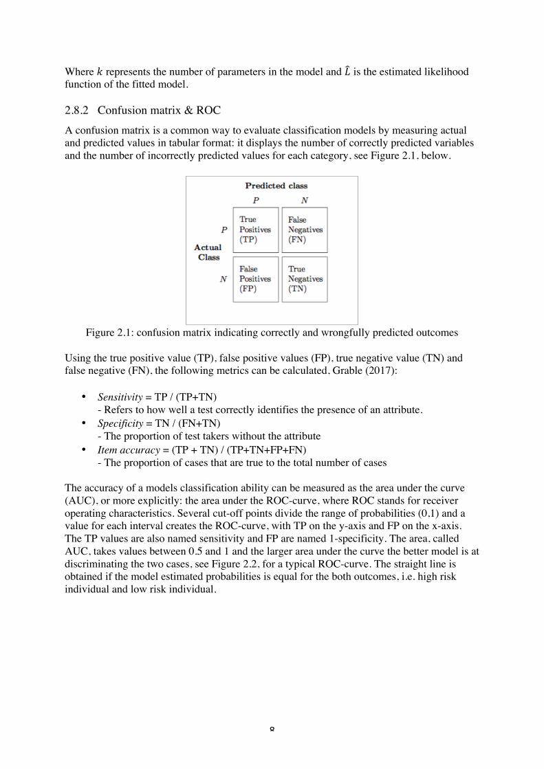
The accuracy of a models classification ability can be measured as the area under the curve (AUC), or more explicitly: the area under the ROC-curve, where ROC stands for receiver operating characteristics. Several cut-off points divide the range of probabilities (0,1) and a value for each interval creates the ROC-curve, with TP on the y-axis and FP on the x-axis. The TP values are also named sensitivity and FP are named 1-specificity. The area, called AUC, takes values between 0.5 and 1 and the larger area under the curve the better model is at discriminating the two cases, see Figure 2.2, for a typical ROC-curve. The straight line is obtained if the model estimated probabilities is equal for the both outcomes, i.e. high risk individual and low risk individual.

! 9!

!

Figure 2.2: example of a receiver operating characteristic curve

The area under the curve is calculate with the trapezoidal rule, and is helpful for comparing different models, there is no direct rule of what constitutes a good AUC value, but the following values are presented and can be considered as a rule of thumb when evaluating the AUC values, Hosmer, et al (2013).

•! úùö& = &0.5, this suggests no discrimination - so we might as well flip a coin •! 0.5& < &úùö& < &0.7, suggests poor discrimination - not much better than a coin flip •! 0.7& ≤ &úùö& < &0.8, we consider this as acceptable discrimination •! úùö ≥ 0.9, we consider this as outstanding discrimination

2.8.3 Subset selection Meta text: present the algorithm of forward- and backward subset selection. 2.9 Resampling methods The purpose of this section is to present two common re-sampling methods used to approximate the test error. That is, when the sample size is too small, and all data needs to be used to train the model, a common approach is to use a resampling method to approximate the test error. As our sample size is relatively small, a re-sampling method will be used, and a brief presentation will therefor follow. 2.9.1 Leave-one-out cross-validation The aim of this method is to approximate the test error. To do so, the sample is divided into two subsets, one containing a single observation CD, HD that is used for the validation set, and the remaining CE, HE , … , CG, HG making up the training set. In other words, the model is fit on the [ − 1 training observations, and a prediction HD is made for the excluded observation. The process is then repeated by selecting CE, HE for the validation set, and including CD, HD to the training set. Thus, after performing [ number of iteration, we have [ approximations of what could have constituted a test error, making it possible to make an estimate of the “true” test error. In a classification setting, one way to measure the test error, is to count the number of miss-classifications. If we let �úúW denote a dummy variable, taking the value of one if a test

! 10!

!

prediction resulted in a misclassification, and zeros otherwise, one could estimate the accuracy ratio in the following way:

ö§(G) =1[

�úúW

G

WZD

2.9.2 K-fold cross-validation When one has a larger sample size, the number of iterations needed to approximate the test error by using the leave-one-out technique presented in the previous section, can be quite time consuming. To account for this, one can instead use the method of k-fold cross validation. This approach involves randomly dividing the data set into k different subsets, of roughly equal size. The model is then trained on k-1 of the sets, whereas the remaining set is used to compute the test error. This process is then repeated a times, each time treating one different set as the validation set. The k-fold test error is then estimated by taking the average of all validation sets. 2.10 Literature study In this section a literature study related to the subject of financial risk profiling will be presented. The main purpose is to re-iterate some interesting findings that can be used when going further and constructing the survey, but also to give the reader some initial taste of the subject. 2.10.1 Financial risk tolerance: a psychometric review In this sub-section a brief outline of what was said in the article written by Grable, E., J. (2017) will be stated. The main purpose of the article is to give professionals within the investment advisory community some guidance, regarding the main principles to consider when administering a financial risk-profiling survey. To start off, there are two main paradigms that people tend to subscribe to when conducting a survey: classical test theory and item response theory, abbreviated CCT and IRT. In this case, the author focused on the former. Moreover, there are two psychometric concepts used to evaluate the quality of a test: validity and reliability. Validity refers to the extent to which a measurement tool measures the attribute it was intended to evaluate, and reliability refers to the measurement error associated with a test. To elaborate, one can imagine that a test score can be divided into two parts:

ù•î¶IM¶V&îKLI¶ = ßI®¶&îKLI¶ + ©¶™î®I¶´¶[ó&¶IILI Where the measurement error depends on environmental factors, e.g. the mood or health situation of the exam taker. However, the primary source of measurement error comes from poorly designed tests with ambiguous wording. As a general rule, a valid test usually assures reliability, while the opposite does not need to hold true. To avoid reduced reliability, one should avoid mixing questions about more than one construct in a single brief questionnaire. Another general rule of thumb that one should adhere to, is that the shorter the test, the less reliable it tends to be.

! 11!

!

One common way to evaluate a test’s reliability, is to calculate the correlation between the examinees’ responses when the test is re-administered, with their prior responses. Given this, the following intervals can be used to indicate how reliable the test is: Excellent = 0.90 or higher Good = 0.80 to 0.89 Adequate = 0.70 to 0.79 Questionable = 0.69 or below To test the validity of a test, the examiner can examine the actual behaviour of the test takers. In this setting, one would ideally investigate how the clients behaved after a market correction: who held, added to, or reduced their equity holdings. By doing so, a confusion matrix table of the same kind as the one presented in section 2.10.2 can be created.

2.10.2 Investor risk profiling: an overview In this sub-section a brief outline of the content in Klement (2015) will be stated. The main purpose of the article was to give a picture of today’s practices and challenges associated with financial risk profiling. The main points from the article can be summarized by three bullet points:

•! Current practice of using questionnaires to identify investor risk profiles is inadequate, and explains less than 15% of the variation in risky assets between investors.

•! There is no coherent and adapted industry definition of what constitutes a financial risk profile.

•! Identifiable factors can be combined to build reliable risk profiles— something that is increasingly demanded by regulators.!

Firstly, the author states that present-day methods of risk profiling have a hard time explaining a retail investor’s inclines to take financial risk. More specifically, it was found that factors such as time horizon, financial literacy, income, net worth, age, gender and occupation was only able to explain 13.1% of the variation in the share of risky assets in investors’ portfolios. Thus, current survey methods used to determine investor risk profiles seems to be of limited reliability. Secondly, regulatory bodies put a great emphasis on practitioners to identify an investor’s risk tolerance. But neither US nor European regulators say how one should measure it or how it should influence the range of suitable investments. However, behavioural finance and recent research have identified some factors that seem to have significant explanatory power. To start off, risk tolerance is said to be distinguishable into two components: risk capacity and risk aversion. Risk capacity refers to the objective ability of an investor to take financial risk. That is, economic circumstances, investment horizon, liquidity needs, income and wealth, etcetera. Risk aversion, however, can be understood as a combination of psychological mechanisms, behaviours and emotions affecting an investor’s willingness to take financial risks, and the emotional response when faced with a financial loss. Furthermore, it is assumed that risk aversion plays a more important role in determining the overall risk profile.

! 12!

!

Moreover, research indicates that factors such as an investor’s prior lifetime experiences, i.e. what sort of market cycles the investor has experienced, past financial decisions, and the behaviours of friends and family can play a significant part to the overall risk tolerance. More specifically, the author places the most influential factors into three categories:

1)! Genetic predisposition to take financial risks 2)! The people we interact with and their influence on our views 3)! The circumstances we experience in our lifetime – in particular, during the period that

psychologists call the formative years A study showed that 20-40 percent of the variation in equity allocation could be derived from genetics. It was also showed that one’s “socioeconomic group” affects our inclines to make financial investments. Lastly, an individual’s prior experiences, i.e. what sort of investment cycle a person has lived through, e.g. the great depression, the dot.com bubble, inflation environment etcetera, tended to affect our investment behaviour. 2.10.3 Portfolio Selection using Multi-Objective Optimisation The purpose of this book, Agarwal, S. (2017), is to present a new approach to portfolio optimisation that does not assume a role of a rational agent in the classical mean-variance framework. Instead, the author attempts to account for multiple objective criteria in the portfolio selection process. More specifically, the author proposed a goal programming model. However, the main focus from our perspective was to identify factors found by the author to be of importance in terms of goal constraints when selecting a portfolio. As well as pinpointing variables that the author had found out to have a dependence structure related to these goals. Data was gathered through a survey method, and multiple hypotheses were tested using a contingency table analysis. Also, a factor analysis was used to examine the main factors behind an investor’s primary goals in a portfolio selection. Moreover, the data was collected from 512 Indian participants, whose demographics are presented in the table below.

Demographic Category No. of respondents Percentage

Gender Male 459 89.6 Female 53 10.4

Marital status Married 324 63.3 Unmarried 188 36.7

Age

18-25 96 18.8 25-40 245 47.8 40-60 135 26.4

60 or above 36 7

Qualification

Graduate 145 28.3 Postgraduate 222 43.4 Professional 139 27.1

Doctoral 6 1.2

Professional level

Top 54 10.5 Senior 105 20.51 Middle 219 47.22

Executive 134 26.17

! 13!

!

Table 2.6: demographics of the participants in the survey The reason for re-iterating these demographics, is to be able to compare the author’s results, vis-à-vis, with the results presented in this thesis. To elaborate, the survey participants were asked to rank the importance of a number of factors when selecting a portfolio. A factor analysis was conducted and identified four main factors affecting the criteria for portfolio selection:

i)! Timing of portfolio: this factor relates to liquidity needs, risk capacity and investment horizon.

ii)! Security from portfolio: this feature is associated with time to retirement, family responsibility and present job security.

iii)! Knowledge of portfolio selection: this aspect relates to the educational level of the investor.

iv)! Life cycle of portfolio: the age of the investor Moreover, by using contingency tables and Chi-square tests at a 5% level of significance, the following could be concluded between a retail investor’s priority of portfolio goals, and demographic factors. The following was concluded:

•! Gain sought from a portfolio is dependent of an individual’s professional level •! Age of the investor has an impact on the goals set by the investor •! Portfolio goals and annual income are independent •! Portfolio goals are dependent upon one’s family situation •! Portfolio goals are independent upon occupation (company employee, self-employed,

non-profit institution employee etcetera) 2.11 Regulatory environment In the memorandum from the Swedish securities and exchange commission, PM Finansinspektionen (2016), several factors were outlined that need to be taken into considerations when giving investment advice online. Namely, that “sufficient information should be collected and a robust analysis of the data should be done”. If there are conflicted version of the data, it should be observed and taken into considerations. Furthermore, a robust method is required to match an investor’s risk profile to an appropriate investment portfolio. According to the memorandum, there are several areas to cover when estimating a risk profile. To elaborate, information should be collected regarding an investors knowledge and prior experience, i.e. the investor should have enough knowledge and experience to understand the financial risks related the investment. Further, the investment goal should be specified, i.e. the investor’s willingness to take financial risk should be reflected in the goal, and their current economic situation should be outlined, i.e. the investment should be financially manageable. Another important aspect is the formulation of the survey questions. Direct questions asking the investor to state their preferred level of risk, or questions of similar kind, must be avoided at all costs. As this gives leeway for arbitrary interpretations, i.e. the survey provider must ensure that the customer’s definition of financial risk, is coherent with the company’s definition of such.

! 14!

!

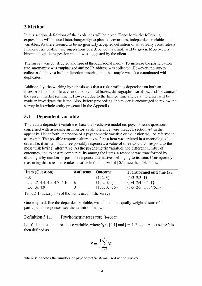
3 Method In this section, definitions of the explanans will be given. Henceforth, the following expressions will be used interchangeably: explanans, covariates, independent variables and variables. As there seemed to be no generally accepted definition of what really constitutes a financial risk profile, two suggestions of a dependent variable will be given. Moreover, a binomial logistic regression model was suggested by the client. The survey was constructed and spread through social media. To increase the participation rate, anonymity was emphasized and no IP-address was collected. However, the survey collector did have a built in function ensuring that the sample wasn’t contaminated with duplicates. Additionally, the working hypothesis was that a risk-profile is dependent on both an investor’s financial literacy level, behavioural biases, demographic variables, and “of course” the current market sentiment. However, due to the limited time and data, no effort will be made to investigate the latter. Also, before proceeding, the reader is encouraged to review the survey in its whole entity presented in the Appendix. 3.1 Dependent variable To create a dependent variable to base the predictive model on, psychometric questions concerned with assessing an investor’s risk tolerance were used, cf. section A4 in the appendix. Henceforth, the notion of a psychometric variable or a question will be referred to as an item. The possible response alternatives for an item was ordered in a chronological order. I.e. if an item had three possibly responses, a value of three would correspond to the most “risk loving” alternative. As the psychometric variables had different number of outcomes, and to ensure comparability among the items, a response was transformed by dividing it by number of possible response alternatives belonging to its item. Consequently, reassuring that a response takes a value in the interval of [0,1], see the table below. Item (Question) # of items Outcome Transformed outcome (ÆØ) 4.8 1

6 {1, 2, 3} {1/3, 2/3, 1}

4.1, 4.2, 4.4, 4.5, 4.7, 4.10 {1, 2, 3, 4} {1/4, 2/4, 3/4, 1} 4.3, 4.6, 4.9 3 {1, 2, 3, 4, 5} {1/5, 2/5, 3/5, 4/5,1}

Table 3.1: description of the items used in the survey One way to define the dependent variable, was to take the equally weighted sum of a participant’s responses, see the definition below. Definition 3.1.1 Psychometric test score (t-score)

Let Y± denote an item response variable, where Y± ∈ 0,1 and j = 1, 2…, n. A test score Y is then defined as

Y = &1n

Y±

≥

±ZD

where [ denotes the number of psychometric items used in the survey.

! 15!

!

Another proposed response variable was defined by taking a hindsight approach. That is, the participant was asked the following: “compared to others, how do you rate your willingness to take financial risks?”. Following this statement, the participant could choose one of the following four response alternatives:

1)! Extremely low 2)! Low 3)! High 4)! Extremely high

Definition 3.1.2 Dependent variable II If one sees the response to question 4.1 as an ordinal random variable,

! ∈ ¶CóI¶´¶õH&õL¥, õL¥, ℎ>Nℎ, ¶CóI¶´¶õH&ℎ>Nℎ then a binary dependent variable, 0, can be defined in the following manner

>?&! ∈ ¶CóI¶´¶õH&õL¥, õL¥ , õ¶ó&0 = 0

>?&! ∈ ℎ>Nℎ, ¶CóI¶´¶õH&ℎ>Nℎ , õ¶ó&0 = 1 3.2 Explanans To create some mind map, the explanans can be divided into four sub classes: indicator-, categorical-, quantitative- and psychometric variables. We say that a variable is an indicator if it has two distinct outcomes, e.g. “failure” or “success”, “man” or “woman” etc. Furthermore, we say that a variable is a categorical one if it has more than two outcomes, or levels. Also, we say that an indicator and a categorical variable is a qualitative variable. A quantitative variable on the other hand is more continuous in nature, e.g. ‘pre-tax income’ and ‘costs’, as it can take on far many more outcomes than a categorical one. A psychometric variable one the other hand should be seen an ordinal one, as illustrated in table 3.1 above. 3.3 Indicator variables Using the survey, the following indicator variables could be constructed. Definition 3.3.1 Gender

Let ò = ?¶´™õ¶, i.e. the is a female, and define the indicator variable as follows

ô∂ ! = 1&if&!& ∈ ò0&if&X& ∉ A

! 16!

!

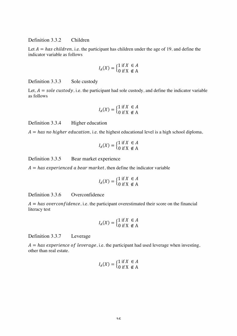
Definition 3.3.2 Children

Let ò = ℎ™î&Kℎ>õVI¶[, i.e. the participant has children under the age of 19, and define the indicator variable as follows

ô∂ ! = 1&if&!& ∈ ò0&if&X& ∉ A

Definition 3.3.3 Sole custody

Let, ò = îLõ¶&K®îóLVH, i.e. the participant had sole custody, and define the indicator variable as follows

ô∂ ! = 1&if&!& ∈ ò0&if&X& ∉ A

Definition 3.3.4 Higher education

ò = ℎ™î&[L&ℎ>Nℎ¶I&¶V®K™ó>L[, i.e. the highest educational level is a high school diploma,

ô∂ ! = 1&if&!& ∈ ò0&if&X& ∉ A

Definition 3.3.5 Bear market experience

ò = ℎ™î&¶Cc¶I>¶[K¶V&™&•¶™I&´™Ia¶ó, then define the indicator variable

ô∂ ! = 1&if&!& ∈ ò0&if&X& ∉ A

Definition 3.3.6 Overconfidence

ò = ℎ™î&LM¶IKL[?>V¶[K¶, i.e. the participant overestimated their score on the financial literacy test

ô∂ ! = 1&if&!& ∈ ò0&if&X& ∉ A

Definition 3.3.7 Leverage

ò = ℎ™î&¶Cc¶I>¶[K¶&L?&õ¶M¶I™N¶, i.e. the participant had used leverage when investing, other than real estate.

ô∂ ! = 1&if&!& ∈ ò0&if&X& ∉ A

! 17!

!

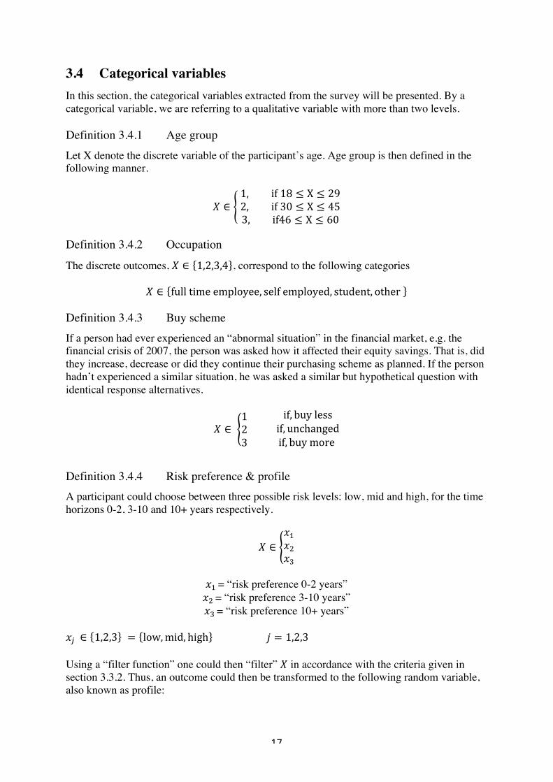
3.4 Categorical variables In this section, the categorical variables extracted from the survey will be presented. By a categorical variable, we are referring to a qualitative variable with more than two levels. Definition 3.4.1 Age group Let X denote the discrete variable of the participant’s age. Age group is then defined in the following manner.

! ∈&1, if&18 ≤ X ≤ 29&2, if&30 ≤ X ≤ 45&3, if46 ≤ X ≤ 60

Definition 3.4.2 Occupation

The discrete outcomes, ! ∈ 1,2,3,4 , correspond to the following categories

! ∈ full&time&employee, self&employed, student, other& Definition 3.4.3 Buy scheme If a person had ever experienced an “abnormal situation” in the financial market, e.g. the financial crisis of 2007, the person was asked how it affected their equity savings. That is, did they increase, decrease or did they continue their purchasing scheme as planned. If the person hadn’t experienced a similar situation, he was asked a similar but hypothetical question with identical response alternatives.

! ∈ &123&&&&&&&&&&&

if, buy&lessif, unchangedif, buy&more&

Definition 3.4.4 Risk preference & profile A participant could choose between three possible risk levels: low, mid and high, for the time horizons 0-2, 3-10 and 10+ years respectively.

! ∈CDCECº

CD&= “risk preference 0-2 years” CE&= “risk preference 3-10 years” Cº&= “risk preference 10+ years”

C\& ∈ 1,2,3 &= low,mid, high ^ = 1,2,3 Using a “filter function” one could then “filter” ! in accordance with the criteria given in section 3.3.2. Thus, an outcome could then be transformed to the following random variable, also known as profile:

! 18!

!

0 ∈ risk&avert, risk&neutral, risk&lover Moreover, by using the random variable !, that was just defined, one can create an additional variable 0, known as “profile”. To be more specific, a person is said to be risk avert if CD& = 1 and CE&, Cº& ∈ & 1,2 . If the following holds true, CD = 1, CE = 2 and Cº = 3, then a person is said to be risk neutral. Lastly, a profile known as risk lover can be defined as the combinatorics of preferred risk levels that were mutually exclusive with the other two profiles. Definition 3.4.5 Financial stamina We say that a person’s financial stamina describes their mental ability to recover from a financial loss. This trait will in turn be described in an ordinal manner by the variable below.

! ∈ 1,2,3,4 Where one represents that the person finds it very hard to recover, and vice versa for alternative four: they find it very ease. Definition 3.4.6 Financial literacy level In the survey, a financial literacy test consisting of five multiple choice questions were administered to the participants, cf. section A3 in the appendix. For each correct answer, the participant received a score of one. Thus, the participants could be grouped into three different groups.

•! If&the&participant&got&1&or&2&correct&answers, then&X = &1!•! If&the&participant&got&3&correct&answers, then&X = &2!•! If&the&participant&got&4&or&5&correct&answers, then&X = &2!

3.5 Quantitative variables In this section, the economic variables extracted from the survey will be presented. The purpose of normalizing some of the variables, i.e. to divide the outcome by some constant, was to establish a more coherent scale. Definition 3.6.1 Normalized income Normalized income was defined as the participant’s monthly income before taxes, divided by median pre-tax income in the city of Stockholm, Sweden, for the age group of 20-64 year olds, 31 575 SEK, (Statistik om Stockholm, 2015). Definition 3.6.2 Normalized cost In the same manner, normalized cost was defined as one’s living expenses divided by the median living expense in Sweden, 6 292 SEK, (Hushållens boendeutgift, 2015). Definition 3.6.3 Burn ratio Burn ratio was defined on a monthly basis, as the ratio between living expenses to income.

! 19!

!

Definition 3.6.4 Normalized wealth Normalized wealth was defined as the difference between assets and debt, divided by one’s wealth. Definition 3.6.5 Loan to value (LTV) ratio The LTV ratio was defined as one’s total debt to asset ratio. Definition 3.6.6 Asset class The survey participants were asked for their current asset allocation. The allocation, or portfolio weight, for four asset classes were asked for: equities, a risk free money market account (MMA), real estate, and other. If we let !\ denote the portfolio weight of the ^:th asset class, then the following holds:

!\ ∈ & 0, 1 , ^ = 1, 2, 3, 4 and by definition

!\ = 1ø

\ZD

Definition 3.6.7 Debt ratio By dividing one’s debt by their “monthly income”, we get a metric called “debt ratio”. 3.7 Psychometric variables The purpose of this section is to give a brief presentation of the psychometric variables. The intention of these variables were to measure the inherent ability of an individual’s willingness to take financial risk, a.k.a. risk tolerance. To do so, ten statements were put forward followed by some multiple choice alternatives, cf. section A4 in the Appendix. Naturally, the choice alternatives had an internal ranking order, presented in table 3.1 above, but which for the reader’s convenience will be re-iterated in table 3.2 below. Item (Question) # of items Outcome 4.10 1

6 {1, 2, 3}

4.1, 4.3, 4.5, 4.6, 4.9, 4.11 {1, 2, 3, 4} 4.4, 4.7, 4.10 3 {1, 2, 3, 4, 5}

Table 3.2: description of the items used in the survey

! 20!

!

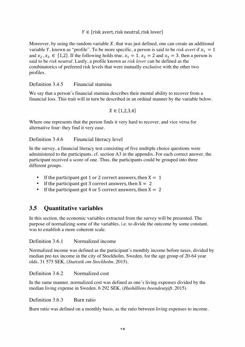
4 Data In this section, the main emphasis will be to give the reader some intuition of the data sample and its characteristics. The reason behind this approach, is the belief that it is quintessential to get an idea of the data sample before one can start the modelling process. Furthermore, as the client explicitly requested a grouping of each variable, the processes of doing so will also be presented. In total the authors received 110 different and individual responses for the full survey. 4.1 Quantitative data sample The purpose of this section is to get some intuition of the underlying probability distributions of the data sample. To do so, some descriptive statistics will be used. In some cases, the data sample was transformed by either taking the natural logarithm or squaring it. The purpose of doing so was to make it resemble that of a normal distributed variable. Below, two plots for each variable will be presented. In the upper end of each figure a scatter plot of the outcomes from the data sample will be plotted, and high leverage points will be highlighted in red. In the lower end of each figure, a QQ-plot of the pairwise points of the sample outcomes, and the corresponding quantiles of a normal distributed variable (fitted to the data sample) will be presented. To remove the potential influence of high leverage points, these were first removed, after which a sample mean was calculated and used as a replacement. Lastly, the term “logged” implies a usage of the natural logarithm. 4.1.1 QQ-plots and scatter plots

Figure 4.1: dependent variable (left) and normalized income (right) The dependent variable in figure 4.1 did neither take on any high leverage points, nor was it needed to be transformed in any way in order for it to resemble a normally distributed variable. By definition, this was also to be expected, cf. section 3.1. The data of normalized income was logged. Also, the reader notices that there is a cluster of outcomes in the left tail in the right hand figure. This was expected and was due to the “floor function”, c.f. definition 3.6.2. Moreover, the demographics of the writers is probably another reason for the clustering in the left tail.

! 21!

!

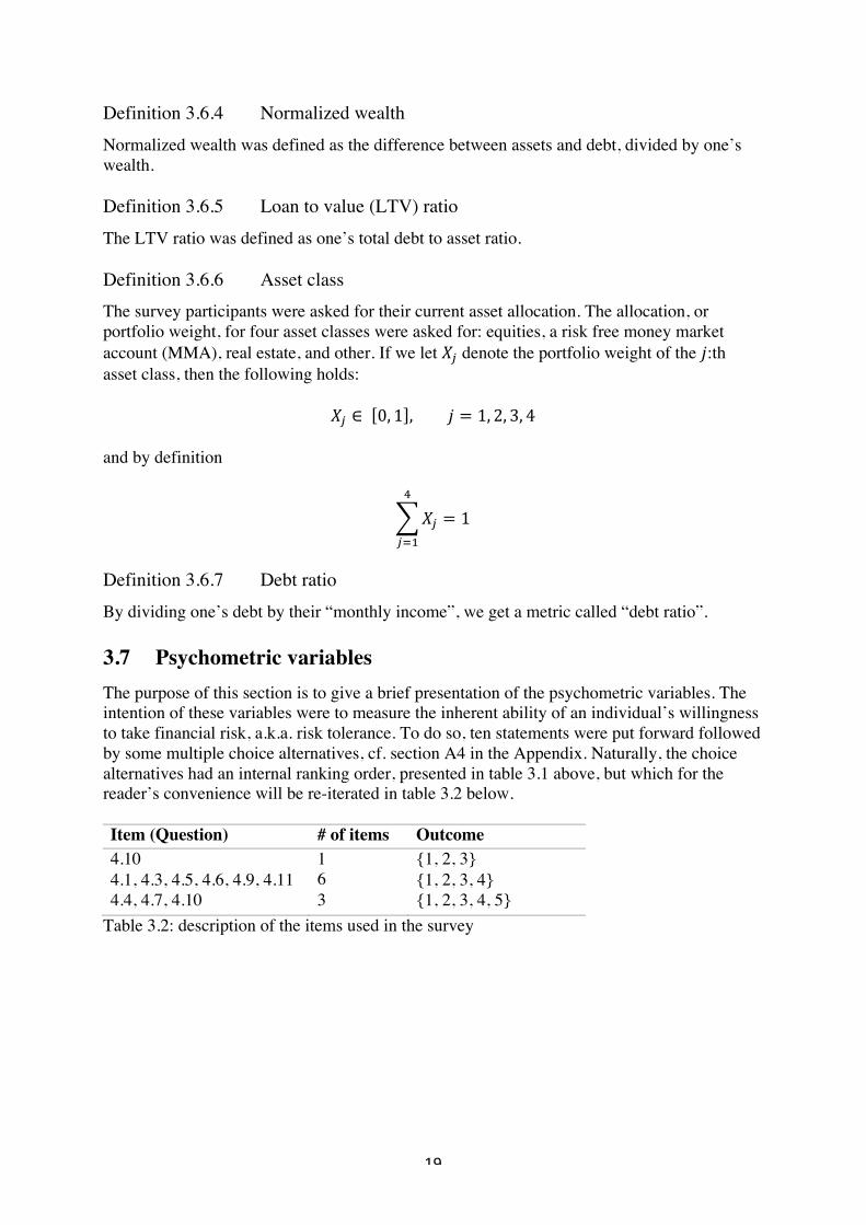
Figure 4.2: burn ratio (left) and normalized costs (right) The sample data of burn ratio was transformed by taking the square root. Likewise, the squared root was taken on the sample data of normalized costs. Also, there is a clustering in the left tail. This is due to an adjustment, cf. definition 3.6.3.

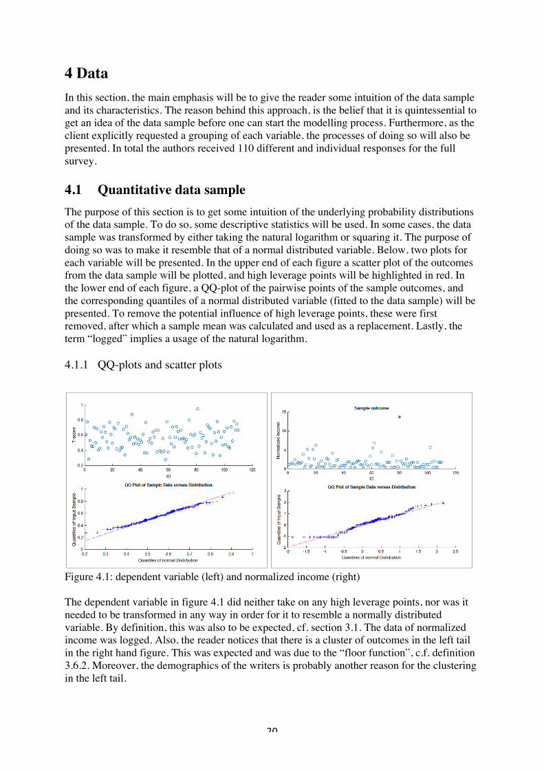
Figure 4.3: equity in portfolio % (left) and MMA in portfolio % (right) No transformation of the sample data of equity in portfolio % was considered to be needed. The sample of money market in portfolio % was logged. As around ten individuals had stated zero liquidity, i.e. a balance of zero in the money market account, these observations were set to 0.05 before taking the logarithm. It seems likely that these individuals had misinterpreted the question.

! 22!

!

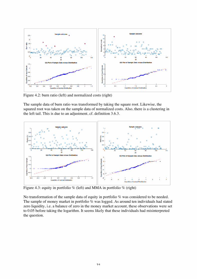
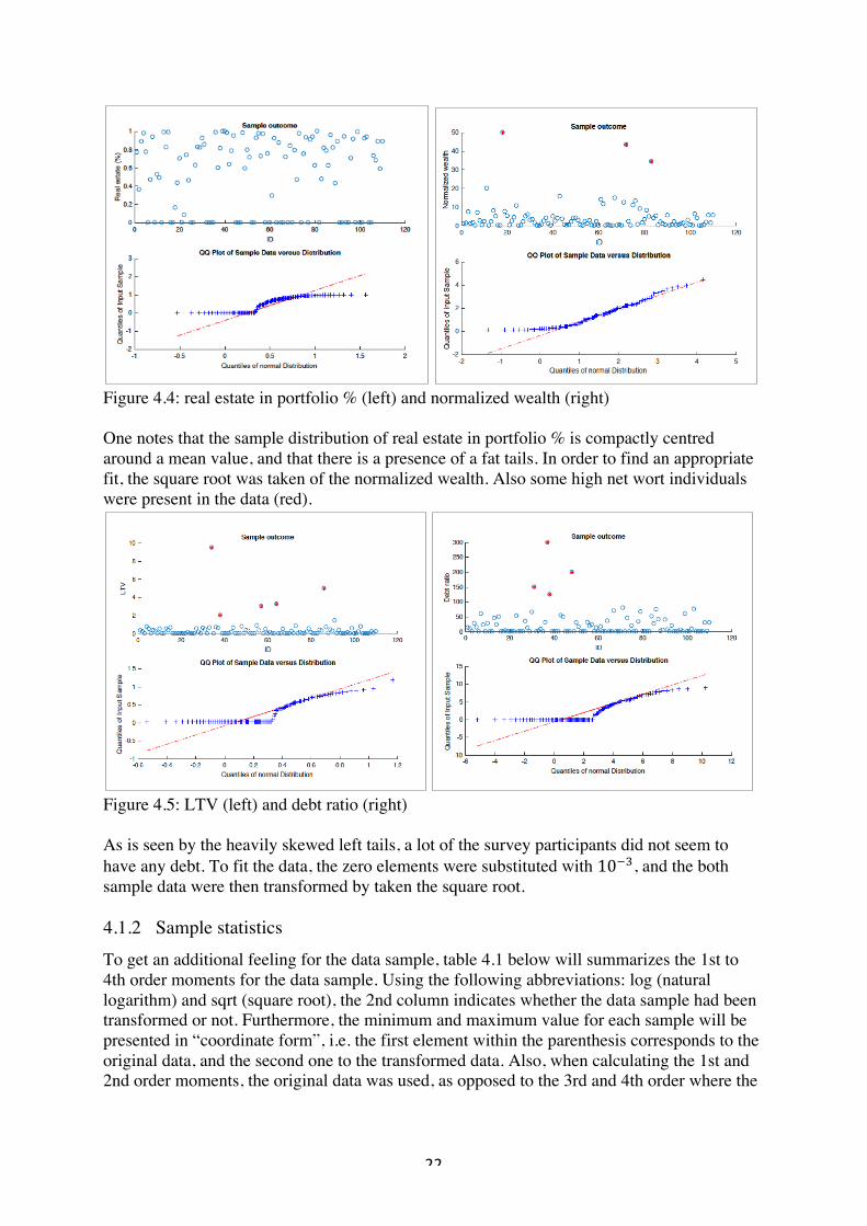
Figure 4.4: real estate in portfolio % (left) and normalized wealth (right) One notes that the sample distribution of real estate in portfolio % is compactly centred around a mean value, and that there is a presence of a fat tails. In order to find an appropriate fit, the square root was taken of the normalized wealth. Also some high net wort individuals were present in the data (red).

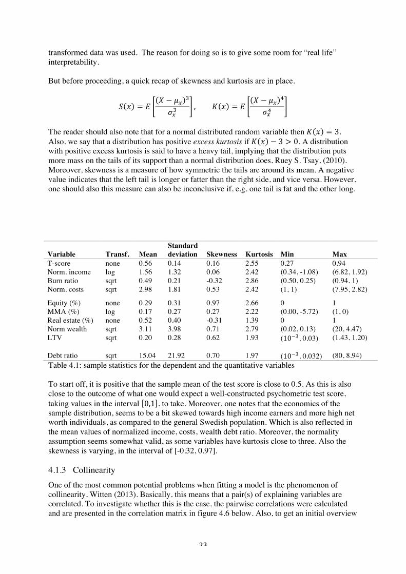
Figure 4.5: LTV (left) and debt ratio (right) As is seen by the heavily skewed left tails, a lot of the survey participants did not seem to have any debt. To fit the data, the zero elements were substituted with 10fº, and the both sample data were then transformed by taken the square root. 4.1.2 Sample statistics To get an additional feeling for the data sample, table 4.1 below will summarizes the 1st to 4th order moments for the data sample. Using the following abbreviations: log (natural logarithm) and sqrt (square root), the 2nd column indicates whether the data sample had been transformed or not. Furthermore, the minimum and maximum value for each sample will be presented in “coordinate form”, i.e. the first element within the parenthesis corresponds to the original data, and the second one to the transformed data. Also, when calculating the 1st and 2nd order moments, the original data was used, as opposed to the 3rd and 4th order where the

! 23!

!

transformed data was used. The reason for doing so is to give some room for “real life” interpretability. But before proceeding, a quick recap of skewness and kurtosis are in place.

~ C = �! − ¿¡ º

Q¡º, ` C = �

! − ¿¡ ø

Q¡ø

The reader should also note that for a normal distributed random variable then ` C = 3. Also, we say that a distribution has positive excess kurtosis if ` C − 3 > 0. A distribution with positive excess kurtosis is said to have a heavy tail, implying that the distribution puts more mass on the tails of its support than a normal distribution does, Ruey S. Tsay, (2010). Moreover, skewness is a measure of how symmetric the tails are around its mean. A negative value indicates that the left tail is longer or fatter than the right side, and vice versa. However, one should also this measure can also be inconclusive if, e.g. one tail is fat and the other long.

Variable Transf. Mean Standard deviation Skewness Kurtosis Min Max

T-score none 0.56 0.14 0.16 2.55 0.27 0.94 Norm. income log 1.56 1.32 0.06 2.42 (0.34, -1.08) (6.82, 1.92) Burn ratio sqrt 0.49 0.21 -0.32 2.86 (0.50, 0.25) (0.94, 1) Norm. costs sqrt 2.98 1.81 0.53 2.42 (1, 1) (7.95, 2.82)

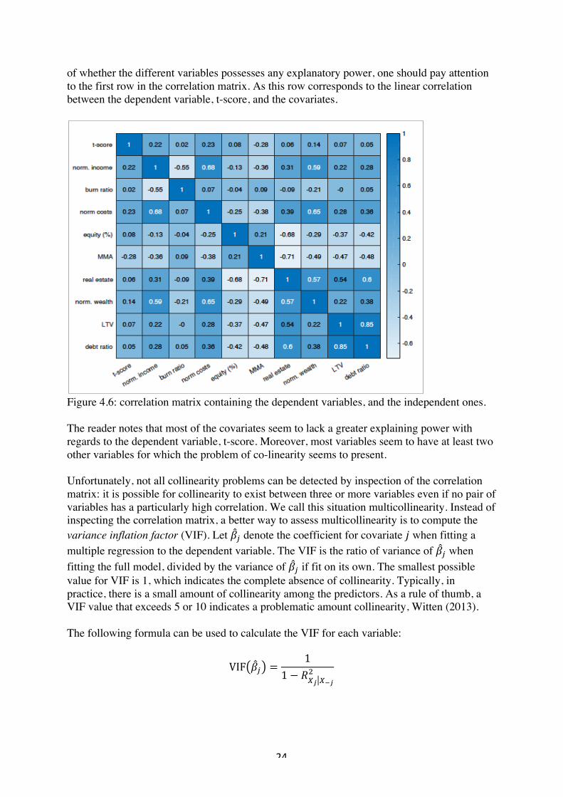
Equity (%) none 0.29 0.31 0.97 2.66 0 1 MMA (%) log 0.17 0.27 0.27 2.22 (0.00, -5.72) (1, 0) Real estate (%) none 0.52 0.40 -0.31 1.39 0 1 Norm wealth sqrt 3.11 3.98 0.71 2.79 (0.02, 0.13) (20, 4.47) LTV sqrt 0.20 0.28 0.62 1.93 (10fº, 0.03) (1.43, 1.20) Debt ratio sqrt 15.04 21.92 0.70 1.97 (10fº, 0.032) (80, 8.94) Table 4.1: sample statistics for the dependent and the quantitative variables To start off, it is positive that the sample mean of the test score is close to 0.5. As this is also close to the outcome of what one would expect a well-constructed psychometric test score, taking values in the interval 0,1 , to take. Moreover, one notes that the economics of the sample distribution, seems to be a bit skewed towards high income earners and more high net worth individuals, as compared to the general Swedish population. Which is also reflected in the mean values of normalized income, costs, wealth debt ratio. Moreover, the normality assumption seems somewhat valid, as some variables have kurtosis close to three. Also the skewness is varying, in the interval of [-0.32, 0.97]. 4.1.3 Collinearity One of the most common potential problems when fitting a model is the phenomenon of collinearity, Witten (2013). Basically, this means that a pair(s) of explaining variables are correlated. To investigate whether this is the case, the pairwise correlations were calculated and are presented in the correlation matrix in figure 4.6 below. Also, to get an initial overview

! 24!

!

of whether the different variables possesses any explanatory power, one should pay attention to the first row in the correlation matrix. As this row corresponds to the linear correlation between the dependent variable, t-score, and the covariates.

Figure 4.6: correlation matrix containing the dependent variables, and the independent ones. The reader notes that most of the covariates seem to lack a greater explaining power with regards to the dependent variable, t-score. Moreover, most variables seem to have at least two other variables for which the problem of co-linearity seems to present. Unfortunately, not all collinearity problems can be detected by inspection of the correlation matrix: it is possible for collinearity to exist between three or more variables even if no pair of variables has a particularly high correlation. We call this situation multicollinearity. Instead of inspecting the correlation matrix, a better way to assess multicollinearity is to compute the variance inflation factor (VIF). Let n\ denote the coefficient for covariate ^ when fitting a multiple regression to the dependent variable. The VIF is the ratio of variance of n\ when fitting the full model, divided by the variance of n\ if fit on its own. The smallest possible value for VIF is 1, which indicates the complete absence of collinearity. Typically, in practice, there is a small amount of collinearity among the predictors. As a rule of thumb, a VIF value that exceeds 5 or 10 indicates a problematic amount collinearity, Witten (2013). The following formula can be used to calculate the VIF for each variable:

VIF n\ =1

1 − úOƒ O≈ƒE

! 25!

!

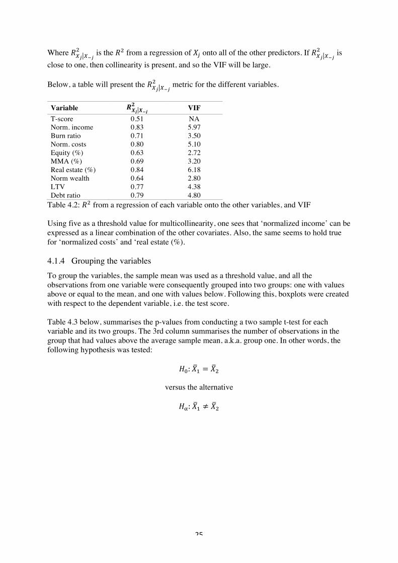
Where úOƒ O≈ƒE is the úE from a regression of !\ onto all of the other predictors. If úOƒ O≈ƒ

E is close to one, then collinearity is present, and so the VIF will be large. Below, a table will present the úOƒ O≈ƒ

E metric for the different variables. Variable ∆iØ i≈Ø

« VIF T-score 0.51 NA Norm. income 0.83 5.97 Burn ratio 0.71 3.50 Norm. costs 0.80 5.10 Equity (%) 0.63 2.72 MMA (%) 0.69 3.20 Real estate (%) 0.84 6.18 Norm wealth 0.64 2.80 LTV 0.77 4.38 Debt ratio 0.79 4.80

Table 4.2: úE from a regression of each variable onto the other variables, and VIF Using five as a threshold value for multicollinearity, one sees that ‘normalized income’ can be expressed as a linear combination of the other covariates. Also, the same seems to hold true for ‘normalized costs’ and ‘real estate (%). 4.1.4 Grouping the variables To group the variables, the sample mean was used as a threshold value, and all the observations from one variable were consequently grouped into two groups: one with values above or equal to the mean, and one with values below. Following this, boxplots were created with respect to the dependent variable, i.e. the test score. Table 4.3 below, summarises the p-values from conducting a two sample t-test for each variable and its two groups. The 3rd column summarises the number of observations in the group that had values above the average sample mean, a.k.a. group one. In other words, the following hypothesis was tested:

Äo:&!D = !E

versus the alternative

Ä»:&!D ≠ !E

! 26!

!

Variable p-value #obs. in group 1 Norm. income 0.037 * 61 Burn ratio 0.281 61 Norm. costs 0.268 51 Equity (%) 0.602 39 MMA (%) 0.004 ** 48 Real estate (%) 0.928 63 Norm wealth 0.202 55 LTV 0.472 52 Debt ratio 0.259 48

Table 4.3: p-value from two sample t-test, and number of observations in group 1. According to Olsson (2002), the conventional 5% significance level is often too strict for model building purposes. A significance level in the range 15-25% may be used instead. From table 4.3, one can identify three variables that clearly do not obey this rule: ‘equity in portfolio (%)’, ‘real estate in portfolio (%)’ and ‘LTV’. To investigate whether this was due to the initial threshold value of the sample mean, the three variables were grouped by using another grouping technique. More specifically, the following method was used for the three insignificant variables of ‘equity in portfolio (%)’, ‘real estate in portfolio (%)’ and ‘LTV’,

i)! if&…O C ≤ 1/3,! then&DD = &1,! otherwise&DD = &0!!

ii)! if&1/3 < …O C < 2/3,! then&DE = &1,! otherwise&DE = &0! where !~s ¿, QE In other words, the inverse of the normal cumulative distribution function, with sample mean and standard error were used as input. Thus, the following regression was made to investigate whether the new grouping technique made any difference:

H = no + nD&DD + nE&DE + À where H corresponds to the psychometric test score, definition 3.1.1. By doing so, an F-test was used to test the following null hypothesis,

Äo ∶ &nD = nE = 0

versus the alternative

ÄÖ ∶ &at&least&one&β±&is&non-zero The result of these F-tests are presented in table 4.4 below.

! 27!

!

Variable p-value Equity (%) 0.645 Real estate (%) 0.096 LTV 0.410

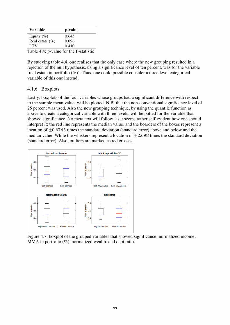
Table 4.4: p-value for the F-statistic By studying table 4.4, one realises that the only case where the new grouping resulted in a rejection of the null hypothesis, using a significance level of ten percent, was for the variable ‘real estate in portfolio (%)’. Thus, one could possible consider a three level categorical variable of this one instead. 4.1.6 Boxplots Lastly, boxplots of the four variables whose groups had a significant difference with respect to the sample mean value, will be plotted. N.B. that the non-conventional significance level of 25 percent was used. Also the new grouping technique, by using the quantile function as above to create a categorical variable with three levels, will be potted for the variable that showed significance. No meta text will follow, as it seems rather self-evident how one should interpret it: the red line represents the median value, and the boarders of the boxes represent a location of ±0.6745 times the standard deviation (standard error) above and below and the median value. While the whiskers represent a location of ±2.698 times the standard deviation (standard error). Also, outliers are marked as red crosses.

Figure 4.7: boxplot of the grouped variables that showed significance: normalized income, MMA in portfolio (%), normalized wealth, and debt ratio.

! 28!

!

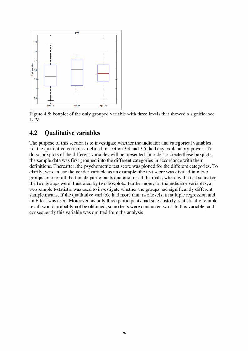
Figure 4.8: boxplot of the only grouped variable with three levels that showed a significance LTV 4.2 Qualitative variables The purpose of this section is to investigate whether the indicator and categorical variables, i.e. the qualitative variables, defined in section 3.4 and 3.5, had any explanatory power. To do so boxplots of the different variables will be presented. In order to create these boxplots, the sample data was first grouped into the different categories in accordance with their definitions. Thereafter, the psychometric test score was plotted for the different categories. To clarify, we can use the gender variable as an example: the test score was divided into two groups, one for all the female participants and one for all the male, whereby the test score for the two groups were illustrated by two boxplots. Furthermore, for the indicator variables, a two sample t-statistic was used to investigate whether the groups had significantly different sample means. If the qualitative variable had more than two levels, a multiple regression and an F-test was used. Moreover, as only three participants had sole custody, statistically reliable result would probably not be obtained, so no tests were conducted w.r.t. to this variable, and consequently this variable was omitted from the analysis.

! 29!

!

4.2.1 Two sample t-test To determine whether the indicator variables, i.e. variables with only two outcomes, had any explanatory power, a two sample t-test was conducted. The result from doing so will be presented in table 4.5 below. Note that there were 110 participants in total, and in all cases 108 degrees of freedom were used.

Indicator variable p-value Distribution of outcomes Gender 0.000 *** 72 males Children 0.007 ** 33 had children Higher education 0.195 12 had no university degree Bear market experience 0.000 *** 47 had experienced a bear market

Overconfidence bias 0.608 31 were overconfident Leverage 0.000 *** 26 had experience of leverage investing

Table 4.5: p-value for the two sample t-test Thus, by using an Ç-significance level of 5 percent, all but the higher education- and the overconfidence indicator seemed to possess any discriminant power. Especially positive were the result for gender, bear market experience, and experience of financial leverage. 4.2.2 F-test To assesses whether the categorical variables, having more than two levels, had any discriminatory power, a multiple regression and an F-test were used. I.e. using the following notations

H = no + nD&DD +&…&+&nñfD&DŒfD + À Where &D± represents a dummy variable for level ^, c is the number of levels for the qualitative variables, and y is the dependent variable of test score, the following null hypothesis can be tested:

Äo ∶ &nD = nE = &… &= nñfD = 0

versus the alternative

ÄÖ ∶ &at&least&one&β±&is&nonœzero Below a table summarizes the p-value for the F-statistic when conducting the hypotheses testing.

! 30!

!

Categorical variable p-value Distribution of outcomes Age group 0.008 ** 18-29 (60), 30-45 (25), 46-60 (21) Occupation 0.009 ** employee (60), entrepreneur (19), student (24), other (7) Risk preference 0-2 years 0.878 low (37), mid (49), high (24) Risk preference 3-10 years 0.000 *** low (21), mid (68), high (21)

Risk preference 10+ years 0.000 *** low (41), mid (28), high (41) Profile 0.011 ** risk avert (15), risk neutral (16), risk taker (79) Buy scheme 0.000 *** buy less (19), hold (70), buy more (21) Financial literacy level 0.000 *** low (17), mid (19), high (74) Financial stamina 0.000 *** very hard (8), hard (32), easy (63), very easy (7)

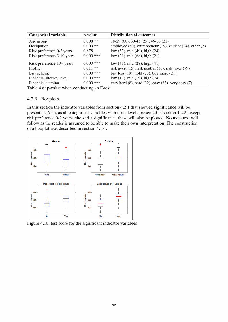
Table 4.6: p-value when conducting an F-test 4.2.3 Boxplots In this section the indicator variables from section 4.2.1 that showed significance will be presented. Also, as all categorical variables with three levels presented in section 4.2.2, except risk preference 0-2 years, showed a significance, these will also be plotted. No meta text will follow as the reader is assumed to be able to make their own interpretation. The construction of a boxplot was described in section 4.1.6.

Figure 4.10: test score for the significant indicator variables

! 31!

!

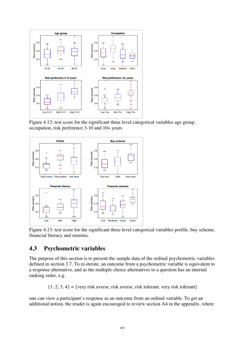
Figure 4.12: test score for the significant three level categorical variables age group, occupation, risk preference 3-10 and 10+ years

Figure 4.13: test score for the significant three level categorical variables profile, buy scheme, financial literacy and stamina. 4.3 Psychometric variables

The purpose of this section is to present the sample data of the ordinal psychometric variables defined in section 3.7. To re-iterate, an outcome from a psychometric variable is equivalent to a response alternative, and as the multiple choice alternatives to a question has an internal ranking order, e.g.

{1, 2, 3, 4} = {very risk averse, risk averse, risk tolerant, very risk tolerant} one can view a participant’s response as an outcome from an ordinal variable. To get an additional notion, the reader is again encouraged to review section A4 in the appendix, where

! 32!

!

all psychometric questions and responses are stated. Moreover, by considering the number of outcomes, one can divide the ordinal variables into three different sub-categories.

Outcome Number of questions

{1,2,3} 1

{1,2,3,4} 6

{1,2,3,4,5} 3

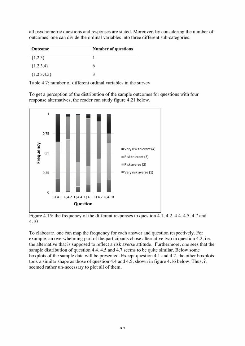
Table 4.7: number of different ordinal variables in the survey To get a perception of the distribution of the sample outcomes for questions with four response alternatives, the reader can study figure 4.21 below.

Figure 4.15: the frequency of the different responses to question 4.1, 4.2, 4.4, 4.5, 4.7 and 4.10 To elaborate, one can map the frequency for each answer and question respectively. For example, an overwhelming part of the participants chose alternative two in question 4.2, i.e. the alternative that is supposed to reflect a risk averse attitude. Furthermore, one sees that the sample distribution of question 4.4, 4.5 and 4.7 seems to be quite similar. Below some boxplots of the sample data will be presented. Except question 4.1 and 4.2, the other boxplots took a similar shape as those of question 4.4 and 4.5, shown in figure 4.16 below. Thus, it seemed rather un-necessary to plot all of them.

0

0,25

0,5

0,75

1

Q!4.1 Q!4.2 Q!4.4 Q!4.5 Q!4.7 Q!4.10

Freq

uency

Question

Very!risk!tolerant!(4)

Risk!tolerant!(3)

Risk!averse!(2)

Very!risk!averse!(1)

! 33!

!

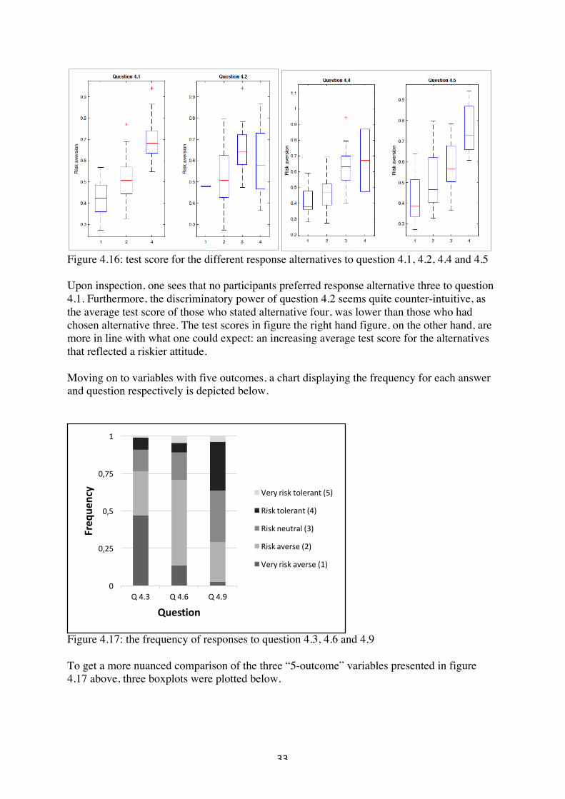
Figure 4.16: test score for the different response alternatives to question 4.1, 4.2, 4.4 and 4.5 Upon inspection, one sees that no participants preferred response alternative three to question 4.1. Furthermore, the discriminatory power of question 4.2 seems quite counter-intuitive, as the average test score of those who stated alternative four, was lower than those who had chosen alternative three. The test scores in figure the right hand figure, on the other hand, are more in line with what one could expect: an increasing average test score for the alternatives that reflected a riskier attitude. Moving on to variables with five outcomes, a chart displaying the frequency for each answer and question respectively is depicted below.

Figure 4.17: the frequency of responses to question 4.3, 4.6 and 4.9 To get a more nuanced comparison of the three “5-outcome” variables presented in figure 4.17 above, three boxplots were plotted below.

0

0,25

0,5

0,75

1

Q!4.3 Q!4.6 Q!4.9

Freq

uency

Question

Very!risk!tolerant!(5)

Risk!tolerant!(4)

Risk!neutral!(3)

Risk!averse!(2)

Very!risk!averse!(1)

! 34!

!

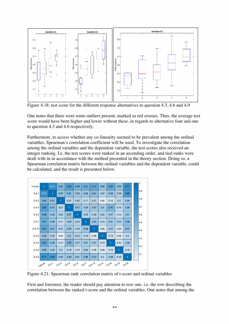
Figure 4.18: test score for the different response alternatives to question 4.3, 4.6 and 4.9 One notes that there were some outliers present, marked as red crosses. Thus, the average test score would have been higher and lower without these, in regards to alternative four and one to question 4.3 and 4.6 respectively. Furthermore, to access whether any co-linearity seemed to be prevalent among the ordinal variables, Spearman’s correlation coefficient will be used. To investigate the correlation among the ordinal variables and the dependent variable, the test scores also received an integer ranking. I.e. the test scores were ranked in an ascending order, and tied ranks were dealt with in in accordance with the method presented in the theory section. Doing so, a Spearman correlation matrix between the ordinal variables and the dependent variable, could be calculated, and the result is presented below.

Figure 4.21: Spearman rank correlation matrix of t-score and ordinal variables First and foremost, the reader should pay attention to row one, i.e. the row describing the correlation between the ranked t-score and the ordinal variables. One notes that among the

! 35!

!

four-outcome ordinal variables (Q4.1, 4.2, 4.4, 4.5, 4.7, 4.10), then the ordinal variable constructed from question 4.1 has the highest correlation with the test score. Also, three-outcome variable (Q 4.8) also has a quite high correlation with the response. Overall, it seems apparent that the ordinal variables, have a better explanatory power, compared to the quantitative ones. Moreover, also note that the ordinal variables seem to have an ingredient of collinearity.

! 36!

!

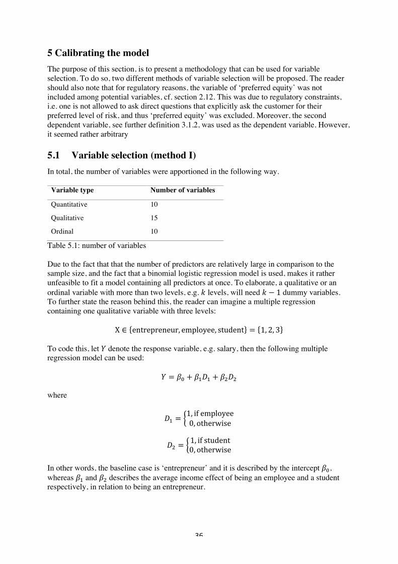
5 Calibrating the model The purpose of this section, is to present a methodology that can be used for variable selection. To do so, two different methods of variable selection will be proposed. The reader should also note that for regulatory reasons, the variable of ‘preferred equity’ was not included among potential variables, cf. section 2.12. This was due to regulatory constraints, i.e. one is not allowed to ask direct questions that explicitly ask the customer for their preferred level of risk, and thus ‘preferred equity’ was excluded. Moreover, the second dependent variable, see further definition 3.1.2, was used as the dependent variable. However, it seemed rather arbitrary 5.1 Variable selection (method I) In total, the number of variables were apportioned in the following way.

Variable type Number of variables

Quantitative 10

Qualitative 15

Ordinal 10

Table 5.1: number of variables Due to the fact that that the number of predictors are relatively large in comparison to the sample size, and the fact that a binomial logistic regression model is used, makes it rather unfeasible to fit a model containing all predictors at once. To elaborate, a qualitative or an ordinal variable with more than two levels, e.g. a levels, will need a − 1 dummy variables. To further state the reason behind this, the reader can imagine a multiple regression containing one qualitative variable with three levels:

X ∈ entrepreneur, employee, student = 1, 2, 3 To code this, let 0 denote the response variable, e.g. salary, then the following multiple regression model can be used:

0 = no + nD—D + nE—E where

—D =1, if&employee0, otherwise

—E =1, if&student0, otherwise

In other words, the baseline case is ‘entrepreneur’ and it is described by the intercept no, whereas nD and nE describes the average income effect of being an employee and a student respectively, in relation to being an entrepreneur.

! 37!

!

Thus if one would use the coding technique presented above, there would be a total of 68 dummy variables, consequently making the estimates highly unstable – as there were only 110 observations in total. However, using the technique of transforming the ordinal variables with four- and five outcomes into ones with two and three outcomes (levels) respectively, as presented in section 2.1.1, one can reduce the number of dummy variables needed to depict the ordinal variables, from 32 to 14. Despite this, there would still be a total of 50 dummy variables. Therefore, the procedure of variable selection was divided into four separate stages:

i)! select the most promising quantitative variables ii)! select the most promising qualitative variables iii)! select the most promising ordinal variables iv)! use the variables from step i-iii to make a final variable selection

By doing so, one assures that there would be at most 27 dummy variables – in the case of the qualitative variables, in step two. Furthermore, the algorithm of ‘forward stepwise selection’, presented in section 2.8 was used to select variables. The criteria used in the iterative algorithm of forward stepwise selection, was to pick out variables that passed a specific Ç-significance level, in terms of the likelihood-ratio chi-square test. Accordingly, a presentation of the procedures outlined in step 1-4 will follow.

5.1.1 Subset selection – quantitative variables As mentioned in section 4.1, the quantitative variables were transformed into indicator variables by separating each data sample into two groups: one containing observations with values above or equal to the sample mean, and vice versa. By first setting the specific Ç-significance level to 5 percent, two variables were picked out: ‘normalized income’ and ‘burn ratio’. But as mentioned in Olsson, Ulf (2002), it is customary to extended the significance level to a more tolerant one. Thus, the algorithm was run again, but now with an Ç-significance level set to 20 percent. However, this resulted in the same variable selection as before. Thus the following two dummy variables were chosen:

—D =1,&income was higher than sample average&

0, otherwise&

—E =1,&burn ratio was higher than sample average&

0, otherwise& To get some notion of how this reduced model performed against the full model, i.e. the one containing all of the ten quantitative indicator variables, the re-sampling method of leave-one-out cross-validation was used to approximate the accuracy ratio. Furthermore, the Akaike information criterion (AIC) was also calculated for the two model. Also, the three metrics were calculated for the model that only contained an intercept term, i.e. a model that contained no predictors.

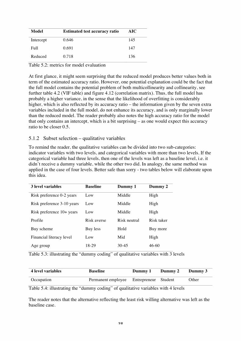
! 38!

!

Model Estimated test accuracy ratio AIC

Intercept 0.646 145

Full 0.691 147

Reduced 0.718 136

Table 5.2: metrics for model evaluation At first glance, it might seem surprising that the reduced model produces better values both in term of the estimated accuracy ratio. However, one potential explanation could be the fact that the full model contains the potential problem of both multicollinearity and collinearity, see further table 4.2 (VIF table) and figure 4.12 (correlation matrix). Thus, the full model has probably a higher variance, in the sense that the likelihood of overfitting is considerably higher, which is also reflected by its accuracy ratio – the information given by the seven extra variables included in the full model, do not enhance its accuracy, and is only marginally lower than the reduced model. The reader probably also notes the high accuracy ratio for the model that only contains an intercept, which is a bit surprising – as one would expect this accuracy ratio to be closer 0.5. 5.1.2 Subset selection – qualitative variables To remind the reader, the qualitative variables can be divided into two sub-categories: indicator variables with two levels, and categorical variables with more than two levels. If the categorical variable had three levels, then one of the levels was left as a baseline level, i.e. it didn’t receive a dummy variable, while the other two did. In analogy, the same method was applied in the case of four levels. Better safe than sorry - two tables below will elaborate upon this idea.

3 level variables Baseline Dummy 1 Dummy 2

Risk preference 0-2 years Low Middle High

Risk preference 3-10 years Low Middle High

Risk preference 10+ years Low Middle High

Profile Risk averse Risk neutral Risk taker

Buy scheme Buy less Hold Buy more

Financial literacy level Low Mid High

Age group 18-29 30-45 46-60

Table 5.3: illustrating the “dummy coding” of qualitative variables with 3 levels

4 level variables Baseline Dummy 1 Dummy 2 Dummy 3

Occupation Permanent employee Entrepreneur Student Other

Table 5.4: illustrating the “dummy coding” of qualitative variables with 4 levels The reader notes that the alternative reflecting the least risk willing alternative was left as the baseline case.

! 39!

!

Moreover, as there were only eight and seven participants that had stated it to be “very hard” and “very easy” to recover from a financial loss, these two categories were merged with the “hard” and the “easy” categories respectively. Thus, by following the instruction above, a total of 24 dummy variables corresponding to different levels within the qualitative variables, were constructed. And by preceding as in the previous section, one could again use the approach of a ‘forward subset selection’ with an Ç-significance level of 5 percent. Following this, the variable selection algorithm stated that the following dummy variables should be included:

—D =1,&had experienced a bear market&

0, otherwise&

—E =1, preferred&mid&risk&level&10 + &years

0, otherwise&

—º =1, preferred&high&risk&level&10 + &years

0, otherwise&

—ø =1,would&stick&to&a&′buy&scheme′&in&a&bear&market

0, otherwise& Before continuing, a short reflection is in place. From an intuitive point of view, the variable selection seems natural. In the sense that all selected dummy variables reflect a multiple choice alternative, that suggests that the investor is either experienced, would take rational decisions in a bear market (buy more), cf. Graham, B. (2006), and would prefer a mid to high risk level. In the same manner as before, the reduced model was benchmarked with the full model containing all qualitative predictors, and the one containing the intercept term.

Model Estimated test accuracy ratio AIC

Intercept 0.646 145

Full 0.691 115

Reduced 0.846 96

Table 5.5: metrics for model evaluation As in the previous section, we see that the reduced model performs better, both in terms of AIC and its estimated test accuracy ratio. The reason to this is probably the same as before: co- and multicollinearity. This thesis was also somewhat confirmed when fitting the full model, as Matlab’s built-in function that was used to estimate the model parameters (fitglm), threw the following warning: “The estimated coefficients perfectly separate failures from successes”. Put differently: the predictors are either collinear or one predictor(s) can be expressed as linear combination of three or more variables (multicollinearity). Moreover,

! 40!

!

worth noting is also that when comparing the qualitative variables vis-à-vis with the quantitative indicator variables, the former seems possess better predictor power. 5.1.3 Subset selection – ordinal variables Before proceeding with the variable selection, the ordinal variables were transformed in accordance with the technique presented in section 2.1, i.e. variables with five and four outcomes were transformed into ones with three and two outcomes respectively. Besides this, as was indicated by the “adjusted” Spearman correlation matrix in figure 4.31, it seems apparent that there is some presence of co-linearity among the ordinal variables. This was also confirmed when fitting the full model containing all ordinal variables, as Matlab threw an error message indicating the presence of co- and or multicollinearity. To avoid the presence of this, the subset selection was conducted in the following way:

i)! Perform subset selection on ordinal variables with two outcomes ii)! Perform subset selection on ordinal variables with three outcomes iii)! Perform subset selection using the variables from i-ii

Moreover, when using an Ç-significance level of five percent, the number of suggested variables were quite great, i.e. the intention of reducing the number of variables was not fulfilled. Therefore, the Ç-significance was instead set to one percent. Following this, the following “two-outcome” variables were suggested:

—D =1,&answer at Q 4.2 corresponded to "mid-" or "high risk preference"

0, otherwise&

—E =1,&answer at Q 4.4 corresponded to "mid-" or "high risk preference"

0, otherwise& Moreover, using the coding scheme presented at the beginning of section five for variables having more than two levels, the following dummy variables were suggested among the three level ordinal variables:

—º =1,&answer at Q 4.3 corresponded to "high risk preference"

0, otherwise&

—ø =1,&answer at Q 4.9 corresponded to "mid risk preference"

0, otherwise&

—” =1,&answer at Q 4.9 corresponded to "high risk preference"

0, otherwise& Next, step three as outlined above was conducted, i.e. the sub selection algorithm was again run on the dummy variables —D to —”, resulting in a final selection of the dummy variables —º, —ø and —”. In other words, none of the “two-outcome” ordinal variables were selected. Below is a table comparing the full, reduced and the intercept model. In this setting, the “full model” is referring to the one where all ordinal variables were included, and the reduced to the one containing the final subset selection of variables —º, —ø and —”.

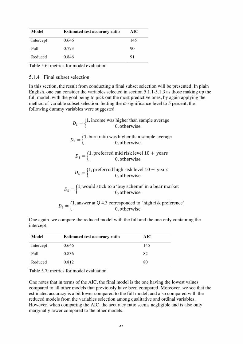
! 41!

!

Model Estimated test accuracy ratio AIC

Intercept 0.646 145

Full 0.773 90

Reduced 0.846 91

Table 5.6: metrics for model evaluation 5.1.4 Final subset selection In this section, the result from conducting a final subset selection will be presented. In plain English, one can consider the variables selected in section 5.1.1-5.1.3 as those making up the full model, with the goal being to pick out the most predictive ones, by again applying the method of variable subset selection. Setting the Ç-significance level to 5 percent, the following dummy variables were suggested

—D =1,&income was higher than sample average&

0, otherwise&

—E =1,&burn ratio was higher than sample average&

0, otherwise&

—º =1, preferred&mid&risk&level&10 + &years

0, otherwise&

—ø =1, preferred&high&risk&level&10 + &years

0, otherwise&

—” =1,would&stick&to&a&′buy&scheme′&in&a&bear&market

0, otherwise&

—‘ =1,&answer at Q 4.3 corresponded to "high risk preference"

0, otherwise& One again, we compare the reduced model with the full and the one only containing the intercept.

Model Estimated test accuracy ratio AIC

Intercept 0.646 145

Full 0.836 82

Reduced 0.812 80

Table 5.7: metrics for model evaluation One notes that in terms of the AIC, the final model is the one having the lowest values compared to all other models that previously have been compared. Moreover, we see that the estimated accuracy is a bit lower compared to the full model, and also compared with the reduced models from the variables selection among qualitative and ordinal variables. However, when comparing the AIC, the accuracy ratio seems negligible and is also only marginally lower compared to the other models.

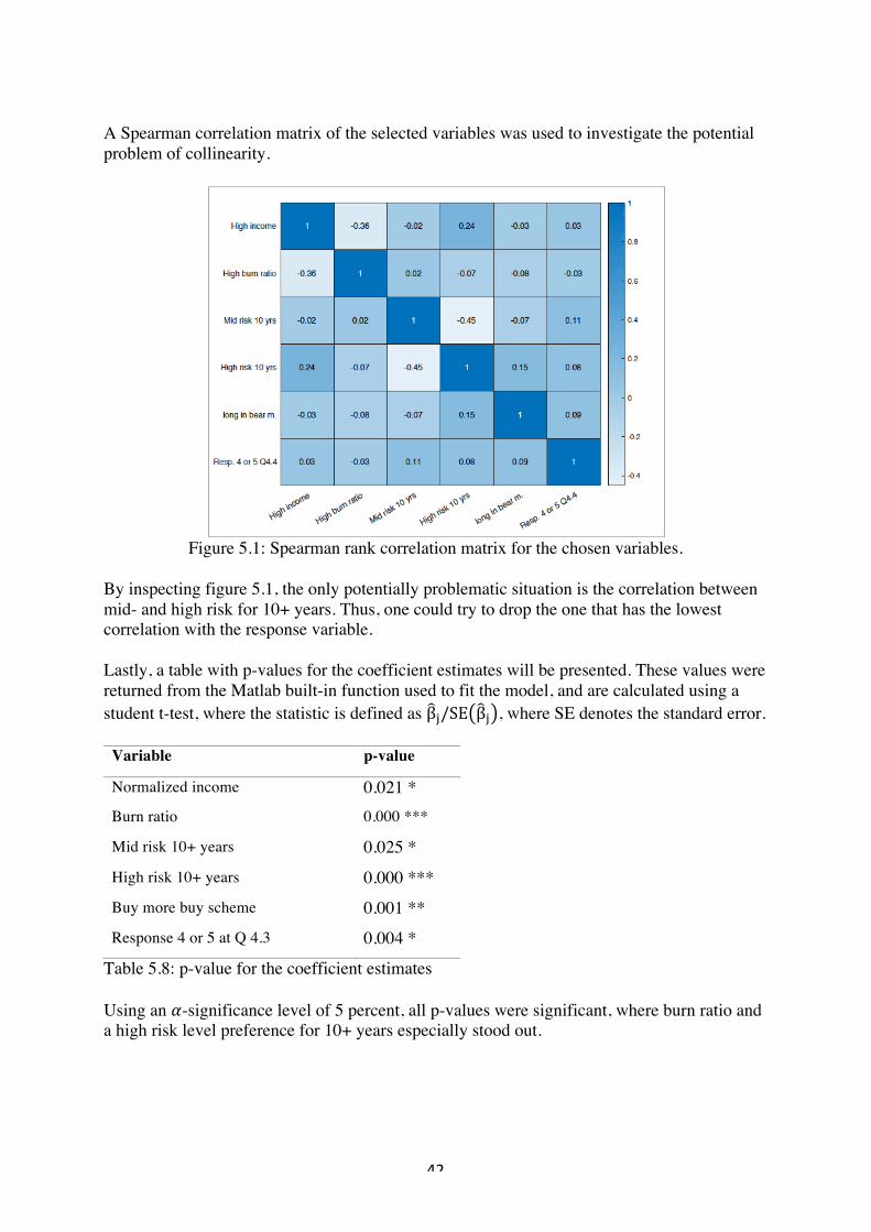
! 42!

!

A Spearman correlation matrix of the selected variables was used to investigate the potential problem of collinearity.

Figure 5.1: Spearman rank correlation matrix for the chosen variables.

By inspecting figure 5.1, the only potentially problematic situation is the correlation between mid- and high risk for 10+ years. Thus, one could try to drop the one that has the lowest correlation with the response variable. Lastly, a table with p-values for the coefficient estimates will be presented. These values were returned from the Matlab built-in function used to fit the model, and are calculated using a student t-test, where the statistic is defined as β±/SE β± , where SE denotes the standard error.

Variable p-value

Normalized income 0.021 * Burn ratio 0.000 ***

Mid risk 10+ years 0.025 *

High risk 10+ years 0.000 *** Buy more buy scheme 0.001 **

Response 4 or 5 at Q 4.3 0.004 *

Table 5.8: p-value for the coefficient estimates Using an Ç-significance level of 5 percent, all p-values were significant, where burn ratio and a high risk level preference for 10+ years especially stood out.

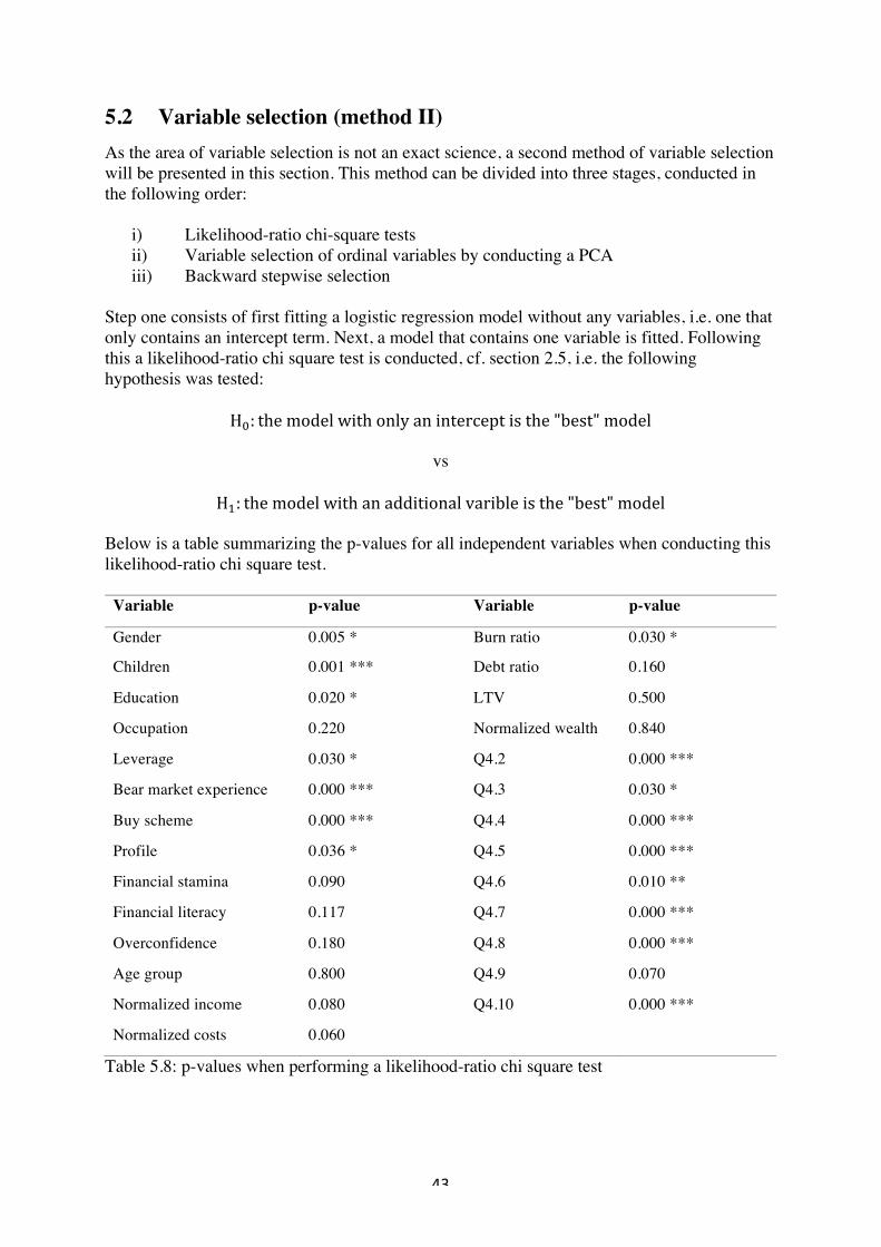
! 43!

!

5.2 Variable selection (method II) As the area of variable selection is not an exact science, a second method of variable selection will be presented in this section. This method can be divided into three stages, conducted in the following order:

i)! Likelihood-ratio chi-square tests ii)! Variable selection of ordinal variables by conducting a PCA iii)! Backward stepwise selection

Step one consists of first fitting a logistic regression model without any variables, i.e. one that only contains an intercept term. Next, a model that contains one variable is fitted. Following this a likelihood-ratio chi square test is conducted, cf. section 2.5, i.e. the following hypothesis was tested:

Ho: the&model&with&only&an&intercept&is&the&"best"&model

vs

HD: the&model&with&an&additional&varible&is&the&"best"&model Below is a table summarizing the p-values for all independent variables when conducting this likelihood-ratio chi square test.

Variable p-value Variable p-value

Gender 0.005 * Burn ratio 0.030 *

Children 0.001 *** Debt ratio 0.160

Education 0.020 * LTV 0.500

Occupation 0.220 Normalized wealth 0.840

Leverage 0.030 * Q4.2 0.000 ***

Bear market experience 0.000 *** Q4.3 0.030 *

Buy scheme 0.000 *** Q4.4 0.000 ***

Profile 0.036 * Q4.5 0.000 ***

Financial stamina 0.090 Q4.6 0.010 **

Financial literacy 0.117 Q4.7 0.000 ***

Overconfidence 0.180 Q4.8 0.000 ***

Age group 0.800 Q4.9 0.070

Normalized income 0.080 Q4.10 0.000 ***

Normalized costs 0.060

Table 5.8: p-values when performing a likelihood-ratio chi square test

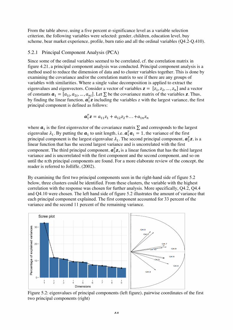
! 44!

!

From the table above, using a five percent Ç-significance level as a variable selection criterion, the following variables were selected: gender, children, education level, buy scheme, bear market experience, profile, burn ratio and all the ordinal variables (Q4.2-Q.410). 5.2.1 Principal Component Analysis (PCA) Since some of the ordinal variables seemed to be correlated, cf. the correlation matrix in figure 4.21, a principal component analysis was conducted. Principal component analysis is a method used to reduce the dimension of data and to cluster variables together. This is done by examining the covariance and/or the correlation matrix to see if there are any groups of variables with similarities. Where a single value decomposition is applied to extract the eigenvalues and eigenvectors. Consider a vector of variables ÷ = & ◊D, ◊E, … , ◊G and a vector of constants ÿD = ™DW, ™EW, … , ™GW . Let ∑ be the covariance matrix of the variables ÷. Thus, by finding the linear function, ÿD⁄÷ including the variables z with the largest variance, the first principal component is defined as follows:

ÿD⁄÷ = ™DD◊D + ™DE◊E+. . . +™DG◊G where ÿD is the first eigenvector of the covariance matrix ∑ and corresponds to the largest eigenvalue ÑD. By putting the ÿD to unit length, i.e.&ÿD⁄ÿD = 1, the variance of the first principal component is the largest eigenvalue ÑD. The second principal component, ÿE⁄÷, is a linear function that has the second largest variance and is uncorrelated with the first component. The third principal component, ÿº⁄÷, is a linear function that has the third largest variance and is uncorrelated with the first component and the second component, and so on until the n:th principal components are found. For a more elaborate review of the concept, the reader is referred to Jolliffe, (2002). By examining the first two principal components seen in the right-hand side of figure 5.2 below, three clusters could be identified. From these clusters, the variable with the highest correlation with the response was chosen for further analysis. More specifically, Q4.2, Q4.4 and Q4.10 were chosen. The left hand side of figure 5.2 illustrates the amount of variance that each principal component explained. The first component accounted for 33 percent of the variance and the second 11 percent of the remaining variance.

Figure 5.2: eigenvalues of principal components (left figure), pairwise coordinates of the first two principal components (right)

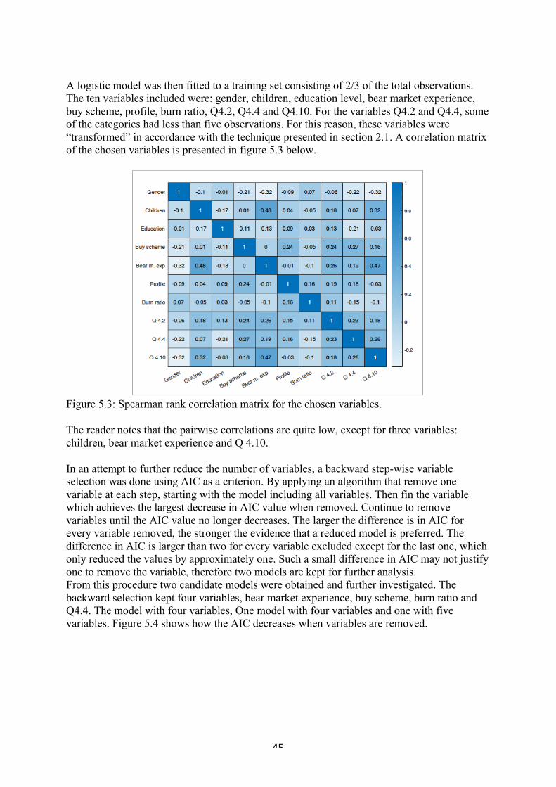
! 45!

!

A logistic model was then fitted to a training set consisting of 2/3 of the total observations. The ten variables included were: gender, children, education level, bear market experience, buy scheme, profile, burn ratio, Q4.2, Q4.4 and Q4.10. For the variables Q4.2 and Q4.4, some of the categories had less than five observations. For this reason, these variables were “transformed” in accordance with the technique presented in section 2.1. A correlation matrix of the chosen variables is presented in figure 5.3 below.

Figure 5.3: Spearman rank correlation matrix for the chosen variables. The reader notes that the pairwise correlations are quite low, except for three variables: children, bear market experience and Q 4.10. In an attempt to further reduce the number of variables, a backward step-wise variable selection was done using AIC as a criterion. By applying an algorithm that remove one variable at each step, starting with the model including all variables. Then fin the variable which achieves the largest decrease in AIC value when removed. Continue to remove variables until the AIC value no longer decreases. The larger the difference is in AIC for every variable removed, the stronger the evidence that a reduced model is preferred. The difference in AIC is larger than two for every variable excluded except for the last one, which only reduced the values by approximately one. Such a small difference in AIC may not justify one to remove the variable, therefore two models are kept for further analysis. From this procedure two candidate models were obtained and further investigated. The backward selection kept four variables, bear market experience, buy scheme, burn ratio and Q4.4. The model with four variables, One model with four variables and one with five variables. Figure 5.4 shows how the AIC decreases when variables are removed.

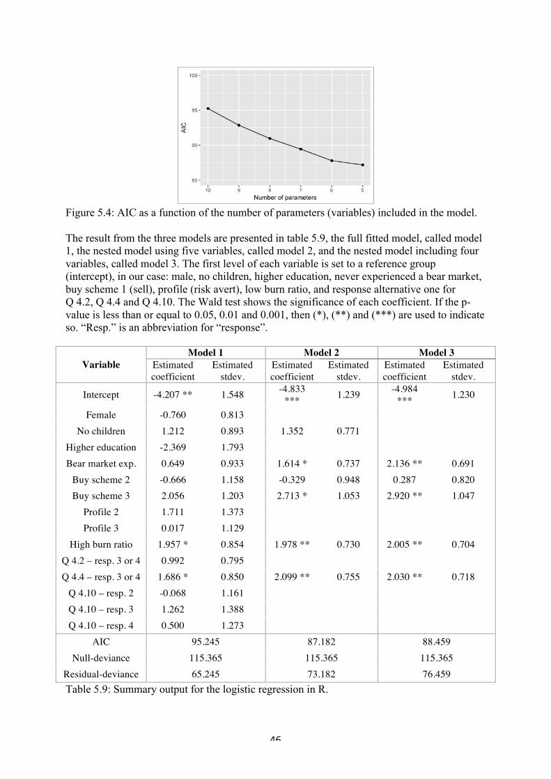
! 46!

!

Figure 5.4: AIC as a function of the number of parameters (variables) included in the model. The result from the three models are presented in table 5.9, the full fitted model, called model 1, the nested model using five variables, called model 2, and the nested model including four variables, called model 3. The first level of each variable is set to a reference group (intercept), in our case: male, no children, higher education, never experienced a bear market, buy scheme 1 (sell), profile (risk avert), low burn ratio, and response alternative one for Q 4.2, Q 4.4 and Q 4.10. The Wald test shows the significance of each coefficient. If the p-value is less than or equal to 0.05, 0.01 and 0.001, then (*), (**) and (***) are used to indicate so. “Resp.” is an abbreviation for “response”.

Variable Model 1 Model 2 Model 3

Estimated coefficient

Estimated stdev.

Estimated coefficient

Estimated stdev.

Estimated coefficient

Estimated stdev.

Intercept -4.207 ** 1.548 -4.833 *** 1.239 -4.984

*** 1.230

Female -0.760 0.813 No children 1.212 0.893 1.352 0.771

Higher education -2.369 1.793 Bear market exp. 0.649 0.933 1.614 * 0.737 2.136 ** 0.691

Buy scheme 2 -0.666 1.158 -0.329 0.948 0.287 0.820 Buy scheme 3 2.056 1.203 2.713 * 1.053 2.920 ** 1.047

Profile 2 1.711 1.373 Profile 3 0.017 1.129

High burn ratio 1.957 * 0.854 1.978 ** 0.730 2.005 ** 0.704 Q 4.2 – resp. 3 or 4 0.992 0.795 Q 4.4 – resp. 3 or 4 1.686 * 0.850 2.099 ** 0.755 2.030 ** 0.718

Q 4.10 – resp. 2 -0.068 1.161 Q 4.10 – resp. 3 1.262 1.388 Q 4.10 – resp. 4 0.500 1.273

AIC 95.245 87.182 88.459 Null-deviance 115.365 115.365 115.365

Residual-deviance 65.245 73.182 76.459 Table 5.9: Summary output for the logistic regression in R.

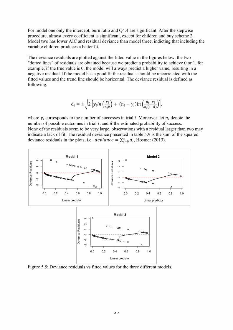
! 47!

!

For model one only the intercept, burn ratio and Q4.4 are significant. After the stepwise procedure, almost every coefficient is significant, except for children and buy scheme 2. Model two has lower AIC and residual deviance than model three, indicting that including the variable children produces a better fit. The deviance residuals are plotted against the fitted value in the figures below, the two "dotted lines" of residuals are obtained because we predict a probability to achieve 0 or 1, for example, if the true value is 0, the model will always predict a higher value, resulting in a negative residual. If the model has a good fit the residuals should be uncorrelated with the fitted values and the trend line should be horizontal. The deviance residual is defined as following:

d¤ = ± 2 HWõ[yzGz‹

+& [W − HW õ[GzfyzGz Df‹

,

where HW corresponds to the number of successes in trial >. Moreover, let [W denote the number of possible outcomes in trial >, and x the estimated probability of success. None of the residuals seem to be very large, observations with a residual larger than two may indicate a lack of fit. The residual deviance presented in table 5.9 is the sum of the squared deviance residuals in the plots, i.e. &V¶M>™[K¶ = VWG

WZo , Hosmer (2013).

Figure 5.5: Deviance residuals vs fitted values for the three different models.

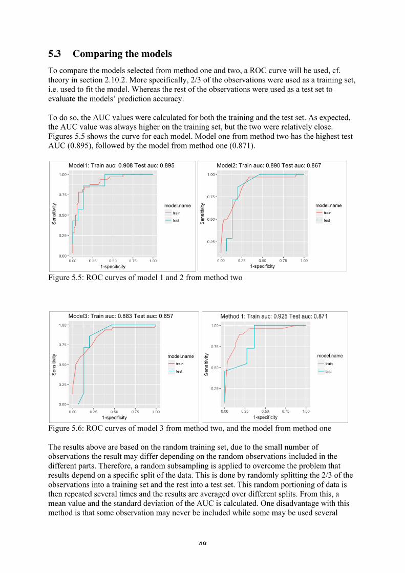
! 48!

!

5.3 Comparing the models To compare the models selected from method one and two, a ROC curve will be used, cf. theory in section 2.10.2. More specifically, 2/3 of the observations were used as a training set, i.e. used to fit the model. Whereas the rest of the observations were used as a test set to evaluate the models’ prediction accuracy. To do so, the AUC values were calculated for both the training and the test set. As expected, the AUC value was always higher on the training set, but the two were relatively close. Figures 5.5 shows the curve for each model. Model one from method two has the highest test AUC (0.895), followed by the model from method one (0.871).

Figure 5.5: ROC curves of model 1 and 2 from method two

Figure 5.6: ROC curves of model 3 from method two, and the model from method one The results above are based on the random training set, due to the small number of observations the result may differ depending on the random observations included in the different parts. Therefore, a random subsampling is applied to overcome the problem that results depend on a specific split of the data. This is done by randomly splitting the 2/3 of the observations into a training set and the rest into a test set. This random portioning of data is then repeated several times and the results are averaged over different splits. From this, a mean value and the standard deviation of the AUC is calculated. One disadvantage with this method is that some observation may never be included while some may be used several

! 49!

!

times, as opposed to the K-fold method which includes every observation. The results are presented in the table 5.10.

Model1 Model2 Model3 Method I Training

Mean AUC 0.924 0.887 0.874 0.954 Standard deviation 0.014 0.026 0.018 0.017

Test Mean AUC 0.845 0.830 0.850 0.907

Standard deviation 0.0403 0.085 0.083 0.056 Table 5.10: Results repeated random sub-sampling with 100 iterations. The repeated procedure shows that the model developed from method 1 has the highest mean value of both test and training AUC. This implies that this model is the best in discriminating between high- and low risk tolerance individuals.

! 50!

!

6 Analysis and conclusion In this section we will analyse and discuss the main findings made in this study. But before proceeding, some limitations of the study will be pointed out. To start off, the sample size is relatively small, with 110 unique observations. Accordingly, in order to make a robust analysis, the reader should consider that the results might have differed if more data was available. Also, worth mentioning is the risk of an non representative data sample. For example, the study was spread among friends and family members to the authors. Out of the 110 individuals, 24 were students and more than half of the participants consisted of 18-25 year olds. Moreover, 100 individuals had a university education, 65 % percent of the participants were male, and the economic situation seemed on average to be better than what is to be expected. Likewise, the majority of the answering individuals are living in, or nearby the area of Stockholm. Thus, one can conclude that the sample seems to be an un-representative mirror of the whole population. However, the main emphasis from the client’s perspective was primary to develop a methodology to classify the risk tolerance level of a retail investor, and to identify important factors. Furthermore, several psychometric questions were asked in the survey. The intention of doing so was to capture the risk aversion of an investor. Nonetheless, several of these questions exhibited a moderate to high correlation with each other, and could therefore be considered redundant. By using factor analysis, we were able to pin point three central questions that the client could use if the investor has a short attention span. Moreover, to ensure validity and reliability, the psychometric questions were borrowed from an industry leader known as FinaMetrica. In other words, it seems reasonable to assume that these questions, from a psychometric point of view, had been both been validated and pass all reliability criteria. However, it needs to be stressed that some of the questions, Q 4.8 and Q 4.1, could lay in the grey zone when it comes to fulfilling regulatory demands from the Swedish regulatory body, FI. Since these questions to different extents make the investor choose what risk they emphasize. Therefore, the client should probably consult with FI before using these questions. To re-connect to the findings in Agarwal (2017), among four factors, knowledge and age were considered paramount to explaining an investor’s goals. Further, the goals of an investor were at a five percent significance level, found to be dependent on both professional level (top, senior, middle, executive) and family situation. While occupation (type of employment) and income level were found to be independent of one’s goals. To compare these findings to ours, a two sample t-test and an F-test with a five percent Ç-significance level, likewise found that age, financial literacy and family situation (had children) played an important part in the investment process, but instead in terms of risk tolerance. To the contrary, we found that occupation and income level had a significant impact on one’s risk tolerance. The reason to conflicting findings, might partly be because of the underlying measurement: his intention was to map out factors related to investment goals, while ours was to find ones related to risk tolerance. Moreover, his participants had a different nationality (Indian), i.e. cultural differences might also influence, and his sample wasn’t as skewed in terms of both age and educational level. Additionally, Klement, J. (2015) had hypothesized little explanatory power of factors related to risk capacity, while our procedure found such factors to be of importance: both methods of variable selection found burn ratio to be of importance, and the first method found income to have significance. In a similar vein we also found that an investor’s prior experiences and socioeconomic factors possessed explanatory power. Besides this, Klement stated that 20-40

! 51!

!

percent of the variation of an investor’s asset allocation can be explained by genetics. Assuming there is a high to perfect correlation between an individual’s asset allocation and their risk tolerance, a good model could be assumed to be able to explain around 60-80 percent of the variance. Using the measure of úE, a number that by definition takes a value between zero and one, and is used to indicate the fraction of variance explained by a multiple regression model, one can investigate the potency of our explanans. Thus, by running a multiple regression using the selected variables in section 5.1 as covariates, and the test score as the response, one gets an úE value of 0.56. Indicating that a relatively large portion of the variance is accounted for, assuming that genetics is able to explain one to two fifths of the variance. However, the Pearson correlation coefficient between a participant’s test score and their asset allocation had a range of −0.28, 14 . Thus, a more thorough investigation ought to be done before making any hasty conclusions. To summarize, by applying logistic regression and factor analysis, our study was able to point towards significant factors contributing to classifying an individual as either risk averse or a risk lover. The three candidate models were comprised of features from both risk capacity, risk aversion, prior experiences, demographics and other socioeconomic factors. More specifically, a high burn ratio and a tactic of conducting a buy scheme in a bear market, were both included in all three models. As mentioned, a small subset of all psychometric variables turned out to be needed in the final model. Moreover, five to six variables seem sufficient enough to achieve a good model, evaluated by either the test AUC or the estimated accuracy ratio. Nonetheless, the small and potentially non representative sample size should be taken into consideration, that is, there are some inherent uncertainty left.

! 52!

!

7 Discussion and recommendation In this section, a brief discussion will follow with an emphasis on future research. Focusing on areas that might be appealing to the client. To start, of paramount interest ought to be to assure validity. To do so, a simple method could be to trace the behaviour of a customer, especially after a market correction. It would probably not be impermissible to assume that some investors during an extensive bull market develops an over confidence bias. Making commitments to a portfolio strategy that turned out a bit too excessive in relation to their actual risk tolerance. In other words, conducting surveys after greater market corrections, and calculating the correlation between responses prior to the correction, and the ones afterward, could be one way to assure validity of the risk profile. Furthermore, using a time series model to mimic the phenomenon of conditional heteroskedasticity associated with volatility in a customer’s portfolio, to relate to repeated measures of an investor’s risk tolerance, might also be of interest. To enhance predictability, one could allow for non-linear relationships among the covariates. That is, one could also investigate interaction effects among the variables. When doing so, one should according to James et al (2013) adhere to the hierarchical principle. I.e. one should make sure that all the lower effect involved in the interaction, are kept and not excluded. Simply put, if you have a two-way interaction you have to include both main effects. When touching on the subject of non-linearity, the predictability of other models, such as a regression trees and linear- or quadratic discriminant analysis, could also be investigated. In the initial stage of this thesis, the latter model was under consideration, but was discarded due the normality assumption about underlying distribution of the independent variables. Also, the client’s in-house expertise of logistic regression was another aspect that ruled out this alternative. Finally, some other miscellaneous thoughts will quickly be mentioned. When a greater data sample is available, the method of k-fold cross validation is from a computational perspective preferred. Also, another metric to ensure the quality of the models' prediction accuracy is Cohens Kappa, which is an accuracy measure that compensate for successes happening by chance. A working paper by Scholz and Tertilt (2017) that mentioned a method to “mine” for additional covariates could potentially be interesting for the client to re-view. Moreover, by using some readily available open source, one realises that there seems to be plenty of more sophisticated methods of the experimental kind, that could be used to create a more “nuanced” covariance matrix, cf. Chavent et al (2017) and Mori (2016), for an “introduction” to mixed data and nonlinear principal component analysis. Lastly, but of great importance, when conducting our brief literature study, the field of psychometrics is an own paradigm in its own right. While this thesis has just scratched upon its surface, there were some points that did stand out: the validity of a survey is assumed to depend on the number items included, and their reliability. Thus, it is all about validity and reliability.

! 53!

!

8 Bibliography In this section the references used in this thesis will be cited. 8.1 Literature Agarwal, S. (2017). Portfolio Selection Using Multi-Objective Optimisation. Cham, Switzerland: Springer Nature Agresti, A. (2002). Categorical Data Analysis. USA: John Wiley & Sons, Inc. Chavent, M., Simonet-Kuentz, V., Labenne, A. & Jérôme, S. (2017). Multivariate Analysis of Mixed Data: The R Package PCAmixdata. Available from: https://arxiv.org/pdf/1411.4911.pdf . Grable, E., J. (2017), 'Financial Risk Tolerance: a Psychometric Review ', CFA Institute Research Foundation. Available from: https://www.cfapubs.org/doi/pdf/10.2470/rfbr.v4.n1.1 [11 February 2018]. Jolliffe, T., I. (2002). Principal Component Analysis, 2nd Edition. New York, USA: Springer-Verlag. Klement, J. (2015), ‘Investor Risk Profiling: An Overview’, CFA Institute Research Foundation. Available from: https://www.cfapubs.org/doi/pdf/10.2470/rfbr.v1.n1.1 [10 February 2018] Graham, B. (2006). The Intelligent Investor – Revised Edition. New York, USA: HarperCollins Hosmer, W., D., Lemeshow, S. & Sturdivant, X., R. (2013). Applied Logistic Regression 3rd Edition. New Jersey, USA: John Wiley & Sons, Inc. James, G., Witten, D., Hastie, T. & Tibshirani. R. (2013). An Introduction to Statistical Learning: with Applications in R. New York, USA: Springer Johnson, A., Richard & Dean, W. & Wichern (1998). Applied Multivariate Statistical Analysis. New Jersey, USA: Springer Mori, Y., Kuroda, M. & Makino N. (2016). Nonlinear Principal Component Analysis and Its Applications. Singapore, Republic of Singapore: Springer Nature Olsson, Ulf (2002). Generalized Linear Models – An Applied Approach. Lund, Sweden: Studentlitteratur Ruey S. Tsay, (2010). Financial Times Series. New Jersey, USA: John Wiley & Sons Snedecor, G. W. & Cochran, W. G. (1980). Statistical Methods, 7th ed. Iowa State University Press, Ames, IA

! 54!

!

Scholz, P. & Tertilt, M. To Advise, or Not to Advise — How Robo-Advisors Evaluate the Risk Preferences of Private Investors. SSRN Working Paper. Last revised: 13 Jun 2017 8.2 Websites Statistik om Stockholm (2015), Stockholms stad, viewed 1 May 2018, < http://statistik.stockholm.se/publikationer/statistisk-arsbok-foer-stockholm/arsbokstabell-publ/arsbokstabeller-inkomster-skatter-och-priser-3 > PM Finansinspektionen (2016), Automatiserad rådgivning, viewed 29 May 2018, <https://www.fi.se/contentassets/1adb77c775d54fe4b612f89971faeb7f/autoradgivning_2016-12-30.pdf> Hushållens boendeutgift (2015), SCB, viewed 1 May 2018, <http://www.statistikdatabasen.scb.se/pxweb/sv/ssd/START__HE__HE0202/HE0202T01/?rxid=6480c240-e5d8-4d70-bb37-dd2cbb42ae77 >

9. Appendix In this section the questionnaire in its full entity will be presented. N.B. that due to the targeted audience, the survey was in its original shape presented in Swedish. A1 – Demographics In this subsection, questions related to risk capacity and demographics will be presented. Risk capacity is defined as one’s ability to bear financial risk, cf. [reference to some paper]. It is assumed that this trait is partly time-dependent and static. To get a general picture of the participants’ ability to bear financial risks, the following questions were asked: 1.1!Gender: man or woman

1.2!Age 1.3!Do you have children under the age of 19?

If true: !! How many? !! Do you have sole custody?

1.4!What is your educational background?

!! High school !! Vocational university !! University

! 55!

!

1.5!What is your primary source of revenue?

!! Full time employee !! Self-employed !! Student !! Job seeker !! Retired !! Other

1.6!What is your average monthly income? 1.7!What is your average monthly cost?

1.8!What is a rough estimate of the value of your assets?

!! Private savings (e.g. stocks, funds, commodities) !! Buffer savings (e.g. money market account) !! Real estate (you share) !! Other

1.9!What is the estimated value of your debt?

!! Property loans !! Unsecured debt !! Student loan !! Other

A2 – Prior experience & attitude to risk In this subsection, questions aimed at extracting the participants’ prior experience with financial risk taking, investments and financial risk preferences will be presented. 2.1 What are your primary sources of guidance or “tools” when making a financial decision? Rank the following alternatives (1-5), one being the most important source.

!! Financial advisor !! Own research !! Blogs and/or podcasts !! Family / friends !! Other

! 56!

!

2.2 Have you ever owned financial assets during a financial crisis, or during a major bear market? If true: 2.2.1! How was your long term savings affected?

!! Decreased my monthly savings !! Unchanged !! Increased my monthly savings

If false: 2.2.2 Imagine you’d have a monthly savings scheme concentrated to equity index funds. Over the last six months, the leading equity index in has dropped significantly and your portfolio is down 30 percentage points on a year to day basis. How do you expect this to affect your monthly savings?

!! I would decrease my monthly savings !! Let it remain the same !! I would increase it

2.3 Have you ever borrowed money to make an investment (other than for your home)?

!! Yes !! No

2.4 For the following three investment horizons, what is your preferred level of risk?

!! 0-2 years: low, mid, high !! 3-10 years: low, mid, high !! 10+ years: low, mid, high

2.5 Remind yourself of a situation where a financial decision has gone noticeably wrong. How hard of a time was it for you to mentally to recover from this event?

!! Very hard !! Somewhat hard !! Somewhat easy !! Very easy

A3 – Financial literacy In this subsection questions aimed at portraying the financial literacy level of the participants will be presented. The questions were taken, and in some instances re-phrased, from the well-known test called “the big five - financial literacy test”. Moreover, the correct answers will be highlighted. 3.1 Suppose you have $100 in a savings account earning 2 percent interest a year. After five years, how much would you have?

!! More than $110 (correct) !! Exactly $110 !! Less than $110 !! Do not know

! 57!

!

3.2 Imagine that the interest rate on your savings account is 3.5 percent a year and inflation is 5 percent a year. After one year, would the money in your account:

!! Buy you more than it does today !! Buy exactly the same !! Buy you less than today (correct) !! Do not know

3.3 Is it true that: buying a single company's stock usually provides a safer return than a stock mutual fund.

!! True !! False (correct) !! Do not know

3.4 Is it true that: a 15-year mortgage typically requires higher monthly payments than a 30-year mortgage, but the total interest over the life of the loan will be less.

!! True (correct) !! False !! Do not known

3.5 If interest rates fall, what will typically happen to bond prices? They will typically:

!! Rise (correct) !! Fall !! Do not know

The reasoning behind the last question is that when interest rates fall, bond prices rise. This is because as interest rates fall, newer bonds that come to the market pays a lower yield than older bonds, all else being equal, making older bonds more attractive and worth more. 3.6 How many correct answers do you expect to get?

!! 0!!! 1!!! 2!!! 3!!! 4!!! 5!

! 58!

!

A4 – Psychometric part The questions depicted in this subsection were aimed at revealing a retail investor’s “true” risk profile. That is, the aim was to extract data that could be combined in some appropriate manner to generate a measureable variable, giving some indication of an investor’s inclines and likelihood towards taking financial risks. As the author(s) had no prior experience of ‘risk-profiling’, a sample of appropriate questions were taken from the Australian based company, FinaMetrica, specialising in financial risk profiling. 4.1!Compared to others, how do you rate your willingness to take financial risks?

(1)!Extremely low (2)!Low (3)!High (4)!Extremely high

4.2 When you think of the word "risk" in a financial context, which of the following words comes to mind first?

(1)!Danger (2)!Uncertainty (3)!Opportunity (4)!Thrill

Q4.3 Have you ever invested a large sum in a risky investment mainly for the "thrill" of seeing whether it went up or down in value?

(1)!Never (2)!Yes, very rarely (3)!Yes, somewhat rarely (4)!Yes, somewhat frequently (5)!Yes, very frequently.

Q4.4 How would your best friend describe you as a risk taker?

(1)!A gambler (2)!Takes financial risks after performed research (3)!Reluctant (4)!Tends to avoid taking risks

Q4.5 When faced with a major financial decision, are you more concerned about the possible losses or the possible gains?

(1)!Always the possible losses (2)!Usually the possible losses (3)!Usually the possible gains (4)!Always the possible gains

! 59!

!

Q4.6 Imagine you were in a job where you could choose whether to be paid salary, commission or a mix of both. Which would you pick?

(1)!All salary (2)!Mainly salary (3)!Equal mix of salary and commission (4)!Mainly commission (5)!All commission

Q4.7 If you were given the following investment opportunities, which one would you choose?

(1)!Earn 2000 SEK (2)!Earn 8000 SEK, risk 2000 SEK (3)!Earn 26 000 SEK, risk 8 000 SEK (4)!Earn 48 000, risk 24 000 SEK

Q4.8 If you had to invest 200 000 SEK, which one of the following asset allocation schemes would you subscribe to?

(1)!60% in low risk assets, 30% in mid risk assets, 10% in high risk assets (2)!30% in low risk assets, 40% in mid risk assets, 30% in high risk assets (3)!10% in low risk assets, 40% in mid risk assets, 50% in high risk assets

Q4.9 Five years ago you bought stocks in a company, believing it had great upside potential. However, due to bad management decisions the stock price plummeted, consequently you sold and experienced a painful loss. Now, the company has a new management team and experts find it likely that the company will generated above average returns. Given your prior experience, would you buy stocks in the company?

(1)!Definitely not (2)!Probably not (3)!Unsure / do not know (4)!Probably (5)!Definitely

Q4.10 You are participating in a televised game show, and are able to pick one of the following four alternatives, which one would you pick?

(1)! With certainty win 10 000 SEK (2)!A 50 % probability to win 50 000 SEK (3)!A 25 % probability to win 100 000 SEK (4)!A 5 % probability to win 1 000 000 SEK

TRITA -SCI-GRU 2018:253

www.kth.se