Financial Market Dislocations - World...
53
Financial Market Dislocations Paolo Pasquariello 1 February 15, 2012 1 c ° 2012 Paolo Pasquariello, Department of Finance, Ross School of Business, University of Michigan, [email protected]. I am grateful to CIBER and the Q Group for financial support. I benefited from the comments of Rui Albuquerque, Torben Andersen, Andrew Ang, Ravi Bansal, Sreedhar Bharath, Robert Dittmar, Wayne Ferson, Mark Huson, Ming Huang, Charles Jones, Andrew Karolyi, Ralph Koijen, Francis Longstaff, Darius Miller, Lubos Pastor, Amiyatosh Purnanandam, Angelo Ranaldo, Gideon Saar, Jules van Binsbergen, Frank Warnock, and seminar participants at the 2011 NBER SI Asset Pricing meetings, the 2011 FRA conference, University of Michigan, Michigan State University, and Cornell University. Any remaining errors are my own.
Transcript of Financial Market Dislocations - World...

Financial Market Dislocations
Paolo Pasquariello1
February 15, 2012
1 c° 2012 Paolo Pasquariello, Department of Finance, Ross School of Business, University of Michigan,[email protected]. I am grateful to CIBER and the Q Group for financial support. I benefited fromthe comments of Rui Albuquerque, Torben Andersen, Andrew Ang, Ravi Bansal, Sreedhar Bharath,Robert Dittmar, Wayne Ferson, Mark Huson, Ming Huang, Charles Jones, Andrew Karolyi, RalphKoijen, Francis Longstaff, Darius Miller, Lubos Pastor, Amiyatosh Purnanandam, Angelo Ranaldo,Gideon Saar, Jules van Binsbergen, Frank Warnock, and seminar participants at the 2011 NBER SIAsset Pricing meetings, the 2011 FRA conference, University of Michigan, Michigan State University,and Cornell University. Any remaining errors are my own.

Abstract
Dislocations occur when financial markets, operating under stressful conditions, experience large,
widespread asset mispricings. This study documents systematic financial market dislocations in
world capital markets and the importance of their fluctuations for expected asset returns. Our
novel, model-free measure of these dislocations is a monthly average of six hundred abnormal
absolute violations of three textbook arbitrage parities in stock, foreign exchange, and money
markets. We find that investors demand economically and statistically significant risk premiums
to hold financial assets performing poorly during market dislocations.
JEL classification: G01; G12
Keywords: Asset Pricing; Dislocations; Expected Returns; Financial Crisis; Arbitrage

1 Introduction
Financial market dislocations are circumstances in which financial markets, operating under
stressful conditions, cease to price assets correctly on an absolute and relative basis. The goal
of this empirical study is to document the aggregate, time-varying extent of financial market
dislocations in world capital markets and to investigate whether their fluctuations affect expected
asset returns.
The investigation of financial market dislocations is of pressing interest. When “massive” and
“persistent,” these dislocations pose “a major puzzle to classical asset pricing theory” (Fleck-
enstein et al., 2010). The turmoil in both U.S. and world capital markets in proximity of the
2008 financial crisis is commonly referred to as a major “dislocation” (e.g., Matvos and Seru,
2011). Policy makers have recently begun to treat such dislocations as an important, yet not
fully-understood source of financial fragility and economic instability when considering macro-
prudential regulation (Kashyap et al., 2010; Hubrich and Tetlow, 2011). Lastly, the recurrence of
severe financial market dislocations over the last three decades (e.g., Mexico in 1994-1995; East
Asia in 1997; LTCM and Russia in 1998; Argentina in 2001-2002) has prompted institutional
investors to revisit their decision-making and risk-management practices.
Financial market dislocations are elusive to define, and difficult to measure. The assessment of
absolute mispricings is subject to considerable debate and significant conceptual and empirical
challenges (O’Hara, 2008). The assessment of relative mispricings stemming from arbitrage
breakdowns is less controversial. According to the law of one price – a foundation of modern
finance – arbitrage activity should ensure that prices of identical assets converge, lest unlimited
risk-free profits may arise. Extant research reports frequent deviations in several no-arbitrage
parities in the foreign exchange, stock, bond, and derivative markets, both during normal times
and in correspondence with known financial crises; less often these observed deviations provide
1

actionable arbitrage opportunities.1 An extensive literature attributes these deviations to explicit
and implicit “limits” to arbitrage activity.2
In this paper, we propose and construct a model-free measure of financial market dislocations
based on innovations in daily observed violations of six hundred permutations of three textbook
no-arbitrage conditions. The first one, known as the Covered Interest Rate Parity (CIRP), is a
relationship between spot and forward exchange rates and the two corresponding nominal interest
rates ensuring that riskless borrowing in one currency and lending in another in international
money markets while hedging currency risk generates no riskless profit (e.g., Bekaert and Hodrick,
2009). The second one, known as the Triangular Arbitrage Parity (TAP), is a relationship
between exchange rates ensuring that cross-rates (e.g., yen per British pounds) are aligned with
exchange rates quoted relative to a “vehicle currency” (e.g., the dollar or the euro; Kozhan and
Tham, 2010). The third one, known as the American Depositary Receipt Parity (ADRP), is a
relationship between exchange rates, local stock prices, and U.S. stock prices ensuring that the
prices of cross-listed and home-market shares of stocks are aligned (e.g., Gagnon and Karolyi,
2010). Focus on these parities allows us to document systematic market dislocations in multiple
stock, foreign exchange, and money markets spanning nearly four decades (1973-2009).
Our aggregate measure of monthly financial market dislocations is a cross-permutation, equal-
weighted average of abnormal individual deviations from their no-arbitrage parities. Each parity’s
individual arbitrage deviation is computed as the standardized absolute log difference between
1A comprehensive survey of this vast literature is beyond the scope of this paper. Recent studies find violationsof the triangular arbitrage parity (Marshall et al., 2008; Kozhan and Tham, 2010), covered interest rate parity(Akram et al., 2008; Coffey et al., 2009; Griffoli and Ranaldo, 2011), cross-listed stock pairs parity (Pasquariello,2008; Gagnon and Karolyi, 2010), Siamese twins parity (Mitchell et al., 2002), TIPS-Treasury arbitrage parity(Campbell et al., 2009; Fleckenstein et al., 2010), off-the-run Treasury bond-note parity (Musto et al., 2011), CDS-bond yield parity (Duffie, 2010; Garleanu and Pedersen, 2011), convertible bond parity (Mitchell and Pulvino,2010), futures-cash parity (Roll et al., 2007), and put-call parity (Lamont and Thaler, 2003; Ofek et al., 2004).
2Arbitrage activity may be impeded by such financial frictions as transaction costs, taxes, holding costs, short-sale and other investment restrictions (surveyed in Gagnon and Karolyi, 2010), information problems (Grossmanand Miller, 1988), agency problems (De Long et al., 1990; Shleifer and Vishny, 1997), risk factors (e.g., Pontiff,1996a, b), execution risk (Stein, 2009; Kozhan and Tham, 2010), noise trader risk (e.g., Shleifer, 2000), supplyfactors (Fleckenstein et al., 2010), fire sales (Kashyap et al., 2010; Shleifer and Vishny, 2011), competition (Kondor,2009), margin constraints (Garleanu and Pedersen, 2011), funding liquidity constraints and slow-moving capital(e.g., Brunnermeier and Pedersen, 2009; Duffie, 2010; Gromb and Vayanos, 2010).
2
actual and theoretical prices. Absolute arbitrage violations are common, positively correlated,
and often economically large over our sample period.3 At each point in time, individual deviations
are standardized using exclusively their current and past realizations. This procedure ensures
comparability of innovations in absolute deviations across different parities without introducing
a look-ahead bias in the measure. The resulting market dislocation index (MDI) is higher in
correspondence with greater-than-normal marketwide arbitrage parity violations. The index
is easy to calculate, and displays sensible properties as a gauge of aggregate financial market
dislocations. It exhibits cycle-like dynamics – e.g., rising and falling in proximity of well-known
episodes of financial turmoil in the 1970s, 1980s, and 1990s – and reaches its height during
the most recent financial crisis. It is higher during U.S. recessions, in the presence of greater
fundamental uncertainty, lower systematic liquidity, and greater financial instability, but also
in less turbulent times. Yet, a wide array of state variables can only explain up to 53% of its
dynamics. These properties suggest MDI to be a good candidate proxy for the many frictions
and barriers affecting financial markets’ ability to correctly price traded assets.
Accordingly, it seems natural to conjecture the risk of financial market dislocations to be
important for asset pricing. As observed by Fleckenstein et al. (2010), sizeable and time-varying
no-arbitrage violations indicate the presence of forces driving asset prices that are absent in
standard, frictionless asset pricing models. A copious literature relates several frictions to (and
biases in) investors’ trading activity to asset prices.4 The direct measurement of these forces
is however notoriously difficult. Studying the extent of arbitrage breakdowns across assets and
markets may help us establish their empirical relevance for asset returns. As such, financial
market dislocations may be a priced state variable. Investors may require a compensation (in
3For instance, absolute log deviations average 21 basis points (bps) for CIRP, 0.05 bps for TAP, and 219 bpsfor ADRP.
4See, e.g., Amihud and Mendelson (1986), Constantinides (1986), Brennan and Subrahmanyam (1996), Bren-nan et al. (1998), Vayanos (1998), Shleifer (2000), Amihud (2002), Huang (2003), Pastor and Stambaugh (2003),Acharya and Pedersen (2005), Duffie et al. (2005, 2007), Baker and Wurgler (2006), and Sadka and Scherbina(2007).
3

the form of higher expected returns) for holding assets with greater sensitivity to dislocation risk.
We investigate this possibility within both the U.S. and a sample of developed and emerging
stocks and foreign exchange. Our evidence indicates that these assets’ sensitivities to MDI
have significant effects on the cross-section and time-series properties of their returns. We find
that stock and currency portfolios with higher negative “financial market dislocation betas” –
i.e., experiencing lower realized returns when MDI is higher – exhibit higher expected returns.
For example, between 1973 and 2009, the estimated market dislocation risk premium for U.S.
stock portfolios formed on size and book-to-market sorts is roughly −3% per annum, even after
controlling for their sensitivities to the market. Similarly, the market price of MDI risk for
portfolios of currencies sorted by their interest rates is −2.4% per annum when assessed over
the available sample period 1983-2009. The estimated MDI risk premium for country stock
portfolios is smaller, ranging between −0.7% and −0.1% (when net of the world market factor).
These estimates are both statistically and economically significant, for they imply non-trivial
compensation per average MDI beta: E.g., as high as 8.5% per annum for U.S. stock portfolios,
6.7% for international stock portfolios, and 7.0% for a zero-cost carry trade portfolio (long high-
interest rate currencies and short low-interest rate currencies). Furthermore, the MDI betas
explain up to 37% (17%) of the cross-sectional variation in expected U.S. (international) excess
stock returns, and up to 71% of the cross-sectional variation in excess currency returns.
Intuitively, this evidence suggests that investors require a positive premium to hold asset
portfolios performing poorly during financial market dislocations (i.e., with negative MDI be-
tas), but are willing to pay a negative premium to hold portfolios providing insurance against
that risk (i.e., with positive MDI betas). Consistently, when sorting U.S. stocks into portfolios
according to their historical MDI betas, we find that stocks with higher ex ante negative sen-
sitivity to market dislocation risk tend to exhibit both higher expected returns and positive ex
post such sensitivity. In particular, a spread between the bottom and top deciles of historical
MDI beta stocks earns annualized abnormal returns (“alphas”) of 7.2% – after accounting for
4

sensitivities to the market, size, value, and momentum factors – while displaying a positive
overall-period MDI beta. Thus, stocks doing poorly during prior financial market dislocations
(i.e., with negative historical MDI betas when MDI realizations are positive) may subsequently
do poorly during more normal times (i.e., with positive post-ranking MDI betas when MDI re-
alizations are small or negative). Investors demand sizeable compensation to hold these stocks,
especially in the recent, more turbulent sub-period 1994-2009: GMM-estimated market disloca-
tion risk premium after controlling for the aforementioned four traded factors is roughly 2.74%
per annum, implying a statistically and economically significant compensation for the spread’s
post-ranking MDI beta of 10.6%. Lastly, in the time-series, MDI has some predictive power for
future asset returns over both short and longer horizons. For instance, a one standard deviation
positive shock to MDI predicts (an average of) 0.9% lower excess returns next month but 1.1%
higher six-month-ahead cumulative excess returns (consistent with our cross-sectional results)
for several developed and emerging stock portfolios between 1994 and 2009.
Numerous empirical studies document the relation between individual frictions absent from
classical finance theory (e.g., liquidity, information, sentiment, noise, financial distress) and ex-
pected asset returns, hedge fund returns, or asset pricing anomalies (e.g., Pastor and Stambaugh,
2003; Baker and Wurgler, 2006; Sadka and Scherbina, 2007; Avramov et al., 2010; Fleckenstein
et al., 2010; Hu et al., 2010; Alti and Tetlock, 2011; Stambaugh et al., 2011).5 Others emphasize
the potential importance of rare events and crises for the cross-section of asset returns (e.g.,
Veronesi, 2004; Barro, 2006; 2009; Gabaix, 2007; Bianchi, 2010; Bollerslev and Todorov, 2011).
To our knowledge, our model-free analysis of systematic financial market dislocation risk – one
encompassing both observable and unobservable sources of mispricings – and its role in asset
5For instance, Hu et al. (2010) show that a measure of “noise” constructed as the difference between actualand interpolated Treasury bond yields spikes during episodes of marketwide illiquidity (see also Musto et al., 2011)and is related to cross-sectional returns of hedge funds and currency carry trades. The literature proposes severalalternative yield curve interpolation models, but finds all of them to be plagued by errors both in normal timesand during periods of financial turmoil (e.g., Gürkaynak et al., 2007). This raises the question of whether yielddifferentials from these models are akin to mispricings and can be conceptually attributed to liquidity effects.
5

pricing is novel to the literature.
We proceed as follows. In Section 2, we construct our measure of financial market dislocations
and describe its empirical properties. In Section 3, we present and discuss the results of a wide
array of asset pricing tests. We conclude in Section 4.
2 The financial market dislocation index
Financial market dislocations entail large, widespread mispricings of traded financial securities.
Motivated by their frequent occurrence, over the last few decades financial economics has ad-
vocated the important role of frictions and biases for the process of price formation in capital
markets. As previously mentioned, it has proposed and tested several explanations for why mis-
pricings may arise, persist, and wane. Measuring the direct extent of these frictions and biases
– and their relevance for asset pricing – is challenging, and often practical only “in the context
of a series of ‘special cases”’ (Gagnon and Karolyi, 2010, p. 54).
In this study, we circumvent this issue by constructing a composite index of price disloca-
tions in global stock, foreign exchange, and money markets. The index captures the systematic
component of six hundred potential violations of three textbook no-arbitrage parities in those
markets. Hence, it measures the systematic significance of observable and unobservable factors
behind their occurrence. Next, we describe each of these parities, the procedure for the construc-
tion of our index, and the index’s basic properties. In Section 3, we then investigate whether
financial market dislocation risk – i.e., the risk that frictions and biases in capital markets may
lead to mispricings – is priced in U.S. and international stock returns.
2.1 Arbitrage parities
We estimate the observed magnitude of mispricings in global capital markets by measuring vio-
lations of the Covered Interest Rate Parity, the Triangular Arbitrage Parity, and the American
6

Depositary Receipt Parity. There are several advantages to focusing on these parities. Assessing
their violations does not require us to take a stance on any asset pricing model. Their violations
imply impediments to the enforcement of the law of one price via arbitrage within some of the
largest, most liquid financial markets in the world. The literature surveyed in the Introduction
attributes these violations to such explicit and implicit barriers to arbitrage as taxes, (inventory)
holding costs, transaction costs, short-sale restrictions, opportunity cost of capital, idiosyncratic
risk, liquidity risk, slow moving capital, funding liquidity, market freezes, rollover risk, (counter-
party) default risk, execution risk, exchange controls, information problems, agency problems, or
political risk. Data availability allows us to assess the systematic, time-varying extent of these
(often difficult-to-measure) impediments over a sample period spanning almost four decades.
2.1.1 Covered interest rate parity
The first set of arbitrage deviations in our study stems from violations of the Covered Interest
Rate Parity (CIRP). According to the CIRP, in absence of arbitrage, borrowing in any currencyA
for T−t days (at interest cost rA,t,T ), exchanging the borrowed amount to currency B at the spot
exchange rate St,A/B, lending in currency B (at interest rB,t,T ), and hedging the foreign exchange
risk of repaying the original loan plus interest at the forward exchange rate Ft,T,A/B generates no
profits. The absence of covered interest rate arbitrage in international money markets implies
the following theoretical (∗), no-arbitrage forward exchange rate between any two currencies A
and B:
F ∗t,T,A/B = St,A/B
µ1 + rA,t,T1 + rB,t,T
¶, (1)
where St,T,A/B (Ft,T,A/B) is the spot (forward) exchange rate on day t expressed as units of
currency A for one unit of currency B.
While conceptually simple, the actual implementation of non-convergence CIRP arbitrage if
7

the CIRP in Eq. (1) is violated (Ft,T,A/B 6= F ∗t,T,A/B) is more involved. E.g., if Ft,T,EUR/USD <
F ∗t,T,EUR/USD, one would profit by buying USD for EUR in the forward market at a low price and
then selling USD for EUR at a high synthetic forward price using the spot and money markets
(i.e., borrowing the initial amount of EUR, converting them into USD, and lending USD). This
strategy requires accounting for synchronous prices and rates, transaction costs, and borrowing
and lending on either secured terms (at “repo” and “reverse repo” rates) or unsecured terms (at
overnight bid and offer rates, with accompanying index swaps).6 Both funding and trading costs
and explicit and implicit limits to arbitrage typically create no-arbitrage bands around theoretical
CIRP levels. Both have been shown to vary during “tranquil versus turbulent periods” (e.g.,
Frenkel and Levich, 1975, 1977; Coffey et al., 2009; Griffoli and Ranaldo, 2011). Data and
structural limitations (e.g., non-binding pricing) make measurement of actual CIRP arbitrage
profits challenging and feasible only over a few, most recent years (e.g., see Akram et al., 2008;
Fong et al., 2010; Griffoli and Ranaldo, 2011).
We intend to capture the systematic component of CIRP violation levels and dynamics across
the broadest spectrum of currencies and maturities over the longest feasible sample period. To
that purpose (as in the literature), our sample is made of daily indicative spot and forward
prices (as observed at 4 p.m. Greenwich Mean Time [GMT]) of nine exchange rates among five
of the most liquid (and relatively free-floating) currencies in the global foreign exchange market
(CHF/USD, GBP/USD, EUR/USD, JPY/USD, CHF/EUR, GBP/EUR, JPY/EUR, CHF/GBP,
JPY/GBP), and the corresponding LIBOR rates at seven maturities (7, 30, 60, 90, 180, 270,
and 360 days), void of transaction costs, between May 1, 1990 and December 31, 2009.7 This
dataset comes from Thomson Reuters Datastream (Datastream).8 For each of the resulting 63
6See Griffoli and Ranaldo (2011) for further details and evidence of actual CIRP profits during the 2008financial crisis.
7CHF is the Swiss Franc; EUR is the European Euro; GBP is the British Pound; JPY is the Japanese Yen;USD is the U.S. Dollar. LIBOR rates are computed by the British Bankers Association (BBA) as arithmeticaverages of contributor banks’ interbank offers at around 11 a.m. GMT.
8Exchange and money market rates for EUR/USD, GBP/EUR, CHF/EUR, and JPY/EUR are available inDatastream from the date the euro is officially introduced (January 1, 1999); prior forward and LIBOR data for
8

CIRP permutations (i), we compute daily (t) absolute log differences (in basis points [bps], i.e.,
multiplied by 10, 000) between actual and CIRP-implied forward exchange rates: CIRPi,t =¯̄̄ln¡Ft,T,A/B
¢− ln
³F ∗t,T,A/B
´¯̄̄× 10, 000.9
Panel A of Table 1 reports summary statistics for CIRPm, the monthly average of daily mean
observed CIRP violations CIRPi,t across all available currency-maturity permutations. We plot
its time-series in Figure 1a. During most circumstances, CIRP violations are low. Systematic
absolute percentage deviations of market forward exchange rates from their theoretical levels
average 21 bps (i.e., 0.21%), fluctuate between 10 and 15 bps during the late 1990s, and are as
low as 9 bps by the end of 2006. Yet, CIRP violations also display meaningful intertemporal
dynamics. Over our sample period, CIRPm trends first upward, then downward. It also often
spikes in proximity of well-known episodes of financial turmoil. Most notably (and consistent with
recent aforementioned studies), average CIRP deviations reach a maximum (84 bps) in October
2008 (immediately following the Lehman bankruptcy) and remain higher than the historical
averages for many months afterwards.
2.1.2 Triangular arbitrage parity
The second set of arbitrage deviations in our study stems from violations of the Triangular Arbi-
trage Parity (TAP). Triangular arbitrage is a sequence of contemporaneous transactions keeping
cross-rates – exchange rates not involving vehicle currencies (USD or EUR), e.g., JPY/GBP –
in line with exchange rates quoted versus vehicle currencies (e.g., JPY/USD and USD/GBP).
According to the TAP, in absence of arbitrage the spot cross-rate between any two currencies A
and B should satisfy the following relation with the spot exchange rates of each with a third,
such European currencies as DEM, FRF, and ITL is not. For simplicity and uniformity across exchange rates(e.g., when considering national holidays, special circumstances for fixing and value dates, as well as evolvingday-count conventions [and their possibly conflicting interpretations] over the sample period), interest rates arecompounded using a 30/360 convention. The effect of employing “market” day-count conventions, when feasible,on our analysis is immaterial.
9We filter the Datastream dataset for potential data errors and exclude daily CIRP deviations of 10% or more,i.e., when CIRPi,t ≥ 1, 000 bps. The evidence that follows is unaffected by our filtering procedure.
9

vehicle currency (V ):
S∗t,A/B = St,A/V × St,V/B. (2)
When Eq. (2) is violated (St,A/B 6= S∗t,A/B), implementation of the triangular arbitrage is
straightforward for it involves simultaneously selling and buying three exchange rates in the spot
market. E.g., if St,CAD/GBP < S∗t,CAD/GBP and V = USD, one would simultaneously buy GBP
for CAD, sell the ensuing units of GBP for USD, and sell those USD for CAD; this strategy
would be profitable for it implies buying GBP at a low CAD price and selling GBP at a high
CAD price (Bekaert and Hodrick, 2009). This trading strategy does not rely on convergence to
parity and is typically unimpeded by taxes, short-selling, or other regulatory constraints. Similar
data limitations as for the CIRP prevent the large-scale measurement of actual TAP arbitrage
profits. Rather, we focus on extracting the systematic component of daily TAP violations for the
most cross-rates (with respect to either USD or EUR [DEM before January 1, 1999]) among the
most liquid, relatively free-floating currencies over the longest feasible sample period, between
January 1, 1973 and December 31, 2009: AUD, CAD, CHF, FRF, GBP, ITL, JPY.10 These
daily indicative spot exchange rates (as observed at 3 p.m. Eastern Standard Time [EST]) come
from the Pacific Exchange Rate Service database (Pacific). For each of the resulting 122 TAP
permutations (i), we compute daily (t) absolute log differences (in bps) between actual and
TAP-implied spot cross rates: TAPi,t =¯̄̄ln¡St,A/B
¢− ln
³S∗t,A/B
´¯̄̄× 10, 000.11
Transaction costs are minimal in the highly liquid spot foreign exchange market (BIS, 2010).
Not surprisingly, the literature finds that TAP violations are small, yet persistent (e.g., Aiba
10AUD is the Australian Dollar; CAD is the Canadian Dollar; DEM is the German Mark; FRF is the FrenchFranc; ITL is the Italian Lira.11We filter the Pacific dataset for errors (and unreasonably large TAP deviations) using the same procedure
employed for the Datastream sample and CIRP deviations (see Section 2.1.1). We also verify that observed TAPviolations in our dataset are not due to rounding of prices from Eq. (2) and/or from direct-to-indirect quoteconversion (i.e., from St,A/B =
¡St,B/A
¢−1). We accommodate any deviation from the latter in the dataset by
considering TAP violations of either S∗t,A/B or S∗t,B/A separately.
10

et al., 2002; Marshall et al., 2008; Kozhan and Tham, 2010). Consistently, Panel A of Table
1 reports that mean monthly absolute percentage TAP deviations across all available cross-
rate permutations, TAPm, average 0.05 bps (i.e., 0.0005%). TAPm’s plot (in Figure 1b) however
shows TAP violations to ebb and flow in long cycles, especially during the 1970s and 1980s, before
suddenly increasing in the late 1990s (around the launch of the euro), reaching a maximum of
0.0009% in January 2005, and staying relatively high afterwards. Interestingly, these dynamics
appear to be only weakly related to those of average cross-currency CIRP violations (e.g., a
correlation of −0.160 with CIRPm in Table 1). Thus, TAP violations may provide distinct
information on the extent and time-series of financial market dislocations (and the frictions
driving them) over our sample period.
2.1.3 ADR parity
The last set of arbitrage deviations in our study stems from violations of the American De-
positary Receipt Parity (ADRP). Companies can list shares of their stock for trading in several
markets (especially in the U.S.) besides their domestic ones in several forms, from global regis-
tered offerings to direct listings (e.g., Karolyi, 2006). Of these cross-listing mechanisms, American
Depositary Receipts (ADRs) are the most common. ADRs are dollar-denominated, negotiable
certificates, traded on U.S. stock markets, representing a pre-specified amount (“ratio”) of a for-
eign company’s publicly traded equity held on deposit at a U.S. depositary bank.12 Depositary
banks (e.g., Bank of New York, JPMorgan Chase) charge small custodial fees for converting all
stock-related payments in USD and, more generally, facilitating ADRs’ convertibility into the
underlying foreign market shares and vice versa. The holder of an ADR can redeem that certifi-
cate into the underlying shares from the depositary bank at any time for a fee; conversely, new
12A minority of companies, mostly Canadian, cross-list their stock in the U.S. in the form of ordinary shares.Ordinary shares are identical certificates trading in both the U.S. and, e.g., Canada (i.e., with a ratio of one; seeBekaert and Hodrick, 2009). In the U.S., “Canadian ordinaries” trade like U.S. firms’ stock, require no depositarybank, but are subject to specific clearing and transfer arrangements. The literature typically groups ordinariestogether with ADRs (e.g., Gagnon and Karolyi, 2010).
11

ADRs can be created at any time by depositing the ratio of foreign shares at the depositary bank.
If ADRs and the underlying equity are perfect substitutes, absence of arbitrage implies that the
unit price of an ADR, Pi,t, should at any time be equal to the dollar price of the corresponding
amount (qi) of home-market shares, as follows:
P ∗i,t = St,USD/H × qi × PHi,t , (3)
where PHi,t is the unit stock price of the underlying foreign shares in their local currency H.
Implementation of a literal ADR arbitrage when Eq. (3) is violated (Pi,t 6= P ∗i,t) is complex.
E.g., if Pi,t < P ∗i,t one would simultaneously buy the ADR, retrieve the underlying home-market
shares from the depositary bank (a process known as “cancellation”), sell those shares in their
home market, and convert the foreign currency sale proceeds to USD. Alternatively, simpler
convergence-based trading strategies would involve, e.g., buying the “cheap” asset (in this case
the ADR at Pi,t) and selling the “expensive” one (in this case the underlying foreign shares at PHi,t).
Several studies (exhaustively surveyed in Karolyi, 2006) provide evidence of significant deviations
of observed ADR prices from their theoretical parities. Any of the many aforementioned frictions,
risks, and barriers to trading in the literature may impede the successful exploitation of both
types of ADR arbitrage. ADRs’ fungibility, as captured by Eq. (3), is also limited by such
additional factors as conversion fees, holding fees, custodian safekeeping fees, foreign exchange
transaction costs, service charges, transfer arrangements, or (one-way and two-way) cross-border
ownership restrictions (Gagnon and Karolyi, 2010).
As the above discussion makes clear, measuring ADR parity violations has the potential to
shed light on the extent and dynamics of a wide array of impediments to arbitrage in the U.S.
stock market, in international stock markets for the underlying stocks, and/or in the correspond-
ing foreign exchange markets. As for CIRP and TAP violations, data availability and structural
limitations (e.g., imperfect price synchronicity, stale pricing) preclude a comprehensive inves-
12

tigation of actual ADR arbitrage profits.13 Accordingly, in this study we aim to capture the
systematic component of ADR violations across the broadest spectrum of stocks (and curren-
cies) over the longest feasible sample period. To that purpose, we obtain the complete sample
of all foreign stocks cross-listed in the U.S. either as ADRs or as ordinary shares compiled by
Datastream at the end of December 2009. Consistent with the literature (e.g., Pasquariello,
2008; Gagnon and Karolyi, 2010), we exclude from this sample non-exchange-listed ADRs (Level
I, trading over-the-counter in the “pink sheet” market), SEC Regulation S shares, private place-
ment issues (Rule 144A ADRs), and preferred shares, as well as ADRs and foreign shares with
missing Datastream pair codes.14 Our final sample is made of 410 home-U.S. pairs of closing stock
prices (and ratios) for exchange-listed (on NYSE, AMEX, or NASDAQ; sponsored or unspon-
sored) Level II and Level III (capital raising) ADRs from 41 developed and emerging countries
between January 1, 1973 and December 31, 2009.15
For each of these pairs (i), we use Eq. (3) and exchange rates from Pacific to compute daily
(t) absolute log differences (in bps) between actual and theoretical ADR prices: ADRPi,t =¯̄ln (Pi,t)− ln
¡P ∗i,t¢¯̄× 10, 000. Panel A of Table 1 contains descriptive statistics for ADRPm,
the monthly average of daily mean ADRP violations among all available pairs in the sample.16
Average absolute deviations from ADR parity are large, about 219 bps (i.e., 2.19%), and subject
to large fluctuations.17 As displayed in Figure 1c, ADRPm is generally declining over our sample
13For instance, Gagnon and Karolyi (2010) address non-synchronicity between foreign stock and ADR pricesby employing available intraday price and quote data for the latter (from TAQ) at a time corresponding to theclosing time of the equity market for the underlying (if their trading hours are at least partially overlapping).However, the trading hours of Asian markets do not overlap with U.S. trading hours. In addition, TAQ data isavailable only from January 1, 1993.14We cross-check the accuracy of Datastream pairings by comparing them with those reported in the Bank of
New York Mellon Depositary Receipts Directory, available at http://www.adrbnymellon.com/dr_directory.jsp.15Sponsored ADRs are initiated by the foreign company of the underlying shares. Unsponsored ADRs are
initiated by a depositary bank. Most developed ADRs in our sample are from Canada (67), the Euro area (58),the United Kingdom (43), Australia (30), and Japan (24); emerging cross-listings include stocks traded in HongKong (54), Brazil (23), South Africa (14), and India (10), among others.16We further filter our dataset for errors by excluding daily absolute deviations for ADRs with share prices less
than $5 and greater than $1, 000, as well as daily ADRP deviations of 10% or more, i.e., when ADRPi,t ≥ 1, 000bps.17Summary statistics for ADRPm are similar to (albeit smaller than) those reported in Gagnon and Karolyi
(2010, Table 2) for signed log-price differences based on synchronous prices when possible.
13

period, hinting at a broad trend for lower barriers to (arbitrage) trading and greater world
financial market integration. Yet, in correspondence with episodes of financial turmoil, ADR
parity deviations tend to increase and become more volatile (e.g., in the 1970s, during the
Mexican Peso and Asian crises, or in 2008).18 Some of these dynamics appear to relate to those
of CIRP violations in Figure 1a (a correlation of 0.314 with CIRPm in Table 1), presumably
via mispricings in the foreign exchange market, but not to the time series of TAP violations in
Figure 1b (a correlation of −0.078 with TAPm).
2.2 Index construction
The three textbook no-arbitrage parities described in Sections 2.1.1 to 2.1.3 yield 595 daily
potential mispricings in the global stock, foreign exchange, and money markets. Each of them is
only an imprecise estimate of the extent of dislocations in the market(s) in which it is observed
(as well as of the explicit and implicit impediments behind its occurrence). However, Table
1 indicates that their realizations are only weakly correlated across parities. Figure 1 further
suggests that observed mispricings tend to persist over time, perhaps reflecting the permanent
nature of some impediments to arbitrage or data and structural limitations to their accurate
measurement. This discussion suggests that an average of all abnormal arbitrage parity violations
may measure systematic financial market dislocation risk more precisely.
We construct our novel index of dislocation risk in two steps. First, on any day t we stan-
dardize each parity’s individual arbitrage deviation (CIRPi,t, TAPi,t, ADRPi,t) relative to its
historical distribution on that day: CIRP zi,t, TAPzi,t, ADRP
zi,t.
19 This step allows to assess the
extent to which each realized individual absolute no-arbitrage violation was historically large on
the day it occurred without introducing look-ahead bias, while making these violations compa-
rable across and within different parities. Equivalently, each so-defined standardized arbitrage
18Consistently, Pasquariello (2008) finds evidence of greater ADRP violations for emerging markets stocksduring recent financial crises.19To that end, on any day t we exclude parity deviations with less than 22 past and current realizations.
14

breakdown represents an innovation with respect to its historical mean (i.e., expected) mispric-
ing. Their paritywide monthly means (CIRP zm, TAPzm, ADRP
zm, in Panel B of Table 1) are
frequently negative, often statistically significant, (less than perfectly) correlated, and subject
to large intertemporal fluctuations.20 Second, we compute a monthly index of financial market
dislocation risk, MDIm, as the equal-weighted, cross-parity average of these monthly means.
This step allows to isolate the common, systematic component of the cross-section of innovations
in (i.e., abnormal) absolute no-arbitrage parity violations in our sample at each point in time
parsimoniously, while preserving their time-series properties. By construction, the index (plotted
in Figure 2) is higher in correspondence with greater-than-normal marketwide mispricings, i.e.,
in the presence of historically large financial market dislocations.
2.3 Index properties
The composite indexMDIm, based on minimal manipulations of observed model-free mispricings
in numerous equity, foreign exchange, and money markets, is easy to calculate and displays
sensible properties as a measure of systematic financial market dislocation risk.
Estimated correlations in Panel B of Table 1 indicate thatMDIm loads positively on average
abnormal no-arbitrage violations in each of the three textbook parities (CIRP, TAP, and ADRP).
Saliently, its plot (in Figure 2) displays several short-lived upward and downward spikes, as well
as meaningful longer-lived, cycle-like dynamics over our sample period 1973-2009.21 Many of
20Monthly averaging smooths potentially spurious daily variability in these normalized arbitrage parity viola-tions, e.g., due to price staleness or non-synchronicity.21According to Cochrane (2001, p. 150), risk factors in linear asset pricing models “do not have to be totally
unpredictable,” as long as they are expressed in the “right units” since these models are often applied to excessreturns without identifying the conditional mean of the discount factor (as in Sections 3.1 and 3.2). The marketdislocation index MDIm is not highly persistent (e.g., a first-order autocorrelation of 0.70) and measures innova-tions in relative mispricings with respect to their historical levels. Further, the lack of strong predictive evidencein Section 3.3 suggests our cross-sectional inference is unlikely to be contaminated by correlation between MDImand future excess returns. Alternatively, the time-series of month-to-month changes in the index, ∆MDIm, mea-sures innovations in relative mispricings only with respect to their most recent levels. Hence, ∆MDIm may notcapture long-lasting dislocations, like those observed during the last quarter of 2008 in the aftermath of LehmanBrothers’ default. The correlation between MDIm and ∆MDIm is 0.39. The inference reported in the paper isrobust to using ∆MDIm instead of MDIm.
15

these spikes and cycles occur in proximity of well-known episodes of financial turmoil in the last
four decades: The Mideast oil embargo in the Fall of 1973, the oil crisis in the late 1970s, the
emerging debt crisis in 1982, the U.S. stock market crash in October 1987, the European currency
crisis in 1991-1992, the collapse of bond markets in 1994, the Mexican Peso crisis in 1994-1995,
the Asian crisis in 1997, the Russian default and LTCM debacle in the Fall of 1998, the internet
bubble during the late 1990s, 9/11, and the quant meltdown in August 2007. Consistent with
this chronology, most positive realizations of our index (i.e., most abnormal mispricings) occur in
the latter portion of our sample. The index is highest in October 2008, in the wake of Lehman’s
default and in the midst of the most significant economic crisis and financial freeze since the Great
Depression. It is plausible to conjecture that in those circumstances, impediments to trading and
arbitrage may have become more severe, and asset mispricings larger and more widespread.
Further insight on the nature and properties of our index of standardized innovations in
arbitrage parity violations comes from regressing its realizations on the change in several U.S.
and international, economic and financial market variables, in Table 2. Regressing MDIm on
similarly normalized levels of these variables yields nearly identical inference. Variable selection
is driven by the observation (motivated by the aforementioned literature on limits to arbitrage)
that mispricings are more likely during periods of U.S. and/or global economic and financial
uncertainty, illiquidity, and overall financial distress.22 Accordingly, we find MDIm to be higher
during U.S. recessions (in column (1) of Table 2), as well as in correspondence with higher world
stock market volatility (in columns (1) and (4)), lower U.S. systematic liquidity (as estimated by
22The monthly regressors in Table 2 include U.S. stock returns (from Kenneth French’s website), a dummyequal to one during official NBER recessions, Chauvet and Piger’s (2008) historical U.S. recession probabilities(from Piger’s website), VIX (average of daily VIX, from CBOE), world market returns (from MSCI) and returnvolatility (its annualized 36-month rolling standard deviation), U.S. risk-free rate (one-month Treasury bill rate,from Ibbotson Associates), Pastor and Stambaugh’s (2003) liquidity measure (from Pastor’s website), slope of U.S.yield curve (average of ten-year minus one-year constant-maturity Treasury yields, from the Board of Governors),U.S. bond yield volatility (annualized average of rolling standard deviation of five-year constant-maturity Treasuryyields, as in Hu et al., 2010), TED spread (average of three-month USD LIBOR minus constant maturity Treasuryyields, from Datastream), default spread (average of Aaa minus Baa corporate bond yields, from Moody’s), andfinancial stress index (STLFSI, from the Federal Reserve Bank of St. Louis, capturing the comovement of 18financial variables such as stock and bond returns and return volatility, various yield spreads, and TIPS break-eveninflation rates).
16

Pastor and Stambaugh, 2003; in columns (1) and (4)), and higher marketwide financial instability
(e.g., higher Federal Reserve of St. Louis’ financial stress index; in columns (3) and (4)), yet
also during more “tranquil” times (e.g., lower “TED” spread between LIBOR and Treasury
Bill rates; in columns (3) and (4)). Ceteris paribus, average abnormal arbitrage breakdowns
weakly increase in correspondence with greater marketwide “risk appetite” (lower CBOE VIX
index, in column (4); e.g., Bollerslev et al., 2009) or U.S. stock market downturns (and the
accompanying illiquidity, as argued by Chordia et al., 2001; in columns (1) and (4)), but are
insensitive to changes in the slope and volatility of U.S. interest rates (in column (2)), flight
to quality (e.g., lower U.S. risk-free rates, in column (2); see Hu et al., 2010), or default risk
(e.g., higher Moody’s Baa-Aaa corporate bond spread; in column (3)). In aggregate, all of these
proxies can only explain up to 53% of MDIm’s dynamics (in column (4)).23
These properties suggest our index of abnormal no-arbitrage violations to be a reasonable,
non-redundant proxy for financial markets’ ability to correctly price traded assets.
3 Is financial market dislocation risk priced?
Our measure of financial market dislocation risk, MDIm, is based on a large cross-section of no-
arbitrage parity violations in global stock, foreign exchange, and money markets over nearly four
decades. As discussed above,MDIm has several desirable properties. It is parsimonious and easy
to compute; it relies on model-free assessment of asset mispricings; it is privy of look-ahead bias;
and it displays sensible time-series features, consistent with commonly-held notions of market
dislocations. In this section we investigate whether so-defined financial market dislocation risk is
a priced state variable. We concentrate on equity and foreign exchange markets, because of the
potential sensitivity of stock and currency returns to systematic mispricings and the availability
23In unreported analysis excluding the most recent period of financial turmoil because of data availability, wealso findMDIm to weakly increase in correspondence with greater investor sentiment (as estimated in Baker andWurgler, 2006) or greater worldwide intensity of capital controls (as estimated in Edison and Warnock, 2003).
17

of established pricing benchmarks. We test whetherMDIm is related to the cross-section of U.S.
and international stock portfolio returns, the cross-section of U.S. stock returns, the cross-section
of currency portfolio returns, and future aggregate stock and currency portfolio returns.
3.1 Financial market dislocations and risk premiums: Stocks
3.1.1 Univariate MDI beta estimation
We begin by exploring the exposure of equity market portfolios to financial market dislocation
risk. Preliminarily, we follow the standard cross-sectional approach by proceeding in two steps
(e.g., Campbell et al., 1997). First, we run time-series regressions to estimate the sensitivity
of the monthly excess dollar return of each equity portfolio i, Ri,m, to our aggregate abnormal
mispricing index MDIm:
Ri,m = βi,0 + βi,MDIMDIm + εi,m. (4)
Second, we estimate the dislocation risk premium λMDI using all equity portfolios:
E (Ri,m) = λ0 + λMDIβi,MDI . (5)
We consider two samples of 26 U.S. and 50 international equity portfolios over the period
1973-2009. The U.S. sample includes the U.S. market (RM,m) and 25 U.S. portfolios formed on
size (market equity) and book-to-market (book equity to market equity), from French’s website.24
The international sample is unbalanced and includes the world market portfolio (RWM,m), 23
developed, and 26 emerging country portfolios (listed in Table 4), from MSCI.25 Tables 3 and
24See http://mba.tuck.dartmouth.edu/pages/faculty/ken.french/data_library.html. In unreported analysis, wefind similar inference from studying a larger sample of 100 portfolios sorted on size and book-to-market.25World and developed country portfolio returns are available from January 1973, with the exception of Finland
(January 1982), Greece, Ireland, New Zealand, and Portugal (January 1988). Emerging country returns areavailable from January 1988, with the exception of China, Colombia, India, Israel, Pakistan, Peru, Poland, SouthAfrica, and Sri Lanka (January 1993), Czech Republic, Egypt, Hungary, Morocco, and Russia (January 1995).
18

4 report estimated MDI betas from Eq. (4) for U.S. and international portfolios, respectively.
Figures 3a and 3b display scatter plots of their annualized mean percentage excess returns ver-
sus these MDI betas. The largest, circular scatters refer to the broad U.S. and world market
portfolios; scatters with dark (white) background refer to statistically (in)significant MDI betas,
at the 10% level or less. Estimated MDI betas in Tables 3 and 4 are large, mostly (and often
highly) statistically significant, and always negative: Excess returns of U.S. and international
stock portfolios tend to be lower in correspondence with abnormally high financial market dislo-
cations – i.e., when arbitrage breakdowns are (in aggregate) greater than their historical means
(MDIm > 0). MDI betas are more negative for “riskier” portfolios: Portfolios of smaller U.S.
stocks, U.S. stocks with higher book-to-market, and stocks of emerging countries.
Figures 3a and 3b suggest that stock portfolios with more negative MDI betas have higher
average excess returns. Accordingly, estimates of Eq. (5), in Panel A of Table 5, indicate that
the annualized price of financial market dislocation risk is negative (λMDI < 0) and statistically
significant within both U.S. and international stock portfolio samples.26 Dislocation risk premi-
ums are economically significant, amounting to 3% and 0.5% per unit of MDI beta – i.e., 8.5%
and 3.8% per average MDI beta – for U.S. and international stock portfolios, respectively. The
accompanying adjusted R2 (R2a) of 34% and 15% suggest that financial market dislocation risk
can explain a meaningful portion of the cross-section of equity portfolio returns. These properties
are generally robust across sample sub-periods, although absolute estimated λMDI and Eq. (5)’s
cross-sectional explanatory power are greater in the first sub-period (1973-1993) for U.S. portfo-
lios, and in the second sub-period (1994-2009) for country portfolios.27 Intuitively, this evidence
is consistent with the notion that investors find financial market dislocations undesirable. Thus,
26Annualized risk premium estimates are computed multiplying monthly estimates by 12. Because of MDIm’srelatively large variance (e.g., see Panel B of Table 1), similar inference is drawn from applying the errors-in-variables correction described in Shanken (1992) to their conventional t-statistics (in Tables 5 and 10). TheGMM-based procedure of Section 3.1.2 yields heteroskedasticity-robust inference as well (e.g., Cochrane, 2001).27Those uneven sub-periods are chosen to correspond to the even sub-periods (1978-1993, 1994-2009) stemming
from the analysis of the cross-section of U.S. stock returns in Section 3.2.
19

they require a compensation for holding stock portfolios with greater exposure to that risk, i.e.,
performing more poorly in circumstances when asset mispricings are abnormally large.
3.1.2 Multivariate MDI beta estimation
Financial market dislocation risk may be subsumed by additional systematic risk factors. For
instance, Figure 3 and Tables 3 and 4 show that both the U.S. and world market portfolios
are highly sensitive to MDIm. We investigate this possibility by employing the multivariate
asset pricing model in Pastor and Stambaugh (2003). This model allows to assess the marginal
contribution of MDIm to the cross-section of equity portfolio returns while accounting for their
sensitivities to other factors. Specifically, we define a multivariate extension of Eq. (4):
Rm = β0 +BFm + βMDIMDIm + εm, (6)
where Rm is a N × 1 vector of excess portfolio returns, Fm is a K × 1 vector of “traded” factors,
B is a N ×K matrix of factor loadings, and β0 and βMDI are N × 1 vectors. Assuming that the
N portfolios are priced by the factor betas in Eq. (6) implies that
E (Rm) = BλF + βMDIλMDI . (7)
Since our index MDIm is not the payoff of a trading strategy, in general λMDI 6= E (MDIm),
while λF = E (Fm) for traded factors Fm. Hence, substitution of Eq. (7) in Eq. (6), after taking
expectations of both its sides, yields the restriction:
β0 = βMDI [λMDI −E (MDIm)] . (8)
At this stage we assume that, besides MDIm, U.S. (world) stock market risk is the main
traded risk factor for U.S. (international) stock portfolios: Fm = RM,m (Fm = RWM,m) in Eq.
20

(6). The U.S. portfolios in our sample are already sorted on firm size and book-to-market.
The World CAPM is the most common international asset pricing model (Bekaert and Hodrick,
2009). In the next section we consider additional, popular traded factors when examining the
cross-section of individual U.S. stock returns. We then estimate the MDI risk premium separately
for the remaining 25 U.S. stock portfolios and the 49 country equity portfolios in our sample using
the GMM procedure described in Pastor and Stambaugh (2003).28 Panel B of Table 5 reports the
corresponding estimates of annualized λMDI , their asymptotic t-statistics, as well as asymptotic
chi-square J -tests for the over-identifying restriction in Eq. (8).29 Full-period and sub-period
GMM estimates of dislocation risk premiums for U.S. and eligible international stock portfolios
are always negative (albeit unsurprisingly smaller and less often statistically significant than in
Panel A of Table 5) even after accounting for the effect of market risk. For instance, MDI risk
premiums per average MDI beta range between 2.04% and 2.43% for U.S. portfolios, and between
0.62% and 1.76% for country portfolios.30
Overall, U.S. and international stock portfolios’ sensitivities to financial market dislocations
appear to explain a non-trivial portion of these portfolios’ risk, one that is not captured by
market fluctuations and for which investors require meaningful compensation.
3.1.3 Portfolio construction by financial market dislocation betas
The evidence in Tables 3 to 5 provides support to the notion that financial market dislocation
risk is priced in the cross-section of U.S. and international stock portfolio returns. In this section
28To that purpose, let γ be the set of 2 + N (K + 1) unknown parameters: λMDI , βMDI , B, andE (MDIm). Next, define fm (γ) =
¡hm⊗εm
MDIm−E(MDIm)
¢, where h0m = (1 F 0m MDIm) and εm = Rm −
βMDI [λMDI −E (MDIm)] − BFm − βMDIMDIm. Then, bγGMM = argmin g (γ)0Wg (γ), where g (γ) =
(1/M)PMm=1 fm (bγ) fm (bγ)0 and bγ = argmin g (γ)0 g (γ).
29In all cases, this restriction cannot be rejected at any conventional significance level. Notably, because of dataavailability, Eqs. (6) to (8) can be jointly estimated via GMM only for 18 developed country portfolios (excludingFinland, Greece, Ireland, New Zealand, and Portugal) over 1973-2009 and 1973-1993, and for 44 country portfolios(excluding Czech Republic, Egypt, Hungary, Morocco, and Russia) over 1994-2009.30Amending Eq. (4) to include (world) market returns and estimating Eq. (5) after accounting for (world)
market risk premiums in mean excess U.S. (country) portfolio returns yields similar inference.
21

we investigate further whether the cross-section of U.S. stocks’ expected returns is related to
those stocks’ sensitivities to abnormal marketwide mispricings, i.e., to their MDI betas. We
follow a portfolio-based approach similar to the one in Pastor and Stambaugh (2003). At the
end of every year of our sample, starting with 1977, we sort all stocks into ten portfolios based on
stocks’ estimated MDI betas over the previous five years. We then regress the ensuing stacked,
post-formation returns on standard asset pricing factors. According to the literature, estimated
nonzero intercepts (alphas) would suggest that MDI betas explain a component of expected stock
returns not captured by standard factor loadings.
Our dataset comes from the monthly tape of the Center for Research in Security Prices
(CRSP). It comprises monthly stock returns and values for all domestic ordinary common stocks
(CRSP share codes 10 and 11) traded on the NYSE, AMEX, and NASDAQ between January
1, 1973 and December 31, 2009.31 At the end of each year (e.g., on month m), for each stock j
with 60 months of available data through m we estimate its MDI beta as the slope coefficient
βj,MDI on MDIm in the following multiple regression of its monthly excess return Rj,m:
Rj,m = βj,0 + βj,MRM,m + βj,SSMBm + βj,BHMLm + βj,MDIMDIm + ηj,m, (9)
where SMBm and HMLm are the popular size-based and book-to-market-based traded factors
of Fama and French (1993), from French’s website. We then sort all stocks by their pre-ranking,
historical MDI betas βj,MDI into ten portfolios (from the lowest, 1, to the highest, 10), and
compute their value-weighted returns for the next twelve months.32 Equally-weighted portfolios
yield virtually identical inference. Repeating this procedure over our sample and stacking decile
31As customary, this restriction excludes Real Estate Investment Trusts (REITs), closed-end funds, Shares ofBeneficial Interest (SBIs), certificates, units, Americus Trust Components, companies incorporated outside theU.S., and American Depositary Receipts (ADRs). The latter is important since ADR mispricings contribute toour financial market dislocation index. When forming MDI beta-sorted portfolios, we also exclude stocks withprices either below $5 or above $1, 000.32On average, each portfolio contains 124 stocks. No portfolio contains less (more) than 71 (181) stocks.
Notably, on each portfolio formation month, this procedure sorts stocks using exclusively information availableup to that month.
22

returns across years generates ten monthly return series from January 1978 to December 2009.33
Panel A of Table 6 reports post-ranking MDI betas from running Eq. (9) for each historical
MDI beta-decile portfolio i, as well as for the 1-10 spread portfolio going long stocks with the
lowest (i.e., most negative) pre-ranking MDI betas (decile 1) and short stocks with the highest
(i.e., most positive) pre-ranking MDI betas (decile 10). Focus on this spread portfolio is mo-
tivated by the evidence in the previous section that stock portfolios with the greatest negative
exposure to financial market dislocation risk experience the highest mean excess returns. Panel
B of Table 6 reports additional features of these portfolios: Their average market capitalization
and sensitivities to the broad market, size, and book-to-market factors, as well as to the traded
momentum factor (MOMm, also from French’s website). Lower (i.e., often more negative) his-
torical MDI beta stocks are generally larger; their portfolios weakly tilt toward growth stocks
(negative HML betas) and past losers (negative MOM betas). Interestingly, post-ranking MDI
betas tend to decline across deciles, and the spread portfolio’s MDI beta is 2.72, with a t-statistic
of 2.64. Ceteris paribus, stocks doing relatively poorly during past financial market dislocations
(negative MDI betas when MDIm > 0) may subsequently do relatively poorly during normal
times (positive post-ranking MDI betas when MDIm ≤ 0).34 However, stocks doing relatively
well during past financial market dislocations (positive MDI betas when MDIm > 0) tend to
be insensitive to innovations in relative mispricings afterwards (small, insignificant post-ranking
MDI betas). In light ofMDIm’s cycle-like dynamics over our sample period (see Figure 3), these
properties suggest stocks in lower (i.e., more negative) pre-ranking MDI beta decile portfolios to
be riskier than their high decile counterparts.
33Alternatively, we sort stocks by predicted MDI betas from a linear model including such stock characteristicsas their cross-sectionally demeaned historical MDI betas, past six-month cumulative returns and return standarddeviation, natural log of lagged stock price and number of shares outstanding. Historical MDI beta, price,and return volatility are the most significant predictors over our sample period; yet, sign and magnitude of allpredictor coefficients display non-trivial intertemporal dynamics. The inference based on portfolios sorted onthese predicted betas is qualitatively comparable to the one based on historical MDI betas.34Equivalently, these same stocks, having performed relatively well during past normal times (negative MDI
betas when MDIm ≤ 0), may continue to do so during subsequent financial market dislocations (positive post-ranking MDI betas when MDIm > 0).
23

Our analysis reveals that investors demand sizeable compensation to hold those riskier stocks.
Table 7 reports post-ranking annualized alphas for each pre-ranking MDI beta portfolio and
the 1-10 spread with respect to three traded factor specifications: CAPM (the market factor:
RM,m), Fama-French (the market, size, and book-to-market factors: RM,m, SMBm, HMLm),
and Fama-French plus Momentum (RM,m, SMBm, HMLm, MOMm). All three spread portfolio
alphas are positive, large, and statistically significant both over the full sample (1978-2009) and
in the later sub-period (1994-2009), i.e., especially when abnormal mispricings appear to occur
most frequently (i.e., when positive realizations of MDIm occur most often, see Figure 2). For
instance, four-factor alpha for the 1-10 spread portfolio is 7.23% (t = 2.92) over 1978-2009, 1.90%
(t = 0.65) over 1978-1993 (during which mostMDIm ≤ 0), and 12.44% (t = 3.14) over 1994-2009
(in correspondence with the most well-known episodes of financial turmoil). Equally-weighted
decile portfolios have similar characteristics. E.g., Table 8 shows that the equally-weighted 1-10
spread portfolio displays positive and significant full-period post-ranking MDI beta (1.79) and
CAPM, Fama-French, and four-factor alphas (4.06%, 2.93%, and 4.28%, respectively).35
Further insight on the sign and significance of the financial market dislocation risk premium
comes from its direct estimation using all ten MDI beta decile portfolios, via the multivariate
GMM procedure described in Section 3.1.2. Table 9 reports estimates of λMDI from Eq. (7)
for value-weighted (Panel A) and equal-weighted (Panel B) portfolios after accounting for priced
sensitivities to either the three (F 0m = (RM,m SMBm HMLm) in Eq. (6)) or the four (F 0m =
(RM,m SMBm HMLm MOMm)) aforementioned traded factors. Consistent with the positive
sign of most of the decile portfolios’ post-ranking MDI betas, the estimated risk premium is
positive, and nearly always economically and statistically significant.36 For example, annualized
35Post-ranking MDI betas are more often statistically significant but less disperse for equally-weighted decileportfolios, yielding lower alphas. However, in unreported analysis we also find that the null hypothesis that alldecile portfolio alphas are jointly zero is always rejected by the F statistic of Gibbons et al. (1989) for equally-weighted returns, but neither with CAPM alphas nor in the earlier sub-period (1978-1993) for value-weightedreturns.36Notably, according to Table 9 the over-identifying restriction in Eq. (8) is never rejected by the asymptotic
chi-square J -tests at standard significance levels.
24

MDI risk premiums per average MDI beta are no less than 0.69% (t = 2.53) over the full sample
(1978-2009) and as high as 1.16% (t = 2.34) over the later sub-period (1994-2009), in line with
those estimated for the 25 size and book-to-market stock portfolios in Panel B of Table 5. The
MDI risk premiums for the 1-10 value-weighted spread portfolio (λMDI¡β1,MDI − β10,MDI
¢) are
larger – e.g., ranging between 4.36% (t = 2.18) for three factors and 7.15% (t = 2.96) for four
factors over 1978-2009 – and broadly consistent with the alphas reported in Table 7. Estimated
dislocation risk premiums for equally-weighted portfolios are comparably significant – even in
the earlier sub-period (1978-1993), when they amount to up to 2% per average MDI beta.
Overall, the evidence in Tables 6 to 9 provides additional support to the notion that not only
across U.S. or international stock portfolios but also within U.S. stocks, abnormal mispricings are
undesirable and MDI betas are priced such that greater exposure to financial market dislocation
risk is accompanied by higher expected returns.
3.2 Financial market dislocations and risk premiums: Currencies
Individual violations of each of the three textbook no-arbitrage parities entering our composite
index MDIm (CIRP, TAP, and ADRP, described in Section 2) may stem from foreign exchange
markets. Thus, these markets are a potentially important source of financial dislocations as
measured byMDIm. Accordingly, it is intuitive to consider whether exposure to dislocation risk
can explain the cross-section of returns to currency speculation.
To that purpose, we study the performance of the currency portfolios developed by Lustig et
al. (2011) from the perspective of a U.S. investor. Lustig et al. (2011) compute monthly excess
foreign exchange returns as the return on buying a foreign currency (and selling USD) in the
forward market and then selling it (and buying USD) in the spot market, net of transaction costs
(bid-ask spreads) for up to 34 developed and emerging currencies between November 1983 and
December 2009. These returns are then sorted into six equal-weighted portfolios on the basis
25

of foreign currencies’ interest rates. The first portfolio (i = 1) is made of currencies with the
lowest interest rates, while the last (i = 6) contains currencies with the highest interest rates.37
These portfolios have appealing properties. Currency speculation via forward contracts is easy to
implement and yields Sharpe ratios comparable to those offered by international equity markets
(e.g., see Lustig et al., 2011, Table 1). The difference between the first and last portfolio returns,
HMLFX , can be interpreted as the return of carry trades, going long high-interest rate currencies
and short low-interest rate currencies. Lustig et al. (2011) also find that both the slope factor
HMLFX and the average level of foreign exchange excess returns, RX – i.e., the return for
a U.S. investor to investing in a broad basket of currencies – explain most of the time-series
variation in currency portfolio returns.
We estimate MDI betas and MDI risk premiums for currency portfolios from the standard
cross-sectional approach described in Section 3.1.1 (Eqs. (4) and (5)) in Table 10. As for U.S. and
international equity markets, most estimated MDI betas (βi,MDI in Eq. (4)) for currency excess
returns are large, negative, and often statistically significant.38 Portfolios made of currencies
carrying higher interest rates tend to exhibit greater sensitivity to dislocation risk, as do both
the basket currency (RX) and the carry trade (HMLFX) portfolios, especially in the latter
sub-period (1994-2009). Hence, both excess returns to speculating in foreign currencies against
the dollar or to zero-cost carry trading tend to decline in correspondence with abnormally high
relative mispricings.
Investors in foreign currencies require a meaningful compensation for exposure to such risk.
Figure 3c shows that – as for U.S. and international stock portfolios in Figures 3a and 3b and
Table 5 – currency portfolios’ average excess returns are inversely related to their MDI betas.
Thus, Eq. (5) yields negative estimates of the annualized price of MDI risk: λMDI < 0 in Table
37This data is available on Verdelhan’s website at http://web.mit.edu/adrienv/www/Data.html. We obtainsimilar results within a sub-sample made exclusively of developed countries.38Consistently, Brunnermeier et al. (2008), Hu et al. (2010), and Lustig et al. (2011) find returns to carry
trades to be related to such potential sources of systematic risk as shocks to Treasury yield curve noise andchanges in U.S. and global equity market volatility.
26

6. For instance, the estimated λMDI between 1983 and 2009 is large (−2.38% per unit MDI beta)
and statistically significant at the 1% level (t = 4.24), implying a dislocation premium of 2.66%
per average MDI beta (and 5.47% for the carry trade portfolio). Dislocation premiums rise to
nearly 4% (7%) over 1994-2009. In addition, MDI betas in Eq. (5) can explain up to 71% of
the cross-sectional variation in currency portfolio returns. These results suggest that returns to
speculation in foreign exchange markets reflect their sensitivity to systematic financial market
dislocation risk.
3.3 Predicting asset returns
In this section we investigate whether financial market dislocations can predict future stock and
currency returns. As discussed earlier, positive innovations in the extent of arbitrage breakdowns
may stem from more severe, abnormal impediments to speculators’ ability to trade. Hence,
they may contain information about current and future stressful conditions in financial markets
ultimately leading to lower future asset prices, at least in the short term. Yet, evidence of positive
dislocation risk premiums in Tables 5 and 10 suggests that abnormally high current mispricings
may imply higher future asset prices in the long term.
We test the ability of our indexMDIm to predict excess returns of U.S. and international stock
portfolios and currency portfolios over different horizons by running the following regressions,
Ri,m,m+h = δhi,0 + δhi,1Ri,m−h,m + δhi,MDIMDIm + em,m+h, (10)
where Ri,m,m+h is portfolio i’s cumulative excess return over the next h months and Ri,m−h,m
controls for the previous horizon’s excess return, for each of the 26 U.S. and 50 country stock
portfolios described in Section 3.1.1, and each of the 8 currency portfolios described in Section 3.2.
Table 11 reports summary statistics for the estimates of the coefficients of interest: δh=1i,MDI for one-
month-ahead (in Panel A) and δh=6i,MDI for six-month-ahead (in Panel B) cumulative stock returns,
27

multiplied by the in-sample standard deviation of MDIm to ease their economic interpretation.
Individual such estimates for currency portfolios are in Panels A (h = 1) and B (h = 6) of Table
12.39
As conjectured above, estimated near-future predictive coefficients δh=1i,MDI are nearly always
negative across stock and currency portfolios and over time, but not as often statistically sig-
nificant. For instance, Panel A of Table 11 shows this to be the case for only 4 U.S. portfolios
during the later, more turbulent sub-period (1994-2009). Interestingly, those are the portfolios
made of firms with the largest market equity. This is consistent with our finding in Section 3.1.3
(and Table 6) that large U.S. firms’ stock returns display the greatest pre- and post-ranking
sensitivity to dislocation risk. Estimates of δh=1i,MDI for currency portfolio returns (in Panel A of
Table 12) are also mostly negative, and statistically significant only for relatively high and low
interest currencies.
Current financial market dislocations have greater predictive power for near-future returns of
international stock portfolios. Panel A of Table 11 shows that a one standard deviation increase
in aggregate abnormal asset mispricings statistically significantly predicts an average of 1.16%
lower excess return next month for 14 of the country stock portfolios in our sample (with a
corresponding mean adjusted R2 of 3%) over the full sample period 1973-2009. This list includes
both developed (e.g., Austria, Germany, Greece, Ireland, Netherlands) and emerging markets
(e.g., Argentina, Hungary, Morocco) but neither the U.S. nor the World market. This predictive
power is robust across the two sub-periods.40 For instance, positive innovations in aggregate
no-arbitrage violations during 1973-1993 – while less common than later in the sample – were
followed by an average of −1.47% lower monthly excess returns (when significant, with a mean
R2a of 10%), and as much as −8.41% in Turkey.
39These estimates are unlikely to be affected by the finite-sample biases documented in Stambaugh (1999),since our measure of average innovations in no-arbitrage violations MDIm is neither very persistent (see footnote20) nor made of scaled price variables.40Because of data availability, Eq. (10) cannot be estimated for Czech Republic, Egypt, Hungary, Morocco,
and Russia over the sub-period 1973-1993.
28

MDI’s predictive coefficients for six-month-ahead holding-period returns (δh=6i,MDI) are more
often positive, consistent with the cross-sectional evidence in Sections 3.1. and 3.2. For instance,
estimated δh=6i,MDI in Panel B of Table 11 (Table 12) imply that a one standard deviation increase in
abnormal arbitrage parity violations during the period 1994-2009 – when estimated dislocation
risk premiums in Tables 5 to 9 are the largest – is followed by an average of 3.05% (1.09%) higher
excess U.S. (international) stock returns over the next six months when statistically significant,
and by as much as 3.28% (8.44%) higher excess returns for small growth firms (Indonesia).
Similarly, estimates for δh=6i,MDI for currency portfolios over 1994-2009 are nearly always positive,
albeit never statistically significant.
4 Conclusions
Dislocations occur when financial markets experience abnormal and widespread asset mispricings.
This study argues that dislocations are a recurrent, systematic feature of financial markets, one
with important implications for asset pricing.
We measure financial market dislocations as the monthly average of innovations in six hundred
observed violations of three textbook arbitrage parities in global stock, foreign exchange, and
money markets. Our novel, model-free market dislocation index (MDI) has sensible properties,
e.g., rising in proximity of U.S. recessions and well-known episodes of financial turmoil over
the past four decades, in correspondence with greater fundamental uncertainty, illiquidity, and
financial instability, but also in tranquil periods.
Financial market dislocations indicate the presence of forces impeding the trading activity of
speculators and arbitrageurs. The literature conjectures these forces to affect equilibrium asset
prices. Accordingly, we find that investors demand significant risk premiums to hold stock and
currency portfolios performing poorly during financial market dislocations, even after controlling
for exposures to market returns and such popular traded factors as size, book-to-market, and
29

momentum.
Our analysis contributes original insights to the understanding of the process of price forma-
tion in financial markets in the presence of frictions. It also proposes an original, easy to compute
macroprudential policy tool to oversee the integrity of financial markets and detect systemic risks
to their orderly functioning.
References
Acharya, V., and Pedersen, L., 2005, Asset Pricing with Liquidity Risk, Journal of Financial
Economics, 77, 385-410.
Aiba, Y., Takayasu, H., Marumo, K., and Shimizu, T., 2002, Triangular Arbitrage as an Inter-
action among Foreign Exchange Rates, Physica A, 310, 467-479.
Akram, Q., Rime, D., and Sarno, L., 2008, Arbitrage in the Foreign Exchange Market: Turning
on the Microscope, Journal of International Economics, 76, 237-253.
Alti, A., and Tetlock, P., 2011, How Important is Mispricing?, Working Paper, Columbia Uni-
versity.
Amihud, Y., 2002, Illiquidity and Stock Returns: Cross-Section and Time-Series Effects, Journal
of Financial Markets, 5, 31-56.
Amihud, Y., and Mendelson, H., 1986, Asset Pricing and the Bid-Ask Spread, Journal of Finan-
cial Economics, 17, 223-249.
Avramov, D., Chordia, T., Jostova, G., and Philipov, A., 2010, Anomalies and Financial Distress,
Working Paper, University of Maryland.
Baker, M., and Wurgler, J., 2006, Investor Sentiment and the Cross-Section of Stock Returns,
Journal of Finance, 61, 1645-1680.
30

Bank for International Settlements (BIS), 2010, Report on Global Foreign Exchange Market
Activity in 2010, Triennial Central Bank Survey.
Barro, R., 2006, Rare Disasters, and Asset Markets in the Twentieth Century, Quarterly Journal
of Economics, 121, 823-866.
Barro, R., 2009, Rare Disasters, Asset Prices, and Welfare Costs, American Economic Review,
99, 243-264.
Bekaert, G., and Hodrick, R., 2009, International Financial Management, Pearson-Prentice Hall.
Bianchi, F., 2010, Rare Events, Financial Crises, and the Cross-Section of Asset returns, Working
Paper, Duke University.
Bollerslev, T., Tauchen, G., and Zhou, H., 2009, Expected Stock Returns and Variance Risk
Premia, Review of Financial Studies, 22, 4463-4492.
Bollerslev, T., and Todorov, V., 2011, Tails, Fears and Risk Premia, Journal of Finance, 66,
2165-2211.
Brennan, M., Chordia, T., and Subrahmanyam, A., 1998, Alternative Factor Specifications,
Security Characteristics, and the Cross-Section of Expected Stock Returns, Journal of Financial
Economics, 49, 345-373.
Brennan, M., and Subrahmanyam, A., 1996, Market Microstructure and Asset Pricing: On the
Compensation for Illiquidity in Stock Returns, Journal of Financial Economics, 41, 441-464.
Brunnermeier, M., and Pedersen, L., 2009, Market Liquidity and Funding Liquidity, Review of
Financial Studies, 22, 2201-2238.
Brunnermeier, M., Nagel, S., and Pedersen, L., 2008, Carry Trades and Currency Crashes, NBER
Macroeconomics Annual, 23, 313-347.
31

Campbell, J., Lo, A, andMacKinlay, C., 1997, The Econometrics of Financial Markets, Princeton
University Press.
Campbell, J., Schiller, R., and Viceira, L., 2009, Understanding Inflation-Indexed Bond Markets,
NBER Working Paper No. 15014.
Chauvet, M., and Piger, J., 2008, A Comparison of the Real-Time Performance of Business Cycle
Dating Methods, Journal of Business and Economic Statistics, 26, 42-49.
Chordia, T., Roll, R., and Subrahmanyam, A., 2001, Market Liquidity and Trading Activity,
Journal of Finance, 56, 501-530.
Cochrane, J., 2001, Asset Pricing, Princeton University Press.
Coffey, N., Hrung, W., Nguyen, H., and Sarkar, A., 2009, The Global Financial Crisis and
Offshore Dollar Markets, FRBNY Current Issues in Economics and Finance, 15, 1-7.
Constantinides, G., 1986, Capital Market Equilibrium with Transaction Costs, Journal of Polit-
ical Economy, 94, 842-862.
De Long, J., Shleifer, A., Summers, L., and Waldmann, R., 1990, Noise Trader Risk in Financial
Markets, Journal of Political Economy, 98, 703-738.
Duffie, D., 2010, Presidential Address: Asset Price Dynamics with Slow-Moving Capital, Journal
of Finance, 65, 1237-1267.
Duffie, D., Garleanu, N., and Pedersen, L., 2005. Over-The-Counter Markets, Econometrica, 73,
1815-1847.
Duffie, D., Garleanu, N., and Pedersen, L., 2007, Valuation in Over-The-Counter Markets, Review
of Financial Studies, 20, 1865-1900.
32

Edison, H., and Warnock, F., 2003, A Simple Measure of the Intensity of Capital Controls,
Journal of Empirical Finance, 10, 81-103.
Fama, E., and French, K., 1993, Common Risk Factors in the Returns of Stocks and Bonds,
Journal of Financial Economics, 33, 3-56.
Fleckenstein, M., Longstaff, F., and Lustig, H., 2010, Why Does the Treasury Issue TIPS? The
TIPS-Treasury Bond Puzzle, Working Paper, UCLA.
Fong, W., Valente, G., and Fung, K., 2010, Covered Interest Arbitrage Profits: The Role of
Liquidity and Credit Risk, Journal of Banking and Finance, 34, 1098-1107.
Frenkel, J., and Levich, R., 1975, Covered Interest Arbitrage: Unexploited Profits, Journal of
Political Economy, 83, 325-338.
Frenkel, J., and Levich, R., 1977, Transaction Costs and Interest Arbitrage: Tranquil versus
Turbulent Periods, Journal of Political Economy, 85, 1209-1226.
Gabaix, J., 2007, Variable Rare Disasters: An Exactly Solved Framework for Ten Puzzles in
Macro-Finance, Working Paper, New York University.
Gagnon, L., and Karolyi, A., 2010, Multi-Market Trading and Arbitrage, Journal of Financial
Economics, 97, 53-80.
Garleanu, N., and Pedersen, L., 2011, Margin-Based Asset Pricing and Deviations from the Law
of One Price , Review of Financial Studies, 24, 1980-2022.
Gibbons, M., Ross, S., and Shanken, J., 1989, A Test of the Efficiency of a Given Portfolio,
Econometrica, 57, 1121-1152.
Griffoli, T., and Ranaldo, A., 2011, Limits to Arbitrage during the Crisis: Funding Liquidity
Constraints and Covered Interest Parity, Working Paper, Swiss National Bank.
33

Gromb, D., and Vayanos, D., 2010, Limits to Arbitrage: The State of the Theory, Working
Paper, INSEAD.
Grossman, S., and Miller, M., 1988, Liquidity and Market Structure, Journal of Finance, 43,
617-633.
Gürkaynak, R., Sack, B., and Wright, J., 2007, The U.S. Treasury Yield Curve: 1961 to the
Present, Journal of Monetary Economics, 54, 2291-2304.
Hu, X., Pan, J., and Wang, J., 2010, Noise as Information for Illiquidity, Working Paper, MIT.
Huang, M., 2003, Liquidity Shocks and Equilibrium Liquidity Premia, Journal of Economic
Theory, 109, 104-129.
Hubrich, K., and Tetlow, R., 2011, Financial Stress and Economic Dynamics: The Transmission
of Crises, Working Paper, European Central Bank.
Karolyi, A., 2006, The World of Cross-Listings and Cross-Listings of the World: Challenging
Conventional Wisdom, Review of Finance, 10, 73-115.
Kashyap, A., Berner, R., and Goodhart, C., 2010, The Macroprudential Toolkit, Working Paper,
University of Chicago.
Kondor, P., Risk in Dynamic Arbitrage: Price Effects of Convergence Trading, Journal of Fi-
nance, 64, 638-658.
Kozhan, R., and Tham, W., 2010, How Riskless is “Riskless” Arbitrage?, Working Paper, Uni-
versity of Warwick.
Lamont, O., and Thaler, R., 2003, Can the Market Add and Subtract? Mispricings in Tech Stock
Carve-Outs, Journal of Political Economy, 111, 227-268.
34

Lustig, H., Roussanov, N., and Verdelhan, A., 2011, Common Risk Factors in Currency Markets,
Review of Financial Studies, 24, 3731-3777.
Marshall, B., Treepongkaruna, S., and Young, M., 2008, Exploitable Arbitrage Opportunities
Exist in the Foreign Exchange Market, Working Paper, Massey University.
Matvos, G., and Seru, A., 2011, Resource Allocation within Firms and Financial Market Dislo-
cation: Evidence from Diversified Conglomerates, Working Paper, University of Chicago.
Mitchell, M., and Pulvino, T., 2010, Arbitrage Crashes and the Speed of Capital, Working Paper,
CNH Partners.
Mitchell, M., Pulvino, T., and Stafford, E., 2002, Limited Arbitrage in Equity Markets, Journal
of Finance, 57, 551-584.
Musto, D., Nini, G., and Schwarz, K., 2011, Notes on Bonds: Liquidity at all Costs in the Great
Recession, Working Paper, University of Pennsylvania.
Ofek, E., Richardson, M., and Whitelaw, R., 2004, Limited Arbitrage and Short Sales Restric-
tions: Evidence from the Options Markets, Journal of Financial Economics, 74, 305-342.
O’Hara, M., 2008, Bubbles: Some Perspectives (and Loose Talk) from History, Review of Finan-
cial Studies, 21, 11-17.
Pasquariello, P., 2008, The Anatomy of Financial Crises: Evidence from the Emerging ADR
Market, Journal of International Economics, 76, 193-207.
Pastor, L., and Stambaugh, R., 2003, Liquidity Risk and Expected Stock Returns, Journal of
Political Economy, 111, 642-685.
Pontiff, J., 1996a, Costly Arbitrage: Evidence from Closed-End Funds, Quarterly Journal of
Economics, 111, 1135-1151.
35

Pontiff, J., 1996b, Costly Arbitrage and the Myth of Idiosyncratic Risk, Journal of Accounting
and Economics, 42, 35-52.
Roll, R., Schwartz, E., and Subrahmanyam, A., 2007, Liquidity and the Law of One Price: The
Case of the Futures-Cash Basis, Journal of Finance, 62, 2201-2234.
Sadka, R., and Scherbina, A., 2007, Analyst Disagreement, Mispricing, and Liquidity, Journal
of Finance, 62, 2367-2403.
Shanken, J., 1992, On the Estimation of Beta-Pricing Models, Review of Financial Studies, 5,
1-33.
Shleifer, A., 2000, Inefficient Markets: An Introduction to Behavioral Finance, Oxford University
Press.
Shleifer, A., and Vishny, R., 1997, The Limits of Arbitrage, Journal of Finance, 52, 35-55.
Shleifer, A., and Vishny, R., 2011, Fire Sales in Finance and Macroeconomics, Journal of Eco-
nomic Perspectives, 25, 29-48.
Stambaugh, R., 1999, Predictive Regressions, Journal of Financial Economics, 54, 375-421.
Stambaugh, R., Yu, J., and Yuan, Y., 2011, The Short of It: Investor Sentiment and Anomalies,
NBER Working Paper No. 16898.
Stein, J., 2009, Presidential Address: Sophisticated Investors and Market Efficiency, Journal of
Finance, 64, 1517-1548.
Vayanos, D., 1998, Transaction Costs and Asset Prices: A Dynamic Equilibrium Model, Review
of Financial Studies, 11, 1-58.
Veronesi, P., 2004, The Peso Problem Hypothesis and Stock Market Returns, Journal of Eco-
nomic Dynamics and Control, 28, 707-725.
36

Table 1. Arbitrage violations: Summary statistics
This table reports summary statistics for monthly averages of daily equal-weighted means of observed (Panel
A, in basis points, i.e., multiplied by 10,000) and standardized (Panel B) absolute log no-arbitrage violations
of the Covered Interest Rate Parity described in Section 2.1.1 (CIRPm and CIRP zm, respectively), of theTriangular Arbitrage Parity described in Section 2.1.2 (TAPm and TAP zm), of the ADR Parity described in
Section 2.1.3 (ADRPm and ADRPzm), as well as for the ensuing Market Dislocation Index described in Section
2.2 (MDIm), between January 1973 and December 2009. Each individual absolute log difference between actualand theoretical prices is standardized by its historical mean and standard deviation over at least 22 observations
up to (and including) its current realization. The market dislocation index is constructed as an equal-weighted
average of CIRP zm, TAPzm, and ADRP
zm, when available. N is the number of monthly observations. Np is
the number of parities.
Correlation matrixParity Np N Mean Median Stdev Min Max CIRP TAP ADRP MDI
Panel A: Absolute no-arbitrage violationsCIRPm 63 236 21.22 19.58 8.76 8.76 84.27 1 -0.160 0.314 0.751
TAPm 122 444 0.05 0.05 0.01 0.02 0.09 -0.160 1 -0.078 0.572
ADRPm 410 441 218.87 200.86 78.16 121.94 673.86 0.314 -0.078 1 0.139
Panel B: Standardized absolute no-arbitrage violationsCIRP zm 63 235 -0.02 -0.10 0.42 -0.55 3.33 1 -0.108 0.558 0.781
TAP zm 122 443 -0.02 -0.04 0.34 -0.81 1.49 -0.108 1 -0.002 0.626
ADRP zm 410 441 -0.16 -0.17 0.25 -1.28 1.47 0.558 -0.002 1 0.642
MDIm 595 444 -0.09 -0.10 0.22 -0.68 1.51 0.781 0.626 0.642 1
37

Table 2. MDI: Time-series regression analysis
This table reports OLS coefficients from time-series regressions of the financial market dislocation index
described in Section 2.2,MDIm. Regressors include monthly U.S. stock returns (from French’s website), NBER
recession dummies, historical U.S. recession probability (from Chauvet and Piger, 2008), VIX (average of daily
VIX, from CBOE), world market returns (from MSCI) and return volatility (its annualized 36-month rolling
standard deviation), U.S. risk-free rate (one-month Treasury bill rate, from Ibbotson), Pastor and Stambaugh’s
(2003) liquidity measure (from Pastor’s website), slope of U.S. yield curve (average of ten-year minus one-year
constant-maturity Treasury yields, from the Board of Governors), U.S. bond yield volatility (annualized average
of rolling standard deviation of five-year constant-maturity Treasury yields), TED spread (average of three-month
USD LIBOR minus constant maturity Treasury yields, from Datastream), default spread (average of Aaa minus
Baa corporate bond yields, from Moody’s), and financial stress index (from the Federal Reserve Bank of St.
Louis). R2a is the adjusted R2. Newey-West t-statistics are in parentheses. A “∗”, “∗∗”, or “∗∗∗” indicates
significance at the 10%, 5%, or 1% level, respectively.
(1) (2) (3) (4)Intercept -0.054∗∗∗ -0.090∗∗∗ -0.005 -0.032
(-3.06) (-5.21) (-0 .24) (-1 .64)
U.S. stock return -0.005 -0.007(-0.73) (-0 .87)
NBER recession dummy 0.199∗∗ 0.062(2.51) (1.41)
Change in U.S. recession probability -0.201 0.056(-0.63) (0 .13)
Change in VIX 0.0083 -0.014∗∗
(1 .39) (-2 .21)
World market return 0.005 0.006(0.75) (0.67)
Change in world market return volatility 0.928∗∗∗ 0.685∗∗∗
(3 .00) (3 .27)
Change in U.S. liquidity -0.410∗∗ -0.245∗
(-2 .35) (-1 .75)
Change in U.S. risk-free rate -0.100 0.146(-0.79) (0 .65)
Change in slope of U.S. Treasury yield curve 0.050 0.050(1.26) (0.75)
Change in U.S. Treasury yield volatility -0.002 -0.001(-0.23) (-0 .08)
Change in TED spread (Libor - T-Bill) -0.364∗∗ -0.363∗∗∗
(-2 .29) (-3 .04)
Change in default spread (Aaa - Baa) 0.146 0.349(0.66) (1.47)
Change in St. Louis Fed’s financial stress index 0.538∗∗∗ 0.650∗∗∗
(3 .70) (4 .22)
Number of observations 227 443 191 179
R2a 30.39% 0.17% 29.08% 52.52%
38

Table 3. MDI betas: U.S. stock portfolios
This table reports OLS estimates of MDI betas βi,MDI , the slope coefficients from time-series regressions
of percentage monthly excess returns of each of 26 U.S. stock portfolios i on MDIm, the financial marketdislocation index described in Section 2.2 (Eq. (4)), over the full sample period (January 1973 to December
2009, 444 observations). The sample includes the broad U.S. market (RM,m) and the intersections of five U.S.stock portfolios formed on size (market equity, M), from small to large, and five portfolios formed on book-to-
market (book equity to market equity, B/M), from low to high, Ri,m, from French’s website. t-statistics are in
parentheses. A “∗”, “∗∗”, or “∗∗∗” indicates significance at the 10%, 5%, or 1% level, respectively.
U.S. market 25 U.S. portfoliosβM,MDI βi,MDI Low B/M 2 3 4 High B/M
-2.74∗∗∗ Small M -2.36 -2.24 -2.71∗∗ -2.70∗∗ -4.05∗∗∗
(-2 .67) (-1 .30) (-1.45) (-2 .07) (-2 .19) (-3 .02)
2 -2.15 -2.83∗∗ -2.72∗∗ -3.89∗∗∗ -4.02∗∗∗
(-1 .29) (-2.11) (-2 .26) (-3 .35) (-3 .01)
3 -2.61∗ -2.65∗∗ -2.61∗∗ -3.23∗∗∗ -2.85∗∗
(-1 .70) (-2.14) (-2 .36) (-2 .99) (-2 .34)
4 -2.00 -2.54∗∗ -3.22∗∗∗ -3.22∗∗∗ -3.85∗∗∗
(-1 .45) (-2.14) (-2 .80) (-3 .00) (-3 .20)
Large M -1.85∗ -2.21∗∗ -2.77∗∗∗ -3.16∗∗∗ -3.37∗∗∗
(-1 .69) (-2.14) (-2 .75) (-3 .19) (-3 .09)
39

Table4.MDIbetas:Internationalstockportfolios
ThistablereportsOLSestimatesofMDIbetasβi,MDI,theslopecoefficientsfrom
time-seriesregressionsofpercentagemonthlyexcessreturnsof
eachof50internationalstockportfoliosionMDI m,thefinancialmarketdislocationindexdescribedinSection2.2(Eq.(4)).Thesampleincludes
thebroadworldmarket( R
WM,m),23developed,and26emergingcountryportfolios,from
MSCI.Worldanddevelopedcountryportfolioreturnsare
availablefrom
January1973toDecember2009(444observations),withtheexceptionofFinland(January1982,336observations),Greece,Ireland,
andPortugal(January1988,264observations).EmergingcountryreturnsbeginonJanuary1988,withtheexceptionofChina,Colombia,India,
Israel,Pakistan,Peru,Poland,SouthAfrica,andSriLanka(January1993,204observations),CzechRepublic,Egypt,Hungary,Morocco,andRussia
(January1995,180observations).t-statisticsareinparentheses.A“∗”,“∗∗ ”,or“∗∗∗”indicatessignificanceatthe10%,5%,or1%
level,respectively.
Worldmarket
Developedcountries
Emergingcountries
βWM,MDI
βi,MDI
βi,MDI
βi,MDI
βi,MDI
-3.61∗∗∗
Australia
-4.33∗∗∗
Netherlands
-5.52∗∗∗
Argentina
-13.18∗∗∗
Mexico
-8.88∗∗∗
(-3.78)
(-2.68)
(-4.52)
(-2.98)
(-3.12)
Austria
-8.45∗∗∗
NewZealand
-9.03∗∗∗
Brazil-14.34∗∗∗
Morocco
-8.83∗∗∗
(-5.75)
(-4.75)
(-3.00)
(-4.91)
Belgium
-6.41∗∗∗
Norway
-5.15∗∗∗
Chile
-7.21∗∗∗
Pakistan
-7.62∗∗
(-4.73)
(-2.88)
(-3.37)
(-2.00)
Canada
-3.11∗∗
Portugal-8.36∗∗∗
China
-8.47∗∗
Peru
-9.57∗∗∗
(-2.37)
(-4.29)
(-2.49)
(-3.14)
Denmark
-4.43∗∗∗
Singapore
-3.08∗
Colombia
-10.37∗∗∗
Philippines
-8.79∗∗∗
(-3.60)
(-1.66)
(-3.47)
(-3.17)
Finland
-6.16∗∗∗
Spain
-4.02∗∗∗
CzechRepublic
-11.10∗∗∗
Poland
-14.24∗∗∗
(-2.80)
(-2.70)
(-3.89)
(-3.40)
France
-4.35∗∗∗
Sweden
-4.56∗∗∗
Egypt
-10.94∗∗∗
Russia
-16.98∗∗∗
(-2.98)
(-2.93)
(-3.52)
(-2.99)
Germany
-6.50∗∗∗
Switzerland
-3.47∗∗∗
Hungary
-16.45∗∗∗
SouthAfrica
-9.33∗∗∗
(-4.67)
(-2.95)
(-4.57)
(-3.62)
Greece
-13.81∗∗∗
UnitedKingdom
-3.33∗∗
India
-10.46∗∗∗
SouthKorea
-5.02
(-4.71)
(-2.38)
(-3.71)
(-1.51)
HongKong
-3.83∗
UnitedStates
-2.79∗∗∗
Indonesia
-13.90∗∗∗
SriLanka
-8.32∗∗
(-1.69)
(-2.78)
(-3.29)
(-2.53)
Ireland
-11.51∗∗∗
Israel
-4.12∗
Taiwan
-8.24∗∗
(-6.20)
(-1.80)
(-2.53)
Italy
-4.01∗∗
Jordan
-5.74∗∗∗
Thailand
-9.44∗∗∗
(-2.45)
(-3.48)
(-2.74)
Japan
-4.27∗∗∗
Malaysia
-4.80∗
Turkey
-12.37∗∗
(-3.11)
(-1.85)
(-2.46)
40

Table 5. MDI risk premiums: U.S. and international stock portfolios
This table reports estimates of annualized percentage MDI risk premiums (λMDI , multiplied by 12) forunivariate (Panel A) and multivariate (Panel B) MDI betas (βi,MDI) of U.S. and international country portfolios.Specifically, Panel A reports OLS estimates of λ0 and λMDI from regressing portfolio-level mean excess percentagemonthly returns Ri,m on previously estimated univariate MDI betas βi,MDI (Eqs. (4) and (5), in Section 3.1.1),
as well as the risk premium per average MDI beta (λMDIβi,MDI), over the full sample 1973-2009 and two sub-periods (1973-1993, 1994-2009). Our unbalanced MSCI sample limits the joint estimation of Eqs. (6) to (8) via
GMM to 18 developed country portfolios (excluding Finland, Greece, Ireland, New Zealand, and Portugal) over
1973-2009 and 1973-1993, and to 44 country portfolios (excluding Czech Republic, Egypt, Hungary, Morocco, and
Russia) over 1994-2009. R2a is the adjusted R2. t-statistics are in parentheses. Panel B reports GMM estimates
of λMDI and λMDIβi,MDI when accounting for excess returns’ sensitivity to the U.S. (or World) market factor(Eqs. (6) to (8), in Section 3.1.2). Asymptotic t-statistics are in parentheses. J -test is the asymptotic chi-square
statistic for the over-identifying restriction in Eq. (8); the corresponding p-values are below. A “∗”, “∗∗”, or“∗∗∗” indicates significance at the 10%, 5%, or 1% level, respectively.
Panel A: Univariate MDI betas & OLS Panel B: Multivariate MDI betas & GMMλ0 λMDI λMDIβi,MDI R2a λMDI λMDIβi,MDI J-testU.S. plus 25 U.S. portfolios 25 U.S. portfolios
1973-2009 -0.73 -2.98∗∗∗ 8.54∗∗∗ 34% -1.01∗∗ 2.21∗∗ 24.33
(-0.31) (-3 .72) (3 .54) (-2 .19) (2 .57) 0.44
1973-1993 10.36∗∗∗ -2.86∗∗∗ -2.35∗ 21% -1.06 2.04∗∗ 12.55
(10.16) (-2 .79) (-1 .72) (-1 .53) (2 .07) 0.97
1994-2009 2.13 -0.76 5.42 3% -0.74∗∗∗ 2.43 16.03
(0.51) (-1 .30) (0 .74) (-3 .82) (1 .61) 0.89
World plus 49 country portfolios 49 country portfolios1973-2009 -1.79 -0.48∗∗∗ 3.77∗∗∗ 15% -0.02 0.62 24.43
(-1.35) (-3 .16) (3 .12) (-0 .91) (0 .91) 0.11
1973-1993 15.05∗∗∗ 0.47∗ -0.73 6% -0.13∗∗ 1.06 22.07
(3.17) (1.91) (-0 .37) (-2 .04) (-0 .91) 0.18
1994-2009 -5.33∗∗ -0.70∗∗∗ 6.73∗∗∗ 14% -2.86 1.76 41.57
(-2.27) (-2 .99) (2 .97) (-0 .97) (1 .03) 0.53
41
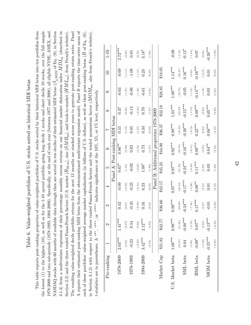
Table6.Value-weightedportfoliosofU.S.stockssortedonhistoricalMDIbetas
Thistablereportspost-rankingpropertiesofvalue-weightedportfoliosofU.S.stockssortedbytheirhistoricalMDIbetasintotenportfoliosfrom
thelowest(1)tothehighest(10),aswellasforthe1-10spreadportfoliogoinglongdecile1stocksandshortdecile10stocks,overthefullsample
1978-2009andtwosub-periods(1978-1993,1994-2009).Specifically,attheendofeachyear(between1977and2008),alleligibleNYSE,AMEX,and
NASDAQstockswith60monthsofavailabledatathroughthenaresortedintendecilesoftheirestimatedMDIbetas( βj,MDIofEq.(9),inSection
3.1.3)from
amultivariateregressionoftheirpercentagemonthlyexcessreturnsonourfinancialmarketdislocationindexMDI m
(describedin
Section2.2)andthethreetradedFama-Frenchfactors(U.S.market[ RM,m],size[SMBm],andbook-to-market[HMLm],from
French’swebsite).
Theresultingvalue-weighteddecileportfolioreturnsforthenext12monthsarestackedacrossyearstogeneratepost-rankingreturnseries.Panel
Areportstheirestimatedpost-rankingMDIbetasfrom
theaforementionedmultivariateregressionmodel.PanelBreportsthetime-seriesmeanof
eachoftheseportfolios’value-weightedaveragemarketcapitalization(inbillionsofU.S.dollars),aswellastheirpost-rankingbetas( B
ofEq.(6),
inSection3.1.2)withrespecttothethreetradedFama-Frenchfactorsandthetradedmomentumfactor( MOMm,alsofrom
French’swebsite).
t-statisticsareinparentheses.A“∗”,“∗∗ ”,or“∗∗∗”indicatessignificanceatthe10%,5%,or1%
level,respectively.
Pre-ranking
12
34
56
78
910
1-10
PanelA:Post-rankingMDIbetas
1978-2009
2.03∗∗∗
1.41∗∗∗
0.42
-0.09
0.67∗
0.86∗∗
0.55
0.37
-0.63
-0.69
2.72∗∗∗
(2.94)
(2.87)
(0.87)
(-0.22)
(1.78)
(2.30)
(1.19)
(0.96)
(-1.37)
(-1.11)
(2.64)
1978-1993
-0.23
0.54
-0.45
-0.25
-0.02
0.62
0.85
-0.14
-0.86
-1.08
0.85
(-0.23)
(0.66)
(-0.59)
(-0.44)
(-0.04)
(1.10)
(1.25)
(-0.24)
(-1.26)
(-1.31)
(0.56)
1994-2009
3.42∗∗∗
2.12∗∗∗
0.16
0.23
1.08∗
0.73
0.34
0.70
-0.61
0.23
3.18∗
(3.23)
(2.92)
(0.22)
(0.33)
(1.89)
(1.27)
(0.52)
(1.21)
(-0.85)
(0.22)
(1.94)
PanelB:Additionalproperties1978-2009
MarketCap
$21.82
$42.77
$36.66
$43.17
$45.25
$44.90
$36.37
$32.18
$28.85
$18.05
U.S.Marketbeta
1.08∗∗∗
0.98∗∗∗
0.98∗∗∗
0.97∗∗∗
0.97∗∗∗
0.92∗∗∗
0.98∗∗∗
1.01∗∗∗
1.00∗∗∗
1.14∗∗∗
-0.06
(34.27)
(41.65)
(40.60)
(46.44)
(51.30)
(49.78)
(43.43)
(52.33)
(43.73)
(36.37)
(-1.16)
SMLbeta
0.04
-0.08∗∗∗
-0.24∗∗∗
-0.17∗∗∗
-0.24∗∗∗
-0.16∗∗∗
-0.20∗∗∗
-0.15∗∗∗
-0.05
0.16∗∗∗
-0.12∗
(1.00)
(-2.70)
(-7.48)
(-5.96)
(-9.49)
(-6.51)
(-6.73)
(-5.74)
(-1.54)
(3.95)
(-1.85)
HMLbeta
-0.09∗
0.07∗∗
0.17∗∗∗
0.08∗∗
0.11∗∗∗
0.09∗∗∗
0.22∗∗∗
0.09∗∗∗
-0.14∗∗∗
-0.16∗∗∗
0.07
(-1.93)
(2.03)
(4.81)
(2.41)
(3.98)
(3.25)
(6.62)
(3.02)
(-4.16)
(-3.47)
(0.96)
MOMbeta
-0.25∗∗∗
-0.13∗∗∗
-0.01
0.01
0.03
0.04∗∗
0.08∗∗∗
0.05∗∗∗
0.03
0.01
-0.26∗∗∗
(-8.95)
(-6.42)
(-0.69)
(0.70)
(1.63)
(2.52)
(4.10)
(2.88)
(1.64)
(0.33)
(-5.89)
42

Table7.Alphasofvalue-weightedportfoliosofU.S.stockssortedonhistoricalMDIbetas
Thistablereportsannualizedintercepts(percentagealphas,multipliedby12)from
theregressionofmonthlyexcesspost-rankingreturnsof
twelve-monthvalue-weightedportfoliosconstructedbysortingU.S.stocksbytheirpre-ranking,60-monthhistoricalMDIbetas(seeSection3.1.3)on
theU.S.marketfactor( R
M,m,CAPM),thethreetradedFama-Frenchfactors(U.S.marketplussize[SMBm]andbook-to-market[HMLm]),or
thefourtradedfactors(Fama-Frenchfactorsplusmomentum[ MOMm]).Thetablealsoreportstheseportfolios’annualizedrawpercentageexcess
returns.t-statisticsareinparentheses.A“∗”,“∗∗ ”,or“∗∗∗”indicatessignificanceatthe10%,5%,or1%
level,respectively.
Pre-ranking
12
34
56
78
910
1-10
1978-2009
Raw
return
10.25∗∗∗
7.10∗∗
7.17∗∗
5.59∗∗
6.13∗∗
7.95∗∗∗
6.78∗∗
7.15∗∗
7.68∗∗
5.98
4.27∗
(2.87)
(2.41)
(2.54)
(2.00)
(2.26)
(3.06)
(2.46)
(2.49)
(2.48)
(1.60)
(1.70)
CAPMalpha
2.93∗
0.90
1.35
-0.40
0.34
2.34∗∗
1.05
0.90
0.98
-1.92
4.85∗
(1.75)
(0.73)
(1.03)
(-0.38)
(0.32)
(2.43)
(0.85)
(0.91)
(0.87)
(-1.23)
(1.92)
Fama-Frenchalpha
2.97∗
0.41
0.70
-0.57
0.15
2.22∗∗
0.30
0.75
1.89∗
-1.26
4.24∗
(1.74)
(0.34)
(0.59)
(-0.57)
(0.16)
(2.43)
(0.27)
(0.79)
(1.69)
(-0.83)
(1.67)
4-factoralpha
5.83∗∗∗
1.96∗
0.88
-0.72
-0.11
1.81∗
-0.58
0.23
1.49
-1.40
7.23∗∗∗
(3.70)
(1.67)
(0.74)
(-0.70)
(-0.12)
(1.95)
(-0.51)
(0.24)
(1.31)
(-0.90)
(2.92)
1978-1993
Raw
return
7.58∗
6.39
6.10
6.76∗
7.67∗
8.63∗∗
9.40∗∗
8.95∗∗
9.63∗∗
9.51∗
-1.93
(1.70)
(1.59)
(1.55)
(1.79)
(1.94)
(2.27)
(2.29)
(2.10)
(2.20)
(1.90)
(-0.65)
CAPMalpha
-0.24
-0.81
-1.01
-0.22
0.29
1.51
1.80
0.95
1.47
0.26
-0.50
(-0.12)
(-0.50)
(-0.68)
(-0.18)
(0.25)
(1.37)
(1.36)
(0.81)
(1.11)
(0.16)
(-0.17)
Fama-Frenchalpha
-0.64
-1.22
-1.26
-0.45
0.55
1.37
1.93
1.57
2.16
1.03
-1.67
(-0.32)
(-0.76)
(-0.84)
(-0.40)
(0.49)
(1.23)
(1.43)
(1.35)
(1.58)
(0.63)
(-0.56)
4-factoralpha
1.78
1.13
0.28
-0.73
0.35
0.62
0.34
1.11
1.75
-0.12
1.90
(0.89)
(0.73)
(0.19)
(-0.63)
(0.30)
(0.54)
(0.25)
(0.92)
(1.24)
(-0.07)
(0.65)
1994-2009
Raw
return
12.92∗∗
7.80∗
8.25∗∗
4.43
4.59
7.27∗∗
4.16
5.34
5.74
2.45
10.48∗∗∗
(2.31)
(1.82)
(2.03)
(1.08)
(1.24)
(2.04)
(1.13)
(1.39)
(1.31)
(0.44)
(2.59)
CAPMalpha
6.36∗∗
2.63
3.63∗
-0.55
0.20
3.00∗
0.04
0.64
0.41
-4.07
10.42∗∗
(2.42)
(1.44)
(1.70)
(-0.32)
(0.12)
(1.95)
(0.02)
(0.42)
(0.23)
(-1.52)
(2.56)
Fama-Frenchalpha
6.64∗∗
2.09
2.93
-0.75
-0.14
2.91∗∗
-0.98
0.16
1.31
-3.59
10.23∗∗
(2.50)
(1.15)
(1.65)
(-0.45)
(-0.10)
(2.06)
(-0.61)
(0.11)
(0.74)
(-1.41)
(2.52)
4-factoralpha
9.06∗∗∗
3.26∗
2.71
-0.85
-0.15
2.86∗∗
-1.19
-0.06
1.05
-3.37
12.44∗∗∗
(3.75)
(1.88)
(1.51)
(-0.50)
(-0.11)
(2.00)
(-0.73)
(-0.04)
(0.59)
(-1.31)
(3.14)
43

Table8.MDIbetasandalphasofequal-weightedportfoliosofU.S.stockssortedonhistoricalMDIbetas
Thistablereportsannualizedintercepts(percentagealphas,multipliedby12)from
theregressionofmonthlyexcesspost-rankingreturnsof
twelve-monthequal-weightedportfoliosconstructedbysortingU.S.stocksbytheirpre-ranking,60-monthhistoricalMDIbetas(seeSection3.1.3)on
theU.S.marketfactor( R
M,m,CAPM),thethreetradedFama-Frenchfactors(U.S.marketplussize[SMBm]andbook-to-market[HMLm]),or
thefourtradedfactors(Fama-Frenchfactorsplusmomentum[ MOMm]).Thetablealsoreportstheseportfolios’post-rankingMDIbetasfrom
the
aforementionedFama-Frenchmultivariateregressionmodel.t-statisticsareinparentheses.A“∗”,“∗∗ ”,or“∗∗∗”indicatessignificanceatthe10%,
5%,or1%
level,respectively.
Pre-ranking
12
34
56
78
910
1-10
1978-2009
Post-rankingMDIbeta
2.67∗∗∗
1.95∗∗∗
1.52∗∗∗
1.69∗∗∗
1.05∗∗∗
1.40∗∗∗
1.51∗∗∗
1.59∗∗∗
1.10∗∗∗
0.88∗
1.79∗∗∗
(5.12)
(4.52)
(3.75)
(4.82)
(2.94)
(4.27)
(3.51)
(3.97)
(2.77)
(1.90)
(2.66)
CAPMalpha
5.37∗∗∗
3.76∗∗∗
3.92∗∗∗
3.72∗∗∗
3.78∗∗∗
4.48∗∗∗
3.79∗∗∗
2.98∗∗
4.04∗∗∗
1.31
4.06∗∗
(3.29)
(2.85)
(3.23)
(3.37)
(3.39)
(4.18)
(3.04)
(2.53)
(3.28)
(0.82)
(2.39)
Fama-Frenchalpha
2.94∗∗
1.16
1.47
1.30
1.25
2.01∗∗
1.37
0.75
2.00∗∗
0.01
2.93∗
(2.24)
(1.08)
(1.46)
(1.47)
(1.42)
(2.46)
(1.29)
(0.76)
(2.04)
(0.01)
(1.77)
4-factoralpha
5.42∗∗∗
2.94∗∗∗
2.85∗∗∗
2.18∗∗
1.88∗∗
2.49∗∗∗
1.98∗
0.99
2.45∗∗
1.14
4.28∗∗∗
(4.59)
(2.94)
(2.95)
(2.50)
(2.13)
(3.03)
(1.84)
(0.98)
(2.46)
(1.01)
(2.59)
1978-1993
Post-rankingMDIbeta
1.11
0.39
0.10
0.90∗
0.51
0.53
0.62
-0.19
0.41
-0.32
1.42
(1.44)
(0.65)
(0.17)
(1.82)
(1.07)
(1.16)
(1.27)
(-0.39)
(0.76)
(-0.50)
(1.44)
CAPMalpha
1.57
1.33
1.72
2.88∗∗∗
3.20∗∗∗
3.75∗∗∗
3.23∗∗∗
0.91
4.21∗∗∗
1.65
-0.08
(0.85)
(0.98)
(1.25)
(2.61)
(3.10)
(3.29)
(2.80)
(0.81)
(3.25)
(0.94)
(-0.04)
Fama-Frenchalpha
-0.08
0.02
0.16
1.27
1.88∗∗
1.78∗
1.79∗
0.05
3.28∗∗∗
1.09
-1.17
(-0.05)
(0.02)
(0.13)
(1.28)
(1.98)
(1.94)
(1.85)
(0.05)
(3.10)
(0.88)
(-0.59)
4-factoralpha
2.78∗∗
2.65∗∗∗
2.27∗∗
2.79∗∗∗
3.21∗∗∗
2.79∗∗∗
2.15∗∗
0.79
3.88∗∗∗
1.47
1.32
(2.00)
(2.60)
(2.02)
(2.96)
(3.47)
(3.06)
(2.15)
(0.79)
(3.56)
(1.13)
(0.68)
1994-2009
Post-rankingMDIbeta
3.32∗∗∗
2.78∗∗∗
2.05∗∗∗
2.38∗∗∗
1.41∗∗∗
1.89∗∗∗
1.88∗∗∗
2.17∗∗∗
1.70∗∗∗
2.13∗∗∗
1.19
(4.08)
(4.33)
(3.46)
(4.53)
(2.73)
(3.91)
(2.88)
(4.16)
(3.01)
(2.80)
(1.10)
CAPMalpha
9.11∗∗∗
6.09∗∗∗
6.03∗∗∗
4.43∗∗
4.21∗∗
5.04∗∗∗
4.05∗
4.68∗∗
3.60∗
0.98
8.13∗∗∗
(3.42)
(2.70)
(3.03)
(2.33)
(2.16)
(2.82)
(1.92)
(2.45)
(1.79)
(0.36)
(2.95)
Fama-Frenchalpha
6.52∗∗∗
3.14∗
3.45∗∗
1.82
1.36
2.52∗∗
1.42
2.00
1.18
-0.57
7.08∗∗∗
(3.15)
(1.91)
(2.30)
(1.35)
(1.06)
(2.05)
(0.87)
(1.51)
(0.83)
(-0.30)
(2.68)
4-factoralpha
8.78∗∗∗
4.67∗∗∗
4.60∗∗∗
2.66∗∗
1.97
3.09∗∗
2.54
2.58∗∗
1.98
0.75
8.03∗∗∗
(4.93)
(3.14)
(3.27)
(2.03)
(1.55)
(2.55)
(1.63)
(1.96)
(1.44)
(0.42)
(3.05)
44

Table9.MDIriskpremiums:U.S.stocks
ThistablereportsestimatesofannualizedpercentageMDIriskpremiums(λMDI,multipliedby12)formultivariateMDIbetas(βi,MDI)of
value-weighted(PanelA)andequal-weighted(PanelB)portfoliosconstructedbysortingU.S.stocksbytheirpre-ranking,60-monthhistoricalMDI
betas(fromthelowest[decile1]tothehighest[decile10],seeSection3.1.3).Specifically,thetablereportsGMMestimatesofλMDIwhenaccounting
forthesensitivityoftheseportfolios’excessreturnstothethreetradedFama-Frenchfactors(U.S.market[ RM,m],size[SMBm],andbook-to-market
[ HMLm])orthefourtradedfactors(Fama-Frenchfactorsplusmomentum[MOMm])inEqs.(6)to(8)(inSection3.1.2),overthefullsample
1978-2009andtwosub-periods(1978-1993,1994-2009).WealsoreportestimatesofriskpremiumsperaverageMDIbeta( λMDIβi,MDI)andforthe
1-10spreadportfolio(goinglongdecile1stocksandshortdecile10stocks,λ
MDI
¡ β1,MDI−
β10,MDI
¢ ).Asymptotict-statisticsareinparentheses.
J-testistheasymptoticchi-squarestatisticfortheover-identifyingrestrictioninEq.(8);thecorrespondingp-valuesarebelow.A“∗”,“∗∗ ”,or“∗∗∗”
indicatessignificanceatthe10%,5%,or1%
level,respectively.
1978-2009
1978-1993
1994-2009
Fama-French
Four-factor
Fama-French
Four-factor
Fama-French
Four-factor
PanelA:Value-weightedportfolios
λMDI
1.58∗∗∗
2.89∗∗∗
-0.73
-23.06
1.38∗∗∗
2.74∗∗∗
(3.55)
(3.57)
(-0.93)
(-0.31)
(2.95)
(3.30)
λMDIβi,MDI
0.69∗∗
0.80∗∗∗
0.16
0.72∗∗
1.03∗∗
1.16∗∗
(2.53)
(2.64)
(0.92)
(2.41)
(2.18)
(2.34)
λMDI
¡ β1,MDI−
β10,MDI
¢4.36∗∗
7.15∗∗
-0.90
2.94
5.98∗∗
10.57∗∗∗
(2.18)
(2.96)
(-0.68)
(1.07)
(1.99)
(2.97)
J-test
10.93
10.16
4.94
6.57
11.64
7.29
0.28
0.34
0.84
0.68
0.23
0.61
PanelB:Equal-weightedportfolios
λMDI
0.95∗∗
2.17∗∗∗
3.19∗∗
3.31∗∗
1.18∗∗∗
2.27∗∗∗
(2.58)
(3.79)
(2.26)
(2.56)
(2.84)
(3.12)
λMDIβi,MDI
1.40∗∗
2.30∗∗∗
1.30∗
1.99∗∗
2.36∗∗
2.90∗∗∗
(2.23)
(3.81)
(1.75)
(2.40)
(2.37)
(3.12)
λMDI
¡ β1,MDI−
β10,MDI
¢1.89∗
3.70∗∗
-0.30
1.05
2.35
4.04∗
(1.77)
(2.35)
(-0.17)
(0.57)
(1.49)
(1.94)
J-test
10.02
10.09
6.48
4.96
12.24
10.92
0.35
0.34
0.69
0.84
0.20
0.28
45

Table10.MDIbetasandriskpremiums:Currencyportfolios
ThistablereportsOLSestimatesofunivariateMDIbetasβi,MDI,theslopecoefficientsfrom
time-seriesregressionsofpercentagemonthlyexcess
returnsofeachofthe8currencyportfoliosiinLustigetal.(2011)onMDI m,thefinancialmarketdislocationindexdescribedinSection2.2(Eq.
(4)inSection3.1.1),overthefullsampleperiodNovember1973-December2009(314observations)andtwosub-periods(1983-1993,1994-2009).The
sampleincludessixcurrencyportfoliosformedoninterestrates,from
low(1)tohigh(6),aswellasaportfoliogoinglongabasketofdevelopedand
emergingcurrenciesagainstthedollar( RX)andacarrytradeportfolio(HMLFX)goinglonghigh-interestratecurrenciesandshortlow-interest
ratecurrencies,from
Verdelhan’swebsite.ThetablealsoreportsOLSestimatesofλ0andthepercentageMDIriskpremiumsλMDI(annualized,
i.e.,multipliedby12)from
regressingcurrencyportfolios’meanexcesspercentagemonthlyreturnsRi,monthosepreviouslyestimatedunivariate
MDIbetas
βi,MDI(Eq.(5),inSection3.1.1),aswellastheriskpremiumperaverageMDIbeta(λMDIβi,MDI).R2 aistheadjustedR2.t-statistics
areinparentheses.A“∗”,“∗∗ ”,or“∗∗∗”indicatessignificanceatthe10%,5%,or1%
level,respectively.
OLSestimatesofMDIbetas
βi,MDI
MDIriskpremiums
12
34
56
RX
HMLFX
λ0
λMDI
λMDIβi,MDI
R2 a
1983-2009
0.09
-1.01∗
-0.43
-0.83
-1.30∗∗
-2.21∗∗∗
-0.95∗
-2.30∗∗∗
-0.86
-2.38∗∗∗
2.66∗∗∗
71%
(0.14)
(-1.81)
(0.75)
(-1.45)
(-2.05)
(-3.08)
(-1.82)
(-3.45)
(-1.13)
(-4.24)
(3.28)
1983-1993
1.50
1.96
0.91
0.41
1.47
0.23
1.08
-1.26
2.64∗∗∗
-0.82
-0.65
20%
(0.93)
(1.35)
(0.59)
(0.26)
(0.85)
(0.13)
(0.77)
(-0.78)
(4.31)
(-1.65)
(-0.46)
1994-2009
-0.01
-1.91∗∗∗
-0.99
-1.23∗∗
-2.41∗∗∗
-3.69∗∗∗
-1.71∗∗∗
-3.67∗∗∗
-2.05
-1.91∗∗∗
3.73∗∗∗
66%
(-0.02)
(-3.07)
(-1.57)
(-2.10)
(-3.64)
(-4.50)
(-3.04)
(-4.68)
(-1.79)
(-3.82)
(3.30)
46

Table11.MDIandstockreturnpredictability
ThistablereportssummarystatisticsfortheestimatedcoefficientsofOLSregressionsofone-month-aheadpercentageexcessreturns(R
i,m,m+1,
PanelA)orsix-month-aheadcumulativepercentageexcessreturns( R
i,m,m+6,PanelB)ofeachof26U.S.stockportfoliosiformedonsizeandbook-
to-market(oreachof50internationalstockportfoliosi)ontheirpreviousmonth’sexcessreturns(R
i,m,m)ortheirprevioussix-monthcumulative
excessreturns( R
i,m−6,m),respectively,andpreviousmonth’srealizationofthefinancialmarketdislocationindexdescribedinSection2.2(MDI m).
Specifically,wecomputeandreportsummarystatisticsfortheaforementionedregressions’coefficientsforMDI m
(δh=1
i,MDIandδh=6
i,MDIofEq.(10),
estimatedoverthelongestspanofavailabledatawithinthefullsample1973-2009andtwosub-periods[1973-1993,1994-2009]),multipliedbythe
correspondingin-samplestandarddeviationofMDI m
(i.e.,δh i,MDIσMDI),aswellasfortheirNewey-Westt-statistics(insquarebrackets).Because
ofdataavailability,δh i,MDIcannotbeestimatedforCzechRepublic,Egypt,Hungary,Morocco,andRussiaover1973-1993.N∗isthenumberof
portfoliosforwhich
δh i,MDIissignificantatthe10%levelorless;δ∗ iσisthecorrespondingaverageδh i,MDIσMDI(withaveraget-statisticsinsquare
brackets);R2∗aisthecorrespondingaverageadjustedR2.Fortheminimum
andmaximum
δh i,MDIσMDI,actualt-statisticsareinparentheses.
PanelA:One-month-aheadexcessreturns
PanelB:Six-month-aheadcumulativeexcessreturns
Estimated
δh=1
i,MDItimes
σMDI
Estimated
δh=6
i,MDItimes
σMDI
Mean
Median
Stdev
Min
Max
N∗
δ∗ iσ
R2∗a
Mean
Median
Stdev
Min
Max
N∗
δ∗ iσ
R2∗a
U.S.plus25U.S.portfolios
U.S.plus25U.S.portfolios
1973-2009
-0.27
-0.25
0.11
-0.55
-0.11
1-0.55
1.21%
0.53
0.58
0.80
-0.77
2.38
22.32
1.56%
[-0.79]
[-0.73]
[0.34]
(-1.69)
(-0.26)
[-1.69]
[0.45]
[0.55]
[0.70]
(-0.83)
(1.72)
[1.82]
1973-1993
0.01
0.00
0.00
-0.25
0.28
0n.a.
n.a.
1.43
1.46
1.46
0.24
2.80
0n.a.
n.a.
[0.05]
[0.01]
[0.01]
(-0.47)
(0.93)
[n.a.]
[1.01]
[1.06]
[1.06]
(0.22)
(1.37)
[n.a.]
1994-2009
-0.59
-0.61
0.23
-1.15
-0.13
4-0.82
3.70%
0.23
-0.08
1.25
-1.89
3.28
23.05
1.37%
[-1.18]
[-1.14]
[0.53]
(-2.49)
(-0.17)
[-2.01]
[0.09]
[-0.07]
[0.89]
(-1.40)
(1.74)
[1.79]
Worldplus49countryportfolios
Worldplus49countryportfolios
1973-2009
-0.58
-0.44
0.57
-2.16
0.54
14-1.16
3.08%
-0.09
-0.14
2.80
-7.95
6.19
13-1.19
3.78%
[-1.02]
[-0.92]
[0.97]
(-2.04)
(0.81)
[-2.22]
[-0.18]
[-0.09]
[1.38]
(-2.61)
(2.85)
[-0.92]
1973-1993
-0.51
-0.41
2.30
-8.41
8.71
14-1.47
10.12%
-2.25
-2.46
4.85
-17.61
6.81
19-4.46
9.86%
[-0.69]
[-0.59]
[1.48]
(-4.32)
(0.97)
[-1.57]
[-1.23]
[-1.23]
[1.75]
(-2.64)
(1.69)
[-2.34]
1994-2009
-0.49
-0.57
0.60
-2.16
1.01
10-0.93
4.75%
0.46
-0.07
3.23
-7.95
8.44
111.09
4.05%
[-0.79]
[-0.84]
[0.99]
(-2.04)
(1.72)
[-1.82]
[0.06]
[-0.03]
[1.42]
(-2.61)
(2.46)
[0.11]
47

Table 12. MDI and currency return predictability
This table reports the estimated predictive coefficients of OLS regressions of one-month-ahead percentage
excess returns (Ri,m,m+1, Panel A) or six-month-ahead cumulative percentage excess returns (Ri,m,m+6, PanelB) of each of the 8 currency portfolios i described in Section 3.2 (six currency portfolios formed on interest rates,from low [1] to high [6], as well as a portfolio going long a basket of developed and emerging currencies against
the dollar [RX] and a carry trade portfolio [HMLFX ] going long high-interest rate currencies and short low-interest rate currencies) on their previous month’s excess returns (Ri,m,m) or their previous six-month cumulativeexcess returns (Ri,m−6,m), respectively, and previous month’s realization of the financial market dislocation indexdescribed in Section 2.2 (MDIm). Specifically, we report the aforementioned regressions’ coefficients forMDIm(δh=1i,MDI and δ
h=6i,MDI of Eq. (10), estimated over the full sample 1983-2009 and two sub-periods [1983-1993, 1994-
2009]), multiplied by the corresponding in-sample standard deviation ofMDIm (i.e., δhi,MDIσMDI), as well asfor their Newey-West t-statistics (in parentheses). R2a is the corresponding adjusted R
2. A “∗”, “∗∗”, or “∗∗∗”
indicates significance at the 10%, 5%, or 1% level, respectively.
1 2 3 4 5 6 RX HMLFXPanel A: One-month-ahead excess returns
Estimated δh=1i,MDI times σMDI1983-2009 -0.21 -0.27∗∗ -0.24∗ -0.22 -0.24∗ -0.04 -0.21 0.17
(-1.11) (-2 .18) (-1 .72) (-1 .55) (-1 .67) (-0 .19) (-1 .51) (0 .93)
R2a 0.11% 1.50% 0.51% 2.18% 3.18% 1.86% 1.46% 2.05%
1983-1993 -0.34 -0.19 -0.42∗ -0.20 -0.07 -0.02 -0.21 0.36
(-1.23) (-0 .87) (-1 .78) (-0 .74) (-0 .28) (-0 .06) (-0 .92) (1 .57)
R2a 0.38% -1.04% 0.99% -0.55% -0.85% 0.10% -0.81% 1.10%
1994-2009 -0.11 -0.24∗ -0.19 -0.20 -0.28∗ -0.06 -0.18 0.06
(-0.45) (-1 .70) (-1 .14) (-1 .23) (-1 .77) (-0 .23) (-1 .08) (0 .28)
R2a -0.31% 3.08% 0.04% 4.92% 7.84% 2.18% 3.44% 2.34%
Panel B: Six-month-ahead cumulative excess returnsEstimated δh=6i,MDI times σMDI
1983-2009 -0.92 -0.91∗ -0.24 -0.95∗ -0.26 0.20 -1.71 1.22
(-1.46) (-1 .76) (-0 .48) (-1 .66) (-0 .42) (0 .34) (-0 .94) (1 .51)
R2a 4.06% 2.51% 0.50% 3.14% -0.51% 0.06% 1.26% 1.34%
1983-1993 -2.38∗∗ -1.20 -2.05∗∗ -2.40∗∗ -0.68 -1.31 -1.71∗∗ 1.22
(-2.34) (-1 .53) (-2 .20) (-2 .42) (-0 .76) (-1 .32) (-1 .98) (1 .62)
R2a 14.89% 2.31% 7.21% 8.54% -1.04% 0.83% 5.78% 1.00%
1994-2009 0.16 -0.45 0.47 0.15 0.28 0.96 0.31 0.29
(0.34) (-0 .91) (1 .05) (0 .30) (0 .49) (1 .48) (0 .67) (0 .38)
R2a -0.89% 0.14% 1.69% 5.33% -0.49% 1.59% 0.86% -0.27%
48

Figure1.Arbitrageviolations
Thisfigureplotsmonthlyaveragesofdailyequal-weightedmeansofobservedabsolutelogno-arbitrageviolations(inbasispoints,i.e.,multiplied
by10,000)across63permutationsoftheCoveredInterestRateParitydescribedinSection2.1.1( CIRPm,inFigure1a,over236monthsm),across
122permutationsoftheTriangularArbitrageParitydescribedinSection2.1.2( TAPm,inFigure1b,over444months),andacross410permutations
oftheADRParitydescribedinSection2.1.3( ADRPm,inFigure1c,over441months),betweenJanuary1973andDecember2009.
a)CIRParbitrage(CIRPm,inbps)
b)Triangulararbitrage(TAPm,inbps)
c)ADRarbitrage(ADRPm,inbps)
0102030405060708090
1973
1975
1977
1979
1981
1983
1985
1987
1989
1991
1993
1995
1997
1999
2001
2003
2005
2007
2009
Month
0
0.01
0.02
0.03
0.04
0.05
0.06
0.07
0.08
0.090.1
1973
1975
1977
1979
1981
1983
1985
1987
1989
1991
1993
1995
1997
1999
2001
2003
2005
2007
2009
Month
0
100
200
300
400
500
600
700
1973
1975
1977
1979
1981
1983
1985
1987
1989
1991
1993
1995
1997
1999
2001
2003
2005
2007
2009
Month
49

Figure 2. The market dislocation index
This figure plots the Market Dislocation Index described in Section 2.2 (MDIm). The index is constructedas a monthly average of equal-weighted means of daily abnormal (i.e., standardized), absolute log no-arbitrage
violations (in basis points, i.e., multiplied by 10,000) across 63 permutations of the Covered Interest Rate Parity
described in Section 2.1.1 (CIRP zi,m), 122 permutations of the Triangular Arbitrage Parity described in Section2.1.2 (TAP zi,m), and 410 permutations of the ADR Parity described in Section 2.1.3 (ADRP zi,m), betweenJanuary 1973 and December 2009. Each individual absolute log difference between actual and theoretical prices
is standardized by its historical mean and standard deviation over at least 22 observations up to (and including)
its current realization.
Market dislocation index (MDIm)
‐1
‐0.5
0
0.5
1
1.5
1973
1975
1977
1979
1981
1983
1985
1987
1989
1991
1993
1995
1997
1999
2001
2003
2005
2007
2009
Month
50

Figure3.MDIbetasandstockandcurrencyportfolios’excessreturns
Thisfigurepresentsscatterplotsofannualizedmeanpercentageexcessstockandcurrencyreturns(i.e.,multipliedby12,rightaxis)versus
theirfinancialmarketdislocationriskbetas( βi,MDI)estimatedinEq.(4).Figure3aisbasedon26U.S.stockportfolios:ThebroadU.S.market
(thelargest,circularscatter)and25portfoliosattheintersectionoffiveportfoliosformedonsize(marketequity)andfiveportfoliosformedon
book-to-market(bookequitydividedbymarketequity),from
French’swebsite.MDIbetasandmeanexcessreturnsareestimatedforeachU.S.
portfoliooverthefullsample1973-2009.Figure3bisbasedon50internationalstockportfolios:Theworldmarket(thelargest,circularscatter),23
developed,and26emergingmarketportfolios,from
MSCI.MDIbetasandmeanexcessreturnsareestimatedforeachcountryoverthelongestspan
ofavailabledatawithinthefullsample1973-2009.Figure3cisbasedon8currencyportfolios:sixportfoliosformedoninterestrates,aportfolio
goinglongabasketofdevelopedandemergingcurrenciesagainstthedollar( RX),andacarrytradeportfoliogoinglonghigh-interestratecurrencies
andshortlow-interestratecurrencies( HMLFX,thelargest,circularscatter).MDIbetasandmeanexcessreturnsareestimatedforeachcurrency
portfoliooverthefullsample1983-2009.Scatterswithdark(white)backgroundrefertostatistically(in)significantMDIbetas,atthe10%levelor
less. a)
MDIbetasandU.S.stockreturns
b)MDIbetasandcountrystockreturns
c)MDIbetasandcurrencyreturns
0.00
2.00
4.00
6.00
8.00
10.00
12.00
14.00
‐4.50
‐4.00
‐3.50
‐3.00
‐2.50
‐2.00
‐1.50
‐1.00
MDI beta
Mean excess return
‐10.00‐5.000.00
5.00
10.00
15.00 ‐1
9.00
‐17.00
‐15.00
‐13.00
‐11.00
‐9.00
‐7.00
‐5.00
‐3.00
‐1.00
MDI beta
Mean excess return
‐2.00
‐1.000.00
1.00
2.00
3.00
4.00
5.00
6.00 ‐2.5
‐2‐1.5
‐1‐0.5
00.5
MDI beta
Mean excess return
51