Financial Market Assumptions & Models for Pension Plans:

A Technical Comment on the PIMS Model Assumptions for Asset Markets

Christopher C. Geczy

The Wharton School

University of Pennsylvania

This Draft: April 8, 2013

Correspondence to Christopher C. Geczy, Finance Dept., Wharton School, 3620 Locust Walk, Philadelphia PA,

19104; Phone 215-898-1698, e-mail geczy@wharton.upenn.edu. I thank Kyle Binder, Alimu Abudu, and Ankur

Dadhania for helpful research assistance. The research reported herein was pursuant to a grant from the U.S. Social

Security Administration (SSA) funded as part of the Retirement Research Consortium (RRC); the author also

acknowledges support from The Pension Research Council at The Wharton School. All findings and conclusions

expressed are solely those of the author and do not represent the views of the SSA or any agency of the federal

government, the MRRC, the PRC, or The Wharton School at the University of Pennsylvania.

ABSTRACT

Financial Market Assumptions & Models for Pension Plans:

A Technical Comment on the PIMS Model Assumptions for Asset Markets

The financial market assumptions of the PBGC’s PIMS model are critical inputs to simulations

for most apparent uses of the system. They currently appear to be based on a reduced form,

“classical” approach to assessing and forecasting the distribution of returns on various classes of

input assets, allowing for a fairly sophisticated and highly useful approach to understanding

simulated distributions of potential pension insurance outcomes as well as the net financial status

of the PBGC. This technical note discusses some of the capital market side assumptions utilized

in the model. It also comments on important related assumptions including the assumed asset

allocations of insured plans, making suggestion for possible modification of input assumptions of

the model to reflect time variation in financial market return behavior as well as time variation in

observed plan allocations.

1

1. Introduction and Scope

In this technical comment, we address a subset of the modeling assumptions of the PIMS

system developed and employed by the PBGC, focusing our attention on the capital market

expectations of asset classes assumed to represent holdings of plans insured by the agency as

well as those asset class allocation assumptions themselves. Examination of such suppositions

and their modeling implications can of course be important. However, we hasten to add that

without understanding or perhaps guessing about the implications of changes in assumptions, the

ultimate import of this examination is limited. That said, what follows represents an assessment

of a few of what we see as the most important assumptions for capital market behavior as well as

some apparent quickly moving industry trends that may also affect outputs and should be

addressed in the modeling assumptions of PIMS. While it seems logical that because

simulations can be sensitive to certain assumptions (and expected outputs are complex functions

of inputs) and because we view our comments as important both econometrically and as part of

powerful industry trends that are potentially important to PBGC outcomes, it is surely the case

that only when changes to the PIMS capital market and asset allocation assumptions are directly

incorporated in the model will we come to understand the actual importance of what follows.

Finally, it is highly worthwhile to note that the PBGC staff is likely to be aware of the ideas

outlined in the comment below and have indicated at various points in the system documentation

and associated literature that future versions of the system may include modifications

incorporating these ideas.

2. Overview of the PIMS Model Assumptions

The Pension Insurance Modeling System (PIMS) is a simulation modeling framework

developed by the Pension Benefit Guarantee Corporation (PBGC) that was “designed to quantify

the uncertainty that surrounds pension insurance” and to be used as a tool to characterize

potential distributions of pension insurance claims on the PBGC and, importantly, the agency’s

surplus (or deficit).1 The PBGC is clear that the system is not a predictive system intended to

identify point estimates of the future financial condition of the agency but to provide ranges of

simulated distributions of outcomes. (Ibid.). The system has been designed and maintained by

the agency (and, presumably, outside parties, contractors and other stakeholders via various

1 “Pension Insurance Modeling System: PIMS System Description,” Version 1.0, Revision 9/22/2010.

2

direct interactions with the model as well as via technical reviews such as this one and in other

ways) to give an understanding of how pension plans insured by the PBGC behave under various

shocks to internal and external parameters (which characterize economic and other conditions),

including being able to “accurately portray underfunding among the insured universe under a

wide variety of economic conditions” as long as the assumptions, constraints and reflections of

pension plan and governing rule data are accurate. Of course, modeling decisions about

granularity of the system components and data used and measured must have been made, and the

system cannot be possibly expected to capture all possible relevant inputs or reflect all possible

scenarios conceivable.

The system accommodates inputs from a subsample of large insured pensions including

actuarial inputs such as current plan demographics and benefit formulas, data on the financial

condition of sponsors, fund portfolio compositions and the PBGC’s own financial position.

We understand that, typically, PIMS simulations (say 5,000 or 10,000 in number of

draws over different economic scenarios) are used, say, to project 10 years of future economic

events in the financial markets (Overview, 2011). First, interest rates, stock returns, and related

variables (e.g., inflation, wage growth, and multiplier increases in flat-dollar plans) are drawn

according to the stochastic equations listed in Table 1. These variables are determined by interest

rates. In the model, the 30-year Treasury bond is presumed to follow a random walk while

corporate bond yields, which are highly correlated over time, are mean reverting to historical

estimates of their spread over Treasury yields of comparable maturity (VERIFY). Real rates are

calculated deterministically as an adjustment presuming a fixed inflation rate (e.g., 1.4%). The

term structure of interest rates does not enter into the equations (Overview, 2011).

Returns on equities are mean reverting to a long run average value estimated from

historical data (e.g., 10.4% plus noise according to one document or 8.6% or 8.2% according to

other documents) using data ranging from 1926, which is when the famous Stock, Bonds, Bills

and Inflation (SBBI) data from Ibbotson begin (PBGC, FY 2012 Exposure Report, hereafter

referred to as Exposure Report). Innovations are drawn IID over time, presumably from a

calibrated Gaussian distribution. Correlations between stock returns and bond yields are strictly

based on historical estimates from the time period 1973-2007 (Exposure Report), with the

implication being that of contemporaneous negative correlation between stocks and bonds. Plan

asset returns are determined by a two factor model that combines stock return premia over

3

nominal rates and bond premia, both adjusted for sensitivies to these premia via estimates of beta

a la a two factor market model. Note that in a one factor case, this model might be thought of as

the time series estimation equation made famous by the Capital Asset Pricing Model of Sharpe

(1964). It is important to note that the PBGC has indicated that it has Form 5500 data on

reported plan asset allocations, which in the future it might incorporate. My comments below on

the changing nature of plan allocations must be conditioned with this information. Asset mixes

of plan portfolios are assumed roughly to be a 60% allocation to equities and 40% allocation to

bonds (Buck Consulting, 2012) or “a weighting based on the average of the estimated rate

mixtures: 48 percent stock market returns, 23 percent long-term Treasury bond returns, 30

percent long-term Treasury bond yield and a -2.5 basis points additive adjustment.” (Exposure

Report)

Health and ultimately sponsor contributions first presume that sponsors make the

minimum statutory contributions implied by the tax code. If a sponsor goes bankrupt in the

simulation, it does not contribute from the previous year. The PBGC adjusts premia based on

sponsor historical choices to fund plans above the minimum in avoidance of higher premiums.

PIMS simulations allow plan participants to retire, leave the firm and to die according to

actuarial data and assumptions. Benefits and salaries for a given age and service time grow with

inflation plus a productivity factor (Overview, 2011 and see Table 1).

As mentioned above, sponsor health is measured by their equity-to-debt ratio, cash flow,

firm equity, and employment levels. Here, equity-to-debt and cash flow ratios are mean-

reverting to long run historical averages. Employment and firm equity are essentially modeled

as correlated random walks. Innovations in the equations for sponsors appearing in Table 1 are

assumed to be correlated to one another and to innovations in financial market returns, with

correlations estimated from history. Finally, bankruptcy is modeled as a random function with

parameters estimated by historical bankruptcies and data on the health of companies over the

period 1980 to 1998 (Exposure Report). These data are not industry-specific. If a firm goes

bankrupt at the same time a plan is less than 80% funded, the plan represents a loss and is

included in average loss calculations across simulations and scenarios (Exposure Report)

Discuss the excellent inclusion of parameter uncertainty in simulations. To Be

Completed.

4

3. PIMS Capital Market Assumptions vs. the Assumptions of Others

Table 2 outlines the capital market expectations use by the PIMS system. It also provides

a listing of the capital market assumptions recently compiled by Horizon Actuarial Services,

LLC in its annual survey of seventeen large multi-employer consultancies2. While the

assumptions utilized by plans insured by the PBGC are not available (at least to me), and the use

of third party capital market assumptions is fraught with its own problems, not the least of which

is the prima facie problem that that the respondents are service providers to plan sponsors and

are paid by them. However, it is reasonable to assume that when these advisors, as likely

fiduciaries under both the Advisors Act of 1940 and under ERISA, provide their expectations

which likely serve as a base for sponsor assumptions, these consultancies are required to provide

their advice in an un-conflicted manner as required under the law, and these consultancies advise

both single-employer and multi-employer plans in their fiduciary advisory capacities. Also, they

use a wide variety of models that are forward looking as well as historical data.

The results in Table 2a indicate a substantial discrepancy between the expected returns

used in the PIMS system (where we note that we have multiple sources describing the PIMS

assumptions)3 and large consultancies who likely serve the plans insured by the PBGC. Part of

the discrepancy surely arises directly from the fact that consultancies have different approaches

to assessing future capital market investment performance. Apparently, some use forward-

oriented models such as a form of the dividend discount model for equity returns. Certainly some

use historical data or at least calibrate their models based on historical data.

While information is sparse on how all seventeen consultancies compute their forecasts,

the importance of this discrepancy is that if plan sponsors base their allocations on them, and, as

a result, their allocations differ from the assumptions of the PBGC’s 60/40 presumption, extreme

differences might arise in PIMS simulations under the alternative. Also, the mere fact that

reasonable analysts can rely on different models for asset returns at least raises the chalice of

testing of robustness by the PBGC with respect to its own assumptions.

2 Consultancies included are Callan Associates, CAPTRUST Financial Advisors, A.J. Gallagher / Independent

Fiduciary Services, Hewitt EnnissKnupp, Investment Performance Services, LLC, R.V. Kuhns & Associates, Marco

Consulting Group, Marquette Associates, Meketa Investment Group, J.P. Morgan, Morgan Stanley/Graystone

Consulting, NEPC, Pension Consulting Alliance, The PFM Group, SEI Towers Watson and Wurts & Associates.

3 Here we use those model averages reported in the PBGC FY 2012 Exposure Report (2012). However, we also note

that the expected returns reported in the Buck Consultants third party review very closely resemble those appearing

in Table 2.

5

As we show in Section 5 below, evidence that corporate plans allocate much differently

than presumed by the PBGC seems undeniable. They allocate to more asset classes that are

represented in the U.S. 60/40 assumption, and some of those allocations are to classes of assets

that are highly likely to be exposed to risks simply outside the risks of U.S. domestic stocks and

bonds. Thus, as apparent in the unconditional expected returns, risks and correlations

assumptions presented in Table 2, higher volatilities for foreign classes and classes outside the

narrow confines of the PIMS assumption would likely result in higher volatilities and more

extreme outcomes, were the alterative presumptions to be more accurate. Moreover, since the

volatility attribution implied by the 60/40 assumption clearly indicates that this asset allocation,

which has arisen historically in the financial industry (and academic literature4) as a so-called

“balanced” portfolio, is in fact not at all balanced. Its risk is heavily dominated by the risk of the

equity component of the assumption. All this said, however, we hasten to add that the

assumptions of the average consultant may not accurately reflect the forecasts of reasonable

models. In Section 4 below, we turn to models that, in a forward looking way, calibrate market

expectations.

4. PIMS Capital Market Assumptions and the Stochastic Character of Asset Prices

Since no later than the work of Mandelbrot, Fama and others, the non-Gaussian character

of asset prices has been a topic of intense study in academia and industry. The gist of that body

of research and practice suggests that asset returns are have greater extremes than presumed by

the type of stochastic assumption embedded in the PIMS system. In addition, at least one source

of that heavy-tailed character is the time-varying nature and auto-correlated nature of first and

higher moments. The PIMS model assumptions on one hand incorporate a form of this

autocorrelation (e.g., the well-known autocorrelation of bond yields). On the other hand, they

appear to ignore the time-varying nature of volatility in the short and long runs.

There are numerous ways to illustrate this critical point. The approach we take here is

first to illustrate basic levels of predictability in asset returns. We do this graphically (Figures 1a

and 1b), although much research has demonstrated how reduced form and more structural

4 See for example, Brinson, Hood and Beebower (1986).

6

approaches may be estimated econometrically.5 We then make the point that volatility is time-

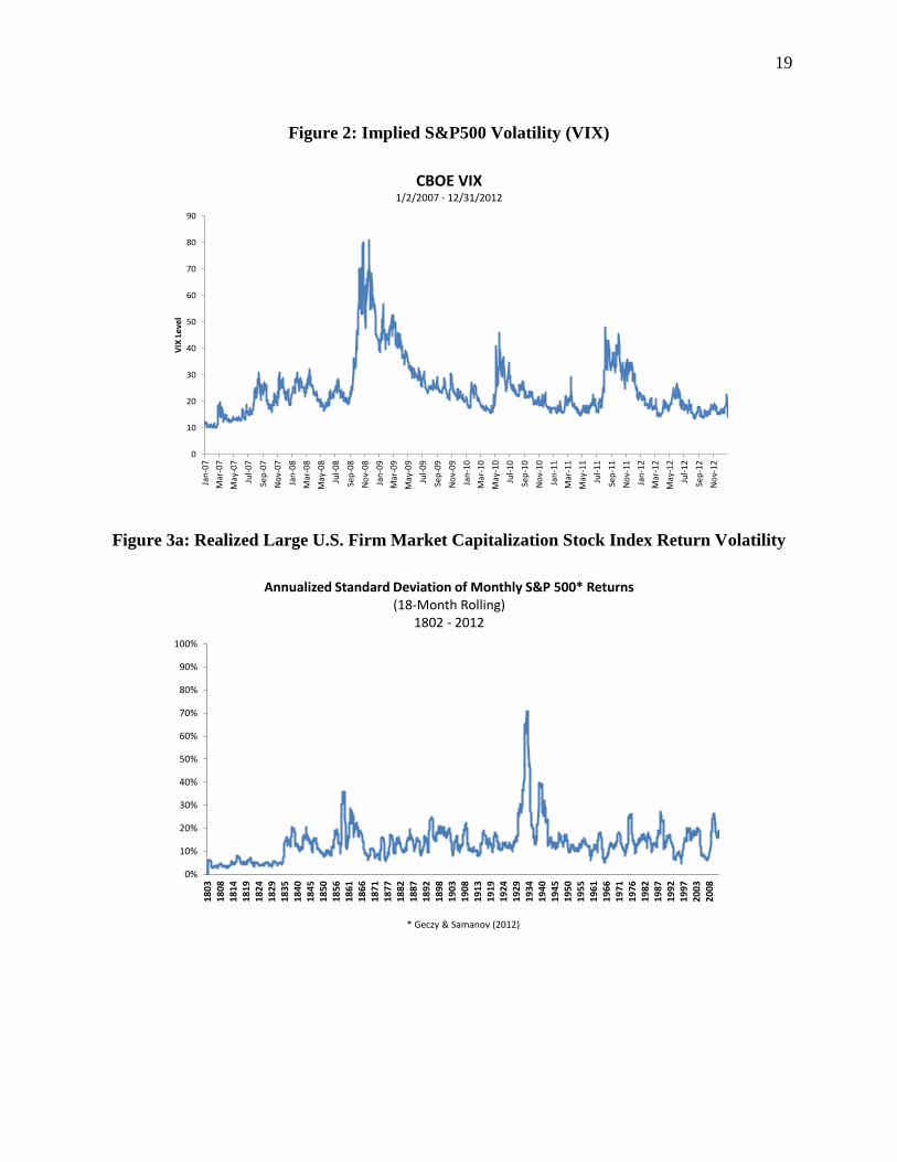
varying using implied volatilities (Figure 2), ex post realized volatilities over the long run

(Figures 3a and 3b), and, ultimately, using a simulation in which we employ a multivariate

E/GARCH approach, demonstrating the strongly different implications for the assumption of

time-varying volatility for outcomes with a greater frequency of extremes in simulations.

Since PBGC insurance both conceptually and as modeled in PIMS is expected to pay at

times when plans are underfunded and sponsors are in distress, having a more accurate

representation of equity market extremes seems quite important. Moreover, the diversification

benefits normally attributed to asset allocation varies with time and with market volatility. We

show below – again, graphically (Figures 4 and 5) – how the correlation between stocks and

bonds varies across both business and volatility cycles.

To illustrate the first point, Figure 1a relates starting 5-year Treasury yields (same axes)

to future annualized returns on Treasuries from January 1955 – January 2013, and Figure 1b

relates the current dividend yield on U.S. Large Cap stocks (reflected most recently in the S&P

500) over the period January 1871 – January 2013. Both graphs make two strong points, ones

that the academic literature has spent considerable effort in understanding over approximately

the last three decades. First, the graphs imply that it is impossible to assert that either equity

returns are simply random walks with IID innovations or that bond returns are simply mean

reverting with IID innovations. Second, the investment opportunity set is highly time-varying

and correlates strongly with simple instruments (for instance, the period correlation between d/p

and subsequent 7-year return in Figure 1b is just under 70%). Especially since insurance claims

are a strong function of these two forcing variables in the PIMS system and since they track

economic conditions, it may be useful to incorporate this notion into the assumptions of the

model.

Another feature of real-world data that today does not appear to be as controversial as it

was when first introduced is the property of asset returns to have fat tails and highly

autocorrelated conditional volatilities and time-varying implied volatilities that reflect the pricing

of systematic risk. Again, there may be innumerable ways to make this point, and one guesses

that there may be thousands of academic and practitioner papers and dissertations written on the

5 Although I hasten to add that some researchers like Welch (2008) indicate that much of the predictability

documented in the academic finance literature arises due to data mining.

7

topic, but we again here take a graphical approach (later we build a simulation model that

accommodates time-varying volatility). Figure 2 presents the Chicago Board of Options

Exchange VIX index over the period January 2007 – December 2012, and Figure 3a presents ex

post realized volatility estimated over 18-month rolling windows. Both graphs tell a similar story

of time-varying volatility with that variation corresponding to business and market cycles over a

recent period of market disruption and, in fact, in the very long run (at least by U.S. standards).

Moreover, ninety-nine percent of positive daily changes in the VIX index correlate with negative

S&P 500 index returns. That is, equity values are negatively correlated with increases in

volatility. Finally, over the long run, cycles like those apparent in the recent financial crisis are

reflected in realized volatility. Again, while sophisticated modeling assumptions and

technologies capturing this effect may take many different forms, the graphs point out clearly

that the modeling assumptions of the PIMS system may usefully incorporate conditional

heteroskedasticity in asset returns, or at least for equity returns.

To illustrate this point, Figure 3b incorporates our understanding of the PIMS equity

return assumptions from Table 1 in modeling simulated returns that are either random walks like

those from the PIMS model (which we label “IID”) or a calibrated random walk (cleverly

labeled “Calibrated”) using in-sample estimates of the period represented by each point on the

graph for actual returns. Apparent in this graph is that the actual spikes in volatility arising in the

real world are not reflected in the IID approach of the PIMS model estimated based on long-run,

constant variance assumptions. Moreover, while local calibration helps over the rolling horizons

of the model (and it should, as it benefits from perfect hindsight!), it is not able to match the

observed spikes in volatility in the historical record. The implication of these figures is that,

again, because volatility is so strongly inversely correlated with bad outcomes for asset

valuations, in our view a model of insurance may fruitfully incorporate these effects.

Unfortunately, it turns out that spikes in volatility due, in our view, both to characteristics

of asset returns themselves and possibly to ancillary effects (like runs on liquidity that arise

during financial crises and times of systemic stress, which have happened so commonly

throughout modern human history (e.g., see Kindleberger and Aliber, 2012)). One way among

many to understand this effect is to think simply how components of classes of assets like those

to which insured plans have exposure relate in their variations to the classes as a whole.

Consider, for example, the traditional portfolio theoretic measure, R2. The fundamental

8

definition of R2 for an asset in an investment context is as the ratio of its systematic (e.g.,

market) risk to its total risk which is the sum of systematic and idiosyncratic, non-market risk.

The previous figures indicate that the numerator and the first part of the denominator, systematic

or market risk, change over time and with widespread pricing of equity risk, and, at times, spike.

Unless idiosyncratic risk compensates for changes in systematic risk, R2s may vary as well.

Moreover, formulaically, R2 is defined as the square of correlation between the asset and the

asset class being modeled. That is, just when the diversification power of lower-than-higher

correlations are most important, they may be fleeting. Altogether, this indicates that just when

assumptions about constant correlations may be important, they may actually go up. This effect

may be especially important to the PBGC because sponsor contributions are functions of

financial distress of sponsor firms, which is likely correlated with shocks common to equities.

Even more, PBGC assets may themselves be subject to this behavior, making claims (and other

difficult outcomes) and their backstop move more negatively in bad times. To illustrate this

point, Figure 4 plots the implied correlations of the S&P 500 components via the term structure

of the futures contracts JCJ, KCJ and ICJ over time, in which it is notable that correlations

implied by options prices are both time-varying and correlated with volatility spikes in the

previous graphs. Finally, Figure 5 plots rolling realized correlations between and index of U.S.

large cap stocks (represented most recently by the S&P 500) with 20-year Treasury returns.

While the PIMS model assumptions presume a fairly strong negative correlation between stock

and bond returns, it is clear at least from the perspective of Figure 5, this presumption may be

appropriate only at certain times. However, it is quite important to note that the negative

observed correlation in Figure 5 often appears over estimation periods covering periods of

market distress, perhaps making the PIMS assumption tenable or appropriate. Nonetheless,

again, it may be useful for the PIMS system to incorporate time-varying second moments in a

multivariate context for asset returns, particularly if, as discussed in Section 5, the system would

be moving toward consideration of more asset classes than just the components of the 60/40

portfolio in plan allocations.

5. PIMS and Models for Capital Market Expectations

As the treatment in Section 2 above highlights, there exist strong differences between the

capital market assumptions for the simple asset classes of the PIMS model and the assumptions

9

of large consultancies assumed to be providing investment advice to the sponsors of insured

plans. To assess further the PIMS assumptions about equities, we estimate two additional

models for future asset returns, focusing on equity returns: The dividend discount model and a

model based upon dividend yield as an instrument which accommodates the time-varying nature

of expected returns in the academic and practitioner literature. With respect to future expected

returns on bonds, the evidence in Figures 1a and 1b relating yields to future returns over time

indicates that, based on the assumption of current yields being unbiased predictors of future

returns (an assailable presumption, but a reasonable one here as long as residual correlations are

maintained), future bond returns might actually be quite a bit lower than presumed by the PIMS

systems, based upon our assessment. While this indication is not a direct comment about the

modeling character of the system, it points out a difference that arises based upon modeling

choices of the system.

To Be Added in the Revision

6. Asset and Risk-Based Allocations of Pension Plans and Their Implications

In this section we demonstrate that the asset allocation of the PIMS system, which

presumes a 60%/40% stock/bond split, does not comport with the allocation of many plans today

or with trends in plan allocations and, thus, may not reflect the actual risk of plans on average.

The risks of those plans differ substantially from that of the so-called “balanced” approach of the

famous 60/40 allocation, which is in the PIMS model essentially a U.S.-based model. First,

Table 3 provides allocations across a fairly highly aggregated depiction of asset classes from

various sources in the PIMS documentation set as well as for U.S. corporate plans, U.S. public

plans and a sample of U.S. defined benefit plans (the largest 100 corporate plans in 2012),

according to Pensions & Investments Research (2013). The column labeled PIMS Model refers

to the allocations reported to me assumed in the Exposure Report, and the columns labeled

Single Employer Funds/Plans represent a summary and subjective aggregation of the allocations

reported in the PBGC Annual Report for 2012. The columns labeled as corporate and public

plans are also those that appear for 2011 in Figures 6a-6c from the P&I annual plan surveys.

Table 3 indicates that the U.S. 60/40 assumption is quite different from plan allocations

across the board which, largely and recently, have lower levels of equity allocations than the

assumption of PIMS. In addition, the allocations observed for plans in the real world are more

10

diversified into alternatives. Moreover, as indicated above, the PIMS model assumptions are

calibrated to U.S. data, again an assumption which does not match reality, although due to the

aggregations in Table 3, those subtleties are averaged away. The bottom line is that pension

plans insured by the PBGC have potentially drastically different allocations (implying vastly

different effective capital market assumptions) than the PIMS system contemplates, either on a

dollar basis or on a “risk allocation” or variance contribution basis. In addition, with the

inclusion of increasing allocations to alternative investments (see Figure 6c for instance), PBGC

insured plans are taking on risks not even contemplated by the PIMS model. It is useful to note

that in one sense, the over-allocation in the model assumptions to equity risks may actually be

conservative if less accurate than matching observed allocations reported by plans on Form 5500

might be. Domestic equity risk dominates the risk allocation of the 60/40 allocation historically

and in the capital market assumptions-based Table 3. More diversified plans may in fact have

fewer incidences of underfunding as a result if those alternative allocations do indeed end up

providing diversification benefits on average and at times of general market distress.

7. Conclusions and Recommendations

The financial market assumptions of the PIMS system, which is itself apparently a highly

sophisticated, thoughtfully constructed and quite useful simulation tool for the PBGC, are

nonetheless ones upon which it is possible to improve. While here it is impossible – without

running the system itself with suggested changes beyond those illustrated above – to confirm

how useful suggestions provided here might prove to be, the issues we point out arise directly

from characteristics of the real-world investment environment. The time-varying nature of asset

returns described here and the associated potential liabilities of ignoring their characteristics may

be especially pronounced in the short put setting of an insurer of pension plans. With the heavy-

tailed behavior of markets that extends the likelihood of extreme events being outside the PIMS

assumptions, and with those extreme events connected to the time-varying nature of higher

moments of asset returns, we believe it is important to consider both as part of the innovation

path of the model as it continues to live and breathe. In addition, because not only risks and

rewards change over time in markets but also because the allocations of plan portfolios can and

have changed over time in a manner that sees them admitting risks not necessarily related to the

stock and bond risk of the model, it is potentially quite important for the model to reflect those

11

changes in its assumptions. That said, the heavy equity allocation of the model may have an

upside in that equity risk, while it has enjoyed a high reward to risk ratio (in the U.S. at least), is

a strong contributor to overall plan volatility. In other words, there is one sense in which it might

be viewed as conservative with respect to extremes of plan performance that might not otherwise

have been diversified away. Nonetheless, the use of long-run historical data from the United

States, without consideration of the upward bias that the U.S. equity experience represents, may

be adding an unintended layer of risk important for the agency.

12

Table 1

PIMS Equations

Source: “Pension Insurance Modeling System: PIMS System Description,”

Version 1.0, Revision 9/22/2010.

13

Table 2: Capital Market Expected Returns and Volatilities: PIMS vs. Others

Asset Class E[R] StdDev E[R] StdDev Avg Return StdDev

Horizon CME's 5.40% 10.30% 7.31% 11.04% - -

US Equity - Large Cap 9.37% 18.23% 11.67% 18.75%

US Equity - Small/Mid Cap 10.54% 23.01% 13.12% 19.89%

Non-US Equity - Developed 9.89% 20.41% 10.27% 17.26%

Non-US Equity - Emerging 12.61% 28.27% 14.64% 24.15%

US Fixed Income - Investment 4.13% 5.89% 6.20% 6.73%

US Fixed Income - High Yield 7.37% 12.28% 6.05% 10.54%

Non-US Fixed Income - Developed 3.77% 7.28% 7.42% 7.69%

Non-US Fixed Income - Emerging 7.23% 13.21% 10.55% 12.72%

Treasuries (Cash Equivalents) 3.00% 0.90% 2.77% 1.89% 3.31% 0.65%

TIPS (Inflation-Protected) 3.49% 6.01% 6.89% 5.76%

Real Estate 7.56% 11.73% 4.18% 21.92%

Hedge Funds 7.25% 9.00% 7.29% 5.80%

Commodities 7.29% 18.72% 5.72% 14.97%

Infrastructure 8.29% 13.78% 10.25% 12.90%

Private Equity 12.90% 25.14% 12.42% 22.30%

3.00% 6.80%

HistoricalHorizonPIMS System

8.20% 20.60%

14

Table 3: Capital Market Expected Correlations: PIMS vs. Horizon

Asset Class Correlations

Long-Term Treasury Yield

Return on 30-yr Treasury Bond -0.29 1.00

Equity -0.11 0.23 1.00

Asset Class 1 2 3 4 5 6 7 8 9 10 11 12 13 14 15

1 US Equity - Large Cap 1.00 0.86 0.80 0.68 0.19 0.62 0.07 0.51 0.03 0.02 0.33 0.58 0.25 0.55 0.76

2 US Equity - Small/Mid Cap 0.86 1.00 0.71 0.66 0.11 0.59 0.02 0.48 0.00 -0.02 0.23 0.55 0.23 0.50 0.71

3 Non-US Equity - Developed 0.80 0.71 1.00 0.72 0.13 0.55 0.25 0.45 0.00 0.04 0.29 0.58 0.32 0.55 0.67

4 Non-US Equity - Emerging 0.68 0.66 0.72 1.00 0.05 0.54 0.10 0.59 -0.02 0.06 0.23 0.58 0.36 0.54 0.59

5 US Fixed Income - Investment 0.19 0.11 0.13 0.05 1.00 0.34 0.49 0.44 0.23 0.65 0.05 0.15 0.06 0.19 0.04

6 US Fixed Income - High Yield 0.62 0.59 0.55 0.54 0.34 1.00 0.16 0.61 0.00 0.22 0.22 0.47 0.24 0.52 0.52

7 Non-US Fixed Income - Developed 0.07 0.02 0.25 0.10 0.49 0.16 1.00 0.26 0.12 0.43 -0.04 0.11 0.13 0.32 -0.01

8 Non-US Fixed Income - Emerging 0.51 0.48 0.45 0.59 0.44 0.61 0.26 1.00 0.05 0.28 0.05 0.46 0.27 0.42 0.39

9 Treasuries (Cash Equivalents) 0.03 0.00 0.00 -0.02 0.23 0.00 0.12 0.05 1.00 0.16 0.13 0.11 0.04 0.05 0.04

10 TIPS (Inflation-Protected) 0.02 -0.02 0.04 0.06 0.65 0.22 0.43 0.28 0.16 1.00 0.06 0.15 0.28 0.22 -0.04

11 Real Estate 0.33 0.23 0.29 0.23 0.05 0.22 -0.04 0.05 0.13 0.06 1.00 0.23 0.26 0.35 0.38

12 Hedge Funds 0.58 0.55 0.58 0.58 0.15 0.47 0.11 0.46 0.11 0.15 0.23 1.00 0.37 0.48 0.52

13 Commodities 0.25 0.23 0.32 0.36 0.06 0.24 0.13 0.27 0.04 0.28 0.26 0.37 1.00 0.37 0.26

14 Infrastructure 0.55 0.50 0.55 0.54 0.19 0.52 0.32 0.42 0.05 0.22 0.35 0.48 0.37 1.00 0.50

15 Private Equity 0.76 0.71 0.67 0.59 0.04 0.52 -0.01 0.39 0.04 -0.04 0.38 0.52 0.26 0.50 1.00

15

Table 4: Asset Allocations and Risk (Variance Contribution) Allocations Assumed by PIMS and Selections of Pension Plans

Asset Allocation Risk Allocation Asset Allocation Risk Allocation Asset Allocation Risk Allocation Asset Allocation Risk Allocation Asset Allocation Risk Allocation Asset Allocation Risk Allocation

Equity 60.0% 92.3% 48.0% 84.6% 64.8% 92.4% 43.6% 79.7% 52.2% 84.5% 46.1% 76.7%

Fixed Income 40.0% 7.7% 53.0% 15.4% 26.7% 3.9% 37.1% 9.3% 26.7% 4.7% 42.0% 9.9%

Cash - - - 2.0% 0.0% 1.7% 0.0% 2.9% 0.0%

Alternatives - - 8.5% 3.7% 17.3% 11.0% 19.4% 10.8% 22.6% 13.4%

60/40 Portfolio PIMS Model Single Employer Funds/Plans US Corporate Pension Funds US Public Pension Funds US Defined Benefit Plans

16

Table 5: Historical Correlations Across Asset Classes Including Presumed Covariates of Economic Risk Factors

2525

A

Legend

Trad

itio

nal

Ass

et C

lass

es

A GFD US T-Bill 1.00 B

B GFD S&P 500 -0.02 1.00 C -1 < ρ < -0.750

C Russell 1000 0.03 1.00 1.00 D -0.75 < ρ < -0.50

D Russell Midcap 0.01 0.93 0.95 1.00 E -0.50 < ρ < -0.250

E Russell 2000 0.00 0.82 0.85 0.94 1.00 F -0.25 < ρ < 0.250

F GFD World x USA 0.00 0.36 0.63 0.62 0.57 1.00 G .25 < ρ < 0.500

G MSCI Emerging Markets -0.01 0.79 0.80 0.82 0.76 0.87 1.00 H .50 < ρ < 0.75

H BarCap Aggregate Bond 0.03 0.25 0.24 0.23 0.14 0.17 0.00 1.00 I .75 < ρ < 1.00

I BarCap U.S. Corp HY -0.03 0.56 0.58 0.63 0.60 0.47 0.67 0.30 1.00 J

Alt

ern

ativ

e A

sset

C

lass

es

J HFRI FoF Composite 0.18 0.50 0.52 0.57 0.56 0.49 0.77 0.09 0.44 1.00 K

K HFRI Fund Weighted 0.11 0.73 0.75 0.81 0.82 0.65 0.86 0.10 0.62 0.86 1.00 L

L HFRI ED: Merger Arb 0.19 0.53 0.54 0.58 0.57 0.43 0.60 0.11 0.49 0.49 0.64 1.00 M

M HFRI Macro 0.07 0.34 0.35 0.38 0.39 0.35 0.47 0.30 0.28 0.67 0.64 0.32 1.00 N

N FTSE Nareit All-Reits -0.06 0.58 0.59 0.67 0.67 0.44 0.50 0.25 0.59 0.27 0.43 0.37 0.15 1.00 O

O Dow UBS Commodity 0.07 0.24 0.26 0.33 0.26 0.37 0.48 0.06 0.28 0.39 0.39 0.28 0.27 0.23 1.00 P

Ris

k Fa

cto

rs

P Stock vs. Bond Spread -0.07 0.99 0.99 0.97 0.90 0.38 0.83 0.23 0.60 0.57 0.81 0.55 0.38 0.62 0.28 1.00 Q

Q Value vs. Growth 0.00 0.25 -0.32 -0.29 -0.34 -0.01 -0.19 0.03 -0.04 -0.26 -0.35 -0.07 -0.19 0.16 0.06 0.23 1.00 R

R Small Cap vs. Large Cap -0.05 0.24 0.13 0.33 0.60 0.15 0.29 -0.08 0.27 0.33 0.46 0.25 0.22 0.37 0.07 0.33 0.10 1.00 S

S Equity Momentum Spread 0.07 -0.36 -0.13 -0.13 -0.08 -0.12 -0.32 0.02 -0.35 0.12 -0.06 -0.09 0.17 -0.27 0.00 -0.34 -0.40 -0.16 1.00 T

T Liquidity Spread 0.03 0.01 0.00 0.01 -0.06 0.10 0.45 -0.01 0.19 0.18 0.12 0.14 -0.02 0.09 0.18 0.00 0.13 -0.05 -0.10 1.00 U

U Term Spread -0.02 -0.04 -0.06 -0.09 -0.14 -0.07 -0.18 0.90 -0.05 -0.09 -0.13 -0.06 0.17 0.04 0.00 -0.07 0.12 -0.18 0.17 -0.10 1.00 V

V Credit Spread -0.10 0.40 0.42 0.49 0.54 0.34 0.60 -0.36 0.75 0.32 0.51 0.40 0.10 0.45 0.20 0.46 -0.06 0.36 -0.36 0.15 -0.57 1.00 W

W Industrial Production -0.03 0.02 0.09 0.04 0.02 0.05 0.28 -0.06 0.02 0.19 0.15 0.16 0.04 0.02 0.29 0.01 0.04 -0.02 0.06 -0.02 0.15 -0.02 1.00 X

X Change in Exp. Infl 0.13 -0.04 0.00 0.00 -0.01 0.00 0.12 0.03 0.11 0.03 0.07 0.14 0.02 -0.04 0.16 -0.05 0.04 -0.03 -0.01 0.04 0.10 0.05 0.13 1.00 Y

Y Unexpected Inflation -0.27 -0.07 -0.09 -0.06 -0.04 -0.06 0.02 -0.27 -0.01 0.00 -0.04 -0.20 -0.12 -0.06 0.18 -0.05 0.02 0.00 0.00 0.01 -0.18 0.16 -0.04 -0.08 1.00

17

Table 6: Historical Exposures to Periods of Economic or Market Distress of Various Allocations

Gulf WarBond Market

Rally

Surprise Feb

Hike

Peso &

"Tequila

Crisis"

Asian

Currency

Crisis

Russia Default,

LTCMPost-LTCM Tech Bubble Tech Bust Credit Rally Quant Crash

Financial

CrisisLEH & TARP

Bond

Drawdown

Euro Crisis &

US Debt

Ceilling

Equity Rally

Start 5/1/1990 10/1/1992 2/1/1994 11/1/1994 2/1/1997 5/1/1998 9/1/1998 1/1/1999 4/1/2000 8/1/2002 8/1/2007 11/1/2007 9/1/2008 12/1/2010 7/1/2011 10/1/2011

End 2/28/1991 1/31/1994 3/31/1994 2/28/1995 11/30/1997 8/31/1998 12/31/1998 3/31/2000 2/28/2003 3/31/2004 8/31/2007 3/31/2009 10/31/2008 12/31/2010 9/30/2011 3/31/2012

S&P 500 14.57% 19.55% -6.96% 4.23% 23.40% -13.45% 29.07% 23.82% -41.50% 27.31% 1.50% -46.65% -24.21% 6.68% -13.87% 25.89%

EAFE Index 9.93% 38.22% -4.57% -8.15% 4.56% -11.26% 16.96% 26.83% -46.88% 37.09% -1.56% -53.93% -31.72% 8.10% -19.01% 14.56%

Emerging Market Equities 11.53% 90.97% -10.67% -24.09% -19.18% -43.35% 25.47% 70.44% -39.77% 70.92% -2.09% -55.90% -40.06% 7.15% -22.46% 19.20%

World Equities 11.28% 30.21% -5.59% -3.56% 13.05% -12.59% 23.24% 26.22% -45.45% 31.07% -0.08% -50.56% -28.60% 7.35% -16.61% 20.03%

World ex US Equities 9.80% 37.86% -4.74% -8.06% 4.57% -12.19% 17.02% 28.63% -46.23% 38.21% -1.45% -53.77% -32.24% 8.05% -19.01% 14.25%

US Long Term Treasuries 14.80% 21.92% -8.27% 8.09% 14.68% 8.55% 2.34% -0.95% 39.42% 17.72% 1.99% 23.38% -2.75% -3.88% 20.56% -3.02%

World Govt Bonds NaN NaN NaN 4.89% 3.03% 2.98% 9.58% -1.79% 20.18% 24.69% 1.82% 8.93% -0.83% 1.44% 2.66% -0.91%

World Ex US Govt Bonds NaN NaN NaN 5.30% 0.52% 1.78% 12.93% -2.59% 15.90% 27.81% 1.91% 6.46% -1.69% 2.75% 1.10% -1.11%

US ILS NaN NaN NaN NaN 2.56% 1.65% 1.63% 6.88% 42.82% 21.90% 0.92% 6.96% -11.89% -1.56% 4.80% 3.58%

World ILS NaN NaN NaN NaN 11.81% 3.44% 4.51% 2.57% 30.95% 32.55% 0.75% -5.59% -16.18% 1.50% 0.13% 5.20%

Barcap Aggregate Bonds 13.18% 11.52% -4.17% 4.90% 8.25% 3.68% 2.68% 1.36% 32.51% 12.18% 1.23% 7.56% -3.67% -1.08% 3.82% 1.43%

Barcap High Yields 4.97% 20.81% -4.03% 4.28% 10.70% -4.31% 2.59% 0.00% 4.66% 43.00% 1.36% -23.21% -22.62% 1.81% -6.06% 12.14%

Emerging Market Debt NaN NaN NaN NaN NaN -32.83% 24.30% 28.57% 38.49% 51.87% 1.21% -8.85% -21.93% -0.45% -2.00% 9.58%

DJ UBS Commodities -3.16% -1.32% -0.56% 1.88% -0.01% -18.11% -6.27% 34.67% 37.33% 55.53% -3.63% -38.90% -30.36% 10.69% -11.33% 1.23%

Oil 25.72% -38.47% -3.59% 5.49% -21.10% -24.63% -15.61% 167.44% 82.82% 79.24% -4.72% -63.38% -41.08% 8.01% -17.86% 28.30%

Golds -1.37% 9.11% 2.38% -1.92% -13.75% -10.14% 4.61% -3.18% 25.39% 40.49% 1.37% 15.39% -12.83% 2.51% 8.24% 2.73%

Real Estate -5.85% 23.37% 0.20% 2.95% 16.28% -16.43% 3.88% 0.34% 46.37% 47.46% 5.91% -65.66% -32.67% 4.74% -14.64% 27.87%

HFRI Macro 17.03% 71.29% -9.61% -0.03% 9.79% -2.85% 2.04% 20.53% 19.37% 29.62% -2.11% 4.04% 0.40% 3.34% -0.12% -1.11%

HFRI Event Driven 3.12% 40.54% -1.04% 2.02% 16.15% -10.22% 5.88% 29.99% 10.93% 34.04% -1.70% -23.83% -13.71% 2.67% -7.69% 6.53%

HFRI Equity Hedge 21.26% 44.35% -2.47% 1.22% 18.39% -8.98% 15.68% 61.79% -7.70% 25.13% -1.67% -28.58% -16.83% 3.52% -10.92% 8.87%

HFRI Relative Value 13.10% 34.67% 0.77% 2.36% 13.33% -5.85% 2.00% 20.43% 26.22% 15.78% -0.69% -14.99% -13.46% 1.07% -3.82% 5.20%

PBGC Portfolio 14.30% 20.11% -5.80% 3.65% 12.56% -1.14% 9.87% 8.51% 3.92% 23.85% 1.05% -10.28% -11.33% 1.02% 2.04% 6.11%

Corporate Plan 13.45% 19.51% -3.71% -0.10% 9.80% -4.82% 12.90% 13.99% -12.45% 25.97% 0.37% -26.15% -15.29% 4.02% -7.02% 9.44%

Global 60/40 14.81% 21.84% -4.38% -0.61% 9.99% -6.56% 16.57% 13.62% -21.97% 29.17% 0.43% -30.95% -18.60% 4.93% -9.62% 11.92%

US 60/40 14.29% 16.25% -5.85% 4.47% 17.55% -7.08% 18.13% 14.83% -16.77% 22.38% 1.39% -26.96% -15.29% 3.58% -6.93% 15.35%

18

Figure 1a: Treasury Yields as Predictors of Future Returns

Source: Federal Reserve, Ibbotson Associates

0%

2%

4%

6%

8%

10%

12%

14%

16%

18%

20%

Jan-55 Jan-60 Jan-65 Jan-70 Jan-75 Jan-80 Jan-85 Jan-90 Jan-95 Jan-00 Jan-05 Jan-10

5-Y

r Y

ield

& R

etu

rnStarting 5-Year Treasury Yields & Subsequent 5-Year (Annualized) Treasury Returns,

Jan 1955 - Jan 2013

5-Year Starting Yield

Following 5-Yr Return

Figure 1b: Dividend Yields as Predictors of Future Returns

Source: http://www.econ.yale.edu/~shiller/data.htm

-20%

-10%

0%

10%

20%

30%

0%

2%

4%

6%

8%

10%

187

0

1875

188

0

188

5

189

0

189

5

190

0

190

5

191

0

191

5

192

0

192

5

193

0

193

5

194

0

194

5

195

0

195

5

196

0

196

5

197

0

197

5

1980

198

5

199

0

199

5

200

0

200

5

201

0

201

5

Su

bs

eq

ue

nt

7-Y

ea

r A

nn

ua

lize

d R

etu

rn

Div

ide

nd

/Pri

ce

Ra

tio

Dividend/Price Ratio and Subsequent 7-Year (Annualized) Return of S&P500, Jan1871 - Jan2013

Dividend/Price Ratio Following 7-Yr S&P500 Return Following 7-Yr T-Bill Return

19

Figure 2: Implied S&P500 Volatility (VIX)

0

10

20

30

40

50

60

70

80

90Ja

n-0

7

Mar

-07

May

-07

Jul-

07

Sep

-07

No

v-0

7

Jan

-08

Mar

-08

May

-08

Jul-

08

Sep

-08

No

v-0

8

Jan

-09

Mar

-09

May

-09

Jul-

09

Sep

-09

No

v-0

9

Jan

-10

Mar

-10

May

-10

Jul-

10

Sep

-10

No

v-1

0

Jan

-11

Mar

-11

May

-11

Jul-

11

Sep

-11

No

v-1

1

Jan

-12

Mar

-12

May

-12

Jul-

12

Sep

-12

No

v-1

2

VIX

Le

vel

CBOE VIX1/2/2007 - 12/31/2012

Figure 3a: Realized Large U.S. Firm Market Capitalization Stock Index Return Volatility

0%

10%

20%

30%

40%

50%

60%

70%

80%

90%

100%

18

03

18

08

18

14

18

19

18

24

18

29

18

35

18

40

18

45

18

50

18

56

18

61

18

66

18

71

18

77

18

82

18

87

18

92

18

98

19

03

19

08

19

13

19

19

19

24

19

29

19

34

19

40

19

45

19

50

19

55

19

61

19

66

19

71

19

76

19

82

19

87

19

92

19

97

20

03

20

08

* Geczy & Samanov (2012)

Annualized Standard Deviation of Monthly S&P 500* Returns(18-Month Rolling)

1802 - 2012

20

Figure 3b: Implications of PIMS Model Assumptions vs. Realized Large U.S. Firm Market

Capitalization Stock Index Return Volatility

Rolling 18-Month Annualized Volatility

Figure 4: Implied S&P500 Correlations

CBOE S&P 500 Implied Correlation IndexJanuary 3, 2007 – Dec 31, 2012

0

20

40

60

80

100

120

(JCJ) January 2008 (KCJ) January 2009 (ICJ) January 2010 (JCJ) January 2011

(KCJ) January 2012 (ICJ-E) JANUARY 2013 (JCJ-E) JANUARY 2014 (KCJ) JANUARY 2015

21

Figure 5: Realized Correlations between U.S. Large Cap Stocks

and 20 Year Treasury Returns

Rolling 18-Month Correlation of (S&P 500 Returns, 20-Yr Treasury Returns)

22

Figure 6a: Allocation Trends of U.S. Corporate Pension Plans (Source: P&I Research)

Figure 6b: Allocation Trends of U.S. Public Pension Plans (Source: P&I Research)

23

Figure 6c: Alternative Asset Allocation Trends of U.S. Corporate Pension Plans, Public

Pension Plans and University Endowments and Foundations (Source: P&I Research)

24

Figure 7: E/GARCH Simulated Return Outcomes for Asset Classes vs. PIMS Model

Assumptions

To Be Added

Figure 8: Principal Components of Typical Pension Plan Allocations

Principal Component Analysis

Bibliography

Brinson, Gary P., Hood, L. Randolph, and Beebower, Gilbert L. 1986. “Determinants of

Portfolio Performance.” Financial Analysts Journal (July/August 1986): 39-44.

Buck Consultants. 2012. “ME-PIMS Peer Review.” Letter from Buck Consultants to Larry

Shirley of the Pension Benefit Guaranty Corporation: September 12, 2012.

Horizon Actuarial Services, LLC. 2012. “Survey of Capital Market Assumptions 2012 Edition.”

Pensions & Investments Research. 2013. “2012 Survey of the Top 200 Pension/Employee

Benefit Funds” (selected data provided by Pensions & Investments Research).

Pension Benefit Guaranty Corporation. 2012. FY 2012 Annual Report. Washington, DC: U.S.

Gov’t Printing Office.

Pension Benefit Guaranty Corporation. 2012. FY 2012 Exposure Report. Washington, DC:

U.S. Gov’t Printing Office.

Pension Benefit Guaranty Corporation. 2011. “Overview of the Pension Insurance Modeling

System (PIMS).”

Pension Benefit Guaranty Corporation. 2010. “Pension Insurance Modeling System: PIMS

System Description for PIMS SOA “Core” (vFY09.1)” Version 1.0, Revision 9/22/2010.

Washington, DC: U.S. Gov’t Printing Office.

Sharpe, William F. 1964. “Capital Asset Prices – A Theory of Market Equilibrium Under

Conditions of Risk.” Journal of Finance 19(3): 425-442.

Welch, Ivo. 2008. “The Consensus Estimate for the Equity Premium by Academic Financial

Economists in December 2007.” Cambridge, MA: National Bureau of Economic Research.