1

Financial Liberalisation and Endogenous Growth: The Case of

Bangladesh

by

Subrata Ghatak*

and

Jalal U. Siddiki*

*School of Economics, Kingston University, UK.

Acknowledgements

We are particularly grateful to Paul Auerbach for his useful comments on the

earlier drafts of this paper. We are also thankful to Chris Stewart, Vince Daly,

Geoff Davison and Michael Hodd for their comments. The usual disclaimer

applies.

2

Abstract

This paper theoretically and empirically explores the impact of financial

liberalisation (FL) in the form of an increase in real interest rates and in financial

deepening (the broad money supply as percentage of GDP) on the rate of

economic growth in Bangladesh using endogenous growth theory, time series

techniques and annual data from 1975-95 . Our theoretical model predicts that FL

and an increase in investment in human and physical capital raise economic

growth. The overall empirical results support the prediction of our theoretical

model, although the coefficient of physical capital is statistically insignificant.

Results are robust across methodologies.

Key Words: Financial liberalisation; Human Capital; Endogenous Growth;

Bangladesh; Cointegration.

JEL classification: C22; E44; G28; F13; O11; O53.

3

Financial Liberalisation and Endogenous Growth: The Case of Bangladesh

1. Introduction

This paper examines the impact of financial liberalisation1 (FL) on the rate of

economic growth in a less developed country. In particular, the effects of interest

rate deregulation and an increase in financial deepening in LDC such as

Bangladesh are analysed using annual data from 1975 to 1995, within an

endogenous growth model and time series techniques. It is now acknowledged

that the financial sector of a country is crucial to economic development (Levin

(1997)). However, the controversy over relative advantages and disadvantages of

FL in LDCs is yet to be resolved. The McKinnon-Shaw school argues that FL

boosts saving, investment and its efficiency, which in turn enhance economic

growth (McKinnon (1973); Shaw (1973); see also Fry (1995) and R. Levine

(1997) for surveys); the structuralists and the neo-Keynesians argue that FL is

deleterious to growth (Burkett, and A. K. Dutt (1991); Stiglitz and Weiss (1981,

1992); Taylor (1983); Wijnbergen (1983); Siddiki (1999a) for a survey of both

types of theories).

1

FL generally incorporates interest rate deregulation, an increase in branch

expansion and in financial deepening (the ratio of money to GDP), an end to

preferential credit, less credit to the government sector and more credit to the

private sector.

There is growing empirical literature examining the impact of FL on the

rate of economic growth in LDCs. The general findings of the empirical literature

reveal that FL positively affects economic growth rates, which along with real per

4

capita income in countries with liberalised financial sectors are higher than in

countries with repressed financial sectors (see Fry (1995)).

The dependence of the existing FL and economic growth literature on

neoclassical growth theory (NGT) weakens the significance of positive

relationships between financial variables and economic growth. This follows from

the fact that the presence of diminishing returns to capital as is predicted by NGT

dictates that long run growth rates in per capita income will not be enhanced by an

increase in the level of saving and investment. This limitation of NGT motivates

the emergence of endogenous growth theory (EGT), which predicts that FL

positively affects economic growth.

Exploring the impact of FL on economic growth in less developed

countries (LDCs) using EGT and time series techniques is rare and the impact is

yet to be explored. This paper fills this gap by extending the Pagano (1993) model

to incorporate human capital (HC) (see section four). Our extended model

predicts that FL also contributes to economic growth by facilitating education and

training which enhance the quality of HC, an important growth enhancing factor in

EGT.

Bangladesh, which followed repressive financial policies until the mid-

eighties (see table 2 in the Appendix), suffered from the negative effects of

financial repression with a low level of saving, investment and economic growth.

There are few studies which examine the role FL on saving, investment and

economic growth in Bangladesh. Ahmed and Ansari (1995) have estimated saving

and money demand functions to examine the prediction of the McKinnon-Shaw

model in Bangladesh using annual data from 1973-91. The authors found that

5

financial intermediation and interest rate rises increase saving; the saving-income

ratio positively and interest rates negatively affect the demand for money,

providing some support for the McKinnon-Shaw model. This study does not

analyse the time series properties of the data. Siddiki estimated the money demand

function (M2) using time-series techniques and annual data from 1975-95 (Siddiki

(1999b). The author found that domestic interest rates positively and foreign

interest rates negatively affect the demand for money and hence monetary

accumulation.

In our paper, the extended Pagano model is applied to Bangladesh using

data from 1975-95. Both the cointegration (Engle and Granger (EG) (1987)) and

fully modified least squares methods (FMLS) (Phillips and Hansen (1990)) are

used to test the robustness of our results. The FMLS method is intended to

correct for the problems of endogeneity and serial correlation that may arise in the

EG method.

The rest of the paper is organised as follows: section two explains the

financial policies in Bangladesh and their consequences on saving, investment and

its efficiency and on the rate of economic growth. The existing literature is

reviewed in section three. An endogenous growth model which incorporates

financial variables and investment in physical and human capital is developed in

section four. To the best of our knowledge, such an analysis has not been

attempted before for a LDC. And it provides a strong motivation for writing this

paper. Section five reports the econometric results. Section six draws conclusions.

2. Financial Policies in Bangladesh: 1971-1995

6

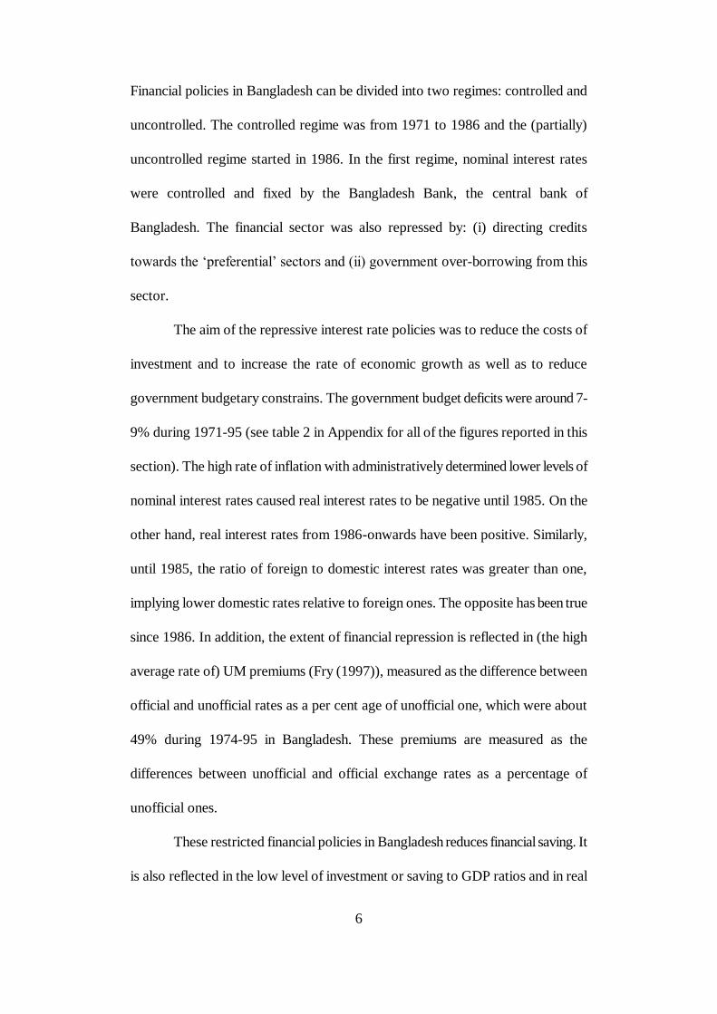
Financial policies in Bangladesh can be divided into two regimes: controlled and

uncontrolled. The controlled regime was from 1971 to 1986 and the (partially)

uncontrolled regime started in 1986. In the first regime, nominal interest rates

were controlled and fixed by the Bangladesh Bank, the central bank of

Bangladesh. The financial sector was also repressed by: (i) directing credits

towards the „preferential‟ sectors and (ii) government over-borrowing from this

sector.

The aim of the repressive interest rate policies was to reduce the costs of

investment and to increase the rate of economic growth as well as to reduce

government budgetary constrains. The government budget deficits were around 7-

9% during 1971-95 (see table 2 in Appendix for all of the figures reported in this

section). The high rate of inflation with administratively determined lower levels of

nominal interest rates caused real interest rates to be negative until 1985. On the

other hand, real interest rates from 1986-onwards have been positive. Similarly,

until 1985, the ratio of foreign to domestic interest rates was greater than one,

implying lower domestic rates relative to foreign ones. The opposite has been true

since 1986. In addition, the extent of financial repression is reflected in (the high

average rate of) UM premiums (Fry (1997)), measured as the difference between

official and unofficial rates as a per cent age of unofficial one, which were about

49% during 1974-95 in Bangladesh. These premiums are measured as the

differences between unofficial and official exchange rates as a percentage of

unofficial ones.

These restricted financial policies in Bangladesh reduces financial saving. It

is also reflected in the low level of investment or saving to GDP ratios and in real

7

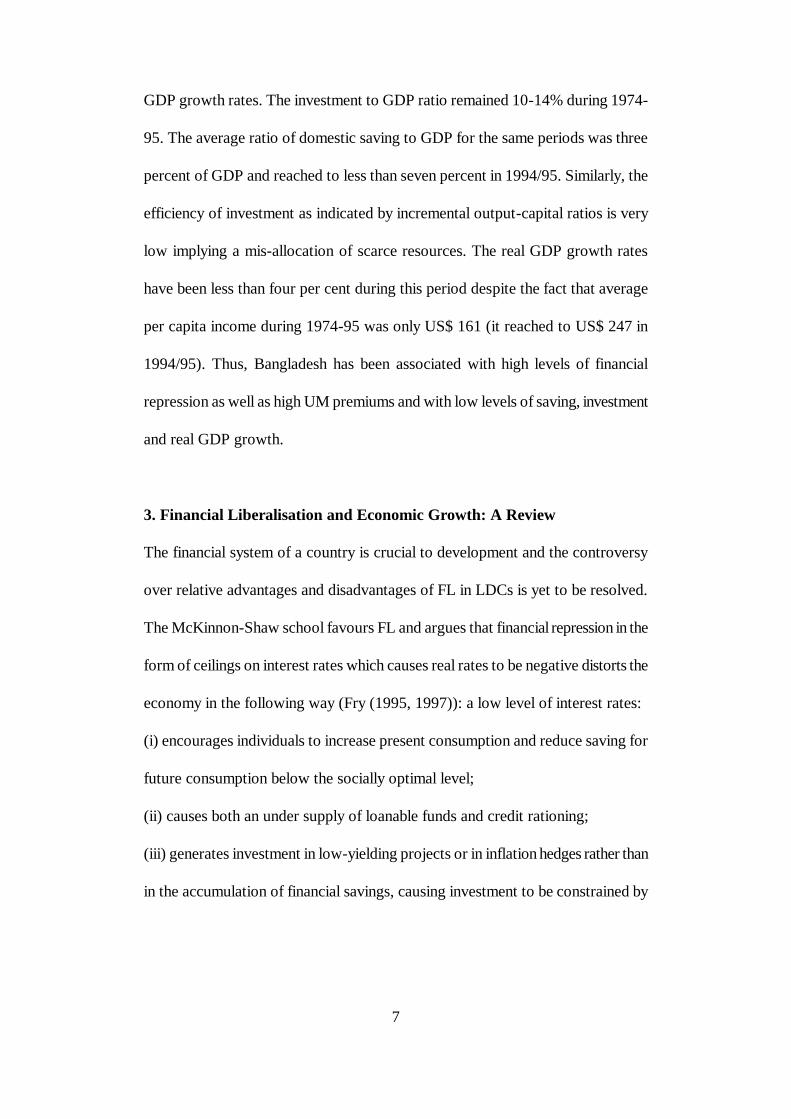
GDP growth rates. The investment to GDP ratio remained 10-14% during 1974-

95. The average ratio of domestic saving to GDP for the same periods was three

percent of GDP and reached to less than seven percent in 1994/95. Similarly, the

efficiency of investment as indicated by incremental output-capital ratios is very

low implying a mis-allocation of scarce resources. The real GDP growth rates

have been less than four per cent during this period despite the fact that average

per capita income during 1974-95 was only US$ 161 (it reached to US$ 247 in

1994/95). Thus, Bangladesh has been associated with high levels of financial

repression as well as high UM premiums and with low levels of saving, investment

and real GDP growth.

3. Financial Liberalisation and Economic Growth: A Review

The financial system of a country is crucial to development and the controversy

over relative advantages and disadvantages of FL in LDCs is yet to be resolved.

The McKinnon-Shaw school favours FL and argues that financial repression in the

form of ceilings on interest rates which causes real rates to be negative distorts the

economy in the following way (Fry (1995, 1997)): a low level of interest rates:

(i) encourages individuals to increase present consumption and reduce saving for

future consumption below the socially optimal level;

(ii) causes both an under supply of loanable funds and credit rationing;

(iii) generates investment in low-yielding projects or in inflation hedges rather than

in the accumulation of financial savings, causing investment to be constrained by

8

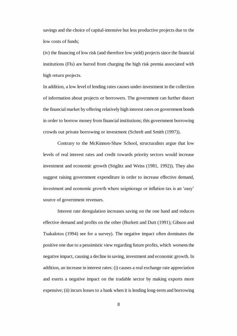
savings and the choice of capital-intensive but less productive projects due to the

low costs of funds;

(iv) the financing of low risk (and therefore low yield) projects since the financial

institutions (FIs) are barred from charging the high risk premia associated with

high return projects.

In addition, a low level of lending rates causes under-investment in the collection

of information about projects or borrowers. The government can further distort

the financial market by offering relatively high interest rates on government bonds

in order to borrow money from financial institutions; this government borrowing

crowds out private borrowing or investment (Schreft and Smith (1997)).

Contrary to the McKinnon-Shaw School, structuralists argue that low

levels of real interest rates and credit towards priority sectors would increase

investment and economic growth (Stiglitz and Weiss (1981, 1992)). They also

suggest raising government expenditure in order to increase effective demand,

investment and economic growth where seigniorage or inflation tax is an „easy‟

source of government revenues.

Interest rate deregulation increases saving on the one hand and reduces

effective demand and profits on the other (Burkett and Dutt (1991); Gibson and

Tsakalotos (1994) see for a survey). The negative impact often dominates the

positive one due to a pessimistic view regarding future profits, which worsens the

negative impact, causing a decline in saving, investment and economic growth. In

addition, an increase in interest rates: (i) causes a real exchange rate appreciation

and exerts a negative impact on the tradable sector by making exports more

expensive; (ii) incurs losses to a bank when it is lending long-term and borrowing

9

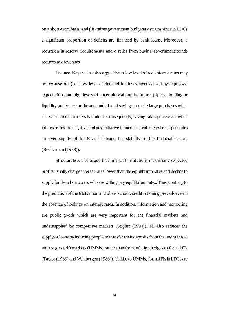
on a short-term basis; and (iii) raises government budgetary strains since in LDCs

a significant proportion of deficits are financed by bank loans. Moreover, a

reduction in reserve requirements and a relief from buying government bonds

reduces tax revenues.

The neo-Keynesians also argue that a low level of real interest rates may

be because of: (i) a low level of demand for investment caused by depressed

expectations and high levels of uncertainty about the future; (ii) cash holding or

liquidity preference or the accumulation of savings to make large purchases when

access to credit markets is limited. Consequently, saving takes place even when

interest rates are negative and any initiative to increase real interest rates generates

an over supply of funds and damage the stability of the financial sectors

(Beckerman (1988)).

Structuralists also argue that financial institutions maximising expected

profits usually charge interest rates lower than the equilibrium rates and decline to

supply funds to borrowers who are willing pay equilibrium rates. Thus, contrary to

the prediction of the McKinnon and Shaw school, credit rationing prevails even in

the absence of ceilings on interest rates. In addition, information and monitoring

are public goods which are very important for the financial markets and

undersupplied by competitive markets (Stiglitz (1994)). FL also reduces the

supply of loans by inducing people to transfer their deposits from the unorganised

money (or curb) markets (UMMs) rather than from inflation hedges to formal FIs

(Taylor (1983) and Wijnbergen (1983)). Unlike to UMMs, formal FIs in LDCs are

10

not user friendly and cannot lend on a one for one basis due to reserve

requirements.

A host of empirical studies have been carried out and the general findings

of them support the McKinnon and Shaw hypothesis, i.e. more liberalised financial

regimes are associated with faster economic growth (see Levin (197); Fry (1995);

Siddiki (1999a); Ghatak (1997)). However, most of the studies are based on

NGT. This dependence on NGT weakens the significance of positive relationships

between financial variables and economic growth, since the presence of

diminishing returns to capital as predicted by NGT dictates that long run growth

rates in per capita income will not be enhanced by an increase in the level of saving

and investment. This type of limitation of NGT motivates the emergence of

endogenous growth theory (EGT), which predicts that FL (King and Levine

(1993)) along with investment in physical (Romer (1986)) and human capital

(Lucas (1988)) enhance economic growth.

Using EGT, King and Levine predict that FIs increase the productivity of

investment and contribute economic growth by: efficiently evaluating projects and

selecting the most promising ones; pooling household savings and mobilising them

to finance more promising projects and sharing and diversifying risks associated

with innovations. FIs also contribute to the productivity of investment and

economic growth by reducing cash holding and liquid, i.e. unproductive,

investment to meet agents‟ future liquidity demand (Bencivenga and Smith

(1991)). In an another study, using cross-section data for 80 countries over the

period 1960-1989 and EGT, King and Levine (1993) show a significant positive

relationship between various financial indicators and real per capita income.

11

Roubini and Sala-i-Martin (1992) have also empirically shows that financial

repression causes high rates of inflation and a reduction in the productivity of

capital which in turn reduces economic growth rates.

4. The Theoretical Model

In this section, we extend the Pagano (1993) model to incorporate HC since FL

increases the quality of HC by financing education to financially constrained

households (Gregorio (1996)). EGT predicts that HC is one of the main engines of

economic growth - a common feature in LDCs. The Pagano model predicts that

FL increases: (i) saving and investment; (ii) the proportion of saving that goes to

investment and (iii) the efficiency of investment by improving competitiveness,

availability of information regarding the investment projects. Using an AK version

of endogenous growth model, Pagano postulates that these above three factors in

turn increase the rate of economic growth. Our extended model predicts that there

is an additional efficiency gain caused by the accumulation of HC resulting from

FL. To explain our model, assume that aggregate output is a linear function of the

aggregate capital stock:

where Yt is aggregate output, Kt is the aggregate capital stock and t is time. This

production function represents a competitive economy with the presence of

externality or spillover effects. Each firm faces constant returns to scale, but the

K A = Y tt

12

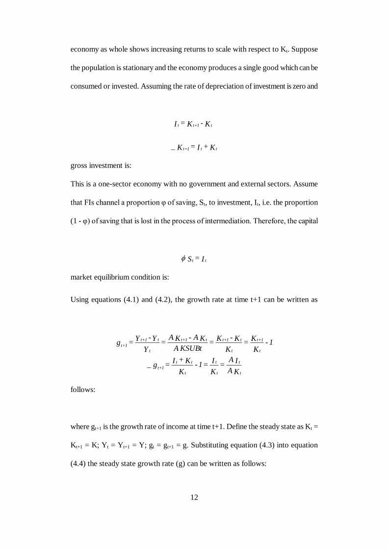
economy as whole shows increasing returns to scale with respect to Kt. Suppose

the population is stationary and the economy produces a single good which can be

consumed or invested. Assuming the rate of depreciation of investment is zero and

gross investment is:

This is a one-sector economy with no government and external sectors. Assume

that FIs channel a proportion φ of saving, St, to investment, It, i.e. the proportion

(1 - φ) of saving that is lost in the process of intermediation. Therefore, the capital

market equilibrium condition is:

Using equations (4.1) and (4.2), the growth rate at time t+1 can be written as

follows:

where gt+1 is the growth rate of income at time t+1. Define the steady state as Kt =

Kt+1 = K; Yt = Yt+1 = Y; gt = gt+1 = g. Substituting equation (4.3) into equation

(4.4) the steady state growth rate (g) can be written as follows:

K + I = K

K -K = I

tt1+t

t1+tt

_

I = S tt

K A

I A =

K

I = 1-

K

K + I = g

1 - K

K =

K

K-K =

KSUBt A

K A - K A =

Y

Y - Y =g

t

t

t

t

t

tt

1+t

t

1+t

t

t1+tt1+t

t

t1+t

1+t

_

13

where s is S/Y. Taking the logarithms of equation (4.5), we can write:

Equation 4.6 distinguishes three channels: φ, s and „A‟, through which FL could

influence economic growth. The transmission mechanisms are explained below.

4.1 Funnelling Saving to Investment

FIs collect private savings and direct them into investment. FIs cannot generally

transform all savings into investment since transaction costs and profits absorb

some of the funds. A proportion (1 - φ) of saving remains out of investment. FL in

the form of the expansion of bank branches and a reduction in reserve

requirements boosts competition among FIs, which reduces their commissions and

fees, the difference between lending and borrowing rates and hence there is a rise

in φ. The structural equation for φ can be written as follows:

where FDφt represents a vector of government financial policies which help or

hinder financial development and competition. The signs of the vector of

parameters φ1 are positive when policies reduce reserve requirements, restrictions

on new banks or branches and hence boost the financial markets, vice versa.

s A = Y

I A = g

s + + A = g lnlnlnln

u + FD + = tt10t lnln

14

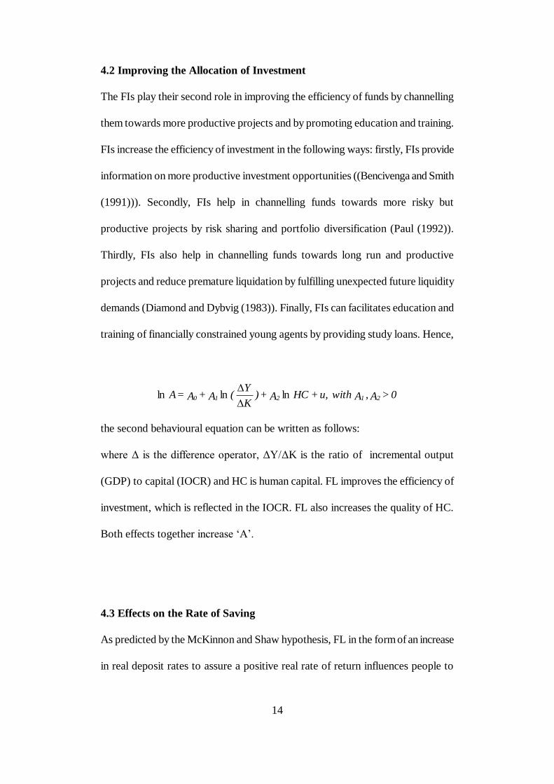
4.2 Improving the Allocation of Investment

The FIs play their second role in improving the efficiency of funds by channelling

them towards more productive projects and by promoting education and training.

FIs increase the efficiency of investment in the following ways: firstly, FIs provide

information on more productive investment opportunities ((Bencivenga and Smith

(1991))). Secondly, FIs help in channelling funds towards more risky but

productive projects by risk sharing and portfolio diversification (Paul (1992)).

Thirdly, FIs also help in channelling funds towards long run and productive

projects and reduce premature liquidation by fulfilling unexpected future liquidity

demands (Diamond and Dybvig (1983)). Finally, FIs can facilitates education and

training of financially constrained young agents by providing study loans. Hence,

the second behavioural equation can be written as follows:

where Δ is the difference operator, ΔY/ΔK is the ratio of incremental output

(GDP) to capital (IOCR) and HC is human capital. FL improves the efficiency of

investment, which is reflected in the IOCR. FL also increases the quality of HC.

Both effects together increase „A‟.

4.3 Effects on the Rate of Saving

As predicted by the McKinnon and Shaw hypothesis, FL in the form of an increase

in real deposit rates to assure a positive real rate of return influences people to

0> A ,A withu, +HC A + )K

Y( A + A = A 21210 lnlnln

15

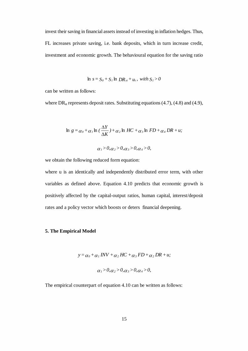
invest their saving in financial assets instead of investing in inflation hedges. Thus,

FL increases private saving, i.e. bank deposits, which in turn increase credit,

investment and economic growth. The behavioural equation for the saving ratio

can be written as follows:

where DRst represents deposit rates. Substituting equations (4.7), (4.8) and (4.9),

we obtain the following reduced form equation:

where u is an identically and independently distributed error term, with other

variables as defined above. Equation 4.10 predicts that economic growth is

positively affected by the capital-output ratios, human capital, interest/deposit

rates and a policy vector which boosts or deters financial deepening.

5. The Empirical Model

The empirical counterpart of equation 4.10 can be written as follows:

0 > S with,u + DR S + S = s 1tst10 lnln

0, > 0, > 0, > 0, >

u; + DR + FD + HC + )K

Y( + = g

4321

43210

lnlnlnln

0, > 0, > 0, > 0, >

u; + DR + FD + HC + INV + =y

4321

23210

16

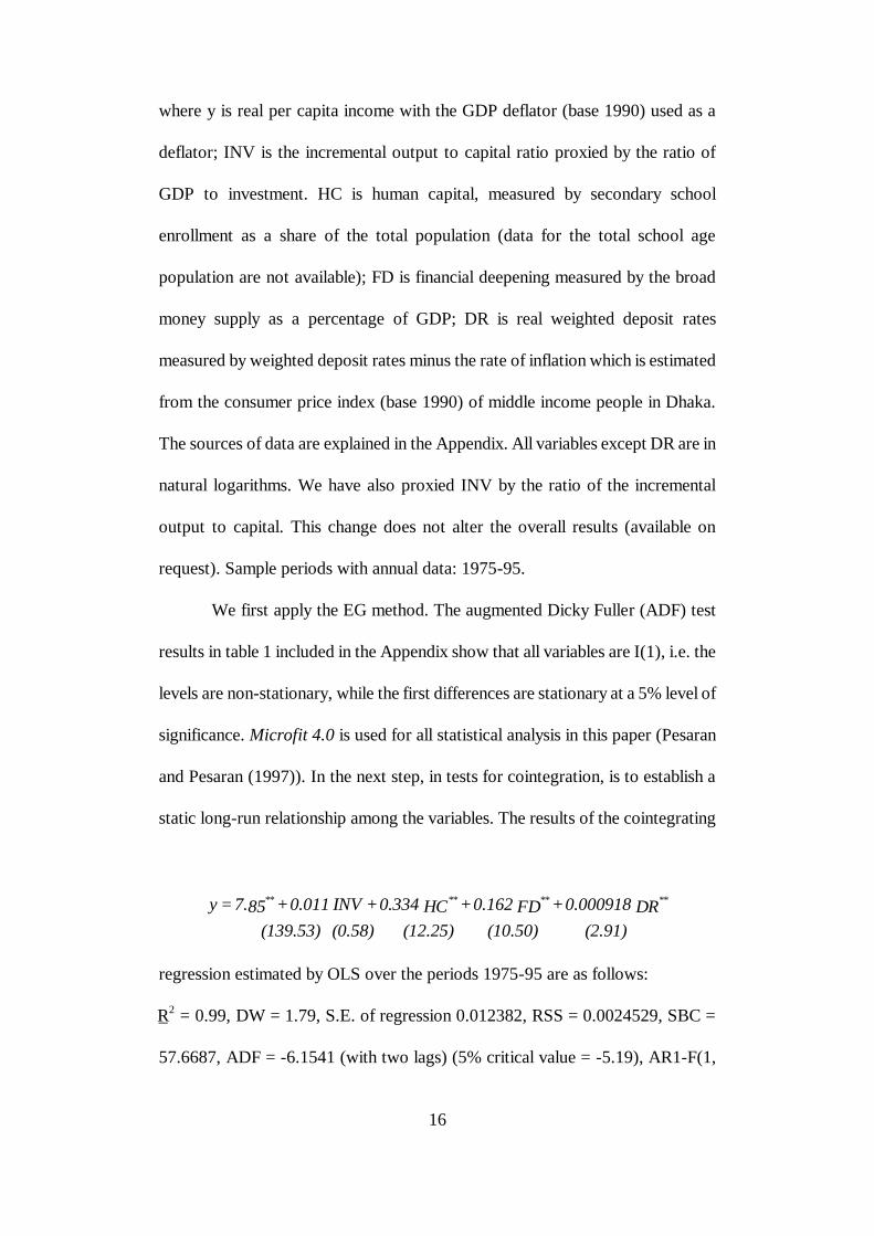
where y is real per capita income with the GDP deflator (base 1990) used as a

deflator; INV is the incremental output to capital ratio proxied by the ratio of

GDP to investment. HC is human capital, measured by secondary school

enrollment as a share of the total population (data for the total school age

population are not available); FD is financial deepening measured by the broad

money supply as a percentage of GDP; DR is real weighted deposit rates

measured by weighted deposit rates minus the rate of inflation which is estimated

from the consumer price index (base 1990) of middle income people in Dhaka.

The sources of data are explained in the Appendix. All variables except DR are in

natural logarithms. We have also proxied INV by the ratio of the incremental

output to capital. This change does not alter the overall results (available on

request). Sample periods with annual data: 1975-95.

We first apply the EG method. The augmented Dicky Fuller (ADF) test

results in table 1 included in the Appendix show that all variables are I(1), i.e. the

levels are non-stationary, while the first differences are stationary at a 5% level of

significance. Microfit 4.0 is used for all statistical analysis in this paper (Pesaran

and Pesaran (1997)). In the next step, in tests for cointegration, is to establish a

static long-run relationship among the variables. The results of the cointegrating

regression estimated by OLS over the periods 1975-95 are as follows:

_R2 = 0.99, DW = 1.79, S.E. of regression 0.012382, RSS = 0.0024529, SBC =

57.6687, ADF = -6.1541 (with two lags) (5% critical value = -5.19), AR1-F(1,

(2.91) (10.50) (12.25) (0.58) (139.53)

DR 0.000918+FD 0.162+HC 0.334+INV 0.011+857.=y ********

17

15) = 0.081378[0.779], AR1-λ2(1) = 0.11331[0.735], RESET-F(1,15) =

0.002928[0.958], RESET-λ2(1) = 0.0040994[0.949], NOR-λ

2(2) =

0.77[0.77686], H-λ2(1) = 3.1642[0.075], H-F(1, 19) = 3.3708[0.083], ARCH-

λ2(1) = 0.7654[0.395], ARCH- λ

2(2) = 2.1143[0.347].

Throughout our analysis, t-statistics are reported in the parentheses, **

and * represent 1% and 5% significance levels, respectively2. All the values are

statistically insignificant implying no evidence of mis-specification. Thus the model

(equation 5.2) passes all diagnostic tests. The variables are cointegrated at the 5%

level as the estimated ADF statistics are lower than the critical value. However,

the coefficient of INV is statistically insignificant in the both long- and the short-

run (see below). Excluding INV, we re-estimated the model as follows:

2

AR1-F and AR2-λ (2) are the F and chi square tests, respectively, for first order

residual joint autocorrelation; RESET-F and RESET-λ2 are the F and chi square

tests for mis-specified functional form; NOR-λ2(2) is the chi square statistic for

testing normality; H-λ2(1) and H-F are the chi square and F statistics, respectively,

for testing heteroscedasticity; ARCH-λ2(1) and ARCH-λ

2(2) are the first and

second order tests for autoregressive conditional heteroscedasticity; probability

values are reported in the square brackets.

_R2 = 0.99, DW = 1.81, S.E. of regression 0.01236, RSS = 0.0025038, SBC =

58.9752, ADF = -5.8155 (with two lags) (5% critical value = -4.7635), AR1-F(1,

16) = 0.056836[0.815], AR1-λ2(1) = 0.074[0.785], RESET-F(1,16) =

(3.19) (10.70) (12.60) (258.195)

DR 0.000815 + FD 0.161 + HC 0.331 + 887. =y ********

18

0.025[0.877], RESET-λ2(1) = 0.03[0.858], NOR-λ

2(2) = 1.075[0.584], H-λ

2(1) =

3.79[0.052], H-F(1, 19) = 4.18[0.055], ARCH- λ2(1) = 0.70142[0.402], ARCH-

λ2(2) = 0.553[0.468].

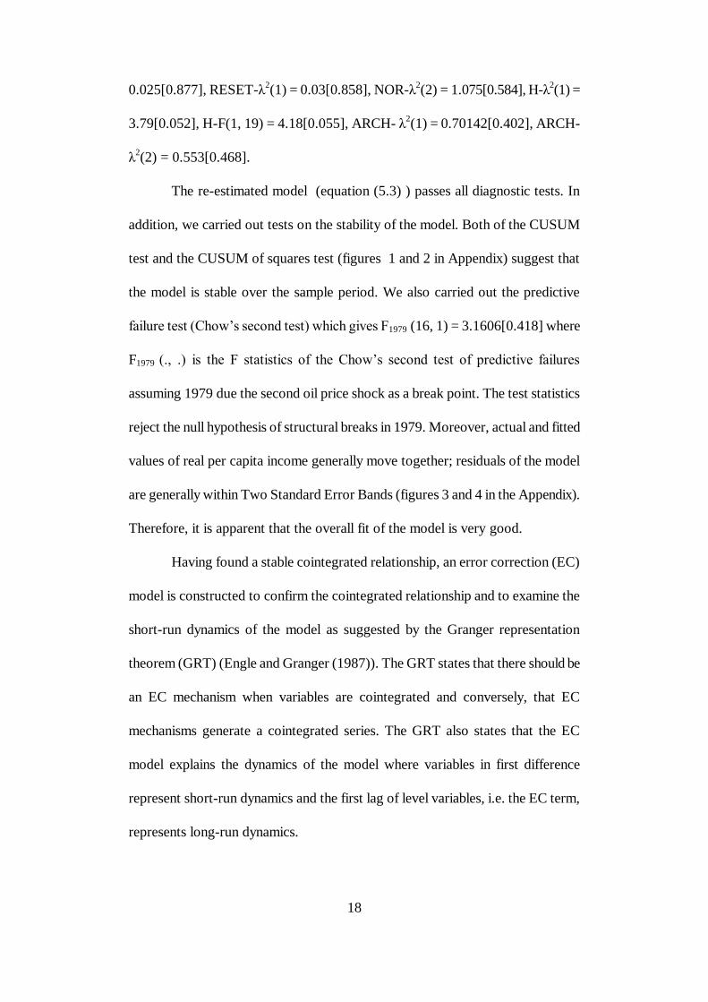
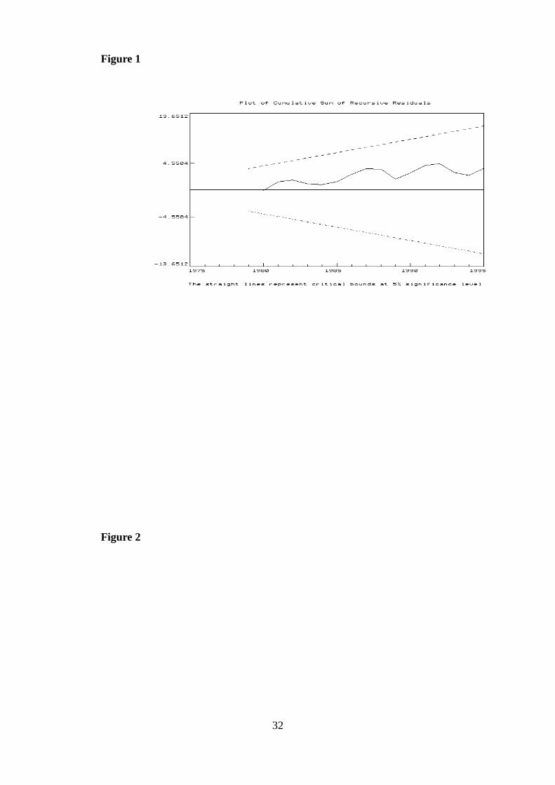
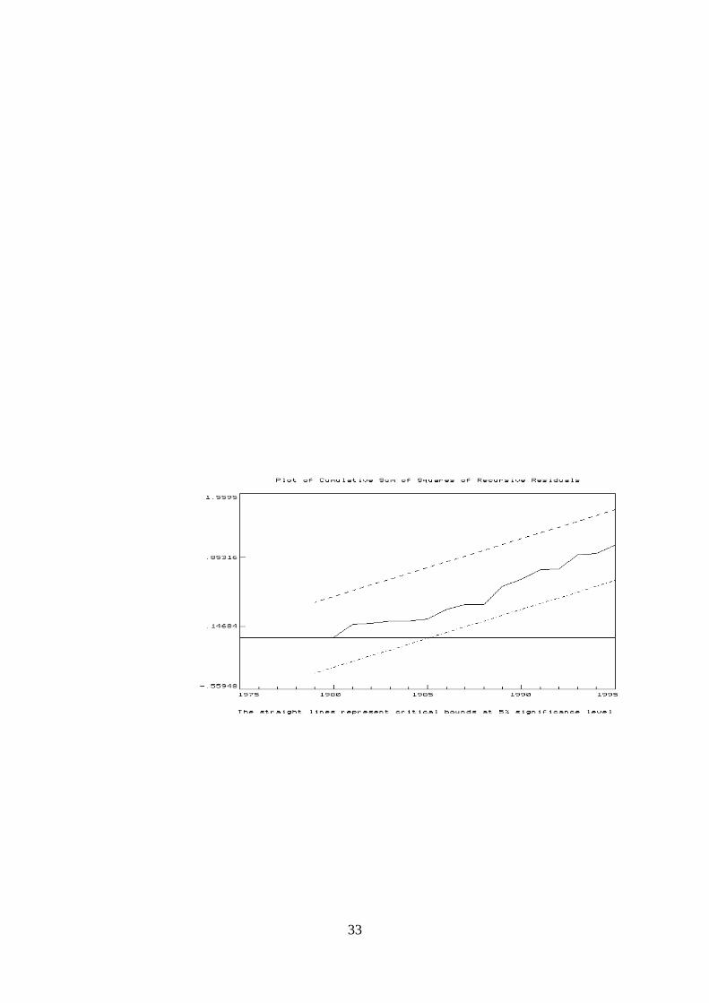
The re-estimated model (equation (5.3) ) passes all diagnostic tests. In

addition, we carried out tests on the stability of the model. Both of the CUSUM

test and the CUSUM of squares test (figures 1 and 2 in Appendix) suggest that

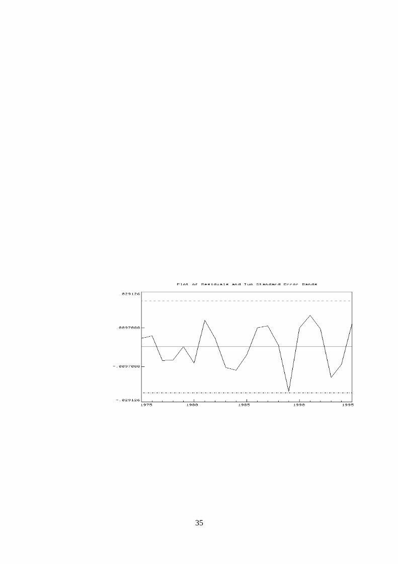
the model is stable over the sample period. We also carried out the predictive

failure test (Chow‟s second test) which gives F1979 (16, 1) = 3.1606[0.418] where

F1979 (., .) is the F statistics of the Chow‟s second test of predictive failures

assuming 1979 due the second oil price shock as a break point. The test statistics

reject the null hypothesis of structural breaks in 1979. Moreover, actual and fitted

values of real per capita income generally move together; residuals of the model

are generally within Two Standard Error Bands (figures 3 and 4 in the Appendix).

Therefore, it is apparent that the overall fit of the model is very good.

Having found a stable cointegrated relationship, an error correction (EC)

model is constructed to confirm the cointegrated relationship and to examine the

short-run dynamics of the model as suggested by the Granger representation

theorem (GRT) (Engle and Granger (1987)). The GRT states that there should be

an EC mechanism when variables are cointegrated and conversely, that EC

mechanisms generate a cointegrated series. The GRT also states that the EC

model explains the dynamics of the model where variables in first difference

represent short-run dynamics and the first lag of level variables, i.e. the EC term,

represents long-run dynamics.

19

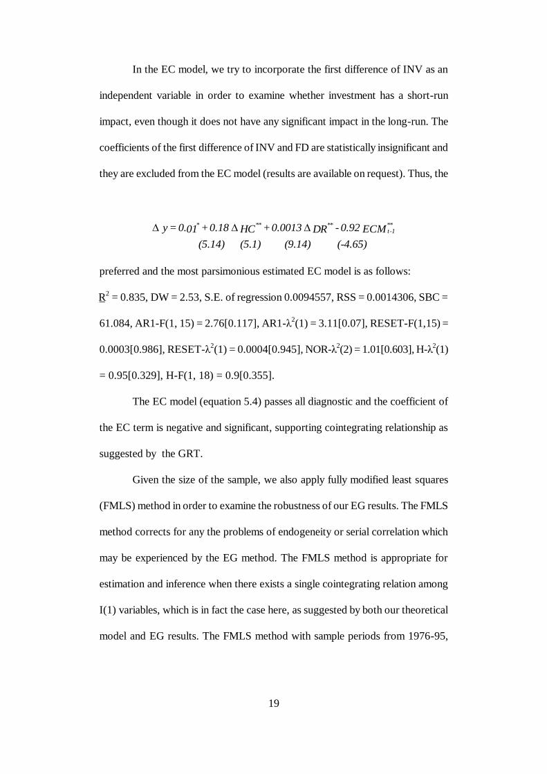
In the EC model, we try to incorporate the first difference of INV as an

independent variable in order to examine whether investment has a short-run

impact, even though it does not have any significant impact in the long-run. The

coefficients of the first difference of INV and FD are statistically insignificant and

they are excluded from the EC model (results are available on request). Thus, the

preferred and the most parsimonious estimated EC model is as follows:

_R2 = 0.835, DW = 2.53, S.E. of regression 0.0094557, RSS = 0.0014306, SBC =

61.084, AR1-F(1, 15) = 2.76[0.117], AR1-λ2(1) = 3.11[0.07], RESET-F(1,15) =

0.0003[0.986], RESET-λ2(1) = 0.0004[0.945], NOR-λ

2(2) = 1.01[0.603], H-λ

2(1)

= 0.95[0.329], H-F(1, 18) = 0.9[0.355].

The EC model (equation 5.4) passes all diagnostic and the coefficient of

the EC term is negative and significant, supporting cointegrating relationship as

suggested by the GRT.

Given the size of the sample, we also apply fully modified least squares

(FMLS) method in order to examine the robustness of our EG results. The FMLS

method corrects for any the problems of endogeneity or serial correlation which

may be experienced by the EG method. The FMLS method is appropriate for

estimation and inference when there exists a single cointegrating relation among

I(1) variables, which is in fact the case here, as suggested by both our theoretical

model and EG results. The FMLS method with sample periods from 1976-95,

(-4.65) (9.14) (5.1) (5.14)

ECM 0.92 - DR 0.0013 + HC 0.18 + 010. =y **1-t

*****

20

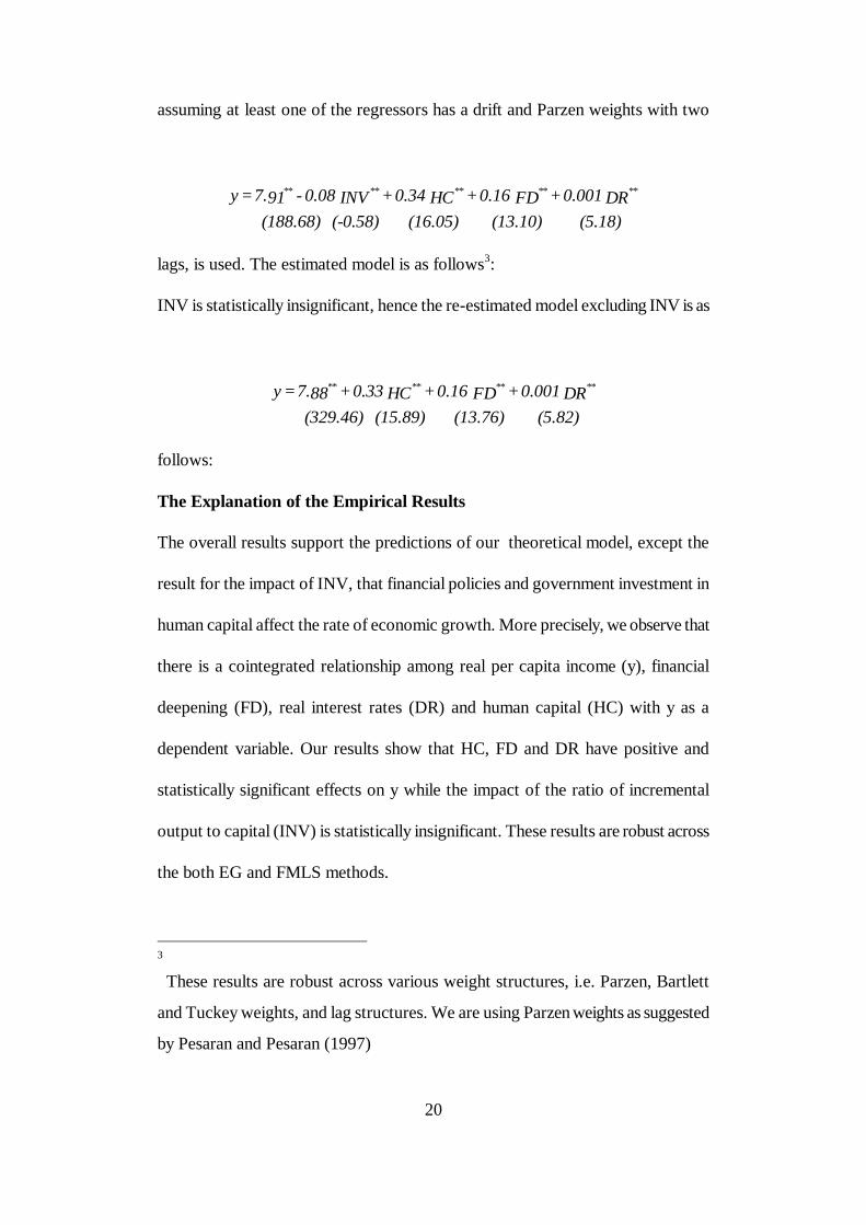
assuming at least one of the regressors has a drift and Parzen weights with two

lags, is used. The estimated model is as follows3:

INV is statistically insignificant, hence the re-estimated model excluding INV is as

follows:

The Explanation of the Empirical Results

3

These results are robust across various weight structures, i.e. Parzen, Bartlett

and Tuckey weights, and lag structures. We are using Parzen weights as suggested

by Pesaran and Pesaran (1997)

The overall results support the predictions of our theoretical model, except the

result for the impact of INV, that financial policies and government investment in

human capital affect the rate of economic growth. More precisely, we observe that

there is a cointegrated relationship among real per capita income (y), financial

deepening (FD), real interest rates (DR) and human capital (HC) with y as a

dependent variable. Our results show that HC, FD and DR have positive and

statistically significant effects on y while the impact of the ratio of incremental

output to capital (INV) is statistically insignificant. These results are robust across

the both EG and FMLS methods.

(5.18) (13.10) (16.05) (-0.58) (188.68)

DR 0.001 +FD 0.16 +HC 0.34 +INV 0.08 - 917. =y **********

(5.82) (13.76) (15.89) (329.46)

DR 0.001 + FD 0.16 + HC 0.33 + 887. =y ********

21

The overall results reveal the highest positive real per capita income

elasticity with respect to investment in HC. These results support the prediction of

EGT which suggests that the improvement of the quality of working population is

very important in the development process. Importantly, investment in education

increases knowledge which in turn has effects on other sectors. Note also that R &

D, innovation, specialisation and high technology projects require skilled

manpower and these are unachievable in the absence of investment in HC.

We also observe that the impact of INV on y is statistically insignificant.

This result is not unexpected since it is widely accepted that the quality of both

government and private physical investment in Bangladesh is very low because of

prevalent corruption and bureaucratic red tape associated with both government

investment and loans for private sector investment (Ahmed et al. (1991); Hossain

and Rashid, (1997)). There is, for example, a very common practice in Bangladesh

of grasping depositors‟ money from banks using bribes, personal influences and

political pressures, making „false‟ investment and then declaring the business as

„sick‟. The essence of the result on investment is that the quality in addition to the

quantity of investment is important in order to increase economic growth.

Our results also show that FD has a statistically significant and positive

impact on y, which is consistent with our theoretical model that an increase in FD

raises the supply or the availability of funds which in turn increases investment

and economic growth. However, the magnitude of this effect is not very high. The

low effectiveness of FD and the statistically insignificant impact of INV highlight

the inefficiency of the government sector and the poor management of credit that

22

goes to the private sector ((Ahmed et al. (1991); Hossain and Rashid, (1997)). In

the case of Bangladesh, until the early 1990s, a significant proportion of credit was

taken by the government to finance budget deficits. Credit to the private sector

was confined to some selective borrowers who were politically and socially very

influential. Thus, low FD implies that the banking sector serves only the

government and influential borrowers and hence, productive potential borrowers

were left with no credit. On the other hand, an increase in FD implies that FIs have

more ability to lend potential borrowers.

The empirical results also support the prediction that DR positively affect

y. The main policy consideration of the McKinnon and Shaw hypothesis is to

increase DR to a positive level to encourage financial saving. A real positive or

market clearing DR encourages borrowers to undertake only those projects which

have returns above market clearing interest rates. Market clearing interest rates

also reduce inefficiency associated with directed loans towards preferential

sectors. Our results support these views. However, the magnitude of the

coefficient of real rates is very low which is consistent with other findings on

developing countries (Ghatak (1995)). This low interest elasticity is mainly due to

the low level of y in Bangladesh. Since most of the earnings of people are spent on

basic needs, people are left with very little money to save. The very small but

significant coefficient of DR implies that DR liberalisation alone is unlikely to be

able to expedite economic growth in Bangladesh.

Note that the impact of FD on y is much higher than that of DR. An

increase in FD is tantamount to a rise in the capacity for financial intermediation.

On the other hand, an increase in DR indicates a rise in the costs of borrowing.

23

Thus, our results support the view that the availability of credit rather than their

opportunity costs is the more important determinant of y in a LDC like

Bangladesh.

To sum up, our long-run results show that HC, FD and DR have

statistically significant and positive impact on y, though the magnitude of the

impact of DR is small. On the other hand, the impact of INV is statistically

insignificant, implying that quality of investment is also important to increase y.

Finally, the coefficients of ΔHC and ΔDR in our EC model are statistically

significant and positive, implying that short-run dynamics of these variables are

also effective (equation 5.4). That is, y rises in the short-run in response to

increases in HC and DR. In the short-run, INV and FD does not have any

statistically significant impact on y. The short-run insignificant impact of FD may

be due to the fact that there is a time delay in the transfer of available funds from

the financial system to investment.

24

6. Conclusions

In this paper, we have developed an endogenous growth model including the ratio

of incremental output to capital (INV), investment in human capital (HC),

financial deepening (FD) and real interest rates (DR). This model predicts that

economic growth mainly is generated from three factors: the proportion of saving

channelled to investment (φ); (ii) the marginal productivity of capital (A) and (iii)

the ratios of saving GDP (s). Financial liberalisation (FL) in the form of interest

rate deregulation and an increase in FIs or financial deepening influences economic

growth by raising φ, A and s.

Our model predicts that a rise in real interest rates raises the returns on

financial saving and encourages people to divert funds from non-financial to

financial assets, i.e. an increase in s. An increase in FIs also raises competition and

reduces investment leakage and thus a rise in φ. FIs increase the efficiency of

investment by: (a) collecting information on investment opportunities; (b)

providing the scope of risk sharing through portfolio diversification; (c) promoting

training and education.

This model has been applied to Bangladesh using annual data from 1975-

95, cointegration analysis and the fully modified least squares (FMLS) method.

The results are robust across both methodologies. Our results reveal that there is

multivariate cointegrated relationship among y, HC, FD and DR where y is the

dependent variable, supporting the view that FD, DR and HC are important

factors in boosting economic growth.

The results reveal that HC is the one of the most important factors for

increasing the growth of y. These results highlight the fact that development in

25

Bangladesh crucially depends on investment in education. The impact of INV on y

is statistically insignificant. The insignificant impact of INV is not unexpected due

to prevalent corruption associated with both government investment and the

allocation of credit for private investment.

We also observe that FD has a significant positive impact on the growth of

y, which is in accord with our theoretical model. FL reduces direct lending and

borrowing and increases FD and the availability of funds. FIs also channel funds

towards efficient projects. Thus, an increase in FD increases the supply of

investment towards relatively more productive sectors and hence, generates the

growth of y. In addition, a rise in DR increases the supply of loanable funds as

people are encouraged to hold financial assets instead of investing in inflation

hedges and thus a rise in economic growth.

However, the magnitude of the coefficient of DR is very low because of

very low level of y and distortions in the financial sector. The very small but

significant coefficient of DR also implies that the deregulation of interest rates

alone are unlikely to be able to expedite economic growth in Bangladesh. The

greater impact of FD than of DR implies that the availability rather than the

opportunity costs (DR) of funds is more important in stimulating economic

growth in Bangladesh.

26

References

Ahmed, B. et al. (1991), Government Malpractices, in Managing the

Development Process (Volume two) Report of the Task Forces on Bangladesh

Development Strategies for the 1990's.

Ahmed, S. M. and Ansari, M. (1995) Financial Development In Bangladesh - A

test of McKinnon-Shaw Hypothesis, Canadian Journal of Development Studies,

Vol. XVI(2), p. 291-302.

Beckerman, P. (1988) The Consequences of “Upward Financial Repression”,

International Review of Applied Economics, 2(1), 233-49.

Bencivenga, Valerie R. and Smith, Bruce D. (1991) Financial Intermediation and

Endogenous Growth, Review of Economic Studies, 58, 195-209.

Burkett, P. and Dutt, A.K. (1991) Interest Rate Policy, Effective Demand and

Growth in LDCs, International Review of Applied Economics, 5(2), 127-54.

Diamond, Douglas W. and Dybvig, Philip H. (1983) Bank Runs, Deposit

Insurance and Liquidity, Journal of Political Economy, 91(3), 401-19.

Engle, R. F. and Granger, C. W. J. (1987) Cointegration and Error Correction:

Representation, Estimation and Testing, Econometrica, 52, 251-76.

Fry, Maxwell J. (1995) Money Interest, and Banking in Economic Development,

Second Edition, The Johns Hopkins University Press, London.

Fry, Maxwell J. (1997) In Favour of Financial Development, The Economic

Journal, 107, 754-77.

Ghatak, S. (1995) Monetary Economics in Developing Countries, Second

Edition, Mcmillan Press Limited, UK.

27

Ghatak, S. (1997) Financial Liberalisation: The Case of Sri Lanka, Empirical

Economics, 22 (1), 117-31.

Gregorio, José de (1996) Borrowing Constraints, Constraints, Human Capital

Accumulation, and Growth, Journal of Monetary Economics, 37, p. 49-71.

Hossain, A. and Rashid, S. (1997) Financial Sector Reform, in (ed.) Quibria, M.G.

The Bangladesh Economy in Transition, Oxford University Press and Asian

Development Bank.

Jappeli, Tullio and Pagano, Marco (1994) Savings, Growth and Liquidity

Constraints, Quarterly Journal of Economics, 109(1), 83-109.

King, Robert G. and Levine, R. (1993) Finance, Entrepreneurship, and Growth:

Theory and Evidence, Journal of Monetary Economics, 32(3), 513-42.

Levine, R. (1997) Financial Development and Economic Growth: Views and

Agenda, Journal of Economic Literature, XXXV, p. 688-726.

Lucas, R. E. (1988) On the Mechanism of Economic Development, Journal of

Monetary Economics, 22, 3-42.

McKinnon, Ronald (1973) Money and Capital in Economic Development, The

Brooking Institution, Washington, D.C.

Pagano, M (1993). Financial Markets and Growth: An Overview, European

Economic Review, 37, 613-22.

Pesaran, M. H. and Pesaran, B. (1997) Microfit 4.0, Oxford University Press,

Oxford.

28

Phillips. C.B. and Hansen, B. E. (1990) Statistical Inference in the Instrumental

Variables Regression with I(1) Processes, Review of Economic Studies, 57, 99-

125.

Romer, P. M. (1986) Increasing Returns and Long-run Growth, Journal of

Political Economy, Vol. 94, p. 1002-1037.

Roubini, Nouriel and Sala-i-Martin, Xavier (1992) Financial Repression and

Economic Growth, Journal of Development Economics, 39, 5-30.

Saint-Paul, G., (1992) Technological Choice, Financial Markets and Economic

Development, European Economic Review, 36, 763-81.

Schreft, Stacey L. and Smith, Bruce D. (1997) Money, Banking, and Capital

Formation, Journal of Economic Theory, 73, 157-82.

Shaw, E. (1973) Financial Deepening in Economic Development, Oxford

University Press.

Siddiki, J. U. (1999a) Economic Liberalisation and Growth in Bangladesh: 1974-

95, PhD Thesis, Kingston University, England.

Siddiki, J. U. (1999b) Demand for Money in Bangladesh: A Cointegration

Analysis, Applied Economics, Forthcoming.

Stiglitz, Joseph E. (1994) The Role of the State in Financial Markets, In

Proceedings of the World Bank Conference on Development Economics, (eds)

Michael Bruno and Boris Pleskovic, World Bank, Washington, D. C..

Stiglitz, Joseph E. and Weiss, A. (1981) Credit Rationing in Markets with

Imperfect Information, American Economic Review, 71(3), 393-410.

29

Stiglitz, Joseph E. and Weiss, A. (1992) Asymmetric Information in Credit

Markets and Its Implication for Macro-Economics, Oxford Economic Papers, 44,

694-724.

Taylor, L. (1983) Structuralist Macroeconomics: Applicable Models in the Third

World, Basic Books, New York.

van Wijnbergen, Sweder (1983a) Interest Rate Management in LDC‟s, Journal of

Monetary Economics, 12, 433-52.

30

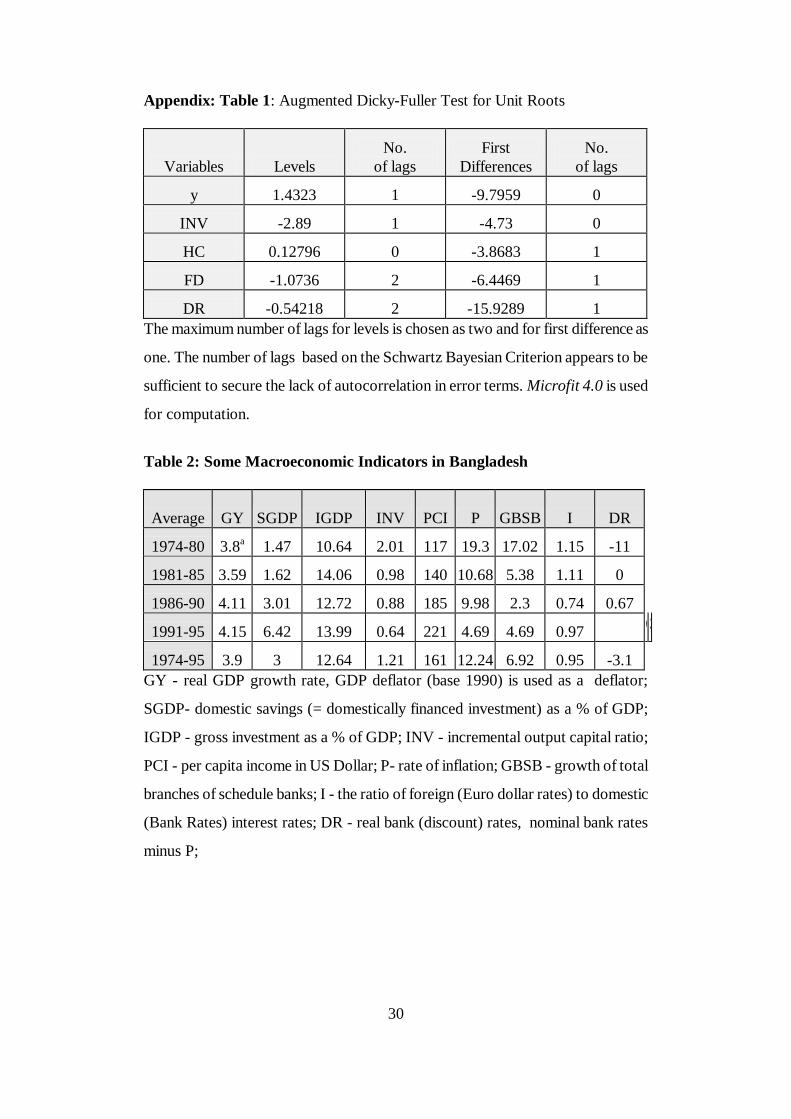
Appendix: Table 1: Augmented Dicky-Fuller Test for Unit Roots

Variables Levels

No.

of lags

First

Differences

No.

of lags

y 1.4323 1 -9.7959 0

INV -2.89 1 -4.73 0

HC 0.12796 0 -3.8683 1

FD -1.0736 2 -6.4469 1

DR -0.54218 2 -15.9289 1

The maximum number of lags for levels is chosen as two and for first difference as

one. The number of lags based on the Schwartz Bayesian Criterion appears to be

sufficient to secure the lack of autocorrelation in error terms. Microfit 4.0 is used

for computation.

Table 2: Some Macroeconomic Indicators in Bangladesh

GRM2 GRM290

17.7 33.16

26.98 42.09

16.18 24.3

13.63 18.01

18.58 29.57

Average GY SGDP IGDP INV PCI P GBSB I DR

1974-80 3.8a 1.47 10.64 2.01 117 19.3 17.02 1.15 -11

1981-85 3.59 1.62 14.06 0.98 140 10.68 5.38 1.11 0

1986-90 4.11 3.01 12.72 0.88 185 9.98 2.3 0.74 0.67

1991-95 4.15 6.42 13.99 0.64 221 4.69 4.69 0.97 0

.

7

3

.

8

7

1974-95 3.9 3 12.64 1.21 161 12.24 6.92 0.95 -3.1

GY - real GDP growth rate, GDP deflator (base 1990) is used as a deflator;

SGDP- domestic savings (= domestically financed investment) as a % of GDP;

IGDP - gross investment as a % of GDP; INV - incremental output capital ratio;

PCI - per capita income in US Dollar; P- rate of inflation; GBSB - growth of total

branches of schedule banks; I - the ratio of foreign (Euro dollar rates) to domestic

(Bank Rates) interest rates; DR - real bank (discount) rates, nominal bank rates

minus P;

31

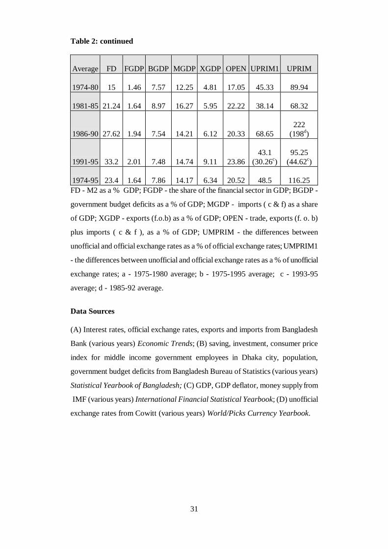
Table 2: continued

Average FD FGDP BGDP MGDP XGDP OPEN UPRIM1 UPRIM

1974-80 15 1.46 7.57 12.25 4.81 17.05 45.33 89.94

1981-85 21.24 1.64 8.97 16.27 5.95 22.22 38.14 68.32

1986-90 27.62 1.94 7.54 14.21 6.12 20.33 68.65

222

(198d)

1991-95 33.2 2.01 7.48 14.74 9.11 23.86

43.1

(30.26c)

95.25

(44.62c)

1974-95 23.4 1.64 7.86 14.17 6.34 20.52 48.5 116.25

FD - M2 as a % GDP; FGDP - the share of the financial sector in GDP; BGDP -

government budget deficits as a % of GDP; MGDP - imports ( c & f) as a share

of GDP; XGDP - exports (f.o.b) as a % of GDP; OPEN - trade, exports (f. o. b)

plus imports ( c & f ), as a % of GDP; UMPRIM - the differences between

unofficial and official exchange rates as a % of official exchange rates; UMPRIM1

- the differences between unofficial and official exchange rates as a % of unofficial

exchange rates; a - 1975-1980 average; b - 1975-1995 average; c - 1993-95

average; d - 1985-92 average.

Data Sources

(A) Interest rates, official exchange rates, exports and imports from Bangladesh

Bank (various years) Economic Trends; (B) saving, investment, consumer price

index for middle income government employees in Dhaka city, population,

government budget deficits from Bangladesh Bureau of Statistics (various years)

Statistical Yearbook of Bangladesh; (C) GDP, GDP deflator, money supply from

IMF (various years) International Financial Statistical Yearbook; (D) unofficial

exchange rates from Cowitt (various years) World/Picks Currency Yearbook.

32

Figure 1

Figure 2

33

34

Figure 3

Figure 4

35