i

FINANCIAL INTEGRATION, TRADE INTEGRATION,

MACROECONOMIC VOLATILITY AND ECONOMIC GROWTH

IN THE EAST AFRICAN COMMUNITY

BY

ONESMUS MUTUNGA NZIOKA

A RESEARCH THESIS SUBMITTED TO THE SCHOOL OF BUSINESS IN

PARTIAL FULFILLMENT OF THE REQUIREMENTS FOR THE AWARD

OF THE DEGREE OF DOCTOR OF PHILOSOPHY IN BUSINESS

ADMINISTRATION OF THE UNIVERSITY OF NAIROBI

2017

ii

DECLARATION

This thesis report is my original work and has not been presented for a degree in any

other University.

Signature…………………………………………. Date………………………

Onesmus Mutunga Nzioka

D80/61474/2011

This thesis report has been submitted for examination with our approval as the University

Supervisors.

Signature………………………………….. Date…………………….

Professor. Erasmus Kaijage,

Professor, Department of Finance and Accounting,

School of Business, University of Nairobi.

Signature……………...................................... Date……………………

Professor. Josiah Aduda,

Professor, Department of Finance and Accounting,

School of Business, University of Nairobi.

Signature……………...................................... Date……………………

Dr. Duncan Elly Ochieng

Lecturer, Department of Finance and Accounting

School of Business, University of Nairobi.

iii

ACKNOWLEDGEMENT

Firstly, I thank God almighty who has brought me this far and providing me with

strength, wisdom and vitality that has helped me to make this research work a reality.

Secondly, I would wish to thank my family for moral support, encouragement and their

understanding when I was not there for them during the project period; i wouldn‘t have

made it this far without them.

Special mention goes to my supervisors; Professor. Kaijage, Professor. Aduda and Dr.

Elly for their consistent guidance in transforming my raw initial thoughts at the proposal

stage to a full thesis report. The intellectual input by Professor Phokharyal, Dr. Okwiri

and Dr. Vincent Machuki cannot be taken for granted for the significant impact it made in

producing a quality document. The critical and dynamic views presented by various

discussants (Dr. Iraki, Dr. Sifunjo, Dr. Iraya, Dr. Mirie and Dr. Yabs) at the three stages

of the research proposal, provided the necessary and sufficient completeness and

accuracy required of any doctoral research work.

I also acknowledge the contribution of the University of Nairobi management, for the

provision of the necessary financial resources and information services courtesy of the

office of the deputy vice chancellor, Finance and administration as well as the PhD

library assistants; Regina and Mrs Noreh. The invaluable technical support by Thomas

Muthama during the research process can equally, not be ignored. Colleagues, comrades

and friends in deed, I salute you. God bless you all.

iv

DEDICATION

I dedicate this thesis to my dear family members who serve as the second pillar of my

life, after my creator for providing me with the perfect opportunity and the necessary

inspiration to pursue my studies in a seamless manner. It is this opportunity that has laid a

firm foundation to my academic journey and the fearless pursuit of my purpose in life.

v

TABLE OF CONTENTS

DECLARATION .................................................................................................................ii

ACKNOWLEDGEMENT ..................................................................................................iii

DEDICATION .....................................................................................................................iv

LIST OF FIGURES ............................................................................................................xi

LIST OF ABBREVIATIONS ............................................................................................xii

ABSTRACT ..........................................................................................................................xiv

CHAPTER ONE: INTRODUCTION ...............................................................................1

1.1 Background to the Study .................................................................................................1

1.1.1 Financial Integration ........................................................................................3

1.1.2 Economic Growth ............................................................................................5

1.1.3 Macroeconomic Volatility ................................................................................7

1.1.4 Trade Integration ..............................................................................................8

1.1.5 Benefits of Financial Integration .....................................................................10

1.1.5.1 Risk Sharing ..................................................................................................11

1.1.5.2 Improved Capital Allocation .........................................................................12

1.1.5.3 Economic Growth .........................................................................................13

1.1.5.4 Financial development ..................................................................................14

1.1.6 Expected Relationships ....................................................................................15

1.1.7 The East African Community ..........................................................................16

1.2 Research Problem ...........................................................................................................19

1.3 Research Questions .........................................................................................................22

1.4 Research Objectives ........................................................................................................22

vi

1.5 Value of the Study ..........................................................................................................23

1.6 Organization of the Thesis ..............................................................................................24

CHAPTER TWO: LITERATURE REVIEW ..................................................................26

2.1 Introduction .....................................................................................................................26

2.2 Theoretical Review .........................................................................................................26

2.2.1 Optimum Currency Area Theory .....................................................................26

2.2.2 New Economic Integration Theory ..................................................................30

2.2.3 Purchasing Power Parity (PPP) Theory ...........................................................33

2.2.4 Hegemonic Stability Theory ............................................................................35

2.2.5 Customs Unions Theory ..................................................................................37

2.3 Measuring Financial Integration .....................................................................................41

2.4 Empirical Literature Review ...........................................................................................46

2.4.1 Extent of Financial Integration ........................................................................46

2.4.3 Financial Integration and Economic Growth ...................................................48

2.4.4 Financial Integration and Macroeconomic Volatility ......................................52

2.4.2 Macro-economic Volatility and Economic Growth .........................................54

2.4.5 Macroeconomic Volatility and Trade Integration ............................................56

2.4.6 Financial Integration, Macroeconomic Volatility and Economic Growth .......58

2.5 Summary of Literature Review and Research Gaps .......................................................60

2.6 The Conceptual Framework ............................................................................................69

2.7 Research Hypotheses ......................................................................................................72

CHAPTER THREE: RESEARCH METHODOLOGY .................................................73

3.1 Introduction .....................................................................................................................73

vii

3.2 Research Philosophy .......................................................................................................73

3.3 Research Design ..............................................................................................................75

3.4 Population of the Study ...................................................................................................77

3.5 Operationalization of the Variables ................................................................................77

3.6 Data Collection ...............................................................................................................79

3.7 Data Analysis and Diagnostic Tests ...............................................................................80

3.8 Assumptions of the Study ................................................................................................83

3.9 Ethical Considerations ....................................................................................................83

CHAPTER FOUR: DATA DESCRIPTION AND ANALYSIS .....................................85

4.1 Introduction .....................................................................................................................85

4.2 Descriptive Statistics for the EAC Member states ..........................................................85

4.2.1 Descriptive Statistics for Burundi ....................................................................86

4.2.2 Descriptive Statistics for Kenya .......................................................................88

4.2.3 Descriptive Statistics for Rwanda .....................................................................92

4.2.4 Descriptive Statistics for Tanzania ................................................................... 96

4.2.5 Descriptive Statistics for Uganda .....................................................................101

4.2.6 Comparative Observations on the Descriptive statistics ..................................105

4.3 Multicollinearity Test ......................................................................................................107

4.4 Correlation Analysis .......................................................................................................109

4.4.1 Economic Growth and Financial Integration ...................................................109

4.4.2 Economic Growth and Macro-economic Volatility .........................................109

4.4.3 Financial Integration and Financial Deepening ...............................................110

4.4.4 Financial Integration and Trade Integration ....................................................110

viii

4.4.5 Financial Integration and Macro-economic Volatility .....................................110

4.4.6 Trade Integration and Macro-Economic Volatility ..........................................111

4.5 Unit Root Tests ...............................................................................................................112

4.6 Rationalizing the choice of model ..................................................................................114

4.6.1 Hausman Test for fixed effects and random effects models ............................116

4.7 Chapter summary ...........................................................................................................116

CHAPTER FIVE: HYPOTHESES TESTING AND DISCUSSION OF FINDINGS ..118

5.1 Introduction .....................................................................................................................118

5.2 Hypotheses Testing and Discussion of Findings ............................................................118

5.3 Comparison between Expected Relationships and Actual Findings................................138

CHAPTER SIX: SUMMARY OF FINDINGS, CONCLUSION AND

RECOMMENDATIONS ....................................................................................................140

6.1 Introduction .....................................................................................................................140

6.2 Summary of Findings ......................................................................................................140

6.3 Conclusion of the Study ..................................................................................................143

6.5 Contributions of the Study ...............................................................................................148

6.6 Limitations of the Study...................................................................................................149

6.7 Suggestions for further research .....................................................................................150

REFERENCES ....................................................................................................................152

APPENDICES ......................................................................................................................170

Appendix I: Raw Data .........................................................................................................170

Appendix II: Research Philosophies ...................................................................................179

Appendix III: Economic Growth for the Five East African Countries ................................181

ix

Appendix IV: Gross Capital Flow for the Five East African Countries ...............................182

Appendix V: Trade Integration for the Five East African Countries ...................................183

Appendix VI: GDP per Capita Volatility for the Five East African Countries ....................184

Appendix VII: Inflation Volatility for the Five East African Countries .............................185

Appendix VIII: Exchange Rate Volatility for the Five East African Countries .................186

x

LIST OF TABLES

Table 1.1: EAC Partner States Strategic Visions .............................................................. 18

Table 2.1: Summary of Empirical Literature Review and Research Gaps ....................... 61

Table 3.1: Operationalization of Variables ....................................................................... 79

Table 4.2.1: Descriptive Statistics for Burundi ................................................................. 86

Table 4.2.2: Descriptive Statistics for Kenya ................................................................... 90

Table 4.2.3: Descriptive Statistics for Rwanda ................................................................. 94

Table 4.2.4: Descriptive Statistics for Tanzania ............................................................... 98

Table 4.2.5: Descriptive Statistics for Uganda ............................................................... 103

Table 4.3: Variance Inflation Factor (VIF) Test for Multicollinearity ........................... 108

Table 4.4: Pairwise Correlation coefficients for the Variables ....................................... 112

Table 4.5: IPS Panel Unit Root Tests ............................................................................. 113

Table 4.6: Hausman Test for fixed effects and random effects models ......................... 115

Table 5.1: Financial Integration and Economic Growth ................................................. 119

Table 5.2: Financial Integration, GDP per capita volatility and Economic Growth ...... 124

Table 5.3: Financial Integration, Inflation Volatility and Economic Growth ................ 125

Table 5.4: Financial Integration, Exchange Rate Volatility and Economic Growth ...... 126

Table 5.5: Financial Integration, Trade Integration and Economic Growth ................... 128

Table 5.6: Financial Integration, Trade Integration and Economic Growth ................... 129

Table 5.7: Financial integration, GDP per Capita Volatility and Trade Integration on

Economic Growth ......................................................................................... 133

Table 5.8 Financial integration, Inflation Volatility and Trade Integration on Economic

Growth .......................................................................................................... 134

Table 5.9: Financial Integration, Exchange Rate Volatility and Trade Integration on

Economic Growth ......................................................................................... 136

Table 5.10: Summary of Hypothesis Results................................................................. 139

xi

LIST OF FIGURES

Figure 2.1: The Conceptual Model ................................................................................... 71

Figure 4.2.1: Trend Analysis on Burundi ......................................................................... 87

Figure 4.2.2: Trend Analysis on Kenya ............................................................................ 91

Figure 4.2.3: Trend Analysis on Rwanda ......................................................................... 95

Figure 4.2.4: Trend Analysis on Tanzania ........................................................................ 99

Figure 4.2.5: Trend Analysis on Uganda ........................................................................ 104

xii

LIST OF ABBREVIATIONS

CAPM: Capital Asset Pricing Model

CM: Common Market

COMESA: Common Market for Eastern and Southern Africa

CU: Customs Union

DF: Dickey Fuller

DSE: Dar es Salaam Securities Exchange

EAC: East African Community

ECOWAS: Economic Community of West African States

EG: Economic Growth

EMH: Efficient Markets Hypothesis

EMU: European Economic and Monetary Union

EU: Economic Union

FDI: Foreign Direct Investment

FI: Financial Integration

FSD: Financial Sector Deepening Policy

FTA: Free Trade Area

GDP: Gross Domestic Product

GMM: Generalized Method of Moments

G2SLS: Generalised two-stage least squares

G2SLS-REMIV: Generalised Two-Stage Least Squares Random Effects

Instrumental variable

HST: Hegemonic Stability Theory

IFI: International Financial Integration

IMF: International Monetary Fund

InMEVERV: Natural Logarithm of (Macro-economic volatility) Exchange rate

Volatility

InMEVGDPCapV: Natural Logarithm of (Macro-economic Volatility) GDP per capita

Volatility

InMEVIV: Natural Logarithm of (Macro-economic Volatility) Inflation

Volatility

xiii

IPS: Im- Pesaran-Shit Test

LFL: Less Financially Liberalized

LIBOR: London Interbank Overnight Rate

LOOP: Law of One Price

MEV: Macro-economic Volatility

MFL: More Financially Liberalized

MU: Monetary Union

NSE: Nairobi Securities Exchange

NYSE: New York Stock Exchange

OCA: Optimum Currency Area

OCR: Optimal Currency Region

OECD: Organization for Economic Cooperation and Development

PPP: Purchasing Power Parity

SADC: Southern African Development Community

S & P: Standard & Poors

TI: Trade Integration

USE: Uganda Securities Exchange

U.S: United States

USAID: United States Aid

VIF: Variance Inflation Factor

WBG: World Bank Group

WPI: Wholesale Price Index

xiv

ABSTRACT This study sought to investigate the influence of macroeconomic volatility and trade

integration on the relationship between financial integration and economic growth in the

EAC member states. Specifically, the study aimed at determining the: relationship

between financial integration and economic growth in the EAC; moderating effect of

macro-economic volatility on the relationship between financial integration and

economic growth in the EAC; intervening effect of trade integration on the relationship

between financial integration and economic growth in the EAC and finally, the joint

effect of financial integration, trade integration, macro-economic volatility on economic

growth in the EAC. To achieve these specific objectives, four hypotheses were

developed, including: There is no significant effect of Financial integration on economic

growth; there is no significant moderating effect of macro-economic volatility on the

relationship between financial integration and economic growth; there is no significant

intervening effect of trade integration on the relationship between financial integration

and economic growth; and lastly, there is no significant joint effect of financial

integration, macroeconomic volatility and trade integration on economic growth. The

study adopted a positivistic research philosophy and casual research design. Diagnostic

tests were carried out to meet the requirements for conducting correlation and regression

analysis on panel data. These include; Multicollinearity tests, Im- Pesaran-Shit Test (IPS)

panel unit root test and Hausman test for fixed effects and random effects models.

Descriptive statistics such as the mean, standard deviation, coefficient of variation as well

as correlation analysis were conducted as the preliminary statistical analysis.

Generalized-two stage least squares instrumental variable regression model (G2SLSIV)

was then conducted to test the hypotheses. The findings of the study showed that: macro-

economic volatility does not have a significant moderating effect on the relationship

between financial integration and economic growth; there is no significant intervening

effect of trade integration on the relationship between financial integration and economic

growth. Overall, financial integration, macroeconomic volatility and trade integration do

not have a joint effect on economic growth. These findings contribute to knowledge in

the sense that, the positive and significant correlation between financial integration and

economic growth confirms that, an increase in gross capital flows is accompanied by

increase in economic growth. It also contributes to knowledge by revealing that, financial

deepening contributes positively to financial integration which further contributes to

accelerating economic growth. Therefore, the study is useful to the governments of

respective member states in formulating policies aimed at achieving macro-economic

stability, similarity in economic structures and ensuring the quality of institutions. The

study culminates with acknowledging the limitations encountered and provides

suggestions for further research.

1

CHAPTER ONE

INTRODUCTION

1.1 Background to the Study

International financial integration occurs when exchange controls are removed and the

capital account is freed to allow financial resources to flow freely in and out of the

country. With the increased degree of international financial integration around the

world, many countries especially developing countries are now trying to remove cross-

border barrier and capital control, relaxing the policy on capital restrictions and

deregulating domestic financial system. Trichet (2005) argues that, financial integration

fosters financial development, which in turn creates potential for higher economic

growth. Financial integration enables the realization of economies of scale and increases

the supply of funds for investment opportunities. The actual integration process also

stimulates competition and the expansion of markets, thereby leading to further financial

development. In turn, financial development can result in a more efficient allocation of

capital as well as a reduction in the cost of capital. At the same time, financial integration

is blamed for increasing a country‘s vulnerability to international financial crises, which

tend to occur during periods of sudden reversals in international capital flows.

The conceptualization of this study was based on the following theories; Hegemonic

Stability Theory, optimum currency area, purchasing power parity theory, customs union

theory and the new economic integration theory. Heather, et al. (2004) argues that,

within the hegemonic stability framework, trans-border integration is driven and shaped

by powerful states rather than by forces endogenous to markets.

2

The concept of purchasing power parity contends that, prices of similar goods ought to be

the same in different currencies or that exchange rate changes should offset international

differences in price movements or inflation rates (Rogoff, 1996). The originators of the

Optimum Currency Area (OCA) define a common currency area in terms of the extent of

trade and factor mobility. Mundell (1961), McKinnon (1963), and Kenen (1969) seek to

show that an economy‘s characteristics should be a determinant of its exchange-rate

regime. Fama (1970) first defined the term efficient market as one in which security

prices fully reflects all available information. The market is efficient if the reaction of

market prices to new information should be instantaneous and unbiased.The presence of a

hegemon, prices being similar, having a single currency and markets being efficient

would lead to more integrated markets, less volatility and hence increased economic

growth.

The objective of the East African Community (EAC) is inspired by the interest of the

member states of Burundi, Uganda, Rwanda, Kenya and Tanzania to improve the

standard of living of the population. This is to be achieved through increased

competitiveness, value addition in production, trade and investment. It is through

improving the standard of living of its people that, sustainable development of the

envisaged economic bloc can be promoted. EAC sees regional financial cooperation as a

means of promoting intra-regional trade and exploiting economies of scale by pooling

small and fragmented domestic markets to support industrialization (Kasekende and

Ng‘eno, 2000).

3

1.1.1 Financial Integration

De Brouwer (2005) defines financial integration as the process through which financial

markets in an economy become more closely integrated with those in other economies or

with those in the rest of the world. This implies an increase in capital flows and a

tendency for prices and returns on traded financial assets in different countries to

equalize. Economic Commission for Africa (2008) confirms that, this requires the

elimination of some or all restrictions on foreign financial institutions from some (or all)

countries. Ideally, financial institutions would be able to operate or offer cross-border

financial services, as well as establish links between banking, equity and other types of

financial markets. Financial integration could also arise even in the absence of explicit

agreements. Such forms of integration could include entry of foreign banks into domestic

markets, foreign participation in insurance markets and pension funds, securities trading

abroad and direct borrowing by domestic firms in international markets.

Ho (2009) shows that financial market integration could proceed with enforcement of a

formal international treaty. This refers to two distinct elements. One is the provision for

concerted or cooperative policy responses to financial disturbances. The other is the

elimination of restrictions on cross-border financial operations by member economies

including harmonization of regulations of financial systems. Both elements are necessary

to achieve full unification of regional financial markets, and taxes and regulations

between member economies.

4

Broadly, financial market integration occurs in three dimensions, nationally, regionally

and globally (Reddy, 2002). A major rationale for the push for regional financial

integration centers on the role of the financial sector in promoting the mobilization of

savings, facilitating access to credit and enhancing resource allocation (McKinnon, 1973;

Shaw, 1973). From an alternative perspective, financial market integration could take

place horizontally and vertically. In the horizontal integration, inter-linkages occur

among domestic financial market segments, while vertical integration occurs between

domestic markets and international/regional financial markets (USAID, 1998).

On the investment point of view, higher transaction costs and lower market liquidity are

the main reasons that make smaller markets less attractive to institutional investors and

thus represent important barriers to investment in and thus integration of these markets.

Other barriers to international investment (including taxes on foreign security holdings

and ownership restrictions) are crucial factors that prevent market integration.

Consequently, in partially integrated economies, investors‘ portfolios may be biased

towards home assets because the benefits of international diversification are not large

enough to offset its costs (Black, 1974; Stulz, 1981; Errunza and Losq, 1985; Eun and

Janakira-Manan, 1986; Cooper and Kaplanis, 2000).

In theory, if financial markets are not integrated, entailing differential investment and

consumption opportunity sets across countries, investment barriers will affect investors‘

portfolio choices and companies‘ financing decisions. If purchasing power parity does

not hold, exchange rates affect the cost of consumption across countries, and, thus,

5

exchange rate risk influences the price of assets to investors abroad. International asset

pricing models recognize these effects by including exchange rate risk as priced factors

(e.g. Solnik, 1974; Stulz, 1981; Adler and Dumas, 1983) and can, thus, be used to

empirically investigate the issue of financial market integration (Dumas and Solnik,

1995).

1.1.2 Economic Growth

Balcerowicz (2001) defines economic growth as a process of quantitative, qualitative and

structural changes, with a positive impact on economy and on the population‘s standard

of life, whose tendency follows a continuously ascendant trajectory. The idea of an

economic system growing exclusively because some exogenous factors make it grow has

variously been put forward in the history of economic thought as a standard of

comparison. For example, Marshall (1890) introduced the 'famous fiction of the

"Stationary state‖ to contrast the results which would be found there with those in the

modern world'. By relaxing one after another of the rigid assumptions defining the

stationary state, Marshall (1890) sought to get gradually closer to the 'actual conditions of

life.

Theoretical analysis of determinants of economic growth is based on both the

neoclassical and endogenous growth theories. The neoclassical growth theories, follows

the pioneering work by Solow (1956) and predicts that, in steady-state equilibrium, the

level of GDP per capita will be determined by the prevailing technology and the

exogenous rates of saving, population growth and technical progress.

6

The theories key assumption is that, technical change is exogenous and that the same

technological opportunities are available across countries. This implies that, the steady

state growth solely depends on exogenous population growth and exogenous technical

progress. The endogenous growth models on the other hand, by assuming non-

diminishing returns to the accumulation of broadly defined capital, predict permanent or

long-term effects of economic integration (Walz, 1997). That is, the introduction of

human capital and if it keeps up with other investment and knowledge flows freely,

returns can be sustained and trade patterns can transfer technology. The access to larger

technological base through integration arrangements may in turn speed growth.

Economic integration is also seen as expanding the consumer base which may also

increase the necessary competition and hence mitigate redundancy in research and

development required to generate growth. Economic integration may also lead to

intersectoral and international reallocation effects or trigger economic geography forces

(Krugman, 1991).

Empirical studies reveal that, many factors have been identified as determinants of

growth, with various factors attributed for Africa's dismal economic performance. They

include poor domestic policies, relatively small sizes of individual economies,

geography, colonial legacy, political instability, weak institutions, lack of openness, and

inhospitable external environment among other factors. Besides, economic factors such

as initial conditions, investments, population growth, human capital development,

government consumption, openness, financial development and the political environment

among other factors, have been found to determine economic growth in Africa (Collier

7

and O‘Connell, 2004; Burnside and Dollar (2000); Bates (2005); Bloom and Sachs

(1998) among others).

1.1.3 Macroeconomic Volatility

The numerous global economic crises of the 20th century have made macroeconomic

volatility a key issue in analyzing the determinants of economic growth. The multiplicity

of ways in which it affects the long-term growth potential of economies, its diverse

causes and the array of methods by which it is measured, make economic volatility a

complex and multidimensional phenomenon. Macroeconomic volatility reflects the

exposure of a country to domestic and external shocks affecting the economy, and the

country‘s vulnerability to these shocks or its ability to mitigate the effects of the shocks

(Denizer et al., 2002).

Measuring economic volatility involves evaluating the deviation between the values of an

economic variable and its equilibrium value. This equilibrium value, or reference value,

in turn refers to the existence of a permanent state or trend. In statistical terms, economic

volatility is traditionally measured by the second (standard deviation) or sometimes a

higher moment 1 (Rancière et al, 2008), of the distribution of a variable around its mean

or a trend. The mean, therefore, represents the equilibrium value (to which the variable

tends to return quickly after deviating in response to a shock).

Most of the research proposes measuring volatility on the basis of the standard deviation

of the growth rate of a variable, which assumes that said variable is stationary at first

8

difference. In other words, this approach puts forward restrictive hypotheses as to the

behaviour of a series without any prior testing. Ramey and Ramey (1995), for example,

proposed studying the effect of economic variability using the standard deviation of the

growth rate of GDP per-capita. Servén (1997) examines the effects of volatility on

investment in sub-Saharan Africa and uses two measures of macroeconomic volatility,

namely the standard deviation and coefficient of variation of several aggregates (terms of

trade, black-market premium, inflation, etc.).

Raddatz (2007) also uses measures based on the standard deviation of the growth rate of

several macroeconomic variables (price of primary products, terms of trade, aid per

inhabitant, GDP per inhabitant and LIBOR) to examine the contribution of external

shocks to the volatility of GDP in African countries. This study borrows from the works

of Ramey and Ramey (1995), Servén (1997) and Raddatz (2007), narrowing the

measurement of macro-economic volatility to standard deviation of inflation, exchange

rate and GDP per capita.

1.1.4 Trade Integration

Babylon (2011) defines regional integration as a process in which states enter into a

regional agreement in order to enhance regional cooperation through regional institutions

and rules. The objectives of the agreement could range from economic to political,

although it has generally become a political economy initiative where commercial

purposes are the means to achieve broader socio-political and security objectives. It could

9

be organized either on a supranational or an intergovernmental decision-making

institutional order, or a combination of both.

The literature on regional trade integration dates back to Viner (1950) who suggested that

the effects of regional trade integration can be either trade creating or trade diverting.

Trade creating is when trade replaces or complements domestic production while trade

diverting occurs when a partner country replaces trade from the rest of the world. If a

country becomes a member of a region that ―diverts‖ trade to its members, it would have

been better to liberalize globally.

The traditional theories of trade, which assume constant returns to scale and focus on

static gains, provide a limited practical insight to regional integration policy issues, in

particular in developing countries such as in Africa. Even the theoretical insights of the

more recent trade theories do not fare better. For instance, Krugman‘s (1991) ‗economic

geography‘ model which attempts to explain the determinants of regional concentration

of economic activity, is yet to be fully explored and its practical relevance to be tested

(particularly in the African context). The basic idea of Krugman‘s hypothesis is that

under assumption of increasing returns to scale, economies of scale and trade cost

considerations determine the location of economic activity. The implication of this

hypothesis for regional integration is that regional blocks could enhance economies of

scale by locating a production activity in one location rather than each activity in each

country. Similarly, reducing trade costs will add to production efficiency (Lyakurwa,

1997).

10

Foroutan (1993) posits that, one of the reasons for the failure of regional integration in

Sub-Saharan Africa is the fear of some countries, particularly the poor ones that the few

industries they have may migrate to relatively more advanced neighbours. Therefore,

while the basic principles of trade theories provide us with some general insights, they

fall short of serving as practical guides in the African context.

Traditionally, five stages of the integration process are distinguished; a free trade area

(FTA), a customs union (CU), a common market (CM), an economic/ monetary union

(EU/MU) and a complete integration (Elly, 2014). McCarthy (2004) posits that, regional

integration reaches its pinnacle when monetary and fiscal integration is added to free

trade in goods and services, based on the hierarchical view of the steps of integration.

This ultimate form of monetary integration is referred to as the monetary union (MU)

where having a single currency within the integrated region further reduces the

transaction costs of trade and also removes the problem of exchange rate uncertainty with

its negative impact on intra-regional trade and cross border investment.

1.1.5 Benefits of Financial Integration

Baele et al. (2004) or Economic Commission for Africa (2008) consider three widely

accepted interrelated benefits of financial integration: more opportunities for risk sharing

and risk diversification, better allocation of capital among investment opportunities and

potential for higher growth. Some studies also consider financial development as a

beneficial consequence of financial integration.

11

1.1.5.1 Risk Sharing

Economic theory predicts that, financial integration should have an effect on facilitating

risk sharing (Jappelli and Pagano, 2008). The integration into larger markets or even the

formation of larger markets is beneficial to both firms and financial markets and

institutions. According to Baele et al. (2004), financial integration provides additional

opportunities for firms and households to share financial risk and to smooth out

consumption inter-temporally.

Financial integration allows project owners with low initial capital to turn to an

intermediary that can mobilize savings so as to cover the initial costs. These avenues

indicate a strong link between financial institutions and economic growth (Levine, 1997).

The exploitation of economies-of-scale can allow firms, in particular those small and

medium-sized ones that face credit constraints, to have better access to broader financial

or capital markets.

Risk-sharing opportunities make it possible to finance highly risky projects with

potentially very high returns, as the availability of risk-sharing opportunities enhances

financial markets and permits risk-averse investors to hedge against negative shocks.

Because financial markets and institutions can handle credit risk better, integration could

also remove certain forms of credit constraints faced by investors. The law of large

numbers guarantees less exposure to credit risk as the number of clients increases.

Individual risks could also be minimized by integrating into a larger market and, at the

same time, enhancing portfolio diversification.

12

Through the sharing of risk, financial integration leads to specialization in production

across the regions. Furthermore, financial integration promotes portfolio diversification

and the sharing of idiosyncratic risk across regions due to the availability of additional

financial instruments. It allows households to hold more diversified equity portfolios, and

in particular to diversify the portion of risk that arises from country-specific shocks.

Similarly, it allows banks to diversify their loan portfolios internationally. This

diversification should help Euro area households to buffer country-specific income

shocks, so that shocks to domestic income should not affect domestic consumption, but

be diversified away by borrowing or investing abroad (Jappelli and Pagano, 2008).

Kalemli-Ozcan et al. (2003) provide empirical evidence that, sharing risk across regions

enhances specialization in production, thereby resulting in well-known benefits.

1.1.5.2 Improved Capital Allocation

It is a generally accepted view that, greater financial integration should allow a better

allocation of capital (Levine, 2001). An integrated financial market removes all forms of

impediments to trading of financial assets and flow of capital, allowing for the efficient

allocation of financial resources for investments and production. In addition, investors

will be permitted to invest their funds wherever they believe these funds will be allocated

to the most productive uses. More productive investment opportunities will therefore

become available to some or all investors and a reallocation of funds to the most

productive investment opportunities will take place (Baele et al., 2004). Kalemli-Ozcan

and Manganelli (2008) show that, by opening access to foreign markets, financial

integration will give agents a wider range of financing sources and investment

13

opportunities, and permits the creation of deeper and more liquid markets. This allows

more information to be pooled and processed more effectively, and capital to be allocated

in a more efficient way.

1.1.5.3 Economic Growth

Theoretical literature proposes various mechanisms through which financial integration

may affect economic growth. In the neoclassical framework, all effects are generated

through capital flows. In the standard model, opening international capital markets

generates flows from capital-abundant towards capital-scarce countries, thereby

accelerating convergence (hence short term growth) in the poorer countries. In a more

sophisticated context, productivity may also increase since capital flows may relieve the

economy from credit constraints and thus allow agents to undertake more productive

investments (Bonfiglioli, 2008). Furthermore, in the standard neoclassical growth model,

financial integration enhances the functioning of domestic financial systems through the

intensification of competition and the importation of financial services, bringing about

positive growth effects (Levine, 2001). An alternative view of Saint-Paul (1992);

Obstfeld (1994) suggests that, international capital mobility may affect productivity

independently of investment, by promoting international risk diversification, which

induces more domestic risk taking in innovation activities, thereby fostering growth.

There is ample evidence in the literature that, financial integration leads to higher

economic growth. Gianetti et al., (2002) demonstrate that, financial integration facilitates

access to investment opportunities and an increase in competition between domestic and

14

foreign financial institutions. This in turn leads to improved efficiency of financial

institutions as financial resources are released for productive activities. In addition,

financial integration leads to increased availability of intermediated investment

opportunities, and consequently higher economic growth. Authors also argue that, the

integration process will increase competition within less developed regions and thereby

improve the efficiency of their financial systems by, for instance, reducing intermediation

costs.

1.1.5.4 Financial development

According to Hartmann et al., (2007) financial development can be understood as a

process of financial innovations, and institutional and organizational improvements in the

financial system. Combined, the process have the effect of reducing asymmetric

information, increasing the completeness of markets and contracting possibilities,

reducing transaction costs and increasing competition.

Jappelli and Pagano (2008) show that, the main channel through which the removal of

barriers to integration can spur domestic financial development is increased competition

with more sophisticated or lower-cost foreign intermediaries. This competitive pressure

drives down the cost of financial services for the firms and households of countries with

less developed financial systems, and thus expands local financial markets. In some

cases, the foreign entrants themselves may supply the additional financial services.

15

The link between financial development and financial integration is of utmost

importance, as there is strong evidence that financial development is linked with

economic growth (Baele et al., 2004). As described in Levine (1997), financial systems

serve some basic purposes. Among others, they first, lower uncertainty by facilitating the

trading, hedging, diversifying and pooling of risk; secondly, allocate resources; and

thirdly, mobilize savings. These functions may affect economic growth through capital

and technological accumulation in an intuitive way. However, while Levine (1997)

recognizes the positive relationship between economic growth and financial

development, he is careful not to infer any causality. Indeed, economic growth and

financial development are so intertwined that it is difficult to draw any firm conclusion

with respect to causality. Nevertheless, more research has found evidence that financial

development affects growth positively. Rousseau (2002) finds empirical evidence that,

financial development promotes investment and business by reallocating capital.

Industry-level studies like that of Jayaratne and Strahan (1996) show that, financial

development causes economic growth.

1.1.6 Expected Relationships

Based on existing literature, Edison et al., (2002), Njoroge (2010) it was expected that

financial integration of the East African community will have a positive significant effect

on the growth of the economy. It was also expected that, financial integration and trade

integration will have positive association. This expectation was based on the works of

(Lane, 2000); Heathcote and Perri (2004). Additionally, the findings were expected to

16

depict a negative significant influence of macro-economic volatility on the relationship

between financial integration and economic growth.

Given the positive relationship between trade integration and economic growth, the

expectations were that, trade integration will positively explain (positive intervening

effect) the relationship between financial integration and economic growth in the East

African Community. Further, the joint influence of financial integration, trade integration

and macro-economic volatility on economic growth was expected to be positive and

significant. A comparison between these expectations and the actual findings is presented

at the end of chapter five, pointing out any surprise element of the results that are treated

as a potential source for further research.

1.1.7 The East African Community

The East African Community (EAC) is a regional inter-governmental organization

established under Article 2 of the Treaty for the Establishment of the East African

Community that entered into force in July 2000. Membership of the Community

comprises the Republics of Burundi, Kenya, Rwanda, Uganda and the United Republic of

Tanzania. Pursuant to the provisions of paragraph 1 of Article 5, the Partner States

undertake to establish among themselves, a Customs Union, a Common Market,

subsequently a Monetary Union and ultimately a Political Federation in order to

strengthen and regulate the industrial, commercial, infrastructural, cultural, social and

political relations. This is meant to enhance accelerated harmonious, balanced

development and sustained expansion of economic activities (EAC, 2011).

17

The Community operationalizes the Treaty through medium-term development strategies.

The 1st Development Strategy covered the period 1997-2000 and focused on the re-

launching of EAC, a period usually referred to as the confidence building phase. The 2nd

Development Strategy covered the period 2001-2005 and mainly focused on the

establishment of the EAC Customs Union and laying the groundwork for the Common

Market. The 3rd

Development Strategy (2006-2010) prioritized the establishment of the

EAC Common Market, while the 4th

Development Strategy covering the period July 2011

to June 2016 mainly focuses on the implementation of the EAC Common Market and the

establishment of the EAC Monetary Union. In all these Strategies, cross-cutting projects

and programmes in sectors such as legal and judicial, infrastructure, energy, social

development, and institutional development were also carried out. The 4th

Development

Strategy (2011-2016) takes into account consolidating the benefits of a fully-fledged

Customs Union, full implementation of the Common Market and laying the foundation

for the attainment of Monetary Union and Political Federation and continuing

implementation of other priority projects and programmes (EAC, 2011) .

The ultimate goal of regional integration in East Africa is the attainment of long term

high economic growth that can achieve and sustain human development. Towards this

end, EAC Partner States committed themselves to maintaining an economic convergence

criteria, stated in various benchmarks. Such benchmarks include; for EAC Partner States

to achieve middle income status, they need to achieve sustained economic growth rates in

excess of 7 per cent. This benchmark is captured in the 3rd

Development Strategy (2006-

2010). Other benchmarks include budget deficits of less than 5%, 4-months import

18

cover, sustainable public debt and single digit inflation rates. In spite of the positive

developments, the challenge of macro-economic convergence in the major

macroeconomic indicators for all Partner States persisted in the 3rd

EAC Development

Strategy (2006-2010). The economic, social and political development for the EAC

Partner States is supported by their strategic visions as indicated in Table 1.1 below.

Table 1.1: EAC Partner States Strategic Visions

Partner

State

Time Frame Strategic Vision Priority areas

Kenya Vision 2030 Globally competitive and

prosperous Kenya with a high

quality of life.

To achieve sectoral

objectives including meeting

regional and global

commitments

Uganda Vision 2035 Transform Ugandan society from

peasant to a modern prosperous

country.

Prominence being given to

knowledge based economy

Tanzania Vision 2025 High quality of life anchored on

peace, stability, unity, and good

governance, rule of law, resilient

economy and competitiveness.

Inculcate hard work,

investment and savings

culture; knowledge based

economy; infrastructure

development; and Private

Sector Development.

Rwanda Vision 2020 Become a middle income country

by 2020

Reconstruction, HR

development and integration

to regional and global

economy

Burundi Vision 2025 Sustainable peace and stability and

achievement of global

development commitments in line

with MDGS.

Poverty reduction,

reconstruction and

institutional development.

EAC Treaty Attain a prosperous, competitive,

secure and politically united East

Africa

Widen and deepen

economic, political, social

and cultural integration at

regional and global

Source: EAC (2011)

While the Partner States visions and strategies were prepared independently, they are in

line with the objectives of the Community which is meant to develop policies and

programmes aimed at widening and deepening co- operation among the Partner States in

19

political, economic, social and cultural fields, research and technology, defence, security

and legal and judicial affairs, for the Partner States‘ mutual benefits. All the Partner

States share in the dream of achieving a middle income status by 2030 (EAC, 2011).

1.2 Research Problem

The concept of international financial integration (or financial integration) refers to the

specific links of a country with international capital markets (Prasad et al. 2003). In other

words, international financial integration can be likened to the opening of domestic

financial systems, such as financial markets and institutions and banking systems, to the

rest of the world and the internationalization of financial assets and liabilities managed by

resident entities. Barro (2001) revealed that, financial instability leads to drops in

economic growth. This weak growth is the result of excessive capital inflows and

outflows and, more generally, the instability of net financial flows (Prasad et al., 2003;

World Bank, 2000) and IMF, 2001). Indeed, financial instability can also impact on the

poverty level and have other consequences for the social situation (World Bank, 2000).

The macroeconomic environment is characterized by uncertainty sourced from various

types of macroeconomic activities which may lead agents to mistaken decisions and large

transaction costs. This could decrease the rate of capital formation and consequently the

economic growth. Stable macroeconomic environment therefore, represents a substantial

fundamental pillar of a long-term economic growth. Jeanne (2004) argues that,

macroeconomic volatility in developing countries is also worsened by the international

contagion phenomenon. Though not directly linked, it has been proved that countries

20

which are more open to trade are also more open financially (Lane, 2000); Heathcote and

Perri (2004).

The East African Community (EAC) is keen on improving the standard of living of the

population through increased competitiveness, value addition in production, trade and

investment. Sustainable development of the envisaged economic bloc can be promoted,

through the improved standards of living (http://www.statistics.eac). However, the East

African Community continues to experience low economic performance mainly

attributed to a number of factors. These factors include the countries‘ inability, like many

other African countries, to secure access to larger markets, inherent high intra-country

trade costs, lack of an effective framework for regional cooperation and resource pooling

and the pressure from development partners pursuing their own foreign policy objectives

in the continent (Njoroge, 2010).

As a way of addressing these challenges, the EAC has over the years embarked on

widening and deepening the cooperation among member states through the process of

regional integration. In pursuit of this goal, the EAC has attached great importance to

financial sector development. One of the pillars of this effort as enumerated in Chapter

14 of EAC treaty is the pursuit of financial integration with a view to maximizing the

ability of financial sectors to mobilize resources and efficiently allocate them to

productive sectors of the region. However, the frequent experience of macroeconomic

volatility which is one of the basic features of developing economies has to be managed.

21

This is so because, the experience is professed to have detrimental effects on long term

economic growth and development (Calderon and Schmidt-Hebbel, 2008).

Conceptually, the debate on the relationship between financial integration and economic

growth is inconclusive given that, empirical studies have yielded inconsistent results.

Some indicate a positive relationship (Edison et al, 2002; Blomstrom et al., 1994; Quinn,

1997; Borenzstein, De Gregorio, and Lee, 1998; Alfaro, Chanda, Kalemli-Ozcan, and

Sayek, 2003). (Osada and Saito, 2010; Arteta et al., 2001 and Kraay, 1998) show that the

effects vary substantially while IMF (2002) indicates a negative relationship. Equally,

studies have not clearly indicated the intervening effect of trade integration and the

moderating effect of macroeconomic volatility on economic growth (Krugman, 1993)

and Razin and Rose, 1994). Kose et al (2003a) examined the impact of financial

integration on macro-economic volatility but did not consider what moderating effect

macro-economic volatility would have on the relationship between financial integration

and economic growth.

On a similar note, studies that establish the joint influence of financial integration, trade

integration and macro-economic volatility on economic growth are not known to exist.

Contextually, studies on how financial integration influences the economic growth of the

East African community have fallen short of capturing the moderating and intervening

effect of macro-economic volatility and trade integration, respectively, in this relationship

(Njoroge, 2010; Muthoga et al, 2013 and Elly, 2014). These conceptual and contextual

gaps lead to the following research question: What is the influence of trade integration

22

and macro-economic volatility on the relationship between financial integration and

economic growth in the East African community?

1.3 Research Questions

The general question of this study is: What is the influence of macro-economic volatility

and trade integration on the relationship between financial integration and economic

growth in the EAC? This study therefore undertook to answer the following specific

research questions;

i. What is the relationship between financial integration and economic growth in

the EAC?

ii. What is the moderating effect of Macro-economic volatility on the

relationship between financial integration and economic growth in the EAC?

iii. What is the intervening effect of trade integration on the relationship between

financial integration and economic growth in the EAC?

iv. What is the joint effect of financial integration, trade integration, macro-

economic volatility on economic growth in the EAC?

1.4 Research Objectives

The general objective of the study was to investigate on the influence of macroeconomic

volatility and trade integration on the relationship between financial integration and

economic growth in the EAC. The specific objectives were to determine the:

i. Relationship between financial integration and economic growth in the EAC

ii. Moderating effect of Macro-economic volatility on the relationship between

financial integration and economic growth in the EAC.

23

iii. Intervening effect of trade integration on the relationship between financial

integration and economic growth in the EAC.

iv. Joint effect of financial integration, trade integration, macro-economic

volatility on economic growth in the EAC.

1.5 Value of the Study

This study sought to investigate the influence of macroeconomic volatility and trade

integration on the relationship between financial integration and economic growth in the

EAC. This study was beneficial to policy makers because of its contribution towards

enhancing the policies that have so far been formulated to ensure the success of the East

African community integration. It was particularly useful to the governments of the

respective member states in proposing the formulation of policies aimed at achieving

macro-economic stability, similarity in economic structures and ensuring the quality of

institutions. Recommendations on how to enhance financial markets development; a key

driver to financial integration, are also provided in chapter six. It was also useful on the

theoretical front, in establishing that the existing theories do not support the inter-

relationship between financial integration, macro-economic volatility, trade integration

and economic growth, based on the conceptual framework provided in this study. The

fact that, the findings contradicted the existing theories, opens more room for critic on the

theories by the academicians interested in this area.

24

1.6 Organization of the Thesis

This thesis is organized into six chapters: Introduction, literature review, research

methodology, data description and analysis, hypothesis testing and discussion of findings

and summary of findings, conclusions and implications.

Chapter one introduces the study to the readers by providing the background of the study,

definition of all the four variables of the study, the expected relationships, the context of

the study and the research problem. The research problem is broken down into specific

research questions as well as research objectives. The value of the study to different

parties is provided at the end of the chapter.

Chapter two provides a review of theoretical and empirical literature on financial

integration with a focus on approaches to measurement of financial integration and the

effects of financial integration, trade integration and macro-economic volatility on

economic growth. The theories reviewed include the Optimum currency are theory,

hegemonic stability theory, purchasing power parity theory, efficient markets hypothesis,

customs unions theory and new economic integration theory. The review culminates into

a summary of identified research gaps and the conceptual framework derived to address

the study gaps.

Chapter three presents the research design adopted, research philosophy and approaches

used in the study with regard to data collection and analysis. Chapter four presents the

analysis conducted for the study in investigating the influence of financial integration,

25

trade integration and macro-economic volatility on economic growth. This study is based

on five hypotheses which are individually tested and discussed in chapter five. Chapter

six concludes the study with a summary of the findings, conclusions and

recommendations. Contributions of the study to knowledge are also presented in chapter

six. The chapter also underscores the limitations of the study and gives suggestions for

further research.

26

CHAPTER TWO

LITERATURE REVIEW

2.1 Introduction

This chapter presents a review of theoretical and empirical studies on financial

integration, trade integration, macro-economic volatility and economic growth both at the

local and the global contexts. Section 2.2 discusses the theoretical review upon which the

study is based while section 2.3 discusses the measurement of financial integration. This

is followed by section 2.4 which discusses the empirical review on financial integration,

trade integration, economic growth and macro-economic volatility and identifiable

literature gaps. Section 2.5 covers the summary of literature review while section 2.6

outlines the conceptual framework for the study as derived from the literature. Section

2.7 concludes the chapter with a set of hypotheses derived for the study.

2.2 Theoretical Review

This section outlines the various theories relevant to the study and underscores the

significance of each of the theories to the study. These theories include; Hegemonic

Stability Theory, Purchasing Power Parity (PPP) Theory, Optimum Currency Area

Theory, Customs Union Theory and the New Economic Integration Theory.

2.2.1 Optimum Currency Area Theory

Economic theory defines an Optimum Currency Area (OCA) which is also referred to as

an Optimal Currency Region (OCR) as a geographical region in which it would

maximize economic efficiency to have the entire region shares a single currency.

27

It describes the optimal characteristics for the merger of currencies or the creation of a

new currency. The theory is used often to argue whether or not a certain region is ready

to become a currency union, one of the final stages in economic integration. An optimal

currency area is often larger than a country. For instance, part of the rationale behind the

creation of the euro is that the individual countries of Europe do not each form an optimal

currency area, but that Europe as a whole does form an optimal currency area (Baldwin et

al, 2004). The creation of the euro is often cited because it provides the most modern and

largest-scale case study of an attempt to engineer an optimum currency area, and provides

a comparative before-and-after model by which to test the principles of the theory.

In short, the originators of OCA (Mundell, 1961) define a common currency area in terms

of the extent of trade and factor mobility. The key proponents of this theory, Mundell

(1961), McKinnon (1963), and Kenen (1969) seek to show that, an economy‘s

characteristics should be a determinant of its exchange-rate regime. In answering the

question on how the world should be divided into currency areas, Mundell (1961) argues

that, the stabilization argument for flexible exchange rates is valid only if it is based on

regional currency areas.

The notion of a currency that does not accord with a state, specifically one larger than a

state, of an international monetary authority without a corresponding fiscal authority has

been criticized by Keynesian and Post-Keynesian economists. They emphasize the role of

deficit spending by a government (formally, fiscal authority) in the running of an

economy.

28

They also consider using an international currency without fiscal authority to be a loss of

"monetary sovereignty". Specifically, Keynesian economists argue that fiscal stimulus in

the form of deficit spending is the most powerful method of fighting unemployment

during a liquidity trap. Such stimulus may not be possible if states in a monetary union

are not allowed to run sufficient deficits. The Post-Keynesian theory of Neo-Chartalism

holds that, government deficit spending creates money, that ability to print money is

fundamental to a state's ability to command resources, and that "money and monetary

policy are intricately linked to political sovereignty and fiscal authority" (Goodhart,

1998). Both of these critiques considers the transactional benefits of a shared currency to

be minor compared to these drawbacks. More generally, they place less emphasis on the

transactional function of money (a medium of exchange) and greater emphasis on its use

as a unit of account.

Offering a contrary criticism, Austrian economists have supported the disassociation of

currencies from political entities entirely (Hayek, 1974). Whereas Keynesians see flaws

in supranational currencies, Austrians see flaws in any centrally planned currency not

determined by a free market process. This alternative approach seeks to limit deficit

spending, as well as to increase the accountability of currency makers to their users in the

same way that markets for other goods maximize the accountability of businesses to their

customers. Founding Austrian economist Friedrich Hayek, advocated denationalization of

money reasoning that, private enterprises which issued distinct currencies would have an

incentive to maintain their currency‘s purchasing power and that customers could choose

from among competing offerings (Hayek, 1899-1992). Thus, the Austrian critique of

29

optimal currency areas does not prejudice any particular arrangement so long as, it is

arrived at by a fair and competitive market process.

The viability of monetary unions is best assessed using the Optimal Currency Area

(OCA) theories (Mundell, 1961). Proponents of these theories argue that, potential MUs

should exhibit similarity in economic structure characterized by high degree of wage

flexibility to allow for the adjustment of asymmetric shocks; a high degree of labor

mobility; and a high degree of goods and market integration across States. The size and

openness of the economy, degree of commodity diversification and fiscal integration are

also important to the formation of a successful MU (Mckinnon, 1963; Kenen, 1969;

Flemming (1971). Furthermore, the similarity in policies and desire for a political union

are additional key factors (Haberler, 1970; Cohen, 1993).

This theory is relevant to the integration of the EAC because, having a single currency

within the integrated EAC region will further reduce the transaction costs of trade. The

use of a single currency by the East African community economies will also remove the

problem of exchange rate uncertainty with its negative impact on intra-regional trade and

cross border investment. Given the above argument, the theory was beneficial to

determine; the direct relationship between financial integration and economic growth, the

moderating effect of macro-economic volatility on the relationship between financial

integration and economic growth, the intervening effect of trade integration on the

relationship between financial integration and economic growth as well as the joint effect

of financial integration, trade integration and macro-economic volatility on economic

30

growth. This is because, the sharing of a currency is a necessary condition for integration

to take place, with the benefits of reduced transaction costs and exchange rate volatility,

an argument that encompasses all the objectives of this study. The findings on all the four

objectives do not support this theory.

2.2.2 New Economic Integration Theory

Krauss (1972) argued that, studies by Viner (1950) and Cooper and Massell (1965) have

concluded that, a nonpreferential tariff policy (free trade) is superior to customs unions as

a trade liberalizing device. In other words, these studies have concluded that the

argument that the reason behind forming customs unions is a better allocation of

resources is no longer valid. Therefore, one should stop analyzing the welfare impacts of

customs union using static effects. As a result, Balassa (1962), and Cooper and Massell

(1965) have introduced another tool (dynamic effects) into the analysis of the welfare

effects of economic integration, as a more efficient economic reason or rationale behind

the formation of customs unions or economic integration schemes in general.

Balassa's dynamic theory of economic integration proved that, the static analysis in terms

of trade creation and trade diversion is simply not enough to fully capture or analyze

welfare gains from economic integration. Allen (1963) and Balassa (1962) listed the

principle dynamic effects of integration as large-scale economies, technological change,

as well as the impact of integration on market structure and competition, productivity

growth, risk and uncertainty, and investment activity. The same view is shared by Kreinin

(1963). According to Brada and Mendez (1988) integration is assumed to raise

31

investment and reduce risks. This can be explained by the fact that, a larger market will

raise the expected return on investments and reduce uncertainty by enabling firms to

lower their costs as a result of increased economies of scale, and a bigger pool of

consumers.

Heimenz and Langhammer (1990), Inotai (1991), and Shams (2003) have continued to

argue that, complementarity or dissimilarity of economic structures would be better to the

case of economic integration among developing countries. Greenway and Milner (1990),

for example, argue that one significant problem of the poor trade and integration

performance between South-South countries is that they are at comparable stages of

development and therefore have comparable production structures. A union among

similar (competitive) countries assumes that trade will come from intra-industry

specialization. Such trade expansion has been evident in the case of developed

industrialized countries, where market size and incomes may support such specialization.

However, this is obviously less possible in the case of smaller poorer markets that

characterize developing country markets. Therefore, a union among dissimilar

(complementary) countries is encouraged.

A number of studies have suggested that, emphasis should be put on dynamic rather than

static effects in evaluating the desirability of economic integration among developing

countries (Sakamoto 1969; Abdel Jaber 1971, Axline 1977, and Khazeh and Clark 1990).

Demas (1965) argued that, economic development can be attained to developing

countries through economic integration because it will lead to an increase in the size of

32

the market and allow them to benefit from economies of scale. A final important point

was made by Rueda-Junquera (2006) who went beyond previous arguments of static and

dynamic analysis, and argued that, most developing countries nowadays aim at making

economic integration policies compatible with, and complementary to, other policies to

enhance their international competitiveness in general, as part of their overall

stabilization and adjustment programs as agreed with international organizations.

It is established that, trade between developing countries over the years has always been

rather small in comparison to trade between developed countries, implying that welfare

gains of economic integration between developing countries will tend to be small

according to the arguments presented in Lipsey (1960). However, studies by Balassa

(1965), and Bhambri (1962) argued that, this implication should not be taken as given, as

the removal of certain factors that limit trade between developing countries should lead to

an increase in trade between developing countries entering a trade agreement. Finally,

Inotai (1991) argued that, although a growing level or share of intra or inter-regional

trade to total trade of the member countries is widely considered as that the best indicator

of a successful economic integration agreement, it should not be the only target. Other

targets such as joint industrial development and establishment of infrastructural links

should be of equal importance. In view of the arguments presented in the different studies

above, this theory, just like the customs union theory, was beneficial in this study in

determining all the four objectives. However, the findings of all the four objectives did

not support the theory.

33

2.2.3 Purchasing Power Parity (PPP) Theory

The idea originated with the School of Salamanca in the 16th

century and was developed

in its modern form by Gustav Cassel in 1918 (Cassel and Gustav, 1918).The concept of

purchasing power parity contends that, prices of similar goods ought to be the same in

different currencies or that exchange rate changes should offset international differences

in price movements or inflation rates (Rogoff, 1996). This is also referred to as the law of

one price. Marshall (1930) posits that, the law of one price (LOOP), constitutes the

fundamental principle underlying financial market integration.

Although it may seem as if PPPs and the law of one price are the same, there is a

difference: the law of one price applies to individual commodities whereas PPP applies to

the general price level. If the law of one price is true for all commodities, then PPP is also

therefore true; however, when discussing the validity of PPP, some argue that the law of

one price does not need to be true exactly for PPP to be valid. If the law of one price is

not true for a certain commodity, the price levels will not differ enough from the level

predicted by PPP (Krugman, 2009).

One set of limitations of PPP is statistical in nature, relating to the method of computing

the parity itself. Pigou (1922) noted that, actual price indices are calculated from

individual prices of only a sample of commodities rather than all commodities in the

economy. Therefore, any computed price parity is an imperfect representation of the true

theoretical parity. A related difficulty is present even if the entire population of

commodities is used to construct the price measure in each country.

34

The value of the parity will, in general, depend on the kind of price level (or price index)

selected. In other words, the parity will vary with the weighting pattern of the price

measures. The sole exception, as noted by Vanek (1962), is when firstly, the ratio of the

price of a given commodity in one country to its price in the other country is the same for

all commodities and secondly, the identical weighting pattern is used for the computation

of each country's price measure. Even if the price measures refer to traded goods alone

and there is costless international arbitrage of these goods (no trade restrictions or

transport costs and no imperfection in the arbitrage process), different weighting schemes

for the countries' price levels (or price indices) will, in general, lead to different parities,

none of which can be expected to equal the "true" parity (namely, the current exchange

rate, in this case), which equalizes all individual commodity prices internationally.

Keynes (1930) was the first to point out that, a PPP calculated from traded-goods prices

alone is close to a truism, drawing the implication that wholesale price indices (WPIs) are

a poor basis for computing PPP. The reason is that, such indices are heavily weighted

with traded goods ("the staple commodities of international trade") and therefore relative

price parities calculated from these indices come close to the actual exchange rate,

resulting in a spurious verification of the theory. Keynes' observation led subsequent

observers to recommend against calculating parities with price indices weighted entirely

or heavily with internationally traded goods and, in particular, to reject export and import

price indices and WPIs for this purpose.

According to the LOOP, in the absence of administrative and informational barriers, risk-

adjusted returns on identical assets should be comparable across markets. This theory was

35

therefore beneficial to this study in determining the relationship between financial

integration and economic growth. The theory was applied in this study, to support the

Optimum Currency Area theory and the new economic integration theory. However, the

findings did not support the theory, mainly because of the above limitations on the

theory, specifically the use of different price indices by the different East African

member states.

2.2.4 Hegemonic Stability Theory

Hegemonic stability theory (HST) is a theory of international relations, rooted in research

from the fields of political science, economics, and history. HST indicates that the

international system is more likely to remain stable when a single nation-state is the

dominant world power, or hegemon (Joshua, 2005). Thus, the fall of an existing hegemon

or the state of no hegemon diminishes the stability of the international system. When a

hegemon exercises leadership, either through diplomacy, coercion, or persuasion, it is

actually deploying its "preponderance of power." This is called hegemony, which refers

to a state's ability to "single-handedly dominate the rules and arrangements of

international political and economic relations" (Joshua, 2005).

Kindleberger (1973) is one of the first proponents of hegemonic stability theory; in ―The

World in Depression‖. He argued that, a hegemon is a necessary (though not sufficient)

condition for provision of the collective good of international economic stability.

Because of incentives to cheat and free ride, any hegemonic regime is inherently

unstable; stability only arises when a hegemon both bears the costs of providing this

36

collective good and extracts the support of others. Heather, et al. (2004), a proponent of

this theory argues that, trans-border integration is driven and shaped by powerful states

rather than by forces endogenous to markets. Lake (1993) developed an argument that,

the theory of hegemonic stability is not a single theory but is composed of two distinct

theories, namely; leadership theory and hegemony theory. Leadership theory builds upon

the theory of public good and focuses on the production of international stability also

referred to as international economic infrastructure.

The first critics of hegemonic stability theory questioned the necessity of a hegemon for

achieving cooperation. These critics argue that, solving collective action problems in no

way requires leadership from a single state (Keohane, 1984; Olson, 1965; Schelling,

1978). This argument does not question whether a single state can facilitate cooperation,

only that hegemony is a special case of leadership (Snidal, 1985). Later on, scholars

called into question the sufficiency of a hegemonic state. Building on transaction-cost

economics (Williamson, 1985) and contract theory (Grossman and Hart, 1986), these

scholars argue that, because small states are more dependent on cooperation than the

hegemon, the hegemon can exploit this dependence to renegotiate the contract, thereby

extracting concessions from its junior partners (Lake, 2009; Rector, 2009). Anticipating

this perverse incentive, the small states may choose not to cooperate. If the hegemon

could somehow credibly commit to eschewing renegotiation, the problem would

disappear. But for a hegemon, promising to not exploit its power is difficult.

37

Hegemony theory seeks to explain patterns of international economic openness where

free trade is seen as dependent on the presence of a hegemon for whom benefits of

supporting international openness would outweigh the costs. In other words, the presence

of a hegemon is a necessary condition for integration to take place and bring in stability

in the international economy. The implication is that, the international economy is likely

to be unstable (characterized by high macro-economic volatility) in the absence of an

hegemon. This theory was therefore beneficial in this study to determine the moderating

effect of macro-economic volatility on the relationship between financial integration and

economic growth. It was also beneficial to study the intervening effect of trade

integration on the relationship between financial integration and economic growth.

Essentially, it was applied to support the Optimum Currency Area theory and the new

economic integration theory; the two main theories in this study. However, the findings

on both objectives did not support the theory.

2.2.5 Customs Unions Theory

Studies discussing trade integration gains and explaining the theoretical implications of

preferential trade agreements are based on the pioneering study of Viner (1950). His

study, ―Viner's Traditional Customs Unions Theory‖ was the first to identify concrete

criteria to distinguish between the possible advantages and disadvantages of economic

integration. Viner's so called "static analysis" of economic integration has divided

possible effects of economic integration into the well-known trade creation and trade

diversion effects. Trade creation refers to the case when two or more countries enter into

a trade agreement, and trade shifts from a high-cost supplier member country to a low-

cost supplier member country in the union. Trade diversion may occur when imports are

38

shifted from a low-cost supplier of a non-member country of the union (third country) to

a high-cost supplier member country inside the union. This may be the case if common

tariff after the union protects the high cost supplier member country inside the union.

Hay (1957) and Meade (1955) has admired but criticized Viner's notion of trade diversion

where a customs union may actually lead to misallocation of the world's resources.

Meade (1955) argued that, Viner's analysis is only true under conditions of inelastic

demand and completely elastic supply. So if demand was allowed to be more elastic,

Meade concludes that, a customs union may actually increase the volume of trade even

though there is trade diversion. This effect was named "trade expansion" by Meade.

Meade (1955) argues that, this effect should be added to the traditional Viner analysis of

trade creation and diversion, as trade diversion in this case may not be that harmful.

The Production and Consumption effects of Customs Unions is perhaps the most

important contribution to the theory of customs unions. Lipsey (1957) argues that, Viner

has concluded that, trade creation in the sense that production shifts from the high-cost

source to the low-cost source is considered the "good thing", while trade diversion is

considered the "bad thing" in terms of economic welfare. However, as Lipsey (1957)

argues, this must not be the case, as economic welfare includes both production and

consumption effects. The Viner analysis has concentrated on the production side only,

neglecting the consumption effect. This is illustrated as follows: when a customs union is

formed, relative prices in the domestic markets of member countries change as a result of

the reduction in tariff barriers between them.

39

These price changes have two effects. A production effect as illustrated by Viner (1950),

and secondly, a consumption effect where union members will obviously increase their

consumption of each other's products, while reducing consumption from countries

outside the union. According to Sheer (1981), the weakness in Viner's analysis was the

assumption that consumption is independent of these relative price changes. Therefore,

even if world production is fixed, there will still be some changes in world consumption

due to the relative change in prices. Gehrels (1956-1957) identified consumption effects

as the response of consumers to the drop in import prices caused by the tariff removal.

Lipsey (1957and 1960) argue that, the first effect "production effect of the union" has

been taken into account by Viner, while the second effect "consumption effect of the

union" has not. He claimed that, Viner's conclusion that trade diversion is a bad thing

implies a welfare judgment. However, a welfare judgment in turn requires the

combination of the two effects just mentioned, not only one. Consequently, Lipsey

(1957) concludes that, although the Viner classification of trade creation and trade

diversion is fundamental to classify changes in the production effect, it cannot be used to

make judgments regarding the economic welfare of customs unions. This same point of

view is shared by Gehrels (1956-1957), Lipsey (1960) and Krauss (1972).

Lipsey (1960) reviewed the issue of the production effect and consumption effect of

customs unions as argued by Lipsey (1957) and Gehrels (1956-1957). The paper reached

the conclusion that this distinction is not fully satisfactory. Viner's analysis, according to

the paper, emphasized substitution in production, while ruling out substitution in

40

consumption. Lipsey (1960) argued that this distinction is misleading because

consumption changes in themselves will stimulate production changes. Therefore, he

suggested that a more satisfactory distinction be made, and that is between "inter-country

substitution" and "intercommodity substitution". Inter-country substitution is when one

country is substituted by another as Viner's original trade creation and diversion analysis

explains. While, inter-commodity substitution is when one commodity is substituted by

another as a result of the relative price change.

Balassa (1965) argued that, the theoretical literature of economic integration has dealt

almost exclusively with customs union among industrialized countries. These countries

problems are not of economic development, but with relative marginal adjustments in

production and consumption patterns. A number of studies have, consequently,

repudiated the standard customs union theory, and rejected the traditional trade creation,

trade diversion analysis. Studies by Meier (1960), Abdel Jaber (1971) and Andic, Andic

and Dosser (1971) have argued that, the Viner analysis of economic integration has

limited relevance, if any, to the case of developing countries.

Therefore, new theories of economic integration adjusted to the special needs of

developing countries have emerged following the Viner period. Studies most cited in the

literature include; Allen (1961), Brown (1961), Bhambri (1962), El-Naggar (1964),

Cooper and Massell (1965b), Mikesell (1965), Chou (1967), Kahnert et al (1969), and

Andic, Andic and Dosser (1971). The theory was included in this study to support the

two main theories; optimum currency area theory and new economic integration theory,

41

in determining the intervening effect of trade integration on the relationship between

financial integration and economic growth. The study findings, however, did not support

the theory.

2.3 Measuring Financial Integration

Various measures exist in the literature for assessing the level of financial integration.

The methods which are used most are connected with growing investment opportunities.

However, Ho (2009) says that a standard measure of financial integration is difficult to

develop. There are many types of financial transactions and some countries impose a

complex array of price and quantity controls on a broad assortment of financial

transactions. This leads to enormous hurdles in measuring cross-country differences in

the nature, intensity and effectiveness of barriers to international capital flows

(Eichengreen, 2001). Given the variety of asset classes traded, the measurement of

financial integration is not straight forward (Kalemli-Ozcan and Manganelli, 2008).

Financial integration is often measured following the approach adopted by Baele et al.

(2004).They consider three broad categories of financial integration measures, namely;

Price-based measures, which capture discrepancies in prices or returns on assets caused

by the geographic origin of the assets, news-based measures, which measure the

information effects from other frictions or barriers and quantity-based measures, which

quantify the effects of friction faced by the demand for and supply of investment

opportunities.

42

Price-based measures constitute to a direct check of the law of one price, which in turn

must hold if financial integration is complete. If assets have sufficiently similar

characteristics, it can base these measures on direct price or yield comparisons. Otherwise

it needs to take into account differences in systematic (or non-diversifiable) risk factors

and other important characteristics. The cross-sectional dispersion of interest rate spreads

or asset return differentials can be used as an indicator of how far away the various

market segments are from being fully integrated. Similarly, beta convergence, a measure

borrowed from the growth literature, is an indicator for the speed at which markets are

integrating. In addition, measuring the degree of cross-border price or yield variation

relative to the variability within individual countries may be informative with respect to

the degree of integration in different markets.

The news-based measures are designed to distinguish the information effects from other

frictions or barriers. More precisely, in a financially integrated area, portfolios should be

well diversified. Hence, one would expect news (i.e. arrival of new economic

information) of a regional character to have little impact on prices, whereas common or

global news should be relatively more important. This presupposes that, the degree of

systematic risk is identical across assets in different countries; to the extent that it is not,

financial integration is not completed and local news may continue to influence asset

prices.

The quantity-based measures quantify the effects of frictions faced by the demand for and

supply of investment opportunities. When they are available, we will use statistics giving

43

information on the ease of market access, such as cross-border activities or listings. In

addition, statistics on the cross-border holdings of a number of institutional investors can

be used as a measure of the portfolio home bias. Of course, no measure can be used for

all markets, as the specifics of some market or the data available for implementing a

measure can differ across markets. However, the spirit is the same across all markets, as

they capture the extent of possible asymmetries.

Schäfer (2009) presents that the classification of integration indicators can be geared to

the type of data collected or to the information revealed. With this approach, indicators

are calculated either on the basis of statistical data on actual business activities (e.g.

interest rate statistics) or by means of surveys of banks and consumers‘ behaviour and

intentions.

For example, surveys can be used, to learn about the banks‘ international strategies or

about consumer attitudes towards foreign providers. With regard to the type of

information mined, the indicators can be either qualitative or quantitative. The latter

category, in turn, can be volume-based or price-based. Indicators can also be classified by

their contribution to the measurement of integration as specified in the three definitions

of the term given above. Accordingly there are: Indicators depicting the extent to which

the economic objectives associated with the integration process have been met. In other

words, what progress has actually been made on achieving integration, indicators

depicting whether banks and consumers perceive the uniform internal market as a whole

as their domestic market and indicators depicting the extent to which the legal

44

prerequisites are in place for banks and consumers to take a pan-European view, i.e. how

far the artificial hurdles have been removed.

Two problems may arise with each of the three groups of indicators. Firstly, it may be

difficult to correctly measure the variables entered into the respective indicator owing to

limited data availability. Secondly, if this is not an issue, it will then be necessary to

check whether the calculated indicator permits constructive statements on the status of

retail banking market integration (Schafer, 2009).

Three types of empirical analyses are usually employed to measure the degree of

financial integration, or simply, financial openness. Frankel and MacArthur (1988) use

interest rate differentials and forward premium/discount to assess the degree of capital

mobility and capital account liberalisation.

However, due to the difficulty in accurately gauging the magnitude and effectiveness of

government restrictions as well as the relatively limited coverage of countries and time

periods, these measures remain a persuasive argument. The second type is the on/off

indicator of the existence of rules/restrictions that inhibit cross-border-capital flows. One

representative work to employ this dataset is Grilli and Milesi-Ferretti (1995). Quinn

(1977) focuses on the International Monetary Fund (IMF)‘s restriction measures by

reading through its narrative descriptions of capital account restrictions and assigning

scores of the intensity of capital restrictions. Other studies propose restrictiveness

45

measures for a limited number of countries that focus on controls of international sales

and purchases of equities only.

However, it can be argued that, a wide range of factors rather than direct administrative

barriers alone could affect cross-border capital movements. For example, they could be a

range of policies and circumstances such as the stance of monetary or fiscal policy, the

size of the domestic economy, and conditions in the rest of the world, etc.

The third type uses actual international capital or financial flow or stock to measure

financial openness. A popular indicator is the stock of international assets and liabilities

as a percentage of GDP. If the ratio is high, it implies that an economy is financially open

to the rest of the world. Unlike the second type of measure, this openness measure does

not just capture the restrictiveness of capital controls, but also the impact of all other

factors influencing the level of capital flows, such as the nature of domestic financial

markets.

This is the kind of measure (generally referred to as defacto measures) applied in the

current study to measure financial integration. Specifically, the study uses gross capital

flows as an indicator of financial integration. The study borrows from Kose et al, (2004)

approach of measuring financial integration using financial flows.

46

2.4 Empirical Literature Review

This section captures the key empirical studies related to the current study. The studies

have been categorized according to the inter-relationships between the variables in line

with the stated objectives. Subsection (2.5.1) is included basically to provide an insight

into the extent of integration in the East African community. The main subsections as

outlined below have covered studies on; Macro-economic Volatility and Economic

Growth, Financial Integration and Economic Growth, Financial Integration and

Macroeconomic Volatility, Macroeconomic Volatility and Trade Integration as well as

Financial Integration, Macroeconomic Volatility and Economic Growth.

2.4.1 Extent of Financial Integration

Studies have been conducted to measure the extent of financial market integration. Some

of these studies include; Babetskii et al. (2007), Opolot and Luvanda (2009) and

Buigut(2011). A majority of these studies have concluded that, money market integration

was completed within Europe in 2002 while integration in other financial markets has

been still lacking. However, studies examining East Asian financial markets have been

relatively rare. Babetskii et al. (2007) focused on the empirical dimension of financial

integration among stock-exchange markets in four new European Union member states

(Czech Republic, Hungary, Poland, and Slovakia) in comparison with the Euro area.

Their aim was to test for the existence and determine the degree of the four states‘

financial integration relative to the euro currency union. Specifically, they were seeking

to know whether there is convergence of the above stock markets and if it really exists,

how fast it was and how it was changing over time.

47

Opolot and Luvanda (2009) investigate the extent of macroeconomic convergence in the

East African Countries (EAC) using sigma convergence analysis. The findings were

mixed and incoherent, with convergence being established only for some countries and

indicators especially after 1995. With respect to nominal variables, there is evidence of

some partial convergence of monetary policy variables, while for fiscal policy variables,

there is absolutely no evidence of convergence. This study concluded that, there is need

for the EAC countries to increase policy harmonization and co-ordination so as to

establish a coherent policy environment in the region.

Buigut (2011) was motivated to fill the existing gap of lack of rigorous examination on

the prevailing state (by the time of the study) of monetary policy convergence for the

EAC. His study aimed at determining whether the member countries of the East African

community would form a successful monetary union based on the long-run behaviour of

nominal and real exchange rates, the monetary base and real GDP. The four variables

were each analyzed for co-movements among the five countries (Kenya, Uganda,

Tanzania, Rwanda and Burundi) using co integration technique. The findings of the study

showed partial convergence for the variables considered, suggesting there could be

substantial costs for the member countries from a fast-tracked process.

Cheung et al (2003) investigate the status of real and financial integration of China, Hong

Kong, and Taiwan, using monthly data on 1-month interbank rates, exchange rates, and

prices. Specifically, the degree of integration is assessed based on the empirical validity

of real interest parity, uncovered interest parity, and relative purchasing power parity.

48

There is evidence stating that, these parity conditions tend to hold over longer periods,

although they do not hold instantaneously. Overall, the magnitude of deviations from the

parity conditions is shrinking over time. In particular, China and Hong Kong appear to

have experienced significant increases in integration during the sample period. It is also

found that, exchange rate variability plays a major role in determining the variability of

deviations from these parity conditions.

2.4.2 Financial Integration and Economic Growth

In theory, there are various direct and indirect channels through which increased financial

flows can enhance growth. The direct channels include augmentation of domestic

savings, reduction in the cost of capital through better global allocation of risk,

development of the financial sector (Levine, 1996) and Caprio and Honohan (1999), and

transfer of technological know-how. The main indirect channels are associated with

promotion of specialization (Kalemli-Ozcan, Sorensen, and Yosha, 2003) and

inducement for better economic policies (Gourinchas and Jeanne, 2003).

Edison et al (2002) examine the relationship between International Financial Integration

(IFI) and economic growth data over 20-25 years for 57 countries. Constructing a variety

of measures of IFI, the study concluded that the dataset does not support the view that

international Financial Integration promotes economic growth after controlling for

specific economic, financial, institutional and policy characteristics. However, they note

that, international Financial Integration is positively associated with real per capital.

49

Boyd and Smith (1992) argue that, financial integration in countries with weak

institutions and policies, such as weak financial and legal systems, actually induces

capital outflows from capital-scarce countries to capital-abundant countries with better

institutions. Similarly, empirical studies are inconclusive on the effect of financial

integration on growth. Some studies give the result that, FDI inflows, which could

arguably be stimulated by an open financial system, are positively associated with

economic growth when countries are sufficiently rich, educated or financially developed

(Blomstrom et al., 1994). Quinn (1997) shows that, capital account openness is robustly

positively correlated with long-run economic growth in 64 countries for 1958 to 1989,

whereas Arteta et al., (2001) and Kraay (1998) indicate that, capital account

liberalisation is as likely to hurt as to help growth.

There are well-established theoretical explanations suggesting a positive impact coming

from the process of progressive financial openness. Nevertheless, in principle, the

opposite direction of influence could be also assumed: more dynamic economies, with

high expectations of profitable investment activities could attract more (domestic as well

as foreign) financial flows (Guiso et al., 2004).

Njoroge (2010) examined the impact of economic integration on growth by constructing

an economic integration index based on an average of most favoured nations tariffs and

the level of regional cooperation for COMESA, EAC and SADC. The economic

integration index developed by the study captured two main aspects that facilitate

economic integration. First, it considered trade reforms within a particular trade bloc

50

capturing the various efforts of individual member countries towards freer trade. Second,

trade reforms by a particular trade bloc and with the rest of the world, capturing efforts at

a trade bloc level to freer trade were considered. Overall findings of the study were that,

economic integration had a positive and significant impact on growth.

Osada and Saito (2010), studied the effects of financial integration on economic growth

using a comprehensive panel dataset of 83 international countries from 1974-2007. Their

study made use of defacto measures of financial integration broadly categorized as stocks

of external assets and liabilities. The findings of their study suggest that, the effects of

financial openness on economic growth vary substantially depending on the type of

external assets and liabilities. The justification Osada and Saito gave for this outcome

was that, an increase in external assets may lead to a relocation of production units from

the country that owns those assets to other countries.

Another set of empirical studies suggests that, the composition of capital flows

determines the effects of financial integration on economic growth (Reisen and Soto,

2001) and Goldberg, 2004). In particular, these studies conclude that, FDI flows tend to

be positively associated with output growth in those countries that have a sufficient level

of human capital (Borenzstein, De Gregorio, and Lee, 1998) and well-developed

domestic financial markets (Alfaro, Chanda, Kalemli-Ozcan, and Sayek, 2003).Other

studies focus on the impact of equity market liberalization on the growth rates of output

and investment. Bekaert, Harvey, and Lundblad (2001) find that, equity market

51

liberalization induces a significant increase in the growth rate of output while Henry

(2000) documents that, it leads to a substantial increase in the growth rate of investment.

IMF (2002) investigated the impact of international financial integration (IFI) on

economic growth and assessed whether the IFI-growth relationship depended on the level

of economic development and financial development. The study contributed to the

existing literature by using new measures of international financial integration that is

Foreign Direct Investment (FDI), portfolio, and total capital flows. The study used

Generalized-Method-of-Moments (GMM) estimators developed for dynamic panel data.

The panel consisted of data for a maximum of 57 countries over the period 1976-2000.

The study did not support the view that, international financial integration per se

accelerates economic growth even when controlling for particular economic, financial,

institutional and policy characteristics.

Muthoga et al (2003) aimed at establishing effects of regional financial integration on

economic growth in East African Community (EAC). Conflicting views on the effects of

financial integration on economic growth prompted their study. Quantitative and

qualitative data between year 2000 and 2009 from the East African community was used.

They employed the general method of moments in data analysis. Results showed that,

regional financial integration significantly stimulated economic growth of the EAC. The

study recommended that, EAC coordinating committee promote effective bank

supervision to achieve uniform bank spread, initiate ways of issuance of common bond

and develop secondary markets for all financial assets in the region.

52

Elly (2014) investigated the influence of institutional quality proxied by rule of law and

political stability on the relationship between market geography and financial markets

segments integration and the Joint effects of market geography and institutional quality

attributes on integration of financial markets segments. Structured as a longitudinal study

on three equity, five Treasury bill and five interbank markets, the study applied monthly

market return and market geographical data for a 14-year period (2000 to 2013). The

main study findings revealed that, there are linkages in the money markets and long run

integrating relationships amongst the equity markets though perfect and full integration

has not been attained. The study establishes that GDP, remoteness, financial sector

deepening policy (FSD) and adjacency are statistically significant geographical variables

in explaining financial markets segments integration.

2.4.3 Financial Integration and Macroeconomic Volatility

In theory, financial integration could help lower the volatility of macroeconomic

fluctuations in capital-poor developing countries by providing access to capital that can

help them diversify their production base. Rising financial integration, however, could

also lead to increasing specialization of production based on comparative advantage

considerations, thereby making economies more vulnerable to industry-specific shocks

(Kalemli-Ozcan, Sorensen, and Yosha, 2003). In addition, sudden changes in the

direction of capital flows could induce boom- bust cycles in developing countries, most

of which do not have deep enough financial sectors to cope with volatile capital flows

(Aghion, Banerjee, and Piketty, 1999). Results from dynamic stochastic general

equilibrium business cycle models suggest that, increased access to international financial

53

markets should dampen the volatility of consumption while inducing an increase in

investment volatility (Mendoza, 1994; Backus, Kehoe, Kydland, 1995) and Baxter and

Crucini, 1995).

Easterly, Islam and Stiglitz (2001) explore the sources of macroeconomic volatility using

data for a sample of 74 countries over the period 1960–1997. They find that, a higher

level of development of the domestic financial sector is associated with lower volatility.

On the other hand, an increase in the degree of trade openness leads to an increase in the

volatility of output, especially in developing countries. Their results indicate that, neither

financial openness nor the volatility of capital flows has a significant impact on

macroeconomic volatility.

O‘Donnell (2001) examines the effect of financial integration on the volatility of output

growth over the period 1971–1994 using data for 93 countries. He finds that, a higher

degree of financial integration is associated with lower (higher) output volatility in

OECD (non-OECD) countries. His results also suggest that, countries with more

developed financial sectors are able to reduce output volatility through financial

integration. These studies fail to address the issue of whether output volatility has any

influence on economic growth. It also does not examine the effect of financial integration

on economic growth.

Buch, Dopke, and Pierdzioch (2002) used data for 25 OECD countries to examine the

link between financial openness and business cycle volatility. They report that, there is no

54

consistent empirical relationship between financial openness and the volatility of output.

Gavin and Hausmann (1996) study the sources of macroeconomic volatility in

developing countries over the period 1970-1992. They found that, there is a significant

positive association between the volatility of capital flows and output volatility.

Rajmund et al. (2015) examined the relationship between international financial

integration and output fluctuation by conducting an analysis on a large sample of

developed and developing countries over the past 40 years. They followed the approach

employed by Kose et al. (2003) and used cross-sectional median of financial

liberalization to subdivide developing economies into two groups: More Financially

Liberalized (MFL) and Less Financially Liberalized (LFL) economies. Their results

indicated that, while the volatility of output growth rates experienced a decreasing trend

over time, financial integration had a significant contribution to output fluctuations.

However, the relationship was stronger in developing countries.

2.4.4 Macro-economic Volatility and Economic Growth

Ramey and Ramey (1995) established the benchmark result that, growth and volatility are

negatively related. Using a dataset comprising 92 countries and covering the period 1950-

1985, they show that the relationship is robust after introducing various control variables,

including the share of investment in GDP, population growth, human capital, and initial

GDP. Moreover, the negative effect of volatility stems mainly from volatility of

innovations to GDP growth, which reflects uncertainty. They also investigated the

55

relationship between growth and volatility in a model in which the variance of

innovations to output is linked to the variance of innovations to government spending.

Martin and Rogers (2000), found a significant and quantitatively important negative

relation between growth and the amplitude of the business cycle whether measured by the

standard deviation of growth or the standard deviation of unemployment. However, this

relation does not work through an impact of short-term instability on the level of

investment in industrialized countries. This could be a natural explanation of the

empirical results.

Fatás (2002) controlled for trade openness in his regression analysis, but the results

indicate that, the trade openness variable has no significant impact on the relationship

between volatility and growth. None of these studies has examined the effects of financial

integration on volatility and growth. Hnatkovska and Loayza (2003), conclude that

macroeconomic volatility and long-run economic growth are negatively related. This

negative link is exacerbated in countries that are poor, institutionally underdeveloped,

undergoing intermediate stages of financial development, or unable to conduct

countercyclical fiscal policies. On the other hand, the volatility-growth association does

not appear to depend on a country‘s level of international trade openness.

Other studies analyze the impact of macroeconomic volatility on growth and well-being

through its effect on the quality of economic policy. Easterly et al (1993) show that,

positive shocks in relation to terms of trade influence the long-term growth path of

56

economies, in part, through an improvement in economic policy. Guillaumont and

Combes (2002) show that, vulnerability to volatility in global prices has a negative effect

on the quality of economic policy and growth. To take two other examples, both Fatas

and Mihov (2005, 2007) and Afonso and Furceri (2010) have emphasized the negative

impact of variability in budget policy on growth in both OECD countries and developing

nations.

The negative effect of macroeconomic volatility on growth and well-being, based on

volatility in public and private consumption, has also been examined in a number of

studies. Aizenman and Pinto (2005) and Wolf (2005) point out that, in the case of

imperfect financial markets, the State and individual households are unable to protect

themselves fully against risks which affect their revenue and adjust their consumption to

the vagaries of economic activity. The result is that, volatility driven by external factors,

for example in relation to terms of trade, generates internal volatility in relation to

consumption, particularly in developing countries (Aguiar and Gopinath, 2007; Loayza et

al, 2007).

2.4.5 Macroeconomic Volatility and Trade Integration

Krugman (1993) posits that, the theoretical impact of trade integration on macroeconomic

volatility depends greatly on patterns of trade specialization and the nature of shocks. He

further argued that, if trade openness is associated with increased interindustry

specialization across countries and industry-specific shocks are important in driving

business cycles, the result could be a rise in output volatility. If these shocks are highly

persistent, then they could increase the volatility of consumption as well.

57

Razin and Rose (1994) made the contribution that, if increased trade is associated with

increased interindustry specialization across countries, which leads to a larger volume of

intermediate inputs trade, then the volatility of output could decline. These results

indicate that, the impact of trade integration on volatility is also ambiguous in theory.

Neither of the two studies above captures the influence of both macroeconomic volatility

and trade integration (independently) on economic growth.

Kose and Prasad (2002) found that, both terms of trade shocks and foreign aid flows are

particularly important in accounting for highly volatile macroeconomic fluctuations in

small states, which seem to exhibit higher degrees of trade and financial openness than do

other developing countries. Small states in this study were defined as countries with a

population below 1.5 million.

Caporale et al. (2009) found a negative relationship between real exchange rate volatility

and trade openness for the period 1979 - 2004. Their results show that there is a positive

relationship between real exchange rate volatility and financial openness for the entire

sample, which comprises 39 developing countries (20 from Latin America, ten from

Asia, and nine from MENA5). These results are similar to Amor & Sarkar (2008).

However, the regressions for the three separate regions find different results. For the

Asian region, they find that financial openness causes real exchange rates to be more

volatile, but REER volatility is mainly due to domestic real shocks, while external shocks

play a small role. For the MENA region, they find that financial openness causes the real

exchange rate to be less volatile, but REER volatility is mainly caused by monetary and

58

real shocks. For the Latin American region, they find that, external and monetary shocks

are the main sources of real exchange rate volatility.

2.4.6 Financial Integration, Macroeconomic Volatility and Economic Growth

Buch, Dopke and Pierdzioch (2002) examined the impact of financial integration on

output growth volatility. Overall, the study found out that, international equity integration

helps emerging and developing economies to better manage shocks to their domestic

output growth, conditional upon having a diversified production base. The study failed to

provide evidence that, developing countries have limited coping abilities to deal with the

effect of shocks to domestic output as well as providing sufficient evidence of a strong

agglomeration effect with regard to the attraction of foreign equity flow.

Bekaert, Harvey and Lundblad (2002) investigated a large cross-section of liberalized and

segmented markets, using information before and after liberalization for a large number

of emerging market economies. They established that, volatility did not significantly

increase. Focusing on the years preceding the last Southeast Asia crisis, they asserted that

volatility actually decreased, which is especially true for the volatility of consumption

growth.

Kose, et al (2003a), in contrast to the above study, found that, trade and financial

integration appear to attenuate the negative growth-volatility relationship. Specifically,

they found that, the estimated coefficients on interactions between volatility and trade

integration are significantly positive. This suggests that, countries that are more open to

59

trade appear to be able to tolerate higher volatility without hurting their long-term

growth. We find a similar, although less significant, result for the interaction of financial

integration with volatility. Thus, both trade and financial integration appear to give more

room for economies to handle volatility without adversely affecting growth.

Mougani (2012) provided an empirical analysis of some of the impacts of international

financial integration on economic activity and macro-economic volatility in African

countries. The results showed that, the impact of external capital flows on growth seems

to depend mainly on the initial conditions and policies implemented to stabilize foreign

investment, increase domestic investment, productivity and trade, develop the domestic

financial system, expand trade openness and other actions aimed at stimulating growth

and reducing poverty. Additionally, the results showed that, financial instability was

particularly severe as from the nineties. The instability was more pronounced in the case

of portfolio investments than in foreign direct investments because of the longer-term

relationship established by the latter. Similarly, trends in official capital flows were less

unstable than in private capital flows.

Rajmund and Aneta (2014) examined the relationship between international financial

integration, volatility of financial flows and macroeconomic volatility. They content that,

examination of the international financial integration and its effects on macroeconomic

volatility or stability is particularly important due to existence of generally expected

positive relationship between macroeconomic volatility and economic growth, common

trends of decreased macroeconomic instability worldwide and occurrence of negative

60

sides of financial integration - financial crises. Following their results, they suggest that,

relationship between financial integration, volatility of financial flows and

macroeconomic volatility is positive, however not significant. Moreover the relationship

is stronger in case of developing countries.

2.5 Summary of Literature Review and Research Gaps

The gaps identified from the literature review above relate to conceptualization and

contextualization of the variables. Conceptually, the debate on the influence of financial

integration on economic growth is inconclusive given that some empirical studies have

yielded inconsistent results. Some indicate a positive relationship (Edison et al,. 2002)

while others show that, the effects vary substantially (Osada and Saito, 2010). Equally,

studies have not clearly indicated the effect of trade integration and macroeconomic

volatility on economic growth (Krugman, 1993) and Razin and Rose (1994).

Additionally, the relationship between financial integration, macro-economic volatility

and economic growth has resulted to mixed findings (Bekaert, Harvey and Lundblad,

2002) and Kose et al,. (2003a).

Studies that establish the joint influence of financial integration, trade integration and

macro-economic volatility on economic growth are scarce. Contextually, studies on how

financial integration influences the economic growth of the East African community have

fallen short of explaining conclusively the role of macro-economic volatility as well as

trade integration, in this relationship (Njoroge, 2010).

The summary of the knowledge gaps are provided in detail in the table below;

61

Table 2.1: Summary of Empirical Literature Review and Research Gaps

Researcher(s) Focus of Study Research Methodology Research Findings Research Gaps Addressing the gaps

Babetskii, et

al. (2007)

Existence of financial

integration of four new

EMU Member States

using data for the

period 1995 – 2006 at

country level and at

sector level.

Beta convergence and

Sigma convergence

techniques. (through the use

of standard and rolling

correlation analysis, time

series and panel regression

analysis and state-space

techniques).

The absolute values of the

beta coefficient are close to

1 for all the countries. Since

2005, stock markets of the

Czech Republic, Hungary

and Poland started diverging

from the Euro area stock

market and Hungary and

Poland have the lowest

degree of stock market

integration with the Euro

area at the end of the period

under review.

The study falls short

of explaining the

diverging levels of

integration with

economic growth and

macroeconomic

volatility other than

sectoral risks. It also

doesn‘t derive the

causal linkages

between the markets.

It is also not clear

how assets with

different payoffs are

standardized.

Requires the conducting of

a study which starts by

establishing the short run

market linkages. The long

run relationships

established are also

explained by other

institutional quality

variables other than

sectoral risks and market

geography. Individual

cross listed shares are

analyzed to standardize

assets of different payoffs.

Bekaert et al

(2002) Examining the effects

of equity market

liberalization on GDP

and consumption

growth variability.

They considered three

different country samples,

which were chosen based

on data availability. While

real per-capita GDP

and consumption growth

rates were available for all

three samples, the control

(additional right-hand side)

variables were not. Sample

I includes 95 industrialized,

emerging, and frontier

countries at varying degrees

of economic development.

In contrast, Sample II

includes 50 primarily

industrialized and emerging

Excluding the 1997-2000

years, dominated by the

consequences of the South-

East Asia crisis, they found

an economically and

statistically significant

decrease in both GDP and

consumption growth

variability post

liberalization. When the

1997-2000 years were taken

into account, the negative

volatility response of

consumption growth is

weakened and is no longer

significant for a sample of

emerging markets, but

This study considered

the equity markets,

limiting the findings

to only a single

sector. Therefore, it

did not capture

financial integration

as a whole and its

effect on economic

growth and volatility.

The current study

considers financial

integration of an economy

as whole, by using gross

capital flows as a

percentage of GDP as the

measure of financial

integration. It also

captures macro-economic

volatility using GDP

volatility.

62

Researcher(s) Focus of Study Research Methodology Research Findings Research Gaps Addressing the gaps

countries that have active

equity markets for which

additional data describing

equity market trading

conditions are available. In

Sample III, we focus

primarily on

the temporal effect by

including only 30 countries

that house emerging equity

markets.

remains significant for a

larger set of countries. These

results hold for both total

and idiosyncratic

consumption growth

volatility.

Buch, Dopke,

and

Pierdzioch,

2002).

The aim of the study

was to examine the

impact of financial

integration on output

growth volatility.

A dynamic panel regression

analysis was undertaken

using data on emerging and

frontier market economies

in the region.

The study found out that

international equity

integration helps emerging

and developing economies to

better manage shocks to

their domestic output

growth, conditional upon

having a diversified

production base.

The study fails to find a link

between openness and

volatility.

The study failed to

provide evidence that

developing countries

have limited coping

abilities to deal with

the effect of shocks to

domestic output.

The current study

introduced an aspect of

economic growth and

trade integration. Overall,

more variables were

included to study both the

moderating effect and the

intervening effect; macro-

economic volatility being

the moderating variable

and trade integration being

the intervening variable.

Elly(2014) Establish integration

relationships between

Kenyan and other EAC

financial markets

segments as well as the

Joint effects of market

geography and

institutional quality

attributes on integration

of financial markets

segments

Structured as a longitudinal

study on three equity, five

Treasury bill and five

interbank markets, the

study applied monthly

market return and market

geographical data for a 14

year period (2000 to 2013)

to test five hypotheses

using convergence and

regression analysis.

The study findings revealed

that, there are linkages in the

money markets and long run

integrating relationships

amongst the equity markets

though perfect and full

integration has not been

attained. The study

establishes that GDP,

remoteness, financial sector

deepening policy (Fsd) and

The study lacked a

primary relationship

on which moderating

and intervening effect

would be applied.

The focus of the

study was also

limited to a single

sector; financial

markets and therefore

the findings do not

The current study

considers financial

integration of an economy

as whole, by using gross

capital flows as a

percentage of GDP as the

measure of financial

integration. It also

introduces a primary

relationship between

financial integration and

63

Researcher(s) Focus of Study Research Methodology Research Findings Research Gaps Addressing the gaps

adjacency are statistically

significant geographical

variables in explaining

financial markets segments

integration. Institutional

quality as a factor in

financial markets integration

is confirmed when political

stability moderates the

influence of geography on

integration and rule of law

mediates the same

relationships.

necessarily apply to

the whole economy.

economic growth.

Grier and

Tullock

(1989)

Empirically examined

the relationship

between output

volatility and growth

The study applied

experimental design that

allows testing of both the

temporal and cross-country

stability of the model

coefficients using pooled

regression analysis. Annual

data on a five-year average

is used for 113 countries

over the period 1950-1981.

For OECD, they found a

strong convergence effect

and a persistent negative

correlation between the

growth of government‘s

share in GDP and economic

growth. We find no positive

association between inflation

and growth and a significant

negative relationship

between inflation variability

and growth.

The results

demonstrated that, we

do not have a single

empirical model of

secular growth that

applies around the

world. Therefore,

much more research

is needed on the

causes of economic

growth in less

advanced countries.

The current study

recognized the existence

of a relationship between

financial integration and

economic growth and went

ahead to explore the

moderating effect of

macro-economic volatility

as well as the intervening

effect of trade integration

on this relationship.

Hnatkovska

and Loayza

(2003)

The paper studies the

empirical, cross-

country, relationship

between

macroeconomic

volatility and long-run

economic growth.

The study made use of

single cross-section of

countries and a pooled

sample of country and time

series observations

over the period 1960-

2000.Correlation as well as

simple and multiple

regression analysis was

Macroeconomic volatility

and long-run economic

growth are negatively

related. This negative link is

exacerbated in countries that

are poor.

The study did not

examine the effects

of financial openness

on the relationship

between macro-

economic volatility

and economic

growth.

The current study

addressed this gap by

examining the moderating

effect and the intervening

effect of macro-economic

volatility and trade

integration respectively,

on the relationship

between financial

64

Researcher(s) Focus of Study Research Methodology Research Findings Research Gaps Addressing the gaps

applied. A sample of 79

countries was used

integration and economic

growth.

Kaijage and

Nzioka (2012)

Extent of financial

integration in EA using

stock market

convergence and co

integration with data

from 2007 to 2012.

Beta Convergence and

Cointegration analysis was

applied using secondary

data over the period 2007-

2012 to test for speed of

integration and long-run

relationships between

Kenya, Uganda and

Tanzania.

Level of integration is

evidenced by a beta

coefficient of 0.6. Absence

of long run equilibrium.

Integration between USE

and NSE is stronger than

that between DSE and NSE

with in significant difference

in Beta convergence

between Uganda and

Tanzania.

Study recommends

rigorous econometric

analysis of the levels

of financial

integration that

control for other

variables. These

variables should be

captured by the

inclusion of trade

integration and the

use of capital flows

instead of equity

market measures.

The study introduced

inter-relationships on

several variables and took

focus on their joint effect

on economic growth; the

main objective behind

financial integration. To

capture integration in

totality, gross capital flows

will be used.

Kose, Prasad,

and Terrones

(2003a)

Examining the effect of

trade and financial

integration on the

relationship between

growth and volatility.

Cross-sectional and panel

regression analysis over the

period 1960-99. The study

was focused on industrial,

more financially integrated

and less financially

integrated economies.

The estimated coefficients

on interactions between

volatility and trade

integration are significantly

positive.

The study did not

explore in detail the

relationship between

growth and the

volatility of output.

The current study treated

financial integration as the

independent variable and

trade integration as the

intervening variable, while

Kose et al(2003) study

treated trade integration as

the independent variable.

This study also explored

on the moderating effect

of macro-economic

volatility.

Martin and

Rogers (2000)

Studying the impact of

learning by doing on

the relation between

growth and short-term

instability at the

aggregate level.

Regression analysis using

three samples; The first

sample consists of 90

European regions using

data for 1979 -1992, the

second sample consists of

The study found a

significant and quantitatively

important negative relation

between growth and the

amplitude of the business

cycle whether measured by

The relation

established in this

study does not work

through an impact of

short-term instability

on the level of

Instability in the current

study was addressed by

studying the moderating

effect of macro-economic

volatility on the direct

relationship between

65

Researcher(s) Focus of Study Research Methodology Research Findings Research Gaps Addressing the gaps

the 24 industrialized

countries, data period being

1960 -1988. The third

sample consists of the 72

non- industrialized and

non-oil-producing countries

using data the entire period;

1960 -1988.

the standard deviation of

growth or the standard

deviation of unemployment.

investment in

industrialized

countries.

financial integration and

economic growth.

Volatility is measured

using a number of macro-

economic variables;

inflation, exchange rate

and GDP per capita.

Muthoga et al

(2013)

Establishing effects of

regional financial

integration on

economic growth in

East African

Community (EAC).

The general method of

moments panel regression

analysis was used. The data

used the period 2000-2009

for four member countries

of the East African

Community (Kenya,

Uganda, Tanzania and

Rwanda). Three measures

of regional financial

integration were used.

These included the squared

dispersion of the bank rate

spread from the mean of the

four countries, the squared

dispersion of the

government security rate

from the mean of the four

countries, and the squared

dispersion of the real

exchange rate from the

mean real exchange rate of

the four countries.

The empirical results

showed that regional

financial integration

significantly stimulated the

economic growth of the

EAC. This is because the

higher the dispersion from

the mean squared, the lower

the regional financial

integration and vice versa.

Financial integration is

likely to strengthen domestic

financial systems, provide

support for a monetary union

in the region, encouraging

efficient allocation of capital

and higher growth. The

joining of EAC by Rwanda

and Burundi had a

statistically significant

positive effect on economic

growth.

This study explored

the direct relationship

between financial

integration and

economic growth but

did not consider

establishing the

intervening effect and

moderating effect of

trade integration and

macro-economic

volatility.

The current study

addressed this gap by

examining the moderating

effect and the intervening

effect of macro-economic

volatility and trade

integration respectively,

on the relationship

between financial

integration and economic

growth.

66

Researcher(s) Focus of Study Research Methodology Research Findings Research Gaps Addressing the gaps

Njoroge

(2010)

Examined the impact of

economic integration

on growth by

constructing an

economic integration

index based on average

Most Favoured Nations

(MFN) tariffs and the

level of regional

cooperation for

COMESA, EAC and

SADC.

The general method of

moments panel regression

analysis was used. The

study covered the period

1970 to 2008. The three

trade blocs of Eastern and

Southern Africa cut across

most of SSA countries

whose poor economic

performance has attracted a

lot of interest in the growth

literature. Besides, using

the three trade blocs

provides a richer data set

than would be a single trade

bloc in the sense that the

sample of countries is

relatively heterogeneous

besides increasing the

degrees of freedom

necessary for consistent and

efficient system GMM

estimation.

The study established a

positive relationship

between economic

integration and economic

growth. Economic

integration and trade,

separately and jointly, have a

positive and significant

impact on growth.

This study explored

the direct relationship

between financial

integration and

economic growth but

did not consider

establishing the

intervening effect and

moderating effect of

trade integration and

macro-economic

volatility.

The current study

addressed this gap by

examining the moderating

effect and the intervening

effect of macro-economic

volatility and trade

integration respectively,

on the relationship

between financial

integration and economic

growth.

Osada and

Saito (2010)

The study examined the

effects of international

financial integration on

economic growth using

a comprehensive panel

dataset that covers 83

countries for 1974-

2007.

The study applied the

system GMM method of

regression analysis

proposed by Blundell and

Bond (1998). he vector of

variables other than

financial integration were

years of schooling (a proxy

for human capital),

population growth, inflation

rate, terms of trade (the

The effects of financial

integration on economic

growth differ considerably

depending on the type of

external assets and

liabilities. In particular,

when we break down

external liabilities into FDI

and equity liabilities and

debt liabilities, the former

has a positive impact on

This study only

explored the direct

relationship between

financial integration

and economic growth

but did not consider

establishing the

intervening effect and

moderating effect of

trade integration and

macro-economic

The current study

introduced financial

integration and trade

integration as independent

and intervening variables

respectively, with macro-

economic volatility

playing a moderating

effect on the relationship

between financial

integration and economic

67

Researcher(s) Focus of Study Research Methodology Research Findings Research Gaps Addressing the gaps

price of exports divided by

the price of imports,

changes from five years

ago), trade openness (sum

of exports and imports

divided by GDP), a variable

that measures the extent of

domestic financial depth

(stock of domestic private

credit as a ratio of nominal

GDP), and a measure of

institutional quality

constructed by Kauf- mann

et al. (2009

economic growth while the

latter has a negative impact.

The negative impact of debt

liabilities on economic

growth is relatively larger

when the external funds are

used by public institution.

volatility. growth.

Ramey and

Ramey (1995)

Establishing the

relationship between

growth and volatility

Correlation and regression

analysis using two samples

of countries. The first

sample of 92 countries

using data for the period

1960- 1985 and the second

sample consist of only 24

OECD countries from 1950

to 1988.

They showed that, the

relationship is robust after

introducing various control

variables, including the

share of investment in GDP,

population growth, human

capital, and initial GDP.

Moreover, the negative

effect of volatility stems

mainly from volatility of

innovations to GDP growth,

which reflects uncertainty

The study simply

explored the direct

relationship between

economic growth and

volatility, without

considering any

factors/variables

which

influence/could

influence the direct

relationship

The current study

introduced financial

integration and trade

integration as independent

and intervening variables

with macro-economic

volatility playing a

moderating effect on the

relationship between

financial integration and

economic growth.

Tornell,

Westermann,

and Martinez

(2004)

Establishing the link

between financial

liberalization growth

and crises.

A simple dynamic general

equilibrium model of an

economy with two sectors:

A tradables (T) sector that

produces the consumption

good, and a nontradables

(N) sector that produces an

intermediate good.

Empirical analysis shows

that, in countries with severe

credit market imperfections,

financial liberalization leads

to more rapid growth, but

also to a higher incidence of

crises. In fact, most of the

fastest-growing countries of

The paper examined

the relationship

between financial

liberalization and

growth but not

financial integration.

The two concepts are

not the same. The

The current study focused

on the influence of trade

integration and macro-

economic volatility on the

relationship between

financial integration and

economic growth.

68

Researcher(s) Focus of Study Research Methodology Research Findings Research Gaps Addressing the gaps

the developing world have

experienced boom-bust

cycles.

context of the paper

is equally different

from the context of

the current study.

Vajanne

(2006)

Assessment of

integration of retail

banking in the euro

area.

Beta Convergence and

Sigma Convergence using

price- based indicators

constructed from newly

harmonised Monetary

Financial Institutions (MFI)

interest rate (MIR) data

across euro area member

countries. Panel regression

analysis using 462 country-

month observations was

applied over the period

2003-2006.

There is evidence of a

process of convergence in

retail banking credit interest

rates for households and

non-financial corporations.

Lack of integration

should also be

attributed to

differences in

regulation in the

banking industry

which is within the

country institutional

arrangements.

This study introduced a

multiple regression

analysis model which

examined the moderating

effect of macro-economic

volatility on the

relationship between

financial integration and

economic growth

Author: Researcher (2015)

69

2.6 The Conceptual Framework

A discussion of the dependent, independent, moderating and intervening variables was

undertaken in this section to explain the conceptual model. The dependent variable in the

study is economic growth of the East African economies. The growth of any economy

depends on several macro-economic factors as well as external global factors and

international initiatives. Some of the international initiatives are geared towards building

regional economic blocs. Such include economic integration, which is categorized into

financial integration and trade integration. The study identified financial integration as

the independent variable, because when countries are financially integrated, there is faster

economic development than when they are not financially integrated.

The study used the ratio of gross capital flows to GDP to measure financial integration.

To control for the robustness of the relationship between financial integration and

economic growth, the degree of financial deepening in these countries was considered

using the M2/GDP ratio (Chowdhury, 2001). M2 is strictly used to measure the degree of

financial deepening. The assumption is that an increase in financial deepening would

enhance growth. Financial depth was also controlled, using the ratio of private sector

credit to GDP. Given that, financial integration may contribute to a faster technological

development of the financial sector, the inclusion of this variable permits to separate the

direct effect of financial liberalization from the effect mediated by financial depth (De

Gregorio and Guidotti (1995), Calderόn and Liu (2003)). Most importantly, it has the

merit of concentrating exclusively on credits received by the private sector from financial

70

intermediaries, excluding thus credits issued to the public sector and also credits

stemming from the central banks.

The study incorporated trade integration as the intervening variable in the relationship

between economic growth and financial integration. Empirically, the level of trade

between countries explains the nature and degree of the relationship between financial

integration and economic growth. In this study, the ratio of imports and exports to GDP

was used to measure trade integration. The other indicator of trade; the share of exports in

GDP was not considered in this study because it only captures the level of exports and

not entire trade by a country.

Macroeconomic volatility was identified as the moderating variable in the relationship

between financial integration and economic growth. Volatility indicates how much and

how quickly the value of an investment, market, or market sector changes. Arguably, the

changes in the values of investments, markets or market sectors are expected to have an

influence on the economy, positively or negatively. The study made use of inflation

volatility, exchange rate volatility and GDP per Capita volatility as indicators of macro-

economic volatility, because a change in any of these indicators will always impact on

the economy.

71

Figure 2.1: The Conceptual Model

=

ECONOMIC GROWTH

Growth rate in GDP per

capita

FINANCIAL INTEGRATION

Gross capital flows to GDP

Ratio of total credit to the private

sector to GDP

Ratio of broad money (M2) to GDP

MACRO – ECONOMIC

VOLATILITY

GDP per Capita volatility

Inflation Volatility

Exchange rate volatility

TRADE INTEGRATION

Ratio of imports and

exports to GDP H3

H2

H4

Independent variable Intervening variable Dependent variable

Moderating

Variable

H1

72

2.7 Research Hypotheses

This study sought to establish the influence of Macroeconomic volatility and trade

integration on the relationship between financial integration and economic growth in the

EAC by testing the following five hypotheses.

Hypothesis 1: There is no significant effect of financial integration on economic growth.

Hypothesis 2: There is no significant moderating effect of macro-economic volatility on

the relationship between financial integration and economic growth.

Hypothesis 3: There is no significant intervening effect of trade integration on the

relationship between financial integration and economic growth.

Hypothesis 4: There is no significant joint effect of financial integration, macroeconomic

volatility and trade integration on economic growth.

73

CHAPTER THREE

RESEARCH METHODOLOGY

3.1 Introduction

This chapter presents the research methodology applied in this study. It discusses the

research philosophy in section 3.2, research design in section 3.3 and the population and

sample size in section 3.4. The data collection methods and research procedures are

outlined in section 3.6, as section 3.7 discusses the data analysis techniques adopted in

the study.

3.2 Research Philosophy

To guide the research effort, a researcher requires an appropriate research philosophy.

Selection of research philosophy has a choice between four options: positivism,

constructivism or interpretivism, advocacy participatory and pragmatism. The main

features of these alternatives are shown in Appendix 3. However, the identifiable extreme

philosophies are phenomenology and positivism.

The phenomenological paradigm is also known as the qualitative, subjectivist, humanistic

or interpretive research paradigm, whereas the positivistic paradigm is alternatively

known as the quantitative, objective, scientific, experimentalist or traditionalist research

paradigm (Blumberg et al., 2005). A phenomenological research paradigm or mindset is

concerned with understanding human behaviour from the researcher‘s own frame of

reference. The act of investigating a reality within a phenomenological context is thus

seen as having an effect on that reality.

74

Researchers using this paradigm essentially focus on the meaning that individuals attach

to actual experiences related to a concept or a phenomenon rather than on measuring it

(Miller & Salkind, 2002). This further implies that, phenomenologists have to interact

personally with the objects (or units of analysis) being investigated. According to this

approach, the opinions of experts are sought rather than drawing samples from a

population (Collis & Hussey, 2003).

A positivistic paradigm consists of several beliefs about how a researcher can make sense

to others, and it is based on the assumption that all researchers are fallible. As such, it is

posited that, human behavioural studies should be conducted in the same manner as

studies in the natural sciences (Blumberg et al., 2005). It can be stated that, positivism is

based on realism, in that, it searches for the truths ‗out there‘. In positivism studies, the

researcher is independent from the study and there are no provisions for human interests

within the study. Crowther and Lancaster (2008) inform that as a general rule, positivist

studies usually adopt deductive approach, whereas inductive research approach is usually

associated with a phenomenology philosophy. Moreover, positivism relates to the

viewpoint that researcher needs to concentrate on facts, whereas phenomenology

concentrates on the meaning and has provision for human interest.

Researchers warn that ―if you assume a positivist approach to your study, then it is your

belief that you are independent of your research and your research can be purely

objective. Independent means that you maintain minimal interaction with your research

75

participants when carrying out your research. ‖In other words, studies with positivist

paradigm are based purely on facts and consider the world to be external and objective.

This study was anchored on a positivism research philosophy because it is based on

existing theory and it formulated quantitative hypotheses that were tested. The positivist

paradigm allowed for deriving the relationship between financial integration, trade

integration, Macro-economic volatility and Economic growth in the EAC. Borrowing

from existing literature, theoretical relationships among the four variables above were

hypothesized/formulated in form of objectives. To achieve these objectives, appropriate

measures for each variable were identified, data was collected and subjected to both

descriptive and inferential statistical analysis. Specifically, inferential statistical analysis

was conducted to establish the significance of the relationships. Details of the results are

presented in chapter five.

3.3 Research Design

Three broad classifications of non-experimental research designs are identified as

exploratory research design, descriptive research design and causal (explanatory)

research designs. The causal survey design seeks to establish the cause and effect

relationship between two or more variables. Causal effect (nomothetic perspective)

occurs when variation in one phenomenon, an independent variable, leads to or results,

on average, in variation in another phenomenon, the dependent variable. However,

conclusions about causal relationships are difficult to determine due to a variety of

extraneous and confounding variables that exist in a social environment.

76

This means causality can only be inferred, never proven. If two variables are correlated,

the cause must come before the effect. However, even though two variables might be

causally related, it can sometimes be difficult to determine which variable comes first and

therefore to establish which variable is the actual cause and which is the actual effect.

The study sought to establish the relationship between financial integration and economic

growth and the influence of macro-economic volatility and trade integration on the

established relationship. It was therefore justifiable to use the causal research design in

the study because the objectives sought to establish the cause and effect relationships

between several variables.

Financial integration is the independent variable which is said to be endogeneous in this

study, because it is also influenced by financial depth. In that case, financial depth is

included in the study and measured using two instruments; the ratio of M2 to GDP and

the ratio of private sector credit to GDP. It is the inclusion of these two instruments

which compelled the researcher to apply the instrumented variable regression analysis

technique. Specifically, the generalized two-stage least squares instrumental variable

regression method was applied. It is two-stage because, the first stage involved the

estimation of financial integration (endogeneous/instrumental variable) using the two

instruments of financial depth. The second stage is a regression of the original equation,

with all of the variables replaced by the fitted values from the first-stage regressions. The

coefficients of this regression are the two stage least squares estimates.

77

3.4 Population of the Study

The East African Community (EAC) is the regional intergovernmental organization of

the Republics of Burundi, Kenya, Rwanda, the United Republic of Tanzania, and the

Republic of Uganda, with its headquarters in Arusha, Tanzania. All these republics are

technically referred to as the five member/partner states in the EAC. For inclusivity, the

population of interest was all the five partner states in the EAC. Together as an economic

bloc, the member states were used as the unit of analysis in this study, simply because,

the primary focus was on financial integration and economic growth of the East African

community.

EAC was chosen as the context of the study because its primary objective is to develop a

single market and investment area in East Africa that is anchored on the twin pillars of

internal free trade and liberal trade with the rest of the world. The regional financial

cooperation acts as a means of promoting intra-regional trade and exploiting economies

of scale by pooling small and fragmented domestic markets to support industrialization

(Kasekende and Ng‘eno, 2000). The promotion of trade, exploitation of economies of

scale as well as industrialization are expected to translate to increased economic growth,

in the long run.

3.5 Operationalization of the Variables

Operationalization of the study variables was informed by concepts from the hegemonic

stability theory, the purchasing power parity theory, the optimum currency area theory,

the efficient market hypothesis, customs union theory and the new economic integration

78

theory. To construct a measurement instrument is a long and tedious process and is

therefore advisable to borrow ideas from studies which have used similar instruments to

enhance construct validity (Gomez- Haro et al, 2011).

The constructs under scrutiny in this study were operationalized to enable the researcher

measure their relationships quantitatively. Financial integration played the independent

role while economic growth was operationalized as the dependent variable. Trade

integration took an intervening role between financial integration and economic growth

while macro-economic volatility played a moderating role on the relationship between

financial integration and economic growth. The measurement of the independent,

moderating, intervening and dependent variable is shown in table 3.1 below.

79

Table 3.1: Operationalization of Variables

3.6 Data Collection

The study used secondary data for the period (1963 to 2014). Several landmark initiatives

by the East African community have been operationalized over this period. This makes it

necessary to consider the entire period for purposes of capturing the impact of all the

initiatives undertaken towards the integration of the respective economies.

Variable

Variable Name Indicator Level of

Measurement

Source

Independent

variable

Financial

Integration

Gross capital flow to GDP

The ratio of total credit to

the private sector to GDP

Ratio of broad money (M2)

supply to GDP

Ratio

Ratio

Kose(2003)

Intervening

variable

Trade integration

Ratio of imports and

exports to GDP between

two countries

Ratio

Kose(2003)

Moderating

variable

Macro-economic

Volatility

The standard deviation of

GDP per Capita

The standard deviation of

Inflation rate

The standard deviation of

exchange rate

The coefficients of

variation for each of the

macro-economic volatility

indicators

Ratio

Ratio

Ratio

Ratio

Ramey and

Ramey

(1995)

Servén

(1997)

Servén

(1997)

Dependent

variable

Economic

Growth

GDP growth rate

Ratio Kose(2004)

Source: Researcher (2015)

80

Annual data on gross capital flows, broad money supply (M2), imports and exports,

inflation, exchange rates, Annual GDP figures, growth rate in GDP per capita and total

credit to the private sector was retrieved from the respective partner state central bank

databases, the national statistical organs, the East African community secretariat, the

international monetary fund and the world bank.

3.7 Data Analysis and Diagnostic Tests

Measures of central tendency (Arithmetic mean) as well as measures of dispersion (the

range, coefficient of variation and standard deviation) were appropriately applied on the

indicators to provide a comparative situation analysis for all the five member states. For

this analysis, broad money supply, gross capital flows, exports, imports, inflation,

exchange rates and total credit to the private sector were converted to a common currency

(US dollars).

The variables were further subjected to instrumental variable regression analysis and

correlation analysis using panel data in order to achieve each of the four objectives.

Coefficient of determination, R2, was computed to assess the strength of fitness of the

overall model. The respective individual regression coefficients were tested for statistical

significance using the z-test.

However, before estimating the different models to address the study objectives, the

researcher first conducted a panel unit root test to establish whether there were any

variables in the model that were non-stationary.

81

The Im- Pesaran-Shit Test (IPS) panel unit root test was conducted. The IPS estimates the

t-test for unit roots in heterogenous panels (Wicks-Lim, 2005). The test allows for

individual effects, time trends and common time effects. It is based on the mean of the

individual Dickey-Fuller (DF) t-statistics of each unit in the panel, and assumes that all

series are non-stationary (have unit roots) under the null hypothesis.

In order to choose between fixed effects and random effects models, the test suggested by

Hausman (1978) was conducted. The fixed effects model assumes individual

heterogeneity, while the random effects model assumes that the variations are

probabilistic. The determination of the lag structure entailed selecting the number of lags

using an information criterion such as the Schwarz information criterion. Any particular

lagged value of one of the variables were retained in the regression, if it was significant

according to a z-test or the lagged values of a variable jointly added explanatory power to

the model according to the chi-square -test.

82

Table 3.2: Analytical Interpretation of Data

Objective

Hypothesis

Analytical Model

Analysis

Techniques

Interpretation

Determine the

relationship between

financial integration

and economic

growth.

H1: There is no

significant

relationship

between financial

integration and

economic growth

H1: EG = β0 + β1FI

+ ε

where EG=

Economic growth,

FI = Financial

Integration, β0=

Intercept, β1=

regression

coefficient and ε=

error term

Correlation,

regression

analysis

Relationship

exists if β1 is

significant

Determine the

moderating effect of

Macro-economic

volatility on the

relationship between

financial integration

and economic

growth.

H2: There is no

significant

moderating effect of

Macro-economic

volatility on the

relationship

between financial

integration and

economic growth.

H2: EG = β0 + β1

FI+

β2 MEV+

β3FI*MEV + ε

Where; FI=

Financial

Integration, EG=

Economic Growth,

MEV= Macro-

economic volatility

Correlation,

Regression,

analysis

β3should be

significant for

Macro-

economic

Volatility to

qualify as a

moderating

variable.

Determine the

association between

financial integration

and trade integration

H3: There is no

significant

association between

financial integration

and trade

integration

No model is

applicable

Correlation,

analysis

Significant

positive

association

exists if r >0

and p<0.05

Determine the

intervening effect of

trade integration on

the relationship

between financial

integration and

economic growth.

H4 : There is no

significant

intervening effect of

trade integration on

the relationship

between financial

integration and

economic growth

EG = β0 + β1FI + ε

TI = β0 + β2 FI + ε

EG = β0 + β3TI+ ε

EG = β0 + β4 FI + β5

TI+ ε, where TI =

Trade integration

Correlation,

Regression

analysis

Relationship

exists if β1, β3

and β5 are

significant

Examine the joint

effect of financial

integration, trade

integration, macro-

economic volatility

on economic growth

of the EAC.

H5: There is no

significant joint

effect of financial

integration, trade

integration and

macro-economic

volatility on

economic growth of

the EAC.

EG = β0 + β1FI+ β2

MEV+β3 TI + ε

Correlation,

Regression,

analysis

Relationship

exists if at

least one of β1-

β3 is significant

Source: Researcher (2015)

83

3.8 Assumptions of the Study

The study applied a number of assumptions in carrying out successful hierarchical

regression analysis to evaluate the moderating and intervening effects. On causality, the

study assumed that, the independent variable and the moderating variable must both

cause the dependent variable. There is need to know causal direction of the independent

variable to dependent variable relationship. In the cases where causality is unclear or the

two variables may not even be a direct causal relationship, moderated regression analysis

should not be conducted. The study also assumed that, the use of a product term implies a

linear relationship between the moderating variable and the independent variable to the

dependent variable relationship (linear moderation). In other words, the effect of X

(independent variable) on Y (dependent variable) changes by a constant amount as the

moderating variable increases or decreases. This assumption was extended to apply

(assume) linear effect of the independent variable.

3.9 Ethical Considerations

Since ethics has become a core part of the research process, some ethical considerations

were made in the conduct of this study. Borrowing from the principles of ethical

considerations documented by Bryman and Bell (2007), any type of communication in

relation to the research was done with honesty and transparency. Besides this, the

accuracy or explanatory power of the data used was not exaggerated. The conduct of the

study was also informed by the Ethical Guidelines for Statistical Practice of the American

Statistical Association (1998), which states that quantitative researchers and statisticians

should present their findings and interpretations honestly and objectively.

84

The guidelines also stipulate that, the researcher should avoid untrue, deceptive, or

undocumented statements and should collect only the data needed for the purpose of their

inquiry. Still, one should be prepared to document data sources used in an inquiry; known

inaccuracies in the data; and steps taken to correct or to refine the data, statistical

procedures applied to the data, and the assumptions required for their application.

85

CHAPTER FOUR

DATA DESCRIPTION AND ANALYSIS

4.1 Introduction

This chapter presents the findings of the study based on descriptive statistics analysis and

correlation analysis of the various variables considered in the study. Specifically, section

4.2outlines the descriptive statistics for the study variables per country(member state),

section 4.3 discusses multicollinearity tests, 4.4 discusses correlation analysis and 4.5

discusses the diagnostic tests (the unit root test and the Hausman test) as necessary

conditions to be satisfied before conducting regression analysis. Section 4.6discusses the

rationalization of the choice of statistical models adopted in the study. The chapter ends

with providing a summary under section 4.7 on all the sections above.

4.2 Descriptive Statistics for the EAC Member states

A key measure of central tendency (arithmetic mean), the range, standard deviation and

coefficient of variation as measures of dispersion were computed for each variable, per

country, as a way of screening the macro-economic environment and presenting a

comparative situation analysis of the member states. The comparative situation analysis

was useful in identifying or establishing the existence of a dominant state among the

various member states, and confirming the hegemonic stability theory.

86

4.2.1 Descriptive Statistics for Burundi

Table 4.2.1 below which presents the descriptive statistics for Burundi shows that, the

mean economic growth for Burundi was 2.90% and the average gross capital flow to

GDP was 0.13. The ratio of M2 to GDP was on average 16.80 while the mean private

bank credit to GDP was 9.55. Burundi‘s ratio of exports and imports to GDP was on

average 0.33. This implies that, the country has generally experienced slow economic

growth. This, to some extent can be attributed to low capital flows as indicated by the

average value of 0.12. The macroeconomic volatility measures had a mean of 3,858.68

for GDP per capita volatility, 65.85 for inflation volatility and exchange rate volatility

was on average 216,816.50. However, the coefficient of variation indicates that economic

growth, inflation volatility and exchange rate volatility have the highest variations

compared to the other variables. The high volatility values point to instability of the

macro-economic environment.

Table 4.2.1: Descriptive Statistics for Burundi

Variables

Number of

Observations Mean

Standard.

Deviation

Coefficient of

Variation Minimum Maximum

Economic

growth

52 2.9025 5.28506 1.821 -8 21.33

Gross capital

flows to GDP

52 0.12895 0.0787 0.610 0.02857 0.30542

Ratio of M2 to

GDP

52 16.8006 5.10725 0.304 8.278 26.984

Private Bank

Credit to GDP

52 9.54885 6.33885 0.664 1.36 25.26

Exports and

imports to GDP

52 0.32539 0.08705 0.268 0.21 0.54

GDP Per capita

volatility

52 3858.68 3598.79 0.933 0.23503 12421.1

Inflation

volatility

52 65.8506 123.844 1.881 0.0025 715.563

Exchange rate

volatility

52 216817 257719 1.189 297.908 1264680

Author Researcher (2015)

87

On the trend analysis presented by figure 4.2.1, EG stands for economic growth, IGDP is

gross capital flow, TI is trade integration, lnMEVGDPCapV is natural log of GDP per

capita volatility, lnMEVIV is the natural log of inflation volatility, and lnMEVERV is the

natural log of exchange rate volatility.

Figure 4.2.1: Trend Analysis on Burundi

Figure 4.2.1 above shows that, economic growth (EG) exhibits spikes especially in the

early years of 1967, 1970, 1972, 1977, 1981 and 1985. However, gross capital flow to

GDP (IGDP) and trade integration (TI) oscillated about the value 0. Exchange rate

volatility for Burundi oscillated between the value of 10 and 15 for the entire period with

an exception of a spike in 1998 and the value of less than 10 in the period 1995 to 1999.

The country‘s background information provided below gives insights into the above trend

analysis.

88

The period 1960-1972 was characterized by institutional instability and economic

Decline. Most of the factors explaining economic decline during this period were a

consequence of the chaotic departure of Belgians from their three colonies. Firstly, the

legacy of high ethnic tensions inherited from the Belgians paralysed institutions

culminating, in 1965, in the first large-scale political violence. Secondly, as already

noted, Congo and Rwanda‘s independence spelt the end of the economic union, resulting

in the loss of most of Burundi‘s export markets. Large trade deficits ensued. Thirdly, the

scarcity of qualified manpower and capital stock following decolonisation resulted in a

sluggish economy, especially within the modern sector. During this period, Burundi‘s

economic growth was lower than the African average and much lower than the average

for Asian highly performing countries. The second period from 1972 to 1988 saw the

expansion of the basis for economic rents to cater for the needs of young members of the

elite. Per capita GDP increased but the cost was massive borrowing and alarming

inefficiencies. The third period from 1988 to date is characterized by war and an

unprecedented economic crisis.

4.2.2 Descriptive Statistics for Kenya

The descriptive statistics for Kenya is given in Table 4.1.2 below which shows that, the

mean economic growth for Kenya for the period 1963 to 2014 was 4.8 and the average

gross capital flow to GDP was 0.2071. The ratio of M2 to GDP was on average 31.53

while the mean private bank credit to GDP was 21.00. Kenya‘s ratio of exports and

imports to GDP was on average 0.5871. Indicatively, the Kenyan economy depicts the

best economic performance, on average.

89

This position is supported by the relatively high capital flows (an average of 20.70% of

GDP), the highest level of financial deepening in the region ( an average money supply of

31.53 of GDP and 21.00 private sector credit to GDP) as well as the highest level of trade

openness as measured by the ratio of imports and exports to GDP.

The mean GDP per capita volatility was 76585.84, 71.29 for inflation volatility and

exchange rate volatility was on average 968.12. The volatility figures clearly indicate

that, there are relatively high variations in GDP per capita compared to the variations in

inflation and exchange rate. The high variations in GDP per capita point to instability in

the macro-economic environment. The trend analysis below confirms this argument as

clearly indicated by the spikes. GDP per capita volatility and inflation volatility depict the

highest relative variability compared to the other indicators. The coefficients of variations

of 1.79 and 2.5 indicate that, GDP per capita volatility and inflation volatility have higher

variations than their respective average values. This points to clear instability in the

macro-economic environment.

90

Table 4.2.2: Descriptive Statistics for Kenya

Author: Researcher (2015)

Variables

Number of

Observations Mean

Standard

Deviation

Coefficient

of Variation Minimum Maximum

Economic

growth

52 4.79423 4.37145 0.912 -4.66 22.17

Gross capital

flows to GDP

52 0.20709 0.03792 0.183 0.13 0.30377

Ratio of M2

to GDP

52 31.5338 8.48103 0.269 4.28932 42.9272

Private Bank

Credit to

GDP

52 20.9979 5.24299 0.250 12.23 33.58

Exports and

imports to

GDP

52 0.58712 0.06194 0.106 0.48 0.75

GDP Per

capita

volatility

52 76585.8 137251 1.792 15.8301 682558

Inflation

volatility

52 71.2869 178.64 2.506 0.25 1239.04

Exchange

rate volatility

52 968.122 607.251 0.627 25.4016 2657.4

91

Figure 4.2.2: Trend Analysis on Kenya

Figure 4.2.2 shows that, the economic growth of Kenya exhibited spikes in the early

year‘s upto 1972. Both gross capital flows to GDP and trade integration oscillated about

the value 0. The natural log of exchange rate volatility oscillated between 5 to 10, save

for a spike in 1992. A look at the country‘s economic historical background provides

some insights into the above pattern of macro-economic performance.

Notably, Kenya‘s economy has been inconsistent since its independence in 1963. During

the initial years of independence, the country achieved high economic growth of 6%,

which declined to below 4% in the following decades. In the 1990s, Kenya's GDP also

experienced great inconsistency, ranging between negative figures to 4%.

92

After the millennium, Kenya‘s economic growth gradually increased, reaching a high of

7% in 2007. Post-election violence in early 2008, coupled with the effects of the global

financial crisis on remittance and exports, reduced GDP growth to 1.7% in 2008, but the

economy rebounded in 2010-11 by showing growth rates higher than 5%.

Support from the World Bank Group (WBG), International Monetary Fund (IMF) and

other development partners has helped the country in achieving significant structural and

economic reforms that have contributed to sustained economic growth over the last

decade. However, high inflation has been a major challenge, rising to as high as 12%, but

fiscal consolidation and tight monetary policy have secured a declining inflation, with

efforts being made to stabilize it at single digits. Devolution, which has strengthened

accountability and public service delivery at local levels, is rated the biggest gain from

the August 2010 constitution. Overall, Kenya has the potential to be one of Africa‘s great

success stories from its growing and youthful population, a dynamic private sector, a new

constitution, and its pivotal role in East Africa. Addressing challenges of poverty,

inequality, governance, low investment and low firm productivity to achieve rapid,

sustained growth rates that will transform the lives of ordinary citizens, will be a major

goal for the country (www.worldbank.org).

4.2.3 Descriptive Statistics for Rwanda

The descriptive statistics for Rwanda is presented in Table 4.2.3 below which shows that,

the mean economic growth for Rwanda for the period 1963 to 2014 was 4.6 and the

average gross capital flow to GDP was 0.15. The ratio of M2 to GDP was on average

93

15.43 while the mean private bank credit to GDP was 6.36. Rwanda‘s ratio of exports and

imports to GDP was on average 0.33. The economic performance of Rwanda is the

second highest in the region despite the relatively low capital flows (financial openness),

relatively low financial deepening as well as the level of trade openness.

The mean GDP per capita volatility was 23816.32, 46.88 for inflation volatility and

exchange rate volatility was on average 42163.13.The key volatility measure is the

exchange rate volatility, which depicts the highest average. The average variation in the

rate of inflation is relatively low, implying that inflation rate volatility is well controlled

compared to GDP per capita volatility and exchange rate volatility. Using a more refined

measure of variability, the coefficient of variation, indicatively, inflation volatility,

economic growth and GDP per capita volatility depict the highest variations. GDP per

capita measures economic growth while inflation levels influence the direction of

economic growth. Therefore, high variations in these variables point to macro-economic

instability.

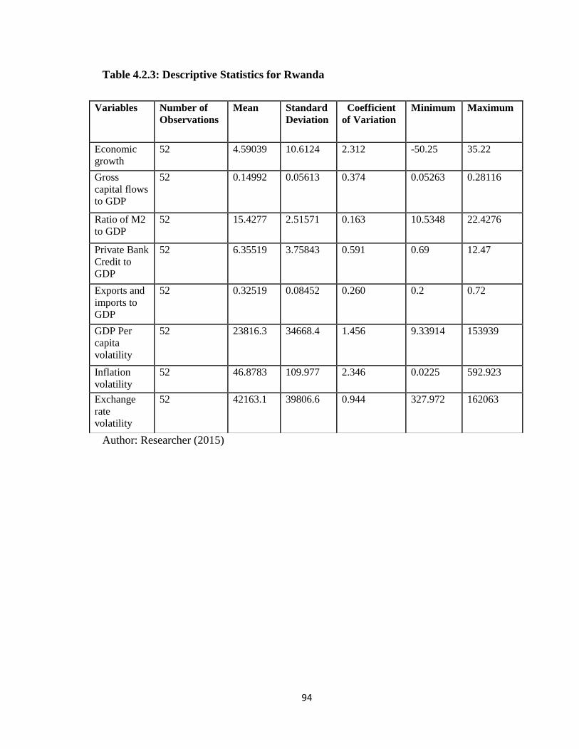
94

Table 4.2.3: Descriptive Statistics for Rwanda

Author: Researcher (2015)

Variables Number of

Observations

Mean Standard

Deviation

Coefficient

of Variation

Minimum Maximum

Economic

growth

52 4.59039 10.6124 2.312 -50.25 35.22

Gross

capital flows

to GDP

52 0.14992 0.05613 0.374 0.05263 0.28116

Ratio of M2

to GDP

52 15.4277 2.51571 0.163 10.5348 22.4276

Private Bank

Credit to

GDP

52 6.35519 3.75843 0.591 0.69 12.47

Exports and

imports to

GDP

52 0.32519 0.08452 0.260 0.2 0.72

GDP Per

capita

volatility

52 23816.3 34668.4 1.456 9.33914 153939

Inflation

volatility

52 46.8783 109.977 2.346 0.0225 592.923

Exchange

rate

volatility

52 42163.1 39806.6 0.944 327.972 162063

95

Figure 4.2.3: Trend Analysis on Rwanda

The economic growth for Rwanda experienced lower spike of -50 in the year 1994 and a

high spike in the year 1995. Exchange rate volatility oscillated in the value of 10 and had

a low spike in 1995. Both gross capital flows to GDP and trade integration oscillated in

the value of 0.

It is worth noting that, the per capita GDP had been declining as from 1989, one year

before the beginning of the war of 1990, up to 1994 from $360.87 in 1988 to $207.43 in

1994. Since 1995, the economic growth started to recover and currently, though the per

capita GDP is still low, Rwanda is among top performing economies in Africa with the

growth rate currently above both African and East African average. Several reasons

96

explain the underdevelopment of financial services. The weak culture of savings among

the people is due to low level of per capita income in the country. In fact, in 2009

Rwanda was ranked 21st poorest of the least developed countries in the world and 56.9

percent of its population lives on less than US$0.45 equivalent a day, the poverty

threshold in Rwanda (IMF, 2009).

The general poverty of the country can be attributed to being a landlocked country, bad

governance which has characterized the country since its independence, war and

insecurity, lack of natural resources, little skilled human capital, as per year 2005 (less

than 1% of the population had a tertiary education) and a low level of investment. The

development of the financial sector before the genocide of 1994 was slow. At the time,

only 3 commercial banks and 2 specialized banks operated with a total of less than 20

branches in the country, and one microfinance (UBPR) with around 146 branches. The

war which affected the banking sector heavily resulted to the closure of the Central bank

for four months.

4.2.4: Descriptive Statistics for Tanzania

Table 4.2.4 gives the descriptive statistics for Tanzania in which the mean economic

growth for Tanzania for the period 1963 to 2014 was 4.40 and the average gross capital

flow to GDP was 0.24. The ratio of M2 to GDP was on average 18.09 while the mean

private bank credit to GDP was 5.81. From these results, we can deduce that, Tanzania‘s

economy is more financially integrated than all the other member states of the East

African economy, despite of its relatively low economic growth. Its level of financial

deepening, as measured by the ratio of M2 to GDP also supports the above position.

97

This could imply that, the results from the ratio of M2 to GDP are largely attributed to the

large size of the economy while the case for the ratio of private credit to GDP could be

occasioned by relatively low private credit.

However, more robust findings, would require further probing on these two parameters.

In line with the comparatively low economic growth, Tanzania‘s level of trade

integration is low as indicated by the ratio of exports and imports to GDP which stands at

an average of 0.37. The mean GDP per capita volatility was 23384.01, 101.28 for

inflation volatility and exchange rate volatility was on average 293042.60. These

volatility results on Tanzania‘s economy indicate that, Exchange rate depicts the highest

variations while the rate of inflation depicts comparatively low variations. On the whole,

the macro-economic environment remains unstable due to low levels of trade and

economic development. This position is also supported by the high relative variability

values in GDP per capita volatility and exchange rate volatility (coefficient of variation

values of 1.53 and 1.07, respectively).

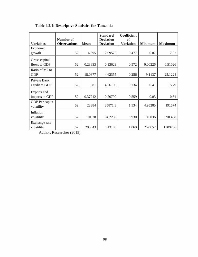
98

Table 4.2.4: Descriptive Statistics for Tanzania

Variables

Number of

Observations Mean

Standard

Deviation

Deviation

Coefficient

of

Variation Minimum Maximum

Economic

growth 52 4.395 2.09573 0.477 0.07 7.92

Gross capital

flows to GDP 52 0.23833 0.13623 0.572 0.00226 0.51026

Ratio of M2 to

GDP 52 18.0877 4.62355 0.256 9.1137 25.1224

Private Bank

Credit to GDP 52 5.81 4.26195 0.734 0.41 15.79

Exports and

imports to GDP 52 0.37212 0.20799 0.559 0.03 0.81

GDP Per capita

volatility 52 23384 35871.3 1.534 4.95285 191574

Inflation

volatility 52 101.28 94.2236 0.930 0.0036 390.458

Exchange rate

volatility 52 293043 313138 1.069 2572.52 1309766

Author: Researcher (2015)

99

Figure 4.2.4: Trend Analysis on Tanzania

Figure 4.2.4 above illustrates that, the economic growth had a wavy like shape which

initially ranged from 0 to 5 from the year 1963 to 1978 then oscillated around the value

of 5 but later on, from the year 2001 economic growth in Tanzania experienced a general

upward trend. The figure also displays that, gross capital flow to GDP and trade

integration was 0. In addition, exchange rate volatility lies in the range of 10 to15, save

for the years 1993 and 1994 in which the value was below 10. Inflationary volatility

oscillated around the value of 5, with 3 negative spikes in the years 1969, 1997 and 2012.

On the other hand, GDP per capita oscillated around the value of 10 with large

discrepancies in the years 1983, 1984, and 1997. Attribution analysis on this trend is

provided below.

100

Kaiser (1996) correctly attributes the emergence of the Arusha declaration to the failures

of the first five year plan that was adopted by Tanzania just after independence. The plan

was not yielding the anticipated results. Rural-urban development differentials increased,

local expertise remained inadequate and land and labour resources were underutilized.

According to Kaiser, ―Given these imbalances, President Julius Nyerere presented an

alternative vision in 1967 as outlined in the Arusha Declaration‖. According to Levin

(2001), during the period of Arusha Declaration per capita incomes grew by 0.70 per cent

per year. This was led by the public administration sector with a sizeable contribution

from agriculture and manufacturing. Exports stagnated due to the policy environment that

was hostile for exports. Government had monopoly on marketing of goods and services.

Inefficiencies drove down producer prices and there was high effective protection of the

import-substituting industrial sector. Trade controls, instead of exchange rate adjustment,

were used as a means of adjusting to external shocks. Suppression of private business

limited opportunities for entrepreneurship, control of prices, exchange rate, interest rate,

imports and exports added to the already hostile business and investment climate.

From the mid-1980s and especially from 1985, another major political decision was made

in Tanzania. Following the wind of change across the globe, the country adopted far-

reaching reforms in the management of its economy, inter- alia. This epoch therefore, can

be referred to as the reform era. These reforms were generally the opposite of the 1967

political decision to embrace socialism. In this epoch, Tanzania‘s political decision was

to embrace the capitalist, market-oriented and private- sector-led economic development

and change. The relatively free interplay of the market forces of supply and demand, and

101

correctly so, became the major defining characteristic of the country‘s economic

development and change.

A substantial political decision that negatively impacted Tanzania‘s economic

development in the 1967 to mid-1980s epoch was the 1978/79 war with Uganda. The

dictatorial political leadership of Iddi Amin in Uganda resulted into war over border in

Kagera region of Tanzania. The cost of waging war can be seen as the economic

development opportunity cost. The financial, human and time resources that are devoted

to war cannot at the same time be used for economic development. Destruction of

infrastructure and properties, time that civilians are unable to work optimally and lives

that are lost because of war, impact on economic development immensely.

4.2.5: Descriptive Statistics for Uganda

The mean economic growth for Uganda for the period 1963 to 2014 as illustrated in

Table 4.1.5 below was 4.20 and the average gross capital flow to GDP was 0.17. The

ratio of M2 to GDP was on average 15.59 while the mean private bank credit to GDP was

4.07. Uganda‘s ratio of exports and imports to GDP was on average 0.38.

These results indicate that, Uganda has a relatively low level of economic growth, a

position that is well supported by its low level of financial deepening as measured by

both the ratio of M2 to GDP and the ratio of private credit to GDP. However, the country

has been experiencing relatively high level of trade openness and financial openness. The

mean GDP per capita volatility was 14730.18, 12.53 for inflation volatility and exchange

102

rate volatility was on average 788579.60. Exchange rate depicts extremely high

variations compared to GDP per capita and the rate of inflation. However, based on the

coefficient of variation, inflation volatility and GDP volatility depict the highest relative

variability (2.38 and 1.43, respectively). This serves as evidence of instability in the

macro-economic environment; a situation cutting across all the East African community

member states.

Gavin and Hausmann (1996) studying on the sources of macroeconomic volatility in

developing countries over the period 1970-1992 found that, there is a significant positive

association between the volatility of capital flows and output volatility. These findings

are supported by these descriptive statistics as well as the correlation analysis results

presented later in this chapter. The consistent results on inflation volatility in all the

member states show that, inflation remains a key concern in these economies. Infact, the

results are consistent with the prevailing macro-economic conditions where, instability in

the general price levels continues to be experienced in these economies.

103

Table 4.2.5: Descriptive Statistics for Uganda

Author: Researcher (2015)

Variables

Number of

Observations Mean

Standard

Deviation

Coefficient of

Variation Minimum Maximum

Economic growth 52 4.21808 3.93585 0.933 -7.31 11.52

Gross capital flows

to GDP 52 0.1722 0.09562 0.555 0.0597 0.40026

Ratio of M2 to

GDP 52 15.589 5.62543 0.361 2.55887 26.1282

Private Bank Credit

to GDP 52 4.07346 3.63181 0.892 -0.29 13.75

Exports and imports

to GDP 52 0.37615 0.11399 0.303 0.17 0.62

GDP Per capita

volatility 52 14730.2 21020 1.427 17.2831 103994

Inflation volatility 52 12.5278 29.853 2.383 0.0001 190.164

Exchange rate

volatility 52 788580 705675 0.895 2348.37 3255932

104

Figure 4.2.5: Trend Analysis on Uganda

Figure 4.2.5 shows that, Uganda‘s economic growth was spiky for the entire period and

exhibited increasing trend. Gross capital flows to GDP and trade integration oscillated

around the value of 0. Exchange rate volatility lied in the range of 10 to 15 with an

exception of a low spike exhibited in the year 1991.GDP per capita volatility had wavy

like pattern which was in the range of 5 to 10, with an exception of low spikes in the year

1977, 1983, 1984, 1985, 1990, 1999 and 2000. The figure also shows that, inflation

volatility lied in the range of 0 to 5 with low negative spikes in the years 1963, 1967and

1971.The country‘s economic overview below extracted from the world bank website,

provides some insights into the above trend.

105

Starting in the late 1980s, the Uganda government pursued a series of impactful

liberalization policies. The resultant macroeconomic stability, post-conflict rebound, and

investment response to the pro-market reforms generated a sustained period of high

growth during 1987-2010. Real gross domestic product (GDP) growth averaged 7.00%

per year in the 1990s and the 2000s, making it one of the fastest growing African

countries. However, over the past decade, the country witnessed more economic volatility

and gross domestic product (GDP) growth slowed to an average of just about 5%. With

the population continuing to increase at a rate of 3.00% per annum, per capita income

growth has decelerated from a rate of 3.60% recorded in the decades of 1990s and 2002,

to about 2.00%. Beyond the risks relating to fiscal management in the face of election

related pressures, poor performance in the area of domestic revenue mobilization; and the

uncertainty regarding the date of commencement of oil production and the subsequent

flow of revenues, Uganda‘s growth and development is constrained by the low levels of

productivity of both agricultural and non-agricultural sectors; inappropriate urban

development; the slow development of infrastructure; and the limited availability of

credit (www.worldbank.org).

4.2.6 Comparative Observations on the Descriptive statistics

Burundi has generally experienced slow economic growth compared to the rest of the

region. This, has been attributed to low capital flows (to some extent) as indicated by the

average value of 0.12 compared to Tanzania at 0.24 and Kenya at 0.21; the biggest

economies in the region. The Kenyan economy depicts the best economic performance,

on average.

106

This position is supported by the relatively high capital flows (an average of 20.70% of

GDP), the highest level of financial deepening in the region (an average money supply of

31.53 of GDP and 21.00 private sector credit to GDP) as well as the highest level of trade

openness as measured by the ratio of imports and exports to GDP. The economic

performance of Rwanda was found to be the second highest in the region, after Kenya‘s

economy despite of lower capital flows (financial integration), lower financial deepening

as well as the level of trade openness compared to Tanzania and Uganda.

Tanzania‘s economy on the other hand, is more financially integrated than all the other

member states of the East African economy, despite of its lower economic growth, on

average (third best after Kenya and Rwanda). However, in line with the comparatively

low economic growth, Tanzania trails Kenya and Uganda in terms of the level of trade

openness as indicated by the ratio of exports and imports to GDP which stands at an

average of 0.37. These results also indicated that, Uganda has the second lowest level of

economic growth, a position that is well supported by its low level of financial deepening

as measured by both the ratio of M2 to GDP and the ratio of private credit to GDP.

However, the same economy has the second highest level of trade openness and the third

highest level of financial openness, implying that, the country is much more

economically integrated than Rwanda and Burundi. (More details are presented

graphically in appendices iii to viii).

Partly, the war between some of the East African countries (Tanzania and Uganda), tribal

clashes and political violence contributed to the seasonal dismal performance of the East

African member states. Infact, the literature on the impacts of war on economic

107

development is abundant and strongly supports this position. Among these include Ades

and Chua (1997) who found that, regional instability and domestic political instability

have strong negative effects on a country‘s economic performance. This takes place

through reduced trade within and between unstable regions and countries; increased

military and defense expenditure; they also found that government expenditure on

education was lower in countries with politically unstable neighbours. Glick and Taylor

(2005) studied the effects of war on bilateral trade for almost all countries with available

data extending back to 1870. They found large and persistent impacts of wars on trade,

and hence on national and global economic development and welfare. Similar findings

are documented in Anderton and Carter (2001), who studied the impact of war on trade

for 14 major power dyads and 13 non-major power dyads.

4.3 Multicollinearity Test

Before carrying out the correlation analysis, multicollinearity test was conducted to

establish the possibility and extent of linear dependence between the study variables. The

details are provided below.

The results presented in Table 4.3 below shows that, the mean variance inflation factor

(VIF) was estimated at 1.47, which is greater than the critical value of 1. It‘s called the

VIF because it estimates how much the variance of a coefficient is ―inflated‖ because of

linear dependence with other predictors. Thus, a VIF of 1.47 tells us that the variance (the

square of the standard error) of a particular coefficient is 47% larger than it would be, if

that predictor was completely uncorrelated with all the other predictors.

108

As indicated in Table 4.3, no VIFs were greater than 10. This demonstrates absence of

strong multicollinearity. In addition, the variables with high VIFs are private bank credit

to GDP and M2/GDP which are control variables, and the variables of interest do not

have high VIFs. Hence we can safely ignore multicollinearity. Measures of distribution

such as skewness and kurtosis which are usually incorporated in the Jargue Bera statistic

for normality test were not computed. The reason for omitting these measures was

because the assumption of a normally distributed error term is held in estimation under

ordinary least squares (OLS). However, this study utilized the generalized two-stage least

square (G2SLS) random-effects instrumental variable method (REIVM).

Table 4.3: Variance Inflation Factor (VIF) Test for Multicollinearity

Author: Researcher (2015)

Variable VIF 1/VIF

Private Bank Credit to GDP 2.02 0.4955

M2/GDP 1.79 0.5589

Trade integration 1.66 0.6016

Gross capital flow to GDP 1.58 0.6313

Exchange rate volatility 1.13 0.8852

GDP per capita volatility 1.1 0.9050

Inflation volatility 1.02 0.9776

Mean VIF 1.47

109

4.4 Correlation Analysis

The researcher proceeded to analyze the correlation between each of the variables to

ascertain the direction of association and its statistical significance as presented in table

4.4 below, after the discussion of the results.

4.4.1 Economic Growth and Financial Integration

Gross capital flow to GDP (financial openness) is positively and significantly correlated

to economic growth (r=0.2093, p <0.05). These findings were similar to those established

by Edison et al (2002) who concluded that, international financial integration is positively

associated with real per capita. Njoroge (2010) arrived at similar findings that, economic

integration had a positive and significant impact on economic growth. Blomstrom et

al(1994), Quinn (1997), Borenzstein, De Gregorio, and Lee (1998)), Alfaro, Chanda,

Kalemli-Ozcan, and Sayek (2003) arrived at similar findings, as well.

4.4.2 Economic Growth and Macro-economic Volatility

Two measures of macroeconomic volatility, namely, GDP per capita volatility (r=

0.0662, p >0.05) and exchange rate volatility (r = 0.054, p > 0.05) were positively

correlated to economic growth though not statistically significant. However, inflation

volatility was negatively correlated to economic growth even though not statistically

significant (r =-0.089, p>0.05). Hence the three measures of macroeconomic volatility

had a correlation value which was statistically not different from 0. These results differ

from the findings by Hnatkovska and Loayza (2003) who concluded that, macroeconomic

volatility and long-run economic growth are negatively related. Rajmund et al (2015),

110

also arrived at similar findings, showing stronger relationship in developing countries

than developed countries.

4.4.3 Financial Integration and Financial Deepening

The table shows that, the two measures of financial deepening, namely, ratio of M2 to

GDP (r= 0.3707, p < 0.05) and private bank credit to GDP (r = 0.3606, p <0.05) are

positively and significantly correlated to financial openness. The two measures are used

as control variables in this study.

4.4.4 Financial Integration and Trade Integration

Table 4.2 also shows that, the measure of trade integration, namely, total exports and

imports to GDP is positively and statistically significantly related to financial openness (r

=0.5960, p <0.05). However, trade integration though positively correlated to economic

growth, was not supported by statistical test of significance. This findings support Lane

(2000); Heathcote and Perri (2004) assertion that, though not directly linked, it has been

proved that, countries which are more open to trade are also more open financially.

4.4.5 Financial Integration and Macro-economic Volatility

The table on pairwise correlation analysis further displays that, all the three measures for

macroeconomic volatility were positively correlated to financial openness, although only

GDP per capita volatility and exchange rate volatility had correlation values which were

statistically different from 0 (r =0.1975 , p < 0.05) and ( r =0.4114, p < 0.05). The results

conform to those established by O‘Donnell (2001) in non-OECD countries that a higher

111

degree of financial integration is associated with higher output volatility. However, the

findings differ from those by O‘Donnell (2001) in OECD countries that a higher degree

of financial integration is associated with lower output volatility. Similarly, the findings

deviate from those by Easterly, Islam and Stiglitz (2001) who found that, a higher level

of development of the domestic financial sector is associated with lower volatility.

Mendoza (1994), Backus, Kehoe, Kydland (1995) and Baxter and Crucini (1995)

findings are also different from the findings of the current study.

4.4.6 Trade Integration and Macro-Economic Volatility

Similar findings were deduced on the correlation between macroeconomic volatility and

trade integration, in which GDP per capita volatility and exchange rate volatility were

positively and significantly correlated to trade integration (r =0.3068, p < 0.05) and ( r

=0.1565, p < 0.05). Similar findings were deduced by Easterly, Islam and Stiglitz (2001)

that an increase in the degree of trade openness leads to an increase in the volatility of

output, especially in developing countries. This indicates that, the association between

macroeconomic volatility and either financial openness or trade integration depends on

the macroeconomic volatility measure adopted. These results conform to those by Razin

and Rose (1994) who indicate that, the impact of trade integration on volatility is

ambiguous in theory.

112

Table 4.4: Pairwise Correlation coefficients for the Variables

Economic

growth

Gross

capital

flows

to GDP

Ratio

of M2

to GDP

Private

Bank

Credit

to GDP

Exports

and

imports

to GDP

GDP

Per

capita

volatility

Inflation

volatility

Exchange

rate

volatility

Economic

growth 1

Gross capital

flows to

GDP 0.2093* 1

0.0007

Ratio of M2

to GDP 0.016 0.3707* 1

0.7974 0.0000

Private Bank

Credit to

GDP 0.039 0.3606* 0.8333* 1

0.5317 0.0000 0.0000

Exports and

imports to

GDP 0.0124 0.5960* 0.6487* 0.6224* 1

0.8419 0.0000 0.0000 0.0000

GDP Per

capita

volatility 0.0662 0.1975* 0.3628* 0.4112* 0.3068* 1

0.2877 0.0014 0.0000 0.0000 0.0000

Inflation

volatility -0.089 0.0903 0.0926 0.0299 0.0987 -0.0275 1

0.1523 0.1466 0.1366 0.6317 0.1122 0.6593

Exchange

rate volatility 0.054 0.4114* -0.0468 -0.0758 0.1565* 0.0268 -0.0874 1

0.386 0.0000 0.4525 0.2232 0.0115 0.6673 0.1598

* denotes statistical significance at the 5 percent level

Author: Researcher (2015)

4.5 Unit Root Tests

Before estimating the different models to address the study objectives, panel unit root test

was first conducted to establish whether there were any variables in the model that were

113

non-stationary. The Im- Pesaran-shin Test (IPS) panel unit root test was conducted. The

IPS estimates the t-test for unit roots in heterogenous panels (Wicks-Lim, 2005). The test

allows for individual effects, time trends and common time effects. It is based on the

mean of the individual Dickey-Fuller (DF) t-statistics of each unit in the panel, and

assumes that all series are non-stationary (have unit roots) under the null hypothesis.

Table 4.5 gives the summary of the unit root test based on the IPS Test.

Table 4.5: IPS Panel Unit Root Tests

t-bar Statistic

Variable Levels

First

difference

Levels with

time trend

Gross capital flows to GDP (Financial openness) -1.9586 -9.6123* -2.8170*

M2/GDP (Financial Deepening 1) -2.4817* -9.6148* -3.5410*

Private Bank Credit to GDP

(Financial Deepening 2)

-0.6178

-12.3860* -2.2957*

GDP Per capita volatility -2.0085 -4.7559* -2.2944*

Inflation volatility -4.9621* -9.5239* -5.0659 *

Exchange rate volatility -0.9297 -4.4846* -1.7075

Trade Integration -2.9090* -10.2997* -3.5819*

Economic growth -5.2093* -10.6814* -5.8813*

* denotes statistical significance at the 5 percent level

Author: Researcher (2015)

114

In the test results presented in Table 4.5, gross capital flows to GDP was non-stationary

in levels. Similarly, the ratio of private bank credit to GDP was also non-stationary at

levels. In addition, two measures for macro-economic volatility namely GDP per capita

volatility and exchange rate volatility were also non-stationary at levels. However, after

including a time trend gross capital flows to GDP, private bank credit to GDP, and GDP

per capita volatility attained stationarity, showing that the three variables were trend

stationary. Furthermore, all the non-stationary variables became stationary upon

conducting the first difference of the variables. Hence, the variable exchange rate

volatility was difference stationary.

4.6 Rationalizing the choice of model

The data used in this study is panel data. There are two types of models used in carrying

out regression analysis with panel data: fixed effects and random effects models. Fixed

effects regression is used to control for omitted variables that differ between the countries

but are constant over the time period 1963 to 2014. However, some omitted variables

may be constant over the given time period but vary between the countries. Other

variables may be fixed between the countries but vary over time. One can include both

types of variables which vary between countries and also over time by using random

effects model.

Statistically, estimation of a fixed effects model is always a reasonable thing to do in

panel data estimation. This is because fixed effects models give consistent results such

that, as the sample size increases indefinitely, the estimated parameters converge to their

115

true values. The fixed effects models may, however, not be the most efficient (have

minimum variance) model to run. Since, studying the entire population is expensive and

time-consuming, consistency ensures that, the sample being surveyed represents reality of

what is taking place in the entire population, while efficiency ensures there are minimal

variations between observed characteristics under investigation. Random effects will give

better P-values (higher chances of finding that various policy options do influence

economic growth) as they are a more efficient estimator, so one should run random

effects if it is statistically justifiable to do so.

Table 4.6: Hausman Test for fixed effects and random effects models

Economic Growth Fixed Effects Model Random Effects Model Difference

Financial openness 0.3825 -2.3468 2.7292

Trade Integration -2.0873 -1.1150 -0.9724

GDP per capita volatility 1.07E-06 1.10E-06 -3.39E-08

Chi-Square Statistic 0.03 P-Value 0.9851

Financial openness 56.7677 54.7599 2.0079

Trade Integration -1.8568 -0.4960 -1.3608

Inflation Volatility -5.78E-03 -5.74E-03 -4.09E-05

Chi-Square Statistic 0.73 P-Value 0.8665

Financial openness 58.4319 54.6107 3.8211

Trade Integration -5.1068 -1.7752 -3.3316

Exchange Rate Volatility 2.03E-06 9.97E-07 1.03E-06

Chi-Square Statistic 2.47 P-Value 0.2913

Author: Researcher (2015)

116

4.6.1 Hausman Test for fixed effects and random effects models

Under the Hausman (1978) test, the null hypothesis is that the coefficients estimated by

the efficient random effects estimator are the same as the ones estimated by the consistent

fixed effects estimator. The Hausman (1978) test, therefore, checks a more efficient

model against a less efficient but consistent model to make sure that, the more efficient

model also gives consistent results. A summary of the Hausman (1978) test results are

presented in Table 4.6 above.

The test results show that, the Chi-square statistics for the difference were 0.03, 0.73 and

2.47 with corresponding p-values of 0.9851, 0.8665 and 0.2913 respectively. Since the p-

values were larger than the critical value of 0.05, hence the null hypothesis that, the

differences in the coefficients are not systematic was not rejected. This means that, the

preferred model was the random effects model. Hence the empirical results on hypothesis

testing presented in chapter five below are based on the random effects model.

4.7 Chapter Summary

On correlation analysis, Gross capital flow to GDP (financial integration) is positively

and significantly correlated to economic growth (r=0.2093, p <0.05). GDP per capita

volatility (r= 0.0662, p >0.05) and exchange rate volatility (r = 0.054, p > 0.05) were

positively correlated to economic growth though statistically insignificant. However,

inflation volatility was negatively correlated to economic growth even though not

statistically significant (r= -0.089, p>0.05). Financial deepening as measured by the ratio

117

of M2 to GDP (r= 0.3707, p < 0.05) and private bank credit to GDP (r = 0.3606, p <0.05)

are positively and significantly correlated to financial openness.

The correlation analysis on the association between financial integration and the other

variables indicated that, trade integration as measured by total exports and imports to

GDP is positively and statistically significantly related to financial openness (r =0.5960,

p <0.05). However, trade integration though positively correlated to economic growth,

was not supported by statistical test of significance.

On the association between financial integration and macro-economic volatility, all the

three measures for macroeconomic volatility were positively correlated to financial

openness, although only GDP per capita volatility and exchange rate volatility had

correlation values which were statistically different from 0 (r =0.1975 , p < 0.05) and ( r

=0.4114, p < 0.05). These results conformed to those established by O‘Donnell (2001) in

non-OECD countries that a higher degree of financial integration is associated with

higher output volatility. Similar findings were deduced on the correlation between

macroeconomic volatility and trade integration, in which GDP per capita volatility and

exchange rate volatility were positively and significantly correlated to trade integration

((r =0.3068, p < 0.05) and ( r =0.1565, p < 0.05). The findings are similar to those

established by Easterly, Islam and Stiglitz (2001). Hausman Test for fixed effects and

random effects models indicated that, the preferred model was the random effects model,

which is applied in testing the hypothesis in the next chapter.

118

CHAPTER FIVE

HYPOTHESES TESTING AND DISCUSSION OF FINDINGS

5.1 Introduction

This study sought to investigate on the influence of macroeconomic volatility and trade

integration on the relationship between financial integration and economic growth in the

EAC. Section 5.2 provides the discussion of findings from the test of hypothesis while

section 5.3 provides comparative analysis between the expected relationships and the

actual findings.

5.2 Hypotheses Testing and Discussion of Findings

To achieve the set objectives, the following five hypotheses (accordingly numbered) were

tested.

Hypothesis 1: Financial integration has no significant effect on economic growth.

In order to address the first hypothesis of this study, the dependent variable (economic

growth) was regressed against gross capital flow to GDP as the explanatory variable.

However, instruments for financial deepening, namely, the ratio of M2 to GDP and the

ratio of bank credit to the private sector to GDP were included, hence the generalized

two-stage least square (G2SLS) random-effects instrumental variable (IV) was used as

the regression model as presented in table 5.1.

119

Table 5.1: Financial Integration and Economic Growth

Author: Researcher (2015)

A positive coefficient of 4.40 on gross capital flow to GDP was realized with a p-value of

0.662 which was not statistically significant at the 0.05 level. Hence we fail to reject the

hypothesis that, financial integration has no significant effect on economic growth. This

indicates that, financial integration as measured by gross capital flow to GDP is

positively associated with economic growth, though it does not have a statistically

significant effect on economic growth. The study findings are similar to those by Edison

et al (2002) that, international financial integration does not support the view that

promotes economic growth, though international financial integration is positively

associated with real per capita.

G2SLS-REMIV

Economic growth Coefficient Z P-Value

Gross capital flow to GDP 4.40 0.44 0.662

Constant 3.3911** 1.84 0.066

R-squared: Within 0.0398

Between 0.3898

Overall 0.0438

Chi-square statistic 0.19

0.6623

Instrumented: Gross capital flow to GDP

120

This model means that, the East African member states can achieve an economic growth

rate of 3.3911% in the absence of financial integration and this growth rate can increase

by 4.4% for every 1% increase in the level of financial integration. Essentially, the

presence of financial integration accelerates economic growth.

The R2 values indicate that, 3.98% of the variations in economic growth, as measured by

GDP per capita, within the countries are explained by financial integration, as measured

by the ratio of gross capital flows to GDP, 38.98% of the variations in economic growth

between the countries are explained by financial integration while 4.38% of the variations

in economic growth of the East African community as an economic bloc (considering

panel data) are explained by financial integration. This would mean that, overall, 95.62%

of the variations in economic growth of the East African community are explained by

other factors, other than financial integration, which are not accounted for, in the model

above.

The results imply that, the presence of financial integration in an economy leads to

improved economic growth. Further, these findings confirm the theoretical relationship

documented in the literature and justify the correlation results achieved in 4.3.1,

explaining the positive significant association between financial integration and

economic growth. The results are also supported by similar findings on the descriptive

statistics for the various East African member states (4.1) which indicated that, Kenya

had the highest average economic growth rate as well as the highest level of financial

integration.

121

By implication, countries with low level of financial integration or without financial

integration are faced by low levels of economic growth compared to the countries with

relatively higher levels of financial integration. An investigation into what determines

the effects of financial integration on economic growth reveals that, the composition of

capital flows determines the effects of financial integration on economic growth (Reisen

and Soto, 2001) and Goldberg, 2004). In particular, these studies conclude that, FDI

flows tend to be positively associated with output growth in those countries that have a

sufficient level of human capital (Borenzstein, De Gregorio, and Lee, 1998) and well-

developed domestic financial markets (Alfaro, Chanda, Kalemli-Ozcan, and Sayek,

2003). The East African financial markets are far from being developed although human

capital is reasonably sufficient. This explains why the regional Economic bloc (East

African financial markets) has low levels of gross capital. But what determines the

composition of capital flows?

The composition of capital flows is influenced by a number of factors, key among them;

Macroeconomic performance, Quality of institutions, Investment environment, financial

development, infrastructure and resources. The argument is that, a rapidly growing

economy is likely to offer higher future earnings and thus higher rates of return coupled

with lower risk. Based on the descriptive statistics discussed in chapter four, the East

African economic bloc economic performance is average, but remains below the targeted

level of 7%, for macro-economic convergence to take place. Theoretical and empirical

findings suggest that good institutions help promote capital inflows (Wei and Wu, 2001).

122

A country that ranks high in terms of law and order is expected to attract more capital

flows (Alfaro and others, 2003). The openness of the economy, the degree of exchange

rate and inflation volatility, and exchange controls are three key ingredients of the

investment environment. A positive relationship between FDI and openness is well

established in the literature (Asiedu, 2002; Morisset, 2000). In contrast, the relationship

between portfolio flows and trade openness is less clear, and the degree of trade openness

may be expected to play a small role. Exchange rate volatility increases the uncertainty of

demand for products of export oriented firms and may reduce the profitability of FDI. It

is, therefore, expected to have an adverse impact on FDI (Goldberg and Kolstad, 1994;

Kamaly, 2002). Its impact on portfolio flows is less clear. Inflation volatility is another

important source of uncertainty for foreign investors (Rogoff and Reinhart, 2003) and is

expected to have a negative effect on FDI. This explains why the gross capital flows in

East Africa is low relative to the Gross domestic product.

Both the quality of the infrastructure and the availability of resources determine the

attractiveness of a location. A well-developed infrastructure facilitates communication

with parent companies abroad and the information-gathering process for business and

reduces distribution costs, thus promoting local and regional trade. On financial

development, the deeper a country‘s financial markets, the more capital flows the country

attracts. In particular, well-developed financial markets appear to be a precondition for

portfolio inflows (Garibaldi and others, 2002). East African financial markets lack depth,

as indicated by the low private sector credit to GDP ratios displayed in the descriptive

statistics. This contributes directly to the low gross capital flow to GDP ratios, as well.

123

The findings above do not support the new economic integration theory and optimum

currency area theory, which were used to explain the direct relationship between financial

integration and economic growth.

Hypothesis 2: Macro-economic volatility does not have a significant moderating effect

on the relationship between financial integration and economic growth.

This involved testing the main effects of the independent variable (gross capital flow to

GDP), the moderating variable (each of the three measures of macroeconomic volatility)

and the interaction term between gross capital flow to GDP and each of the three

measures of macroeconomic volatility on the dependent variable (economic growth). In

order to create an interaction term, gross capital flow to GDP and each of the three

measures of macroeconomic volatility were multiplied. The creation of a new variable by

multiplying the scores of gross capital flow to GDP and each of the three measures of

macroeconomic volatility risks creating a multicollinearity problem. To address the

multicollinearity problem, which can affect the estimation of the regression coefficients

for the main effects, the interactive factors were converted to standardized (Z) scores that

have mean zero and standard deviation one. The standardized variables (gross capital

flow to GDP and each of the three measures of macroeconomic volatility) were then

multiplied to create the interaction variable.

The results of hierarchical multiple regressions predicting economic growth from gross

capital flow to GDP, each of the measures of macroeconomic volatility and the

interaction between gross capital flow to GDP are reported in models 1a to 1c. In the

second step, the interaction term between gross capital flow to GDP and each of the three

124

measures of macroeconomic volatility was entered into the regression equation and tests

of the slope was performed as reported in models 2a to 2c. However, the interaction term

was not statistically significant (p>0.05) in all the models, indicating that each of the

three measures of macroeconomic volatility has no moderation effect on the relationship

between gross capital flow to GDP and economic growth. The results are summarized in

tables 5.2, 5.3 and 5.4 below.

Table 5.2: Financial Integration, GDP per capita volatility and Economic Growth

Author: Researcher (2015)

Hnatkovska and Loayza (2003), conclude that macroeconomic volatility and long-run

economic growth are negatively related. This negative link is exacerbated in countries

that are poor, institutionally underdeveloped, undergoing intermediate stages of financial

development, or unable to conduct countercyclical fiscal policies. Lin and Kim (2014)

investigated the relationship between output volatility and growth using a simultaneous

equation system with a panel of 158 countries. They found a negative relationship and

also significant feedback between volatility and economic growth. However, this

G2SLS-random-effects IV regression Model 1a Model 2a

Economic growth

Coefficient

( P-Value)

Coefficient

( P-Value)

Gross capital flow to GDP -0.029 (0.998) -0.045 (0.997)

GDP per capita volatility 0.000 (0.361) 0.000 (0.448)

Normalized (Gross capital flow to GDP)*

Normalized (GDP per capita volatility)

0.080 (0.909)

Constant 4.024** (0.051) 4.025* (0.046)

R-squared: Within 0.0016 0.0018

Between 0.467 0.4641

Overall 0.0042 0.0042

Chi-square 1.13 (0.568) 1.14 (0.767)

Instrumented: Gross capital flow to GDP

125

feedback is doubtful as Jetter (2014) and Baker et al (2011) provided evidence that,

volatility tends to affect growth and not vice versa.

Macroeconomic volatility is caused by the interaction of shocks, both domestic and

external in origin, with economic institutions and policy regimes that are ill-adapted to

the volatile environment with which they must deal. While terms of trade and other

external shocks appear to matter, policy is the most important determinant of the

volatility of macroeconomic outcomes. We find that, monetary volatility, exchange-rate

regimes, and measures of political instability are particularly important determinants of

the volatility of real GDP growth and of the real exchange rate. Monetary volatility is, in

turn, associated with volatile fiscal deficits and shallow domestic financial markets. This

is characteristic of the East African economic bloc.

Table 5.3: Financial Integration, Inflation Volatility and Economic Growth

G2SLS-random-effects IV regression Model 1b Model 2b

Economic growth

Coefficient

( P-Value)

Coefficient

( P-Value)

Gross capital flow to GDP 5.586 (0.582) 5.955 (0.541)

Inflation volatility -0.005 (0.123) -0.005 (0.115)

Normalized (Gross capital flow to GDP)*

Normalized (Inflation volatility)

0.108 (0.823)

Constant 3.466 (0.057) 3.395** (0.052)

R-squared: Within 0.0418 0.0427

Between 0.5412 0.5106

Overall 0.0472 0.0481 Chi-square 2.42 (0.298) 2.69 (0.442)

Instrumented: Gross capital flow to GDP

Author: Researcher (2015)

126

Inflation volatility is another important source of uncertainty for foreign investors

(Rogoff and Reinhart, 2003) and is expected to have a negative effect on FDI. Because

some portfolio flows are short term, the effect of inflation volatility on them may be

smaller than on FDI or even negligible. Supply shocks explain about 45 percent (while

demand shocks explain about 45 percent) of the inflation fluctuations in the Sub-Saharan

region on average, one-third of which reflect shocks to global commodity prices and

inflation spillovers from other countries, and the other two-thirds reflect other supply

shocks to inflation such as weather-related shortfalls. Shocks to global oil and food prices

explain about 7 percent of inflation fluctuations in the region.

In general, global commodity prices contribute more to inflation in economies that have

higher oil intensity (defined as a kilogram of oil equivalent per capita). Foreign inflation

spillovers are also important in driving inflation with a contribution of 8 percent on

average, reflecting imported inflation from other countries. As expected, the importance

of foreign inflation spillovers generally increases with higher import.

Table 5.4: Financial Integration, Exchange Rate Volatility and Economic Growth

Author: Researcher (2015)

G2SLS-random-effects IV regression Model 1c Model 2c

Economic growth

Coefficient

( P-Value)

Coefficient

( P-Value)

Gross capital flow to GDP 4.999 (0.596) 2.468 (0.822)

Exchange rate volatility 0.000 (0.808) 0.000 (0.923)

Normalized (Gross capital flow to GDP)*

Normalized (Exchange rate volatility )

0.228 (0.572)

Constant 3.209* (0.036) 3.688* (0.045)

R-squared: Within 0.0364 0.0208

Between 0.2667 0.1730

Overall 0.0388 0.0225 Chi-square 1.05 (0.591) 1.61 (0.658)

Instrumented: Gross capital flow to GDP

127

Political instability, as measured by the incidence of revolutions and coups, is also an

important determinant of real exchange-rate volatility. This is not hard to understand:

when there is political trouble, money is the first thing to fly across the border. This puts

pressure on both the nominal and the real exchange rates. Terms-of-trade changes are

also key factors driving exchange rates movements, although the impact varies widely

across the region. The rise in food and fuel prices has led to higher import bills and

significant balance of payment gaps, triggering fast depreciation and high volatility of

currencies in net importing countries such as Kenya, Tanzania and Uganda.

Hau (2002) states that, the theoretical linkage between openness and real exchange rate

volatility depends on the magnitude of the monetary and real shocks of each country.

This suggests that, analysing the sources of exchange rate volatility at a country level will

likely be better for formulation of the correct type of policy response(s). Furthermore,

they measure exchange rate volatility using very low frequency data (i.e. yearly data) yet

exchange rate volatility will be best measured using either very high frequency data (i.e.

intraday or daily data) or low frequency data (i.e. monthly or quarterly data).

The hegemonic stability theory while supporting the optimum currency area and the new

economic integration theory, was used to explain the moderating effect of macro-

economic volatility on the relationship between financial integration and economic

growth. Hegemonic stability theory indicates that, the international system is more likely

to remain stable when a single nation-state is the dominant world power, or hegemon

(Joshua, 2005). Thus, the fall of an existing hegemon or the state of no hegemon

128

diminishes the stability of the international system. The findings above did not support

this theory, given the high macro- economic volatility in the East African region,

discussed in chapter four. This points to the state of no hegemon in the East African

community.

Hypothesis 3: Trade integration does not have a significant intervening effect on the

relationship between financial integration and economic growth.

This involved testing the main effects of the independent variable (gross capital flow to

GDP) and the intervening variable (trade integration). This was done in four steps as

indicated in tables 5.5 and 5.6 below.

Table 5.5: Financial Integration, Trade Integration and Economic Growth

Author: Researcher (2015)

G2SLS-random-effects IV regression Step 1Model 1d Step 2 Model 2d

Coefficient

( P-Value)

Coefficient

( P-Value)

Regressand Economic growth Trade integration

Gross capital flow to GDP 4.40 (0.662) 1.07*(0.000)

Trade integration

Constant 3.3911**(0.066) 0.205 (0.000)

R-squared: Within 0.0398 0.4296

Between 0.3898 0.2559

Overall 0.0438 0.3552

Chi-square 0.04 (0.980) 72.55* (0.000)

Instrumented: Gross capital flow to GDP

129

Table 5.6: Financial Integration, Trade Integration and Economic Growth

Author: Researcher (2015)

The results of hierarchical multiple regression predicting economic growth from gross

capital flow to GDP are reported in table 1d. The results indicate that, Gross capital flow

to GDP (the independent variable) is not significant. The regression of the intervening

variable (trade integration) on Gross capital flow to GDP is reported in step 2 model 2d.

The results show that, Gross capital flow to GDP is significant, implying that Gross

capital flow to GDP (financial integration) affects trade integration. Model 3d presents

the regression of trade integration on economic growth. The findings indicate that, the

regressor variable is not significant.

Since, more than one (model 1d and model 3d) of these relationships are not significant,

we conclude that, mediation is not possible or likely. However, a confirmation test was

done in step 4 model 4d in which economic growth was regressed on both Gross capital

G2SLS-random-effects IV regression Step 3 Model 3d Step 4 Model 4d

Coefficient

( P-Value)

Coefficient

( P-Value)

Regressand Economic growth Economic growth

Gross capital flow to GDP

-12.76 (0.948)

Trade integration 0.477 (0.842) 5.14 (0.942)

Constant 3.99*(0.000) 4.42 (0.511)

R-squared: Within 0.001 0.0816

Between 0.2821 0.0088

Overall 0.0002 0.0624

Chi-square 0.04 (0.842) 0.04 (90.98)

Instrumented: Gross capital flow to GDP

130

flow to GDP and trade integration. None of the regressors was found to be significant.

This results confirm the finding in step 1 and step 3, that trade integration has no

intervening effect on the relationship between financial integration and economic growth.

An Optimum Currency Area (OCA) is a geographical region in which it would maximize

economic efficiency to have the entire region share a single currency. The theory was

used to explain the intervening effect of trade integration on the relationship between

financial integration and economic growth. Proponents of this theory argue that, potential

MUs should exhibit similarity in economic structure characterized by high degree of

wage flexibility to allow for the adjustment of asymmetric shocks; a high degree of

labour mobility; and a high degree of goods and market integration across States. The

size and openness of the economy, degree of commodity diversification and fiscal

integration are also important to the formation of a successful MU (Mckinnon, 1963;

Kenen, 1969; Flemming (1971).

In 2010 the East African Community (EAC) Common Market became operational and

introduced the free movement of workers therefore enabling citizens of EAC to work

anywhere within the member countries without discrimination. The free movement of

workers was to be implemented gradually for a period of 5 years and become fully

operational by 2015. Semboja (2005) indicates that, EAC has a challenge of balancing

professional labour mobility bearing the inequilibrium level of education in the member

states. However, according to Kasekende, (2009), EAC should design incorporated

employment-generating macroeconomic rules that create decent job openings for young

131

women and men, who are the majority of the population, hence overcoming the problem

of one nation getting more advantage than the other due to education levels and

subsequently allowing smooth professional labour mobility. Onduko (2013) sought to

study on regional integration and professional labour mobility in East Africa. She

concluded that, the impact of the Common Market on free movement of workers has not

yet been felt on the ground because there are many challenges and it is not fully

implemented yet. Therefore, free movement of workers is not free at all in East Africa.

This means that, the degree of labour mobility is not high, hence contributing to the

inefficiency of the economic bloc.

Economic structures of the EAC countries are generally diverse in terms of incomes,

industrial structures, and social indicators with similarities in few areas. The agricultural

sector accounts for 23 to 35 percent of the economy in all five countries. Coffee and tea

are major exports for Burundi, Kenya, Rwanda, and Uganda. While Tanzania exports

mostly gold, tobacco, and coffee, Kenya exports horticultural products as well. Kenya,

Tanzania, and Uganda have more diversified exports in recent years. Regarding the

financial sector, although there is some differentiation, domestic debt markets are largely

underdeveloped with low savings rates and limited investor base. Wang (2010) presents

preliminary evidence suggesting that EAC members are financially less open when

compared with advanced economies. Moreover, within the EAC, Kenya is the most

financially open economy, followed by Uganda and Tanzania.

132

Several challenges remain in the form of non-tariff barriers preventing freer movement of

goods and services. Roadblocks, delays at border posts, and inconsistent import and

export standards are some examples of the existing restrictions clouding prospects for

further trade integration within the EAC. Aware of these problems, EAC countries agreed

to work together to strengthen customs administration; pursue trade facilitation through

harmonized and simplified customs procedures; enhance revenue management by

improving EAC tariff regimes and rules of origin; promote custom and trade

partnerships; and enhance market access, trade and competitiveness including

harmonization of administrative procedures and regulations.

Hypothesis 4: Financial integration, macroeconomic volatility and trade integration do

not have a joint effect on economic growth.

To establish the joint effect of financial integration, macroeconomic volatility and trade

integration on economic growth, the G2SLS random-effects instrumental variable

regression model was utilized to access these relationships. However, three models were

estimated which differed only on the measure for macro-economic volatility.

133

Table 5.7: Financial integration, GDP per Capita Volatility and Trade Integration

on Economic Growth

Source: Researcher (2015)

The test for the joint effect of the explanatory variables on economic growth in the first

model used GDP per capita volatility as a measure of macro-economic volatility as

reported in Table 5.7. A chi-square statistic of 1.19 was produced with a corresponding p-

value of 0.76 which was statistically not significant at the 0.05 level of significance.

Hence, we fail to reject the hypothesis showing that, financial integration, GDP per capita

volatility and trade integration do not have a joint effect on economic growth. This shows

that, the included explanatory variables do not have a joint effect on economic growth.

The R2 values indicate that, 5.46% of the variations in economic growth, as measured by

GDP per capita, within the countries are explained by the joint effect of financial

integration, GDP per capita volatility and trade integration, 26.71% of the variations in

G2SLS-REMIV

Economic growth Coefficient Z P-Value

Gross capital flow to GDP 6.54117 0.04 0.966

Trade integration -2.70469 -0.05 0.961

GDP per capita volatility 5.73e-06 0.89 0.374

Constant 3.9184 0.73 0.468

R-squared: Within 0.0546

Between 0.2671

Overall 0.0563

Chi-square Statistic 1.19

0.7560

Instrumented: Gross capital flow to GDP

Instruments:

Trade integration

GDP per capita volatility

134

economic growth between the countries are explained by the joint effect of financial

integration, GDP per capita volatility and trade integration while 5.63% of the variations

in economic growth of the East African community as an economic bloc (considering

panel data) are explained jointly by financial integration, GDP per capita volatility and

trade integration.

Table 5.8 Financial integration, Inflation Volatility and Trade Integration on

Economic Growth

G2SLS-REMIV

Economic growth Coefficient Z P-Value

Gross capital flow to GDP 55.673 0.71 0.480

Trade integration -20.968 -0.69 0.491

Inflation volatility -.0054 -1.53 0.126

Constant 2.8454 1.22 0.223

R-squared: Within 0.0859

Between 0.0183

Overall 0.0692

Chi-square Statistic 2.40

0.4938

Instrumented: Gross capital flow to GDP

Instruments:

Trade integration

inflation volatility

Author: Researcher (2015)

The second measure for macro-economic volatility was inflation volatility, and the joint

effect of the variables produced a chi-square statistic of 2.40 with an associated p-value

of 0.49. Thus we fail to reject the hypothesis indicating that, financial integration, trade

135

integration and exchange rate volatility do not have a statistically significant joint effect

on economic growth since the p-value exceeded 0.05 levels. Hence all the coefficients of

the explanatory variables included in table 5.6 were not significantly different from 0.

The R2 values indicate that, 8.59% of the variations in economic growth, as measured by

GDP per capita, within the countries are explained jointly by financial integration,

inflation volatility and trade integration, 1.83% of the variations in economic growth

between the countries are explained jointly by financial integration, inflation volatility

and trade integration while 6.92% of the variations in economic growth of the East

African community as an economic bloc (considering panel data) are explained jointly by

financial integration, inflation volatility and trade integration. The above results imply

that, financial integration, inflation volatility and trade integration cannot jointly be used

to predict (relied upon) the level of economic growth.

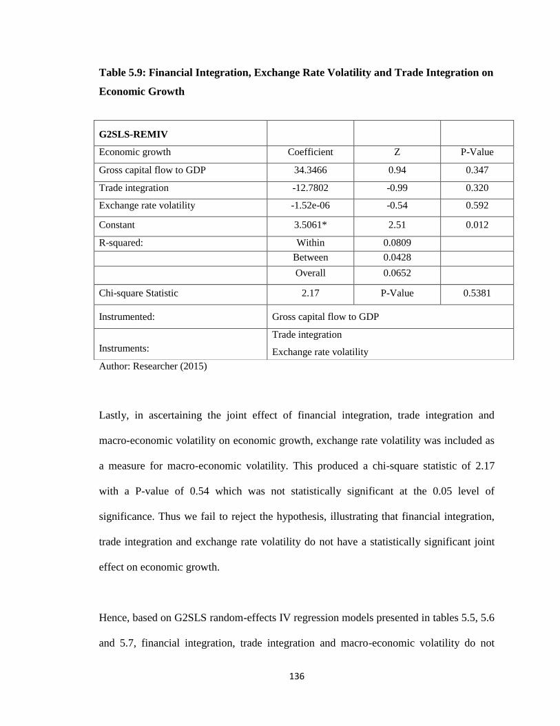
136

Table 5.9: Financial Integration, Exchange Rate Volatility and Trade Integration on

Economic Growth

Author: Researcher (2015)

Lastly, in ascertaining the joint effect of financial integration, trade integration and

macro-economic volatility on economic growth, exchange rate volatility was included as

a measure for macro-economic volatility. This produced a chi-square statistic of 2.17

with a P-value of 0.54 which was not statistically significant at the 0.05 level of

significance. Thus we fail to reject the hypothesis, illustrating that financial integration,

trade integration and exchange rate volatility do not have a statistically significant joint

effect on economic growth.

Hence, based on G2SLS random-effects IV regression models presented in tables 5.5, 5.6

and 5.7, financial integration, trade integration and macro-economic volatility do not

G2SLS-REMIV

Economic growth Coefficient Z P-Value

Gross capital flow to GDP 34.3466 0.94 0.347

Trade integration -12.7802 -0.99 0.320

Exchange rate volatility -1.52e-06 -0.54 0.592

Constant 3.5061* 2.51 0.012

R-squared: Within 0.0809

Between 0.0428

Overall 0.0652

Chi-square Statistic 2.17 P-Value 0.5381

Instrumented: Gross capital flow to GDP

Instruments:

Trade integration

Exchange rate volatility

137

have a statistically significant joint effect on economic growth. This being the main

research gap for this study, there was no comparable study from the literature reviewed.

The R2 values indicate that, 8.09% of the variations in economic growth, as measured by

GDP per capita, within the countries are explained jointly by financial integration,

exchange volatility and trade integration, 4.28% of the variations in economic growth

between the countries are explained jointly by financial integration, exchange rate

volatility and trade integration while 6.52% of the variations in economic growth of the

East African community as an economic bloc (considering panel data) are explained

jointly by financial integration, exchange rate volatility and trade integration. The above

results imply that, financial integration, exchange rate volatility and trade integration

cannot jointly be used to predict (relied upon) the level of economic growth.

According to Brada and Mendez (1988) integration is assumed to raise investment and

reduce risks. This can be explained by the fact that, a larger market will raise the

expected return on investments and reduce uncertainty by enabling firms to lower their

costs as a result of increased economies of scale, and a bigger pool of consumers. This

argument, captured under the new economic integration theory, is not supported by the

findings of hypothesis four in this study. This implies that, the East African economic

bloc is not a large enough market (it has low openness to trade and investment) to enjoy

the economies of scale of lowering transaction costs, hence reduce uncertainty. This is

explained by the low gross capital flows. The low integration levels can therefore be said

to contribute to the high macro-economic volatility.

138

5.3 Comparison between Expected Relationships and Actual Findings

Based on existing literature, it was expected that financial integration of the East African

community will have a positive significant effect on the growth of the economy so is the

case for trade integration. The findings do not correctly support this expectation.

Additionally, the findings were expected to depict negative significant influence of

macro-economic volatility on the relationship between financial integration and

economic growth. The lack of influence (no moderating effect) of GDP per capita

volatility, inflation volatility and exchange rate volatility on the relationship between

financial integration and economic growth from the findings deviates from this

expectation.

The researcher interprets this finding as a surprise because of the deviation of the actual

results from the expected results. The deviation calls for further probing into the

influence of macro-economic volatility on the relationship between financial integration

and economic growth, using a different set of measures of macro-economic volatility.

Trade integration was expected to have an intervening effect on the relationship between

financial integration and economic growth. The findings deviated from this expectation,

indicating the absence of intervening effect. Further, the joint effect of financial

integration, trade integration and macro-economic volatility on economic growth was

expected to be positive and significant. The findings do not support this expectation,

since financial integration, trade integration and macro-economic volatility do not have a

significant joint effect on economic growth.

139

The summary below on the hypotheses tests conducted above, indicates that, all the

findings support the hypotheses. This is so, because the hypotheses were stated in null

form.

Table 5.10: Summary of Hypotheses Results

Objective Hypotheses Findings

1 Fail to Reject Support

2 Fail to Reject Support

3 Fail to Reject Support

4 Fail to Reject Support

Source: Researcher (2015)

140

CHAPTER SIX

SUMMARY OF FINDINGS, CONCLUSION AND

RECOMMENDATIONS

6.1 Introduction

This chapter presents a summary of findings from correlation analysis and for each

research hypothesis, conclusion from these findings, study recommendations and the

contributions of the study. The chapter also identifies the limitations of the study and

future research directions.

6.2 Summary of Findings

Correlation analysis was conducted between financial integration and economic growth,

the various macro-economic volatility measures and economic growth, financial

deepening and financial integration, trade integration and financial integration, trade

integration and economic growth, macro-economic volatility and financial integration as

well as trade integration and macro-economic volatility. Respectively, the established

relationships on each of the set objectives were also summarized based on the inferential

statistical findings of regression analysis. The details are provided below.

Correlation analysis on the various variables indicated that, Gross capital flow to GDP

(financial integration) is positively and significantly correlated to economic growth.

GDP per capita volatility and exchange rate volatility were positively correlated to

economic growth though not statistically significant. However, inflation volatility was

negatively correlated to economic growth even though not statistically significant. The

141

two measures of financial deepening, namely, ratio of M2 to GDP and private bank credit

to GDP are positively and significantly correlated to financial integration.

Total exports and imports to GDP is positively and statistically significantly related to

financial integration. All the three measures for macroeconomic volatility were

positively correlated to financial openness, although only GDP per capita volatility and

exchange rate volatility had correlation values which were statistically different from 0

and ( r =0.4114, p < 0.05). GDP per capita volatility and exchange rate volatility were

positively and significantly correlated to trade integration.

In determining the relationship between financial integration and economic growth,

hypothesis one was tested. The results of testing the hypothesis indicate that, financial

integration as measured by gross capital flow to GDP is positively associated with

economic growth, though it does not have a significant effect on economic growth. The

results imply that, the presence of financial integration in an economy leads to improved

economic growth. Therefore, the East African community member states should put more

efforts on increasing the capital flows between the member states. This can be achieved

by tapping in more investments (capital investments by the governments, foreign direct

investments, investments in startup businesses, mutual fund flows with a focus on

increasing the net cash additions, the traditional asset classes of cash, stocks and bonds)

and trade flows.

142

In determining the moderating effect of Macro-economic volatility on the relationship

between financial integration and economic growth, the researcher tested hypothesis two.

Three indicators of macroeconomic volatility were separately applied in testing this

hypothesis. The results show that, the interaction term was not statistically significant in

all the models, indicating that each of the three measures of macroeconomic volatility has

no moderation effect on the relationship between gross capital flow to GDP and

economic growth. The implication of these findings is that, macro-economic volatility

does not play a role in determining the degree/strength of the relationship between

financial integration and economic growth.

Hypothesis three was tested to establish the intervening effect of trade integration on the

relationship between financial integration and economic growth. The results of testing

this hypothesis indicated that, the mediation term was not statistically significant in the

model. This means that, trade integration has no intervening effect on the relationship

between gross capital flow to GDP and economic growth. Therefore, the relationship

between financial integration and economic growth is not explained by the presence of

trade integration.

Hypothesis four was tested to establish the joint effect of financial integration,

macroeconomic volatility and trade integration on economic growth. Three measures of

macro-economic volatility were applied in testing this hypothesis, namely, GDP per

capita volatility, inflation volatility and exchange rate volatility. Using GDP per capita

volatility as a measure of macro-economic volatility, the results showed that, financial

143

integration, macroeconomic volatility and trade integration do not have a joint effect on

economic growth. The results implied that, financial integration, GDP per capita

volatility and trade integration cannot jointly be used to predict (relied upon) the level of

economic growth.

Based on exchange rate volatility as a measure of macro-economic volatility, the results

indicated that, financial integration, trade integration and exchange rate volatility do not

have a statistically significant joint effect on economic growth. The results implied that,

financial integration, exchange rate volatility and trade integration cannot jointly be used

to predict (relied upon) the level of economic growth. Using inflation volatility as a

measure of macro-economic volatility, the results illustrated that financial integration,

trade integration and inflation volatility do not have a statistically significant joint effect

on economic growth. The above results imply that, financial integration, inflation

volatility and trade integration cannot jointly be used to predict (relied upon) the level of

economic growth.

6.3 Conclusion of the Study

This study set out to determine the influence of macro-economic volatility and trade

integration on the relationship between financial integration and economic growth. The

failure to reject hypothesis one indicates that, financial integration as measured by gross

capital flow to GDP is positively associated with economic growth, though it does not

have a significant effect on economic growth. This leads to the conclusion that, countries

with low levels of gross capital flows are associated with low levels of economic growth

144

compared to the countries with relatively higher levels of gross capital flows. This

indicates that, increased economic growth is associated to increased/presence of financial

integration. This means that, countries experiencing an increase in gross capital flows are

likely to experience increase in gross domestic productivity.

On the first scenario of hypothesis two, looking at the effect of GDP per capita volatility

on economic growth, we fail to reject the hypothesis, indicating that, GDP per capita

volatility has no significant influence on the relationship between financial integration

and economic growth. We could therefore conclude that, when GDP per capita declines

or increases from a given level to a new level, the relationship between financial

integration and economic growth remains the same. In other words, GDP per capita

volatility does not have a moderating effect on the relationship between financial

integration and economic growth. On the second scenario, looking at the influence of

exchange rate volatility on the relationship between financial integration and economic

growth, we also fail to reject the hypothesis, indicating that, exchange rate volatility has

no significant effect on the relationship between financial integration and economic

growth. On the third scenario, we also fail to reject the null hypothesis that, inflation

volatility does not have a statistically significant effect on the relationship between

financial integration and economic growth. The study concludes that, inflation volatility

does not have an effect on the relationship between financial integration and economic

growth. Overall, the presence of macro-economic volatility in the EAC economic bloc

does not strengthen, weaken or reverse the relationship between financial integration and

economic growth.

145

The failure to reject hypothesis three indicates that, trade integration does not have an

intervening effect on the relationship between financial integration and economic growth.

We conclude that, trade flows do not impact on the relationship between capital flows

and economic growth. Therefore, the presence of trade flows does not explain the

relationship between capital flows and economic growth.

Three scenarios on hypothesis four in line with the three indicators of macro-economic

volatility used in this study, were presented. On the first scenario, exploring the joint

effect of financial integration, GDP per capita volatility and trade integration on

economic growth, the results showed that, financial integration, GDP per capita volatility

and trade integration do not have a joint effect on economic growth. On the second

scenario, the results showed that financial integration, exchange rate volatility and trade

integration do not have a joint effect on economic growth. On the third scenario, the

results showed that, financial integration, inflation volatility and trade integration do not

have a joint effect on economic growth. From all the three scenarios above, the study

concludes that, jointly, financial integration, macro-economic volatility and trade

integration have no effect on economic growth.

From the above specific conclusions, it can be generalized that, macro-economic

volatility and trade integration have no influence on the relationship between financial

integration and economic growth. However, at an individual level, there exists co-

movement between economic growth and each of the explanatory variables; financial

integration, macro-economic volatility and trade integration.

146

6.4 Recommendations of the study

The findings of this study are useful to the central banks of the respective East African

community member states as well as investors. The positive association between

financial integration and economic growth serves to benefit the member states through

their respective central banks which are mandated to manage the monetary policy. The

control of money supply as measured by M2 should be enhanced by adopting

expansionary monetary policy measures in an effort to increase its ratio to GDP. In trying

to expand money supply, the central banks could consider lowering the respective

countries‘ reserve ratios, so that the commercial banks have a wider deposit base which

enhances the creation of credit money.

They could also consider lowering the discount window which supports increased

lending capacity. More importantly, it is advisable for the banking sector to consider

increasing lending to the private sector. An effective way to achieve this would be for the

respective central banks to put limits on public borrowing from the domestic financial

markets (discourage aggressive selling of government securities). By extension, they can

consider putting measures in place to enhance government revenue collection, to meet the

budgetary needs. The respective governments could also consider exploring the various

sources of money supply and try to enhance them. Key sources of money supply would

be individual and corporate savings. Therefore, the East African governments should

continue to encourage both individuals and corporates to save more. Innovative products

for savings that are all-inclusive (accommodate all classes of East African citizens)

should be introduced across the East African region to encourage the savings effort.

147

Since the rise in food and fuel prices which has led to higher import bills and significant

balance of payment gaps is said to contribute to high volatility of currencies in net

importing countries such as Kenya, Tanzania and Uganda, we recommend that, the

respective governments work on a monetary policy that aims to attain a single digit level

of inflation rate (low inflation targeting), in the spirit of macro-economic convergence.

The diversity of the economic structures of the EAC countries in terms of incomes,

industrial structures and social indicators has been blamed for the slow progress in

achieving the monetary union as indicated in the discussion of the findings of hypothesis

three. It is therefore necessary for the respective member states to work towards making

their economic structures as similar as possible. This will help accelerate the pace of

integration, particularly, becoming a monetary union.

The findings of hypothesis one reveal that, the quality of institutions, development of the

financial markets, exchange rate volatility and inflation volatility are some of the key

determinants of the composition of capital flows. Since the finance sector development

which is largely viewed through the level of financial markets development, remains key

to economic growth, it is important for the member states to take more initiatives for

developing the financial markets, whose depth remains low, both in terms of product

portfolio and investor base. One of the initiatives is to remove the limit on foreign

investor ownership of listed firms and lower the transaction costs, especially the

brokerage fee on stock transactions. More incentives, in addition to the existing tax

incentives should be introduced to encourage more listings across the different sectors of

148

the economy. This is useful in widening the securities basket and hence enhance the room

for diversification of the risk of investing in stocks, as one of the traditional asset classes.

One of the measures of the quality of institutions is political stability which remains

elusive, going by the existing history. There is therefore the need to continue

implementing more political reforms, as part of the effort to improve the political

environment and ultimately stabilize it.

6.5 Contributions of the Study

The findings from this study contribute to the body of knowledge in the area of financial

integration, macro-economic volatility, trade integration and economic performance.

This section highlights the study findings contribution to knowledge.

The results of this study add to existing knowledge in the area of financial integration,

macro-economic volatility, trade integration and economic performance. The first major

contribution is the understanding of the association between the various variables on

which the study is based. On the primary relationship between financial integration and

economic growth, Gross capital flow to GDP (financial integration) depicted positive and

significant correlation to economic growth. This confirms that, an increase in gross

capital flows is accompanied by increase in economic growth.

GDP per capita volatility and exchange rate volatility were positively correlated to

economic growth though not statistically significant. Inflation volatility was negatively

correlated to economic growth even though not statistically significant. The two measures

149

of financial deepening, namely, ratio of M2 to GDP and private bank credit to GDP are

positively and significantly correlated to financial integration. This means that, financial

deepening contributes positively to financial integration which further contributes to

accelerating economic growth. This relationship confirms the economic theory that,

money supply controls economic growth.

6.6 Limitations of the Study

There are various challenges that were encountered in the conduct of this study, as a

result of the nature of the study, method of analysis, type of data, context as well as time

frame. The study was quantitative in nature, narrowing the researcher to focus on only

measures that are quantifiable yet a qualitative study or a combination of both would

have provided a wider array of variables to be studied, making the research more robust

and less biased. A similar challenge was posed by the type of data used. The study

applied secondary data only, limiting the degree of the accuracy of the study findings to

the accuracy of the data. This explains why reliability and validity tests were not carried

out but the researcher used credible sources such as World Bank and IMF to collect the

data, in an effort to ensure that, the findings are reasonably reliable.

This study was limited to the East African community as the context, a region that is too

small on the global map or even continent wise. Therefore, the findings are basically

applicable to the region and can only be relevant on the global map as a foundation for

similar but more extensive studies. A bigger context of the study and use of primary data

through interviews or questionnaires which captures more information and attributes of

150

different variables would have only been achievable with more financial resources and

investing more time on the research.

The consideration of the period 1963-2014, is faced with the limitation of missing data

points, as a result of economic stagnation occasioned by war in some of the member

states, although this limitation was taken care of by using balanced panel data. The study

was also faced by the limitation of using gross capital flows and trade flows from the

formal economy only, leaving out the capital flows from the informal economy,

especially the trade flows through the porous border of Somalia into Kenya. The trade

flows from the porous borders could be significant enough to impact on the economy and

so are the findings of this study.

6.7 Suggestions for further research

The conduct of this study has generated some research gaps which can be filled by

further studies in the future. First, the context of this study was the East African

community over the period 1963-2014, as a continuous duration. Conducting a

comparative study between the old and the new EAC may be necessary in establishing

whether the inclusion of Rwanda and Burundi, has had any positive impact (catalyzed) on

the level of financial integration and economic growth or even reduced macro-economic

volatility. Future research could focus on the African union as an economic bloc which

has a bigger mandate than the East African community. Africa as an economic bloc is

much more significant on the global economy than the East African community, which is

a small segment of the continent.

151

Therefore, focus on enhancing economic integration and economic growth of Africa as

an economic bloc is likely to lead to more synergistic benefits to individual countries than

the benefits arising from regional integration. A comparative study on the various

economic blocs such as ECOWAS and SADC currently existing in Africa is a

worthwhile consideration, as well. Such a study is likely to provide useful insights to

international investors on which African regions would be top priority areas as

investment destinations, based on the established inter-relationships between the four

variables analyzed in the current study.

The current study used defacto measures of financial integration and more specifically,

gross capital flows. Future studies can apply different indicators of financial integration

as well as macro-economic variables and possibly consider using de jure measures of

financial integration. Additionally, the use of qualitative data is recommended for

purposes of comparing the findings.

Future research could consider measuring the level of capital flows from the informal

economy and combine it with the capital flows from the formal economy to arrive at the

accurate aggregate value of gross capitals in the economy. The use of such an aggregate

value has the likelihood of altering the findings of the current study.

152

REFERENCES

Adam, K., Jappelli T., Menichin`i A. M., Padula M., and M. Pagano (2002). Analyse,

Compare, and Apply Alternative Indicators and Monitoring Methodologies to

Measure the Evolution of Capital Market Integration in the European Union,

Report to the European Commission.

Adler, M. and B. Dumas, (1983). International Portfolio Selection and Corporation

Finance: A Syn-thesis. Journal of Finance, 46, 925-984.

Afonso, A., and D. Furceri (2010). Government size, composition, volatility and economic

growth, European Journal of Political Economy, 26(4) 517-532.

Aghion, Banerjee and Piketty, (1999). Dualism and Macroeconomic Volatility, Quarterly

Journal of Economics 114, 1359–1397.

Aguiar, A., and G. Gopinath, (2007). Emerging Market Business Cycles: The Cycle Is

the Trend, Journal of Political Economy, University of Chicago Press, 115, 69-

102.

Alfaro, Laura, Sebnem Kalemi-Ozcan, and Vadym Volosovych, (2003). ―Why Doesn‘t

Capital Flow from Rich to Poor Countries? An Empirical Investigation,‖ Working

Paper 040 (Boston, Mass.: Harvard Business School).

Alfaro, Chanda, Kalemli-Ozcan, and Sayek, (2004). FDI and Economic Growth: The

Role of Local Financial Markets, Journal of International Economics, 64(1), 113-

34.

Allen. R. L. (1963). Review of The theory of economic integration, Economic

Development and Cultural Change 11(4), 449-454.

Allen, F. Brealey, R. Myers, S. (2011). Principles of Corporate Finance. New York:

McGraw-Hill/ Irwin.

American Statistical Association (1998). Ethical Guidelines for Statistical Practice.

153

Amor, T. H. & Sarkar, A. U. (2008). Financial integration and real exchange rate

volatility: Evidence from South and South East Asia, International Journal of

Business and Management 3(1): 112.

Arteta, C., B. Eichengreen and C. Wyplosz (2001). When Does Capital Account

Liberalization Help More than it Hurts?, NBER Working Paper, No. 8414.

Asiedu, Elizabeth, (2002). ―On the Determinants of Foreign Direct Investment to

Developing Countries: Is Africa Different?‖ World Development, 30 (January),

107-19.

Azeinman, J., and B. Pinto (2005). Overview in J. Azeinmanet B. Pinto, eds. Managing

Economic volatility and Crises. Cambridge, Mass.: Cambridge University Press.

Baele, L., A. Ferrando, P. Hordahl, E. Krylova and C. Monnet (2004). Measuring

Financial Integration in the Euro Area, Occasional Paper No.14, European

Central Bank, April.

Babietskii, I., Komárek, l., Komárková, Z. (2007). Financial Integration of Stock Markets

among New EU Member States and the Euro Area. CNB Working Paper Series,

No. 7.

Baker, S.R., Bloom, N., Davis, S. J., and Reenen, J. (2011). Economic Recovery and

Policy Uncertainty. CEP US Analysis Papers 002.

Balassa, B. (1961). The Theory of Economic Integration. Homewood, Illinois: Richard

D. Irwin.

Balcerowicz L., (2001). Libertateşidezvoltare. Economiapieţeilibere, Multiprint

Publishing House, Iasi.

Baldwin, Richard; Wyplosz, Charles (2004). The Economics of European Integration.

New York: McGraw Hill. ISBN 0-07-710394-7.

154

Barro, R. (2001). Economic Growth in Fast Asia before and After the Financial Crisis,

NBER Working Paper No 8330 (Cambridge, Massachusetts: National Bureau of

Economic Research).

Battalio, H., Mendenhall, R. (2005). Earnings expectation, investor trade size, and

anomalous returns around Earnings announcements. Journal of Financial

Economics, 77(2) 289–319.

Bates, R. H. (2005). Political Insecurity and State Failure in Contemporary Africa, CID

Working Paper, 115, Harvard University.

Baxter and Crucini, (1995). Business cycles and the asset structure of foreign trade,

International Economic Review 36, 821–854.

Bekaert, Geert, Campbell R. H. and Lundblad. C, (2001). Emerging Equity Markets and

Economic Development, Journal of Development Economics, 66 465–504.

Bekaert, Harvey, Lundblad, (2001). Growth Volatility and Equity Market Liberalization.

Working Paper. Duke University.

Bekaert, Harvey, Lundblad, (2002). Does Financial Liberalization Spur Growth? Mimeo,

Columbia University.

Black, F. (1974). International capital market equilibrium with investment barriers.

Journal of Financial Economics, 1, 337-352.

Blanchard, O. and Simon, J. (2001). The Long and Large Decline in US, Brookings Papers

on Economic Activity.

Blomstrom M., R. E. Lipsey, M. Zejan (1994). What Explains Developing Countries

Growth?, NBER Working Paper, No. 4132. Bloom, D. and Sachs, J.

(1998).Geography, demography, and Economic Growth in Africa Brookings

Papers of Economic Activity, 2,207-73.

155

Blumberg, B., Cooper, D. R. & Schindler, P.S. (2005). Business research methods.

London: The McGraw-Hill Companies.

Blume, L. Durlauf, S. (2008). The New Palgrave Dictionary of Economics. New York:

Palgrave Macmillan.

Bonfiglioli, A. (2008). Financial Integration, Productivity and Capital Accumulation,

Journal of International Economics, 76:337-55.Borensztein, Eduardo, José De

Gregorio, and Jong-Wha Lee, 1998, How Does Foreign Direct Investment Affect

Growth? Journal of International Economics, 45, 115–35.

Borensztein, Eduardo, Jose de Gregorio, and Jong-wha Lee, 1998, ―How does foreign

Investment Affect Growth?‖ Journal of International Economics, 45 (June), 115-

135.

Bouman, S. & Jacobsen. B. (2002). The Halloween Indicator, Sell in May and Go Away:

Another Puz- zle. American Economic Review, 92(5) 1618–1635.

Boyd, J. H. & Smith. B. D. (1992). Intermediation and the Equilibrium Allocation of

Investment Capital: Implications for Economic Development, Journal of

Monetary Economics, 30(1), and 409-32.

Brada, Joseph C., & Mendez. J. A. (1988). An estimate of the dynamic effects of

economic integration. The Review of Economics and Statistics 70(1), 163-168.

Brouwer, G. (2005). Monetary and Financial Integration in Asia: Empirical Evidence and

Issues, in Asia Economic Cooperation and Integration, Manila: Asia Development

Bank.

Bryman, A. & Bell, E. (2007). Business Research Methods, 2nd

edition. Oxford University

Press.

Buch, Dopke, Pierdzioch, (2002). Financial openness and business cycle volatility,

Working Paper, Kiel Institute for World Economics.

156

Buigut, S. (2011). A Fast-Track East African Community Monetary Union? Convergence

Evidence from A Cointegration Analysis, International Journal of Economics and

Finance, Vol. 3, No. 1; Burnside, C. and Dollar, D. (2000).Aid, Policies and

Growth American Economic Review, 90(4), 847- 868.

Calderόn, C., & Liu, L. (2003). The direction of causality between financial development

and economic growth. Journal of Development Economics, 72, 321-334.

Caporale, G., Amor, T. & Rault, C. (2009). Sources of real exchange rate volatility and

international financial integration: A dynamic gmm panel data approach, Brunel

University West London, Working Paper Number 09-21.

Cappiello, L., Gérard, B. Kadareja, A. and Manganelli, S. (2006). Financial Integration of

new EU Member States, European Central Bank Working Paper No. 68.

Caprio, Gerard, and Honohan.P, (1999). "Restoring Banking Stability: Beyond

Supervised Capital Requirements," Journal of Economic Perspectives, 13(3), 43-

64.

Cassel, Gustav (1918). Abnormal Deviations in International Exchanges. 28, 112 (112).

The Economic Journal. 413–415.

Cheung Y, M.D. Chinn, E. Fujii (2003). China, Hong Kong, and Taiwan: A quantitative

assessment of real and financial integration, China Economic Review 14, 281–

303.

Chowdhury, A. R. (2001). Foreign Debt and Growth in Developing Countries: A

Sensitivity and Causality Analysis Using Panel data.

Collier, P. and O‘Connell, A. (2004). Explaining Africa Economic Growth: Opportunities

and Choices, AERC Growth Project Synthesis, Draft Chapter 2, August.

Collis, J., & Hussey, R. (2003). Business research – a practical guide for undergraduate

and postgraduate Students (2nd

ed.). Palgrave Macmillan: Great Britain. Denizer,

C., Iyigun, A.,

157

Combes, J.L., and P. Guillaumont. (2002). Commodity Price Volatility, Vulnerability and

Development. Development Policy Review.

Cooper, I. and E, Kaplanis, (2000). Partially Segmented International Capital Markets

and International Capital Budgeting. Journal of International Money and

Finance, 43(1), 287-307.

Cooper, C. A., and B. F. Masselll. (1965a). A new look at customs union theory. The

Economic Journal 75(300), 742-747.

De Gregorio, J., & Guidotti, P.E. (1995). Financial development and economic growth.

World Development, 23(4), 433-448.

Dumas, B. and B, Solnik. (1995). The World Price of Foreign Exchange Risk. Journal

of Finance, 50(9) 445-479.

EAC (2011), EAC Development Strategy (2011/12–2015/16), Deepening and

Accelerating Integration.

Eakins, G., Mishkin, S. (2012). Financial Markets and Institutions. Boston: Prentice Hall.

Easterly, W., Kremer, M., Pritchett, L. and L. H. Summers (1993). Good policy or good

luck?: Country growth performance and temporary shocks. Journal of Monetary

Economics .32(3), 459-483.

Easterly, W. Islam, R. Stiglitz, J., (2001). Shaken and stirred: Explaining Growth

Volatility.

Edison, H., Levine, R., Luca R., Sløk, T., (2002). International Financial Integration and

Economic Growth. Journal of International Monetary and Finance 21749-7624.

Eichengreen, B. J., (2001). ―Capital Account Liberalization: What Do the Cross-Country

Studies Tell Us?‖ World Bank Economic Review, 15(4),341–66.

Elly. D. O. (2014).Effects of market geography and institutional quality on financial

markets integration in the East African community. Published PhD thesis.

158

Errunza, V. and E, Losq. (1985). International Asset Pricing Under Mild Segmentation:

Theory and Test. Journal of Finance, 40(6), 105-124.

Eun, C. S. and S, Janakiramanan. (1986). A Model of International Asset Pricing with a

Constraint on the Foreign Equity Ownership. Journal of Finance, 41(6), 897-914.

Fama, E., (1970). Efficient Capital Markets: A Review of Theory and Empirical Work,

Journal of Finance. 25(2), 383 –417.

Fama, E. F., & French, K. R. (1988).Permanent and temporary components of stock

prices.Journal of Political Economy, 96(2), 246-273.

Fatás, A., (2002). The Effects of Business Cycles on Growth, in Economic Growth:

Sources, Trends and Cycles. Eds. Loayza, N., and Soto, R., Central Bank of

Chile.

Fatás, A, and I. Mihov (2005). Policy Volatility, Institutions and Economic Growth.

Working Paper 5388, Centre for Economic Policy Research.

Fatas, A, and I. Mihov (2007). Fiscal Discipline, Volatility, and Growth, in Fiscal Policy,

Stabilization, and Growth , eds. Perry G., Servén, L., and R. Suescun, Latin

American Development Forum, The World Bank.

Foroutan, Faezeh and Pritchett. L (1993). Intra-Sub-Saharan African Trade: is it too

Little? Journal of African Economies, 2(1),74-105.

Garibaldi, Pietro, and others, (2002). ―What Moves Capital to Transition Economies,‖

IMF Working Paper 02/64 (Washington: International Monetary Fund).

Gavin, Michael, and Ricardo Hausmann, (1996). Sources of Macroeconomic Volatility in

Developing Economies, Working Paper, Inter-American Development Bank.

Giannetti, Mariassunta, Guiso. L, Jappelli. T, Padula. M and Pagano. M, (2002).

‗Financial Market Integration, Corporate Financing and Economic Growth: Final

Report‘, European Economy Economic Papers, No. 179, Brussels.

159

Goedhart, M., Koller, T., Wessels, D. (2010). Valuation New Jersey: John Wiley & Sons

Goldberg, Linda, and Charles Kolstad, (1994). ―Foreign Direct Investment, Exchange

Rate Variability, and Demand Uncertainty,‖ NBER Working Paper No. 4815

(Cambridge, Massachusetts: National Bureau of Economic Research).

Goldberg, L. (2004). Financial-Sector FDI and Host Countries: New and Old Lessons,

NBER Working Paper No. 10441 (Cambridge, Massachusetts: National Bureau of

Economic Research).

Gomez-Haro, S., Aragon-Correa, J., and Cordon-Pozo,. E. (2011). Differentiating the

effects of the institutional environment on corporate entrepreneurship.

Management Decision, 49(10), 1677-1693.

Goodhart, C. (1998). The two concepts of money: implications for the analysis of

optimal currency areas, European Journal of Political Economy14 (3): 407–432.

Gourinchas, Pierre-Olivier, and Olivier. J, (2003). The Elusive Gains from International

Financial Integration, NBER Working Paper 9684.

Guiso, L., Jappelli, T., Padulla, M., & Pagano, M. (2004). Financial market integration

and economic growth in the EU. Economic Policy, 19(5), 523-577.

Grier, K., Tullock, G., (1989). An Empirical Analysis of Cross-National Economic

Growth, 1951–80, Journal of Monetary Economics 24(1989), 259–276.

Grossman, Sanford J and Oliver D. H. (1986). The Costs and Benefits of Ownership: A

Theory of Vertical and Lateral Integration. Journal of Political Economy 94(4),

691–719.

Hau, H. (2002). Real exchange rate volatility and economic openness: theory and

evidence, Journal of money, Credit and Banking pp. 611630

Hayek F. A. (1899-1992). The Concise Encyclopedia of Economics Library of Economics

and Liberty. Econlib.org. Retrieved 2012-05-1.

160

Hayek. F. A. (1974). Denationalization of Money: The Argument Refined, Mises.org.

Retrieved 2012-10-07.

Heathcote, J. & Perri, F. (2004). The international diversification puzzle is not as bad as

you think, Meeting Papers 152, Society for Economic Dynamics.

Heather, M.E., Porter, T. and Roberge, I. (2004).Politics or Markets? The determinants

of cross integration in the NAFTA and the EU, New Political Economy, 9(3), 325-

340.

Henry, Peter, (2000). Do Stock Market Liberalization Cause Investment Booms? Journal

of Financial Economics, 58(5), 301–34.

Hnatkovska, V., Loayza, N., (2003).Volatility and Growth. Working Paper, World Bank.

Ho, N.W. (2009). Financial Integration: Concepts and Impacts, Macao Monetary

Research Bulletin, 10, 69-84.

International Monetary Fund (2001). World Economic Outlook, October, World

Economic and Financial Surveys (International Monetary Fund, Washington).

Jappelli, T. and Pagano, M. (2008). Financial Market Integration under EMU‟, CEPR

Discussion Paper No. 709.

Jayaratne J. and Strahan, P. (1996). The Finance-Growth Nexus: Evidence from Bank

Branch Deregulation, Quarterly Journal of Economics, 111,639-70.

Jeanne, O. (2003). Why Do Emerging Market Economies Borrow in Foreign Currency?

IMF Working Paper 03/177, Washington, DC.

Jetter, M. (2014). Volatility and Growth: Governments are Key. European Journal of

Political Economy, 36: 71 – 88.

Joshua S. Goldstein (2005). International Relations, New York: Pearson-Longman.

161

Kaijage, E. S. and Nzioka, O. M. (2012). Determining the Extent of Financial Integration

in East Africa Using Beta Convergence and Co-integration Analysis. ORSEA

Journal, Volume 2.

Kaiser, P. J. (1996). Structural Adjustment and the Fragile Nation: The Demise of Social

Unity in Tanzania. The Journal of Modern African Studies. 34(2), 227–237.

Kalemli-Ozcan, S. and Manganelli, S. (2008). Financial Integration and Risk Sharing:

The Role of the Monetary Union, in 5th

European Central Banking Conference on

The Euro at Ten: Lessons and Challenges, Frankfurt: ECB.

Kalemli-Ozcan, S. Sorensen, B.Yosha, O., (2003). Risk Sharing and Industrial

Specialization: Regional and International Evidence, American Economic Review

93.

Kamaly, Ahmed, (2002). ―Behind the Surge in FDI to Developing Countries in the

1990s: An Empirical Investigation‖ (unpublished; College Park, Maryland:

University of Maryland).

Kaniel, R., Liu, S. Saar, G., Titman, S. (2012). Individual Investor Trading and Return

Patterns around Earnings Announcements. Journal of Finance, 67(2), 639–680.

Kenen, P. (1969). The Optimum Currency Area: An Eclectic View, In Mundell and

Swoboda, (eds.), Monetary Problems of the International Economy, Chicago:

University of Chicago Press.

Keohane, R. O. (1984). After Hegemony: Cooperation and Discord in the World Political

Economy. Princeton: Princeton University Press.

Keynes, J. M., A. Tract on Monetary Reform (London, 1923). A Treatise on Money, Vol.

I. (London, 1930).

Kindleberger. C. (1981). Dominance and Leadership in the International Economy, 25(2)

International Studies Quarterly 242-54.

162

Kindleberger, C. P., (1986). The World in Depression, 1929-1939. Berkeley: University

of California Press. King, Robert G and Ross Levine. (1993), Finance and

Growth: Schumpeter might be right. The Quarterly Journal of Economics.108 (3).

Kose, M. A. (2002). Explaining business cycles in small open economies, Journal of

International Economics, 56, 299–327.

Kose, M. Ayhan, Eswar S. Prasad, and Marco E. Terrones, (2003a), "Financial

Integration and Macroeconomic Volatility," IMF Staff Papers, 50 (Special Issue),

119-42.

Kose, M. A., Prasad, E., Terrones, M., (2003). Financial Integration and Macroeconomic

Volatility, IMF Staff Papers (Washington: International Monetary Fund), 50,

119–42.

Kose, M. A., Prasad, E., Terrones, M., (2004). Volatility and Movement in a Globalized

World Economy: An Exploration, forthcoming, in Horst Siebert ed.,

Macroeconomic Policies in the World Economy, Springer.

Kraay, A. (1998). In Search of the Macroeconomic Effects of Capital Account

Liberalization, Manuscript, the World Bank.

Kreinin, M. (1964). On the Dynamic Effects of a Customs Union. The Journal of

Political Economy 72(2), 193-195.

Krugman, P. (1991). The Move towards Free Trade Zones, in Policy Implications of Free

Trade and Currency Zones. A Symposium Sponsored by the Federal Reserve

Bank of Kansas City. Jackson Hole, Wyoming, August 1991.

Krugman P. (1993). Lessons from Massachusetts for EMU" in Torres, F. & Giavazzi, F.

(Editors) Adjustment and Growth in the European Monetary Union London:

CEPR and Cambridge University Press.

Lake, David. (1993). Leadership, Hegemony, and the International Economy:

International Studies Quarterly, 37:459-489.

163

Lake, David A. (2009). Open Economy Politics: A Critical Review. Review of

International Organizations 4(3), 219–244.

Lane P., R. (2000). International Investment Position: A Cross Sectional Analysis,

Journal of International Money and Finance, 19, 513–534.

Levine, R. (1997). Financial development and economic growth: views and agenda,

Journal of Economic Literature, 35,688-726.

Levine, R. (2001). International financial liberalization and economic growth, Review of

International Economic, 9: 688–702. Lucas, R. E. (1988). 'On the Mechanisms of

Economic Development, Journal of Monetary Economics, 22, 3-42.

Levin, J. (2001). Taxation in Tanzania. United Nations University World Institute for

Development Economic Research Discussion Paper No. 20001/80. Marat F. &

Ann, O. (2002).Finance and macroeconomic volatility. The B. E. Journal of

Macroeconomics 2 (1), Article 7.

Lin, S.C., and Kim, D. H. (2014). The Link between Economic Growth and Growth

Volatility. Journal of Empirical Economics, 46, 43 – 63.

Lyakurwa, William, Andres M., Ng‘eno. N. and Kennes. W. (1997). Regional Integration

in Sub-Saharan Africa: A Review of Experiences and Issues in Regional

Integration and Trade Liberalization in Sub-Saharan Africa, Volume I:

Framework, Issues and Methodological Perspectives. London: Macmillan.

Malkiel, B. G. (2011). The efficient-market hypothesis and the financial crisis.

Rethinking Finance: Perspectives on the Crisis (Proceedings of a Conference).

Russel Sage Foundation.

Marshall, A. (1890). Principles of Economics, 8th

edition 1920. Reprint, reset (1977),

London: Macmillan.

Marshall, A, (1930). Principles of Economics: An Introductory Volume. 8th

, London,

Macmillan.

164

Marshall, B., Visaltanachoti, N. (2010). The other January effect: evidence against

market efficiency? Journal of Banking & Finance, 34(10), 2413–2424.

Martin, P., Rogers, C., (2000). Long-term Growth and Short-term Economic Instability,

European Economic Review 44, 359-381.

McAuliffe, Catherine, Sweta .C, and Yabara. M, (2012), Journal of Monetary Economics

Prospects for Sustained Growth, IMF Working Paper No. 12/272.

McCarthy, J., and R. W. Peach. (2002). Monetary Policy Transmission to Residential

Investment. Federal Reserve Bank of New York Economic Policy Review 8(1)139-

58.

———. 2004. Housing Trends in the (1990s): The Effects on Rent Inflation and Its

Measurement in the CPI. Unpublished paper, Federal Reserve Bank of New York.

McKinnon, R. (1963). Optimum Currency Areas. American Economic Review, 52, 717-

725.

McConnell, M. and Perez-Quiros, G., (2000). Output °fluctuations in the United States;

What has changed since the early 1980s?, American Economic Review 90(5),

1464-1476.

Mendoza, E.G., (1995). The Terms of Trade, the Real Exchange Rate and Economic

Fluctuations, International Economic Review, 36, 101–137.

Miller, D. C., & Salkind, N. J. (2002). Handbook of Research Design & Social

Measurement. (6th

ed.). Thousand Oaks, CA: Sage.

Morisset, Jacques, (2000). Foreign Direct Investment in Africa: Policies Also Matter,

Policy Research Working Paper No. 2481, (Washington: The World Bank and the

International Finance Corporation).

165

Mougani, G. (2012). An Analysis of the Impact of Financial Integration on Economic

Activity and Macroeconomic Volatility in Africa within the Financial

Globalization Context, Working Paper Series No 144, African Development

Bank, Tunis, Tunisia.

Njoroge, L. (2010). The impact of regional integration on economic growth: empirical

evidence from COMESA, EAC and SADC trade blocs. American Journal of

Social and Management Sciences, 2010, 1(2), 150- 163.

Obstfeld, M. (1994). Risk-Taking, Global Diversification, and Growth, American

Economic Review, 84, 1310-29.

Obstfeld, M., and K. Rogoff, (1995), ―Exchange Rate Dynamics Redux‖, Journal of

Political Economy, 103, 624–60.

O‘Donnell, B., (2001). ―Financial Openness and Economic Performance‖ (Unpublished;

Dublin: Trinity College).

Opolot, J., & Luvanda, E. (2009). Macroeconomic Convergence in the East African

Community: Progress and Implications for the Proposed Union, Bank of Uganda

Staff papers, 53-79.

Osada, M. and Saito M. (2010). Financial Integration and Economic Growth: An

Empirical Analysis Using International Panel Data from 1974-2007. Research and

Statistics Department, Bank of Japan.

Olson, Mancur. (1965). The Logic of Collective Action. Cambridge: Harvard University

Press.

Palan, S. (2004). The efficient market hypothesis and its validity in today‘s markets.

Master thesis. Graz: Faculty of Social and Economic Sciences, Karl-Franzens

University, Graz.

Pigou, A. C., (1922). The Foreign Exchanges, Quarterly Journal of Economics, 37 1922).

166

Prasad, E., Rogoff, K., Wei, S., Kose, M., (2003). Effects of Financial Globalization on

Developing Countries: Some Empirical Evidence, IMF Occasional Paper No.

220(Washington: International Monetary Fund).

Quinn, D. (1977). The Correlates of Change in International Financial Regulation,

American Political Science Review, 91, 531-51.

R. A. Mundell, "The International Disequilibrium System," Kyklos, (1961) (2), 14, 153-

72.

Raddatz, C. (2007). Are external shocks responsible for the volatility of output in low-

income countries? Journal of Development Economics, 84(1), 155-187.

Rajmund and Aneta (2014). Financial Integration, Volatility of Financial Flows and

Macroeconomic Volatility, MPRA Paper No. 61845, Technical University in

Kosice, Slovak Republic.

Rajmund et al (2015). Relationship between Financial Integration, Financial

Liberalization and Macroeconomic Volatility, MPRA Paper No. 66143, Technical

University in Kosice, Slovak Republic.

Ramey, G., Ramey, V., (1995). Cross-Country Evidence on the Link between Volatility

and Growth, The American Economic Review, 85(5), 1138–1151.

Ranciere, R., A. Tornell and F. Westermann, (2008). Systemic Crises and Growth, The

Quarterly Journal of Economics, MIT Press, 123(1), 359-406.

Razin, Assaf and K. Rose. (1994). Growth, the Pro Capital Mobility: The Impact on

Consumption, Investment, and Growth, (Cambridge: Cambridge University

Press), 48-76.

Rector, Chad. (2009). Federations: The Political Dynamics of Cooperation. Ithaca:

Cornell University Press.

167

Reisen, Helmut, and Soto. M, (2001). Which Types of Capital Inflows Foster

Developing- Country Growth? International Finance, 4(1)1–14.

Rogoff, K., (1996). The Purchasing Power Parity Puzzle, Journal of Economic Literature

34: 647-668.

Rogoff, Kenneth, and Carmen Reinhart, (2003). ―FDI to Africa: The Role of Price

Stability and Currency Instability,‖ IMF Working Paper 03/10 (Washington:

International Monetary Fund).

Romer, C., (1986). Is the stabilization of the post-war economy argument of the data?

American Economic Review 76, 314 -334.

Saint-Paul, G. (1992). Technological choice, financial markets and economic

development, European Economic Review, 36:763-81.

Schafer, S. (2009). EU retail banking: Measuring integration, EU Monitor, 63, 1-16.

Schelling, T. (1978). Micromotives and Macrobehavior. New York, N.Y.: W.W. Norton.

Schiff, Maurice, and L. Alan W. (1998). Dynamics and politics in regional integration

arrangements: An introduction. The World Bank Economic Review 12(2), 177-

195.

Schwert, G. W. (2003). Anomalies and market efficiency. In Constantinides, G. M.,

Harris, M., and Stulz, R. M., editors, Handbook of the Economics of Finance:

Volume 1B, Financial Markets and Asset Pricing, volume 21 of Handbooks in

Economics, chapter 15, pp. 937-972. Elsevier North-Holland, Amsterdam.

Serven, L. (1997). Uncertainty, Volatility, and Irreversible Investment: Theory, Evidence,

and Lessons for Africa. Journal of African Economies, 6(3), 229-268.

Shiller, R. (2003). From efficient markets theory to behavioral finance. Journal of

Economic Perspectives, 17(1) 83–104.

168

Solnik, B. (1974). An Equilibrium Model of the International Capital Market. Journal of

Economic Theory, 8: 500-524.

Solow, R. (1956): ―A Contribution to the Theory of Economic Growth‖ Quarterly

Journal of Economics, 70(1): 65-74.

Stivers, C.Sun, L.Sun, Y. (2009). The other January effect: international, style, and sub-

period evidence. Journal of Financial Markets, 12(3), 521–546

Stulz, R. M. (1981). On the Effects of Barriers to International Investment. Journal of

Finance, 36, 923-934.

Stulz, R. (1999). ―Globalization of Equity Markets and the Cost of capital‖, NBER

Working Paper 7021 (March).

Tornell, Frank. W. and Lorenza M, (1998). The Positive Link Between Financial

Liberalization, Growth, and Crises, March 2004 USAID.

Trichet, J.C. (2005). Financial markets integration in Europe: the ECB‟s view, BIS

Review, 39: 1-5.

USAID Policy Paper Financial Markets Development Bureau for Program and Policy

Coordination U.S. Agency for International Development Washington DC.

Vajanne, L. (2006). Integration in Euro Area Retail Banking Markets - Convergence of

Credit Interest Rates. Bank of Finland Working Paper No. 8.

Vanek, J. (1962). International Trade: Theory and Economic Policy (Homewood, Illinois.

Viner, J. (1950). The Customs Union Issue. New York: Carnegie Endowment for

International Peace.

Walz, U. (1997). Dynamic Effects of Economic Integration: A Survey Open Economies

Review, 8(3), 309- 326.

169

Wang, Y. D., (2010). “Measuring Financial Barriers among East African Countries,”

IMF Working Paper 10/194, Washington: International Monetary Fund.

Williamson, Oliver E. (1985). The Economic Institutions of Capitalism: Firms, Markets,

Relational Contracting. New York: Free Press.

Wolf, H. (2005). Volatility: Definitions and Consequences. In J. Azeinman and B. Pinto,

eds. Managing Economic volatility and Crises. Cambridge, Mass.: Cambridge

University Press.

World Bank. World Development Report, (1989).

World Bank (2000). The Quality of Growth, (World Bank: Washington DC).

World Bank (2011a). Global Development Finance, Washington DC. Wray, L. Randall

(July 2000). "The Neo-Chartalist Approach to Money"(Working Paper No. 10).

Center for Full Employment and Price Stability.

www.worldbank.org.

170

APPENDICES

Appendix I: Raw Data C

ou

ntr

y

Co

de

yea

r

Eco

no

mic

gro

wth

: th

e

rate

of

chan

ge

of

rea

l

GD

P

GD

P,

bil

lio

ns

of

U.S

.

do

lla

rs

Infl

ati

on

: %

Ca

pit

al

inv

estm

ent/

GD

P

Ca

pit

al

inv

estm

ent,

bil

lion

US

D

Ex

cha

ng

e ra

te:

loca

l

curr

ency

un

its

per

U.S

.

do

lla

r

Ex

po

rts

of

go

od

s a

nd

serv

ices

, b

illi

on

US

D

Imp

ort

s o

f go

od

s a

nd

serv

ices

, b

illi

on

US

D

To

tal

Ex

po

rt a

nd

Imp

ort

s

( E

xp

ort

s a

nd

Imp

ort

s)/G

DP

Imp

ort

s/G

DP

Ex

po

rts/

GD

P

Fo

reig

n D

irec

t

Inv

estm

ent,

per

cen

t o

f

GD

P

Fo

reig

n D

irec

t

Inv

estm

ent,

bil

lio

n U

SD

Cu

rren

t a

cco

un

t b

ala

nce

as

per

cen

t o

f G

DP

Ba

nk

cre

dit

to

th

e

pri

va

te s

ecto

r/G

DP

Rea

l in

tere

st r

ate

M2

/GD

P

Burundi BI 1963 4.14 0.23

6.02 0.01 50 0.02 0.03 0.05 0.22 14.29 7.52

Burundi BI 1964 6.27 0.26

5.37 0.01 50 0.04 0.03 0.07 0.27 12.08 14.09

10.27804379

Burundi BI 1965 3.97 0.16

5.77 0.01 84.38 0.02 0.02 0.04 0.25 12.53 10.35

10.33901843

Burundi BI 1966 4.61 0.17 4.4 6.77 0.01 87.5 0.02 0.02 0.04 0.24 12.99 10.78

2.47

9.47058661

Burundi BI 1967 13.82 0.18 -1.1 6.85 0.01 87.5 0.02 0.02 0.04 0.22 11.89 10.8

2.66

10.49355811

Burundi BI 1968 -0.3 0.18 6.1 8.19 0.02 87.5 0.02 0.02 0.04 0.22 13.37 10.3

3.11

10.53212726

Burundi BI 1969 -1.46 0.19 4 8.29 0.02 87.5 0.02 0.02 0.04 0.21 12.09 9.66

2.73

10.54857898

Burundi BI 1970 21.33 0.24 -0.2 4.53 0.01 87.5 0.03 0.03 0.06 0.25 11.62 10.69

2.9

10.49761996

Burundi BI 1971 2.75 0.25 3.9 7.61 0.02 87.5 0.02 0.04 0.06 0.24 14.17 8.44

3.75

12.34965218

Burundi BI 1972 -6.4 0.25 3.8 3.18 0.01 87.5 0.03 0.04 0.07 0.28 15.07 11.73

4.42

12.39986293

Burundi BI 1973 6.89 0.3 6 5.31 0.02 80.03 0.03 0.04 0.07 0.23 13.33 11.02

4.36

12.86301432

Burundi BI 1974 -0.73 0.35 15.7 4.05 0.01 78.75 0.03 0.05 0.08 0.23 15.53 9.75

6.48

13.59421836

Burundi BI 1975 0.7 0.42 15.7 7.58 0.03 78.75 0.03 0.08 0.11 0.26 19 8.28

5.34

10.71979054

Burundi BI 1976 7.94 0.45 6.9 9.09 0.04 86.25 0.06 0.07 0.13 0.29 16.65 13.73

3.11

13.93746962

Burundi BI 1977 11.47 0.55 6.8 11.2 0.06 90 0.1 0.09 0.19 0.35 17.29 17.6

2.98

13.8867897

Burundi BI 1978 -0.94 0.61 23.9 14.04 0.09 90 0.07 0.12 0.19 0.31 20.23 11.71

4.13 -0.45 16.06855753

Burundi BI 1979 1.66 0.78 36.5 14.92 0.12 90 0.11 0.18 0.29 0.37 22.72 14.16

6.35 -11.2 13.54169773

Burundi BI 1980 0.99 0.92 2.5 13.89 0.13 90 0.08 0.21 0.29 0.32 23.29 8.81

6.13 -3.77 11.91320127

Burundi BI 1981 12.16 0.97 12.2 17.01 0.16 90 0.09 0.21 0.3 0.31 22.04 9.14

8.17 19.23 14.72684494

Burundi BI 1982 -1.05 1.01 5.9 14.46 0.15 90 0.1 0.27 0.37 0.37 26.91 10.21

8.56 5.99 13.36670688

Burundi BI 1983 3.72 1.08 8.2 22.83 0.25 92.95 0.1 0.27 0.37 0.34 24.75 9.05

7.19 5.23 15.72135349

Burundi BI 1984 0.16 0.99 14.3 18.37 0.18 119.71 0.11 0.23 0.34 0.34 23.55 11.5

5.04 -4.45 13.78671586

Burundi BI 1985 11.78 1.15 3.8 13.86 0.16 120.69 0.13 0.24 0.37 0.32 20.79 11.03 0.05 0

3.25 6.6 14.30337702

171

Burundi BI 1986 3.25 1.2 1.7 11.64 0.14 114.17 0.14 0.27 0.41 0.34 22.32 11.72 0.13 0

3.83 16.98 14.48859702

Burundi BI 1987 5.5 1.13 7.1 22.61 0.26 123.56 0.11 0.29 0.4 0.35 25.74 9.74 0.12 0

4.26 15.96 14.45952905

Burundi BI 1988 5.03 1.08 4.5 15.04 0.16 140.4 0.14 0.28 0.42 0.39 25.95 12.59 0.11 0

4.9 8.22 15.39186913

Burundi BI 1989 1.35 1.11 11.7 16.46 0.18 158.67 0.11 0.26 0.37 0.33 22.94 9.75 0.05 0

6.07 -2.4 15.73663455

Burundi BI 1990 3.5 1.13 7 14.54 0.16 171.26 0.09 0.31 0.4 0.35 27.78 7.87 0.11 0

7.26 6 15.77853083

Burundi BI 1991 5 1.17 9 14.41 0.17 181.51 0.12 0.33 0.45 0.38 28.51 9.92 0.08 0

9.46 8.35 17.03560203

Burundi BI 1992 1.01 1.08 1.8 10.64 0.12 208.3 0.09 0.32 0.41 0.38 29.48 8.75 0.06 0

10.05 7.83 16.90753577

Burundi BI 1993 -6.24 0.94 9.7 11.54 0.11 242.78 0.09 0.25 0.34 0.36 27.16 9.38 0.05 0

11.61 5.59 17.73312871

Burundi BI 1994 -3.83 0.93 14.9 6.97 0.06 252.66 0.1 0.26 0.36 0.39 28.48 10.27 0 0

12.16 7.09 23.00520667

Burundi BI 1995 -7.92 1 19.3 6.36 0.06 249.76 0.13 0.27 0.4 0.40 27.28 12.93 0.2 0

13.14 -0.73 19.80361436

Burundi BI 1996 -8 0.87 26.4 8.21 0.07 302.75 0.05 0.14 0.19 0.22 15.75 5.82 0 0

12.54

22.33230711

Burundi BI 1997 -1.59 0.97 31.1 6.1 0.06 352.35 0.1 0.14 0.24 0.25 14.44 9.84 0 0

11.15

18.5863769

Burundi BI 1998 4.75 0.89 12.5 6.77 0.06 447.77 0.07 0.17 0.24 0.27 19.44 8 0.22 0

11.67

15.78588206

Burundi BI 1999 -1.01 0.81 3.4 5.88 0.05 563.56 0.06 0.13 0.19 0.23 15.96 7.58 0.03 0

12.73 0.25 20.47373737

Burundi BI 2000 -0.86 0.87 24.3 2.78 0.02 720.67 0.06 0.14 0.2 0.23 16.23 6.32 1.34 0.01

17.28

-

16.68 17.17285506

Burundi BI 2001 2.06 0.88 9.2 4.47 0.04 830.35 0.05 0.14 0.19 0.22 15.78 5.18 0 0

20.79 2.73 17.02891234

Burundi BI 2002 4.45 0.83 -1.4 3.95 0.03 930.75 0.04 0.14 0.18 0.22 16.99 4.69 0 0

22.67 18.25 21.0579009

Burundi BI 2003 -1.22 0.78 10.8 7.87 0.06 1082.62 0.05 0.16 0.21 0.27 20.99 6.38 0 0

25.26 5.61 23.77602397

Burundi BI 2004 4.83 0.92 7.9 10.35 0.09 1100.9 0.06 0.23 0.29 0.32 24.62 6.95 0 0

22.28 4.51 22.13563235

Burundi BI 2005 0.9 1.12 13.5 22.37 0.25 1081.58 0.09 0.37 0.46 0.41 33.44 8.2 0.05 0 -0.51 14.92 -0.35 22.95559914

Burundi BI 2006 5.38 1.27 2.8 21.96 0.28 1028.68 0.09 0.6 0.69 0.54 46.87 7.28 0 0

-

10.49 14.67 13.83 26.07757654

Burundi BI 2007 4.79 1.36 8.3 23.61 0.32 1081.87 0.1 0.46 0.56 0.41 34.22 7.26 0.04 0 -8.21 14.28 9.3 24.33969055

Burundi BI 2008 5.05 1.61 24.1 26.66 0.43 1185.69 0.15 0.61 0.76 0.47 37.93 9.49 0.24 0

-

16.09 12.97 -6.02 24.85191271

Burundi BI 2009 3.47 1.74 11 23.25 0.4 1230.18 0.12 0.75 0.87 0.50 43.12 6.8 0.02 0 -9.26 13.07 5.38 25.9177299

Burundi BI 2010 3.79 2.03 6.4 30.52 0.62 1230.75 0.18 0.79 0.97 0.48 39.18 8.92 0.04 0

-

14.85 14.33 0.1 26.98395308

Burundi BI 2011 4.19 2.36 9.7 27.59 0.65 1261.07 0.22 0.89 1.11 0.47 37.67 9.35 0.14 0

-

12.04 16.81 -0.93 23.91285072

Burundi BI 2012 4.02 2.47 18 28.37 0.7 1442.51 0.22 0.93 1.15 0.47 37.47 8.95 0.02 0

-

10.32

-0.95 22.98170475

Burundi BI 2013 4.59 2.71 8

0.78 1555.09

34.25 7.4 0.25 0.01 -9.33

1.49 21.760029

Burundi BI 2014

4.4

21.54294028

172

Kenya KE 1963 8.78 0.93 0.7 12.94

7.14 0.3 0.27 0.57 0.61 28.96 32.03

12.49

4.442095472

Kenya KE 1964 4.96 1 -0.1 13.06 0.13 7.14 0.33 0.29 0.62 0.62 29.21 33.39

12.91

4.289319898

Kenya KE 1965 2.01 1 3.6 14.39 0.14 7.14 0.31 0.31 0.62 0.62 30.7 31.4

13.91

5.373177714

Kenya KE 1966 14.73 1.16 5 18.61 0.22 7.14 0.38 0.36 0.74 0.64 30.87 32.41

12.47

22.6616948

Kenya KE 1967 3.36 1.23 1.8 20.17 0.25 7.14 0.35 0.36 0.71 0.58 29.37 28.46

13.4

23.69377556

Kenya KE 1968 7.98 1.35 0.4 20.05 0.27 7.14 0.4 0.4 0.8 0.59 29.3 29.4

13.12

23.96962675

Kenya KE 1969 7.96 1.46 -0.2 19.37 0.28 7.14 0.43 0.41 0.84 0.58 28.09 29.53

12.23

26.37601997

Kenya KE 1970 -4.66 1.6 2.2 24.4 0.39 7.14 0.48 0.49 0.97 0.61 30.66 29.83 0.86 0.01

13.34

30.60655537

Kenya KE 1971 22.17 1.78 3.8 23.92 0.43 7.14 0.51 0.63 1.14 0.64 35.19 28.64 0.42 0.01

15.26 20.07 29.67440249

Kenya KE 1972 17.08 2.11 5.8 22.32 0.47 7.14 0.56 0.61 1.17 0.55 28.73 26.59 0.3 0.01

17.09 7.7 28.53554345

Kenya KE 1973 5.9 2.5 9.3 25.81 0.65 7.02 0.69 0.72 1.41 0.56 28.67 27.39 0.69 0.02

17.76 -1.09 30.49111921

Kenya KE 1974 4.07 2.97 17.8 25.76 0.77 7.13 1 1.22 2.22 0.75 40.9 33.68 0.79 0.02

18.87 -5.64 25.71028566

Kenya KE 1975 0.88 3.26 19.1 18.14 0.59 7.34 0.97 1.12 2.09 0.64 34.51 29.82 0.53 0.02

19.51 -1.64 27.39466867

Kenya KE 1976 2.15 3.47 11.4 20.24 0.7 8.37 1.13 1.1 2.23 0.64 31.76 32.45 1.33 0.05

17.9 -7.49 28.18175564

Kenya KE 1977 9.45 4.49 14.8 23.72 1.07 8.28 1.57 1.42 2.99 0.67 31.59 34.96 1.26 0.06

17.65 -5.9 32.79568794

Kenya KE 1978 6.91 5.3 16.9 29.79 1.58 7.73 1.53 2.05 3.58 0.68 38.69 28.94 0.65 0.03

21.86 6.71 34.52913311

Kenya KE 1979 7.62 6.23 8 18.13 1.13 7.48 1.61 1.97 3.58 0.57 31.61 25.75 1.35 0.08

23.28 4.13 34.35479787

Kenya KE 1980 5.59 7.27 13.9 24.51 1.78 7.42 2.14 2.61 4.75 0.65 35.9 29.52 1.09 0.08

24.3 0.94 29.93140308

Kenya KE 1981 3.77 6.85 11.6 22.91 1.57 9.05 2.09 2.32 4.41 0.64 33.82 30.46 0.21 0.01

23.31 1.41 29.47020124

Kenya KE 1982 1.51 6.43 20.7 21.86 1.41 10.92 1.71 2.03 3.74 0.58 31.56 26.66 0.2 0.01

23.65 2.61 30.42046868

Kenya KE 1983 1.31 5.98 11.4 20.93 1.25 13.31 1.55 1.69 3.24 0.54 28.21 25.95 0.4 0.02

22.54 3.57 28.17588909

Kenya KE 1984 1.76 6.19 10.3 19.81 1.23 14.41 1.66 1.98 3.64 0.59 32.05 26.75 0.17 0.01

22.36 3.84 28.34209223

Kenya KE 1985 4.3 6.14 13 25.32 1.55 16.43 1.55 1.85 3.4 0.55 30.15 25.3 0.47 0.03

18.51 5.26 26.6818501

Kenya KE 1986 7.18 7.24 2.5 21.77 1.58 16.23 1.87 2.16 4.03 0.56 29.89 25.85 0.45 0.03

17.61 4.86 30.38808039

Kenya KE 1987 5.94 7.97 8.6 24.29 1.94 16.45 1.7 2.1 3.8 0.48 26.4 21.31 0.49 0.04

17.82 8.16 30.24395414

Kenya KE 1988 6.2 8.36 12.3 25.45 2.13 17.75 1.87 2.31 4.18 0.50 27.6 22.37 0 0

17.3 8.03 28.90107064

Kenya KE 1989 4.69 8.28 13.8 24.86 2.06 20.57 1.91 2.5 4.41 0.53 30.12 23.03 0.75 0.06

17.79 6.82 28.39890589

Kenya KE 1990 4.19 8.57 17.8 24.16 2.07 22.91 2.2 2.69 4.89 0.57 31.33 25.69 0.67 0.06

17.79 7.33 29.57701587

Kenya KE 1991 1.44 8.15 20.1 20.97 1.71 27.51 2.2 2.33 4.53 0.56 28.56 27.04 0.23 0.02

18.33 5.75 30.98192861

Kenya KE 1992 -0.8 8.21 27.3 16.92 1.39 32.22 2.16 2.19 4.35 0.53 26.67 26.26 0.08 0.01

20.22 1.83 36.5177964

Kenya KE 1993 0.35 5.75 46 17.61 1.01 58 2.24 1.95 4.19 0.73 33.95 38.9 2.53 0.15

19.46 3.41 37.06523215

173

Kenya KE 1994 2.63 7.15 28.8 19.29 1.38 56.05 2.65 2.45 5.1 0.71 34.23 37.04 0.1 0.01

18.66 16.43 38.01600914

Kenya KE 1995 4.41 9.05 1.6 21.82 1.97 51.43 2.95 3.54 6.49 0.72 39.15 32.59 0.47 0.04

21.42 15.8 42.23226878

Kenya KE 1996 4.15 12.05 8.9 15 1.81 57.11 3.04 3.87 6.91 0.57 32.11 25.2 0.9 0.11

19.56 -5.78 35.79169111

Kenya KE 1997 0.47 13.12 11.4 15.14 1.99 58.73 2.98 4.11 7.09 0.54 31.37 22.69 0.47 0.06

21.97 16.88 38.42265326

Kenya KE 1998 3.29 14.09 6.7 16.69 2.35 60.37 2.84 4.05 6.89 0.49 28.73 20.17 0.19 0.03

23.44 21.1 35.8071838

Kenya KE 1999 2.31 12.9 5.7 15.52 2 70.33 2.69 3.53 6.22 0.48 27.36 20.83 0.4 0.05

25.17 17.45 35.77079783

Kenya KE 2000 0.6 12.71 10 17.41 2.21 76.18 2.74 4.03 6.77 0.53 31.72 21.59 0.87 0.11

25.82 15.33 35.16472735

Kenya KE 2001 3.78 12.99 5.7 18.79 2.44 78.56 2.98 4.29 7.27 0.56 33.02 22.93 0.04 0.01

24.88 17.81 35.24074413

Kenya KE 2002 0.55 13.15 2 15.14 1.99 78.75 3.27 3.98 7.25 0.55 30.27 24.9 0.21 0.03

25.23 17.36 38.15891037

Kenya KE 2003 2.93 14.9 9.8 16.48 2.46 75.94 3.59 4.48 8.07 0.54 30.05 24.09 0.55 0.08

24.99 9.77 39.02316422

Kenya KE 2004 5.1 16.1 11.6 16.96 2.73 79.17 4.28 5.29 9.57 0.59 32.87 26.61 0.29 0.05

25.19 5.05 39.32702744

Kenya KE 2005 5.91 18.74 10.3 17.65 3.31 75.55 5.34 6.74 12.08 0.64 35.97 28.51 0.11 0.02 -1.35 25.56 7.61 38.90671465

Kenya KE 2006 6.33 25.83 14.5 18.49 4.81 72.1 6.1 8.51 14.61 0.57 32.25 22.98 0.2 0.05 -1.98 25.34 5.43 34.60156879

Kenya KE 2007 6.99 31.96 9.8 19.12 6.54 67.32 7.29 10.27 17.56 0.55 31.98 21.92 2.28 0.73 -3.23 24.98 7.31 36.06481968

Kenya KE 2008 0.23 35.9 26.2 19.24 7.04 69.18 8.41 12.72 21.13 0.59 34.9 22.67 0.27 0.1 -5.52 27.95 0.71 36.10549914

Kenya KE 2009 3.31 37.02 9.2 19.84 7.16 77.35 7.39 11.46 18.85 0.51 30.83 20.03 0.31 0.12 -4.56 28.39 4.62 36.45871185

Kenya KE 2010 8.41 40 4 19.63 8.34 79.23 8.95 12.9 21.85 0.55 33.57 20.66 0.45 0.18 -5.92 30.58 11.86 40.30964232

Kenya KE 2011 6.12 41.95 14 20.76 9.11 88.81 9.79 15.47 25.26 0.60 38.82 21.63 0.8 0.34 -9.13 33.58 1.33 40.85457279

Kenya KE 2012 4.45 50.33 9.4 20.3 10.86 84.53 11.11 18.11 29.22 0.58 35.46 19.85 0.51 0.26 -8.45

12.08 40.86428649

Kenya KE 2013 5.74 55.24 5.7

11.01 86.12

33.17 17.73 0.93 0.51

10.06 41.5343899

Kenya KE 2014

6.9

42.92716256

Tanzania TZ 1963

7.14

Tanzania TZ 1964

7.14

Tanzania TZ 1965

7.14

Tanzania TZ 1966

9.8

7.14

Tanzania TZ 1967

12.2

7.14

Tanzania TZ 1968

15.6

7.14

Tanzania TZ 1969

16.4

7.14

Tanzania TZ 1970

3.5

7.14

0

Tanzania TZ 1971

4.8

7.14

0.01

Tanzania TZ 1972

7.6

7.14

0.01

174

Tanzania TZ 1973

10.4

7.02

0.01

Tanzania TZ 1974

19.6

7.13

0

Tanzania TZ 1975

26.1

7.37

0

Tanzania TZ 1976

6.9

8.38

0.01

Tanzania TZ 1977

11.6

8.29

0

Tanzania TZ 1978

6.6

7.71

0.01

Tanzania TZ 1979

12.9

8.22

0.01

Tanzania TZ 1980

30.2

8.2

0

Tanzania TZ 1981

25.7

8.28

0.02

Tanzania TZ 1982

28.9

9.28

0.02

Tanzania TZ 1983

27.1

11.14

0

Tanzania TZ 1984

36.1

15.29

-

0.01

Tanzania TZ 1985

33.3

17.47

0.01

Tanzania TZ 1986

32.4

32.7

-

0.01

Tanzania TZ 1987

29.9

64.26

0

Tanzania TZ 1988

5.1 31.2

99.29

0.07 0

0.46

17.42687045

Tanzania TZ 1989 3.76 4.42 25.8

143.38

0.13 0.01

2.41 8.62 18.38970572

Tanzania TZ 1990 7.05 4.26 35.8 26.11 1.11 195.06 0.54 1.6 2.14 0.50 37.45 12.62 0 0

4.12

19.9032001

Tanzania TZ 1991 2.07 4.96 28.7 26.34 1.31 219.16 0.51 1.67 2.18 0.44 33.64 10.26 0 0

4.18

19.79836837

Tanzania TZ 1992 0.58 4.6 21.8 27.23 1.25 297.71 0.57 1.81 2.38 0.52 39.35 12.44 0.26 0.01

3.63

22.07205532

Tanzania TZ 1993 1.21 4.26 25.3 25.13 1.07 405.27 0.77 2.03 2.8 0.66 47.71 17.98 0.48 0.02

5.03 5.25 24.39543307

Tanzania TZ 1994 1.57 4.51 34.1 24.65 1.11 509.63 0.93 1.97 2.9 0.64 43.62 20.61 1.11 0.05

5.52 5.97 24.78371911

Tanzania TZ 1995 3.57 5.26 27.4 19.79 1.04 574.76 1.27 2.18 3.45 0.66 41.51 24.07 2.28 0.12

7.31 12.59 25.08872703

Tanzania TZ 1996 4.54 6.5 21 16.64 1.08 579.98 1.3 2.08 3.38 0.52 31.94 19.94 2.31 0.15

4.43 12.28 21.80398244

Tanzania TZ 1997 3.53 7.68 16.1 14.9 1.14 612.12 1.25 1.97 3.22 0.42 25.69 16.22 2.05 0.16

3.09 4.71 19.71036635

Tanzania TZ 1998 3.71 9.35 12.8 20.11 1.88 664.67 1.16 2.34 3.5 0.37 25.02 12.4 1.84 0.17

3.35 -3.49 16.53367566

Tanzania TZ 1999 4.84 9.7 7.9 17.54 1.7 744.76 1.22 2.22 3.44 0.35 22.85 12.53 5.33 0.52

3.81 9.9 16.85731929

Tanzania TZ 2000 4.93 10.19 5.9 16.82 1.71 800.41 1.36 2.05 3.41 0.33 20.13 13.36 4.55 0.46

3.95 13.02 17.14368643

Tanzania TZ 2001 6 10.38 5.1 17.45 1.81 876.41 1.77 2.21 3.98 0.38 21.28 17.01 3.74 0.39

4.34 14.01 20.61594389

Tanzania TZ 2002 7.16 10.81 5.3 17.19 1.86 966.58 1.9 2.14 4.04 0.37 19.84 17.58 3.67 0.4

5.17 8.68 22.55319549

175

Tanzania TZ 2003 6.89 11.66 5.3 19.17 2.23 1038.42 2.16 2.66 4.82 0.41 22.81 18.56 3.12 0.36

6.27 5.59 22.95219431

Tanzania TZ 2004 7.83 12.83 4.7 22.57 2.89 1089.33 2.52 3.34 5.86 0.46 26.07 19.65 1.77 0.23

7.41 6.65 22.57281151

Tanzania TZ 2005 7.37 14.14 5 25.06 3.54 1128.93 2.94 4.2 7.14 0.50 29.73 20.82 6.62 0.94 -7.73 8.44 8.29 22.24016596

Tanzania TZ 2006 6.74 14.33 7.3 27.63 3.96 1251.9 3.23 5.12 8.35 0.58 35.7 22.56 2.81 0.4 -7.69 10.31 9.85 22.16653409

Tanzania TZ 2007 7.15 16.83 7 29.64 7.06 1245.04 4.08 6.92 11 0.65 31.68 18.92 2.7 0.58 -7.97 12.41 6.51 23.24799496

Tanzania TZ 2008 5.59 20.72 10.3 29.79 8.69 1196.31 5.21 8.03 13.24 0.64 30.91 18.72 5.07 1.38 -9.45 13.96 4.42 22.76451353

Tanzania TZ 2009 5.4 21.37 12.1 28.97 7.19 1320.31 4.96 7.51 12.47 0.58 26.26 17.36 3.33 0.95 -6.33 14.64 7.13 23.27294616

Tanzania TZ 2010 6.35 22.92 6.2 32.03 8.33 1409.27 6.38 8.84 15.22 0.66 29.31 18.86 5.95 1.84 -6.34 14.6 7.12 25.1224089

Tanzania TZ 2011 7.92 23.87 12.7 36.67 10.95 1572.12 7.41 11.99 19.4 0.81 36.3 20.91 3.69 1.23

-

11.98 15.79 5.29 24.67908468

Tanzania TZ 2012 5.15 28.25 16 39.39 11.07 1583 8.35 13.36 21.71 0.77 33.18 21.33 4.65 1.8 -9.73

3.63 23.86870588

Tanzania TZ 2013 7.28 33.23 7.9 38.1 12.91 1600.44 9.38 14.54 23.92 0.72 31.56 17.93 4.29 1.87

-

10.78

4.18 22.70054371

Tanzania TZ 2014

6.1

23.430974

Uganda UG 1963

0.52

12.81 0.07 0.07 0.15 0.12 0.27 0.52 23.88 28.29

2.558869224

Uganda UG 1964

0.59

12.09 0.07 0.07 0.18 0.14 0.32 0.54 23.1 29.9

3.238664674

Uganda UG 1965

0.88

11.24 0.1 0.07 0.23 0.22 0.45 0.51 24.36 25.58

3.355492244

Uganda UG 1966

0.93

11.5 0.11 0.07 0.24 0.23 0.47 0.51 25.33 25.57

15.27987897

Uganda UG 1967

0.97

13.46 0.13 0.07 0.24 0.24 0.48 0.49 24.39 25.3

15.09046172

Uganda UG 1968

1.04

13.09 0.14 0.07 0.25 0.23 0.48 0.46 22.62 23.94

16.88398111

Uganda UG 1969

1.17

14.02 0.16 0.07 0.25 0.24 0.49 0.42 20.34 21.53

16.72576974

Uganda UG 1970

1.26

14 0.18 0.07 0.29 0.25 0.54 0.43 20.12 23.35 0.33 0

18.55396243

Uganda UG 1971

1.42

16.1 0.23 0.07 0.28 0.34 0.62 0.44 23.96 19.82 -0.08 0

16.29951595

Uganda UG 1972

1.49

11.64 0.17 0.07 0.29 0.25 0.54 0.36 16.78 19.39 -0.8

-

0.01

19.96525822

Uganda UG 1973

1.7

8.72 0.15 0.07 0.28 0.22 0.5 0.29 13.15 16.55 0.31 0.01

23.63359658

Uganda UG 1974

2.1

11.62 0.24 0.07 0.31 0.32 0.63 0.30 15.05 14.72 0.08 0

26.12824345

Uganda UG 1975

2.36

8.05 0.19 0.07 0.2 0.26 0.46 0.19 10.92 8.65 0.09 0

21.9438689

Uganda UG 1976

2.45

6.25 0.15 0.08 0.28 0.24 0.52 0.21 9.61 11.39 0.08 0

25.27356679

Uganda UG 1977

2.94

6.05 0.18 0.08 0.27 0.23 0.5 0.17 7.8 9.15 0.03 0

14.79226763

Uganda UG 1978

2.42

8.28 0.2 0.08 0.33 0.46 0.79 0.33 18.86 13.65 0.08 0

16.65325333

Uganda UG 1979

2.14

6.58 0.14 0.07 0.42 0.38 0.8 0.37 17.53 19.4 0.09 0

15.92641507

Uganda UG 1980

1.24

6.15 0.08 0.07 0.24 0.32 0.56 0.45 26.03 19.44 0.32 0

14.76020601

176

Uganda UG 1981

1.34

5.61 0.08 0.5 0.22 0.3 0.52 0.39 22.06 16.08

12.77282584

Uganda UG 1982

2.18

9.09 0.2 0.94 0.18 0.38 0.56 0.26 17.52 8.38 0.09 0

2.99

8.745671642

Uganda UG 1983 5.74 2.24

7.41 0.17 1.54 0.19 0.31 0.5 0.22 13.64 8.66

2.66 -20.4 7.935545306

Uganda UG 1984 -0.34 3.62

8.14 0.29 3.6 0.46 0.52 0.98 0.27 14.33 12.69

2.21 -2.68 13.39518957

Uganda UG 1985 -3.31 3.52

8.73 0.31 6.72 0.48 0.53 1.01 0.29 15.01 13.74 -0.11 0

1.7

-

43.72 14.29908577

Uganda UG 1986 0.39 3.92

8.45 0.33 14 0.5 0.6 1.1 0.28 15.24 12.81

1.62

-

43.81 16.47338149

Uganda UG 1987 3.96 6.27

9.72 0.61 42.84 0.52 1.13 1.65 0.26 18.04 8.25

1.21

-

52.07 14.28920996

Uganda UG 1988 8.27 6.51

10.79 0.7 106.14 0.49 1.16 1.65 0.25 17.78 7.57 0.07 0

1.38

-

53.44 9.906899747

Uganda UG 1989 6.36 5.28

11.14 0.59 223.09 0.42 0.95 1.37 0.26 18.09 7.95 -0.03 0

1.74

-

35.02 7.287786923

Uganda UG 1990 6.47 4.3

12.7 0.55 428.85 0.31 0.83 1.14 0.27 19.37 7.24 -0.14

-

0.01

2.56 -3.96 7.596571172

Uganda UG 1991 5.55 3.32

15.17 0.5 734.01 0.25 0.73 0.98 0.30 21.94 7.46 0.03 0

2.72 6.66 8.661363203

Uganda UG 1992 3.42 2.86

15.94 0.46 1133.83 0.25 0.69 0.94 0.33 24.29 8.76 0.1 0

2.09

9.611768728

Uganda UG 1993 8.33 3.22

15.25 0.49 1195.02 0.23 0.68 0.91 0.28 21.18 7.06 1.7 0.05

3.38

10.71948764

Uganda UG 1994 6.4 3.99 10 14.68 0.59 979.45 0.35 0.76 1.11 0.28 19.1 8.74 2.21 0.09

3.57

12.80452563

Uganda UG 1995 11.52 5.76 6.6 12.41 0.71 968.92 0.68 1.2 1.88 0.33 20.83 11.79 2.11 0.12

3.71 9.86 11.9610184

Uganda UG 1996 9.07 6.04 7.2 20.17 1.22 1046.08 0.72 1.42 2.14 0.35 23.42 11.96 2 0.12

4.41 15.03 12.51546653

Uganda UG 1997 5.1 6.27 8.2 18.18 1.14 1083.01 0.84 1.3 2.14 0.34 20.8 13.36 2.79 0.18

4.51 17.73 13.79347928

Uganda UG 1998 4.91 6.58 0.1 16.45 1.08 1240.31 0.63 1.34 1.97 0.30 20.4 9.64 3.19 0.21

4.62 11.1 14.85890426

Uganda UG 1999 8.05 6 5.8 19.55 1.17 1454.83 0.73 1.43 2.16 0.36 23.77 12.25 2.34 0.14

5.23 21.69 15.63352015

Uganda UG 2000 3.14 6.19 3.4 19.48 1.21 1644.48 0.66 1.37 2.03 0.33 22.1 10.65 2.59 0.16

5.27 10.62 16.11553619

Uganda UG 2001 5.18 5.84 1.9 19.3 1.13 1755.66 0.67 1.39 2.06 0.35 23.81 11.52 2.59 0.15

5.94 17.33 16.09144257

Uganda UG 2002 8.73 6.18 -0.3 20.22 1.25 1797.55 0.69 1.55 2.24 0.36 25.06 11.21 2.99 0.18

6.87 23 19.03208837

Uganda UG 2003 6.47 6.34 8.7 20.98 1.33 1963.72 0.72 1.6 2.32 0.37 25.2 11.39 3.19 0.2

7.38 10.33 19.55395843

Uganda UG 2004 6.81 7.94 3.7 20.15 1.6 1810.3 1.01 1.81 2.82 0.36 22.76 12.7 3.72 0.3

7.05 4.34 17.22847856

Uganda UG 2005 6.33 9.01 8.4 22.36 2.02 1780.67 1.28 2.24 3.52 0.39 24.81 14.18 4.21 0.38 -0.14 7.11 21.77 19.32293893

Uganda UG 2006 10.78 9.94 7.3 21.13 2.1 1831.45 1.52 2.82 4.34 0.44 28.36 15.28 6.48 0.64 -3.66 7.89 15.91 19.91414804

Uganda UG 2007 8.41 12.29 6.1 22.08 2.71 1723.49 2.06 3.69 5.75 0.47 30.05 16.73 6.45 0.79 -5.04 8.37 10.98 20.87545298

Uganda UG 2008 8.71 14.24 12.1 22.98 3.27 1720.44 3.46 4.55 8.01 0.56 31.98 24.28 5.12 0.73 -8.92 9.77 13.24 23.61767662

Uganda UG 2009 7.25 14.82 13 21.95 4.57 2030.49 3.58 5.08 8.66 0.58 29.89 19.81 4.95 0.84 -6.43 11.08 5.58 19.70129951

177

Uganda UG 2010 5.17 16.03 4 23.46 5.04 2177.56 3.28 5.35 8.63 0.54 28.48 17.46 2.89 0.54 -9.02 12.01 9.7 22.92385884

Uganda UG 2011 9.67 15.49 18.7 25.01 5.31 2522.75 3.33 6.19 9.52 0.61 33.54 18.44 4.79 0.89

-

11.29 13.75 16.02 22.41076002

Uganda UG 2012 4.41 20.04 14 24.57 6.69 2504.56 4.65 7.78 12.43 0.62 32.92 19.91 5.08 1.21 -7.03

1.76 20.4023911

Uganda UG 2013 3.27 21.49 5.5 24.54 7.29 2586.89 4.93 7.16 12.09 0.56 30.5 20.24 4.83 1.19 -8.09

17.76 20.76618229

Uganda UG 2014

4.3

22.34651774

Rwanda RW 1963 -9.82 0.13

7.81 0.01 50 0.01 0.02 0.03 0.23 12.66 5.94

Rwanda RW 1964 -12.46 0.13

8.31 0.01 50 0.02 0.02 0.04 0.31 12.62 12

15.73846226

Rwanda RW 1965 7.01 0.15

9.81 0.01 50 0.02 0.03 0.05 0.33 16.94 12.1

17.79435723

Rwanda RW 1966 7.01 0.12

9.66 0.01 87.5 0.01 0.02 0.03 0.25 20 11.28

0.73

13.14152103

Rwanda RW 1967 6.92 0.16 1.5 7.31 0.01 100 0.02 0.02 0.04 0.25 15.41 10.51

0.96

10.77650919

Rwanda RW 1968 7.01 0.17 3.2 8.19 0.01 100 0.02 0.03 0.05 0.29 15.14 8.74

0.86

10.5348421

Rwanda RW 1969 11.01 0.19 0.5 6.62 0.01 100 0.01 0.03 0.04 0.21 14.36 7.68

0.83

11.23317215

Rwanda RW 1970 6 0.22 0.5 7.05 0.02 100 0.03 0.03 0.06 0.27 15.23 11.51 0.03 0

1.1

11.67985416

Rwanda RW 1971 1.21 0.22 0.5 9.13 0.02 99.71 0.02 0.04 0.06 0.27 16.87 10.21 0.76 0

1.53

13.1412508

Rwanda RW 1972 0.26 0.25 3.1 9.56 0.02 92.11 0.02 0.04 0.06 0.24 16.26 8.28 0.2 0

1.42

13.09559518

Rwanda RW 1973 3.44 0.29 9.4 9.43 0.03 83.92 0.03 0.04 0.07 0.24 13.44 11.6 0.69 0

1.54

16.51188592

Rwanda RW 1974 1.41 0.31 31.1 10.46 0.03 92.98 0.04 0.07 0.11 0.35 21.34 12.17 0.71 0

2.55

18.65515941

Rwanda RW 1975 -2.11 0.57 30.2 13.74 0.08 92.28 0.05 0.1 0.15 0.26 17.7 9.17 0.52 0

3.28

11.36516941

Rwanda RW 1976 19.5 0.64 7.2 13.82 0.09 97.01 0.09 0.12 0.21 0.33 19.4 14.58 0.88 0.01

2.76

13.00549579

Rwanda RW 1977 1.99 0.75 13.7 15.06 0.11 95.94 0.11 0.13 0.24 0.32 17.66 14.27 0.64 0

3.75

14.15384694

Rwanda RW 1978 9.15 0.91 13.3 16.61 0.15 89.49 0.13 0.22 0.35 0.38 23.8 14.78 0.54 0

5.04 8.52 13.794693

Rwanda RW 1979 11.87 1.11 15.7 12.03 0.13 86.69 0.23 0.25 0.48 0.43 22.75 21.05 1.21 0.01

4.47 6.58 14.64656332

Rwanda RW 1980 8.95 1.25 7.2 16.14 0.2 86.06 0.18 0.33 0.51 0.41 26.38 14.44 1.41 0.02

4.32 10.12 14.09954631

Rwanda RW 1981 5.44 1.41 6.5 13.3 0.19 87.16 0.14 0.31 0.45 0.32 21.75 9.83 1.36 0.02

5.12 5.37 12.99551544

Rwanda RW 1982 1.81 1.41 12.6 17.78 0.25 93.06 0.16 0.34 0.5 0.35 24.15 11.55 1.47 0.02

5.68 8.22 12.33555796

Rwanda RW 1983 5.98 1.48 6.6 13.53 0.2 96.09 0.17 0.31 0.48 0.32 20.76 11.58 0.74 0.01

5.53 10.79 12.69690317

Rwanda RW 1984 -4.24 1.59 5.4 15.81 0.25 100.23 0.2 0.31 0.51 0.32 19.66 12.63 0.95 0.02

5.72 -2.87 12.49511314

Rwanda RW 1985 4.4 1.72 1.8 17.31 0.3 101.24 0.18 0.34 0.52 0.30 19.89 10.78 0.85 0.01

6.71 8.9 13.41840255

Rwanda RW 1986 5.47 1.94 -1.1 15.87 0.31 87.59 0.24 0.39 0.63 0.32 20.15 12.58 0.9 0.02

7.68 22.61 15.54881808

Rwanda RW 1987 -0.02 2.16 4.1 15.66 0.34 79.46 0.16 0.41 0.57 0.26 19.14 7.45 0.82 0.02

7.81 12.25 17.04306668

178

Author: Researcher (2015)

Rwanda RW 1988 4.5 2.4 3 14.49 0.35 76.45 0.16 0.42 0.58 0.24 17.6 6.62 0.88 0.02

8.52 9.56 17.12947112

Rwanda RW 1989 -0.04 2.41 1 13.43 0.32 80.15 0.15 0.42 0.57 0.24 17.29 6.14 0.64 0.02

8.96 6.37 15.59565468

Rwanda RW 1990 -2.4 2.55 4.2 14.65 0.37 83.7 0.14 0.36 0.5 0.20 14.07 5.61 0.3 0.01

7.38 -0.26 14.87096059

Rwanda RW 1991 -2.51 1.91 19.6 14.02 0.27 125.16 0.14 0.35 0.49 0.26 18.06 7.32 0.24 0

5.74 3.5 14.00244046

Rwanda RW 1992 5.87 2.03 9.6 15.63 0.32 133.94 0.11 0.37 0.48 0.24 18.26 5.57 0.11 0

4.9 8.75 13.86146139

Rwanda RW 1993 -8.11 1.97 12.4 16.75 0.33 144.24 0.1 0.4 0.5 0.25 20.5 5.18 0.3 0.01

5.85 0.99 13.58128778

Rwanda RW 1994 -50.25 0.75

9.98 0.08 140.7 0.05 0.49 0.54 0.72 64.79 6.3 0 0

22.42756313

Rwanda RW 1995 35.22 1.29

13.41 0.17 262.18 0.07 0.33 0.4 0.31 25.82 5.15 0.17 0

18.58994254

Rwanda RW 1996 12.75 1.38 7.4 14.37 0.2 306.82 0.08 0.36 0.44 0.32 26.2 6.03 0.16 0

6.67 6.87 16.14489069

Rwanda RW 1997 13.85 1.85 12 13.81 0.26 301.53 0.14 0.48 0.62 0.34 25.67 7.8 0.14 0

5.34 0.52 15.82880159

Rwanda RW 1998 8.86 1.99 6.2 14.81 0.29 312.31 0.11 0.46 0.57 0.29 23.21 5.59 0.36 0.01

8 14.58 14.72460914

Rwanda RW 1999 7.58 1.82 -2.4 13.15 0.24 333.94 0.11 0.45 0.56 0.31 24.53 6.22 0.09 0

9.34 28.66 16.2617346

Rwanda RW 2000 8.32 1.73 3.9 13.38 0.23 389.7 0.11 0.43 0.54 0.31 24.88 6.32 0.48 0.01

9.5 13.77 16.88096351

Rwanda RW 2001 8.67 1.67 3.3 13.74 0.23 442.99 0.14 0.41 0.55 0.33 24.28 8.48 0.28 0

9.77 16.16 17.14090998

Rwanda RW 2002 13.51 1.68 2 13.48 0.23 475.37 0.12 0.4 0.52 0.31 23.71 7.04 0.16 0

9.85 22.89 17.9325533

Rwanda RW 2003 1.45 1.85 7.4 13.85 0.26 537.65 0.16 0.43 0.59 0.32 23.55 8.45 0.25 0

8.93 -4.59 16.6278932

Rwanda RW 2004 6.95 2.09 12.3 15.03 0.31 577.45 0.23 0.52 0.75 0.36 24.76 11.12 0.37 0.01

9.4 2.48 17.78534341

Rwanda RW 2005 6.91 2.58 9 15.78 0.41 557.82 0.29 0.65 0.94 0.36 25.21 11.46 0.31 0.01 -2.53 10.18 6.03 17.57479024

Rwanda RW 2006 9.24 3.11 8.9 16.03 0.52 551.71 0.34 0.79 1.13 0.36 25.29 11.07 0.99 0.03 -4.47

5.72

Rwanda RW 2007 7.61 3.78 9.1 18.54 0.71 546.96 0.42 0.94 1.36 0.36 24.94 11.14 2.18 0.08 -2.26

5.74

Rwanda RW 2008 11.16 4.8 15.4 23.94 1.16 546.85 0.68 1.39 2.07 0.43 28.82 14.37 2.15 0.1 -5.05

2.79

Rwanda RW 2009 6.27 5.31 6.4 23.24 1.25 568.28 0.53 1.51 2.04 0.38 28.17 10.18 2.24 0.12 -7.13

6.51

Rwanda RW 2010 7.31 5.7 2.3 22.71 1.32 583.13 0.57 1.67 2.24 0.39 29.13 10.17 0.74 0.04 -7.26

11.88

Rwanda RW 2011 7.85 6.41 5.7 22.85 1.51 600.31 0.87 1.9 2.77 0.43 29.62 13.86 1.66 0.11 -7.45

Rwanda RW 2012 8.79 7.22 6.3 24.4 1.87 614.3 0.96 2.09 3.05 0.42 31.27 12.87 2.21 0.16

-

11.37

Rwanda RW 2013 4.68 7.52 8 24.4 2 646.64 1.26 2.32 3.58 0.48 30.98 14.41 1.47 0.11 -7.47

Rwanda RW 2014

1.3

179

Appendix II: Research Philosophies

Aspect Positivism Constructivism/ Interpretivism Advocacy Participatory Pragmatism

Beliefs Causes determine effects or

outcomes

It is reductionistic in intent to

reduce ideas into small, discrete

set of ideas to test such as the

variable that constitute hypotheses

and research questions

Developed knowledge is based on

careful observation of and

measurement of the objective

reality that exist in the world.

There are laws or theories that

govern the world and these need to

be tested or verified and refined to

understand the world.

Individuals seek understanding of

the world in which they work and

live.

Individuals develop subjective

meanings of their experiences –

meanings directed toward certain

objects or things. These meanings

are varied and multiple, leading the

researcher to look for the

complexity of views rather than

narrowing meanings into a few

categories or ideas.

The goal of research is to rely as

much as possible on participants‘

views of the situation being studied.

The researcher addresses the

process of interaction among

individuals.

Inquiry needs to be

intertwined with politics and

a political agenda.

Specific issues are addressed

that speak to important issues

of the day.

The inquirer proceed

collaboratively so as not to

further marginalize the

participants as a result of the

inquiry.

Theoretical perspectives may

be integrated with the

philosophical assumptions

that construct a picture of the

issues being examined to the

people to be studies, and the

changes that are needed.

Knowledge claims arise out of

actions, situations, and

consequences rather than

antecedent conditions.

Instead of methods being

important, the problem is most

important and researchers use

all approaches to understand

the problem.

Key

Assumptions

Knowledge is conjectural (anti-

foundational) absolute truth can

never be found.

Research is the process of making

claims and then refining or

Meanings are constructed by human

beings as they engage with the

world they are interpreting.

Humans engage with their world

and make sense of it based on their

Study is recursive or

dialectical and is focused on

bringing about change in

practices.

It is focused on helping

It is not committed to any one

system of philosophy and

reality.

Individual researchers have a

freedom of choice. They are

180

Aspect Positivism Constructivism/ Interpretivism Advocacy Participatory Pragmatism

abandoning some of them for other

claims strongly warranted.

Data, evidence, and rational

considerations shape knowledge.

Research seeks to develop relevant

true statements, ones that can serve

to explain the situation that

describes the causal relationships

of interest.

Being objective is an essential

aspect of competent inquiry and

researchers must examine methods

and conclusions for bias e.g.

standards of validity and reliability

are important in quantitative

research

historical and social perspective.

The basic generation of meaning is

always social, arising in and out of

interaction with a human

community.

individuals free themselves

from constraints found in the

media, in language and in

work procedures.

It is emancipator in that it

helps unshackle people from

constraints of irrational and

unjust structures that limit

self-development and self-

determination.

It is practical and

collaborative because it is

inquiry completed ―with‖

other rather than ―on‖ or ―to‖

others. It engages the

participants as active

collaborators in the inquiries.

free to choose the methods,

techniques, and procedures of

research that best meet their

needs and purposes.

Pragmatists do not see the

world as an absolute unity.

Truth is what works at the

time: it is not based in a strict

dualism between the mind and

reality completely independent

of the mind.

Researchers look at what and

how to research based on its

intended consequences.

Research always occurs in

social, historical, political and

other contexts.

Adapted from Creswell (2007)

181

Appendix III: Economic Growth for the Five East African Countries

Author: Researcher (2015)

182

Appendix IV: Gross Capital Flow for the Five East African Countries

Author: Researcher (2015)

183

Appendix V: Trade Integration for the Five East African Countries

Author: Researcher (2015)

184

Appendix VI: GDP per Capita Volatility for the Five East African Countries

Author: Researcher (2015)

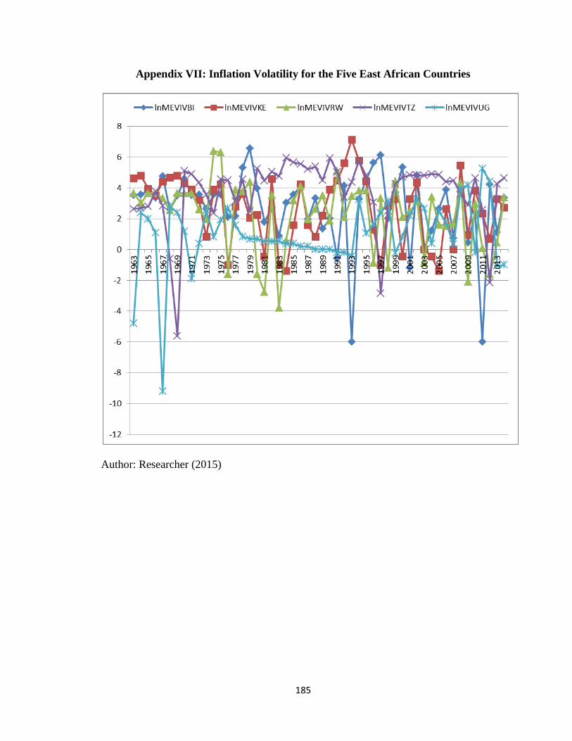
185

Appendix VII: Inflation Volatility for the Five East African Countries

Author: Researcher (2015)

186

Appendix VIII: Exchange Rate Volatility for the Five East African Countries

Author: Researcher (2015)