WP/08/6

Financial Instruments to Hedge Commodity Price Risk for Developing

Countries

Yinqiu Lu and Salih Neftci

© 2008 International Monetary Fund WP/08/6 IMF Working Paper

Monetary and Capital Markets Department

Financial Instruments to Hedge Commodity Price Risk for Developing Countries

Prepared by Yinqiu Lu and Salih Neftci1

Authorized for distribution by Udaibir S. Das

January 2008

Abstract

This Working Paper should not be reported as representing the views of the IMF. The views expressed in this Working Paper are those of the author(s) and do not necessarily represent those of the IMF or IMF policy. Working Papers describe research in progress by the author(s) and are published to elicit comments and to further debate.

Many developing economies are heavily exposed to commodity markets, leaving them vulnerable to the vagaries of international commodity prices. This paper examines the use of commodity options—including plain vanilla, risk reversal, and barrier options—to hedge such risk. It then proposes the use of a new structured product—a sovereign Eurobond with an embedded option on a specific commodity price. By extracting commodity price risk out of the bond, such an instrument insulates the bond default risk from commodity price movements, allowing it to be marketed at a lower credit spread. The product is also designed to help developing countries establish a credit derivatives market, which would in turn enhance the marketability and liquidity of sovereign bonds.

JEL Classification Numbers: G10, G13, G15 Keywords: Developing economies, commodity risk, options, debt instrument, credit default

swaps. Authors’ E-Mail Addresses: ylu@imf.org; sneftci@gc.cuny.edu

1 Professor Salih Neftci is at the City University of New York. We thank Eduardo Borensztein, Jorge Chan-Lau, Stijn Claessens, Udaibir S. Das, Randall Dodd, Dhaneshwar Ghura, Francois Haas, Joannes Mongardini, Andre Santos, and Amadou Sy for their comments and suggestions. All errors and omissions remain our sole responsibility.

2

Contents Page

I. Introduction ............................................................................................................................3

II. Smooth fluctuations in Commodity Revenue Collections—Option Transactions................4 A. Plain Vanilla Options ................................................................................................5 B. Risk Reversals ...........................................................................................................7 C. Barrier Option Structures ..........................................................................................9

III. Smooth Borrowing Cost—A Structured Product ..............................................................11 A. The Instrument ........................................................................................................12 B. Intermediary ............................................................................................................13 C. Pricing .....................................................................................................................14

IV. Conclusions........................................................................................................................18

References................................................................................................................................19 Tables 1. Prices of ATM Options..........................................................................................................7 2. Prices of 20 Percent OTM Options........................................................................................7 3. Prices of the Up-and-Out Put Options: H=120......................................................................9 4. A-Priori Parameters .............................................................................................................16 Figures 1. A Put Option Structure...........................................................................................................6 2. A Zero Premium Risk Reversal Structure .............................................................................8 3. A Knock-out Option ............................................................................................................10 4. The Structure of the New Instrument...................................................................................13 5 The Involvement of Investment Bank as an Intermediary....................................................14 6. Option Premium: 5.0−=ρ ..................................................................................................17 7. Option Premium: H = 70 .....................................................................................................17

8. Option Premium: 2.0=Xσ .................................................................................................18

3

I. INTRODUCTION

Developing countries produce and export a large amount of raw material commodities, such as crude oil (Venezuela, Nigeria, and the Republic of Congo), copper (Chile and Zambia) and agricultural commodities, such as tobacco (Malawi) and cocoa (São Tomé and Principe). In particular, some developing countries’ exports are highly concentrated in one or two leading commodities (Cashin, Liang, and McDermott 1999). This heavy reliance on commodities exposes these economies to price volatility in a form of terms of trade shocks, raising two related concerns. The first one is the large fluctuations in revenue collections, and the other is that it complicates public debt management. Either concern, if realized, will have an adverse impact on the economy (Becker, etc., 2007). The first concern is obvious. Price volatility is likely to affect the fiscal balances of economies whose revenues rely heavily on commodity-related taxes, royalties, and dividend income (in heavily state-owned commodity sectors). When commodity prices drop, revenue will fall, forcing countries to cut spending or incur debt. By contrast, a rise in commodity prices may create a revenue windfall, raising questions about an economy’s absorptive capacity and ways to spend the excess revenue. Some countries (Chile and Russia, etc.) have establishes a resource fund to save commodity-related revenue when prices are high and to draw money for budget support when prices are low. Resource funds tend to minimize budget disturbances resulted from price volatility and are a useful way to save resources for future generations, especially if the resources are nonrenewable. For an overview of nonrenewable resource funds and a review of their shortcomings, see Davis, Ossowski, Daniel, and Barnett (2001). Fasano (2000) summarizes six economies’ experience with resource funds and examines their contributions to public financial management. The second concern arises because governments cannot accurately predict future revenues and financing needs; therefore, they face difficulty in projecting external borrowing need. In the worst-case scenario, countries dependent of commodity revenues may not be able to make debt payments2 or may have to pay high interest rates for new external debt when price shocks cause fiscal balances to deteriorate, the exact time that they need resources for financing. Some debt instruments could address this concern by linking debt payment to commodity prices or the GDP growth rate–commodity-linked or GDP-linked bonds.3 Coupons and 2 It is noted that default is an option that a country may resort to under certain conditions. In this paper, we assume that costs of default are too huge for the country to cash the option of default.

3 For descriptions about commodity-liked bonds, see O’Hara (1984), Atta-Mensah (2004), and Privolos and Duncan (1991). For description and benefits of GDP-linked bonds, see Borensztein and Mauro (2004).

4

principal payment of commodity-linked bonds are linked to a stated amount of a reference commodity. Because the volume is fixed, a country’s debt payment is positively related to its export commodity prices; as a result, its debt burden declines following the plunge of commodity prices. However, the pools of investors willing to have exposure to commodity risks are smaller than those invest in traditional bonds. The GDP-linked debt instrument allows countries to adjust debt payment to their growth rates. If a drop in commodity prices causes growth to slow, countries can pay less. In this paper, as regards the first concern: large fluctuations in revenue collections, it explores three types of option transactions that can be used to smooth revenues.4 The first hedging measure we consider is very straightforward but costly—using plain vanilla put or call options on the relevant commodities. The second is to buy structured option products, which lower the high cost of plain vanilla options by selling other options simultaneously. We use risk reversal as an example. Such structures are cost-effective but may introduce other risks. The third approach is to use barrier options to manage commodity price risk. Then, to smooth the volatility of borrowing cost, the second concern, we introduce a new structured product—a sovereign Eurobond with embedded option on commodity prices. This product is constructed in a way that keeps adverse price movements from affecting the country’s ability to get external funds. Therefore, by enabling the country to smooth debt cost and maintain its cash flow at a reasonable cost, it is ready to finance a deficit. Moreover, the embedded option uses credit derivatives as the underlying instruments,5 of which market development may help create some liquidity conducive for sovereign bond market development.6

II. SMOOTH FLUCTUATIONS IN COMMODITY REVENUE COLLECTIONS—OPTION TRANSACTIONS

Commodity derivatives are widely regarded as a way to hedge commodity price volatility. Firms can take a position on commodity derivates to protect against an undesirable outcome. Stulz (2002) shows that derivatives are also widely used by companies for risk management. Suppose an airline company wants to hedge against the rising cost of jet fuel, it could lock in an agreed price with fuel suppliers for its purchase price through derivatives.

4 There are equal reasons to hedging imports as they are disruptive too.

5 According to British Bankers’ Association estimates, starting from 2005, the notional global amount of credit derivatives has been larger than the global amount of debt outstanding.

6 For example, Kazakhstan has a CDS market even though it does not have outstanding sovereign bonds.

5

Countries could also use derivatives to smooth commodity-related revenues. Daniel (2001) explains why hedging in oil price risk markets could be a solution to transfer the oil price risk from oil producing countries to others that are better to bear it. Some countries have used commodity derivatives to smooth future revenues. As documented by Larson, Varangis, and Yabuki (1998), many developing countries have begun using commodity derivatives markets to hedge commodity price risks. For example, Chile’s state-owned company, Codelco (the world’s largest copper producer), is already active in copper risk management. Moreover, cotton futures and options could serve as a risk management instrument for Africa’s cotton-producing countries (Satyanarayan, Thigpen, and Varangis 1993). Claessens and Duncan (1984) draws many case studies to demonstrate that developing countries can benefit significantly from using financial instruments to manage their risk. Moreover, commodity import countries could also use derivatives to smooth their expenditure on commodities. Nevertheless, three factors inhibit the wider use of commodity derivatives by countries. The first factor is that the markets for commodity options are rather limited in size and depth, and are therefore unlikely to be able to accommodate the needs of all the commodity-exporting countries. The second factor is the political constraints; the political costs of hedging may outweigh the benefits. As pointed by Daniel (2001), in the case of a fall in the commodity price, any gains from derivatives transactions may be seen as speculative returns. In the case of price rising, any hedging instrument may result in foregoing higher revenues. The last factor is the cost considerations. The purchase of futures requires the deposit of margins and the purchase of options requires a premium payment. This section first presents the use of plain vanilla options to hedge commodity risk and points out that the high cost could inhibit their usages. This is followed by two additional approaches that could reduce the cost of hedging significantly.

A. Plain Vanilla Options

In vanilla options, a put option provides insurance against drops in commodity prices, while a call option insures against unfavorable price hikes. Hedging can be achieved by choosing a proper strike price, K, and adjusting its level and at the same time as the cost of this insurance. Table 1 lists the prices of at-the-money (ATM) options7 on some selected commodities. The volatilities given in table 1 were from the Bloomberg for the month of November 2006. The risk-free interest rate r was 5.2 percent. In addition, we assume that the convenience yield8 is 7 These are options with strike price equaling the spot price.

8 The convenience yield is an imputed yield on the underlying instrument because warehousing commodities is apparently a convenient facility for the commodity user.

6

the same as the storage cost per unit. Here, numbers under “strike” mean percentage of the underlying price.9 The option prices, which can be interpreted as the percentage of the underlying nominal amount, are derived using the Black-Scholes formula (Black and Scholes, 1973), given by:

TddT

TrKXd

dNXdNKep

T

TrT

σσ

σ−=

++=

−−−= −

12

2

1

12

,)2/()/ln(

)()(

0

0

Where p is the price of the put option at 0T , and N(x) is the cumulative probability distribution function for a standard normal distribution.

0TX is the spot price of underlying

instrument at 0T , σ is the volatility, and T is the maturity of the option.

Figure 1. A Put Option Structure

9 The underlying price is the futures price instead of spot price. Traders write options on futures because the commodity futures market is more liquid then the spot market.

KCopper price

Option payoff

Put premium

Put option value before expiration

Option payoff at expiration

K

K

Effective price

Copper price

7

Table 1. Prices of ATM Options

Commodity Strike Volatility Price of 1-year

maturity Price of 3-year

maturity Copper 100 38.2% 12.4 17.5

Oil 100 16.3% 4.1 4.8 Gold 100 21.1% 5.9 7.5

Figure 1 shows the payoff of a plain vanilla put option. By buying a put option, the country locks in a floor of price, K. As suggested by the prices in Table 1, ATM commodity put options are expensive. By contrast, options 20 percent out-of-the-money (OTM) are less expensive than ATM commodity put options (Table 2).10 According to Tables 1 and 2, buying a three-year, 20 percent out-of-the-money option for insuring an underlying portfolio of US$500 million will cost about US$11 million for gold, close to US$5 million for oil, and US$47 million for copper. Though half those connected to ATM options, the costs are still high. If a country’s copper sector contributes 50 percent of GDP, and the country uses OTM options to hedge all of its gold output, an OTM hedging strategy would cost the country 5 percent of GDP, a burdensome amount for any developing economy. As a result, the government may be quite reluctant to hedge the commodity price risk. If the price movements turn out to be favorable, the cost and losses involved in options could exert great political pressure on the government. Daniel (2001) elaborates on the political pressure faced by the Ecuadorian authorities in early 1993 stemming from losses connected to the option and swap deals conducted by the central bank and the monetary board.

Table 2. Prices of 20 Percent OTM Options

Commodity Strike Volatility Price of 1-year maturity

Price of 3-year maturity

Copper 80 38.2% 4.6 9.4 Oil 80 16.3% 0.3 1.0

Gold 80 21.1% 0.8 2.3

B. Risk Reversals

A traditional way to cut option costs is to sell other options, so that the earnings from the short position will lower the insurance cost of the long option position. Risk reversal (RR) is one example of a zero-cost structure. As an example, we consider one country whose economy is heavily dependent on copper. Given that a plunge in world copper prices would

10 A 20 percent out-of-the-money put will start providing insurance after the commodity prices fall more than 20 percent.

8

severely affect the country’s fiscal balance and current account, the country enters into option transactions to hedge the copper price risk. Let the current copper price index be 100, and the country decides to buy a long-dated 20 percent OTM put with strike 80 on copper for US$500 million. The cost of such a three-year option position would be US$47 million. To cut those costs, the government could sell an OTM call with a strike price of 120. The sale of the 20 percent out-of-the-money call will raise US$47 million if we ignore the volatility smile,11 yielding a net portfolio cost of zero. The structure is called a zero premium collar (Figure 2). In this case, the country is fully hedged for any price below 120.

Figure 2. A Zero Premium Risk Reversal Structure

11 Volatility smile refers to a pattern in which an ATM option tends to have lower implied volatility than OTM or ITM options.

Kc=120

Kp=80

Copper price

Option Payoff

Vanilla call

Vanilla put

Put premium

Call premium

Risk of unlimited losses

Effective price

Kp=80 Kc=120

Kp=80

Copper price

Kc=120

9

However, this structure carries some risk given that the effective price is capped at 120. Therefore, if copper prices climb steeply to more than 120, the instrument will begin to lose money, though the jump in copper prices would boost country’s revenues, enabling it to finance the call-option position. However, the risk of losing millions of dollars on hedging instruments during a favorable move in copper prices is likely to be both politically and financially unacceptable.

C. Barrier Option Structures

By introducing various barriers in plain vanilla contracts, creating instruments known as barrier options, we can fix the drawbacks of risk reversal approaches discussed above. We consider the following alternative to replace a risk reversal: the country chooses to buy a put option with a strike pK and a knock-out barrier H ( )

0HXK Tp << as shown in Figure 3).

This option is an up-and-out put, which gets knocked out or ceases to exist if the underlying asset price tX exceeds H during the life of the contract. Except for the knock-out property, the option is the same as a plain vanilla put option. Figure 3 shows the price of the up-and-out put together with a plain vanilla option. As HX t → , the up-and-out put price falls to zero. At time 0T , the cost of this barrier option falls below that of the plain vanilla option. The difference (Hull, 2002) is

.)]/(ln[

,2/

),()/()()/(difference

0

000

2

2

2

222

TT

KXHyr

TyNXHKeyNXHX

T

TrT

TT

λσσσ

σλ

σλλ

+=+

=

+−+−−= −−

Table 3 shows the price of the up-and-out put with H = 120. As the Table 3 shows, the prices are lower than those for plain vanilla put options.

Table 3. Prices of the Up-and-Out Put Options: H=120

Commodity Strike Volatility Price of 1-year maturity

Price of 3-year maturity

Copper 80 38.2% 3.8 5.5 Oil 80 16.3% 0.3 0.9

Gold 80 21.1% 0.8 2.0 An up-and-out put option is similar to a dynamically managed risk reversal. The country could enter a risk reversal by buying a plain vanilla pK - put and selling a plain vanilla cK -

call with the property that if tX reaches H; the two options will have the same value. Hence, if tX hits H, the country could sell the put and close the call position. In other words, at t the country could liquidate the portfolio at zero cost. The loss from the dynamically managed risk reversal is zero when tX exceeds H. This replication of risk reversal is exactly an

10

up-and-out put option. In the worst case, the country will bear some liquidation losses (gap risk), though such risk would be minimal. Hence, knock-out or knock-in features make options affordable and eliminate the drawbacks of risk reversals, albeit at a higher cost. Public entities in developing economies could therefore use such instruments to hedge commodity risk, without the political backlash of risk reversals.

Figure 3. A Knock-out Option

There are several other types of standard barrier options. A knock-in option comes into existence if a barrier is hit, and then the option becomes a plain vanilla one. Also the imbedded barrier positions may be different, and the barrier may be in the OTM region. Such options normally have benign hedge ratios and Greeks.12 But the barrier may also be in the 12 Greeks is a term that summarizes the sensitivity of the option price with respect to changes in various parameters and variables. The smoother Greeks are, the easier it is to hedge the option.

Knock-out put

H

Kc

Kp

Copper price

Option payoff

Vanilla call

Vanilla put

Put premium

Call premium

Kp

Kp H

Copper price

H

Effective price

11

in-the-money (ITM) region. For example, a reverse knock-out option gets knocked out when it is in the money. The sensitivities of such options are discontinuous, which may lead to hedging difficulties. Up-and-out call options, in which the barrier H is greater than the strike K, are also difficult to hedge. This type of product combines a discontinuous pay-off at the barrier with a positive or negative gamma,13 depending on the current spot and time to maturity. Barrier options can take various forms. For example, up-and-out and down-and-out barriers can be combined into one product, known as the double-no-touch knock-out, an option that expires if price touches any of the barriers. In partial barrier and forward-starting barrier options, barriers exist for only a portion of the option’s life. The main advantage of such products is that they lower hedging costs. The barrier options described above can also be combined to produce more complex products, such a multi-underlying barrier options or amortizing barrier options. Multi-underlying barrier options may be “in” or “out,” conditional on more than one underlying price. Such structures are especially useful for developing economies that are heavily dependent on two commodities. The amortizing barrier option may be useful to countries with exposure to sustained movements in commodity prices, as it is designed to earn or lose a fraction of its value, proportional to the time the underlying price is above the barrier. We can further modify barrier options by adding more complicated barriers. In a resettable barrier, for example, once one barrier is touched, another already known barrier gets activated. Such instruments give developing economies greater flexibility in hedging commodity risk.

III. SMOOTH BORROWING COST—A STRUCTURED PRODUCT

As regards a country highly dependent on commodity exports, its cost of external borrowing, especially credit spread, and commodity prices have relatively high correlation. When commodity prices are increasing, the improvement in sovereign balance sheet resulted from budget surplus and reserve accumulation could reduce the default risk, and therefore credit spread and borrowing cost, vise versa. If commodity prices can be de-linked from the credit spread of a country’s Eurobond, the default probability embedded in the Eurobond will not be affected by the commodity price movements. As a result, the country could tap into the international market at a reasonable cost even when the commodity price moves adversely, the time when financing is needed.

13 Gamma is the second derivative of the option price formula with respect to the underlying risk. It represents the curvature of the option. Delta is the first derivative of the option price with respect to the underlying risk.

12

One natural approach is to attach a commodity derivatives contact in the Eurobond. An easy way is to attach a plain vanilla put option so that when the commodity price decreases, bondholders mark to the market loss from the bond owing to increasing credit spread could be compensated by the gain from the option. However, the fact that the country is the underwriter of the option introduces counterparty risk for the investors, and therefore reduces the attractiveness of the instrument. The other way is for the bond investors to receive a commodity price linked option on a CDS, written on the sovereign issuer. This is supposed to protect bondholders against a default of the issuer without them paying for the CDS. As an exchange, bondholders would accept a lower credit spread. The country has to pay an upfront option premium to an intermediary. This structure could prevent the commodity price volatility from influencing the Eurobond’s credit spread, and smooth the country’s external borrowing cost. An additional advantage is that it would help market-making for credit instruments on developing countries. This section will discuss this instrument, the intermediary, and pricing issues.

A. The Instrument

The basic components of this instrument include (1) a standard Eurobond; (2) a digital option on commodity prices; and (3) a credit default swap (CDS). To extract some of the commodity price risk, we embed an option in a standard Eurobond. Current time is 0T , the option expires at 1T , and the bond has maturity of 2T . First, we assume that the bond with maturity 2T contains a European knock-in put option, in which the barrier gets activated once commodity prices reach the barrier. In particular, we assume that if the commodity price, tX , falls below a predetermined barrier level, H, anytime during ],[ 10 TTt ∈ , the bondholder will receive a digital put option14 with strike K (H <K). We then introduce a second component: at

1T , if the digital is in-the-money, KX T <1

, the bondholder has the right to receive a CDS

with a strike price of 0TS , while the market price of this CDS has reached

1TS . If 1TS is higher

than0TS , which is likely because the lower commodity price will have an adverse impact on

the economy, the bondholder, at 2T , has a positive payoff of 1TS -

0TS multiplying by the notional amount. The structure is shown in Figure 4. The price movements following line b and c knock in the digital, but only that movement following line b ends up ITM and receives a CDS with the premium

0TS .

14 A digital put option is an option in which the payoff is fixed after the price of the underlying instrument moves below the strike price.

13

This instrument has several characteristics. First, an option to hedge the commodity price decrease is needed only if (1) the commodity price falls sharply— HX t < , and (2) if this price drop is persistent—

1TX is still below K at 1T . Mild fluctuations and temporary drops in commodity prices may not divert the economy from its own implied path. Thus, a knock-in feature is added to increase the option’s relevance and also lower its price. Second, the option is digital, and the payoff is a CDS, features that protect the bondholders against a potential default if the commodity price decrease is sharp and permanent. In fact, the whole structure can be regarded as a knock-in CDS, where the knock-in feature is linked to a commodity price. Therefore, the commodity risk in the bond is stripped out from the bond price by introducing a CDS, making the bond bear lower default risk.

Figure 4. The Structure of the New Instrument

Third, the introduction of CDS may have long-term benefits. To the best of our knowledge, CDS markets operating in developing economies are not very liquid. No matter how illiquid or “artificial” at the outset, a CDS market could lead to a genuine market of sovereign Eurobonds. Nevertheless, the introduction of CDS in hedging instruments for developing economies also adds some pricing difficulties, because in most developing economies market data, such as a CDS spread term structure, do not exist.

B. Intermediary

As the sovereign issuer is not in a position to buy or sell the CDS to investors, some large investment bank with high credit rating can act as an intermediary (Figure 5). At 0T , a developing economy issues option-embedded bonds to investors. The investment bank promise to sell CDS at

0TS , specified at the inception of the bonds, to bondholders if the

St

b

c

a

T0 T1 Time

Price

H

K

ST1 ST0

Payoff from CDS at T2

14

embedded option turns out to be in the money at 1T . In other words, the bondholders have secured the default protection from a credible counterparty at a low and fixed price. Nevertheless, the investment bank has to buy CDS at

1TS from a CDS market maker. Their

expected loss should be compensated by a payment from the developing economy at time 0T . In an arbitrage-free environment, this payment to the investment bank should be equal to the price of the option embedded in the bond.

Figure 5. The Involvement of Investment Bank as an Intermediary

C. Pricing

To calculate the price that the developing economy has to pay to the investment bank, we need to calculate the price of the embedded option in the bond. Given the lack of data on developing economies’ CDS premium, the data required to price the option must be decided a priori. To simplify the pricing process, we assume that the bond matures after 02 TT − years and that the options expires after 01 TT − years. Therefore, if the option is in the money at 1T , the investment bank has to deliver CDS at 1T , and the first and only payment occurs at 2T . We set 12 TT − as one year, and the CDS contract here is assumed to be one year forward CDS.15 Figure 4 shows the expected value of the payoff. The payoff at 0T is given by

}]0),[({),( ],[,,20 10101 TTuKXHXTT TuISSMaxTTBNPayoff ∈≤≤×−××=

15 See Hull and White (2003) for the pricing for forward CDS.

Sell CDS priced as ST1 at T1 Make payment at T0

Sell bonds at T0

A developing economy

Investment

bank CDS seller

Bondholders

Sell CDS priced as ST0 at T1

15

Where N is the notional amount, ),( 20 TTB is the discount factor, ],[,, 101 TTuKXHX TuI ∈≤≤ is an

indicator function (1 when commodity price hits H during ],[ 10 TT and is below K at 1T ). The option is a path-dependent option, which means that the knowledge of final spot values are not sufficient to determine the payoff. Monte Carlo simulation is the natural way to price the option. Before conducting the simulation, we must choose (1) the CDS premium at 0T ; (2) the dynamic path for CDS premium; (3) the commodity prices at 0T ; (4) the dynamic path for commodity prices; and (5) and the correlation between commodity prices and CDS premiums. We assume that the dynamic paths for both the commodity price and the CDS premium follow mean-reverting lognormal processes, a method that give us two advantages. First, the simulated prices are always positive in a lognormal process. Second, traders naturally think volatilities arising from a lognormal distribution model rather than from a normal distribution model. Here we use the pre-determined values for all parameters being considered. To show the impact of the parameters on the final payoff, we derive prices using different parameter values. Owing to the developing economy’s high dependence on commodity prices, we impose a significant correlation between the two processes. Specifically, the dynamic processes for commodity price and CDS premium are

.

,)]ln([)ln(

,)]ln([)ln(

00

00

dtdWdW

SSdWdtSaSd

XXdWdtXaXd

sX

TTSStSSt

TTXXtXXt

ρ

σθ

σθ

=

=+−=

=+−=

By Ito’s lemma, we obtain

.

,)]ln(2

[

,)]ln(2

[

00

00

2

2

dtdWdW

SSdWSdtSaSdS

XXdWXdtXaXdX

sX

TTStStSS

Stt

TTXtXtXX

Xtt

ρ

σσθ

σσθ

=

=+−+=

=+−+=

ρ is negative because the adverse movement of commodity prices may mean higher default probability, which must be compensated by a higher CDS premium. The simulations show the effects of Xσ , H, and ρ on the option premium. We assume that the option has a notional amount of US$1 and that the values for the other parameters are the values in Table 4.

16

Table 4. A-Priori Parameters

Parameters Values

02 TT − 5

01 TT − 4

0TX 100

Xθ 1

Xa 0.2

Xσ 0.1—0.3

H 60—80 K 90

0TS 10%

Sθ -0.5

Sa 0.2

Sσ 0.2

ρ -0.1—(-0.9)

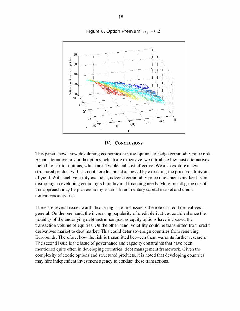
Figure 6 shows how the option premium varies with Xσ and H when ρ is held constant at the specified level. For the same H, the price of the option premium increases as Xσ moves up, because as volatility increases, X is more likely to drop to H, and the bondholder will receive a digital option. For a fixed Xσ , the option premium increases as H increases, because the higher the barrier (the closer to the spot price) goes, the more likely it is that the bondholder will receive the digital option. Figure 7 plots the option premium against Xσ and ρ for a given H. As before, the relationship with Xσ is positive. With respect to ρ , Figure 7 shows that the higher the negative correlation goes, the higher is the option premium. In other words, a higher absolute value of ρ means that a decline in commodity prices has a larger impact on credit spread, holding all other variables constant, and therefore a higher CDS premium. Figure 8 illustrates the effect on the option premium of varying H and ρ for a given value of Xσ . As before, the price relationships with H and ρ are positive.

17

Figure 6. Option Premium: 5.0−=ρ

Figure 7. Option Premium: 70=H

18

Figure 8. Option Premium: 2.0=Xσ

IV. CONCLUSIONS

This paper shows how developing economies can use options to hedge commodity price risk. As an alternative to vanilla options, which are expensive, we introduce low-cost alternatives, including barrier options, which are flexible and cost-effective. We also explore a new structured product with a smooth credit spread achieved by extracting the price volatility out of yield. With such volatility excluded, adverse commodity price movements are kept from disrupting a developing economy’s liquidity and financing needs. More broadly, the use of this approach may help an economy establish rudimentary capital market and credit derivatives activities. There are several issues worth discussing. The first issue is the role of credit derivatives in general. On the one hand, the increasing popularity of credit derivatives could enhance the liquidity of the underlying debt instrument just as equity options have increased the transaction volume of equities. On the other hand, volatility could be transmitted from credit derivatives market to debt market. This could deter sovereign countries from renewing Eurobonds. Therefore, how the risk is transmitted between them warrants further research. The second issue is the issue of governance and capacity constraints that have been mentioned quite often in developing countries’ debt management framework. Given the complexity of exotic options and structured products, it is noted that developing countries may hire independent investment agency to conduct these transactions.

19

REFERENCES Atta-Mensah, Joseph, 2004, “Commodity-linked Bonds: a Potential Means for Less-

Developed Countries to Raise Foreign Capital,” Working Paper 2004–20 (Ottawa: Bank of Canada).

Becker, Törbjörn I., Olivier Jeanne, Paolo Mauro, Jonathan David Ostry, and Romain

Ranciere, 2007, “Country Insurance: The Role of Domestic Policies,” IMF Occasional Paper 254 (Washington: International Monetary Fund).

Black, Fischer, and Myron Scholes, 1973, “The Pricing of Options and Corporate

Liabilities,” Journal of Political Economy, Vol. 81, pp. 637–59. Borensztein, Eduardo, and Paolo Mauro, 2004, “The Case for GDP-indexed Bonds,”

Economic Policy 19 (38), pp. 165–216. Cashin, Paul, Hong Liang, and C. John McDermott, 1999, “How Persistent Are Shocks to

World Commodity Prices?” IMF Working Paper 99/80 (Washington: International Monetary Fund).

Claessens, Stijn, and Ronald C. Duncan, 1994, Managing Commodity Price Risk in

Developing Countries, the Johns Hopkins University Press. Daniel, James A., 2001, “Hedging Government Oil Price Risk,” IMF Working Paper 01/185

(Washington: International Monetary Fund). Davis, Jeffrey, Rolando Ossowski, James Daniel, and Steven Barnett, 2001, “Stabilization

and Savings Funds fro Nonrenewable Resources,” IMF Occasional Paper 205 (Washington: International Monetary Fund).

Fasano, Ugo, 2000, “Review of the Experience with Oil Stabilization and Savings Funds in

Selected Countries,” IMF Working Paper 00/112 (Washington: International Monetary Fund).

Hull, John, 2002, Options, Futures, and Other Derivatives, 5th Edition (Upper Saddle River:

Prentice Hall). _____, and Alan White, 2003, “The Valuation of Credit Default Swap Options,” Journal of

Derivatives, Vol. 10, pp 40–50.

20

Larson, Donald F., Panos Varangis, and Nanae Yabuki, 1998, “Commodity Risk Management and Development,” Policy Research Working Paper WPS 1963 (Washington: World Bank).

O’Hara, Maureen, 1984, “Commodity Bonds and Consumption Risks,” Journal of Finance,

Vol. 39, pp. 193–206. Priovolos, Theophilos, and Ronald C. Duncan, 1991, Commodity Risk Management and

Finance, (Washington: World Bank). Stulz, René, 2002, Risk Management and Derivatives, South-Western College Publishing. Satyanarayan, Sudhakar, Elton Thigpen, and Panos Varangis, 1993, “Hedging Cotton Price

Risk in Francophone African Countries,” Policy Research Working Paper WPS 1233 (Washington: World Bank).