
Financial Health Economics - University of...
49
http://www.econometricsociety.org/ Econometrica, Vol. 84, No. 1 (January, 2016), 195–242 FINANCIAL HEALTH ECONOMICS RALPH S. J. KOIJEN London Business School, London, NW1 4SA, U.K. TOMAS J. PHILIPSON Irving B. Harris Graduate School of Public Policy, University of Chicago, Chicago, IL 60637, U.S.A. HARALD UHLIG University of Chicago, Chicago, IL 60637, U.S.A. The copyright to this Article is held by the Econometric Society. It may be downloaded, printed and reproduced only for educational or research purposes, including use in course packs. No downloading or copying may be done for any commercial purpose without the explicit permission of the Econometric Society. For such commercial purposes contact the Office of the Econometric Society (contact information may be found at the website http://www.econometricsociety.org or in the back cover of Econometrica). This statement must be included on all copies of this Article that are made available electronically or in any other format.
Transcript of Financial Health Economics - University of...

http://www.econometricsociety.org/
Econometrica, Vol. 84, No. 1 (January, 2016), 195–242
FINANCIAL HEALTH ECONOMICS
RALPH S. J. KOIJENLondon Business School, London, NW1 4SA, U.K.
TOMAS J. PHILIPSONIrving B. Harris Graduate School of Public Policy, University of Chicago,
Chicago, IL 60637, U.S.A.
HARALD UHLIGUniversity of Chicago, Chicago, IL 60637, U.S.A.
The copyright to this Article is held by the Econometric Society. It may be downloaded,printed and reproduced only for educational or research purposes, including use in coursepacks. No downloading or copying may be done for any commercial purpose without theexplicit permission of the Econometric Society. For such commercial purposes contactthe Office of the Econometric Society (contact information may be found at the websitehttp://www.econometricsociety.org or in the back cover of Econometrica). This statement mustbe included on all copies of this Article that are made available electronically or in any otherformat.

Econometrica, Vol. 84, No. 1 (January, 2016), 195–242
FINANCIAL HEALTH ECONOMICS
BY RALPH S. J. KOIJEN, TOMAS J. PHILIPSON, AND HARALD UHLIG1
We provide a theoretical and empirical analysis of the link between financial andreal health care markets. This link is important as financial returns drive investment inmedical research and development (R&D), which, in turn, affects real spending growth.We document a “medical innovation premium” of 4–6% annually for equity returns offirms in the health care sector. We interpret this premium as compensating investors forgovernment-induced profit risk, and we provide supportive evidence for this hypothesisthrough company filings and abnormal return patterns surrounding threats of govern-ment intervention. We quantify the implications of the premium for the growth in realhealth care spending by calibrating our model to match historical trends, predicting theshare of gross domestic product (GDP) devoted to health care to be 32% in the longrun. Policies that had removed government risk would have led to more than a doublingof medical R&D and would have increased the current share of health care spendingby more than 3% of GDP.
KEYWORDS: Medical innovation, healthcare spending, risk premia.
1. INTRODUCTION
IMPROVEMENTS IN HEALTH HAVE BEEN A MAJOR COMPONENT of the overallgain in economic welfare and the reduction in world inequality during the lastcentury (Murphy and Topel (2006) and Becker, Philipson, and Soares (2005)).Indeed, an emerging literature finds that the value of improved health is on parwith many other forms of economic growth during the last century, as repre-sented by material per capita income reflected in conventional gross domesticproduct (GDP) measurements. As such, the increase in the quantity and qual-ity of life might be the most economically valuable change of that century. Atthe same time, the current size of the health care sector, now close to a fifthof the U.S. economy, and its continued growth have given rise to concernedpublic debates.
Medical innovation and its demand are central to these improvements inhealth and the expansion of the health care sector. Through medical progress,including improvements in knowledge, procedures, drugs, biologics, devices,and the services associated with them, there is an increased ability to prevent
1We are grateful to the late Gary Becker, Amy Finkelstein, Francisco Gomes, John Heaton,Casey Mulligan, Jesse Shapiro, Amir Sufi, Stijn Van Nieuwerburgh, Pietro Veronesi, Rob Vishny,Moto Yogo, both the editor and three anonymous referees, and seminar participants at Stan-ford, “Hydra Conference” on Corsica (2012), Bonn University, Columbia University, HumboldtUniversity (Berlin), Federal Reserve Bank of Philadelphia, MIT, the Milken Institute, Universityof Chicago, Wharton, USC, Yale, TED-MED, and the American Enterprise Institute for usefuldiscussions and suggestions. Koijen acknowledges financial support from the European ResearchCouncil (Grant 338082). Philipson acknowledges financial support from the George J. StiglerCenter for the Study of the Economy and the State, University of Chicago. Uhlig acknowledgesfinancial support from the NSF (Grant SES-1227280) and INET (Grant INO1100049).
© 2016 The Econometric Society DOI: 10.3982/ECTA11182

196 R. S. J. KOIJEN, T. J. PHILIPSON, AND H. UHLIG
and treat old and new diseases. Many analysts emphasize that this surge inmedical innovation is key to understanding the rapid expansion of the healthcare sector (Newhouse (1992), Cutler (1995), and Fuchs (1996)).
Therefore, to understand the growth of this sector, and the medical researchand development (R&D) that induces it, it is important to understand the fi-nancial returns of those investing in medical innovation. This paper providesthe first quantitative analysis of real and financial health care markets by ex-amining the joint determination of the financial returns of firms that invest inmedical R&D and the resulting growth of the health care sector.
We first provide empirical evidence that the returns on firms engaged inmedical R&D are substantially higher, around 4–6% per annum, than thosepredicted by standard empirical asset pricing models, such as the capital assetpricing model (Sharpe (1964)) and the Fama and French (1992) model. Thislarge “medical innovation premium” suggests that investors in the health careindustry need to be compensated for nonstandard risks.
We provide a potential interpretation of the medical innovation premiumas resulting from government risk for which investors demand higher returnson health care firms beyond standard risk-adjusted returns. In particular, weconsider government-induced profit risk to be a plausible explanation for themedical innovation premium for three reasons. First, government greatly af-fects both the onset of profits through approval regulations and the variableprofits conditional on such approval though reimbursement policies. For exam-ple, demand subsidy programs such as Medicare and Medicaid currently makeup about half of medical spending in the United States and, thus, are clearlyan important component affecting the profits of innovators. Second, we seekan aggregate risk component to which the health sector is particularly exposed.Government-induced profit risk has that property. Third, we discuss that sev-eral other plausible risk factors, such as, for instance, longevity risk, often implya negative medical innovation premium in standard consumption-based assetpricing models, which is the opposite sign of the premium we document.
We provide supportive evidence for the hypothesis that government risk con-tributes to the medical innovation premium in three ways. First, we provide atext-based analysis of financial statements (10-K filings) that companies filewith the Securities and Exchange Commission (SEC). The 10-K filings con-tain a section that asks the company about the risk factors it faces. We showthat firms in the health care sector discuss government-related risk significantlymore frequently than firms in other sectors. Second, we find that investors ex-perience large negative returns when there are severe threats of governmentintervention.2 Third, examining the proposed Clinton health care reforms ofthe 1990s, we find that health care firms experienced abnormally low returns.Moreover, firms with more negative (abnormal) returns during this period,
2See also Ellison and Mullin (2001) and Golec, Hegde, and Vernon (2010), and the proposedClinton health care reform as a key example.

FINANCIAL HEALTH ECONOMICS 197
which are, therefore, firms that are more sensitive to government interven-tion risk, are generally more exposed to the health care factor that earns themedical innovation premium. This finding is consistent with our interpretationof the medical innovation premium as compensation for government-inducedprofit risk.
Our theoretical analysis then investigates the link between financial markets,the incentives for medical innovation it induces, and real health care marketsin terms of its growth resulting from this innovation. We analyze the quantita-tive growth of the health care sector when investors face government-inducedprofit risk. The model developed in this paper is a two-sector version of a rare-disaster model.3 The economy has a large sector outside of health care thatis free from disaster risk (in fact, for simplicity, free of any risk) and a smallerhealth-care sector that faces a nontrivial probability of disaster. That disaster isgovernment intervention that wipes out, or substantially reduces, shareholdervalue in the sector. This is a disaster from the perspective of the investors only,as opposed to society as a whole. With an artfully chosen stochastic discountfactor for the investors, the model delivers the observed medical innovationpremium. The medical innovation premium predicted by the model has twoparts: an actuarially fair disaster premium and the risk premium arising fromthe entrepreneurial consumption reduction in the wake of the disaster. We ar-gue that a standard capital asset pricing model (CAPM) regression or a Fama–French regression finds a substantial excess return (alpha) for the disaster-prone sector mainly because of the latter, that is, mainly because of the adversecorrelation with the stochastic discount factor.
We find that the estimated medical innovation premium has large effects onhealth care spending and medical R&D by calibrating our model to observedtime trends from 1960 to 2010. In particular, we find that the size of the healthcare sector would have increased by 3% of GDP if government interventionrisk had been removed and we show that the larger part of it is due to the en-trepreneurial risk premium as opposed to the actuarially fair disaster premium.Furthermore, our calibration implies that R&D would more than double inthe absence of the medical innovation premium, where once again the riskpremium explains the bulk of the difference. This reduction in medical R&Dinvestments in the presence of the medical innovation premium provides a po-tential explanation for the “missing R&D” implied by the analysis by Murphyand Topel (2006), which suggests that the enormous value of gains in healthjustify much larger investments in medical R&D than are actually observed.
By 2050, our model suggests that 27% of GDP is spent on health care, con-ditional on no government intervention. The long-run steady state share isslightly below 32% of GDP. The Congressional Business Office (CBO) projects
3The rare-disaster approach has been used in a number of recent papers to explain equitypremia; see, for instance, Barro and Ursua (2008), Barro and Jin (2011), or Gabaix (2012). Weapply this idea specifically to the health care sector.

198 R. S. J. KOIJEN, T. J. PHILIPSON, AND H. UHLIG
that total spending on health care would rise from 16% of GDP in 2007 to 37%in 2050 and 49% in 2082. Hence, our model produces estimates for the healthcare share that are somewhat lower than the CBO projections.
2. INSTITUTIONAL BACKGROUND
Technological change that raises health care spending mainly comes fromthree categories: medical devices, biologics, and drugs, and the services as-sociated with them. In the United States, the variable profits on these newtechnologies are determined both by private and public reimbursement poli-cies. According to the Centers for Medicare and Medicaid Services (CMS),in 2012 about 44% of U.S. spending was publicly financed, mainly throughthe Medicare and Medicaid programs. However, returns in other parts of theworld are more contingent on public reimbursement policies. For example, inEuropean countries, roughly 85% of health care is publicly financed (OECD,2013).
New health care products are often discovered by academic research; how-ever, the high cost of development of medical products relies on outside in-vestors, whose main focus is on (risk-adjusted) earnings. Hence, even thoughthe research (“R”) in medical R&D may not be motivated entirely by futurereturns, the development (“D”) certainly is. Indeed, drugs and biologics areamong the most R&D intensive industries in the United States.
To raise capital for the large development costs, manufacturers often usepublic capital markets. It is important to note that much of the productionof goods and services in health care are not financed through public equitymarkets. Providers of hospital services, making up about a 35% of health carespending, are about 70% not-for-profit and thus rely on debt or donationsinstead of public equity. Physician services, making up an additional 22% ofhealth care spending (CMS 2012), are often organized in small privately fi-nanced clinics. Given the lack of public equity financing in these major healthcare sectors, it is understandable that the for-profit firms engaged in medicalinnovation make up a large majority of the firms listed on public equity ex-changes.
Government policies in the United States disproportionally affect the re-turns on medical R&D investments as world sales for medical products arehighly concentrated in the United States. Egan and Philipson (2013) use datafrom the World Bank and the World Health Organization to estimate that U.S.health care spending was about 48% of world spending in 2012 even thoughU.S. GDP was only about 24% of world GDP in the same year. For biophar-maceutical spending, the U.S. share of world spending is lower at about 39%,as many emerging markets spend a larger share of their overall health care onbiopharmaceuticals. Given the larger markups on U.S. spending, a larger shareof profits than sales is generated in U.S. markets. Because of the concentrationof world profits in the United States, changes in reimbursement policies that

FINANCIAL HEALTH ECONOMICS 199
threaten U.S. markups are of primary importance to those investing in medicalR&D. This motivates our focus on the risk of U.S. government reimbursementpolicies on asset prices.
3. EMPIRICAL EVIDENCE: THE MEDICAL INNOVATION PREMIUM
3.1. Risk Premia in Health Care Markets
To estimate the medical innovation premium, we use data on industry re-turns, the Fama and French factors, and market capitalization from KennethFrench’s website. The first classification we use splits the universe of stocks intofive industries: consumer goods, manufacturing, technology, health care, and aresidual category “other.”
The health care industry includes medical equipment,4 pharmaceutical prod-ucts,5 and health services.6 We also study Kenneth French’s classification into48 industries, which splits the health care industry into the three aforemen-tioned categories. We follow the industry classification as on Kenneth French’swebsite for both the entire health care industry and for the three subindustries.
We first study the returns of firms in the health care industry. In computingthe returns to health care companies, we correct for standard risk factors toaccount for other sources of systematic risk outside of the model. Therefore,we are interested in the intercepts, or “alphas,” of the standard time-seriesregression
rt − rf t = α+β′Ft + εt�(1)
where Ft is a set of risk factors, rt is the equity return, and rf t the risk-free rate.We are interested in the returns of health care firms relative to firms that arenot in the health care industry. To compute the relative returns, we regress thereturns on a constant, the alpha, and a set of benchmark factors, Ft . The alphameasures the differential average return of health care firms that cannot beexplained by standard asset pricing models.
Asset pricing models are distinguished by the pricing factors Ft they accountfor. As a first model, we use the excess return on the Center for Researchin Security Prices (CRSP) value-weighted return index, which comprises allstocks traded at AMEX, NYSE, and Nasdaq. This is a common implementa-tion of the capital asset pricing model (CAPM); see Sharpe (1964). The sec-ond benchmark asset pricing model we consider is the three-factor Fama and
4The corresponding standard industrial criterion (SIC) codes are 3693: X-ray, electromedicalapp., 3840–3849: Surgery and medical instruments, 3850–3851: Ophthalmic goods.
5The corresponding SIC codes are 2830: Drugs, 2831: Biological products, 2833: Medicalchemicals, 2834: Pharmaceutical preparations, 2835: In vitro, in vivo diagnostics, and 2836: Bio-logical products, except diagnostics.
6The corresponding SIC codes are 8000–8099: Services—health.

200 R. S. J. KOIJEN, T. J. PHILIPSON, AND H. UHLIG
French (1992) model, which is labeled Fama–French. In addition to the marketfactor, this model also accounts for firm size and the value factor. Empirically,smaller firms and firms with high book-to-market ratios, that is, value firms,tend to have higher average returns that are not explained by differences inCAPM betas. These additional two factors account for these regularities inasset markets.7
We present our main results for annual returns, using the Fama and Frenchmodel, and for the sample from 1961 to 2012, which is the period for whichwe observe health care spending. As the risk-free rate, rf�t in equation (1), weuse the 1-month T-bill rate from Ibbotson and Associates, Inc., rolled over for12 months as constructed by Kenneth French and available from his website.As the return per industry, rt in equation (1), we use the value-weighted returnof all stocks in a given industry.
The results are reported in panel A of Table I. The first line corresponds tothe alpha and the second line reports the t-statistic using ordinary least squares(OLS) standard errors. We find that the health care industry earns an econom-ically and statistically significant alpha of 5.0% (with a t-statistic of 2.4) relativeto the Fama and French model.
We also report the alphas of the other industries and find that they do nothave large alphas relative to the standard models. We conclude that there is arisk premium for holding health care stocks that cannot be explained by stan-dard asset pricing factors.
If we remove health services and focus on medical R&D more specificallythrough equipment and pharmaceutical products, the alphas are even higher at6.4% and 5.4% per annum, respectively. This is because the alphas on medicalservices are close to 0, which lowers the overall alpha of the health care sector.8
Both alphas are statistically significant at conventional significance levels.Although both subsectors, that is, medical equipment and drugs, earn signif-
icant alphas, these alphas are not necessarily driven by exposures to the samerisk factor. To test this more directly, we augment the Fama and French modelwith the health care factor, which we define as the industry return on the entirehealth care sector in excess of the risk-free rate.
We report the alphas of the subsectors relative to the augmented Fama andFrench model in panel B of Table I. We find that the alphas are economicallyand statistically close to 0 once the health care factor is included in the model,
7There is a large literature that provides explanations for the size and value effects; see, forinstance, Berk, Green, and Naik (1999), Zhang (2005), Yogo (2006), Lettau and Wachter (2007),and Koijen, Lustig, and Van Nieuwerburgh (2012). In this paper, we are particularly interested inthe risk premium in the health care industry above and beyond the standard risk factors, and wedo not provide an explanation for the market, size, and value risk premia or exposures.
8The returns on services start only in the late sixties and we, therefore, exclude them from thetable. However, their returns are well explained by standard asset pricing models and the alphasare close to 0.

FIN
AN
CIA
LH
EA
LTH
EC
ON
OM
ICS
201
TABLE I
INDUSTRY ALPHASa
Consumer Goods Manufacturing HiTec Health Other Medical Equipment Drugs
Panel A: Industry alphas relative to the CAPM and the Fama and French modelCAPM 1�81 1�66 −0�83 3�31 0�22 3�71 3�70T -statistic 1�40 1�54 −0�54 1�61 0�17 1�40 1�78Fama and French −0�13 1�04 1�67 5�01 −2�66 6�44 5�37T -statistic −0�09 0�84 0�86 2�44 −2�75 2�05 2�63
No. of observations 52 52 52 52 52 52 52
Panel B: Industry alphas relative to models extended with the health care factorCAPM + HC factor 0�22 0�31T -statistic 0�14 0�71FF + HC factor 0�81 0�37T -statistic 0�47 0�70
No. of observations 52 52aThe table reports in panel A the alphas relative to the CAPM and the three-factor Fama and French model for different industries. The sample is from 1961–2012 and returns
are annual. The first five industries add up to the market. The last two columns report the alphas of two subsectors of the health care sector: medical equipment and drugs. Inpanel B, we add the health care sector to either the CAPM or the Fama and French model, and report the alphas of both subsectors of the health care sector.

202 R. S. J. KOIJEN, T. J. PHILIPSON, AND H. UHLIG
which is consistent with the interpretation that the same risk factor drives thealphas in both subsectors.
Our results are consistent with the findings in Fama and French (1997), whostudy the performance of the Fama and French (1992) model for a large crosssection of 48 industries. Their Appendix B shows that the model is rejectedin particular due to two industries: real estate and health care. Despite thegrowing literature on returns in real estate markets, little is known about healthcare markets in this context.
For robustness, we estimate the model also at a monthly frequency and fortwo additional sample periods for annual returns, namely from 1927 to 2012and from 1946 to 2012. The first sample period is the longest sample available.The second sample focuses on the post-war period. Furthermore, we computethe alphas not only relative to the Fama and French model, but also relativeto the CAPM. The results for monthly returns and other sample periods arereported in the Supplemental Material (Koijen, Philipson, and Uhlig (2016)),but the results are broadly consistent with the findings reported in Table I. Ifwe use monthly data or longer sample periods, the statistical significance of thealphas increases.
3.2. Government Risk and the Health Care Sector
In this section, we provide new evidence on the importance of governmentrisk for firms in the health care industry.
3.2.1. Risk Factors Identified From 10-K Filings
Our first piece of new evidence comes from a text-based analysis of 10-K re-ports that each firm files annually with the Securities and Exchange Committee(SEC).9 We use the 10-K filings for 2012. As a robustness check, we also usethe 10-K filings for 2006, which is before Obamacare was discussed and beforethe financial crisis to ensure that our results are not driven by the recent healthcare reforms or regulation that followed the financial crisis.
In each 10-K filing, there is a Section 1.A labeled “Risk Factors.” The guide-lines for this section are described in Regulation S-K, Item 503(c), requestingcompanies to list the “most significant factors” that affect the future profitabil-ity of the company.
To illustrate the data we use in this section, we include the “Risk Factors”section of the 10-K filings of Pfizer and Apple, which are among the largest
9The 10-K filings have been explored recently in the finance literature to define industries(Hoberg and Phillips (2011)), to measure competition (Feng Li and Minnis (2013)), to predictthe volatility of stock returns (Kogan, Levin, Routledge, Sagi, and Smith (2009)), and to predictfuture stock returns (Loughran and McDonald (2011)).

FINANCIAL HEALTH ECONOMICS 203
TABLE II
DICTIONARY FOR 10-K FILINGSa
Dictionary to Identify Government Risk
Congress Government regulation(s) Political risk(s)Congressional Government approval PoliticsDebt ceiling Government debt(s) Price constraint(s)Federal Government deficit(s) Price control(s)Federal funds Government intervention(s) Price restriction(s)Fiscal imbalance(s) Law(s) Regulation(s)Government(s) Legal RegulatoryGovernment-approved Legislation Regulatory complianceGovernment-sponsored Legislative Regulatory delay(s)Governmental Legislatory Reimbursement(s)Governmental program(s) Patent law(s) SubsidyGovernment program(s) Political SubsidiesGovernmental regulation(s) Political reform(s)
aThe table reports the dictionary that we use to identify how frequently firms highlight risk factors that are associ-ated with government risk.
health and non-health care firms by the end of our sample, in the SupplementalMaterial.
As is clear from the filings, various forms of government regulation are a ma-jor concern to Pfizer, while for Apple, traditional risk factors such as economicconditions and competition are more relevant. Consistent with our model,Pfizer also explicitly mentions price controls and government intervention asone of the key risk factors that may affect the firm’s operations.
Generalizing beyond the illustration of Apple and Pfizer, we hand-collectthe sections on risk factors for the largest 50 health care companies and thelargest 50 non-health care companies. For each firm, we count the number oftimes words related to the government or government risk appear in the filings.
The dictionary that we use is summarized in Table II. The dictionary at-tempts to capture the prevalence of government-related risks in the 10-K fil-ings. In the main dictionary, we avoid words that are government-related yetparticular to the health care sector such as for instance “FDA” (Food and DrugAdministratioin), as this would bias our risk measurement toward the healthcare sector.
The results are summarized in panel A of Table III. For firms in the healthcare sector, we find that words in this dictionary appear roughly twice as muchin 2012, on average 130 times, compared to, on average, 77 times for firmsoutside the health care sector.
However, the typical 10-K filing for health care firms is longer. As an alter-native measure, we can look at the average fraction of words that appear in ourdictionary. For firms within the health care sector, this fraction is 1.55%, whileit is only 1.24% for firms in the non-health care sector, implying that words

204 R. S. J. KOIJEN, T. J. PHILIPSON, AND H. UHLIG
TABLE III
AVERAGE WORD COUNT TO MEASURE GOVERNMENT RISK FROM 10-K FILINGSa
Average Word Count Average Fraction of Words
Panel A: Main dictionary without health care-specific terms2006
Health care sector 76�36 1�46%Non-health care sector 35�46 0�93%
2012Health care sector 130�06 1�55%Non-health care sector 77�12 1�24%
Panel B: Dictionary including health care-specific terms2006
Health care sector 100�08 1�92%Non-health care sector 36�18 0�94%
2012Health care sector 165�56 1�97%Non-health care sector 79�72 1�29%
aPanel A of the table reports the average number of words in a firm’s 10-K filing that appear in the dictionary inTable II. The average is taken across the 50 largest firms in the health care sector and the 50 largest firms in the non-health care sector. The first column reports the average word count, while the second column measures the averagefractions of words (that is, word count scaled by the length of the document). Panel B reports the results if we expandthe dictionary to include government-related words that are specific to the health care sector. We report the resultsfor 2006 and 2012.
from our dictionary appear 25% more frequently for firms in the health caresector.
One concern one may have is that the higher fraction of government-relatedwords in 2012 is driven by the discussions around Obamacare. We thereforerepeat the entire exercise, but now for 2006, thus before President Obama waselected. Figure 1 shows the fractions for health care and non-health care firmsin both periods. We find that the fractions in both cases increase followingthe financial crisis, as one may expect. However, the fraction for non-healthcare firms increases substantially more (from 0.93% to 1.24%) than for healthcare firms (from 1.46% to 1.55%). These results suggest that our findings arenot just driven by risks related to Obamacare or changes in regulation thatfollowed the financial crisis.
As discussed, we omit government-related words from our main dictionarythat are particular to the health care sector. We also explore how our resultsare affected if we include the health care-specific terms “medicare,” “medi-care reform,” “medicaid,” “medicaid reform,” “PPACA,” “CMS,” “healthcarereform,” “NHS,” and “FDA” in our dictionary. The results for this expandeddictionary are reported in panel B of Table III. The differences in the averageword count and the average fraction increase substantially, making the differ-ences economically and statistically more significant.

FINANCIAL HEALTH ECONOMICS 205
FIGURE 1.—Fraction of government-related words in 10-K filings in 2006 and 2012.
Taken together, the text-based analysis of 10-K filings suggests that govern-ment risk is a relatively more important concern for firms in the health caresector.
3.2.2. Drawdowns of the Health Care Sector
Second, we study when financial investments in health care sector experi-enced large negative returns as a way to identify the risks to which the sector isexposed. In Figure 2, we plot the drawdowns for the health care sector along-side the drawdowns of the aggregate stock market. Drawdowns are defined as
Dt =t∑
u=1
ru − maxs∈{1�����t}
s∑u=1
ru�(2)
where rt denotes the log return on either the aggregate stock market or thehealth care sector. Hence, drawdowns measure the cumulative downturn rel-ative to the highest level the indexed reached up to a certain point in time.Drawdowns are a common way to measure the risk of investment strategies(see, for instance, Grossman and Zhou (1993), Landoni and Sastry (2013), andKoijen, Moskowitz, Pedersen, and Vrugt (2013)).

206 R. S. J. KOIJEN, T. J. PHILIPSON, AND H. UHLIG
FIGURE 2.—Drawdown dynamics for the health care sector and the aggregate stock market.The figure reports the drawdown dynamics of the health care sector and the overall stock marketfrom 1990 until 2013. Drawdowns are defined in equation (2).
Figure 2 points to three large downturns for the health care sector during thelast two decades: in the early nineties, during the 2000–2002 technology crash,and during the 2007–2008 financial crisis. During the latter two periods, thedrawdowns of the market are somewhat larger than those of the health caresector.
The drawdown in 1992 and 1993 is of most interest to us; it coincides withthe discussions around Clinton’s health care reform. During this period, theaggregate stock market increased, while the health care sector shows a largedecline.
Interestingly, we do not find a similar drawdown during the recent Obamareforms as during the proposed Clinton reforms. Hult and Philipson (2012)provide an explanation for these two opposing effects. They stress that gov-ernment expansions often lower both demand prices (premiums or copays)to raise access, but at the same time lower supply prices (reimbursements)through increased government monopsony power.
At the one extreme, when the poorest people are being added, the quantityeffect will dominate the markup effect, as the poorest were outside the pro-
FINANCIAL HEALTH ECONOMICS 207
gram. For example, Medicaid expansions have this positive effect on earningsand innovation. At the other extreme, when very rich individuals are added,their utilization will not be affected much by the lower demand price in thepublic program, but their markup will be lowered if they are subsumed under agovernment buyer. For example, the single-payer European payment systemsmay lower profits in this manner.
The nonmonotonic impact of government expansions across the income dis-tribution implies that Clinton’s reforms may affect returns in opposing waysthan do Obama’s reforms as represented by the different drawdown patterns.In particular, for the Affordable Care Act (ACA) under Obama, the Medi-caid expansions and the means-tested subsidies for exchange covered insur-ance raise the demand of the poor beyond market levels. Indeed, the CBOestimates that the ACA raises quantity, with most recent estimates suggestingthat the act raised insurance coverage by over 4 percentage points.10
More importantly, many investor reports from the financial services sectorupgraded valuations of medical R&D firms, citing the increase in demand in-duced by ACA.11 This may be one explanation of why the pharmaceutical in-dustry spent an estimated $150 million in lobbying efforts in support of theACA.12
In contrast, the Clinton health care plan, known officially as the Health Se-curity Act, was a 1993 health care reform package that centered on regulationsto provide universal and more homogeneous health care for all Americans,and also had as a major component overall price controls.
The proposed Clinton reforms are, therefore, closer in spirit to our discussedoverall markup threats and may be interpreted as more universally affectingthe entire income distribution, not only the poor parts of the population asin the means-tested reforms of the ACA. The extreme version of Clinton re-forms would have been universal public coverage such as in many Europeancountries, which would lead to the negative earnings effect discussed above.
Investment reports expressed concern over the potential negative effects theClinton plan would have on health care stocks,13 and we document that healthcare stocks responded negatively to this potential threat of price controls onmedical R&D firms. As opposed to the industry support for the ACA, whenClinton came to office, the trade organization Biotechnology Industry Orga-
10CBO (2014), “Updated Estimates of the Effects of the Insurance Coverage Provisions of theAffordable Care Act.”
11See, for instance, J. P. Morgan, “Global Biotech Outlook,“ Jan 6, 2014, BlackRock, “BGFWorld Health Science Fund,” 2012-Q1 Commentary, BlackRock, “Equity Dividend Fund,” 2014-Q1 Commentary, BlackRock, “North American Income Trust PLC,” Half Year Financial report,April 30, 2014, and Morgan Stanley, “On the Markets,” October 2013.
12See, for instance, http://www.nationalcenter.org/PR-JohnsonandJohnson_042811.html.13Pink Sheet, “Third Quarter FDC Index Is Mixed for Drugs as Fears of Clinton Spark Septem-
ber Swoon,” October 5, 1992.

208 R. S. J. KOIJEN, T. J. PHILIPSON, AND H. UHLIG
nization (BIO) was created as a response and lobbied extensively against theClinton health care plan.14
3.2.3. The Cross Section of Health Care Betas and Event Returns AroundClinton’s Health Care Reforms
Ellison and Mullin (2001) and Golec, Hegde, and Vernon (2010) also showthat health care stocks declined around the proposed Clinton reform in theearly nineties. These events provide a direct test of our theory, as the key com-ponent of the reform was to impose price controls on new drugs. Our objec-tive in this section is to show that firms that have higher health care betas,measured over periods much longer than the Clinton reforms, also experiencemore negative returns during these events. This result is relevant, as differentexposures to the health care factor measure different exposures to the risk fac-tor that result in the medical innovation premium. As differences in exposuresto the health care factor relate to differences in abnormal returns coming fromthreats of government intervention, government risk may be a reasonable can-didate determinant of the medical innovation premium.15
In our model, the exposure to the health care factor, which generates themedical innovation premium, and the exposure to government interventionrisk are one-for-one related, as government intervention risk is the only sourceof the risk premium. In reality, firms differ in their exposure to the health carefactor and in their exposure to government intervention risk. We abstract fromthis heterogeneity for simplicity and tractability in the model, but the hetero-geneity in the data allows us to test the link between the exposure to the healthcare factor and the exposure to government intervention risk.
Ellison and Mullin (2001) and Golec, Hegde, and Vernon (2010) identifythe key event dates during the Clinton reform proposals, which we reproducein Table IV. We first compute the health care beta, βHC
i , by regressing monthlyexcess returns of a given firm i on the market return and the health care factor,
rit − rf t = αi +βMi rMKT�et +βHC
i rHC�et + εit�(3)
where rMKT�et denotes the excess return on the aggregate stock market and rHC�e
t
denotes the excess return on the health care factor. We require firms to haveno missing monthly returns in 1991, 1992, or 1993, which is the period we usefor the event study. Also, consistent with the empirical asset pricing literature,we remove stocks with prices below $5 and above $1,000.
The regression in (3) provides us the exposure to the health care factor foreach firm, βHC
i . The typical sample to estimate the beta is much longer than
14BIO, “Milestones 2003: A History of BIO,” http://www3.bio.org/speeches/pubs/milestone03/.15Ideally, we would like to use alphas of individual firms directly, but those turn out to be too
noisy. As betas are estimated more precisely than alphas, we use betas with respect to the healthcare factor instead.

FINANCIAL HEALTH ECONOMICS 209
TABLE IV
KEY EVENT DATES AROUND CLINTON’S HEALTH CARE REFORMSa
Event Date Description of Event
January 19, 1992 Clinton issues health care reform proposals before New Hampshireprimary
February 18, 1992 Clinton unexpectedly finishes second in the New Hampshire primaryMarch 10, 1992 Clinton does well in the Super Tuesday primariesApril 7, 1992 Clinton wins New York primary and becomes the favorite to win the
Democratic nominationJune 4, 1992 Republicans in the House of Representatives offer their health care
reform proposalSeptember 24, 1992 Clinton speaks at Merck on health care reformNovember 3, 1992 Clinton wins presidential electionJanuary 25, 1993 Clinton names Hillary Clinton to head his Health Care Task ForceFebruary 12, 1993 Clinton says drug prices are too highSeptember 11, 1993 New York Times describes probable regulations based on a leaked copy
of the planSeptember 22, 1993 Clinton officially announces his health care reform plan
aThe table summarizes the key event dates and a description of the event during Clinton’s health care reforms.The table is reproduced from Golec, Hegde, and Vernon (2010).
TABLE V
CROSS-SECTIONAL REGRESSION OF CUMULATIVEABNORMAL RETURNS ON HEALTH CARE BETASa
Intercept −6�5%t-Statistics −1�15Slope coefficient −12�2%t-Statistics −3�63R-squared 13�9%Number of firms 119Average number of years
used to estimate health care betas 21�1
aThe table reports the results of a cross-sectional regression of the cumulativeabnormal return of a firm during the Clinton health care reform on the beta of agiven firm on the health care factor in (4). The beta is standardized by the cross-sectional standard deviation of the beta. The sample ends in December 2012.
the period over which Clinton care was discussed. As follows from Table V, theaverage number of years used to estimate the beta is around 20 years.
Next, we estimate the cumulative abnormal returns. We use an event windowthat spans from 5 days before until 5 days after each event listed in Table IV.We use 250 daily returns prior to the event window to estimate the betas rela-tive to the CAPM model. If a firm has missing daily returns, it is omitted fromthe sample. We then compute the cumulative abnormal return by aggregatingthe residual from this regression (Campbell, Lo, and Craig MacKinlay (1997)).

210 R. S. J. KOIJEN, T. J. PHILIPSON, AND H. UHLIG
We then sum over all event dates to get the total impact of the Clinton reformproposal on each health care stock.
We then relate the overall risk exposure of health care firms, estimated overa much longer sample on average, to the cumulative abnormal return duringthe events in 1992 and 1993 through a cross-sectional regression across firms,
CARi = δ0 + δ1βHCi
σ(βHCi
) + ui�(4)
where σ(βHCi ) is the standard deviation of health care betas across firms. The
coefficient δ1 measures how the cumulative abnormal return, CARi, changesif the beta with respect to the health care factor, βHC
i , changes by 1 standarddeviation.
The main results are presented in Table V. Firms with higher health care be-tas are more sensitive to news about future government intervention. A 1 stan-dard deviation increase in the health care beta corresponds to a 12.2% lowercumulative abnormal return. Using heteroscedasticity-consistent standard er-rors, the effect is significant with a t-statistic of −3�6. As a point of reference,the average cumulative abnormal return across all firms is −23�6%. The R-squared of the regression equals 13.9%, which illustrates that abnormal returnsare noisy, which is to be expected.
Taken together, firms with higher health care betas also showed larger move-ments during threats of government intervention. We interpret this as sugges-tive evidence that these firms are more sensitive to news about future govern-ment intervention.
4. A DYNAMIC MODEL OF MEDICAL INNOVATION AND SPENDING
4.1. Outline of the Model
To understand the implications of our empirical findings for the health sec-tor as well as its macroeconomic consequences, we now proceed to build adynamic aggregate model, which centrally features the interaction between fi-nancial and real markets. We first lay out the key mechanisms and results.
The health industry risk premium αmeasured above arises here from the co-variance between the stochastic discount factor of investors and the returns tohealth industry investments, both of which are driven by government risk. As-sume that the government intervention may happen with some probability ω.As we show later, the health industry risk premium can then be calculated as
α= − ln(1 −ω)− ln(X);(5)
see (35) and (38). The term − ln(1−ω) reflects the actuarially fair disaster pre-mium, whereas − ln(X) is the risk premium against this disaster and dependson preference parameters. In Section 6, we argue that it is the quantitatively

FINANCIAL HEALTH ECONOMICS 211
larger component. R&D in the health sector needs to earn the additional pre-mium α, no matter how it arises. That is, the dynamics of the model will dependon the preferences of the entrepreneur only via the return on health industryinvestments or the sum of the aggregate market return and this premium (seeequations (29), (37), and (38)), and we can exploit that the premium α hasbeen measured with some care above.
Given the government intervention risks facing medical entrepreneurs andtheir preferences for evaluating them, we need to specify the demand for theirproducts. For this purpose, we consider a 2-sector model in which labor is allo-cated across the production of consumption, medical goods and services, andmedical R&D. The profitability of R&D investments depends on the supplyside serving this demand. To that end, the model assumes monopolistic com-petition between health care suppliers, with nonentrepreneur households asthe final purchasers and consumers of these goods and services.
We assume that nonentrepreneurial households are endowed with somebase level of health, which they can increase by purchasing medical goods andservices in the market place. To also account for the rise in R&D spendingquantitatively requires some flexibility in the specification for the innovationtechnology (equation (11)).
Furthermore, it is quantitatively important to account for further govern-ment interventions, such as subsidies to health spending and medical R&D,and we, therefore, included these features as well. Some additional choicessuch as an aggregate resource constraint on labor as the input to productionand R&D are required to close the model.
After calibrating key parameters in Section 6, we study the dynamics of themodel as well as examine the counterfactuals, when we set α to just the actu-arially fair risk premium or remove government risk altogether.
4.2. The Environment
4.2.1. Preferences and Endowments
Time is infinite, t = 0�1� � � � . The population consists of households i ∈ [0�1]and entrepreneurs i ∈ (1�1 + κ] for some κ > 0, where we shall think of κ asbeing small. We focus on symmetric allocations and equilibria, with a repre-sentative household and a representative entrepreneur.
Households have Cobb–Douglas preferences over health and consumption,
U =E[ ∞∑t=0
βt(cξt h
1−ξt
)1−η
1 −η
]�(6)

212 R. S. J. KOIJEN, T. J. PHILIPSON, AND H. UHLIG
where ct is the consumption at date t, ht is the health, ξ ∈ (0�1) determines thetrade-off between health and consumption,16 0< 1/η < 1 is the intertemporalelasticity of substitution, and β ∈ (0�1) is the time discount factor.
Households are endowed with 1 unit of time each period, which they sup-ply inelastically as labor. The productivity of labor for producing consumptiongoods is growing exogenously with γ > 1. Households are further endowedwith a base level of health, given by hγt for some parameter h > 0, and thusare assumed to be growing at the same rate as labor productivity.
The preferences of the entrepreneurs imply a stochastic discount factorMt+1
(see equation (31)), which shall be used to price profits in the health industry.For entrepreneurs, we abstract from modeling health care consumption as wellas labor supply explicitly. We think of these as rich households for which laborincome and their aggregate labor supply does not matter much, and who pur-chase the best medical care available, but where that nonetheless constitutesonly a small fraction of their income. We, therefore, concentrate entirely ontheir consumption (or what they “eat”) et and, below, their asset holdings. Weassume that their preferences are piecewise linear and given by
Vt = u(et)+ β̃Et[Vt+1]�(7)
where u(et)={�(et − et) for et ≤ et ,et − et for et ≥ et ,
for et ≥ 0 and parameters β̃� et��≥ 1. This kinked-linear specification can beviewed as a simple version of prospect theory, as in Kahneman and Tversky(1979). We allow the reference point et to vary with time, but shall assume thatthe entrepreneur treats the value of et as exogenously given. There are manyother preference specifications that have similar implications as we discuss inthe Supplemental Material.
4.2.2. Technologies and Feasibility
The production of aggregate consumption ct is given by
ct + κet = γtLct�(8)
where Lct denotes the total units of labor devoted to producing consumptiongoods. We use the consumption good at time t as the numeraire.
Health is produced according to the production function
ht = hγt︸︷︷︸exogenous health
+ mt︸︷︷︸health due to medical treatments
�(9)
16Cobb–Douglas preferences imply that the marginal utility of consumption increases inhealth, which is consistent with the empirical results in Viscusi and Evans (1990), Finkelstein,Luttmer, and Notowidigdo (2008), and Koijen, Van Nieuwerburgh, and Yogo (2011).

FINANCIAL HEALTH ECONOMICS 213
where hγt is the base health level the household is endowed with and mt ismedical care, an input to increase the health level beyond the base health level.One may wish to impose some upper bound hγt as the maximal level of healththat can be reached with state-of-the-art medical care, so as to motivate ourassumption above of abstracting from medical care for entrepreneurial house-holds.
It is well known that most health expenditures occur late in life. Further-more, with economic and medical progress, people now live considerablylonger. We view our preference specification (6) and health production equa-tion (9) as a simple versions of this phenomenon. For example, for 0< η < 1and while ht ≤ h for some h, one might wish to understand h(1−η)(1−ξ)
t as beingproportional to a probability of staying alive in (6), and as the preferences therearising from aggregating across a population with age heterogeneity, modeledappropriately: higher ht then corresponds to an older population, on average.Likewise, (9) can be understood as stating that reaching a more advanced agerequires medical treatments beyond a base level of health. Since we are assum-ing that the base level of health rises with general technological progress, wefocus entirely on the role of medical progress in changing the share of healthspending and aging. As an alternative specification, one could more explicitlyintroduce life-extending benefits of health care or medical care, which are cen-tral in Hall and Jones (2007), which may require an extension of our preferencespecification.
Longevity risk is, however, an unlikely source for the observed risk premium;see Section 7. To focus on our main theme, we have, therefore, chosen to keepto the simpler specification above. One advantage of the formulation here isthat 1 − ξ as a key health spending share parameter can be read off directlyfrom the preference specification (6).
Medical treatment or medical care is produced from a continuum of firms,indexed by j ∈ [0�1],
mt =(∫ 1
0m1/φjt dj
)φ
�(10)
where φ > 1. As is standard in models of monopolistic competition, φ deter-mines the degree of competition in the industry and, hence, the market powerof producers in the competitive equilibrium below.
The production of mjt units of type-j medical care is given by
mjt = qjtγtLmjt�where Lmjt is the total units of labor used to produce type-j medical care, γt
is the general productivity increase, and qjt is the productivity or quality levelfor producing type-j medical care relative to producing the consumption good.

214 R. S. J. KOIJEN, T. J. PHILIPSON, AND H. UHLIG
Therefore, q−1jt is also the marginal cost for producing mjt in terms of the con-
sumption good at time t. The evolution of the quality is given by
qj�t+1 = (qνjt + dνjt
)1/ν�(11)
where ν ≤ 1 is a parameter and djt is the amount of R&D invested in the type-j-knowledge qjt , created with labor per
djt = γtLdjt�where Ldjt is the total labor used to undertake type-j R&D and γt is the gen-eral level of productivity. This specification abstracts from the risks inherentin undertaking medical R&D or potentially sizeable fixed costs. We return tothese issues in Section 6.4, after analyzing the baseline version described here.We drop the j subscript to denote aggregates. We shall focus on symmetricequilibria and, thus, qt ≡ qjt et cetera. We shall return to a discussion of asym-metric equilibria in Section 6.4.
Aggregate feasibility requires
Lct +Lmt +Ldt = 1�(12)
4.3. Households, Entrepreneurs, Government, and Equilibrium
4.3.1. Households and Entrepreneurs
Households receive labor income θ per unit of output produced with house-hold labor, with the remainder 1−θ paid to entrepreneurs. This can be thoughtof as a simple stand-in for, say, a Cobb–Douglas production function, with a la-bor share of θ and with entrepreneurs owning the capital stock, or as a tax onlabor income charged by the government to repay government bonds, whichare held by entrepreneurs, or as a payment for some fixed factor of produc-tion.
Importantly, we assume, that households neither trade assets on financialmarkets nor hold shares in health industry firms, and that the share θ thus re-mains constant throughout. There is a large literature documenting that thevast majority of households do not hold stocks or only hold them in very smallquantities, and that the distribution of wealth and stock holdings is far fromeven. Nonetheless, all households are consumers of goods and medical treat-ments. It is this tension that we seek to capture with this simple assumption.
In the quantitative section, we shall allow θ to be somewhat larger than thelabor share to reflect the fact that some stocks are held in small-scale retire-ment portfolios and the like. The central feature of our modeling assumptionis that these households will not hold any part (or any substantial part) of thegovernment intervention risk as part of their portfolio and, thus, do not pro-vide insurance against this risk. We view this as reasonable, given what is knownabout the distribution of wealth and stock holdings.

FINANCIAL HEALTH ECONOMICS 215
Households receive medical care purchase subsidies from the governmentand pay taxes. They therefore maximize the utility U given by (6) by choosingct and mt subject to (9), (10), and the sequence of budget constraints
ct + (1 − σ)∫ 1
0pjtmjt dj + τt = θγt�(13)
taking prices pjt for medical care of type j at date t and the medical care pur-chase subsidy σ as well as the lump-sum tax τt as given. The maximizationproblem of the households implies an aggregate demand functionDj�t+1(pj�t+1)for medical care of type j. In the symmetric equilibrium, mjt ≡mt .
Each period, entrepreneurs can undertake medical R&D to receive a patentthat lasts one period and, thus, earn profits from monopolistic competition inperiod t + 1 due to the patents created in t. More precisely, after medical caremjt , j ∈ [0�1], is produced and profits πjt , j ∈ [0�1], are generated, ownershipof the medical care types j ∈ [0�1] are reshuffled among the entrepreneurs,with each entrepreneur receiving 1/κ types different from the ones ever ownedbefore. For each type j now owned, the entrepreneur receives the previousknowledge level or quality level qjt for free (as the previous patent has ex-pired). The entrepreneur undertakes R&D djt and receives a monopoly forproduction and sales for type j next period. The government subsidizes R&Dat rate χ and may impose restrictions on pricing next period.
We can think of the entrepreneurial activity as creating a medical care firmat date t for type j, which undertakes R&D djt at date t, sells mj�t+1 at pricepj�t+1 at date t + 1, pays profits πj�t+1 to its owning entrepreneur, and thendies, where profits πj�t+1 =Πt+1(qj�t+1) depend on aggregate conditions such asgovernment pricing restrictions, as well as the firm-specific quality level qj�t+1.Given qjt , the entrepreneur will thus maximize the firm value vjt given by
vjt = maxdjtEt
[Mt+1Πt(qj�t+1)
] − (1 −χ)dt�
subject to (11), where Mt+1 is the stochastic discount factor of the owning en-trepreneur between period t and t + 1.
Entrepreneurs also receive income 1 − θ per unit of output produced withhousehold labor. We do not allow further trading of these assets betweenhouseholds and entrepreneurs, that is, we assume that θ is constant. Giventhe riskless productivity growth of labor, the income of these additional assetsis safe, and the entrepreneurs, as a group, bear the entire risk of changes in theprofitability of medical care.
While a nonzero share of output in the nonmedical sectors may flow to en-trepreneurial households invested in asset markets, it is not implausible thatthe marginal shareholders are rather thinly diversified: while diversificationcould spread risks, it may diminish the influence over the firms held. There-fore, 1 − θ can also be read as parameterizing the degree of diversification for

216 R. S. J. KOIJEN, T. J. PHILIPSON, AND H. UHLIG
entrepreneurs and shareholders of medical care companies, with θ = 1 as theextreme of no diversification (and no insurance against aggregate risks to thehealth sector) at all.
Imposing symmetry and postponing the discussion of idiosyncratic riskand asymmetry to Section 6.4, we have dt = djt , qt = qjt , and πt = πjt . En-trepreneurs now maximize (7) subject to the sequence of budget constraints:
et + τ̃t + (1 −χ) 1κdt = 1
κ
(πt + (1 − θ)γt)�(14)
Note the division of R&D expenses and profits by κ, so as to properly distributethe continuum j ∈ [0�1] of firms and the share 1 − θ over the small continuumj ∈ [1�κ] of entrepreneurial households.
4.3.2. Government and Government Risk
The government intervenes in three ways that all affect the health care sec-tor. First, it proportionally subsidizes R&D undertaken by the firm, so thatfirms only need to privately pay for a fraction 1 − χ of the costs of R&D forsome 0 < χ < 1. We keep this level of subsidy fixed throughout. Second, itproportionally subsidizes the purchases of medical care by households, so thathouseholds only pay for a fraction 1 − σ of the market price of medical carefor some 0<σ < 1. We keep this level of subsidy fixed throughout.
Third, the government may restrict the prices firms can charge for medicalcare. We assume that this restriction may randomly change over time: indeed,the main risk factor we consider is this government price intervention risk.
Consider a nonintervention period, where firms are free to set prices. Profitmaximization with monopolistic competition leads to the usual markup pricingover marginal costs:
pt =φ/qt and pjt =φ/qjt�(15)
The resulting aggregate profits are
πt = πt(qt)= (φ− 1)mt(φ/qt)1qt�(16)
where mt =mt(pt) depends on pt , among other date-t variables.When intervening, the government limits the markup, so that after-inter-
vention aggregate profits π̂t in the health industry are now a fraction ζ of theprofits that would have obtained in unconstrained competition, given qt ,
π̂t(qt)= ζπt(qt)�(17)
where 0 ≤ ζ < 1 is a parameter of the model. As a benchmark, suppose thatall profits are eliminated, ζ = 0. That corresponds to allowing no markups andforcing firms to sell at marginal costs.

FINANCIAL HEALTH ECONOMICS 217
Intervention is a stochastic process. For the quantitative calculations below,we need to examine the probability of transiting to intervention in t + 1, if thegovernment has never intervened until date t. It is analytically convenient tofix this transition probability as a constant parameter of the model, which wedenote with ω.
Only the first two types of intervention create a flow of payments from thegovernment, so that the government budget constraint is given by
σptmt +χdt = τt + κτ̃t�(18)
where τt are the lump-sum taxes collected from households at time t and τ̃tare the lump-sum taxes collected from entrepreneurs at time t. We assumethat the taxes pay for the subsidies received in each of the two segments of thepopulation:
σptmt = τt�χdt = κτ̃t�
4.3.3. Equilibrium
We focus on symmetric equilibria, with representative households, en-trepreneurs, and firms. Given the exogenous process zt , an equilibrium is anadapted stochastic sequence
Ψ = (ct�mt�ht� τt� et� τ̃t�Lct�Lmt�Ldt� qt� dt�pt�πt� vt�Dt(·)
)∞t=0�
with qt measurable at t − 1, such that households maximize their utility givenprices, government interventions, and firm choices; entrepreneurs maximizeutility, resulting in consumption et ; firms maximize profits and value by settingtheir own price, given prices set by other firms, wages, the stochastic discountfactor, and government intervention; and markets clear.
5. MODEL SOLUTION AND IMPLICATIONS
We provide the model implications for the share of health care spending inSection 5.1, R&D spending in Section 5.2, and the medical innovation pre-mium in Section 5.3. We shall compare these to observed magnitudes in thedata, after calibrating the model in Section 6.
5.1. Health Care Demand
Total demand for health care is obtained from the intratemporal optimiza-tion problem of the households,
maxmt
(cξt h
1−ξt
)1−η
1 −η �(19)

218 R. S. J. KOIJEN, T. J. PHILIPSON, AND H. UHLIG
subject to (9) as well as the household budget constraint (13). This is solved by
mt =(
1 − ξ1 − σ
)(θγt − τtpt
)− ξhγt�(20)
Let λt = ptmt/γt be the share of labor generated output spent by households
on medical care. Note that τt = σptmt = σλtγt . With this, rewrite (20) as
λt =(
1 − ξ1 − σ
)(θ− σλt)− ξhpt
and solve for λt . We find that the share evolves as
λt = ptmt
γt= 1 − ξ
1 − σξθ− 1 − σ1 − σξξhpt�(21)
The model has two important implications. First, if firms do not undertakeany R&D, that is, dt = 0, then qt and, hence, pt do not fluctuate over time,holding markups constant. Therefore, the health spending share increases onlydue to medical R&D, which lowers prices. Second, and absent governmentintervention, the long-run share equals
λ∞ = 1 − ξ1 − σξθ(22)
and, therefore, increases with the importance of health in the utility function(1 − ξ), the size of the subsidy in the output market (σ), and the size θ of thelabor generated output paid to households.
While γt is the labor produced output, total output is given by
yt = (1 + κ)γt +πtand includes the profits of health care companies; see (16) and (17). If there isno intervention in period t, these profits are
πt =(1 −φ−1
)mtpt =
(1 −φ−1
)λtγ
t�(23)
To compare model output to the data, it is reasonable to think of yt as incomefrom a growing stock of capital and labor that can be spent on consumptionand health care, that is, as gross domestic product net of gross investment (butinclusive of health R&D, which we shall think of as negligibly small for thiscalculation). Since gross investment is about 16% of total output in the data,measured output will be about 1.19 times output yt in the model. Health spend-ing as a share ψt = ptmt/(1�19yt) of measured output is, therefore,
ψt = 0�84λt
1 + (1 −φ−1
)λt
(24)

FINANCIAL HEALTH ECONOMICS 219
absent government intervention, assuming that labor-produced output by en-trepreneurs is negligible, κ≈ 0. The long-run value absent government inter-vention is then
ψ∞ = 0�84(
1 − σξ(1 − ξ)θ + 1 −φ−1
)−1
�(25)
Note that θ enters this equation, because we have assumed that the healthcare demand by the “rich” entrepreneurs is negligible compared to the entireeconomy, even though their consumption share is not.
In the benchmark scenario of a permanent intervention by the government,where markups are eliminated entirely, private incentives to undertake R&Dcollapse. Assuming that the government does not directly finance R&D or or-ganizes this industry in some other way, the quality of medical care remainsconstant from the intervention point onward. The price pt for medical caredrops from φ/qt to 1/qt due to the elimination of the markup. Equation (21)then implies an increase of the gross income share λt spent on medical care inthe period of the intervention, due to this price drop and its effect on valuingthe health endowment h. From there onward, the gross labor-produced outputshare λt remains constant, and will be bounded above by (1 − ξ)θ/(1 − σξ).Moreover, it will equal 1�19 times the overall share of measured output, sinceprofits in the health industry are now zero. If the government finds a way tocontinue R&D indefinitely, the quality qt may continue to grow to infinity andthe long-run share λt once again converges to (1 − ξ)θ/(1 − σξ). Similar re-marks hold if not all of the markup is eliminated or if the interventions are onlytemporary.
Note that patents last one period by assumption; thus, the R&D incentivesat date t are governed entirely by the probability and degree of governmentintervention in t + 1, and do not depend on any future periods. Governmentintervention scenarios other than the benchmark permanent intervention caneasily be understood. For example, in case of a temporary, but assured, in-tervention with a complete elimination of markups, the private incentives forR&D collapse during the assured-intervention episode, but resume as soon asthere is some positive probability that the government may not intervene nextperiod. Likewise, if the intervention does not eliminate markups entirely, R&Dincentives are reduced rather than eliminated altogether, with correspondinglower growth of quality. The exact magnitudes depend on the probabilities aswell as the degree of markup control, and follow from the calculations for op-timal medical R&D, which we shall present now.
5.2. Optimal Medical R&D
Consider a single firm j choosing some R&D level djt , resulting in qj�t+1 =(qνjt + dνjt)1/ν . Given our symmetry assumption, we can drop the index j on qjt

220 R. S. J. KOIJEN, T. J. PHILIPSON, AND H. UHLIG
and write qj�t+1 = (qνjt + dνjt)1/ν: however, we need to keep j in djt and qj�t+1 tostudy the individual incentives for R&D. Suppose the R&D choices of all otherfirms result in the aggregate state of medical knowledge qt+1. The markupequation (15) and the usual monopolistic competition calculations for firm–individual demand imply
πj�t+1 =(qj�t+1
qt+1
)1/(φ−1)
πt+1�
regardless of whether the government has intervened or not: the power1/(φ− 1) shows up due to the elasticity of demand and not due to the markupper se. The value maximization problem of the firm can, therefore, be writtenas
maxdt≥0
Et
[(qj�t+1
qt+1
)1/(φ−1)
Mt+1πt+1
]− (1 −χ)djt�
s.t. qj�t+1 = (qνt + dνjt
)1/ν�
taking as given the aggregate variables qt , qt+1, Mt+1, and πt+1, where qt+1 isknown at date t. In case of an interior solution, the first-order condition is
1 −χ=(qνt + dνjt
)1/ν−1dν−1jt
qt+1(φ− 1)
(qj�t+1
qt+1
)1/(φ−1)−1
Et[Mt+1πt+1]�(26)
Imposing symmetry yields
1 −χ= dν−1t
qνt + dνt1
φ− 1Et[Mt+1πt+1]�(27)
which can be solved for dt if qt and Et[Mt+1πt+1] are known. Note though thatboth Mt+1 and πt+1 generally depend on qt+1 and, therefore, on dt , as well ason the government intervention decision in t + 1.
Suppose there has been no government intervention until date t. Specifica-tion (7) and suitable parameter restrictions on et and et+1 eliminate the depen-dence of Mt+1 on qt+1, and ensures that it takes the two values β̃ if there is nointervention in t + 1 and �β̃ if there is government intervention in t + 1. Weexamine this in greater detail in Section 5.3 below.
With (17) and the conditional intervention probability ω, equation (27) canthen be rewritten as
1 −χ= dν−1t
qνt + dνt1
φ− 1πt+1
((1 −ω)β̃+ω�β̃ζ)�(28)

FINANCIAL HEALTH ECONOMICS 221
where πt+1 is now the nonintervention level of profits given qt+1 = (qνt + dνt )1/ν .Thus, substitute πt+1 out with (23) and in turn replace λt+1 per equation (21)to obtain
1 −χ= dν−1t
qνt + dνt
(1 − ξ
1 − σξθ
φ− 1(
qνt + dνt)1/ν
1 − σ1 − σξξh
)(29)
× ((1 −ω)β̃+ω�β̃ζ)�
While this may seem like a somewhat daunting equation, the key is now that itis a nonlinear equation in dt , given parameters and given qt . It can be analyzedand solved using conventional methods. With that, one can now solve for theentire model dynamics forward, given initial conditions.
5.3. Risk Preferences and the Stochastic Discount Factor
The budget constraint of the entrepreneurs as well as the government budgetconstraint implies
κet = (1 − θ)γt +πt − dt(30)
so that consumption of the entrepreneurial households is the entrepreneurialshare of labor-produced output plus current period profits of medical carefirms minus the expenses for creating the next generation of such firms. Withthe preferences given in (7), the stochastic discount factor Mt+1 is
Mt+1 =
⎧⎪⎪⎪⎨⎪⎪⎪⎩β̃ if et > et , et+1 > et+1,�β̃ if et > et , et+1 < et+1,β̃/� if et < et , et+1 > et+1,β̃ if et < et , et+1 < et+1.
(31)
We shall assume (or calibrate) et so that the entrepreneurial consumption etis always above this threshold in a nonintervention period and is below it in aperiod of government intervention. We call this the calibration assumption.
To explain the observed premium in the data, we only need this calibrationassumption to hold during the observed time span. For the long-run quantita-tive explorations below, we shall impose it forever, however. In our calculationsbelow, et grows in the nonintervention scenario, so that we simply need et < e0
to assure the first half of this statement. This would follow from assuming aconstant reference value et ≡ e.
To assure the second half of the calibration statement for a constant refer-ence value e and for the observed data, one needs that a government inter-vention within the next decade depresses entrepreneurial consumption belowthe entrepreneurial consumption level e0 of our observed data. In the extreme

222 R. S. J. KOIJEN, T. J. PHILIPSON, AND H. UHLIG
case of a complete elimination of markups and a zero entrepreneurial shareof labor-produced output, entrepreneurial consumption falls to zero: we thenjust need e0 > e> 0. By continuity, this is then still true for a low, but nonzero,markup level as well as a low, but nonzero, entrepreneurial share of labor in-come.
However, if the entrepreneurial share of labor-produced output is largecompared to the profit income from medical care firms, or if the reductionin markup is rather modest, or if one seeks to impose the calibration assump-tion for all periods t, and thus also for the future without allowing for com-plete elimination of markups or with a nonzero entrepreneurial share of labor-produced output, one needs to allow the reference value et to vary with timeand to tune it such that it lies just in between the value of entrepreneurialconsumption that obtains with and without government intervention. Put dif-ferently, more modest government interventions or more diversification, ex-pressed as a smaller value for θ, do not per se invalidate our calibration as-sumption: they just make it harder to achieve and thus lessen its plausibility.It should also be noted that nothing in the calibration assumption depends onthe government intervention being permanent or temporary. Once the calibra-tion assumption is granted, the rest of the analysis follows. If the calibrationassumption is not satisfied, then one requires another mechanism to generatethe medical innovation premium and to study its macroeconomic implications.If the medical innovation premium arises to some part as a risk premium, thenassumptions are needed to generate sufficient volatility in the stochastic dis-count factor, as here.
With the calibration assumption, the stochastic discount factor Mt+1 in anon-government intervention period can be rewritten as
Mt+1 =R−1Xt+1�(32)
where
R= 1/Et[Mt+1] = 1
β̃(1 −ω+ω�)(33)
is the rate of discounting that is not particular to the health care risk. In a modelwith standard productivity shocks et cetera, R ought to reflect the risk pricingof such shocks. It is rather straightforward to extend our preference specifica-tion and model to account for other risk factors such as aggregate stock mar-ket risk or even the Fama–French factors. However, to focus on the economicmechanism at work, we restrict attention to the government risk factor only.
The second component of the stochastic discount factor, Xt+1, satisfies
1 = Et[Xt+1](34)

FINANCIAL HEALTH ECONOMICS 223
and is the component arising out of the health care sector aggregate returnrisk, which we have modeled as the risk of government intervention. It satisfies
Xt+1 ={X = �/(1 −ω+ω�) if no interv. in t, interv. in t + 1,X = 1/(1 −ω+ω�) if no interv. in t and t + 1,
(35)
for the main cases of interest. Per (34), note that
1 = (1 −ω)X +ωX(36)
and that X > X . Therefore, when the government intervenes, the marginalutility of wealth of the agent pricing the assets is high. This covariance ofmarginal utility and profits generates a positive risk premium for health carefirms that is not accounted for with the traditional risk factors used in standardasset pricing models.
Consider a health industry asset that pays a return Q at date t + 1 on a unitof investment at date t if there has been no government intervention and paysζQ if the government intervened; see (17). Since 1 = Et[Mt+1Q], the returnneeds to satisfy
Q= R
(1 −ω)X +ωζX = 1
(1 −ω)β̃+ω�β̃ζ �(37)
This logic applies in particular to equation (29), where we can replace the fac-tor (1 −ω)β̃+ω�β̃ζ at the end with Q−1. Thus, given a value for Q, ω as wellas ζ disappears from this equation. As a result, knowledge ofQ is sufficient forcalculating the dynamics of the model, and will be independent of the prob-ability of the government intervention during the no-intervention epoch andindependent of the degree of profit reduction ζ given Q. In our quantitativesection, we can, therefore, exploit our measurement of Q from our empiricalsection above to obtain the entire dynamics.
An entirely safe asset would have the return R. To disentangle risk aversionfrom disaster risk for the return Q, suppose, that the government interventionfor this particular asset was uncorrelated with the intervention giving rise tothe stochastic discount factor of the entrepreneur. To keep the algebra simple,let us further assume total elimination of profits in the case of governmentintervention, ζ = 0. In that case, this disaster-risk-only return Q̃ must solve
Q̃= R
(1 −ω)�
Further, we can decompose the medical innovation premium α, written as thelog excess return on investing in a health industry asset, into two pieces,
α= ln(Q)− ln(R)= − ln(1 −ω)− ln(X)�(38)

224 R. S. J. KOIJEN, T. J. PHILIPSON, AND H. UHLIG
where the first piece is the log excess return that is entirely due to the disas-ter risk inherent in health industry assets, while the second piece is due to theentrepreneurial risk aversion against such a disaster. If ζ > 0, a similar decom-position easily obtains, but the resulting formulas are more convoluted.
While we have derived this stochastic discount factor from the preferencespecification (7), the latter is not essential: only the properties of the stochasticdiscount factor above matter for the solution of the model. We could have thusalternatively started with assuming these properties of Mt+1 and then reverse-engineered entrepreneurial preferences, which give rise to this stochastic dis-count factor. For the kinked-linear preference specification in (7), it is easy tosolve for β̃ and �, given ω, X , X , and R, satisfying (36), from equations (33)and (35), but the reverse-engineering approach can be applied to a wider vari-ety of utility specifications, which would thus serve just as well. We explore thisroute in the Supplemental Material.
The simple form of the stochastic discount factor and the binary nature ofthe government intervention risk allow for a particularly simple way to solvethe model, while respecting key nonlinearities elsewhere in the model duringthe convergence phase to the steady state.
6. CALIBRATION AND QUANTITATIVE IMPLICATIONS
In Section 6.1, we discuss how we calibrate the model’s parameters and weprovide intuition for how parameters are identified. We then use the modelin Section 6.2 for two counterfactuals. First, we consider the case in whichthe government risk is removed altogether (ω = 0). Second, we consider thecase in which the government risk is still present (ω > 0), but the stochasticdiscount factor is uncorrelated with government risk. We conclude this sectionby studying the long-run implications of the model in Section 6.3.
6.1. Moments, Parameters, and Sensitivity
We need to calibrate the parameters
{γ�h� ν�q0�X�X�φ�ξ�ζ�χ�σ�θ}�(39)
The parameters β and η have no implications for medical innovation or spend-ing decisions, and, therefore, do not need to be calibrated. We calibrate themodel to five periods of 10 years starting in 1960. Thus, t = 0 corresponds to1960 and t = 5 corresponds to 2010. For the calibration, we shall additionallyimpose that zt = 0, t = 0� � � � �5, which corresponds to no government interven-tion.
Real output growth during this period is about 3% per annum, with or with-out the profits in the health industry. Therefore, we set γ = 1�35 per decade sothat labor-produced output grows at 3% per annum.

FINANCIAL HEALTH ECONOMICS 225
Concerning the markup, Caves, Whinston, and Hurwitz (1991) estimate thatprices of drugs fall by 80% if the patent of a drug expires and generic drugsbecome available. This suggests φ= 5. However, other expenses, such as mar-keting costs, decline as well after patent expiration, which suggests a lowernumber. As a starting point, we therefore set φ= 3.
We then turn to the subsidy on medical care and medical R&D. Accordingthe CMS, about 50% of aggregate health care spending occurs via Medicareand Medicaid. We therefore set σ = 50%. Further, we set the R&D subsidy toχ= 0�5, consistent with estimates of Jones (2011).
In calibrating government intervention risk, we initially consider the case inwhich government intervention reduces health care prices to marginal costs.This implies ζ = 0. We set the probability of government intervention to ω=10%, which implies that the probability that the government did not intervenein a 50-year period equals 59%. We also explore the implications for our mainresults of changing ω from ω= 10% to ω= 20%, implying a probability of nointervention over 50 years of less than 33%. We therefore view ω= 20% as anupper bound for a reasonable intervention probability. One could, of course,increase ω far enough so that the observed α is entirely due to the actuariallyfair disaster premium, with X = 1 in equation (38). To achieve a 5% alphaper year beyond the “usual” 4% annual rate of return then requires ω = 1 −(1�04/1�09)10 = 37�5%. The probability of no intervention for a 50-year periodthen equals 9�6%. Put differently, it is very improbable that no interventionhas taken place so far—an explanation that we do not find plausible.
Next, we calibrate the stochastic discount factor. The relevant discount ratein the absence of government intervention risk is R. For the arguments givenin McGrattan and Prescott (2003), we set this discount rate to 4% per an-num, capturing the rate of return on a balanced stock–bond portfolio. Thisimplies a value of R = 1�48. This discount factor should not be interpretedas the safe return, but rather reflects other macroeconomic risks, not explic-itly modeled here, that affect investment choices, including the investments inmedical R&D. We assume that investments in the health care industry carry anadditional premium of 5% per annum, or Q= 1�0910 = 2�37 per decade. Withω, equation (37) now delivers values for β̃ as well as X , while (33) delivers thevalue for �.
In our model, only health industry assets are risky, whereas all others aresafe. If one were to run a CAPM regression in our model, then these assetswould have a premium compared to the market return, which happens to bethe safe return. While our model is highly stylized, it does allow us to inter-pret the CAPM premia of the empirical section as a version of the preference-driven model-based premia here.
Second, equity generally is a claim on the leveraged assets of a company,while we investigate the premia on the unleveraged investment in health carecompanies in the model. However, pharmaceutical firms in particular tend to

226 R. S. J. KOIJEN, T. J. PHILIPSON, AND H. UHLIG
have very low debt levels, since most of their investment is in intangibles. Wetherefore directly match the return on assets to the return on equity.
The parameter θ plays a dual role in the model. It measures the degreeof diversification for the entrepreneurs. First, a low value for θ means thatentrepreneurs own a large share of the economy aside from health indus-try equity, thus buffeting the impact of a potential government intervention.While this is important when inspecting functional form assumptions for theentrepreneurs, this aspect is now mute, given the quantitative assumptionsabout the risk premium against government intervention. Second, since en-trepreneurs consume no (or only a negligible) part of their income on medicalservices, a low value for θ lowers the overall demand for medical services, givenaggregate output. It is this force that is of quantitative importance here, as canalso be seen from (25) and the discussion there. We therefore set θ= 0�8, whichis, thus, somewhat higher than the labor share, so as to take into account thedemand for medical services by rich stock holders.
We select the remaining four parameters h, ν, q0, and ξ to match the R&Dshare in 1990 and 2010, as well as the health share in 1960 and 2010. We usedata on health care spending from the CMS, and the data on R&D spendingis from Jones (2011). For the R&D share in 2010, we extrapolated from 2006,using the average R&D growth rate from 1987 to 2006 and the average GDPgrowth rate from 1987 to 2006.
In Table VI, we summarize the model parameters. We illustrate the fit ofthe model relative to the data in Figure 3: they are the same for ω = 10% orω= 20%, given the remark following equation (37).
6.2. Risk Premia, Medical Innovation, and Medical Spending
To understand the impact of government intervention risk and risk premiaon health care spending and investment in medical R&D, we proceed in twosteps. First, we remove all government risk. Removing government risk alto-gether has two effects. On the one hand, there is no risk premium effect any-more. On the other hand, the expected profits of firms engaged in medicalR&D increase. To separate both effects, we also consider the cases where thegovernment risk is still present, but there is no risk premium effect: it is herethat we need to distinguish between ω = 10% and ω = 20%. By comparingthese three counterfactuals, we can assess the cash flow and discount rate ef-fects separately.
6.2.1. First Counterfactual: No Government Risk
The first counterfactual we consider is when all government risk is removed,that is, ω = 0. Since there is no risk, the stochastic discount factor takes thesame value in both states, that is,Mt+1 =R−1. The results are presented in Fig-ure 4. The solid line presents the benchmark case. The dashed line, which isfarthest from the benchmark case, corresponds to the case in which we remove
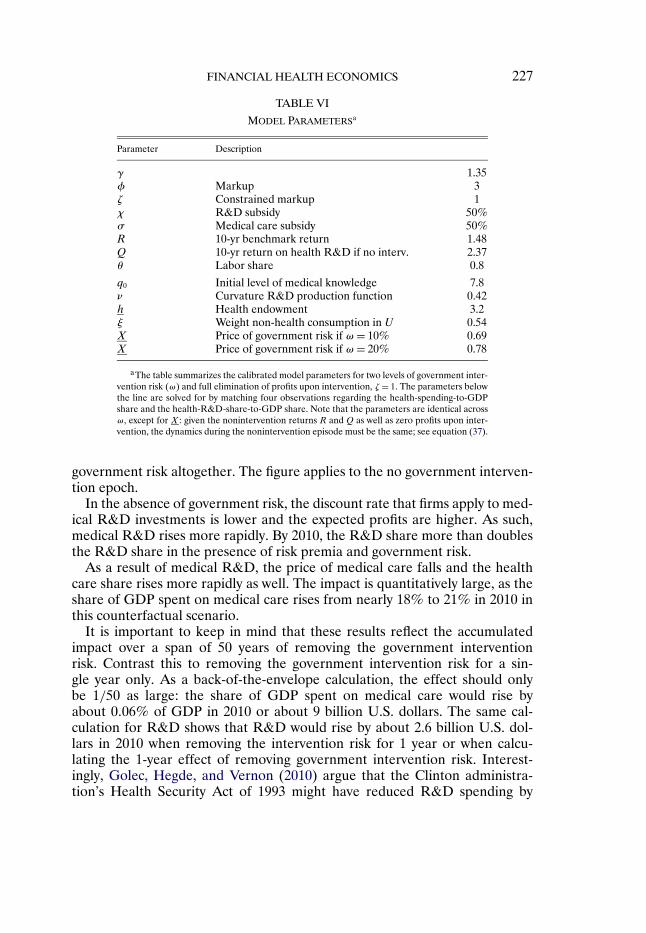
FINANCIAL HEALTH ECONOMICS 227
TABLE VI
MODEL PARAMETERSa
Parameter Description
γ 1.35φ Markup 3ζ Constrained markup 1χ R&D subsidy 50%σ Medical care subsidy 50%R 10-yr benchmark return 1.48Q 10-yr return on health R&D if no interv. 2.37θ Labor share 0.8
q0 Initial level of medical knowledge 7.8ν Curvature R&D production function 0.42h Health endowment 3.2ξ Weight non-health consumption in U 0.54X Price of government risk if ω= 10% 0.69X Price of government risk if ω= 20% 0.78
aThe table summarizes the calibrated model parameters for two levels of government inter-vention risk (ω) and full elimination of profits upon intervention, ζ = 1. The parameters belowthe line are solved for by matching four observations regarding the health-spending-to-GDPshare and the health-R&D-share-to-GDP share. Note that the parameters are identical acrossω, except for X : given the nonintervention returns R and Q as well as zero profits upon inter-vention, the dynamics during the nonintervention episode must be the same; see equation (37).
government risk altogether. The figure applies to the no government interven-tion epoch.
In the absence of government risk, the discount rate that firms apply to med-ical R&D investments is lower and the expected profits are higher. As such,medical R&D rises more rapidly. By 2010, the R&D share more than doublesthe R&D share in the presence of risk premia and government risk.
As a result of medical R&D, the price of medical care falls and the healthcare share rises more rapidly as well. The impact is quantitatively large, as theshare of GDP spent on medical care rises from nearly 18% to 21% in 2010 inthis counterfactual scenario.
It is important to keep in mind that these results reflect the accumulatedimpact over a span of 50 years of removing the government interventionrisk. Contrast this to removing the government intervention risk for a sin-gle year only. As a back-of-the-envelope calculation, the effect should onlybe 1/50 as large: the share of GDP spent on medical care would rise byabout 0�06% of GDP in 2010 or about 9 billion U.S. dollars. The same cal-culation for R&D shows that R&D would rise by about 2.6 billion U.S. dol-lars in 2010 when removing the intervention risk for 1 year or when calcu-lating the 1-year effect of removing government intervention risk. Interest-ingly, Golec, Hegde, and Vernon (2010) argue that the Clinton administra-tion’s Health Security Act of 1993 might have reduced R&D spending by

228 R. S. J. KOIJEN, T. J. PHILIPSON, AND H. UHLIG
FIGURE 3.—Health and R&D share in the model and in the data.
about 1 billion U.S. dollars, as a “conservative” estimate, “even though itnever became law.” Our R&D measure for the sector is more inclusive andabout twice as large as theirs. Furthermore, they essentially examined the im-pact of an increased probability of some government intervention, whereasour number pertains to the full effect of overall government intervention. Wetherefore view our quantitative implications as broadly in line with their find-ings.
6.2.2. Second Counterfactual: No Government Risk Premium
As a second counterfactual, we consider the case in which the governmentrisk is present (ω= 10% or ω= 20%), but we set the price of government in-tervention risk to zero, X =X = 1. This case corresponds to the two middle(dashed–dotted and dotted) lines in Figure 4. This case allows us to understandtwo effects that are in play in the first counterfactual separately. More pre-cisely, if all government risk is removed, then Et[πt+1] increases and the priceof this cash flow, Et[Mt+1πt+1], increases as well. We are particularly interestedin the effect of risk premia on medical innovation and spending; therefore, wewant to hold constant the impact on expected profits, Et[πt+1].
Based on Figure 4, we see that removing the risk premium alone accountsfor three-quarters of the increase in the health care share and R&D share

FINANCIAL HEALTH ECONOMICS 229
FIGURE 4.—Counterfactual dynamics of health care and R&D spending.
for ω = 10%, and is responsible for about half of it at ω = 20%. This com-pares well to the following back-of-the-envelope calculation. A per-decade in-tervention risk of 20% yields an annual intervention risk of about 2%. Withan annual risk premium of 5%, about 3% of that must then be due to the riskpremium against this intervention. We have argued above that ω= 20% is anupper bound for a reasonable intervention probability. We conclude that therisk premium as compared to the actuarially fair disaster premium is the moreimportant component for explaining the “missing R&D” compared to the non-intervention scenario, as well as the financial health premium for investors inthat sector. Table VII provides a numerical summary of our results.
6.3. Long-Run Implications
Absent government intervention, the long-run health care share implied bythe model is ψ∞ (see equation (25)), which equals 32% in the presence of sub-sidies. If subsidies in the output market are removed, that is, σ = 0, the sharedecreases to 25%. Note that the shares differ from 1 − ξ, since the profits ofthe health sector are counted as part of GDP and, thus, in this ratio. Figure 5illustrates the evolution of the health care spending share and the R&D shareas implied by the model, provided no government intervention takes place and

230 R. S. J. KOIJEN, T. J. PHILIPSON, AND H. UHLIG
TABLE VII
HEALTH AND R&D SHARE DYNAMICS FOR BOTHCOUNTERFACTUALS AND DIFFERENT LEVELS OF GOVERNMENT RISKa
Benchmark: No Government Risk No Government Risk No GovernmentBenchmark: Premium, ω= 20% Premium, ω= 10% Risk
Health share1960 5�1% 5�1% 5�1% 5�1%1970 6�8% 7�1% 7�3% 7�5%1980 8�9% 9�7% 10�2% 10�6%1990 11�6% 12�9% 13�6% 14�2%2000 14�7% 16�3% 17�1% 17�9%2010 17�9% 19�6% 20�5% 21�2%
R&D share1960 0�1% 0�1% 0�1% 0�1%1970 0�1% 0�2% 0�2% 0�3%1980 0�2% 0�3% 0�4% 0�6%1990 0�3% 0�6% 0�7% 0�9%2000 0�5% 0�8% 1�0% 1�3%2010 0�7% 1�1% 1�4% 1�6%
aThe table illustrates the impact of government risk and the medical innovation premium on health care and R&Dspending. The second column provides the benchmark results, the third column removes government risk altogether,and the fourth column considers the counterfactual in which there is government risk, but this risk is not priced inequilibrium.
comparing the benchmark with the three counterfactuals. Obviously, the con-vergence is rather slow and the health care share is expected to increase to30% by 2050. This prediction is similar to the model of Hall and Jones (2007).While the limit for the health spending share without government interventionis independent of ω, given Q, this is not true for the R&D share: indeed, with-out government intervention risk, it converges to about 2.5% of GDP ratherthan 1.6% of GDP.
Once the government intervenes, R&D activity will come to a halt if left toprivate markets. The R&D share drops to zero and the gross income share λtspent on medical care jumps, but then remains constant, as explained belowequation (21).
6.4. R&D With Fixed Costs, Idiosyncratic Risk, and Heterogeneity
In our model, the only source of aggregate risk is the government interven-tion risk.17 Furthermore, R&D success is a smooth, nonprobabilistic functionof R&D effort and there is no heterogeneity across firms in equilibrium. While
17As noted in Section 6.1, we calibrate the nonintervention return to be 4% rather than thesafe rate of 1% to account for the fact that there are other aggregate risks, which demand a riskpremium in equilibrium and, therefore, lower medical R&D.

FINANCIAL HEALTH ECONOMICS 231
FIGURE 5.—Model-implied long-run dynamics of the health and R&D share.
these are useful assumptions in the service of the simplicity of the model, it isuseful to understand whether our results carry over to a more general specifi-cation and under what conditions, as one may regard a richer set of possibil-ities here as important for understanding medical R&D and the competitionin the health industry. The purpose of this section is to clarify how the resultsreported thus far can be generalized.
Consider qualities qjt and prices pjt for all firms j ∈ [0�1]. As usual in mo-nopolistic competition models, define
qt =(∫ 1
0q1/(φ−1)jt dj
)φ−1
� pt =(∫ 1
0p1/(1−φ)jt dj
)1−φ�(40)
dt =∫ 1
0djt dj�
where we allow for stochastic variations across j ∈ [0�1], including idiosyncraticrisk: in that case, the integrals should be understood as Pettis integrals; seeUhlig (1996). The aggregate equilibrium dynamics in the model remains thesame, if the dynamics of the aggregators qt , pt , and dt remain the same. Thisthen is the property that needs verification if additional features are added.

232 R. S. J. KOIJEN, T. J. PHILIPSON, AND H. UHLIG
Given the markup pricing, the dynamics for pt is implied by the dynamics forqt ; hence, it remains to verify the dynamics for qt and dt .
Consider now some more general model specification, including idiosyn-cratic risk and firm heterogeneity. Assume first that entrepreneurs cross-insureeach other. That is, while each pursues the objective of profit maximization forthe firm managed by that individual entrepreneur, share holdings in the healthindustry are diversified across entrepreneurs, idiosyncratic risk is washed outin their portfolio, and the stochastic discount factor depends on aggregate riskonly. Examine a generalized version of the firm maximization problem statedjust before (26), allowing for a firm-specific starting quality q̃jt as well as a po-tentially random outcome for qj�t+1:
v(djt� q̃jt)= maxdjt
(Et
[Mt+1πt+1
q1/(φ−1)t+1
])Et
[q1/(φ−1)j�t+1
] − (1 −χ)djt(41)
s.t. qj�t+1 = f (djt� q̃jt�μj�t+1)
for some random variable μj�t+1, idiosyncratic and identically distributed acrossj and t, and some suitable function f (·� ·� ·). With this notation, we allow thestarting point q̃j�t+1 in t + 1 to be different from qj�t+1: for the aggregate dy-namics, we then need to clarify the relationship between the two. We assumedate-t-conditional independence of the random idiosyncratic outcome μj�t+1
from the aggregate variables Mt+1, πt+1, and qt+1. This independence betweenidiosyncratic and aggregate risk allows us to separate the expectations of thefirm-individual piece and the aggregate piece above.
Suppose now that
Et[q1/(φ−1)j�t+1
] = (q̃νjt + dνjt
)1/((φ−1)ν)(42)
locally around the equilibrium choice djt =Dt(q̃jt) of the model above, for anyinitial q̃jt . Note that this property is satisfied in the absence of idiosyncratic risk(see equation (11)) and, therefore, is consistent with the baseline version of themodel. With (42), the first-order condition for djt in (42) around that equilib-rium choice remains unchanged. If it also characterizes the global maximum,then the choice for djt remains unchanged, given q̃jt . This includes several in-teresting special cases.
One case, without idiosyncratic risk, is a nonbinding fixed cost for R&D asan alternative to (11) for the specification of f (·� ·� ·). Say
q̃j�t+1 = qj�t+1 = 1djt>0�9Dt(q̃jt )
(q̃νjt + dνjt
)1/ν�
where 1djt>0�9Dt(q̃jt ) indicates that the next-period quality qj�t+1 will be zero un-less R&D efforts djt exceed the threshold of 90% of the equilibrium choiceDt(q̃jt). Furthermore, given the same starting point q̃j0 ≡ q0 at date 0 for allfirms, a symmetric equilibrium qjt ≡ qt , djt = dt will persist. Obviously, the

FINANCIAL HEALTH ECONOMICS 233
equilibrium dynamics changes with a threshold that binds in equilibrium orother initial conditions: our aim here is simply to show that there are versionsof our model that include fixed costs and that nonetheless give rise to the samedynamics.
For the easiest cases involving idiosyncratic risk, assume an R&D externalityto hold across all firms: while qj�t+1 = f (djt� q̃jt�μj�t+1) is the profit-relevantnext-period quality for the date-t investing firm and, thus, is relevant for thefirm problem (41) stated above, assume that new firms j in date t + 1 all startfrom the same quality level q̃j�t+1, which is possibly different from qj�t+1. Moreprecisely, assume that all firms start from
q̃jt = qt(43)
for every period t, where qt is given by the quality average in (40). Assume that(42) holds and that the starting point q0 here is the same as in the baselinemodel. By induction, we shall show that we obtain the same aggregate equi-librium as in the baseline model. Assume, that qt here and given by (40) atsome given date t coincides with qt of the baseline model. With (43), the R&Defforts djt = dt are then the same across all firms and coincide with dt of thebaseline model. Comparing (11) to (42), it follows that Et[q1/(φ−1)
j�t+1 ] coincideswith q1/(φ−1)
t+1 of the baseline model. Equation (40) then shows that
qt+1 = (Et
[q1/(φ−1)j�t+1
])φ−1
here must coincide with qt+1 of the baseline model as well, completing theinduction argument.
The easiest way to guarantee (42) is to perturb the R&D outcome (11) withan exogenous and idiosyncratic factor μj�t+1 ≥ 0,
qj�t+1 = f (djt� q̃jt�μj�t+1)= μj�t+1
(q̃νjt + dνjt
)1/ν�(44)
where
1 =Et[μ1/(φ−1)j�t+1
]�(45)
As a particular example, one might wish to assume that μj�t+1 = αφ−1 with someprobability 0<α< 1 and μj�t+1 = 0 with probability 1 − α, idiosyncratic acrossj and t, capturing the idea that medical R&D succeeds only occasionally. Withthe assumption (43) of the R&D externality across all firms and, thus, q̃jt ≡ qt ,djt ≡ dt , one obtains the previously calculated equilibrium. It is straightforwardto generalize this result to a richer set of specification, where the probabilitydistribution of R&D or the probability of R&D success actually depends onR&D effort without changing the resulting equilibrium. The key is to “split”the extensive or probabilistic dimension from the intensive or quality-level di-mension in such a way that (45) continues to hold.

234 R. S. J. KOIJEN, T. J. PHILIPSON, AND H. UHLIG
Matters become more involved, once one allows heterogeneity across firmsand persistence in the R&D outcome, dispensing with the R&D-externality-across-all-firms assumption and replacing it with the assumption that
q̃j�t+1 = qj�t+1 = f (djt� qjt�μj�t+1)�
The calculations and required functional choices for obtaining the same dy-namics still remain reasonably tractable if one assumes that φ = 2. One canthen rewrite (42) as
Et
[qj�t+1
qjt
]=
(1 +
(djt
qjt
)ν)1/ν
�(46)
As an example, assume the specification of a random multiplicative distur-bance (44), imposing
1 =E[μjt]�
which coincides with (45) due to φ= 2. One can now see that proportionality
djt
qjt= dt
qt
satisfies (46) as well as (40) and, thus, provides the equilibrium with the sameaggregate dynamics as before. Note that there is considerable and persistentheterogeneity across firms in this case.
Building on these insights, and at the cost of further algebra and unwieldyfunctional form specifications, it appears to be possible to combine the featuresof the cases above, allow for φ = 2, and introduce correlated risks as well. Thismay be an interesting research project to pursue so as to study the dynamicsof the industrial organization of the health industry or other industries, but isbeyond the scope of this paper.
With the kinked-linear utility specification for the entrepreneur, it further-more is not hard to calculate the dynamics of the model if there is no portfoliodiversification and insurance across entrepreneurs. In that case, the risk pre-mium arises due to idiosyncratic risks as well as aggregate risks, and one needsadditional analysis to disentangle the two. We find this to be a less attractivespecification for the model, since it seems a priori more plausible that investorshold a somewhat diversified portfolio and will be particularly enticed to do soif risk premia are due entirely or to a large extent to idiosyncratic risk. We donot find it plausible that such a risk premium could persist over the long spanof time, as we have observed in the health industry.

FINANCIAL HEALTH ECONOMICS 235
7. RELATED LITERATURE AND MECHANISMS FOR HEALTH CARE RISK PREMIA
7.1. Related Literature
Our paper relates to several strands of previous research by merging insightfrom three separate fields: health economics, macroeconomics, and finance.Therefore, we briefly review how our work relates to some key papers in allthree fields. Our paper differs from previous works by examining the joint de-termination of financial asset returns for those investing in medical innovationand the resulting growth in the real health care sector.
Our paper adds the analysis of R&D incentives to the macroeconomic lit-erature, which has analyzed the relationship between health and growth; see,for instance, Barro (1996) and Sala-i-Martin, Doppelhofer, and Miller (2004).A large empirical literature in health economics estimates the impact of eco-nomic growth on health care spending; see Gerdtham and Jonsson (2000) fora review.
A seminal paper analyzing the interrelationship between macroeconomicgrowth and the share of income spent on health is Hall and Jones (2007). Theseauthors point out that a rise in the share is predicted by many reasonable pref-erence specifications, as the value of additional health spending increases rel-ative to consumption when the marginal utility for extra consumption declineswith growth. Hall and Jones (2007) provide a detailed quantitative analysis ofthe effect and social desirability of health spending.18
We view our paper as complementary to theirs. In particular, our focus ison the innovation in the health sector and the entrepreneurial risks associ-ated with that investment, while these authors assume technological progressin the health sector to be deterministic and exogenous. While the long-run de-mand for new innovations in health might well be due to the forces Hall andJones (2007) discuss, the key entrepreneurial risks arise from the possibility ofgovernmental intervention rather than, say, risks in the effectiveness of healthspending in increasing longevity, as we discuss in Section 7. Compared to theirmodel, our model puts the incentives for R&D at center stage, which requiresus to extend the model along this dimension, while simplifying the longevityanalysis performed by Hall and Jones (2007).
In finance, our paper relates to recent literature that shows that governmentrisk affects asset prices.19 The main contribution of our paper is to document
18The empirical evidence showing that health care is a luxury good is mixed; see Acemoglu,Finkelstein, and Notowidigdo (2009) and the references therein. Also, in the cross section, healthcare is a necessity in the upper part of the income distribution, suggesting that technology mayultimately be the barrier to rich people from spending larger shares of their incomes on healthcare.
19For instance, Belo, Gala, and Li (2013) link the cross section of expected stock returns tofirms’ exposures to the government sector. Brogaard and Detzel (2013) use the political uncer-tainty index of Baker, Bloom, and Davis (2013) to show that spikes in political uncertainty gotogether with declines in the stock market, which is largely the result of increases in risk premia.

236 R. S. J. KOIJEN, T. J. PHILIPSON, AND H. UHLIG
the medical innovation premium in the health care sector and to map out theimplications for investment in medical R&D and, thus, future health care ex-penditures. As a potential explanation of this risk premium, we point to therisk of government intervention.
Most closely related to our paper are Ellison and Mullin (2001) and Golec,Hegde, and Vernon (2010), who study the impact of the Clinton health carereform proposals in 1992 and 1993 on stock prices. Both papers find that healthcare stocks are negatively impacted by the Clinton reform plans. Furthermore,Golec, Hegde, and Vernon (2010) also show that the effect is more pronouncedfor R&D intensive firms and that (unexpected) R&D declines more for thosefirms that are more exposed to government intervention risk.20 This evidenceis consistent with the main implications of our model.
7.2. Broad Intuition for Alternative Mechanisms
In this section, we discuss qualitatively and in an exploratory fashion variouseconomic mechanisms that may give rise to the medical innovation premium.This boils down to understanding how certain shocks, in general equilibrium,co-move with the investors’ marginal utility. This section uses a broad theorybrush, focusing on the key economic arguments and without providing a com-prehensive list of assumptions and caveats. We first provide a broader overviewand then examine some approaches in somewhat more careful detail.
The key finding from the empirical results is the medical innovation pre-mium, which implies that ∂U/∂ct+1 is low when health industry profits πt+1 arehigh. Ceteris paribus, marginal utility is low if consumption is high.
To analyze other factors that may yield the medical innovation premium,consider a representative household that demands medical care m, resultingin health h=m. Medical care can be provided with productivity (or “quality,”“inverse of marginal costs”) q and sold at price p, while subsidized at rate σ .The subsidies are financed per lump-sum taxes τ on the household. Assume alinear production function and denote the markup with φ. Profits of the med-ical sector are π. Aggregate income is y , while aggregate consumption is c.Preferences by the household are given by a utility function u(c�h).
For a linear production function, the relationship between prices, marginalcosts, mark-ups, and profits are
p= φ
qand π = (φ− 1)
h
q�(47)
Kelly, Pastor, and Veronesi (2014) show how political uncertainty is priced in the option marketusing national elections and global summits, building on the theories developed in Pastor andVeronesi (2011) and Pastor and Veronesi (2016). These papers do not focus on the health caresector.
20Julio and Yook (2012) show more generally how corporate investment is affected negativelyby political uncertainty.

FINANCIAL HEALTH ECONOMICS 237
The household budget constraint is
y +π = c+ (1 − σ)ph+ τ�(48)
The government budget constraint is
σph= τ�(49)
Together, we obtain the two key equations
c = y − h/q= y −π/(φ− 1)�(50)
π = (φ− 1)h/q�(51)
These equations imply that approaches that treat y , φ, and q as parameters orconstants are challenging to pursue. Consider the following sources of uncer-tainty:
1. Medical progress, including longevity: If q increases, so will h. See Sec-tion 7.3 for further details.
2. Preference shocks for h, with c and h separable or complements in theutility function u(·� ·).
3. A shock to the subsidies σ .The challenge is the following. Suppose that these shocks result in surpriseincreases in profits π. They will then lead to lower consumption. Conversely,lower profits go together with higher consumption. In the cases above, thisshould yield a negative, not a positive alpha.
Approaches that treat all of π, h, c, y , φ, and q as endogenous have morepotential to be successful. Consider the following sources of uncertainty:
1. Medical progress and productivity. Suppose a surprise increase in q leadsto a more productive workforce, thereby increasing y . It is then possible, inprinciple, to have both π and c increase.
2. A preference shock for h, where c and h are (strong) substitutes in theutility function u(·� ·). Suppose that h is increased and thus profits π increase,while consumption c decreases. In principle, it is nonetheless possible that themarginal utility of consumption decreases as well.
3. Government regulatory risk regardingφ: ifφ declines unexpectedly, thenso will π and c, while h increases.These approaches face challenges on their own. The first one may not besufficient quantitatively: while medical progress has perhaps led to somewhatlonger working life and to fewer absentee hours due to sickness in the UnitedStates after the Second World War, these effects may be too small to sensiblygenerate the medical innovation premium that we estimate in our empiricalwork. The second approach may not be plausible. Per our own introspection, itdoes seem to us that consumption and marginal increases thereof are more fun

238 R. S. J. KOIJEN, T. J. PHILIPSON, AND H. UHLIG
and not less fun if one is healthy.21 We, therefore, chose the third approach asthe key approach in this paper. The arguments above are painted with a broadbrush: it is entirely conceivable, even plausible, that reasonable exceptions canbe found that allow the pursuit of other alternatives. For some of them, moredetail is useful to reveal where the challenges lie exactly. We shall do so, inparticular, for longevity risk.
7.3. Risk Premia due to Longevity Effects
Longevity is the key to understanding the growth of health expenditures inthe model of Hall and Jones (2007). Our paper is not in contrast to theirs;rather, it is complementary. While longevity may indeed be key (and indeed,our long-run improvements in health may well be interpreted as increases inlongevity), we argue here that they are unlikely to be the risk factor giving riseto the medical innovation premium.
Consider a three-period extension of the model above, t = 0�1�2, where thehousehold surely survives until t = 1. The probability of survival from t = 1 tot = 2 depends on health, f (h1), where f ′(h1) > 0. The household’s problemcan then be summarized by
max(h1)
u(c0)+βE0
[u(c1)
] +β2E0
[f (h1)u(c2)
]�(52)
where the maximization is subject to the resource constraints, yt +πt = ptht +ct , the prices of medical care, pt =φt/qt , and firm profits, πt = ht(φt −1)/qt .22
Unless noted otherwise, we focus on shocks to qt that lower the marginal costof producing medical care.
Optimal period-1 health follows from max(h1) u(c1) + f (h1)b, where b =βE1[u(c2)] > 0 a constant. In this case, we have c1 = y1 − h1q
−11 = y1 − (φ1 −
1)−1π1, which implies that consumption and profits are negatively correlated.Since M1 = βu′(c1)/u
′(c0) = βu′(y1 − (φ1 − 1)−1π1)/u′(c0), profits and the
stochastic discount factor are positively correlated. This implies a negative riskpremium for health care firms. This holds true regardless of the survival func-tion f (h1) and as long as u′(c) < 0.
8. CONCLUSION
Despite the fact that improvements in health care and health have been ma-jor components of the overall gain in economic welfare during the last cen-tury, the continued financial incentives for medical innovation and the result-ing growth of the health care sector are not well understood. Although it is
21This is also consistent with the empirical results in Viscusi and Evans (1990), Finkelstein,Luttmer, and Notowidigdo (2008), and Koijen, Van Nieuwerburgh, and Yogo (2011).
22Relative to our full model, we consider a simpler production for health with h= 0 and ν = 1,which implies that medical spending maps one-to-one to health, mt = ht .

FINANCIAL HEALTH ECONOMICS 239
generally believed that medical innovation and its demand are central compo-nents of the expansion of this sector, little is known about what risks affect thereturns of R&D investments and how those risks, in turn, affect future spend-ing growth.
We provided an empirical and theoretical analysis of the link between finan-cial and real health care markets. We first documented a “medical innovationpremium” for the returns of medical R&D firms in the United States duringthe period from 1960 to 2010 and provided suggestive evidence of governmentintervention risk as a determinant of this premium. The excess returns relativeto standard risk adjustments were estimated to be 4–6% per annum, which islarge and about the same size as other asset pricing puzzles, such as the eq-uity risk premium and the value premium during this period. Motivated bythis finding, we provided a theoretical analysis of the joint determination offinancial and real health care markets. We interpreted the medical innovationpremium to result from government markup risks that might require investorsto demand higher returns on medical R&D investments beyond standard risk-adjusted returns.
We simulated the quantitative implications of the medical innovation pre-mium on health care spending and on spending growth on medical R&D. Wefound that there would have been a sizeable expansion of the health care sectorby 3% of GDP, as well as more than a doubling of R&D efforts, in the absenceof government risk, holding back innovation. The difference is due to an ac-tuarially fair disaster premium as well as a risk premium against that disaster.We found that the risk premium is the larger component.
Our analysis raises many future questions that need to be addressed to morefully understand the growth of health care sectors around the world. First, ifgovernment uncertainty discourages health care R&D, then how are standardanalyses of government interventions altered by taking into account this ef-fect? For example, most governments across the world attempt to stimulatemedical R&D through various push-and-pull mechanisms. But if the govern-ment uncertainty attached to such mechanisms discourages R&D, how muchdoes this uncertainty reduce the intended effects of such R&D stimuli? Sec-ond, discounting future public health care liabilities by U.S. Treasury rates, asis done for future Medicare liabilities by the CBO, rather than how marketsdiscount health care spending, seems inappropriate in light of the medical in-novation premium documented in this paper.23 Third, many policy proposalsto slow spending growth in health care need to incorporate the governmentrisk and its effect on medical R&D. For example, the 2010 report of the Na-tional Commission on Fiscal Responsibility and Reform suggests imposing re-strictions on publicly financed health care spending tied to GDP growth. Our
23See Geanakoplos and Zeldes (2011) and Lucas (2010) for recent work on the valuation ofgovernment liabilities.

240 R. S. J. KOIJEN, T. J. PHILIPSON, AND H. UHLIG
framework and analysis can be used to consider imposing government restric-tions on health care spending and to quantify their effects, including the growtheffects introduced by policy uncertainty of implementing the restrictions them-selves.
More generally, we believe future analyses need to better incorporate theinteraction between financial markets that affect R&D investments, govern-ment risk, and the resulting growth of the health care sector. The growth of thehealth care sector depends on medical R&D, which is affected by governmentrisk, which in turn means that greater uncertainty introduced by governmentintervention discourages medical R&D. This important feedback mechanismimplies that any future growth of government programs, such as, for instance,Medicare, is tied to the risk of policies surrounding those programs. Overall,we believe that further explicit analyses of the dynamic incentives for contin-ued medical progress are warranted given the dramatic effects such progresshas on overall health care spending and health. Overall, we believe that fur-ther explicit analyses of the interaction between real and financial healthcaremarkets are warranted given the dramatic effects medical R&D has on overallhealthcare spending and health.
REFERENCES
ACEMOGLU, D., A. FINKELSTEIN, AND M. J. NOTOWIDIGDO (2009): “Income and Health Spend-ing: Evidence From Oil Price Shocks,” Working Paper, MIT. [235]
BAKER, S. R., N. BLOOM, AND S. J. DAVIS (2013): “Measuring Economic Policy Uncertainty,”Working Paper, Stanford University. [235]
BARRO, R. J. (1996): “Health and Economic Growth,” Working Paper, Harvard University. [235]BARRO, R. J., AND T. JIN (2011): “On the Size Distribution of Macroeconomic Disasters,” Econo-
metrica, 79 (5), 1567–1589. [197]BARRO, R. J., AND J. F. URSUA (2008): “Consumption Disasters in the Twentieth Century,” Amer-
ican Economic Review, 98 (2), 58–63. [197]BECKER, G. S., T. PHILIPSON, AND R. R. SOARES (2005): “The Quantity and Quality of Life and
the Evolution of World Inequality,” American Economic Review, 95, 277–291. [195]BELO, F., V. GALA, AND J. LI (2013): “Government Spending, Political Cycles and the Cross
Section of Stock Returns,” Journal of Financial Economics, 107, 305–324. [235]BERK, J. B., R. C. GREEN, AND V. NAIK (1999): “Optimal Investment, Growth Options and
Security Returns,” Journal of Finance, 54, 1153–1607. [200]BROGAARD, J., AND A. L. DETZEL (2013): “The Asset Pricing Implications of Government Eco-
nomic Policy Uncertainty,” Working Paper, University of Washington. [235]CAMPBELL, J. Y., A. W. LO, AND A. C. MACKINLAY (1997): The Econometrics of Financial Mar-
kets. Princeton, NJ: Princeton University Press. [209]CAVES, R. E., M. D. WHINSTON, AND M. A. HURWITZ (1991): “Patent Expiration, Entry, and
Competition in the U.S. Pharmaceutical Industry,” Brookings Papers on Economic Activity, Mi-croeconomics, June 20, 1–66. [225]
CUTLER, D. M. (1995): “Technology, Health Costs, and the NIH,” Working Paper, Harvard Uni-versity. [196]
EGAN, M., AND T. PHILIPSON (2013): “International Health Economics,” Working Paper 19280,NBER. [198]
ELLISON, S. F., AND W. P. MULLIN (2001): “Gradual Incorporation of Information: Pharmaceuti-cal Stocks and the Evolution of President Clinton’s Health Care Reform,” Journal of Law andEconomics, 34, 89–129. [196,208,236]

FINANCIAL HEALTH ECONOMICS 241
FAMA, E. F., AND K. R. FRENCH (1992): “The Cross-Section of Expected Returns,” Journal ofFinance, 47, 427–465. [196,199,200,202]
(1997): “Industry Costs of Equity,” Journal of Financial Economics, 43, 153–193. [202]FENG LI, R. L., AND M. MINNIS (2013): “A Measure of Competition Based on 10-K Filings,”
Journal of Accounting Research, 51, 399–436. [202]FINKELSTEIN, A., E. F. P. LUTTMER, AND M. J. NOTOWIDIGDO (2008): “What Good Is Wealth
Without Health? The Effect of Health on the Marginal Utility of Consumption,” WorkingPaper, MIT. [212,238]
FUCHS, V. (1996): “Economics, Values, and Health Care Reform,” American Economic Review,86, 1–24. [196]
GABAIX, X. (2012): “Variable Rare Disasters: An Exactly Solved Framework for Ten Puzzles inMacro-Finance,” Quarterly Journal of Economics, 127 (2), 645–700. [197]
GEANAKOPLOS, J., AND S. P. ZELDES (2011): “The Market Value of Social Security,” WorkingPaper, Yale University. [239]
GERDTHAM, U.-G., AND B. JONSSON (2000): “International Comparisons of Health Expenditure:Theory, Data and Econometric Analysis,” in Handbook of Health Economics, Vol. 1. Amster-dam: North-Holland/Elsevier, 11–53. [235]
GOLEC, J. H., S. HEGDE, AND J. VERNON (2010): “Pharmaceutical R&D Spending and Threatsof Price Regulation,” Journal of Financial and Quantitative Analysis, 45, 239–264. [196,208,209,
227,236]GROSSMAN, S. J., AND Z. ZHOU (1993): “Optimal Investment Strategies for Controlling Draw-
downs,” Mathematical Finance, 3, 241–276. [205]HALL, R. E., AND C. I. JONES (2007): “The Value of Life and the Rise in Health Spending,”
Quarterly Journal of Economics, 122, 39–72. [213,230,235,238]HOBERG, G., AND G. PHILLIPS (2011): “Text-Based Network Industries and Endogenous Product
Market Differentiation,” Working Paper, University of Maryland. [202]HULT, K. J., AND T. J. PHILIPSON (2012): “Public Liabilities and Health Care Policy,” Working
Paper 18571, National Bureau of Economic Research. [206]JONES, C. I. (2011): “Life and Growth,” Working Paper, Stanford University. [225,226]JULIO, B., AND Y. YOOK (2012): “Political Uncertainty and Corporate Investment Cycles,” Jour-
nal of Finance, 67, 45–83. [236]KAHNEMAN, D., AND A. TVERSKY (1979): “Prospect Theory: An Analysis of Decisions Under
Risk,” Econometrica, 47 (2), 263–292. [212]KELLY, B. T., L. PASTOR, AND P. VERONESI (2014): “The Price of Political Uncertainty: Theory
and Evidence From the Option Market,” Working Paper, University of Chicago. [236]KOGAN, S., D. LEVIN, B. ROUTLEDGE, J. SAGI, AND N. SMITH (2009): “Predicting Risk From
Financial Reports With Regression,” Proceedings of the North American Association for Com-putational Linguistics Human Language Technologies Conference. [202]
KOIJEN, R. J., T. J. PHILIPSON, AND H. UHLIG (2016): “Supplement to ‘Financial Health Eco-nomics’,” Econometrica Supplemental Material, 84, http://dx.doi.org/10.3982/ECTA11182. [202]
KOIJEN, R. S., S. VAN NIEUWERBURGH, AND M. YOGO (2011): “Health and Mortality Delta:Assessing the Welfare Cost of Household Insurance Choice,” Working Paper, University ofChicago. [212,238]
KOIJEN, R. S. J., H. LUSTIG, AND S. VAN NIEUWERBURGH (2012): “The Cross-Section and TimeSeries of Stock and Bond Returns,” Working Paper. [200]
KOIJEN, R. S. J., T. J. MOSKOWITZ, L. H. PEDERSEN, AND E. B. VRUGT (2013): “Carry,” WorkingPaper, Business School. [205]
LANDONI, M., AND R. SASTRY (2013): “Quantifying Tail Risk in Hedge Funds,” Working Paper,Columbia Business School. [205]
LETTAU, M., AND J. A. WACHTER (2007): “Why Is Long-Horizon Equity Less Risky? A Duration-Based Explanation of the Value Premium,” Journal of Finance, 62, 55–92. [200]
LOUGHRAN, T., AND B. MCDONALD (2011): “When Is a Liability not a Liability? Textual Analysis,Dictionaries, and 10-Ks,” Journal of Finance, 66, 35–65. [202]

242 R. S. J. KOIJEN, T. J. PHILIPSON, AND H. UHLIG
LUCAS, D. E. (2010): Measuring and Managing Federal Financial Risk. Chicago: University ofChicago Press. [239]
MCGRATTAN, E. R., AND E. C. PRESCOTT (2003): “Average Debt and Equity Returns: Puzzling?”American Economic Review, 93 (2), 392–397. [225]
MURPHY, K. M., AND R. H. TOPEL (2006): “The Value of Health and Longevity,” Journal ofPolitical Economy, 114, 871–904. [195,197]
NEWHOUSE, J. P. (1992): “Medical Care Costs: How Much Welfare Loss?” Journal of EconomicPerspectives, 6, 3–21. [196]
PASTOR, L., AND P. VERONESI (2011): “Political Uncertainty and Risk Premia,” Working Paper.[236]
(2016): “Uncertainty About Government Policy and Stock Prices,” Journal of Finance(forthcoming). [236]
SALA-I-MARTIN, X. X., G. DOPPELHOFER, AND R. I. MILLER (2004): “Determinants of Long-Term Growth: A Bayesian Averaging of Classical Estimates (BACE) Approach,” AmericanEconomic Review, 94, 813–835. [235]
SHARPE, W. (1964): “Capital Asset Prices: A Theory of Market Equilibrium Under Conditions ofRisk,” Journal of Finance, 19, 425–444. [196,199]
UHLIG, H. (1996): “A law of Large Numbers for Large Economies,” Economic Theory, 8, 41–50.[231]
VISCUSI, K. W., AND W. N. EVANS (1990): “Utility Functions That Depend on Health Status:Estimates and Economic Implications,” American Economic Review, 80, 353–374. [212,238]
YOGO, M. (2006): “A Consumption-Based Explanation of the Cross Section of Expected StockReturns,” Journal of Finance, 61 (2), 539–580. [200]
ZHANG, L. (2005): “The Value Premium,” Journal of Finance, 60, 67–103. [200]
London Business School, Regent’s Park, London, NW1 4SA, U.K.; [email protected],
Irving B. Harris Graduate School of Public Policy, University of Chicago, Suite112, 1155 E. 60th Street, Chicago, IL 60637, U.S.A.; [email protected],
andDept. of Economics, University of Chicago, RO 325A, 1126 East 59th Street,
Chicago, IL 60637, U.S.A.; [email protected].
Manuscript received October, 2012; final revision received June, 2015.


