Financial frictions in Latvia -...

Noname manuscript No.(will be inserted by the editor)

Financial frictions in Latvia

Ginters Buss

Received: date / Accepted: date

Abstract This paper builds a dynamic stochastic general equilibrium (DSGE) model for Latvia thatwould be suitable for policy analysis and forecasting purposes at Bank of Latvia. For that purpose, Iadapt the DSGE model with financial frictions of Christiano, Trabandt and Walentin (2011, “Introducingfinancial frictions and unemployment into a small open economy model” in Journal of Economic Dynamicsand Control) to Latvia’s data, estimate it, and study whether adding the financial frictions block to anotherwise identical (‘baseline’) model is an improvement with respect to several dimensions. The mainfindings are: i) the addition of the financial frictions block provides more appealing interpretation for thedrivers of economic activity, and allows to reinterpret their role; ii) financial frictions played an importantpart in Latvia’s 2008-recession; iii) the financial frictions model beats both the baseline model and therandom walk model in forecasting both CPI inflation and GDP.

Keywords DSGE model · Financial frictions · Small open economy · Bayesian estimation · Currencyunion

JEL codes E0, E3, F0, F4, G0, G1

Disclaimer: The views expressed in this paper are those of the author and do not necessarily reflect the views of the Bankof Latvia.

G. BussBank of Latvia, K. Valdemara 2A, Riga, LV-1050, LatviaTel.: +371-25-529117Fax: +371-67-022420E-mail: [email protected]

1 Introduction

This paper builds a dynamic stochastic general equilibrium (DSGE) model for Latvia that would besuitable for policy analysis and forecasting purposes at Bank of Latvia, since the current main macroe-conomic model lacks microfoundations. Also, the recent financial crisis has suggested that business cyclemodeling should not abstract from financial factors, thus modeling financial frictions is deemed to berequisite.

Therefore, I take the model of Christiano, Trabandt and Walentin (2011) (henceforth, CTW) withfinancial frictions as a starting point. To assess the effect of having financial frictions mechanism ina DSGE model, I compare the output of the model throughout the paper with an otherwise identicalmodel, called the ‘baseline’ model, but lacking the mechanism of financial frictions. The baseline model isa standard open economy model, and builds on Christiano, Eichenbaum and Evans (2005) and Adolfson,Laseen, Linde and Villani (2008). The financial frictions model adds the Bernanke, Gertler and Gilchrist(1999, henceforth BGG) financial accelerator mechanism to the baseline model.

I modify the CTW model with respect to monetary policy: since Latvia’s currency has been pegged toeuro since 2005 and became euro in 2014 when Latvia joined the euro area, I model the monetary policyas a currency union. The foreign economy is modeled as an identified structural vector autoregression(SVAR) in foreign output, inflation, nominal interest rate and technology growth, and corresponds tothe euro area.

The main findings are as follows: i) the addition of financial frictions block provides more appealinginterpretation for the drivers of economic activity, and allows to reinterpret their role; ii) financial frictionsplayed an important part in Latvia’s 2008-recession; iii) the financial frictions model beats both thebaseline model and the random walk model in forecasting both CPI inflation and GDP.

This paper employs a model of financial frictions for firms but abstracts from frictions in financinghouseholds. Modeling frictions in both markets is beyond the scope of the current paper.

The paper is structured as follows. Section 2 overviews the model. Section 3 describes the estimationprocedure, and Section 4 reports the results. Section 5 concludes. The online appendix contains morecomputational results and a detailed model’s description.

2 The model in brief

Since the model is almost a replica of CTW, this section is a brief introduction to the model, whereas itsformal description is relegated to the online appendix. The only noticeable difference between the CTWmodel and this one is in the behavior of monetary authority which is modeled as a currency union inthis paper.

2.1 Baseline model

The baseline model builds on Christiano, Eichenbaum and Evans (2005) and Adolfson, Laseen, Linde andVillani (2008). The three final goods: consumption, investment and exports, are produced by combiningthe domestic homogeneous good with specific imported inputs for each type of final good. Specializeddomestic importers purchase a homogeneous foreign good, which they turn into a specialized input andsell to domestic import retailers. There are three types of import retailers. One uses the specialized importgoods to create a homogeneous good used as an input into the production of specialized exports. Anotheruses the specialized import goods to create an input used in the production of investment goods. The thirdtype uses specialized imports to produce a homogeneous input used in the production of consumptiongoods. Exports involve a Dixit-Stiglitz (Dixit and Stiglitz, 1977) continuum of exporters, each of whichis a monopolist that produces a specialized export good. Each monopolist produces its export goodusing a homogeneous domestically produced good and a homogeneous good derived from imports. Thehomogeneous domestic good is produced by a competitive, representative firm. The domestic good isallocated among the i) government consumption (which consists entirely of the domestic good) and theproduction of ii) consumption, iii) investment, and iv) export goods. A part of the domestic good is lostdue to the real friction in the model economy due to investment adjustment and capital utilization costs.

2

Households maximize the expected utility from a discounted stream of consumption (subject to habit)and hours worked. In the baseline model, the households own the economy’s stock of physical capital.They determine the rate at which the capital stock is accumulated and the rate at which it is utilized.The households also own the stock of net foreign assets and determine its rate of accumulation.

The monetary policy is conducted as a currency union1. The government expenditures grow exoge-nously. The taxes in the model economy are: capital tax, payroll tax, consumption tax, labor incometax, and a bond tax. Any difference between government expenditures and tax revenue is offset by lump-sum transfers. The foreign economy is modeled as an identified structural vector autoregression (SVAR)in foreign output, inflation, nominal interest rate and technology growth. The model economy has twosources of exogenous growth: neutral technology growth and investment-specific technology growth.

2.2 Financial frictions model

The details are relegated to the online appendix, while a brief summary follows. The financial frictionsmodel adds the Bernanke, Gertler and Gilchrist (1999, henceforth BGG) financial frictions to the abovebaseline model. Financial frictions reflect that borrowers and lenders are different people, and that theyhave different information. Thus the model introduces ‘entrepreneurs’ - agents who have a special skillin the operation and management of capital. Their skill in operating capital is such that it is optimalfor them to operate more capital than their own resources can support, by borrowing additional funds.There is financial friction because the management of capital is risky, i.e. entrepreneurs can go bankrupt,and only the entrepreneurs costlessly observe their own idiosyncratic productivity.

In this model, the households deposit money in banks. The interest rate that households receive isnominally non state-contingent.2 The banks then lend funds to entrepreneurs using a standard nominaldebt contract, which is optimal given the asymmetric information.3 The amount that banks are willing tolend to an entrepreneur under the debt contract is a function of the entrepreneur’s net worth. This is howbalance sheet constraints enter the model. When a shock occurs that reduces the value of entrepreneurs’assets, this cuts into their ability to borrow. As a result, entrepreneurs acquire less capital and thistranslates into a reduction in investment and leads to a slowdown in the economy. Although individualentrepreneurs are risky, banks are not.

The financial frictions block brings two new endogenous variables, one related to the interest rate paidby entrepreneurs and the other - to their net worth. There are also two new shocks, one to idiosyncraticuncertainty and the other - to entrepreneurial wealth.

The explicit description of both the baseline and the financial frictions models is relegated to theonline appendix.

3 Estimation

I estimate both the baseline and financial frictions models with Bayesian techniques. The equilibriumconditions of the model are reported in the online appendix.

3.1 Calibration

The time unit is a quarter. A subset of model’s parameters is calibrated and the rest are estimatedusing the data for Latvia and the euro area. The calibrated values are displayed in Tables 1-2. Theseare the parameters that are typically calibrated in the literature and are related to “great ratios” andother observable quantities related to steady state values. The values of the parameters are selected such

1 A generalized Taylor rule, including foreign interest rate and nominal exchange rate, was also studied but the resultsare skipped due to the space constraint. In short, the currency union fits the data better.

2 These nominal contracts give rise to wealth effects of unexpected changes in the price level, as emphasized by Fisher(1933). E.g., when a shock occurs which drives the price level down, households receive a wealth transfer. This transferis taken from entrepreneurs whose net worth is thereby reduced. With tightening of their balance sheets, the ability ofentrepreneurs to invest is reduced, and this generates an economic slowdown.

3 Namely, the equilibrium debt contract maximizes the expected entrepreneurial welfare, subject to the zero profitcondition on banks and the specified return on household bank liabilities.

3

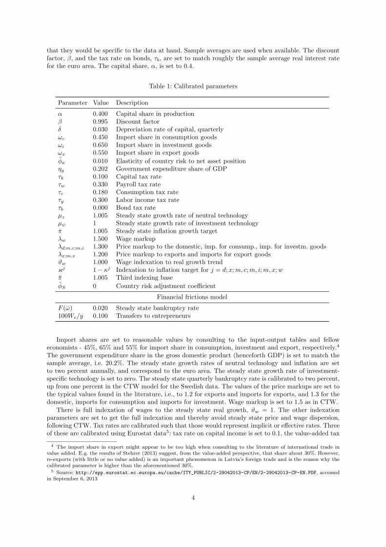
that they would be specific to the data at hand. Sample averages are used when available. The discountfactor, β, and the tax rate on bonds, τb, are set to match roughly the sample average real interest ratefor the euro area. The capital share, α, is set to 0.4.

Table 1: Calibrated parameters

Parameter Value Description

α 0.400 Capital share in productionβ 0.995 Discount factorδ 0.030 Depreciation rate of capital, quarterlyωc 0.450 Import share in consumption goodsωi 0.650 Import share in investment goodsωx 0.550 Import share in export goods

φ̃a 0.010 Elasticity of country risk to net asset positionηg 0.202 Government expenditure share of GDPτk 0.100 Capital tax rateτw 0.330 Payroll tax rateτc 0.180 Consumption tax rateτy 0.300 Labor income tax rateτb 0.000 Bond tax rateµz 1.005 Steady state growth rate of neutral technologyµψ 1 Steady state growth rate of investment technologyπ̄ 1.005 Steady state inflation growth targetλw 1.500 Wage markupλd;m,c;m,i 1.300 Price markup to the domestic, imp. for consump., imp. for investm. goodsλx;m,x 1.200 Price markup to exports and imports for export goodsϑw 1.000 Wage indexation to real growth trendκj 1 − κj Indexation to inflation target for j = d;x;m, c;m, i;m,x;wπ̆ 1.005 Third indexing base

φ̃S 0 Country risk adjustment coefficient

Financial frictions model

F (ω̄) 0.020 Steady state bankruptcy rate100We/y 0.100 Transfers to entrepreneurs

Import shares are set to reasonable values by consulting to the input-output tables and felloweconomists - 45%, 65% and 55% for import share in consumption, investment and export, respectively.4

The government expenditure share in the gross domestic product (henceforth GDP) is set to match thesample average, i.e. 20.2%. The steady state growth rates of neutral technology and inflation are setto two percent annually, and correspond to the euro area. The steady state growth rate of investment-specific technology is set to zero. The steady state quarterly bankruptcy rate is calibrated to two percent,up from one percent in the CTW model for the Swedish data. The values of the price markups are set tothe typical values found in the literature, i.e., to 1.2 for exports and imports for exports, and 1.3 for thedomestic, imports for consumption and imports for investment. Wage markup is set to 1.5 as in CTW.

There is full indexation of wages to the steady state real growth, ϑw = 1. The other indexationparameters are set to get the full indexation and thereby avoid steady state price and wage dispersion,following CTW. Tax rates are calibrated such that those would represent implicit or effective rates. Threeof these are calibrated using Eurostat data5: tax rate on capital income is set to 0.1, the value-added tax

4 The import share in export might appear to be too high when consulting to the literature of international trade invalue added. E.g. the results of Stehrer (2013) suggest, from the value-added perspective, that share about 30%. However,re-exports (with little or no value added) is an important phenomenon in Latvia’s foreign trade and is the reason why thecalibrated parameter is higher than the aforementioned 30%.

5 Source: http://epp.eurostat.ec.europa.eu/cache/ITY_PUBLIC/2-29042013-CP/EN/2-29042013-CP-EN.PDF, accessedin September 6, 2013

4

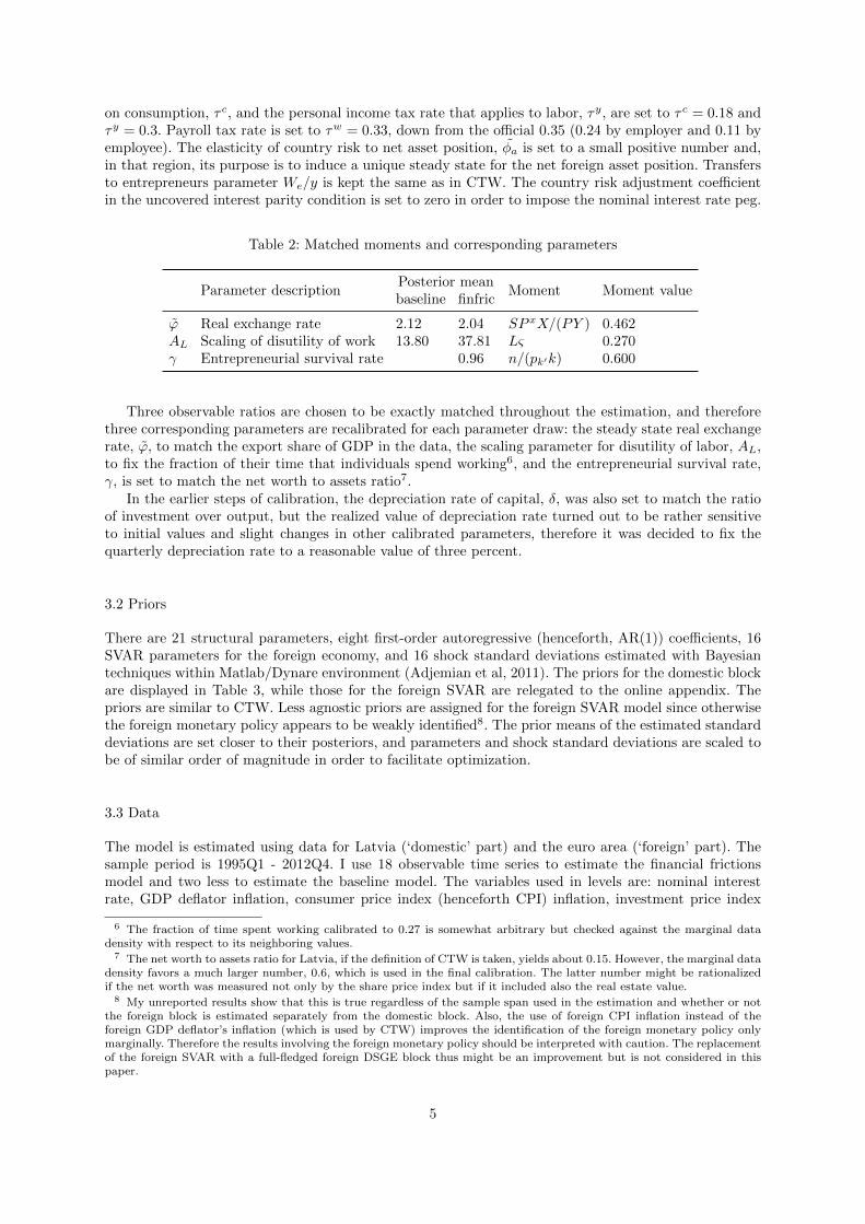
on consumption, τ c, and the personal income tax rate that applies to labor, τy, are set to τ c = 0.18 andτy = 0.3. Payroll tax rate is set to τw = 0.33, down from the official 0.35 (0.24 by employer and 0.11 byemployee). The elasticity of country risk to net asset position, φ̃a is set to a small positive number and,in that region, its purpose is to induce a unique steady state for the net foreign asset position. Transfersto entrepreneurs parameter We/y is kept the same as in CTW. The country risk adjustment coefficientin the uncovered interest parity condition is set to zero in order to impose the nominal interest rate peg.

Table 2: Matched moments and corresponding parameters

Parameter descriptionPosterior mean

Moment Moment valuebaseline finfric

ϕ̃ Real exchange rate 2.12 2.04 SP xX/(PY ) 0.462AL Scaling of disutility of work 13.80 37.81 Lς 0.270γ Entrepreneurial survival rate 0.96 n/(pk′k) 0.600

Three observable ratios are chosen to be exactly matched throughout the estimation, and thereforethree corresponding parameters are recalibrated for each parameter draw: the steady state real exchangerate, ϕ̃, to match the export share of GDP in the data, the scaling parameter for disutility of labor, AL,to fix the fraction of their time that individuals spend working6, and the entrepreneurial survival rate,γ, is set to match the net worth to assets ratio7.

In the earlier steps of calibration, the depreciation rate of capital, δ, was also set to match the ratioof investment over output, but the realized value of depreciation rate turned out to be rather sensitiveto initial values and slight changes in other calibrated parameters, therefore it was decided to fix thequarterly depreciation rate to a reasonable value of three percent.

3.2 Priors

There are 21 structural parameters, eight first-order autoregressive (henceforth, AR(1)) coefficients, 16SVAR parameters for the foreign economy, and 16 shock standard deviations estimated with Bayesiantechniques within Matlab/Dynare environment (Adjemian et al, 2011). The priors for the domestic blockare displayed in Table 3, while those for the foreign SVAR are relegated to the online appendix. Thepriors are similar to CTW. Less agnostic priors are assigned for the foreign SVAR model since otherwisethe foreign monetary policy appears to be weakly identified8. The prior means of the estimated standarddeviations are set closer to their posteriors, and parameters and shock standard deviations are scaled tobe of similar order of magnitude in order to facilitate optimization.

3.3 Data

The model is estimated using data for Latvia (‘domestic’ part) and the euro area (‘foreign’ part). Thesample period is 1995Q1 - 2012Q4. I use 18 observable time series to estimate the financial frictionsmodel and two less to estimate the baseline model. The variables used in levels are: nominal interestrate, GDP deflator inflation, consumer price index (henceforth CPI) inflation, investment price index

6 The fraction of time spent working calibrated to 0.27 is somewhat arbitrary but checked against the marginal datadensity with respect to its neighboring values.

7 The net worth to assets ratio for Latvia, if the definition of CTW is taken, yields about 0.15. However, the marginal datadensity favors a much larger number, 0.6, which is used in the final calibration. The latter number might be rationalizedif the net worth was measured not only by the share price index but if it included also the real estate value.

8 My unreported results show that this is true regardless of the sample span used in the estimation and whether or notthe foreign block is estimated separately from the domestic block. Also, the use of foreign CPI inflation instead of theforeign GDP deflator’s inflation (which is used by CTW) improves the identification of the foreign monetary policy onlymarginally. Therefore the results involving the foreign monetary policy should be interpreted with caution. The replacementof the foreign SVAR with a full-fledged foreign DSGE block thus might be an improvement but is not considered in thispaper.

5

inflation, foreign CPI inflation, foreign nominal interest rate and the interest rate spread. The rest ofthe variables are in terms of the first differences of logs, and these are: real GDP, real consumption, realinvestment, real exports, real imports, real government expenditures, real wage, real exchange rate, realstock price index, total hours worked, and real foreign GDP. All the differenced variables are demeanedexcept for total hours worked. The domestic inflation rates and the real exchange rate are demeaned aswell. All real quantities are in per capita terms. All foreign variables correspond to the euro area data.

3.4 Shocks and measurement errors

In total, there are 18 exogenous stochastic variables in the theoretic financial frictions model: four tech-nology shocks - stationary neutral technology, ε, stationary marginal efficiency of investment, Υ , unit-rootneutral technology, µz, and unit-root investment specific technology, µΨ , - a shock to consumption pref-erences, ζc, and to disutility of labor supply, ζh, a shock to government expenditure, g, and a countryrisk premium shock that affects the relative riskiness of foreign assets compared to domestic assets, φ̃.There are five markup shocks, one for each type of intermediate good, τd, τx, τm,c, τm,i, τm,x (d -domestic, x - exports, m, c - imports for consumption, m, i - imports for investment, m,x - imports forexports). The financial frictions model has two more shocks - one to idiosyncratic uncertainty, σ, andone to entrepreneurial wealth, γ. There are also shocks to each of the foreign observed variables - foreignGDP, y∗, foreign inflation, π∗, and foreign nominal interest rate, R∗.

The stochastic structure of the exogenous variables are the following: eight of these evolve accordingto AR(1) processes:

εt, Υt, ζct , ζ

ht , gt, φ̃t, σt, γt

Five shock processes are i.i.d.:

τdt , τxt , τ

m,ct , τm,it , τm,xt

and five shock processes are assumed to follow a first-order SVAR:

y∗t , π∗t , R

∗t , µz,t, µΨ,t.

As in CTW, two shocks are suspended in the estimation: the shock to unit-root investment specifictechnology, µΨ,t, and the idiosyncratic entrepreneur risk shock, σt. The first one should correspond tothe foreign block but its identification is dubious in the particular SVAR model; the second has beenfound to have limited importance in CTW9.

There are measurement errors except for domestic interest rate and the foreign variables. The varianceof the measurement errors is calibrated to correspond to 10% of the variance of each data series.

4 Results

The domestic and foreign blocks are estimated separately since Latvia’s economy has a minuscule effect onthe euro area. The estimation results for the foreign SVAR model are obtained using a single Metropolis-Hastings chain with 100 000 draws after a burn-in of 900 000 draws. For the domestic block, the estimationresults are obtained using two Metropolis-Hastings chains, each with 50 000 draws after a burn-in of 200000 draws. Prior-posterior plots are relegated to the online appendix.

4.1 Posterior parameter values

The posterior parameter estimates for the domestic block are reported in Table 3, while those specific tothe foreign SVAR are relegated to the online appendix. The priors were deliberately fixed to be the sameacross the two models for a more transparent comparison, and favor the baseline model. The estimatedmode of the elasticity of substitution of investment goods parameter, ηi, is close to unity and thus the

9 Christiano, Motto and Rostagno (2014) find (the anticipated part of) this shock important when loans are observable.My unpublished results show that fitting loans may require excessive amount of risk.

6

parameter is calibrated for the financial frictions model to 1.1, similar to the posterior mean in thebaseline model, in order to avoid numerical issues.

The most notable difference between the estimated parameters across the models is in the investmentadjustment costs parameter which is about 2.5 times lower for the financial frictions model comparedto the baseline specification. They are statistically significantly different at a 5% significance level. Thelower parameter indicates that the financial frictions model induces the gradual response that the in-vestment adjustment mechanism was introduced to generate. Also, the estimated persistence parameterof the marginal efficiency of investment (henceforth MEI) shock is reduced (from 0.80 to 0.59) with theintroduction of the financial frictions block. Regarding the estimated standard deviations of shocks, thefinancial frictions model assigns a smaller standard deviation to the marginal efficiency of investmentshock, which, apparently, is ‘crowded out’ by the entrepreneurial wealth shock.

Comparing the overall fit of the models in terms of the marginal data density (based on a commonset of observables and estimated parameters for both models), the posterior odds ratio is 1:3.5 × 1014 infavor of the financial frictions model (see Table 3).

4.2 Model moments and variance decomposition

4.2.1 Model moments

Table 4 presents the data and the model means and standard deviations for the observed time series.The table shows that there is a substantial variation of growth rates in the data, especially betweenthe domestic and foreign variables, which is why real quantities, the domestic inflation rates and thereal exchange rate are demeaned before matching the model to the data. The standard deviations arematched rather well but their over-estimation is evident for total hours, GDP, imports, as well as forthe interest rate spread10. The introduction of the financial frictions block appears to slightly lessen thisover-estimation issue.

Table 4: Data and (first-order approximated) model moments (in percent)

Variable ExplanationMean Standard deviation

DataModel

DataModel

baseline finfric baseline finfric

π Domestic inflation 6.08 2.00 2.00 8.39 8.77 8.60πc CPI inflation 5.62 2.00 2.00 6.29 8.78 8.71πi Investment inflation 6.78 2.00 2.00 51.45 50.70 45.72R Nom. interest rate 7.06 6.04 6.04 5.86 5.75 6.37∆h Total hours growth 0.02 0.00 0.00 2.20 6.92 5.60∆y GDP growth 1.37 0.50 0.50 2.31 5.49 4.49∆w Real wage growth 1.06 0.50 0.50 2.35 2.95 2.91∆c Consumption growth 1.47 0.50 0.50 2.84 3.19 3.42∆i Investment growth 1.73 0.50 0.50 16.32 21.28 22.20∆q Real exch. rate growth -0.88 0.00 0.00 2.51 2.28 2.27∆g Gov. expendit. growth 0.44 0.50 0.50 5.46 5.26 5.31∆x Export growth 2.19 0.50 0.50 3.41 3.70 3.61∆m Import growth 2.22 0.50 0.50 6.30 12.46 9.67∆n Stock market growth 1.32 0.50 10.38 14.78spread Interest rate spread 4.29 3.02 2.25 5.52∆y∗ Foreign GDP growth 0.26 0.50 0.50 0.61 0.52 0.52π∗ Foreign inflation 2.01 2.00 2.00 0.72 0.88 0.88R∗ Foreign nom. int. rate 3.16 6.04 6.04 1.61 2.58 2.58

Note: 1) The model moments are theoretical, i.e. computed based on calibrated parameters or their posterior means. Assuch, the model moments are not subject to sampling uncertainty, as in the case of simulated moments.2) The inflation and interest rates are annualized.

10 CTW note that their use of ‘endogenous prior’ reduces the effect of over-estimated shock standard deviations. I’m notusing such a prior.

7

4.2.2 Conditional variance decomposition

The conditional variance decomposition at eight quarters forecast horizon is reported in Table 5.

Table 5: Conditional variance decomposition (percent) given model parameter uncertainty at 8 quartersforecast horizon; posterior mean

Description model R πc GDP C I NXGDP

H w q N Spread

εtStationarytechnology

B 0.0 2.3 1.3 0.3 0.1 0.3 9.1 1.4 2.1F 0.0 0.6 0.7 0.1 0.0 0.5 8.6 0.3 0.6 0.1 0.1

Υt MEIB 5.2 0.9 14.5 0.4 78.3 66.8 5.9 1.0 0.9F 0.1 0.0 1.8 0.1 19.2 3.4 3.2 0.2 0.0 12.7 12.2

ζct Consumption prefsB 0.1 0.1 1.7 77.9 0.3 1.8 1.3 0.0 0.1F 0.2 0.0 7.1 78.7 0.1 14.8 5.6 0.0 0.0 0.1 0.1

ζht Labor prefsB 0.1 14.1 5.6 3.5 1.1 0.8 5.5 41.4 12.7F 0.1 10.1 5.8 4.0 1.0 6.6 8.0 51.7 9.3 2.0 0.6

τdt Markup, domesticB 0.0 34.6 2.1 0.1 0.1 0.3 1.4 43.4 31.3F 0.0 22.7 2.2 0.1 0.1 0.3 1.8 33.0 20.8 0.5 0.1

τxt Markup, exportsB 0.0 0.0 1.3 0.0 0.0 0.0 1.0 0.0 0.0F 0.0 0.0 2.3 0.0 0.0 0.0 1.8 0.0 0.0 0.0 0.0

τmctMarkup, imp. forcons.

B 0.0 36.8 1.6 0.0 0.0 0.3 1.3 2.3 33.2F 0.0 59.1 4.1 0.1 0.0 1.1 3.2 3.9 54.1 0.1 0.0

τmitMarkup, imp. forinv.

B 0.9 3.8 29.8 0.1 5.8 11.9 42.5 1.5 3.4F 0.1 0.3 23.3 0.0 5.4 6.0 34.4 0.1 0.3 7.9 6.1

τmxtMarkup, imp. forexp.

B 0.3 0.1 35.6 0.1 0.1 6.2 27.8 0.1 0.1F 0.1 0.0 28.4 0.1 0.1 6.2 22.8 0.1 0.0 0.2 0.1

γtEntrepreneurialwealth

BF 0.7 0.6 10.1 0.2 58.1 38.9 1.1 0.6 0.5 62.4 77.3

φ̃tCountry riskpremium

B 86.0 0.2 0.6 1.2 3.1 7.1 0.3 0.6 0.1F 91.8 0.4 2.2 5.5 8.7 17.8 0.8 3.1 0.4 9.4 1.7

µz,tUnit-roottechnology

B 1.7 0.1 0.2 0.2 0.1 1.4 0.0 0.4 0.3F 1.7 0.0 0.2 0.0 0.1 1.4 0.0 0.2 0.2 0.1 0.0

εR∗,tForeign interestrate

B 1.8 0.1 0.0 0.1 0.3 0.8 0.0 0.0 0.0F 1.6 0.1 0.1 0.3 0.3 0.7 0.0 0.1 0.0 0.2 0.0

εy∗,t Foreign outputB 3.7 0.2 0.0 0.3 0.5 2.3 0.0 0.1 0.2F 3.6 0.1 0.0 0.8 0.2 2.1 0.0 0.3 0.2 0.0 0.0

επ∗,t Foreign inflationB 0.1 0.0 0.0 0.0 0.0 0.0 0.0 0.0 0.1F 0.1 0.0 0.0 0.0 0.0 0.0 0.0 0.0 0.1 0.0 0.0

5 foreign*B 93.3 0.5 0.8 1.7 4.0 11.6 0.4 1.2 0.7F 98.7 0.6 2.6 6.6 9.3 22.0 0.8 3.6 0.9 9.7 1.8

All foreign**B 94.5 41.2 69.1 1.9 9.9 30.0 73.0 5.1 37.5F 98.9 60.1 60.7 6.8 14.9 35.3 63.1 7.8 55.3 17.9 8.0

Note: R - nominal interest rate, πc - CPI inflation, C - real consumption, I - real investment, NX/GDP - net exports toGDP ratio, H - total hours, w - real wage, q - real exchange rate, N - real net worth.∗ ‘5 foreign’ is the sum of the foreign stationary shocks, R∗t , π∗t , Y ∗t , the country risk premium shock, φ̃t, and the world-wideunit root neutral technology shock, µz,t.∗∗ ‘All foreign’ includes the above five shocks as well as the markup shocks to imports and exports, i.e. τmct , τmit , τmxtand τxt . ‘B’ - baseline model, ‘F’ - financial frictions model.

Entrepreneurial wealth shock versus marginal efficiency of investment shock Table 5 shows that theentrepreneurial wealth shock, which is specific to the financial frictions model and absent from thebaseline model, ‘crowds out’ the marginal efficiency of investment (MEI) shock by reducing its share ofexplaining the variance of investment from 78% (baseline) to 19% (financial frictions model), the varianceof net exports to GDP ratio from 67% to 3%, and the variance of GDP from 15% to 2%.11

The entrepreneurial wealth shock explains 10% of the variance of GDP, 58% of the variance ofinvestment, 39% of the net exports to GDP ratio, 62% of entrepreneurial net worth and 77% of thespread between the nominal interest rate paid by the entrepreneur and the risk-free one.

11 As a reminder, MEI shock enters in the capital accumulation equation and affects how (efficiently) investment istransformed into capital. This is the shock whose importance is emphasized in Justiniano, Primiceri and Tambalotti(2011), where one of their interpretations of this shock being a proxy for the effectiveness with which the financial sectorchannels the flow of the household savings into a new productive capital.

8

CTW do not report the conditional variance decomposition for the baseline model, but with thefinancial frictions together with the search and matching frictions in labor market (without additionalshock added) which are absent in my financial frictions model. Also, their model is estimated for Swedishdata with inflation-targeting monetary policy. Nevertheless, it is instructive to compare the results ofCTW with mine. The results of CTW suggest that, when financial frictions mechanism is present, MEIshock explains 10% of the variance of investment, 7% of the variance of net exports to GDP ratio, and 4%of the variance of GDP. Also, the entrepreneurial wealth shock explains 71% of the variance of investment,23% of the variance of the net exports to GDP ratio, 25% of the variance of GDP, 64% of entrepreneurs’net worth, and 60% of the variance of the spread. CTW briefly mention, but do not report in tables,the effect of shutting down the financial shock in their model. In that case, MEI shock becomes moreimportant in the variance decomposition: it explains 52% of the variance of investment and 6% of GDP.These results are broadly in line with mine except for the variance of investment which appears to bebetter explained by the entrepreneurial wealth shock than by MEI shock in Sweden compared to Latvia.The difference is likely due to the milder response of entrepreneurial net worth to the wealth shock inLatvia compared to Sweden, reflecting the fact that Swedish financial markets are more developed.

Country risk premium shock Table 5 also reports that the country risk premium shock is the majordriving force of the domestic nominal interest rate and an important factor for Latvia’s investment.This is more so in the financial frictions model compared to the baseline. So, for the given sample of1995Q1-2012Q4, the country risk premium shock explains 92% of the variance of the domestic nominalinterest rate (versus 86% in baseline), 9% of the variance of investment (versus 3% in baseline), 2% ofthe variance of GDP (versus 1% in baseline), 18% of the variance of net exports to GDP ratio (versus7% in baseline) and 9% of the variance of the entrepreneurs’ net worth.

Comparing to the results of CTW, there are big differences. For Sweden, this shock explains only 5%of the variance of nominal interest rate, 1% of the variance of investment, and 1% of the variance of networth, while the variance of GDP is explained by about the same amount as in Latvia. The reason forthe difference is that, during the specific historic sample, the domestic nominal interest rate in Latvia hasbeen higher than in the euro area and given that, in the model, Latvia’s currency is hard-pegged to theeuro, the (huge historic) difference between the actual domestic and foreign interest rates is explainedby the country risk premium. It is expected that, since Latvia’s joining the euro area in 2014, the weightof the country risk premium shock on the domestic interest rate will diminish, giving more influence tothe euro area-wide shocks.

Shocks in the foreign economy block The effect of the foreign interest rate, foreign output and foreigninflation shocks on the domestic economy is estimated to be rather limited, with the greatest influencebeing to the domestic nominal interest rate. The unit-root technology shock also has been estimated tohave little influence on the domestic economy during the particular historic period.

These results are broadly close to the results of CTW who also find negligible role of the shock toforeign interest rate, foreign output and foreign inflation to Swedish economy. Though, their estimatedeffect of the unit-root technology shock is more influential, explaining 4.1% of the variance of SwedishGDP compared to 0.2% for Latvia’s GDP. The latter result might be explained by the fact that, duringthe particular historic episode, Latvia’s economy has been on its more or less idiosyncratic catching-upboom-bust cycle, while the more developed Swedish economy has been more reliant on the world-widetechnology growth. Also, CTW estimate this shock based on the trade-weighted foreign variables, whileI use the euro area variables, thus the link (the common technology) between the domestic and foreignvariables is looser in my case.

Stationary neutral technology shock While touching upon technology shocks, another difference betweenCTW results for Sweden and mine for Latvia is in the effect of the stationary neutral technology shockaffecting the intermediate goods producers’ production function. This shock is estimated to have minorinfluence on Latvia’s economy except for total hours worked (9% of the variance explained by this shock).

CTW estimation shows that this shock explains about the same portion of the variance of hoursworked but also 11% of the variance of consumption (0.1% for Latvia), 9% of the variance of GDP (0.7%for Latvia), 6% of CPI inflation (0.6% for Latvia) and 8% of the domestic nominal interest rate (0.0%for Latvia). Apparently, other domestic shocks have compensated the lack of influence of the stationarytechnology shock on Latvia’s economy.

9

Household preference shocks Noticeable, the consumption preference shock explains 79% of the variationof consumption in Latvia, whereas ‘only’ 45% in Sweden. This difference might be explained by thestrong consumption-driven boom that Latvia experienced starting around 2004 (see the historic shockdecomposition below).

The labor preference shock is estimated to have similar effect on both countries with respect towages; this shock is estimated to explain 52% and 39% of the variance of real wages in Latvia andSweden, respectively. The effect on total hours worked differ, but this is probably due to the differentstructure of labor market modeling block in the models.

Domestic markup shock The domestic markup shock, affecting marginal cost of producing the domesticintermediate good, is estimated to explain 23% of Latvia’s CPI inflation (45% in Sweden) and 33% of thevariance in real wage (31% in Sweden). This completes the similarities of this shock across the countries,since, given Latvia’s peg regime, this shock explains 21% of the variance of Latvia’s real exchange rate(0.2% in Sweden), while in Sweden, it affects, through Taylor rule, the nominal interest rate, and partsof real economy stronger than in Latvia; e.g. it explains 7% of the variance of Swedish GDP and 3% ofthe variance of Swedish investment, while these figures are 2% and 0.1% for Latvia.

Export goods markup shock Table 5 shows that the markup shock to export goods is estimated to havelittle effects on Latvia’s economy; the only noticeable ones are the 2% (up from 1% in baseline) of thevariance of GDP and hours worked, while in Sweden these figures are 8% and 10%, respectively. Again,given the model differences, it is hard to point exact source of the discrepancy. A small part of thedifference12 is due to the higher calibrated imported goods share in exports for Latvia (55%) than forSweden (35%), resulting in a smaller effect of the exports markup on Latvia’s GDP and hence hoursworked, since the markup to imports for exports is subject to a separate shock.

Imports markup shocks The imports for exports markup shock, indeed, has more weight on Latvia’seconomy than on Swedish: it is estimated to explain 28% of the variance of Latvia’s GDP (16% forSweden) and 23% of the variance of total hours worked in Latvia (14% in Sweden).13

Regarding the rest of the imports goods markup shocks, the imports for consumption markup shockexplains the majority, 59% of the variance of the the domestic CPI inflation (up from 37% in baselineand 34% in Sweden), and hence is the major shock affecting the real exchange rate - it explains 54% (upfrom 33% in baseline) of the variance of Latvia’s real exchange rate, while in Sweden, this shock explains,through Taylor rule, 17% of the variance of the nominal interest rate but less so the real exchange rate. Incontrast to the domestic markup shock, the imports for consumption markup shock is estimated to havea non-negligible effect on Latvia’s GDP - it explains 4% of the variance of Latvia’s GDP, while only 0.2%of Swedish GDP. The importance of this effect, again, can be explained by the strong consumption-drivenboom Latvia’s economy experienced during the considered sample span.

Finally, the imports for investment markup shock explains 5% of the variance of investment, 23% ofthe variance of GDP, and 34% (down from 43% in baseline) of the variance of total hours worked. Quitedifferently, this shock is estimated to have negligible effect on Swedish economy. The explanations for thedifference might be i) the higher calibrated import share in investment goods for Latvia (65%) than inSweden (43%), ii) the differences in the structure of the labor market block, and iii) the noise in Latvianinvestment inflation data.

Foreign shocks combined Overall, if the foreign shocks are defined as the three foreign (interest rate,output, inflation) stationary shocks, the country risk premium shock, the world-wide unit root neutraltechnology shock, the markup shocks to imports (imports for exports, consumption, investment) andexports - in total, nine shocks - see the bottom row of Table 5, then they explain 99% of the variance inthe domestic nominal interest rate (up from 28% in Sweden), the overwhelming part explained by thecountry risk premium shock. Also, 60% and 61% of the variations of CPI inflation and GDP, respectively,(versus 40% and 32% in Sweden) at two year forecast horizon are explained by the foreign shocks, the

12 I have checked this claim by recalibrating the model.13 My unpublished results show that when data measurement errors are estimated, the imports for exports markup shock

is almost eliminated. The true source of this shock is yet to be determined.

10

overwhelming portion coming from markup shocks to imports for consumption and domestic goods (forCPI inflation) and to imports for exports and imports for investment (for GDP).

Since, in the literature, the sources of business cycles are largely related to fluctuations in investment,the major source of the variance of investment in Latvia is estimated to be the entrepreneurial wealthshock. Given the evidence from Sweden, the influence of this shock is to be expected to grow as Latvia’sfirms become more financially integrated.

4.3 Impulse response functions

Since Table 5 shows that the entrepreneurial wealth shock is the main driver of the variance of investmentin the financial frictions model and that it ‘crowds out’ MEI shock from the baseline model, it is instructiveto compare the impulse response functions (henceforth IRF) of these two shocks.

Entrepreneurial wealth shock The IRF to the entrepreneurial wealth shock are plotted in Figure 1, whichshows that a positive temporary entrepreneurial wealth shock, γt, drives up the net worth, reduces theexpected bankruptcy rate and thus the interest rate spread, and increases the investment (by about thesame percentage change as in net worth); GDP goes up accordingly, and so do the real wage and totalhours worked. Both exports and imports increase but the latter increases more due to the demand forinvestment goods, thus net exports to GDP ratio decreases slightly. As a consequence, the net foreignassets to GDP ratio worsens, driving up a slight risk premium on the domestic nominal interest rate. Theshock causes the cost of investment to decrease, and consumption to pick up only steadily. Therefore,CPI inflation decreases, though by a small amount, and thus the real exchange rate depreciates.

The response of net worth to this and other shocks is quite muted, i.e. its dynamics appear to dieout in a few periods. This observation together with the autocorrelated measurement error of net worthsuggest that the stock market price index might be a weak proxy for net worth in Latvia, and thus otherpotential measures, such as the house price index, could be investigated. Such an option is left for futureresearch.

Entrepreneurial wealth shock

finfric 95% finfric mean baseline foreign5 10 15 20

−0.3−0.2−0.1

Net foreign assets/GDP (Lev.dev.)

5 10 15 20−2

−1

Spread (APP)

5 10 15 2005

10

Net worth (% dev.)5 10 15 20

00.05

0.1

Real exch. rate (% dev.)

5 10 15 200

0.050.1

Real wage (% dev.)

5 10 15 20−0.2

00.20.40.60.8

Total hours (% dev.)5 10 15 20

−0.03−0.02−0.01

00.01

Net exports/Y (Lev. dev.)

5 10 15 20

05

10

Investment (% dev.)

5 10 15 20

−0.10

0.1

Consumption (% dev.)5 10 15 20

0

0.5

1GDP (% dev.)

5 10 15 20

−0.4−0.2

0

CPI inflation (APP)

5 10 15 200

0.20.40.6

Nom. interest rate (APP)

Fig. 1: Impulse responses to the entrepreneurial wealth shock, γt.

Note: The units on the y-axis are either in terms of percentage deviation (% dev.) from the steady state, annual percentagepoints (APP), or level deviation (Lev. dev.).

11

MEI shock Comparing the wealth shock to a temporary MEI shock, Figure 2 shows that the effect ofMEI shock in the baseline model is qualitatively similar to the effect of the wealth shock in the financialfrictions model (except for the effect on consumption which decreases initially), but the introductionof financial frictions dampens the effect of MEI shock on all plotted variables (and consumption nowslightly increases). The changes in IRF are statistically significant at a 5% significance level. The effectof these shocks on net worth and the spread is opposite; this is how the two shocks are distinguished inthe financial frictions model.

MEI shock increases the amount of capital per investment and thus the price of capital decreases.Consumption barely moves, thus MEI shock has a downward pressure on prices.

Marginal efficiency of investment shock


−0.3−0.2−0.1

0


5 10 15 200

0.5

1Spread (APP)

5 10 15 20

−6−4−2

0

Net worth (% dev.)5 10 15 20

−0.020

0.020.040.060.08


5 10 15 200

0.050.1

Real wage (% dev.)

5 10 15 20

00.5

11.5


−0.04−0.02

00.02

Net exports/Y (Lev. dev.)

5 10 15 20

05

10

Investment (% dev.)

5 10 15 20

−0.10

0.1


00.5

1

GDP (% dev.)

5 10 15 20

−0.3−0.2−0.1

0

CPI inflation (APP)

5 10 15 200

0.20.40.6


Fig. 2: Impulse responses to the marginal efficiency of investment shock, Υt.


Country risk premium shock Figure 3 shows the IRF to a temporary country risk premium shock. AsTable 5 shows, this shock is the major cause of the variance of the domestic nominal interest rate.The effects are qualitatively similar across the models but the financial frictions mechanism somewhatamplifies them. The shock increases the domestic nominal interest rate which decays towards its steadystate with persistence. This is followed by a decrease in consumption and entrepreneurial net worth, anincrease in the spread and the bankruptcy rate (both reverse the sign after a year), and a decrease ininvestment (initially, about twice as much with financial frictions mechanism compared to the baseline),GDP, real wage, and total hours worked. Imports decrease more than exports, resulting in a negligibleincrease in net exports to GDP ratio. CPI inflation decreases for about two years. The real exchangerate thus depreciates for the first two years after the shock.

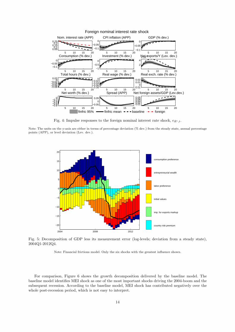
Foreign nominal interest rate shock Table 5 shows that the foreign nominal interest rate shock has littleinfluence on the domestic economy during the particular historic period; nevertheless, policy-makers areusually interested in what happens when the policy rate changes, and it is the European Central Bank’spolicy rate that matters for Latvia after it joined the euro area in 2014. Figure 4 shows that a positivetemporary foreign nominal interest shock increases both the foreign and the domestic nominal interestrate by the same amount, and both decay towards their steady state slowly. Consumption, investmentand entrepreneurial net worth decrease, bankruptcy rate increases (for the first year) and, as a result, sodoes the spread. GDP decreases, so do real wage and total hours worked. There is a negligible increasein net exports to GDP ratio due to a decrease in imports. Thus, the net foreign assets to GDP ratio

12

Country risk premium shock


0.050.1

0.150.2

0.25


5 10 15 20−0.4−0.2

00.20.4

Spread (APP)

5 10 15 20−6−4−2

0

Net worth (% dev.)5 10 15 20

−0.050

0.050.1


5 10 15 20−0.4−0.2

0

Real wage (% dev.)

5 10 15 20

−0.4−0.2

0


01020

x 10−3Net exports/Y (Lev. dev.)

5 10 15 20−6−4−2

0

Investment (% dev.)

5 10 15 20−0.6−0.4−0.2

0


−0.6−0.4−0.2

0

GDP (% dev.)

5 10 15 20−0.4−0.2

00.2

CPI inflation (APP)

5 10 15 2001

2


Fig. 3: Impulse responses to the country risk premium shock, φ̃t.


increases slightly, fostering a decrease of the domestic country risk premium, and therefore, also of thedomestic nominal interest rate. CPI inflation decreases due to the slower domestic activity. The domesticinflation decreases by a larger amount than the foreign inflation, resulting in the initial depreciation ofthe real exchange rate. The effect is similar across the models except for the more persistent dynamicsof the nominal interest rate under the financial frictions mechanism.

The impulse response functions are similar between the country risk premium and the foreign nominalinterest rate shocks, thus signaling the potential identification issues of these two shocks. The particularprocedure of estimating the foreign SVAR separately from the domestic block mitigates the identificationproblem somewhat. The replacement of the foreign SVAR with a full-blown foreign DSGE block couldbe a cure since it would identify the foreign monetary policy better but at the cost of model complexity.

The rest of the IRF are plotted in the online appendix.

4.4 Historical shock decomposition

Figures 5 to 10 show the historic shock decomposition of GDP, CPI inflation and the interest rate spread.

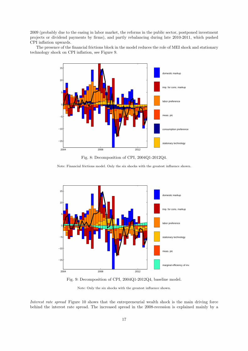
GDP Concentrating on the most sizable shocks, Figure 5 shows that the model identifies the shock tohousehold consumption preferences as the most important driving force of the 2004-boom. During theperiod of 2004-2007, the values of this shock were persistently above the sample average (see smoothedshock figures in the online appendix), signifying that households were especially keen on spending onconsumption goods during that period. The shock ceased during the second half of 2007, probably dueto the rising costs of living and thus the decreasing consumer confidence (the latter claim is backed bythe ECFIN consumer survey data). At that time several other shocks became adverse, including thestationary and unit-root neutral technology shocks, and the risk premium shock. Starting from 2008 andup to 2011, a series of negative entrepreneurial wealth shocks is identified to have significantly affectedGDP growth. In fact, this shock has become the major source determining the GDP level during the post-recession episode. In the model, the dynamics of the entrepreneurial wealth is observable and measuredby the NASDAQ OMX Riga share price index, which plummeted during the recession. In practice, it islikely that the variable captures also a part of the dynamics in the real estate prices (otherwise, the realestate sector is not present in the model), which also fell sharply during the recession as a result of theburst of the housing bubble.

13

Foreign nominal interest rate shock


0.010.020.030.040.05


5 10 15 20−0.05

00.05

Spread (APP)

5 10 15 20−0.8−0.6−0.4−0.2

0

Net worth (% dev.)5 10 15 20

−0.010

0.010.02


5 10 15 20−0.08−0.06−0.04−0.02

0

Real wage (% dev.)

5 10 15 20−0.08−0.06−0.04−0.02

00.02


2

4x 10

−3Net exports/Y (Lev. dev.)

5 10 15 20−1

−0.5

0

Investment (% dev.)

5 10 15 20

−0.1−0.05

0


−0.1

−0.05

0

GDP (% dev.)

5 10 15 20

−0.1

−0.05

0CPI inflation (APP)

5 10 15 200.05

0.10.15

0.20.25


Fig. 4: Impulse responses to the foreign nominal interest rate shock, εR∗,t.


2004 2008 2012

−20

−15

−10

−5

0

5

10

15

20

country risk premium

imp. for exports markup

initial values

labor preference

entrepreneurial wealth

consumption preference

Fig. 5: Decomposition of GDP less its measurement error (log-levels; deviation from a steady state),2004Q1-2012Q4.

Note: Financial frictions model. Only the six shocks with the greatest influence shown.

For comparison, Figure 6 shows the growth decomposition delivered by the baseline model. Thebaseline model identifies MEI shock as one of the most important shocks driving the 2004-boom and thesubsequent recession. According to the baseline model, MEI shock has contributed negatively over thewhole post-recession period, which is not easy to interpret.

14

2004 2008 2012

−15

−10

−5

0

5

10

15

20

25

imp. for exports markup

imp. for inv. markup

foreign interest rate


labor preference

marginal efficiency of inv.

Fig. 6: Decomposition of GDP less its measurement error (log-levels; deviation from a steady state),2004Q1-2012Q4, baseline model.

Note: Only the six shocks with the greatest influence shown.

Therefore, having the financial frictions block in the model both clarifies and changes the story.First, the entrepreneurial wealth shock behaves differently than MEI shock, since the former has playedlittle role during the boom period. Thus, consumption preferences are left as the single most importantfactor creating the 2004-boom. Second, the entrepreneurial wealth shock is more easily understandableforce that has deepened the recession but ceased to be active during the post-recession episode. On thecontrary, in the baseline model, the ever-active MEI shock during the post-recession period is harder toexplicate.

The results of the financial frictions model are supported by a model-free decomposition of GDPannual growth into its expenditure components, which shows that the GDP 2004-boom was driven mainlyby private consumption, and the 2008-bust resulted in a sharp decline in both private consumption andgross fixed capital formation (Figure 7).

15

2004 2008 2012

−30

−20

−10

0

10

20

30

private consumption

govt. spending

gross fixed capit. form.

changes in inventories

exports

imports

Fig. 7: Model-free decomposition of GDP (undemeaned annual growth rates) into its expenditure com-ponents, 2004Q1-2012Q4.

Note: Seasonally adjusted series are used, thus the sum of the contributions of components do not exactly match the GDPgrowth rates.

CPI inflation Figure 8 shows that the model identifies the shock to household labor preferences asthe major driving force of Latvia’s CPI inflation up in the 2004-boom, coupled with the imports forconsumption markup shock in 2007-2008, and these same shocks together with the domestic markupshock drew CPI inflation down in 2009.

The labor preference shock reflects the household willingness to work14. The model identifies that,during the period of 2005-2007 households in Latvia were keen to work less (and to consume more),relative to the sample average. The disutility from work arose probably due to the rapidly growingeconomy and thus the relatively easy money available for spending. Tight labor market drove wages upto compensate for the household disutility from work; and that in turn, pushed the price of consumptiongoods up. Beginning in late 2008 and continuing until the sample ends in 2012Q4, the labor preferenceshock is identified to have downward pressure on CPI inflation, which could be explained by the increasednecessity to earn a living due to lower wages and fewer job opportunities.

The markup shock to imports for consumption goods raises the price of imports for consumptiongoods. The model identifies that the level of this shock was persistently above its sample average duringthe year 2008, the time at which the consumption preference shock had already become flat or evennegative, and coinciding with the period of the above average foreign inflation shock (unaffected by thedomestic block, since estimated separately) and the peak in both crude oil and natural gas prices. It islikely that the imports for consumption markup shock captures the increase in the cost of energy, sincethe price of energy is not present in the model but through foreign inflation. Apparently, the foreigninflation variable is not able to fully represent the dynamics of imported costs, thus the rest is absorbedby the markup shock. For example, the price of natural gas affects the heating bills. It was a matterof fact that heating bills rose during the year 2008, constituting up to three percentage points of theannual inflation at that time. Overall, the model suggests that the imports for consumption markupshock constituted about a half of the annual CPI inflation during the year 2008.

The domestic markup shock affects the marginal cost of domestic production before it is affectedby the foreign markup shocks. The model identifies a series of negative domestic markup shock during

14 The labor preference shock reflects the supply side in the labor market, and thus it can be affected by ‘long-run’ factorssuch as demographics and labor force participation rate. Indeed, the latter increased during the boom years in 2006-2007and decreased during the recession in 2009-2010. Therefore, the participation rate has dampened the cyclical fluctuationsof the labor preference shock. See Christiano, Trabandt and Walentin (2010) for a model with endogenous participationrate.

16

2009 (probably due to the easing in labor market, the reforms in the public sector, postponed investmentprojects or dividend payments by firms), and partly rebalancing during late 2010-2011, which pushedCPI inflation upwards.

The presence of the financial frictions block in the model reduces the role of MEI shock and stationarytechnology shock on CPI inflation, see Figure 9.

2004 2008 2012

−15

−10

−5

0

5

10

15

stationary technology


meas. pic

labor preference

imp. for cons. markup

domestic markup

Fig. 8: Decomposition of CPI, 2004Q1-2012Q4.


2004 2008 2012

−15

−10

−5

0

5

10

15


meas. pic

stationary technology

labor preference

imp. for cons. markup

domestic markup

Fig. 9: Decomposition of CPI, 2004Q1-2012Q4, baseline model.

Note: Only the six shocks with the greatest influence shown.

Interest rate spread Figure 10 shows that the entrepreneurial wealth shock is the main driving forcebehind the interest rate spread. The increased spread in the 2008-recession is explained mainly by a

17

negative temporary wealth shock. MEI shock has also contributed to affect the spread but its role hasbeen different from the wealth shock: MEI shock’s contribution has been mild during the recessionepisode. Rather, it has contributed to reduce the spread during the boom period (as the wealth shockbut to a greater extent) and during the years 2011-2012 (counteracting the wealth shock). Again, as MEIshock is ad hoc, it is not easy to interpret it.

2004 2008 2012

−4

−2

0

2

4

6

8


imp. for inv. markup

country risk premium


meas. spread

entrepreneurial wealth

Fig. 10: Decomposition of interest rate spread, 2004Q1-2012Q4.


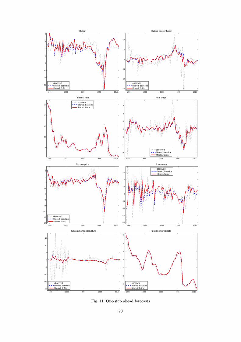
4.5 Forecasting performance

Figures 11 to 13 show one-step ahead forecasts of the baseline and the financial frictions models for allthe observables. These are not true out-of-sample forecasts because the model is calibrated/estimated onthe whole sample period 1995Q1-2012Q4. Nevertheless, these figures indicate approximate forecastingperformance of the models. Particularly, it is informative to see whether the models tend to yield unbiasedforecasts. The results show that the models forecast relatively well. No crucial biases are evident, exceptfor the CPI inflation which appears to be slightly upward biased. The total hours worked forecasts arerather volatile, inducing this volatility in the GDP series.

Table 6 reports the forecasting performance of the baseline and financial frictions models relative toa random walk model (in terms of quarterly growth rates) with respect to predicting CPI inflation andGDP growth for horizons: one, four, eight and 12 quarters. I also report the forecasting performanceof a Bayesian SVAR on three domestic variables: GDP, CPI and nominal interest rate (with the samestructure as the foreign SVAR, and with similar priors), since it is often taken as a benchmark in theliterature15. Table 6 shows that both models forecast both variables at least as precisely as the randomwalk model at all horizons considered. Both models outperform the random walk by about 30% inforecasting both variables for horizons two to three years, and deliver about the same precision at aone quarter horizon. Moreover, the financial frictions model tends to deliver somewhat more preciseforecasts than the baseline model of both CPI inflation and GDP growth, with the forecast differencesbeing statistically significant at shorter horizons in terms of Diebold-Mariano test statistic. Table 6 alsoindicates that the DSGE model does not lose much to the SVAR model in terms of forecasting precision.

Thus, the model can be used not only for policy studies but also for forecasting purposes. The resultsfrom our forecasting exercise are similar to those of CTW who also find that the financial frictions modeltends to outperform the baseline model.

15 The particular SVAR has some economically implausible estimated parameters, since Latvian GDP, CPI inflation andnominal interest rate data do not possess a stable and economically plausible relationship over the particular sample span.

18

ModelDistance 1Q 4Q 8Q 12Qmeasure πc ∆y πc ∆y πc ∆y πc ∆y

BaselineRMSE 1.04 1.01 0.82 0.74 0.67 0.64 0.71 0.64MAE 0.99 1.25 0.86 0.78 0.74 0.63 0.71 0.66

Financialfrictions

RMSE 1.00 0.96 0.78 0.70 0.65 0.64 0.68 0.64DM p-val 0.492 0.319 0.113 0.059 0.101 0.071 0.080 0.091

MAE 0.93 1.15 0.80 0.69 0.70 0.57 0.66 0.60DM p-val 0.279 0.900 0.125 0.025 0.117 0.058 0.070 0.104

SVARRMSE 0.86 0.72 0.71 0.81 0.62 0.68 0.63 0.66MAE 0.89 0.71 0.70 0.77 0.62 0.62 0.58 0.61

Finfric vsBaseline

DM p-val (RMSE) 0.006 0.005 0.018 0.111 0.162 0.451 0.136 0.516

DM p-val (MAE) 0.001 0.000 0.011 0.053 0.069 0.125 0.089 0.090

Table 6: Root mean squared forecast error (RMSE) and mean absolute forecast error (MAE) comparedto the random walk model.

Note: 1) For RMSE and MAE, a number less than unity indicates that the model makes more precise forecasts comparedto the random walk model.2) DM p-val is a one-sided p-value of the Diebold-Mariano (Diebold and Mariano, 1995) test for equal forecast accuracybetween two models. Its value below 0.05 implies that the precision of a model’s forecasts is better than the alternative’sat a 5% significance level. The last row of the table compares the financial frictions model versus baseline model.3) SVAR is estimated on three domestic variables: GDP, CPI and nominal interest rate, and is of the same structure andwith similar priors as the foreign SVAR.4) Note that this is not a true out-of-sample forecasting performance since the models have been estimated on the wholesample period 1995Q1-2012Q4.

19

1996 2000 2004 2008 2012

−10

−8

−6

−4

−2

0

2

4

Output

observedfiltered, baselinefiltered, finfric

1996 2000 2004 2008 2012

−30

−20

−10

0

10

20

Output price inflation


1996 2000 2004 2008 2012

5

10

15

20

25

Interest rate


1996 2000 2004 2008 2012

−6

−4

−2

0

2

4

6

Real wage


1996 2000 2004 2008 2012−14

−12

−10

−8

−6

−4

−2

0

2

4

Consumption


1996 2000 2004 2008 2012

−40

−30

−20

−10

0

10

20

30

Investment


1996 2000 2004 2008 2012

−20

−15

−10

−5

0

5

10

15

Government expenditure


1996 2000 2004 2008 2012

1

2

3

4

5

6

7

Foreign interest rate


Fig. 11: One-step ahead forecasts

20

1996 2000 2004 2008 2012

−5

−4

−3

−2

−1

0

1

2

3

4

5

Real exchange rate


1996 2000 2004 2008 2012

−12

−10

−8

−6

−4

−2

0

2

4

Total hours


1996 2000 2004 2008 2012−16

−14

−12

−10

−8

−6

−4

−2

0

2

4

Exports


1996 2000 2004 2008 2012

−25

−20

−15

−10

−5

0

5

10

15

Imports


1996 2000 2004 2008 2012

−10

−5

0

5

10

15

20

CPI inflation


1996 2000 2004 2008 2012

−100

−50

0

50

100

Investment price inflation


1996 2000 2004 2008 2012

0

0.5

1

1.5

2

2.5

3

3.5

Foreign inflation


1996 2000 2004 2008 2012

−3

−2.5

−2

−1.5

−1

−0.5

0

0.5

Foreign output


Fig. 12: One-step ahead forecasts (continued)

21

1996 2000 2004 2008 2012

−40

−30

−20

−10

0

10

20

Net worth


1996 2000 2004 2008 2012

1

2

3

4

5

6

7

8

9

10

11

Spread


Fig. 13: One-step ahead forecasts (continued)

5 Summary and conclusions

This paper builds a DSGE model for Latvia that would be suitable to replace the traditional macro-econometric model currently employed as the main macroeconomic model at Bank of Latvia. For thatpurpose, I adapt the Christiano, Trabandt and Walentin (2011, henceforth CTW) financial frictionsmodel to Latvia’s data. The monetary policy is modeled as a currency union. I study whether addingthe financial frictions block to an otherwise identical (‘baseline’) model is an improvement with respectto several dimensions.

The main findings are as follows. The addition of financial frictions block provides more appealinginterpretation for the drivers of economic activity, and allows to reinterpret their role. Financial frictionsplayed an important part in Latvia’s 2008-recession. The financial frictions model beats both the baselinemodel and the random walk model in forecasting both CPI inflation and GDP, and does not lose muchto a SVAR.

Overall, the results suggest that the financial frictions model is suitable for both policy analysis andforecasting exercises, and is an improvement over the model without the financial frictions block.

This paper employs a model of financial frictions for firms but abstracts from frictions in financinghouseholds. In the future work, it would be beneficial to separate frictions in the two markets.

Acknowledgements I thank Viktors Ajevskis, Rudolfs Bems, Konstantins Benkovskis, Martins Bitans, Dmitry Kulikov,Karl Walentin and two anonymous referees for feedback. I also thank Andrejs Kurbatskis and several other colleagues atBank of Latvia for helping with the data. All remaining errors are my own.

I have benefited from the program code provided by Lawrence Christiano, Mathias Trabandt and Karl Walentin fortheir model.

References

1. Adjemian S, Bastani H, Juillard M, Karame F, Mihoubi F, Perendia G, Pfeifer J, Ratto M, Villemot S (2011) Dynare:Reference Manual, Version 4. Dynare Working Papers, 1, CEPREMAP

2. Adolfson M, Laseen S, Linde J, Villani M (2008) Evaluating an estimated new Keynesian small open economy model.J Econ Dyn Control 32:2690-2721. doi: 10.1016/j.jedc.2007.09.012

3. Bernanke B, Gertler M, Gilchrist S (1999) The financial accelerator in a quantitative business cycle framework.In: Taylor JB, Woodford M (ed) Handbook of Macroeconomics, Elsevier Science, 1341-1393. doi: 10.1016/S1574-0048(99)10034-X

4. Christiano LJ, Eichenbaum M, Evans CL (2005) Nominal rigidities and the dynamic effects of a shock to monetarypolicy. J POLIT ECON 113:1-45. doi: 10.1086/426038

5. Christiano, LJ, Motto R, Rostagno M (2014) Risk shocks. Am Econ Rev 104:27-65. doi:10.1257/aer.104.1.276. Christiano LJ, Trabandt M, Walentin K (2010) Involuntary unemployment and the business cycle. NBER Working

Papers 15801, National Bureau of Economic Research, Inc.7. Christiano LJ, Trabandt M, Walentin K (2011) Introducing financial frictions and unemployment into a small open

economy model. J Econ Dyn Control 35:1999-2041. doi: 10.1016/j.jedc.2011.09.0058. Diebold FX, Mariano R (1995) Comparing predictive accuracy. J Bus Econ Stat 13:253-265.9. Dixit AK, Stiglitz JE (1977) Monopolistic competition and optimum product diversity. Am Econ Rev 67:297-308

22

10. Erceg CJ, Dale WH, Levin AT (2000) Optimal monetary policy with staggered wage and price contracts. J MonetaryEcon 46:281-313. doi: 10.1016/S0304-3932(00)00028-3

11. Fisher I (1933) The debt-deflation theory of great depressions. Econometrica 1:337-35712. Justiniano A, Primiceri G, Tambalotti A (2011) Investment shocks and the relative price of investment. Rev Econ

Dynamics 14:101-121. doi: 10.1016/j.red.2010.08.00413. Stehrer R (2013) Accounting relations in bilateral value added trade. wiiw Working Papers 101, The Vienna Institute

for International Economic Studies, wiiw

23

Table 3: Estimated domestic block parameters

DescriptionPrior Posterior HPD int.

Distr. Mean st.d.Mean st.d. 5% 95%

base finfric base finfric finfric

ξd Calvo, domestic β 0.75 0.075 0.800 0.804 0.025 0.023 0.756 0.860ξx Calvo, exports β 0.75 0.075 0.848 0.860 0.034 0.031 0.806 0.910ξmc Calvo, imports for consumpt. β 0.75 0.075 0.774 0.779 0.042 0.049 0.676 0.898ξmi Calvo, imports for investment β 0.65 0.075 0.556 0.408 0.062 0.042 0.306 0.525ξmx Calvo, imports for exports β 0.65 0.10 0.546 0.589 0.082 0.091 0.452 0.731κd Indexation, domestic β 0.40 0.15 0.196 0.162 0.066 0.075 0.037 0.303κx Indexation, exports β 0.40 0.15 0.308 0.301 0.086 0.107 0.108 0.506κmc Indexation, imports for cons. β 0.40 0.15 0.357 0.366 0.114 0.106 0.156 0.610κmi Indexation, imports for inv. β 0.40 0.15 0.286 0.249 0.115 0.100 0.052 0.461κmx Indexation, imports for exp. β 0.40 0.15 0.299 0.317 0.095 0.115 0.094 0.534κw Indexation, wages β 0.40 0.15 0.258 0.241 0.091 0.079 0.062 0.447νj Working capital share β 0.50 0.25 0.381 0.456 0.253 0.179 0.017 0.882

0.1σL Inverse Frisch elasticity Γ 0.30 0.15 0.199 0.287 0.094 0.106 0.083 0.541b Habit in consumption β 0.65 0.15 0.854 0.898 0.043 0.030 0.839 0.9540.1S′′ Investment adjustment costs Γ 0.50 0.15 0.414 0.168 0.077 0.030 0.094 0.254σa Variable capital utilization Γ 0.20 0.075 0.375 0.567 0.091 0.093 0.291 0.855ηx Elasticity of subst., exports Γtr 1.50 0.25 1.681 1.535 0.162 0.143 1.098 1.959ηc Elasticity of subst., cons. Γtr 1.50 0.25 1.444 1.333 0.163 0.164 1.023 1.678ηi Elasticity of subst., invest. Γtr 1.50 0.25 1.122 1.1∗ 0.067ηf Elasticity of subst., foreign Γtr 1.50 0.25 1.544 1.540 0.206 0.159 1.085 2.036µ Monitoring cost β 0.30 0.075 0.273 0.040 0.188 0.352

ρε Persistence, stationary tech. β 0.85 0.075 0.883 0.847 0.038 0.041 0.724 0.953ρΥ Persistence, MEI β 0.85 0.075 0.803 0.588 0.059 0.106 0.340 0.851ρζc Persist., consumption prefs β 0.85 0.075 0.852 0.851 0.053 0.038 0.733 0.945ρζh Persistence, labor prefs β 0.85 0.075 0.801 0.817 0.083 0.048 0.694 0.935

ρφ̃ Persist., country risk prem. β 0.85 0.075 0.912 0.934 0.024 0.025 0.884 0.976

ρg Persist., gov. expenditures β 0.85 0.075 0.762 0.777 0.051 0.083 0.627 0.930ργ Persistence, entrepren. wealth β 0.85 0.075 0.796 0.059 0.634 0.951

Standard deviations of shocks

10σε Stationary technology Inv-Γ 0.15 inf 0.139 0.126 0.015 0.014 0.098 0.155σΥ Marginal efficiency of invest. Inv-Γ 0.15 inf 0.236 0.157 0.038 0.027 0.066 0.255σζc Consumption prefs Inv-Γ 0.15 inf 0.152 0.236 0.049 0.056 0.123 0.373σζh Labor prefs Inv-Γ 0.50 inf 0.708 0.895 0.415 0.283 0.269 1.740

100σφ̃ Country risk premium Inv-Γ 0.50 inf 0.544 0.552 0.044 0.045 0.460 0.652

10σg Government expenditures Inv-Γ 0.50 inf 0.465 0.471 0.046 0.041 0.380 0.565στd Markup, domestic Inv-Γ 0.50 inf 0.368 0.373 0.107 0.089 0.183 0.625στx Markup, exports Inv-Γ 0.50 inf 0.852 0.992 0.332 0.391 0.428 1.670στm,c Markup, imports for cons. Inv-Γ 0.50 inf 0.878 0.863 0.334 0.329 0.192 1.915στm,i Markup, imports for invest. Inv-Γ 0.50 inf 0.911 0.433 0.319 0.078 0.263 0.622στm,x Markup, imports for exports Inv-Γ 0.50 inf 1.306 1.383 0.501 0.643 0.540 2.38510σγ Entrepreneurial wealth Inv-Γ 0.50 inf 0.295 0.042 0.215 0.381

Model fit items

base finfricLog marginal likelihood∗∗ -2959.4 -2925.9Posterior odds ratio base : finfric∗∗ 1 : 3.5e14

Note: Based on two Metropolis-Hastings chains, each with 50 000 draws after a burn-in period of 200 000 draws.Truncated priors, denoted by Γtr, with no mass below 1.01 have been used for the elasticity parameters ηj , j = {x, c, i, f}.∗ Calibrated in order to avoid numerical issues.∗∗ To compare marginal likelihood across the models, a common set of observables and estimated parameters are used.Specifically, the interest rate spread and the stock market growth data are excluded from the observables in the financialfrictions model, and the otherwise estimated parameters particular to the financial accelerator block are calibrated to theirposterior mean values.

24

Financial frictions in Latvia -...

Documents

Transcript of Financial frictions in Latvia -...