FINANCIAL FRICTIONS IN A DSGE MODEL FOR LATVIA · 2018-11-20 · 4 FINANCIAL FRICTIONS IN A DSGE...
85
Transcript of FINANCIAL FRICTIONS IN A DSGE MODEL FOR LATVIA · 2018-11-20 · 4 FINANCIAL FRICTIONS IN A DSGE...

1
F I N A N C I A L F R I C T I O N S I N A D S G E M O D E L F O R L A T V I A
CONTENTS ABSTRACT 2 INTRODUCTION 3 1. MODEL IN BRIEF 4
1.1 Baseline model 4 1.2 Financial frictions model 5
2. ESTIMATION 5 2.1 Calibration 5 2.2 Priors 8 2.3 Data 8 2.4 Shocks and measurement errors 8
3. RESULTS 9 3.1 Posterior parameter values 9 3.2 Model moments and variance decomposition 12 3.3 Impulse response functions 18 3.4 Smoothed shock values and historical decomposition 22 3.5 Forecasting performance 29
4. CONCLUSIONS 33 APPENDICES 34 BIBLIOGRAPHY 84
ABBREVIATIONS
ABP – annualised basis points AR(1) – first-order autoregression BGG – Bernanke, Gertler and Gilchrist (1999) CPI – consumer price index CTW – Christiano, Trabandt and Walentin (2011) dev. – deviation distr. – distribution DSGE – dynamic stochastic general equilibrium ECFIN – Directorate General for Economic and Financial Affairs finfric – financial frictions FOC – first order condition HPD – highest posterior density i.i.d. – independent and identically distributed IRF – impulse response functions MAE – mean absolute error MEI – marginal efficiency of investment pp – percentage point RMSE – root mean squared error SVAR – structural vector autoregression St.d. – standard deviation wiiw – Vienna Institute for International Economic Studies

2
F I N A N C I A L F R I C T I O N S I N A D S G E M O D E L F O R L A T V I A
ABSTRACT
This paper builds a dynamic stochastic general equilibrium (DSGE) model for Latvia that would be suitable for policy analysis and forecasting purposes at Latvijas Banka. For that purpose, the DSGE model with financial frictions of Christiano, Trabandt and Walentin (2011) is adapted to Latvia's data, estimated, and studied as to whether adding the financial frictions block to an otherwise identical (baseline) model is an improvement with respect to several dimensions. The main findings are: 1) adding of financial frictions block provides a more appealing interpretation for the drivers of economic activity and allows reinterpreting their role; 2) financial frictions played an important part in Latvia's 2008 recession; 3) the financial frictions model beats both the baseline model and the random walk model in forecasting CPI inflation and GDP, and performs roughly the same as a Bayesian structural vector autoregression.
Keywords: DSGE model, financial frictions, small open economy, Bayesian estimation, currency union
JEL codes: E0, E3, F0, F4, G0, G1
I thank Viktors Ajevskis, Rūdolfs Bēms, Konstantīns Beņkovskis, Mārtiņš Bitāns, Dmitry Kulikov and Karl Walentin for feedback. I also thank Andrejs Kurbatskis and several other colleagues at Latvijas Banka for helping with the data. All remaining errors are my own. I have benefited from the programme code provided by Lawrence Christiano, Mathias Trabandt and Karl Walentin for their model.
Disclaimer: This paper is released to inform interested parties of research and to encourage discussion. The views expressed in this paper are those of the author and do not necessarily reflect the views of Latvijas Banka.

3
F I N A N C I A L F R I C T I O N S I N A D S G E M O D E L F O R L A T V I A
INTRODUCTION
This paper is an attempt to build a dynamic stochastic general equilibrium (DSGE) model for Latvia that would be suitable for policy analysis and forecasting purposes at Latvijas Banka, since the current main macroeconomic model lacks microeconomic foundations. Also, the recent financial crisis has suggested that business cycle modelling should not abstract from financial factors, thus modelling financial frictions is deemed to be requisite.
Therefore, I take the model of Lawrence Christiano, Mathias Trabandt and Karl Walentin (2011) (henceforth, CTW) with financial frictions as a starting point. To assess the effect of having financial frictions mechanism in a DSGE model, I compare the output of the model throughout the paper with an otherwise identical model, called the baseline model but lacking the mechanism of financial frictions. The baseline model is a standard open economy model, and it builds on Christiano, Eichenbaum and Evans (2005) and Adolfson, Laseén, Lindé and Villani (2008). The financial frictions model adds the Bernanke, Gertler and Gilchrist (1999), (henceforth, BGG) financial accelerator mechanism to the baseline model.
The CTW model is modified with respect to monetary policy: since Latvia's currency had been pegged to the euro since 2005 and in 2014, when Latvia joined the euro area, was replaced by the euro, monetary policy is modelled as nominal interest rate peg to foreign interest rate. The foreign economy is modelled as a Bayesian structural vector autoregression (SVAR) in foreign output, inflation, nominal interest rate and technology growth.
The main findings are as follows: 1) adding of financial frictions block provides a more appealing interpretation for the drivers of economic activity and allows reinterpreting their role; 2) financial frictions played an important part in Latvia's 2008 recession; 3) the financial frictions model beats both the baseline model and the random walk model in forecasting CPI inflation and GDP.
The paper is structured as follows. Section 1 overviews the model. Section 2 describes the estimation procedure, and Section 3 deals with the results. Section 4 concludes. Appendix A contains further computational results. Appendices B and C contain a detailed description of the model.
4
F I N A N C I A L F R I C T I O N S I N A D S G E M O D E L F O R L A T V I A
1. MODEL IN BRIEF
Since the model is almost a replica of the CTW model (2011), this Section is a brief introduction to the model, whereas its formal description is relegated to Appendix B. The only noticeable difference between the CTW model and this one is in the behavior of monetary authority, which is modelled as an interest rate peg in this paper.
1.1 Baseline model
The baseline model builds on Christiano, Eichenbaum and Evans (2005), and Adolfson, Laséen, Lindé and Villani (2008). The three final goods, i.e. consumption, investment and exports, are produced by combining the domestic homogeneous good with specific imported inputs for each type of final good. Specialised domestic importers purchase a homogeneous foreign good, which they turn into a specialised input and sell to domestic import retailers. There are three types of import retailers: one uses these specialised import goods to create a homogeneous good used as an input into the production of specialised exports; the other uses these specialised import goods to create an input used in the production of investment goods, while the third uses specialised imports to produce homogeneous input used in the production of consumption goods. Exports involve a Dixit-Stiglitz (Dixit and Stiglitz (1977)) continuum of exporters, each of which is a monopolist that produces a specialised export good. Each monopolist produces its export good using a homogeneous, domestically produced good and a homogeneous good derived from imports. The homogeneous domestic good is produced by a competitive, representative firm. The domestic good is allocated among 1) government consumption (which consists entirely of the domestic good), 2) production of consumption goods, 3) production of investment goods, and 4) production of export goods. A part of the domestic good is lost due to the real friction in the model economy due to investment adjustment and capital utilisation costs. Households maximise expected utility from a discounted stream of consumption (subject to habit) and hours worked. In the baseline model, households own the economy's stock of physical capital. They determine the rate at which capital stock is accumulated and the rate at which it is utilised. Households also own the stock of net foreign assets and determine the rate of its accumulation.
Monetary policy is conducted as a hard peg of the domestic nominal interest rate to the foreign nominal interest rate1. Government expenditures change exogenously. Taxes in the model economy are the capital tax, payroll tax, consumption tax, labour income tax, and bond tax. Any difference between government expenditures and tax revenue is offset by lump-sum transfers. The foreign economy is modelled as a Bayesian SVAR in foreign output, inflation, nominal interest rate and technology growth. The model economy has two sources of exogenous growth: the neutral technology growth and the investment-specific technology growth.
1 A generalised Taylor rule, including foreign interest rate and nominal exchange rate, was also studied but the results are skipped due to the space constraint. In short, the peg system fits the data better.
5
F I N A N C I A L F R I C T I O N S I N A D S G E M O D E L F O R L A T V I A
1.2 Financial frictions model
The details are relegated to Appendix B, while a brief summary of the model follows herein. The financial frictions model adds the BGG (1999) financial frictions to the above baseline model. Financial frictions suggest that borrowers and lenders are different people, and that they have different information. Thus the model introduces "entrepreneurs" or agents who have special skills in the operation and management of capital. Their skill in operating capital is such that it is optimal for them to operate more capital than their own resources can support by borrowing additional funds. There is some financial friction, because managing capital is risky, i.e. entrepreneurs can go bankrupt, and only the entrepreneurs costlessly observe their own idiosyncratic productivity. In this model, it is the households that deposit money in banks. The interest rate that households receive is nominally non state-contingent.2 Banks then lend funds to entrepreneurs using a standard nominal debt contract, which is optimal given the asymmetric information.3 The amount that banks are willing to lend to an entrepreneur under a debt contract is a function of the respective entrepreneur's net worth. This is how balance sheet constraints enter the model. When a shock that reduces the value of entrepreneurs' assets occurs, this cuts into their ability to borrow. As a result, entrepreneurs acquire less capital, and this translates into a reduction in investment and leads to a slowdown in the economy. Although individual entrepreneurs are risky, banks are not.
The financial frictions block brings in two new endogenous variables, one related to the interest rate paid by entrepreneurs and the other associated with their net worth. There are also two new shocks – one to idiosyncratic uncertainty and the other to entrepreneurial wealth.
The explicit description of both baseline and financial frictions models is relegated to Appendix B.
2. ESTIMATION
Both the baseline and financial frictions models are estimated with the Bayesian techniques. The equilibrium conditions of the model are reported in Appendix C.
2.1 Calibration
The time unit is a quarter. A subset of model parameters is calibrated and the rest are estimated using the data for Latvia and the euro area. The calibrated values are displayed in Tables 1 and 2. These are the parameters that are typically calibrated in the literature and are related to "great ratios" and other observable quantities associated with steady state values. The values of the parameters are selected such that they would be specific to the data at hand. Sample averages are used when available. The discount factor and the tax rate on bonds are set to match
2 These nominal contracts give rise to wealth effects of unexpected changes in the price level, as emphasised by Fisher (1933). For instance, in the case of a shock driving the price level down, households receive a wealth transfer. This transfer is taken from entrepreneurs whose net worth is thereby reduced. With the tightening of their balance sheets, the ability of entrepreneurs to invest is reduced, and this generates an economic slowdown. 3 Namely, the equilibrium debt contract maximises the expected entrepreneurial welfare, subject to the zero profit condition on banks and the specified return on household bank liabilities.
6
F I N A N C I A L F R I C T I O N S I N A D S G E M O D E L F O R L A T V I A
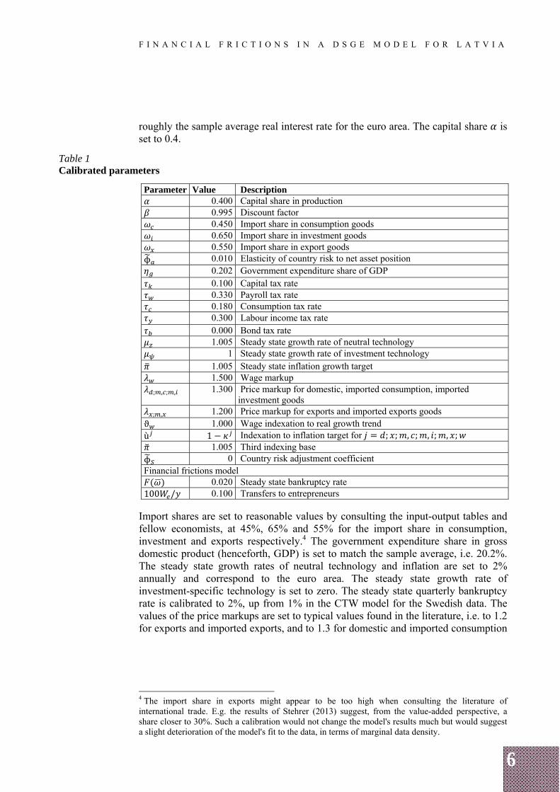
roughly the sample average real interest rate for the euro area. The capital share is set to 0.4.
Table 1 Calibrated parameters
Parameter Value Description 0.400 Capital share in production 0.995 Discount factor 0.450 Import share in consumption goods 0.650 Import share in investment goods 0.550 Import share in export goods
ϕ 0.010 Elasticity of country risk to net asset position 0.202 Government expenditure share of GDP 0.100 Capital tax rate 0.330 Payroll tax rate 0.180 Consumption tax rate 0.300 Labour income tax rate 0.000 Bond tax rate 1.005 Steady state growth rate of neutral technology 1 Steady state growth rate of investment technology
1.005 Steady state inflation growth target 1.500 Wage markup
; , ; , 1.300 Price markup for domestic, imported consumption, imported investment goods
; , 1.200 Price markup for exports and imported exports goods ϑ 1.000 Wage indexation to real growth trend ù 1 Indexation to inflation target for ; ; , ; , ; , ;
1.005 Third indexing base ϕ 0 Country risk adjustment coefficient Financial frictions model
0.020 Steady state bankruptcy rate 100 / 0.100 Transfers to entrepreneurs
Import shares are set to reasonable values by consulting the input-output tables and fellow economists, at 45%, 65% and 55% for the import share in consumption, investment and exports respectively.4 The government expenditure share in gross domestic product (henceforth, GDP) is set to match the sample average, i.e. 20.2%. The steady state growth rates of neutral technology and inflation are set to 2% annually and correspond to the euro area. The steady state growth rate of investment-specific technology is set to zero. The steady state quarterly bankruptcy rate is calibrated to 2%, up from 1% in the CTW model for the Swedish data. The values of the price markups are set to typical values found in the literature, i.e. to 1.2 for exports and imported exports, and to 1.3 for domestic and imported consumption
4 The import share in exports might appear to be too high when consulting the literature of international trade. E.g. the results of Stehrer (2013) suggest, from the value-added perspective, a share closer to 30%. Such a calibration would not change the model's results much but would suggest a slight deterioration of the model's fit to the data, in terms of marginal data density.
7
F I N A N C I A L F R I C T I O N S I N A D S G E M O D E L F O R L A T V I A
as well as imported investment, which is supported by the model's fit in terms of marginal data density5. Wage markup is set to 1.5 as in CTW.
There is full indexation of wages to the steady state real growth ϑ = 1. The other indexation parameters are set to get full indexation and thereby to avoid steady state price and wage dispersion, following CTW. Tax rates are calibrated such that they would represent implicit or effective rates. Three of them are calibrated using the Eurostat data6: the tax rate on capital income is set to 0.1, while the value-added tax on consumption and the personal income tax rate that applies to labour are set to = 0.18 and = 0.3 respectively. The payroll tax rate is set to = 0.33, down from the official 0.35 (0.24 by employer and 0.11 by employee). The elasticity of country risk to net asset position ϕ is set to a small positive number, and in that region its purpose is to induce a unique steady state for the net foreign asset position. Transfers to entrepreneurs' parameter / are kept the same as in CTW. The country risk adjustment coefficient in the uncovered interest parity condition is set to zero in order to impose the nominal interest rate peg.
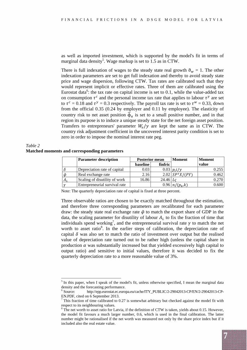
Table 2 Matched moments and corresponding parameters
Parameter description Posterior mean Moment Moment value baseline finfric
Depreciation rate of capital 0.03 0.03 / 0.255 Real exchange rate 2.16 2.02 /( ) 0.462 Scaling of disutility of work 16.86 24.46 0.270
Entrepreneurial survival rate 0.96 /( ) 0.600
Note: The quarterly depreciation rate of capital is fixed at three percent. Three observable ratios are chosen to be exactly matched throughout the estimation, and therefore three corresponding parameters are recalibrated for each parameter draw: the steady state real exchange rate to match the export share of GDP in the data, the scaling parameter for disutility of labour to fix the fraction of time that individuals spend working7, and the entrepreneurial survival rate to match the net worth to asset ratio8. In the earlier steps of calibration, the depreciation rate of capital was also set to match the ratio of investment over output but the realised value of depreciation rate turned out to be rather high (unless the capital share in production was substantially increased but that yielded excessively high capital to output ratio) and sensitive to initial values, therefore it was decided to fix the quarterly depreciation rate to a more reasonable value of 3%.
5 In this paper, when I speak of the model's fit, unless otherwise specified, I mean the marginal data density and the forecasting performance. 6 Source: http://epp.eurostat.ec.europa.eu/cache/ITY_PUBLIC/2-29042013-CP/EN/2-29042013-CP-EN.PDF, cited on 6 September 2013. 7 This fraction of time calibrated to 0.27 is somewhat arbitrary but checked against the model fit with respect to its neighbouring values. 8 The net worth to asset ratio for Latvia, if the definition of CTW is taken, yields about 0.15. However, the model fit favours a much larger number, 0.6, which is used in the final calibration. The latter number might be rationalised if the net worth was measured not only by the share price index but if it included also the real estate value.
8
F I N A N C I A L F R I C T I O N S I N A D S G E M O D E L F O R L A T V I A
2.2 Priors
There are 21 structural parameters, eight first-order autoregressive (henceforth, AR(1)) coefficients, 16 Bayesian SVAR parameters for the foreign economy, and 16 shock standard deviations estimated with the Bayesian techniques within Matlab/Dynare environment (Adjemian et al. (2011)). The priors are displayed in Tables 3 to 6. The priors are similar to CTW. Less agnostic priors are assigned for the foreign Bayesian SVAR model, since otherwise the foreign monetary policy appears to be weakly identified9. The prior means of the estimated standard deviations are set closer to their posteriors, and parameters and shock standard deviations are scaled to be of similar order of magnitude in order to facilitate optimisation.
2.3 Data
The model is estimated using data for Latvia (the domestic part) and the euro area (the foreign part). The sample period is 1995 Q1–2012 Q4. 18 observable time series are used to estimate the financial frictions model and two less to estimate the baseline model. The variables used in levels are the nominal interest rate, GDP deflator inflation, CPI inflation, investment price index inflation, foreign CPI inflation, foreign nominal interest rate and interest rate spread. The rest of the variables are in terms of first differences of logs, and they are GDP, consumption, investment, exports, imports, government expenditures, real wages, real exchange rate, real stock prices, total hours worked, and foreign GDP. All of the differenced variables are demeaned, except for total hours worked. The domestic inflation rates and the real exchange rate are demeaned as well. All of the real quantities are in per capita terms. All foreign variables correspond to the euro area data.
2.4 Shocks and measurement errors
In total, there are 18 exogenous stochastic variables in the theoretical financial frictions model. There are four technology shocks (stationary neutral technology , stationary marginal efficiency of investment Υ, unit-root neutral technology , and unit-root investment specific technology ), a shock to consumption preferences and to disutility of labour supply , a shock to government expenditure , and a country risk premium shock that affects the relative riskiness of foreign assets compared to domestic assets ϕ. There are five markup shocks, one for each type of intermediate good, , , , , , , , ( – domestic, – exports, , – imported consumption, , – imported investment, , – imported exports). The financial frictions model has two more shocks – one to idiosyncratic uncertainty , and one to entrepreneurial wealth . There are also shocks to each of the observed foreign variables: foreign GDP ∗, foreign inflation ∗, and foreign nominal interest rate ∗.
9 Unreported results show that this is true regardless of the sample span used in the estimation and whether or not the foreign block is estimated separately from the domestic block. Also, the use of foreign CPI inflation instead of foreign GDP deflator's inflation (which is used by CTW) improves the identification of foreign monetary policy only marginally. Therefore, the results involving foreign monetary policy should be interpreted with caution. The replacement of foreign Bayesian SVAR with a full-fledged foreign DSGE block thus might be an improvement but is not considered in this paper.
9
F I N A N C I A L F R I C T I O N S I N A D S G E M O D E L F O R L A T V I A
The stochastic structure of exogenous variables is the following: eight of these evolve according to AR(1) processes:
, Υ , , , , ϕ , , .
Five shock processes are i.i.d.:
, , , , , , , ,
and five shock processes are assumed to follow a first-order SVAR:
∗, ∗, ∗, , , , .
As in CTW, two shocks are suspended in the estimation: the shock to unit-root investment specific technology , and the idiosyncratic entrepreneur risk shock . The first one should correspond to the foreign block but its identification is dubious in the particular SVAR model; the second has been found to have limited importance in CTW.
There are measurement errors, except for domestic interest rate and the foreign variables. The variance of measurement errors is calibrated to correspond to 10% of the variance of each data series.
3. RESULTS
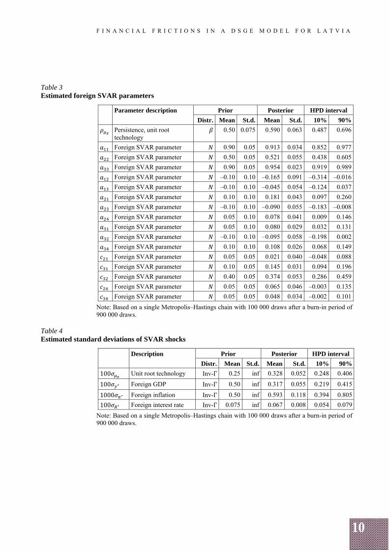
The domestic and foreign blocks are estimated separately since Latvia's economy has minuscule effect on the euro area. The estimation results for the foreign SVAR model are obtained using a single Metropolis–Hastings chain with 100 000 draws after a burn-in of 900 000 draws. For the domestic block, the estimation results are obtained using a single Metropolis–Hastings chain with 100 000 draws after a burn-in of 400 000 draws. Prior-posterior plots are shown in Appendix A.
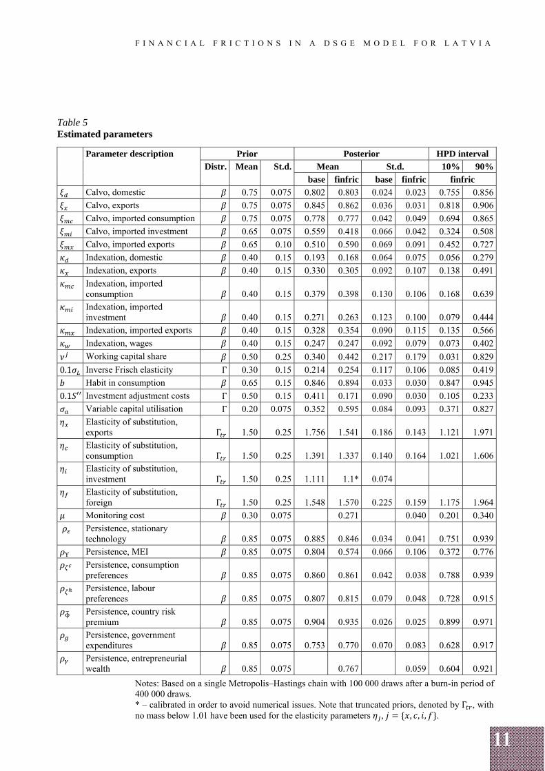
3.1 Posterior parameter values
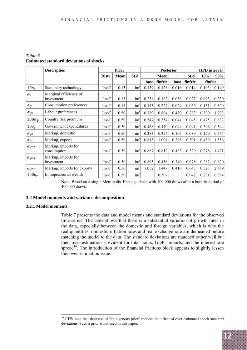
Posterior parameter estimates for the foreign block are reported in Tables 3 and 4, and those specific to the domestic block are shown in Tables 5 and 6. The priors were deliberately fixed to be the same across the two models for a more transparent comparison and favor the baseline model. The estimated mode of elasticity of substitution of the investment goods parameter is close to unity, and thus the parameter is calibrated for the financial frictions model to 1.1, similar to the posterior mean in the baseline model, in order to avoid numerical issues. Overall, the estimated posterior means of parameters are similar between the two models. The most notable difference is in the investment adjustment costs parameter, which is about 2.4 times lower for the financial frictions model compared to the baseline specification. They are statistically significantly different at 10% significance level. The lower parameter indicates that the financial frictions model induces the gradual response, which the investment adjustment mechanism was introduced to generate. Also, the estimated persistence parameter of the marginal efficiency of investment (MEI) shock is reduced (from 0.80 to 0.57) with the introduction of the financial frictions block. Regarding the estimated standard deviations of shocks, the financial frictions model assigns a smaller standard deviation to the marginal efficiency of investment shock, which, apparently, is "crowded out" by the entrepreneurial wealth shock.
10
F I N A N C I A L F R I C T I O N S I N A D S G E M O D E L F O R L A T V I A
Table 3 Estimated foreign SVAR parameters
Parameter description Prior Posterior HPD interval
Distr. Mean St.d. Mean St.d. 10% 90%
Persistence, unit root technology
0.50 0.075 0.590 0.063 0.487 0.696
Foreign SVAR parameter 0.90 0.05 0.913 0.034 0.852 0.977
Foreign SVAR parameter 0.50 0.05 0.521 0.055 0.438 0.605
Foreign SVAR parameter 0.90 0.05 0.954 0.023 0.919 0.989
Foreign SVAR parameter –0.10 0.10 –0.165 0.091 –0.314 –0.016
Foreign SVAR parameter –0.10 0.10 –0.045 0.054 –0.124 0.037
Foreign SVAR parameter 0.10 0.10 0.181 0.043 0.097 0.260
Foreign SVAR parameter –0.10 0.10 –0.090 0.055 –0.183 –0.008
Foreign SVAR parameter 0.05 0.10 0.078 0.041 0.009 0.146
Foreign SVAR parameter 0.05 0.10 0.080 0.029 0.032 0.131
Foreign SVAR parameter –0.10 0.10 –0.095 0.058 –0.198 0.002
Foreign SVAR parameter 0.10 0.10 0.108 0.026 0.068 0.149
Foreign SVAR parameter 0.05 0.05 0.021 0.040 –0.048 0.088
Foreign SVAR parameter 0.10 0.05 0.145 0.031 0.094 0.196
Foreign SVAR parameter 0.40 0.05 0.374 0.053 0.286 0.459
Foreign SVAR parameter 0.05 0.05 0.065 0.046 –0.003 0.135
Foreign SVAR parameter 0.05 0.05 0.048 0.034 –0.002 0.101
Note: Based on a single Metropolis–Hastings chain with 100 000 draws after a burn-in period of 900 000 draws.
Table 4 Estimated standard deviations of SVAR shocks
Description Prior Posterior HPD interval
Distr. Mean St.d. Mean St.d. 10% 90%
100 Unit root technology Inv-Γ 0.25 inf 0.328 0.052 0.248 0.406
100 ∗ Foreign GDP Inv-Γ 0.50 inf 0.317 0.055 0.219 0.415
1000 ∗ Foreign inflation Inv-Γ 0.50 inf 0.593 0.118 0.394 0.805
100 ∗ Foreign interest rate Inv-Γ 0.075 inf 0.067 0.008 0.054 0.079
Note: Based on a single Metropolis–Hastings chain with 100 000 draws after a burn-in period of 900 000 draws.
11
F I N A N C I A L F R I C T I O N S I N A D S G E M O D E L F O R L A T V I A
Table 5 Estimated parameters
Parameter description Prior Posterior HPD interval
Distr. Mean St.d. Mean St.d. 10% 90%
base finfric base finfric finfric
Calvo, domestic 0.75 0.075 0.802 0.803 0.024 0.023 0.755 0.856
Calvo, exports 0.75 0.075 0.845 0.862 0.036 0.031 0.818 0.906
Calvo, imported consumption 0.75 0.075 0.778 0.777 0.042 0.049 0.694 0.865
Calvo, imported investment 0.65 0.075 0.559 0.418 0.066 0.042 0.324 0.508
Calvo, imported exports 0.65 0.10 0.510 0.590 0.069 0.091 0.452 0.727
Indexation, domestic 0.40 0.15 0.193 0.168 0.064 0.075 0.056 0.279
Indexation, exports 0.40 0.15 0.330 0.305 0.092 0.107 0.138 0.491
Indexation, imported consumption 0.40 0.15 0.379 0.398 0.130 0.106 0.168 0.639
Indexation, imported investment 0.40 0.15 0.271 0.263 0.123 0.100 0.079 0.444
Indexation, imported exports 0.40 0.15 0.328 0.354 0.090 0.115 0.135 0.566
Indexation, wages 0.40 0.15 0.247 0.247 0.092 0.079 0.073 0.402
Working capital share 0.50 0.25 0.340 0.442 0.217 0.179 0.031 0.829
0.1 Inverse Frisch elasticity Γ 0.30 0.15 0.214 0.254 0.117 0.106 0.085 0.419
Habit in consumption 0.65 0.15 0.846 0.894 0.033 0.030 0.847 0.945
0.1 ′′ Investment adjustment costs Γ 0.50 0.15 0.411 0.171 0.090 0.030 0.105 0.233
Variable capital utilisation Γ 0.20 0.075 0.352 0.595 0.084 0.093 0.371 0.827
Elasticity of substitution, exports Γ 1.50 0.25 1.756 1.541 0.186 0.143 1.121 1.971
Elasticity of substitution, consumption Γ 1.50 0.25 1.391 1.337 0.140 0.164 1.021 1.606
Elasticity of substitution, investment Γ 1.50 0.25 1.111 1.1* 0.074
Elasticity of substitution, foreign Γ 1.50 0.25 1.548 1.570 0.225 0.159 1.175 1.964
Monitoring cost 0.30 0.075 0.271 0.040 0.201 0.340
Persistence, stationary technology 0.85 0.075 0.885 0.846 0.034 0.041 0.751 0.939
Persistence, MEI 0.85 0.075 0.804 0.574 0.066 0.106 0.372 0.776
Persistence, consumption preferences 0.85 0.075 0.860 0.861 0.042 0.038 0.788 0.939
Persistence, labour preferences 0.85 0.075 0.807 0.815 0.079 0.048 0.728 0.915
Persistence, country risk premium 0.85 0.075 0.904 0.935 0.026 0.025 0.899 0.971
Persistence, government expenditures 0.85 0.075 0.753 0.770 0.070 0.083 0.628 0.917
Persistence, entrepreneurial wealth 0.85 0.075 0.767 0.059 0.604 0.921
Notes: Based on a single Metropolis–Hastings chain with 100 000 draws after a burn-in period of 400 000 draws. * – calibrated in order to avoid numerical issues. Note that truncated priors, denoted by Γ , with no mass below 1.01 have been used for the elasticity parameters , , , , .
12
F I N A N C I A L F R I C T I O N S I N A D S G E M O D E L F O R L A T V I A
Table 6 Estimated standard deviations of shocks
Description Prior Posterior HPD interval
Distr. Mean St.d. Mean St.d. 10% 90%
base finfric base finfric finfric
10 Stationary technology Inv-Γ 0.15 inf 0.139 0.126 0.016 0.014 0.103 0.149
Marginal efficiency of investment Inv-Γ 0.15 inf 0.234 0.162 0.056 0.027 0.093 0.230
Consumption preferences Inv-Γ 0.15 inf 0.143 0.227 0.029 0.056 0.131 0.320
Labour preferences Inv-Γ 0.50 inf 0.739 0.804 0.430 0.283 0.300 1.293
100 Country risk premium Inv-Γ 0.50 inf 0.547 0.554 0.044 0.045 0.475 0.632
10 Government expenditures Inv-Γ 0.50 inf 0.468 0.470 0.044 0.041 0.396 0.544
Markup, domestic Inv-Γ 0.50 inf 0.383 0.374 0.105 0.089 0.179 0.555
Markup, exports Inv-Γ 0.50 inf 0.813 1.004 0.298 0.391 0.439 1.556
, Markup, imports for consumption Inv-Γ 0.50 inf 0.887 0.812 0.463 0.329 0.278 1.421
, Markup, imports for investment Inv-Γ 0.50 inf 0.895 0.458 0.340 0.078 0.282 0.620
, Markup, imports for exports Inv-Γ 0.50 inf 1.052 1.447 0.410 0.643 0.523 2.349
100 Entrepreneurial wealth Inv-Γ 0.50 inf 0.307 0.042 0.231 0.384
Note: Based on a single Metropolis–Hastings chain with 100 000 draws after a burn-in period of 400 000 draws.
3.2 Model moments and variance decomposition
3.2.1 Model moments
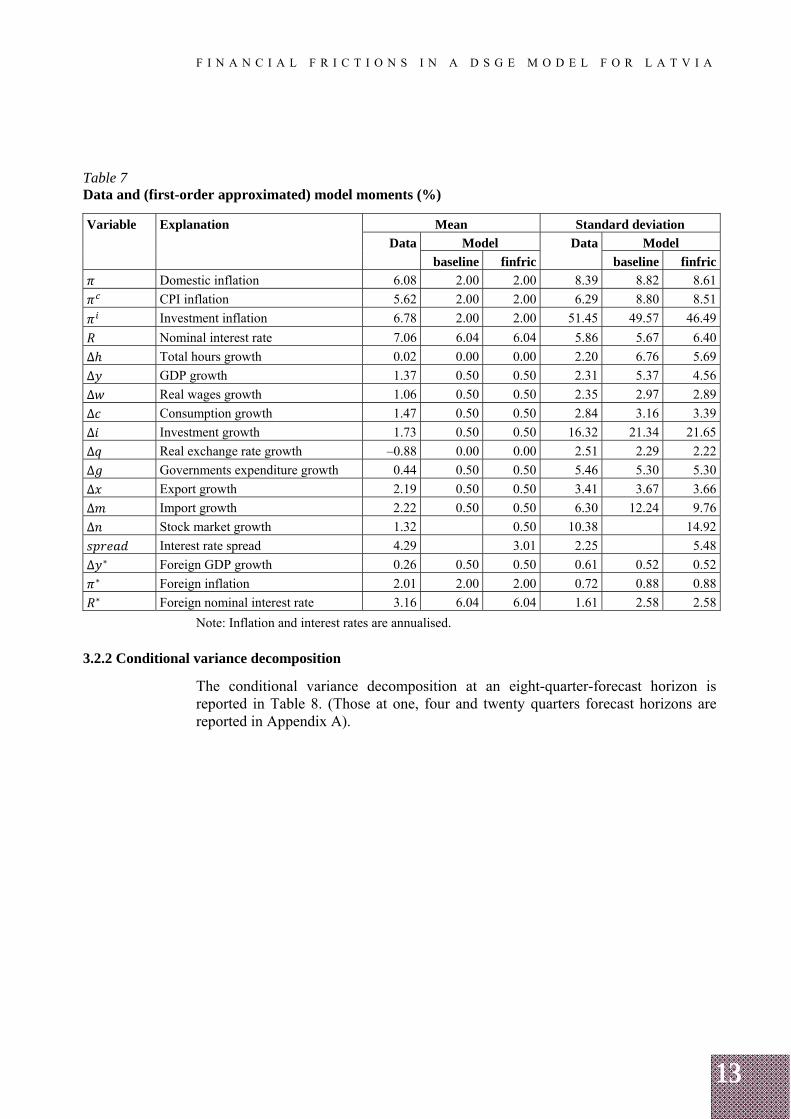
Table 7 presents the data and model means and standard deviations for the observed time series. The table shows that there is a substantial variation of growth rates in the data, especially between the domestic and foreign variables, which is why the real quantities, domestic inflation rates and real exchange rate are demeaned before matching the model to the data. The standard deviations are matched rather well but their over-estimation is evident for total hours, GDP, imports, and the interest rate spread10. The introduction of the financial frictions block appears to slightly lessen this over-estimation issue.
10 CTW note that their use of "endogenous prior" reduces the effect of over-estimated shock standard deviations. Such a prior is not used in this paper.
13
F I N A N C I A L F R I C T I O N S I N A D S G E M O D E L F O R L A T V I A
Table 7 Data and (first-order approximated) model moments (%)
Variable Explanation Mean Standard deviation
Data Model Data Model
baseline finfric baseline finfric
Domestic inflation 6.08 2.00 2.00 8.39 8.82 8.61
CPI inflation 5.62 2.00 2.00 6.29 8.80 8.51
Investment inflation 6.78 2.00 2.00 51.45 49.57 46.49
Nominal interest rate 7.06 6.04 6.04 5.86 5.67 6.40
Δ Total hours growth 0.02 0.00 0.00 2.20 6.76 5.69
Δ GDP growth 1.37 0.50 0.50 2.31 5.37 4.56
Δ Real wages growth 1.06 0.50 0.50 2.35 2.97 2.89
Δ Consumption growth 1.47 0.50 0.50 2.84 3.16 3.39
Δ Investment growth 1.73 0.50 0.50 16.32 21.34 21.65
Δ Real exchange rate growth –0.88 0.00 0.00 2.51 2.29 2.22
Δ Governments expenditure growth 0.44 0.50 0.50 5.46 5.30 5.30
Δ Export growth 2.19 0.50 0.50 3.41 3.67 3.66
Δ Import growth 2.22 0.50 0.50 6.30 12.24 9.76
Δ Stock market growth 1.32 0.50 10.38 14.92
Interest rate spread 4.29 3.01 2.25 5.48
Δ ∗ Foreign GDP growth 0.26 0.50 0.50 0.61 0.52 0.52 ∗ Foreign inflation 2.01 2.00 2.00 0.72 0.88 0.88 ∗ Foreign nominal interest rate 3.16 6.04 6.04 1.61 2.58 2.58
Note: Inflation and interest rates are annualised.
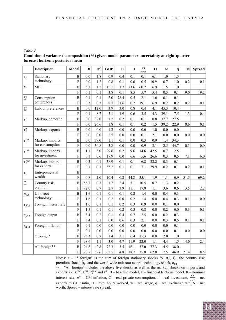
3.2.2 Conditional variance decomposition
The conditional variance decomposition at an eight-quarter-forecast horizon is reported in Table 8. (Those at one, four and twenty quarters forecast horizons are reported in Appendix A).
14
F I N A N C I A L F R I C T I O N S I N A D S G E M O D E L F O R L A T V I A
Table 8 Conditional variance decomposition (%) given model parameter uncertainty at eight-quarter forecast horizon; posterior mean
Description Model GDP C I H w q N Spread
Stationary technology
B 0.0 1.8 0.9 0.4 0.1 0.1 6.1 1.0 1.5
F 0.0 1.2 0.8 0.1 0.0 0.5 10.9 0.7 1.0 0.2 0.1
Υ MEI B 5.1 1.2 15.1 1.7 73.6 60.2 6.9 1.5 1.0
F 0.1 0.1 3.8 0.1 8.5 5.7 5.4 0.5 0.1 19.0 19.2
Consumption preferences
B 0.1 0.1 2.0 78.4 0.5 2.1 1.6 0.1 0.1
F 0.3 0.3 8.7 81.6 0.2 19.1 6.9 0.2 0.2 0.2 0.1
Labour preferences B 0.0 12.0 3.9 3.0 0.8 0.4 4.1 45.3 10.4
F 0.1 8.7 3.1 1.9 0.6 3.5 4.3 39.1 7.5 1.3 0.4
Markup, domestic B 0.0 32.0 1.2 0.2 0.1 0.1 0.8 37.7 27.5
F 0.0 26.6 1.8 0.1 0.1 0.2 1.5 39.2 22.9 0.6 0.1
Markup, exports B 0.0 0.0 1.2 0.0 0.0 0.0 1.0 0.0 0.0
F 0.0 0.0 2.5 0.0 0.0 0.1 2.1 0.0 0.0 0.0 0.0
Markup, imports for consumption
B 0.0 39.0 1.1 0.1 0.0 0.3 0.9 1.4 34.3
F 0.0 50.8 3.8 0.0 0.0 0.9 3.1 2.5 44.7 0.1 0.0
Markup, imports for investment
B 1.1 3.0 29.6 0.2 9.6 14.6 42.5 0.7 2.5
F 0.1 0.6 17.9 0.0 6.6 5.6 26.6 0.3 0.5 7.1 6.0
Markup, imports for exports
B 0.3 0.1 38.9 0.1 0.1 6.8 32.2 0.3 0.1
F 0.1 0.1 35.2 0.1 0.1 7.1 29.9 0.2 0.1 0.2 0.1
Entrepreneurial wealth
B
F 0.8 1.0 10.4 0.2 44.8 35.1 1.9 1.1 0.9 51.5 69.2
ϕ Country risk premium
B 86.7 0.3 1.2 2.4 5.1 10.5 0.7 1.3 0.2
F 92.0 0.7 2.7 3.9 11.1 17.8 1.1 3.6 0.6 13.5 2.2
, Unit-root technology
B 1.6 0.1 0.1 0.1 0.2 1.4 0.0 0.4 0.3
F 1.6 0.1 0.2 0.0 0.2 1.4 0.0 0.4 0.3 0.1 0.0∗, Foreign interest rate B 1.6 0.1 0.1 0.2 0.3 0.9 0.0 0.1 0.0
F 1.5 0.1 0.1 0.2 0.3 0.8 0.0 0.2 0.0 0.3 0.1∗, Foreign output B 3.4 0.2 0.1 0.4 0.7 2.5 0.0 0.2 0.3
F 3.4 0.1 0.0 0.6 0.3 2.1 0.0 0.3 0.5 0.1 0.1∗, Foreign inflation B 0.1 0.0 0.0 0.0 0.0 0.0 0.0 0.0 0.1
F 0.1 0.0 0.0 0.0 0.0 0.0 0.0 0.0 0.1 0.0 0.0
5 foreign* B 93.3 0.7 1.4 3.1 6.4 15.3 0.8 2.0 1.0
F 98.6 1.1 3.0 4.7 11.9 22.0 1.1 4.4 1.5 14.0 2.4
All foreign** B 94.8 42.8 72.3 3.5 16.1 37.0 77.3 4.5 38.0
F 98.7 52.6 62.5 4.8 18.7 35.8 62.8 7.5 46.9 21.4 8.5
Notes: ∗ – "5 foreign" is the sum of foreign stationary shocks ∗, ∗, ∗, the country risk premium shock, ϕ , and the world-wide unit root neutral technology shock, , . ∗∗ – "All foreign" includes the above five shocks as well as the markup shocks on imports and exports, i.e. , , and . B – baseline model, F – financial frictions model. R – nominal
interest rate, – CPI inflation, C – real private consumption, I – real investment, – net
exports to GDP ratio, H – total hours worked, w – real wage, q – real exchange rate, N – net worth, Spread – interest rate spread.
15
F I N A N C I A L F R I C T I O N S I N A D S G E M O D E L F O R L A T V I A
Entrepreneurial wealth shock versus marginal efficiency of investment shock
Table 8 shows that the entrepreneurial wealth shock, which is specific to the financial frictions model and absent from the baseline model, "crowds out" the MEI shock by reducing its share of explaining the variance of investment from 74% (baseline model) to 28% (financial frictions model), the variance of net exports to GDP ratio from 60% to 6%, and the variance of GDP from 15% to 4%. As a reminder, the MEI shock enters in the capital accumulation equation ([38] in Appendix B) and affects how (efficiently) investment is transformed into capital. This is the shock whose importance is emphasised in Justiniano, Primiceri and Tambalotti (2011), where one of their interpretations of this shock is a proxy for the effectiveness with which the financial sector channels the flow of household savings into a new productive capital. The entrepreneurial wealth shock explains 10% of the variance of GDP, 45% of the variance of investment, 35% of the variance of net exports to GDP ratio, 51% of the variance of entrepreneurial net worth, and 69% of the variance of spread between the nominal interest rate paid by the entrepreneur and the risk-free one.
CTW do not report the conditional variance decomposition for the baseline model, but only for the model with both financial and labour market frictions. The model developed herein lacks the labour market frictions block of CTW. Also, the CTW model is estimated for Swedish data with inflation-targeting monetary policy. Nevertheless, it is instructive to compare the results of CTW with those in this study. The results of CTW suggest that, when the financial frictions mechanism is present, the MEI shock explains 10% of the variance of investment, 7% of the variance of net exports to GDP ratio, and 4% of variance of GDP. Also, the entrepreneurial wealth shock explains 71% of the variance of investment, 23% of the variance of net exports to GDP ratio, 25% of the variance of GDP, 64% of the variance of entrepreneurial net worth, and 60% of the variance of spread. CTW briefly mention (but do not report in tables) the effect of shutting down the financial shock in their model. In that case, the MEI shock becomes more important in the variance decomposition: it explains 52% of the variance of investment and 6% that of GDP. These results are broadly in line with the results in this paper, except for the variance of investment, which appears to be better explained by the entrepreneurial wealth shock than by the MEI shock in Sweden compared to Latvia. The difference is likely due to the milder response of entrepreneurial net worth to the wealth shock in Latvia compared to Sweden, reflecting the fact that the Swedish financial markets are more developed.
Country risk premium shock
Table 8 also reports that the country risk premium shock is the major driving force of the domestic nominal interest rate and a crucial factor in Latvia's business cycles. This is more so in the financial frictions model compared to the baseline model. So, for the given sample of 1995 Q1–2012 Q4, the country risk premium shock explains 92% of the variance of domestic nominal interest rate (versus 87% in the baseline model), 11% of the variance of investment (versus 5%), 3% of the variance of GDP (versus 1%), 18% of the variance of net exports to GDP ratio (versus 10%), and 13% of the variance of entrepreneurial net worth.
Comparison with the results of CTW reveals notable differences. For Sweden, this shock explains only 5% of the variance of nominal interest rate, 1% of the variance
16
F I N A N C I A L F R I C T I O N S I N A D S G E M O D E L F O R L A T V I A
of investment, and 1% of the variance of entrepreneurial net worth, while the variance of GDP is explained by about the same amount as in Latvia, i.e. 3%. The reason for the difference is that during the specific historic sample the domestic nominal interest rate in Latvia has been higher than that in the euro area, and given that in the model Latvia's currency is hard-pegged to the euro, the (huge historic) difference between the actual domestic and foreign interest rates is explained by the country risk premium. It is expected that, since Latvia joined the euro area in 2014, the weight of the country risk premium shock on the domestic interest rate will diminish, giving more influence to the euro area-wide shocks.
Shocks in foreign economy block
The effect of foreign interest rate, foreign output and foreign inflation shocks on the domestic economy is estimated to be rather limited, with the largest influence on the domestic nominal interest rate. The unit-root technology shock has also been estimated to have little influence on the domestic economy during the particular historic period.
These results are broadly close to the results of CTW who also find negligible role of the shock to foreign interest rate, foreign output and foreign inflation for the Swedish economy. However, their estimated effect of the unit-root technology shock is more influential, explaining 4.1% of the variance of Swedish GDP compared to 0.1% for Latvia's GDP. The latter result might be explained by the fact that during the particular historic episode Latvia's economy has been on its more or less idiosyncratic catching-up boom-bust cycle, while the more developed Swedish economy has been more reliant on the world-wide technology growth. Also, CTW estimate this shock based on the trade-weighted foreign variables, while in this paper euro area variables are used, thus the link (common technology) between the domestic and foreign variables is looser in this paper.
Stationary neutral technology shock
While dealing with technology shocks, another difference between CTW results for Sweden and findings for Latvia herein is in the effect of the stationary neutral technology shock affecting the intermediate goods producers' production function. This shock is estimated to have minor influence on Latvia's economy, except for total hours worked (11% of the variance explained by this shock).
CTW estimation shows that this shock explains about the same portion of the variance of hours worked (9%) but also 11% of the variance of private consumption (0.1% for Latvia), 9% of the variance of GDP (0.8% for Latvia), 6% of CPI inflation (1% for Latvia) and 8% of the domestic nominal interest rate (0.0% for Latvia). Apparently, the labour market block in the CTW model is responsible for the difference.
Household preference shocks
Noticeably, the consumption preference shock explains 82% of the variation of consumption in Latvia, albeit only 45% in Sweden. This difference might be explained by the strong consumption-driven boom that Latvia experienced starting around 2004 (see the historic shock decomposition below).
17
F I N A N C I A L F R I C T I O N S I N A D S G E M O D E L F O R L A T V I A
The labour preference shock is estimated to have about the same effect on both countries at least with respect to wages; this shock is estimated to explain 39% of the variance of real wages in both Latvia and Sweden. The effects on other labour market variables differ, most probably due to the different structure of labour market modelling block in the models.
Domestic markup shock
The domestic markup shock affecting marginal cost of producing the domestic intermediate good is estimated to explain 27% of the variance of Latvia's CPI inflation (45% in Sweden) and 39% of the variance of real wages (31% in Sweden). This completes the similarities of this shock between the countries, since, given Latvia's peg regime, this shock explains 23% of the variance of Latvia's real exchange rate (0.2% in Sweden), while in Sweden it affects, through the Taylor rule, the nominal interest rate and parts of real economy stronger than in Latvia, e.g. it explains 7% of the variance of Swedish GDP and 3% of the variance of Swedish investment, while these figures are 2% and 0.1% for Latvia respectively.
Export goods markup shock
Table 8 shows that the markup shock to export goods is estimated to have weak effects on Latvia's economy; the only noticeable effects are 2.5% (up from 1% in baseline) of the variance of GDP and 2% (up from 1% in baseline) of the variance of hours worked, while in Sweden these figures are 8% and 10% respectively. Again, given the model differences, it is hard to point out an exact source of the discrepancy.
Imported markup shocks
The imported exports markup shock, indeed, has more weight on Latvia's economy than on Sweden's: it is estimated to explain 35% of the variance of Latvia's GDP (16% for Sweden) and 30% of the variance of total hours worked in Latvia (14% in Sweden). A small part of the difference is due to the higher calibrated imported goods share in exports for Latvia (55%) than for Sweden (35%).
Regarding the rest of the imported goods markup shocks, the imported consumption markup shock explains the majority, i.e. 51% of the variance of domestic CPI inflation (up from 39% in baseline and 34% in Sweden), and hence is the major shock affecting the real exchange rate: it explains 45% (up from 34%) of the variance of Latvia's real exchange rate, while in Sweden, this shock explains, through the Taylor rule, 17% of the variance of nominal interest rate but less so of real exchange rate. In contrast to the domestic markup shock, the imported consumption markup shock is estimated to have a non-negligible effect on Latvia's GDP: it explains almost 4% (up from 1% in baseline) of the variance of Latvia's GDP, while only 0.2% of that of Sweden's GDP. The importance of this effect, again, can be explained by the strong consumption-driven boom Latvia's economy experienced during the sample reference period. Finally, the imported investment markup shock explains 7% (down from 10% in baseline) of the variance of investment, 18% (down from 30%) of the variance of GDP, and 27% (down from 42.5%) of the variance of total hours worked. Quite differently, this shock is estimated to have a negligible effect on the Swedish economy. One explanation for the difference might be a higher calibrated import share in investment goods for Latvia (65%) than for Sweden (43%) but this is likely to be only a part of the
18
F I N A N C I A L F R I C T I O N S I N A D S G E M O D E L F O R L A T V I A
answer. Another eye-catching result is the large difference between the results obtained by the financial frictions model and the baseline model. Absent of financial frictions block in the model, the imported investment markup shock would claim to explain almost a third of the variance of Latvia's GDP at a two-year-forecast horizon, whereas it is less than one fifth with the financial frictions block added to the model. The rest of the shock appears to be attracted by consumption-related shocks, i.e. the consumption preference shock and the imported consumption markup shock.
Foreign shocks combined
Overall, if foreign shocks are defined as three foreign (interest rate, output, inflation) stationary shocks, the country risk premium shock, the world-wide unit root neutral technology shock, the markup shocks to imports (imported exports, consumption, investment) and exports, i.e. 9 shocks in total (see the bottom row of Table 8), they explain 99% of the variance in the domestic nominal interest rate (up from 95% in the baseline model and 28% in Sweden), the overwhelming part of which is explained by the country risk premium shock. Also, 53% and 62% of the variance of CPI inflation and GDP respectively (versus 43% and 72% in the baseline model, and 40% and 32% in Sweden respectively) at a two-year-forecast horizon are explained by foreign shocks, the overwhelming portion coming from markup shocks to imported consumption and domestic goods (for CPI inflation) and to imported exports and imported investment (for GDP).
Since in the literature the business cycles are largely related to fluctuations in investment, the major source of the variance of investment in Latvia is estimated to be the entrepreneurial wealth shock. Given the evidence from Sweden, the influence of this shock is to be expected to grow as Latvia's firms become more financially integrated.
3.3 Impulse response functions
Since Table 8 shows that the entrepreneurial wealth shock is the main driver of the variance of investment in the financial frictions model and that it "crowds out" the MEI shock from the baseline model, it is instructive to compare impulse response functions (IRFs) of these two shocks.
Entrepreneurial wealth shock
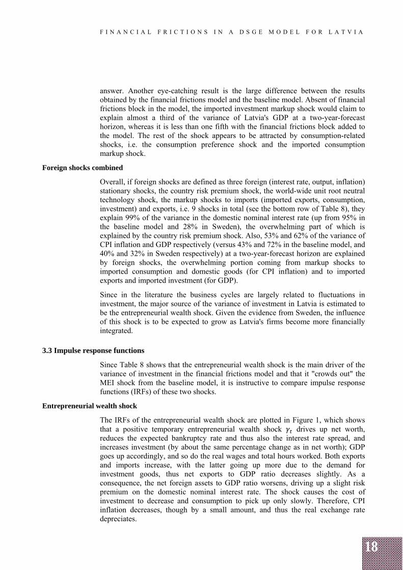
The IRFs of the entrepreneurial wealth shock are plotted in Figure 1, which shows that a positive temporary entrepreneurial wealth shock drives up net worth, reduces the expected bankruptcy rate and thus also the interest rate spread, and increases investment (by about the same percentage change as in net worth); GDP goes up accordingly, and so do the real wages and total hours worked. Both exports and imports increase, with the latter going up more due to the demand for investment goods, thus net exports to GDP ratio decreases slightly. As a consequence, the net foreign assets to GDP ratio worsens, driving up a slight risk premium on the domestic nominal interest rate. The shock causes the cost of investment to decrease and consumption to pick up only slowly. Therefore, CPI inflation decreases, though by a small amount, and thus the real exchange rate depreciates.
19
F I N A N C I A L F R I C T I O N S I N A D S G E M O D E L F O R L A T V I A
The response of net worth to this and other shocks is quite muted, i.e. its dynamics appear to die out in a few periods. This observation together with the autocorrelated measurement error of net worth suggest that the stock market price index might be a weak proxy for net worth in Latvia, and thus other potential measures, such as the house price index, could be investigated. Such an option is left for future research.
Figure 1 Impulse responses to entrepreneur wealth shock
Note: Units on the y-axis are either in terms of percentage deviation (% dev.) from the steady state, annualised basis points (ABP) or level deviation (Lev. dev.).
MEI shock
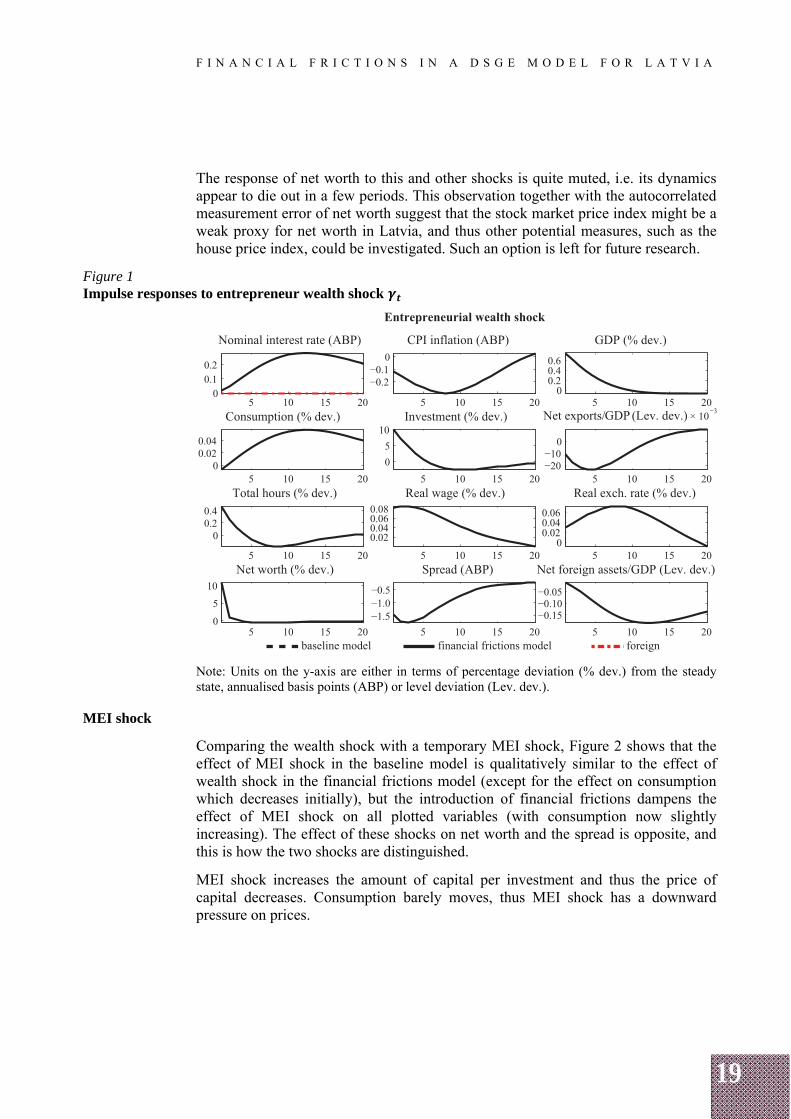
Comparing the wealth shock with a temporary MEI shock, Figure 2 shows that the effect of MEI shock in the baseline model is qualitatively similar to the effect of wealth shock in the financial frictions model (except for the effect on consumption which decreases initially), but the introduction of financial frictions dampens the effect of MEI shock on all plotted variables (with consumption now slightly increasing). The effect of these shocks on net worth and the spread is opposite, and this is how the two shocks are distinguished.
MEI shock increases the amount of capital per investment and thus the price of capital decreases. Consumption barely moves, thus MEI shock has a downward pressure on prices.
20
F I N A N C I A L F R I C T I O N S I N A D S G E M O D E L F O R L A T V I A
Figure 2 Impulse responses to marginal efficiency of investment shock
Note: Units on the y-axis are either in terms of percentage deviation (% dev.) from the steady state, annualised basis points (ABP) or level deviation (Lev. dev.).
Country risk premium shock
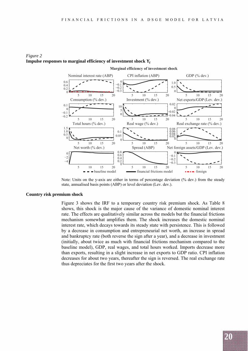
Figure 3 shows the IRF to a temporary country risk premium shock. As Table 8 shows, this shock is the major cause of the variance of domestic nominal interest rate. The effects are qualitatively similar across the models but the financial frictions mechanism somewhat amplifies them. The shock increases the domestic nominal interest rate, which decays towards its steady state with persistence. This is followed by a decrease in consumption and entrepreneurial net worth, an increase in spread and bankruptcy rate (both reverse the sign after a year), and a decrease in investment (initially, about twice as much with financial frictions mechanism compared to the baseline model), GDP, real wages, and total hours worked. Imports decrease more than exports, resulting in a slight increase in net exports to GDP ratio. CPI inflation decreases for about two years, thereafter the sign is reversed. The real exchange rate thus depreciates for the first two years after the shock.
21
F I N A N C I A L F R I C T I O N S I N A D S G E M O D E L F O R L A T V I A
Figure 3 Impulse responses to country risk premium shock
Note: Units on the y-axis are either in terms of percentage deviation (% dev.) from the steady state, annualised basis points (ABP) or level deviation (Lev. dev.).
Foreign nominal interest rate shock
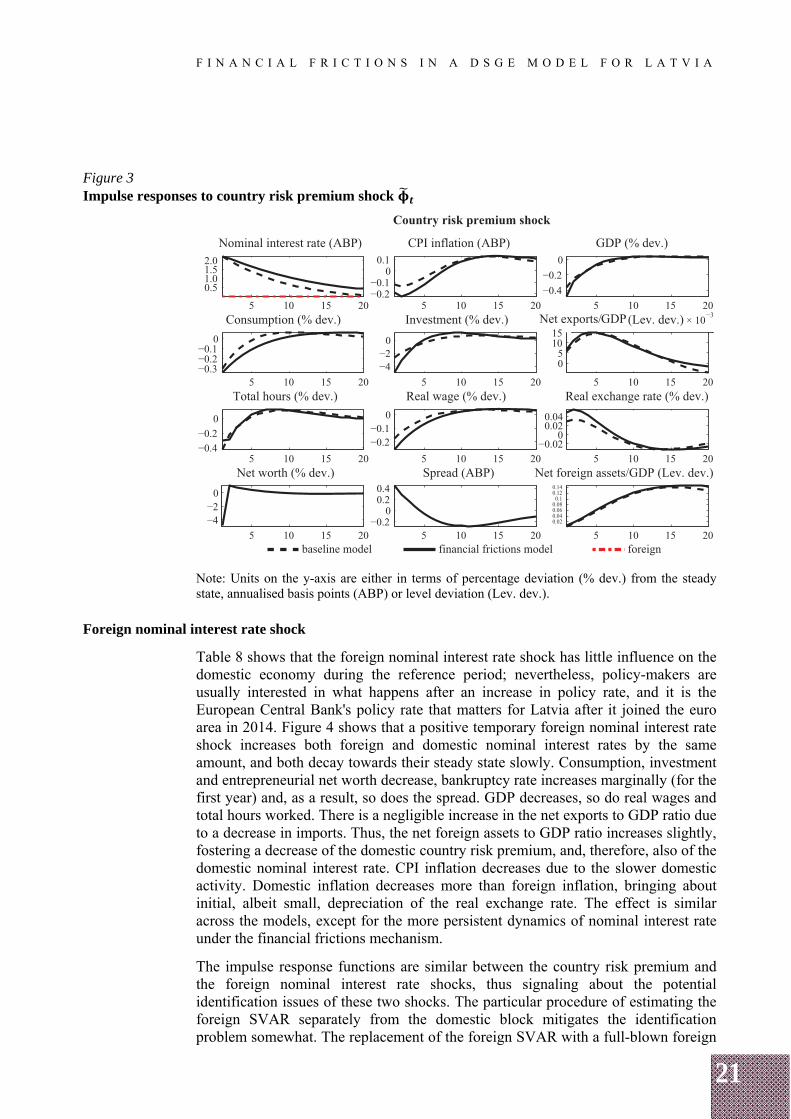
Table 8 shows that the foreign nominal interest rate shock has little influence on the domestic economy during the reference period; nevertheless, policy-makers are usually interested in what happens after an increase in policy rate, and it is the European Central Bank's policy rate that matters for Latvia after it joined the euro area in 2014. Figure 4 shows that a positive temporary foreign nominal interest rate shock increases both foreign and domestic nominal interest rates by the same amount, and both decay towards their steady state slowly. Consumption, investment and entrepreneurial net worth decrease, bankruptcy rate increases marginally (for the first year) and, as a result, so does the spread. GDP decreases, so do real wages and total hours worked. There is a negligible increase in the net exports to GDP ratio due to a decrease in imports. Thus, the net foreign assets to GDP ratio increases slightly, fostering a decrease of the domestic country risk premium, and, therefore, also of the domestic nominal interest rate. CPI inflation decreases due to the slower domestic activity. Domestic inflation decreases more than foreign inflation, bringing about initial, albeit small, depreciation of the real exchange rate. The effect is similar across the models, except for the more persistent dynamics of nominal interest rate under the financial frictions mechanism.
The impulse response functions are similar between the country risk premium and the foreign nominal interest rate shocks, thus signaling about the potential identification issues of these two shocks. The particular procedure of estimating the foreign SVAR separately from the domestic block mitigates the identification problem somewhat. The replacement of the foreign SVAR with a full-blown foreign

22
F I N A N C I A L F R I C T I O N S I N A D S G E M O D E L F O R L A T V I A
DSGE block could be a cure since it would identify the foreign monetary policy better but at the cost of model complexity.
The rest of IRFs are plotted in Appendix A.
Figure 4 Impulse responses to foreign nominal interest rate shock ∗,
Note: Units on the y-axis are either in terms of percentage deviation (% dev.) from the steady state, annualised basis points (ABP), or level deviation (Lev. dev.).
3.4 Smoothed shock values and historical decomposition
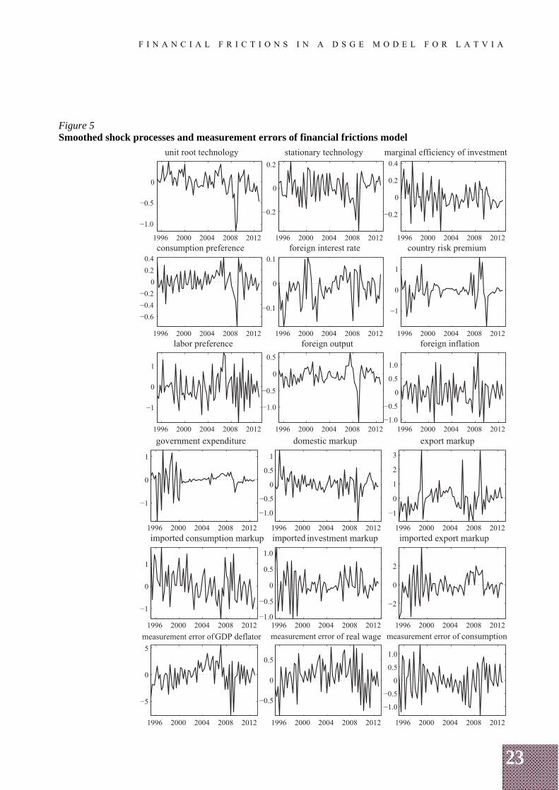
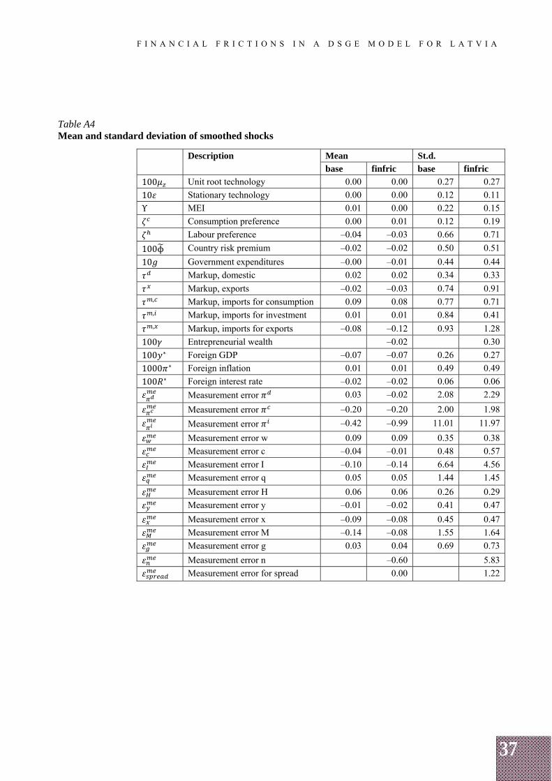
Figure 5 shows the smoothed shock values for the financial frictions model. The table summarising their means and standard deviations are relegated to Appendix A. These figures show that the means of shocks are at about zero. On the downside, the measurement errors of net worth, total hours worked and real wages appear to be autocorrelated.
23
F I N A N C I A L F R I C T I O N S I N A D S G E M O D E L F O R L A T V I A
Figure 5 Smoothed shock processes and measurement errors of financial frictions model

24
F I N A N C I A L F R I C T I O N S I N A D S G E M O D E L F O R L A T V I A
Figure 5 (continued) Smoothed shock processes and measurement errors of financial frictions model
Figures 6 to 12 show the historic shock decomposition of GDP, CPI inflation and interest rate spread.
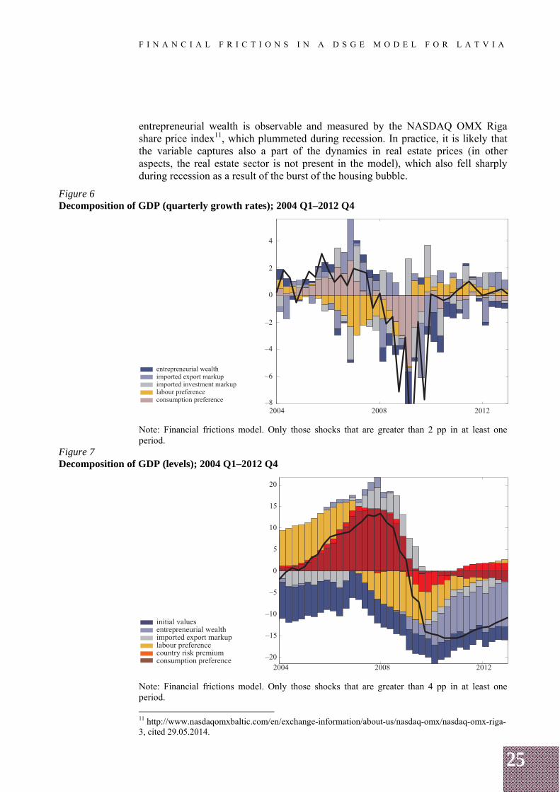
GDP Concentrating on the most sizable shocks, Figures 6 and 7 show that the model identifies the shock to household consumption preferences as the most important driving force of the 2004 boom. During the period from 2004 to 2007, the values of this shock were persistently above the sample average (see Figure 5), signifying that households were especially keen on spending for consumption goods during that period. The shock ceased during the second half of 2007, probably due to the rising costs of living and consequently decreasing consumer confidence (the latter is backed by the ECFIN consumer survey data). At that time, several other shocks became adverse, including stationary and unit-root neutral technology shocks, and the risk premium shock (see Figure 5). From 2008 up to 2011, a series of negative entrepreneurial wealth shocks is identified to have significantly affected the GDP growth (Figure 6). In fact, this shock became a major source determining the GDP level during the post-recession episode (see Figure 7). In the model, the dynamics of
25
F I N A N C I A L F R I C T I O N S I N A D S G E M O D E L F O R L A T V I A
entrepreneurial wealth is observable and measured by the NASDAQ OMX Riga share price index11, which plummeted during recession. In practice, it is likely that the variable captures also a part of the dynamics in real estate prices (in other aspects, the real estate sector is not present in the model), which also fell sharply during recession as a result of the burst of the housing bubble.
Figure 6 Decomposition of GDP (quarterly growth rates); 2004 Q1–2012 Q4
Note: Financial frictions model. Only those shocks that are greater than 2 pp in at least one period.
Figure 7 Decomposition of GDP (levels); 2004 Q1–2012 Q4
Note: Financial frictions model. Only those shocks that are greater than 4 pp in at least one period.
11 http://www.nasdaqomxbaltic.com/en/exchange-information/about-us/nasdaq-omx/nasdaq-omx-riga-3, cited 29.05.2014.
26
F I N A N C I A L F R I C T I O N S I N A D S G E M O D E L F O R L A T V I A
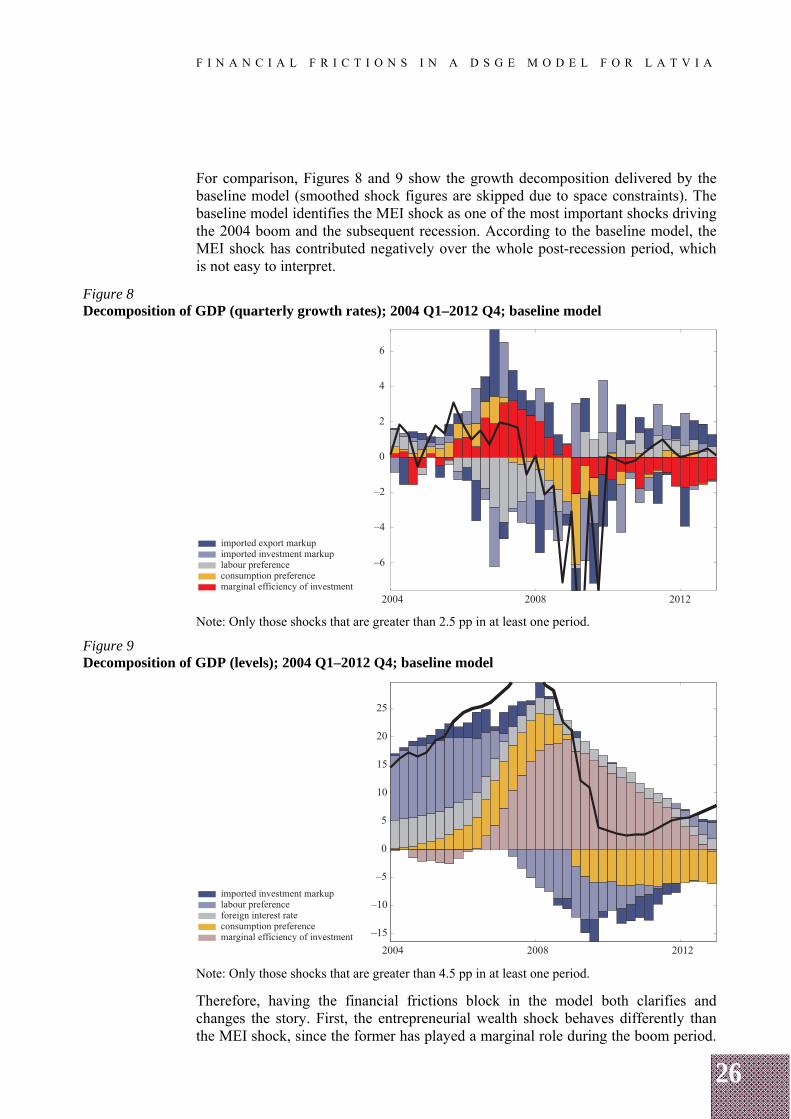
For comparison, Figures 8 and 9 show the growth decomposition delivered by the baseline model (smoothed shock figures are skipped due to space constraints). The baseline model identifies the MEI shock as one of the most important shocks driving the 2004 boom and the subsequent recession. According to the baseline model, the MEI shock has contributed negatively over the whole post-recession period, which is not easy to interpret.
Figure 8 Decomposition of GDP (quarterly growth rates); 2004 Q1–2012 Q4; baseline model
Note: Only those shocks that are greater than 2.5 pp in at least one period.
Figure 9 Decomposition of GDP (levels); 2004 Q1–2012 Q4; baseline model
Note: Only those shocks that are greater than 4.5 pp in at least one period.
Therefore, having the financial frictions block in the model both clarifies and changes the story. First, the entrepreneurial wealth shock behaves differently than the MEI shock, since the former has played a marginal role during the boom period.
27
F I N A N C I A L F R I C T I O N S I N A D S G E M O D E L F O R L A T V I A
Thus, consumption preferences are left as the single most important factor creating the 2004 boom. Second, the entrepreneurial wealth shock is a more easily understandable force that has deepened recession but ceased to be active during the post-recession episode. The ever-active MEI shock during the post-recession period, on the contrary, is harder to explicate in the baseline model.
CPI inflation
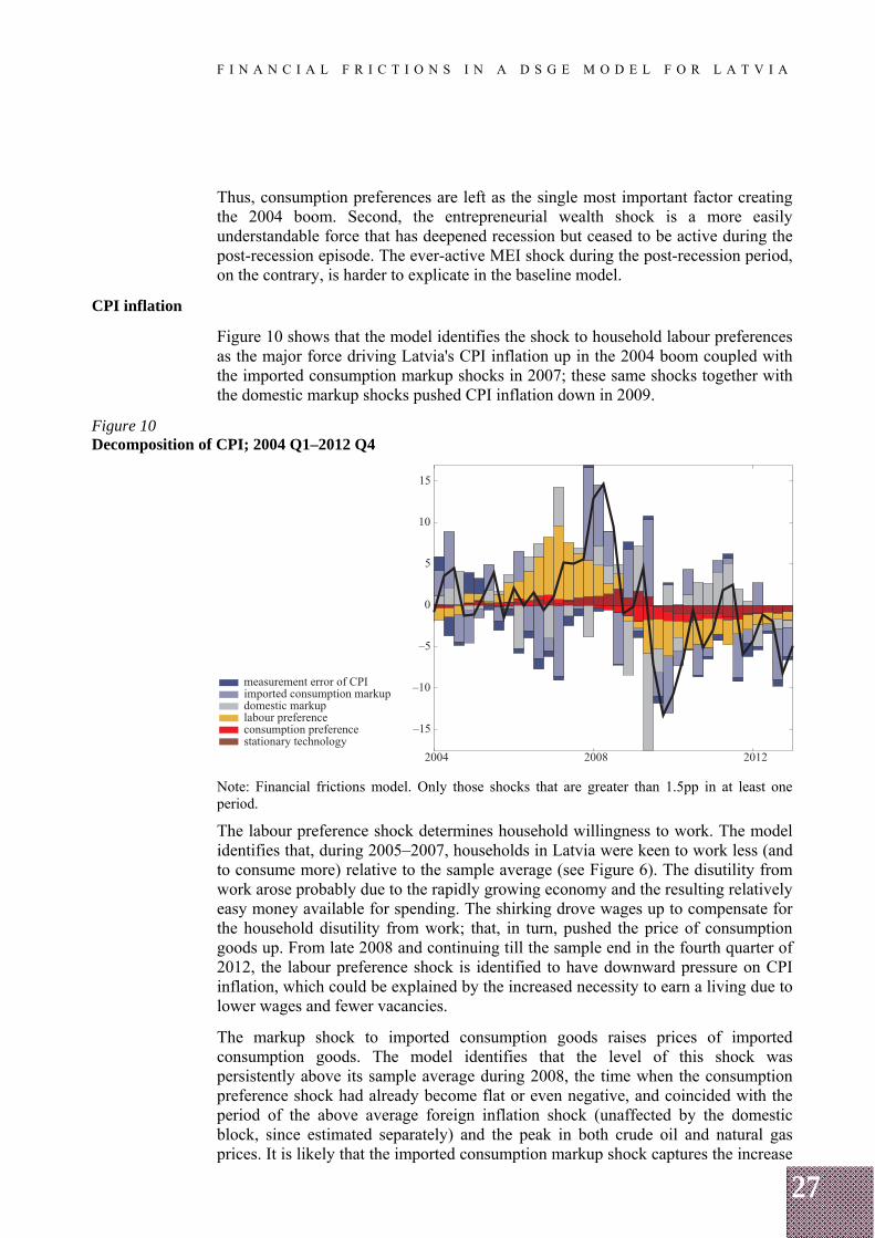
Figure 10 shows that the model identifies the shock to household labour preferences as the major force driving Latvia's CPI inflation up in the 2004 boom coupled with the imported consumption markup shocks in 2007; these same shocks together with the domestic markup shocks pushed CPI inflation down in 2009.
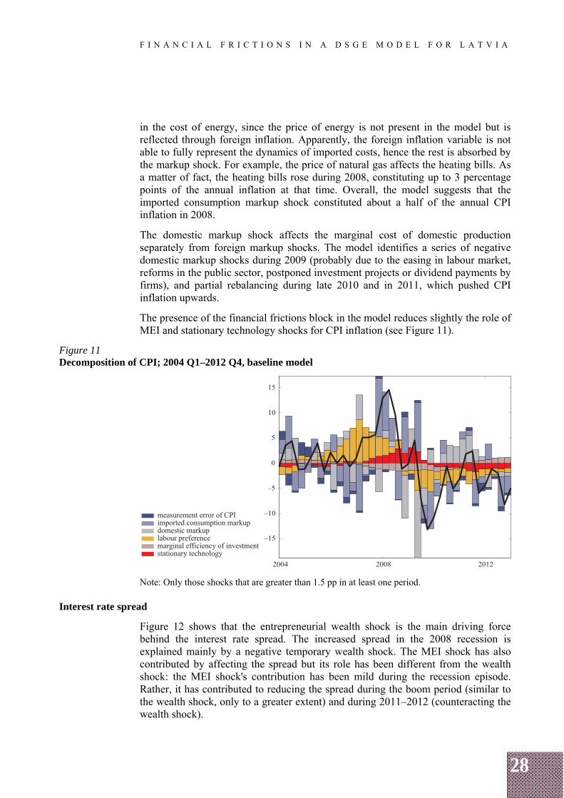
Figure 10 Decomposition of CPI; 2004 Q1–2012 Q4
Note: Financial frictions model. Only those shocks that are greater than 1.5pp in at least one period.
The labour preference shock determines household willingness to work. The model identifies that, during 2005–2007, households in Latvia were keen to work less (and to consume more) relative to the sample average (see Figure 6). The disutility from work arose probably due to the rapidly growing economy and the resulting relatively easy money available for spending. The shirking drove wages up to compensate for the household disutility from work; that, in turn, pushed the price of consumption goods up. From late 2008 and continuing till the sample end in the fourth quarter of 2012, the labour preference shock is identified to have downward pressure on CPI inflation, which could be explained by the increased necessity to earn a living due to lower wages and fewer vacancies.
The markup shock to imported consumption goods raises prices of imported consumption goods. The model identifies that the level of this shock was persistently above its sample average during 2008, the time when the consumption preference shock had already become flat or even negative, and coincided with the period of the above average foreign inflation shock (unaffected by the domestic block, since estimated separately) and the peak in both crude oil and natural gas prices. It is likely that the imported consumption markup shock captures the increase
28
F I N A N C I A L F R I C T I O N S I N A D S G E M O D E L F O R L A T V I A
in the cost of energy, since the price of energy is not present in the model but is reflected through foreign inflation. Apparently, the foreign inflation variable is not able to fully represent the dynamics of imported costs, hence the rest is absorbed by the markup shock. For example, the price of natural gas affects the heating bills. As a matter of fact, the heating bills rose during 2008, constituting up to 3 percentage points of the annual inflation at that time. Overall, the model suggests that the imported consumption markup shock constituted about a half of the annual CPI inflation in 2008.
The domestic markup shock affects the marginal cost of domestic production separately from foreign markup shocks. The model identifies a series of negative domestic markup shocks during 2009 (probably due to the easing in labour market, reforms in the public sector, postponed investment projects or dividend payments by firms), and partial rebalancing during late 2010 and in 2011, which pushed CPI inflation upwards.
The presence of the financial frictions block in the model reduces slightly the role of MEI and stationary technology shocks for CPI inflation (see Figure 11).
Figure 11 Decomposition of CPI; 2004 Q1–2012 Q4, baseline model
Note: Only those shocks that are greater than 1.5 pp in at least one period.
Interest rate spread
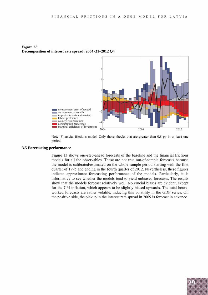
Figure 12 shows that the entrepreneurial wealth shock is the main driving force behind the interest rate spread. The increased spread in the 2008 recession is explained mainly by a negative temporary wealth shock. The MEI shock has also contributed by affecting the spread but its role has been different from the wealth shock: the MEI shock's contribution has been mild during the recession episode. Rather, it has contributed to reducing the spread during the boom period (similar to the wealth shock, only to a greater extent) and during 2011–2012 (counteracting the wealth shock).
29
F I N A N C I A L F R I C T I O N S I N A D S G E M O D E L F O R L A T V I A
Figure 12 Decomposition of interest rate spread; 2004 Q1–2012 Q4
Note: Financial frictions model. Only those shocks that are greater than 0.8 pp in at least one period.
3.5 Forecasting performance
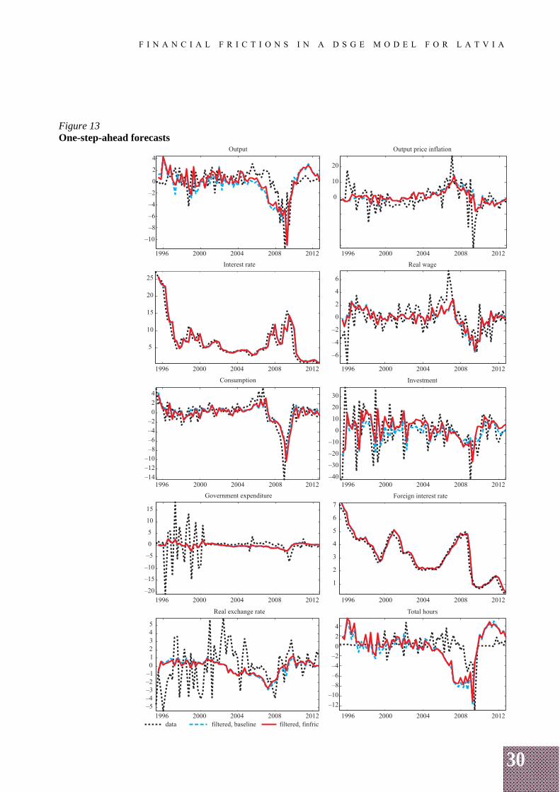
Figure 13 shows one-step-ahead forecasts of the baseline and the financial frictions models for all the observables. These are not true out-of-sample forecasts because the model is calibrated/estimated on the whole sample period starting with the first quarter of 1995 and ending in the fourth quarter of 2012. Nevertheless, these figures indicate approximate forecasting performance of the models. Particularly, it is informative to see whether the models tend to yield unbiased forecasts. The results show that the models forecast relatively well. No crucial biases are evident, except for the CPI inflation, which appears to be slightly biased upwards. The total-hours-worked forecasts are rather volatile, inducing this volatility in the GDP series. On the positive side, the pickup in the interest rate spread in 2009 is forecast in advance.
30
F I N A N C I A L F R I C T I O N S I N A D S G E M O D E L F O R L A T V I A
Figure 13 One-step-ahead forecasts
31
F I N A N C I A L F R I C T I O N S I N A D S G E M O D E L F O R L A T V I A
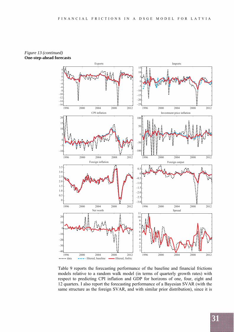
Figure 13 (continued) One-step-ahead forecasts
Table 9 reports the forecasting performance of the baseline and financial frictions models relative to a random walk model (in terms of quarterly growth rates) with respect to predicting CPI inflation and GDP for horizons of one, four, eight and 12 quarters. I also report the forecasting performance of a Bayesian SVAR (with the same structure as the foreign SVAR, and with similar prior distribution), since it is
32
F I N A N C I A L F R I C T I O N S I N A D S G E M O D E L F O R L A T V I A
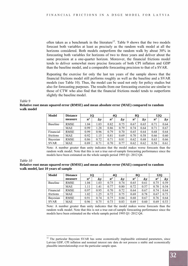
often taken as a benchmark in the literature12. Table 9 shows that the two models forecast both variables at least as precisely as the random walk model at all the horizons considered. Both models outperform the random walk by about 30% in forecasting both variables for horizons of two to three years and deliver about the same precision at a one-quarter horizon. Moreover, the financial frictions model tends to deliver somewhat more precise forecasts of both CPI inflation and GDP than the baseline model, and a comparable forecasting precision to that of a SVAR.
Repeating the exercise for only the last ten years of the sample shows that the financial frictions model still performs roughly as well as the baseline and a SVAR models (see Table 10). Thus, the model can be used not only for policy studies but also for forecasting purposes. The results from our forecasting exercise are similar to those of CTW who also find that the financial frictions model tends to outperform slightly the baseline model.
Table 9 Relative root mean squared error (RMSE) and mean absolute error (MAE) compared to random walk model
Model
Distance measure
1Q 4Q 8Q 12Q
Baseline RMSE 1.04 1.03 0.82 0.75 0.67 0.65 0.71 0.64 MAE 0.99 1.28 0.86 0.79 0.74 0.64 0.71 0.67
Financial frictions
RMSE 0.99 0.96 0.79 0.70 0.65 0.64 0.68 0.64 MAE 0.92 1.15 0.81 0.69 0.70 0.58 0.66 0.60
Bayesian SVAR
RMSE 0.86 0.72 0.71 0.81 0.62 0.68 0.63 0.66 MAE 0.89 0.71 0.70 0.77 0.62 0.62 0.58 0.61
Note: A number greater than unity indicates that the model makes worse forecasts than the random walk model. Note that this is not a true out-of-sample forecasting performance since the models have been estimated on the whole sample period 1995 Q1–2012 Q4.
Table 10 Relative root mean squared error (RMSE) and mean absolute error (MAE) compared to random walk model, last 10 years of sample
Model Distance measure
1Q 4Q 8Q 12Q
Baseline RMSE 1.04 1.03 0.75 0.74 0.65 0.61 0.75 0.59 MAE 1.11 1.41 0.77 0.80 0.72 0.57 0.70 0.54
Financial frictions
RMSE 0.97 0.95 0.70 0.72 0.64 0.67 0.74 0.64 MAE 1.02 1.25 0.72 0.75 0.69 0.78 0.67 0.73
Bayesian SVAR
RMSE 0.91 0.74 0.75 0.84 0.68 0.67 0.76 0.64 MAE 0.96 0.75 0.73 0.83 0.69 0.60 0.69 0.53
Note: A number greater than unity indicates that the model makes worse forecasts than the random walk model. Note that this is not a true out-of-sample forecasting performance since the models have been estimated on the whole sample period 1995 Q1–2012 Q4.
12 The particular Bayesian SVAR has some economically implausible estimated parameters, since Latvian GDP, CPI inflation and nominal interest rate data do not possess a stable and economically plausible interrelationship over the particular sample span.
33
F I N A N C I A L F R I C T I O N S I N A D S G E M O D E L F O R L A T V I A
4. CONCLUSIONS
This paper builds a DSGE model for Latvia that would be suitable to replace the traditional macroeconometric model currently employed as the main macroeconomic model at Latvijas Banka. For that purpose, the financial frictions model of Christiano, Trabandt and Walentin (2011) is adapted for Latvia's data. The monetary policy is altered to become a nominal interest rate peg to the foreign interest rate. The paper studies model fit, impulse response functions, conditional forecast variance decomposition, shock historic decomposition and forecasting performance and compares the outcome to that of a model without financial accelerator block (the baseline model) as well as to the findings by CTW.
The main findings are as follows. The adding of financial frictions block provides a more appealing interpretation for the drivers of economic activity, and allows to reinterpret their role. Financial frictions played an important part in Latvia's 2008 recession. The financial frictions model beats both the baseline model and the random walk model in forecasting CPI inflation and GDP, and performs roughly the same as a Bayesian SVAR.
Overall, the results suggest that the financial frictions model is suitable for both policy analysis and forecasting exercises and is an improvement over the model without the financial frictions block.
34
F I N A N C I A L F R I C T I O N S I N A D S G E M O D E L F O R L A T V I A
APPENDICES
Appendix A
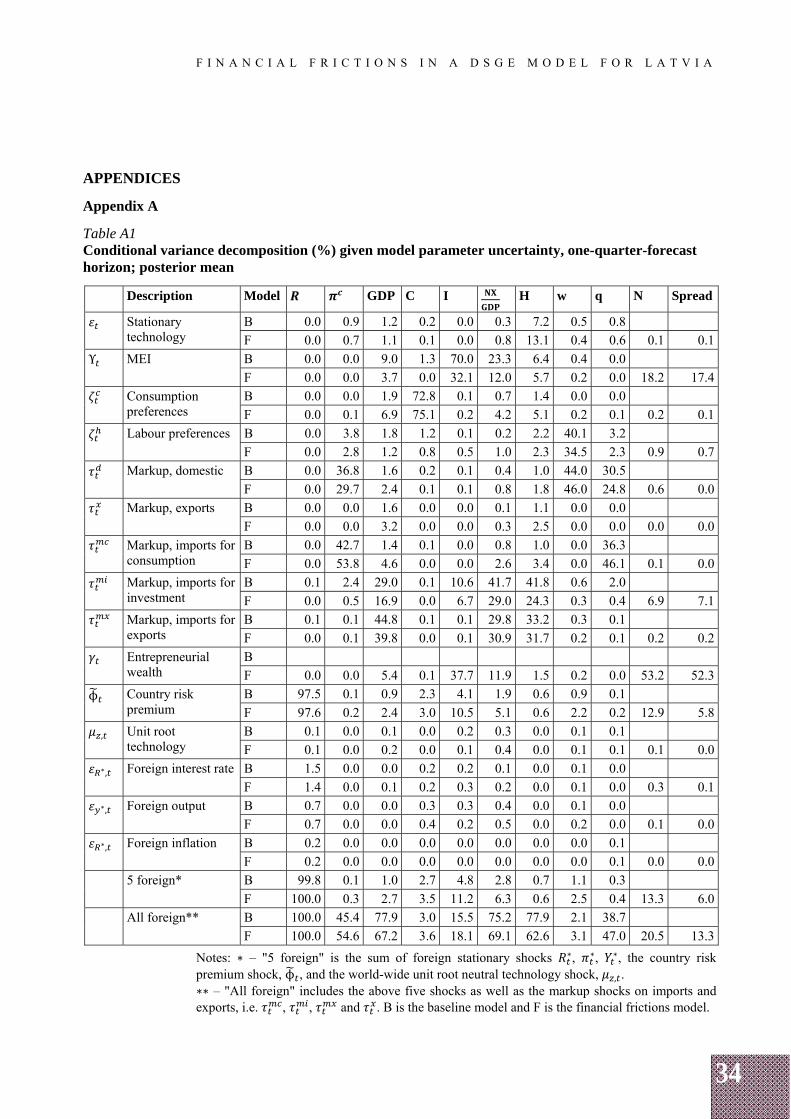
Table A1 Conditional variance decomposition (%) given model parameter uncertainty, one-quarter-forecast horizon; posterior mean
Description Model GDP C I H w q N Spread
Stationary technology
B 0.0 0.9 1.2 0.2 0.0 0.3 7.2 0.5 0.8
F 0.0 0.7 1.1 0.1 0.0 0.8 13.1 0.4 0.6 0.1 0.1
Υ MEI B 0.0 0.0 9.0 1.3 70.0 23.3 6.4 0.4 0.0
F 0.0 0.0 3.7 0.0 32.1 12.0 5.7 0.2 0.0 18.2 17.4
Consumption preferences
B 0.0 0.0 1.9 72.8 0.1 0.7 1.4 0.0 0.0
F 0.0 0.1 6.9 75.1 0.2 4.2 5.1 0.2 0.1 0.2 0.1
Labour preferences B 0.0 3.8 1.8 1.2 0.1 0.2 2.2 40.1 3.2
F 0.0 2.8 1.2 0.8 0.5 1.0 2.3 34.5 2.3 0.9 0.7
Markup, domestic B 0.0 36.8 1.6 0.2 0.1 0.4 1.0 44.0 30.5
F 0.0 29.7 2.4 0.1 0.1 0.8 1.8 46.0 24.8 0.6 0.0
Markup, exports B 0.0 0.0 1.6 0.0 0.0 0.1 1.1 0.0 0.0
F 0.0 0.0 3.2 0.0 0.0 0.3 2.5 0.0 0.0 0.0 0.0
Markup, imports for consumption
B 0.0 42.7 1.4 0.1 0.0 0.8 1.0 0.0 36.3
F 0.0 53.8 4.6 0.0 0.0 2.6 3.4 0.0 46.1 0.1 0.0
Markup, imports for investment
B 0.1 2.4 29.0 0.1 10.6 41.7 41.8 0.6 2.0
F 0.0 0.5 16.9 0.0 6.7 29.0 24.3 0.3 0.4 6.9 7.1
Markup, imports for exports
B 0.1 0.1 44.8 0.1 0.1 29.8 33.2 0.3 0.1
F 0.0 0.1 39.8 0.0 0.1 30.9 31.7 0.2 0.1 0.2 0.2
Entrepreneurial wealth
B
F 0.0 0.0 5.4 0.1 37.7 11.9 1.5 0.2 0.0 53.2 52.3
ϕ Country risk premium
B 97.5 0.1 0.9 2.3 4.1 1.9 0.6 0.9 0.1
F 97.6 0.2 2.4 3.0 10.5 5.1 0.6 2.2 0.2 12.9 5.8
, Unit root technology
B 0.1 0.0 0.1 0.0 0.2 0.3 0.0 0.1 0.1
F 0.1 0.0 0.2 0.0 0.1 0.4 0.0 0.1 0.1 0.1 0.0∗, Foreign interest rate B 1.5 0.0 0.0 0.2 0.2 0.1 0.0 0.1 0.0
F 1.4 0.0 0.1 0.2 0.3 0.2 0.0 0.1 0.0 0.3 0.1∗, Foreign output B 0.7 0.0 0.0 0.3 0.3 0.4 0.0 0.1 0.0
F 0.7 0.0 0.0 0.4 0.2 0.5 0.0 0.2 0.0 0.1 0.0∗, Foreign inflation B 0.2 0.0 0.0 0.0 0.0 0.0 0.0 0.0 0.1
F 0.2 0.0 0.0 0.0 0.0 0.0 0.0 0.0 0.1 0.0 0.0
5 foreign* B 99.8 0.1 1.0 2.7 4.8 2.8 0.7 1.1 0.3
F 100.0 0.3 2.7 3.5 11.2 6.3 0.6 2.5 0.4 13.3 6.0
All foreign** B 100.0 45.4 77.9 3.0 15.5 75.2 77.9 2.1 38.7
F 100.0 54.6 67.2 3.6 18.1 69.1 62.6 3.1 47.0 20.5 13.3
Notes: ∗ – "5 foreign" is the sum of foreign stationary shocks ∗, ∗, ∗, the country risk premium shock, ϕ , and the world-wide unit root neutral technology shock, , . ∗∗ – "All foreign" includes the above five shocks as well as the markup shocks on imports and exports, i.e. , , and . B is the baseline model and F is the financial frictions model.
35
F I N A N C I A L F R I C T I O N S I N A D S G E M O D E L F O R L A T V I A
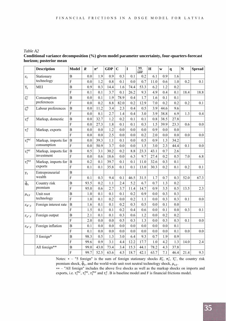
Table A2 Conditional variance decomposition (%) given model parameter uncertainty, four-quarters-forecast horizon; posterior mean
Description Model GDP C I H w q N Spread
Stationary technology
B 0.0 1.9 0.9 0.3 0.1 0.2 6.1 0.9 1.6
F 0.0 1.2 0.8 0.1 0.0 0.7 11.0 0.6 1.0 0.2 0.1
Υ MEI B 0.9 0.3 14.4 1.6 74.4 53.3 6.2 1.2 0.2
F 0.1 0.1 3.7 0.1 26.2 9.3 4.9 0.4 0.1 18.4 18.8
Consumption preferences
B 0.0 0.1 1.9 78.9 0.4 1.7 1.6 0.1 0.1
F 0.0 0.2 8.8 82.0 0.2 12.9 7.0 0.2 0.2 0.2 0.1
Labour preferences B 0.0 11.2 3.4 2.3 0.4 0.5 3.9 44.6 9.6
F 0.0 8.1 2.7 1.4 0.4 3.0 3.9 38.8 6.9 1.3 0.4
Markup, domestic B 0.0 32.7 1.2 0.2 0.1 0.1 0.8 38.5 27.8
F 0.0 27.3 1.8 0.1 0.1 0.3 1.5 39.9 23.3 0.6 0.0
Markup, exports B 0.0 0.0 1.2 0.0 0.0 0.0 0.9 0.0 0.0
F 0.0 0.0 2.5 0.0 0.0 0.2 2.0 0.0 0.0 0.0 0.0
Markup, imports for consumption
B 0.0 39.3 1.1 0.1 0.0 0.5 0.9 1.3 34.2
F 0.0 50.9 3.7 0.0 0.0 1.5 3.0 2.3 44.4 0.1 0.0
Markup, imports for investment
B 0.5 3.1 30.2 0.2 8.8 23.3 43.1 0.7 2.6
F 0.0 0.6 18.6 0.0 6.3 9.7 27.4 0.2 0.5 7.0 6.8
Markup, imports for exports
B 0.2 0.1 39.7 0.1 0.1 11.0 32.6 0.3 0.1
F 0.1 0.1 35.8 0.1 0.1 13.0 30.3 0.2 0.1 0.2 0.1
Entrepreneurial wealth
B
F 0.1 0.3 9.4 0.1 46.5 31.5 1.7 0.7 0.3 52.0 67.3
ϕ Country risk premium
B 93.5 0.2 1.1 2.4 5.2 6.7 0.7 1.3 0.2
F 95.0 0.6 2.7 3.7 11.4 14.7 0.9 3.5 0.5 13.5 2.3
, Unit root technology
B 1.0 0.1 0.1 0.1 0.2 0.9 0.0 0.3 0.3
F 1.0 0.1 0.2 0.0 0.2 1.1 0.0 0.3 0.3 0.1 0.0∗, Foreign interest rate B 1.6 0.1 0.1 0.2 0.3 0.5 0.0 0.1 0.0
F 1.5 0.1 0.1 0.2 0.4 0.6 0.0 0.1 0.0 0.3 0.1∗, Foreign output B 2.1 0.1 0.1 0.3 0.6 1.2 0.0 0.2 0.2
F 2.0 0.0 0.0 0.5 0.3 1.3 0.0 0.3 0.3 0.1 0.0∗, Foreign inflation B 0.1 0.0 0.0 0.0 0.0 0.0 0.0 0.0 0.1
F 0.1 0.0 0.0 0.0 0.0 0.0 0.0 0.0 0.1 0.0 0.0
5 foreign* B 98.3 0.5 1.3 3.0 6.4 9.3 0.7 1.9 0.9
F 99.6 0.9 3.1 4.4 12.2 17.7 1.0 4.2 1.3 14.0 2.4
All foreign** B 99.0 43.0 73.4 3.4 15.3 44.1 78.2 4.3 37.8
F 99.7 52.5 63.6 4.5 18.7 42.1 63.7 7.1 46.4 21.4 9.3
Notes: ∗ – "5 foreign" is the sum of foreign stationary shocks ∗, ∗, ∗, the country risk premium shock, ϕ , and the world-wide unit root neutral technology shock, , . ∗∗ – "All foreign" includes the above five shocks as well as the markup shocks on imports and exports, i.e. , , and . B is baseline model and F is financial frictions model.
36
F I N A N C I A L F R I C T I O N S I N A D S G E M O D E L F O R L A T V I A
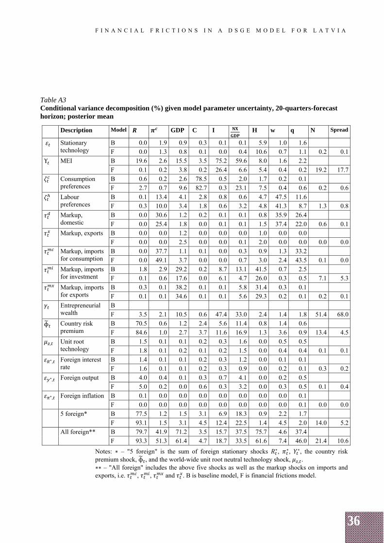
Table A3 Conditional variance decomposition (%) given model parameter uncertainty, 20-quarters-forecast horizon; posterior mean
Description Model GDP C I H w q N Spread
Stationary technology
B 0.0 1.9 0.9 0.3 0.1 0.1 5.9 1.0 1.6
F 0.0 1.3 0.8 0.1 0.0 0.4 10.6 0.7 1.1 0.2 0.1
Υ MEI B 19.6 2.6 15.5 3.5 75.2 59.6 8.0 1.6 2.2
F 0.1 0.2 3.8 0.2 26.4 6.6 5.4 0.4 0.2 19.2 17.7
Consumption preferences
B 0.6 0.2 2.6 78.5 0.5 2.0 1.7 0.2 0.1
F 2.7 0.7 9.6 82.7 0.3 23.1 7.5 0.4 0.6 0.2 0.6
Labour preferences
B 0.1 13.4 4.1 2.8 0.8 0.6 4.7 47.5 11.6
F 0.3 10.0 3.4 1.8 0.6 3.2 4.8 41.3 8.7 1.3 0.8
Markup, domestic
B 0.0 30.6 1.2 0.2 0.1 0.1 0.8 35.9 26.4
F 0.0 25.4 1.8 0.0 0.1 0.1 1.5 37.4 22.0 0.6 0.1
Markup, exports B 0.0 0.0 1.2 0.0 0.0 0.0 1.0 0.0 0.0
F 0.0 0.0 2.5 0.0 0.0 0.1 2.0 0.0 0.0 0.0 0.0
Markup, imports for consumption
B 0.0 37.7 1.1 0.1 0.0 0.3 0.9 1.3 33.2
F 0.0 49.1 3.7 0.0 0.0 0.7 3.0 2.4 43.5 0.1 0.0
Markup, imports for investment
B 1.8 2.9 29.2 0.2 8.7 13.1 41.5 0.7 2.5
F 0.1 0.6 17.6 0.0 6.1 4.7 26.0 0.3 0.5 7.1 5.3
Markup, imports for exports
B 0.3 0.1 38.2 0.1 0.1 5.8 31.4 0.3 0.1
F 0.1 0.1 34.6 0.1 0.1 5.6 29.3 0.2 0.1 0.2 0.1
Entrepreneurial wealth
B
F 3.5 2.1 10.5 0.6 47.4 33.0 2.4 1.4 1.8 51.4 68.0
ϕ Country risk premium
B 70.5 0.6 1.2 2.4 5.6 11.4 0.8 1.4 0.6
F 84.6 1.0 2.7 3.7 11.6 16.9 1.3 3.6 0.9 13.4 4.5
, Unit root technology
B 1.5 0.1 0.1 0.2 0.3 1.6 0.0 0.5 0.5
F 1.8 0.1 0.2 0.1 0.2 1.5 0.0 0.4 0.4 0.1 0.1∗, Foreign interest
rate B 1.4 0.1 0.1 0.2 0.3 1.2 0.0 0.1 0.1
F 1.6 0.1 0.1 0.2 0.3 0.9 0.0 0.2 0.1 0.3 0.2∗, Foreign output B 4.0 0.4 0.1 0.3 0.7 4.1 0.0 0.2 0.5
F 5.0 0.2 0.0 0.6 0.3 3.2 0.0 0.3 0.5 0.1 0.4∗, Foreign inflation B 0.1 0.0 0.0 0.0 0.0 0.0 0.0 0.0 0.1
F 0.0 0.0 0.0 0.0 0.0 0.0 0.0 0.0 0.1 0.0 0.0
5 foreign* B 77.5 1.2 1.5 3.1 6.9 18.3 0.9 2.2 1.7
F 93.1 1.5 3.1 4.5 12.4 22.5 1.4 4.5 2.0 14.0 5.2
All foreign** B 79.7 41.9 71.2 3.5 15.7 37.5 75.7 4.6 37.4
F 93.3 51.3 61.4 4.7 18.7 33.5 61.6 7.4 46.0 21.4 10.6
Notes: ∗ – "5 foreign" is the sum of foreign stationary shocks ∗, ∗, ∗, the country risk premium shock, ϕ , and the world-wide unit root neutral technology shock, , . ∗∗ – "All foreign" includes the above five shocks as well as the markup shocks on imports and exports, i.e. , , and . B is baseline model, F is financial frictions model.
37
F I N A N C I A L F R I C T I O N S I N A D S G E M O D E L F O R L A T V I A
Table A4 Mean and standard deviation of smoothed shocks
Description
Mean St.d.
base finfric base finfric
100 Unit root technology 0.00 0.00 0.27 0.27
10 Stationary technology 0.00 0.00 0.12 0.11
Υ MEI 0.01 0.00 0.22 0.15
Consumption preference 0.00 0.01 0.12 0.19
Labour preference –0.04 –0.03 0.66 0.71
100ϕ Country risk premium –0.02 –0.02 0.50 0.51
10 Government expenditures –0.00 –0.01 0.44 0.44
Markup, domestic 0.02 0.02 0.34 0.33
Markup, exports –0.02 –0.03 0.74 0.91 , Markup, imports for consumption 0.09 0.08 0.77 0.71 , Markup, imports for investment 0.01 0.01 0.84 0.41 , Markup, imports for exports –0.08 –0.12 0.93 1.28
100 Entrepreneurial wealth –0.02 0.30
100 ∗ Foreign GDP –0.07 –0.07 0.26 0.27
1000 ∗ Foreign inflation 0.01 0.01 0.49 0.49
100 ∗ Foreign interest rate –0.02 –0.02 0.06 0.06
Measurement error 0.03 –0.02 2.08 2.29
Measurement error –0.20 –0.20 2.00 1.98
Measurement error –0.42 –0.99 11.01 11.97
Measurement error w 0.09 0.09 0.35 0.38
Measurement error c –0.04 –0.01 0.48 0.57
Measurement error I –0.10 –0.14 6.64 4.56
Measurement error q 0.05 0.05 1.44 1.45
Measurement error H 0.06 0.06 0.26 0.29
Measurement error y –0.01 –0.02 0.41 0.47
Measurement error x –0.09 –0.08 0.45 0.47
Measurement error M –0.14 –0.08 1.55 1.64
Measurement error g 0.03 0.04 0.69 0.73
Measurement error n –0.60 5.83
Measurement error for spread 0.00 1.22
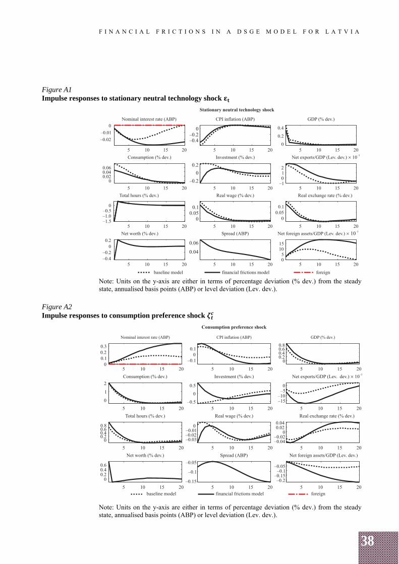
38
F I N A N C I A L F R I C T I O N S I N A D S G E M O D E L F O R L A T V I A
Figure A1 Impulse responses to stationary neutral technology shock
Note: Units on the y-axis are either in terms of percentage deviation (% dev.) from the steady state, annualised basis points (ABP) or level deviation (Lev. dev.).
Figure A2 Impulse responses to consumption preference shock
Note: Units on the y-axis are either in terms of percentage deviation (% dev.) from the steady state, annualised basis points (ABP) or level deviation (Lev. dev.).
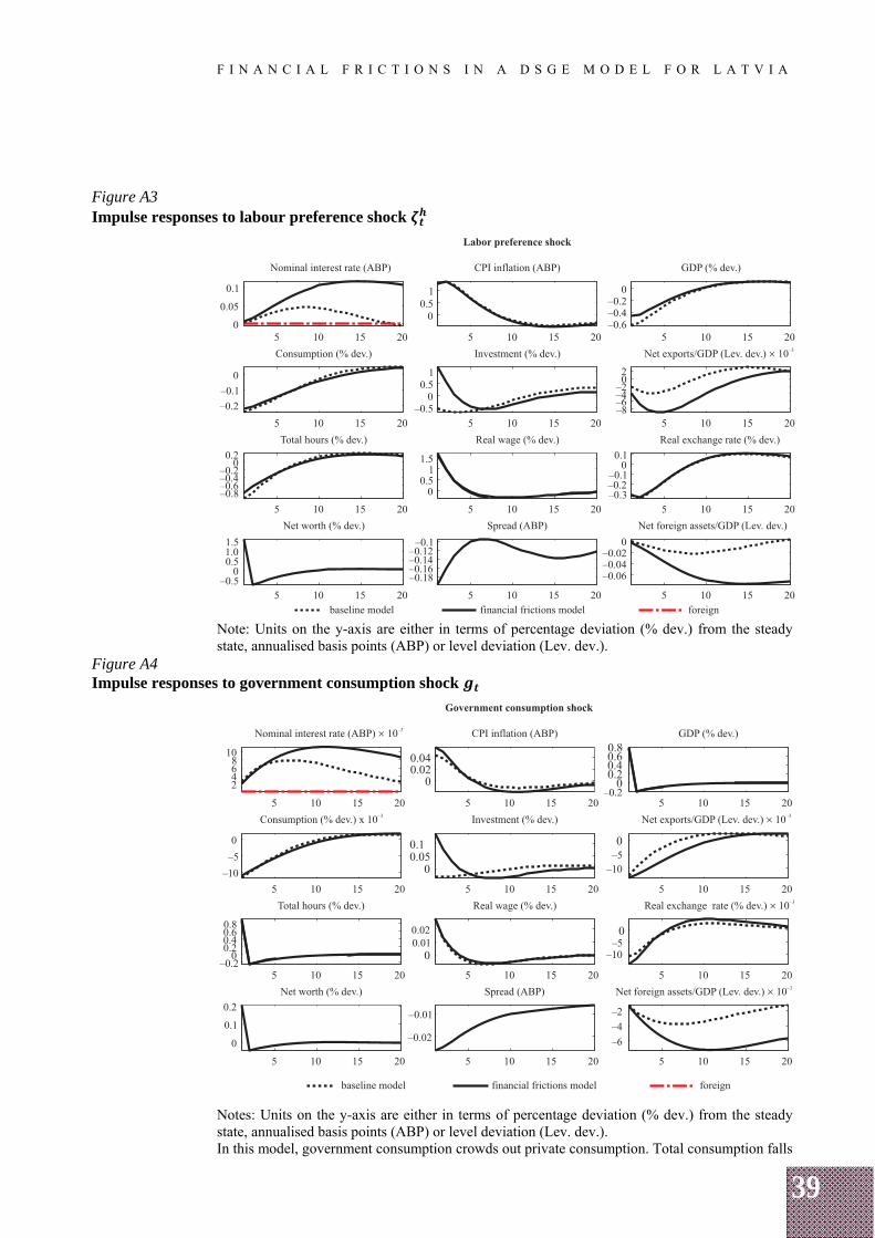
39
F I N A N C I A L F R I C T I O N S I N A D S G E M O D E L F O R L A T V I A
Figure A3 Impulse responses to labour preference shock
Note: Units on the y-axis are either in terms of percentage deviation (% dev.) from the steady state, annualised basis points (ABP) or level deviation (Lev. dev.).
Figure A4 Impulse responses to government consumption shock
Notes: Units on the y-axis are either in terms of percentage deviation (% dev.) from the steady state, annualised basis points (ABP) or level deviation (Lev. dev.). In this model, government consumption crowds out private consumption. Total consumption falls
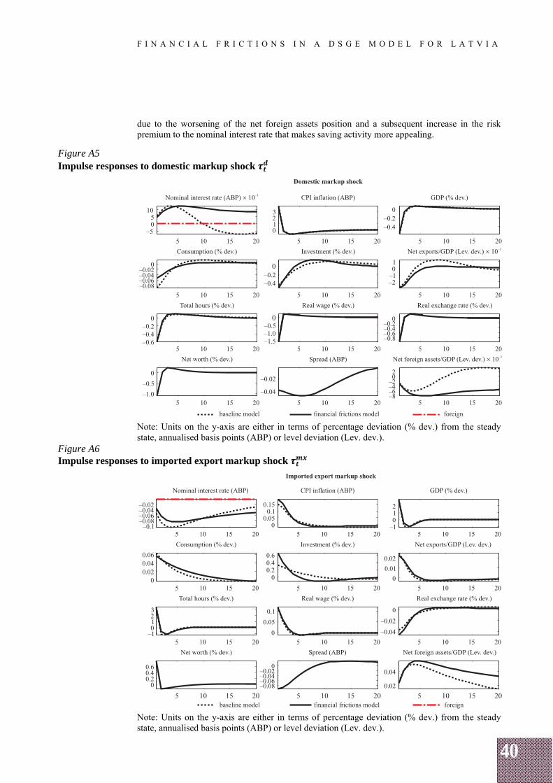
40
F I N A N C I A L F R I C T I O N S I N A D S G E M O D E L F O R L A T V I A
due to the worsening of the net foreign assets position and a subsequent increase in the risk premium to the nominal interest rate that makes saving activity more appealing.
Figure A5 Impulse responses to domestic markup shock
Note: Units on the y-axis are either in terms of percentage deviation (% dev.) from the steady state, annualised basis points (ABP) or level deviation (Lev. dev.).
Figure A6 Impulse responses to imported export markup shock
Note: Units on the y-axis are either in terms of percentage deviation (% dev.) from the steady state, annualised basis points (ABP) or level deviation (Lev. dev.).
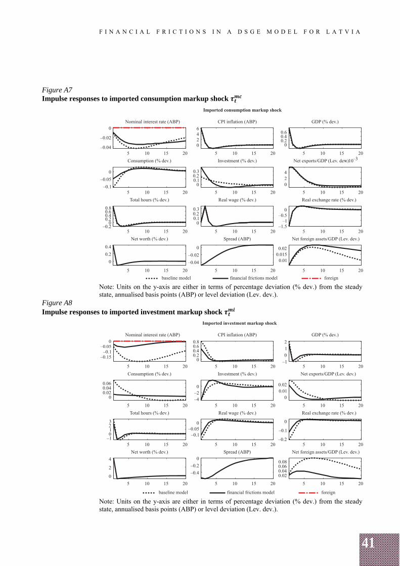
41
F I N A N C I A L F R I C T I O N S I N A D S G E M O D E L F O R L A T V I A
Figure A7 Impulse responses to imported consumption markup shock
Note: Units on the y-axis are either in terms of percentage deviation (% dev.) from the steady state, annualised basis points (ABP) or level deviation (Lev. dev.).
Figure A8 Impulse responses to imported investment markup shock
Note: Units on the y-axis are either in terms of percentage deviation (% dev.) from the steady state, annualised basis points (ABP) or level deviation (Lev. dev.).
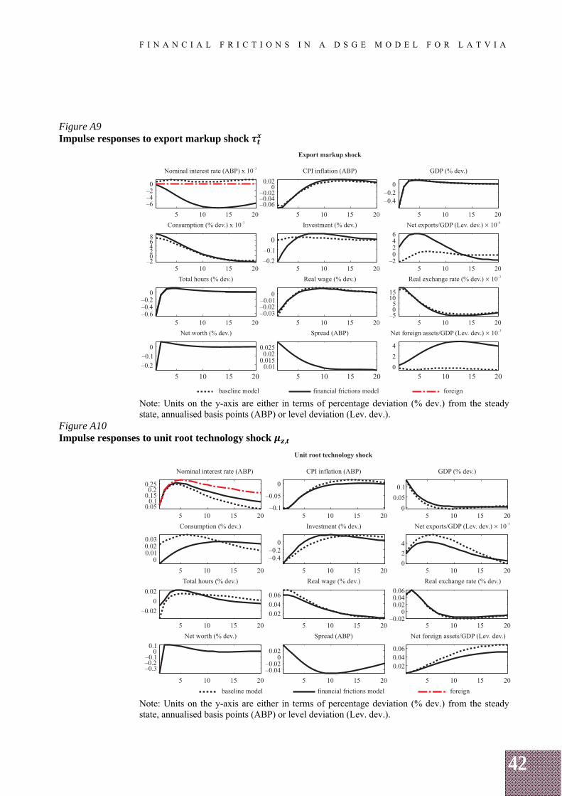
42
F I N A N C I A L F R I C T I O N S I N A D S G E M O D E L F O R L A T V I A
Figure A9 Impulse responses to export markup shock
Note: Units on the y-axis are either in terms of percentage deviation (% dev.) from the steady state, annualised basis points (ABP) or level deviation (Lev. dev.).
Figure A10 Impulse responses to unit root technology shock ,
Note: Units on the y-axis are either in terms of percentage deviation (% dev.) from the steady state, annualised basis points (ABP) or level deviation (Lev. dev.).
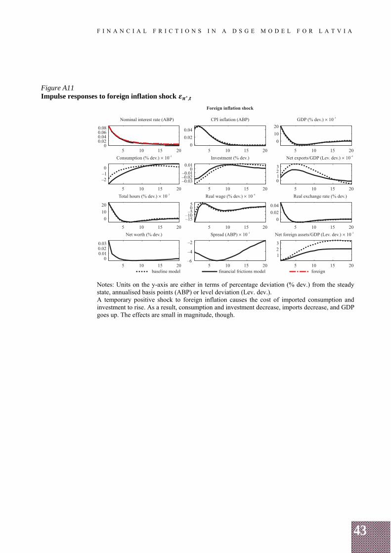
43
F I N A N C I A L F R I C T I O N S I N A D S G E M O D E L F O R L A T V I A
Figure A11 Impulse responses to foreign inflation shock ∗,
Notes: Units on the y-axis are either in terms of percentage deviation (% dev.) from the steady state, annualised basis points (ABP) or level deviation (Lev. dev.). A temporary positive shock to foreign inflation causes the cost of imported consumption and investment to rise. As a result, consumption and investment decrease, imports decrease, and GDP goes up. The effects are small in magnitude, though.
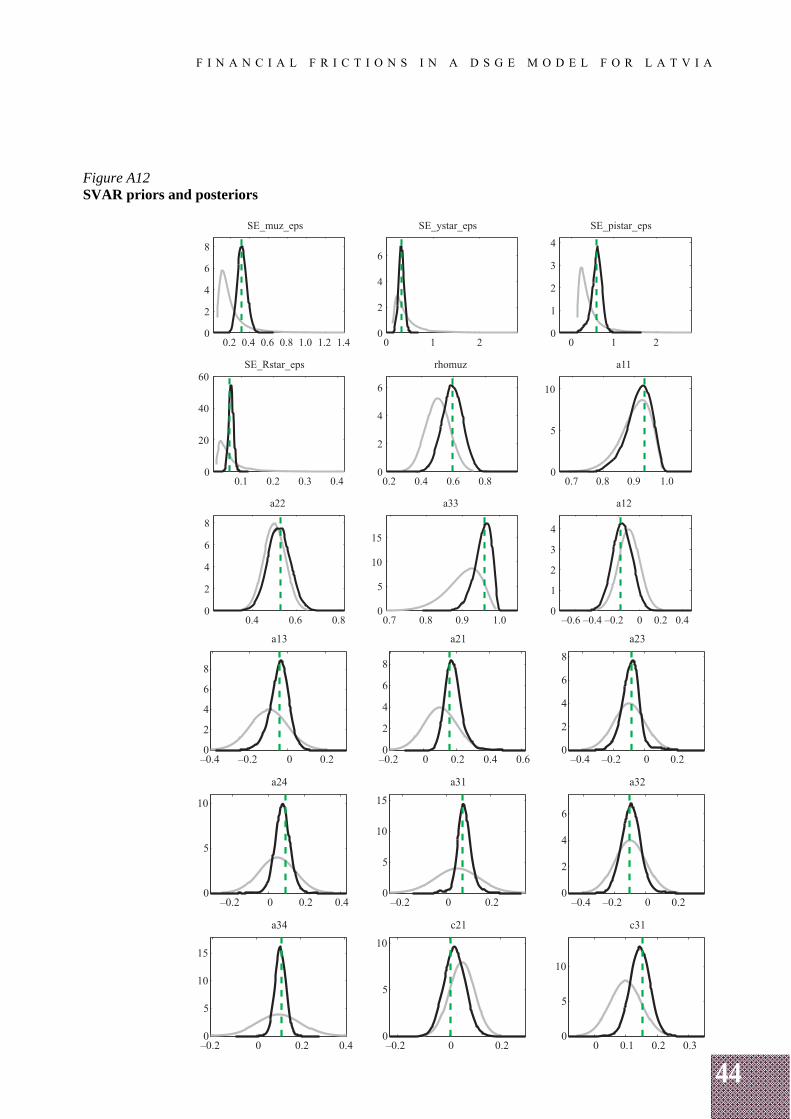
44
F I N A N C I A L F R I C T I O N S I N A D S G E M O D E L F O R L A T V I A
Figure A12 SVAR priors and posteriors
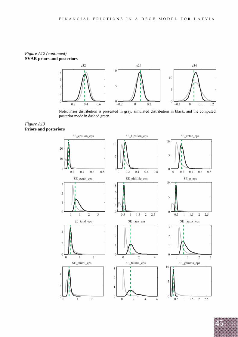
45
F I N A N C I A L F R I C T I O N S I N A D S G E M O D E L F O R L A T V I A
Figure A12 (continued) SVAR priors and posteriors
Note: Prior distribution is presented in gray, simulated distribution in black, and the computed posterior mode in dashed green.
Figure A13 Priors and posteriors
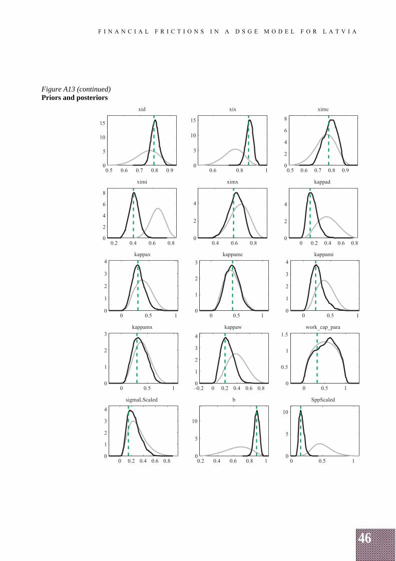
46
F I N A N C I A L F R I C T I O N S I N A D S G E M O D E L F O R L A T V I A
Figure A13 (continued) Priors and posteriors
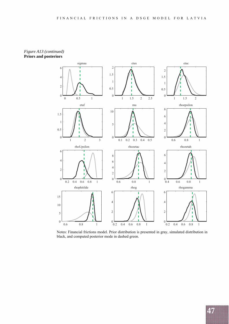
47
F I N A N C I A L F R I C T I O N S I N A D S G E M O D E L F O R L A T V I A
Figure A13 (continued) Priors and posteriors
Notes: Financial frictions model. Prior distribution is presented in gray, simulated distribution in black, and computed posterior mode in dashed green.
48
F I N A N C I A L F R I C T I O N S I N A D S G E M O D E L F O R L A T V I A
Appendix B
MODEL
B.1 Baseline model
As described in Section 2, the three final goods – consumption, investment and exports – are produced by combining the domestic homogeneous good with specific imported inputs for each type of final good. Below we start the model description by going through the production of all these goods.
B.1.1 Production of domestic homogeneous good
A homogeneous domestic good is produced using
,/ , 1 ∞ [1]
where , denotes intermediate goods and 1/ their degree of substitutability. The homogeneous domestic good is produced by a competitive, representative firm which takes the price of output and the price of inputs , as given.
The -th intermediate good producer has the following production function:
, , , ϕ [2]
where , denotes capital services rented by the -th intermediate good producer. Also, log is a technology shock whose first difference has a positive mean, log is a stationary neutral technology shock, and ϕ denotes a fixed production cost. The economy has two sources of growth: the positive drift in log and a positive drift in logΨ where Ψ is an investment-specific technology shock. Object in [2] is defined as13
Ψ .
In [2], , denotes homogeneous labour services hired by -th intermediate good producer.
Firms must borrow fraction of the wage bill, so that one unit of labour costs is denoted by
with
1 [3]
where is the aggregate wage rate, and is the risk-free interest rate that applies to working capital loans.
13 Details regarding the scaling of variables are collected in Appendix D.
49
F I N A N C I A L F R I C T I O N S I N A D S G E M O D E L F O R L A T V I A
The firm's marginal cost, divided by the price of the homogeneous good is denoted by :
[4]
where is the nominal rental rate of capital scaled by and / . Also, is a tax-like shock which affects marginal cost but does not appear in a production function.14
Productive efficiency dictates that marginal cost is equal to marginal cost:
,
,
, ,
[5].
The -th firm is a monopolist in the production of -th good and so it sets its price. Price setting is subject to Calvo frictions. With probability the intermediate good's firm cannot reoptimise its price, in which case
, , , , , : ù ù
where , ù , ù ∈ 0,1 are parameters, is lagged inflation rate and is central bank's (implicit) target inflation rate. Also, is a scalar which allows to capture, among other things, the case in which non-optimising firms either do not change the price at all (i.e., ù 1) or index it only to the steady state inflation rate (i.e., , ù 1). Note that there is a price dispersion in the steady state, if ù 0 and is different from the steady state value of .
With probability 1 the firm can change the price. The problem of -th domestic intermediate good producer, which has the opportunity to change the price, is to maximise discounted profits:
∑ , , , [6],
subject to the requirement that production equals demand. In the above expression, is the multiplier on the household's nominal budget constraint. It measures the
marginal value to the household of one unit of profits in terms of currency. In the steady state when the firm can reoptimise the price, it does so to maximise its discounted profits, subject to price setting frictions and to the requirement that it satisfies the demand given by
,, [7].
The equilibrium conditions associated with the price setting problem and their derivation are reported in Appendix D.
14 In linearised version of the model in which there are no price and wage distortions in the steady state, is isomorphic to a disturbance in , i.e. a markup shock.

50
F I N A N C I A L F R I C T I O N S I N A D S G E M O D E L F O R L A T V I A
The domestic intermediate output good is allocated among alternative uses as follows:
, [8]
where denotes government consumption (which consists entirely of the domestic good), denotes intermediate goods used to produce final household consumption goods (together with foreign consumption goods), is the amount of intermediate domestic goods used in combination with imported foreign investment goods to produce a homogeneous investment good. Finally, the integral in [8] denotes domestic resources allocated to exports. Determination of consumption, investment and export demand is discussed below.
B.1.2 Production of final consumption and investment goods
Final consumption goods are purchased by households. These goods are produced by a representative competitive firm using the following linear homogeneous technology:
1 [9].
The representative firm takes the price of final consumption goods output as exogenous. Final consumption goods output is produced using two inputs. The first
is a one-for-one transformation of the homogeneous domestic good and therefore has price . The second input is the homogeneous composite of specialised consumption import goods discussed in the next subsection. The price of is
, . The representative firm takes the input prices and , as exogenous. Profit maximisation leads to the following demand for intermediate inputs in a scaled form:
1
, [10]
where / and , , / . The price of is related to the price of inputs by
1 , [11].
The rate of inflation of the consumption good is
,
, [12].
Investment goods are produced by a representative competitive firm using the following technology:
Ψ 1
51
F I N A N C I A L F R I C T I O N S I N A D S G E M O D E L F O R L A T V I A
where investment is defined as the sum of investment goods used in the accumulation of physical capital and investment goods used in capital maintenance
. The maintenance is discussed below. See Appendix D for functional form of . denotes utilisation rate of capital, with capital services being defined by
.
In order to accommodate the possibility that the price of investment goods relative to the price of consumption goods declines over time, it is assumed that the investment specific technology shock Ψ is a unit root process with a potentially positive drift. As in the consumption goods sector, the representative investment goods producers take all relevant prices as exogenous. Profit maximisation leads to the following demand for intermediate inputs in a scaled form:
, ,1 [13],
,, ,
[14]
where Ψ / and , , / .
The price of is related to the price of inputs by
1 , [15].
The rate of inflation of the investment good is
,
,
, [16].
B.1.3 Exports and imports
Both export and import activities involve the Calvo price setting frictions and therefore require the presence of monopoly power. The Dixit–Stiglitz strategy is used to introduce a range of specialised goods. This allows there the presence of market power without a counterfactual implication that there is a small number of firms in the export and import sectors. Thus, exports involve a continuum of exporters, each of whom is a monopolist producing a specialised export good. Each monopolist produces the export good using a homogeneous domestically produced good and a homogeneous good derived from imports. Specialised export goods are sold to foreign competitive retailers who create a homogeneous good that is sold to foreign citizens.
In the case of imports, specialised domestic importers purchase a homogeneous foreign good which they turn into a specialised input and sell to domestic retailers. There are three types of domestic retailers. One uses specialised import goods to create a homogeneous good used as an input into the production of specialised exports. The second uses specialised import goods to create an input used in the production of investment goods. The third uses specialised imports to produce a homogeneous input used in the production of consumption goods. Imported goods are combined with domestic inputs before being passed onto final domestic users.
52
F I N A N C I A L F R I C T I O N S I N A D S G E M O D E L F O R L A T V I A
There are pricing frictions in both exports and imports. In all cases it is assumed that prices are set in the currency of the buyer.15
Exports
There is a total demand by foreigners for domestic exports which takes on the following form:
∗∗ [17]
where ∗ is foreign GDP, ∗ is the foreign currency price of foreign homogeneous goods, and is an index of export prices defined below. Goods are produced by a representative competitive foreign retailer firm using specialised inputs as follows:
, [18]
where , , ∈ 0,1 are specialised intermediate goods for export goods production. The retailer producing takes its output price and its input prices , as given. Optimisation leads to the following demand for specialised exports:
,, [19].
Combining [18] and [19] gives
, .
The -th specialised export is produced by a monopolist using the following technology:
, , 1 ,
where , and , are the -th exporter's use of imported and domestically produced goods respectively. The marginal cost associated with the constant elasticity of substitution production function is derived from the multiplier associated with the Lagrangian representation of the cost minimisation problem:
min ,, ,
, , 1 ,
15 Pricing frictions in imports help the model account for the evidence that exchange rate shocks take time to pass into domestic prices. Pricing frictions in exports help the model produce a hump-shape in the response of output to a domestic monetary shock, though, as seen in Section 4, it is not the case for a currency area-wide monetary policy shock.
53
F I N A N C I A L F R I C T I O N S I N A D S G E M O D E L F O R L A T V I A
where , is the price of the homogeneous import good and is the price of the homogeneous domestic good. Using the first order conditions of this problem and the production function, the real marginal cost in terms of stationary variables is derived as
, 1 [20]
where
1 [21], ∗
∗ [22],
and denotes the real exchange rate defined as ∗
[23].
From the solution to the same problem, the demand for domestic inputs for export production is
, , 1 [24].
The quantity of the domestic homogeneous good used by specialised exporters is
, ,
which in terms of aggregates is (by plugging [24] into this integral as derived in Appendix D)
, , 1 1 ∗ [25]
where is a measure of price dispersion defined in Appendix D.
Using a similar derivation as for , we obtain
,
,∗ [26].
The -th, ∈ 0,1 , export goods firm takes [19] as its demand curve. This producer sets prices subject to a Calvo sticky price mechanism. With probability , the -th export goods firm cannot reoptimise its price, in which case it updates the price as follows:
, , , ù ù [27]
where , ù , ù ∈ 0,1 .
Equilibrium conditions associated with price setting by exporters that do get to reoptimise their prices are analogous to the ones derived for the domestic intermediate goods producers and are reported in Appendix D.
54
F I N A N C I A L F R I C T I O N S I N A D S G E M O D E L F O R L A T V I A
Imports
Foreign firms sell a homogeneous good to domestic importers. The importers convert the homogeneous good into a specialised input (brand name it) and supply that input monopolistically to domestic retailers. Importers are subject to the Calvo price setting frictions. There are three types of importing firms: 1) a firm producing goods used to produce an intermediate good for the production of consumption, 2) a firm producing goods used to produce an intermediate good for the production of investment, and 3) a firm producing goods used to produce an intermediate good for the production of exports.
The first group of firms shall be considered first. The production function of the domestic retailer of imported consumption goods is
,,
,
where , is the output of the -th specialised producer, and is an intermediate good used in the production of consumption goods. Let , denote the price index of and ,
, be the price of the -th intermediate input. The domestic retailer is competitive and takes , and ,
, as given. The demand curve for specialised inputs is given by the domestic retailer's first order condition necessary for profit maximisation:
,
,
,,
,
,
.
We now turn to the producer of , who takes the previous equation as a demand curve. This producer buys the homogeneous foreign good and converts it one-for-one into the domestic differentiated good , . The intermediate good producer's marginal cost is
, ∗ ,∗ [28]
where
,∗ ∗ ∗ 1 ∗ [29]
where ∗ is the foreign nominal rate of interest.16
As in the homogeneous domestic good sector, , is a tax-like shock which affects marginal costs but does not appear in the production function.17
The total value of imports accounted for by the consumption sector is 16 The notion here is that the intermediate good firm must pay the inputs in foreign currency and as they have no resources of their own at the beginning of the period, they must borrow those resources if they are to buy the foreign inputs needed to produce , . The financing need is in the foreign currency, so the loan is taken in that currency. There is no risk to this working capital loan, because all shocks are realised at the beginning of the period and so there is no uncertainty during the loan period about the realisation of prices and exchange rates. 17 In the linearisation of a version of the model, in which there are no price and wage distortions in the steady state, , is isomorphic to a markup shock.
55
F I N A N C I A L F R I C T I O N S I N A D S G E M O D E L F O R L A T V I A
∗ ,∗ ,,
,
where
,,
,
is a measure of price dispersion in the differentiated good , .
Now the second group of firms is considered. The production function for the domestic retailer of imported investment goods is
,,
,
.
The retailer of imported investment goods is competitive and takes output prices , and input prices ,
, as given.
The producer of the -th intermediate input into the above production function buys the homogeneous foreign good and converts it one-for-one into the differentiated good , . The marginal cost of , is the analogue of [28]
, ∗ ,∗,
which implies that the importing firm's cost is ∗ (before borrowing costs, exchange rate conversion and markup shocks), which is the same cost for the specialised inputs used to produce .
The total value of imports associated with the production of investment goods is analogous to what was obtained for the consumption goods sector:
∗ ,∗ ,,
, , , ,,
, [30].
Now the third group will be dealt with. The production function of the domestic retailer of imported goods used in the production of input for the production of export goods is
,,
,
.
The imported goods retailer is competitive and takes output prices , and input prices ,
, as given. The producer of specialised input , has marginal cost
, ∗ ,∗.
The total value of imports associated with the production of is
∗ ,∗ ,,, , , ,
,
, [31].
56
F I N A N C I A L F R I C T I O N S I N A D S G E M O D E L F O R L A T V I A
Each of the above three types of intermediate goods firms is subject to the Calvo price setting frictions. With probability 1 , , the -th type of firm can reoptimise its price, and with probability , it updates its price according to
,, ,
,, , , : , , , ù , ù , , , , [32].
The equilibrium conditions associated with the price setting by importers are analogous to the ones derived for domestic intermediate goods producers and are reported in Appendix D.
B.1.4 Households
Household preferences are given by
∑ log , [33]
where denotes consumption preference shock, is disutility of labour shock, is the consumption habit parameter, denotes the -th household's supply of labour services, and stands for the inverse Frisch elasticity. The household owns the economy's stock of physical capital. It determines the rate at which the capital stock is accumulated and the rate at which it is utilised. The household also owns the stock of net foreign assets and determines its rate of accumulation.
Wage setting
The specialised labour supplied by households is combined by labour contractors into homogeneous labour services:
, , 1 ∞.
Households are subject to the Calvo wage setting frictions (as in Erceg, Henderson and Levin, 2000). With probability 1 the -th household is able to reoptimise its wages, and with probability it updates its wages according to
, , , [34],
,ù ù [35]
where , ù , ϑ , ù ∈ 0,1 .
Consider the household that has an opportunity to reoptimise its wages at time . We denote this wage rate by . This is not indexed by because the situation of each household that optimises its wages is the same. In choosing the household considers the discounted utility (neglecting currently irrelevant terms in the household objective) of future histories when it cannot reoptimise:
∑ ,, , [36]
where is tax on labour income, is payroll tax, is the multiplier on household's period budget constraint. The demand for the household's labour services, conditional on it having optimised in period and not again since, is
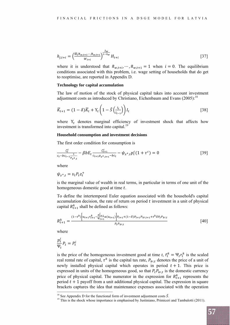
57
F I N A N C I A L F R I C T I O N S I N A D S G E M O D E L F O R L A T V I A
,, ,⋯, , [37]
where it is understood that , , ⋯ , , 1 when 0. The equilibrium conditions associated with this problem, i.e. wage setting of households that do get to reoptimise, are reported in Appendix D.
Technology for capital accumulation
The law of motion of the stock of physical capital takes into account investment adjustment costs as introduced by Christiano, Eichenbaum and Evans (2005):18
1 Υ 1 [38]
where Υ denotes marginal efficiency of investment shock that affects how investment is transformed into capital.19
Household consumption and investment decisions
The first order condition for consumption is
,,
, 1 0 [39]
where
,
is the marginal value of wealth in real terms, in particular in terms of one unit of the homogeneous domestic good at time .
To define the intertemporal Euler equation associated with the household's capital accumulation decision, the rate of return on period investment in a unit of physical capital shall be defined as follows:
, ,
, [40]
where
Ψ
is the price of the homogeneous investment good at time t, Ψ is the scaled real rental rate of capital, is the capital tax rate, , denotes the price of a unit of newly installed physical capital which operates in period 1. This price is expressed in units of the homogeneous good, so that , is the domestic currency price of physical capital. The numerator in the expression for represents the period 1 payoff from a unit additional physical capital. The expression in square brackets captures the idea that maintenance expenses associated with the operation 18 See Appendix D for the functional form of investment adjustment costs . 19 This is the shock whose importance is emphasised by Justiniano, Primiceri and Tambalotti (2011).
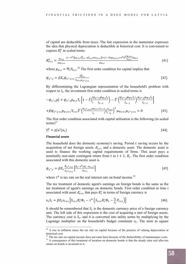
58
F I N A N C I A L F R I C T I O N S I N A D S G E M O D E L F O R L A T V I A
of capital are deductible from taxes. The last expression in the numerator expresses the idea that physical depreciation is deductible at historical cost. It is convenient to express in scaled terms:
,
,,
,
, [41]
where , Ψ , .20 The first order condition for capital implies that
, ,,
[42].
By differentiating the Lagrangian representation of the household's problem with respect to , the investment first order condition in scaled terms is
, , , Υ 1 , , ′ , , , ,
, , Υ ′ , ,, , 0 [43].
The first order condition associated with capital utilisation is the following (in scaled terms)21
′ [44].
Financial assets
The household does the domestic economy's saving. Period saving occurs by the acquisition of net foreign assets ∗ and a domestic asset. The domestic asset is used to finance the working capital requirements of firms. This asset pays a nominally non-state contingent return from to 1, . The first order condition associated with this domestic asset is
,,
, [45]
where is tax rate on the real interest rate on bond income.22
The tax treatment of domestic agent's earnings on foreign bonds is the same as the tax treatment of agent's earnings on domestic bonds. First order condition at time t associated with asset ∗ that pays ∗ in terms of foreign currency is
∗Φ ∗Φ [46].
It should be remembered that is the domestic currency price of a foreign currency unit. The left side of this expression is the cost of acquiring a unit of foreign assets. The currency cost is , and it is converted into utility terms by multiplying by the Lagrange multiplier on the household's budget constraint . The term in square
20 A rise in inflation raises the tax rate on capital because of the practice of valuing depreciation at historical cost. 21 The tax rate on capital income does not enter here because of the deductibility of maintenance costs. 22 A consequence of this treatment of taxation on domestic bonds is that the steady state real after-tax return on bonds is invariant to .
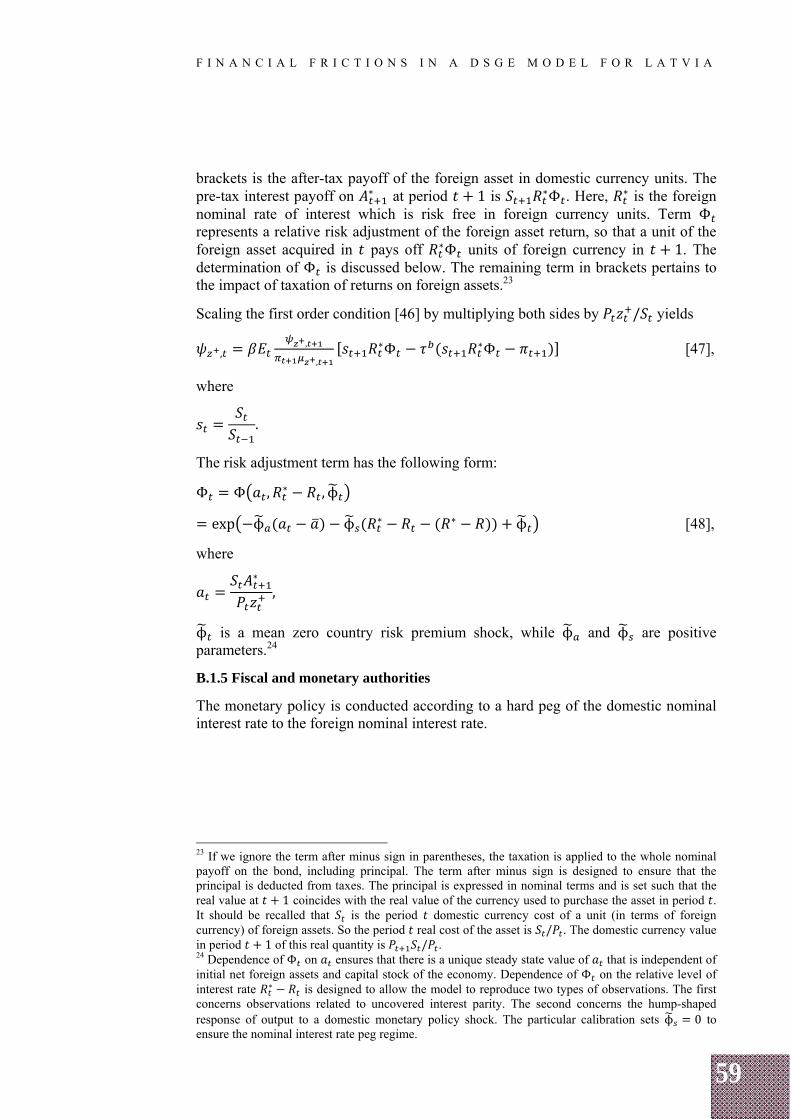
59
F I N A N C I A L F R I C T I O N S I N A D S G E M O D E L F O R L A T V I A
brackets is the after-tax payoff of the foreign asset in domestic currency units. The pre-tax interest payoff on ∗ at period 1 is ∗Φ . Here, ∗ is the foreign nominal rate of interest which is risk free in foreign currency units. Term Φ represents a relative risk adjustment of the foreign asset return, so that a unit of the foreign asset acquired in pays off ∗Φ units of foreign currency in 1. The determination of Φ is discussed below. The remaining term in brackets pertains to the impact of taxation of returns on foreign assets.23
Scaling the first order condition [46] by multiplying both sides by / yields
,,
,
∗Φ ∗Φ [47],
where
.
The risk adjustment term has the following form:
Φ Φ , ∗ , ϕ
exp ϕ ϕ ∗ ∗ ϕ [48],
where
∗
,
ϕ is a mean zero country risk premium shock, while ϕ and ϕ are positive parameters.24
B.1.5 Fiscal and monetary authorities
The monetary policy is conducted according to a hard peg of the domestic nominal interest rate to the foreign nominal interest rate.
23 If we ignore the term after minus sign in parentheses, the taxation is applied to the whole nominal payoff on the bond, including principal. The term after minus sign is designed to ensure that the principal is deducted from taxes. The principal is expressed in nominal terms and is set such that the real value at 1 coincides with the real value of the currency used to purchase the asset in period . It should be recalled that is the period domestic currency cost of a unit (in terms of foreign currency) of foreign assets. So the period real cost of the asset is / . The domestic currency value in period 1 of this real quantity is / . 24 Dependence of Φ on ensures that there is a unique steady state value of that is independent of initial net foreign assets and capital stock of the economy. Dependence of Φ on the relative level of interest rate ∗ is designed to allow the model to reproduce two types of observations. The first concerns observations related to uncovered interest parity. The second concerns the hump-shaped response of output to a domestic monetary policy shock. The particular calibration sets ϕ 0 to ensure the nominal interest rate peg regime.
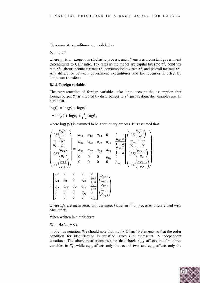
60
F I N A N C I A L F R I C T I O N S I N A D S G E M O D E L F O R L A T V I A
Government expenditures are modeled as
where is an exogenous stochastic process, and ensures a constant government expenditures to GDP ratio. Tax rates in the model are capital tax rate , bond tax rate , labour income tax rate , consumption tax rate , and payroll tax rate . Any difference between government expenditures and tax revenues is offset by lump-sum transfers.
B.1.6 Foreign variables
The representation of foreign variables takes into account the assumption that foreign output ∗ is affected by disturbances to just as domestic variables are. In particular,
log ∗ log ∗ log
log ∗ log log
where log ∗ is assumed to be a stationary process. It is assumed that
log∗
∗
∗ ∗
∗ ∗
log ,
log,
0 0
1
10 0 0 00 0 0 0
log∗
∗
∗ ∗
∗ ∗
log ,
log,
∗ 0 0 0 0
∗ 0
∗
0 0 0 00 0 0 0
∗,∗,∗,
,
,
where 's are mean zero, unit variance, Gaussian i.i.d. processes uncorrelated with each other.
When written in matrix form,
∗ ∗
in obvious notation. We should note that matrix has 10 elements so that the order condition for identification is satisfied, since ′ represents 15 independent equations. The above restrictions assume that shock ∗, affects the first three variables in ∗, while ∗, affects only the second two, and ∗, affects only the
61
F I N A N C I A L F R I C T I O N S I N A D S G E M O D E L F O R L A T V I A
third.25 Also, zeros in the last two columns of the first row in and imply that technology shocks do not affect ∗.26 Third, and matrices capture the notion that innovations to technology affect foreign inflation and interest rate via their impact
on . Fourth, the assumptions on and imply that log , and log , are
univariate first order autoregressive processes driven by , and , respectively.
B.1.7 Resource constraints
The fact that there is a potentially steady state price dispersion both in prices and wages complicates the expression for the domestic homogeneous good in terms of aggregate factors of production. The relationship derived in Appendix D can be expressed as
, ∗,ϕ [49]
where denotes the degree of price dispersion in the intermediate domestic good.
Resource constraint for domestic homogeneous output
Above we defined real scaled output in terms of aggregate factors of production. It is convenient also to have an expression that exhibits the usage of domestic homogeneous output. Using [25],
, 1 1 ∗
or, after scaling by and using [10]
1, ,
1
, 1 1 ∗ [50].
When GDP is matched to the data, capital utilisation costs are subtracted from (see Appendix D):
, ,
1 .
Trade balance
Expenses on imports and new purchases of net foreign assets ∗ must equal income from exports and previously purchased net foreign assets:
∗ ∗ Φ ∗.
25 The assumption about ∗, corresponds to one strategy for identifying a monetary policy shock, in which it is assumed that inflation and output are predetermined relative to the monetary policy shock. 26 This reflects the assumption that the impact of technology shocks on ∗ is completely taken into account by , while other shocks to ∗ are orthogonal to and affect ∗ via ∗.
62
F I N A N C I A L F R I C T I O N S I N A D S G E M O D E L F O R L A T V I A
Expenses on imports correspond to purchases of specialised importers for the consumption, investment and export sectors:27
∗ ,∗ ,,, ,
,
,
, , 1 , .
Current account can be written in a scaled form using [22] as follows:
,∗ ,,
, ,,
, ,,
,
∗ Φ, [51]
where ∗ / .
This completes the description of the baseline model. Additional equilibrium conditions and a complete list of endogenous variables are presented in Appendix D.
B.2 Financial frictions in the model
B.2.1 Overview of financial frictions model
A number of activities in the baseline model require financing. Producers of specialised inputs must borrow working capital within the period. The management of capital involves financing, because the construction of capital requires a substantial initial outlay of resources, while the return from capital comes in over time as a flow. In the baseline model financing requirements affect the allocations, but not very much. This is because none of the messy realities of actual financial markets are present. There is no asymmetric information between the borrower and the lender, there is no risk to lenders. In the case of capital accumulation, the borrower and the lender are actually the same household. When real-world financial frictions are introduced into the model, intermediation becomes distorted by the presence of balance sheet constraints and other factors.
This subsection assumes that accumulation and management of capital involves frictions following BGG (1999). It is assumed that working capital loans are frictionless.
It has already been stated that households deposit money with banks and that interest rate received by households is nominally non-state-contingent. This gives rise to potentially interesting wealth effects of the sort emphasised by Fisher (1933). Banks then lend funds to entrepreneurs using a standard nominal debt contract, which is optimal given the asymmetric information. The amount that banks are willing to lend to an entrepreneur under a standard debt contract is a function of the 27 Note the presence of price distortion terms here. To understand these terms, recall that, e.g. is produced as a linear homogeneous function of specialised imported goods. Because the specialised importers only buy foreign goods, it is their total expenditures that are of interest for us here. When imports are distributed evenly across differentiated goods, the total quantity of those imports is , and the value of imports associated with domestic production of consumption goods is ∗ ,∗ . When there is price distortion among imported intermediate goods, the sum of homogeneous import goods is higher for any given value of .
63
F I N A N C I A L F R I C T I O N S I N A D S G E M O D E L F O R L A T V I A
entrepreneur's net worth. This is how balance sheet constraints enter the model. When a shock that reduces the value of entrepreneur's assets occurs, it cuts into their ability to borrow. As a result, they acquire less capital, and this translates into a reduction in investment and, ultimately, into a slowdown in the economy.
Although individual entrepreneurs are risky, banks themselves are not. It is supposed that banks lend to a sufficiently diverse group of entrepreneurs that the uncertainty that exists in individual entrepreneurial loans washes out across all loans. Net worth of entrepreneurs is empirically measured by using a stock market index.
Entrepreneurs all have different histories, as they experience different idiosyncratic shocks. Thus, in general, solving for the aggregate variables would require also solving for the distribution of entrepreneurs according to their characteristics and for the law of motion for that distribution. However, as emphasised in BGG, the right functional form assumption has been made in the model to guarantee the result that aggregate variables associated with entrepreneurs are not a function of distributions. The loan contract specifies that all entrepreneurs, regardless of their net worth, receive the same interest rate. Also, the loan amount received by an entrepreneur is proportional to his level of net worth. These characteristics are sufficient to guarantee the aggregation result. Financial frictions result in a net increase of two equations over the equations in the baseline model. In addition, they introduce two new endogenous variables, one related to the interest rate paid by entrepreneurs and the other to their net worth. Financial frictions also allow us to introduce two new shocks. A formal discussion of the model follows.
B.2.2 Individual entrepreneur
At the end of period , each entrepreneur has a level of net worth . The entrepreneur's net worth constitutes his state at this time, and nothing else about his history is relevant. There are many entrepreneurs for each level of net worth, and for each level of net worth there is a competitive bank with free entry that offers a loan contract. The contract is defined by the loan amount and interest rate, both of which are derived as the solution to a particular optimisation problem.
Let us consider a type of entrepreneur with particular level of net worth . The entrepreneur combines this net worth with a bank loan to purchase new installed physical capital from capital producers. The loan the entrepreneur requires for this is
, [52].
The entrepreneur is required to pay gross interest rate on the bank loan at the end of period 1, if it is feasible to do so. After purchasing capital, the entrepreneur experiences an idiosyncratic productivity shock, which converts purchased capital into where is a unit mean, log-normally and independently distributed random variable across entrepreneurs with log . The subscript indicates that itself is the realisation of a random variable. This allows us to consider the effects of an increase in the riskiness of individual entrepreneurs, and is designated as the shock to idiosyncratic uncertainty. The cumulative distribution function of is denoted by ; and its partial derivatives by ; and ; .
64
F I N A N C I A L F R I C T I O N S I N A D S G E M O D E L F O R L A T V I A
After observing period 1 shocks, the entrepreneur sets utilisation rate of capital and rents out capital in competitive markets at nominal rental rate . In choosing capital utilisation rate, the entrepreneur takes into account that operating one unit of physical capital at rate requires of domestically produced investment goods for maintenance expenditures, where is defined in Appendix D. The entrepreneur then sells the undepreciated part of physical capital to capital producers. Per unit of physical capital purchased, the entrepreneur who draws idiosyncratic productivity earns a return (after taxes) of , with defined in [40]. Because the mean of across entrepreneurs is unity, the average return across all entrepreneurs is .
After entrepreneurs sell their capital, they settle their bank loans. At this point, the resources available to an entrepreneur who has purchased units of physical capital in period and who experiences an idiosyncratic productivity shock are
, . There is a cutoff value of , such that the entrepreneur has just enough resources to pay interest:
, [53].
Entrepreneurs with are bankrupt and turn over all their resources
, ,
which is less than , to the bank. In this case, the bank monitors the entrepreneur at the cost
,
where 0 is a parameter.
Banks obtain the funds loaned in period to entrepreneurs by issuing deposits to households at gross nominal rate of interest . The subscript in indicates that the payoff to households in 1 is not contingent on period 1 uncertainty. There is no risk in household bank deposits, and the household Euler equation associated with deposits is exactly the same as in [45].
There is competition and free entry among banks, and banks participate in no financial arrangements other than liabilities issued to households and loans issued to entrepreneurs. It follows that the bank's cash flow in each state of period 1 is zero for each loan amount.28 For loan amount , the bank receives gross interest
from fraction 1 ; of entrepreneurs who are not bankrupt. The bank takes all the resources possessed by bankrupt entrepreneurs, net of monitoring costs. Thus, the state-by-state zero profit condition is
1 ; 1 ; ,
or, after making use of [53] and rearranging,
28 Absence of state contingent securities markets guarantees that cash flow is non-negative. Free entry guarantees that ex ante profits are zero. Given that each state receives positive probability, the two assumptions imply the state-by-state zero profit condition.
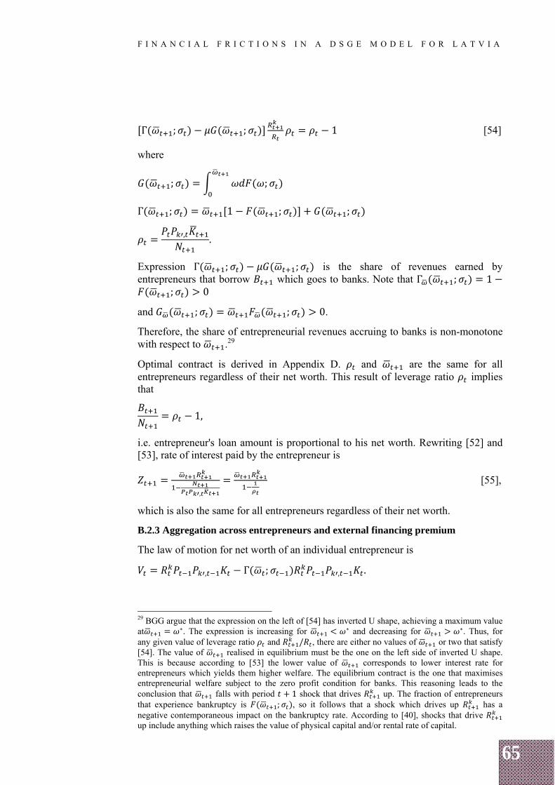
65
F I N A N C I A L F R I C T I O N S I N A D S G E M O D E L F O R L A T V I A
Γ ; ; 1 [54]
where
; ;
Γ ; 1 ; ;
, .
Expression Γ ; ; is the share of revenues earned by entrepreneurs that borrow which goes to banks. Note that Γ ; 1
; 0
and ; ; 0.
Therefore, the share of entrepreneurial revenues accruing to banks is non-monotone with respect to .29
Optimal contract is derived in Appendix D. and are the same for all entrepreneurs regardless of their net worth. This result of leverage ratio implies that
1,
i.e. entrepreneur's loan amount is proportional to his net worth. Rewriting [52] and [53], rate of interest paid by the entrepreneur is
,
[55],
which is also the same for all entrepreneurs regardless of their net worth.
B.2.3 Aggregation across entrepreneurs and external financing premium
The law of motion for net worth of an individual entrepreneur is
, Γ ; , .
29 BGG argue that the expression on the left of [54] has inverted U shape, achieving a maximum value at ∗. The expression is increasing for ∗ and decreasing for ∗. Thus, for any given value of leverage ratio and / , there are either no values of or two that satisfy [54]. The value of realised in equilibrium must be the one on the left side of inverted U shape. This is because according to [53] the lower value of corresponds to lower interest rate for entrepreneurs which yields them higher welfare. The equilibrium contract is the one that maximises entrepreneurial welfare subject to the zero profit condition for banks. This reasoning leads to the conclusion that falls with period 1 shock that drives up. The fraction of entrepreneurs that experience bankruptcy is ; , so it follows that a shock which drives up has a negative contemporaneous impact on the bankruptcy rate. According to [40], shocks that drive up include anything which raises the value of physical capital and/or rental rate of capital.

66
F I N A N C I A L F R I C T I O N S I N A D S G E M O D E L F O R L A T V I A
Each entrepreneur faces an identical and independent probability 1 of being selected to exit the economy. With the probability , each entrepreneur remains in the economy. As the selection is random, net worth of those entrepreneurs who survive is . A fraction 1 of new entrepreneurs arrives. The entrepreneurs who survive or who are new arrivals receive a transfer . This ensures that all entrepreneurs, whether new arrivals or survivors having experienced bankruptcy, have sufficient funds to obtain loans at least in some amount.The average net worth across all entrepreneurs after transfers have been made and exits and entries have occurred, is , or
,
; ,
,
, [56]
where the upper bar over a letter denotes its aggregate average value. Because of its direct effect on entrepreneurial net worth, is referred to as the shock to net worth. For a derivation of the aggregation across entrepreneurs, see Appendix D.
We now turn to the external financing premium for entrepreneurs. The cost of internal funds for the entrepreneur (i.e. his own net worth) is interest rate , which he loses by applying it to capital rather than buying a risk-free domestic asset. The average payment to the bank by all entrepreneurs is the entire object in square brackets in [56]. Thus the term involving represents the excess of external funds over the internal cost of funds. As a result, this is one measure of financing premium in the model. Another is , the excess over the risk-free rate of interest rate paid by entrepreneurs who are not bankrupt. In this paper, it is called the interest rate spread.
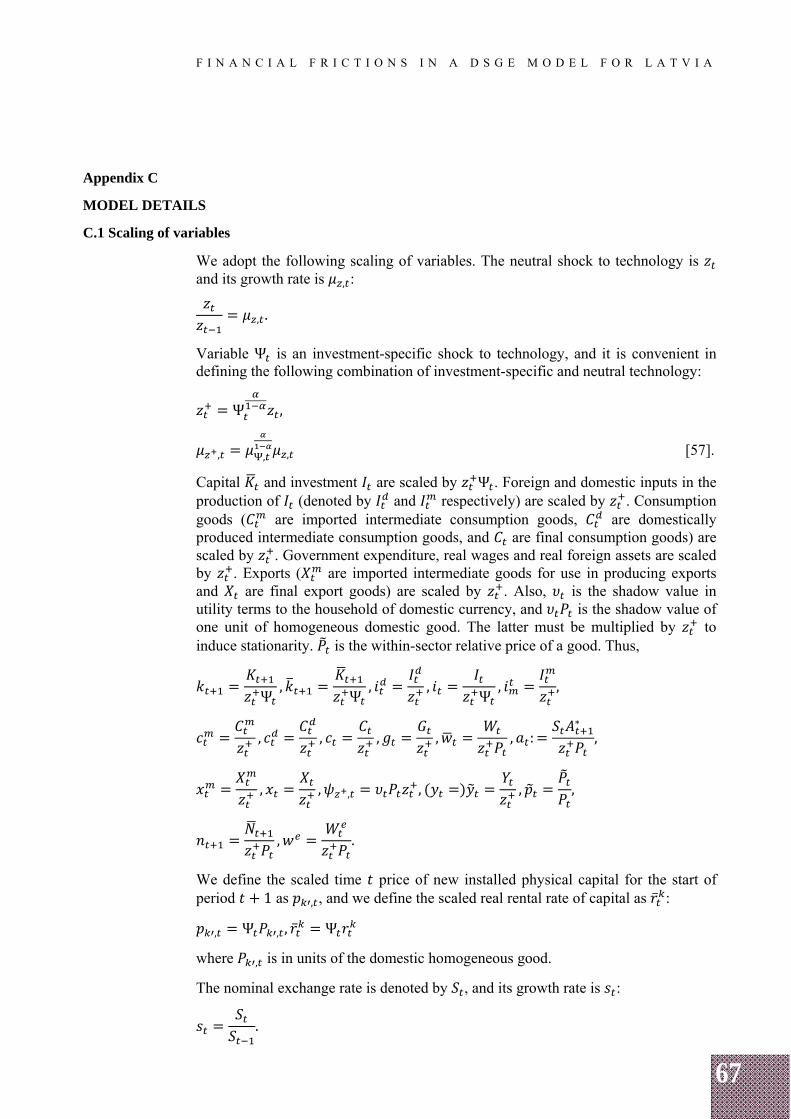
67
F I N A N C I A L F R I C T I O N S I N A D S G E M O D E L F O R L A T V I A
Appendix C
MODEL DETAILS
C.1 Scaling of variables
We adopt the following scaling of variables. The neutral shock to technology is and its growth rate is , :
, .
Variable Ψ is an investment-specific shock to technology, and it is convenient in defining the following combination of investment-specific and neutral technology:
Ψ ,
, , , [57].
Capital and investment are scaled by Ψ . Foreign and domestic inputs in the production of (denoted by and respectively) are scaled by . Consumption goods ( are imported intermediate consumption goods, are domestically produced intermediate consumption goods, and are final consumption goods) are scaled by . Government expenditure, real wages and real foreign assets are scaled by . Exports ( are imported intermediate goods for use in producing exports and are final export goods) are scaled by . Also, is the shadow value in utility terms to the household of domestic currency, and is the shadow value of one unit of homogeneous domestic good. The latter must be multiplied by to induce stationarity. is the within-sector relative price of a good. Thus,
Ψ,
Ψ, ,
Ψ, ,
, , , , , :∗
,
, , , , , ,
, .
We define the scaled time price of new installed physical capital for the start of period 1 as , , and we define the scaled real rental rate of capital as :
, Ψ , , Ψ
where , is in units of the domestic homogeneous good.
The nominal exchange rate is denoted by , and its growth rate is :
.
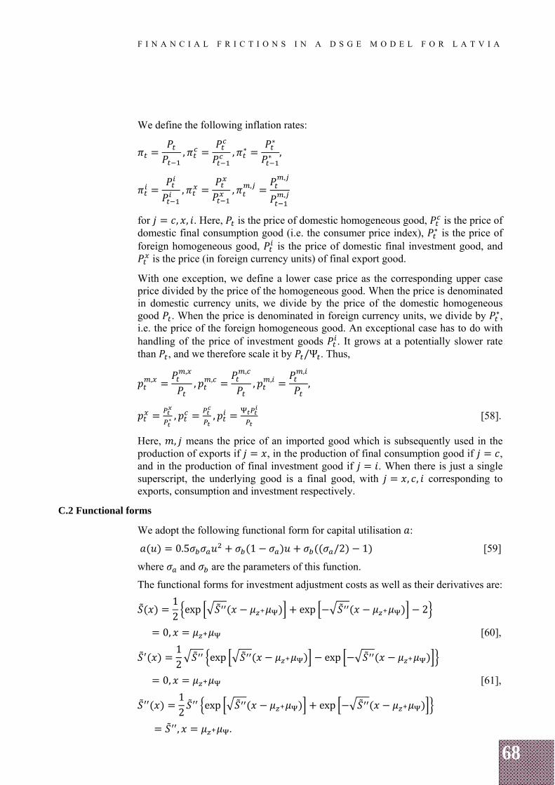
68
F I N A N C I A L F R I C T I O N S I N A D S G E M O D E L F O R L A T V I A
We define the following inflation rates:
, , ∗∗
∗ ,
, , ,,
,
for , , . Here, is the price of domestic homogeneous good, is the price of domestic final consumption good (i.e. the consumer price index), ∗ is the price of foreign homogeneous good, is the price of domestic final investment good, and
is the price (in foreign currency units) of final export good.
With one exception, we define a lower case price as the corresponding upper case price divided by the price of the homogeneous good. When the price is denominated in domestic currency units, we divide by the price of the domestic homogeneous good . When the price is denominated in foreign currency units, we divide by ∗, i.e. the price of the foreign homogeneous good. An exceptional case has to do with handling of the price of investment goods . It grows at a potentially slower rate than , and we therefore scale it by /Ψ . Thus,
,,
, ,,
, ,,
,
∗ , , [58].
Here, , means the price of an imported good which is subsequently used in the production of exports if , in the production of final consumption good if , and in the production of final investment good if . When there is just a single superscript, the underlying good is a final good, with , , corresponding to exports, consumption and investment respectively.
C.2 Functional forms
We adopt the following functional form for capital utilisation :
0.5 1 /2 1 [59]
where and are the parameters of this function.
The functional forms for investment adjustment costs as well as their derivatives are:
12exp exp 2
0, [60],
12
exp exp
0, [61],
12
exp exp
, .
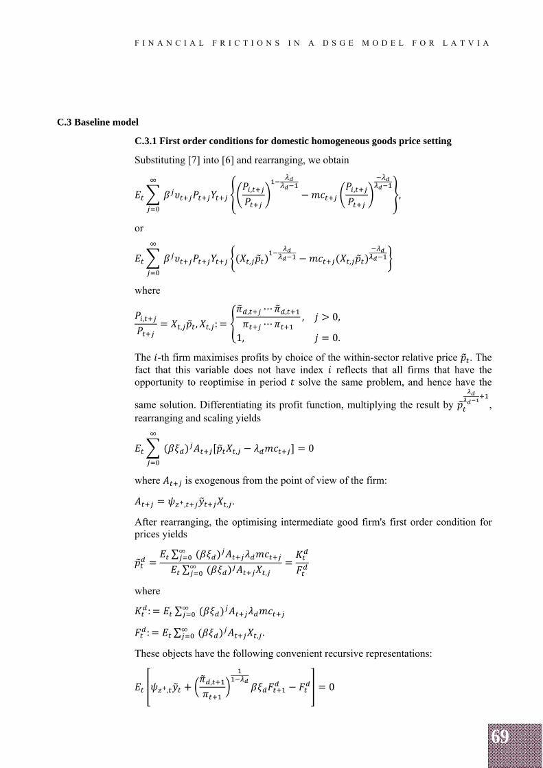
69
F I N A N C I A L F R I C T I O N S I N A D S G E M O D E L F O R L A T V I A
C.3 Baseline model
C.3.1 First order conditions for domestic homogeneous goods price setting
Substituting [7] into [6] and rearranging, we obtain
, , ,
or
, ,
where
,, , , :
, ⋯ ,
⋯, 0,
1, 0.
The -th firm maximises profits by choice of the within-sector relative price . The fact that this variable does not have index reflects that all firms that have the opportunity to reoptimise in period solve the same problem, and hence have the
same solution. Differentiating its profit function, multiplying the result by , rearranging and scaling yields
, 0
where is exogenous from the point of view of the firm:
, , .
After rearranging, the optimising intermediate good firm's first order condition for prices yields
∑ ∑ ,
where
: ∑
: ∑ , .
These objects have the following convenient recursive representations:
,, 0
70
F I N A N C I A L F R I C T I O N S I N A D S G E M O D E L F O R L A T V I A
,, 0.
With respect to the aggregate price index, we write
1 , [62].
After dividing by and rearranging, we get
,
63].
In sum, equilibrium conditions associated with price setting for producers of the domestic homogeneous good are as follows:
,, 0 [64],
,, 0 [65],
1,
, [66],
,
[67],
, : ù ù [68].
C.3.2 Export demand
Scaling [17] yields
∗ [69].
C.3.3 FOCs for export goods price setting
, , , 0 [70],
, , , 0 [71],
71
F I N A N C I A L F R I C T I O N S I N A D S G E M O D E L F O R L A T V I A
1 [72],
,
, [73].
When linearised around the steady state and ù , 0, equations [70]–[73] reduce to
where a hat over a variable indicates log-deviation from the steady state.
C.3.4 Demand for domestic inputs in export production
Integrating [24], we obtain
, 1 ,
1 , [74].
, a linear homogeneous function of , , is defined as:
, .
Then
,
and
, 1 [75]
where
: ,
and the law of motion of is given in [72].
We now simplify [75]. Rewriting the second equality in [20] yields
, 1
or

72
F I N A N C I A L F R I C T I O N S I N A D S G E M O D E L F O R L A T V I A
∗
∗
, 1
or
, 1 .
Substituting into [75] yields
,, 1 1 ∗.
C.3.5 Demand for imported inputs in export production
Scaling [26], yields
,
,∗ [76].
C.3.6 Value of imports of intermediate consumption goods producers
It is of interest to have a measure of the value of imports of intermediate consumption good producers:
∗ ,∗ , .
In order to relate this to C , the demand curve is substituted into the previous expression:
∗ ,∗ ,
,,
,, ∗ ,∗ ,
,, ,
,,
,
∗ ,∗,
,
,,
where
, ,,
,,
,,
.
Thus, the total value of imports accounted for by the consumption sector is
∗ ,∗ ,,, [77]
where ,
,
, .
The derivation for the value of imports used by the investment and export production sectors are analogous.
73
F I N A N C I A L F R I C T I O N S I N A D S G E M O D E L F O R L A T V I A
C.3.7 Marginal costs of importers
Real marginal cost is
, , ∗
,,∗ , ∗
,,∗
,,
,∗ [78]
for , , .
C.3.8 FOCs for imported goods price setting
,, Ξ
,
,
,
, , , , , 0 [79],
, ,, , Ξ ,
,
,
,
,
, , , , 0 [80],
, 1 ,
,
,
,
,
,
,
,
,
,,
,
,
,
,
[81],
,
,
,
,
,
,
, ,
, , [82]
for , , , and where
Ξ .
C.3.9 Wage setting conditions in baseline model
Substituting [37] into the objective function [36], gives
∑
, ⋯ ,
, ⋯ ,, ⋯ , .
74
F I N A N C I A L F R I C T I O N S I N A D S G E M O D E L F O R L A T V I A
Given the rescaled variables,
, ⋯ , , ⋯ ,,
/,
/, ,
where
,
, ⋯ ,
⋯ , ⋯ ,, 0,
1, 0.
It is interesting to investigate the value of , in the steady state, as → ∞. Thus,
,⋯ ⋯ ù ù
⋯ , ⋯ ,.
In the steady state,
,
ù ù
ù
→ 0
in the no-indexing case where 1, ù 1 and ϑ 0.
Simplifying by using the scaling notation, gives
∑ ,
, ,
or
∑ ,
, , ,
or
∑ ,
, , , .
75
F I N A N C I A L F R I C T I O N S I N A D S G E M O D E L F O R L A T V I A
Differentiating with respect to and solving for the wage rate (some math skipped), gives
∑ ,
∑ ,, ,
,
,
where
, : ∑ ,
, : ∑ ,, , .
Thus, the wage set by reoptimising households is
,
,.
We now express , and , in recursive form (some math skipped):
,,
,,
where
,, [83].
Also (some math skipped),
,, ,
,, .
The second restriction on is obtained using the relation between the aggregate wage rate and the wage rates of individual households:
1 , .
Dividing both sides by and rearranging, we obtain
,
, .
Substituting out for from the household's FOC for wage optimisation,
,
,, , .
76
F I N A N C I A L F R I C T I O N S I N A D S G E M O D E L F O R L A T V I A
We now derive the relationship between aggregate homogeneous hours worked and aggregate household hours,
: , .
Substituting the demand for , into the latter expression, gives
,
= ,
[84]
where
, ,
and
1 , ,
so that
1 ,
,
1,
, ,
, [85].
In addition to [85], we have the following equilibrium conditions associated with sticky wages:
,, ,
,, [86],
,,
,, [87],
,
,, , [88].

77
F I N A N C I A L F R I C T I O N S I N A D S G E M O D E L F O R L A T V I A
C.3.10 Scaling law of motion of capital
Using [38], the law of motion of capital in scaled terms is
, ,Υ 1 , ,
[89].
C.3.11 Output and aggregate factors of production
Below we derive a relationship between total output of domestic homogeneous good and aggregate factors of production.
Consider the unweighted average of intermediate goods:
,
, , ϕ
,
,, ϕ
, ϕ
where is the economy-wide average stock of capital services and is the economy-wide average of homogeneous labour. The last expression exploits the fact that all intermediate good firms confront the same factor prices and hence adopt the same capital services to homogeneous labour ratio. This follows from cost minimisation and holds for all firms, regardless of whether or not they have an opportunity to reoptimise. Then
ϕ.
The demand for , is
,
, ,
so that
: , ,
where
, [90].
Dividing by P , we obtain
or
78
F I N A N C I A L F R I C T I O N S I N A D S G E M O D E L F O R L A T V I A
1,
, [91].
The preceding implies that
ϕ
or, after scaling by ,
, ,ϕ
where [92].
Plugging H from [84],
, ,ϕ .
C.3.12 Restrictions across inflation rates
We now consider the restrictions across inflation rates implied by the relative price expressions. In terms of expressions in [58], there are restrictions implied by
, / , , , , , and . Restrictions implied by the other two relative prices in [58] and have already been used in [16] and [89] respectively. Finally, we also use the restriction across inflation rates implied by / and [23]. Thus,
,
,
,
[93],
,
,
,
[94],
,
,
,
[95],
∗ [96],
∗
[97].
C.3.13 Endogenous variables of baseline model
The following 70 equations have been derived above:
[3], [4], [5], [64], [65], [66], [67], [68], [59], [10], [11], [12], [15], [16], [14], [69], [21], [20], [27], [70], [71], [72], [73], [76], [29], [79], [80], [81], [82], [32], [78], [60], [61] [89], [39], [41], [42], [43], [44], [45], [47], [86], [87], [88], [85], [35], [83], [84], [92], [49], [51], [50], [93], [94], [95], [96], [97], [48],
which can be used to solve the following 70 unknowns:
79
F I N A N C I A L F R I C T I O N S I N A D S G E M O D E L F O R L A T V I A
, , ,∗, , , , , , , , , , , , , , , , , , , , , , , , , , , , , , , , , , , , , , , , , , ,
, , , , , , , , , , , , , , , , , , , ,, , , ; , , ,
, , , , , , Φ , , , , , , , , .
C.4 Equilibrium conditions for financial frictions model
C.4.1 Derivation of optimal contract
As noted in the text, it is supposed that the equilibrium debt contract maximises entrepreneurial welfare subject to the zero profit condition on banks and the specified required return on household bank liabilities. Time debt contract specifies the level of debt and state 1-contingent rate of interest . We suppose that entrepreneurial welfare corresponds to entrepreneur's expected wealth at the end of the contract. It is convenient to express welfare as a ratio to the amount the entrepreneur could receive by depositing his net worth in a bank:
, ;
; ,
1 Γ ;
after making use of [52], [53] and
1 ; ; ; .
We can equivalently characterise the contract by a state 1 contingent set of values for and a value of . The equilibrium contract is the one involving
and , which maximises entrepreneurial welfare (relative to ) subject to the bank zero profits condition. The Lagrangian representation of this problem is
max,
1 Γ ; Γ ; ;
1
where is the Lagrange multiplier, which is defined for each period 1 state. FOCs for this problem are
1 Γ ; Γ ; ; 1 0
Γ ; Γ ; ; 0
1 0
where the absence of from the complementary slackness condition reflects the assumption that 0 in each period 1 state. Substituting out for from the second equation into the first, FOCs reduce to
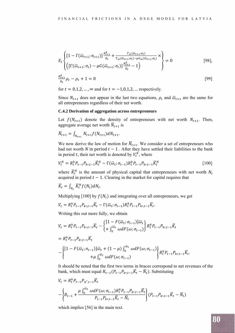
80
F I N A N C I A L F R I C T I O N S I N A D S G E M O D E L F O R L A T V I A
1 Γ ;;
; ;
Γ ; ; 10 [98],
1 0 [99]
for 0,1,2, … ,∞ and for 1,0,1,2, … respectively.
Since does not appear in the last two equations, and are the same for all entrepreneurs regardless of their net worth.
C.4.2 Derivation of aggregation across entrepreneurs
Let denote the density of entrepreneurs with net worth . Then, aggregate average net worth is
.
We now derive the law of motion for . We consider a set of entrepreneurs who had net worth inperiod 1. After they have settled their liabilities to the bank in period , their net worth is denoted by , where
, Γ ; , [100]
where is the amount of physical capital that entrepreneurs with net worth acquired in period 1. Clearing in the market for capital requires that
.
Multiplying [100] by and integrating over all entrepreneurs, we get
, Γ ; , .
Writing this out more fully, we obtain
,
1 ;
; ,
,
1 ; 1 ;
;, .
It should be noted that the first two terms in braces correspond to net revenues of the bank, which must equal , . Substituting
,
; ,
,,
which implies [56] in the main text.
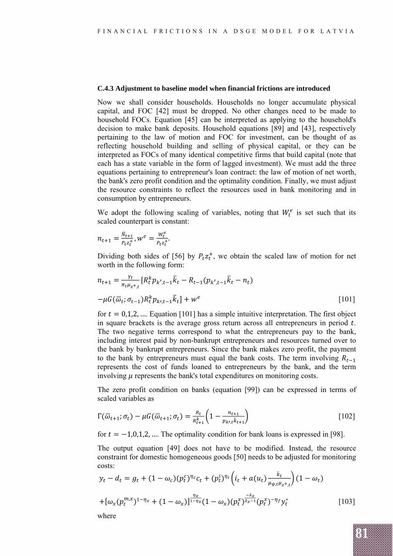
81
F I N A N C I A L F R I C T I O N S I N A D S G E M O D E L F O R L A T V I A
C.4.3 Adjustment to baseline model when financial frictions are introduced
Now we shall consider households. Households no longer accumulate physical capital, and FOC [42] must be dropped. No other changes need to be made to household FOCs. Equation [45] can be interpreted as applying to the household's decision to make bank deposits. Household equations [89] and [43], respectively pertaining to the law of motion and FOC for investment, can be thought of as reflecting household building and selling of physical capital, or they can be interpreted as FOCs of many identical competitive firms that build capital (note that each has a state variable in the form of lagged investment). We must add the three equations pertaining to entrepreneur's loan contract: the law of motion of net worth, the bank's zero profit condition and the optimality condition. Finally, we must adjust the resource constraints to reflect the resources used in bank monitoring and in consumption by entrepreneurs.
We adopt the following scaling of variables, noting that is set such that its scaled counterpart is constant:
, .
Dividing both sides of [56] by , we obtain the scaled law of motion for net worth in the following form:
,, ,
; , [101]
for 0,1,2, …. Equation [101] has a simple intuitive interpretation. The first object in square brackets is the average gross return across all entrepreneurs in period . The two negative terms correspond to what the entrepreneurs pay to the bank, including interest paid by non-bankrupt entrepreneurs and resources turned over to the bank by bankrupt entrepreneurs. Since the bank makes zero profit, the payment to the bank by entrepreneurs must equal the bank costs. The term involving represents the cost of funds loaned to entrepreneurs by the bank, and the term involving represents the bank's total expenditures on monitoring costs.
The zero profit condition on banks (equation [99]) can be expressed in terms of scaled variables as
Γ ; ; 1,
[102]
for 1,0,1,2, …. The optimality condition for bank loans is expressed in [98].
The output equation [49] does not have to be modified. Instead, the resource constraint for domestic homogeneous goods [50] needs to be adjusted for monitoring costs:
1, ,
1
, 1 1 ∗ [103]
where
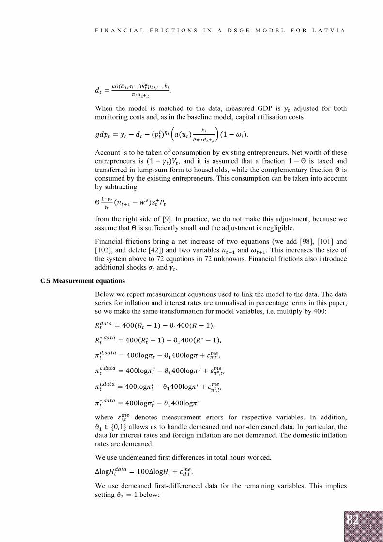
82
F I N A N C I A L F R I C T I O N S I N A D S G E M O D E L F O R L A T V I A
; ,
,.
When the model is matched to the data, measured GDP is adjusted for both monitoring costs and, as in the baseline model, capital utilisation costs
, ,1 .
Account is to be taken of consumption by existing entrepreneurs. Net worth of these entrepreneurs is 1 , and it is assumed that a fraction 1 Θ is taxed and transferred in lump-sum form to households, while the complementary fraction Θ is consumed by the existing entrepreneurs. This consumption can be taken into account by subtracting
Θ
from the right side of [9]. In practice, we do not make this adjustment, because we assume that Θ is sufficiently small and the adjustment is negligible.
Financial frictions bring a net increase of two equations (we add [98], [101] and [102], and delete [42]) and two variables and . This increases the size of the system above to 72 equations in 72 unknowns. Financial frictions also introduce additional shocks and .
C.5 Measurement equations
Below we report measurement equations used to link the model to the data. The data series for inflation and interest rates are annualised in percentage terms in this paper, so we make the same transformation for model variables, i.e. multiply by 400:
400 1 ϑ 400 1 ,
∗, 400 ∗ 1 ϑ 400 ∗ 1 ,
, 400log ϑ 400log , ,
, 400log ϑ 400log , ,
, 400log ϑ 400log , ,
∗, 400log ∗ ϑ 400log ∗
where , denotes measurement errors for respective variables. In addition, ϑ ∈ 0,1 allows us to handle demeaned and non-demeaned data. In particular, the data for interest rates and foreign inflation are not demeaned. The domestic inflation rates are demeaned.
We use undemeaned first differences in total hours worked,
Δlog 100Δlog , .
We use demeaned first-differenced data for the remaining variables. This implies setting ϑ 1 below:
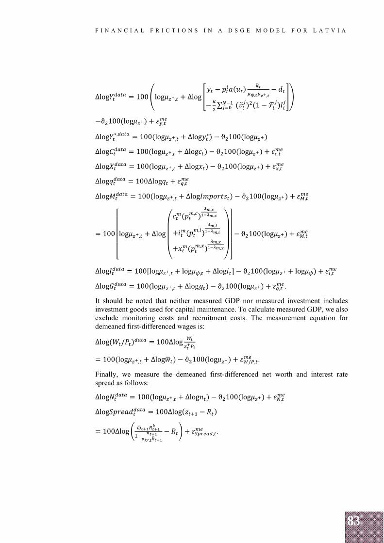
83
F I N A N C I A L F R I C T I O N S I N A D S G E M O D E L F O R L A T V I A
Δlog 100 log , Δlog , ,
∑ 1
ϑ 100 log ,
Δlog ∗, 100 log , Δlog ∗ ϑ 100 log
Δlog 100 log , Δlog ϑ 100 log ,
Δlog 100 log , Δlog ϑ 100 log ,
Δlog 100Δlog ,
Δlog 100 log , Δlog ϑ 100 log ,
100 log , Δlog
,,,
,,
,
,,,
ϑ 100 log ,
Δlog 100 log , log , Δlog ϑ 100 log log ,
Δlog 100 log , Δlog ϑ 100 log , .
It should be noted that neither measured GDP nor measured investment includes investment goods used for capital maintenance. To calculate measured GDP, we also exclude monitoring costs and recruitment costs. The measurement equation for demeaned first-differenced wages is:
Δlog / 100Δlog
100 log , Δlog ϑ 100 log / , .
Finally, we measure the demeaned first-differenced net worth and interest rate spread as follows:
Δlog 100 log , Δlog ϑ 100 log ,
Δlog 100Δlog
100Δlog,
, .
84
F I N A N C I A L F R I C T I O N S I N A D S G E M O D E L F O R L A T V I A
BIBLIOGRAPHY
ADJEMIAN, Stéphane, BASTANI, Houtan, JUILLARD, Michel, KARAMÉ, Frédéric, MIHOUBI, Ferhat, PERENDIA, George, PFEIFER, Johannes, RATTO, Marco, VILLEMOT, Sébastien (2011) – Dynare: Reference Manual, Version 4. Dynare Working Papers, No. 1, CEPREMAP, April. 100 p.
ADOLFSON, Malin, LASÉEN, Stefan, LINDÉ, Jesper, VILLANI, Mattias (2008) – Evaluating an Estimated New Keynesian Small Open Economy Model. Journal of Economic Dynamics and Control, vol. 32, issue 8, August, pp. 2690–2721.
BERNANKE, Ben, GERTLER, Mark, GILCHRIST, Simon (1999) – The Financial Accelerator in a Quantitative Business Cycle Framework. In: Handbook of Macroeconomics, vol. 1. Ed. by John B. Taylor and Michael Woodford. Elsevier Science, pp. 1341–1393.
CHRISTIANO, Lawrence J., EICHENBAUM, Martin, EVANS, Charles L. (2005) – Nominal Rigidities and the Dynamic Effects of a Shock to Monetary Policy. Journal of Political Economy, vol. 113, No. 1, pp. 1–45.
CHRISTIANO, Lawrence J., TRABANDT, Mathias, WALENTIN, Karl (2011) – Introducing Financial Frictions and Unemployment into a Small Open Economy Model. Journal of Economic Dynamics and Control, vol. 35, issue 12, December, pp. 1999–2041.
DIXIT, Avinash K., STIGLITZ, Joseph E. (1977) – Monopolistic Competition and Optimum Product Diversity. American Economic Review, vol. 67, No. 3, June, pp. 297–308.
ERCEG, Christopher J., HENDERSON, Dale W., LEVIN, Andrew T. (2000) – Optimal Monetary Policy with Staggered Wage and Price Contracts. Journal of Monetary Economics, vol. 46, issue 2, October, pp. 281–313.
FISHER, Irving (1933) – The Debt-Deflation Theory of Great Depressions. Econometrica, vol. 1, No. 4, October, pp. 337–357.
JUSTINIANO, Alejandro, PRIMICERI, Giorgio, TAMBALOTTI, Andrea (2011) – Investment Shocks and the Relative Price of Investment. Review of Economic Dynamics, vol. 14, issue 1, January, pp. 101–121.
STEHRER, Robert (2013) – Accounting Relations in Bilateral Value Added Trade. wiiw Working Papers, No. 101, May, The Vienna Institute for International Economic Studies (wiiw).