Financial Frictions, Asset Prices, and the Great Recession · Financial Frictions, Asset Prices,...
65
. . . . . . . . . . . . . . . . . , . . . . . . . . . . . . . Financial Frictions, Asset Prices, and the Great Recession Zhen Huo and Jos´ e-V´ ıctor R´ ıos-Rull University of Minnesota, Federal Reserve Bank of Minneapolis, CAERP, CEPR, NBER University of Mannheim Sept 24, 2013 Very Preliminary Huo & R´ ıos-Rull (UMN, Mpls Fed, CAERP) Financial Frictions & Great Recessions University of Mannheim 1 / 65
Transcript of Financial Frictions, Asset Prices, and the Great Recession · Financial Frictions, Asset Prices,...

.....................
,..........
.....
.
Financial Frictions, Asset Prices, and the GreatRecession
Zhen Huo and Jose-Vıctor Rıos-Rull
University of Minnesota, Federal Reserve Bank of Minneapolis, CAERP, CEPR, NBER
University of MannheimSept 24, 2013
Very Preliminary
Huo & Rıos-Rull (UMN, Mpls Fed, CAERP) Financial Frictions & Great Recessions University of Mannheim 1 / 65

.....................
,..........
.....
.
Facts on the last recession: I
2004 2006 2008 2010 2012−8
−6
−4
−2
0
2
4
6
Real output
2004 2006 2008 2010 20124
5
6
7
8
9
10
Unemployment
2004 2006 2008 2010 2012−10
−8
−6
−4
−2
0
2
4
6
Consumption
2004 2006 2008 2010 2012−40
−30
−20
−10
0
10
20
30
Investment
Note: Except for unemployment, figures show percentage deviation from a linear trend.Huo & Rıos-Rull (UMN, Mpls Fed, CAERP) Financial Frictions & Great Recessions University of Mannheim 2 / 65

.....................
,..........
.....
.
Facts on the last recession: II
2004 2006 2008 2010 20123.6
3.8
4
4.2
4.4
4.6
4.8
5
Wealth to output
2004 2006 2008 2010 20120.55
0.6
0.65
0.7
0.75
0.8
Debt to output
2004 2006 2008 2010 20121
1.1
1.2
1.3
1.4
1.5
1.6
1.7
1.8
Housing value to output
2004 2006 2008 2010 2012160
170
180
190
200
210
220
230
Housing price indexHuo & Rıos-Rull (UMN, Mpls Fed, CAERP) Financial Frictions & Great Recessions University of Mannheim 3 / 65

.....................
,..........
.....
.
Facts on the last recession: III
2004 2006 2008 2010 2012−4
−3
−2
−1
0
1
2
3
TFP with total hours
2004 2006 2008 2010 2012−3
−2
−1
0
1
2
3
4
Labor productivity
2004 2006 2008 2010 2012−1
−0.8
−0.6
−0.4
−0.2
0
0.2
0.4
0.6
0.8
Labor quality2004 2006 2008 2010 2012
−5
−4
−3
−2
−1
0
1
2
3
4
TFP with total labor inputs
Note: Figures show percentage deviation from a linear trend.Huo & Rıos-Rull (UMN, Mpls Fed, CAERP) Financial Frictions & Great Recessions University of Mannheim 4 / 65

.....................
,..........
.....
.
Summary of the facts
Large decline in main aggregate variables.
Households deleveraging process: private debt and housing price plunged.
Total factor productivity dropped, but labor productivity and labor qualityincreased.
Huo & Rıos-Rull (UMN, Mpls Fed, CAERP) Financial Frictions & Great Recessions University of Mannheim 5 / 65

.....................
,..........
.....
.
Objective of this project
To explore the quantitative properties of environments where recessions arecaused by worse financial conditions faced by households.
These environments have
...1 Real frictions that make difficult to switch from production of consumption goodsto exports or investment.
...2 Households differing in wealth and job market prospects.
...3 A financial system used widely by households to buy houses which are inferiorgoods and not wanted by the super-rich.
...4 Asset prices respond to market conditions.
...5 Frictions in the goods market generate movements in measured TFP.
Huo & Rıos-Rull (UMN, Mpls Fed, CAERP) Financial Frictions & Great Recessions University of Mannheim 6 / 65

.....................
,..........
.....
.
Ingredients of this project
It is a small open Aiyagari/Krusell-Smith economy with a housing market and astock market.
Borrowing has to be collateralized by the value of housing. The financial termsavailable are the financial conditions and are subject to shocks.
Like in Huo & Rios-Rull(13) there are goods market frictions that generateTFP losses, job market frictions, and adjustment costs to move into tradableproduction.
Huo & Rıos-Rull (UMN, Mpls Fed, CAERP) Financial Frictions & Great Recessions University of Mannheim 7 / 65

.....................
,..........
.....
.
Findings
A recession can be triggered by financial shocks to households.
It shares most of the features of the Great Recession.
Insufficient reductions in assets (housing and stocks) prices.
For now!!
Huo & Rıos-Rull (UMN, Mpls Fed, CAERP) Financial Frictions & Great Recessions University of Mannheim 8 / 65

.....................
,..........
.....
.
The Model
Huo & Rıos-Rull (UMN, Mpls Fed, CAERP) Financial Frictions & Great Recessions University of Mannheim 9 / 65

.....................
,..........
.....
.
Households: PreferencesContinuum of households that live forever (β), are subject to uninsurableidiosyncratic and aggregate shocks.
Hholds care about quantities and number of varieties of nontradables.
cN =
(∫ IN
0
c1ρ
Ni di
)ρ
Under equal consumption of each variety: cN IρN =
[∫ IN0
c1ρ
Ni di
]ρ
Households have to search for varieties, its number is a choice.
IN = d Ψd(Qg )
Ψd(Qg ): Probability (per search unit) of finding a variety.
Households also like tradables and housing and dislike goods searching
u [cA(cN IρN , cT ), h, d ]
Huo & Rıos-Rull (UMN, Mpls Fed, CAERP) Financial Frictions & Great Recessions University of Mannheim 10 / 65

.....................
,..........
.....
.
Households: Endowments and Wealth
Household skill type is ϵ, follows a Markov chain Γϵ,ϵ′ . Moves slowly andaccommodates opportunities to get rich.
Households either have a job e = 1 or not e = 0.
Type-dependent exogenous job destruction rate δϵn.
Job finding rate is type independent and depends on job creation by firms (workersare rationed, it is like no matching function in labor market but hiring costs) (Fang
and Nie (2013)).
Households have assets a. These assets can be allocated to (frictionless)houses and/or to financial assets with a collateral constraint. The poor willhave some housing wealth and a mortgage, the rich houses and shares of theeconomy’s mutual fund.
Huo & Rıos-Rull (UMN, Mpls Fed, CAERP) Financial Frictions & Great Recessions University of Mannheim 11 / 65

.....................
,..........
.....
.
Production: two sectors tradables and nontradables.
Tradables. Measure one of competitive firms.
(Large) Adjustment costs to both capital and labor.
Its output is used for exports, investment, and (part of) consumption.
FT (k, ℓ) may have decreasing returns.
Nontradables Measure one of monopolistic firms each one producing a different variety.
Each firm/variety has a measure one of locations, each location has its ownproduction function FN(k, ℓ1, ℓ2).⋆ ℓ1 Committed to the location. (Sales staff)⋆ ℓ2 Can be reallocated within the period. (Production Staff )
Locations may or may not be filled (get a customer). They produce only forconsumption.
Firms post prices before the location is filled.
Huo & Rıos-Rull (UMN, Mpls Fed, CAERP) Financial Frictions & Great Recessions University of Mannheim 12 / 65

.....................
,..........
.....
.
Goods markets
• Perfect competition and frictionless markets for tradables.
• Search frictions in the markets for nontradables:
Households look for varieties.
CRS matching function M(D, 1). Market tightness is Qg = 1D .
Random search. There is no possibility of attracting more customers with lowerprices (we are working on a paper where there is shopping and searchingsimultaneously).
The probability that a shopper finds a firm-variety: Ψd(Qg ) = MD
The probability that a firm finds a shopper is the measure of filled locations or ofconsumers buying the good: Ψf (Qg ) = M
1= M(D, 1).
Huo & Rıos-Rull (UMN, Mpls Fed, CAERP) Financial Frictions & Great Recessions University of Mannheim 13 / 65
.....................
,..........
.....
.
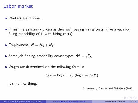
Labor market
Workers are rationed.
Firms hire as many workers as they wish paying hiring costs. (like a vacancyfilling probability of 1, with hiring costs).
Employment: N = NN + NT .
Same job finding probability across types: Φe = V1−N .
Wages are determined via the following formula
logw − logw = εw(logY − logY
)It simplifies things.
Gornemann, Kuester, and Nakajima (2012).
Huo & Rıos-Rull (UMN, Mpls Fed, CAERP) Financial Frictions & Great Recessions University of Mannheim 14 / 65

.....................
,..........
.....
.
Assets markets: Financial assets and houses
Total housing H is in fixed supply.
Negative financial assets (b′ < 0) are (undefaultable) mortgages.
Its interest rate 1qis predetermined at borrowing time,
q(θ, b′) =
1, if b ≥ 0
11+r∗ − ς(θ), if b < 0
Mortgages have to be collateralized by housing
q(θ, b) b ≥ −λ(θ) ph(S) h
Positive financial assets (b > 0) are shares of a mutual fund.
Its return is stochastic. Possible Capital gains and loses.
The return is
R(S , S ′, b) =
1 + r(S , S ′), if b ≥ 01, if b < 0.
Huo & Rıos-Rull (UMN, Mpls Fed, CAERP) Financial Frictions & Great Recessions University of Mannheim 15 / 65

.....................
,..........
.....
.
State variables
A household is characterized by ϵ, e, a.
Let X denote the measure over types x = ϵ, e, a.
The vector of aggregate state variables is
S = θ,B,KN ,KT ,NN ,NT ,X
Here B is the net foreign asset position. K and N are predetermined factorinputs.
Hence either we do Krusell-Smith or the transition after an unforeseen shock.Today, we do the latter.
Huo & Rıos-Rull (UMN, Mpls Fed, CAERP) Financial Frictions & Great Recessions University of Mannheim 16 / 65

.....................
,..........
.....
.
Households’ problem
V (S , ϵ, e, a) = maxcN,i ,cT ,IN ,h,d
u(cA, h, d)+
β∑
ϵ′,e′,θ′
Πθθ,θ′ Πw
e′|e,ϵ(S′) Πε
ϵ,ϵ′ V [S ′, ϵ′, e′, a′(S ′, b, h)]
subject to∫ IN
0
pi (S)cN,i + cT + ph(S)h + q(θ, b)b = a+ 1e=1w(S)ϵ+ 1e=0 w BC
a′(S ′, b, h) = ph(S′)h + R(S , S ′, b)b AA
q(θ, b)b ≥ −λ(θ)ph(S)h FC
IN = d Ψd [Qg (S)] SC
S ′ = G (S , θ′) RE
Huo & Rıos-Rull (UMN, Mpls Fed, CAERP) Financial Frictions & Great Recessions University of Mannheim 17 / 65

.....................
,..........
.....
.
Nontradable firms’ problem
At each location, the production function is
FN(k, ℓ1, ℓ2) = zNkα0ℓα1
1 ℓα22
k and ℓ1 are pre-installed. ℓ2 is variable to meet different demands.
The demand function is given by c(pi , S , x) =[
pip(S)
] ρ1−ρ
cN(S , x)
When a shopper wants to buy c units of goods at a location, the amount ofvariable labor ℓ2 needed to produce c is
f ℓ(c, k, ℓ1) =(c−1zNk
α0ℓα11
)− 1α2
At the posted price pi , the total variable labor needed is
ℓ2 ≥ Ψf [Qg (S)]
∫f ℓ[c(pi , S , x), k, ℓ1]
d(x , S)
D(S)
Huo & Rıos-Rull (UMN, Mpls Fed, CAERP) Financial Frictions & Great Recessions University of Mannheim 18 / 65

.....................
,..........
.....
.
Nontradable firms’ problem
ΩN(S , k, n) = maxi,v ,piℓ1,ℓ2
Ψf [Qg (S)]pi
∫c(pi , S , x) dx − w(S)ℓ− i − κv
+∑θ′
Πθθ,θ′
ΩN(S ′, k ′, n′)
1 + r∗
subject to
ℓ2 ≥ Ψf [Qg (S)]
∫f ℓ[c(pi , S , x), k, ℓ1]
d(x ,S)
D(S)DC
ℓ1 + ℓ2 = n ϵ(S) SL
k ′ = (1− δk)k + i − ϕN(k, i) LMK
n′ = [1− δn(S)]n + v LML
S ′ = G (S , θ′) RE
Huo & Rıos-Rull (UMN, Mpls Fed, CAERP) Financial Frictions & Great Recessions University of Mannheim 19 / 65
.....................
,..........
.....
.
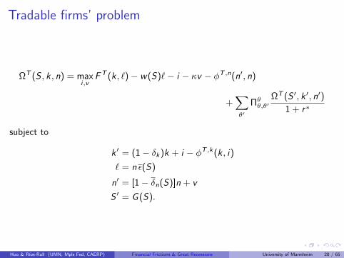
Tradable firms’ problem
ΩT (S , k, n) = maxi,v
FT (k, ℓ)− w(S)ℓ− i − κv − ϕT ,n(n′, n)
+∑θ′
Πθθ,θ′
ΩT (S ′, k ′, n′)
1 + r∗
subject to
k ′ = (1− δk)k + i − ϕT ,k(k, i)
ℓ = n ϵ(S)
n′ = [1− δn(S)]n + v
S ′ = G (S).
Huo & Rıos-Rull (UMN, Mpls Fed, CAERP) Financial Frictions & Great Recessions University of Mannheim 20 / 65

.....................
,..........
.....
.
Mutual fund
Financial wealth in the economy is
L+ =
∫b>0
b(S , ϵ, e, a) dx
Mortgages in the economy are
L− =
∫b<0
−b(S , ϵ, e, a) dx
Net foreign asset position of the country (the mutual fund owns all firms)
B = L+ −(ΩN(S)− πN(S) + ΩT (S)− πT (S) +
1
1 + r∗L−
)The realized rate of return is
1 + r(S ,S ′) =ΩN(S ′) + ΩT (S ′) + (1 + r∗)B + L−
L+
Huo & Rıos-Rull (UMN, Mpls Fed, CAERP) Financial Frictions & Great Recessions University of Mannheim 21 / 65

.....................
,..........
.....
.
Equilibrium
An equilibrium is a set of decision rules and values for households, firms’ valuesand decision rules, and a set aggregate variables of aggregate states, such that:
Households’ and firms’ policy functions and value functions solve thecorresponding program problems.
Aggregate searching consistence
D(S) =
∫d(S , x) dx ,
Nontradable prices satisfies
p(S) = pi (S ,KN ,NN) dx ,
Housing market clears ∫h(S , x) dx = H.
Huo & Rıos-Rull (UMN, Mpls Fed, CAERP) Financial Frictions & Great Recessions University of Mannheim 22 / 65

.....................
,..........
.....
.
Equilibrium
Average separation probability and labor force quality
δn(S) =
∑ϵ δn(ϵ)n(ϵ)
N, ϵ(S) =
∑ϵ ϵn(ϵ)
N
Rate of return to the mutual fund satisfies
1 + r(S , S ′) =ΩN(S ′) + ΩT (S ′) + (1 + r∗)B +
∫b<0
b(S , x)∫b>0
b(S , x)
Wage satisfieslogw(S)− logw = εw
(logY (S)− logY
)The law of motion G (S) is consistent with households’ decisions andemployment dynamics.
Huo & Rıos-Rull (UMN, Mpls Fed, CAERP) Financial Frictions & Great Recessions University of Mannheim 23 / 65

.....................
,..........
.....
.
Mapping the Model to Data
Huo & Rıos-Rull (UMN, Mpls Fed, CAERP) Financial Frictions & Great Recessions University of Mannheim 24 / 65

.....................
,..........
.....
.
Functional forms
Preferences
u(cA, h, d) =1
1− σc
(cA − ξd
d1+γ
1 + γ
)1−σc
+ v(h)
where there is an Armington aggregator for consumption
cA =
[ω (cNI
ρN)
η−1η + (1− ω)c
η−1η
T
] ηη−1
and houses are inferior goods.
v(h) =
ξh
1−σ1h(h + h1)
1−σ1h , if h < h
ξh1−σ2
h(h + h2)
1−σ2h , if h ≥ h.
Huo & Rıos-Rull (UMN, Mpls Fed, CAERP) Financial Frictions & Great Recessions University of Mannheim 25 / 65

.....................
,..........
.....
.
1 2 3 4 5−0.5
−0.45
−0.4
−0.35
−0.3
−0.25
−0.2
−0.15
−0.1
Housing function with less curvatureHousing function with more curvature
0 0.5 1 1.5 20
0.5
1
1.5
2
2.5
3
3.5
Housing
Consumption
Housing utility function Policy function: consumption vs housing
Huo & Rıos-Rull (UMN, Mpls Fed, CAERP) Financial Frictions & Great Recessions University of Mannheim 26 / 65

.....................
,..........
.....
.
Functional forms
Production function
FN(k , ℓ1, ℓ2) = zN kα0 ℓα11 ℓα2
2 , FT (k, ℓ) = zTkθ0ℓθ1
Capital adjustment cost in the nontradable goods sector
ϕN(i , k) =εN
2
(i
k− δk
)2
k
Capital and employment adjustment cost in the tradable goods sector
ϕT ,k(i , k) =εT ,k
2
(i
k− δk
)2
k, ϕT ,n(n′, n) =εT ,n
2
(n′
n− 1
)2
n
Matching technology
M(D,T ) = νDµT 1−µ
Huo & Rıos-Rull (UMN, Mpls Fed, CAERP) Financial Frictions & Great Recessions University of Mannheim 27 / 65

.....................
,..........
.....
.
Exogenously determined parameters
A period is half a quarter.
Parameter Value
Risk aversion for consumption, σc 2.0
Risk aversion for housing, σ1c 2.0
Risk aversion for housing, σ2c 10.0
Curvature of shopping, γ 2.0
Elasticity of substitution bw tradables and nontradables, η 0.80
Cutoff value for housing utility, h 2.0
Price markup, ρ 1.1
Loan to value ratio, λ 0.85
Interest rate for international bonds, r∗ 4%
Huo & Rıos-Rull (UMN, Mpls Fed, CAERP) Financial Frictions & Great Recessions University of Mannheim 28 / 65
.....................
,..........
.....
.
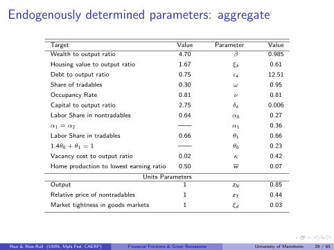
Endogenously determined parameters: aggregate
Target Value Parameter Value
Wealth to output ratio 4.70 β 0.985
Housing value to output ratio 1.67 ξh 0.61
Debt to output ratio 0.75 ϵ4 12.51
Share of tradables 0.30 ω 0.95
Occupancy Rate 0.81 ν 0.81
Capital to output ratio 2.75 δk 0.006
Labor Share in nontradables 0.64 α0 0.27
α1 = α2 —— α1 0.36
Labor Share in tradables 0.66 θ1 0.66
1.4θ0 + θ1 = 1 —— θ0 0.23
Vacancy cost to output ratio 0.02 κ 0.42
Home production to lowest earning ratio 0.50 w 0.07
Units ParametersOutput 1 zN 0.85
Relative price of nontradables 1 zT 0.44
Market tightness in goods markets 1 ξd 0.03
Huo & Rıos-Rull (UMN, Mpls Fed, CAERP) Financial Frictions & Great Recessions University of Mannheim 29 / 65

.....................
,..........
.....
.
Endogenously determined parameters: cross-section
Target Value Parameter Value
Job duration for type 1 1.5 year δ1n 0.083
Job duration for type 3 5 year δ3n 0.025
Job duration for type 4 5 year δ4n 0.025
Unemployment rate 6% δ2n 0.047
Wealth Gini index 0.82 Πϵ1,4 0.0003
Earning Gini index 0.64 Πϵ4,1 0.0031
Earning autocorrelation 0.95 Πϵ1,1 0.9894
Earning stdev 0.12 Πϵ2,2 0.9860
Transition matrix ϵ1 ϵ2 ϵ3 ϵ4
ϵ1 0.9894 0.0101 0.0000 0.0003
ϵ2 0.0067 0.9860 0.0067 0.0003
ϵ3 0.0000 0.0101 0.9894 0.0003
ϵ4 0.0031 0.0031 0.0031 0.9904
Skill Value 0.2259 0.4496 0.8948 12.50
Huo & Rıos-Rull (UMN, Mpls Fed, CAERP) Financial Frictions & Great Recessions University of Mannheim 30 / 65
.....................
,..........
.....
.
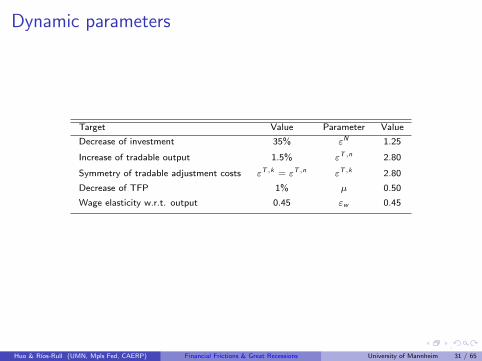
Dynamic parameters
Target Value Parameter Value
Decrease of investment 35% εN 1.25
Increase of tradable output 1.5% εT,n 2.80
Symmetry of tradable adjustment costs εT,k = εT,n εT,k 2.80
Decrease of TFP 1% µ 0.50
Wage elasticity w.r.t. output 0.45 εw 0.45
Huo & Rıos-Rull (UMN, Mpls Fed, CAERP) Financial Frictions & Great Recessions University of Mannheim 31 / 65

.....................
,..........
.....
.
Experiments: Financial Shocks
Huo & Rıos-Rull (UMN, Mpls Fed, CAERP) Financial Frictions & Great Recessions University of Mannheim 32 / 65

.....................
,..........
.....
.
Experiments
...1 Decrease the loan to value ratio from 0.85 to 0.75 in period 1, with flexible andfixed wage.
...2 Decrease the loan to value ratio from 0.85 to 0.75 gradually in 4 years, withflexible and fixed wage.
...3 Increase the interest rate for borrowing from 4% to 4.3% in period 1, withflexible and fixed wage.
...4 increase the interest rate for borrowing from 4% to 4.3% gradually in 4 years,with flexible and fixed wage.
...5 increase both the loan to value ratio from 0.85 to 0.75, and the interest ratefor borrowing from 4% to 4.3% gradually in 4 years, with flexible wage.
Huo & Rıos-Rull (UMN, Mpls Fed, CAERP) Financial Frictions & Great Recessions University of Mannheim 33 / 65

.....................
,..........
.....
.
1: Sudden change of λ. Flex. w Fixed w
0 1 2 3 4 5 6 7 8 9 10−3.5
−3
−2.5
−2
−1.5
−1
−0.5
0
0.5
Real output
0 1 2 3 4 5 6 7 8 9 105
6
7
8
9
10
11
Unemployment
0 1 2 3 4 5 6 7 8 9 10−5
−4
−3
−2
−1
0
1
Consumption
0 1 2 3 4 5 6 7 8 9 10−35
−30
−25
−20
−15
−10
−5
0
5
Investment
Huo & Rıos-Rull (UMN, Mpls Fed, CAERP) Financial Frictions & Great Recessions University of Mannheim 34 / 65

.....................
,..........
.....
.
1 Sudden change of λ, Flex. w Fixed w
0 1 2 3 4 5 6 7 8 9 10−3.5
−3
−2.5
−2
−1.5
−1
−0.5
0
0.5
Wealth
0 1 2 3 4 5 6 7 8 9 10−14
−12
−10
−8
−6
−4
−2
0
Debt
0 1 2 3 4 5 6 7 8 9 10−9
−8
−7
−6
−5
−4
−3
−2
−1
0
Housing price
Huo & Rıos-Rull (UMN, Mpls Fed, CAERP) Financial Frictions & Great Recessions University of Mannheim 35 / 65

.....................
,..........
.....
.
1. Sudden change of λ, Flex. w Fixed w
0 1 2 3 4 5 6 7 8 9 10−1
−0.8
−0.6
−0.4
−0.2
0
0.2
0.4
TFP with total hours
0 1 2 3 4 5 6 7 8 9 10−1
−0.5
0
0.5
1
1.5
Labor Productivity
0 1 2 3 4 5 6 7 8 9 10−0.2
0
0.2
0.4
0.6
0.8
1
1.2
1.4
1.6
Labor quality
0 1 2 3 4 5 6 7 8 9 10−1.2
−1
−0.8
−0.6
−0.4
−0.2
0
0.2
TFP with total labor inputs
Huo & Rıos-Rull (UMN, Mpls Fed, CAERP) Financial Frictions & Great Recessions University of Mannheim 36 / 65
.....................
,..........
.....
.
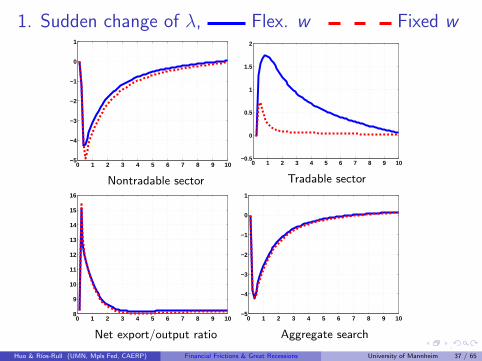
1. Sudden change of λ, Flex. w Fixed w
0 1 2 3 4 5 6 7 8 9 10−5
−4
−3
−2
−1
0
1
Nontradable sector
0 1 2 3 4 5 6 7 8 9 10−0.5
0
0.5
1
1.5
2
Tradable sector
0 1 2 3 4 5 6 7 8 9 108
9
10
11
12
13
14
15
16
Net export/output ratio
0 1 2 3 4 5 6 7 8 9 10−5
−4
−3
−2
−1
0
1
Aggregate search
Huo & Rıos-Rull (UMN, Mpls Fed, CAERP) Financial Frictions & Great Recessions University of Mannheim 37 / 65
.....................
,..........
.....
.
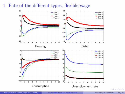
1. Fate of the different types, flexible wage
0 1 2 3 4 5 6 7 8 9 10−15
−10
−5
0
5
10
15
Type 1Type 2Type 3Type 4
Housing
0 1 2 3 4 5 6 7 8 9 10−40
−30
−20
−10
0
10
20
30
Type 1Type 2Type 3Type 4
Debt
0 1 2 3 4 5 6 7 8 9 10−10
−8
−6
−4
−2
0
2
4
Type 1Type 2Type 3Type 4
Consumption
0 1 2 3 4 5 6 7 8 9 102
4
6
8
10
12
14
16
Type 1Type 2Type 3Type 4
Unemployment rate
Huo & Rıos-Rull (UMN, Mpls Fed, CAERP) Financial Frictions & Great Recessions University of Mannheim 38 / 65

.....................
,..........
.....
.
2, slow change of λ Flex. w Fixed w
0 1 2 3 4 5 6 7 8 9 10−2.5
−2
−1.5
−1
−0.5
0
0.5
Real output
0 1 2 3 4 5 6 7 8 9 105.5
6
6.5
7
7.5
8
8.5
9
9.5
Unemployment
0 1 2 3 4 5 6 7 8 9 10−4
−3.5
−3
−2.5
−2
−1.5
−1
−0.5
0
0.5
Consumption
0 1 2 3 4 5 6 7 8 9 10−25
−20
−15
−10
−5
0
5
Investment
Huo & Rıos-Rull (UMN, Mpls Fed, CAERP) Financial Frictions & Great Recessions University of Mannheim 39 / 65

.....................
,..........
.....
.
2, slow change of λ Flex. w Fixed w
0 1 2 3 4 5 6 7 8 9 10−3
−2.5
−2
−1.5
−1
−0.5
0
0.5
Wealth
0 1 2 3 4 5 6 7 8 9 10−10
−8
−6
−4
−2
0
Debt
0 1 2 3 4 5 6 7 8 9 10−7
−6
−5
−4
−3
−2
−1
0
Housing price
Huo & Rıos-Rull (UMN, Mpls Fed, CAERP) Financial Frictions & Great Recessions University of Mannheim 40 / 65
.....................
,..........
.....
.
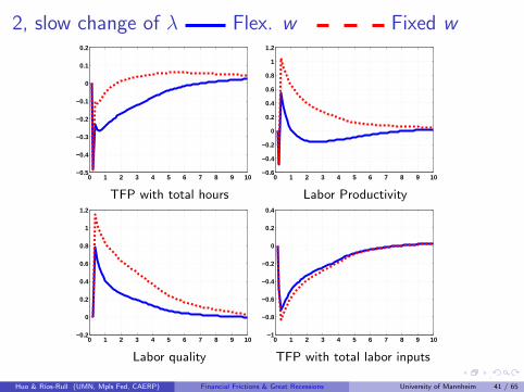
2, slow change of λ Flex. w Fixed w
0 1 2 3 4 5 6 7 8 9 10−0.5
−0.4
−0.3
−0.2
−0.1
0
0.1
0.2
TFP with total hours
0 1 2 3 4 5 6 7 8 9 10−0.6
−0.4
−0.2
0
0.2
0.4
0.6
0.8
1
1.2
Labor Productivity
0 1 2 3 4 5 6 7 8 9 10−0.2
0
0.2
0.4
0.6
0.8
1
1.2
Labor quality
0 1 2 3 4 5 6 7 8 9 10−1
−0.8
−0.6
−0.4
−0.2
0
0.2
0.4
TFP with total labor inputs
Huo & Rıos-Rull (UMN, Mpls Fed, CAERP) Financial Frictions & Great Recessions University of Mannheim 41 / 65

.....................
,..........
.....
.
3. Sudden ∆ς , Flex. w Fixed w
0 1 2 3 4 5 6 7 8 9 10−2.5
−2
−1.5
−1
−0.5
0
Real output
0 1 2 3 4 5 6 7 8 9 106
6.5
7
7.5
8
8.5
9
9.5
Unemployment
0 1 2 3 4 5 6 7 8 9 10−4
−3.5
−3
−2.5
−2
−1.5
−1
−0.5
0
Consumption
0 1 2 3 4 5 6 7 8 9 10−30
−25
−20
−15
−10
−5
0
5
Investment
Huo & Rıos-Rull (UMN, Mpls Fed, CAERP) Financial Frictions & Great Recessions University of Mannheim 42 / 65

.....................
,..........
.....
.
3. Sudden ∆ς , Flex. w Fixed w
0 1 2 3 4 5 6 7 8 9 10−3.5
−3
−2.5
−2
−1.5
−1
−0.5
0
Wealth
0 1 2 3 4 5 6 7 8 9 10−8
−7
−6
−5
−4
−3
−2
−1
0
Debt
0 1 2 3 4 5 6 7 8 9 10−9
−8
−7
−6
−5
−4
−3
−2
−1
0
Housing price
Huo & Rıos-Rull (UMN, Mpls Fed, CAERP) Financial Frictions & Great Recessions University of Mannheim 43 / 65

.....................
,..........
.....
.
3. Sudden ∆ς , Flex. w Fixed w
0 1 2 3 4 5 6 7 8 9 10−0.6
−0.5
−0.4
−0.3
−0.2
−0.1
0
0.1
TFP with total hours
0 1 2 3 4 5 6 7 8 9 10−0.6
−0.4
−0.2
0
0.2
0.4
0.6
0.8
1
1.2
Labor Productivity
0 1 2 3 4 5 6 7 8 9 100
0.2
0.4
0.6
0.8
1
1.2
1.4
Labor quality
0 1 2 3 4 5 6 7 8 9 10−0.9
−0.8
−0.7
−0.6
−0.5
−0.4
−0.3
−0.2
−0.1
0
TFP with total labor inputs
Huo & Rıos-Rull (UMN, Mpls Fed, CAERP) Financial Frictions & Great Recessions University of Mannheim 44 / 65

.....................
,..........
.....
.
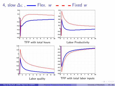
4, Slow ∆ς , Flex. w Fixed w
0 1 2 3 4 5 6 7 8 9 10−2.5
−2
−1.5
−1
−0.5
0
Real output
0 1 2 3 4 5 6 7 8 9 106
6.5
7
7.5
8
8.5
9
9.5
Unemployment
0 1 2 3 4 5 6 7 8 9 10−4
−3.5
−3
−2.5
−2
−1.5
−1
−0.5
0
Consumption
0 1 2 3 4 5 6 7 8 9 10−25
−20
−15
−10
−5
0
5
Investment
Huo & Rıos-Rull (UMN, Mpls Fed, CAERP) Financial Frictions & Great Recessions University of Mannheim 45 / 65
.....................
,..........
.....
.
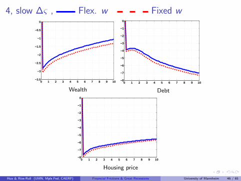
4, slow ∆ς , Flex. w Fixed w
0 1 2 3 4 5 6 7 8 9 10−3.5
−3
−2.5
−2
−1.5
−1
−0.5
0
Wealth
0 1 2 3 4 5 6 7 8 9 10−8
−7
−6
−5
−4
−3
−2
−1
0
Debt
0 1 2 3 4 5 6 7 8 9 10−8
−7
−6
−5
−4
−3
−2
−1
0
Housing price
Huo & Rıos-Rull (UMN, Mpls Fed, CAERP) Financial Frictions & Great Recessions University of Mannheim 46 / 65
.....................
,..........
.....
.
4, slow ∆ς , Flex. w Fixed w
0 1 2 3 4 5 6 7 8 9 10−0.5
−0.4
−0.3
−0.2
−0.1
0
0.1
0.2
TFP with total hours
0 1 2 3 4 5 6 7 8 9 10−0.6
−0.4
−0.2
0
0.2
0.4
0.6
0.8
1
1.2
Labor Productivity
0 1 2 3 4 5 6 7 8 9 100
0.2
0.4
0.6
0.8
1
1.2
1.4
Labor quality
0 1 2 3 4 5 6 7 8 9 10−0.9
−0.8
−0.7
−0.6
−0.5
−0.4
−0.3
−0.2
−0.1
0
TFP with total labor inputs
Huo & Rıos-Rull (UMN, Mpls Fed, CAERP) Financial Frictions & Great Recessions University of Mannheim 47 / 65

.....................
,..........
.....
.
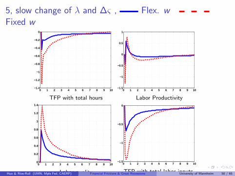
5, slow change of λ and ∆ς , Flex. wFixed w
0 1 2 3 4 5 6 7 8 9 10−3.5
−3
−2.5
−2
−1.5
−1
−0.5
0
Real output
0 1 2 3 4 5 6 7 8 9 106
6.5
7
7.5
8
8.5
9
9.5
10
Unemployment
0 1 2 3 4 5 6 7 8 9 10−6
−5
−4
−3
−2
−1
0
Consumption
0 1 2 3 4 5 6 7 8 9 10−50
−40
−30
−20
−10
0
10
Investment
Slow change λ Slow change of λ and borrowing cost
Huo & Rıos-Rull (UMN, Mpls Fed, CAERP) Financial Frictions & Great Recessions University of Mannheim 48 / 65

.....................
,..........
.....
.
5, slow change of λ and ∆ς , Flex. wFixed w
0 1 2 3 4 5 6 7 8 9 10−5
−4
−3
−2
−1
0
Wealth
0 1 2 3 4 5 6 7 8 9 10−16
−14
−12
−10
−8
−6
−4
−2
0
Debt
0 1 2 3 4 5 6 7 8 9 10−14
−12
−10
−8
−6
−4
−2
0
Housing price
Slow change λ Slow change of λ and borrowing cost
Huo & Rıos-Rull (UMN, Mpls Fed, CAERP) Financial Frictions & Great Recessions University of Mannheim 49 / 65
.....................
,..........
.....
.
5, slow change of λ and ∆ς , Flex. wFixed w
0 1 2 3 4 5 6 7 8 9 10−1.4
−1.2
−1
−0.8
−0.6
−0.4
−0.2
0
TFP with total hours
0 1 2 3 4 5 6 7 8 9 10−1.5
−1
−0.5
0
0.5
1
Labor Productivity
0 1 2 3 4 5 6 7 8 9 100
0.2
0.4
0.6
0.8
1
1.2
1.4
Labor quality
0 1 2 3 4 5 6 7 8 9 10−1.5
−1
−0.5
0
TFP with total labor inputs
Slow change λ Slow change of λ and borrowing cost
Huo & Rıos-Rull (UMN, Mpls Fed, CAERP) Financial Frictions & Great Recessions University of Mannheim 50 / 65

.....................
,..........
.....
.
Results: larger TFP drop? Sudden change of λ withµ = 0.8
0 1 2 3 4 5 6 7 8 9 10−1.6
−1.4
−1.2
−1
−0.8
−0.6
−0.4
−0.2
0
0.2
TFP with total hours
0 1 2 3 4 5 6 7 8 9 10−1.5
−1
−0.5
0
0.5
1
Labor Productivity
0 1 2 3 4 5 6 7 8 9 10−0.2
0
0.2
0.4
0.6
0.8
1
1.2
Labor quality
0 1 2 3 4 5 6 7 8 9 10−2
−1.5
−1
−0.5
0
0.5
TFP with total labor inputs
Baseline, flexible wage Higher µ, flexible wage
Huo & Rıos-Rull (UMN, Mpls Fed, CAERP) Financial Frictions & Great Recessions University of Mannheim 51 / 65

.....................
,..........
.....
.
Model properties
All the experiments generate
Drop of output, employment, investment and consumption.
Drop of wealth, housing price and debt.
Drop of total productivity, increase of labor quality and labor productivity.
With fixed wage, the recovery of employment is much slower.
With slow change of the financial condition, the initial drop of debt is smaller,which is the case in the data.
A decrease of the loan to value ratio λ and an increase of borrowing cost havesimilar effects.
Huo & Rıos-Rull (UMN, Mpls Fed, CAERP) Financial Frictions & Great Recessions University of Mannheim 52 / 65

.....................
,..........
.....
.
Results: an expansion? Change λ from 0.75 to 0.85
0 1 2 3 4 5 6 7 8 9 100
0.2
0.4
0.6
0.8
1
1.2
1.4
Real output
0 1 2 3 4 5 6 7 8 9 104
4.2
4.4
4.6
4.8
5
5.2
5.4
5.6
5.8
Unemployment
0 1 2 3 4 5 6 7 8 9 100
0.5
1
1.5
2
2.5
Consumption
0 1 2 3 4 5 6 7 8 9 10−5
0
5
10
15
20
Investment
Sudden change of λ Slow change of λHuo & Rıos-Rull (UMN, Mpls Fed, CAERP) Financial Frictions & Great Recessions University of Mannheim 53 / 65
.....................
,..........
.....
.
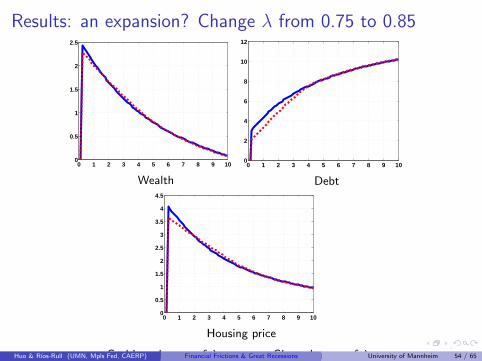
Results: an expansion? Change λ from 0.75 to 0.85
0 1 2 3 4 5 6 7 8 9 100
0.5
1
1.5
2
2.5
Wealth
0 1 2 3 4 5 6 7 8 9 100
2
4
6
8
10
12
Debt
0 1 2 3 4 5 6 7 8 9 100
0.5
1
1.5
2
2.5
3
3.5
4
4.5
Housing price
Sudden change of λ Slow change of λHuo & Rıos-Rull (UMN, Mpls Fed, CAERP) Financial Frictions & Great Recessions University of Mannheim 54 / 65

.....................
,..........
.....
.
Results: an expansion? Change λ from 0.75 to 0.85
0 1 2 3 4 5 6 7 8 9 10−0.05
0
0.05
0.1
0.15
0.2
0.25
0.3
0.35
TFP with total hours
0 1 2 3 4 5 6 7 8 9 10−0.5
−0.4
−0.3
−0.2
−0.1
0
0.1
0.2
0.3
0.4
Labor Productivity
0 1 2 3 4 5 6 7 8 9 10−0.7
−0.6
−0.5
−0.4
−0.3
−0.2
−0.1
0
Labor quality
0 1 2 3 4 5 6 7 8 9 100
0.1
0.2
0.3
0.4
0.5
0.6
0.7
TFP with total labor inputs
Sudden change of λ Slow change of λHuo & Rıos-Rull (UMN, Mpls Fed, CAERP) Financial Frictions & Great Recessions University of Mannheim 55 / 65
.....................
,..........
.....
.
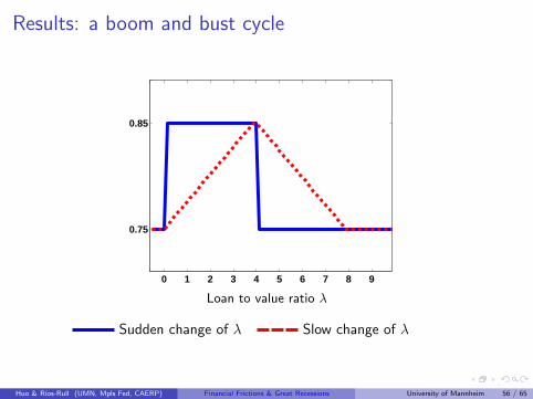
Results: a boom and bust cycle
0 1 2 3 4 5 6 7 8 9
0.75
0.85
Loan to value ratio λ
Sudden change of λ Slow change of λ
Huo & Rıos-Rull (UMN, Mpls Fed, CAERP) Financial Frictions & Great Recessions University of Mannheim 56 / 65

.....................
,..........
.....
.
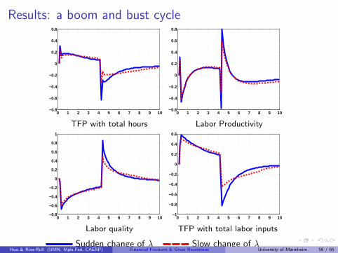
Results: a boom and bust cycle
0 1 2 3 4 5 6 7 8 9 10−2
−1.5
−1
−0.5
0
0.5
1
1.5
Real output
0 1 2 3 4 5 6 7 8 9 104
4.5
5
5.5
6
6.5
7
7.5
8
8.5
Unemployment
0 1 2 3 4 5 6 7 8 9 10−3
−2
−1
0
1
2
3
Consumption
0 1 2 3 4 5 6 7 8 9 10−30
−20
−10
0
10
20
Investment
Sudden change of λ Slow change of λHuo & Rıos-Rull (UMN, Mpls Fed, CAERP) Financial Frictions & Great Recessions University of Mannheim 57 / 65

.....................
,..........
.....
.
Results: a boom and bust cycle
0 1 2 3 4 5 6 7 8 9 10−2
−1.5
−1
−0.5
0
0.5
1
1.5
2
2.5
Wealth0 1 2 3 4 5 6 7 8 9 10
0
1
2
3
4
5
6
7
8
Debt
0 1 2 3 4 5 6 7 8 9 10−6
−4
−2
0
2
4
6
Housing price
Sudden change of λ Slow change of λHuo & Rıos-Rull (UMN, Mpls Fed, CAERP) Financial Frictions & Great Recessions University of Mannheim 58 / 65
.....................
,..........
.....
.
Results: a boom and bust cycle
0 1 2 3 4 5 6 7 8 9 10−0.8
−0.6
−0.4
−0.2
0
0.2
0.4
0.6
TFP with total hours
0 1 2 3 4 5 6 7 8 9 10−0.6
−0.4
−0.2
0
0.2
0.4
0.6
0.8
Labor Productivity
0 1 2 3 4 5 6 7 8 9 10−0.8
−0.6
−0.4
−0.2
0
0.2
0.4
0.6
0.8
1
Labor quality
0 1 2 3 4 5 6 7 8 9 10−1
−0.8
−0.6
−0.4
−0.2
0
0.2
0.4
0.6
TFP with total labor inputs
Sudden change of λ Slow change of λHuo & Rıos-Rull (UMN, Mpls Fed, CAERP) Financial Frictions & Great Recessions University of Mannheim 59 / 65

.....................
,..........
.....
.
Model properties
All the experiments generate
Drop of output, employment, investment and consumption.
Drop of wealth, housing price and debt.
Drop of total productivity, increase of labor quality and labor productivity.
With fixed wage, the initial drop of employment is larger and the recovery ismuch slower.
With slow change of the financial condition, the initial drop of debt is smaller,which is the case in the data.
A decrease of the loan to value ratio λ and an increase of borrowing cost havesimilar effects.
Huo & Rıos-Rull (UMN, Mpls Fed, CAERP) Financial Frictions & Great Recessions University of Mannheim 60 / 65
.....................
,..........
.....
.
Insufficient drop of housing price
In the data: housing price ↓ 20%, housing value ↓ 36%.
In the model: housing price ↓ 6% to 14%.
Problem:
Rich households with deep pockets pick up the slack. Not so much in the realworld.
Large decline of housing price may force poor households default their debt.Not allowed in the model.
Solution:
Housing utility function with more curvature.
Smaller initial load to value ratio λ gives larger room for drop of housing pricewithout default.
Huo & Rıos-Rull (UMN, Mpls Fed, CAERP) Financial Frictions & Great Recessions University of Mannheim 61 / 65

.....................
,..........
.....
.
Housing utility function
A three-piece housing utility function.
1.5 2 2.5 3 3.5
A
B C
A: greater curvature to prevent rich households from expanding houses.
B: greater curvature to prevent super rich households from expanding houses.
C: upper bound for housing holding.
Huo & Rıos-Rull (UMN, Mpls Fed, CAERP) Financial Frictions & Great Recessions University of Mannheim 62 / 65

.....................
,..........
.....
.
Housing as a function of consumption.
0.2 0.3 0.4 0.5 0.6 0.7
Consumption
Rich households will not increase their housing by much due to decreasingmarginal utility.
Housing price has to drop more to induce poor households not to sell theirhouses.
Huo & Rıos-Rull (UMN, Mpls Fed, CAERP) Financial Frictions & Great Recessions University of Mannheim 63 / 65
.....................
,..........
.....
.
Conclusions
We have a recession generated purely by increased difficulties to borrow on thepart of households
The recession comes together with TFP loses
Drop in Housing prices (movements too sharp because of lack of house frictions)
Drop in Stock Market
Still insufficient drop in asset prices
The literature is trying hard to get this (Midrigan and Philippon (2011), Guerrieri and
Lorenzoni (2009)) with limited success.
Still ways to go.
Huo & Rıos-Rull (UMN, Mpls Fed, CAERP) Financial Frictions & Great Recessions University of Mannheim 64 / 65
.....................
,..........
.....
.
References
Fang, Lei and Jun Nie. 2013. “Education, Human Capital and U.S. Labor Market Dynamics.” Presented at MidWest Macro Meetings.
Gornemann, Nils, Keith Kuester, and Makoto Nakajima. 2012. “Monetary Policy with Heterogeneous Agents.” Mimeo, FRB Philadelphia.
Guerrieri, Veronica and Guido Lorenzoni. 2009. “Liquidity and Trading Dynamics.” Econometrica 77 (6):1751–1790.
Midrigan, V. and T. Philippon. 2011. “Household Leverage and the Recession.” NYU Working Paper FIN-11-038, New York University.
Huo & Rıos-Rull (UMN, Mpls Fed, CAERP) Financial Frictions & Great Recessions University of Mannheim 65 / 65


![INDEX [] · Human development Index ... Giffin Goods = When prices goes up demand of Inferior goods increases. 4. ... - During the recession, ...](https://static.fdocuments.net/doc/165x107/5b5aef8f7f8b9ab8578d016e/index-human-development-index-giffin-goods-when-prices-goes-up-demand.jpg)