The Ronald O. Perelman Center for Political Science and Economics (PCPSE) 133 South 36th Street Philadelphia, PA 19104-6297

pier@econ.upenn.edu http://economics.sas.upenn.edu/pier

PIER Working Paper

19-015

Financial Frictions and the

Wealth Distribution

JESÚS FERNÁNDEZ-VILLAVERDE University of Pennsylvania, NBER, and CEPR

SAMUEL HURTADO GALO NUÑO Banco de España Banco de España

September 13, 2019

https://ssrn.com/abstract=3455286

Financial Frictions and the Wealth Distribution

Jesus Fernandez-Villaverde

University of Pennsylvania, NBER, and CEPR

Samuel Hurtado Galo Nuno

Banco de Espana Banco de Espana∗

September 13, 2019

Abstract

This paper investigates how, in a heterogeneous agents model with financial frictions,

idiosyncratic individual shocks interact with exogenous aggregate shocks to generate time-

varying levels of leverage and endogenous aggregate risk. To do so, we show how such a

model can be efficiently computed, despite its substantial nonlinearities, using tools from

machine learning. We also illustrate how the model can be structurally estimated with

a likelihood function, using tools from inference with diffusions. We document, first, the

strong nonlinearities created by financial frictions. Second, we report the existence of

multiple stochastic steady states with properties that differ from the deterministic steady

state along important dimensions. Third, we illustrate how the generalized impulse re-

sponse functions of the model are highly state-dependent. In particular, we find that the

recovery after a negative aggregate shock is more sluggish when the economy is more lever-

aged. Fourth, we prove that wealth heterogeneity matters in this economy because of the

asymmetric responses of household consumption decisions to aggregate shocks.

Keywords: Heterogeneous agents; aggregate shocks; continuous-time; machine learning;

neural networks; structural estimation; likelihood functions.

JEL codes: C45, C63, E32, E44, G01, G11.

∗We thank Manuel Arellano, Emmanuel Farhi, Xavier Gabaix, Lars Peter Hansen, Mark Gertler, DavideMelcangi, Ben Moll, Gianluca Violante, Ivan Werning, and participants at numerous seminars and conferencesfor pointed comments. The views expressed in this manuscript are those of the authors and do not necessarilyrepresent the views of the Eurosystem or the Bank of Spain.

1

1 Introduction

How do financial frictions interact with households’ wealth heterogeneity to shape aggregate

dynamics? In this paper we investigate how, in a heterogeneous agents model with financial

frictions, idiosyncratic individual shocks interact with exogenous aggregate shocks to generate

time-varying levels of leverage and endogenous aggregate risk. Such an economy displays highly

nonlinear behavior, with i) multiple stochastic steady states; ii) multimodal and skewed er-

godic distributions of endogenous variables; and iii) strong state-dependence on the responses

of endogenous variables to aggregate shocks.

To do so, we build, compute, and estimate using the likelihood approach a continuous-time

neoclassical growth model with heterogeneous households subject to labor productivity shocks.

We enrich the model with a financial expert (a stand-in for banks or financial intermediaries),

limited financial markets participation and an aggregate shock to physical capital. Households

save in a noncontingent bond to self-insure against their labor productivity shocks and the vari-

ations in income induced by aggregate risk. The financial expert cannot issue state-contingent

assets (i.e., outside equity), but it can issue bonds to leverage its equity and accumulate capital

that is rented to a representative firm. Only the expert can hold capital.

The interaction between the demand for bonds by the households and the supply of bonds by

the financial expert begets, for parameter values that match important aspects of the U.S. data

and maximize the likelihood function, multiple stochastic steady states (SSSs). This multiplicity

occurs even despite the model having a unique deterministic steady state (DSS).1 In particular,

we will have a high-leverage SSS (HL-SSS) and a low-leverage SSS (LL-SSS), each with its basin

of attraction and endogenous level of aggregate risk (there is a third, unstable SSS that we do

not need to discuss).

The intuition for the existence of multiple stable SSSs is as follows. In the basin of attraction

of the HL-SSS, a negative aggregate shock to capital has dire effects. The financial expert’s net

wealth is greatly eroded, since her relatively small equity must absorb all the losses to capital.

The economy suffers a deep and prolonged recession as the expert struggles to rebuild her

equity and accumulate capital. This recession translates into persistently low wages. Since the

households want to self-insure against the risk of low wages, their demand for bonds is high:

this SSS has a higher share of wealthy households and more wealth and income inequality than

the DSS. The high demand for bonds translates into a low risk-free interest rate for the bond

and a high expected excess return for capital, which, in turn, induce the financial expert to lever

aggressively. A high-leverage region of the economy is a region with high aggregate volatility,

even when the variance of the aggregate shock is the same as in the low-leverage region.

1An SSS, also known as a risky steady state, is a fixed point of the equilibrium conditions of the model whenthe realization of the aggregate shock is zero. A DSS is a fixed point of the equilibrium conditions of the modelwhen the volatility of the aggregate shock (but not of idiosyncratic shocks) is zero.

2

In comparison, when the financial expert is lowly levered, the recessions after a negative

aggregate shock are mild. Thus, the demand for bonds by the household is low, the risk-

free rate high, the expected excess return low, and these prices sustain the low leverage by

the expert. With low leverage, the endogenous aggregate risk of the economy is smaller: the

economy responds more mutedly to the same aggregate shock than when leverage is high.

To show the higher persistence of shocks when leverage is high, we compute the general-

ized impulse response functions and the distributional impulse response functions to a negative

capital shock in different points of the state space. The responses are similar on impact, but

the ensuing recession is more persistent when leverage is high due to the dynamics of aggregate

household consumption and capital accumulation. In a high-leverage economy, the expected

path of interest rates is more persistent as the financial expert slowly restores her net wealth.

This persistence induces a less severe decline in consumption among wealthy households and

sluggish capital accumulation by the expert because the more persistent interest rates justify

less intertemporal substitution.

For our baseline parameter values, the economy will spend more time, on average, around

the HL-SSS than around the LL-SSS. We will show, however, how this finding varies as we

change the volatility of idiosyncratic and aggregate shocks.

The multiplicity of SSSs does not imply a multiplicity of equilibria: in our model, we find a

unique stochastic equilibrium. Whether the economy has high or low leverage is a consequence of

the past aggregate shocks. Sometimes, while the economy is traveling in the basin of attraction

of the HL-SSS, a sequence of aggregate shocks will move it to the basin of attraction of the LL-

SSS (and vice versa). Thus, the interaction of financial frictions with the consumption-saving

decisions made by the agents generates time variation in aggregate risk: after some sequences of

shocks, the economy will be fragile and prone to severe recessions due to high leverage and, after

other sequences, the economy will be more resilient and less volatile thanks to low leverage.

The argument above also explains why household heterogeneity is crucial for our argument

and why the “approximate aggregation result” of Krusell and Smith (1998) breaks down in our

environment. While the consumption decision rule of the households is close to linear with

respect to the household state variables (except for very poor households), it is not with respect

to the aggregate state variables.

A consequence of this breakdown of the “approximate aggregation result” is that, as we

reduce idiosyncratic labor productivity risk for a given volatility of the aggregate shock, the

model encounters a bifurcation and the HL-SSS disappears. The precautionary saving motive

becomes smaller and the households do not demand enough bonds to sustain the HL-SSS.

Conversely, when we increase the level of idiosyncratic labor productivity risk, the LL-SSS

disappears and only the HL-SSS survives. In this case, households are so concerned about

their own idiosyncratic labor risk that they demand enough bonds as to push the risk-free rate

3

sufficiently low that only a high level of leverage can be an SSS (paradoxically, increasing the

aggregate risk they face).

In practical terms, higher micro turbulence (e.g., more volatile labor markets) translates in

our model into higher aggregate volatility even when the variance of aggregate shocks is constant.

This result suggests that the rise in wealth inequality among capital owners documented by

Alvaredo et al. (2017) before the financial crisis of 2007 is linked with i) the increase in financial

debt and leverage witnessed during the same period (Adrian and Shin, 2010, and Nuno and

Thomas, 2017); ii) low risk-free interest rates (Holston et al., 2017); and iii) the heightened

fragility of the economy to adverse shocks.

This mechanism is, as far as we know, new in the literature. It is different from the “paradox

of volatility” in Brunnermeier and Sannikov (2014). In their model, a low volatility of aggre-

gate shocks leads to higher leverage by the financial expert and, thus, deep recessions when a

large shock hits the economy. In our model, a high volatility of idiosyncratic shocks leads to

higher leverage and, thus, larger recessions on average, even when the aggregate shocks are not

particularly large. The mechanism is also different from that in Kumhof et al. (2015) because,

in our model, the change in the wealth distribution is endogenous and not the consequence of

an exogenous shock to the income received by top earners.

The documentation of the importance of individual heterogeneity in models with financial

frictions is a novel contribution of our paper. The insight that, with financial frictions, the wealth

distribution is a state of the economy is not new. Bernanke et al. (1999) and Kiyotaki and Moore

(1997) already discussed the idea. However, the literature has focused on the case where there is

between-agents heterogeneity, but no within-agents heterogeneity. Between-agents heterogeneity

means that capital owners are different from experts. No within-agents heterogeneity means

there is just one capital owner (a representative household) and a representative expert (or,

perhaps, different capital owners and experts but where the heterogeneity is collapsed into an

economy-wide average of leverage). Our model illustrates why within-agents heterogeneity is

crucial to understanding the aggregate consequences of financial frictions.

Researchers have largely avoided studying economies with within-agents heterogeneity and

financial frictions because characterizing this class of models is challenging: since the wealth

distribution is an infinite-dimensional object, standard dynamic programming techniques cannot

be employed. To overcome this problem, our paper provides new tools for the global, nonlinear

solution and estimation of heterogeneous agent models with aggregate shocks.

More concretely, we rely on the machine learning literature and employ a neural network

to obtain a flexible approximation of the perceived law of motion (PLM) of the cross-sectional

distribution of assets (the expert’s equity and households’ bonds) with a finite set of moments

in the spirit of Krusell and Smith (1998). Naturally, other machine learning schemes may also

be proposed (or, for the matter, other nonlinear universal approximators such as series expan-

4

sions or splines). However, our approach is particularly convenient, both regarding theoretical

properties and practical considerations.

First, the universal approximation theorem (Hornik et al., 1989; Cybenko, 1989; Bach, 2017)

states that a neural network can approximate any unknown Borel measurable function. Second,

the neural network breaks the curse of dimensionality for a large class of approximated functions,

which allows our method to be extended to much richer environments with many state variables

(or more moments). Third, the neural network can be efficiently trained using a combination

of the gradient descent and the back-propagation algorithms. Fourth, not only is our algorithm

efficient and easy to code, but also particularly amenable to massive parallelization in GPUs,

FPGAs, and dedicated AI accelerators such as TPUs. Finally, our approach reflects in a fairly

transparent way the self-justified equilibria nature of the “bounded rationality” solution of most

heterogeneous agents models (Kubler and Scheidegger, 2018). The PLM is computed based on

the samples drawn in the simulation of paths within the aggregate ergodic distribution. The

agents employ the neural network to extrapolate the dynamics outside of the equilibrium region.

In comparison, in Krusell and Smith (1998) and most of the subsequent literature, the

PLM of the aggregate variables is approximately linear in the endogenous state variables (but

nonlinear in the exogenous states, since the coefficients of the regression are allowed to vary

across shocks). This traditional PLM is a poor choice in our model, in which the nonlinearities

of the endogenous state variables play a central role and where, because of the use of continuous

time, exogenous states are incorporated into the endogenous states instantaneously. In fact,

we will document how a naive implementation of the Krusell and Smith (1998) algorithm in

our economy, and even of refinements such as Chebyshev polynomials, deliver a much worse

numerical performance. Neural networks allow us to be much more flexible and to avoid having

to specify, ex-ante, any nonlinear structure of the PLM.

Continuous time helps us to characterize much of the equilibrium dynamics analytically and

to worry only about local derivatives (instead of the whole shape of equilibrium functions) even

when solving the model globally. However, nothing essential depends on this choice and we

could replicate our approach –with higher computational costs– in discrete time. Achdou et al.

(2017) and Nuno and Thomas (2016) provide a more general presentation of the advantages of

continuous-time methods.

We also illustrate how a fully nonlinear model can be structurally estimated with a likeli-

hood function with aggregate and micro observations using tools from inference with diffusions

(Lo, 1988). Such likelihood is computationally straightforward once we have solved the model

with the approach outlined above: it just amounts to transposing a matrix. In particular, it

avoids having to resort to more computationally intensive algorithms such as the particle fil-

ter (Fernandez-Villaverde and Rubio-Ramırez, 2007). Then, we take our model to the data

by matching some features of the U.S. economy, such as the average leverage of the corporate

5

sector, and estimating the volatility of the aggregate shocks by maximum likelihood.

Our work relates to several important threads in macroeconomics. First, we follow the macro-

finance literature pioneered by Basak and Cuoco (1998), Adrian and Boyarchenko (2012), He

and Krishnamurthy (2012, 2013), and Brunnermeier and Sannikov (2014), among others. As

we mentioned before, most of these papers only consider between-agents heterogeneity, but

no within-agents heterogeneity. Instead, we deal with a nontrivial wealth distribution across

households and show why such heterogeneity matters.

Our paper also contributes to the literature on global solution methods for heterogeneous

agents models with aggregate shocks such as Den Haan (1996, 1997), Algan et al. (2008), Reiter

(2009, 2010), Den Haan and Rendahl (2010), Maliar et al. (2010), Sager (2014), Prohl (2015),

Bayer and Luetticke (2018), and Auclert et al. (2019) (Algan et al. 2014 is a recent survey of

the field). To the best of our knowledge, ours is the first paper to generalize the celebrated

algorithm of Krusell and Smith (1998) to accommodate a universal nonlinear law of motion in

the endogenous state variables.2

Finally, our paper builds on the nascent literature on the application of machine learning

techniques to compute dynamic equilibrium models. The proposed methods have so far been

concerned with the solution of high-dimensional dynamic programming problems. Scheidegger

and Bilionis (2017) combine Gaussian process regression with an active subspace method to

solve discrete-time stochastic growth models of up to 500 dimensions. Duarte (2018) employs a

reinforcement learning algorithm together with a neural network to solve a two-sector model with

11 state variables. In contrast, our machine learning algorithm is used to provide a nonlinear

forecast of aggregate variables within the model. In this respect, our paper reconnects with

an early literature using neural networks to model bounded rationality and learning, such as

Barucci and Landi (1995), Cho (1995), Cho and Sargent (1996), and Salmon (1995).

Our methodology may also be useful to analyze other heterogeneous agents models with

aggregate shocks. An obvious candidate is the heterogeneous agent New Keynesian (HANK)

model with a zero lower bound (ZLB) on the nominal interest rates, such as Auclert (2016),

Auclert and Rognlie (2018), Gornemann et al. (2012), Kaplan et al. (2018), Luetticke (2015),

and McKay et al. (2016). The ZLB introduces a nonlinearity in the state space of aggregate

variables that cannot be addressed either with local methods or with global methods based on

linear laws of motion. Other potential candidates include any model that requires a solution

with nonlinear features to provide an accurate characterization of the equilibrium dynamics of

the agents’ distribution.

2Ahn et al. (2017) introduce a related method to compute the solution to heterogeneous agents models withaggregate shocks in continuous time. However, theirs is a local solution, based on first-order perturbation aroundthe DSS and, thus, unable to analyze the class of nonlinear phenomena posed by our paper.

6

2 Model

We postulate a continuous-time, infinite-horizon model. Three types of agents populate our

economy: a representative firm, a representative financial expert, and a continuum of households.

There are two assets: a risky asset, capital, and a risk-free one, noncontingent bonds. Only

the expert can hold the risky asset. In the interpretation implicit in our terminology, this is

because the expert is the only agent with knowledge in accumulating capital. However, other

interpretations, such as the expert standing in for banks or financial intermediaries, are possible.

In contrast, households can lend to the expert at the risk-free rate, but cannot hold capital

themselves, as they lack the required skill to handle it. The expert cannot issue outside equity,

but she can partially finance her holdings of the risky asset by issuing bonds to households.

Together with market clearing, our assumptions imply that, at the aggregate level, there is a

positive net supply of capital, while bonds are in zero net supply. As will become apparent below,

there is no need to separate between the firm and the expert, and we could write the model

consolidating both agents into a single type. Keeping both agents separate, though, clarifies

the exposition. We introduce heterogeneity on the side of the households –but not among

the experts or the firms– because this is the heterogeneity that generates the most interesting

aggregate outcomes in our environment.

2.1 The firm

A representative firm rents aggregate capital, Kt, and aggregate labor, Lt, to produce output

with a Cobb-Douglas technology Yt = F (Kt, Lt) = Kαt L

1−αt . Since input markets are competi-

tive, wages, wt, are equal to the marginal productivity of labor:

wt =∂F (Kt, Lt)

∂Lt= (1− α)

YtLt

(1)

and the rental rate of capital, rct, is equal to the marginal productivity of capital:

rct =∂F (Kt, Lt)

∂Kt

= αYtKt

. (2)

During production, capital depreciates at a constant rate δ and receives a growth rate shock

Zt that follows a Brownian motion with volatility σ. Thus, aggregate capital evolves as:

dKt

Kt

= (ιt − δ) dt+ σdZt, (3)

where ιt is the reinvestment rate per unit of capital that we will characterize below. The capital

growth rate shock is the only aggregate shock to the economy. We define the rental rate of

7

capital rct over the capital contracted, Kt, and not over the capital returned after depreciation

and the growth rate shock. Thus, the instantaneous return rate on capital drkt is:

drkt = (rct − δ) dt+ σdZt.

The coefficient of the time drift, rct − δ, is the profit rate of capital, equal to the rental rate of

capital less depreciation. The volatility σ determines the capital gains rate.

2.2 The expert

The representative expert holds capital Kt (we denote variables related to the expert with

a caret). She rents this capital to the firm. To finance her holding of Kt, the expert issues

risk-free debt Bt at rate rt to the households. The financial frictions in the model come from

the fact that the expert cannot issue state-contingent claims (i.e., outside equity) against Kt.

In particular, the expert must absorb all the risk from holding capital.

The net wealth (i.e., inside equity) of the expert, Nt, is the difference between her assets

(capital) and her liabilities (debt), Nt = Kt − Bt. We allow Nt to be negative, although this

will not occur along the equilibrium path.

Let Ct be the consumption of the expert. Then, Nt evolves as:

dNt = Ktdrkt − Btrtdt− Ctdt

=[(rt + ωt (rct − δ − rt)) Nt − Ct

]dt+ σωtNtdZt, (4)

where ωt ≡ KtNt

is the leverage ratio of the expert. The term rt + ωt (rct − δ − rt) is the deter-

ministic return on net wealth, equal to the return on bonds, rt, plus ωt times the excess return

on leverage, rct − δ − rt. The term σωtNt reflects the risk of holding capital induced by the

capital growth rate shock. Equation (4) allows us to derive the law of motion for Kt:

dKt = dNt + dBt =[(rt + ωt (rct − δ − rt)) Nt − Ct

]dt+ σωtNtdZt + dBt.

The expert’s preferences over Ct can be represented by:

Uj = Ej[∫ ∞

j

e−ρ(t−j) log(Ct)dt

], (5)

where ρ is her discount rate. The log utility function will make our derivations below easier,

but it could be easily generalized to the class of recursive preferences introduced by Duffie and

Epstein (1992).

8

The expert decides her consumption levels and leverage ratio to solve the problem:

maxCt,ωt

t≥0

U0, (6)

subject to evolution of her net wealth (4), an initial level of net wealth N0, and the no-Ponzi-

game condition:

limT→∞

e−∫ T0 rτdτBT = 0. (7)

2.3 Households

There is a continuum of infinitely lived households with unit mass. Households are hetero-

geneous in their wealth am and labor supply zm for m ∈ [0, 1]. The distribution of households

at time t over these two individual states is Gt (a, z). To save on notation, we will drop the

subindex m when no ambiguity occurs.

Each household supplies zt units of labor valued at wage wt. Idiosyncratic labor productivity

evolves stochastically following a two-state Markov chain: zt ∈ z1, z2 , with 0 < z1 < z2. The

process jumps from state 1 to state 2 with intensity λ1 and vice versa with intensity λ2. The

ergodic mean of z is 1. As in Huggett (1993), we identify state 1 with unemployment (where

z1 is the value of leisure and home production) and state 2 with working. We will follow this

assumption when the model faces the data, but nothing essential depends on it. Also, increasing

the number of states of the chain is trivial, but two points will suffice for our purposes.

Households can save an amount at in the riskless debt issued by the expert at interest rate

rt. Hence, a household’s wealth follows:

dat = (wtzt + rtat − ct) dt = s (at, zt, Kt, Gt) dt, (8)

where the short-hand notation s (at, zt, Kt, Gt) denotes the drift of the wealth process. The

first two variables, at and zt, are the household individual states, the next two, Kt and Gt,

are the aggregate state variables that determine the returns on its income sources (labor and

bonds). All four variables pin down the optimal choice, ct = c (at, zt, Kt, Gt), of the control.

The households also face a borrowing limit that prevents them from shorting bonds:

at ≥ 0. (9)

Households have a CRRA instantaneous felicity function u (ct) =c1−γt −1

1−γ discounted at rate

ρ > 0. As before, we could substitute the CRRA felicity function with a more general class of

recursive preferences.

Two points are worth discussing here. First, we have a CRRA felicity function to allow

9

different risk aversions in the households and the expert. Second, we make the households

less patient than the expert, ρ > ρ. We will show later how the risk-free rate in the DSS

(recall, the deterministic steady state) is pinned down by the discount factor of the expert,

i.e., r = ρ (we drop the subindex when we denote a variable evaluated at the DSS). But if

ρ ≤ r = ρ, the households would want to accumulate savings without bounds to self-insure

against idiosyncratic labor risk (Aiyagari, 1994). Hence, we can only have a DSS –and an

associated ergodic distribution of individual endogenous variables– if we increase the households’

discount rate above the expert’s.3

In summary, households maximize

maxctt≥0

E0

[∫ ∞0

e−ρtc1−γt − 1

1− γdt

], (10)

subject to the budget constraint (8), initial wealth a0, and the borrowing limit (9).

2.4 Market clearing

There are three market clearing conditions. First, the total amount of debt issued by the

expert must equal the total amount of households’ savings:

Bt ≡∫adGt (da, dz) = Bt, (11)

which also implies dBt = dBt.

Second, the total amount of labor rented by the firm is equal to labor supplied:

Lt =

∫zdGt.

Due to the assumption about the ergodic mean of z, we have that Lt = 1. Then, total payments

to labor are given by wt. If we define total consumption by households as

Ct ≡∫c (at, zt, Kt, Gt) dGt (da, dz) ,

3This property of our economy stands in contrast with models a la Bernanke et al. (1999), where borrowersare more impatient than lenders to prevent the former from accumulating enough wealth as to render the financialfriction inoperative. However, in these models, borrowers are infinitesimal and subject to idiosyncratic risk, andthe lenders’ discount rate determines the DSS risk-free rate. In our model, the situation is reversed, with thelenders being infinitesimal and subject to idiosyncratic risk and the borrower’s discount rate controlling the DSSrisk-free rate. We have framed our discussion for the case without aggregate shocks, since we want to ensure theexistence of a DSS. The characterization of the admissible region for ρ in relation to ρ when we only care aboutthe properties of the economy with aggregate shocks is beyond the scope of our paper.

10

we get:

dBt = dBt = (wt + rtBt − Ct) dt, (12)

which tells us that the evolution of aggregate debt is the labor income of households (wt) plus

its debt income (rtBt) minus their aggregate consumption Ct.

Third, the total amount of capital in this economy is owned by the expert, Kt = Kt, and,

therefore, dKt = dKt and ωt = KtNt

, where Nt = Nt = Kt −Bt. With these results, we derive

dKt =(

(rt + ωt (rct − δ − rt)) Nt − Ct)dt+ σωtNtdZt + dBt

=(Yt − δKt − Ct − Ct

)dt+ σKtdZt, (13)

where the last line uses the fact that, from competitive input markets and constant-returns-to-

scale, Yt = rctKt + wt. Recall, from equation (3), that dKt = (ιt − δ)Ktdt + σKtdZt. Then,

equating (13) and (3) and cancelling terms, we get

ιt =Yt − Ct − Ct

Kt

,

i.e., the reinvestment rate is output less aggregate consumption divided by aggregate capital.

2.5 Density

The households’ distribution Gt (a, z) has a density on assets a, git(a), conditional on the

labor productivity state i ∈ 1, 2. The density satisfies the normalization

2∑i=1

∫ ∞0

git(a)da = 1.

The dynamics of this density conditional on the realization of aggregate variables are given

by the Kolmogorov forward (KF) equation:

∂git∂t

= − ∂

∂a(s (at, zt, Kt, Gt) git(a))− λigit(a) + λjgjt(a), i 6= j = 1, 2. (14)

Reading equation (14) is straightforward: the density evolves according to the optimal consumption-

saving choices of each household plus two jumps corresponding to households that circulate out

of the labor state i (λigit(a)) and the households that move into state j (λjgjt(a)).

11

3 Equilibrium

An equilibrium in this economy is composed of a set of priceswt, rct, rt, r

kt

t≥0

, quantitiesKt, Nt, Bt, Ct, cmt

t≥0

and a density git (·)t≥0

for i ∈ 1, 2 such that:

1. Given wt, rt, and gt, the solution of household m’s problem (10) is cmt = c (at, zt, Kt, Gt) .

2. Given rkt , rt, and Nt, the solution of the expert’s problem (6) is Ct, Kt, and Bt.

3. Given Kt, the firm maximizes its profits and input prices are given by wt and rct and the

rate of return on capital by rkt .

4. Given wt, rt, and ct, git is the solution of the KF equation (14).

5. Given rt, git, and Bt, the debt market (11) clears and Nt = Kt −Bt.

3.1 Equilibrium characterization

Several properties of the equilibrium are characterized with ease. We proceed first with the

expert’s problem. The use of log-utility implies that the expert consumes a constant share ρ of

her net wealth and chooses a leverage ratio proportional to the difference between the expected

return on capital and the risk-free rate:

Ct = ρNt (15)

ωt = ωt =1

σ2(rct − δ − rt) . (16)

Second, rewriting the latter result, we get that the excess return on leverage,

rct − δ − rt = σ2Kt

Nt

,

depends positively on the variance of the aggregate shock, σ2, and the leverage of the economyKtNt

. The higher the volatility or the leverage ratio in the economy, the higher the excess return

the expert requires to isolate households from dZt. A positive capital growth rate shock, by

increasing Nt relative to Kt, lowers the excess return.

Third, we can use the values of rct, Lt, and ωt in equilibrium to get the wage wt = (1− α)Kαt ,

the rental rate of capital rct = αKα−1t , and the risk-free interest rate:

rt = αKα−1t − δ − σ2Kt

Nt

. (17)

12

This equation will play a key role in explaining our quantitative results. Since Kt = Nt + Bt,

equations (15)-(17) depend only on the expert’s net wealth Nt and debt Bt.

Fourth, we can describe the evolution of Nt:

dNt =[(rt + ωt (rct − δ − rt))Nt − Ct

]dt+ σωtNtdZt

=

(αKα−1

t − δ − ρ− σ2

(1− Kt

Nt

)Kt

Nt

)Ntdt+ σKtdZt (18)

as a function only of Nt, Bt, and dZt. Equation (18) shows the nonlinear dependence of dNt on

the leverage level KtNt

. We will stress this point in the next pages repeatedly. For convenience,

sometimes we will write

dNt = µN(Bt, Nt)dt+ σN(Bt, Nt)dZt,

where µN(Bt, Nt) =(αKα−1

t − δ − ρ− σ2(

1− KtNt

)KtNt

)Nt is the drift of Nt and σN(Bt, Nt) =

σKt its volatility.

Fifth, we have from equation (12):

dBt = (wt + rtBt − Ct) dt =

((1− α)Kα

t +

(αKα−1

t − δ − σ2Kt

Nt

)Bt − Ct

)dt. (19)

If we know Ct, Nt, and Bt, we can use (19) to find dBt. Once we have dBt, we can calculate dKt

and all the other endogenous variables of the model follow directly (see Appendix A for a list of

all the equilibrium conditions to see this point in detail). Hence, computing the equilibrium of

this economy is equivalent to finding Ct and tracking the density git (·)t≥0

for i ∈ 1, 2 that

determines it.

3.2 The DSS of the model

Now, we describe the DSS of the model where there are no capital growth rate shocks, but

we still have idiosyncratic household shocks. Thus, we set σ = 0 in the law of motion for the

expert net wealth (18) to find:

dNt =(αKα−1

t − δ − ρ)Ntdt. (20)

Since the drift of Nt, µN(B,N) = (αKα−1 − δ − ρ)N , must be zero in a DSS (remember that

we drop the t subindex to denote the DSS value of a variable), we get

K =

(ρ+ δ

α

) 1α−1

.

With this result, the DSS risk-free interest rate (17) equals the return on capital and the

13

rental rate of capital less depreciation:

r = rkt = rct − δ = αKα−1t − δ = ρ. (21)

As mentioned above, this condition forces us to have ρ < ρ. Otherwise, the households would

accumulate too many bonds and the DSS would not be well-defined.

Finally, the dispersion of the idiosyncratic shocks determines the DSS expert’s net wealth:

N = K −B = K −∫adG (da, dz) ,

a quantity that, unfortunately, we cannot compute analytically.

3.3 The SSS of the model

An SSS in our model is defined as a density gSSS(·) and equity NSSS that remain invariant in

the absence of aggregate shocks. Let Γσ(g(·), N,W ) be the law of motion of the economy given

an aggregate capital volatility σ and a realization of the Brownian motion W. More precisely,

Γσ(·, ·, ·) is an operator that maps income-wealth densities g(·) and equity levels N into changes

in these variables:

lim∆t→0

1

∆t

[gt+∆t(·)− gt(·)Nt+∆t −Nt

]= Γσ(gt(·), Nt,Wt).

The SSS, therefore, solves:

Γσ(gSSS(·), NSSS, 0) =

[0

0

].

In general, we will have multiple SSSs that solve the previous functional equation. Indeed,

several of them will appear in our quantitative exercise.

The difference between the SSS and the DSS is that the former is the steady state of an

economy where individual agents make their decisions taking into account aggregate risks (σ > 0)

but no shock arrives along the equilibrium path, whereas, in the latter, agents live in an economy

without aggregate risks (σ = 0) and arrange their consumption paths accordingly. The DSS is,

then,

Γ0(gDSS(·), NDSS) =

[0

0

].

14

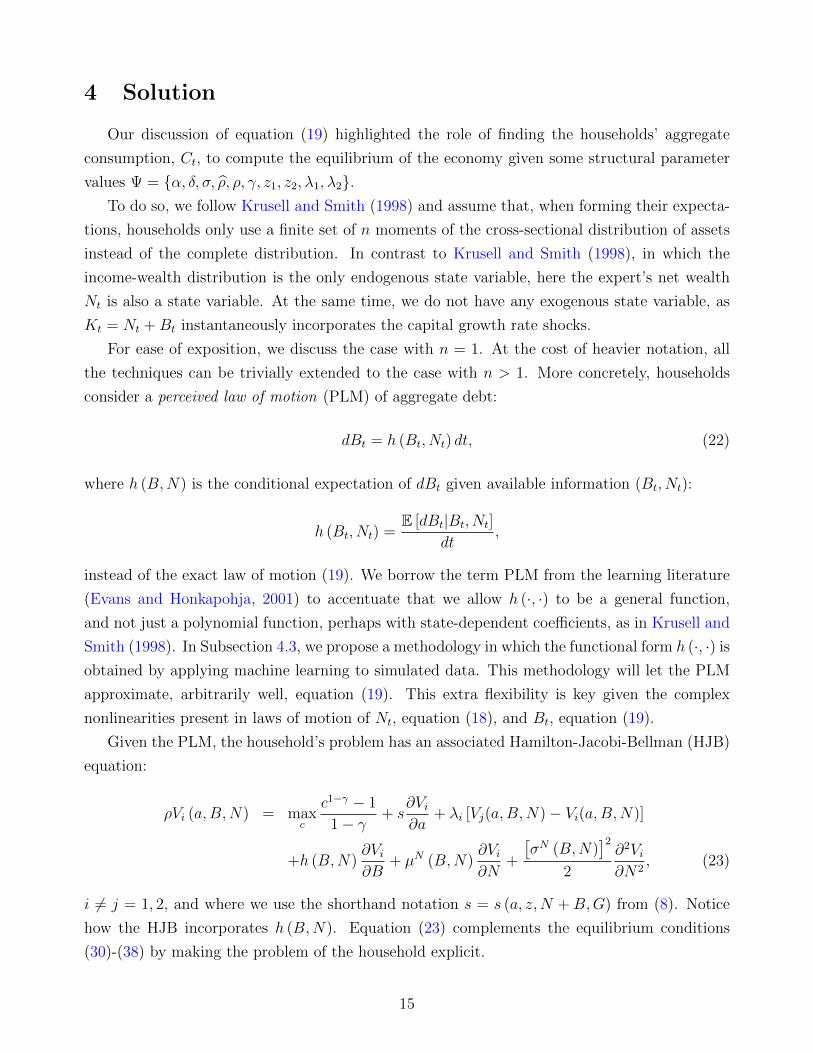
4 Solution

Our discussion of equation (19) highlighted the role of finding the households’ aggregate

consumption, Ct, to compute the equilibrium of the economy given some structural parameter

values Ψ = α, δ, σ, ρ, ρ, γ, z1, z2, λ1, λ2.To do so, we follow Krusell and Smith (1998) and assume that, when forming their expecta-

tions, households only use a finite set of n moments of the cross-sectional distribution of assets

instead of the complete distribution. In contrast to Krusell and Smith (1998), in which the

income-wealth distribution is the only endogenous state variable, here the expert’s net wealth

Nt is also a state variable. At the same time, we do not have any exogenous state variable, as

Kt = Nt +Bt instantaneously incorporates the capital growth rate shocks.

For ease of exposition, we discuss the case with n = 1. At the cost of heavier notation, all

the techniques can be trivially extended to the case with n > 1. More concretely, households

consider a perceived law of motion (PLM) of aggregate debt:

dBt = h (Bt, Nt) dt, (22)

where h (B,N) is the conditional expectation of dBt given available information (Bt, Nt):

h (Bt, Nt) =E [dBt|Bt, Nt]

dt,

instead of the exact law of motion (19). We borrow the term PLM from the learning literature

(Evans and Honkapohja, 2001) to accentuate that we allow h (·, ·) to be a general function,

and not just a polynomial function, perhaps with state-dependent coefficients, as in Krusell and

Smith (1998). In Subsection 4.3, we propose a methodology in which the functional form h (·, ·) is

obtained by applying machine learning to simulated data. This methodology will let the PLM

approximate, arbitrarily well, equation (19). This extra flexibility is key given the complex

nonlinearities present in laws of motion of Nt, equation (18), and Bt, equation (19).

Given the PLM, the household’s problem has an associated Hamilton-Jacobi-Bellman (HJB)

equation:

ρVi (a,B,N) = maxc

c1−γ − 1

1− γ+ s

∂Vi∂a

+ λi [Vj(a,B,N)− Vi(a,B,N)]

+h (B,N)∂Vi∂B

+ µN (B,N)∂Vi∂N

+

[σN (B,N)

]22

∂2Vi∂N2

, (23)

i 6= j = 1, 2, and where we use the shorthand notation s = s (a, z,N +B,G) from (8). Notice

how the HJB incorporates h (B,N). Equation (23) complements the equilibrium conditions

(30)-(38) by making the problem of the household explicit.

15

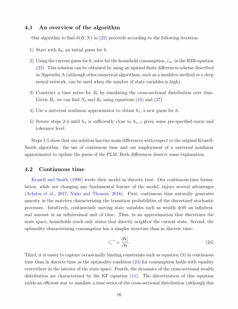
4.1 An overview of the algorithm

Our algorithm to find h(B,N) in (22) proceeds according to the following iteration:

1) Start with h0, an initial guess for h.

2) Using the current guess for h, solve for the household consumption, cm, in the HJB equation

(23). This solution can be obtained by using an upwind finite differences scheme described

in Appendix A (although other numerical algorithms, such as a meshfree method or a deep

neural network, can be used when the number of state variables is high).

3) Construct a time series for Bt by simulating the cross-sectional distribution over time.

Given Bt, we can find Nt and Kt using equations (18) and (37).

4) Use a universal nonlinear approximator to obtain h1, a new guess for h.

5) Iterate steps 2-4 until hn is sufficiently close to hn−1 given some pre-specified norm and

tolerance level.

Steps 1-5 show that our solution has two main differences with respect to the original Krusell-

Smith algorithm: the use of continuous time and our employment of a universal nonlinear

approximator to update the guess of the PLM. Both differences deserve some explanation.

4.2 Continuous time

Krusell and Smith (1998) wrote their model in discrete time. Our continuous-time formu-

lation, while not changing any fundamental feature of the model, enjoys several advantages

(Achdou et al., 2017; Nuno and Thomas, 2016). First, continuous time naturally generates

sparsity in the matrices characterizing the transition probabilities of the discretized stochastic

processes. Intuitively, continuously moving state variables such as wealth drift an infinitesi-

mal amount in an infinitesimal unit of time. Thus, in an approximation that discretizes the

state space, households reach only states that directly neighbor the current state. Second, the

optimality characterizing consumption has a simpler structure than in discrete time:

c−γi =∂Vi∂a

. (24)

Third, it is easier to capture occasionally binding constraints such as equation (9) in continuous

time than in discrete time as the optimality condition (24) for consumption holds with equality

everywhere in the interior of the state space. Fourth, the dynamics of the cross-sectional wealth

distribution are characterized by the KF equation (14). The discretization of this equation

yields an efficient way to simulate a time series of the cross-sectional distribution (although this

16

can also be performed in discrete time, as in Rıos-Rull 1997, Reiter 2009, and Young 2010, at

some cost).

We simulate T periods of the economy with a constant time step ∆t. We start from the

initial income-wealth distribution at the DSS (although we could pick other values). A number

of initial samples are discarded as a burn-in. If the time step is small enough, we have

Btj+∆t = Btj +

∫ tj+∆t

tj

dBs = Btj +

∫ tj+∆t

tj

h (Bs, Ns) ds ≈ Btj + h(Btj , Ntj

)∆t.

Our simulation(S, h

)is composed of a vector of inputs S = s1, s2, ..., sJ, where sj =

s1j , s

2j

=Btj , Ntj

are samples of aggregate debt and the expert’s net wealth at J random

times tj ∈ [0, T ], and a vector of outputs h =h1, h2..., hJ

, where

hj ≡Btj+∆t −Btj

∆t

are samples of the growth rate of Bt. The evaluation times tj should be random and uniformly

distributed over [0, T ] as, ideally, samples should be independent.

4.3 Neural networks: A universal nonlinear approximator

In the original Krusell-Smith algorithm, the law of motion linking the mean of capital tomor-

row and the mean of capital today is log-linear, with the coefficients in that function depending

on the aggregate shock. This approximation is highly accurate due to the near log-linearity

of their models in the vicinity of the DSS. Indeed, in such a model, the DSS and SSS almost

coincide. But, as shown in equations (18) and (19), this linearity of the law of motion of the

endogenous variables with respect to other endogenous variables does not extend to our model.

This nonlinear structure causes two problems. First, we face the approximation problem:

we need an algorithm that searches for an unknown nonlinear functional instead of a simple

linear regression with aggregate-state-dependent coefficients. Second, we need to tackle the

extrapolation problem. While the theoretical domain of Bt and Nt is unbounded, practical

computation requires limiting it to a compact subset of R2 large enough as to prevent boundary

conditions from altering the solution in the subregion where most of the ergodic distribution

accumulates. However, precisely because we deal with such a large area, the simulation in step

3 of the algorithm in Subsection 4.1 never visits an ample region of the state space. Thus, the

approximation algorithm should not only provide an accurate nonlinear approximation in the

visited region, but also a “reasonable” extrapolation to the rest of the state space. We will

return to what “reasonable” means in this context momentarily.

To address these two problems, we employ a nonlinear approximation technique based on

17

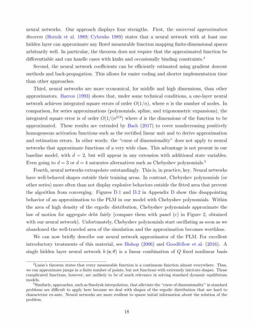
neural networks. Our approach displays four strengths. First, the universal approximation

theorem (Hornik et al. 1989; Cybenko 1989) states that a neural network with at least one

hidden layer can approximate any Borel measurable function mapping finite-dimensional spaces

arbitrarily well. In particular, the theorem does not require that the approximated function be

differentiable and can handle cases with kinks and occasionally binding constraints.4

Second, the neural network coefficients can be efficiently estimated using gradient descent

methods and back-propagation. This allows for easier coding and shorter implementation time

than other approaches.

Third, neural networks are more economical, for middle and high dimensions, than other

approximators. Barron (1993) shows that, under some technical conditions, a one-layer neural

network achieves integrated square errors of order O(1/n), where n is the number of nodes. In

comparison, for series approximations (polynomials, spline, and trigonometric expansions), the

integrated square error is of order O(1/(n2/d) where d is the dimensions of the function to be

approximated. These results are extended by Bach (2017) to cover nondecreasing positively

homogeneous activation functions such as the rectified linear unit and to derive approximation

and estimation errors. In other words: the “curse of dimensionality” does not apply to neural

networks that approximate functions of a very wide class. This advantage is not present in our

baseline model, with d = 2, but will appear in any extension with additional state variables.

Even going to d = 3 or d = 4 saturates alternatives such as Chebyshev polynomials.5

Fourth, neural networks extrapolate outstandingly. This is, in practice, key. Neural networks

have well-behaved shapes outside their training areas. In contrast, Chebyshev polynomials (or

other series) more often than not display explosive behaviors outside the fitted area that prevent

the algorithm from converging. Figures D.1 and D.2 in Appendix D show this disappointing

behavior of an approximation to the PLM in our model with Chebyshev polynomials. Within

the area of high density of the ergodic distribution, Chebyshev polynomials approximate the

law of motion for aggregate debt fairly (compare them with panel (c) in Figure 2, obtained

with our neural network). Unfortunately, Chebyshev polynomials start oscillating as soon as we

abandoned the well-traveled area of the simulation and the approximation becomes worthless.

We can now briefly describe our neural network approximator of the PLM. For excellent

introductory treatments of this material, see Bishop (2006) and Goodfellow et al. (2016). A

single hidden layer neural network h (s; θ) is a linear combination of Q fixed nonlinear basis

4Lusin’s theorem states that every measurable function is a continuous function almost everywhere. Thus,we can approximate jumps in a finite number of points, but not functions with extremely intricate shapes. Thosecomplicated functions, however, are unlikely to be of much relevance in solving standard dynamic equilibriummodels.

5Similarly, approaches, such as Smolyak interpolation, that alleviate the “curse of dimensionality” in standardproblems are difficult to apply here because we deal with shapes of the ergodic distribution that are hard tocharacterize ex-ante. Neural networks are more resilient to sparse initial information about the solution of theproblem.

18

(i.e., activation) functions φ(·):

h (s; θ) = θ20 +

Q∑q=1

θ2qφ

(θ1

0,q +2∑i=1

θ1i,qs

i

), (25)

where s is a two-dimensional input and θ a vector of coefficients (i.e., weights):

θ =(θ2

0, θ21, ..., θ

2Q, θ

10,1, θ

11,1, θ

12,1, ..., θ

10,Q, θ

11,Q, θ

12,Q

).

We call θ “coefficients,” as they represent a numerical entity, in comparison with the struc-

tural parameters, Ψ, that have a sharp economic interpretation. Thus, the neural network

provides a flexible parametric function h that determines the growth rate of aggregate debt

hj = h (sj; θ) , j = 1, .., J.

We pick, as an activation function, a softplus function, φ(x) = log(1 + ex) for a given input

x. The softplus function has a simple sigmoid derivative, which avoids some of the problems

caused by the presence of a kink in rectified linear units, a popular choice in other fields, while

keeping an efficient computation and gradient propagation.

The size of the hidden layer is determined by Q. This hypercoefficient can be set by reg-

ularization or, in simple problems, by trial-and-error. In our case, we set Q = 16 because the

cost of a larger hidden layer is small. The neural network (25) can be generalized to include

additional hidden layers. In that case, the network is called a deep neural network. However,

for the problem of approximating a two-dimensional function, a single layer is enough.

The vector of coefficients θ is selected to minimize the quadratic error function E(θ; S, h

)given a simulation

(S, h

):

θ∗ = arg maxθE(θ; S, h

)= arg max

θ

1

2

J∑j=1

∥∥∥h (sj; θ)− hj∥∥∥2

.

A standard approach to performing this minimization in neural networks is the batch gradient

descent algorithm. Appendix B describes the training of the network and how we handle possible

local minima.

Finally, notice that the algorithm is massively parallel, either in CPUs, GPUs, or FPGAs

(and, in the middle run, in the new generation of dedicated AI accelerators such as TPUs

specially designed for this class of problems). This is a most convenient feature for scaling and

estimation that other alternative solution approaches do not enjoy.

19

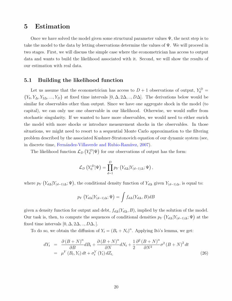
5 Estimation

Once we have solved the model given some structural parameter values Ψ, the next step is to

take the model to the data by letting observations determine the values of Ψ. We will proceed in

two stages. First, we will discuss the simple case where the econometrician has access to output

data and wants to build the likelihood associated with it. Second, we will show the results of

our estimation with real data.

5.1 Building the likelihood function

Let us assume that the econometrician has access to D + 1 observations of output, Y D0 =

Y0, Y∆, Y2∆, ..., YD at fixed time intervals [0,∆, 2∆, .., D∆]. The derivations below would be

similar for observables other than output. Since we have one aggregate shock in the model (to

capital), we can only use one observable in our likelihood. Otherwise, we would suffer from

stochastic singularity. If we wanted to have more observables, we would need to either enrich

the model with more shocks or introduce measurement shocks in the observables. In those

situations, we might need to resort to a sequential Monte Carlo approximation to the filtering

problem described by the associated Kushner-Stratonovich equation of our dynamic system (see,

in discrete time, Fernandez-Villaverde and Rubio-Ramırez, 2007).

The likelihood function LD(Y D

0 |Ψ)

for our observations of output has the form:

LD(Y D

0 |Ψ)

=D∏d=1

pY(Yd∆|Y(d−1)∆; Ψ

),

where pY(Yd∆|Y(d−1)∆; Ψ

), the conditional density function of Yd∆ given Y(d−1)∆, is equal to:

pY(Yd∆|Y(d−1)∆; Ψ

)=

∫fd∆(Yd∆, B)dB

given a density function for output and debt, fd∆(Yd∆, B), implied by the solution of the model.

Our task is, then, to compute the sequences of conditional densities pY(Yd∆|Y(d−1)∆; Ψ

)at the

fixed time intervals [0,∆, 2∆, .., D∆, ].

To do so, we obtain the diffusion of Yt = (Bt +Nt)α. Applying Ito’s lemma, we get:

dYt =∂ (B +N)α

∂BdBt +

∂ (B +N)α

∂NdNt +

1

2

∂2 (B +N)α

∂N2σ2 (B +N)2 dt

= µY (Bt, Yt) dt+ σYt (Yt) dZt, (26)

20

where:

µY (Bt, Yt) = αYα−1α

t

h(Bt, Y

1αt −Bt) + αYt +

[(α− 1)σ2

2− δ]Y

1αt

−

(αY

α−1α

t − δ − σ2 Y1αt

Y1αt −Bt

)Bt − ρ

(Y

1αt −Bt

),

and σY (Yt) = ασYt.

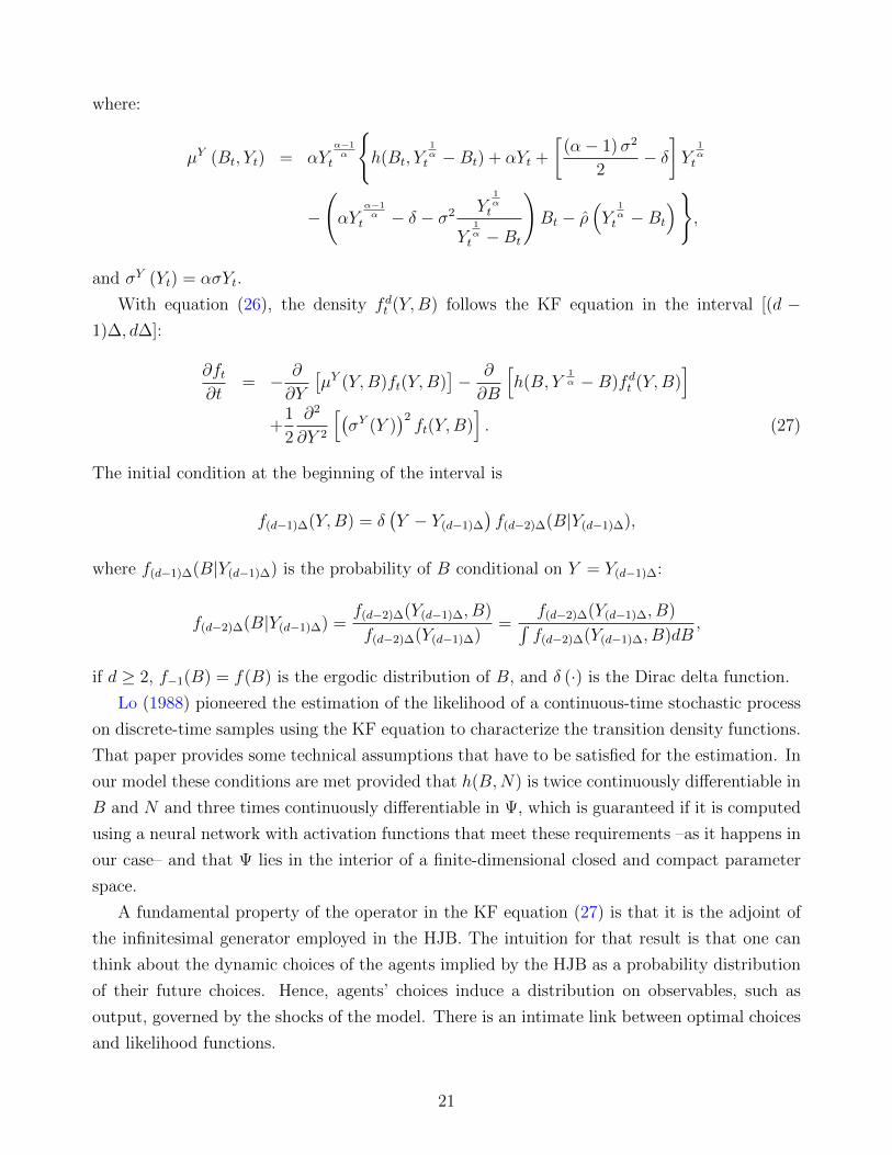
With equation (26), the density fdt (Y,B) follows the KF equation in the interval [(d −1)∆, d∆]:

∂ft∂t

= − ∂

∂Y

[µY (Y,B)ft(Y,B)

]− ∂

∂B

[h(B, Y

1α −B)fdt (Y,B)

]+

1

2

∂2

∂Y 2

[(σY (Y )

)2ft(Y,B)

]. (27)

The initial condition at the beginning of the interval is

f(d−1)∆(Y,B) = δ(Y − Y(d−1)∆

)f(d−2)∆(B|Y(d−1)∆),

where f(d−1)∆(B|Y(d−1)∆) is the probability of B conditional on Y = Y(d−1)∆:

f(d−2)∆(B|Y(d−1)∆) =f(d−2)∆(Y(d−1)∆, B)

f(d−2)∆(Y(d−1)∆)=

f(d−2)∆(Y(d−1)∆, B)∫f(d−2)∆(Y(d−1)∆, B)dB

,

if d ≥ 2, f−1(B) = f(B) is the ergodic distribution of B, and δ (·) is the Dirac delta function.

Lo (1988) pioneered the estimation of the likelihood of a continuous-time stochastic process

on discrete-time samples using the KF equation to characterize the transition density functions.

That paper provides some technical assumptions that have to be satisfied for the estimation. In

our model these conditions are met provided that h(B,N) is twice continuously differentiable in

B and N and three times continuously differentiable in Ψ, which is guaranteed if it is computed

using a neural network with activation functions that meet these requirements –as it happens in

our case– and that Ψ lies in the interior of a finite-dimensional closed and compact parameter

space.

A fundamental property of the operator in the KF equation (27) is that it is the adjoint of

the infinitesimal generator employed in the HJB. The intuition for that result is that one can

think about the dynamic choices of the agents implied by the HJB as a probability distribution

of their future choices. Hence, agents’ choices induce a distribution on observables, such as

output, governed by the shocks of the model. There is an intimate link between optimal choices

and likelihood functions.

21

This result is remarkable since it means that the solution of the KF equation amounts to

transposing and inverting a sparse matrix that has already been computed when we solved the

HJB. This provides a highly efficient way of evaluating the likelihood after the model is solved.6

In Appendix C, we briefly describe how to build the likelihood function of the model when

we also add microeconomic observations from the cross-sectional distribution of assets.

5.2 Maximizing the likelihood

Once we have evaluated the likelihood, we can either maximize it or perform Bayesian

inference relying on a posterior sampler. In this paper, for simplicity, we follow the former

approach. Also, since we are dealing with a novel approach to solution and estimation of

models with heterogeneous agents, we keep the estimation as transparent as possible by fixing

most of the structural parameters at conventional calibrated values for the U.S. economy. Also,

we use only aggregate variables.

We will rely on U.S. quarterly output observations for 1984.Q1-2017.Q4, with bandpass filter

keeping frequencies between 20 and 60 quarters (between 5 and 15 years). We start in 1984, as

often done in the literature, to focus on capturing the dynamics that have governed aggregate

fluctuations in the U.S. after the arrival of the Great Moderation (Galı and Gambetti, 2009).

See also the updated evidence in Liu et al. (2018), who document how the Great Moderation

has survived the 2007 financial crisis. We bandpass the data to eliminate long-run trends and to

skip the business cycle frequencies caused by productivity shocks and monetary policy shocks

our model is not designed to account for. However, our methodology does not depend on this

filtering and a richer model could be estimated with raw data without theoretical problems.

Parameter Value Description Source/Targetα 0.35 capital share standard

δ 0.1 capital depreciation standard

γ 2 risk aversion standard

ρ 0.05 households’ discount rate standard

λ1 0.986 transition rate unemp.-to-employment monthly job finding rate of 0.3

λ2 0.052 transition rate employment-to-unemp. unemployment rate 5%

z1 0.72 income in unemployment state Hall and Milgrom (2008)

z2 1.015 income in employment state E (y) = 1ρ 0.0497 experts’ discount rate K/N = 2

Table 1: Baseline parameterization.

6If the KF would become numerically cumbersome in more general models, we could construct Hermitepolynomial expansions of the (exact but unknown) likelihood as in Aıt-Sahalia (2002). We could also considermethods of moments in continuous time such as those pioneered by Andersen and Lund (1997) and Chacko andViceira (2003).

22

In terms of the fixed parameters, the capital share, α, is taken to be 0.35 and the depreciation

rate of capital, δ, is 0.1 (all rates are annual). The discount rate, ρ, is set to 0.05. The risk

aversion of the households γ is set to 2. These are standard values in the business cycle literature

to match the investment-output ratio and the rate of return on capital.

The idiosyncratic income process parameters are calibrated following our interpretation of

state 1 as unemployment and state 2 as employment. The transition rates between unemploy-

ment and employment (λ1, λ2) are chosen such that (i) the unemployment rate λ2/ (λ1 + λ2)

is 5% and (ii) the job finding rate is 0.3 at a monthly frequency or λ1 = 0.986 at an annual

frequency. These numbers describe the ‘U.S’ labor market calibration in Blanchard and Galı

(2010).7 We normalize average income z = λ2

λ1+λ2z1 + λ1

λ1+λ2z2 to 1. We also set z1 equal to 71%

of z2, as in Hall and Milgrom (2008). Both targets allow us to solve for z1 and z2. We set the

experts’ discount rate ρ to ensure that the leverage ratio K/N in the DSS is nearly 2, which is

roughly the average leverage from a Compustat sample of nonfinancial corporations. Table 1

summarizes our baseline calibration.

We solve the model according to the algorithm in Section 4. We use four Monte Carlo

simulations of 5,500 years, each at a monthly frequency. We initialize the model at the DSS,

and we disregard the first 500 years as a burn-in. We compute the PLM based on simulations

on a region of the state space.8

Then, we evaluate the likelihood of the observations on U.S. output for different values of

σ, the volatility of the aggregate shock and, therefore, the most interesting parameters in terms

of the properties of the model. While doing so, we keep all the other parameter values fixed at

their calibrated quantities. We maximize the likelihood function by searching on a grid between

0.013 and 0.015 with a step 0.0002 (we played extensively with σ values to determine the region

of high likelihood before starting the grid search).

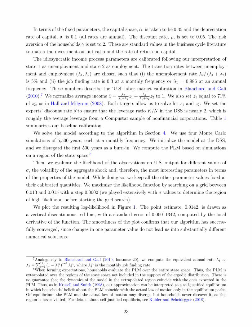
We plot the resulting log-likelihood in Figure 1. The point estimate, 0.0142, is drawn as

a vertical discontinuous red line, with a standard error of 0.00011342, computed by the local

derivative of the function. The smoothness of the plot confirms that our algorithm has success-

fully converged, since changes in one parameter value do not lead us into substantially different

numerical solutions.

7Analogously to Blanchard and Galı (2010, footnote 20), we compute the equivalent annual rate λ1 as

λ1 =∑12

i=1 (1− λm1 )i−1

λm1 , where λm1 is the monthly job finding rate.8When forming expectations, households evaluate the PLM over the entire state space. Thus, the PLM is

extrapolated over the regions of the state space not included in the support of the ergodic distribution. There isno guarantee that the dynamics of the model in the extrapolated region coincide with the ones expected in thePLM. Thus, as in Krusell and Smith (1998), our approximation can be interpreted as a self-justified equilibriumin which households’ beliefs about the PLM coincide with the actual law of motion only in the equilibrium paths.Off-equilibrium, the PLM and the actual law of motion may diverge, but households never discover it, as thisregion is never visited. For details about self-justified equilibria, see Kubler and Scheidegger (2018).

23

0.013 0.0132 0.0134 0.0136 0.0138 0.014 0.0142 0.0144 0.0146 0.0148 0.015-338.3

-338.25

-338.2

-338.15

-338.1

-338.05

-338

-337.95

-337.9

-337.85

-337.8

Figure 1: Log-likelihood for different values of σ and point estimate.

6 Quantitative results

This section presents the results generated by our solution algorithm with the parameter

values from Section 5. We will report, first, the PLM for aggregate debt, h(B,N) and assess

its accuracy as a solution. Next, we will explore the phase diagram of the model and explain,

through the dynamic responses of the model to an aggregate shock, why we find several SSS(s).

After having discussed the convergence properties of the SSS(s), and the random fluctuations

around those, and documented the presence of time-varying aggregate risk in our economy, we

will analyze the role of the value of σ in determining the multiplicity of SSS(s). We will close

by looking at the aggregate ergodic distribution of debt and equity.

6.1 The PLM

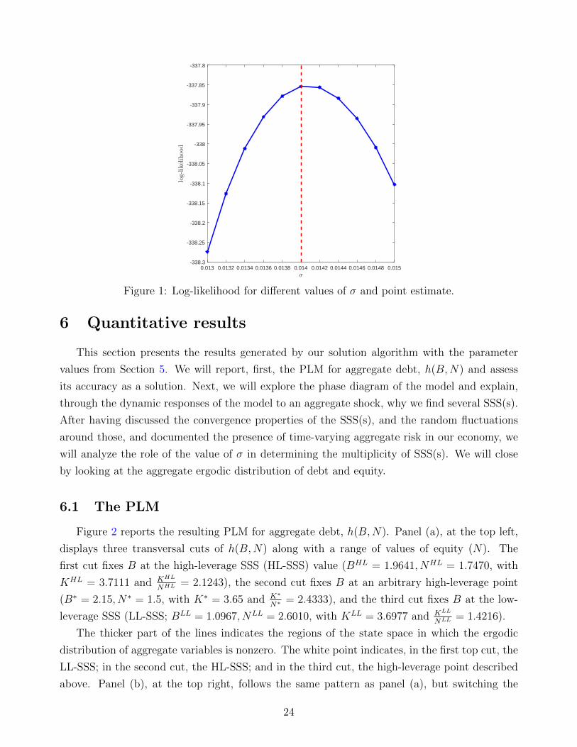
Figure 2 reports the resulting PLM for aggregate debt, h(B,N). Panel (a), at the top left,

displays three transversal cuts of h(B,N) along with a range of values of equity (N). The

first cut fixes B at the high-leverage SSS (HL-SSS) value (BHL = 1.9641, NHL = 1.7470, with

KHL = 3.7111 and KHL

NHL = 2.1243), the second cut fixes B at an arbitrary high-leverage point

(B∗ = 2.15, N∗ = 1.5, with K∗ = 3.65 and K∗

N∗ = 2.4333), and the third cut fixes B at the low-

leverage SSS (LL-SSS; BLL = 1.0967, NLL = 2.6010, with KLL = 3.6977 and KLL

NLL = 1.4216).

The thicker part of the lines indicates the regions of the state space in which the ergodic

distribution of aggregate variables is nonzero. The white point indicates, in the first top cut, the

LL-SSS; in the second cut, the HL-SSS; and in the third cut, the high-leverage point described

above. Panel (b), at the top right, follows the same pattern as panel (a), but switching the

24

1 1.5 2 2.5 3 3.5-0.06

-0.04

-0.02

0

0.02

0.04

0.06

0.08

0.5 1 1.5 2 2.5 3-0.15

-0.1

-0.05

0

0.05

0.1

-0.15

-0.1

-0.05

0

1

0.05

0.1

1.53

2 2.52

2.5 1.5

Figure 2: The PLM h(B,N) and transversal cuts.Note: White points in panels (a) and (b) indicate the LL-SSS, the HL-SSS, and an arbitrary high-leverage point.

The thicker part of the lanes in panels (a) and (b) and the shaded area in panel (c) displays the region of the

PLM visited in the ergodic distribution. The thin red line is the “zero” level intersected by the PLM.

roles of equity (N) and debt (B). Finally, panel (c), at the bottom, shows the complete three-

dimensional representation of the PLM. The shaded area in this panel highlights the region of

the PLM visited in the ergodic distribution with nontrivial positive probability. The thin red

line is the “zero” level intersected by the PLM: to the right of the line, aggregate debt falls, and

to the left, it grows.

Figure 2 demonstrates the nonlinearity of h(B,N) even within the area of the ergodic dis-

tribution that has positive mass. The agents in our economy expect different growth rates of

Bt in each region of the state space, with the function switching from concave to convex along

the way. While this argument is clear from the shape of panel (c), it encodes rich dynamics.

For instance, panel (b) shows how, as leverages increases, h(B,N) becomes steepper and, in

25

1 1.5 2 2.5 3 3.5-0.15

-0.1

-0.05

0

0.05

0.1

0.5 1 1.5 2 2.5 3-0.1

-0.05

0

0.05

0.1

-0.15

-0.1

-0.05

0

1

0.05

0.1

1.53

2 2.52

2.5 1.5

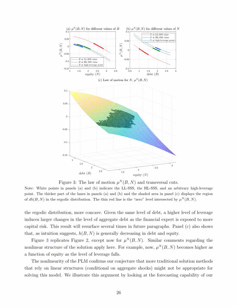
Figure 3: The law of motion µN(B,N) and transversal cuts.Note: White points in panels (a) and (b) indicate the LL-SSS, the HL-SSS, and an arbitrary high-leverage

point. The thicker part of the lanes in panels (a) and (b) and the shaded area in panel (c) displays the region

of dh(B,N) in the ergodic distribution. The thin red line is the “zero” level intersected by µN (B,N).

the ergodic distribution, more concave. Given the same level of debt, a higher level of leverage

induces larger changes in the level of aggregate debt as the financial expert is exposed to more

capital risk. This result will resurface several times in future paragraphs. Panel (c) also shows

that, as intuition suggests, h(B,N) is generally decreasing in debt and equity.

Figure 3 replicates Figure 2, except now for µN(B,N). Similar comments regarding the

nonlinear structure of the solution apply here. For example, now, µN(B,N) becomes higher as

a function of equity as the level of leverage falls.

The nonlinearity of the PLM confirms our conjecture that more traditional solution methods

that rely on linear structures (conditional on aggregate shocks) might not be appropriate for

solving this model. We illustrate this argument by looking at the forecasting capability of our

26

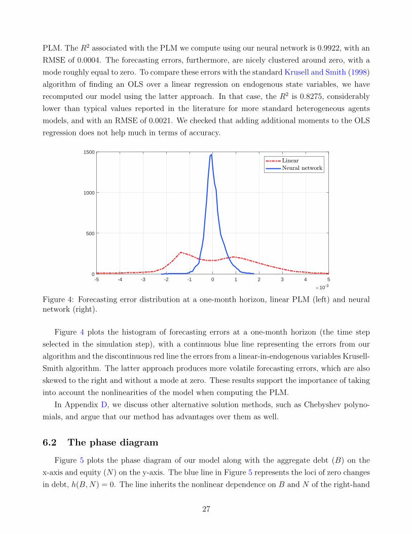
PLM. The R2 associated with the PLM we compute using our neural network is 0.9922, with an

RMSE of 0.0004. The forecasting errors, furthermore, are nicely clustered around zero, with a

mode roughly equal to zero. To compare these errors with the standard Krusell and Smith (1998)

algorithm of finding an OLS over a linear regression on endogenous state variables, we have

recomputed our model using the latter approach. In that case, the R2 is 0.8275, considerably

lower than typical values reported in the literature for more standard heterogeneous agents

models, and with an RMSE of 0.0021. We checked that adding additional moments to the OLS

regression does not help much in terms of accuracy.

-5 -4 -3 -2 -1 0 1 2 3 4 5

10-3

0

500

1000

1500

Figure 4: Forecasting error distribution at a one-month horizon, linear PLM (left) and neuralnetwork (right).

Figure 4 plots the histogram of forecasting errors at a one-month horizon (the time step

selected in the simulation step), with a continuous blue line representing the errors from our

algorithm and the discontinuous red line the errors from a linear-in-endogenous variables Krusell-

Smith algorithm. The latter approach produces more volatile forecasting errors, which are also

skewed to the right and without a mode at zero. These results support the importance of taking

into account the nonlinearities of the model when computing the PLM.

In Appendix D, we discuss other alternative solution methods, such as Chebyshev polyno-

mials, and argue that our method has advantages over them as well.

6.2 The phase diagram

Figure 5 plots the phase diagram of our model along with the aggregate debt (B) on the

x-axis and equity (N) on the y-axis. The blue line in Figure 5 represents the loci of zero changes

in debt, h(B,N) = 0. The line inherits the nonlinear dependence on B and N of the right-hand

27

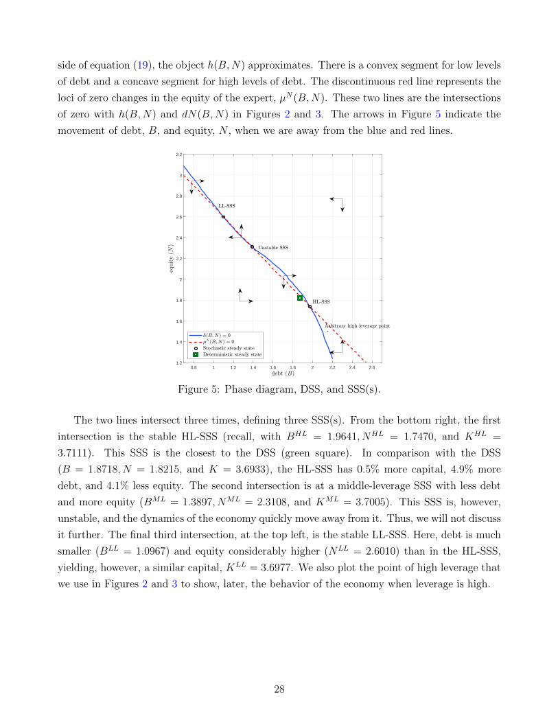
side of equation (19), the object h(B,N) approximates. There is a convex segment for low levels

of debt and a concave segment for high levels of debt. The discontinuous red line represents the

loci of zero changes in the equity of the expert, µN(B,N). These two lines are the intersections

of zero with h(B,N) and dN(B,N) in Figures 2 and 3. The arrows in Figure 5 indicate the

movement of debt, B, and equity, N , when we are away from the blue and red lines.

0.8 1 1.2 1.4 1.6 1.8 2 2.2 2.4 2.61.2

1.4

1.6

1.8

2

2.2

2.4

2.6

2.8

3

3.2

Figure 5: Phase diagram, DSS, and SSS(s).

The two lines intersect three times, defining three SSS(s). From the bottom right, the first

intersection is the stable HL-SSS (recall, with BHL = 1.9641, NHL = 1.7470, and KHL =

3.7111). This SSS is the closest to the DSS (green square). In comparison with the DSS

(B = 1.8718, N = 1.8215, and K = 3.6933), the HL-SSS has 0.5% more capital, 4.9% more

debt, and 4.1% less equity. The second intersection is at a middle-leverage SSS with less debt

and more equity (BML = 1.3897, NML = 2.3108, and KML = 3.7005). This SSS is, however,

unstable, and the dynamics of the economy quickly move away from it. Thus, we will not discuss

it further. The final third intersection, at the top left, is the stable LL-SSS. Here, debt is much

smaller (BLL = 1.0967) and equity considerably higher (NLL = 2.6010) than in the HL-SSS,

yielding, however, a similar capital, KLL = 3.6977. We also plot the point of high leverage that

we use in Figures 2 and 3 to show, later, the behavior of the economy when leverage is high.

28

6.3 Why do we have two stable SSS(s)?

To understand why we have two stable SSS(s) in Figure 5, first, recall the diffusion for the

expert’s net wealth in equation (34) and rewrite it in rates as:

dNt

Nt

=(αKα−1

t − δ − ρ)dt+ σ2Bt

Kt

N2t

dt+ σKt

Nt

dZt. (28)

The volatility term of (28), σKtNtdZt, reflects how the proportional effect on the expert’s

equity of a shock to capital is higher when her leverage level is high. Given that the expert

must absorb all the gains or losses from a shock to capital, the smaller the base of her equity in

relation to total capital, the larger the proportional drop in Nt.

The two drift terms of (28) explain why the rate of recovery of Nt from a negative shock to

capital is roughly independent of leverage. The first drift term,(αKα−1

t − δ − ρ)dt, does not

depend directly on Nt. The second drift term, σ2BtKtN2tdt, indicates that the rate of accumulation

of equity will be higher when Nt is small relative to Kt. However, since the term is multiplied

by σ2, a small quantity, the total effect on dNtNt

is muted.

Next, let us inspect the law of motion for debt, (19), and rearrange it as:

dBt =

((1− α)Kα

t − σ2Kt

Nt

Bt

)dt+ (αKα−1

t − δ)Btdt− Ctdt. (29)

The first drift term of (29),(

(1− α)Kαt − σ2Kt

NtBt

)dt, becomes smaller after a negative capital

shock: less capital lowers labor income, (1−α)Kαt , and σ2Kt

NtBt rises because the expert must be

compensated with a larger excess return for her higher leverage to be an equilibrium choice. High

leverage makes the reduction on this term larger. The second drift term of (29), (αKα−1t −δ)Btdt,

is bigger after a negative capital shock because the marginal productivity of capital goes up.

However, higher leverage means thatBt is low relative toKt and, hence, the whole term is smaller

than it would be with low leverage. Finally, households reduce their aggregate consumption, Ct,

to compensate for lower wages and higher risk-free interest rates, which increases dBt. However,

Ct only depends weakly on leverage. High leverage, through higher risk-free real interest rates

after a negative capital shock, induces more intertemporal substitution in consumption, but this

difference is quantitatively minor.

In summary: equations (28) and (29) show that, when leverage is high, i) the financial

expert’s equity falls more; ii) the recovery of this equity is roughly at the same rate as when

leverage is low; iii) debt increases less; and iv) consequently, capital recovery is slow.

We can gauge the quantitative size of these four points in Figure 6, where we display the

generalized impulse response functions (GIRFs) to a two-standard-deviations negative capital

shock. The GIRF is defined as the difference between the transition path if an initial shock hits

29

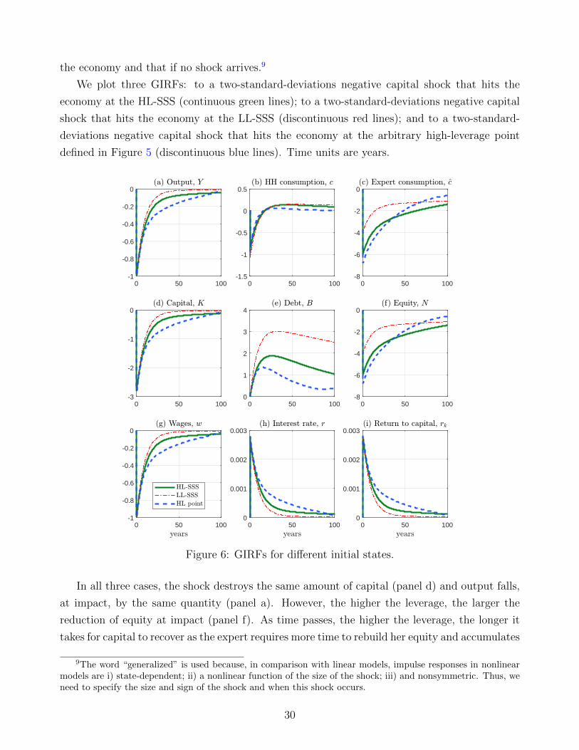
the economy and that if no shock arrives.9

We plot three GIRFs: to a two-standard-deviations negative capital shock that hits the

economy at the HL-SSS (continuous green lines); to a two-standard-deviations negative capital

shock that hits the economy at the LL-SSS (discontinuous red lines); and to a two-standard-

deviations negative capital shock that hits the economy at the arbitrary high-leverage point

defined in Figure 5 (discontinuous blue lines). Time units are years.

0 50 100-1

-0.8

-0.6

-0.4

-0.2

0

0 50 100-1.5

-1

-0.5

0

0.5

0 50 100-8

-6

-4

-2

0

0 50 100-3

-2

-1

0

0 50 1000

1

2

3

4

0 50 100-8

-6

-4

-2

0

0 50 100-1

-0.8

-0.6

-0.4

-0.2

0

0 50 1000

0.001

0.002

0.003

0 50 1000

0.001

0.002

0.003

Figure 6: GIRFs for different initial states.

In all three cases, the shock destroys the same amount of capital (panel d) and output falls,

at impact, by the same quantity (panel a). However, the higher the leverage, the larger the

reduction of equity at impact (panel f). As time passes, the higher the leverage, the longer it

takes for capital to recover as the expert requires more time to rebuild her equity and accumulates

9The word “generalized” is used because, in comparison with linear models, impulse responses in nonlinearmodels are i) state-dependent; ii) a nonlinear function of the size of the shock; iii) and nonsymmetric. Thus, weneed to specify the size and sign of the shock and when this shock occurs.

30

less debt (panel e). The lower debt is an equilibrium choice for households because the more

persistent risk-free rate (panel h) induces a mild reduction in household consumption (panel b).

The state-dependence of the GIRFs demonstrates the nonlinearities of our model. Further-

more, the two-standard-deviations shock is not large enough to send the economy away from the

basins of attraction of each SSS. An even larger shock or a shock closer to the frontier between

the two basins, by inducing a switch of basin, will have even stronger nonlinear effects (we will

return to this point below).

A central property of the GIRFs is their persistence. When leverage is high, even after

40 years, the economy is still around half a percentage point below its pre-shock level. The

dynamics of equity and debt accumulation propagate aggregate shocks in ways that are not

present in models without financial frictions.

The latter point is salient for the next step of our argument explaining the existence of

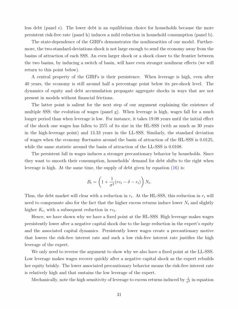
multiple SSS: the evolution of wages (panel g). When leverage is high, wages fall for a much

longer period than when leverage is low. For instance, it takes 19.08 years until the initial effect

of the shock one wages has fallen to 25% of its size in the HL-SSS (with as much as 30 years

in the high-leverage point) and 13.33 years in the LL-SSS. Similarly, the standard deviation

of wages when the economy fluctuates around the basin of attraction of the HL-SSS is 0.0125,

while the same statistic around the basin of attraction of the LL-SSS is 0.0108.

The persistent fall in wages induces a stronger precautionary behavior by households. Since

they want to smooth their consumption, households’ demand for debt shifts to the right when

leverage is high. At the same time, the supply of debt given by equation (16) is:

Bt =

(1 +

1

σ2(rct − δ − rt)

)Nt.

Thus, the debt market will clear with a reduction in rt. At the HL-SSS, this reduction in rt will

need to compensate also for the fact that the higher excess returns induce lower Nt and slightly

higher Kt, with a subsequent reduction in rct.

Hence, we have shown why we have a fixed point at the HL-SSS. High leverage makes wages

persistently lower after a negative capital shock due to the large reduction in the expert’s equity

and the associated capital dynamics. Persistently lower wages create a precautionary motive

that lowers the risk-free interest rate and such a low risk-free interest rate justifies the high

leverage of the expert.

We only need to reverse the argument to show why we also have a fixed point at the LL-SSS.

Low leverage makes wages recover quickly after a negative capital shock as the expert rebuilds

her equity briskly. The lower associated precautionary behavior means the risk-free interest rate

is relatively high and that sustains the low leverage of the expert.

Mechanically, note the high sensitivity of leverage to excess returns induced by 1σ2 in equation

31

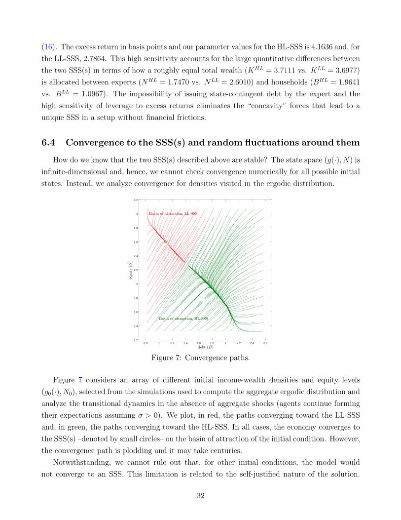
(16). The excess return in basis points and our parameter values for the HL-SSS is 4.1636 and, for

the LL-SSS, 2.7864. This high sensitivity accounts for the large quantitative differences between

the two SSS(s) in terms of how a roughly equal total wealth (KHL = 3.7111 vs. KLL = 3.6977)

is allocated between experts (NHL = 1.7470 vs. NLL = 2.6010) and households (BHL = 1.9641

vs. BLL = 1.0967). The impossibility of issuing state-contingent debt by the expert and the

high sensitivity of leverage to excess returns eliminates the “concavity” forces that lead to a

unique SSS in a setup without financial frictions.

6.4 Convergence to the SSS(s) and random fluctuations around them

How do we know that the two SSS(s) described above are stable? The state space (g(·), N) is

infinite-dimensional and, hence, we cannot check convergence numerically for all possible initial

states. Instead, we analyze convergence for densities visited in the ergodic distribution.

0.8 1 1.2 1.4 1.6 1.8 2 2.2 2.4 2.61.2

1.4

1.6

1.8

2

2.2

2.4

2.6

2.8

3

3.2

Figure 7: Convergence paths.

Figure 7 considers an array of different initial income-wealth densities and equity levels

(g0(·), N0), selected from the simulations used to compute the aggregate ergodic distribution and

analyze the transitional dynamics in the absence of aggregate shocks (agents continue forming

their expectations assuming σ > 0). We plot, in red, the paths converging toward the LL-SSS

and, in green, the paths converging toward the HL-SSS. In all cases, the economy converges to

the SSS(s) –denoted by small circles– on the basin of attraction of the initial condition. However,

the convergence path is plodding and it may take centuries.

Notwithstanding, we cannot rule out that, for other initial conditions, the model would

not converge to an SSS. This limitation is related to the self-justified nature of the solution.

32

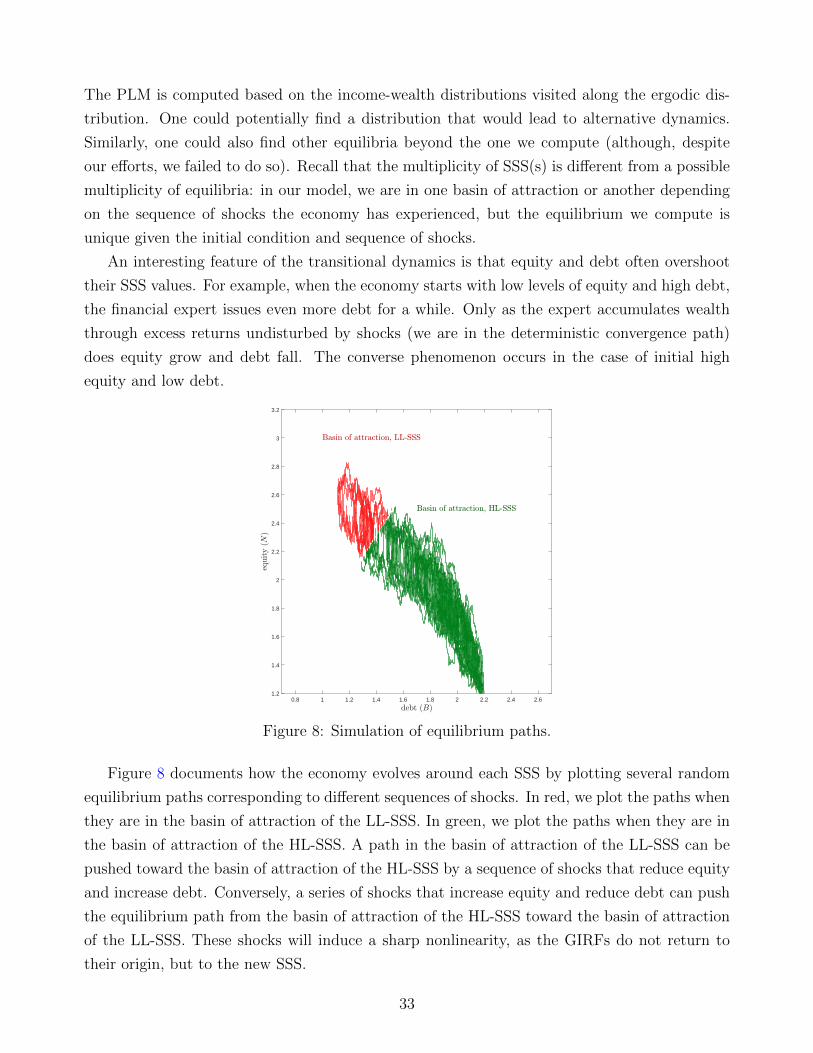
The PLM is computed based on the income-wealth distributions visited along the ergodic dis-

tribution. One could potentially find a distribution that would lead to alternative dynamics.

Similarly, one could also find other equilibria beyond the one we compute (although, despite

our efforts, we failed to do so). Recall that the multiplicity of SSS(s) is different from a possible

multiplicity of equilibria: in our model, we are in one basin of attraction or another depending

on the sequence of shocks the economy has experienced, but the equilibrium we compute is

unique given the initial condition and sequence of shocks.

An interesting feature of the transitional dynamics is that equity and debt often overshoot

their SSS values. For example, when the economy starts with low levels of equity and high debt,

the financial expert issues even more debt for a while. Only as the expert accumulates wealth

through excess returns undisturbed by shocks (we are in the deterministic convergence path)

does equity grow and debt fall. The converse phenomenon occurs in the case of initial high

equity and low debt.

0.8 1 1.2 1.4 1.6 1.8 2 2.2 2.4 2.61.2

1.4

1.6

1.8

2

2.2

2.4

2.6

2.8

3

3.2

Figure 8: Simulation of equilibrium paths.

Figure 8 documents how the economy evolves around each SSS by plotting several random

equilibrium paths corresponding to different sequences of shocks. In red, we plot the paths when

they are in the basin of attraction of the LL-SSS. In green, we plot the paths when they are in

the basin of attraction of the HL-SSS. A path in the basin of attraction of the LL-SSS can be

pushed toward the basin of attraction of the HL-SSS by a sequence of shocks that reduce equity

and increase debt. Conversely, a series of shocks that increase equity and reduce debt can push

the equilibrium path from the basin of attraction of the HL-SSS toward the basin of attraction

of the LL-SSS. These shocks will induce a sharp nonlinearity, as the GIRFs do not return to

their origin, but to the new SSS.

33

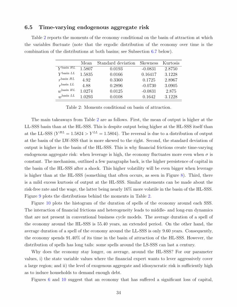
6.5 Time-varying endogenous aggregate risk

Table 2 reports the moments of the economy conditional on the basin of attraction at which

the variables fluctuate (note that the ergodic distribution of the economy over time is the

combination of the distributions at both basins; see Subsection 6.7 below).

Mean Standard deviation Skewness KurtosisY basin HL 1.5807 0.0193 -0.0831 2.8750Y basin LL 1.5835 0.0166 0.16417 3.1228rbasin HL 4.92 0.3360 0.1725 2.8967rbasin LL 4.88 0.2896 -0.0730 3.0905wbasin HL 1.0274 0.0125 -0.0831 2.875wbasin LL 1.0293 0.0108 0.1642 3.1228

Table 2: Moments conditional on basin of attraction.

The main takeaways from Table 2 are as follows. First, the mean of output is higher at the

LL-SSS basin than at the HL-SSS. This is despite output being higher at the HL-SSS itself than

at the LL-SSS (Y HL = 1.5824 > Y LL = 1.5804). The reversal is due to a distribution of output

at the basin of the LW-SSS that is more skewed to the right. Second, the standard deviation of

output is higher in the basin of the HL-SSS. This is why financial frictions create time-varying

endogenous aggregate risk: when leverage is high, the economy fluctuates more even when σ is

constant. The mechanism, outlined a few paragraphs back, is the higher persistence of capital in

the basin of the HL-SSS after a shock. This higher volatility will be even bigger when leverage

is higher than at the HL-SSS (something that often occurs, as seen in Figure 8). Third, there

is a mild excess kurtosis of output at the HL-SSS. Similar statements can be made about the

risk-free rate and the wage, the latter being nearly 16% more volatile in the basin of the HL-SSS.

Figure 9 plots the distributions behind the moments in Table 2.

Figure 10 plots the histogram of the duration of spells of the economy around each SSS.

The interaction of financial frictions and heterogeneity leads to middle- and long-run dynamics

that are not present in conventional business cycle models. The average duration of a spell of

the economy around the HL-SSS is 55.40 years, an extended period. On the other hand, the

average duration of a spell of the economy around the LL-SSS is only 9.60 years. Consequently,

the economy spends 91.40% of its time in the basin of attraction of the HL-SSS. However, the

distribution of spells has long tails: some spells around the LS-SSS can last a century.

Why does the economy stay longer, on average, around the HL-SSS? For our parameter

values, i) the state variable values where the financial expert wants to lever aggressively cover

a large region; and ii) the level of exogenous aggregate and idiosyncratic risk is sufficiently high

as to induce households to demand enough debt.

Figures 6 and 10 suggest that an economy that has suffered a significant loss of capital,

34

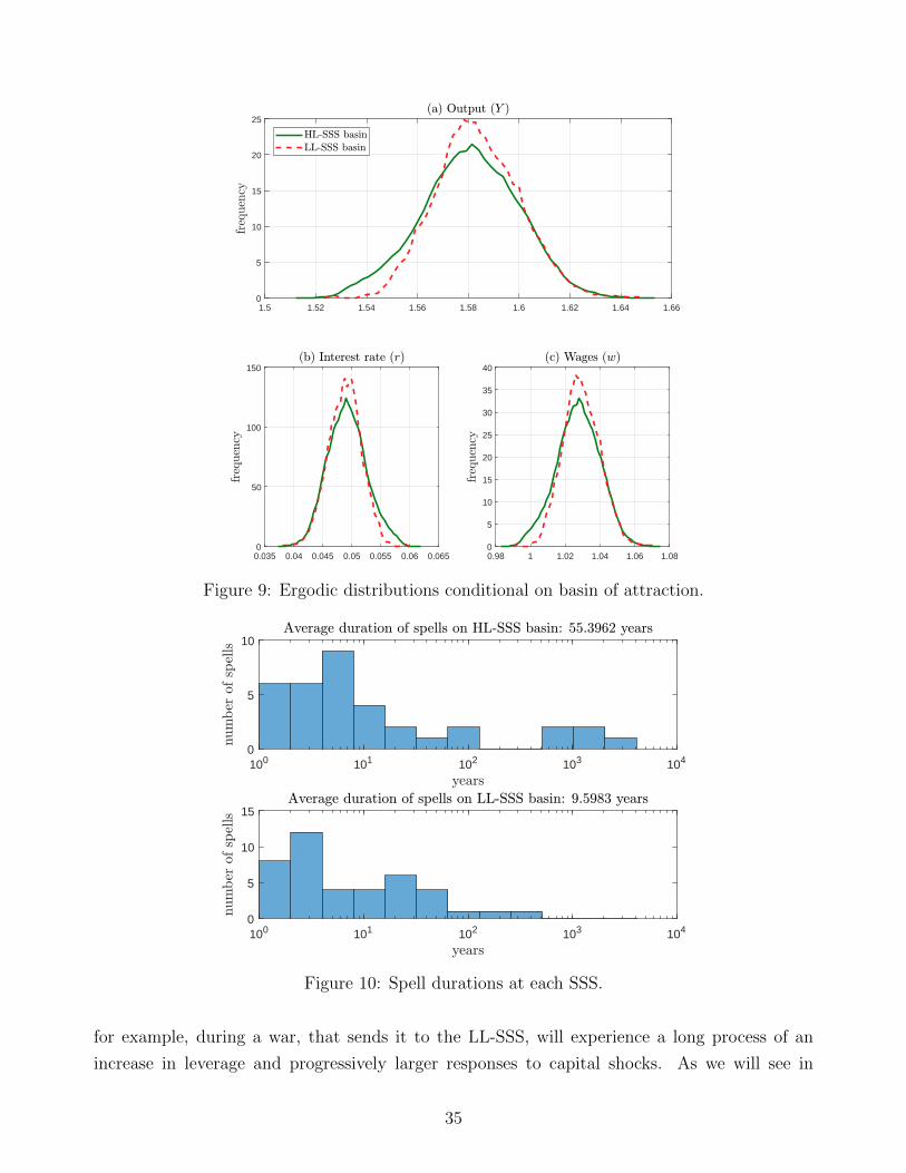
1.5 1.52 1.54 1.56 1.58 1.6 1.62 1.64 1.660

5

10

15

20

25

0.035 0.04 0.045 0.05 0.055 0.06 0.0650

50

100

150

0.98 1 1.02 1.04 1.06 1.080

5

10

15

20

25

30

35

40

Figure 9: Ergodic distributions conditional on basin of attraction.

100 101 102 103 1040

5

10

100 101 102 103 1040

5

10

15

Figure 10: Spell durations at each SSS.

for example, during a war, that sends it to the LL-SSS, will experience a long process of an

increase in leverage and progressively larger responses to capital shocks. As we will see in

35

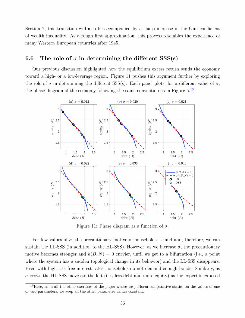
Section 7, this transition will also be accompanied by a sharp increase in the Gini coefficient

of wealth inequality. As a rough first approximation, this process resembles the experience of

many Western European countries after 1945.

6.6 The role of σ in determining the different SSS(s)

Our previous discussion highlighted how the equilibrium excess return sends the economy

toward a high- or a low-leverage region. Figure 11 pushes this argument further by exploring

the role of σ in determining the different SSS(s). Each panel plots, for a different value of σ,

the phase diagram of the economy following the same convention as in Figure 5.10

1 1.5 2 2.5

1.5

2

2.5

3

1 1.5 2 2.5

1.5

2

2.5

3

1 1.5 2 2.5

1.5

2

2.5

3

1 1.5 2 2.5

1.5

2

2.5

3

1 1.5 2 2.5

1.5

2

2.5

3

1 1.5 2 2.5

1.5

2

2.5

3

Figure 11: Phase diagram as a function of σ.

For low values of σ, the precautionary motive of households is mild and, therefore, we can

sustain the LL-SSS (in addition to the HL-SSS). However, as we increase σ, the precautionary

motive becomes stronger and h(B,N) = 0 curvier, until we get to a bifurcation (i.e., a point

where the system has a sudden topological change in its behavior) and the LL-SSS disappears.

Even with high risk-free interest rates, households do not demand enough bonds. Similarly, as

σ grows the HL-SSS moves to the left (i.e., less debt and more equity) as the expert is exposed

10Here, as in all the other exercises of the paper where we perform comparative statics on the values of oneor two parameters, we keep all the other parameter values constant.

36

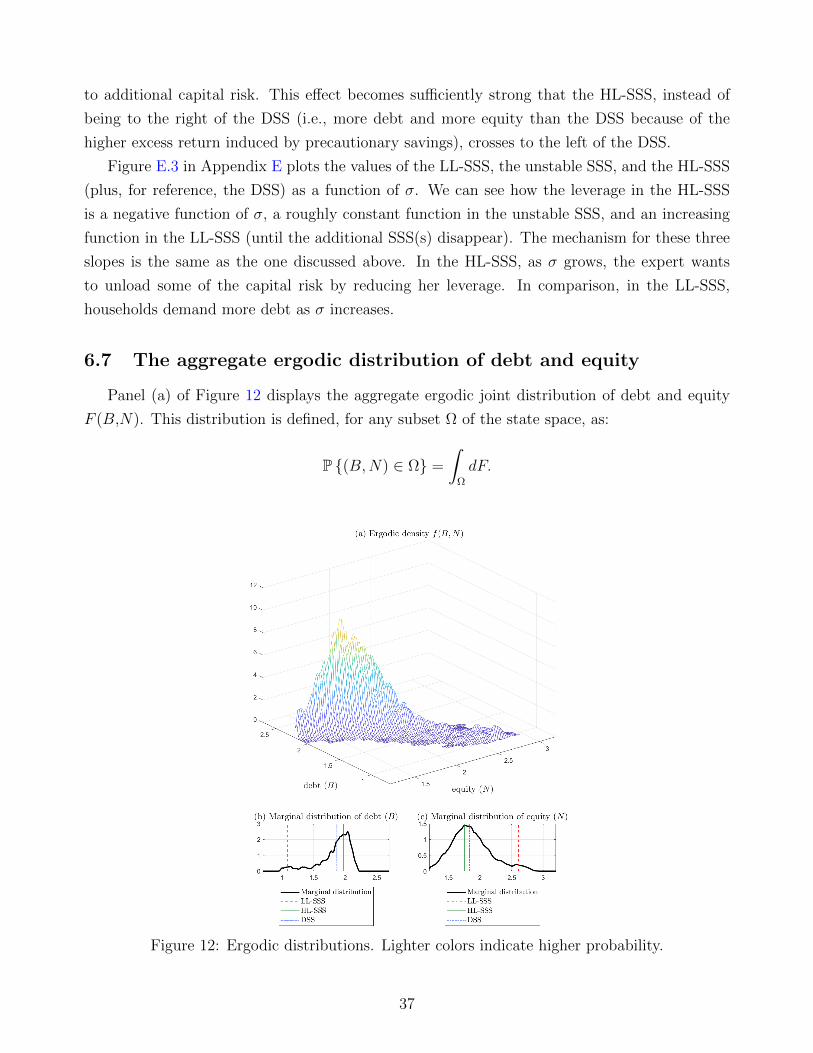
to additional capital risk. This effect becomes sufficiently strong that the HL-SSS, instead of

being to the right of the DSS (i.e., more debt and more equity than the DSS because of the

higher excess return induced by precautionary savings), crosses to the left of the DSS.

Figure E.3 in Appendix E plots the values of the LL-SSS, the unstable SSS, and the HL-SSS

(plus, for reference, the DSS) as a function of σ. We can see how the leverage in the HL-SSS

is a negative function of σ, a roughly constant function in the unstable SSS, and an increasing

function in the LL-SSS (until the additional SSS(s) disappear). The mechanism for these three

slopes is the same as the one discussed above. In the HL-SSS, as σ grows, the expert wants

to unload some of the capital risk by reducing her leverage. In comparison, in the LL-SSS,

households demand more debt as σ increases.

6.7 The aggregate ergodic distribution of debt and equity

Panel (a) of Figure 12 displays the aggregate ergodic joint distribution of debt and equity

F (B,N). This distribution is defined, for any subset Ω of the state space, as:

P (B,N) ∈ Ω =

∫Ω

dF.

Figure 12: Ergodic distributions. Lighter colors indicate higher probability.

37

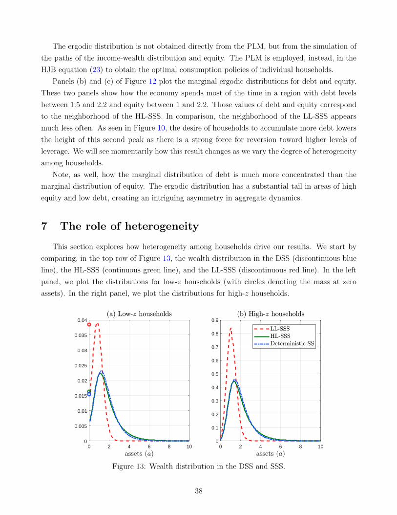
The ergodic distribution is not obtained directly from the PLM, but from the simulation of

the paths of the income-wealth distribution and equity. The PLM is employed, instead, in the

HJB equation (23) to obtain the optimal consumption policies of individual households.

Panels (b) and (c) of Figure 12 plot the marginal ergodic distributions for debt and equity.

These two panels show how the economy spends most of the time in a region with debt levels

between 1.5 and 2.2 and equity between 1 and 2.2. Those values of debt and equity correspond

to the neighborhood of the HL-SSS. In comparison, the neighborhood of the LL-SSS appears

much less often. As seen in Figure 10, the desire of households to accumulate more debt lowers

the height of this second peak as there is a strong force for reversion toward higher levels of

leverage. We will see momentarily how this result changes as we vary the degree of heterogeneity

among households.

Note, as well, how the marginal distribution of debt is much more concentrated than the

marginal distribution of equity. The ergodic distribution has a substantial tail in areas of high

equity and low debt, creating an intriguing asymmetry in aggregate dynamics.

7 The role of heterogeneity

This section explores how heterogeneity among households drive our results. We start by

comparing, in the top row of Figure 13, the wealth distribution in the DSS (discontinuous blue

line), the HL-SSS (continuous green line), and the LL-SSS (discontinuous red line). In the left

panel, we plot the distributions for low-z households (with circles denoting the mass at zero

assets). In the right panel, we plot the distributions for high-z households.

0 2 4 6 8 100

0.005

0.01

0.015

0.02

0.025

0.03

0.035

0.04

0 2 4 6 8 100

0.1

0.2

0.3

0.4

0.5

0.6

0.7

0.8

0.9

Figure 13: Wealth distribution in the DSS and SSS.

38

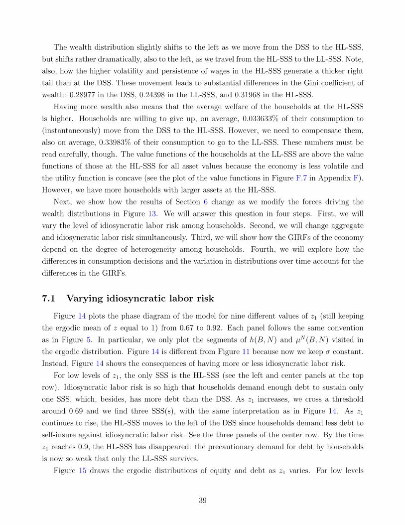
The wealth distribution slightly shifts to the left as we move from the DSS to the HL-SSS,

but shifts rather dramatically, also to the left, as we travel from the HL-SSS to the LL-SSS. Note,

also, how the higher volatility and persistence of wages in the HL-SSS generate a thicker right

tail than at the DSS. These movement leads to substantial differences in the Gini coefficient of

wealth: 0.28977 in the DSS, 0.24398 in the LL-SSS, and 0.31968 in the HL-SSS.

Having more wealth also means that the average welfare of the households at the HL-SSS

is higher. Households are willing to give up, on average, 0.033633% of their consumption to

(instantaneously) move from the DSS to the HL-SSS. However, we need to compensate them,

also on average, 0.33983% of their consumption to go to the LL-SSS. These numbers must be

read carefully, though. The value functions of the households at the LL-SSS are above the value

functions of those at the HL-SSS for all asset values because the economy is less volatile and

the utility function is concave (see the plot of the value functions in Figure F.7 in Appendix F).

However, we have more households with larger assets at the HL-SSS.

Next, we show how the results of Section 6 change as we modify the forces driving the

wealth distributions in Figure 13. We will answer this question in four steps. First, we will

vary the level of idiosyncratic labor risk among households. Second, we will change aggregate

and idiosyncratic labor risk simultaneously. Third, we will show how the GIRFs of the economy

depend on the degree of heterogeneity among households. Fourth, we will explore how the

differences in consumption decisions and the variation in distributions over time account for the

differences in the GIRFs.

7.1 Varying idiosyncratic labor risk

Figure 14 plots the phase diagram of the model for nine different values of z1 (still keeping

the ergodic mean of z equal to 1) from 0.67 to 0.92. Each panel follows the same convention

as in Figure 5. In particular, we only plot the segments of h(B,N) and µN(B,N) visited in

the ergodic distribution. Figure 14 is different from Figure 11 because now we keep σ constant.

Instead, Figure 14 shows the consequences of having more or less idiosyncratic labor risk.

For low levels of z1, the only SSS is the HL-SSS (see the left and center panels at the top

row). Idiosyncratic labor risk is so high that households demand enough debt to sustain only

one SSS, which, besides, has more debt than the DSS. As z1 increases, we cross a threshold

around 0.69 and we find three SSS(s), with the same interpretation as in Figure 14. As z1

continues to rise, the HL-SSS moves to the left of the DSS since households demand less debt to

self-insure against idiosyncratic labor risk. See the three panels of the center row. By the time

z1 reaches 0.9, the HL-SSS has disappeared: the precautionary demand for debt by households

is now so weak that only the LL-SSS survives.

Figure 15 draws the ergodic distributions of equity and debt as z1 varies. For low levels

39

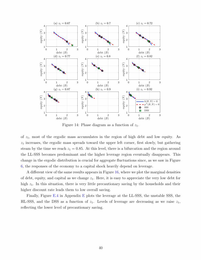
0 1 2 31

2

3

4

0 1 2 31

2

3

4

0 1 2 31

2

3

4

0 1 2 31

2

3

4

0 1 2 31

2

3

4

0 1 2 31

2

3

4

0 1 2 31

2

3

4

0 1 2 31

2

3

4

0 1 2 31

2

3

4

Figure 14: Phase diagram as a function of z1.

of z1, most of the ergodic mass accumulates in the region of high debt and low equity. As

z1 increases, the ergodic mass spreads toward the upper left corner, first slowly, but gathering

steam by the time we reach z1 = 0.85. At this level, there is a bifurcation and the region around

the LL-SSS becomes predominant and the higher leverage region eventually disappears. This

change in the ergodic distribution is crucial for aggregate fluctuations since, as we saw in Figure

6, the responses of the economy to a capital shock heavily depend on leverage.

A different view of the same results appears in Figure 16, where we plot the marginal densities

of debt, equity, and capital as we change z1. Here, it is easy to appreciate the very low debt for

high z1. In this situation, there is very little precautionary saving by the households and their

higher discount rate leads them to low overall saving.

Finally, Figure E.4 in Appendix E plots the leverage at the LL-SSS, the unstable SSS, the

HL-SSS, and the DSS as a function of z1. Levels of leverage are decreasing as we raise z1,

reflecting the lower level of precautionary saving.

40

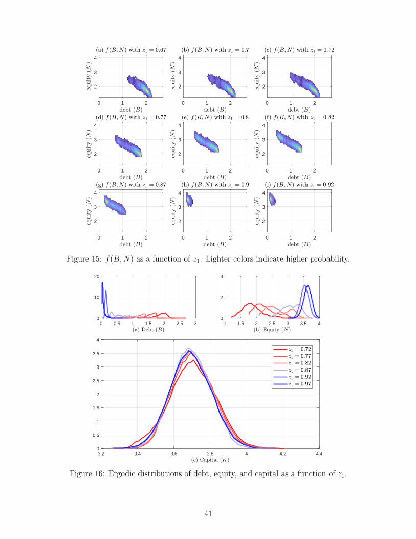
0 1 2

2

3

4

0 1 2

2

3

4

0 1 2

2

3

4

0 1 2

2

3

4

0 1 2

2

3

4

0 1 2

2

3

4

0 1 2

2

3

4

0 1 2

2

3

4

0 1 2

2

3

4

Figure 15: f(B,N) as a function of z1. Lighter colors indicate higher probability.

0 0.5 1 1.5 2 2.5 30

10

20

1 1.5 2 2.5 3 3.5 40

2

4

3.2 3.4 3.6 3.8 4 4.2 4.40

0.5

1

1.5

2

2.5

3

3.5

4

Figure 16: Ergodic distributions of debt, equity, and capital as a function of z1.

41

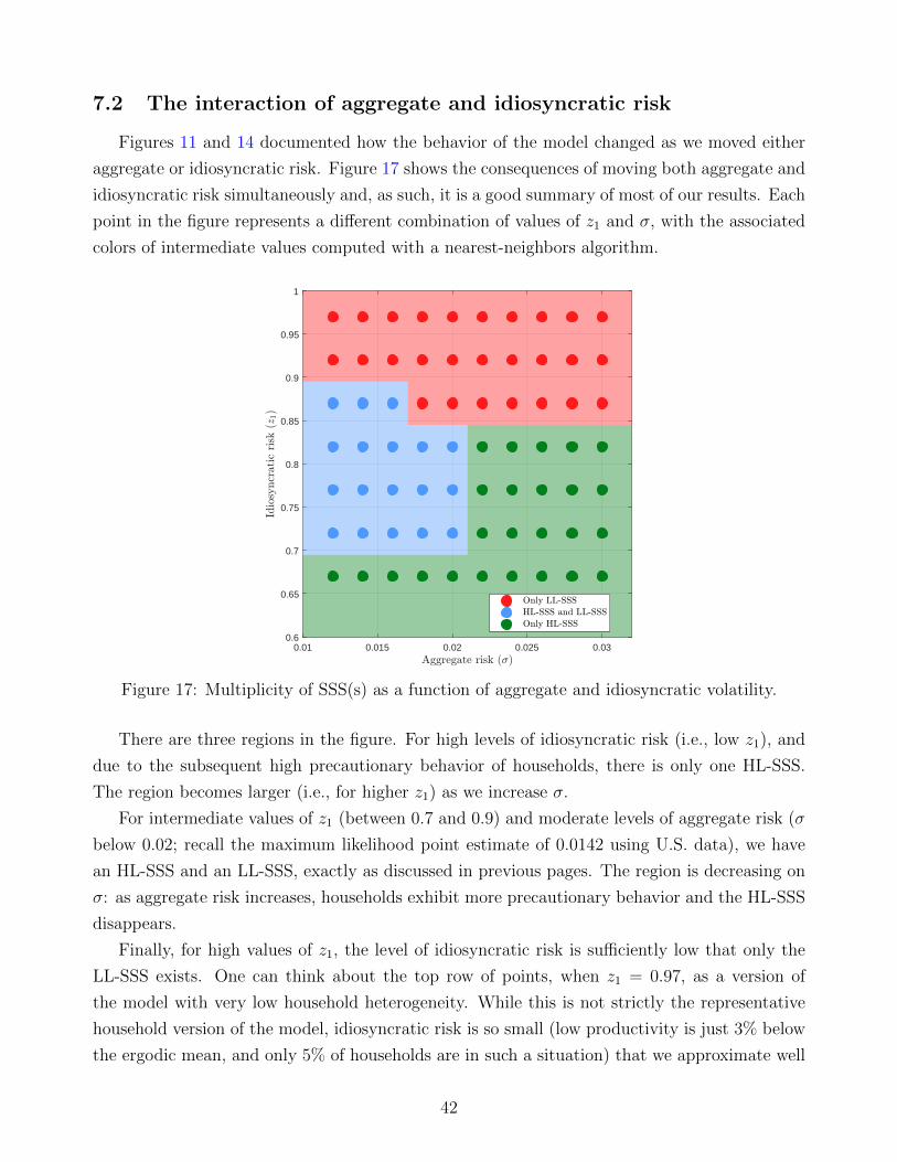
7.2 The interaction of aggregate and idiosyncratic risk

Figures 11 and 14 documented how the behavior of the model changed as we moved either

aggregate or idiosyncratic risk. Figure 17 shows the consequences of moving both aggregate and

idiosyncratic risk simultaneously and, as such, it is a good summary of most of our results. Each

point in the figure represents a different combination of values of z1 and σ, with the associated

colors of intermediate values computed with a nearest-neighbors algorithm.

0.01 0.015 0.02 0.025 0.030.6

0.65

0.7

0.75

0.8

0.85

0.9

0.95

1

Figure 17: Multiplicity of SSS(s) as a function of aggregate and idiosyncratic volatility.

There are three regions in the figure. For high levels of idiosyncratic risk (i.e., low z1), and

due to the subsequent high precautionary behavior of households, there is only one HL-SSS.

The region becomes larger (i.e., for higher z1) as we increase σ.

For intermediate values of z1 (between 0.7 and 0.9) and moderate levels of aggregate risk (σ

below 0.02; recall the maximum likelihood point estimate of 0.0142 using U.S. data), we have

an HL-SSS and an LL-SSS, exactly as discussed in previous pages. The region is decreasing on

σ: as aggregate risk increases, households exhibit more precautionary behavior and the HL-SSS

disappears.

Finally, for high values of z1, the level of idiosyncratic risk is sufficiently low that only the

LL-SSS exists. One can think about the top row of points, when z1 = 0.97, as a version of

the model with very low household heterogeneity. While this is not strictly the representative

household version of the model, idiosyncratic risk is so small (low productivity is just 3% below

the ergodic mean, and only 5% of households are in such a situation) that we approximate well

42

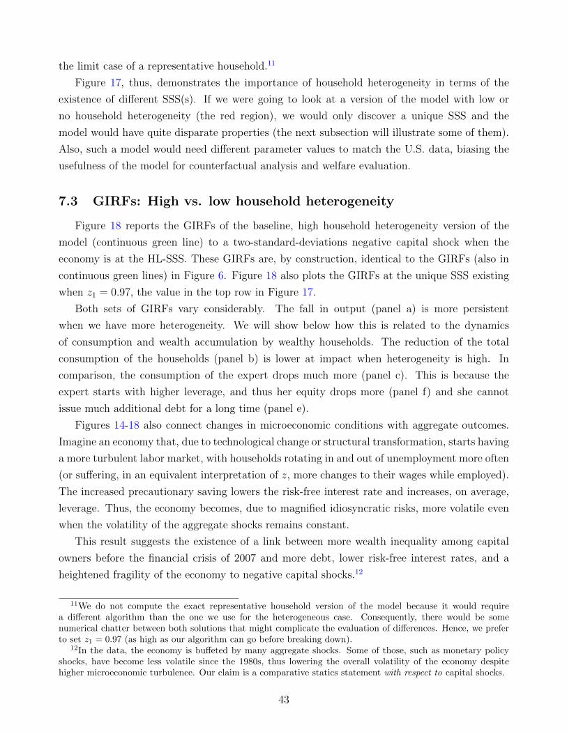
the limit case of a representative household.11

Figure 17, thus, demonstrates the importance of household heterogeneity in terms of the

existence of different SSS(s). If we were going to look at a version of the model with low or

no household heterogeneity (the red region), we would only discover a unique SSS and the

model would have quite disparate properties (the next subsection will illustrate some of them).

Also, such a model would need different parameter values to match the U.S. data, biasing the

usefulness of the model for counterfactual analysis and welfare evaluation.

7.3 GIRFs: High vs. low household heterogeneity

Figure 18 reports the GIRFs of the baseline, high household heterogeneity version of the

model (continuous green line) to a two-standard-deviations negative capital shock when the

economy is at the HL-SSS. These GIRFs are, by construction, identical to the GIRFs (also in

continuous green lines) in Figure 6. Figure 18 also plots the GIRFs at the unique SSS existing

when z1 = 0.97, the value in the top row in Figure 17.

Both sets of GIRFs vary considerably. The fall in output (panel a) is more persistent

when we have more heterogeneity. We will show below how this is related to the dynamics

of consumption and wealth accumulation by wealthy households. The reduction of the total

consumption of the households (panel b) is lower at impact when heterogeneity is high. In

comparison, the consumption of the expert drops much more (panel c). This is because the

expert starts with higher leverage, and thus her equity drops more (panel f) and she cannot

issue much additional debt for a long time (panel e).

Figures 14-18 also connect changes in microeconomic conditions with aggregate outcomes.

Imagine an economy that, due to technological change or structural transformation, starts having

a more turbulent labor market, with households rotating in and out of unemployment more often

(or suffering, in an equivalent interpretation of z, more changes to their wages while employed).

The increased precautionary saving lowers the risk-free interest rate and increases, on average,

leverage. Thus, the economy becomes, due to magnified idiosyncratic risks, more volatile even

when the volatility of the aggregate shocks remains constant.

This result suggests the existence of a link between more wealth inequality among capital

owners before the financial crisis of 2007 and more debt, lower risk-free interest rates, and a

heightened fragility of the economy to negative capital shocks.12

11We do not compute the exact representative household version of the model because it would requirea different algorithm than the one we use for the heterogeneous case. Consequently, there would be somenumerical chatter between both solutions that might complicate the evaluation of differences. Hence, we preferto set z1 = 0.97 (as high as our algorithm can go before breaking down).

12In the data, the economy is buffeted by many aggregate shocks. Some of those, such as monetary policyshocks, have become less volatile since the 1980s, thus lowering the overall volatility of the economy despitehigher microeconomic turbulence. Our claim is a comparative statics statement with respect to capital shocks.

43

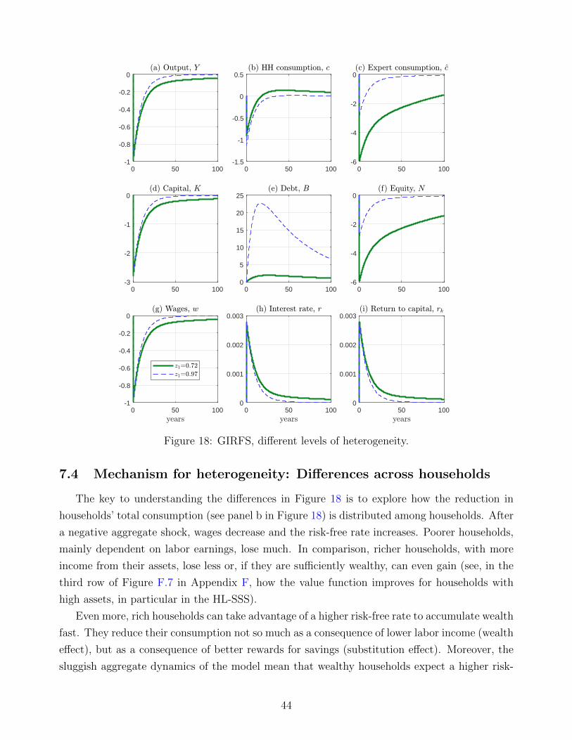
0 50 100-1

-0.8

-0.6

-0.4

-0.2

0

0 50 100-1.5

-1

-0.5

0

0.5

0 50 100-6

-4

-2

0

0 50 100-3

-2

-1

0

0 50 1000

5

10

15

20

25

0 50 100-6

-4

-2

0

0 50 100-1

-0.8

-0.6

-0.4

-0.2

0

0 50 1000

0.001

0.002

0.003

0 50 1000

0.001

0.002

0.003

Figure 18: GIRFS, different levels of heterogeneity.

7.4 Mechanism for heterogeneity: Differences across households

The key to understanding the differences in Figure 18 is to explore how the reduction in

households’ total consumption (see panel b in Figure 18) is distributed among households. After

a negative aggregate shock, wages decrease and the risk-free rate increases. Poorer households,

mainly dependent on labor earnings, lose much. In comparison, richer households, with more

income from their assets, lose less or, if they are sufficiently wealthy, can even gain (see, in the

third row of Figure F.7 in Appendix F, how the value function improves for households with

high assets, in particular in the HL-SSS).

Even more, rich households can take advantage of a higher risk-free rate to accumulate wealth

fast. They reduce their consumption not so much as a consequence of lower labor income (wealth

effect), but as a consequence of better rewards for savings (substitution effect). Moreover, the

sluggish aggregate dynamics of the model mean that wealthy households expect a higher risk-

44

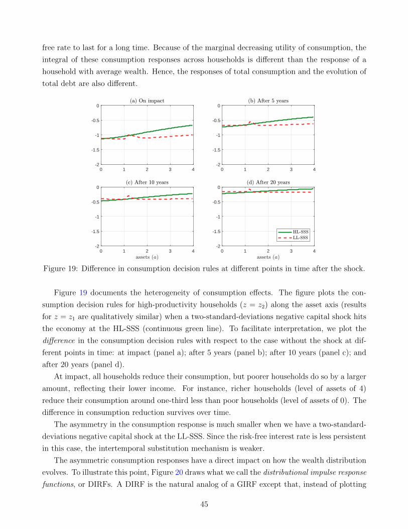
free rate to last for a long time. Because of the marginal decreasing utility of consumption, the

integral of these consumption responses across households is different than the response of a

household with average wealth. Hence, the responses of total consumption and the evolution of

total debt are also different.

0 1 2 3 4-2

-1.5

-1

-0.5

0

0 1 2 3 4-2

-1.5

-1

-0.5

0

0 1 2 3 4-2

-1.5

-1

-0.5

0

0 1 2 3 4-2

-1.5

-1

-0.5

0

Figure 19: Difference in consumption decision rules at different points in time after the shock.

Figure 19 documents the heterogeneity of consumption effects. The figure plots the con-

sumption decision rules for high-productivity households (z = z2) along the asset axis (results

for z = z1 are qualitatively similar) when a two-standard-deviations negative capital shock hits

the economy at the HL-SSS (continuous green line). To facilitate interpretation, we plot the

difference in the consumption decision rules with respect to the case without the shock at dif-

ferent points in time: at impact (panel a); after 5 years (panel b); after 10 years (panel c); and

after 20 years (panel d).

At impact, all households reduce their consumption, but poorer households do so by a larger

amount, reflecting their lower income. For instance, richer households (level of assets of 4)

reduce their consumption around one-third less than poor households (level of assets of 0). The

difference in consumption reduction survives over time.

The asymmetry in the consumption response is much smaller when we have a two-standard-

deviations negative capital shock at the LL-SSS. Since the risk-free interest rate is less persistent

in this case, the intertemporal substitution mechanism is weaker.

The asymmetric consumption responses have a direct impact on how the wealth distribution

evolves. To illustrate this point, Figure 20 draws what we call the distributional impulse response

functions, or DIRFs. A DIRF is the natural analog of a GIRF except that, instead of plotting

45

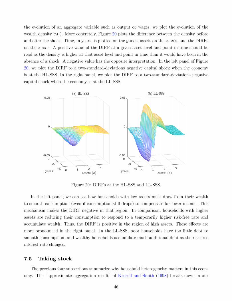
the evolution of an aggregate variable such as output or wages, we plot the evolution of the

wealth density gt(·). More concretely, Figure 20 plots the difference between the density before

and after the shock. Time, in years, is plotted on the y-axis, assets on the x-axis, and the DIRFs

on the z-axis. A positive value of the DIRF at a given asset level and point in time should be

read as the density is higher at that asset level and point in time than it would have been in the

absence of a shock. A negative value has the opposite interpretation. In the left panel of Figure

20, we plot the DIRF to a two-standard-deviations negative capital shock when the economy

is at the HL-SSS. In the right panel, we plot the DIRF to a two-standard-deviations negative

capital shock when the economy is at the LL-SSS.

-0.05

0

0

0.05

20

340 210

-0.05

0

0

0.05

20

340 210

Figure 20: DIRFs at the HL-SSS and LL-SSS.

In the left panel, we can see how households with low assets must draw from their wealth

to smooth consumption (even if consumption still drops) to compensate for lower income. This

mechanism makes the DIRF negative in that region. In comparison, households with higher

assets are reducing their consumption to respond to a temporarily higher risk-free rate and

accumulate wealth. Thus, the DIRF is positive in the region of high assets. These effects are

more pronounced in the right panel. In the LL-SSS, poor households have too little debt to

smooth consumption, and wealthy households accumulate much additional debt as the risk-free

interest rate changes.

7.5 Taking stock

The previous four subsections summarize why household heterogeneity matters in this econ-

omy. The “approximate aggregation result” of Krusell and Smith (1998) breaks down in our

46

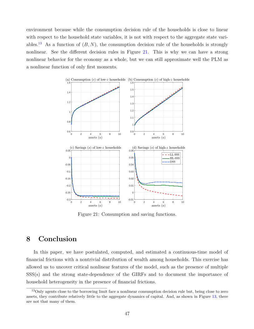
environment because while the consumption decision rule of the households is close to linear

with respect to the household state variables, it is not with respect to the aggregate state vari-

ables.13 As a function of (B,N), the consumption decision rule of the households is strongly

nonlinear. See the different decision rules in Figure 21. This is why we can have a strong

nonlinear behavior for the economy as a whole, but we can still approximate well the PLM as

a nonlinear function of only first moments.

0 2 4 6 8 100.6

0.8

1

1.2

1.4

1.6

0 2 4 6 8 100.9

1

1.1

1.2

1.3

1.4

1.5

1.6

0 2 4 6 8 10-0.3

-0.25

-0.2

-0.15

-0.1

-0.05

0

0.05

0 2 4 6 8 10-0.01

0

0.01

0.02

0.03

0.04

0.05

0.06

Figure 21: Consumption and saving functions.

8 Conclusion

In this paper, we have postulated, computed, and estimated a continuous-time model of

financial frictions with a nontrivial distribution of wealth among households. This exercise has

allowed us to uncover critical nonlinear features of the model, such as the presence of multiple

SSS(s) and the strong state-dependence of the GIRFs and to document the importance of

household heterogeneity in the presence of financial frictions.

13Only agents close to the borrowing limit face a nonlinear consumption decision rule but, being close to zeroassets, they contribute relatively little to the aggregate dynamics of capital. And, as shown in Figure 13, thereare not that many of them.

47

While we stand by the importance per se of our quantitative results, this paper can also be

understood as a “proof of concept” of how to efficiently compute and estimate a continuous-

time model with heterogeneous agents. For the computation, we have exploited tools borrowed

from machine learning. For the estimation, we have built on contributions from inference with

diffusions. The importance of heterogeneity for many questions in macroeconomics suggests that

there are multiple potential applications for the methodological tools that we presented and we

hope to show, in the near future, how to extend our current results to richer environments.

48

References

Achdou, Y., Han, J., Lasry, J.-M., Lions, P.-L., and Moll, B. (2017). Income and wealth

distribution in macroeconomics: A continuous-time approach. Working Paper 23732, National

Bureau of Economic Research.

Adrian, T. and Boyarchenko, N. (2012). Intermediary leverage cycles and financial stability.

Staff Report 567, Federal Reserve Bank of New York.

Adrian, T. and Shin, H. S. (2010). Liquidity and leverage. Journal of Financial Intermediation,

19(3):418–437.

Ahn, S., Kaplan, G., Moll, B., Winberry, T., and Wolf, C. (2017). When inequality matters for

macro and macro matters for inequality. In NBER Macroeconomics Annual 2017, Vol. 32.

University of Chicago Press.

Aıt-Sahalia, Y. (2002). Maximum likelihood estimation of discretely sampled diffusions: A

closed-form approximation approach. Econometrica, 70(1):223–262.

Aiyagari, S. R. (1994). Uninsured idiosyncratic risk and aggregate saving. Quarterly Journal of

Economics, 109(3):659–684.

Algan, Y., Allais, O., and Den Haan, W. J. (2008). Solving heterogeneous-agent models with

parameterized cross-sectional distributions. Journal of Economic Dynamics and Control,

32(3):875–908.

Algan, Y., Allais, O., Den Haan, W. J., and Rendahl, P. (2014). Solving and simulating models

with heterogeneous agents and aggregate uncertainty. In Schmedders, K. and Judd, K. L.,

editors, Handbook of Computational Economics, volume 3, pages 277–324. Elsevier.

Alvaredo, F., Chancel, L., Piketty, T., Saez, E., and Zucman, G. (2017). Global inequality

dynamics: New findings from wid.world. Working Paper 23119, National Bureau of Economic

Research.

Andersen, T. G. and Lund, J. (1997). Estimating continuous-time stochastic volatility models

of the short-term interest rate. Journal of Econometrics, 77(2):343–377.

Auclert, A. (2016). Monetary policy and the redistribution channel. Stanford University.

Auclert, A., Bardoczy, B., Rognlie, M., and Straub, L. (2019). Using the sequence-space Jacobian

to solve and estimate heterogeneous-agent models. Mimeo, Stanford University.

Auclert, A. and Rognlie, M. (2018). Inequality and aggregate demand. Stanford University.

49

Bach, F. (2017). Breaking the curse of dimensionality with convex neural networks. Journal of

Machine Learning Research, 18(1):629–681.

Barron, A. R. (1993). Universal approximation bounds for superpositions of a sigmoidal function.

IEEE Transactions on Information Theory, 39(3):930–945.

Barucci, E. and Landi, L. (1995). Non-parametric versus linear learning devices: A procedural

perspective. Technical report, University of Florence.

Basak, S. and Cuoco, D. (1998). An equilibrium model with restricted stock market participa-

tion. Review of Financial Studies, 11(2):309–341.

Bayer, C. and Luetticke, R. (2018). Solving heterogeneous agent models in discrete time with

many idiosyncratic states by perturbation methods. Mimeo, University of Bonn.

Bergin, J. and Bernhardt, D. (1992). Anonymous sequential games with aggregate uncertainty.

Journal of Mathematical Economics, 21(6):543–562.

Bernanke, B. S., Gertler, M., and Gilchrist, S. (1999). The financial accelerator in a quanti-

tative business cycle framework. In Taylor, J. B. and Woodford, M., editors, Handbook of

Macroeconomics, volume 1, pages 1341–1393. Elsevier.

Bishop, C. M. (2006). Pattern Recognition and Machine Learning. Springer-Verlag.

Blanchard, O. and Galı, J. (2010). Labor markets and monetary policy: A New Keynesian

model with unemployment. American Economic Journal: Macroeconomics, 2(2):1–30.

Brunnermeier, M. K. and Sannikov, Y. (2014). A macroeconomic model with a financial sector.

American Economic Review, 104(2):379–421.

Candler, G. V. (1999). Finite difference methods for continuous time dynamic programming.

In Marimon, R. and Scott, A., editors, Computational Methods for the Study of Dynamic

Economies, pages 172–194. Oxford University Press.

Chacko, G. and Viceira, L. M. (2003). Spectral GMM estimation of continuous-time processes.

Journal of Econometrics, 116(1):259–292.

Cho, I.-K. (1995). Perceptrons play the repeated prisoner’s dilemma. Journal of Economic

Theory, 67(1):266–284.

Cho, I.-K. and Sargent, T. J. (1996). Neural networks for encoding and adapting in dynamic

economies. In Amman, H., Kendrick, D., and Rust, J., editors, Handbook of Computational

Economics, volume 1, pages 441–470. Elsevier.

50

Cybenko, G. (1989). Approximation by superpositions of a sigmoidal function. Mathematics of

Control, Signals and Systems, 2(4):303–314.

Den Haan, W. J. (1996). Heterogeneity, aggregate uncertainty, and the short-term interest rate.

Journal of Business & Economic Statistics, 14(4):399–411.

Den Haan, W. J. (1997). Solving dynamic models with aggregate shocks and heterogeneous

agents. Macroeconomic Dynamics, 1(02):355–386.

Den Haan, W. J. and Rendahl, P. (2010). Solving the incomplete markets model with aggregate

uncertainty using explicit aggregation. Journal of Economic Dynamics and Control, 34(1):69–

78.

Duarte, V. (2018). Sectoral reallocation and endogenous risk-aversion: Solving macro-finance

models with machine learning. MIT Sloan School of Management.

Duffie, D. and Epstein, L. (1992). Stochastic differential utility. Econometrica, 60(2):353–94.

Evans, G. W. and Honkapohja, S. (2001). Learning and Expectations in Macroeconomics. Prince-

ton University Press.

Fernandez-Villaverde, J. and Rubio-Ramırez, J. F. (2007). Estimating macroeconomic models:

A likelihood approach. Review of Economic Studies, 74(4):1059–1087.

Galı, J. and Gambetti, L. (2009). On the sources of the Great Moderation. American Economic

Journal: Macroeconomics, 1(1):26–57.

Goodfellow, I., Bengio, Y., and Courville, A. (2016). Deep Learning. MIT Press. http:

//www.deeplearningbook.org.

Gornemann, N., Kuester, K., and Nakajima, M. (2012). Monetary policy with heterogeneous

agents. Working Paper 12-21, Federal Reserve Bank of Philadelphia.

Hall, R. E. and Milgrom, P. R. (2008). The limited influence of unemployment on the wage

bargain. American Economic Review, 98(4):1653–74.

He, Z. and Krishnamurthy, A. (2012). A model of capital and crises. Review of Economic

Studies, 79(2):735–777.

He, Z. and Krishnamurthy, A. (2013). Intermediary asset pricing. American Economic Review,

103(2):732–70.

Holston, K., Laubach, T., and Williams, J. C. (2017). Measuring the natural rate of interest:

International trends and determinants. Journal of International Economics, 108:S59 – S75.

51

Hornik, K., Stinchcombe, M., and White, H. (1989). Multilayer feedforward networks are

universal approximators. Neural Networks, 2(5):359–366.

Huggett, M. (1993). The risk-free rate in heterogeneous-agent incomplete-insurance economies.

Journal of Economic Dynamics and Control, 17(5-6):953–969.

Kaplan, G., Moll, B., and Violante, G. L. (2018). Monetary policy according to HANK. Amer-

ican Economic Review, 108(3):697–743.

Kiyotaki, N. and Moore, J. (1997). Credit cycles. Journal of Political Economy, 105(2):211–248.

Krusell, P. and Smith, A. A. (1998). Income and wealth heterogeneity in the macroeconomy.

Journal of Political Economy, 106(5):867–896.

Kubler, F. and Scheidegger, S. (2018). Self-justified equilibria: Existence and computation.

Working Paper, DBF, University of Zurich.

Kumhof, M., Ranciere, R., and Winant, P. (2015). Inequality, leverage, and crises. American

Economic Review, 105(3):1217–45.

Liu, P., Theodoridis, K., Mumtaz, H., and Zanetti, F. (2018). Changing macroeconomic dy-

namics at the zero lower bound. Journal of Business & Economic Statistics, 0(0):1–14.

Lo, A. (1988). Maximum likelihood estimation of generalized Ito processes with discretely

sampled data. Econometric Theory, 4(2):231–247.

Luetticke, R. (2015). Transmission of monetary policy and heterogeneity in household portfolios.

UCL.

Maliar, L., Maliar, S., and Valli, F. (2010). Solving the incomplete markets model with aggregate

uncertainty using the Krusell-Smith algorithm. Journal of Economic Dynamics and Control,

34(1):42–49.

McKay, A., Nakamura, E., and Steinsson, J. (2016). The power of forward guidance revisited.

American Economic Review, 106(10):3133–58.

Miao, J. (2006). Competitive equilibria of economies with a continuum of consumers and ag-

gregate shocks. Journal of Economic Theory, 128(1):274–298.

Nuno, G. and Thomas, C. (2016). Optimal monetary policy with heterogeneous agents. Working

Paper 1624, Banco de Espana.

Nuno, G. and Thomas, C. (2017). Bank leverage cycles. American Economic Journal: Macroe-

conomics, 9(2):32–72.

52

Prohl, E. (2015). Approximating equilibria with ex-post heterogeneity and aggregate risk. Re-

search Paper 17-63, Swiss Finance Institute.

Reiter, M. (2009). Solving heterogeneous-agent models by projection and perturbation. Journal

of Economic Dynamics and Control, 33(3):649–665.

Reiter, M. (2010). Solving the incomplete markets model with aggregate uncertainty by back-

ward induction. Journal of Economic Dynamics and Control, 34(1):28–35.

Rıos-Rull, J.-V. (1997). Computation of equilibria in heterogeneous agent models. Staff Report

231, Federal Reserve Bank of Minneapolis.

Rumelhart, D. E., Hinton, G. E., and Williams, R. J. (1986). Learning representations by

back-propagating errors. Nature, 323:533–536.

Sager, E. (2014). Solving the incomplete markets model with aggregate uncertainty: The method

of mixtures. Bureau of Labor Statistics, Price Research Division.

Salmon, M. (1995). Bounded rationality and learning: Procedural learning. In Kirman, A. P.

and Salmon, M., editors, Learning and Rationality in Economics, pages 236–275. Blackwell

Publishing.

Scheidegger, S. and Bilionis, I. (2017). Machine learning for high-dimensional dynamic stochastic

economies. UCL.

Young, E. R. (2010). Solving the incomplete markets model with aggregate uncertainty using

the Krusell-Smith algorithm and non-stochastic simulations. Journal of Economic Dynamics

and Control, 34(1):36–41.

53

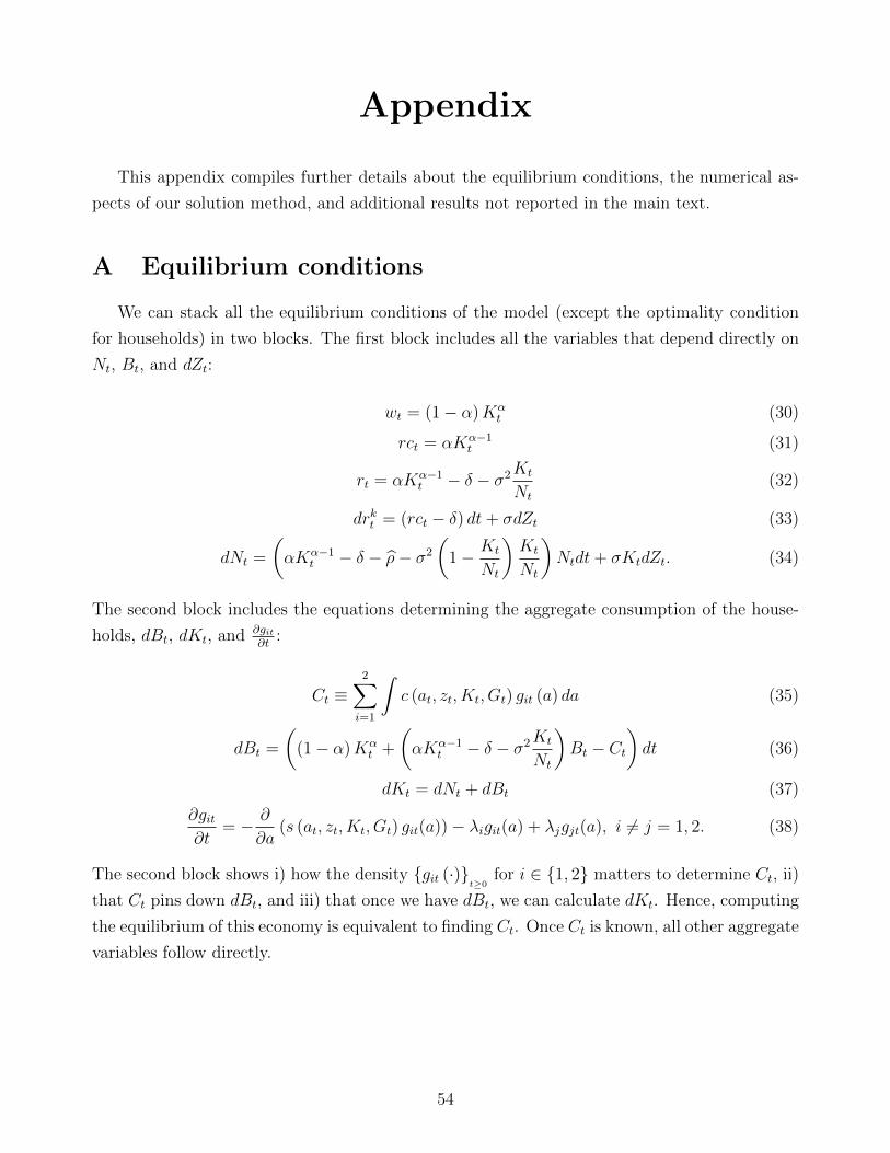
Appendix

This appendix compiles further details about the equilibrium conditions, the numerical as-

pects of our solution method, and additional results not reported in the main text.

A Equilibrium conditions

We can stack all the equilibrium conditions of the model (except the optimality condition

for households) in two blocks. The first block includes all the variables that depend directly on

Nt, Bt, and dZt:

wt = (1− α)Kαt (30)

rct = αKα−1t (31)

rt = αKα−1t − δ − σ2Kt

Nt

(32)

drkt = (rct − δ) dt+ σdZt (33)

dNt =

(αKα−1

t − δ − ρ− σ2

(1− Kt

Nt

)Kt

Nt

)Ntdt+ σKtdZt. (34)

The second block includes the equations determining the aggregate consumption of the house-

holds, dBt, dKt, and ∂git∂t

:

Ct ≡2∑i=1

∫c (at, zt, Kt, Gt) git (a) da (35)

dBt =

((1− α)Kα

t +

(αKα−1

t − δ − σ2Kt

Nt

)Bt − Ct

)dt (36)

dKt = dNt + dBt (37)

∂git∂t

= − ∂

∂a(s (at, zt, Kt, Gt) git(a))− λigit(a) + λjgjt(a), i 6= j = 1, 2. (38)

The second block shows i) how the density git (·)t≥0

for i ∈ 1, 2 matters to determine Ct, ii)

that Ct pins down dBt, and iii) that once we have dBt, we can calculate dKt. Hence, computing

the equilibrium of this economy is equivalent to finding Ct. Once Ct is known, all other aggregate

variables follow directly.

54

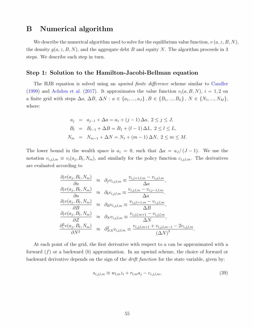
B Numerical algorithm

We describe the numerical algorithm used to solve for the equilibrium value function, v (a, z, B,N),

the density g(a, z, B,N), and the aggregate debt B and equity N . The algorithm proceeds in 3

steps. We describe each step in turn.

Step 1: Solution to the Hamilton-Jacobi-Bellman equation

The HJB equation is solved using an upwind finite difference scheme similar to Candler

(1999) and Achdou et al. (2017). It approximates the value function vi(a,B,N), i = 1, 2 on

a finite grid with steps ∆a, ∆B, ∆N : a ∈ a1, ..., aJ , B ∈ B1, ..., BL , N ∈ N1, ..., NM,where:

aj = aj−1 + ∆a = a1 + (j − 1) ∆a, 2 ≤ j ≤ J,

Bl = Bl−1 + ∆B = B1 + (l − 1) ∆L, 2 ≤ l ≤ L,

Nm = Nm−1 + ∆N = N1 + (m− 1) ∆N, 2 ≤ m ≤M.

The lower bound in the wealth space is a1 = 0, such that ∆a = aJ/ (J − 1). We use the

notation vi,j,l,m ≡ vi(aj, Bl, Nm), and similarly for the policy function ci,j,l,m. The derivatives

are evaluated according to

∂iv(aj, Bl, Nm)

∂a≈ ∂fvi,j,l,m ≡

vi,j+1,l,m − vi,j,l,m∆a

,

∂iv(aj, Bl, Nm)

∂a≈ ∂bvi,j,l,m ≡

vi,j,l,m − vi,j−1,l,m

∆a.

∂iv(aj, Bl, Nm)

∂B≈ ∂Bvi,j,l,m ≡

vi,j,l+1,m − vi,j,l,m∆B

,

∂iv(aj, Bl, Nm)

∂Z≈ ∂Nvi,j,l,m ≡

vi,j,l,m+1 − vi,j,l,m∆N

,

∂2i v(aj, Bl, Nm)

∂N2≈ ∂2

NNvi,j,l,m ≡vi,j,l,m+1 + vi,j,l,m−1 − 2vi,j,l,m

(∆N)2 .

At each point of the grid, the first derivative with respect to a can be approximated with a

forward (f) or a backward (b) approximation. In an upwind scheme, the choice of forward or

backward derivative depends on the sign of the drift function for the state variable, given by:

si,j,l,m ≡ wl,mzi + rl,maj − ci,j,l,m, (39)

55

where:

ci,j,l,m =

[∂vi,j,l,m∂a

]−1/γ

, (40)

wl,m = (1− α)Z (Bl +Nm)α , (41)

rl,m = αZ (Bl +Nm)α−1 − δ − σ2 (Bl +Nm)

Nm

. (42)

Let superscript n denote the iteration counter. The HJB equation is approximated by the

following upwind scheme:

vn+1i,j,l,m − vni,j,l,m

∆+ ρvn+1

i,j,l,m =(cni,j,l,m)1−γ − 1

1− γ+ ∂fv

n+1i,j,l,ms

ni,j,l,m,f1sni,j,n,m,f>0 + ∂Bv

n+1i,j,l,ms

ni,j,l,m,b1sni,j,l,m,b<0

+λi(vn+1−i,j,l,m − v

n+1i,j,l,m

)+ hl,m∂Bvi,j,l,m + µNl,m∂Nvi,j,l,m

+

[σNl,m

]22

∂2NNvi,j,l,m

for i = 1, 2, j = 1, ..., J , l = 1, .., L, m = 1, ...,M , where 1 (·) is the indicator function and

hl,m ≡ h (Bl, Nm) ,

µNl,m ≡ µN (Bl, Nm) = αZ (Bl +Nm)α − δ (Bl +Nm)− rl,mBl − ρNm,

σNl,m ≡ σN (Bl, Nm) = σ (Bl +Nm) ,

sni,j,l,m,f = wl,mzi + rl,maj −

[1

∂nf vi,j,l,m

]1/γ

,

sni,j,l,m,b = wl,mzi + rl,maj −[

1

∂nb vi,j,l,m

]1/γ

.

Thus, when the drift is positive (sni,j,l,m,f > 0), we employ a forward approximation of the

derivative, ∂nf vi,j,l,m; when it is negative (sni,j,l,m,b < 0), we employ a backward approximation,

∂nb vi,j,l,m. The termvn+1i,j,l,m−v

ni,j,l,m

∆→ 0 as vn+1

i,j,l,m → vni,j,l,m.

Moving all terms involving vn+1 to the left-hand side and the rest to the right-hand side, we

obtain:

vn+1i,j,l,m − vni,j,l,m

∆+ ρvn+1

i,j,l,m =(cni,j,n,m)1−γ − 1

1− γ+ vn+1

i,j−1,l,mαni,j,l,m + vn+1

i,j,l,mβni,j,l,m + vn+1

i,j+1,l,mξni,j,l,m

+λivn+1−i,j,l,m + vn+1

i,j,l+1,m

hl,m∆B

+ vn+1i,j,l,m+1κl,m + vn+1

i,j,l,m−1%l,m (43)

56

where:

αni,j ≡ −sni,j,B1sni,j,B<0

∆a,

βni,j,l,m ≡ −sni,j,l,m,f1sni,j,n,mF>0

∆a+sni,j,l,m,b1sni,j,l,m,b<0

∆a− λi −

hl,m∆B−µNl,m∆N

−(σNl,m

)2

(∆N)2 ,

ξni,j ≡sni,j,F1sni,j,F>0

∆a,

κl,m ≡µNl,m∆N

+

(σNl,m

)2

2 (∆N)2 =[αZ (Bl +Nm)α − δ (Bl +Nm)− rl,mBl − ρNm]

∆N+σ2 (Bl +Nm)2

2 (∆N)2 ,

%l,m ≡(σNl,m

)2

2 (∆N)2 =σ2 (Bl +Nm)2

2 (∆N)2 .

for i = 1, 2, j = 1, ..., J , l = 1, .., L, m = 1, ...,M . We consider boundary state constraints in a

(sni,1,B = sni,J,F = 0). The boundary conditions in B and N are reflections.

In equation (43), the optimal consumption is set to:

cni,j,n,m =(∂vni,j,l,m

)−1/γ. (44)

where:

∂vni,j,l,m = ∂fvni,j,l,m1sni,j,n,mF>0 + ∂bv

ni,j,l,m1sni,j,l,m,b<0 + ∂vni,j,l,m1sni,j,n,mF≤01sni,j,l,m,b≥0.

In the above expression, ∂vni,j,l,m = (cni,j,n,m)−γ where cni,j,n,m is the consumption level such that

the drift is zero:

cni,j = wl,mzi + rl,maj.

57

We define:

Anl.m =

βn1,1,l,m ξn1,1,l,m 0 0 · · · 0 λ1 0 · · · 0

αn1,2,l,m βn1,2,l,m ξn1,2,l,m 0 · · · 0 0 λ1. . . 0

0 αn1,3,l,m βn1,3,l,m ξn1,3,l,m · · · 0 0 0. . .

......

. . . . . . . . . . . . . . . . . . . . . . . ....

0 0 · · · αn1,J−1,l,m βn1,J−1,l,m ξn1,J−1,l,m 0 · · · λ1 0

0 0 · · · 0 αn1,J,l,m βn1,J,l,m 0 0 · · · λ1

λ2 0 · · · 0 0 0 βn2,1,l,m ξn2,1,l,m · · · 0...

. . . . . . . . . . . . . . ....

. . . . . ....

0 0 · · · 0 0 λ2 0 · · · αn2,J,l,m βn2,J,l,m

,

vn+1l,m =

vn+11,1,l,m

vn+11,2,l,m

...

vn+11,J,l,m

vn+12,1,l,m

...

vn+12,J,l,m

and

Anm =

An1,m

h1,m

∆KI2J 02J · · · 02J 02J

02J An2,m

h2,m

∆KI2J · · · 02J 02J

02J 02J An3,m · · · 02J 02J

.... . . . . . . . . . . .

...

02J AnL−1,m

hL−1,m

∆KI2J

02J 02J · · · 02J 02J

(AnL,m +

hL,m∆K

I2J

)

, vn+1

m =

vn+1

1,m

vn+12,m...

vn+1L,m

,

where In and 0n are the identity matrix and the zero matrix of dimension n × n, respectively.

58

We can also define

An =

(An1 + P1) X1 02J×L · · · 02J×L 02J×L

P2 An2 X2 · · · 02J×L 02J×L

02J×L P3 An3 · · · 02J×L 02J×L

.... . . . . . . . . . . .

...

PM−1 AnM−1 XM−1

02J×L 02J×L · · · 02J×L PM (AnM + XM)

, vn+1 =

vn+1

1

vn+12...

vn+1M

,

Xm =

κ1,mI2J 02J · · · 02J 02J

02J κ2,mI2J · · · 02J 02J

.... . . . . . . . .

...

02J κL−1,mI2J 02J

02J 02J 02J 02J κL,mI2J

,

Pm =

%1,mI2J 02J · · · 02J 02J

02J %2,mI2J · · · 02J 02J

.... . . . . . . . .

...

02J %L−1,mI2J 02J

02J 02J 02J 02J %L,mI2J

,un =

(cn1,1,1,1)1−γ−1

1−γ(cn1,2,1,1)1−γ−1

1−γ......

(cn2,J,L,M )1−γ−1

1−γ

.

Then, equation (43) is a system of 2×J ×L×M linear equations that can be written in matrix

notation as:1

∆

(vn+1 − vn

)+ ρvn+1 = un + Anvn+1.

The system in turn can be written as

Bnvn+1 = dn (45)

where Bn =(

1∆

+ ρ)I−An and dn = un + 1

∆vn.

The algorithm to solve the HJB equation begins with an initial guess v0i,j,l,m. Set n = 0.

Then:

1. Compute cni,j,l,m, i = 1, 2 using (44).

2. Find vn+1i,j,l,m solving the linear system of equations (45).

3. If vn+1i,j,l,m is close enough to vni,j,l,m, stop. If not, set n := n+ 1 and proceed to step 1.

Most programming languages, such as Julia or Matlab, include efficient routines to handle

sparse matrices such as An.

59

Step 2: Solution to the KF equation

The income-wealth distribution conditional on the current realization of aggregate debt

B = Bl and equity N = Nm can be characterized by the KF equation:

∂g

∂t= − ∂

∂a[si (a,B,N) gi,t(a)]− λigi,t(a) + λ−ig−i,t(a), i = 1, 2. (46)

1 =

∫ ∞0

g(a)da. (47)

If we define a time step ∆t, we also solve this equation using an finite difference scheme. We

use the notation gi,j ≡ gi(aj). The system can be now expressed as:

gi,j,t+1 − gi,j∆t

= −gi,j,tsi,j,l,m,b1si,j,l,m,b>0 − gi,j−1,tsi,j−1,l,m,f1si,j−1,l,m,f>0

∆a

−gi,j+1,tsi,j+1,l,m,b1si,j+1,l,m,b<0 − gi,j,tsi,j,l,m,b1si,j,l,m,b<0

∆a− λigi,j,t + λ−ig−i,j,t.

In this case, let us define

gt =

g1,1,t

g1,2,t

...

g1,J,t

g2,1,t

...

g2,J,t

,

as the density conditional on the current state of Bl and Nm. We assume that g0 is the density

in the DSS, and the update in the next time period is given by the KF equation:

gt+1 =(I−∆tAT

l,m

)−1gt,

where ATl,m is the transpose matrix of Al,m = limn→∞An

l,m, defined above.

Step 3: Update of the PLM using a neural network

The vector θ is recursively updated according to θm+1 = θm − εm∇E(θ; sj, hj

), where:

∇E(θ; sj, hj

)≡

∂E(θ; sj, hj

)∂θ2

0

,∂E(θ; sj, hj

)∂θ2

1

, ...,∂E(θ; sj, hj

)∂θ1

2,Q

>

60

is the gradient of the error function with respect to θ evaluated at(sj, hj

).

The step size εm > 0 is selected in each iteration according to a line-search algorithm in

order to minimize the error function in the direction of the gradient. The algorithm is run until

‖θm+1 − θm‖ < ε, for a small ε.

The error gradient can be efficiently evaluated using a back-propagation algorithm, originally

developed by Rumelhart et al. (1986), which builds on the chain rule of differential calculus. In

our case, the corresponding formulae are:

∂E(θ; sj, hj

)∂θ2

0

= h (sj; θ)− hj

∂E(θ; sj, hj

)∂θ2

q

=(h (sj; θ)− hj

)φ

(θ1

0,q +2∑i=1

θ1i,qs

ij

), for q = 1, ..., Q

∂E(θ; sj, hj

)∂θ1

0,q

= θ2q

(h (sj; θ)− hj

)φ′

(θ1

0,q +2∑i=1

θ1i,qs

ij

), for q = 1, ..., Q

∂E(θ; sj, hj

)∂θ1

i,q

= sijθ2q

(h (sj; θ)− hj

)φ′

(θ1

0,q +2∑i=1

θ1i,qs

ij

), for i = 1, 2 and q = 1, ..., Q,

where φ′(x) = 1(1+e−x)

.

We fine-tune the training scheme of our neural network in several ways to meet the specific

demands of the problem at hand.

First, the training scheme needs to yield a consistently good approximation: a “not-good-

enough” approximation in any of the dozens of iterations of the algorithm can make it break

and not deliver a result. This is the reason we employ a line-search instead of using a constant

or adaptive learning rate: it prevents bad steps in the minimization.

Second, the training scheme cannot introduce big amounts of noise in the progressive ap-

proximation to the solution of the model. Otherwise, the noise can mask or prevent convergence

(strict convergence criteria can only be met by chance, if at all). This is why we use a batch

gradient descent (i.e., all training points are used in every gradient calculation and line-search

step) instead of the more popular stochastic or mini-batch gradient descents. The random choice

of training points in each step, common in the machine learning literature, would make progress

stochastic and introduces noise.

Reducing stochastic elements in the solution method is also why we train the model with a

grid approximation that clears out noise. We define a 101x101 grid over the (B,N) support, and

assign each simulated point to one of the knots in that grid. Then, we run a linear regression,

and use it to estimate the height of the PLM at that knot. This grid could later be used to

solve the model using interpolation (e.g., with splines, or with natural neighbor interpolation)

61

and linear extrapolation (and we do that as a robustness check, finding similar results to those

of the solution with the neural network). However, on a 2D surface. such extrapolation tends

to generate ridges (because of the amplification of sample noise in far-away extrapolations),

which could prevent convergence at the HJB step. Instead, we use those knots to train the

neural network, which provides a good-enough fit in the visited area and a much smoother

extrapolation to the nonvisited area of the (B,N) support.

Finally, the need to avoid stochastic elements that introduce noise in the algorithm, plus a

desire for fast running times, made us change the usual Monte Carlo multi-start initialization

of the neural network parameters for all iterations except the first one. In the first iteration of

the algorithm, we do ten random initializations of the parameters of the neural network and ten

subsequent training sessions. Later, we choose the best-performing trained network across those

ten training sessions. From the second iteration onwards, the neural network is initialized using

weights that were found to be optimal in the previous iteration, and a single training session

is carried out. This avoids re-introducing a stochastic element on each step of the algorithm.

Using a small relaxation parameter in the PLM update step (it starts at 0.30 and exponentially

decays towards 0.05, reaching 0.20 after five iterations and 0.10 after 16) makes the convergence

of the full algorithm slower but smoother, with slow updates to the optimal neural network that

help this non-random initialization work well.

Notice, however, that since we are interested in approximating an unknown function, not

clearing a market or satisfying an optimality condition, local minima that are close to a global

minimum are often acceptable solutions to the approximation problem.

Complete algorithm

We can now summarize the complete algorithm. We begin a guess of the PLM h0 (B,N).

Set s := 1 :

Step 1: Household problem. Given hs−1 (B,N) , solve the HJB equation to obtain an esti-

mate of the value function v and of the matrix A.

Step 2: Distribution. Given A, simulate T periods of the economy using the KF equation

and obtain the aggregated ebt BtTt=0 and equity NtTt=0 . The law of motion of equity is

Nt = Nt−1 + [αZ (Bt +Nt)α − δ (Bt +Nt)− rtBt − ρNt] ∆t+ σ (Bt +Nt)

√∆tεt,

where εtiid∼ N(0, 1).

Step 3: PLM. Update the PLM using a neural netwok: hs. If ‖hs − hs−1‖ < ε, where ε is a

small positive constant, then stop. If not, return to step 1.

62

C Evaluating the likelihood function with micro obser-

vations

A promising avenue to improve the estimation in the main text is to add micro observations,

which bring much additional information and help in integrating different levels of aggregation

to assess the empirical validity of the model. More concretely, let Xt ≡ [gt(a, z);Nt]′ be a vector

of observations on the asset holdings of agents in this economy (households, gt(a, z), and the

expert, Nt). Imagine, as before, that we have D + 1 observations of Xt at fixed time intervals

[0,∆, 2∆, .., D∆, ]:

XD0 = X0, X∆, X2∆, ..., XD .

At this moment, we need to assume –as is typically done in models with heterogeneous agents

and aggregates shocks– that the conditional no aggregate uncertainty (CNAU) condition holds.

See, for instance, Miao (2006), following Bergin and Bernhardt (1992). This condition implies

that if households are distributed on the interval I = [0, 1] according to the Lebesgue measure

Φ, then

Gt(A× Z) = Φ(i ∈ I :

(ait, z

it

)∈ A× Z

),

for any subsets A ⊂ [0,∞), Z ⊂ z1, z2. That is, the probability under the conditional

distribution is the same as the probability according to the Lebesgue measure across I.

The likekihood that an individual agent i ∈ I at time t = d∆ is at state (aid∆, zid∆, Bd∆, Nd∆)

is fdd∆(aid∆, zid∆, Bd∆, Nd∆). The log-likelihood is then log

[fdd∆(aid∆, z

id∆, Bd∆, Nd∆)

]. Notice that

this log-likelihood is a function of i.

The conditional aggregate log-likelihood across all agents is:

log pX(Xd∆|X(d−1)∆; Ψ

)=

∫log[fdd∆(aid∆, z

id∆, Bd∆, Nd∆)

]Φ(di),

and, taking into account the CNAU condition, we get:∫log[fdd∆(aid∆, z

id∆, Bd∆, Nd∆)

]Φ(di) =

∫log[fdd∆(a, z, Bd∆, Nd∆)

]Gd∆(da, dz)

=2∑i=1

∫ ∞0

log[fdd∆(a, zi, Bd∆, Nd∆)

]gd∆(a, z)da,

where, in the second line, we have applied the definition of the Radon-Nikodym derivative to

get the differential in a.

63

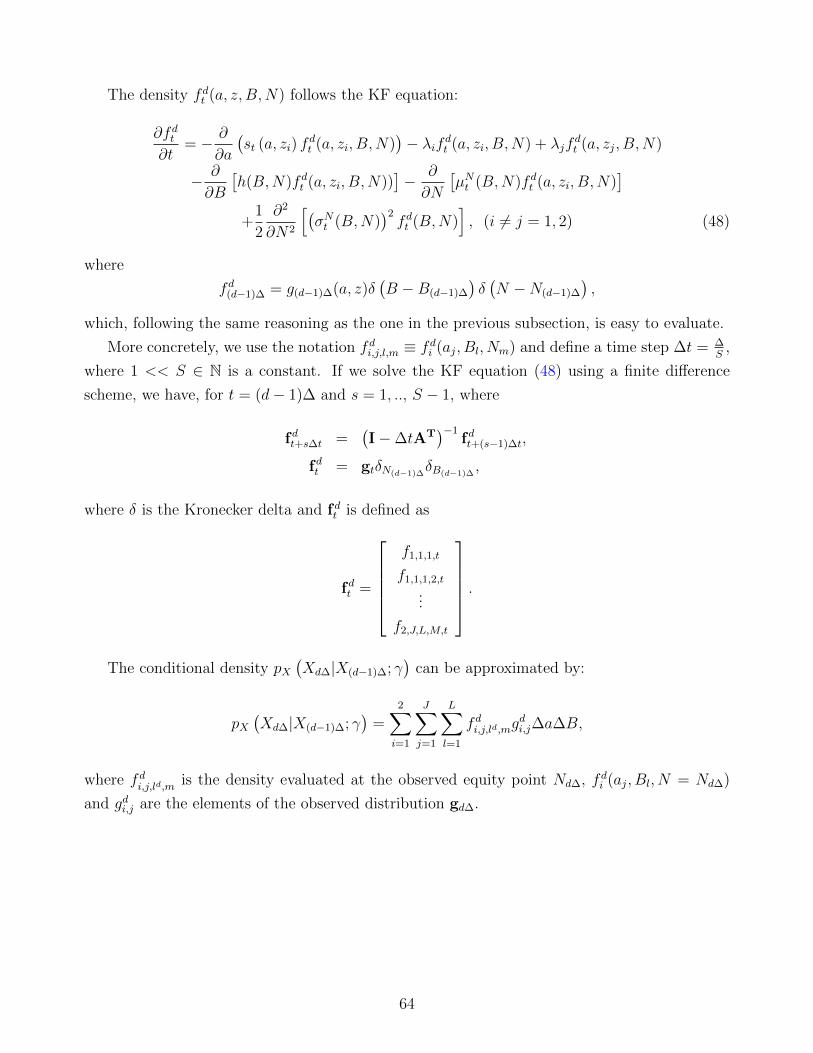
The density fdt (a, z, B,N) follows the KF equation:

∂fdt∂t

= − ∂

∂a

(st (a, zi) f

dt (a, zi, B,N)

)− λifdt (a, zi, B,N) + λjf

dt (a, zj, B,N)

− ∂

∂B

[h(B,N)fdt (a, zi, B,N))

]− ∂

∂N

[µNt (B,N)fdt (a, zi, B,N)

]+

1

2

∂2

∂N2

[(σNt (B,N)

)2fdt (B,N)

], (i 6= j = 1, 2) (48)

where

fd(d−1)∆ = g(d−1)∆(a, z)δ(B −B(d−1)∆

)δ(N −N(d−1)∆

),

which, following the same reasoning as the one in the previous subsection, is easy to evaluate.

More concretely, we use the notation fdi,j,l,m ≡ fdi (aj, Bl, Nm) and define a time step ∆t = ∆S,

where 1 << S ∈ N is a constant. If we solve the KF equation (48) using a finite difference

scheme, we have, for t = (d− 1)∆ and s = 1, .., S − 1, where

fdt+s∆t =(I−∆tAT

)−1fdt+(s−1)∆t,

fdt = gtδN(d−1)∆δB(d−1)∆

,

where δ is the Kronecker delta and fdt is defined as

fdt =

f1,1,1,t

f1,1,1,2,t

...

f2,J,L,M,t

.

The conditional density pX(Xd∆|X(d−1)∆; γ

)can be approximated by:

pX(Xd∆|X(d−1)∆; γ

)=

2∑i=1

J∑j=1

L∑l=1

fdi,j,ld,mgdi,j∆a∆B,

where fdi,j,ld,m

is the density evaluated at the observed equity point Nd∆, fdi (aj, Bl, N = Nd∆)

and gdi,j are the elements of the observed distribution gd∆.

64

D Chebyshev polynomials

Now, we show that the approximation to the PLM computed with Chebyshev polynomials is

not satisfactory (even if we forget the considerations about the curse of dimensionality and coding

complexity that we highlighted in the main text). In Figure D.1, we plot the PLM obtained

with an algorithm similar to ours, but where we substitute a linear combination of Chebyshev

polynomials for the neural network and we select the coefficients of that linear combination to

fit the simulated data as well as possible.

-40

-20

0

20

40

60

80

100

1

120

140

1.53

2 2.52

2.5 1.5

Figure D.1: PLM with Chebyshev polynomials.

While, at first inspection, the PLM seems sensible, a closer examination of the scale of the

y-axis in Figure D.1 reveals large and implausible movements in h(B,N). These variations can

be seen better in Figure D.2, where we zoom h(B,N) in a smaller range of debt and equity.

The PLM is well approximated in the ergodic distribution (shaded area in the center) but, as

soon as we move slightly outside that area, the oscillating features of polynomial approximations

reassert themselves. Using this PLM means, in practice, unstable simulations and unreliable

results.

Similar problems appear in solutions construed with splines or other popular series approx-

imations: extrapolation requires a well-behaved basis and neural networks do an excellent job

at such a task.

65

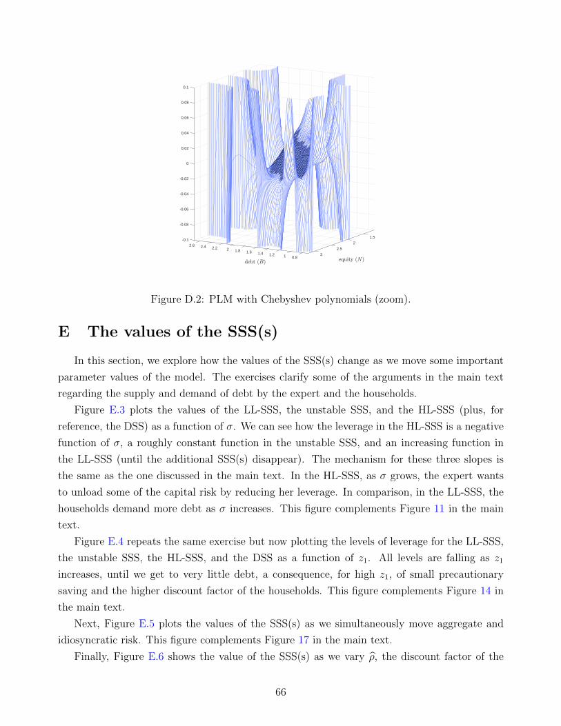
1.5-0.1

-0.08

2

-0.06

-0.04

-0.02

0

0.02

2.6

0.04

0.06

0.08

2.4

0.1

2.2 2.52 1.8 1.6 1.4 31.2 1 0.8

Figure D.2: PLM with Chebyshev polynomials (zoom).

E The values of the SSS(s)

In this section, we explore how the values of the SSS(s) change as we move some important

parameter values of the model. The exercises clarify some of the arguments in the main text

regarding the supply and demand of debt by the expert and the households.

Figure E.3 plots the values of the LL-SSS, the unstable SSS, and the HL-SSS (plus, for

reference, the DSS) as a function of σ. We can see how the leverage in the HL-SSS is a negative

function of σ, a roughly constant function in the unstable SSS, and an increasing function in

the LL-SSS (until the additional SSS(s) disappear). The mechanism for these three slopes is

the same as the one discussed in the main text. In the HL-SSS, as σ grows, the expert wants

to unload some of the capital risk by reducing her leverage. In comparison, in the LL-SSS, the

households demand more debt as σ increases. This figure complements Figure 11 in the main

text.

Figure E.4 repeats the same exercise but now plotting the levels of leverage for the LL-SSS,

the unstable SSS, the HL-SSS, and the DSS as a function of z1. All levels are falling as z1

increases, until we get to very little debt, a consequence, for high z1, of small precautionary

saving and the higher discount factor of the households. This figure complements Figure 14 in

the main text.

Next, Figure E.5 plots the values of the SSS(s) as we simultaneously move aggregate and

idiosyncratic risk. This figure complements Figure 17 in the main text.

Finally, Figure E.6 shows the value of the SSS(s) as we vary ρ, the discount factor of the

66

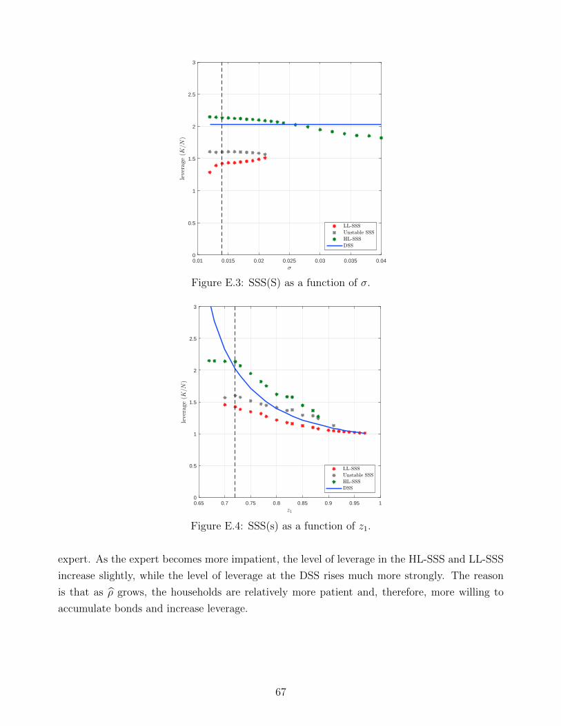
0.01 0.015 0.02 0.025 0.03 0.035 0.040

0.5

1

1.5

2

2.5

3

Figure E.3: SSS(S) as a function of σ.

0.65 0.7 0.75 0.8 0.85 0.9 0.95 10

0.5

1

1.5

2

2.5

3

Figure E.4: SSS(s) as a function of z1.

expert. As the expert becomes more impatient, the level of leverage in the HL-SSS and LL-SSS

increase slightly, while the level of leverage at the DSS rises much more strongly. The reason

is that as ρ grows, the households are relatively more patient and, therefore, more willing to

accumulate bonds and increase leverage.

67

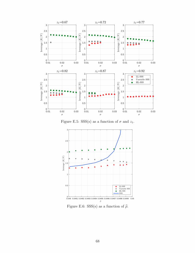
0.01 0.02 0.030

0.5

1

1.5

2

2.5

3

0.01 0.02 0.030

0.5

1

1.5

2

2.5

3

0.01 0.02 0.030

0.5

1

1.5

2

2.5

3

0.01 0.02 0.030

0.5

1

1.5

2

2.5

3

0.01 0.02 0.030

0.5

1

1.5

2

2.5

3

0.01 0.02 0.030

0.5

1

1.5

2

2.5

3

Figure E.5: SSS(s) as a function of σ and z1.

0.049 0.0491 0.0492 0.0493 0.0494 0.0495 0.0496 0.0497 0.0498 0.0499 0.050

0.5

1

1.5

2

2.5

3

Figure E.6: SSS(s) as a function of ρ.

68

F Value functions

The second row of Figure F.7 plots the value functions of the households as a function of

assets for low- and high-labor productivity at the HL-SSS and the LL-HHH. For easy reference,

in the first row of Figure F.7, we reproduce the distributions of households.

0 2 4 6 8 100

0.01

0.02

0.03

0.04

0 2 4 6 8 100

0.2

0.4

0.6

0.8

1

0 2 4 6 8 100

1

2

3

4

5

6

7

0 2 4 6 8 100

1

2

3

4

5

6

7

0 2 4 6 8 10-0.08

-0.06

-0.04

-0.02

0

0.02

0.04

0.06

0 2 4 6 8 10-0.08

-0.06

-0.04

-0.02

0

0.02

0.04

0.06

Figure F.7: Wealth distribution and value functions in the DSS and SSS.

The comparison of value functions shows that, for all levels of assets, households prefer to be

at the LL-SSS than at the HL-SSS. This fact is not a surprise since at the LL-SSS the economy

is less volatile and households have concave preferences only over consumption (not allowing,

therefore, substitution with leisure when productivity is low). However, precautionary behavior

also means that, at the HL-SSS, we will have more rich households.

Lastly, the bottom row of Figure F.7 shows how the value function changes after a two-

standard-deviations negative capital shock: poorer households are worse off (they have lower

wages), but wealthier households are better off, as their bonds pay a higher interest rate. The

effect is more acute at the HL-SSS, as the persistence of wages and the risk-free interest rate is

higher.

69