WP/14/194

Financial Frictions and Sources of Business Cycle

Marzie Taheri Sanjani

© 2014 International Monetary Fund WP/ 14/194

IMF Working Paper

European Department

Financial Frictions and Sources of Business Cycle

Prepared by Marzie Taheri Sanjani 1

Authorized for distribution by Ernesto Ramirez Rigo

October 2014

Abstract

This paper estimates a New Keynesian DSGE model with an explicit financial intermediary sector. Having measures of financial stress, such as the spread between lending and borrowing, enables the model to capture the impact of the financial crisis in a more direct and efficient way. The model fits US post-war macroeconomic data well, and shows that financial shocks play a greater role in explaining the volatility of macroeconomic variables than marginal efficiency of investment (MEI) shocks.

JEL Classification Numbers: C11, E44, E47, E52, E58

Keywords: DSGE, Bayesian Estimation, Financial Frictions, Sources of Business Cycle

Author’s E-Mail Address: mtaherisanjani@imf.org

1Author is grateful of Lucrezia Reichlin for her valuable guidance and thank Domenico Giannone, Andrew Scott, Martin Ellison, Leonardo Melosi, Albert Marcet, Ivanna Vladkova Hollar, Juan Paolo Nicolini, Kenneth R. Beauchemin, Peter Karadi, and Tomasz Wieladek for helpful comments. I acknowledge financial support from London Business School. The views expressed in this paper are mine and do not represent those of the IMF. All errors are my own.

This Working Paper should not be reported as representing the views of the IMF. The views expressed in this Working Paper are those of the author(s) and do not necessarily represent those of the IMF or IMF policy. Working Papers describe research in progress by the author(s) and are published to elicit comments and to further debate.

Contents

I. Introduction 2

II. Model 4A. Households . . . . . . . . . . . . . . . . . . . . . . . . . . . . . . . . . . . . . . . . . . 5B. Financial Intermediaries . . . . . . . . . . . . . . . . . . . . . . . . . . . . . . . . . . . 6C. Intermediate Good Producer Firm . . . . . . . . . . . . . . . . . . . . . . . . . . . . . 9D. Capital Producer Firm . . . . . . . . . . . . . . . . . . . . . . . . . . . . . . . . . . . 11

D.1. Tobin’s Q . . . . . . . . . . . . . . . . . . . . . . . . . . . . . . . . . . . . . . 13E. Retail Firms . . . . . . . . . . . . . . . . . . . . . . . . . . . . . . . . . . . . . . . . . 13F. Central Bank . . . . . . . . . . . . . . . . . . . . . . . . . . . . . . . . . . . . . . . . . 14G. Government Budget Constraint . . . . . . . . . . . . . . . . . . . . . . . . . . . . . . . 15H. Resource Constraint . . . . . . . . . . . . . . . . . . . . . . . . . . . . . . . . . . . . . 15

III.Empirical Evaluation 16A. Prior Distributions . . . . . . . . . . . . . . . . . . . . . . . . . . . . . . . . . . . . . . 16B. Posterior Estimates . . . . . . . . . . . . . . . . . . . . . . . . . . . . . . . . . . . . . 19

IV. Model Fit 20

V. Drivers of Business Cycle 22

VI.Impulse Response Functions 25

VII.Conclusion 28

A Appendix - Data 31

List of Tables

1 Prior Distributions and Posterior Parameter Estimates in the Model . . . . . . . 182 Marginal Data Density Test . . . . . . . . . . . . . . . . . . . . . . . . . . . . . . 213 Theoretical Moments (standard deviation and 3 lags autocorrelation) . . . . . . . . . 224 Variance Decompositions (%) . . . . . . . . . . . . . . . . . . . . . . . . . . . . . 23

List of Figures

1 Growth and TED spread (left axis) and credit spread (right axis) . . . . . . . . . . . 32 Economy with financial intermediary . . . . . . . . . . . . . . . . . . . . . . . . . . . 53 Brooks and Gelman’s convergence diagnostics . . . . . . . . . . . . . . . . . . . . . . 194 Smoothed financial shocks and default risk spread . . . . . . . . . . . . . . . . . . . . 195 Normalized impulse response functions to MEI and capital quality shocks . . . . . . . 256 Impulse responses to technology (blue) and monetary policy (red) shocks . . . . . . . 267 Impulse responses to capital quality shock . . . . . . . . . . . . . . . . . . . . . . . . . 27

2

3

I. Introduction

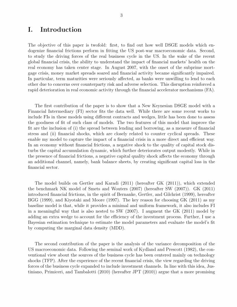
The objective of this paper is twofold: first, to find out how well DSGE models which en-dogenize financial frictions perform in fitting the US post-war macroeconomic data. Second,to study the driving forces of the real business cycle in the US. In the wake of the recentglobal financial crisis, the ability to understand the impact of financial markets’ health on thereal economy has taken center stage. In August 2007, with the onset of the subprime mort-gage crisis, money market spreads soared and financial activity became significantly impaired.In particular, term maturities were seriously affected, as banks were unwilling to lend to eachother due to concerns over counterparty risk and adverse selection. This disruption reinforced arapid deterioration in real economic activity through the financial accelerator mechanisms (FA).

The first contribution of the paper is to show that a New Keynesian DSGE model with aFinancial Intermediary (FI) sector fits the data well. While there are some recent works toinclude FIs in these models using different contracts and wedges, little has been done to assessthe goodness of fit of such class of models. The two features of this model that improve thefit are the inclusion of (i) the spread between lending and borrowing, as a measure of financialstress and (ii) financial shocks, which are closely related to counter cyclical spreads. Theseenable my model to capture the impact of a financial crisis in a more direct and efficient way.In an economy without financial frictions, a negative shock to the quality of capital stock dis-turbs the capital accumulation dynamic, which further deteriorates output modestly. While inthe presence of financial frictions, a negative capital quality shock affects the economy throughan additional channel, namely, bank balance sheets, by creating significant capital loss in thefinancial sector.

The model builds on Gertler and Karadi (2011) (hereafter GK (2011)), which extendedthe benchmark NK model of Smets and Wouters (2007) (hereafter SW (2007)). GK (2011)introduced financial frictions, in the spirit of Bernanke, Gertler, and Gilchrist (1999), hereafterBGG (1999), and Kiyotaki and Moore (1997). The key reason for choosing GK (2011) as mybaseline model is that, while it provides a minimal and uniform framework, it also includes FIin a meaningful way that is also nested to SW (2007). I augment the GK (2011) model byadding an extra wedge to account for the efficiency of the investment process. Further, I use aBayesian estimation technique to estimate the model parameters and evaluate the model’s fitby computing the marginal data density (MDD).

The second contribution of the paper is the analysis of the variance decomposition of theUS macroeconomic data. Following the seminal work of Kydland and Prescott (1982), the con-ventional view about the sources of the business cycle has been centered mainly on technologyshocks (TFP). After the experience of the recent financial crisis, the view regarding the drivingforces of the business cycle expanded to include investment channels. In line with this idea, Jus-tiniano, Primiceri, and Tambalotti (2010) (hereafter JPT (2010)) argue that a more promising

4

theory is one that largely attributes fluctuations to investment shocks and, more specifically,to marginal efficiency of investment (MEI) shocks. MEI shocks are exogenous disturbanceswhich affect the efficiency of the process that transforms current investment goods to futureproductive capital.

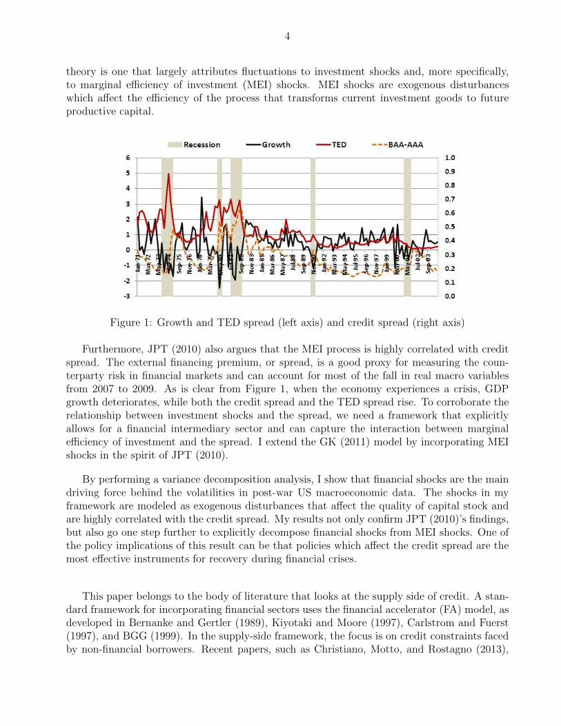
Figure 1: Growth and TED spread (left axis) and credit spread (right axis)

Furthermore, JPT (2010) also argues that the MEI process is highly correlated with creditspread. The external financing premium, or spread, is a good proxy for measuring the coun-terparty risk in financial markets and can account for most of the fall in real macro variablesfrom 2007 to 2009. As is clear from Figure 1, when the economy experiences a crisis, GDPgrowth deteriorates, while both the credit spread and the TED spread rise. To corroborate therelationship between investment shocks and the spread, we need a framework that explicitlyallows for a financial intermediary sector and can capture the interaction between marginalefficiency of investment and the spread. I extend the GK (2011) model by incorporating MEIshocks in the spirit of JPT (2010).

By performing a variance decomposition analysis, I show that financial shocks are the maindriving force behind the volatilities in post-war US macroeconomic data. The shocks in myframework are modeled as exogenous disturbances that affect the quality of capital stock andare highly correlated with the credit spread. My results not only confirm JPT (2010)’s findings,but also go one step further to explicitly decompose financial shocks from MEI shocks. One ofthe policy implications of this result can be that policies which affect the credit spread are themost effective instruments for recovery during financial crises.

This paper belongs to the body of literature that looks at the supply side of credit. A stan-dard framework for incorporating financial sectors uses the financial accelerator (FA) model, asdeveloped in Bernanke and Gertler (1989), Kiyotaki and Moore (1997), Carlstrom and Fuerst(1997), and BGG (1999). In the supply-side framework, the focus is on credit constraints facedby non-financial borrowers. Recent papers, such as Christiano, Motto, and Rostagno (2013),

5

Mandelman (2010), Nolan and Thoenissen (2009), Ajello (2010), and Hirakata, Sudo, and Ueda(2011), draw attention to the importance of financial shocks in explaining business cycle fluc-tuations. Liu, Waggoner, and Zha (2011) emphasizes the key role of shocks on the capitaldepreciation rate and further argue that these shocks resemble financial shocks.

The paper proceeds as follows. The model is described in section 2. Section 3 details theempirical evaluation of the model. The model fit is presented in section 4. Section 5 shows theresult of variance decompositions. The policy implications and impulse responses are discussedin section 6 and section 7 concludes the paper. Data description is included in the appendix.

II. Model

This section describes my model of business cycles for the US economy. It is a standard DSGEmodel which is based upon GK (2011). The core macro model is kept simple in order to high-light the role of intermediation. Among the models with financial intermediaries, GK (2011) is agood framework for empirical studies for two reasons. Firstly, because the model is nested withCEE (2005) and SW (2007). In an ideal world without financial frictions there is no role forthe banking sector, and the model is isomorphic to those standard NK models. Furthermore,both of those models fit the data well and are capable of explaining the sources of businesscycle that are proposed in the literature. The second reason for picking the Gertler and Karadiframework is that inclusion of financial intermediaries without making the model too complexhas a substantial effect on model dynamics and policy implications.

Figure 2: Economy with financial intermediary

The model has seven sectors: Households (HH), Financial intermediaries (FI), Central bank(CB), Government (Gov), Non-financial goods producer firm (GPF), Capital producer firms(CPF), Monopolistically competitive retail firms (RF). The latter are in the model only to

6

introduce nominal price rigidities. One important feature of the model is the inclusion of ahomogenous financial intermediary sector that contains a moral hazard type of financial ac-celerator mechanism. Financial intermediaries in this model are simplified and they form ahomogenous sector that is meant to capture the entire banking sector, essentially investmentbanks as well as commercial banks. They transfer funds between households and non-financialfirms. The source of financial frictions in the model is the moral hazard incentive constraintthat limits the ability of financial intermediaries to obtain funds from households. The seconddistinguishing feature of the model is allowing for an investment shock that determines theefficiency of newly produced investment goods, the so-called marginal efficiency of investmentshock, as in Greenwood, Hercowitz, and Huffman (1988).

A. Households

The economy is populated with a continuum of identical households. Households’ utility isa function of consumption with habit formation and labor. Each household saves by lendingfunds to competitive financial intermediaries or, potentially, to the government. Within eachhousehold there are two types of agents. At any point in time 1− f fraction of households are”workers” and the remaining f fraction of them are ”bankers”; moreover, they can also switchbetween occupations with a historically independent probability. This set up allows for hav-ing a similar coefficient of intertemporal time preference between bankers and workers, whichresults in perfect consumption smoothing. Workers are monopolistic competitors in the labormarket, where they get a wage for supplying their labor. They, further, return their wages tothe households, while bankers manage a financial intermediary and also transfer earnings backto households. With i.i.d probability 1 − θ, a banker exits next period, so at each period, atotal measure of (1− θ)f bankers randomly become workers and the same fraction of workersshould transit to being bankers to keep the measure of each type constant. Upon exit, bankerstransfer retained earnings to the households and new bankers receive some ”startup” funds fromthe family (household). In order to keep the measure in each occupation constant, the modelallows the same fraction of agents to transit from being workers to being bankers. There is afinite horizon for bankers to prevent the limiting case of funding the investment opportunitiesentirely from bankers’ capital.

In my representative agent setup, households consume Ct, buy one period real bond Bt

which pays the gross real rate Rt from banks or the government, supply labor Lt in exchangefor wage Wt, pay lump-sum tax Tt to the government, and receive the net transfer Πt whichis the funds transferred from existing bakers minus the funds transferred to new bankers. Thehousehold utility maximization problem is the following:

maxCt,Lt Et

∞∑i=0

βibt+i[log(Ct+i − hCt+i−1)− χ

1− φL1+φt+i ] (1)

s.t. Ct +Bt+1 = WtLt +RtBt + Πt − Tt, (2)

7

where χ is the coefficient of leisure, h is the habit persistence parameter, φ is the inverseFrisch parameter, bt is intertemporal preference shock, which affects both the marginal utilityof consumption and the marginal disutility of labor. It follows an AR(1) process, as below,with the ρb persistence and σb variance:

log bt = ρb log bt−1 + σbεb,t, (3)

where εb,t ∼ i.i.d.N(0, 1). Since technological progress is non-stationary, the log utilityensures the existence of a balanced growth path. Note that I do not assume an exogenousprocess for the coefficient of leisure, χ. β is the time discount factor. In another exercise,which is not reported here, I found that variance decomposition analysis shows that this shockis not an important shock in explaining the volatility of macroeconomic data. The first ordercondition of the household optimization problem implies:

ρtWt = χtLφt (4)

βEtΛt,t+1Rt+1 = 1, (5)

where marginal utility of consumption is ρt = bt(Ct − hCt−1)−1 − βhEtbt+1(Ct+1 − hCt)−1 andΛt,t+1 ≡ ρt+1

ρt. Equation 5 is known as the Euler equation.

B. Financial Intermediaries

Bankers transfer funds from savers (households) to investors (good producer firms). Financialintermediaries are indexed by j. At the beginning of the period, each bank raises deposits Bjt

from households in the retail financial market at the risk-free rate Rt+1, which is paid at periodt + 1. Then they purchase financial claims St from goods producer firms with relative priceQt. Banker’s equity capital, or net worth, at the end of period t is Nt, which is the differencebetween the assets and the liabilities. Hence, the balance sheet of the intermediary j is givenby:

Assets LiabilitiesQtSt Bt

Nt

Nj,t = QtSj,t −Bj,t. (6)

At period t + 1 claims on non-financial firms pay out the stochastic return Rk,t+1. Notethat, as I will show later, both Rk,t+1 and Rt+1 are endogenous variables. Bankers’ net worthdynamic evolves as net earnings on assets minus the interest payments on liabilities:

8

Nj,t+1 = Rk,t+1QtSj,t −Rt+1Bj,t (7)

Nj,t+1 = Rt+1Nj,t + (Rk,t+1 −Rt+1)QtSj,t, (8)

where (Rk,t+1 −Rt+1) represent the interest rate spread or the external financing premium.Net worth grows at rate R and any expansion comes from excess return on financial assets(Rk,t+1−Rt+1)QtSj,t. It follows that the spread is related to financial frictions in the model. Thenecessary condition for the bankers to stay in business is that the discounted expected returnon non-financial claims should be greater than or equal to the discounted cost of borrowingfrom households; this implies that the discounted spread should be nonnegative:

βiΛt,t+1+i(Rk,t+1+i −Rt+1+i) ≥ 0, ∀i ≥ 0,

where at time t, βiΛt,t+1+i is the stochastic discount factor for i period ahead return. Thebanker accumulates net worth before exit and her value function at time t, Vj,t, is to maximizeher net present value of her expected equity capital. The expected terminal wealth follows by:

max{Vj,t ≡ (1− θ)Et{∞∑i=0

θiβiΛt,t+1+i(Nj,t+1+i)} (9)

≡ (1− θ)Et{∑∞i=0 θiβiΛt,t+1+i(Rt+1+iNj,t+i + (Rk,t+1+i −Rt+1+i)Qt+iSj,t+i)}.

I can rewrite the value of the bank at the end of period t− 1, as a Bellman equation:

Vt−1(Sj,t−1, Bj,t−1) = Et−1{Λt−1,tNj,t}+ maxSj,t

Vt(Sj,t, Bj,t). (10)

To solve the decision problem, one can show that the value function is linear:

Vj,t = νtQtSj,t + ηtNj,t, (11)

where νt and ηt are time varying parameters. Note that νt is the marginal value of assetsat the end of period t and ηt is the marginal cost of deposits, as follows:

9

νt = Et{(1− θ)(Rkt+1 −Rt+1) + βΛt,t+1θxt,t+1νt+1} (12)

ηt = Et{(1− θ)Rt+1 + βΛt,t+1θzt,t+1ηt+1} (13)

xt,t+1 ≡Qt+iSj,t+iQtSj,t

(14)

zt,t+1 ≡Nj,t+i

Nj,t

. (15)

In the economy without financial frictions, the banker wants to expand her assets by borrow-ing from households infinitely. In order to limit bankers’ borrowing ability, financial frictionsin the form of the moral hazard problem is introduced. In each period the banker can chooseto divert a fraction λ of her total assets QtSj,t back to her family. If a bank diverts assets forits personal benefit, it defaults on its debt. The creditors can reclaim the remaining fraction(1− λ) of funds. Since the creditors are aware of this moral hazard incentive, they will restrictthe amount they lend to the bank. Let Vt(Sj,t, Bj,t) be the maximized value of Vt, given thebalance sheet configuration (Sj,t, Bj,t) at the end of period t. Next, the moral hazard incentivecondition ensure that the bank does not divert funds:

Vt(Sj,t, Bj,t) ≥ λQtSj,t. (16)

The value of staying in business should be greater than diverting some fund and defaultingon the rest. When the constraint binds, assets will be a levered ratio (φt) of net worth:

QtSj,t =ηt

λ− νtNj,t (17)

QtSj,t = φtNjt, (18)

where φt = ηtλ−νt is the leverage ratio of financial intermediary.

Net worth Dynamic:The net worth of existing bankers evolves as:

Nt = θ[(Rk,t −Rt)φt +Rt]Nt−1,

Note that the net worth of the existing banker does not include any wealth shock, as, in anotherexercise which is not reported here, I found that variance decomposition analysis shows thatthis shock plays virtually no role in explaining the business cycle. At each period, a fraction of(1−θ) bankers become workers and transfer their accumulated net worth QtSt to households. A

10

fraction ω1−θ of this transfer will be given to new bankers who enter at period t+ 1, (0 < ω < 1)

as their start-up net worth, Nnt:

Nnt =ω

1− θ(1− θ)QtSt−1 = ωQtSt−1. (19)

Aggregate net worth at any period t is the sum of the net worth of existing bankers (Net) andnew bankers (Nnt):

Nt = Net +Nnt (20)

Nt = θ[(Rk,t −Rt)φt +Rt]Nt−1 + ωQtSt−1. (21)

Financial intermediaries also issue loans to non-financial goods producer sectors by pur-chasing their financial claims at unit price of capital. The loans are further used in productionof intermediary goods. In the following section I describe the role of the intermediate goodsproducer firm in detail.

C. Intermediate Good Producer Firm

Non-financial goods producer firms are competitive. They have Cobb-Douglas constant returns-to-scale technology that uses labor and capital to produce intermediate good Yt. At the end ofany period t, they issue stocks (St) equal to the number of units of capital they need. They,further, sell the stocks at the price of unit of capital Qt, in order to raise the required capital,which is going to be used in the next period production. Hence, by the arbitrage condition, thefollowing equality should hold:

QtKt+1 = QtSt.

I will show in the next section that the shadow price Qt is drawn endogenously from profitmaximization of the capital producer firm. Production takes place at time t. Capital is notmobile, but labor is perfectly mobile across firms and this allows expressing aggregate outputYt as a function of effective aggregate capital Kt and aggregate labor hours Lt as below. Notethat Ut is the time-varying utilization rate of the capital and ξtKt is the effective quantity ofcapital:

Yt = At(UtξtKt)αL1−α

t (22)

logAt = ρA logAt−1 + σAεA,t (23)

log ξt = (1− ρξ) log ξss + ρ log ξt−1 + σξεξ,t. (24)

11

α is the share of capital in the production function. AR(1)At is aggregate productivitywhich follows a Markov process, with εA,t ∼ i.i.d.N(0, 1). The model is stationary so At doesnot contain stochastic growth. The shock ξt is meant to capture the exogenous disturbances tothe quality of productive capital; it also resembles distortions to the capital depreciation rate.The later captures the microeconomic frictions that effects intertemporal capital accumulationchoice. ξt follows AR(1) stochastic exogenous process with εξ,t ∼ i.i.d.N(0, 1). Following BGG(1999), retailers purchase the intermediate good from non-financial good producer firms at thewholesale price Pmt and transform it into a composite final good, whose price index is Pt. Withthis notation, Pt/Pmt denotes the markup of final over intermediate goods. Production takesplace at t+ 1 and intermediate goods are sold to retail firms at the price Pm,t+1. Firm’s profitis given by:

Υt+1 = EtβΛt,t+1[Pm,t+1Yt+1 + (Qt+1 − δ(Ut+1))ξt+1Kt+1 −Rk,t+1QtKt+1 −Wt+1Lt+1]. (25)

The model assumes that the replacement price of depreciated capital is unity and, giventhat Qt is the price of capital stock, (Qt+1 − δ(Ut+1))ξt+1Kt+1 gives the value of the leftovercapital. The depreciation rate varies with utilization and is assumed to follow the functionalform:

δ(Ut) = δss +b

1 + ζU1+ζt , (26)

where δss is determined by the steady state and ζ is the elasticity of utility cost. Optimalchoice of wage Wt, utilization rate Ut, and rental rate Rkt are given by the first order conditionsof firm’s state-by-state profit maximization problem, as below:

∂Υt

∂Lt= 0 : Pm,t(1− α)

YtLt

= Wt (27)

∂Υt

∂Ut= 0 : Pm,tα

YtUt

= δ′(Ut)ξtKt (28)

∂Υt+1

∂Kt+1

= 0 : Rkt+1 =Pmt+1α

Yt+1

Kt+1+ (Qt+1 − δ(Ut+1))ξt+1

Qt

. (29)

The last equation relates the return on capital, Rkt, to the financial shock, ξt. This implieswhen there is a negative exogenous disturbances to the quality of productive capital, rental costincreases and this further deteriorates the net worth of bankers. This is the key to understanding

12

the dynamic of spread; later, in section 6, I show how the correlation between spread and capitalquality shock plays a major role in explaining volatility in US macroeconomic variables. In thenext section I will describe the role of the capital producer firm and the dynamic of capitalaccumulation. Presence of a representative capital producer sector allows for a meaningful wayof decomposing out financial shock from marginal efficiency of investment shock, through thedynamic of capital. I will also show how the shadow price is related to the MEI shock.

D. Capital Producer Firm

Capital producer firms are competitive. At the end of each period t, they buy the depreciatedcapital from intermediate good producer firms at price Q̄t. They repair depreciated capital,and sell both the refurbished and the new capital at price Qt. Let It denote the investmentexpenditures; then capital accumulation dynamic is given by:

Kt+1 = (1− δ(Ut))ξtKt + γtΦ(ItKt

)Kt. (30)

The second term shows the adjustment cost of capital and γt represents the MEI shockwhich follows an AR(1) stochastic process. MEI shock represents exogenous disturbance tothe process by which investment goods are transformed into installed capital to be used inproduction. JPT (2010) argues that the MEI shocks represent disturbances to the process bywhich investment goods are turned into capital ready for production. The classical Keynesiantheory relates MEI to the responsiveness of investment to changes in the interest rate spread. Afall in interest rate spread should decrease the cost of investment relative to the potential yieldand, as a result planned capital investment projects on the margin may become worthwhile.Therefore, the efficiency of the investment process is closely linked to the health of the financialsystem. In the real world, because of the presence of friction in financial market, the investmentprocess is not entirely efficient and it encounters randomness, uncertainty, and waste of physicalresources while adjusting the investment rate. Introducing the MEI shock is a way to capturesuch inefficiencies:

log γt = ρi log γt−1 + σγεγ,t, (31)

where εγ,t ∼ i.i.d.N(0, 1). JPT (2010) shows that the business cycles are driven primarilyby MEI shocks, as opposed to the shocks that affect the transformation of consumption intoinvestment goods (IST shocks). In the next section, I will present evidence that in the presenceof the financial frictions, MEI shocks play only a minor role in explaining the business cyclefluctuations; this is while the capital quality shocks can account for most of the cyclical varia-tions in the aggregate macroeconomic variables.

13

Following BGG (1999), I assume that there are increasing marginal adjustment costs in theproduction of capital, which I capture by assuming that investment expenditures of It yield agross output of new capital goods Φ( I

Kt)Kt, where Φ is an increasing and concave function where

Φ(0) = 0. I include adjustment costs to permit a variable price of capital.1 In equilibrium,given the adjustment cost function, the price of a unit of capital in terms of the numerairegood, Qt, is given by:

Qt = (Φ′(ItKt

))−1. (32)

I assume the following conventional form for Φ(.):

Φ(ItKt

) = [1− S(ItIt−1

)]ItKt

, (33)

where the function S captures the presence of adjustment costs in investment. As in CEE(2005), firms face quadratic adjustment costs on construction of new capital. In particular, thecosts are quadratic in deviations of the growth in investment from a value of unity:

S(ItIt−1

) =ηi2

(ItIt−1

− 1)2. (34)

Note that S ′(.) > 0, S”(.) > 0, S(1) = S ′(1) = 0. ηi is the inverse elasticity of net investmentto the price of capital. The law of capital motion is then given by:

Kt+1 = ξt(1− δ(Ut))Kt + γt[1− S(ItIt−1

)]It. (35)

D.1. Tobin’s Q

Capital producer firm’s profit per unit of capital at period t is given by:

Ψt = QtγtΦ(ItKt

)− ItKt

− (Q̄t −Qt). (36)

Firm maximizes its total discounted profit:

maxIt{Et

∞∑i=t

βiΛt,i{QiγiΦ(IiKi

)Ki − Ii − (Q̄i −Qi)Ki}}.

1As in Kiyotaki and Moore (1997), therefore the idea is to have asset price variability which contributes tovolatility in entrepreneurial net worth.

14

I rewrite the profit equation by substituting adjustment cost from above, as follows:

maxIt{Et

∞∑i=t

βiΛt,i{Qiγi[(1− S(ItIt−1

))It]− Ii − (Q̄i −Qi)Ki}}. (37)

The profit maximization problem of capital producer firms implies that the shadow price ofcapital is given by:

Qt = arg maxIt{Et

∞∑i=t

βiΛt,i{Qiγi[(1− S(ItIt−1

))It]−

Ii − (Q̄i −Qi)Ki}} (38)

Qtγt[1− S(ItIt−1

)− S ′( ItIt−1

)(ItIt−1

)] +

βEt{Qt+1Λt,t+1γt+1S′(It+1

It)(It+1

It)2} = 1. (39)

E. Retail Firms

The retail sector in this model is a standard RBC sector that generates nominal rigidity, follow-ing CEE (2005). At every point in time t, perfectly competitive firms purchase the intermediategoods Ymt at price Pmt and re-package them and set the price on a staggered basis, as in Calvo(1983). The derivations of formulas in this section are standard, therefore without going intothe details of equations, I just mention the essence of the sticky price mechanism. The wholesaleretail output is:

Yt = YmtDt, (40)

where Dt is price dispersion and is given by:

Dt = $Dt−1π−γP εpt−1 π

εpt + (1−$)(

1−$π−γP (1−$)t−1 π$−1

t

1−$)−

εp1−$ . (41)

Note that the $ is the Calvo probability, which is the probability of keeping the price fixed.γP is the measure of price indexation and εP is the elasticity of substitution. The recursiveformulation of the optimal price choice is given by:

15

Yt = YtPmt + Et[β$Λt,t+1π−(γP εP )t

π−εPt+1

Ft+1] (42)

Zt = Yt + Et[β$Λt,t+1πγP (1−εP )t

π(1−εP )t+1

Zt+1] (43)

π∗t =1

τX

εPεP − 1

FtZtπt. (44)

Therefore, it will follows that the inflation dynamic has the bellow standard form:

π1−εPt = $π

γP (1−εP )t−1 + (1−$)π

∗(1−εP )t . (45)

F. Central Bank

The central bank has a conventional monetary policy instrument by which it sets the nominalinterest rate following a feedback rule of the form:

(iti

) = (it−1

i)ρr(

(πtπ∗

)κπ(YtY ∗t

)κy)(1−ρr)

eσiεi,t , (46)

where ρr sets the degree of interest rate smoothing and i is the steady state of the grossnominal interest rate. The interest rate responds to the deviations of inflation from its steadystate and the output gap; κπ and κy are the corresponding control parameters. Finally, themonetary policy rule is also disturbed by a monetary policy shock εi,t ∼ i.i.d.N(0, 1). Thenominal and risk-free interest rates satisfy the Fisher equation:

it = Rt+1Etπt+1, (47)

where Rt is real interest rate (RIR).

16

G. Government Budget Constraint

Government finances its exogenous expenditure Gt by collecting the lump-sum tax Tt (or subsi-dies) that also appear in households’ budget constraint. Consequently, the government’s budgetconstraint is given by:

Gt = Tt, (48)

where government spending is subject to a stochastic shock and follows as:

Gt = (1− 1/gt)Yt (49)

log gt = (1− ρg) log gss + ρg log gt−1 + σgεg,t (50)

εg,t ∼ i.i.d.N(0, 1), (51)

where gss is the steady state value of government spending.

H. Resource Constraint

Output is divided between consumption, investment, adjustment cost of investment, and gov-ernment consumption Gt; hence, the aggregate resource constraint is given by:

Yt = Ct + It + S(ItIt−1

)It +Gt. (52)

Equations (1) to (52) determine twelve endogenous variables. The stochastic behavior ofthe system of linear rational expectations equations is driven by six exogenous disturbances:intertemporal preference shifter (bt), total factor productivity (At), marginal efficiency of in-vestment (γt ), capital quality (ξt ), government spending (gt), and monetary policy (εi) shocks.In the next section I will explain the empirical evaluations of the model.

III. Empirical Evaluation

The model presented in the previous section is estimated with Bayesian estimation techniques.I use four key macroeconomic quarterly US time series as observable variables: the log difference

17

of real GDP per capita, the log difference of real investment per capita, the log difference of theGDP deflator, and the federal funds rate. The model is expressed in log deviation from steadystate for simulation purposes. Real per-capita GDP is obtained by dividing the real GDP bythe civilian non-institutional population (16 years and over). Real per-capita investment is thenominal private investment, divided by the civilian non-institutional population and the GDPdeflator. The inflation rate is the log difference of the GDP deflator. All series are seasonallyadjusted. The interest rate is the Federal Funds Rate. GDP and investment are expressed in100 times log. The inflation rate and interest rate are expressed on a quarterly basis. GDP,investment, and the deflator are obtained from the US Department of Commerce, Bureau ofEconomic Analysis. Civilian non-institutional population (16 years and over) is obtained fromUS Department of Labor, Bureau of Labor Statistics. Federal Funds Rate is obtained fromFederal Reserve Economic Data - FRED - St. Louis Fed. The corresponding measurementequation is:

yd =

∆log(GDPt)∆log(INVt)

∆log(Pt)FedFundt

=

Y (t)− Y (t− 1)I(t)− I(t− 1)

π(t)i(t)

,

where ∆log stands for the log difference. I use quarterly data from 1962Q1 to 2004Q4 andestimate the posterior modes by maximizing the log posterior function, which combines theprior information on the parameters with the likelihood of the data. In what follows I explainprior assumptions and details of my Bayesian estimation steps.

A. Prior Distributions

The standard errors of the innovations are assumed to follow an inverse-gamma distributionwith a mean of 0.10 and a standard deviation of 2.0, which corresponds to a rather loose prior.The covariance matrix of the innovations is diagonal. The persistence of AR(1) processes isbeta distributed with a mean of 0.5 and a standard deviation of 0.2. Priors for structuralparameters are set following the standard measures in the literature (SW (2007), JPT (2010)).Table 1 summarizes the prior and posterior distributions of the parameters in the model. Inv.Gamma represents Inverse Gamma distribution.

Six parameters are fixed in the estimation procedure. The steady state of the depreciationrate is fixed at 0.02 and the exogenous spending-GDP ratio is set at 0.2. Both of these param-eters would be difficult to estimate unless the investment and exogenous spending ratios wouldbe directly used in the measurement equation. Discount factor (β) is set to 0.99, inverse Frischelasticity of labor is set to 0.275, banker survival rate is set to 0.971 following GK (2011), andproportional transfer to entering bankers (ω) is set to 2× 105.

18

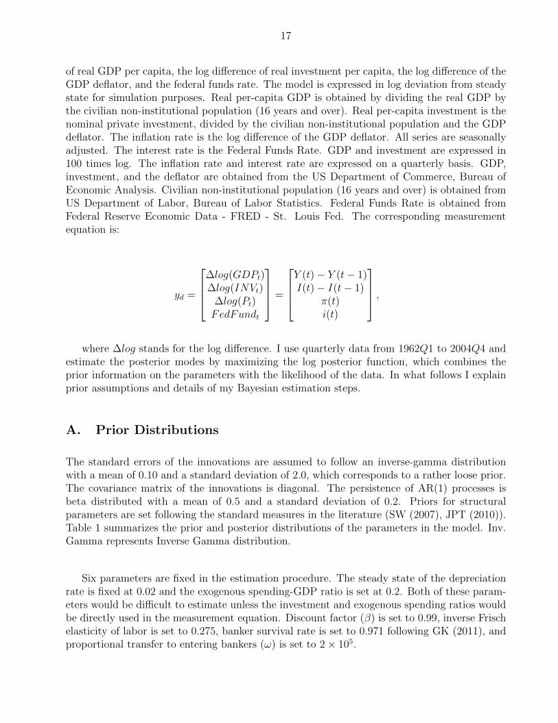
Bayesian Estimation. The Metropolis-Hastings algorithm is used to obtain a completepicture of the posterior distribution and to evaluate the marginal likelihood of the model. Isimulate the model for 20,000 Metropolis-Hastings iterations. The model is estimated overthe full sample period. Figure 3 shows the multivariate convergence statistic of the MCMCsimulation. The red and blue lines represent specific within- and between-chain measures. Theinterval statistic, presented in the top panel, is constructed around the parameter mean. TheM2 statistic, presented in the middle panel, is a measure of the variance. M3, depicted in thebottom panel, AR(1) is based on third moments. Simulation converges when the red and bluelines get close and settle down. As is clear in the graph, convergence only occurs after 10,000draws.2

0.2 0.4 0.6 0.8 1 1.2 1.4 1.6 1.8 2

x 104

7

8

9

10

11

Interval

0.2 0.4 0.6 0.8 1 1.2 1.4 1.6 1.8 2

x 104

8

10

12

14

16

m2

0.2 0.4 0.6 0.8 1 1.2 1.4 1.6 1.8 2

x 104

40

60

80

100

m3

Figure 3: Brooks and Gelman’s convergence diagnostics

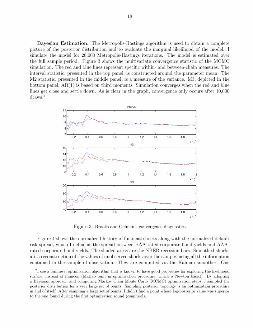
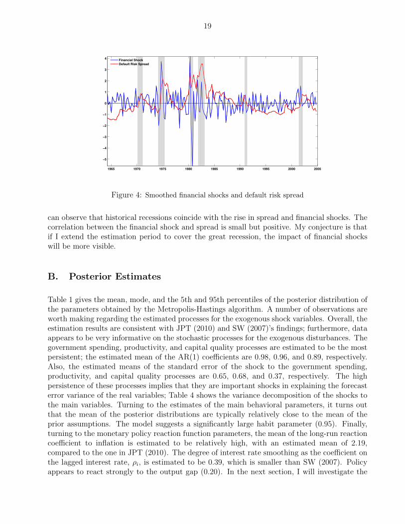
Figure 4 shows the normalized history of financial shocks along with the normalized defaultrisk spread, which I define as the spread between BAA-rated corporate bond yields and AAA-rated corporate bond yields. The shaded areas are the NBER recession bars. Smoothed shocksare a reconstruction of the values of unobserved shocks over the sample, using all the informationcontained in the sample of observation. They are computed via the Kalman smoother. One

2I use a csminwel optimization algorithm that is known to have good properties for exploring the likelihoodsurface, instead of fmincon (Matlab built in optimization procedure, which is Newton based). By adoptinga Bayesian approach and computing Markov chain Monte Carlo (MCMC) optimization steps, I sampled theposterior distribution for a very large set of points. Sampling posterior topology is an optimization procedurein and of itself. After sampling a large set of points, I didn’t find a point whose log-posterior value was superiorto the one found during the first optimization round (csminwel).

19

1965 1970 1975 1980 1985 1990 1995 2000 2005

−5

−4

−3

−2

−1

0

1

2

3

4

Financial Shock

Default Risk Spread

Figure 4: Smoothed financial shocks and default risk spread

can observe that historical recessions coincide with the rise in spread and financial shocks. Thecorrelation between the financial shock and spread is small but positive. My conjecture is thatif I extend the estimation period to cover the great recession, the impact of financial shockswill be more visible.

B. Posterior Estimates

Table 1 gives the mean, mode, and the 5th and 95th percentiles of the posterior distribution ofthe parameters obtained by the Metropolis-Hastings algorithm. A number of observations areworth making regarding the estimated processes for the exogenous shock variables. Overall, theestimation results are consistent with JPT (2010) and SW (2007)’s findings; furthermore, dataappears to be very informative on the stochastic processes for the exogenous disturbances. Thegovernment spending, productivity, and capital quality processes are estimated to be the mostpersistent; the estimated mean of the AR(1) coefficients are 0.98, 0.96, and 0.89, respectively.Also, the estimated means of the standard error of the shock to the government spending,productivity, and capital quality processes are 0.65, 0.68, and 0.37, respectively. The highpersistence of these processes implies that they are important shocks in explaining the forecasterror variance of the real variables; Table 4 shows the variance decomposition of the shocks tothe main variables. Turning to the estimates of the main behavioral parameters, it turns outthat the mean of the posterior distributions are typically relatively close to the mean of theprior assumptions. The model suggests a significantly large habit parameter (0.95). Finally,turning to the monetary policy reaction function parameters, the mean of the long-run reactioncoefficient to inflation is estimated to be relatively high, with an estimated mean of 2.19,compared to the one in JPT (2010). The degree of interest rate smoothing as the coefficient onthe lagged interest rate, ρi, is estimated to be 0.39, which is smaller than SW (2007). Policyappears to react strongly to the output gap (0.20). In the next section, I will investigate the

20

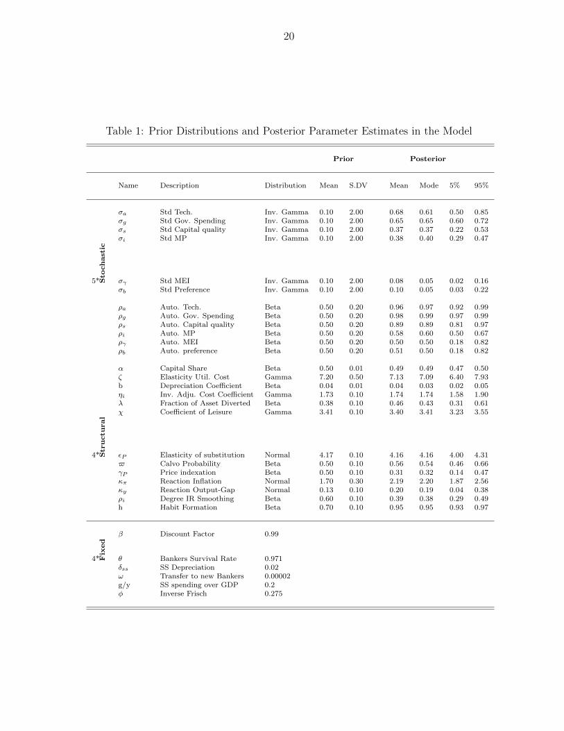
Table 1: Prior Distributions and Posterior Parameter Estimates in the Model

Prior Posterior

Name Description Distribution Mean S.DV Mean Mode 5% 95%

σa Std Tech. Inv. Gamma 0.10 2.00 0.68 0.61 0.50 0.85σg Std Gov. Spending Inv. Gamma 0.10 2.00 0.65 0.65 0.60 0.72σs Std Capital quality Inv. Gamma 0.10 2.00 0.37 0.37 0.22 0.53σi Std MP Inv. Gamma 0.10 2.00 0.38 0.40 0.29 0.47

5* Sto

chastic

σγ Std MEI Inv. Gamma 0.10 2.00 0.08 0.05 0.02 0.16σb Std Preference Inv. Gamma 0.10 2.00 0.10 0.05 0.03 0.22

ρa Auto. Tech. Beta 0.50 0.20 0.96 0.97 0.92 0.99ρg Auto. Gov. Spending Beta 0.50 0.20 0.98 0.99 0.97 0.99ρs Auto. Capital quality Beta 0.50 0.20 0.89 0.89 0.81 0.97ρi Auto. MP Beta 0.50 0.20 0.58 0.60 0.50 0.67ργ Auto. MEI Beta 0.50 0.20 0.50 0.50 0.18 0.82ρb Auto. preference Beta 0.50 0.20 0.51 0.50 0.18 0.82

α Capital Share Beta 0.50 0.01 0.49 0.49 0.47 0.50ζ Elasticity Util. Cost Gamma 7.20 0.50 7.13 7.09 6.40 7.93b Depreciation Coefficient Beta 0.04 0.01 0.04 0.03 0.02 0.05ηi Inv. Adju. Cost Coefficient Gamma 1.73 0.10 1.74 1.74 1.58 1.90λ Fraction of Asset Diverted Beta 0.38 0.10 0.46 0.43 0.31 0.61χ Coefficient of Leisure Gamma 3.41 0.10 3.40 3.41 3.23 3.55

4* Structu

ral

εP Elasticity of substitution Normal 4.17 0.10 4.16 4.16 4.00 4.31$ Calvo Probability Beta 0.50 0.10 0.56 0.54 0.46 0.66γP Price indexation Beta 0.50 0.10 0.31 0.32 0.14 0.47κπ Reaction Inflation Normal 1.70 0.30 2.19 2.20 1.87 2.56κy Reaction Output-Gap Normal 0.13 0.10 0.20 0.19 0.04 0.38ρi Degree IR Smoothing Beta 0.60 0.10 0.39 0.38 0.29 0.49h Habit Formation Beta 0.70 0.10 0.95 0.95 0.93 0.97

β Discount Factor 0.99

4* Fixed

θ Bankers Survival Rate 0.971δss SS Depreciation 0.02ω Transfer to new Bankers 0.00002g/y SS spending over GDP 0.2φ Inverse Frisch 0.275

21

fit of the model using the Bayesian model comparison method.

IV. Model Fit

How well does the model fit the data, given my posterior estimates? In this section, I try toanswer this question. Bayesian econometricians use marginal data density (MDD) to assess howwell the model fits data. I address the above question by first comparing the Laplace approx-imation of the log data density of my estimation to the one by SW (2007). This comparisoncan be insightful, as these two models are roughly nested.3 Moreover, the SW (2007) model iswidely used in policy environments and is proven to have a good data fit; therefore, it performsas a good benchmark to evaluate the fit of my model. When comparing two models,M1,M2

given the history of data, Y T , posterior probability of model i can be computed as follows:

Πi,T =Πi,0P (Y T |Mi)

Πi,0P (Y T |Mi) + Πj,0P (Y T |Mj), (53)

where P (Y T |Mi) shows the marginal data density and is computed as below:

P (Y T |Mi) =

∫P (θi|Mi)L(θi|Y T ,Mi)dθ

i. (54)

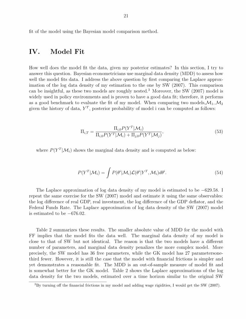
The Laplace approximation of log data density of my model is estimated to be −629.58. Irepeat the same exercise for the SW (2007) model and estimate it using the same observables:the log difference of real GDP, real investment, the log difference of the GDP deflator, and theFederal Funds Rate. The Laplace approximation of log data density of the SW (2007) modelis estimated to be −676.02.

Table 2 summarizes these results. The smaller absolute value of MDD for the model withFF implies that the model fits the data well. The marginal data density of my model isclose to that of SW but not identical. The reason is that the two models have a differentnumber of parameters, and marginal data density penalizes the more complex model. Moreprecisely, the SW model has 36 free parameters, while the GK model has 27 parametersone-third fewer. However, it is still the case that the model with financial frictions is simpler andyet demonstrates a reasonable fit. The MDD is an out-of-sample measure of model fit andis somewhat better for the GK model. Table 2 shows the Laplace approximations of the logdata density for the two models, estimated over a time horizon similar to the original SW

3By turning off the financial frictions in my model and adding wage rigidities, I would get the SW (2007).

22

Table 2: Marginal Data Density Test

Model comparison my model SW (2007)

Laplace approximation of Log data density -629.58 -676.02Number of shocks 6 7Number of observables 4 4Number of Estimated Parameters 25 36Number of Fixed Parameters 6 5

(2007) sample (1962Q1-2004Q4). I also estimate the model for a period that encompassesthe latest financial crisis (1962Q1-2010Q4);4 the results regarding relative predictive powerremain unchanged. This confirms the reasonable fit of the model with financial frictions. Moregenerally, the sample period that I use includes several periods of financial stress or crisis.Having a measure of financial stress, such as the spread between lending and borrowing, enablesmy model to capture the impact of a financial crisis in a more direct and efficient way. The SWmodel captures these effects through the second round impact on real and nominal variables.The other feature of the model with financial friction that leads to this result is the presenceof financial shocks, which are closely related to the countercyclical spread. In an economywithout financial frictions, an exogenous drop in quality of capital stock harms the capitalaccumulation process and increases the rate of depreciation; this will eventually lower outputmodestly. However, in the presence of financial frictions, a negative capital quality shockaffects the economy through an additional channel, namely the bank balance sheet, by creatinga significant capital loss in the financial sector. Section 6 provides more in-depth microeconomicinterpretations of such financial shocks.

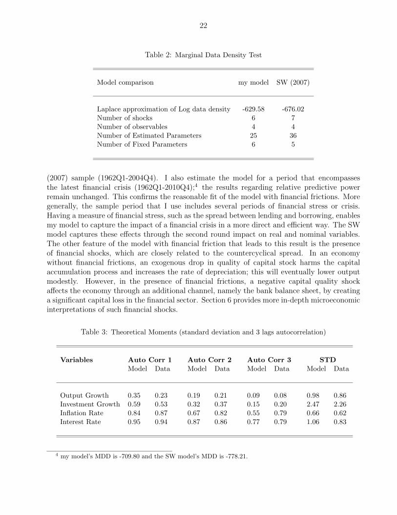
Table 3: Theoretical Moments (standard deviation and 3 lags autocorrelation)

Variables Auto Corr 1 Auto Corr 2 Auto Corr 3 STDModel Data Model Data Model Data Model Data

Output Growth 0.35 0.23 0.19 0.21 0.09 0.08 0.98 0.86Investment Growth 0.59 0.53 0.32 0.37 0.15 0.20 2.47 2.26Inflation Rate 0.84 0.87 0.67 0.82 0.55 0.79 0.66 0.62Interest Rate 0.95 0.94 0.87 0.86 0.77 0.79 1.06 0.83

4 my model’s MDD is -709.80 and the SW model’s MDD is -778.21.

23

Next, I compare a set of statistics implied by the model to those measured in the data.In particular, I cross compare theoretical moments of estimated variables with the observablevariables used for the estimation. Table 3 reports the standard deviation and three lags au-tocorrelation coefficients of the observable variables included in the estimation, namely outputgrowth, investment growth, inflation rate, and interest rate. One can observe from Table 3 thatthe estimation matches the moments in the data relatively well.

V. Drivers of Business Cycle

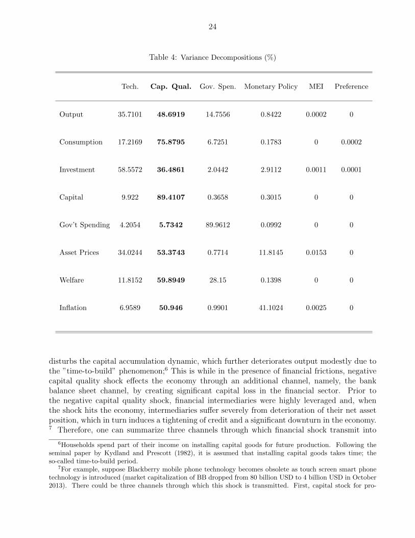
Investment shocks have proven quite successful in explaining long-run growth and have beenadopted as a standard feature of many DSGE models. Following Papanikolao (2011), invest-ment shocks change the resource cost of producing new capital goods and, thus, through theEuler equation, have an effect on consumption and output. In the New Keynesian DSGEmodel of JPT (2010), without financial frictions, analysis of variance decomposition shows thatbusiness cycles are driven primarily by shocks that affect the transformation of investmentgoods into installed capital (MEI shocks), rather than the transformation of consumption intoinvestment goods (IST shocks). In my model, the presence of financial frictions provides a suit-able framework for emphasizing, first, the role of interest rate spread and, second, the wedgebetween MEI shocks and financial shocks in explaining the US business cycle. The variancedecompositions of variables in the model are computed.5 Table 4 reports the contribution ofthe four most important shocks in the model to the variance of macroeconomic variables atbusiness cycle frequencies. The first result to stress is that MEI processes play virtually no rolein business cycles, after introducing financial shocks into the model.

The second result that emerges from Table 4 is that capital quality shocks are the key driversof business cycle fluctuations. They are responsible for 49, 75, 36, 62, and 60 percent of thevariance of output, consumption, investment, spread, and welfare, respectively. The remarkablefeature of the model that leads to these results is the close relationship between financial shocksand countercyclical credit spread. A financial shock in this model is the shock which affects thequality of productive capital stock, and it is highly correlated with the spread. Hence, policieswhich affect the credit spread are the most effective instruments in aiding recovery during fi-nancial distress. Both results are in favor of JPT (2010), as the common feature of both modelsis the importance of the shocks which are correlated with the credit spread. In addition, I goone step further and decompose the financial shock from the MEI.

Presence of capital quality shock is the novel feature of the GK (2011) model. As it is arguedthere, in an economy without financial frictions, a negative shock to the quality of capital stock

5The results are qualitatively robust over different estimation sample sizes: 1962Q1-1985Q4, 1986Q1-2004Q4,and 1962Q1-2010Q4.

24

Table 4: Variance Decompositions (%)

Tech. Cap. Qual. Gov. Spen. Monetary Policy MEI Preference

Output 35.7101 48.6919 14.7556 0.8422 0.0002 0

Consumption 17.2169 75.8795 6.7251 0.1783 0 0.0002

Investment 58.5572 36.4861 2.0442 2.9112 0.0011 0.0001

Capital 9.922 89.4107 0.3658 0.3015 0 0

Gov’t Spending 4.2054 5.7342 89.9612 0.0992 0 0

Asset Prices 34.0244 53.3743 0.7714 11.8145 0.0153 0

Welfare 11.8152 59.8949 28.15 0.1398 0 0

Inflation 6.9589 50.946 0.9901 41.1024 0.0025 0

disturbs the capital accumulation dynamic, which further deteriorates output modestly due tothe ”time-to-build” phenomenon;6 This is while in the presence of financial frictions, negativecapital quality shock effects the economy through an additional channel, namely, the bankbalance sheet channel, by creating significant capital loss in the financial sector. Prior tothe negative capital quality shock, financial intermediaries were highly leveraged and, whenthe shock hits the economy, intermediaries suffer severely from deterioration of their net assetposition, which in turn induces a tightening of credit and a significant downturn in the economy.7 Therefore, one can summarize three channels through which financial shock transmit into

6Households spend part of their income on installing capital goods for future production. Following theseminal paper by Kydland and Prescott (1982), it is assumed that installing capital goods takes time; theso-called time-to-build period.

7For example, suppose Blackberry mobile phone technology becomes obsolete as touch screen smart phonetechnology is introduced (market capitalization of BB dropped from 80 billion USD to 4 billion USD in October2013). There could be three channels through which this shock is transmitted. First, capital stock for pro-

25

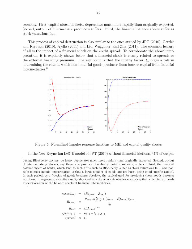
economy. First, capital stock, de facto, depreciates much more rapidly than originally expected.Second, output of intermediate producers suffers. Third, the financial balance sheets suffer asstock valuations fall.

This process of capital destruction is also similar to the ones argued by JPT (2010), Gertlerand Kiyotaki (2010), Ajello (2011) and Liu, Waggoner, and Zha (2011). The common featureof all is the impact of a financial shock on the credit spread. To corroborate the above inter-pretation, it is explicitly shown below that a financial shock is closely related to spreads orthe external financing premium. The key point is that the quality factor, ξ, plays a role indetermining the rate at which non-financial goods producer firms borrow capital from financialintermediaries.8

5 10 15 20 25 30 35 40−1

−0.8

−0.6

−0.4

−0.2

0

0.2

0.4

0.6

0.8

1

Investment Shock (M.E.I.)

Equity

Output

5 10 15 20 25 30 35 40

−1.6

−1.4

−1.2

−1

−0.8

−0.6

−0.4

−0.2

0

Capital Quality Shock

Price of Capital

Output

Figure 5: Normalized impulse response functions to MEI and capital quality shocks

In the New Keynesian DSGE model of JPT (2010) without financial frictions, 37% of output

ducing Blackberry devices, de facto, depreciates much more rapidly than originally expected. Second, outputof intermediate producers, say those who produce Blackberry parts or software, suffers. Third, the financialbalance sheets of banks, which lend to such firms such as Blackberry, suffer as stock valuations fall. One pos-sible microeconomic interpretation is that a large number of goods are produced using good-specific capital.In each period, as a fraction of goods becomes obsolete, the capital used for producing those goods becomesworthless. In aggregate, a capital quality shock reflects the economic obsolescence of capital, which in turn leadsto deterioration of the balance sheets of financial intermediaries.

8

spreadt+1 = (Rk,t+1 −Rt+1)

Rk,t+1 =Pmt+1α

Yt+1

Kt+1+ (Qt+1 − δ(Ut+1))ξt+1

Qt

Rt+1 = (βΛt,t+1)−1

spreadt+1 = at+1 + bt+1ξt+1

spreadt ∝ ξt

26

variation and 79% of investment volatility are explained by the marginal efficiency of investmentshocks, while the TFP shock is the second most significant. In an economy with informationasymmetry, where the spread between borrowing and lending is non-zero, costly state verifi-cation puts in place a mechanism to monitor the risk in banks’ activities. A deterioration ofquality of productive capital adversely affects output and demand for productive capital, low-ers good producer firm’s stock valuation and their collateral value, and, ultimately, financialintermediaries’ asset valuation in their balance sheets drops. As is shown in the above figure,a capital quality shock implies a procyclical price of capital. On the other hand, a marginalefficiency of investment shock implies that the value of net worth (or the stock market equity) iscountercyclical. This is the main reason that, in the presence of the financial accelerator block,the data favors the capital quality shock over the marginal efficiency of investment shock.

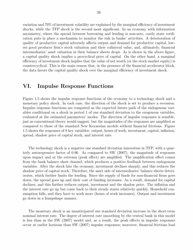
VI. Impulse Response Functions

Figure 1.5 shows the impulse response functions of the economy to a technology shock and amonetary policy shock. In each case, the direction of the shock is set to produce a recession.Impulse response functions are computed as the expected future path of the endogenous vari-ables conditional on a shock in period 1 of one standard deviation to the exogenous variables,evaluated at the estimated parameters’ modes. The direction of impulse responses is sensible,just as conventional theory would suggest, but the magnitudes of the responses are amplified ascompared to those of the standard New Keynesian models without financial frictions. Figure1.5 shows the responses of 8 key variables: output, hours of work, investment, capital, inflation,spread, shadow price of capital stock, and interest rate.

The technology shock is a negative one standard deviation innovation in TFP, with a quar-terly autoregressive factor of 0.96. As compared to SW (2007), the magnitude of responsesupon impact and at the extrema (peak effect) are amplified. The amplification effect comesfrom the bank balance sheet channel, which produces a positive feedback between endogenousvariables. After the shock hits the economy, investment declines sharply, and this reduces theshadow price of capital stock. Therefore, the asset side of intermediaries’ balance sheets deteri-orates, which further limits the lending. Since the supply of funds for non-financial firms goesdown, the spread goes up and their cost of funding increases. As a result, demand for capitaldeclines, and this further reduces output, investment and the shadow price. The inflation andthe interest rate go up but come back to their steady states relatively quickly. Household con-sumption falls, and they have to work more (hours of work increases). Output and investmentgo down in a humpshape manner.

The monetary shock is an unanticipated one standard deviation increase in the short-termnominal interest rate. The degree of interest rate smoothing by the central bank in this modelis less than in the SW (2007) model and, as a result, the peak effects in impulse responsesoccur at earlier horizons than SW (2007) impulse responses; moreover, financial frictions lead

27

5 10 15 20 25 30 35 40

−0.8

−0.6

−0.4

−0.2

% ∆

SS

Output

Tech

MP

5 10 15 20 25 30 35 40

−2

−1

0

Investment

% ∆

SS

5 10 15 20 25 30 35 40−0.4

−0.2

0

0.2

0.4

Hours

% ∆

SS

5 10 15 20 25 30 35 40

−0.6

−0.4

−0.2

Capital

% ∆

SS

5 10 15 20 25 30 35 40

−0.2

−0.1

0

0.1

Inflation

% ∆

SS

5 10 15 20 25 30 35 40

−0.05

0

0.05

0.1

Interest Rate

% ∆

SS

5 10 15 20 25 30 35 40

0

0.02

0.04

0.06

0.08

Spread

% ∆

SS

5 10 15 20 25 30 35 40

−0.6

−0.4

−0.2

0

Asset Price

% ∆

SS

Figure 6: Impulse responses to technology (blue) and monetary policy (red) shocks

to amplification in responses due to the strongly countercyclical premium. In line with SW(2007)’s findings the peak effect of a policy shock on inflation occurs before its peak effect onoutput.

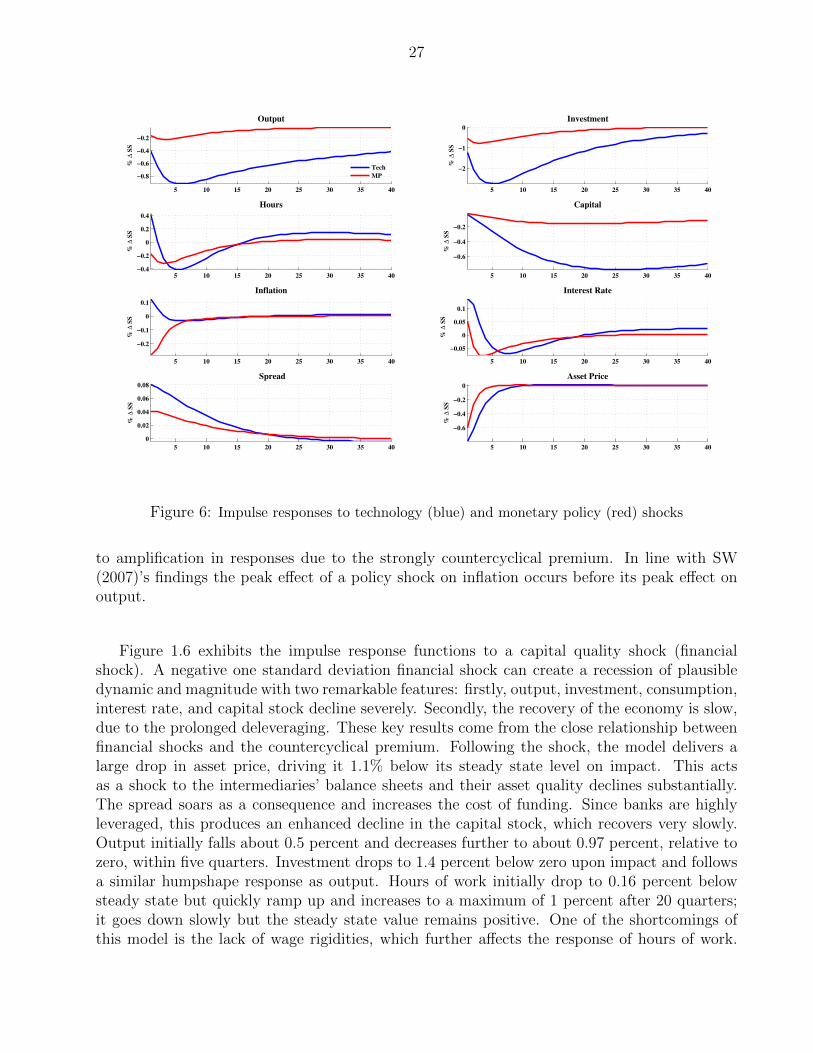
Figure 1.6 exhibits the impulse response functions to a capital quality shock (financialshock). A negative one standard deviation financial shock can create a recession of plausibledynamic and magnitude with two remarkable features: firstly, output, investment, consumption,interest rate, and capital stock decline severely. Secondly, the recovery of the economy is slow,due to the prolonged deleveraging. These key results come from the close relationship betweenfinancial shocks and the countercyclical premium. Following the shock, the model delivers alarge drop in asset price, driving it 1.1% below its steady state level on impact. This actsas a shock to the intermediaries’ balance sheets and their asset quality declines substantially.The spread soars as a consequence and increases the cost of funding. Since banks are highlyleveraged, this produces an enhanced decline in the capital stock, which recovers very slowly.Output initially falls about 0.5 percent and decreases further to about 0.97 percent, relative tozero, within five quarters. Investment drops to 1.4 percent below zero upon impact and followsa similar humpshape response as output. Hours of work initially drop to 0.16 percent belowsteady state but quickly ramp up and increases to a maximum of 1 percent after 20 quarters;it goes down slowly but the steady state value remains positive. One of the shortcomings ofthis model is the lack of wage rigidities, which further affects the response of hours of work.

28

5 10 15 20 25 30 35 40

−0.9

−0.8

−0.7

−0.6

−0.5

Output

% ∆

SS

5 10 15 20 25 30 35 40

−2

−1

0

Investment

% ∆

SS

5 10 15 20 25 30 35 40

−0.2

0

0.2

0.4

0.6

0.8

Hours

% ∆

SS

5 10 15 20 25 30 35 40

−2.5

−2

−1.5

−1

−0.5

Capital

% ∆

SS

5 10 15 20 25 30 35 40

−0.15

−0.1

−0.05

0

Inflation

% ∆

SS

5 10 15 20 25 30 35 40

−0.3

−0.2

−0.1

0

Interest Rate

% ∆

SS

5 10 15 20 25 30 35 40

0

0.05

0.1

Spread

% ∆

SS

5 10 15 20 25 30 35 40

−1

−0.5

0

Asset Price

% ∆

SS

Figure 7: Impulse responses to capital quality shock

Therefore, to get a more accurate response of hours, one would need to include appropriate labormarket imperfections in the model. Recovery of the economy is slow and in line with evidencefrom the recent financial crisis. During this period, the intermediary sector is deleveragingby building up equity relative to assets. It is widely known that banking crises preceded bycredit bubbles are typically followed by prolonged deleveraging. Data shows that the averagedeleveraging period is 5 to 6 years and typically starts 2 years after the onset of a financialcrisis. 9 It is clear from impulse responses that output recovery occurs only after 6 quartersand it takes 5 years for it to return to the pre-crisis steady state.

VII. Conclusion

I developed a New Keynesian DSGE model which features endogenous market friction, basedon the model of Gertler and Karadi (2011), with financial shocks and marginal efficiency ofinvestment shocks. The model parameters are estimated using a Bayesian technique. The fitof the model is further assessed by comparing the marginal data density (MDD) of the modelwith the frictionless economy described in Smets and Wouters (2007).I found that a Bayesianmodel comparison would pick the model with financial frictions over the baseline frictionless

9McKinsey ”Episodes of Deleveraging.”

29

model.

This paper further studies the sources of business cycle fluctuations in the spirit of Jus-tiniano, Primiceri, and Tambalotti (2010). The presence of financial frictions in my modelprovides a framework which emphasizes the role of the credit spread and the wedge betweenmarginal efficiency of investment shocks and financial shocks in explaining the US businesscycle. The analysis of variance decomposition shows that with the presence of financial inter-mediaries explicitly in the model, financial shocks are the predominant source of variability inkey macroeconomic variables at business cycle frequencies. A key conclusion of this paper isthat policies that reduce the costs associated with financial transactions would be most effectivein facilitating economic recovery. Moreover, when analyzing the impact of economic policies onbusiness cycle developments, it would be essential to use macroeconomic models that explicitlyincorporate a financial sector.

30

References

[1] Ajello, A., 2010. Financial intermediation, investment dynamics and business cycle fluctu-ations (MPRA Paper No. 32447). University Library of Munich, Germany.

[2] Bernanke, B., Gertler, M., 1989. Agency Costs, Net Worth, and Business Fluctuations.American Economic Review 79, 1431.

[3] Bernanke, B.S., Gertler, M., Gilchrist, S., 1999. The financial accelerator in a quantitativebusiness cycle framework (Handbook of Macroeconomics). Elsevier.

[4] Calvo, G.A., 1983. Staggered prices in a utility-maximizing framework. Journal of MonetaryEconomics 12, 383398.

[5] Carlstrom, C.T., Fuerst, T.S., 1997. Agency Costs, Net Worth, and Business Fluctuations:A Computable General Equilibrium Analysis. American Economic Review 87, 893910.

[6] Christiano, L., Motto, R., Rostagno, M., 2013. Risk Shocks (NBER Working Paper No.18682). National Bureau of Economic Research, Inc.

[7] Dib, A., Christensen, I., 2005. Monetary Policy in an Estimated DSGE Model with a Fi-nancial Accelerator (Computing in Economics and Finance 2005 No. 314). Society for Com-putational Economics.

[8] Foerster, A.T., 2011. Financial crises, unconventional monetary policy exit strategies, andagents expectations (Research Working Paper No. RWP 11-04). Federal Reserve Bank ofKansas City.

[9] Gertler, M., Gilchrist, S., 1993. The Role of Credit Market Imperfections in the MonetaryTransmission Mechanism: Arguments and Evidence. Scandinavian Journal of Economics95, 4364.

[10] Gertler, M., Karadi, P., 2011. A model of unconventional monetary policy. Journal ofMonetary Economics 58, 1734.

[11] Gertler, M., Kiyotaki, N., 2010. Financial Intermediation and Credit Policy in BusinessCycle Analysis (Handbook of Monetary Economics). Elsevier.

[12] Giannone, D., Reichlin, L., Sala, L., 2005. Monetary Policy in Real Time (NBER Chap-ters). National Bureau of Economic Research, Inc.

[13] Gilchrist, S., Yankov, V., Zakrajsek, E., 2009. Credit market shocks and economic fluctu-ations: Evidence from corporate bond and stock markets. Journal of Monetary Economics56, 471493.

[14] Greenwood, J., Hercowitz, Z., Krusell, P., 1997. Long-Run Implications of Investment-Specific Technological Change. American Economic Review 87, 34262.

31

[15] Greenwood, J., Hercowitz, Z., Huffman, G. 1988. Investment, Capacity Utilization, andthe Real Business Cycle, American Economic Review, American Economic Association,American Economic Association, vol. 78(3), pages 402-17, June.

[16] Hirakata, N., Sudo, N., Ueda, K., 2011. Do banking shocks matter for the U.S. economy?Journal of Economic Dynamics and Control 35, 20422063.

[17] Iacoviello, M., 2005. House Prices, Borrowing Constraints, and Monetary Policy in theBusiness Cycle. American Economic Review 95, 739764.

[18] Justiniano, A., Primiceri, G.E., Tambalotti, A., 2010. Investment shocks and businesscycles. Journal of Monetary Economics 57, 132145.

[19] Kiyotaki, N., Moore, J., 1997. Credit Cycles. Journal of Political Economy 105, 21148.

[20] Kiyotaki, N., Moore, J., 2012. Liquidity, Business Cycles, and Monetary Policy (NBERWorking Paper No. 17934). National Bureau of Economic Research, Inc.

[21] Kydland, F. E, Prescott, E. C., 1982. Time to Build and Aggregate Fluctuations, Econo-metrica, Econometric Society, Econometric Society, vol. 50(6), pages 1345-70, November.

[22] Liu, Z., Waggoner, D.F., Zha, T., 2011. Sources of macroeconomic fluctuations: Aregimeswitching DSGE approach. Quantitative Economics 2, 251301.

[23] Mandelman, F.S., 2010. Business cycles and monetary regimes in emerging economies: Arole for a monopolistic banking sector. Journal of International Economics 81, 122138.

[24] Nolan, C., Thoenissen, C., 2009. Financial shocks and the US business cycle. Journal ofMonetary Economics 56, 596604.

[25] Papanikolaou, D., 2011. Investment Shocks and Asset Prices. Journal of Political Economy119, 639 685.

[26] Primiceri, G., 2005. Why Inflation Rose and Fell: Policymakers Beliefs and US PostwarStabilization Policy (NBER Working Paper No. 11147). National Bureau of Economic Re-search, Inc.

[27] Roxburgh, C., Lund, S., Wimmer, T., Amar, E., Atkins, C., Kwek, J., Dobbs, R., Manyika,J. 2011. Debt and deleveraging: The global credit bubble and its economic consequences.McKinsey Report

[28] Sannikov, Y., Brunnermeier, M.K., 2010. A Macroeconomic Model with a Financial Sector(2010 Meeting Paper No. 1114). Society for Economic Dynamics.

[29] Sims, C.A., 2002. Solving Linear Rational Expectations Models. Computational Economics20, 120.

[30] Smets, F., Wouters, R., 2007c. Shocks and Frictions in US Business Cycles: A BayesianDSGE Approach. American Economic Review 97, 586606.

32

A Appendix - Data

output = LN( GDPC96 / LNSindex ) * 100investment = LN( ( FPI / GDPDEF ) / LNSindex ) * 100inflation = LN( GDPDEF / GDPDEF(-1) ) * 100interest rate = Federal Funds Rate / 4

GDPC96 : Real Gross Domestic Product - Billions of Chained 1996 Dollars, Seasonally AdjustedAnnual Rate. Source: US Department of Commerce, Bureau of Economic Analysis

GDPDEF : Gross Domestic Product - Implicit Price Deflator - 1996=100, Seasonally Adjusted.Source: US Department of Commerce, Bureau of Economic Analysis

FPI : Fixed Private Investment - Billions of Dollars, Seasonally Adjusted Annual Rate. Source:US Department of Commerce, Bureau of Economic Analysis

Federal Funds Rate : Averages of Daily Figures - Percent. Source: Board of Governors of theFederal Reserve System.

LFU800000000 : Population level - 16 Years and Older - Not Seasonally Adjusted. Source: USBureau of Labor Statistics

LNS10000000 : Labor Force Status : Civilian noninstitutional population - Age : 16 years andover- Seasonally Adjusted - Number in thousands. Source: US Bureau of Labor Statistics. (Before1976 : LFU800000000 : Population level - 16 Years and Older)