Financial Development, Economic Growth And Poverty In Kenya
275
FINANCIAL DEVELOPMENT, ECONOMIC GROWTH AND POVERTY IN KENYA ISABEL NYAMBURA WAIYAKI A THESIS SUBMITTED IN PARTIAL FULFILLMENT FOR THE DEGREE OF DOCTOR OF PHILOSOPHY IN ECONOMICS IN THE SCHOOL OF ECONOMICS, UNIVERSITY OF NAIROBI. November, 2016
Transcript of Financial Development, Economic Growth And Poverty In Kenya

FINANCIAL DEVELOPMENT, ECONOMIC GROWTH AND POVERTY IN
KENYA
ISABEL NYAMBURA WAIYAKI
A THESIS SUBMITTED IN PARTIAL FULFILLMENT FOR THE DEGREE OF
DOCTOR OF PHILOSOPHY IN ECONOMICS IN THE SCHOOL OF
ECONOMICS, UNIVERSITY OF NAIROBI.
November, 2016

i
DECLARATION
This thesis is my original work and has not been presented for a degree award in any other
university.
ISABEL WAIYAKI DATE
X80/91906/2013
_______________________ _________________
This thesis has been submitted for examination with our approval as university
supervisors:
DR. PETER MURIU (Ph.D) DATE
SCHOOL OF ECONOMICS, UNIVERSITY OF NAIROBI
_______________________ _________________
PROF. NELSON WAWIRE (Ph.D) DATE
SCHOOL OF ECONOMICS, KENYATTA UNIVERSITY
________________________ __________________

ii
DEDICATION
To my faithful God and my parents, Mr and Mrs Edward Waiyaki.

iii
ACKNOWLEDGEMENTS
First of all, I would like to thank the Almighty God for walking the PhD journey with me
and enabling me to complete it. Isaiah 26: 12b, ―All I have achieved is because of God‖. I
am grateful to the African Economic Research Consortium for awarding me the
scholarship to undertake my PhD studies. I am grateful to the University of Nairobi,
School of Economics and University of Dar es salaam, Department of Economics for
according me admission and taking me through the various stages of my PhD studies. I am
greatly indebted to my supervisors, Dr. Peter Muriu and Professor Nelson Wawire for their
guidance, direction, critical review and timely feedback in the various phases of my thesis
writing. I learnt a lot under their guidance.
I owe special thanks to Professor Germano Mwabu who guided me in shaping my thesis. I
thank the director School of Economics, Professor Jane Mariara for her constant moral
support during the entire time of my PhD studies. I would also like to thank Dr. Nancy
Nafula, KIPPRA for her selfless guidance on poverty data issues. Not to forget the support
accorded me by Dr. Daniel Amanja in obtaining data from Central Bank of Kenya.
I appreciate the efforts of my parents Mr. and Mrs. Edward Waiyaki for taking me to
school and sacrificing a lot for my sake, I will forever be indebted. My brothers; Charles,
Mitterrand, Anthony and Patrick, thanks for your support, prayers and encouragement. To
my precious friends Anne and George, Mercy, Nyambura, Tabitha, Fidelis, Gloria, Ndanu,
Sarah, Phyllis, Diana and Laura, your prayers, support and encouragement kept me going
even when I would threaten to quit. Finally, I cannot forget my classmates whom we
tirelessly worked with to beat deadlines in our PhD work. Special recognition to Michael
and Richard for encouraging me to always soldier on, your kindness overwhelms me.
Despite all this able assistance, the views expressed in this thesis are solely those of the
author and do not represent the views of any of the recognized person(s) or institution(s). I
therefore bear the full responsibility for any errors and/or omissions. Delighted to have put
this thesis together, I am confident that it will hone ongoing debate on financial
development, growth and poverty.
iv
ABSTRACT
It is evident that the financial sector in Kenya has grown rapidly in the last decade.
However, the economy has had a low fluctuating growth and poverty levels have remained
rampantly high. The effect of financial development on economic growth and poverty and
especially the efficiency and quality aspects of financial sector development have been
ignored. Again, Kenya‘s financial sector is more advanced compared to other African
countries but the factors explaining this disparity have not been examined. This study,
therefore, aimed at filling this research gap. The core objectives of the thesis were to
determine the drivers of financial development and to determine the effect of financial
development on economic growth and poverty. The novelity of the study findings arise
from controlling for financial innovations, using appropriate measures of financial
development and poverty incorporating the efficiency and quality aspects of financial
development. Autoregressive Distributed Lag Model, Granger causality, cointegration
analysis and Vector Error Correction Model were used for analysis using quarterly time
series data for the period 2000 to 2014.
This study found that credit to private sector model which shows level of intermediation in
the financial sector supported the openness hypothesis indicating the importance of trade
openness for financial development. The non-performing loans model which captures the
quality of credit and efficiency in the financial sector supported the economic institutions
hypothesis by stressing the importance of institutional quality for financial development.
Other key determinants were GDP, political economy and mobile technology.
Further findings showed that financial development incorporating the efficiency and
quality aspects as indicated by non-performing loans and interest rate spread had a positive
effect on economic growth. Still, financial development directly reduces poverty in Kenya
while it also indirectly reduces poverty through economic growth thus confirming the
trickle down hypothesis of growth on poverty reduction. Additionally, the recent financial
innovations were found to increase growth and also reduce poverty. The main channels
through which financial innovation contributed to growth and poverty reduction included
the transfer, credit and savings channels. Financial development was predominantly seen to
granger-cause economic growth thus supporting the supply leading hypothesis.
Based on the findings, the study made the following policy recommendations. There
should be improvement in the quality of legal, economic and political institutions by the
government. A more democratic environment with a system of political checks and
balances should be maintained. The government should have trade policies to grow the
volume of trade. Growth of financial innovations should be supported by creating a
conducive environment by the regulatory bodies, government and other institutions. The
efficiency and quality of the financial sector should be improved with interest rate reforms
to reduce the interest rate spread and reduction of non-performing loans. This ought to
include policies to monitor credit to private sector. Finally, economic growth should be
targeted through innovations and other measures like maintaining a good macro economic
environment while encouraging a more inclusive growth to reduce poverty.

v
TABLE OF CONTENTS
DECLARATION .................................................................................................................... i
DEDICATION .......................................................................................................................ii
ACKNOWLEDGEMENTS ................................................................................................. iii
ABSTRACT .......................................................................................................................... iv
LIST OF TABLES ................................................................................................................ ix
LIST OF FIGURES .............................................................................................................xii
LIST OF ABBREVIATIONS AND ACRONYMS ........................................................... xiv
DEFINITION OF TERMS ................................................................................................xvii
CHAPTER ONE .................................................................................................................... 1
INTRODUCTION ................................................................................................................. 1
1.1 Background .................................................................................................................. 1
1.2 Financial Sector Developments ................................................................................... 1
1.3.1 Mobile Money Services .......................................................................................... 15
1.3.2 The Case of M-Pesa ................................................................................................ 18
1.3.3 Relationship between Financial Development and Financial Innovation............... 24
1.4 Economic Growth ...................................................................................................... 25
1.5 Poverty status ............................................................................................................. 28
1.6 Financial Development, Economic Growth and Poverty Link .................................. 29
1.7 The Statement of the Problem.................................................................................... 31
1.8 Objectives of the Study .............................................................................................. 33
1.9 Significance of the Study ........................................................................................... 33

vi
1.10 Scope of the Study ................................................................................................... 34
1.11 Structure of the Thesis ............................................................................................. 34
CHAPTER TWO ................................................................................................................. 35
DETERMINANTS OF FINANCIAL DEVELOPMENT ................................................... 35
2.1 Introduction ................................................................................................................ 35
2.2 Literature Review....................................................................................................... 39
2.2.1 Theoretical Literature.............................................................................................. 39
2.2.2 Empirical Literature ................................................................................................ 43
2.2.3 Overview of the Literature ...................................................................................... 54
2.3 Methodology .............................................................................................................. 55
2.3.1 Theoretical Framework ........................................................................................... 55
2.3.2 Model Specification ................................................................................................ 56
2.3.3 Definition and Measurement of Variables .............................................................. 59
2.3.4 Data Type and Sources ........................................................................................... 61
2.3.5 Estimation and Testing ............................................................................................ 61
2.4 Empirical Results and Discussion .............................................................................. 66
2.5 Conclusions and Policy Implications ......................................................................... 79
2.6 Contribution of the Study........................................................................................... 82
2.7 Limitation of the Study .............................................................................................. 83
2.8 Areas for Further Research ........................................................................................ 83
CHAPTER THREE ............................................................................................................. 84
FINANCIAL DEVELOPMENT AND ECONOMIC GROWTH ....................................... 84
3.1 Introduction ................................................................................................................ 84
vii
3.2 Literature Review....................................................................................................... 87
3.2.1 Theoretical Literature.............................................................................................. 87
3.2.2 Empirical Literature ............................................................................................... 90
3.2.3 Overview of the Literature .................................................................................... 100
3.3 Methodology ............................................................................................................ 103
3.3.1 Theoretical Framework ......................................................................................... 103
3.3.2 Empirical Model ................................................................................................... 105
3.3.3 Estimation and Testing .......................................................................................... 107
3.3.4 Definition and Measurement of Variables ............................................................ 116
3.3.5 Data Set and Description ...................................................................................... 119
3.4 Empirical Results and Discussion ............................................................................ 119
3.5 Conclusions and Policy Implications .................................................................. 135
3.6 Contribution of the Study to knowledge ............................................................. 138
3.7 Limitations of the Study ...................................................................................... 139
3.8 Areas for Further Research ................................................................................. 140
CHAPTER FOUR .............................................................................................................. 141
FINANCIAL DEVELOPMENT AND POVERTY .......................................................... 141
4.1 Introduction .............................................................................................................. 141
4.2 Literature Review..................................................................................................... 146
4.2.1 Theoretical Literature............................................................................................ 146
4.2.2 Empirical Literature .............................................................................................. 147
4.2.3 Overview of Literature .......................................................................................... 158
4.3 Methodology ............................................................................................................ 159
4.3.1 Theoretical Framework ......................................................................................... 159
viii
4.3.2 Model Specification .............................................................................................. 161
4.3.3 Estimation and Testing .......................................................................................... 163
4.3.4 Definition and Measurement of Variables ............................................................ 165
4.3.5 Data Set and Description ...................................................................................... 169
4.4 Empirical Results and Discussion ............................................................................ 170
4.5 Conclusion and Policy Implications ........................................................................ 188
4.6 Contribution of the Study .................................................................................... 191
4.7 Limitations of the Study ...................................................................................... 191
4.8 Areas for Further Research ................................................................................. 192
CHAPTER FIVE ............................................................................................................... 193
SUMMARY, CONCLUSIONS AND POLICY IMPLICATIONS................................... 193
5.1 Introduction .............................................................................................................. 193
5.2 Summary of the Thesis ............................................................................................ 193
5.3 Conclusions .............................................................................................................. 195
5.4 Policy Implications .................................................................................................. 196
5.4 Contribution of the Study to Knowledge ................................................................. 200
5.5 Limitations of the Study........................................................................................... 201
5.6 Areas for further research ........................................................................................ 202
REFERENCES .................................................................................................................. 203
APPENDIX ........................................................................................................................ 235

ix
LIST OF TABLES
Table 1.1: Conversions of NBFIs into Banks ........................................................................ 5
Table 1.2: List of Banks with Crossborder Operations.......................................................... 7
Table 2.1: Definition and Measurement of Variables .......................................................... 60
Table 2.2: Descriptive Statistics .......................................................................................... 67
Table 2.3: Unit Root Tests ................................................................................................... 69
Table 2.4: Zivot-Andrews Unit Root Test Results .............................................................. 70
Table 2.5: ARDL Bounds Test ............................................................................................ 71
Table 2.6: Long-run Estimates of the Credit to Private Sector Model ................................ 72
Table 2.7: Long-run Estimates of the Non-performing Loans Model ................................. 74
Table 2.8: ECM Estimates of Credit to Private Sector and Non-performing Loans Models
.............................................................................................................................................. 77
Table 3.1: Summary of the Findings of the Relationship between Finance and Growth .... 99
Table 3.2: Definition and Measurement of Variables ........................................................ 118
Table 3.3: Phillip - Perron Unit Root Test Results ............................................................ 121
Table 3.4: Zivot Andrews Unit Root Test Results ............................................................. 122
Table 3.5: Cointegration Results with Trace Statistic ....................................................... 123
Table 3.6: Cointegration Results with Max-Eigen Statistic ............................................... 123
Table 3.7: VECM Long – run Relationship Results .......................................................... 125
Table 3.8: VECM Short – run Relationship Results .......................................................... 127
Table 3.9: Granger Causality Results of the Real GDP Model ......................................... 129
Table 3.10: Variance Decompositions of GDP to Other Variables ................................... 131
Table 3.11: Variance Decomposition of Other Variables to GDP ..................................... 132

x
Table 3.12: VECM Long–run Relationship Results Incorporating Financial Innovation . 133
Table 3.13: Short – run Relationship Results Incorporating Financial Innovation ........... 134
Table 4.1: National Poverty Rates in Kenya ...................................................................... 142
Table 4.2: Income Poverty (Percent) in Kenya by Regions: 1992-2006 ........................... 142
Table 4.3: Summary of Findings of the Effect of Financial Development on Poverty ..... 156
Table 4.4: Summary of Findings of the Relationship between Finance and Poverty ........ 157
Table 4.5: Definition and Measurement of Variables ........................................................ 169
Table 4.6: Descriptive statistics for the poverty variables ................................................. 170
Table 4.7: Phillip Perron Unit Root Test Results .............................................................. 172
Table 4.8: Zivot-Andrews Unit Root Test Results for Poverty Measures ......................... 172
Table 4.9: Johansen Test Results for the Head Count Ratio Model .................................. 173
Table 4.10: VECM Long-run Results with Head Count Ratio .......................................... 174
Table 4.11: Short-run Relationship on VECM with Head Count Ratio ............................ 176
Table 4.12: Granger Causality Results with Head Count Ratio ........................................ 179
Table 4.13: Johansen Cointegration Test Results of Per Capita Consumption Model ...... 180
Table 4.14: VECM Results – Long-run Relationship with Per Capita Consumption ....... 181
Table 4.15: VECM Results – Short-run Relationship with Per Capita Consumption ....... 185
Table 4.16: Granger Causality Test Results of the Per Capita Consumption Model ........ 187
Table A.1: Optimal Lag Length Results ............................................................................ 244
Table A.2: Short-run Regression Results of the Market Capitalization Model ................. 246
Table A.3: Correlation Matrix between GDP and Independent Variables ........................ 247
Table A.4: Clemente – Montanes – Reyes Unit Root Test Results ................................... 247
Table A.5: Optimal Lag Length Results ............................................................................ 248
Table A.6: Autocorrelation Test of the Residuals in Lag 1 Model .................................... 248
xi
Table A.7: Granger Causality Results while Controlling for Financial Innovation .......... 249
Table A.8: Post Estimation Tests Results of the GDP Model ........................................... 250
Table A.9: Sensitivity of Rural Poverty to Income Growth and Income Distribution ...... 250
Table A.10: Sensitivity of Urban Poverty to Income Growth and Income Distribution ... 250
Table A.11: Sensitivity of National Poverty to Income Growth and Income Distribution 251
Table A.12: Correlation Matrix with Per Capita Consumption ......................................... 251
Table A.13: Correlation Matrix with Head Count Ratio ................................................... 252
Table A.14: Optimal Lag Length of the Model with Per Capita Consumption ................. 252
Table A.15: LM Test of Per Capita Consumption Model at Lag Two .............................. 253
Table A.16: Optimal Lag Length of the Head Count Ratio Model ................................... 254
Table A.17: LM Test of Head Count Ratio Model at Various Lags .................................. 254
Table A.18: Post Estimation Tests Results of the Head Count Ratio Model .................... 256
Table A.19: Post Estimation Tests Results of the Per Capita Consumption Model .......... 256
Table A.20: Predicted Quarterly Head Count Ratio for the Period 2001 – 2014 .............. 257

xii
LIST OF FIGURES
Figure 1.1: Comparison of Use of Banks and Mobile Phone Financial Services ................ 15
Figure 1.2: Mobile Money Subscriptions ............................................................................ 16
Figure 1.3: Mobile Money Agents ....................................................................................... 16
Figure 1.4: No. of Agents per Mobile Money Service ........................................................ 17
Figure 1.5: Mobile Money Transactions and Volumes ....................................................... 17
Figure 1.6: No. of M-Pesa Subscriptions ............................................................................. 19
Figure 1.7: No. of M-Pesa Agents ....................................................................................... 19
Figure 1.8: M-Pesa Transactions and Volumes ................................................................... 20
Figure 1.9: M-Swari Loans and Deposits Accounts and Amounts ...................................... 21
Figure 1.10: Migration of People to the Use of Mobile Money Transfer Services ............. 23
Figure 1.11: GDP Growth Rate ........................................................................................... 26
Figure 1.12: Average Annual Growth Rates for EAC Countries for the Period 2010-2015
.............................................................................................................................................. 26
Figure 1.13: Kenya's GDP Before and After Rebasing ....................................................... 27
Figure 1.14: Poverty Trends in Kenya between 1992 and 2005 .......................................... 28
Figure 1.15: Poverty Trends Estimates in Kenya after 2006 ............................................... 28
Figure 1.16: Link between Financial Development, Economic Growth and Poverty ......... 30
Figure 2.1: Trends in Financial Development Indicators .................................................... 36
Figure 3.1: GDP and Financial Sector Growth Rates .......................................................... 85
Figure 3.2: Causality between Real GDP and Financial Development Indicators ............ 130
Figure 4.1: Relationship between Financial Sector Growth and Poverty Rates ................ 143
Figure A.1: Relationship between M-Pesa Agents and Credit to Private Sector............... 235
Figure A.2: Relationship between M-Pesa Agents and Non-Performing Loans (NPL) .... 235
xiii
Figure A.3: Relationship between M-Pesa Agents and M3 ............................................... 236
Figure A.4: Relationship between M-Pesa Agents and Bank Deposits ............................. 236
Figure A.5: Trend in Real GDP ......................................................................................... 237
Figure A.6: Trend in Credit to Private Sector .................................................................... 237
Figure A.7: Trend in Interest Rate Spread ......................................................................... 238
Figure A.8: Trend in Non-perfoming Loans ...................................................................... 238
Figure A.9: Trend in Market Capitalization ...................................................................... 239
Figure A.10: Trend in Interest Rate Spread ....................................................................... 239
Figure A.11: Trend in Trade Openness.............................................................................. 240
Figure A.12: Trend in GDP Per Capita .............................................................................. 240
Figure A.13: Trend in Head Count Ratio........................................................................... 241
Figure A.14: Trend in Per Capita Consumption ................................................................ 241
Figure A.15: Trend in Democratic Accountability ............................................................ 242
Figure A.16: Trend in Institutional Quality ....................................................................... 242
Figure A.17: Trend in Remittances .................................................................................... 243
Figure A.18: Trend in Technology .................................................................................... 243
Figure A.19: Cusum of Squares Parameter Stability of Credit to Private Sector Model ... 245
Figure A.20: Cusum of Squares Parameter Stability of Non-perfoming Loans Model ..... 245
Figure A.21: Cusum of Squares Parameter Stability of Market Capitalization Model ..... 246
Figure A.22: Stability of the Real GDP VECM model with Two Lags ............................ 249
Figure A.23: Stability of the Per Capita Consumption VECM Model with Two Lags ..... 253
Figure A.24: Stability of the Head Count Ratio VECM Model with Two Lags ............... 255
Figure A.25: Stability of the Head Count Ratio VECM Model with Three Lags ............. 255
Figure A.26: Stability of the Head Count Ratio VECM Model with Four Lags ............... 256

xiv
LIST OF ABBREVIATIONS AND ACRONYMS
ADF: Augmented Dickey-Fuller
AERC: African Economic Research Consortium
AFC: Agricultural Financial Corporation
AIMS: Alternative Investment Market Segment
ARDL: Autoregressive Distributed Lag
CBK: Central Bank of Kenya
CMA: Capital Markets Authority
CPS: Credit to Private Sector
DCP: Domestic Credit to Private Sector
EABS: East African Building Society
EAC: East African Community
ECT: Error Correction Term
ECM: Error Correction Model
ECB: Equatorial Commercial Bank
FI: Financial Intermediation
FD: Financial Development
FIMS: Fixed Income Market Segment
FSD: Finacial Sector Deepening
GOK: Government of Kenya

xv
GDP: Gross Domestic Product
GCC: Gulf Cooperation Council
GLS: Generalized Least Squares
GMM: Generalized Method of Moments
ICDC: Industrial and Commercial Development Corporation
IDB: Industrial Development Bank
IMF: International Monetary Fund
IRA Insurance Regulatory Authority
IRF: Impulse Response Functions
KIHBS: Kenya Integrated Household Budget Survey
KNBS Kenya National Bureau of Statistics
MDG: Millenium Development Goals
MIMS: Main Investment Market Segment
MKT: Market Capitalization
MLE: Maximum Likelihood Estimation
MNO: Mobile Network Operator
MSE: Micro and Small Enterprises
NBFI: Non-Bank Financial Institution
NPEP: National Poverty Eradication Plan
NPL: Non-Performing Loans

xvi
NSE: Nairobi Securities Exchange
OECD: Organization for Economic Cooperation and Development
OLS: Ordinary Least Squares
PCA: Principal Components Analysis
PP: Phillip-Perron
PRSP: Poverty Reduction Strategy Paper
SACCO: Savings and Credit Co-operative Society
SAP: Structural Adjustment Program
VAR: Vector Auto-regressive
VECM: Vector Error Correction Model

xvii
DEFINITION OF TERMS
Financial Development: The creation and expansion of financial institutions and
instruments, growth in financial services as well as enhancement in the policies that
improve intermediation, stability and efficiency. This is extended to include the qualitative
and effiency aspects.
Financial Innovation: The introduction of new financial instruments and products or the
implementation of new ideas or financial technologies for the betterment of a system.
Economic Growth: An increase in output or GDP of a country over time.
Poverty: Inability to meet life‘s basic needs.
Head Count Ratio: The number of the poor that live below the poverty line to total
population.
Poverty Line: Minimum level of income necessary for basic living and below which one is
considered poor.
M3: M1 plus M2 and long term time deposits, institutional money market funds and
repurchase agreements.
M2: Short term time deposits and individual money market funds.
M1: Currency in circulation and other money equivalents easily convertible to cash.
Credit to Private Sector: Credit extended by the banking industry to the private sector in an
economy.
Market capitalization: Value of all outstanding shares of all companies listed at the Nairobi
Stock exchange.
Non-performing Loans: Sum of loans for which the borrowers have not made payment for
atleast 90 days.
1
CHAPTER ONE
INTRODUCTION
1.1 Background
Financial development is the creation and expansion of institutions, financial instruments
and markets as well as the policies and factors that lead to efficient and effective
intermediation in the growth process (FitzGerald, 2006). Further, financial innovation is a
component of financial development and can be defined as the creation and advancement
of financial instruments, products (product innovation), institutions (institutional
innovation) and processes (process innovation). In a narrow sense, it can be defined as
introduction of new financial instruments and products or the implementation of new ideas
or instruments for the betterment of a system (Blach, 2011). The financial system in Kenya
is developing and this chapter discusses some of the main aspects of growth in the
financial system.
Moreover, the theoretical link between finance and growth shows that financial
development may impact growth and poverty through the Mckinnon (1973), ―conduit
effect‖ where increase in savings increases investment. This link is further explained by the
endogenous growth theories. Financial development may also impact on poverty directly
or indirectly through economic growth. There is also a debate in the literature trying to
confirm these relationships and this study delves into these relationships introducing new
concepts. This chapter further introduces discussions on growth and poverty particularly in
the recent past in Kenya using available data.
1.2 Financial Sector Developments
Kenya‘s financial sector has been outstanding in its performance relative to other
economies in Sub Saharan Africa (Alter and Yontcheva, 2015). The relatively well
developed financial sector consists of: the Central Bank of Kenya (CBK), 43 Commercial
Banks, one Mortgage Finance Company, 12 deposit taking micro finance institutions, eight
2
representatives of foreign banks, 86 foreign exchange bureaus, three credit reference
bureaus, one Post Office Savings Bank, about 300 Savings and Credit Co-operative
Societies, 38 Insurance Companies, the Nairobi Securities Exchange and Venture Capital
Companies, National Social Security Fund (NSSF) and pension funds (CBK, 2014b).
The financial sector has seen a lot of innovations and developments including growth in
the banking sector, capital markets, insurance industry and other financial instruments
innovations. The banks have grown to 43 with some institutions changing from
microfinance institutions to banks and major banks going cross-border mostly in the entire
East African region. There is also more trading among banks. The Nairobi Securities
Exchange has grown and it has attracted a lot of diaspora funds (NSE, 2014). In 2014, the
net inflows stood at Kshs. 3.5 million which increased to Kshs. 5.7 million in 2015 (NSE,
2015).
1.2.2 Developments in the Banking Sector
The banking sector is the most advanced in East Africa to date (Alter and Yontcheva,
2015). Only about 29.2 percent of the population had access to banking services in 2013
(FSD et al., 2013). Kimenyi and Ndungu (2009) had shown that about 20 to 30 percent of
the population had access to banking services in 2009 and thus the situation had not
changed much by 2013.
The financial sector has experienced a number of banking crises. In 1986, Union Bank and
a few Non-Banking Financial Institutions (NBFIs) like Rural Urban Credit Finance Bank
Limited collapsed. To deal with the problem, eight financial institutions were taken over
and merged into a state bank in 1989; Consolidated Bank of Kenya Limited. In 1993, the
Exchange bank was closed due to the Goldenberg scandal (a corruption case where the
government paid a company, Goldenberg international 35 percent more than their foreign
currency earnings). In 1998, four banks collapsed due to poor management. They included:
Trust Bank, Reliance Bank, Prudential Bank and Bullion Bank while National bank almost
3
collapsed as well. By then, two multinational banks-the Standard Chartered Bank and
Barclays Bank of Kenya; and the locally owned banks-Kenya Commercial Bank and
National Bank of Kenya dominated the banking sector. The total assets of Kenya‘s six
largest banks (Kenya Commercial Bank Limited, National Bank of Kenya, Barclays Bank
(K) Limited, Standard Chartered (K) Limited, Cooperative Bank of Kenya and Equity
Bank (K) Limited) increased from US $2.8 billion in 1997 to US $ 12.1 billion in 2013,
representing about half (51.3 percent) of the total assets of all commercial banks (CBK,
2014b). By 2015, this had increased to US $ 18.15 billion which is about 50 percent of the
total assets of all commercial banks which is still very high (CBK, 2015). The Central
Bank has strengthened the supervision and inspection of banks with quarterly and annual
supervision reports being produced. It has also introduced a Deposit Protection Fund which
guarantees deposits of up to one hundred thousand Kenya Shillings. The initial capital for
setting up financial institutions has been increased for commercial banks and ―specified‖
NBFIs.
Commercial banks have expanded in number and also increased their assets. The locally
incorporated banks increased steadily in the 1990s with the deliberate government effort to
increase local ownership of financial institutions. The locally incorporated commercial
banks did not compare well with the foreign counterparts in their assets levels. Most of
them had less than the average asset level as compared with foreign banks. But the local
banks continued to take an increasing share in the market. To ensure competition and
mitigation from failures as well as ensure that they met the core capital requirements of the
CBK, banks have been merging. Typical examples include: Southern Credit and Equatorial
commercial bank merged in 2007, Commercial Bank of Africa Limited merged with
American Bank Kenya Limited in 2005 retaining the name Commercial Bank of Africa
Limited while Biashara bank Limited was acquired by Investment & Mortgage Bank Ltd
in 2003. The Banking Act, 2015 allows banks to have shareholders hold only 25 percent of
their share capital. New rules which may be set for banks may see a lot of changes. There
was a suggestion by the CBK to raise the core capital requirement for banks to five (5)
4
billion Kenya shillings up from one (1) billion Kenya shillings in 2016. Although this was
not effected, if it was to be, it would affect the tier III banks with a few of tier II banks
which have a core capital of less than 5 billion Kenya Shillings including K-rep bank (tier
II), Habib, Oriental, Equatorial Commercial, United Bank of Africa, Guarantee Trust bank
(CBK, 2014b). This would lead to an increase in mergers if the banks are not able to raise
the capital by raising the shareholders funds or selling equity stakes through Initial Public
Offerings (IPOs).
A lot of developments have been realized in the banking sector for the last 10 years. This
has been characterized by transformations of NBFI‘s to bank and introduction of new
products like Automated Teller Machines (ATMs). In 2004, the CBK reduced the retention
ratio from 6 percent to 5 percent which released credit to the economy making loans more
affordable. Over time, the CBK has controlled the amount of credit in the economy
through reserves and Central Bank rate. However, banks had previously ignored the
Central Bank rate in setting their base lending rates motivated by their desire to make more
profits. There is the Banking amendment Act, 2016 which is being discussed by the
Parliament of Kenya which proposes interest rate caps. These caps would be set at upto
four percentage points above the Central Bank Rate for lending rates and minimum of 70
percent of Central Bank Rate for deposits. Banks had too many requirements for opening
an account and other transactions and this kept many people financially excluded. In 2005,
Equity Bank Limited which transformed into a bank from a NBFI reduced its requirements
for opening accounts and accessing loans thus creating a lot of competition for the other
banks and increasing financial access to the unbanked. Since 1994, many Non-Banking
Financial Institutions have transformed into banks as illustrated by Table 1.1.
5
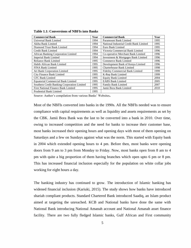
Table 1.1: Conversions of NBFIs into Banks
Commercial Bank Year Commercial Bank Year
Universal Bank Limited 1994 Paramount Bank Limited 1995
Akiba Bank Limited 1994 National Industrial Credit Bank Limited 1995
Diamond Trust Bank Limited 1994 Euro Bank Limited 1995
Credit Bank Limited 1994 Victoria Commercial Bank Limited 1996
African Banking Corporation Limited 1994 Co-operative Merchant Bank Limited 1996
Imperial Bank Limited 1994 Investment & Mortgages Bank Limited 1996
Reliance Bank Limited 1995 Commerce Bank Limited 1996
Habib African Bank Limited 1995 Development Bank of Kenya Limited 1996
FINA Bank Limited 1995 Charterhouse Bank Limited 1998
Ari Bank Corporation Limited 1995 Fidelity Commercial Bank Limited 1999
City Finance Bank Limited 1995 K-Rep Bank Limited 1999
CFC Bank Limited 1995 Equity Bank Limited 2004
Equatorial Commercial Bank Limited 1995 EABS Bank Limited 2005
Southern Credit Banking Corporation Limited 1995 Family Bank Limited 2007
First National Finance Bank Limited 1995 Jamii Bora Bank Limited 2010
Prudential Bank Limited 1995
Source: Author‘s compilation from various Banks‘ Websites.
Most of the NBFIs converted into banks in the 1990s. All the NBFIs needed was to ensure
compliance with capital requirements as well as liquidity and assets requirements as set by
the CBK. Jamii Bora Bank was the last to be converted into a bank in 2010. Over time,
owing to increased competition and the need for banks to increase their customer base,
most banks increased their opening hours and opening days with most of them opening on
Saturdays and a few on Sundays against what was the norm. This started with Equity bank
in 2004 which extended opening hours to 4 pm. Before then, most banks were opening
doors from 9 am to 3 pm from Monday to Friday. Now, most banks open from 8 am to 4
pm with quite a big proportion of them having branches which open upto 6 pm or 8 pm.
This has increased financial inclusion especially for the population on white collar jobs
working for eight hours a day.
The banking industry has continued to grow. The introduction of Islamic banking has
widened financial inclusion (Kariuki, 2015). The study shows how banks have introduced
shariah compliant products. Standard Chartered Bank introduced Saadiq, an Islam product
aimed at targeting the unreached. KCB and National banks have done the same with
National Bank introducing National Amanah account and National Amanah asset finance
facility. There are two fully fledged Islamic banks, Gulf African and First community
6
Banks. Both were licensed by CBK in 2007. The banks have introduced Shariah compliant
banking products like Sukuks (Islamic bonds) and Muraabahah1. Other banks have
introduced Islamic banking units after being cleared by CBK. These include: Barclays
Bank, Standard Chartered Bank, Chase Bank, KCB and Middle East Bank (CBK, 2014b).
Integration of ATMs by small Micro finance institutions has also seen its way in the
banking sector. It involves customers withdrawing funds from any pesa pay2 ATMs and
not necessarily an ATM belonging to one‘s specific bank. This has contributed to financial
depth by increasing velocity of money. In 2010, the cheque truncation project was
introduced. It is a system in which cheque clearing takes one day as opposed to previous
times when the process took four days. This system was operationalized in August 2011.
The introduction of Credit Information Sharing (CIS) in July 2010 which has seen
establishment of three credit reference bureaus has strengthened the credit appraisal
standards and reduced risks of non-performing loans for banks since both negative and
positive information of borrowers is shared (CBK, 2014a). So far, the non-performing
loans as a percentage of total loans have remained below the 10 percent mark.
Agency banking has also been introduced into the banking industry which is a
diversification strategy aimed at taking banking services closer to the people. It was
introduced in May 2010 after the CBK publicized prudential guidelines on agent banking
and by January 2011, banks had already started using agency banking. Agency banking
allows banks to use various outlets like shopping malls, supermarkets, mobile Telco
agents, petrol stations, chemists, dry cleaners and other CBK approved business to act as
bank agents in areas where banks lack presence. By March 2013, agency banking
transactions cumulatively stood at $ 3 Billion (CBK, 2013b). As at that time, there were 11
commercial banks which had contracted over 18,082 agents. This has increased to $ 3
1Muraabahah – a product where the bank buys an asset upon request by client from a third party and resells
to the client
2 Cash withdrawal

7
Billion in 2015 (For example, KCB started KCB Mtaani3 in 2011 opening up its first agent
in Embakasi area. Equity was the first bank to start agency banking while Postbank
followed suit with its Postbank Mashinani4. Co-operative Bank of Kenya in 2013 started
its Co-op kwa Jirani5 agencies as part of competition with other banks which had started
agency banking. Other banks that have embraced agency banking include Family Bank
with its Pesapap agent service and Chase Bank with chase popote6. Agency banking allows
services like cash deposits, cash withdrawals, transfer payments, school fees payments,
utility payments, balance enquiry, Mobile phone airtime top up, mini-statements and other
banking services (CBK, various bank supervision reports).
Banks have also gone cross border over time looking for business in neighbouring
countries in the whole of East African region. Table 1.2 shows crossborder banking.
Table 1.2: List of Banks with Crossborder Operations
Bank Country of Operations Year of establishment
Kenya Commercial Bank Tanzania
South Sudan
Uganda
Rwanda
Burundi
1997
2006
2008
2009
2012
Co-operative Bank Tanzania
Uganda
2004
2012
Equity Bank Uganda and South Suda
Rwanda
Tanzania
2008
2011
2012
NIC Bank Tanzania
Uganda
2004
2012
CFC-Stanbic Bank South Sudan 2013
Commercial Bank of Africa Tanzania
Uganda
2007
2013
Family Bank South Sudan 2013
Source: Author‘s compilation from various banks‘ websites.
3Mtaani – a Swahili word meaning town
4Mashinani – meaning deep in the village
5Jirani – meaning neighbour
6Popote – meaning everywhere
8
Many of the Kenyan owned banks have opened subsidiary banks mainly in the wider East
African region as shown in Table 1.2. In addition, they have adopted borderless banking
where customers having accounts in a bank in one country can transact in other countries
in the subsidiary bank. The motivation to do cross border banking is to tap onto customers
abroad and win customers who transact businesses in other countries. Cross border
banking also comes with many gains including competition, increased financial deepening
as well as financial stability (Beck et al., 2014). This is especially beneficial with the
opening up of the East African Community removing barriers to trade. This is likely to
lead to increased business for the banks.
Some other reasons why banks have gone cross-border include high competition in the
local market and weak market power, low institutitonal quality, increased efficiency due to
regional expansion and high inflation in the local market (Kodongo et al., 2012).
Furthermore, most of the banks have their shares cross listed in the various securities
exchanges in the region (East Africa). For example, shares of Equity Bank Limited are
traded at Nairobi Securities Exchange (NSE) while cross listed at Uganda securities
Exchange (USE), KCB‘s shares are traded at the NSE while crosslisted at USE, Rwanda
Stock Exchange (RSE) and Dar es Salaam Stock Exchange (DSE).
There have also been several policy developments in the banking sector. One is the agency
banking guidelines introduced in 2011 to give guidance to the operations of agency
banking. Moreover, the Central bank came up with revised Prudential and Risk
Management Guidelines for the banking sector to guide their operations in terms of
liquidation, setting up of representative offices of foreign banks and consumer protection.
This also included new guidelines on transfer risks and introduction of information
technology communication.
9
1.2.3 Developments in the Capital Market
The capital market comprises of the stock (equity) market and the bond (debt) market. The
Nairobi Securities Exchange (NSE) was incorporated under the Companies Act of Kenya
in 1991 as a company limited by guarantee and without a share capital. Prior to 1991, it
was registered as a voluntary association of stockbrokers under the Societies Act in 1954.
Currently, fourteen (14) stockbrokers and three (3) investment banks form the membership
of the NSE. NSE is categorized into three market segments: Main Investment Market
Segment (MIMS) which is the main quotation market, Alternative Investment Market
Segment (AIMS) which provides an alternative method of raising capital to small, medium
sized and young companies (NSE, 2014).
Fixed Income Market Segment (FIMS) on the other hand provides an independent market
for fixed income securities such as treasury bonds, corporate bonds, preference shares and
debenture stocks. Between the years 2000 and 2010, the NSE has experienced robust
activity and high returns on investment. It accounts for over 90 percent of market activity
in the East African region (World Bank, 2002) and is a reference point in terms of setting
standards for the other markets in the region.
The stock market in Kenya is currently the second largest in Africa after South Africa‘s in
terms of market capitalization and it is also ranked fifth on market liquidity (World Bank,
2013b). The Nairobi Securities Exchange‘s (NSE) growth in the last 10 years has been
phenomenon. This started with an increase in the trading hours in 2006 to 3 hours up from
2 hours and later the introduction of the Automated Trading System. In 2006 also, the NSE
entered into a MOU with Uganda Securities Exchange to allow cross listing. This has
allowed many companies‘ shares to be crosslisted not only in the two securities exchanges
but also in the wider East African region securities exchanges. For example, Kenya
Airways, Centum Company Limited, Uchumi Supermarket, KCB and Equity Bank are all
crosslisted at Uganda Securities Exchanges.

10
In 2008, the Nairobi Securities Exchange All Shares Index (NASI) was introduced which
is an overall indicator of market performance. In November 2009, automated trading of
government bonds through the ATS was introduced. This was a way of improving the
depth of capital market by increasing market liquidity (Simiyu et al., 2014). Later in
November 2011, two other indices were introduced into the NSE i.e. FTSE NSE Kenya 15
Index and the FTSE NSE Kenya 25 Index as a way of enhancing diversification in the
wider East African region. These are indices used for measuring the performance of the
companies listed at the NSE and also the performance of the major industries and capital
segments of the NSE. This was in addition to the existing indices including NSE All Share
Index, NSE 20 Share Index, FTSE NSE Kenya Government Bond Index and FTSE ASEA
Pan African Index (NSE, 2014).
In January 2013, NSE introduced a trading platform for SMEs, Growth Emerging Markets
Segments (GEMS) thus accommodating SMEs at the stock market. GEMS allow SMEs
flexible listing requirements and thus act as an alternative source of capital for SMEs
instead of the expensive bank loans. This is expected to contribute to increased liquidity
for the SMEs thereby improving financial inclusion with the number of SMEs growing
each year (NSE, 2013).
The CMA has developed the futures markets by facilitating the NSE to develop the futures
and options market. The development includes derivatives for equity and debt instruments.
Some of the products for offer include interest rate futures and foreign exchange
derivatives. Interest rate futures are beneficial to institutions which rely on
borrowing/financing to hedge against higher interest rates while foreign exchange futures
are important for sectors that rely on foreign exchange to hedge against currency risks.
These foreign exchange derivatives cuts across the major macro economic sectors of the
economy like sectors dealing with exports and imports.

11
The Electronic Trading Platform also known as the Automated Trading System (ATS) was
introduced in 2012 (NSE, 2012). The ATS allows trading immobilized corporate bonds
and treasury bonds. It has reduced cycle time and increased opening times for NSE and
orders to be queued up properly (Simiyu et al., 2014). It has also had strong consolidation
of customer accounts and CDSC avoiding poor trading at the NSE. Furthermore, it has
helped registrars in rolling out dividends in the shortest time possible. With all these
developments, the NSE is likely to attract a lot of diaspora funds as well as international
funds due to good performance. Kenya‘s NSE ASI was ranked the third best performing
stock exchange market indicator in the world after Venezuelan‘s and Egypt‘s (Osoro and
Jagongo, 2013).
Another major development is the Kenya infrastructure bonds. The first infrastructure
bond was issued in 2009 and raised 18.5 Billion shillings for roads, energy, water and
irrigation sectors. Other infrastructure bonds include the 12-year twenty billion Kenya
Shillings infrastructure bond issued in September, 2013 which was oversubscribed (CMA,
2013). Buying these infrastructure bonds has become easy for the general population as it
is not restricted to only those with CDSC accounts at the CBK. Anyone can buy through
having a CDSC account with various banks. This has opened up the infrastructure bond
market and thus increased financial inclusion.
1.2.4 Developments in the Insurance Industry
Insurance penetration in Kenya is about 3.2 percent (IRA, 2015) which is considered to be
high by African standards. The Kenyan insurance market has grown at an average of 16
percent for the last five years. In the last two years, the insurance market has recorded
about Kenya shillings 135 Billion and 158 Billion in Gross Domestic Premiums in 2013
and 2014 respectively. The market comprises of 45 insurance companies and 140
insurance brokers hence creating high levels of competition in the industry (Insurance
Regulatory Authority, 2014). Some of the developments that have happened in the
insurance industry include the micro insurance schemes like the weather-index micro
12
insurance scheme introduced in 2009. This has seen farmers being cushioned from
financial disaster arising from weather changes. A policy framework paper has been
developed by the IRA micro insurance working group with regard to micro insurance and
it awaits approval by government. Insurance companies have also embraced technology
and work with the Mobile Network Operators in introducing new products. For example,
CIC Insurance introduced a platform called M-BIMA which is an insurance package for
proprietors of M-Pesa shops. In 2011, the first Islamic Shariah compliant, fully fledged
insurance company was introduced, Takaful insurance of Africa launched by CIC
insurance group. This has increased insurance penetration especially to the Muslim
population.
1.2.5 Other Financial Sector Developments
Other developments in other financial institutions include what is commonly known as
consumer to consumer (C2C) and consumer to business (C2B) or business to consumer
(B2C). C2C occurs where the banks play a background role in linking consumers to other
consumers (the bank acts as a collection bank). The bank links consumers to other
consumers through a paybill number. The effect of this is that the banks hold onto large
sums of money for overnight lending and at the same time it reduces risks such as fraud
and others associated with handling cash by the institutions. The overall effect is that the
number of transactions has increased where consumers do not have to actually visit the
bank. Examples of these include Kenya Power and Lighting Company (KPLC) electricity
bills where consumers pay their bills through a paybill number. Both the bill payer and
KPLC happen to be consumers of the banking services but through the paybill number,
neither has to visit the bank. Other examples include payment of Higher Education Loans
Board (HELB) loans by former university students through a paybill number. C2B on the
other hand is where the consumer (individuals) creates some form of value and businesses
pick up or buy this value; commonly known as collected demand. This stimulates demand
and consumption in the economy. In the financial sector, one example of this is the M-Pesa
business which created and collected demand for money transfer.

13
Kenya‘s mortgage industry has witnessed an impressive growth in the last couple of years
due to a high demand for real estate. The mortgage market increased the number of houses
from 7,600 houses in 2006 to 20,000 houses in 2012 (World Bank, 2013b). However, the
market has been hit by the high interest rates and thus growth has been dampened. The
value of mortgage loan assets outstanding increased from Kshs 122.2 billion in 2012 to
Kshs 188.2 billion in December 2014 (CBK, 2014b). These mortgage loans are mainly
from the four main banks (KCB, Standard Chartered bank, Barclays Bank, CFC Stanbic
Bank) and a mortgage company (Housing Finance Company Limited). The activity in the
mortgage market is dependent of interest rates as well as other macro-economic variables
like inflation. In addition, access to long term funds is a major determinant of mortgage
market growth.
1.3 Financial Innovations in Kenya
There are three types of financial innovations. They include process, product and
institutional innovation. Process innovation involves the introduction of new business
processes or ways of doing things which lead to increased efficiency and higher output.
Institutional innovation includes creation of new financial intermediaries, new business
structures as well as changes in the financial, legal and regulatory framework. Examples
would include establishment of bank agents. Product innovation involves the introduction
of new financial products for example, credit, hire purchase and insurance products (Blach,
2011).
Kenya has experienced a continued growth in financial innovations and financial
developments in the last decade. Examples of some of the innovations include process
innovation like the use of ATMs, debit and credit cards and introduction of the Kenya
Electronic Payments and Settlement System (KEPSS) as well as the Automated Trading
System (ATS) in the capital markets, product innovation including use of paper money like
cheques, plastic money, introduction of Shariah compliant products like Sukuks (Islamic
bonds) and Muraabahah and finally institutional innovation which include agency banking,

14
internet banking and mobile banking. These innovations have been supported by
technological advancement and mobile money by the reduction of costs in
telecommunication. In addition, products which suit the Islamic population have been
introduced. Islamic bonds known as Sukuks were introduced in 2012 as well as new ways
of purchasing and holding assets by the Muslim community known as Muraabahah.
Institutional innovation has also become evident in Kenya with introduction of mobile
banking, internet banking and agency banking. With internet banking, people are able to do
banking from the internet without necessarily going to the bank. This has been overtaken
by mobile banking where people use their phones to do banking even without internet
connection. Further, agency banking was introduced in 2010 with the aim of taking
banking services closer to the people. With it came the agency banking Act, 2011 which
governs the use of agency banking. Banks can use various outlets stores as agents and this
has the potential of reaching more people. Many banks including Equity bank, KCB bank,
Co-operative bank, Chase bank, Post bank are all using agency banking and they have used
it as a competitive strategy to woe customers in the market.
One innovation which is drawing attention in Kenya and in the world at large from many
stakeholders including users, countries which may want to replicate and researchers is the
mobile money transfer service, M-Pesa. The system has been one of the most developed
and successful systems in the world (Jack and Suri, 2011 and Buku and Meredith, 2013)
and is considered the world leader in mobile money (Nyamongo and Ndirangu, 2013).
Since its onset, M-Pesa has grown and has attracted a number of other competitors but it
still remains the leading mobile payment system in Kenya. M-Pesa has greatly increased
financial inclusion in Kenya and has been beneficial to the poor population especially in
rural areas with limited access to banking services (FSD et al., 2013). M-Pesa is used by
over 70 percent households in Kenya out of which 50 percent are not in the banking
system while 41 percent live in the rural areas (Reed at al., 2013). Financial inclusion had

15
risen to 67 percent and 75 percent with growth of M-Pesa by the end of 2013 (FSD et al.,
2013) and 2016 (FSD et al., 2016) respectively.
1.3.1 Mobile Money Services
Aker (2010) found that over 60 percent of Africans have access to mobile phones and this
contribute greatly to the use of mobile banking. The use of mobile money in Kenya has
grown with various forms of mobile payments by Mobile Network Operators (MNOs) and
various banks. Various mobile money products include M-Pesa (launched in 2007) which
is a mobile phone based money transfer service initiated by Safaricom Limited (a Mobile
Network Operator), Airtel Money (launched in 2011) which is the equivalent of M-Pesa
for Bharti Airtel Kenya Limited, an Indian Multinational telecommunications service
company, Yu cash (launched in 2009), the equivalent for Essar Telecom Kenya Limited,
Orange money (introduced in 2010), the equivalent for Telkom Kenya Limited and
Mobikash, a mobile money service for Mobikash Kenya Limited. It is a subsidiary of
Mobicom Africa Limited which offers mobile money transfer services across all networks,
banks and biller merchants. The percentage of the Kenyan population with access to
mobile money services was 63 percent in 2014 (Communications Commission of Kenya,
2014). Majority of Kenyans have now turned to the use of mobile phone financial services
(mobile money services) as compared to the use of banking financial services. This is
shown in Figure 1.1.
Figure 1.1: Comparison of Use of Banks and Mobile Phone Financial Services
Source: FSD et al. (2016)

16
In 2013, those using mobile phone services were 63 percent in 2013 and 71.4 percent in
2016 compared to those using banks which were 29 percent in 2013 rising to 38.4 percent
in 2016 (FSD et al., 2016). Use of mobile phone services have grown at a higher rate than
use of banks. The increase in bank use is attributed to mobile banking. The number of
people subscribed to mobile money services has grown as shown in Figure 1.2.
Figure 1.2: Mobile Money Subscriptions
Source: Central Bank of Kenya (2014a)
The total number of subscriptions to mobile money services had grown from one million
subscribers in 2007 to about 26.6 Million subscribers in 2014. The growth of mobile
money service in Kenya was made successful by the use of agents. The CBK through its
Banking Act, 2013 allows agents to register and operate for example M-Pesa shops.
Mobile transfer agents have grown since the introduction of M-Pesa in 2007. This is shown
in Figure 1.3.
Figure 1.3: Mobile Money Agents
Source: Central Bank of Kenya (2014b)

17
At the onset of mobile money services, only 1,582 agents were available in December
2007. The number of agents had grown to about 123, 703 by December 2014 (CBK, 2014).
This growth is an indication that people are willing to take up mobile money services as a
form of banking in areas where banking services are limited or non-existent as well as use
it as a form of carrying money instead of having to go to the banks in areas where banks
are available. The agents were distributed among the various mobile money services as
shown in Figure 1.4
Figure 1.4: No. of Agents per Mobile Money Service
Source: Communications Authority of Kenya (2014)
Safaricom‘s M-Pesa had the most agents in the country with other networks having less
than 10,000 each. This shows the dominance of M-Pesa in Kenya. Figure 1.5 demonstrates
how mobile money services have increased between 2007 and 2014.
Figure 1.5: Mobile Money Transactions and Volumes
Source: Central Bank of Kenya (2014a)

18
Mobile money transfers grew from KShs. 5.4 Million transactions in December 2007 to
Kshs 911 Million transactions by December 2014. In addition, the volume of the mobile
money transfers increased from Kshs. 16.3 Billion in December 2007 to Kshs 2.37 Trillion
in December 2014 (CBK, 2014).
1.3.2 The Case of M-Pesa
M-Pesa7 which was introduced in 2007 is a short form of Mobile Money and it is a mobile-
phone based money transfer and micro financing service for Safaricom Limited, a Mobile
Network Operator in Kenya (and Vodacom in Tanzania). It is an innovative payment
system for the unbanked. At the moment, it is the most developed and successful mobile
payment system in the world (Buku and Meredith, 2013). M-Pesa allows customers to send
and receive money through their mobile phones. With M-Pesa, Safaricom Limited accepts
deposits from registered users. In exchange, the users receive e-float which is held in the
user‘s electronic account. This e-money is then used by users for various services
including sending, receipt and withdrawal of funds, pay bill and buy good services under
the Lipa na M-Pesa service, airtime purchase and transfer of money to bank accounts.
Other services offered include; Bank to M-Pesa where customers can withdraw money
from their bank accounts by using M-Pesa and Cashless distribution for various companies
(for example Coca cola). Some of the services paid through the LIPA na M-Pesa include
Lipa Kodi (meaning to pay rent), utility payments and salary disbursements. This service
has been one of the most useful and easiest ways of money transfer for the poor. As Aker
and Mbiti (2010) puts it, M-Pesa has evolved from solely being a money transfer system
into a payment system and is now part of the formal financial system. Recently, banks
came up with a product which links mobile phones to bank accounts. This allows
customers to access their account balances through their mobile phones as well as deposit
7Pesa is a Swahili word meaning money
19
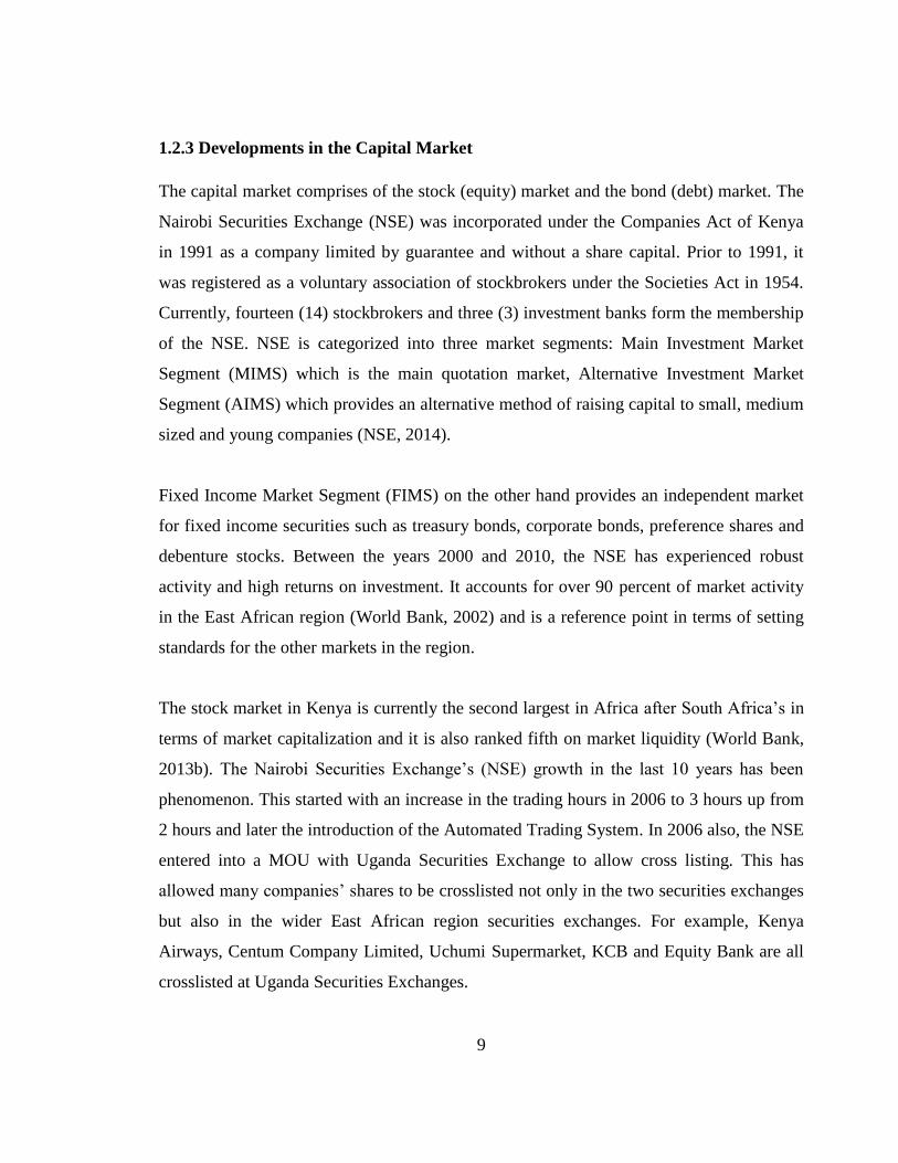
money. With all these services being offered by M-Pesa, the number of subscriptions has
increased over the years as shown in Figure 1.6.
Figure 1.6: No. of M-Pesa Subscriptions
Source: Communications Authority of Kenya (2014)
At the start of M-Pesa in 2007, only about one million of the population was subscribed to
M-Pesa but by June 2014, M-Pesa had 19.3 million users (Safaricom Limited, 2014) (over
70 percent of the adult population - Kenya Population and Housing Census Report, 2009).
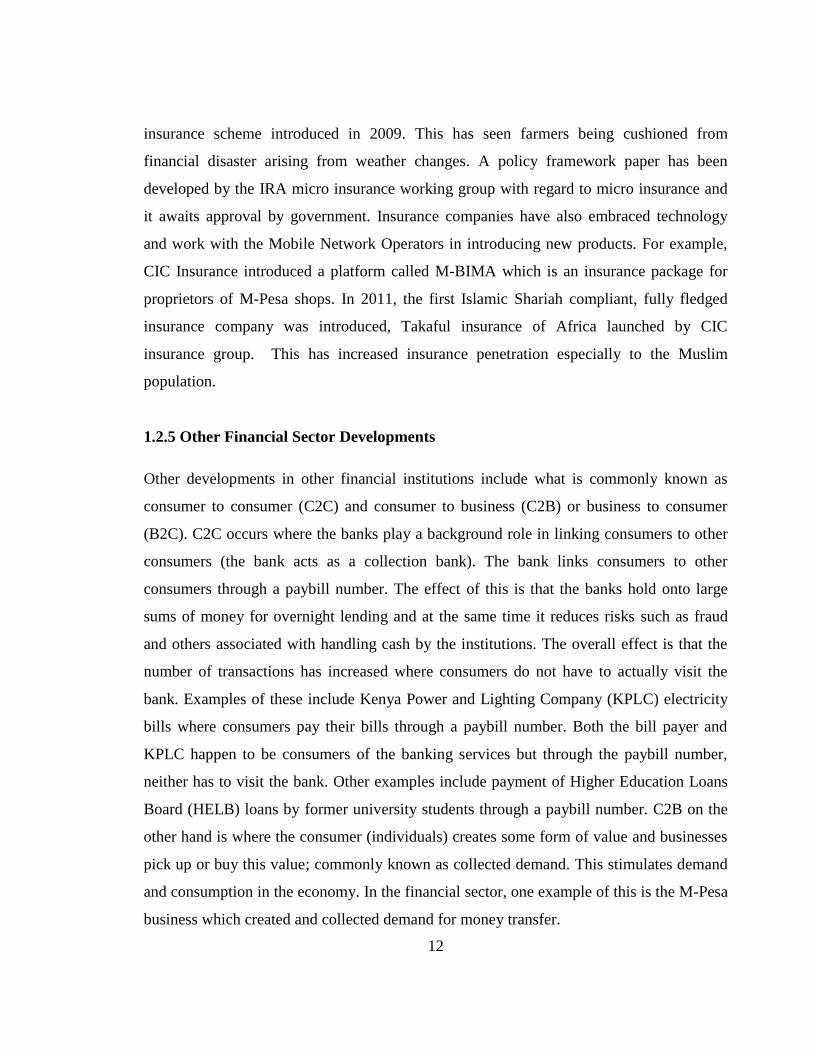
The use of M-Pesa has grown over the years with Safaricom setting up agents all over the
country to increase access. Initially, agents were concentrated in Nairobi but this later
changed with agents reaching the rural areas. Figure 1.7 shows the number of M-Pesa
agents.
Figure 1.7: No. of M-Pesa Agents
Source: Communications Authority of Kenya (2014)
20
Currently, there are over eighty thousand M-Pesa agents in the country up from only about
one thousand in June 2007. Unlike the banking system, the role of M-Pesa is to improve
financial access and not financial intermediation (Buku and Meredith, 2014). M-Pesa is
more of a transactional platform and a store of value system. M-Pesa transaction flows
account for about 43 percent of GDP (Safaricom, 2015) which gives the unbanked access
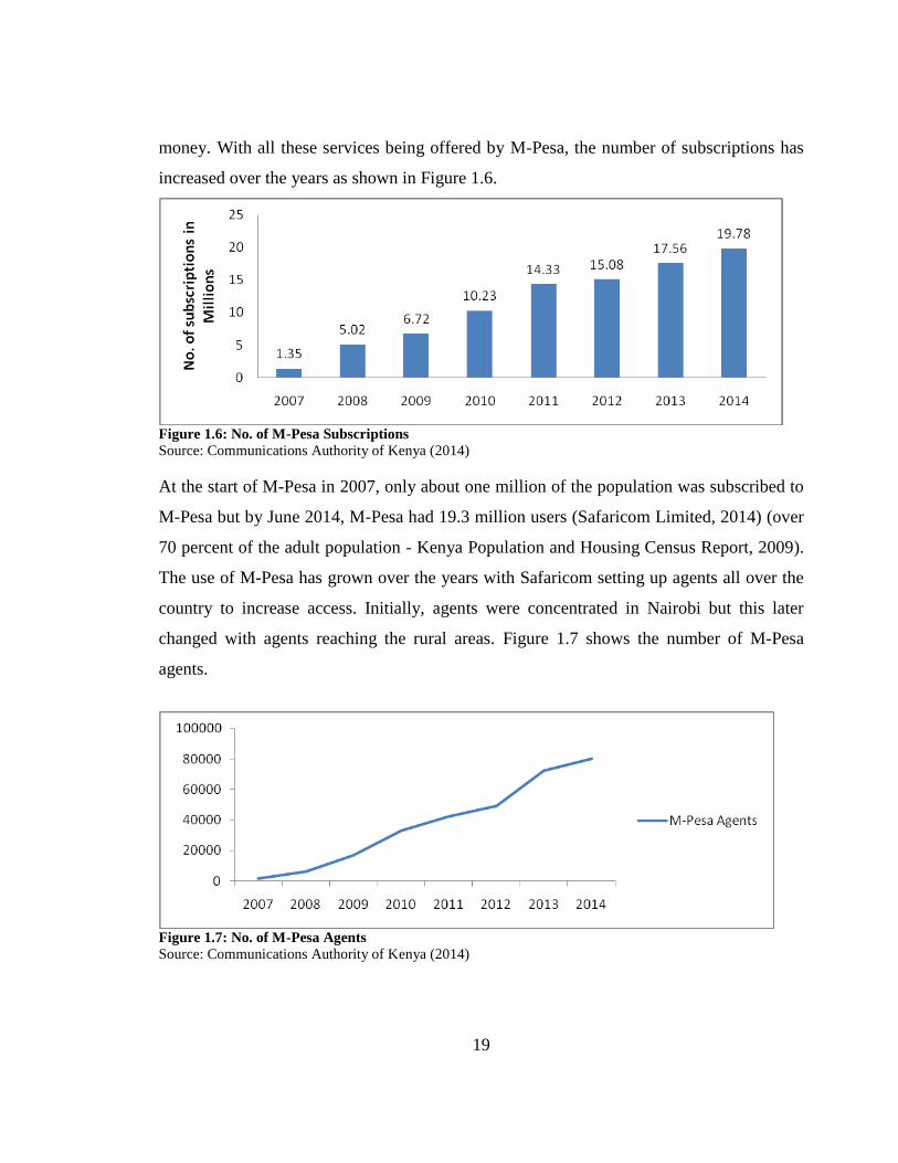
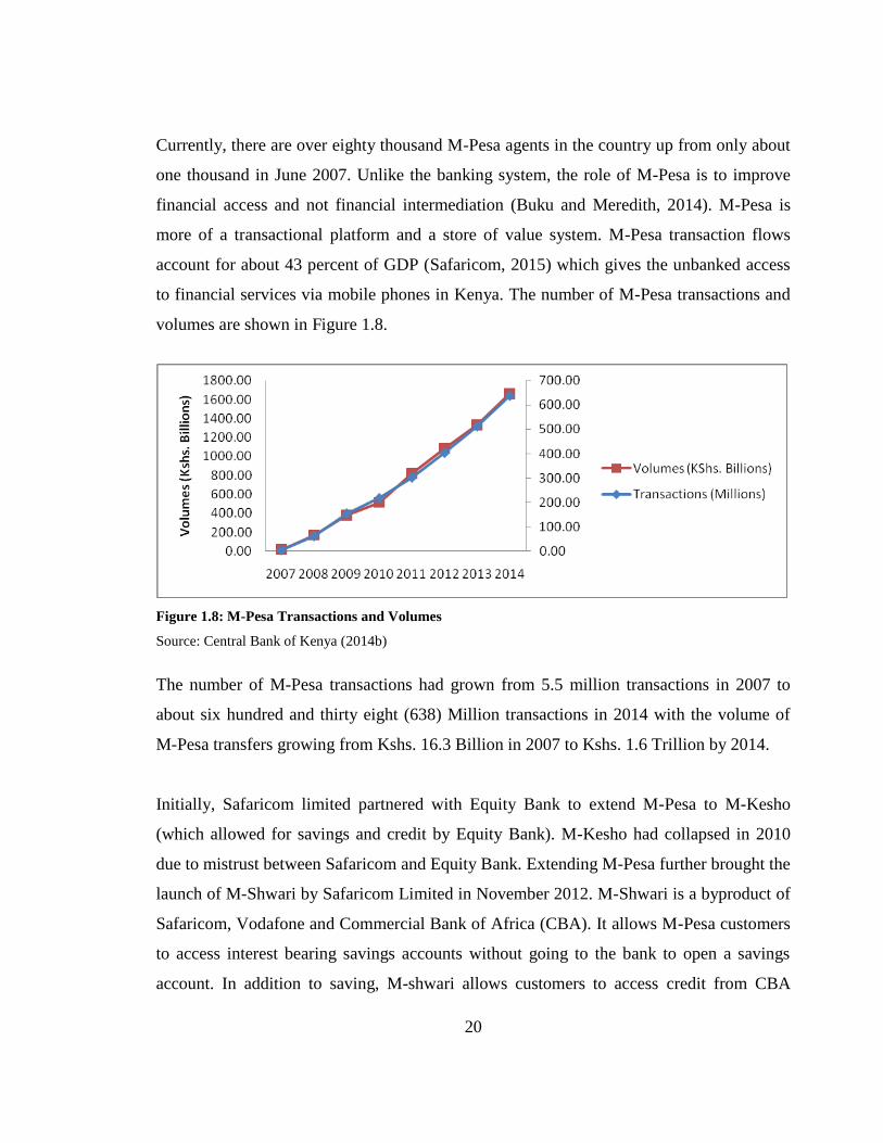
to financial services via mobile phones in Kenya. The number of M-Pesa transactions and
volumes are shown in Figure 1.8.
Figure 1.8: M-Pesa Transactions and Volumes
Source: Central Bank of Kenya (2014b)
The number of M-Pesa transactions had grown from 5.5 million transactions in 2007 to
about six hundred and thirty eight (638) Million transactions in 2014 with the volume of
M-Pesa transfers growing from Kshs. 16.3 Billion in 2007 to Kshs. 1.6 Trillion by 2014.
Initially, Safaricom limited partnered with Equity Bank to extend M-Pesa to M-Kesho
(which allowed for savings and credit by Equity Bank). M-Kesho had collapsed in 2010
due to mistrust between Safaricom and Equity Bank. Extending M-Pesa further brought the
launch of M-Shwari by Safaricom Limited in November 2012. M-Shwari is a byproduct of
Safaricom, Vodafone and Commercial Bank of Africa (CBA). It allows M-Pesa customers
to access interest bearing savings accounts without going to the bank to open a savings
account. In addition to saving, M-shwari allows customers to access credit from CBA
21
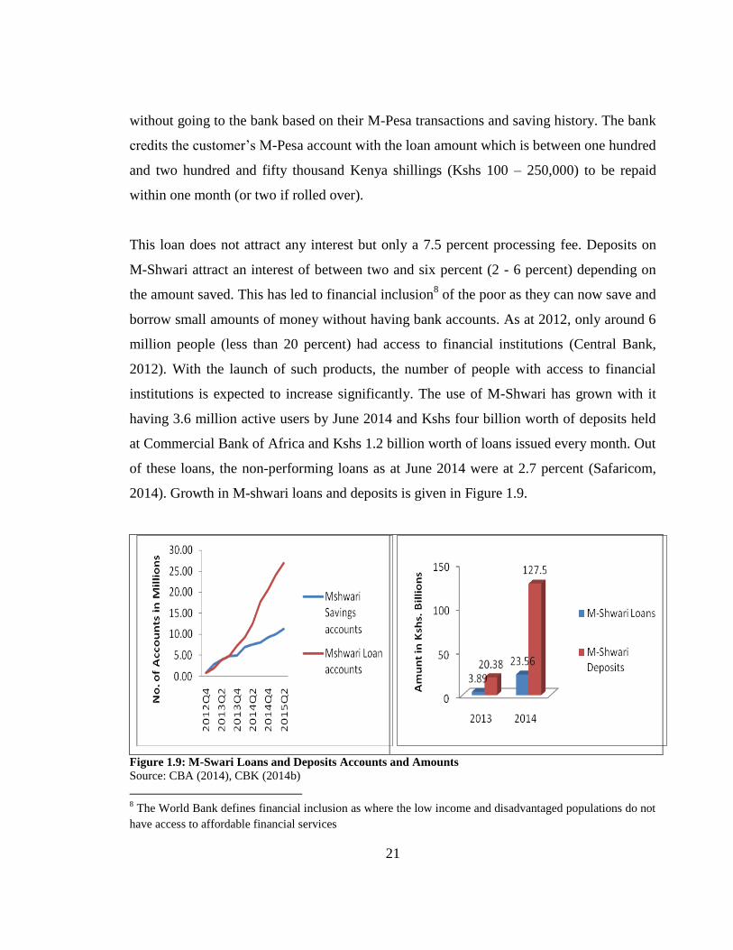
without going to the bank based on their M-Pesa transactions and saving history. The bank
credits the customer‘s M-Pesa account with the loan amount which is between one hundred
and two hundred and fifty thousand Kenya shillings (Kshs 100 – 250,000) to be repaid
within one month (or two if rolled over).
This loan does not attract any interest but only a 7.5 percent processing fee. Deposits on
M-Shwari attract an interest of between two and six percent (2 - 6 percent) depending on
the amount saved. This has led to financial inclusion8 of the poor as they can now save and
borrow small amounts of money without having bank accounts. As at 2012, only around 6
million people (less than 20 percent) had access to financial institutions (Central Bank,
2012). With the launch of such products, the number of people with access to financial
institutions is expected to increase significantly. The use of M-Shwari has grown with it
having 3.6 million active users by June 2014 and Kshs four billion worth of deposits held
at Commercial Bank of Africa and Kshs 1.2 billion worth of loans issued every month. Out
of these loans, the non-performing loans as at June 2014 were at 2.7 percent (Safaricom,
2014). Growth in M-shwari loans and deposits is given in Figure 1.9.
Figure 1.9: M-Swari Loans and Deposits Accounts and Amounts
Source: CBA (2014), CBK (2014b)
8 The World Bank defines financial inclusion as where the low income and disadvantaged populations do not
have access to affordable financial services
22
The Mshwari loan accounts and loan amounts grew speedily between 2013 and 2014 with
loans growing from 3.89 billion Kenya shillings in 2013 to 23.6 bilion Kenya shillings.
Additionally, the number of deposit accounts grew more than two fold with deposits
growing from 20.4 billion Kenya shillings to 127.5 billion Kenya shillings.
Safaricom Limited had signed an exclusivity contract for two years with Commercial Bank
of Africa in regards to M-Shwari which shut out any other bank from partnering with
Safaricom in such a product. This contract expired at the end of 2014 which meant that
other banks could get into similar products. In March 2015, Kenya Commercial Bank
(KCB) came up with another M-Pesa product known as KCB M-Pesa which is a
partnership with Safaricom Limited and its equivalent to M-Shwari. It works the same way
as M-Shwari where people are able to save and borrow through KCB. The only difference
is the additional features where for M-Shwari, deposits can only be made through M-Pesa
while for the KCB M-Pesa, deposits are made through both M-Pesa and KCB bank
branches. KCB M-Pesa also offers higher amounts of loans from fifty to one million
Kenya shillings (Kshs 50 – 1,000,000). The repayment period is also longer and can either
be one, three or six months. The interest charged on loans is between two and four percent
(2 - 4 percent) per month. By December 2015 as KCB released its half year results, KCB
M-Pesa had a total of 2.1 million users. The total loans issued through KCB M-Pesa were
two billion shillings while deposits were over two hundred million shillings (Kshs 200
million).
M-Pesa has changed how money is transferred in Kenya and this is important in financial
inclusion. Figure 1.10 shows this dynamic shift.
23
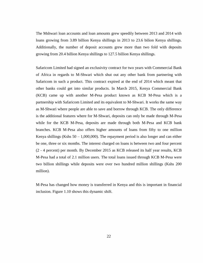
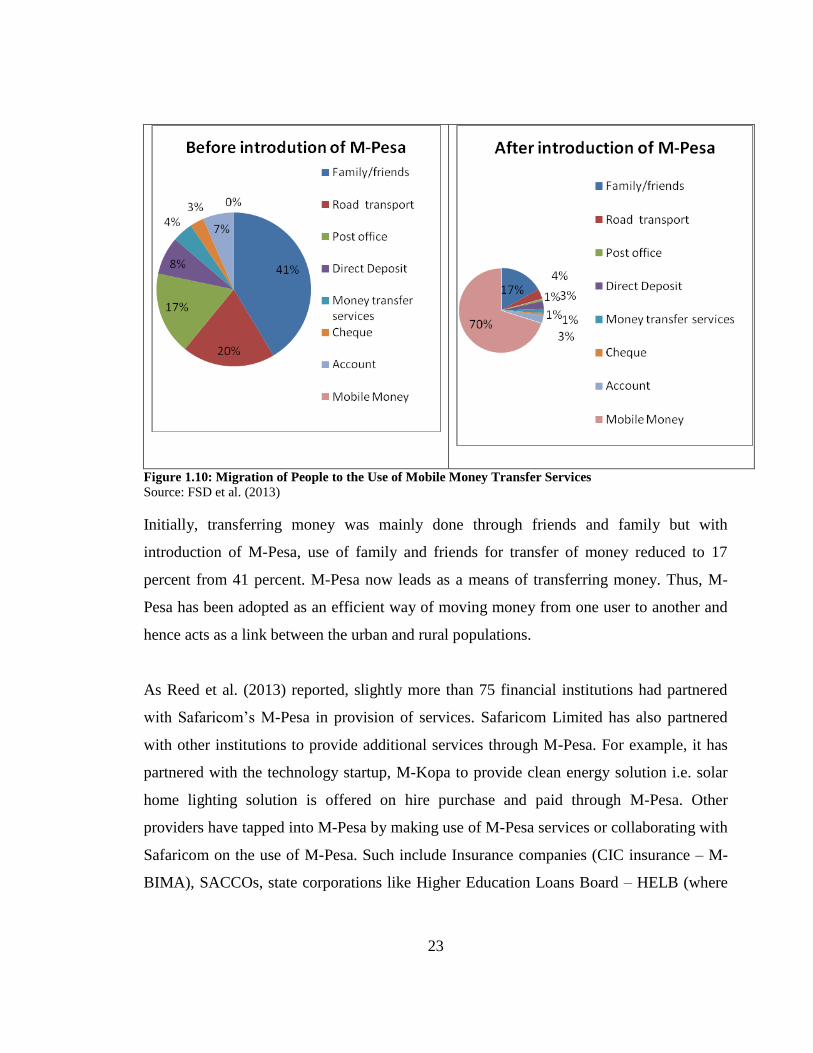
Figure 1.10: Migration of People to the Use of Mobile Money Transfer Services
Source: FSD et al. (2013)
Initially, transferring money was mainly done through friends and family but with
introduction of M-Pesa, use of family and friends for transfer of money reduced to 17
percent from 41 percent. M-Pesa now leads as a means of transferring money. Thus, M-
Pesa has been adopted as an efficient way of moving money from one user to another and
hence acts as a link between the urban and rural populations.
As Reed et al. (2013) reported, slightly more than 75 financial institutions had partnered
with Safaricom‘s M-Pesa in provision of services. Safaricom Limited has also partnered
with other institutions to provide additional services through M-Pesa. For example, it has
partnered with the technology startup, M-Kopa to provide clean energy solution i.e. solar
home lighting solution is offered on hire purchase and paid through M-Pesa. Other
providers have tapped into M-Pesa by making use of M-Pesa services or collaborating with
Safaricom on the use of M-Pesa. Such include Insurance companies (CIC insurance – M-
BIMA), SACCOs, state corporations like Higher Education Loans Board – HELB (where

24
former university students pay for their loans through M-Pesa), petrol stations and
supermarkets.
Thus, it is clear from the discussions that there are several uses of M-Pesa including
transfer and transaction, savings and credit. These four uses of M-Pesa give the key
channels through which M-Pesa trickles down to economic growth and poverty.
1.3.3 Relationship between Financial Development and Financial Innovation
Financial innovation contributes to financial development. During the period post mobile
banking introduction (after 2007), there is a connection between the financial development
indicators and the financial innovation. Using the growth of M-Pesa agents from 2007, it
was clear that the financial development indicators; credit to private sector, broad money
supply and bank deposits have all had an accelerated increase post mobile banking
introduction. Further, it was observed that non-performing loans have reduced to the less
than 10 percent mark post mobile banking introduction. These relationships are shown in
Figures A.1, A.2, A.3 and A.4. Meierrieks (2014) also found that financial development
occurs simultaneously with financial innovation. This chapter thus discussed the M-Pesa
mobile money service showing its operational framework and how it theoretically relates
to economic growth and poverty.
These new financial developments in Kenya may have implications for growth and
poverty. Therefore, this thesis sought to investigate the relationships between financial
development, economic growth and poverty. This chapter laid an important basis for the
three essays in regards to understanding the major financial developments and innovations.
However, to understand these relationships empirically, there is need to examine the
behavior of economic growth and poverty.
25
1.4 Economic Growth
Kenya has had a rather poor economic performance for over two decades. After
independence, Kenya promoted rapid economic growth through public investment, support
for agricultural production and offering incentives for private industrial investment. This
saw the Gross Domestic Product (GDP) grow by an average of 6.6 percent from 1964-
1972 but from 1974, a decline started with average annual growth averaging 5.2 percent in
the period between 1972-1979, 4.0 percent over 1980-1989 and 2.4 percent over 1990-
2000 (Republic of Kenya, 2001). This poor performance was due to poor macroeconomic
policies in the 1970‘s and 1980‘s, for example price control, import substitution and
exchange rate control. In addition, the government‘s poor governance standards deterred
domestic investment.
In the early 1990‘s structural adjustment program (SAP) were introduced by the
International Monetary Fund (IMF) and World Bank. These changes did not bring so much
change in the growth rate due to poor commitment by the government to reform and high
corruption. Other shocks in the 1990s include the after effects of the 1992 general election
where too much money was printed for the elections. These shocks together with poor
monetary and fiscal policies led to very low economic performance (Amanja and
Morrissey, 2005). Poor monetary policies led to high interest rates while poor fiscal
policies led to budget deficits.
After the National Rainbow Coalition government came into power in 2002, Kenya‘s
economic performance took an upward trend and by 2007, the economic growth rate was
at 7 percent. But the post-election violence following the 2007 elections lowered the
economic performance of the economy for the subsequent years. This was due to the
negative effects on agriculture and transport sectors which adversely affected others
sectors. The average real GDP growth rate fell to a low of 3.7 percent between 2000 and
2009. It then improved in 2010 and 2011 to an average of 6.2 percent but then fell down to
between 4 – 5 percent in 2012 and 2013. In 2014, growth rate was 5.3 percent. The World
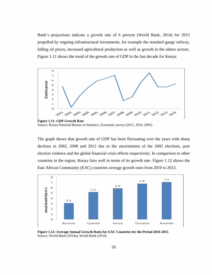
26
Bank‘s projections indicate a growth rate of 6 percent (World Bank, 2014) for 2015
propelled by ongoing infrastructural investments, for example the standard gauge railway,
falling oil prices, increased agricultural production as well as growth in the others sectors.
Figure 1.11 shows the trend of the growth rate of GDP in the last decade for Kenya.
Figure 1.11: GDP Growth Rate
Source: Kenya National Bureau of Statistics, Economic survey (2015, 2010, 2005)
The graph shows that growth rate of GDP has been fluctuating over the years with sharp
declines in 2002, 2008 and 2012 due to the uncertainties of the 2002 elections, post
election violence and the global financial crisis effects respectively. In comparison to other
countries in the region, Kenya fairs well in terms of its growth rate. Figure 1.12 shows the
East African Community (EAC) countries average growth rates from 2010 to 2013.
Figure 1.12: Average Annual Growth Rates for EAC Countries for the Period 2010-2015
Source: World Bank (2014a), World Bank (2016)

27
Looking at the averages in the last four years, the growth rate was 6.2 percent and higher
compared to Uganda‘s 5.4 percent and Burundi‘s 4.1 percent. Tanzania and Rwanda‘s
growth rate were however higher than Kenya‘s. The growth rate for Kenya is projected
upwards to 7.0 percent in 2017 (World Bank, 2014a) with the hope that there will be no
negative eventualities.
In 2014, Kenya‘s GDP was rebased and the country‘s status rose from a low income
country to a lower-middle-income country as per World Bank‘s classification. It was
necessary to rebase the GDP by using a more recent base year to collate new constant price
estimates. The old base year was 2001 while the new base year is 2009. It helps to
accommodate changes in production structures due to developments and innovations,
demand side changes like consumption patterns. Figure 1.13 shows this rebasing.
Figure 1.13: Kenya's GDP Before and After Rebasing
Source: Kenya National Bureau of Statistics (2014)
From the Figure, GDP has been on an upward trend since 2006 as most of the sectors of
the economy have been growing and their contribution increasing. By 2013, GDP stood at
US $ 55.2 Billion (Kshs. 4,757.5 Billion).
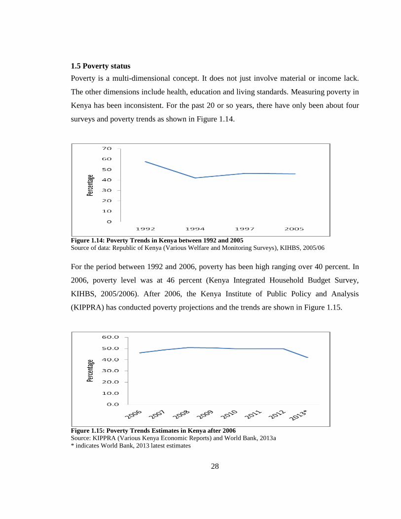
28
1.5 Poverty status
Poverty is a multi-dimensional concept. It does not just involve material or income lack.
The other dimensions include health, education and living standards. Measuring poverty in
Kenya has been inconsistent. For the past 20 or so years, there have only been about four
surveys and poverty trends as shown in Figure 1.14.
Figure 1.14: Poverty Trends in Kenya between 1992 and 2005
Source of data: Republic of Kenya (Various Welfare and Monitoring Surveys), KIHBS, 2005/06
For the period between 1992 and 2006, poverty has been high ranging over 40 percent. In
2006, poverty level was at 46 percent (Kenya Integrated Household Budget Survey,
KIHBS, 2005/2006). After 2006, the Kenya Institute of Public Policy and Analysis
(KIPPRA) has conducted poverty projections and the trends are shown in Figure 1.15.
Figure 1.15: Poverty Trends Estimates in Kenya after 2006
Source: KIPPRA (Various Kenya Economic Reports) and World Bank, 2013a
* indicates World Bank, 2013 latest estimates
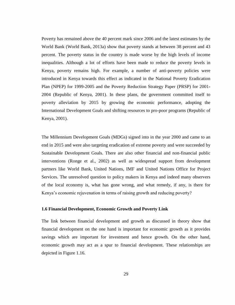
29
Poverty has remained above the 40 percent mark since 2006 and the latest estimates by the
World Bank (World Bank, 2013a) show that poverty stands at between 38 percent and 43
percent. The poverty status in the country is made worse by the high levels of income
inequalities. Although a lot of efforts have been made to reduce the poverty levels in
Kenya, poverty remains high. For example, a number of anti-poverty policies were
introduced in Kenya towards this effect as indicated in the National Poverty Eradication
Plan (NPEP) for 1999-2005 and the Poverty Reduction Strategy Paper (PRSP) for 2001-
2004 (Republic of Kenya, 2001). In these plans, the government committed itself to
poverty alleviation by 2015 by growing the economic performance, adopting the
International Development Goals and shifting resources to pro-poor programs (Republic of
Kenya, 2001).
The Millennium Development Goals (MDGs) signed into in the year 2000 and came to an
end in 2015 and were also targeting eradication of extreme poverty and were succeeded by
Sustainable Development Goals. There are also other financial and non-financial public
interventions (Ronge et al., 2002) as well as widespread support from development
partners like World Bank, United Nations, IMF and United Nations Office for Project
Services. The unresolved question to policy makers in Kenya and indeed many observers
of the local economy is, what has gone wrong, and what remedy, if any, is there for
Kenya‘s economic rejuvenation in terms of raising growth and reducing poverty?
1.6 Financial Development, Economic Growth and Poverty Link
The link between financial development and growth as discussed in theory show that
financial development on the one hand is important for economic growth as it provides
savings which are important for investment and hence growth. On the other hand,
economic growth may act as a spur to financial development. These relationships are
depicted in Figure 1.16.

30
Figure 1.16: Link between Financial Development, Economic Growth and Poverty
Source: Author‘s compilation
GROWTH
FINANCIAL
DEVELOPMENT
POVERTY
REDUCTION
A
C D
B
B
A represents the importance of financial development for growth while B represents the
importance of growth for poverty. In addition, the link between financial development and
poverty can be direct through providing self finance for the poor or indirect through
economic growth as shown by route D.
This link is important even for Kenya and it is important to understand the link especially
for policy makers. The Kenyan economy is affected by a number of dynamics both at the
macro and the micro front. Kenya aims to raise its growth rate by ensuring that the various
industries or sectors that contribute to GDP growth grow considerably. One of these
sectors is the financial sector and efforts to grow the sector are necessary. In addition, the
other main aim of every economy is to reduce poverty. This is also the World Bank‘s key
objective in addition to encouraging shared prosperity. This thesis therefore sought to
investigate how financial development in Kenya supports these key objectives of raising
growth and reducing poverty.
31
1.7 The Statement of the Problem
In Kenya, the financial sector has played a major role in mobilization of savings for growth
and development. Compared to other African countries, the Kenyan financial sector has
made significant strides (Alter and Yontcheva, 2015). The financial sector grew from 2.7
percent in 2008 to 7.5 percent in 2014 mainly due to the banking sector growth (KNBS,
2014). It contributed 6.3 percent to GDP in 2011 but fell to 4.8 percent in 2013 before
rising in 2015 to 8.4 percent (KNBS, 2015). It is evident that the financial sector has grown
speedily in the last decade. This has been accompanied by growing financial innovations.
However, economic growth has had a low fluctuating growth and poverty levels have
remained rampantly high (World Bank, 2013a). In 2007, the growth rate was 7.1 percent
reducing to 1.7 percent in 2008 after the 2007 post election violence and then increasing to
5.4 percent in 2014 (World Bank, 2014b)9. Considering the good performance of the
financial sector, the question or the problem that remains unresolved is why this good
performance has not culminated into higher economic growth and reduced poverty.
It is not clear whether financial sector development leads to economic growth in Kenya or
whether it is economic growth that leads to financial development or whether they each
spur the other. The empirical literature is divided with some studies showing the supply
leading hypothesis (Uddin et al., 2013a), others the demand following hypothesis (Ang and
Mckibbin, 2007) while others showing a bi-directional relationship (Akinlo and
Egbetunde, 2010). In Kenya, same mixed results are reached (Odhiambo, 2008;
Agbetsiafa, 2003; Wolde-Rufael, 2009 and Onuonga, 2014). Thus, there is no consensus in
Kenya on the direction of causality and how financial development impacts economic
growth. Some studies find that the impact of financial development on economic growth is
very weak in Kenya (Nyamongo, et al., 2012). Again, these studies have concentrated on
causality that other aspects of financial development have been left out. The quality and
efficiency of the financial sector development has been ignored as well as the growing
9 Latest estimates indicate a growth rate of 6 percent for 2015, World Bank (2015)
32
financial innovations and how they affect growth. This prevailing gap warrants an
empirical investigation.
Further, the debate surrounding finance and growth has ignored the finance - poverty
relationship. Poverty still remains rampant in Kenya (World Bank, 2013a) while the
financial sector is flourishing with developments and innovations (Gichuhi, 2013). The
relationship between financial development and poverty is still not clear in Kenya. The
existing studies in Kenya concentrate on micro finance and poverty (Kiiru, 2007; Okibo
and Makanga, 2014) and other aspects of financial development and poverty are left out.
The direct and indirect effects of financial development on poverty are not known. In
addition, the effect of the ongoing growth in financial innovations on poverty is
unexplored but requires immediate answers.
In the last decade, the country has experienced a number of financial innovations. The
existence of these innovations has not been looked into conclusively and thus there is a gap
in terms of understanding their theoretical implications and effect on growth and poverty.
Again, a lot of financial developments have been experienced in Kenya and even if Kenya
is relatively more advanced in financial development than other African countries (Alter
and Yontcheva, 2015), the level of financial development is still quite low compared to
other developing and developed countries. There is little literature on what drives financial
development in Kenya since much emphasis has been put on the finance-growth nexus
(Odhiambo, 2008, Wolde-Rufael, 2009 and Onuonga, 2014). Based on this background,
there is an urgent need to understand why Kenya‘s financial sector is relatively more
advanced than other African countries but trails other developing and developed countries.
Therefore, consistent with this research problem, three pressing issues should receive more
attention: What are the key drivers of financial development in Kenya?; What is the effect
of financial development on economic growth in Kenya?; and What is the effect of
financial development on poverty in Kenya?

33
1.8 Objectives of the Study
The main objective of this thesis was to investigate the relationship between financial
development, economic growth and poverty in Kenya.
Specific objectives were to:
i) Analyse the determinants of financial development in Kenya
ii) Determine the effect of financial development on economic growth
iii) Determine the effect of financial development on poverty
1.9 Significance of the Study
The findings of this study are important for policy makers in terms of making policies to
grow the financial sector, grow the economy and reduce poverty. Previous studies have not
incorporated financial innovations in the finance-growth-poverty nexus, ignoring the
qualitative and efficiency aspects of financial development, leaving out the finance-povetry
aspects and the channels of effect as well as not handling the causes of the time series
variations of financial development. These gaps are important for policy. Understanding
the key drivers for financial development are is important for policy in deciding where to
put focus. Policy makers and other stakeholders would also wish to understand what to
target in promoting financial innovations while at the same time ensuring a conducive
environment for growth. Knowing that the quality and efficiency of financial sector growth
is important is key for policy makers as they would then work on improving these aspects.
The study is useful to the regulatory authorities in the financial sector. Existing literature is
limited to traditional measurement of financial development and this study contributes
greatly to incorporating new aspects of financial development as well as financial
innovations.
34
1.10 Scope of the Study
This study examines the dynamics between financial development, growth and poverty
over time. It uses quarterly data for the period 2000 to 2014. The study is limited to Kenya
to give a better understanding of the relationship since cross country studies do not allow
one to examine the relationship exhaustively in terms of time series variations.
1.11 Structure of the Thesis
This thesis is structured into five chapters. Chapter one discusses the introduction and
financial developments and innovations that have taken place in Kenya in the last decade.
The determinants of finanacial development are discussed in chapter two. Chapter three
discusses the effect of financial development on economic growth in Kenya, while Chapter
four discusses the effects of financial developments on poverty in Kenya. Chapter five
details the summary, conclusions and policy implications.
35
CHAPTER TWO
DETERMINANTS OF FINANCIAL DEVELOPMENT
2.1 Introduction
Kenya has experienced a steady growth in the financial sector. The banking sector, the
stock and equity markets, the insurance industry and the non-bank financial institutions
have all registered impressive development patterns. These developments have been
accompanied by financial innovations such as mobile money, agency banking and ATS.
Availability and accessibility of capital promotes innovative initiatives. This is through
channeling funds from surplus to deficit investors. Financial development also enhances
the efficiency and effectiveness of institutions which promote economic growth and
poverty reduction.
Different countries experience different levels of financial development. More developed
economies experience higher financial development while less developed countries
experience lower financial development (Law and Habibullah, 2009). In as much as
developed countries experience higher financial development than less developed
countries, there are no specific thresholds to distinguish between countries that are more
financially developed from those that are not. The only thresholds that exist for developed
countries is the level of financial development that is impactful for an economy (Kose et
al., 2009). African countries‘ level of financial development has been disappointing and on
average lower than other low income countries (Alter and Yontcheva, 2015 and Easterly
and Levine, 1997). Compared to other economies in the region, Kenya seems to have a
better performance (Alter and Yontcheva, 2015) but still cannot compare to developed or
other emerging economies. Further, Kenya has made a lot of progress in terms of financial
innovation where it leads in mobile banking through M-Pesa (Allen et al., 2014). But why
are some countries more financially developed than others?

36
Kenya has experienced growth in financial development in the last decade and a half. This
could be attributed to several factors which are examined in the chapter. Figure 2.1
indicates this growth.
Figure 2.1: Trends in Financial Development Indicators
The indicators of financial development showed that financial development has been
improving with credit to private sector (CPS) and market capitalization (MKT) having an
upward trend and non-performing loans (NPL) having a downward trend. This chapter
sought to uncover the factors responsible for this time series variation in financial
development.
There are four hypotheses discussed in the literature in regards with what casues financial
development which include: The economic institutions hypothesis put forward by
Acemoglu et al. (2004), the endowment hypothesis introduced by Acemoglu et al. (2001)
both explaining the importance of institutional quality, the simultaneous openness
hypothesis due to Rajan and Zingales (2003) on the importance of openness and the law
and finance hypothesis advanced by La Porta et al. (1997) which discusses the importance
of the English common law (These are discussed in details in theoretical literature section).
Existing literature has documented several drivers of financial development. Economic
institutions enhance better environment for investment, political institutions ensure proper
37
enforcement of property rights, openness allows more opportunities for investment and
thus growth while institutional quality also enhances proper enforcement of property rights
for long-term growth. There are many studies done on what drives financial development
(See for example Huang, 2010a; Standley, 2010; Mbulawa, 2015). These studies
summarized determinants of financial development as legal tradition, institutional quality,
macroeconomic factors, openness policies, political economy factors and also other factors
as remittances, geographical factors, culture, and technology.
Most studies on determinants of financial development have concentrated on the developed
economies. Thus, less developed economies are left out in determining what causes
financial development. In Kenya, very scant evidence (Aduda et al., 2012 and Githaiga and
Kabiru, 2014) exists in this area. These few studies concluded that remittances, GDP,
inflation and domestic savings are significant determinants of financial development.
These findings were reached while looking at stock market development. These studies did
not consider significant determinants of financial development including institutional
quality, political economy factors as well as technology which has been key for financial
innovation. Thus a gap exists in understanding why the financial sector has not grown
relative to the developed economies and what determines this financial development.
Thus, this study sought answers to the following questions: What is the influence of
institutional quality, openness, macroeconomic factors and political economy on financial
development in Kenya? What are the other significant factors that influence financial
development in Kenya? The main objective of this study was to analyze the determinants
of financial development in Kenya.
Specifically, the study sought:
i) To determine the effect of institutional quality on the level of financial
development

38
ii) To determine the effect of openness indicators on the level of financial
development
iii) To determine the effect of political economy factors on the level of financial
development
iv) To determine the effect of macro economic factors on the level of financial
development
v) To determine the effect of state of technology on the level of financial development
2.1.1 Significance of the Study
This study makes contributions to an emerging literature on financial development in three
ways. First it is timely in view of the current emphasis on the role of financial development
to economic growth. Second, the study is important in terms of providing feedback to
policy makers on policies that can enhance financial development. Several factors have
been discussed in literature including institutional factors, macroeconomic factors, political
economy factors, openness factors and technology. Understanding the significant
determinants of financial development in Kenya will help policy makers to make policy
based on evidence. For example, any investigation evaluation that does not take into
account the role of financial innovation, if it is found to robustly and non-negligibly predict
financial development is therefore incomplete.
Thirdly, the study contributes to existing and new literature by bringing in new insights on
financial development in Kenya by investigating the drivers of financial development.It
does this by using appropriate indicators of financial development as opposed to the
mainly used indictors (broad money supply and domestic credit) which mainly represent
the size and depth of the financial sector and best used in developed countries. This study
thus uses bank credit to private sector to show depth of financial intermediation and
extends the analysis by including indicators of efficiency of the financial sector which
constitutes financial development. It hence contributes new knowledge in literature for not
just Kenyan policy makers but also for Kenyan and other future researchers. It fills the gap
which is missing in Kenya on what leads to financial development.
39
2.2 Literature Review
2.2.1 Theoretical Literature
Theoretical literature on the determinants of financial development centers on four
hypotheses which include the economic institutions, the endowment, the law and finance
and the simultaneous openness hypotheses. The law and finance hypothesis argued that the
English common law systems are better than the French law systems since they put
emphasis on protecting property rights (La Porte et al., 1997). The endowment hypothesis
(Acemoglu et al., 2001) argued that institutional quality is vital for development and
differs between economies due to initial differences between economies. The economic
institutions hypothesis was coined by Acemoglu et al. (2001) and proposed that good
economic institutions aid in increasing investment fueled by a good political economy.
Finally, the simultaneous openness hypothesis postulated that both trade and financial
openness promote financial development (Rajan and Zingales, 2003). These hypotheses
form an integral part of this study as it is the basis of the study. They were discussed
further in the following section.
a) Institutional Factors
Acemoglu et al. (2001) discussed the important role institutions play in economic matters
by introducing the endowment hypothesis. Institutional framework and quality differs
among regions due to initial conditions. Further, Acemoglu et al. (2004) argued that
economic institutions have an influence on the reward system facing economic actors
which is important for derivation of economic outcomes which they refer to as the
economic institutions hypothesis. Economic institutions contribute to productive and
investment decisions. This hypothesis is limited to the importance of economic institutions
while other institutions are important. Political institutions also affect the allocation and
control of power in society which determines to a greater extent, economic outcomes. In a
centralized form of government with little competition, financial systems are poorly
developed in contrast to more decentralized competitive economies (Beck et al., 2001).

40
This is because it is possible to promote the interests of the elite leading to directed credit
allocations. There are three types of institutions (Fernandez and Tamayo, 2015): legal
institutions, macroeconomic institutions and informal institutions. Legal institutions
provide the legal framework which is important in lowering the consequences of
information asymmetry which causes failure of financial institutions. Correct enforcement
of contracts and property rights is important in the financial sector where there are many
financial contracts. There is also need for a strong judicial system to improve the legal
processes.
In regards to the legal institutions, La Porta et al. (1997) introduced the law and finance
hypothesis which asserts that the English common law systems are better than the French
law systems since they put emphasis on protecting property rights. Legal institutions
impact on financial development through two channels; the political channel and the legal
adaptability channel (Beck et al., 2001). The political channel accentuates that financial
development is determined by how property rights and investors in a country are protected.
The legal adaptability channel points out the capacity of legal institutions to adapt to
changes in financial institutions and the commercial environment. The macroeconomic
institutions need to provide a good macroeconomic environment in terms of monetary,
fiscal and financial policies which boosts financial development. Finally, the informal
institutions are important in influencing people‘s trust and their attitudes in investment.
They determine how people view risk and interest. This influences their involvement in the
financial sector in terms of taking up new instruments and investing in financial markets
(Fernandez and Tamayo, 2015).
b) Openness Factors
Trade and financial openness are seen to encourage competition and thus spur the
development of financial systems (Rajan and Zingales, 2003) in what is known as the
simultaneous openness hypothesis. Opening up of markets to foreign trade may be
accompanied by opportunities for growth. It increases trade volumes which improves
41
financial deepening and hence economic growth. This increases savings and favors
financial development. Ginebri et al. (2001) argued that an increased flow in trade can lead
to growth of the financial sector. This could occur through attaining of more efficient
technology, growth of capital markets making them more active and also higher growth
both in the real economy and in the financial sector. The other probable scenario is that it
can bring foreign competition to the domestic markets. This may lower economic profits
and hence make domestic firms more dependent on external finance. This dependence
could make domestic firms push for lowered interest rate (financial repression) which is
not conducive for financial development. This hypothesis is critical in Kenya with the
country having opened up its markets to the rest of the world with various bilateral and
multilateral agreements like the East Africa Community and Common Market for Eastern
and Southern Africa.
c) Macroeconomic Factors
The theory behind the relationship between financial development and economic growth is
traced back to Schumpeter (1911) who argued that financial intermediation plays a key
role in influencing economic growth. The theory also shows a reverse causation between
financial development and economic growth where financial development follows
economic growth in what is known as demand following hypothesis or the growth led
finance. Economic growth leads to increased economic activity which calls for growth in
financial systems and thus financial development is viewed as a consequence of economic
growth (Robinson, 1952). Further, as Patrick (1966) argued, an upsurge in economic
growth leads to increased demand for financial services, financial instruments and financial
innovations. Economic growth also leads to introduction and set up of new financial
institutions and growth of existing institutions (Trew, 2006) which leads to financial
development.
Inflation is seen to negatively affect financial development. First, due to information
asymmetries, efficiency in the financial system affects how savings and investments are
allocated (Stiglitz and Weiss, 1981 and Huybens and Smith, 1999). When there is a high

42
rate of inflation, then volatility and instability in the financial markets is worsened as well
as inefficiency which creeps in the financial system thus hindering growth in the long-run.
High inflation is also seen theoretically to lead to instabilities in the financial markets
especially volatilities which are endogenously determined for example through share prices
and equity returns. Further, high inflation affects negatively the real return to savings by
eroding the value of the returns.
Secondly, the relationship between inflation and financial development may be seen from
the point of government deficit and financing (McKinnon, 1973 and Bencivenga and
Smith, 1992). Governments when faced with large budget deficits may cover it through an
inflationary tax by increasing the inflation tax base or seigniorage revenue. This may
include efforts to tax the financial system which would lead to reduction in the activities of
the financial markets and the financial system as a whole. Thirdly, inflation and financial
development are related through economic growth (Boyd et al., 1996). These theories
posited that higher economic growth is associated with lower inflation rates. Thus, because
economic growth affects both inflation rates and financial development, then it implies
higher levels of financial development. Thus, inflation and financial development are
correlated holding other things constant.
d) Political Economy Factors
Rajan and Zingales (2003) argued that the presence of political powerful elite hinders
financial development. This is because they want to keep resources to a minority elite
group, control investment capital and this leads to financial repression. In regards to
political economy Acemoglu et al. (2004) further postulated that different political
institutions and political power leads to different distribution of resources. Governments
which are more democratic have better distribution of resources than those with
authoritarian types (Siegle et al., 2004).
43
e) Remittances
The theory of how remittances and financial development are linked can be looked at from
Keynes (1936) motives of holding money; transactions, precautionary and speculative
purposes (Keynes, 1936). Households receive money for and spend it on any of the three
motives. On the precautionary and speculative motives, households direct their resources
to demand deposits, savings deposits and/or time deposits. Thus, the demand of financial
services comes in since households deposit their funds in banks for precautionary motives
and keep it in demand deposits. Other funds can be placed in time deposits as they
speculate on investment opportunities. The effect of remittances on financial development
is through two main channels; the demand side and the supply side (Demirgüç-Kunt et al.,
2010). The demand side proposes that use of formal remittance services increases financial
literacy and people are able to use formal financial services as well as extend their use in
what is referred to as ―induced financial literacy hypothesis‖. The supply side channel
argues that receipt of remittances in formal financial services increases the amount of
loanable funds which leads to credit expansion by financial institutions to private and
public sector which increases financial depth.
2.2.2 Empirical Literature
Empirical literature discusses several strands of literature including: Institutional factors,
Macro economic factors, Openness factors, Political economy factors and other factors
including remittances and technology. Macroeconomic factors include economic growth,
inflation, exchange rate, budget deficit. Economic growth promotes financial development
(demand following hypothesis). Openness factors include trade openness and financial
openness where financial openness involves opening up an economy to receive foreign
capital flows, Overseas Development Aid, foreign Direct Investment, remittances and
portfolio flows. Other factors include remittances, geography and technology. This section
discussed literature based on these five strands of financial development determinants in
literature.
44
a) Macroeconomic Factors
Macroeconomic stability is necessary for investment and hence for financial development
(Bleaney, 1996). Economic growth is seen as propelling financial development. Several
studies show that financial development is a consequence of economic growth (Shan et al.,
2001; Agbetsiafa, 2003; Waqabaca 2004; Ang and McKibbin, 2007; Odhiambo, 2007;
2009; 2010; Yu and Gan, 2010 and Esso, 2010. Literature found that those economies
which have less developed or poorly performing financial sectors are likely to experience
the demand following hypothesis where economic growth is a determinant of financial
development (Waqabaca, 2004 and Ang and McKibbin, 2007). Arestis and Demetriades
(1997), Shan et al. (2001), Agbetsiafa (2003) and Law and Habibullah (2009) found that
economic growth is positively related with banking sector and capital market development.
They argued that a higher rate of economic growth leads to more demand of financial
services which is instrumental for financial development.
Most of these studies used constant financial development indicators and found support
that economic growth is a key determinant of financial development. The most common
financial development indicators used include credit to private sector, broad money supply
and market capitalization (Arestis and Demetriades, 1997; Shan et al., 2001; Agbetsiafa,
2003; Law and Habibullah, 2009 and Yu and Gan, 2010). The same indicators have been
used in studies across Africa (Chukwu and Agu, 2009 and Esso, 2010). In Kenya, the
importance of economic growth for financial development was shown by Agbetsiafa
(2003), Odhiambo (2007; 2009 and 2010). Odhiambo (2007; 2009 and 2010) used the
same measures of financial development and found the same results. These studies also
used the same financial development indicators including broad money supply and credit
to private sector.
English (1999) using cross sectional analysis found a positive relationship between
inflation and financial development. High levels of inflation cause households to substitute
45
from financial transaction services to holding high levels of money balances which raises
the size of the financial sector. On the contrary, inflation affects financial development
negatively but with thereshhold effects. Haslog and Koo (1999) and Khan et al. (2001)
using Ordinary Least Squares (OLS) and conditional least squares respectively for cross
country analysis, found thresholds effects with Haslog and Koo (1999) finding a threshold
level of 15 percent above which inflation is hurtful to financial development and below
which there are low marginal negative effects. Khan et al. (2001) using non-linear least
squares found a threshold level of 3- 6 percent per year depending on the measure of
financial development used. Below that threshold, inflation has a positive effect on
financial development and above which, inflation is detrimental to financial development.
The reason for these conflicting results between the three studies is probably the use of
different financial development indicators. English (1999) used financial sector GDP while
Haslog and Koo (1999) uses broad money supply, deposit money bank domestic assets and
credit to private sector. Khan et al. (2001) used domestic credit to private sector and stock
market capitalization. Bank credit to private is a better measure of financial development in
developing countries (Ayadi et al., 2013) and this study adopted this measure in addition to
measures of quality of assets and stock market development.
There seem to be a consensus on a negative impact of inflation on financial development
using panel data analysis mainly GMM (Boyd et al., 2001; Naceur and Ghazouani, 2005;
Zoli, 2007; Bitten Court, 2008; Kim et al., 2010 and Al-Nasser and Jackson, 2012). Boyd
et al. (2001) for example used the Hansen (1999) methodology of threshold effects and
General Methods of Moments (GMM) and found that there is a threshold of 15 percent
above which inflation is harmful to financial sector development. Kim et al., (2010) also
found a negative relationship between inflation and financial development in the long run
using panel ARDL. However, in the short run, they found that inflation is beneficial to
financial development. They also found threshold effects of inflation.
46
Ayadi et al. (2013) using random effect panel regressions found that inflation affects
financial development negatively but the effect is most significant when there is an open
capital account. These studies mainly used the broad money supply (M2/GDP) as an
indicator of financial development which is limited in developing countries as it is
composed of currency in circulation and may not show the level of financial development.
This measure is composed of M1 and quasi-money in banks and other NBFIs. It is noted
that M1 comprises a high level of cash in circulation and other demand deposits. This
measure thus makes the definition of financial development to be limited to just the
quantity of money in circulation and in financial institutions (Ang and Mckibbin, 2007 and
Gehringer, 2013). A broader perspective of financial development to include
intermediation and quality of financial development is important. These studies apart from
Ayadi et al. (2013) ignored the importance of institutional quality for financial
development. Ayadi et al. (2013) also captured financial development in terms of meta-
efficiency (distance of a bank from a meta frontier) instead of just the size of financial
development. This study borrowed from Ayadi et al. (2013) by introducing efficiency
indicators of financial development and institutional quality variable.
Country specific studies also found that inflation is negatively related with financial
development (Lee and Wong, 2005; Keho, 2009; Ozturk and Karagoz, 2012 and Akosah,
2014). They concluded that poor macroeconomic policies are deleterious to financial
development. There is an inflationary threshold above which inflation is disastrous to
financial development and below which it has no or minimal effects (Lee and Wong, 2005,
using the threshold autoregressive method). Akosah, 2014 using Vector Error Correction
Model further showed that the negative relationship and causality between inflation and
financial development depends on the measure of financial development used. These
studies could have similar findings due to the use of similar financial development
indicators, M2. Akosah (2014) in Ghana used M2/GDP which is not an appropriate
measure in developing countries (Ang and Mckibbin, 2007). This study thus deviated by
not using this measure.

47
b) Openness Factors
Trade openness is important for financial development in developed and developing
countries (Levchenko and Quy-Toan, 2004; Huang and Temple, 2005; Herger et al., 2007).
Trade openness promotes financial development only in rich developed countries and not
in poor economies since trade openness can lead to importation of financial goods for the
poor economies. This was supported by Levchenko and Quy-Toan (2004) who observed
that openness to trade can lead economies to dwindle their financial systems if they depend
on importation of financial services and financially dependent goods and services. Using
OLS and instrumental variable analysis, they also found that trade openness is more
effective in promoting banking sector development more than equity based development.
Huang and Temple (2005) using OLS and GMM also found that in more developed
countries, trade openness is accompanied by faster financial development while in poor
less developed countries, trade openness leads to sluggish financial development. The
studies used different indicators of financial development in determining if trade openness
lead to financial development. These indicators (Credit to private sector, M2 and market
capitalization) measured only the size of financial development which limits financial
development. Only Huang and temple (2005) included a measure of quality of assets and
efficiency and this study will follow by including an indicator of quality of assets.
Cross sectional analysis when used showed that trade openness is key for financial
development (Rajan and Zingales, 2003; Klein and Olivei, 2008; Grima and Shortland,
2008; and Law, 2009). Rajan and Zingales (2003) for example employed the instrumental
variable analysis and found that trade openness positively affects financial development
which happens only if the effect is jointly with the presence of free flow of capital. Free
trade alone is not sufficient to promote financial development. Further, Grima and
Shortland (2008) using OLS, outlier robust regression and GMM found that openness to
trade is more important and leads to faster growth in the banking sector whereas it
negatively affect stock market development.

48
Panel data analysis also found that trade openness is important for financial development
(Chinn and Ito, 2002; Huang, 2005a and Voghouei et al., 2010). They all found a positive
relationship between trade openness and financial development. Using GMM panel data
analysis, Chinn and Ito (2002) however observed that trade openness in less developed
countries negatively affects equity markets development while leading to an expeditious
development in the equity markets in developed and emerging economies. They also found
that there is threshold level of institutional development that is necessary for trade
openness to promote financial development. These studies concentrated on stock market
financial development and did not show the time variant reasons of financial development.
Hence, this study looked at time series dynamics.
Financial openness is important for financial development (Klein and Olivei, 1999;
Aizenman, 2004; and Baltagi et al., 2009, Matadeen and Seetanah, 2013). Using time
series Vector Error Correction Models (VECM), they found that there is a long run effect
of financial openness on financial development. Some studies found that financial
openness positively affects financial development if there is an aspect of trade openness in
an economy (Rajan and Zingales, 2003; Aizenman and Noy, 2004 and Chinn and Ito,
2006). Rajan and Zingales (2003) observed that both financial openness and trade
concurrently promote financial development. Others found that financial openness can
only promote financial development if there is the presence of well functioning legal,
economic and political institutions. These studies are panel cross country analysis and it is
important to have country specific studies. Thus, this study looked at the importance of
openness for financial development in Kenya.
Financial openness is important for equity markets and the stock market. Demetriades and
Andrianova (2005), Chinn and Ito (2006) and Demetriades and Law (2006) using GMM
and panel ECM models found that financial openness (capital account openness) leads to
financial development in the stock market and equity market in emerging economies as
well as in less developed economies but not in developed economies. Financial openness
49
is also very important for banking sector development (Law, 2008; Klein and Olivei, 2008;
Erosy, 2011 and Abzari et al., 2011). Klein and Olivei (2008) found a positive relationship
between financial openness and financial development only in the presence of institutional
quality and sound macroeconomic policies while Erosy (2011) using ARDL cointegration
approach found a relationship to exist only in the long run. Unexpectedly, financial
openness is seen to prohibit financial development. Using dynamic panel data analysis,
Voghouei et al. (2010) found that financial openness negatively affects banking sector
development. These studies used broad money as the indicator of financial development
which may not be a good indicator in developing countries. Hence, this study used other
appropriate indicators of financial development.
c) Institutional Factors
Institutional quality and institutional factors like legal laws, governance and corruption are
found to be important for financial development (La Porta et al., 1997; Levine, 1998; Law
and Demetriades, 2006; Law and Habibullah, 2009; Assane and Malamud, 2010 and
Becerra et al., 2012). Good legal laws and rules which protect investors, creditor rights and
enforcement rights have a positive impact on the size and growth of equity, stock and debt
markets as well as banking sectors in overall financial development (La Porta et al., 1997;
Levine, 1998).
The English legal origin has been found to lead to more financial development than the
French civil law because the French legal origin is associated with poor investor protection
(La Porta et al., 1997). In addition to legal rights to creditors, better information sharing
institutions leads to higher financial development in both the banking and the stock
markets (Djankov et al., 2007). Assane and Malamud (2010) further supported that the
English legal origin is superior to the French legal origin since it protects property rights
more.
50
Institutional quality leads to improvement in financial development only in the long run
(Huang, 2010b). Using General Method of Moments (GMM) in transition and low income
countries, Huang found that institutional quality is important for financial development in
poor countries in the long run. However, Sharma and Nguyen (2010) using OLS and a
financial development index made of banking development indicators observed that while
law enforcement and overall institutional quality is important for financial development,
the importance is too over emphasized in literature. They indicate that the banking sector
in Fiji developed quickly even in the absence of good institutions. Becerra et al. (2012)
developed an index of institutional quality composed of corruption, law and order and
bureaucratic quality and using GMM and Instrumental Variable (IV) methodology found
that better institutional quality leads to better financial development.
Several factors have a significant and positive effect on financial development in the
conditions of a good legal and institutional framework. These factors include trade
openness, financial openness (Beji, 2007). Their effect on financial development can only
be felt when a certain threshold of institutional quality is maintained. This literature wass
limited to cross country analysis using GMM panel and OLS analysis leaving out time
variant analysis on specific countries. This study looked at a Kenyan study and includes
institutional quality variables which have been left out in the Kenyan literature. The study
also used different financial development indicators.
d) Political Economy Factors
Political power is key in the performance of the financial sector (Beck et al., 2001). They
used panel estimation and found that political economies with open, competition and
democratic status have better performing financial sectors than the authoritarian and closed
political economies with centralized power. Electoral democracy is also seen to be a
significant determinant of financial development. It leads to better financial development
as it reduces the interest of governments to have public ownership of commercial banks.
51
When privatization is encouraged, it leads to increased competition and better performance
of the financial sector (La Porta et al., 2002). Siegle et al. (2004) using GMM estimation
found that electoral democracy and political freedom leads to higher financial development
since electoral democracy comes with stronger institutions; legal, rule based and hence
property rights protection. Stable political systems and regimes with minimal political
constraints on the leaders increase financial deepening (Huang, 2005b). Further, Grima
and Shortland (2008) used OLS and GMM models and found that major changes in
political regimes have negative effects on financial development. It was important to
borrow from these studies and test whether political economy variables affect financial
development in Kenya especially with the improvement in democratic accountability
index.
Voghouei at al. (2011b) used several political economy indicators including executive
recruitment, political competition, political checks and balances, executive constraints and
freedom of press in a GMM estimation. They found that political power is a significant
influencing factor to economic institutions which then is key for financial development.
They argued that whether political power is practiced in either an authoritarian or
democratic way influences the performance of the financial sector.
e) Remittances
In regards to remittances, a negative relationship has been found between remittances and
financial development (Adams and Page, 2005; Brown et al., 2011 and Githaiga and
Kabiru, 2014). Adams and Page (2005) for example showed that remittances are mainly
transferred through informal means instead of the formal bank and other financial
channels. This does not lead to financial development since it does not grow the formal
financial sector. Githaiga and Kabiru (2014) used a panel of 31 countries, Kenya included
and GMM estimation to show the importance of remittances and found a negative
relationship. Others, through cross country analysis show that remittances are important
52
and positively related to financial development (Aggarwal et al., 2011; Chowdhury, 2011;
Oke et al., 2011 and Gwama, 2014).
There is the demand side channel of the effect of remittances on financial development and
the supply side channel. On the demand side, Orozco and Fedewa (2005) found that receipt
of remittances induces the recipients to demand more financial services in banks, for
example bank accounts. Aggarwal et al. (2006) and Demirgüç-Kunt et al. (2010) using
GMM estimation posited that receipt of remittances through remittance transfer services
allows banks to find the unbanked receipts to offer them financial services which increase
the population with access to financial services. The high costs of sending remittances may
encourage recipients to demand certain financial products to reduce this cost. Oke et al.
(2011) using OLS and GMM in Nigeria found that remittances have no effect on credit to
private sector but has a significant effect of broad money supply indicating that most of the
remittances are used for consumption and not investment.
On the supply side, remittances are associated with an increase in financial depth due to
increase in credit of availability. Demirgüç-Kunt et al. (2010) using panel data for Mexico
showed that remittances lead to improved credit and hence financial depth. Financial
institutions are also more likely to offer credit facilities to remittance recipients since they
can afford to repay as remittances are seen as a stable income (Aggarwal et al., 2010).
These remittances also increase the level of deposits and hence the amount of loanable
funds which then increases the depth of the financial sector. However, Brown et al. (2011)
and Githaiga and Kabiru (2014) refuted the supply side channel by finding that remittances
are negatively related with credit to private sector and Foreign Direct Investment and
hence remittances hinder financial deepening. This is because receipt of remittances
curtails the use of formal banking. This shows that the use of financial development
indicators give differing results which could be due to the fact some indicators like money
supply is an unsuitable indicator in developing countries (Ang and Mckibbin, 2007). This
study introduced new indicators of financial development like non-performing loans. It
53
also considered the effect of remittances on financial development on a country specific
study instead of the cross country analysis.
f) Technology
Berger (2003) and Beccalli (2007) using OLS and 2SLS found that technology use is high
in the banking sector. Use of technology has led to reduction in costs, improvement in
financial services offered as well as increases in productivity of the banks. This is one way
of increasing financial development. Hauswald and Marquez (2003) found that information
technology leads to reduced information asymmetry which lowers the cost of borrowing
due to improved information processing. This leads to better performance of not only the
credit markets but also insurance and securities markets. Industries with use of better
technology are able to access more external finance and the financial sector is able to
provide financial services when technology use is higher (Iliya and Samaniego, 2011 using
fixed effects for a panel of countries).
Technology is a significant determinant of financial development (Marinc, 2013). Marinc
discussed that use of Information Technology (IT) helps banks to tailor their services to the
needs of customers and thus strengthens the relationship of the bank and its customers.
Such banks are able to exploit economies of scale using technology and financial
innovation which is an example of growth in the use of IT and thus improve their
marketability. The use of mobile technology has led to increased financial development.
Dekle and Pundit (2015) using panel data random effects and a financial development
index for 23 Asian countries found that increased mobile subscription has led to higher
financial development.
Literature on technology effect on financial development is growing and there are no
specific studies in Kenya on it. This is necessary especially with the growth in innovations
emanating from mobile technology. The study also deviated from use of standard financial

54
development indicators like broad money supply and domestic credit which mainly show
the size and depth of financial development.
g) Geography
Geographical factors play a significant role in promoting or hindering financial
development (Huang, 2005a; Herger et al., 2007). Whether a country is landlocked or not
and is of specific latitude area has a direct effect on financial development. The effects of
geography are felt on one side, either the supply side or the demand side like in import
demands (Herger et al., 2007). However, geography is mainly used for cross country or
cross sectional studies and may not help to account for time variant changes in financial
development.
2.2.3 Overview of the Literature
The literature summarized two main strands; the indicators of financial development and
the key drivers of financial development. With regard to financial development, several
indicators have been used including broad money supply (M2/M3), domestic credit to
private sector, and growth of liquid liabilities (Akosah, 2013; Ayadi et al., 2013). These
with the exemption of domestic credit to private sector are indicative of the size of the
financial sector and may not be appropriate for use in less developed and developing
economies (Ang and Mckibbin, 2007 and Gehringer, 2013) as they do not indicate the
ability of the financial system to convert savings to investment. They thus limit the
definition of financial development to just quantity of money available. Financial
development ought to include the aspect of intermediation, how savings are converted into
investment as well as the quality and efficiency aspects of it. Indicators like the ones used
in this study including credit to private sector, non-performing loans and interest rate
spread cover these aspects of financial development.
55
Other indicators include, credit to private sector, equity market liquidity, rate of return and
bond market capitalization (Boyd et al., 2001; Ozturk and Karagoz, 2012). Studies done in
Kenya (Aduda et al., 2012 and Standley, 2010) have used the same measures on stock
market development and banking sector development. The use of these indicators is
limited and leaves out crucial aspects of quality and efficiency. Thus, this study introduced
non-performing loans to capture quality of financial development in addition to credit to
private sector and market capitalization.
Main drivers of financial development in literature include: openness, macroeconomic
variables, institutional variables, political economy factors and remittances. Studies done
in Kenya concentrate on stock market (Aduda et al., 2012) while others are cross country
studies (Standley, 2010). They also leave out crucial drivers like institutional quality and
mobile technology which has led to the leading innovations in Kenya (M-Pesa mobile
money) and thus a critical determinant. This study filled these gaps.
2.3 Methodology
2.3.1 Theoretical Framework
The theoretical framework of the determinants of financial development can be modeled
from the three hypotheses explaining the theory of financial development as discussed in
section 2.2.1. The first one is the endowment hypothesis which stresses the importance of
institutional quality for financial development. Next is the economic institutions hypothesis
which explains that economic institutions are key for financial development (Acemoglu et
al., 2004). Additionally, the simultaneous openness hypothesis due to Rajan and Zingales
(2003) discusses that openness, both financial and trade is beneficial for local investors and
hence important for financial development. This happens through the ability to access
finance for investment. The endowment and economic institutions hypotheses are related
as they lay the importance of institutions and institutional quality. Thus, the financial
development model is represented as:
56
),,( POLITICOPENNSINSTITUTIOfFD .……………………………………………2.1
Where FD is financial development, INSTITUTIONS represent a combination of
endowment and economic institutions hypotheses while OPEN represent openness as per
the simultaneous openness hypothesis10
. The economic institutions hypothesis also argues
that for economic institutions to promote development then there should be a stimulating
political economy. Thus, POLITIC represents political economy factors. The theoretical
literature also proposes several other determinants of financial development including
macro economic variables such as inflation (Bleaney, 1996 and Hybens and Smith, 1999),
GDP which is seen to influence demand for financial services in what is known as the
demand following hypothesis (Robinson, 1952; Patrick, 1966). There are also other
determinants which influence financial development like remittances (Demirgüç-Kunt et
al., 2010), culture (Stulz and Williamson, 2003) and geography (Kamarck, 1976;
Acemoglu et al., 2001). Further, King and Levine (1993b) shows that finance responds to
other interventions and innovations through technology. Therefore, equation 2.1 is
augmented with additional factors and shown as:
),,,,( OTHERMACROPOLITICOPENNSINSTITUTIOfFD …………..…………….2.2
Where MACRO is macro economic variables while OTHER is other important factors that
affect financial development like remittances, culture, geography and technology.
2.3.2 Model Specification
The determinants of financial development are taken from the hypotheses on the
determinants of financial development and empirical literature and include institutional
factors, openness variables, political economy variables and other variables (macro
10
The law and finance hypothesis was not included since it focuses on factors that are historical in nature and
which do not vary with time and are best in explaining cross country determinants of financial development.
57
economic variables, and other factors like technology and remittances11
) as indicated in
equation 2.2. From equation 2.2, the specific indicators are introduced and following
Huang (2005a) and Seetanah et al. (2010), the specification is given as:
),,,,,,( TEREMGDPDMTOINSTfFD ……………………………..………………2.3
Where INST is the institutional quality index representing endowment and economic
institutions hypotheses, TO is trade openness representing openness hypothesis. The study
used trade openness to represent the openness hypothesis due to data limitation on
financial openness. GDP and are GDP per capita and inflation respectively and represent
macro economic variables. DM is democratic accountability and represent political
economy factors while REM and TE are remittances and mobile technology respectively.
The institutional quality index measuring economic institutions is a summation of five
indicators including; corruption, bureaucratic quality, rule of law, government repudiation
of contracts and risk of expropriation. Corruption is included in the institutional quality as
a measure of quality of economic institutions (Knack and Keefer, 1995 and Baltagi et al.,
2007) since high corruption is seen to erode the property rights protection including the
functioning of the legal systems which lowers financial development.
FD is the dependent variable representing financial development. A number of indicators
have been proposed in literature as measurements for financial development among them
are the key ones; money supply (M2/M3) and domestic credit. However, these two
measures have been criticized in literature as discussed in the literature review. Thus, this
study introduced other indicators of financial development to capture the size, quality and
efficiency of financial development. Bank credit to private sector is used as a measure of
financial depth to specifically show the capability of the banking sector to provide savings
11
Some variables like culture and geography have been discussed in literature as determining financial
development. These variables are used mainly for cross country or cross sectional studies and may not help
to account for time variant changes in financial development. Again, the sample size is not sufficiently large
to allow for enough degrees of freedom. Thus, the variables were dropped out of the study.
58
for investment. Market capitalization is used as a measure of the size of stock market while
non-performing loans shows the quality of credit given out by banks as well as efficiency
of the financial sector (Dudian and Popa, 2013).
Equation 2.3 can be rewritten as a dynamic log-linear model as follows:
4.2.................................................................................................lnln
lnlnlnlnlnlnln
76
54321100
ttt
ttttttt
TEREM
DMGDPTOINSTFDFD
The dependent variable is included as a lagged independent variable since previous values
of financial development can influence the current values of financial development
(Baltagi et al., 2007). It also helps to show the adjustment to long-run equilibrium of
financial development from its short run dynamics. FD is represented by credit to private
sector, market capitalization and non-performing loans implying that there are three
different models of financial development for each indicator.
aTEREM
DMGDPTOINSTCPSCPS
ttt
ttttttt
4.2................................................................................................lnln
lnlnlnlnlnlnln
76
54321100
bTEREM
DMGDPTOINSTMKTMKT
ttt
ttttttt
4.2................................................................................................lnln
lnlnlnlnlnlnln
76
54321100
cTEREM
DMGDPTOINSTNPLNPL
ttt
ttttttt
4.2.................................................................................................lnln
lnlnlnlnlnlnln
76
54321100
Equation 2.4 includes a test of the endowment and economic institutions hypotheses which
is explained by α1. If this coefficient is significant and positive, then
institutions/institutional quality is important in promoting financial development as
explained by the economic institutions and endowment hypothesis put forward by
Acemoglu et al. (2004; 2001) respectively. The openness hypothesis is explained by the
coefficient α2. This hypothesis is limited to trade openness due to unavailability of data on
financial openness. It is expected to be positive and significant for the hypothesis to hold
as explained by the openness hypothesis by Rajan and Zingales (2003).

59
α3 and α4 captures the importance of macro economy on financial development and are
expected as; α3 >0 and α4 < 0. α3 shows the demand following hypothesis by Patrick (1966)
that financial development follows economic growth. α4 shows that inflation is bad for
financial development. α5 is expected to be positive as argued by Acemoglu et al. (2004)
that it fuels good institutions investment and thus financial development. α6 and α7 are
expected to be positive and significant. α6 is expected to be positive and shows the
―induced financial literacy hypothesis‖ on the demand side and credit expansion on the
supply side (Demirguc-Kunt et al., 2010) and is expected to be positive. α7 is expected to
be positive since technology leads to reduced information asymmetry and hence higher
financial development (Hauswald and Marquez, 2003).
2.3.3 Definition and Measurement of Variables
This section presents the definition and measurement of variables which is shown in Table
2.1.

60
Table 2.1: Definition and Measurement of Variables
Variable Definition and measurement Expected
Sign
Literature Source Unit of
Measurement
Credit to Private Sector
(CPS)
Credit allocated by banks to the private sector only. It is a measure of financial depth and hence
size of financial development. It‘s one of the
indictors of FD
Dependent variable
Yartey, 2007 and Arcand et al., 2011
Kshs.
Market
Capitalization
(MKT)
Value of all outstanding shares of all companies
listed at the Nairobi Stock exchange and it shows
the size of stock market development. It‘s one of the indictors of FD
Dependent
variable
Kenourgios and Samitas,
(2007) and Levine (2003)
Kshs.
Non-
performing Loans (NPL)
Sum of loans for which the borrowers have not
made payment for atleast 90 days. It is measured as the value of NPLs divided by the total value of
the loan portfolio. It‘s one of the indictors of FD
Dependent
variable
Dudian and Popa (2013) Ratio
GDP Per Capita
(GDP)
The GDP divided by total population. It measures
the total product of a country
Positive
(demand following
hypothesis)
Khan et al. (2011), Kar et
al. (2015)
Kshs.
Inflation ( ) Continuous increment in price levels of goods and services over a certain time period. Measured
month on month then aggregated quarterly
Negative Easterly and Fischer (2001), Jeanneney and
Kpodar (2011), Dollar and
Kraay (2002)
Rate
Trade Openness (TO)
Aggregate of exports and imports of goods and services over GDP. Measures a country‘s
openness to trade
Positive Dauda and Makinde (2014), Menyah et al.
(2014) and Wolde -Rufael (2009)
Index
Institutional
Quality (INST)
It is a measure of how strong institutions are and
is the summation of three12 Political Risk
Services (PRS) indicators including; corruption, bureaucratic quality and risk of expropriation. It
is measured as an index from 0 = low
institutional quality to 6 = high institutional quality13
Positive Baltagi et al., 2007, Gries
and Mierrieksy (2010)
Index
Democratic
Accountability (DM)
How free and fair elections are as well as the
extent to which a government is responsive to its citizens (ICRG, 2015). It is measured as an index
from 0 = least democratic to 6 = most democratic
Positive Baltagi et al., 2007, Gries
and Mierrieksy (2010)
Index
Remittances
(REM)
Sum of the money sent back home from persons
in a foreign country and transfers by migrants
Positive Demirguc-Kunt et al.
(2010), Aggarwal et al. (2010)
Kshs.
Mobile Phone
Technology (TE)
Defined as use of mobile phones. Measured as
the number of mobile phones owned by people
Positive Marinc (2013), Aker and
Mbiti (2010)
Number
12
Baltagi et al. (2007) describes institutional quality as a summation of five PRS indicators including
corruption, bureaucratic quality, rule of law, government repudiation of contracts and risk of expropriation.
However data on rule of law and government repudiation of contracts was not available limiting us to use
only 3 PRS indicators. Corruption is measured as an index from 0 = most corrupt to 6 = least corrupt,
bureaucratic quality is also scaled from 0 = Least bureaucratic quality to 6 = best bureaucratic quality and
risk of expropriation is scaled from 0 = most risky to 10 = least risky.
13
The risk of expropriation measure which is scaled from 0 – 10 is first converted to 0 to 6 by multiplying it
by 3/5 to ensure that it is comparable to the other two indicators. The three PRS indicators are then summed
up to give the institutional quality indicator.
61
All the variables were in natural logarithm form14
. The study uses LN to represent natural
logarithm.
2.3.4 Data Type and Sources
Quarterly data on financial development indicators (credit to private sector and non-
performing loans) was obtained from the Central Bank of Kenya while market
capitalization was obtained from the Nairobi Securities Exchange. Quarterly data on
inflation, trade openness and remittances was also obtained from the Central Bank of
Kenya. Data on GDP per capita was obtained from World Development Indicators and
converted to quarterly. The data on PRS indicators including corruption, bureaucratic
quality and risk of expropriation as well as democratic accountability data was obtained
from International Country Risk Guide (ICRG) which is given on a monthly basis but
averaged to quarterly. Finally, quarterly data on the number of mobile phones to captures
technology was obtained from Communications Commission of Kenya (CCK).
2.3.5 Estimation and Testing
a) Descriptive Statistics
It was essential to conduct a descriptive statistics analysis in order to give the estimable
models the proper functional form and generate reliable estimates. The study checked for
skewness and kurtosis and used the Jarque-Bera test to check for normally properties of
variables. For a variable to be normally distributed, its skewness should be equal to zero,
kurtosis should be equal to three and the JB statistics should be equal to zero. Further, the
study sought to determine the spread of the data by estimating the mean and the standard
deviation for all the variables contained in the models. A graphical analysis of the variables
which are in logarithms was also presented to capture their movement over time.
14
While taking the natural logarithms of inflation and interest rate spread, we add one, ln(1+ ) and
ln(1+INT) INT since this gives a very close approximation (Judson and Orphanides, 1996; Ghosh and
Phillips, 1998 and Vinayagathasan, 2013)
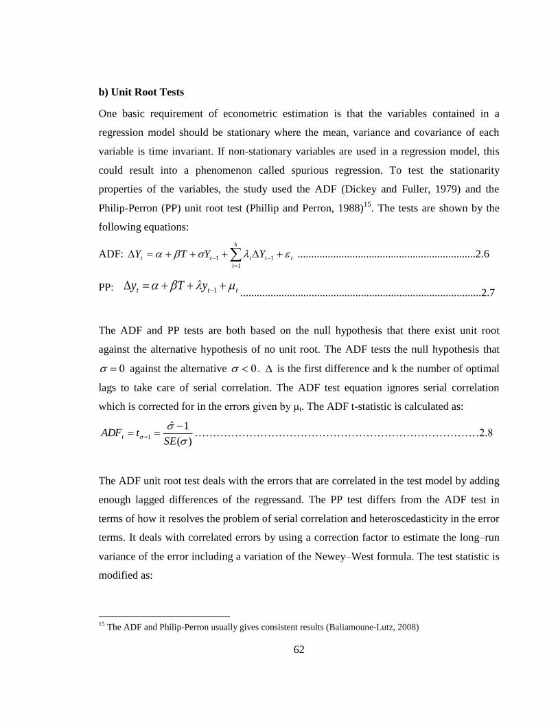
62
b) Unit Root Tests
One basic requirement of econometric estimation is that the variables contained in a
regression model should be stationary where the mean, variance and covariance of each
variable is time invariant. If non-stationary variables are used in a regression model, this
could result into a phenomenon called spurious regression. To test the stationarity
properties of the variables, the study used the ADF (Dickey and Fuller, 1979) and the
Philip-Perron (PP) unit root test (Phillip and Perron, 1988)15
. The tests are shown by the
following equations:
ADF: t
k
i
titt YYTY
1
11 .................................................................2.6
PP: ttt yTy 1 ........................................................................................2.7
The ADF and PP tests are both based on the null hypothesis that there exist unit root
against the alternative hypothesis of no unit root. The ADF tests the null hypothesis that
0 against the alternative 0 . is the first difference and k the number of optimal
lags to take care of serial correlation. The ADF test equation ignores serial correlation
which is corrected for in the errors given by μt. The ADF t-statistic is calculated as:
)(
1ˆ1
SEtADFt
……………………………………………………………………2.8
The ADF unit root test deals with the errors that are correlated in the test model by adding
enough lagged differences of the regressand. The PP test differs from the ADF test in
terms of how it resolves the problem of serial correlation and heteroscedasticity in the error
terms. It deals with correlated errors by using a correction factor to estimate the long–run
variance of the error including a variation of the Newey–West formula. The test statistic is
modified as:
15
The ADF and Philip-Perron usually gives consistent results (Baliamoune-Lutz, 2008)
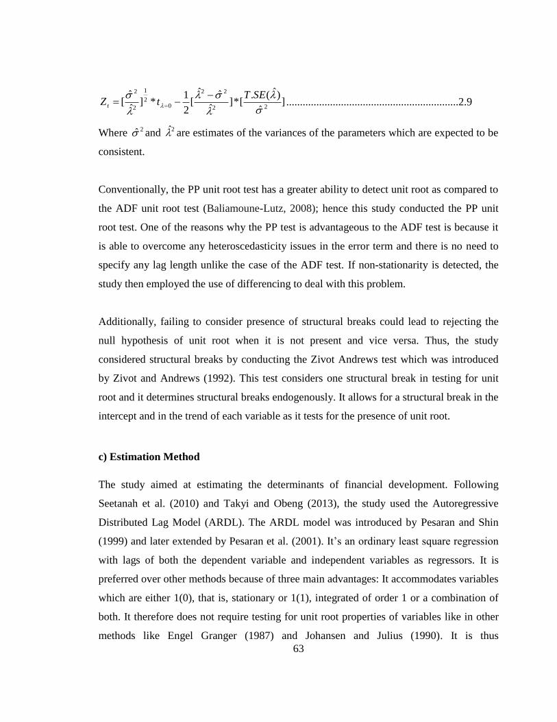
63
]ˆ
)ˆ(.[*]
ˆ
ˆˆ[
2
1*]
ˆ
ˆ[
22
22
02
1
2
2
SETtZ t
...............................................................2.9
Where 2̂ and 2̂ are estimates of the variances of the parameters which are expected to be
consistent.
Conventionally, the PP unit root test has a greater ability to detect unit root as compared to
the ADF unit root test (Baliamoune-Lutz, 2008); hence this study conducted the PP unit
root test. One of the reasons why the PP test is advantageous to the ADF test is because it
is able to overcome any heteroscedasticity issues in the error term and there is no need to
specify any lag length unlike the case of the ADF test. If non-stationarity is detected, the
study then employed the use of differencing to deal with this problem.
Additionally, failing to consider presence of structural breaks could lead to rejecting the
null hypothesis of unit root when it is not present and vice versa. Thus, the study
considered structural breaks by conducting the Zivot Andrews test which was introduced
by Zivot and Andrews (1992). This test considers one structural break in testing for unit
root and it determines structural breaks endogenously. It allows for a structural break in the
intercept and in the trend of each variable as it tests for the presence of unit root.
c) Estimation Method
The study aimed at estimating the determinants of financial development. Following
Seetanah et al. (2010) and Takyi and Obeng (2013), the study used the Autoregressive
Distributed Lag Model (ARDL). The ARDL model was introduced by Pesaran and Shin
(1999) and later extended by Pesaran et al. (2001). It‘s an ordinary least square regression
with lags of both the dependent variable and independent variables as regressors. It is
preferred over other methods because of three main advantages: It accommodates variables
which are either 1(0), that is, stationary or 1(1), integrated of order 1 or a combination of
both. It therefore does not require testing for unit root properties of variables like in other
methods like Engel Granger (1987) and Johansen and Julius (1990). It is thus
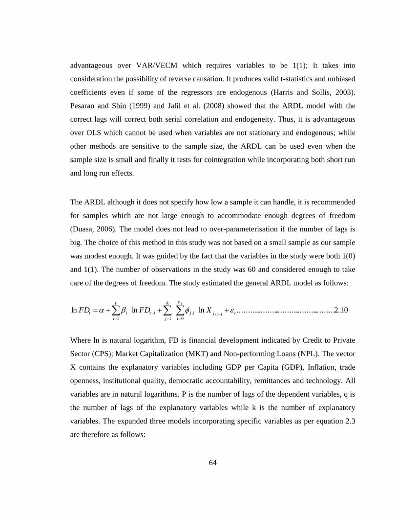
64
advantageous over VAR/VECM which requires variables to be 1(1); It takes into
consideration the possibility of reverse causation. It produces valid t-statistics and unbiased
coefficients even if some of the regressors are endogenous (Harris and Sollis, 2003).
Pesaran and Shin (1999) and Jalil et al. (2008) showed that the ARDL model with the
correct lags will correct both serial correlation and endogeneity. Thus, it is advantageous
over OLS which cannot be used when variables are not stationary and endogenous; while
other methods are sensitive to the sample size, the ARDL can be used even when the
sample size is small and finally it tests for cointegration while incorporating both short run
and long run effects.
The ARDL although it does not specify how low a sample it can handle, it is recommended
for samples which are not large enough to accommodate enough degrees of freedom
(Duasa, 2006). The model does not lead to over-parameterisation if the number of lags is
big. The choice of this method in this study was not based on a small sample as our sample
was modest enough. It was guided by the fact that the variables in the study were both 1(0)
and 1(1). The number of observations in the study was 60 and considered enough to take
care of the degrees of freedom. The study estimated the general ARDL model as follows:
10.2..................................................lnlnln ,
0
,
11
titj
n
i
ij
k
j
it
p
i
it XFDFDj
Where ln is natural logarithm, FD is financial development indicated by Credit to Private
Sector (CPS); Market Capitalization (MKT) and Non-performing Loans (NPL). The vector
X contains the explanatory variables including GDP per Capita (GDP), Inflation, trade
openness, institutional quality, democratic accountability, remittances and technology. All
variables are in natural logarithms. P is the number of lags of the dependent variables, q is
the number of lags of the explanatory variables while k is the number of explanatory
variables. The expanded three models incorporating specific variables as per equation 2.3
are therefore as follows:
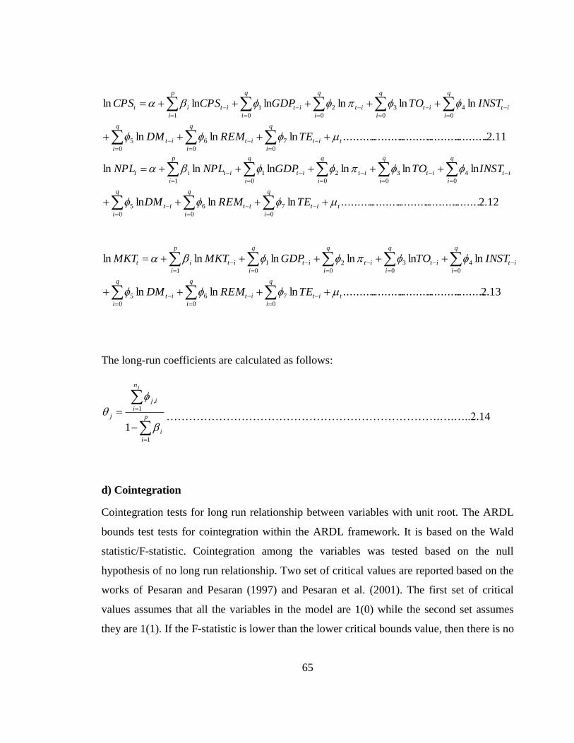
65
11.2...................................................lnlnln
lnlnlnlnlnln
0
7
0
6
0
5
0
4
0
3
0
2
0
1
1
tit
q
i
it
q
i
it
q
i
it
q
i
it
q
i
it
q
i
it
q
i
it
p
i
it
TEREMDM
INSTTOGDPCPSCPS
12.2.................................................lnlnln
lnlnlnlnlnln
0
7
0
6
0
5
0
4
0
3
0
2
0
1
1
tit
q
i
it
q
i
it
q
i
it
q
i
it
q
i
it
q
i
it
q
i
it
p
i
it
TEREMDM
INSTTOGDPNPLNPL
13.2.................................................lnlnln
lnlnlnlnlnln
0
7
0
6
0
5
0
4
0
3
0
2
0
1
1
tit
q
i
it
q
i
it
q
i
it
q
i
it
q
i
it
q
i
it
q
i
it
p
i
it
TEREMDM
INSTTOGDPMKTMKT
The long-run coefficients are calculated as follows:
p
i
i
n
i
ij
j
j
1
1
,
1
……………………………………………………………….….…..2.14
d) Cointegration
Cointegration tests for long run relationship between variables with unit root. The ARDL
bounds test tests for cointegration within the ARDL framework. It is based on the Wald
statistic/F-statistic. Cointegration among the variables was tested based on the null
hypothesis of no long run relationship. Two set of critical values are reported based on the
works of Pesaran and Pesaran (1997) and Pesaran et al. (2001). The first set of critical
values assumes that all the variables in the model are 1(0) while the second set assumes
they are 1(1). If the F-statistic is lower than the lower critical bounds value, then there is no

66
cointegration. If it is higher, then the presence of cointegration among the variables is
confirmed. Finally, if it falls into the critical bounds, then the results are inconclusive.
The bounds testing is estimated as follows:
15.2....................................................................................................................................
.lnlnlnlnln 1,
1
1,
1
0
*
,
1
1
1
*
ttj
k
j
jtitj
n
i
ij
k
j
it
p
i
it XFDXFDFDj
The test for long-run relationship is:
0
0.........21 k
Where there is cointegration, the ARDL error correction model is then estimated to give
the speed of adjustment from short run to long run equilibrium as follows:
16.2............................lnlnln 1,
1
0
*
,
1
1
*
ttitj
n
i
ij
k
it
p
i
it ECTXFDFDj
Where: *
i and *
,ij are the short-run co-efficients while is the speed of adjustment and is
expected to be negative.
j
k
j
tjtt XyECT
1
,ln ,
p
i
i
1
ˆ1
p
im
mi
1
* ̂ ,
jn
mim
mjij ,
*
,
2.4 Empirical Results and Discussion
2.4.1 Descriptive Statistics
To test for the normality properties of the variables, the study used JB test which compares
the skewness and kurtosis coefficients of the variables. For a variable to be normally
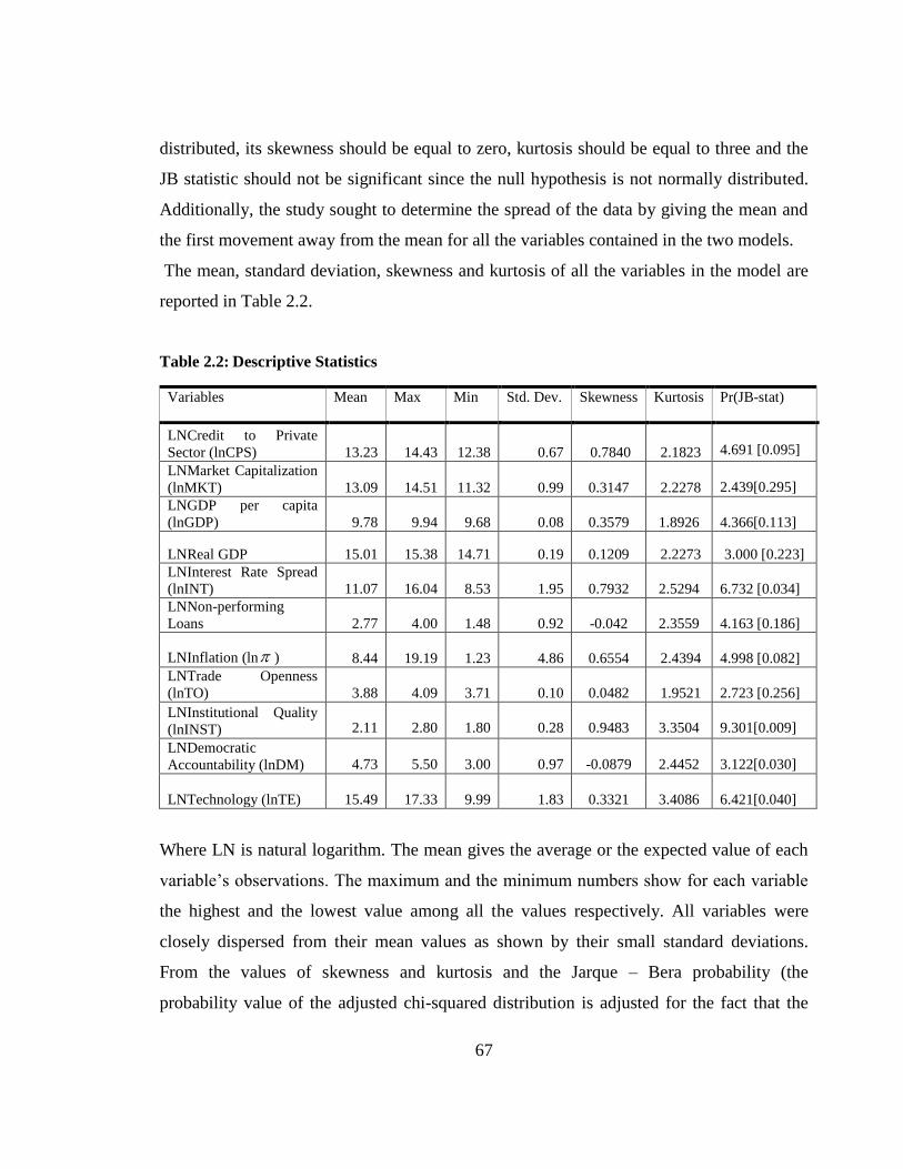
67
distributed, its skewness should be equal to zero, kurtosis should be equal to three and the
JB statistic should not be significant since the null hypothesis is not normally distributed.
Additionally, the study sought to determine the spread of the data by giving the mean and
the first movement away from the mean for all the variables contained in the two models.
The mean, standard deviation, skewness and kurtosis of all the variables in the model are
reported in Table 2.2.
Table 2.2: Descriptive Statistics
Variables Mean Max Min Std. Dev. Skewness Kurtosis Pr(JB-stat)
LNCredit to Private
Sector (lnCPS) 13.23 14.43 12.38 0.67 0.7840 2.1823
4.691 [0.095]
LNMarket Capitalization
(lnMKT) 13.09 14.51 11.32 0.99 0.3147 2.2278
2.439[0.295]
LNGDP per capita
(lnGDP) 9.78 9.94 9.68 0.08 0.3579 1.8926 4.366[0.113]
LNReal GDP 15.01 15.38 14.71 0.19 0.1209 2.2273 3.000 [0.223]
LNInterest Rate Spread
(lnINT) 11.07 16.04 8.53 1.95 0.7932 2.5294
6.732 [0.034]
LNNon-performing
Loans 2.77 4.00 1.48 0.92 -0.042 2.3559
4.163 [0.186]
LNInflation (ln ) 8.44 19.19 1.23 4.86 0.6554 2.4394
4.998 [0.082]
LNTrade Openness
(lnTO) 3.88 4.09 3.71 0.10 0.0482 1.9521
2.723 [0.256]
LNInstitutional Quality
(lnINST)
2.11
2.80
1.80
0.28
0.9483
3.3504
9.301[0.009]
LNDemocratic
Accountability (lnDM)
4.73
5.50
3.00
0.97
-0.0879
2.4452
3.122[0.030]
LNTechnology (lnTE)
15.49
17.33
9.99
1.83
0.3321
3.4086
6.421[0.040]
Where LN is natural logarithm. The mean gives the average or the expected value of each
variable‘s observations. The maximum and the minimum numbers show for each variable
the highest and the lowest value among all the values respectively. All variables were
closely dispersed from their mean values as shown by their small standard deviations.
From the values of skewness and kurtosis and the Jarque – Bera probability (the
probability value of the adjusted chi-squared distribution is adjusted for the fact that the

68
Jarque Bera test takes long to converge to a chi-squared distribution and also for small
sample sizes), GDP per capita, market capitalization, trade openness and inflation were
normally distributed at five percent significance level. At one percent significance level, all
the variables were normally distributed apart from institutional quality. These results
indicated that the data is good for the study as they help in explaining data in a simpler and
meaningful way.
2.4.2 Unit Root Test Results
Before conducting the unit root test, it was important to determine the optimal lag length of
each variable which is important when testing for unit root and when running the empirical
models. Indicating the wrong lag length could give incorrect stationarity results by
showing presence of unit root when it isn‘t there and vice versa. The tests for optimal lag
length were conducted including Fixed Prediction Error (FPE), Akaike Information
Criteria (AIC), Hannan and Quinn Information Criteria (HQIC) and Schwarz‘ Bayesian
Information Criteria (SBIC). For all the variables, all the lag length tests determined the
same lag length as shown in Table A.1 (Appendix). Credit to private sector, non-
performing loans, trade openness and remittances had a lag length of three, market
capitalization, GDP per capita, institutional quality and democratic accountability had a lag
length of one while inflation and mobile technology had a lag length of four.
The study conducted a graphical analysis of the variables (in logarithms) to capture their
movement over time. It was conducted to show whether the variables have a deterministic
trend or not. This gives guidance on whether to include a trend and intercept or not when
conducting stationarity tests. These graphs are indicated in Appendix. From the graph, it is
clear that all the variables had a trend except for institutional quality.
Unit root tests were conducted to determine the stationarity properties of the variables. One
requirement of OLS is that variables have a constant mean, variance and the covariance
between the values of two time periods is zero, failure to which can lead to spurious
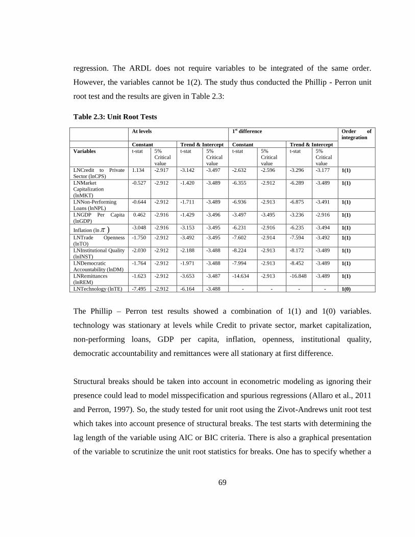
69
regression. The ARDL does not require variables to be integrated of the same order.
However, the variables cannot be 1(2). The study thus conducted the Phillip - Perron unit
root test and the results are given in Table 2.3:
Table 2.3: Unit Root Tests
At levels 1st difference Order of
integration
Constant Trend & Intercept Constant Trend & Intercept
Variables t-stat 5% Critical
value
t-stat 5% Critical
value
t-stat 5% Critical
value
t-stat 5% Critical
value
LNCredit to Private Sector (lnCPS)
1.134 -2.917 -3.142 -3.497 -2.632 -2.596 -3.296 -3.177 1(1)
LNMarket
Capitalization
(lnMKT)
-0.527 -2.912 -1.420 -3.489 -6.355 -2.912 -6.289 -3.489 1(1)
LNNon-Performing
Loans (lnNPL)
-0.644 -2.912 -1.711 -3.489 -6.936 -2.913 -6.875 -3.491 1(1)
LNGDP Per Capita
(lnGDP)
0.462 -2.916 -1.429 -3.496 -3.497 -3.495 -3.236 -2.916 1(1)
Inflation (ln ) -3.048 -2.916 -3.153 -3.495 -6.231 -2.916 -6.235 -3.494 1(1)
LNTrade Openness
(lnTO)
-1.750 -2.912 -3.492 -3.495 -7.602 -2.914 -7.594 -3.492 1(1)
LNInstitutional Quality
(lnINST)
-2.030 -2.912 -2.188 -3.488 -8.224 -2.913 -8.172 -3.489 1(1)
LNDemocratic
Accountability (lnDM)
-1.764 -2.912 -1.971 -3.488 -7.994 -2.913 -8.452 -3.489 1(1)
LNRemittances
(lnREM)
-1.623 -2.912 -3.653 -3.487 -14.634 -2.913 -16.848 -3.489 1(1)
LNTechnology (lnTE) -7.495 -2.912 -6.164 -3.488 - - - - 1(0)
The Phillip – Perron test results showed a combination of 1(1) and 1(0) variables.
technology was stationary at levels while Credit to private sector, market capitalization,
non-performing loans, GDP per capita, inflation, openness, institutional quality,
democratic accountability and remittances were all stationary at first difference.
Structural breaks should be taken into account in econometric modeling as ignoring their
presence could lead to model misspecification and spurious regressions (Allaro et al., 2011
and Perron, 1997). So, the study tested for unit root using the Zivot-Andrews unit root test
which takes into account presence of structural breaks. The test starts with determining the
lag length of the variable using AIC or BIC criteria. There is also a graphical presentation
of the variable to scrutinize the unit root statistics for breaks. One has to specify whether a
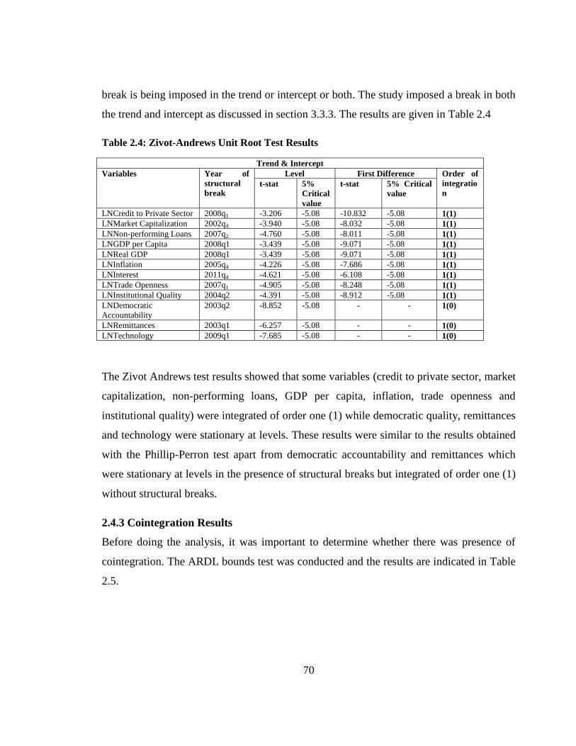
70
break is being imposed in the trend or intercept or both. The study imposed a break in both
the trend and intercept as discussed in section 3.3.3. The results are given in Table 2.4
Table 2.4: Zivot-Andrews Unit Root Test Results
Trend & Intercept
Variables Year of
structural
break
Level First Difference Order of
integratio
n t-stat 5%
Critical
value
t-stat 5% Critical
value
LNCredit to Private Sector 2008q1 -3.206 -5.08 -10.832 -5.08 1(1)
LNMarket Capitalization 2002q4 -3.940 -5.08 -8.032 -5.08 1(1)
LNNon-performing Loans 2007q2 -4.760 -5.08 -8.011 -5.08 1(1)
LNGDP per Capita 2008q1 -3.439 -5.08 -9.071 -5.08 1(1)
LNReal GDP 2008q1 -3.439 -5.08 -9.071 -5.08 1(1)
LNInflation 2005q4 -4.226 -5.08 -7.686 -5.08 1(1)
LNInterest 2011q4 -4.621 -5.08 -6.108 -5.08 1(1)
LNTrade Openness 2007q1 -4.905 -5.08 -8.248 -5.08 1(1)
LNInstitutional Quality 2004q2 -4.391 -5.08 -8.912 -5.08 1(1)
LNDemocratic
Accountability
2003q2 -8.852 -5.08 - - 1(0)
LNRemittances 2003q1 -6.257 -5.08 - - 1(0)
LNTechnology 2009q1 -7.685 -5.08 - - 1(0)
The Zivot Andrews test results showed that some variables (credit to private sector, market
capitalization, non-performing loans, GDP per capita, inflation, trade openness and
institutional quality) were integrated of order one (1) while democratic quality, remittances
and technology were stationary at levels. These results were similar to the results obtained
with the Phillip-Perron test apart from democratic accountability and remittances which
were stationary at levels in the presence of structural breaks but integrated of order one (1)
without structural breaks.
2.4.3 Cointegration Results
Before doing the analysis, it was important to determine whether there was presence of
cointegration. The ARDL bounds test was conducted and the results are indicated in Table
2.5.
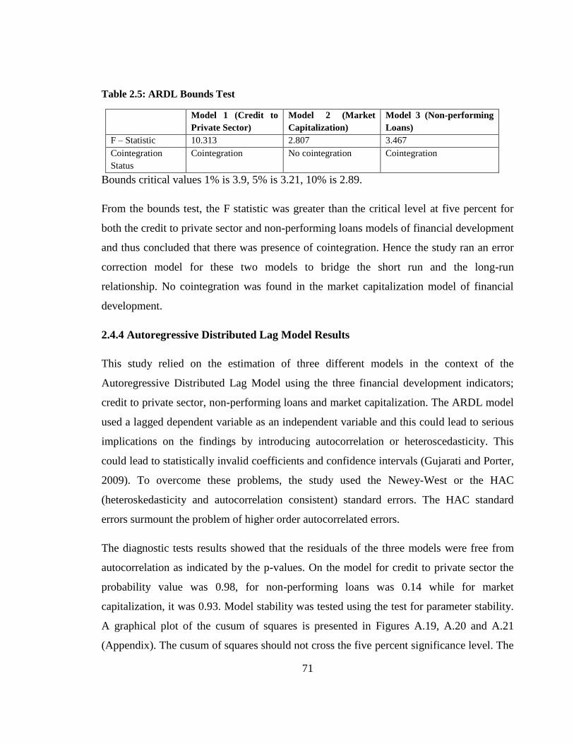
71
Table 2.5: ARDL Bounds Test
Model 1 (Credit to
Private Sector)
Model 2 (Market
Capitalization)
Model 3 (Non-performing
Loans)
F – Statistic 10.313 2.807 3.467
Cointegration
Status
Cointegration No cointegration Cointegration
Bounds critical values 1% is 3.9, 5% is 3.21, 10% is 2.89.
From the bounds test, the F statistic was greater than the critical level at five percent for
both the credit to private sector and non-performing loans models of financial development
and thus concluded that there was presence of cointegration. Hence the study ran an error
correction model for these two models to bridge the short run and the long-run
relationship. No cointegration was found in the market capitalization model of financial
development.
2.4.4 Autoregressive Distributed Lag Model Results
This study relied on the estimation of three different models in the context of the
Autoregressive Distributed Lag Model using the three financial development indicators;
credit to private sector, non-performing loans and market capitalization. The ARDL model
used a lagged dependent variable as an independent variable and this could lead to serious
implications on the findings by introducing autocorrelation or heteroscedasticity. This
could lead to statistically invalid coefficients and confidence intervals (Gujarati and Porter,
2009). To overcome these problems, the study used the Newey-West or the HAC
(heteroskedasticity and autocorrelation consistent) standard errors. The HAC standard
errors surmount the problem of higher order autocorrelated errors.
The diagnostic tests results showed that the residuals of the three models were free from
autocorrelation as indicated by the p-values. On the model for credit to private sector the
probability value was 0.98, for non-performing loans was 0.14 while for market
capitalization, it was 0.93. Model stability was tested using the test for parameter stability.
A graphical plot of the cusum of squares is presented in Figures A.19, A.20 and A.21
(Appendix). The cusum of squares should not cross the five percent significance level. The
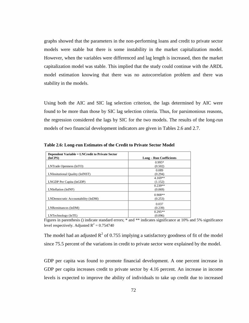
72
graphs showed that the parameters in the non-performing loans and credit to private sector
models were stable but there is some instability in the market capitalization model.
However, when the variables were differenced and lag length is increased, then the market
capitalization model was stable. This implied that the study could continue with the ARDL
model estimation knowing that there was no autocorrelation problem and there was
stability in the models.
Using both the AIC and SIC lag selection criterion, the lags determined by AIC were
found to be more than those by SIC lag selection criteria. Thus, for parsimonious reasons,
the regression considered the lags by SIC for the two models. The results of the long-run
models of two financial development indicators are given in Tables 2.6 and 2.7.
Table 2.6: Long-run Estimates of the Credit to Private Sector Model
Dependent Variable = LNCredit to Private Sector
(lnCPS) Long – Run Coefficients
LNTrade Openness (lnTO)
0.995*
(0.502)
LNInsitutional Quality (lnINST)
0.089
(0.294)
LNGDP Per Capita (lnGDP)
4.169**
(1.152)
LNInflation (lnINF)
0.239**
(0.069)
LNDemocratic Accountability (lnDM)
0.908**
(0.253)
LNRemittances (lnDM)
0.037
(0.239)
LNTechnology (lnTE)
0.295**
(0.096)
Figures in parenthesis () indicate standard errors; * and ** indicates significance at 10% and 5% significance
level respectively. Adjusted R2 = 0.754740
The model had an adjusted R2 of 0.755 implying a satisfactory goodness of fit of the model
since 75.5 percent of the variations in credit to private sector were explained by the model.
GDP per capita was found to promote financial development. A one percent increase in
GDP per capita increases credit to private sector by 4.16 percent. An increase in income
levels is expected to improve the ability of individuals to take up credit due to increased
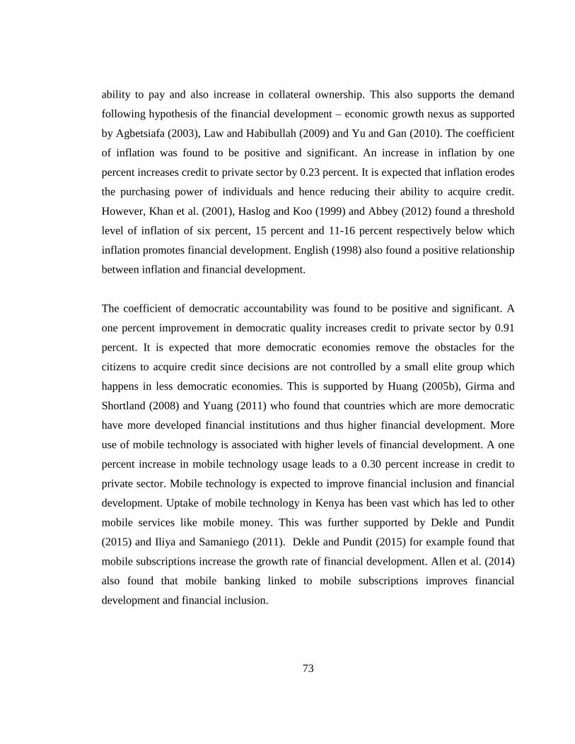
73
ability to pay and also increase in collateral ownership. This also supports the demand
following hypothesis of the financial development – economic growth nexus as supported
by Agbetsiafa (2003), Law and Habibullah (2009) and Yu and Gan (2010). The coefficient
of inflation was found to be positive and significant. An increase in inflation by one
percent increases credit to private sector by 0.23 percent. It is expected that inflation erodes
the purchasing power of individuals and hence reducing their ability to acquire credit.
However, Khan et al. (2001), Haslog and Koo (1999) and Abbey (2012) found a threshold
level of inflation of six percent, 15 percent and 11-16 percent respectively below which
inflation promotes financial development. English (1998) also found a positive relationship
between inflation and financial development.
The coefficient of democratic accountability was found to be positive and significant. A
one percent improvement in democratic quality increases credit to private sector by 0.91
percent. It is expected that more democratic economies remove the obstacles for the
citizens to acquire credit since decisions are not controlled by a small elite group which
happens in less democratic economies. This is supported by Huang (2005b), Girma and
Shortland (2008) and Yuang (2011) who found that countries which are more democratic
have more developed financial institutions and thus higher financial development. More
use of mobile technology is associated with higher levels of financial development. A one
percent increase in mobile technology usage leads to a 0.30 percent increase in credit to
private sector. Mobile technology is expected to improve financial inclusion and financial
development. Uptake of mobile technology in Kenya has been vast which has led to other
mobile services like mobile money. This was further supported by Dekle and Pundit
(2015) and Iliya and Samaniego (2011). Dekle and Pundit (2015) for example found that
mobile subscriptions increase the growth rate of financial development. Allen et al. (2014)
also found that mobile banking linked to mobile subscriptions improves financial
development and financial inclusion.
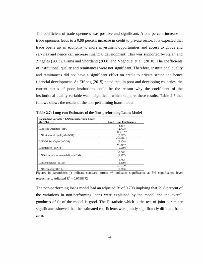
74
The coefficient of trade openness was positive and significant. A one percent increase in
trade openness leads to a 0.99 percent increase in credit to private sector. It is expected that
trade opens up an economy to more investment opportunities and access to goods and
services and hence can increase financial development. This was supported by Rajan and
Zingales (2003), Grima and Shortland (2008) and Voghouei et al. (2010). The coefficients
of institutional quality and remittances were not significant. Therefore, institutional quality
and remittances did not have a significant effect on credit to private sector and hence
financial development. As Effiong (2015) noted that, in poor and developing countries, the
current status of poor institutions could be the reason why the coefficient of the
institutional quality variable was insignificant which supports these results. Table 2.7 that
follows shows the results of the non-performing loans model.
Table 2.7: Long-run Estimates of the Non-performing Loans Model
Dependent Variable = LNNon-performing Loans
(lnNPL) Long – Run Coefficients
LNTrade Openness (lnTO)
2.814
(2.733)
LNInsitutional Quality (lnINST)
-0..216**
(0.067)
LNGDP Per Capita (lnGDP) -14.429**
(5.128)
LNInflation (lnINF)
0.145**
(0.069)
LNDemocratic Accountability (lnDM) -1.503 (1.177)
LNRemittances (lnREM)
1.782
(1.109)
LNTechnology (lnTE) -0.631** (0.313)
Figures in parenthesis () indicate standard errors; ** indicates significance at 5% significance level
respectively. Adjusted R2 = 0.0798372
The non-performing loans model had an adjusted R2
of 0.798 implying that 79.8 percent of
the variations in non-performing loans were explained by the model and the overall
goodness of fit of the model is good. The F-statistic which is the test of joint parameter
significance showed that the estimated coefficients were jointly significantly different from
zero.
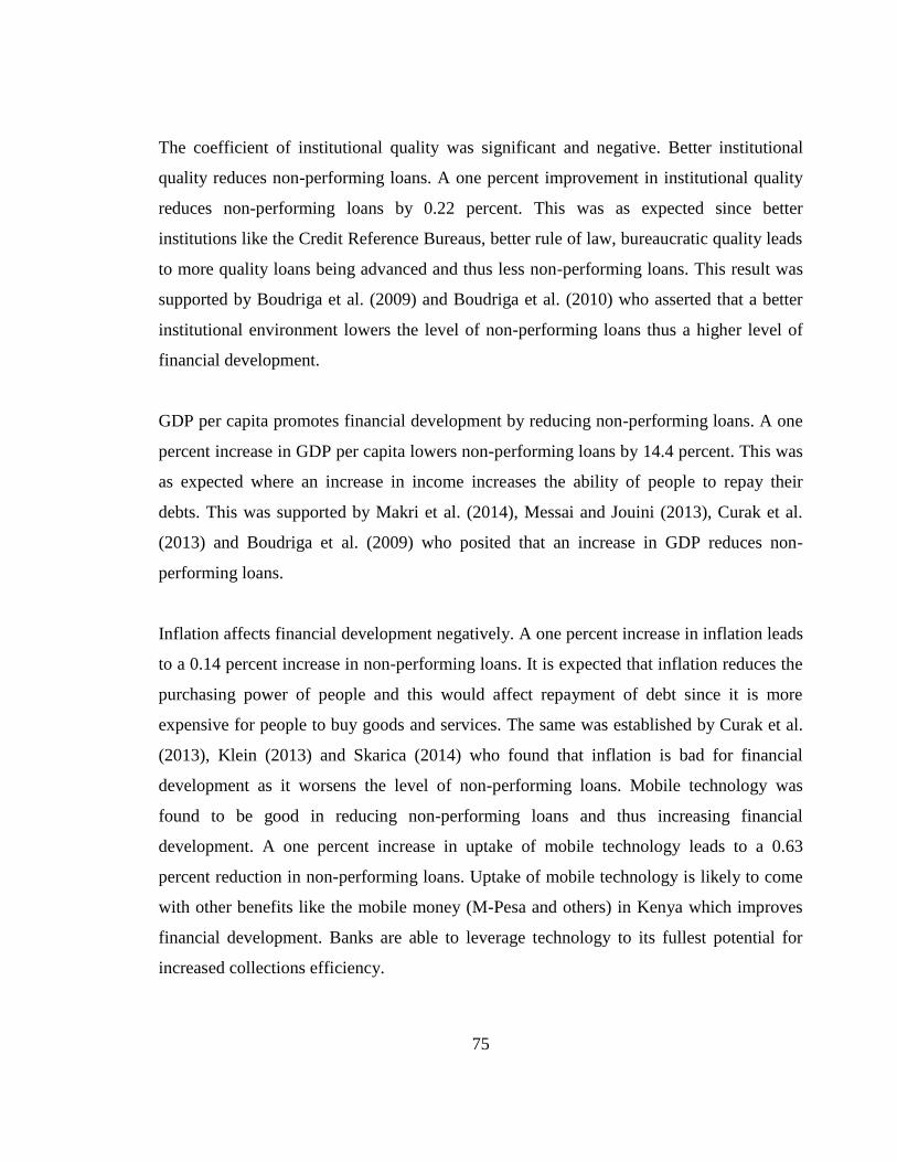
75
The coefficient of institutional quality was significant and negative. Better institutional
quality reduces non-performing loans. A one percent improvement in institutional quality
reduces non-performing loans by 0.22 percent. This was as expected since better
institutions like the Credit Reference Bureaus, better rule of law, bureaucratic quality leads
to more quality loans being advanced and thus less non-performing loans. This result was
supported by Boudriga et al. (2009) and Boudriga et al. (2010) who asserted that a better
institutional environment lowers the level of non-performing loans thus a higher level of
financial development.
GDP per capita promotes financial development by reducing non-performing loans. A one
percent increase in GDP per capita lowers non-performing loans by 14.4 percent. This was
as expected where an increase in income increases the ability of people to repay their
debts. This was supported by Makri et al. (2014), Messai and Jouini (2013), Curak et al.
(2013) and Boudriga et al. (2009) who posited that an increase in GDP reduces non-
performing loans.
Inflation affects financial development negatively. A one percent increase in inflation leads
to a 0.14 percent increase in non-performing loans. It is expected that inflation reduces the
purchasing power of people and this would affect repayment of debt since it is more
expensive for people to buy goods and services. The same was established by Curak et al.
(2013), Klein (2013) and Skarica (2014) who found that inflation is bad for financial
development as it worsens the level of non-performing loans. Mobile technology was
found to be good in reducing non-performing loans and thus increasing financial
development. A one percent increase in uptake of mobile technology leads to a 0.63
percent reduction in non-performing loans. Uptake of mobile technology is likely to come
with other benefits like the mobile money (M-Pesa and others) in Kenya which improves
financial development. Banks are able to leverage technology to its fullest potential for
increased collections efficiency.

76
The coefficients of trade openness, democratic accountability and remittances were
insignificant and hence the variables were not determinants of non-performing loans and
hence financial development. These results supported the economic institutions hypothesis
and rejected the openness hypothesis. The reason for rejection of openness hypothesis
could be due to the omission of financial openness which may work together with trade
openness to impact financial development (Rajan and Zingales, 2003 and Matadeen and
Seetanah, 2013). Further, trade openness may only impact financial development only if a
certain level of institutional quality is maintained (Chinn and Ito, 2005).
2.4.5 Error Correction Model Results
Due to the presence of cointegration, the study estimated the error correction models with
the differenced variables to bridge the long-run and short-run relationships. Table 2.8
reports the error correction estimates of the credit to private sector and non-performing
loans models. The short run variables were in differenced form while the long run
variables were at levels.

77
Table 2.8: ECM Estimates of Credit to Private Sector and Non-performing Loans Models
Credit to Private Sector MODEL Non-performing Loans MODEL
Variables Coefficient Coefficient
Short – Run Coefficients
Dependent Variable = DLNCredit to
Private Sector Dependent Variable = DLNNon-
Performing Loans
DLNCredit to Private Sector (-1)
-0.066
(0.093) -
DLNCredit to Private Sector (-2)
-0.556**
(0.109) -
DLNTrade Openness
0.042
(0.123)
-0.228
(0.194)
DLNTrade Openness (-1)
-0.740
(0.104) -
DLNTrade Openness (-2) -0.402** (0.108) -
DLNInstitutional Quality -0.033 (0.082)
-0.257** (0.151)
DLNGDP Per Capita 0.571
(0.683) -2.672** (1.202)
DLNInflation 0.043* (0.012)
0.045** (0.023)
DLNDemocratic Accountability
0.142**
(0.062)
-0.070
(0.119)
DLNRemittances
-0.282**
(0.133)
0.080
(0.068)
DLNTechnology
0.060**
(0.029)
-0.071
(0.045)
Error Correction Term - ECM(-1) -0.170** (0.025)
-0.104** (0.019)
Figures in parenthesis () indicate standard errors; * and ** indicates significance at 10% and 5% significance
level respectively.
Where D means difference while LN is natural logarithm. From the credit to private sector
model, the short run coefficients showed that the previous levels of credit to private sector,
trade openness, inflation, democratic accountability, remittances and technology are
significant determinants of credit to private sector. A one percent increase in trade
openness in lag two reduces credit to private sector by 0.03 percent. This short run finding
was in contrast to the long run finding that trade is good for financial development. As Do
and Levchenko (2004) found out, trade may not lead to financial development in poor
countries since they may import financial services rather than demand and develop their
own financial systems. A one percent increase in inflation, democratic accountability and
technology leads to a 0.04 percent, 0.14 percent and 0.06 percent increase in credit to
private sector respectively.
78
Remittances were found to reduce credit to private sector. A one percent increase in
remittances leads to a 0.28 percent reduction in credit to private sector. It is expected that
remittances would lead to uptake of more investments hence improvement in credit worth.
Ability to pay and credit worth would lead to increase in credit to the private sector.
Remittances may also be used for consumption and investment purposes and hence act as a
substitute to bank credit (Githaiga and Kibiru, 2014 and Giuliano and Ruiz-Arranz, 2000).
This could be the reason remittances impacted negatively on credit to private sector. The
coefficients of institutional quality and GDP per capita were significant and thus the two
variables were important determinants of financial development. The error correction
coefficient was negative and significant. The value of -0.17 showed a rapid adjustment
process with a disequilibrium or shock in the system taking six quarters or about one and a
half years to be restored to long –run equilibrium.
The short run coefficients of the non-performing loans model indicated that institutional
quality, GDP per capita and inflation were significant determinants of financial
development in the short run. A one percent increase or improvement in institutional
quality and GDP per capita reduces non-performing loans by 0.26 percent and 2.67 percent
respectively. However, an increase in the inflation rate by one percent increases non-
performing loans by 0.05 percent and thus lowering financial development. The error
correction term had a negative and significant coefficient of 0.10. This implied that when
there is a shock in the system, 10 percent of the shock is restored to equilibrium. So for the
whole disequilibrium to be adjusted to the long-run equilibrium, then the system needs ten
quarters or two and a half years.
2.4.5 Short Run Estimates of the Market Capitalization Model
The study found that there was no long run relationship in the market capitalization model.
The short run estimates of the market capitalization model were given in Table A.2
(Appendix). The results supported the economic institutions hypothesis that institutions are
important for financial development since the institutional quality coefficient is positive
79
and significant. Aduda et al. (2012) and Mbulawa (2015) found that higher institutional
quality promotes stock market development and hence financial development since better
institutions are able to guarantee security and protection of property rights for investors in
the stock market. The openness hypothesis was rejected since the trade openness
coefficient is insignificant. Huang and Temple (2005) and Chinn and Ito (2002) found that
trade openness promote financial development only in developed countries. In poor
countries it does not have an impact and if there is any impact then it can only be negative.
Klein and Olivei (2008) also found that trade openness is important for financial
development only in the presence of high institutional quality which is absent in
developing countries like Kenya. Other significant determinants of market capitalization as
an indicator of financial development included GDP per capita, democratic accountability
and technology which promote financial development. A one percent increase in GDP per
capita, democratic accountability and technology leads to a 2.84 percent, 0.57 percent and
0.15 percent increase in market capitalization respectively.
2.5 Conclusions and Policy Implications
This chapter set to determine the factors that influence financial development. The main
hypotheses tested were the endowment, economic institutions and the openness hypotheses
while controlling for other determinants of financial development. Three financial
development measures were used including credit to private sector, market capitalization
and non-performing loans. The ARDL model including the bounds test was used for
analysis. The findings showed that the three measures of financial development gave
distinct results and that the estimation results were sensitive to the choice of financial
development indicators.
The credit to private sector model supported the openness hypothesis as trade openness
was found to promote financial development in the long-run. In the short run, the effect
was negative. Therefore, economies should not expect immediate gains from trade. Higher
GDP per capita, better democratic accountability and higher uptake of mobile technology
80
were also found to promote financial development. Remittances were found to negatively
impact financial development only in the short run. The endowment and economic
institutions hypotheses were rejected since the coefficient of institutional quality was not
significant.
On the non-performing loans model, the endowment and economic institutions hypotheses
were supported as institutional quality coefficient was significant. However, the openness
hypothesis was rejected. Still, higher GDP per capita, less inflation, better democratic
accountability and more uptake of mobile technology were found to promote financial
development by reducing non-performing loans. No long-run relationships were found in
the market capitalization model but higher levels of institutional quality, GDP per capita,
democratic accountability and mobile technology were found to promote stock market
capitalization in the short run.
Deriving from the results of the three models, the results of the market capitalization were
weak since no long-run relationship was found between the variables. Hence, this study
relied on the results of the credit to private sector and non-performing loans models. It was
important to note that almost the same findings were found between the two models since
GDP per capita, democratic accountability and technology were significant determinants of
financial development in the long-run. However, the key distinct result was that credit to
private sector model supported the importance of trade openness (openness hypothesis)
while the non-performing loans model supported the importance of institutions (economic
institutions and endowment hypotheses). This was as expected since credit to private sector
shows the size of financial development and hence trade which increases the economic
activities of a country would then be key for financial development (Rajan and Zingales,
2003). Contrary, non-performing loans which indicate the quality of loans and efficiency
of the financial sector would be reduced if there are good institutions (Boudriga et al.,
2010). Thus, the two results were very important for the study. This was especially
81
important because the significance of institutional quality and relating it with the efficiency
of financial development is a new finding in Kenya.
Results indicated that institutional quality positively affected financial development since
the coefficient was significant. It is important especially for improving the quality of credit
in the financial sector which enhances financial development. Thus, policies that improve
the institutional environment should be pursued by the government and institutions. This is
especially important as institutional quality is considered low in Kenya. The government
should ensure proper functioning of legal and regulatory institutions to guarantee
protection of property rights and enforcement of credit contracts. There is also need to
have anti corruption policies to reduce corruption by increasing transparency in business
transactions and accountability. More credit reference bureaus should be introduced to
keep abreast with defaulters.
Trade was found to be significantly and positively related to financial development in the
credit to private sector model. Benefits from trade seem to be in the long-run and hence it
is important for policies to be directed at the long-term benefits of trade. Efforts should be
made by the government to reduce imports of financially dependent goods and services
and to promote exports. This should include not only primary exports as has been in Kenya
but also value added exports especially for agricultural products since they fetch better
earnings.
GDP per capita was positively related with financial development since the coefficient was
significant. The coefficient for inflation was also significant and negative. Thus, policies to
ensure a good macro-economic environment are important. Growth of the real economy is
important as it increases the GDP per capita of individuals. Strengthening legal and other
institutions, maintaining a good macro environment and improving human capital
development are some of the policies which can ensure continued growth in GDP per
82
capita. Policies to maintain inflation at threshold levels should be pursued by the Central
Bank including inflation targeting.
Democratic accountability coefficient was significant and positive. The political economy
is important for financial development as it promotes well functioning economic
institutions. Policies to improve the democratic accountability of Kenya should be pursued
including creating a conducive political environment, a more democratic government, a
system of political checks and balances, an increase in citizens‘ participation in financial
decisions, increased accountability and individual rights and reduced power held by
interest groups. So far, Kenya is doing well in terms of devolution which decentralizes
power for the benefit of the citizens and policies to tap into benefits of devolution should
continue. These include improved coordination mechanisms between the national and
county governments, capacity building for county governors and efforts to improve
governance at the county level.
Finally, mobile technology promotes financial development. The findings showed that the
coefficient of mobile technology was significant. Policies aimed at increasing the use of
mobile technology in the financial sector should be encouraged by the government. So far,
Kenya is leading in the use mobile money through M-Pesa. Such innovations should be
encouraged to tap fully into the benefits of technology. The Central Bank of Kenya has so
far ensured an enabling environment for banks to work with Safaricom Ltd and other
MNOs in advancing mobile banking.
2.6 Contribution of the Study
This study made three main contributions to knowledge. First it aimed at determining
drivers of financial development which has been ignored in Kenya. It introduced
institutional quality and political economy factors which have not been considered. The
study did this by testing three hypotheses: economic institutions, endowment and openness
hypotheses. The importance of institutional quality and political economy was supported

83
by the findings. Two, it introduced indicators of financial development which do not
necessary show the size and depth of financial development but rather its quality and
efficiency. This has been ignored in literature especially in African countries. The findings
showed that the quality and efficiency of financial development is important. Thirdly, the
study did not leave out the importance of mobile technology which has been key in the
wake of financial innovation in Kenya. Mobile technology was found to be significant for
financial development.
2.7 Limitation of the Study
The study was faced by limitations on data on the independent variables. Data on financial
openness was unavailable which may limit the results by biasing openness of a country to
trade and not capital/financial openness. Nonetheless, remittances would deal with this
problem as it is an aspect of financial openness. Further, data on some institutional quality
variables was unavailable. However, the used data was believed to be reliable for policy
recommendations.
2.8 Areas for Further Research Further analysi of the determinants of financial development ought to include an analysis
of threshold effects so as to determine at what level of the financial development indicators
one can say that a country is financially developed. With availability of more data, it is
important to capture the aspects of financial openness so as to avoid any biases in the
results. It would also be important to test the law and finance hypothesis and how it affects
financial development.
84
CHAPTER THREE
FINANCIAL DEVELOPMENT AND ECONOMIC GROWTH
3.1 Introduction
This chapter investigated the relationship between financial development and economic
growth. Having discussed the financial developments and innovations in Kenya, this
chapter endevoured to demonstrate how they are related to economic growth.
Several financial developments have occured in Kenya in the last decade. They include the
increase in number of bank branches, extension of bank operation hours, introduction of
Islamic banking, cross border banking, interbank trading, revised Prudential and Risk
Management Guidelines and the National Payment System Regulations enacted in 2014,
introduction of micro insurance schemes in the insurance industry, introduction of ATS,
new indices for the stock market and a trading platform for SMEs known as Growth
Emerging Markets Segments in the capital markets and new infrastructure bonds in the
bonds market. Additionally, there have been innovations in mobile payment services such
as M-Pesa which has been discussed in chapter one.
The growth of the financial sector has not been in tandem with economic growth. The
growth rate of the financial sector has been higher than the growth rate of the economy.
This growth in the financial sector has not been fully felt in the growth of the economy.
Globally financial sectors grow faster than the economy. Figure 3.1 compares the growth
rates of the financial sector and of the economy.
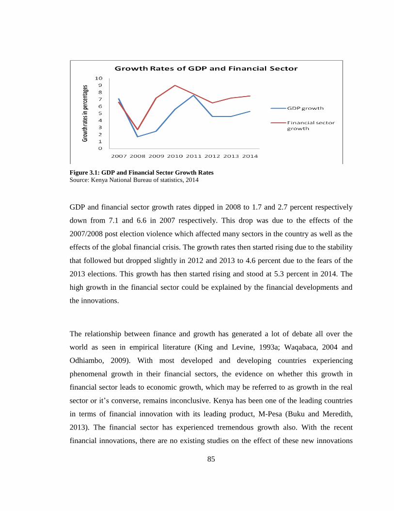
85
Figure 3.1: GDP and Financial Sector Growth Rates
Source: Kenya National Bureau of statistics, 2014
GDP and financial sector growth rates dipped in 2008 to 1.7 and 2.7 percent respectively
down from 7.1 and 6.6 in 2007 respectively. This drop was due to the effects of the
2007/2008 post election violence which affected many sectors in the country as well as the
effects of the global financial crisis. The growth rates then started rising due to the stability
that followed but dropped slightly in 2012 and 2013 to 4.6 percent due to the fears of the
2013 elections. This growth has then started rising and stood at 5.3 percent in 2014. The
high growth in the financial sector could be explained by the financial developments and
the innovations.
The relationship between finance and growth has generated a lot of debate all over the
world as seen in empirical literature (King and Levine, 1993a; Waqabaca, 2004 and
Odhiambo, 2009). With most developed and developing countries experiencing
phenomenal growth in their financial sectors, the evidence on whether this growth in
financial sector leads to economic growth, which may be referred to as growth in the real
sector or it‘s converse, remains inconclusive. Kenya has been one of the leading countries
in terms of financial innovation with its leading product, M-Pesa (Buku and Meredith,
2013). The financial sector has experienced tremendous growth also. With the recent
financial innovations, there are no existing studies on the effect of these new innovations

86
on economic growth. Further, the quality and efficiency of the financial sector have been
left out in determining the relation between financial development and growth, hence there
is a knowledge gap in Kenya which is yet to be addressed. Additionally, consensus is
lacking on the causality between these concepts in Kenya. Thus, the following questions
beg for answers which the study attempted to answer: How does financial development
affect economic growth when aspects of quality and efficiency are introduced?; How does
financial innovation affect economic growth?; What is the nature of the causal link
between financial development and economic growth?
The main objective of the study was to determine the relationship between financial
development and economic growth in Kenya.
Specifically, the chapter aimed at determining;
i) The effect of efficiency and qualitative aspects of financial development on
economic growth
ii) The effect of financial innovation on economic growth
iii) The nature of causality between financial development and economic growth
3.1.1 Significance of the Study
The study is important in terms of providing knowledge on whether financial development
is crucial for economic growth or the vice versa. This is important for policy decision
making with respect to targeting the growth of the financial sector or overall economic
growth. Further, knowing how financial innovations affect economic growth is important
to policy makers in deciding how to support innovations. This is especially in terms of the
legal and regulatory framework, gaining legitimacy and how they can be integrated into the
wider financial system. The gap of disregarding the quality and efficiency aspects of
financial development in the finance-growth relationship is important to policy makers
since they can work on improving these aspects. The study is also important to existing
literature and for future researchers in the finance-growth nexus especially in giving more
clarity on the causality between financial development and growth and expanding the
87
definition of financial development to include financial innovation and the quality and
efficiency aspects.
3.2 Literature Review
3.2.1 Theoretical Literature
The seminal literature on finance and growth is due to Schumpeter (1911). Schumpeter
argued that financial intermediation through the banking channel plays an important role in
economic growth and development. The effect is through the allocation of savings from
the ones who have to the ones who do not and thus increasing productivity, technical
progress and thus improving economic growth.
Another theory linking financial development to economic growth is what Mckinnon
called ‗conduit effect‘ (Mckinnon, 1973). The theory posits that financial development
leads to growth in domestic savings which further leads to increase in investments. In this
theory, investment is related positively to the real interest rate. This is because a high
interest rate leads to an increase in domestic savings which then avails funds for
investment. An increase in investment further enhances growth. This view is supported by
Shaw (1973).
The theory behind finance and growth can also be derived from the neoclassical growth
model introduced by Solow and Swan (1956) which posits that long-run growth is
explained by capital accumulation, labour productivity and technical progress. Thus, the
link between finance and growth can be explained by incorporating financial development
into the simple neoclassical model (King and Levine, 1993; Easterly and Levine, 1994 and
Elbadawa and Ndulu, 1994). Thus, from the simple production function, financial
development variables are added as shift parameters in addition to the usual factors of
production to form the unrestricted neoclassical growth model. However, the neoclassical
growth model is limited due to the fact that technology is treated as an exogenous factor.
Therefore, the endogenous growth theory is better in explaining the relationship between

88
finance and growth (Loayza and Ranciere, 2006). Technology, through which financial
development enters the model, is treated as an endogenous factor affecting growth.
One of the endogenous growth theories linking finance and economic growth is the AK
endogenous growth model introduced by Pagano (1993). The theory propounds that output
is a linear function of capital accumulation or capital stock resulting in a production
function given by: tt AKY , Where Yt is economic growth, Kt is capital stock and A is
capital productivity. This model was extended by Romer (1989) in which each firm faces
technical progress with constant returns to scale and productivity is an increasing function
of capital. Pagano (1993) then assumed that a proportion of savings is lost in the process of
intermediation 1 such that in a closed economy where savings equals investment,
then tt IS . The Pagano AK endogenous growth model eventually reduces to
sAg concluding that finance affects economic growth by reducing the proportion of
resources that is lost in allocating capital, by increasing the savings ratio and increasing the
capital productivity.
In regards to the theoretical models between finance and growth, the various propositions
of the theories differ along three distinct aspects which include the source of endogenous
growth, the finance mechanism and the way asymmetric information is handled (Trew,
2006). In regards to the source of endogenous growth, the sources identified include;
production externalities, vertical externalities, horizontal externalities, capital and human
capital externalities. The finance mechanisms mainly include banking system/credit
markets, capital markets, insurance markets and entrepreneurship funding. Information
asymmetry includes adverse selection and moral hazard and also presence of exogenous
productivity and liquidity shocks. In most of these models it is clear that the main
hindrance to growth is credit or financial constraint in the acquisition of knowledge and
technology.

89
Theory also gives two channels through which financial development connect with
economic growth which are risk sharing and information asymmetry. Investors in trying to
allocate capital to the most profitable investments, usually face information constraints and
they do not always have the capacity to collect all the necessary information so as to invest
in the most profitable investments. Acquiring information to ensure more optimal resource
allocations is costly and hence a challenge. As such, financial intermediaries improve
resource allocation by reducing the costs of information acquisition (Allen, 1990). They
collect information on behalf of investors and thus investors can make informed decisions
based on expected returns thus weeding out the weak projects. However, financial
intermediaries may be limited due to limited information on investment opportunities
resulting from a large informal sector.
On the other hand, risk sharing plays an important role in promotion of economic growth if
the agents are risk averse and less risky projects yield low returns. The financial system
allows agents to diversify their portfolios with those that have higher expected yields while
maintaining reasonably low risks (Greenwood and Jovanovic, 1990; Obstfeld, 1994 and
Schumpeter, 2011). This increases investment returns as well as allowing for better allocation
of resources and thus impacting growth. Further, risk sharing plays a critical role also when
economic agents face liquidity risks. Agents, In addition to being averse to risks will want to
hold some of their savings in liquid assets. Thus, the financial system can play a role in
ensuring maintenance of liquidity and ensuring that projects are generally acceptable thus
promoting growth (Diamond and Dybvig, 1983).
Further, a reverse or feedback mechanism exists from economic growth to finance
development. Economic activity can have an effect on financial systems. Financial
development is seen as a consequence of a growing economy (Robinson, 1952 and Patrick,
1966). A growing economy leads to increased demand for financial services and instruments.
Patrick (1966) termed this as demand following financial development while Robinson (1952)
called it the growth led finance. Further, Patrick (1966) postulated that there could be a two
way relationship not just the demand following hypothesis but also a reverse causation
90
between finance and growth. Another route growth impacts financial development is through
the growth of institutions (Trew, 2006). Increased demand in the economy leads to set up of
new financial institutions, their growth and innovations.
3.2.2 Empirical Literature
a) Relationship between Financial Development and Economic Growth
Three views exist in the empirical literature regarding the relationship between financial
development and economic growth. The first view argues that financial development is
important and leads to economic growth (supply-leading hypothesis). The second view
postulates that it is economic growth that drives the development of the financial sector
(demand-following hypothesis) while the third view contends that both financial
development and economic growth Granger-cause each other, i.e., there is a bidirectional
causality between financial development and economic growth. The studies that supported
the supply-leading hypothesis include: Jung (1986), Crichton and De Silva (1989), King
and Levine (1993), DeGregoria and Guidotti (1995), Odedokun (1996), Levine and Zervos
(1998), Rajan and Zingale (1998), Odhiambo (2002), Habibullah and Eng (2006),
Odhiambo (2009c) and Uddin et al. (2013a).
In regards to the supply leading hypothesis, this finding is reached even with the use of
different methodologies, different type of data as well as different areas of study. Financial
development is seen to be important for economic growth in various ways. One of the
ways this happens is through innovation (King and Levine, 1993). Innovations do improve
the usual way of doing things and thus increases productivity. However, distortions in the
financial sector are seen to reduce innovation and hence growth. Financial market
development in contributing to growth leads to reduced costs of external finance to firms
(Rajan and Zingales, 1998). Industrial sectors that depend more on external finance thrive
well in countries with better developed financial sectors and thus financial market
development is crucial for economic growth. Another view supported by Habibullah and

91
Eng (2006) is the ―financial structuralist‖ view which postulated a significant broad
presence of financial institutions and growth of financial instruments will lead to higher
growth.
Savings and investment were found to be important in raising economic growth (Xu, 2000
and Suleiman and Abu-Qaun, 2008). This proposition is in support of the Mckinnon
conduit effect. The financial sector development encourages savings which in turn
encourage investments and thus growth. Japelli and Pagano (1994) and De Gregoria and
Guidotti (1995) also supported the importance of savings in growth. De Gregoria and
Guidotti (1995) however noted that poor regulation of financial markets can lead to
negative effects on economic growth. As regards to the Pagano (1993) A.K model, some
studies have indicated that financial development affects growth through the allocative
efficiency where better allocative efficiency improves investment (Greenwood and
Jovanovic, 1990; Bencivenga and Smith, 1991 and Levine, 1991). Efficiency is another
way financial development affects economic growth (Graff and Karmann, 2006). When
resources are allocated efficiently without wastages, this is likely to cause higher and faster
growth.
In Kenya, several studies have been carried out and found support for the supply leading
hypothesis. Odhiambo (2002) was among the first studies who found support for supply
leading hypothesis. Mckinnon hypothesis was found to exist in Kenya with introduction
savings. Savings are seen to be important for capital accumulation hence growth. In
Odhiambo (2009c), lack of a conclusion on the relationship between finance and growth
led to introduction of interest rate reforms as a new variable in the analysis. Interest rate
reforms which support financial development led to growth. Other studies which supported
the role of savings (through growth in the financial sector) in fuelling economic growth
include Uddin et al. (2013a).
92
The second hypothesis which is the demand following hypothesis is supported by several
studies. These studies included Shan et al. (2001); Agbetsiafa (2003); Waqabaca (2004);
Odhiambo (2004); Ang and McKibbin (2007); Odhiambo (2008a, 2009b) and Gautam,
2014). Economic growth provides a conducive environment for the growth of financial
sector since it creates higher demand for financial services (Shan et al., 2001; Agbetsiafa,
2003). Countries with less sophisticated and lowly developed financial sectors likely find
that it is economic growth that leads to the development of the financial sector (Waqabaca,
2004 and Ang and McKibbin, 2007). In Kenya, the importance of economic growth for
financial development was shown by Agbetsiafa (2003) and Odhiambo (2004, 2008a,
2009c). Odhiambo (2009b) controlled for inflation and still found a demand following
hypothesis support. These Kenyan studies used the same financial development mainly
broad money supply.
Other findings support neither the supply-leading hypothesis nor the demand-following
hypothesis. They have shown that financial development and economic growth can
Granger-cause one another, that is, a bi-directional relationship. Jung (1986), Wood
(1993), Akinboade (1998), Kar and Pentecost (2000), Calderon and Liu (2003), Chuah and
Thai (2004) found support that demand following hypothesis usually holds mostly for
developed countries in contrast to the developing countries. This is because developed
countries are likely to have more developed financial sectors even with low growth rates.
The good conditions, better facilities act as a further catalyst for the growth of the financial
sectors. However, in Kenya, which is a developing country, similar findings of both the
demand following hypothesis and supply leading were reached (Odhiambo, 2005;
Odhiambo, 2008a; Wolde – Rufael, 2009 and Onuonga, 2014). These findings could have
been arrived at due to the use of poor financial development indicators which are
applicable for developed countries like broad money supply. Most of the other studies used
the same financial development indicator, for example Gautum (2014) using M2 found a
bi-directional relationship between finance and growth in Nepal.
93
b) Data and Methodology
Various studies have reached different conclusions based on the methodologies and the
types of data used. Jung (1986) and King and Levine (1993) used cross sectional data and
OLS method of analysis and concluded that financial development positively influences
economic growth. However, OLS does not control for endogeneity and other methods like
the GMM-IV methods are able to deal with this problem (Beck et al., 2000 and Gehringer,
2013). Other panel data analysis found different results. Panel data is advantageous
especially because of low data availability for long periods in many countries. De Gregoria
and Guidotti (1995) and Rajan and Zingale (1998) using OLS and fixed effects model
found support for the supply leading hypothesis between financial development and
economic growth. However, Calderon and Liu (2003) used panel data and applied the
VAR methodology and granger causality methods and found a bi-directional relationship
between financial development and growth. Panel data GMM estimations were used to
find the supply leading hypothesis by Habibulla and Eng (2006).
Time series country specific analysis have been found to be advantageous especially when
forecasting is necessary (Ang and McKibbin, 2007). Multivariate time series analysis also
deals with endogeneity problems common in cross sectional and panel data analysis
(Neusser and Kugler, 1998). Time series analysis has been carried out with different
findings. The main methods of analysis with time series data include Cointegration,
granger causality testing, Hsiao causal testing approach (Hsiao, 1979), VAR, VECM,
ECM and ARDL. Xu (2000), Odhiambo (2002), Habibullah and Eng (2006), Uddin et al.
(2013a) and Mittal (2014) all found support for the supply leading hypothesis using time
series data. Other country specific studies found support for demand following
(Agbetsiafa, 2003; Waqabaca, 2004; Ang and McKibbin, 2007; Odhiambo, 2009 and
Gautam, 2014). Finally, those who found a bi-directional relationship using time series
analysis included Luintel and Khan (1996), Akinboade (1998), Odhiambo (2008a), Wolde
– Rufael (2009) and Onuonga (2014). There are several studies done in Kenya using time
series and they all found different results which could be as a result of use of different
94
financial development indicators (Odhiambo, 2008a; Wolde – Rufael, 2009 and Onuonga,
2014).
c) Measurement of Financial Development
The use of different financial development indicators have led to different findings.
Starting with Goldsmith (1969), they used the value of deposits to GDP. This measure was
criticized as it is very simplified and does not assess the direction of causality. Further,
King and Levine (1993a) used several indicators of financial development including liquid
liabilities as a percentage of GDP, credit allocation of commercial banks relative to Central
bank, domestic credit to GDP and credit to private sector to total domestic credit and found
strong support that financial development is good for the growth of the economy. Levine
and Zervos (1998) used some of these measures and found support for supply leading
hypothesis. However, Rajan and Zingales (1998) criticized these measures as they just
reflect the level of financial development in terms of credit allocated and money supply.
They used capitalization measures and the accounting standards which indicate possibility
of obtaining finance instead of looking at just the finance secured and found that financial
development is important for economic growth through reduction of costs of finance and
rise of new firms which come with new sources of ideas.
This measurement issue has been discussed in literature with many criticizing some of the
financial indicators used. One of the indicators of financial development which has been
criticized is the broad money supply, M2 or M3. This indicator has been used in several
studies (Odhiambo, 2002; Agbetsiafa, 2003; Odhiambo, 2009; Wolde-Rufael, 2009,
Akinlo and Egbetunde, 2010 and Gautam, 2014). This measure is criticized because it does
not show the capacity of the financial sector to provide savings for investment (Ang and
Mckibbin, 2007 and Gehringer, 2013). It mainly shows the overall stock of money in
circulation and other liquid assets not necessarily what is available for investment (Khan
and Senhadji, 2003). This measure is also criticized for use in low income countries since
currency in circulation which makes the highest proportion of M2 is high (Dushku, 2010).
95
Adnan (2011) recommended that currency in circulation ought to be removed from the
broad money supply if it has to be used as a measure of financial development because an
increase in broad money supply basically implies an increase in currency in circulation.
Assets by commercial banks as a ratio of assets by commercial banks plus central banks
assets as used by King and Levine (1993) has also been criticized since it shows the
relevance of commercial banks in intermediation better than Central banks can do.
However, this measure only shows the financial intermediation but does not indicate the
quality of the financial sector in intermediation (Gehringer, 2013). Another measure that
has been criticized is the use of domestic credit as a ratio of GDP as it includes credit even
to the public sector which is assumed not to be as efficient in allocating resources unlike
the private sector (Ayadi et al., 2013). Therefore, literature suggests the use of credit to
private sector which implies more efficient allocation of resources (Liang and Teng, 2006;
Adamopoulos, 2010; Arcand et al., 2011).
To avoid all the criticisms of the use of these indicators, several studies have used a
financial development index calculated through the Principal Component Method (Ang
and McKibbin (2007), Kargbo and Adamu (2010), Adnan (2011), Uddin et al. (2013a),
Dhrifi (2013). They supported the use of a financial index since the use of the various
indicators of financial development are not exhaustive and do not fully cover financial
development especially in the bonds market, pension funds and insurance markets.
Neusser and Krugler (1998) in critiquing the various measures of financial development
including the index proposed the use of the GDP of the financial sector because it
encompasses the various aspects of financial development. They argued that financial
activities are not just from the banking institutions but include activities from pension
funds, investment banks, security brokers, insurance dealers and thus, the GDP of the
financial sector would be a good measure of financial development. However, the same
studies criticized this measure as being too broad and it does not show the specific

96
contributions from the various intermediation institutions hence specific policy cannot be
inferred.
The use of a financial index has been criticised as the process of creating one leads to loss
of information which would be better captured by individual indicators (Neusser and
Krugler, 1998). These indicators show the financial depth, the liquidity of the banking
sector, return on savings as well as the contribution of non-bank sectors. These also do not
show how savings are converted into investments. They further do not show the quality of
financial development but just just the quantity. Therefore, with the strong critic of the
various measures, the study takes a broader definition of financial development. Financial
development should not only show the expansion of the financial sector in terms of
quantity, it is also important to show the quality and efficiency of this expansion. From the
above discussion, the efficiency and quality of financial development seem to have been
ignored while it has been raised as important in the relationship between financial
development and poverty (Dhrifi, 2013). Thus, it was important to include these aspects of
financial development in the relationship between financial development and poverty.
Thus, the study adopts new financial development indicators including non-performing
loans and interest rate spread as well as credit to private to show how savings are converted
to investment.
d) Use of Efficiency and Quality Indicators of Financial Development
The use of various financial development indicators has led to conflicting results as
discussed. Literature has evolved to include the importance of efficiency measures of
financial development in determining the relationship between financial development and
economic growth. Koivu (2002) pointed out that when efficiency of the financial sector is
ignored, then findings are likely to give the wrong effects and causality between financial
development and economic growth. The study argued that indicators that measure the size
of the financial sector only like domestic credit could be better used in developed
economies since the quantity of the financial sector may be correlated with its efficiency
97
and both of them are high in developed economies. Therefore, using only the quantity of
the financial sector in developing economies does not fully give us the correct relationship
between financial development and economic growth as it does not show us the efficiency
of the sector. Further, mere growth in the quantity of the financial sector cannot be
considered as financial development. Adnan (2011) and Ayadi et al. (2013) also indicated
the importance of the efficiency of the banking sector in allocating resources which is
important as mere quantity of intermediation may not show financial development.
The qualitative development of the financial sector is important and aspects like
transaction costs and the quality of information the banking sector collects are well
explained by indicators which show the quality of the financial sector (Dudian and Popa,
2013). Qualitative as well as quantitative aspects of the financial sector should be
considered since growth in the quantitative aspects may not be accompanied by a similar
growth in the quality of the growth hence undermining the overall effect. Non-performing
loans and interest rate spread represents qualitative and efficiency aspects. Quality of the
financial sector development is important for economic growth while the quantity of the
development is less relevant in transition economies (Dudian and Popa, 2013).
Efficiency of the financial sector as indicated by high collateral and low transaction costs
is lower in low income countries as compared to emerging and developed economies
(Dabla-Norris et al., 2014). The study found that GDP responds to lower transactions costs
and thus these measures are important for economic growth. This study thus in expanding
the definition of financial development to include the quality and efficiency included two
measures to show this. One is the non-performing loans which show the quality of credit
and hence may indicate the quality of financial development. Secondly, the study used the
interest rate spread which shows the transaction costs in the process of financial
intermediation. A higher interest rate spread would imply higher inefficiency in the
financial sector. Thus, the study adopted these two measures in the analysis.

98
e) Use of Bank Based or Stock Market Based Financial Development Indicators
In addition to literature on causality and effect of financial development and growth, the
role of bank based and market based financial systems has been highlighted in literature
(Levine, 2003 and Adebola and Dahalan, 2011). Some countries like Germany and Japan
have developed based on the banking sector while others like the US and England have
developed based more on the stock market hence the importance of these two industries is
critical. Several studies have been undertaken on the relationship between financial
development due to the stock market and economic growth (Nagaraj, 1996; Levine and
Zervos, 1996; Tadesse, 2002 and Yartey, 2007) and on financial development based on the
banking industry and growth (Odhiambo, 2008a and Odhiambo, 2009b). Some of these
studies also supported the importance of both systems. Yartey (2007), for example,
concluded that both the banking sector and the stock market are important for economic
growth. The study posited that a well functioning banking sector can support growth in the
stock market while a stock market that is vibrant can improve performance of the banking
sector and hence encourage growth.
Levine and Zervos (1996) using cross country analysis asserted that the stock market is
important since it offers what the banking sector cannot offer. Credible examples include
equity finance which is a form of long term finance that can influence investment and
growth. This equity finance is less sensitive to the effects of moral hazard and adverse
selection and thus better in leading growth. Singh (1997) criticized the disregard of the
importance of the stock market for economic growth and concludes that they play an
important role in both domestic and foreign liberalization. Stock markets (due to increased
liquidity) can also influence growth negatively. This effect occurs through three channels
which include reducing savings rate due to increased liquidity, increasing uncertainty on
savings as well as the benefits from a perky stock market (Arestis et al., 2001). Studies
which supported stock markets‘ importance on economic growth in Kenya include Olweny
and Kimani (2011). Using the cointegration approach and granger causality, they found a
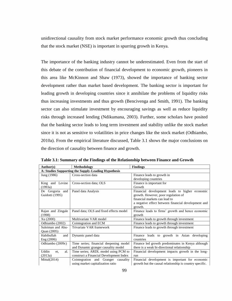
99
unidirectional causality from stock market performance economic growth thus concluding
that the stock market (NSE) is important in spurring growth in Kenya.
The importance of the banking industry cannot be underestimated. Even from the start of
this debate of the contribution of financial development to economic growth, pioneers in
this area like McKinnon and Shaw (1973), showed the importance of banking sector
development rather than market based development. The banking sector is important for
leading growth in developing countries since it annihilate the problems of liquidity risks
thus increasing investments and thus growth (Bencivenga and Smith, 1991). The banking
sector can also stimulate investment by encouraging savings as well as reduce liquidity
risks through increased lending (Ndikumana, 2003). Further, some scholars have posited
that the banking sector leads to long term investment and stability unlike the stock market
since it is not as sensitive to volatilities in price changes like the stock market (Odhiambo,
2010a). From the empirical literature discussed, Table 3.1 shows the major conclusions on
the direction of causality between finance and growth.
Table 3.1: Summary of the Findings of the Relationship between Finance and Growth
Author(s) Methodology Findings
A: Studies Supporting the Supply-Leading Hypothesis
Jung (1986) Cross-section data Finance leads to growth in
developing countries
King and Levine
(1993a)
Cross-section data; OLS Finance is important for
Growth
De Gregoria and
Guidotti (1995)
Panel data Analysis Financial development leads to higher economic
growth. However, poor regulation of
financial markets can lead to
a negative effect between financial development and
growth.
Rajan and Zingale
(1998)
Panel data; OLS and fixed effects model Finance leads to firms‘ growth and hence economic
growth
Xu (2000) Multivariate VAR model Finance leads to growth through investment
Odhiambo (2002) Cointegration and ECM Finance leads to growth through investment
Suleiman and Abu-
Quan (2005)
Trivariate VAR framework Finance leads to growth through investment
Habibullah and
Eng (2006)
Dynamic panel data Finance leads to growth in Asian developing
countries
Odhiambo (2009c) Time series; financial deepening model
and Dynamic granger causality model
Finance led growth predominates in Kenya although
there is a weak bi-directional relationship
Uddin et, al.
(2013a)
Time series; ARDL model using PCM to
construct a Financial Development Index
Financial development impacts growth in the long-
run
Mittal(2014) Cointegration and Granger causality
using market capitalization ratio
Financial development is important for economic
growth but the causal relationship is country specific.

100
Table 3.1 continued
B: Studies Supporting the Demand-Following Hypothesis
Agbetsiafa (2003) Time series; VECM Economic growth leads to Financial development in
Kenya and Ivory Cost
Waqabaca, (2004) Time series; Bivariate
autoregressive framework
Growth precedes financial development
Odhiambo (2004) Time series; Bivariate
causality test based on ECM
Economic growth leads to Financial development in
South Africa and Kenya
Ang and Mckibbin
(2007)
Time series; VECM,
Cointegration, granger
causality and PCA
Economic growth leads to financial development in the
long-run
Odhiambo (2008a) Time series; Cointegration and ECM Demand following hypothesis dominates in Kenya
Odhiambo (2008b) Time series; Trivariate
causality test based on ECM
Growth leads finance
Odhiambo (2009b) Time series; Trivariate
causality test based on ECM
Unidirectional causality from growth to finance
Gautam (2014 VECM and Granger Causality Growth leads financial development in Nepal
C: Studies Showing a Bi-directional Causality between Finance and Growth
Wood (1993) Time series; Hsiao causal testing
approach
Bi-directional causality between finance and growth
Luintel and Khan
(1996)
Time series; Multivariate VAR
framework, VECM
Bi-directional causality between finance and growth
Akinboade (1998) Time series Bi-directional causality between finance and growth
Calderon and Liu
(2003)
Panel data analysis; VAR,
Geweke decomposition and
Granger causality models
Bi-directional causality between finance and growth.
However, the finance effect on growth is higher in
developing countries than in developed countries
Odhiambo (2005) Time series; Bivariate
causality test based on ECM
Bi-directional causality between finance and growth in
Tanzania
Wolde-Rufael, 2009 Time series: Quadvariate
VAR framework
Bi-directional causality between finance and growth in
Kenya
Akinlo and
Egbetunde (2010)
Time series; Multivariate
cointegration analysis and
ECM
Bi-directional causality in Kenya, Chad, South Africa,
Sierraleone and Swaziland. However, finance is found
to precede growth in Central African Republic, Congo,
Gabon and Nigeria while the demand following
hypothesis is found in Zambia.
Onuonga (2014) ARDL Both financial development and economic growth
influences each other in Kenya
3.2.3 Overview of the Literature
Different theories on the relationship between finance and growth are supported due to
methodologies used, indicators of financial development used and country of study. The
literature concluded that three types of relationships between financial development and
economic growth exists; supply leading, demand following and a bi-directional
relationship. Despite the literature giving divergent views on the importance of the banking
industry as well as the stock market, both of these industries are seen to be important
indicators of financial development. For this reason, the study included bank and stock
101
market variables. With the literature supporting these three views, two questions are; what
if there exists no relationship between financial development and economic growth? is
economic growth caused by other variables other than financial development?
Secondly, the studies that have been done in Kenya (Odhiambo, 2008, 2009 and Wolde
Rufael, 2009) in their analyses of financial development and growth used financial
development indicators/variables which are applicable to developed countries. For
example, M2 or M3 is a monetization measure representing financial depth. M3 composes
M1, M2 and long term time deposits, institutional money market funds and repurchase
agreements. Generally, this is a good measure of financial development in developed
countries as the level of M1 is low. However, in underdeveloped countries, currency in
circulation, that is currency held outside the banking system, makes the highest percentage
of M2 and M3 and thus they would not be good measures of financial development
(Dushku, 2010). This is supported by researchers who have argued that M2 and M3 are
poor measures of financial development in underdeveloped countries as the high
monetization may be linked to underdevelopment in the financial sector (De Gregorio and
Guidotti, 1995). In addition, M2 mostly reflects the extent of financial services provided
by the financial system instead of the ability of the financial system to channel funds from
those who have (depositors) to those who do not (Khan and Senhadji, 2003). A good
substitute for this monetization measure in underdeveloped countries would be liquid
liabilities of banks to GDP (Dushku, 2010) as it excludes currency outside banks which is
high in underdeveloped countries.
Domestic credit may also not be a good measure of financial development as used by most
studies done for Kenya (Adamopoulos, 2010; Arcand et al., 2011). This includes domestic
credit by all institutions to both public and private sectors. This measure is quite broad and
since not all funds given out are used for investment, narrowing down to bank credit to
private sector helps us to concentrate on those funds that go for investment purposes by the
private sector. The private sector is deemed to be more competitive than the public sector

102
and thus funds may be used more efficiently and lead to Pareto optimal allocation of
resources. Thus, Bank credit to private sector is a good indicator of financial development
as it shows the ability of the financial system to channel funds from the surplus to deficit
agents through the banking system (Levine and Zervos, 1998; Liang and Teng, 2006;
Adamopoulos, 2010; Arcand et al., 2011). It shows the general level of development in the
banking sector (Ayadi et al., 2013).
This study thus made a diversion on the indicators used previously to represent financial
development to use Liquid Liabilities of banks which excludes currency instead of Money
supply measure (M2 or M3), bank credit to private sector instead of domestic credit to
private sector. Other variables to represent efficiency and quality of the financial sector
included non-performing loans and interest rate spread which have been ignored before in
the earlier studies in Kenya. Non-Performing Loans (NPLs) can be used as a proxy for
efficiency since an efficient banking system would be expected to have low NPLs while
interest rate spread shows the transaction costs of channeling funds to investment. These
variables were as suggested in literature (Koivu, 2002 and Dudian and Popa, 2013) to
incorporate the qualitative and efficiency aspects of financial development.
None of the studies done in Kenya has included a measure of financial innovation even
with all the financial innovations that have taken place in Kenya in the last couple of years.
Therefore, this study included mobile payments as a measure of financial innovation in the
financial development and growth equation. Further, presence of structural breaks in the
variables may lead to distortion of results where a unit root may be rejected and it is
present due to the influence of structural breaks. Most of the studies especially those that
have been done in Kenya had not taken into consideration the distortions which would be
brought about by presence of structural breaks in the data. Thus, this study went further to
consider structural breaks.
103
3.3 Methodology
3.3.1 Theoretical Framework
The relationship between finance and growth can be derived from the Pagano ‗AK‘
endogenous growth model (Pagano, 1993) where output is a linear function of capital stock
giving a reduced form production function resulting from Romer (1989) where each firm
faces technical progress with constant returns to scale and productivity increasing with
capital.
tt AKY .............................................................................................................................3.1
Changes in capital stock which leads us to investment is given by gross investment less
depreciation of capital stock ( )
tttt KIKK 1 ……………………...………………………………………………..3.2
Then gross investment becomes;
ttt KKI )1(1 ……………………...……………………………………………….3.3
In a closed economy, equilibrium requires that Savings equals Investment. However,
Pagano assumes that a proportion of 1 is lost during the process of financial
intermediation and thus equilibrium becomes:
tt IS ……………………………………………..…………………………………......3.4
Introducing growth rates and using equations 3.1, 3.2 and 3.3, the steady state growth rate
of output is derived as follows:

104
At steady state, growth rate of output is the same as growth rate of capital since marginal
productivity of capital absorbs all depreciation, growth rate at time 1t is: 1tg =
t
tt
Y
YY 1 = 11
t
t
Y
Y= 11
t
t
K
K
…………………………………………………………….3.5
Where 1tg is the growth of output in time t+1.
Using equation 3.1, tt AKY then 11 tt AKY……………………….……………….3.6
From equation 3.3, ttt KIK )1(1 …………………………….………………….3.7
Then, substituting for 1tK , ))1((1 ttt KIAY …………………………………..3.8
Applying the growth rates:
1))1((
11
t
tt
t
t
Y
KIA
Y
Y
………………….………………………………………3.9
Replacing tI using equation 3.4, using t
t
K
YA (from equation 3.1) and the fact that t
t
t sY
S
1
))1((
t
tt
t
t
tY
KIK
Y
g
…………………………………………………………….3.10
= ])1([1
. tt
tt
t KSYK
Y ……………………………………………………………….3.11
= 1)]1([ t
t
K
S……………………………………………………………………3.12
= 1)]1(.[ t
t
t
t
K
Y
Y
S……………………………………………….…………….....3.13

105
dropping the time indices, then:
sAg ……………………………………….……….…………………………..3.14
Where g is economic growth, s is the saving rate denoted by S/Y. Thus, output growth is
influenced by , the proportion of savings channeled to investment, s, the saving rate and
A, the social marginal productivity of capital. According to Pagano, 1993 financial
development can affect growth through these three variables; it can raise the proportion of
savings channeled to investment, it may increase the marginal productivity of capital or
influence savings. Thus financial sector development ―has not only a level effect but also a
growth effect‖, as it affects economic growth not only through savings but also the
marginal productivity of capital.
Assuming zero depreciation, equation 3.14 gives the Pagano endogenous growth model as:
sAg …………………………………………………………..……………………3.15
3.3.2 Empirical Model
The study aimed at estimating the effect of financial development on economic growth as
well as determining the causality between financial development and economic growth.
Deriving our model from the Pagano ‗AK‘ endogenous growth model described in section
3.3.1 where output is a linear function of capital stock, a reduced form equation is obtained
as: sAg
Where financial development indicators were included to capture A and . The variables
used here either represented A, which is the allocative efficiency/productivity of capital, ,
which is the proportion of savings channeled to investment and s, the savings rate. Non-
performing loans as a percentage of total loans and Bank credit to Private sector represent
allocative efficiency (A) while interest rate spread influences the proportion of savings
channeled to investment ( ) and captures transaction costs for financial intermediation.
Liquid liabilities of banks and market capitalization represent the quantity of financial
106
development. Liquid liabilities of banks includes M2 less currency in circulation, bank
credit to private sector is a measure of financial depth but isolates credit given by other
financial institutions and credit to the public sector. It is thus the most important measure
of financial intermediary development, (Levine and Zervos, 1998 and Yartey, 2007).
The study assumed that the private sector is more competitive than the public sector.
Therefore, according to the first theorem of welfare economics, it (competitive markets)
leads to more Pareto efficient allocation of resources (a restatement of the Adam smith‘s
invisible hand theorem). Thus, giving credit to the private sector in contrast to the public
sector would lead to more Pareto efficient outcomes. NPLs as a percentage of total loans is
a measure of the quality of financial assets hence quality of financial development while
interest rate spread is the difference between borrowing and lending rates by financial
institutions.
A measure of financial innovation in the form of mobile payments was included.
According to Krishnan (2011), financial development is broad and includes three pillars:
The policies, factors, institutions and innovations that allow for effective financial
intermediation; The size, depth and efficiency of the financial intermediaries and the
institutions/markets that provide financial services and: Financial access which involves
access of individuals and business to financial services as well as credit/capital. Mobile
money services as a financial innovation allow people to have access to new financial
services. In this study, mobile money services were represented by M-Pesa which is one of
the innovations discussed in chapter one. Thus, this study went beyond the traditional
measures of financial development which are size and intermediation, to include new
indicators of financial development which can be divided into efficiency and quality of the
financial system (World Bank, 2006) as well as financial innovation.
The study also included other factors affecting economic growth as control variables.
Excluding them could lead to bias in the direction of causality between financial
107
development and economic growth (Akinlo and Egbetude, 2010). These factors include
inflation which has also been used by Easterly and Fischer (2001) and Dollar and Kraay
(2002) and trade openness which has been used by Wolde-Rufael (2009). The Pagano
Model is limited in that it assumes a closed economy. However, economies will always
trade and this cannot be ignored (Adu et al., 2013; Jalil and Feridun, 2011 and Khan,
2008). To deal with this shortcoming, trade openness was included which is based on the
importance and positive effect of trade on economic growth (Beck, 2002; Do and
Levchenko, 2004).
Thus the augmented model was specified as:
13210 lnlnln FIXFDY ttt ……….......................................................3.16
Where Y represents economic growth, FD is financial development which includes bank
credit to private sector (CPS), interest rate spread (INT), NPLs over total loans (NPL),
Stock market capitalization (MKT) while X is other control variables which include trade
openness (TO) and inflation (INF). The coefficient 1 gives the effect of financial
development on economic growth. The study also included a financial innovation dummy
(FI) to control for financial innovation. The study limits financial innovation to
introduction of new financial instruments and in this case, M-Pesa mobile baking. This is
because M-Pesa has been the leading mobile payment in the world (Buku and Meredith,
2013; Nyamongo and Ndirangu, 2013). The variables were expressed in logarithms to
express the multiplicative time series effects as well as ensure stationarity in their variance.
3.3.3 Estimation and Testing
a) Descriptive Statistics
Descriptive data analysis was essential in determining the statistical properties of the data
so as to select the proper functional form of the estimable model. The study conducted
normality test of the variables as non-normality of the variables could lead to non-
normality of the residuals. To test for the normality properties of the variables, the study

108
made use of the Jarque-Bera (JB) Test which compares the skewness and kurtosis
coefficients of the variables. For a variable to be normally distributed, its skewness should
be equal to zero, kurtosis should be equal to three and the JB statistics should be equal to
zero.
Additionally, the study sought to determine the spread of the data estimating the mean and
the first movement away from the mean for all the variables contained in the two models.
The study also conducted a graphical analysis of the variables (in logarithms) to capture
their movement over time.
b) Unit Root Tests
Before running the model, it was important to determine the optimal lag length. The
Akaike Information Criterion, Schwarz Information Criterion and Hannan-Quinn Criterion
were used to determine the optimal lag length of the variables as well as the optimal lag
length of the VAR/VEC model. Under-estimating the number of lags could lead to
autocorrelated errors in the model while over-estimating lags could lead to errors with high
means meaning the model is over-fit. Thus, it was very important to determine the optimal
lag lengths.
Unit root test for checking stationarity properties of the variables was done to avoid
spurious regression. To test this, the ADF (Dickey and Fuller, 1979) and the Philip-Perron
(PP) unit root test (Phillip and Perron, 1988)16
can be used. The null hypothesis is that
there is a unit root. The two tests are shown by the following equations:
ADF: t
k
i
titt YYTY
1
11 ...................................................................3.17
PP: ttt yTy 1 .......................................................................................3.18
16
The ADF and Philip-Perron usually gives consistent results (Baliamoune-Lutz, 2008)
109
Where is the first difference and k is the number of optimal lags to deal with serial
correlation. The PP test equation ignores serial correlation which is corrected for in the
errors, t
Adding sufficient lagged differences of the dependent variables usually helps the ADF unit
root test deal with the errors that are correlated in the test model while the PP unit root test
deals with correlated errors by using a correction factor to estimate the long–run variance
of the error including a variation of the Newey–West formula. The PP unit root test is
believed to have a greater ability to detect presence of unit root compared to the ADF unit
root test. Therefore, this study relied on the PP unit root test. If non-stationarity is
detected, the first differencing is used to deal with the problem.
The ADF and Phillip Perron tests are limited and could lead to failure to reject the null
hypothesis in presence of unit root in case there is presence of structural breaks in the
series (Perron, 1989). These tests could find the series to be 1(1) while in actual sense they
could be stationary, 1(0), around structural breaks and thus wrongly classified as non-
stationary. Thus, it is important to incorporate structural breaks to counter this limitation.
There are two ways of incorporating structural breaks; either exogenously where break
date is known or endogenously where break date is not known. Perron-Vogelsang (1992)
proposed a unit root test incorporating one structural break. However, Enders (2004)
argued that this test is more appropriate to test for unit root when the structural break is
known.
Thus, this study utilised the Zivot and Andrews (1992) test for unit root which determines
structural breaks endogenously instead of assuming they are known, that is, they are as a
result of an estimation procedure. This test is advantageous since it identifies the dates of
structural breaks in each of the series and it then allows the analysis of whether a structural
break in each of the series can be linked to a particular event or policy. The Zivot and
Andrews test allows for one structural break in the intercept and in the trend of each

110
variable. So, there is a different dummy for each possible structural break in each variable.
This test is a modification of Perron‘s test for unit root where the structural break date is
known or the structural break is exogenously determined. The Zivot - Andrews test thus
estimates three models as follows: Model one allows for one structural break in the level,
model two allows for one structural break in the trend while model three allows for one
structural break in both the level and trend of each series as follows;
Model 1: tjt
k
j
jttt ydDUMtyy
1
1 ...............................................3.19
Model 2: tjt
k
j
jttt ydDUTyy
1
1
........................................................3.20
Model 3: tjt
k
j
jtttt ydDUMDUTtyy
1
1
.................................3.21
Where tDUM is the dummy variable representing structural break at level at any possible
break date and tDUT is the trend shift dummy variable and;
if t>BD
Otherwise
if t>BD
Otherwise
BD is the break date. The null hypothesis for all the models is unit root in the presence of
one unknown structural break. The study followed model 3 since it is regarded as more
superior to the other models (Perron and Sen, 2003). The values of λ which give the range
within which structural breaks are detected for the variables lies between 0 and 1. This is
gotten at the point that minimizes the t-statistic for stationarity.
Zivot and Andrews test checks for stationarity in the presence of only one structural break.
However, just like ignoring structural breaks could lead to non rejection of the null
hypothesis of unit root, failure to allow for two structural breaks could lead to non
0
1{tDUM
0{
BDtDUT t

111
rejection of the null hypothesis hence spurious results (Ben-David et al., 2003; Lumsdaine
and Papell, 1997 and Clemente et al., 1998). Thus, the study employed the Clemente-
Montanes-Reyes (1998) unit root test which allows for the presence of two structural
breaks. This test extends the Perron and Vogelsang (1992) test for unit root by allowing for
two structural breaks. It tests for the null hypothesis of unit root in the presence of 2
structural breaks against the alternative of stationarity in the presence of structural breaks
as follows:
ttttt DUTbDUTbyyH 221110 :...……………………………………………3.22
tttt DUTbDUMbayH 22111 :……………………………………………….3.23
Where:
if t>BD
Otherwise
if t=BD+1
Otherwise
BD is the break date
The test estimates two models; the innovative outlier model and the additive outlier model.
In the innovative outlier model, a dummy for the structural break in the level and also in
the trend is allowed. The dummy here is depicted as evolving slowly over time. In the
additive outlier model, the dummy is modeled as a shock and allows for a break in the
trend. The null hypothesis under the two models remains the same; there is unit root in the
presence of structural breaks.
The innovative outlier model for testing for unit root then becomes:
ttttttt DUMDUMDUTbDUTbyay 221122111 …………………3.24
0
1{tDUM
0
1{tDUT

112
If the breaks are assumed to be additive outliers, then the model is estimated through a two
step process where the first process involves elimination of the deterministic part as
follows:
ttt DUMDUMayy 2211~
……………………………………………………3.25
The minimum t ratios are then obtained and then using this to test if the autoregressive
parameter is one for all structural breaks times.
The next step involves testing and searching for the minimum t ratios when the hypothesis
set is 1 from equation 3.24. Thus, the trend shift dummy for structural break at trend,
gives the following model:
tttttttt yDUTbDUTbyy 122111~~~ ..........................................................3.26
Thus, the t ratios help in inferring for the presence of structural breaks.
c) Cointegration Analysis
The first step was to confirm that all the variables are not stationary. In case the variables
were stationary, then the normal OLS is used for analysis. If they were not stationary, the
study would proceed with cointegration analysis. Cointegration tests were used to
determine the possibility of a long run relationship between the variables in the model.
Johansen cointegration (Johansen, 1988 and Johansen and Juselius, 1990) test based on a
Vector Autoregression (VAR) approach was used.
tktkttt ZZZZ ln......................lnlnln 2211 ………………….…3.27
Introducing changes, equation 3.27 can be expressed as:
tit
k
i
iktkt ZZZ
lnlnln1
1
…………………………………………..3.28
Where, Zt is a vector of endogenous variables including real GDP, financial development
indicators (credit to private sector, non-performing loans, interest rate spread and market
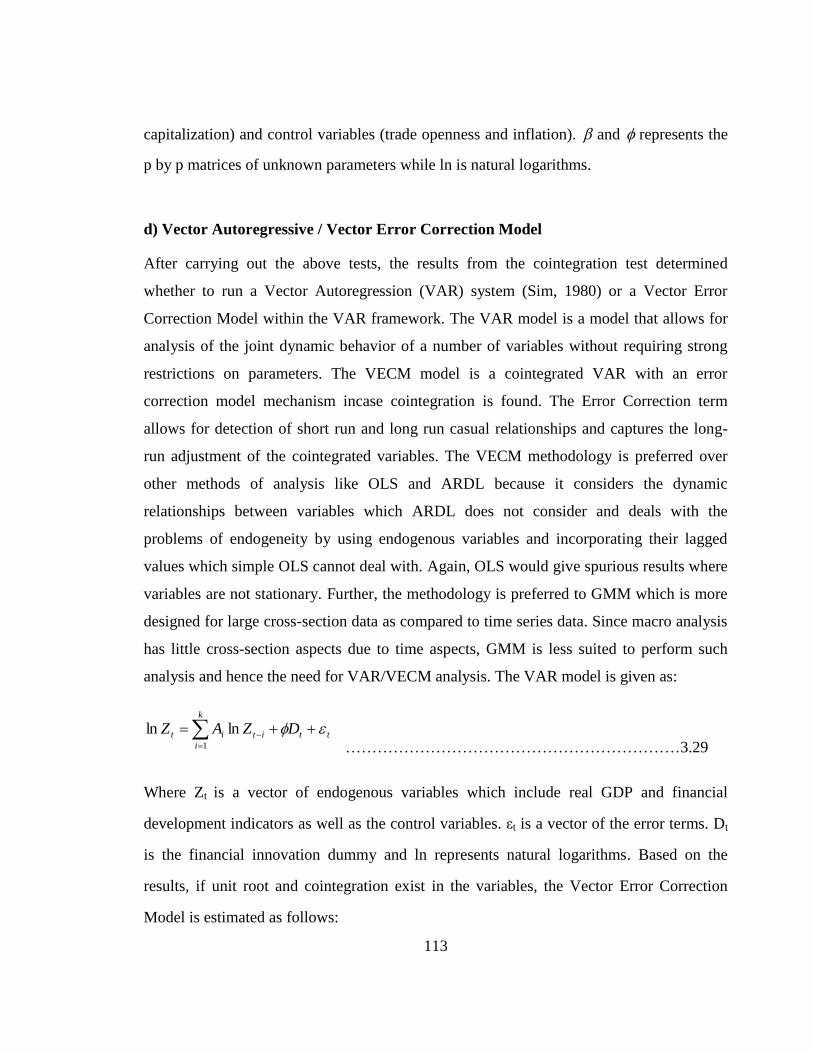
113
capitalization) and control variables (trade openness and inflation). and represents the
p by p matrices of unknown parameters while ln is natural logarithms.
d) Vector Autoregressive / Vector Error Correction Model
After carrying out the above tests, the results from the cointegration test determined
whether to run a Vector Autoregression (VAR) system (Sim, 1980) or a Vector Error
Correction Model within the VAR framework. The VAR model is a model that allows for
analysis of the joint dynamic behavior of a number of variables without requiring strong
restrictions on parameters. The VECM model is a cointegrated VAR with an error
correction model mechanism incase cointegration is found. The Error Correction term
allows for detection of short run and long run casual relationships and captures the long-
run adjustment of the cointegrated variables. The VECM methodology is preferred over
other methods of analysis like OLS and ARDL because it considers the dynamic
relationships between variables which ARDL does not consider and deals with the
problems of endogeneity by using endogenous variables and incorporating their lagged
values which simple OLS cannot deal with. Again, OLS would give spurious results where
variables are not stationary. Further, the methodology is preferred to GMM which is more
designed for large cross-section data as compared to time series data. Since macro analysis
has little cross-section aspects due to time aspects, GMM is less suited to perform such
analysis and hence the need for VAR/VECM analysis. The VAR model is given as:
tt
k
i
itit DZAZ
1
lnln
………………………………………………………3.29
Where Zt is a vector of endogenous variables which include real GDP and financial
development indicators as well as the control variables. εt is a vector of the error terms. Dt
is the financial innovation dummy and ln represents natural logarithms. Based on the
results, if unit root and cointegration exist in the variables, the Vector Error Correction
Model is estimated as follows:
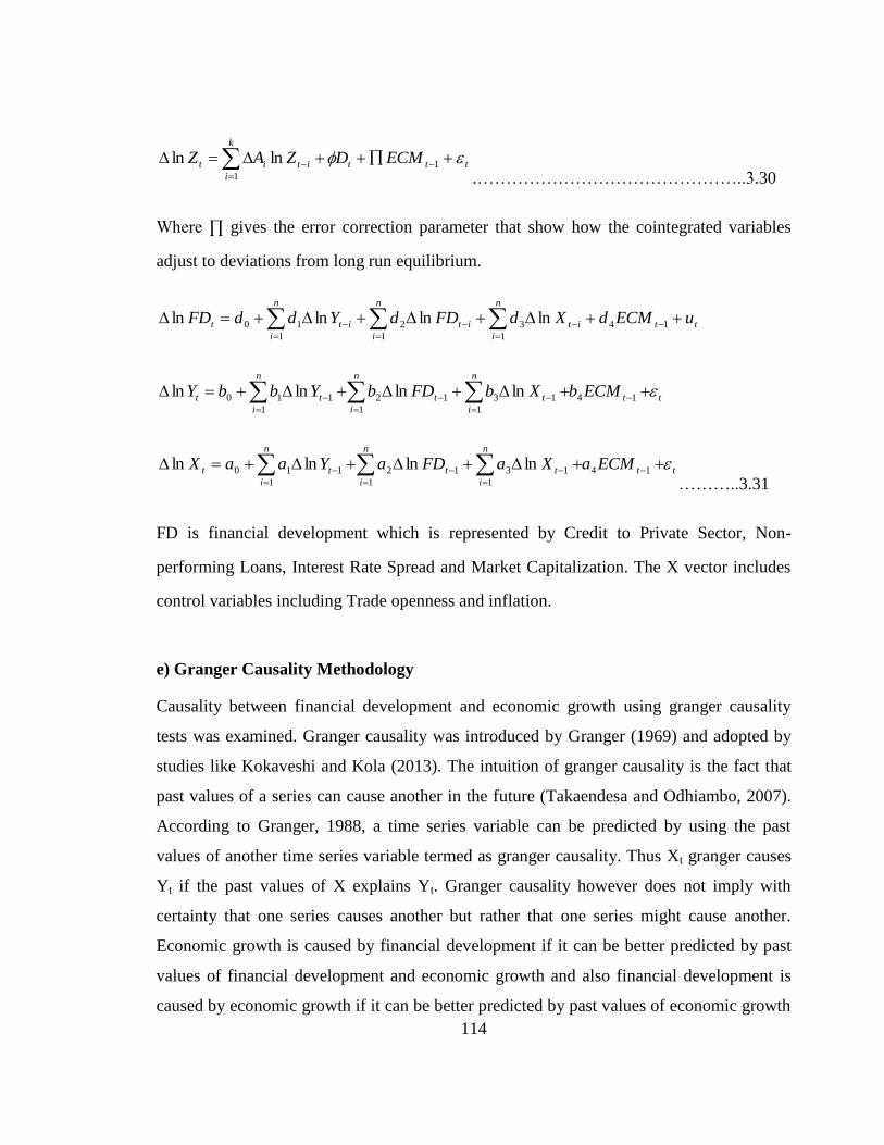
114
ttt
k
i
itit ECMDZAZ
1
1
lnln
.………………………………………..3.30
Where ∏ gives the error correction parameter that show how the cointegrated variables
adjust to deviations from long run equilibrium.
ttit
n
i
it
n
i
it
n
i
t uECMdXdFDdYddFD
14
1
3
1
2
1
10 lnlnlnln
t
n
i
t
n
i
tt
n
i
tt ECMbXbFDbYbbY
1
14
1
1312
1
110 lnlnlnln
t
n
i
t
n
i
tt
n
i
tt ECMaXaFDaYaaX
1
14
1
1312
1
110 lnlnlnln
………..3.31
FD is financial development which is represented by Credit to Private Sector, Non-
performing Loans, Interest Rate Spread and Market Capitalization. The X vector includes
control variables including Trade openness and inflation.
e) Granger Causality Methodology
Causality between financial development and economic growth using granger causality
tests was examined. Granger causality was introduced by Granger (1969) and adopted by
studies like Kokaveshi and Kola (2013). The intuition of granger causality is the fact that
past values of a series can cause another in the future (Takaendesa and Odhiambo, 2007).
According to Granger, 1988, a time series variable can be predicted by using the past
values of another time series variable termed as granger causality. Thus Xt granger causes
Yt if the past values of X explains Yt. Granger causality however does not imply with
certainty that one series causes another but rather that one series might cause another.
Economic growth is caused by financial development if it can be better predicted by past
values of financial development and economic growth and also financial development is
caused by economic growth if it can be better predicted by past values of economic growth
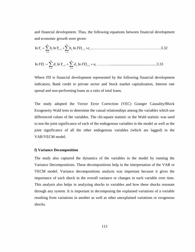
115
and financial development. Thus, the following equations between financial development
and economic growth were given:
t
n
i
t
n
i
tt FDbYbY
1
12
1
11 lnlnln ...……………………………………………..3.32
tt
n
i
t
n
i
t uFDdYdFD
1
1
21
1
1 lnlnln ………..................................................3.33
Where FD is financial development represented by the following financial development
indicators; Bank credit to private sector and Stock market capitalization, Interest rate
spread and non-performing loans as a ratio of total loans.
The study adopted the Vector Error Correction (VEC) Granger Causality/Block
Exogeneity Wald tests to determine the causal relationships among the variables which use
differenced values of the variables. The chi-square statistic or the Wald statistic was used
to test the joint significance of each of the endogenous variables in the model as well as the
joint significance of all the other endogenous variables (which are lagged) in the
VAR/VECM model.
f) Variance Decomposition
The study also captured the dynamics of the variables in the model by running the
Variance Decompositions. These decompositions help in the interpretation of the VAR or
VECM model. Variance decompositions analysis was important because it gives the
importance of each shock in the overall variance or changes in each variable over time.
This analysis also helps in analyzing shocks to variables and how these shocks resonate
through any system. It is important in decomposing the explained variations of a variable
resulting from variations in another as well as other unexplained variations or exogenous
shocks.
116
g) Post-Estimation Diagnostics
Having estimated the model, to establish the validity of the estimated results, it was
essential to conduct post estimation tests in order to ascertain the fit of the model and to
examine the structure of the residuals so as to ascertain the validity of inferences made
from the estimated results. These tests include; the model stability test, the residual
normality test, the residual autocorrelation LM test and the residual heteroscedasticity test.
3.3.4 Definition and Measurement of Variables
The variables used here represent either the allocative efficiency/productivity of capital (A)
or the proportion of savings channeled to investment, in the Pagano AK model. NPLs as
a percentage of Total loans and Bank credit to Private sector represented allocative
efficiency (A) while interest rate spread influences the proportion of savings channeled to
investment ( ) and captures transaction costs for financial intermediation. Liquid
liabilities of banks and market capitalization represented the quantity of financial
development. Liquid liabilities of banks was defined as M2 less currency in circulation,
bank credit to private sector is a measure of financial depth but isolates credit given to the
public sector. It is thus the key measure of financial intermediary development (Levine and
Zervos, 1998 and Yartey, 2007).
NPLs as a percentage of total loans is a measure of the quality of financial assets hence
quality of financial development while interest rate spread is the difference between
borrowing and lending rates by banks. It was important to include a measure of stock
market as stock markets are likely to affect the level of a country‘s economic activity by
increasing liquidity (Kenourgios and Samitas, 2007). Stock market also provides long term
finance instead of the short term finance for banks. Stock market capitalization measured
the size of the stock market and can be used as a measure of market development (Levine
and Zervos, 1998; Mohtadi and Agrawal, 1998 and Levine, 2003). Trade openness index is
defined as the sum of exports and imports of goods and services over GDP and measures a
country‘s openness to trade or integration in the world economy while inflation is the
117
overall month on month inflation and was defined as the persistent increase in the price
levels of goods and services over a certain time period. It captures the extent of future
uncertainty which makes firms shy away from making long term investment decisions due
to high price volatility (Caporale et al., 2009). Real Gross Domestic Product is used as a
proxy for economic growth.
Financial innovation is represented by the volumes of money transacted through mobile
money in specific M-Pesa. However, since the data observations for mobile payments were
few (from 2007) and would not allow for enough degrees of freedom, a dummy variable
was used to represent onset of M-Pesa accompanied with M-Pesa volumes of transactions.
The dummy was one from quarter two of 2007 onwards when mobile payments through
M-Pesa started and zero otherwise.
In regards to economic growth, it is noted that growth of GDP is mostly used in cross-
sectional and panel data analysis since countries do not have similar aggregate production
functions and comparisons using growth would be ideal (Greiner et al., 2004) although it
has been used in time series studies (Dushku, 2010 and Shan and Jianhong, 2006, ). In this
study, real GDP is used as a measure of economic growth as used in literature (Jalil and
Feridun, 2011; Kargbo and Adamu, 2010; Mittal, 2014 and Ghatak and Siddiki, 1999).
Further, introducing logarithms ensures that the log difference of real GDP gives economic
growth (Herzer and Morrissey, 2011; Kargbo and Adamu, 2010 and Kargbo, 2012). Table
3.2 summarises the definition and measurement of variables.

118
Table 3.2: Definition and Measurement of Variables
Variable Definition and Measurement Expected
Sign
Literature Source Unit of
Measurement
Real GDP (GDP) It gives the value of all goods and
services produced in a country in a
year expressed in 2009 prices taking
inflation into consideration
Kargbo and Adamu
(2010), Mittal (2014)
Kshs.
Credit to Private
Sector (CPS)
This is the credit/loans offered by the
banking industry to the private
sector.
Positive Levine and Zervos
(1998), Yartey
(2007), Liang and
Teng(2006),
Adamopoulos (2010),
Arcand et al. (2011)
Kshs.
Liquid Liabilities of
Banks (LL)
This is the defined as broad money,
M2 less currency outside banks or
currency in circulation.
Positive De Gregorio and
Guidotti (1995),
Dushku (2010)
Kshs.
Market
Capitalization
(MKT)
It is the value of all outstanding
shares of all companies listed at the
Nairobi Stock exchange. It is
calculated by multiplying all the
outstanding shares by their current
market prices.
Positive Kenourgios and
Samitas, 2007,
Levine and Zervos
(1998), Mohtadi and
Agrawal (1998) and
Levine (2003
Kshs.
Non - Performing
Loans (NPL)
The sum of loans for which the
borrowers have not made payment
for atleast 90 days. It is measured as
the value of NPLs divided by the
total value of the loan portfolio. It is
a measure of the quality of financial
development
Negative Dudian and Popa
(2013)
Ratio
Interest Rate Spread
(INT)
It is the difference between
borrowing (demand, time and
savings deposits) and lending (loans)
rates by banks. It measures the
efficiency of the banking sector
Negative Antzoulatos et al
(2008), Dudian
(2013)
Rate
Financial
Innovation (FI)
This is represented by a dummy
variable. The dummy is one from
quarter two of 2007 onwards when
M-Pesa was introduced and zero
otherwise.
Positive This measure is new
literature and it is
justified in (Krishnan,
2011)
Dummy
Inflation (INF) Overall month on month inflation
and is defined as the continuous
increment in price levels of goods
and services over a certain time
period. The month on month values
are then added per quarter and
divided by 3
Negative Easterly and Fischer
(2001), Dollar and
Kraay (2002) and
Rate
Trade Openness
(TO)
Sum of exports and imports of goods
and services over GDP and it
measures a country‘s openness to
trade or integration in the world
economy
Positive Wolde-Rufael (2009)
and Menyah et. al
(2014)
Index
119
All the variables were in logarithm form as described in section 2.3.3 in chapter 2 apart
from the financial innovation dummy. The study uses LN to represent natural logarithm.
3.3.5 Data Set and Description
Quarterly time series data, which cover the 2000 to 2014 period, was utilized in this study.
The choice of this period was due to the availability of quarterly data which stems from the
year 2000. The study differs from other studies especially the ones done in Kenya by using
quarterly frequency data. Less developed countries like Kenya rarely have data that covers
long span of time. Quarterly data comes in handy in this situation and larger data
observations can help in attaining more statistically significant estimates. Putsis (1996)
also concluded that use of quarterly data can lead to more accurate forecasts than annual
data. The data was largely obtained from the CBK annual, quarterly and monthly reports
from the years 2000 to 2014. In addition, the stock market data was collected from NSE.
Data on GDP was obtained from the Kenya National Bureau of Statistics (KNBS),
quarterly statistical reports.
3.4 Empirical Results and Discussion
3.4.1 Descriptive Statistics
The study determined the spread of the data giving both the mean and the standard
deviation to show the deviations from the mean. The study also tested for normality of the
variables using the JB test which compares the skewness and kurtosis coefficients of the
variables. These results are as discussed in Table 2.2 in section 2.4 in chapter 2. All the
variables were not highly dispersed from their mean values as shown by their small
standard deviations. From the values of skewness and kurtosis and the Jarque – Bera
probability, real GDP, market capitalization, trade openness and inflation were normally
distributed at five percent significance level. However, at one percent significance level, all
the variables were normally distributed. This was important as it shows how reliable data is
in the results and in this case, then the data was reliable.
120
3.4.2 Correlation Matrix
Correlation shows the linear relationship between variables. It interrogates the relationship
between pairs of variables. High pairwise correlations imply multicollinearity problems
which could lead to high standard errors and insignificant statistics, thus inaccuracy of the
regression coefficients. There was high correlation (0.87) between credit to private sector
and liquid liabilities of banks as shown in Table A.3 (Appendix). Correlations above 0.70
are considered to be high (Fawcett, 2007). High pairwise correlations indicate
multicollinearity problems and hence the t statistics and regression coefficients cannot be
trusted. So the study dropped liquid liabilities of banks and used Credit to private sector
because it shows the financial depth as compared to liquid liabilities of banks which shows
more of the liquidity aspect. All the other variables were not highly correlated but both
positive and negative correlations were evident between the various variables.
3.4.3 Unit Root Tests
It was important to determine the optimal lag length of each variable. This is important in
testing for unit root as ignoring this could lead to giving the false stationarity results. The
tests for optimal lag length which were conducted included Fixed Prediction Error (FPE),
Akaike Information Criteria (AIC), Hannan and Quinn Information Criteria (HQIC) and
Schwarz‘ Bayesian Information Criteria (SBIC). For almost all the variables, all the lag
length tests determined the same lag length as shown in Table A.1 (Appendix). Credit to
Private Sector, Non-perfoming Loans, trade openness and remittances had an optimal lag
length of three, market capitalization and real gdp had a lag length of one while inflation
had a lag length of four.
A graphical presentation of the variables was important so as to capture their movement
over time. This was important because it shows whether the variables had a deterministic
trend or not. This gives guidance on whether to include a trend and intercept or not when
conducting stationarity tests. These graphs are indicated in Appendix. From the graph, it
was clear that all the variables had a trend.The stationarity properties of the variables were

121
determined by conducting unit root tests. This was important as ignoring stationarity
properties would lead to spurious regression. The study conducted the Phillip - Perron unit
root test and the results are given in Table 3.3:
Table 3.3: Phillip - Perron Unit Root Test Results
At levels 1st difference Order of
integrati
on Constant Trend &
Intercept
Constant Trend &
Intercept
Variables t-stat 5%
Critical
value
t-stat 5%
Critica
l value
t-stat 5%
Critica
l value
t-stat 5%
Critica
l value
LNReal GDP 1.057 -2.916 -2.049 -3.495 -4.217 -2.916 -11.947 -3.494 1(1) LNCredit to
Private Sector 1.134 -2.917 -3.142 -3.497 -2.632 -2.596 -3.296 -3.177 1(1)
LNMarket
Capitalization -0.527 -2.912 -1.420 -3.489 -6.355 -2.912 -6.289 -3.489 1(1)
LNNon-
performing
Loans
-0.644 -2.912 -1.711 -3.489 -6.936 -2.913 -6.875 -3.491 1(1)
LNInflation -3.048 -2.916 -3.153 -3.495 -6.231 -2.916 -6.235 -3.494 1(1) LNInterest Rate
Spread -1.213 -2.912 -1.397 -3.488 -6.733 -2.912 -6.673 -3.489 1(1)
LNTrade
Openness -1.750 -2.912 -3.492 -3.495 -7.602 -2.914 -7.594 -3.492 1(1)
Results from the Phillip – Perron test showed that, all the variables are integrated of order
one meaning that they were non-stationary at levels but stationary at first difference.
The study conducted Zivot-Andrews unit root test to test for unit root in the presence of
structural breaks. The test combines both intercept and trend in testing for unit root in the
presence of a structural break. From the results of the Zivot-Andrews test as summarized in
Table 3.4, all variables were integrated of order one.
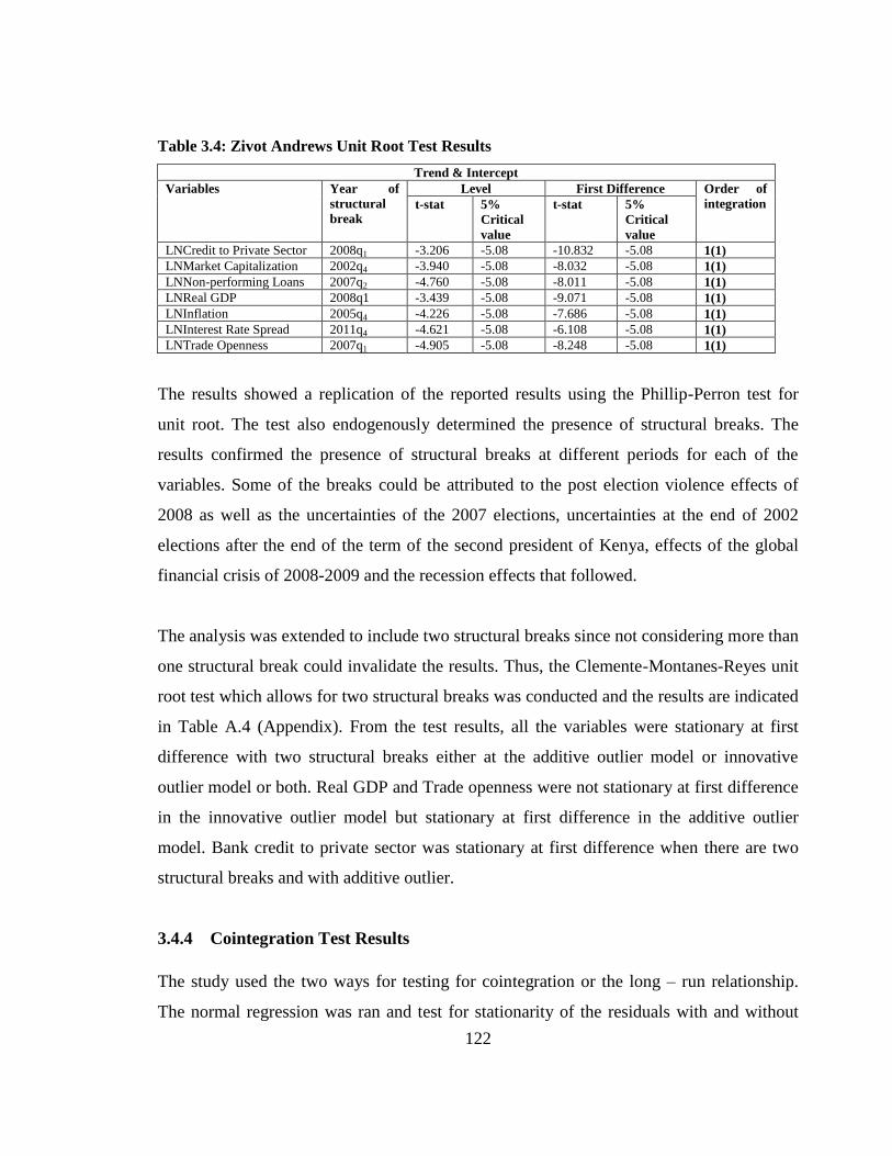
122
Table 3.4: Zivot Andrews Unit Root Test Results
Trend & Intercept
Variables Year of
structural
break
Level First Difference Order of
integration t-stat 5%
Critical
value
t-stat 5%
Critical
value
LNCredit to Private Sector 2008q1 -3.206 -5.08 -10.832 -5.08 1(1)
LNMarket Capitalization 2002q4 -3.940 -5.08 -8.032 -5.08 1(1)
LNNon-performing Loans 2007q2 -4.760 -5.08 -8.011 -5.08 1(1)
LNReal GDP 2008q1 -3.439 -5.08 -9.071 -5.08 1(1)
LNInflation 2005q4 -4.226 -5.08 -7.686 -5.08 1(1)
LNInterest Rate Spread 2011q4 -4.621 -5.08 -6.108 -5.08 1(1)
LNTrade Openness 2007q1 -4.905 -5.08 -8.248 -5.08 1(1)
The results showed a replication of the reported results using the Phillip-Perron test for
unit root. The test also endogenously determined the presence of structural breaks. The
results confirmed the presence of structural breaks at different periods for each of the
variables. Some of the breaks could be attributed to the post election violence effects of
2008 as well as the uncertainties of the 2007 elections, uncertainties at the end of 2002
elections after the end of the term of the second president of Kenya, effects of the global
financial crisis of 2008-2009 and the recession effects that followed.
The analysis was extended to include two structural breaks since not considering more than
one structural break could invalidate the results. Thus, the Clemente-Montanes-Reyes unit
root test which allows for two structural breaks was conducted and the results are indicated
in Table A.4 (Appendix). From the test results, all the variables were stationary at first
difference with two structural breaks either at the additive outlier model or innovative
outlier model or both. Real GDP and Trade openness were not stationary at first difference
in the innovative outlier model but stationary at first difference in the additive outlier
model. Bank credit to private sector was stationary at first difference when there are two
structural breaks and with additive outlier.
3.4.4 Cointegration Test Results
The study used the two ways for testing for cointegration or the long – run relationship.
The normal regression was ran and test for stationarity of the residuals with and without
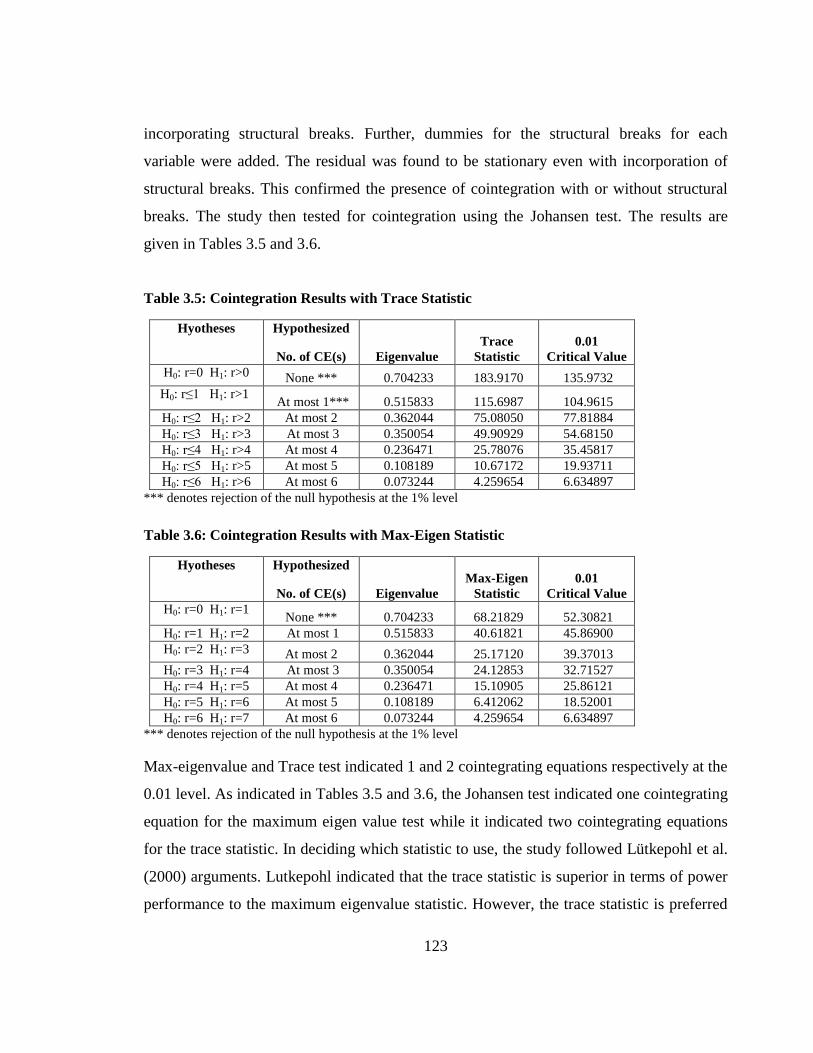
123
incorporating structural breaks. Further, dummies for the structural breaks for each
variable were added. The residual was found to be stationary even with incorporation of
structural breaks. This confirmed the presence of cointegration with or without structural
breaks. The study then tested for cointegration using the Johansen test. The results are
given in Tables 3.5 and 3.6.
Table 3.5: Cointegration Results with Trace Statistic
Hyotheses Hypothesized
No. of CE(s) Eigenvalue
Trace
Statistic
0.01
Critical Value
H0: r=0 H1: r>0 None *** 0.704233 183.9170 135.9732
H0: r≤1 H1: r>1 At most 1*** 0.515833 115.6987 104.9615
H0: r≤2 H1: r>2 At most 2 0.362044 75.08050 77.81884
H0: r≤3 H1: r>3 At most 3 0.350054 49.90929 54.68150
H0: r≤4 H1: r>4 At most 4 0.236471 25.78076 35.45817
H0: r≤5 H1: r>5 At most 5 0.108189 10.67172 19.93711
H0: r≤6 H1: r>6 At most 6 0.073244 4.259654 6.634897
*** denotes rejection of the null hypothesis at the 1% level
Table 3.6: Cointegration Results with Max-Eigen Statistic
Hyotheses Hypothesized
No. of CE(s) Eigenvalue
Max-Eigen
Statistic
0.01
Critical Value
H0: r=0 H1: r=1 None *** 0.704233 68.21829 52.30821
H0: r=1 H1: r=2 At most 1 0.515833 40.61821 45.86900
H0: r=2 H1: r=3 At most 2 0.362044 25.17120 39.37013
H0: r=3 H1: r=4 At most 3 0.350054 24.12853 32.71527
H0: r=4 H1: r=5 At most 4 0.236471 15.10905 25.86121
H0: r=5 H1: r=6 At most 5 0.108189 6.412062 18.52001
H0: r=6 H1: r=7 At most 6 0.073244 4.259654 6.634897
*** denotes rejection of the null hypothesis at the 1% level
Max-eigenvalue and Trace test indicated 1 and 2 cointegrating equations respectively at the
0.01 level. As indicated in Tables 3.5 and 3.6, the Johansen test indicated one cointegrating
equation for the maximum eigen value test while it indicated two cointegrating equations
for the trace statistic. In deciding which statistic to use, the study followed Lütkepohl et al.
(2000) arguments. Lutkepohl indicated that the trace statistic is superior in terms of power
performance to the maximum eigenvalue statistic. However, the trace statistic is preferred
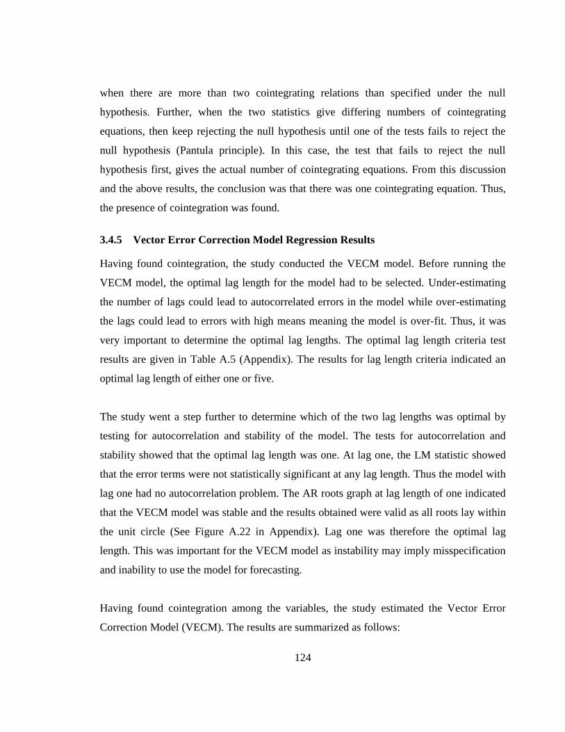
124
when there are more than two cointegrating relations than specified under the null
hypothesis. Further, when the two statistics give differing numbers of cointegrating
equations, then keep rejecting the null hypothesis until one of the tests fails to reject the
null hypothesis (Pantula principle). In this case, the test that fails to reject the null
hypothesis first, gives the actual number of cointegrating equations. From this discussion
and the above results, the conclusion was that there was one cointegrating equation. Thus,
the presence of cointegration was found.
3.4.5 Vector Error Correction Model Regression Results
Having found cointegration, the study conducted the VECM model. Before running the
VECM model, the optimal lag length for the model had to be selected. Under-estimating
the number of lags could lead to autocorrelated errors in the model while over-estimating
the lags could lead to errors with high means meaning the model is over-fit. Thus, it was
very important to determine the optimal lag lengths. The optimal lag length criteria test
results are given in Table A.5 (Appendix). The results for lag length criteria indicated an
optimal lag length of either one or five.
The study went a step further to determine which of the two lag lengths was optimal by
testing for autocorrelation and stability of the model. The tests for autocorrelation and
stability showed that the optimal lag length was one. At lag one, the LM statistic showed
that the error terms were not statistically significant at any lag length. Thus the model with
lag one had no autocorrelation problem. The AR roots graph at lag length of one indicated
that the VECM model was stable and the results obtained were valid as all roots lay within
the unit circle (See Figure A.22 in Appendix). Lag one was therefore the optimal lag
length. This was important for the VECM model as instability may imply misspecification
and inability to use the model for forecasting.
Having found cointegration among the variables, the study estimated the Vector Error
Correction Model (VECM). The results are summarized as follows:
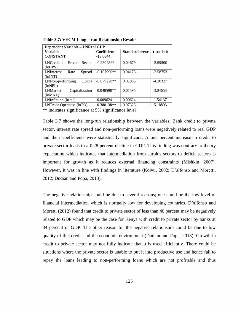
125
Table 3.7: VECM Long – run Relationship Results
Dependent Variable – LNReal GDP
Variable Coefficient Standard error t-statistic
CONSTANT -13.0844
LNCredit to Private Sector
(lnCPS)
-0.28048** 0.04679 -5.99500
LNInterest Rate Spread
(lnINT)
-0.107990** 0.04173 -2.58753
LNNon-performing Loans
(lnNPL)
-0.079228** 0.01885 -4.20327
LNMarket Capitalization
(lnMKT)
0.048598** 0.01595 3.04653
LNInflation (ln ) 0.009624 0.00624 1.54137
LNTrade Openness (lnTO) 0.380138** 0.07326 5.18893
** indicates significance at 5% significance level
Table 3.7 shows the long-run relationship between the variables. Bank credit to private
sector, interest rate spread and non-performing loans were negatively related to real GDP
and their coefficients were statistically significant. A one percent increase in credit to
private sector leads to a 0.28 percent decline in GDP. This finding was contrary to theory
expectation which indicates that intermediation from surplus sectors to deficit sectors is
important for growth as it reduces external financing constraints (Mishkin, 2007).
However, it was in line with findings in literature (Koivu, 2002; D‘alfonso and Moretti,
2012; Dudian and Popa, 2013).
The negative relationship could be due to several reasons; one could be the low level of
financial intermediation which is normally low for developing countries. D‘alfonso and
Moretti (2012) found that credit to private sector of less than 40 percent may be negatively
related to GDP which may be the case for Kenya with credit to private sector by banks at
34 percent of GDP. The other reason for the negative relationship could be due to low
quality of this credit and the economic environment (Dudian and Popa, 2013). Growth in
credit to private sector may not fully indicate that it is used efficiently. There could be
situations where the private sector is unable to put it into productive use and hence fail to
repay the loans leading to non-performing loans which are not profitable and thus
126
reductions in further credit hence reduction in economic performance. In some countries,
this has led to banking crises.
The coefficient of interest rate spread was significant and indicated that a one percent
increase in interest rate spread leads to 0.11 percent decline in GDP. The higher the interest
rate spread, the lower the affordability of credit and thus less investments. This happens
when the spread is caused by an increase in lending rate, holding the deposit rate constant,
lowering it or increasing it at a lower rate than the lending rate. This is the case in Kenya,
where the interest rate spread is high because banks have previously maintained very low
deposit rates while charging very high borrowing rates. The interest rate spread is a
measure of transaction costs as well as efficiency and the negative sign was consistent with
theory (Harrison et al., 1999) which indicated that a lower interest rate spread or margin
encourages investment and thus spurs economic growth. High interest rate spread is also
asymptomatic of other imperfections in the financial sector and hence may undermine
growth. Bank credit to private sector may only show the size of the financial sector but not
the quality of the sector. To show the quality of the financial sector, non-performing loans
was used.
The results showed that, an increase in non-performing loans led to reduction in real GDP.
The coefficient was significant and indicated that a one percent increase in non-performing
loans led to 0.08 percent reduction in GDP. This was as supported by theory which
indicates that inefficiency of the financial sector leads to inefficient allocation of resources
(Bencivenga and Smith, 1991) and non-performing loans may lead to a credit crunch
(Krueger and Tornell, 1999). Non-performing loans may cause financial institutions to be
burdened with large loans of negative real value thus reducing their ability to give new
loans for investment and thus reduced economic performance. NPLs may also indicate that
banks are financing non-productive or political activities which have a dampening effect
on economic growth. They may also result from high interest rates that attract high risk
borrowers engaged in activities not conducive to growth.
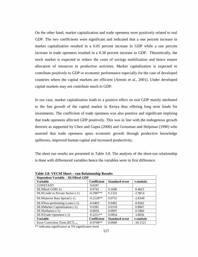
127
On the other hand, market capitalization and trade openness were positively related to real
GDP. The two coefficients were significant and indicated that a one percent increase in
market capitalization resulted in a 0.05 percent increase in GDP while a one percent
increase in trade openness resulted in a 0.38 percent increase in GDP. Theoretically, the
stock market is expected to reduce the costs of savings mobilization and hence ensure
allocation of resources to productive activities. Market capitalization is expected to
contribute positively to GDP or economic performance especially for the case of developed
countries where the capital markets are efficient (Arestis et al., 2001). Under developed
capital markets may not contribute much to GDP.
In our case, market capitalization leads to a positive effect on real GDP mainly attributed
to the fast growth of the capital market in Kenya thus offering long term funds for
investments. The coefficient of trade openness was also positive and significant implying
that trade openness affected GDP positively. This was in line with the endogenous growth
theories as supported by Chen and Gupta (2006) and Grossman and Helpman (1990) who
asserted that trade openness spurs economic growth through productive knowledge
spillovers, improved human capital and increased productivity.
The short run results are presented in Table 3.8. The analysis of the short-run relationship
is done with differenced variables hence the variables were in first difference.
Table 3.8: VECM Short – run Relationship Results Dependent Variable – DLNReal GDP
Variable Coefficient Standard error t-statistic
CONSTANT 0.0187
DLNReal GDP(-1) 0.0742 0.1606 0.4623
DLNCredit to Private Sector (-1) -0.3987** 0.1333 -2.9914
DLNInterest Rate Spread (-1) -0.2128** 0.0751 -2.8349
DLNNon-performing Loans (-1) -0.0403 0.0482 -0.8361
DLNMarket Capitalization (-1) 0.0281 0.0318 0.8847
DLNInflation (-1) 0.0058 0.0097 0.5960
DLNTrade Openness (-1) 0.3251** 0.0854 3.8056
Variable Coefficient Standard error t-statistic
Error Correction Term (ECTt-1) -0.9708** 0.0960 -10.1121
** indicates significance at 5% significance level
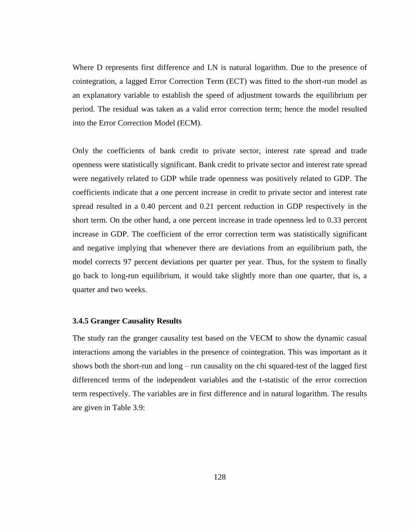
128
Where D represents first difference and LN is natural logarithm. Due to the presence of
cointegration, a lagged Error Correction Term (ECT) was fitted to the short-run model as
an explanatory variable to establish the speed of adjustment towards the equilibrium per
period. The residual was taken as a valid error correction term; hence the model resulted
into the Error Correction Model (ECM).
Only the coefficients of bank credit to private sector, interest rate spread and trade
openness were statistically significant. Bank credit to private sector and interest rate spread
were negatively related to GDP while trade openness was positively related to GDP. The
coefficients indicate that a one percent increase in credit to private sector and interest rate
spread resulted in a 0.40 percent and 0.21 percent reduction in GDP respectively in the
short term. On the other hand, a one percent increase in trade openness led to 0.33 percent
increase in GDP. The coefficient of the error correction term was statistically significant
and negative implying that whenever there are deviations from an equilibrium path, the
model corrects 97 percent deviations per quarter per year. Thus, for the system to finally
go back to long-run equilibrium, it would take slightly more than one quarter, that is, a
quarter and two weeks.
3.4.5 Granger Causality Results
The study ran the granger causality test based on the VECM to show the dynamic casual
interactions among the variables in the presence of cointegration. This was important as it
shows both the short-run and long – run causality on the chi squared-test of the lagged first
differenced terms of the independent variables and the t-statistic of the error correction
term respectively. The variables are in first difference and in natural logarithm. The results
are given in Table 3.9:
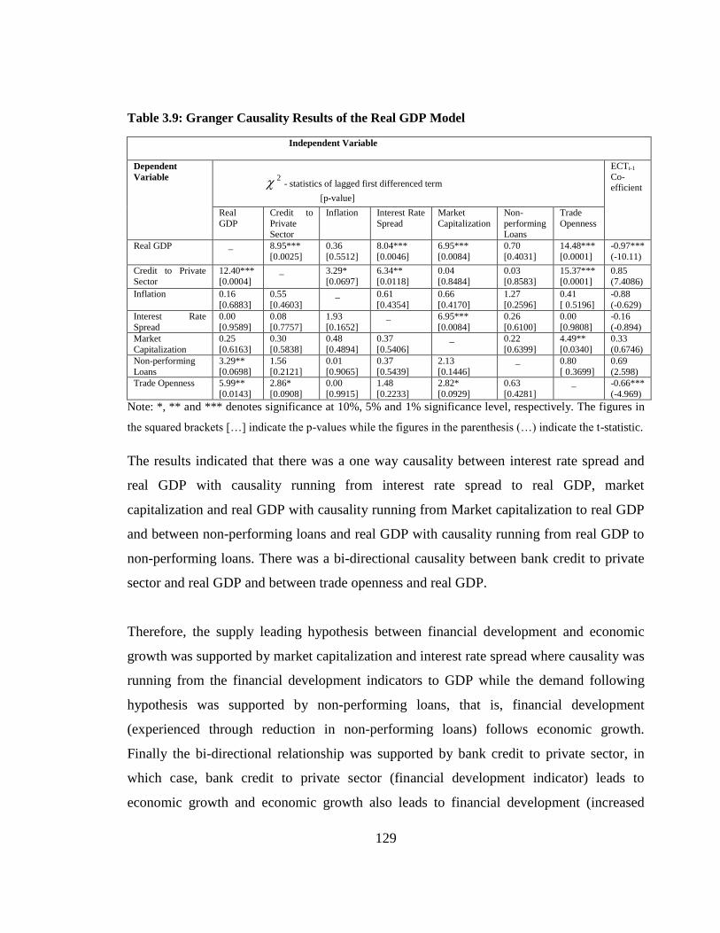
129
Table 3.9: Granger Causality Results of the Real GDP Model
Independent Variable
Dependent
Variable
2 - statistics of lagged first differenced term
[p-value]
ECTt-1
Co-efficient
Real
GDP
Credit to
Private Sector
Inflation Interest Rate
Spread
Market
Capitalization
Non-
performing Loans
Trade
Openness
Real GDP _ 8.95***
[0.0025]
0.36
[0.5512]
8.04***
[0.0046]
6.95***
[0.0084]
0.70
[0.4031]
14.48***
[0.0001]
-0.97***
(-10.11)
Credit to Private
Sector
12.40***
[0.0004]
_ 3.29*
[0.0697]
6.34**
[0.0118]
0.04
[0.8484]
0.03
[0.8583]
15.37***
[0.0001]
0.85
(7.4086)
Inflation 0.16
[0.6883]
0.55
[0.4603]
_ 0.61
[0.4354]
0.66
[0.4170]
1.27
[0.2596]
0.41
[ 0.5196]
-0.88
(-0.629)
Interest Rate
Spread
0.00
[0.9589]
0.08
[0.7757]
1.93
[0.1652]
_ 6.95***
[0.0084]
0.26
[0.6100]
0.00
[0.9808]
-0.16
(-0.894)
Market
Capitalization
0.25
[0.6163]
0.30
[0.5838]
0.48
[0.4894]
0.37
[0.5406]
_ 0.22
[0.6399]
4.49**
[0.0340]
0.33
(0.6746)
Non-performing
Loans
3.29**
[0.0698]
1.56
[0.2121]
0.01
[0.9065]
0.37
[0.5439]
2.13
[0.1446]
_ 0.80
[ 0.3699]
0.69
(2.598)
Trade Openness 5.99**
[0.0143]
2.86*
[0.0908]
0.00
[0.9915]
1.48
[0.2233]
2.82*
[0.0929]
0.63
[0.4281]
_ -0.66***
(-4.969)
Note: *, ** and *** denotes significance at 10%, 5% and 1% significance level, respectively. The figures in
the squared brackets […] indicate the p-values while the figures in the parenthesis (…) indicate the t-statistic.
The results indicated that there was a one way causality between interest rate spread and
real GDP with causality running from interest rate spread to real GDP, market
capitalization and real GDP with causality running from Market capitalization to real GDP
and between non-performing loans and real GDP with causality running from real GDP to
non-performing loans. There was a bi-directional causality between bank credit to private
sector and real GDP and between trade openness and real GDP.
Therefore, the supply leading hypothesis between financial development and economic
growth was supported by market capitalization and interest rate spread where causality was
running from the financial development indicators to GDP while the demand following
hypothesis was supported by non-performing loans, that is, financial development
(experienced through reduction in non-performing loans) follows economic growth.
Finally the bi-directional relationship was supported by bank credit to private sector, in
which case, bank credit to private sector (financial development indicator) leads to
economic growth and economic growth also leads to financial development (increased
130
bank loans to private sector). The channels between the dependent and independent
variables with emphasis on the financial development indicators were summarised in
Figure 3.2:
Figure 3.2: Causality between Real GDP and Financial Development Indicators
Source: Author‘s compilation from the empirical results
3.4.6 Variance Decomposition
The study ran the VECM model which indicates the exogeinity and endogeinity of the
variables in the system and the granger causality based on the VECM model to determine
the causality between the financial development indicators and real GDP. The study
further sought to determine the dynamic properties or interactions of the variables within a
system using the variance decompositions. The variance decomposition method used was
the cholesky decomposition. This method is preferred because the other non-orthogonal
factorization methods, shocks to one unit, shocks to one standard deviation do not fufill the
adding up property. The rows show the forecast variance percentage due to each shock and
should add up to 100. The results are presented in Tables 3.10 and 3.11.
Demand following hypothesis
Supply leading hypothesis
Supply leading hypothesis
Bi-directional relationship Credit to Private
Sector
Market
Capitalization
Interest Rate
Spread
Non-performing
Loans
GDP
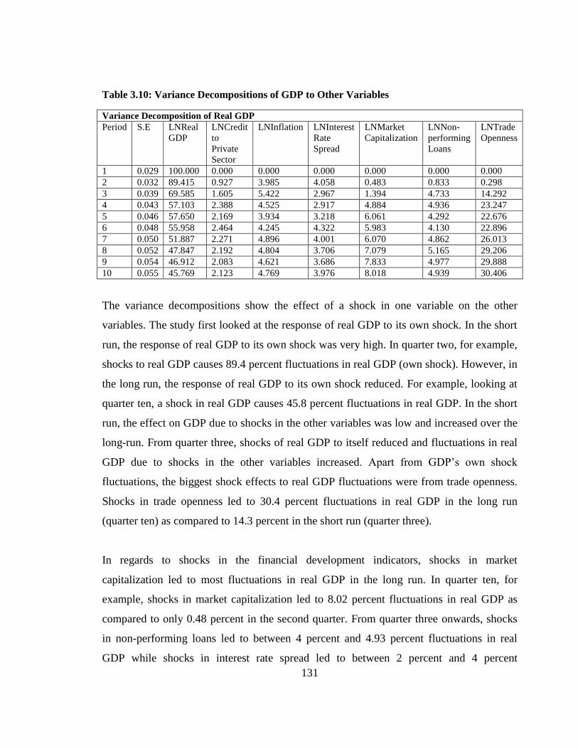
131
Table 3.10: Variance Decompositions of GDP to Other Variables
Variance Decomposition of Real GDP
Period S.E LNReal
GDP
LNCredit
to
Private
Sector
LNInflation LNInterest
Rate
Spread
LNMarket
Capitalization
LNNon-
performing
Loans
LNTrade
Openness
1 0.029 100.000 0.000 0.000 0.000 0.000 0.000 0.000
2 0.032 89.415 0.927 3.985 4.058 0.483 0.833 0.298
3 0.039 69.585 1.605 5.422 2.967 1.394 4.733 14.292
4 0.043 57.103 2.388 4.525 2.917 4.884 4.936 23.247
5 0.046 57.650 2.169 3.934 3.218 6.061 4.292 22.676
6 0.048 55.958 2.464 4.245 4.322 5.983 4.130 22.896
7 0.050 51.887 2.271 4.896 4.001 6.070 4.862 26.013
8 0.052 47.847 2.192 4.804 3.706 7.079 5.165 29.206
9 0.054 46.912 2.083 4.621 3.686 7.833 4.977 29.888
10 0.055 45.769 2.123 4.769 3.976 8.018 4.939 30.406
The variance decompositions show the effect of a shock in one variable on the other
variables. The study first looked at the response of real GDP to its own shock. In the short
run, the response of real GDP to its own shock was very high. In quarter two, for example,
shocks to real GDP causes 89.4 percent fluctuations in real GDP (own shock). However, in
the long run, the response of real GDP to its own shock reduced. For example, looking at
quarter ten, a shock in real GDP causes 45.8 percent fluctuations in real GDP. In the short
run, the effect on GDP due to shocks in the other variables was low and increased over the
long-run. From quarter three, shocks of real GDP to itself reduced and fluctuations in real
GDP due to shocks in the other variables increased. Apart from GDP‘s own shock
fluctuations, the biggest shock effects to real GDP fluctuations were from trade openness.
Shocks in trade openness led to 30.4 percent fluctuations in real GDP in the long run
(quarter ten) as compared to 14.3 percent in the short run (quarter three).
In regards to shocks in the financial development indicators, shocks in market
capitalization led to most fluctuations in real GDP in the long run. In quarter ten, for
example, shocks in market capitalization led to 8.02 percent fluctuations in real GDP as
compared to only 0.48 percent in the second quarter. From quarter three onwards, shocks
in non-performing loans led to between 4 percent and 4.93 percent fluctuations in real
GDP while shocks in interest rate spread led to between 2 percent and 4 percent

132
fluctuations in real GDP. Shocks in bank credit to private sector led to the least
fluctuations in real GDP of upto 2.46 percent in the sixth quarter.
The reason why shocks to market capitalization would have a longer lasting effect on
national income than the other financial development indicators would be the theoretical
underpinnings that stock markets usually provide long-term funds for investment. These
long-term funds would be key for long term growth due to increased investment (Arestis et
al., 2001). Well performing stock markets reduce the cost of savings mobilization and
ensure productive allocation of resources. Kenya‘s capital market has been growing
speedily and is currently the second largest in Africa after South Africa‘s in terms of
market capitalization (World Bank, 2013b).
Table 3.11: Variance Decomposition of Other Variables to GDP
Variance Decomposition of other variables to GDP
Period S.E LNReal
GDP
LNCredit to
Private Sector
LNInflation LNInterest
Rate Spread
LNMarket
Capitalization
1 74.628 8.399 0.005 35.004 0.178 0.274
2 37.297 9.634 0.594 32.454 0.671 7.619
3 23.321 10.032 0.501 28.874 2.075 18.383
4 16.555 10.067 0.438 26.939 2.005 18.814
5 15.824 9.8196 0.446 26.616 1.698 17.433
6 13.235 9.725 0.449 26.377 1.712 18.233
7 10.756 9.784 0.409 25.667 1.945 20.214
8 9.509 9.799 0.369 25.037 1.987 20.629
9 9.305 9.737 0.349 24.778 1.919 20.300
10 8.826 9.693 0.337 24.609 1.918 20.488
Shocks in real GDP led to increasing fluctuations in trade openness, increasing from 0.3
percent in quarter one to 20.5 percent in quarter eight. Fluctuations in inflation in response
to shocks in real GDP were constant at 8 to 10 percent. As for the financial development
indicators, shocks in real GDP led to higher fluctuations in bank credit to private sector in
the short run. However, these fluctuations reduced in the long run standing at 8.8 percent
in quarter ten as compared to 74.6 percent in the short run (quarter one). 35 percent
fluctuations in market capitalization in quarter one was due to shocks in real GDP which
reduced to 24.6 percent in quarter ten. Shocks in real GDP did not lead to large
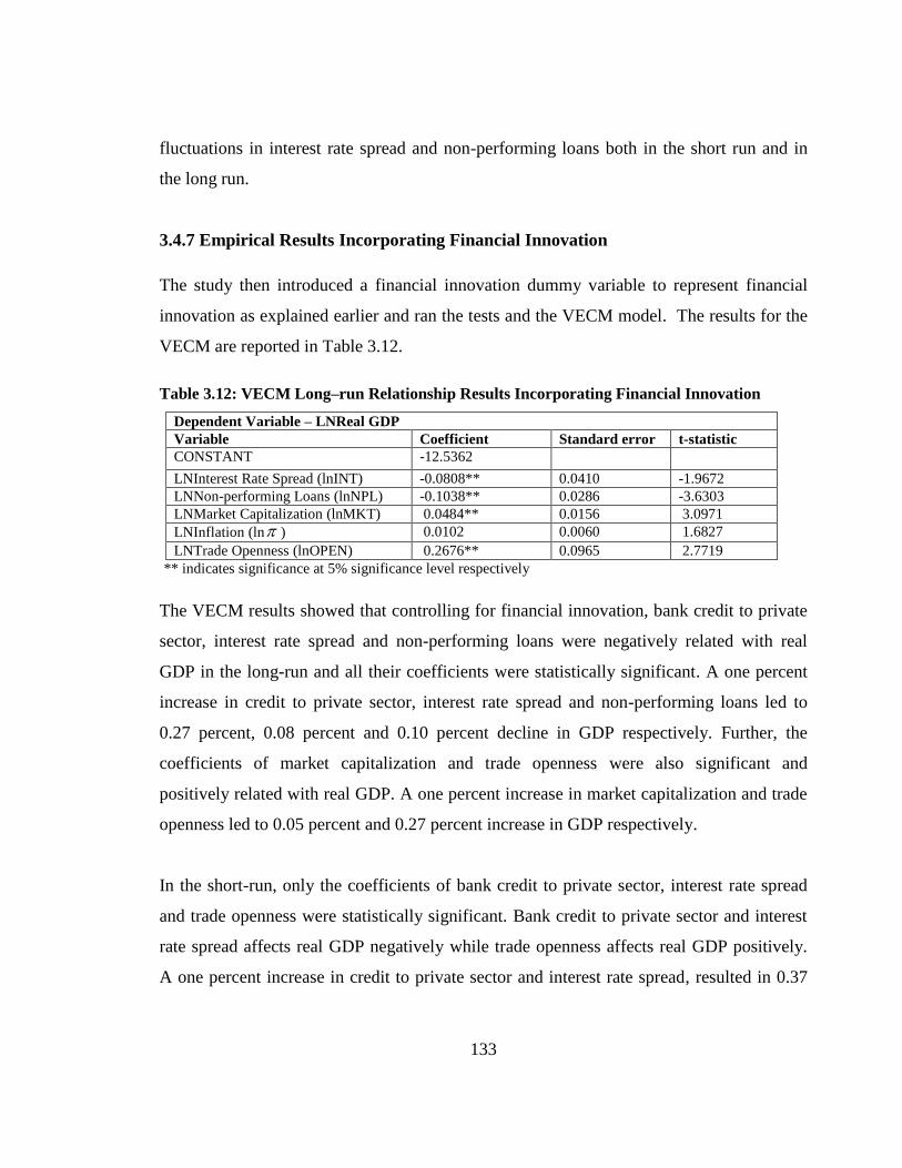
133
fluctuations in interest rate spread and non-performing loans both in the short run and in
the long run.
3.4.7 Empirical Results Incorporating Financial Innovation
The study then introduced a financial innovation dummy variable to represent financial
innovation as explained earlier and ran the tests and the VECM model. The results for the
VECM are reported in Table 3.12.
Table 3.12: VECM Long–run Relationship Results Incorporating Financial Innovation
Dependent Variable – LNReal GDP
Variable Coefficient Standard error t-statistic
CONSTANT -12.5362
LNInterest Rate Spread (lnINT) -0.0808** 0.0410 -1.9672
LNNon-performing Loans (lnNPL) -0.1038** 0.0286 -3.6303
LNMarket Capitalization (lnMKT) 0.0484** 0.0156 3.0971
LNInflation (ln ) 0.0102 0.0060 1.6827
LNTrade Openness (lnOPEN) 0.2676** 0.0965 2.7719
** indicates significance at 5% significance level respectively
The VECM results showed that controlling for financial innovation, bank credit to private
sector, interest rate spread and non-performing loans were negatively related with real
GDP in the long-run and all their coefficients were statistically significant. A one percent
increase in credit to private sector, interest rate spread and non-performing loans led to
0.27 percent, 0.08 percent and 0.10 percent decline in GDP respectively. Further, the
coefficients of market capitalization and trade openness were also significant and
positively related with real GDP. A one percent increase in market capitalization and trade
openness led to 0.05 percent and 0.27 percent increase in GDP respectively.
In the short-run, only the coefficients of bank credit to private sector, interest rate spread
and trade openness were statistically significant. Bank credit to private sector and interest
rate spread affects real GDP negatively while trade openness affects real GDP positively.
A one percent increase in credit to private sector and interest rate spread, resulted in 0.37

134
percent and 0.20 percent decline in GDP respectively while a one percent increase in trade
openness led to 0.29 percent increase in GDP. These findings are indicated in Table 3.13.
Table 3.13: Short – run Relationship Results Incorporating Financial Innovation
Dependent Variable – DLNReal GDP
Variable Coefficient Standard
error
t-statistic
DLNReal GDP (-1) 0.1294 0.1810 0.7147
DLNCredit to Private Sector (-1) -0.3682** 0.1542 -2.3874
DLNInterest Rate Spread (-1) -0.2046** 0.0743 -2.7535
DLNNon-performing Loans (-1) -0.0509 0.0473 -1.0751
DLNMarket Capitalization (-1) 0.0215 0.0314 0.6847
DLNInflation (-1) 0.0033 0.0096 0.3385
DLNTrade Openness (-1) 0.2939** 0.0840 3.4978
Mobile Payments Dummy (MPAYDU) 0.0311** 0.0094 3.2958
Error Correction Terrm (ECTt-1) -1.0979** 0.4713 -2.3297
R-squared 0.7569
Adj. R-squared 0.7104
** indicates significance at 5% significance level
Where D indicates first difference and LN is natural logarithm. The coefficient of financial
innovation was significant. It demonstrated that financial innovation affects economic
growth positively. Presence of M-Pesa increases economic growth by 3.16 percent. This
implication stems from the channels of transfer and credit of M-Pesa use. With M-Pesa,
people have more money for consumption and more credit for investment hence increasing
economic growth. The granger causality test results indicated that the supply leading
hypothesis was supported between market capitalization and interest rate spread and real
GDP; demand following hypothesis was supported between non-performing loans and real
GDP while bi-directional relationship existed between Bank credit to private sector and
real GDP (Refer to Table A.7 in Appendix).
3.4.8 Post Estimation Tests
Non – normality of residuals is a violation of the classical linear regression model.
Heteroscedasticity implies non-constant variance which could lead to invalid hypothesis
testing and the normal t statistics for inference cannot be used. In addition, autocorrelation
is a situation where the disturbances in various periods are correlated. This leads to biased
135
standard errors and t statistics. The residual normality test showed that the residuals were
normal since the null hypothesis of normality was not rejected at five percent significance
level with a probability value of 0.247. The residual LM test of testing for serial correlation
indicated that there was no serial correlation in the residuals since the null-hypothesis was
not rejected as the probability value was 0.161. The White heteroskedasticity test results
showed that the residuals were free from heteroskedasticity at five percent significance
level (Refer to Table A:10 in appendix).
3.5 Conclusions and Policy Implications The VECM results indicated that all the financial development indicators had a significant
effect on real GDP. Bank credit to private sector, interest rate spread and non-performing
loans all had a negative effect on GDP while market capitalization had a positive effect.
Bank credit to private sector had a negative effect on real GDP which could be an
indication of inefficiencies in the sector. Non-performing loans which show the quality of
financial assets and efficiency of the financial sector had a negative coefficient indicating
that the lower the non-performing loans or the more the efficiency of the financial sector,
the higher the real GDP. The interest rate spread also had a negative coefficient indicating
that the lower the spread or the lower the transaction costs, the more savings can be
channeled into productive and investment activities. Hence, the higher the real GDP, which
implies higher economic growth. These results highlighted the quality of financial sector
development, an aspect that has been ignored. It was established that it has a negative
effect on economic growth when the quality is low and vice versa.
Trade openness was also found to be positively related with economic growth. Inclusion of
financial innovation was also positively related with real GDP and positively influential to
economic growth. This finding underscored the centrality of financial innovation, in this
case mobile banking for the country‘s growth. Notably, introduction of financial
innovation did not significantly change the VECM and the granger causality results.
136
Further, the granger causality results indicated that use of different financial development
indicators gave different causality results. However, the supply leading hypothesis was
predominant in Kenya. The supply leading hypothesis was supported when market
capitalization and interest rate spread were used as financial development indicators while
the demand following was supported when non-performing loans was used as a financial
development indicator. Bank credit to private sector showed a bi-directional
relationship/causality with real GDP. Thus, the choice of the financial development
indicator was important in determining the nature of causality between financial
development and economic growth. The results also supported that the presence of
structural breaks do not significantly change the order of integration of variables although
the results were important in determining the structural break dates which also help to link
them with various occurrences.
The findings are distinct from other studies done in Kenya in a number of ways. First, they
clearly show the importance of including financial innovations in the definition of financial
development as they are important in improving economic growth. This is key in the
Kenyan economy with the growing financial innovations. Secondly, the findings show that
when the qualitative side of financial development is incorporated into the finance-growth
equation, then the supply leading hypothesis is pre-dominant. The study used one of the
traditional financial development indicators, credit to private sector and finds a bi-
directional relationship as found by many other studies in Kenya (Odhiambo, 2005;
Wolde-Rufael, 2009 and Onuonga, 2014). However, when the qualitative aspects of
financial development are incorporated, then the supply leading hypothesis is supported.
Hence, the lack of clarity on what is the nature of causality between financial development
and economic growth can be resolved by ensuring that financial development is enhanced
to include all aspects of financial development.
137
Interest rate spread and non-performing loans had significant and negative coefficients
implying importance of quality of financial development. Thus, efforts should to be made
by the government to create an enabling environment for the growth of the financial sector
and to improve the quality and efficiency of the financial sector. Interest rate reforms
intended to increase saving rate ought to be introduced since a high interest rate spread is a
barrier to economic growth. The Central Bank should also consider setting ceilings for
lending rates and set thresholds of interest rate spread. Further, proper monitoring and
screening of borrowers by financial institutions is necessary as well as obtaining sufficient
collateral for loans. Further, the credit reference bureaus ought to be strengthened to
discourage defaulters. However, this needs to be done with caution so as not to threaten
borrowers.
Market capitalization which is an indicator of stock market development had a significant
coeffiecient and was found to enhance economic growth. Therefore, policies to grow the
stock market by ensuring that a conducive environment is set to promote listing of
companies at the stock market ought to be considered by the government. These could
include policies on low corporate tax and foreign participation to encourage more listing of
companies. This would encourage more long term funding for firms and hence growth.
The coefficient of credit to private sector was negatively significant implying that credit to
private sector was detrimental to economic growth. This could be due to wastage,
inefficiencies and low quality of the credit. Hence, a conducive environment need to be
maintained for the private sector to ensure the credit is used for productive purposes and its
quality so that it can influence a positive contribution to economic growth. One way is to
ensure proper monitoring and evaluation of the credit extended by financial institutions
and government. This would show where inefficiencies are evident and come up with ways
of improvements.
Trade openness was found to be positively related to GDP as its coefficient was positively
significant. Policies by the government directed towards improving exports are important.
138
This may include policies to support value addition to agricultural exports. This is
important because it does not only increase the amount but the quality of trade. Further,
more multilateral trading partnerships should be formed not just within Africa but also
globally.
Financial innovation was seen to lead to higher growth. Its coefficient was positively
significant. The government ought to create a conducive environment to enable the growth
of financial innovations. A strong regulatory framework by the Central Bank which
promotes the growth of the innovations should also be enacted. The banking sector needs
to embrace these innovations for more growth. Policies that encourage growth of
innovations such as tax exemptions, capital availability and a structure for reviewing
growth of financial innovations ought to be enacted.
3.6 Contribution of the Study to knowledge The study provided new insights to the finance growth nexus. The main value addition was
the introduction of financial innovation into the relationship between financial
development and economic growth with the growth in financial innovations. Financial
innovation was found to promote economic growth. Further, with the debate between
financial development and growth still ongoing, use of new indicators of financial
development to incorporate quality and efficiency of financial development may be
deemed important in understanding the relationship in a better way.
The quality and efficiency of financial development was found to be important for
economic growth. Thus, from the findings, the study is important in contributing to the
lack of clarity in the relationship between financial development and growth. Incorporating
both the qualitative and quantitative aspects of financial development and incorporating
financial innovation, then the supply leading hypothesis takes center stage. Financial
development is key for economic growth. This implies that the relationship between

139
financial development and economic growth cannot be fully understood only when the
quantitative aspects are considered but is fully understood when the qualitative,
quantitative and efficiency aspects are considered.
Furthermore, ignoring the presence of structural breaks can lead to the use of wrong
models leading to distorted results. This study contributed to literature by showing how
structural breaks affect the results of the finance-growth relationship which has not been
examined in Kenya. Annual data on financial development indicators was only available
for the traditional financial development indicators like M2 and M3. Newer financial
development indicators‘ data (as used in this study) was only available for fewer years and
this gave an opportunity to use quarterly data which gives more observations (increased
sample size) and thus taking care of vanishing degrees of freedom. Quarterly data also
helps to capture intra-year dynamics especially for financial development indicators.
3.7 Limitations of the Study The main limitation was data scarcity. For the financial development indicators data only
dates back to 1995 when the Central Bank of Kenya established online recording. This
does not avail enough data observations to allow for enough degrees of freedom.
Accordingly, there was need to use variables whose data was available quarterly which
was sufficient for analysis. On financial innovations, in this case, M-Pesa mobile banking,
the data only dates back to the year 2007 when M-Pesa was introduced and hence the
reason for the use of a dummy. The data used was believed to be reliable and the results fit
for policy recommendations.

140
3.8 Areas for Further Research There is a possibility of non-linear effects of the financial development indicators as well
as control variables on economic growth. Hence, more research on threshold effects would
be important to determine the exact relationships. Financial innovation was found to be
important for financial development. This has not been exhaustively examined. More
research would be needed to show the impact of the financial innovations on economic
growth using actual data. Innovations in Kenya are on the rise for example the Equitel
money, an innovation of Equity Bank. These ought to be incorporated into future research.

141
CHAPTER FOUR
FINANCIAL DEVELOPMENT AND POVERTY
4.1 Introduction Several financial developments and innovations have been experienced in Kenya in the last
two decades. These have been documented in chapter one. They have enhanced the
number of those with financial access. They have also led to an increase in the number of
those who have access to financial access which stood at 66 percent (FSD et al., 2013) and
75 percent (FSD et al., 2016) in 2013 and 2016 respectively. The ‗conduit effect‘ theory
posits that there is a relationship between financial development and poverty (Mckinnon
(1973). Financial development allows people to finance their economic activities and
hence they can sustain themselves. The trickle down hypothesis further shows that there is
an indirect effect of financial development on poverty through growth. Thus, this chapter
extends the analysis by demonstrating how the developments and innovations described in
chapter one affects poverty.
Poverty can be classified as either absolute or relative. Absolute poverty is the inability to
meet life‘s basic needs. Relative poverty is in relation or comparison to others. Human
poverty is the deprivation of the three (3) essential elements of human development which
include: long and healthy life, education and decent standards of living due to low levels of
income (UNDP, 1995). Many of the Kenyans still remain poor. In addition, majority of the
poor are in the rural areas (Republic of Kenya, 2007). Table 4.1 reports the poverty status
in Kenya.
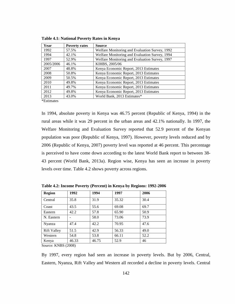
142
Table 4.1: National Poverty Rates in Kenya
Year Poverty rates Source
1992 57.5% Welfare Monitoring and Evaluation Survey, 1992
1994 42.1% Welfare Monitoring and Evaluation Survey, 1994
1997 52.9% Welfare Monitoring and Evaluation Survey, 1997
2005/2006 46.1% KIHBS, 2005/06
2007 48.8% Kenya Economic Report, 2013 Estimates
2008 50.8% Kenya Economic Report, 2013 Estimates
2009 50.5% Kenya Economic Report, 2013 Estimates
2010 49.8% Kenya Economic Report, 2013 Estimates
2011 49.7% Kenya Economic Report, 2013 Estimates
2012 49.8% Kenya Economic Report, 2013 Estimates
2013 43.0% World Bank, 2013 Estimates*
*Estimates
In 1994, absolute poverty in Kenya was 46.75 percent (Republic of Kenya, 1994) in the
rural areas while it was 29 percent in the urban areas and 42.1% nationally. In 1997, the
Welfare Monitoring and Evaluation Survey reported that 52.9 percent of the Kenyan
population was poor (Republic of Kenya, 1997). However, poverty levels reduced and by
2006 (Republic of Kenya, 2007) poverty level was reported at 46 percent. This percentage
is perceived to have come down according to the latest World Bank report to between 38-
43 percent (World Bank, 2013a). Region wise, Kenya has seen an increase in poverty
levels over time. Table 4.2 shows poverty across regions.
Table 4.2: Income Poverty (Percent) in Kenya by Regions: 1992-2006
Region 1992 1994 1997 2006
Central 35.8 31.9 35.32 30.4
Coast 43.5 55.6 69.08 69.7
Eastern 42.2 57.8 65.90 50.9
N. Eastern - 58.0 73.06 73.9
Nyanza 47.4 42.2 70.95 47.6
Rift Valley 51.5 42.9 56.33 49.0
Western 54.8 53.8 66.11 52.2
Kenya 46.33 46.75 52.9 46
Source: KNBS (2008)
By 1997, every region had seen an increase in poverty levels. But by 2006, Central,
Eastern, Nyanza, Rift Valley and Western all recorded a decline in poverty levels. Central
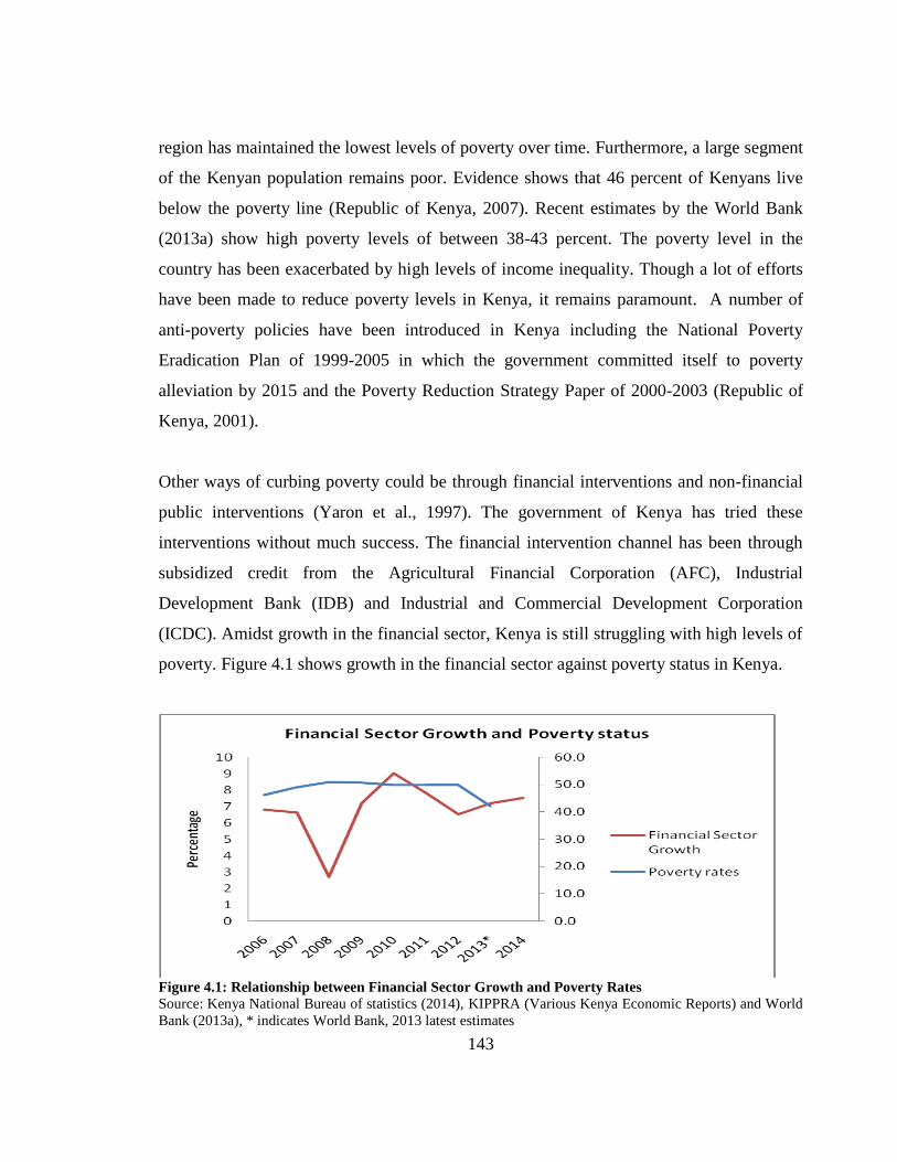
143
region has maintained the lowest levels of poverty over time. Furthermore, a large segment
of the Kenyan population remains poor. Evidence shows that 46 percent of Kenyans live
below the poverty line (Republic of Kenya, 2007). Recent estimates by the World Bank
(2013a) show high poverty levels of between 38-43 percent. The poverty level in the
country has been exacerbated by high levels of income inequality. Though a lot of efforts
have been made to reduce poverty levels in Kenya, it remains paramount. A number of
anti-poverty policies have been introduced in Kenya including the National Poverty
Eradication Plan of 1999-2005 in which the government committed itself to poverty
alleviation by 2015 and the Poverty Reduction Strategy Paper of 2000-2003 (Republic of
Kenya, 2001).
Other ways of curbing poverty could be through financial interventions and non-financial
public interventions (Yaron et al., 1997). The government of Kenya has tried these
interventions without much success. The financial intervention channel has been through
subsidized credit from the Agricultural Financial Corporation (AFC), Industrial
Development Bank (IDB) and Industrial and Commercial Development Corporation
(ICDC). Amidst growth in the financial sector, Kenya is still struggling with high levels of
poverty. Figure 4.1 shows growth in the financial sector against poverty status in Kenya.
Figure 4.1: Relationship between Financial Sector Growth and Poverty Rates
Source: Kenya National Bureau of statistics (2014), KIPPRA (Various Kenya Economic Reports) and World
Bank (2013a), * indicates World Bank, 2013 latest estimates

144
The financial sector has been growing with the exception of the year 2008 due to the post
election violence effects and 2012 due to the effects of the global financial crisis and fears
of the early 2013 general elections. The average growth rate of the financial sector has
been at about seven percent. However, poverty status has remained quite high at the ranges
of 46 percent. The 2013 poverty status is a World Bank estimate which indicates that
poverty has reduced slightly. However, this needs to be confirmed by the data that is
expected to be released by the KNBS through the Kenya Integrated Household and Budget
Survey in 2017. From the figure, it is not clear whether growth in the financial sector has
any impact on poverty status. It is this lack of clarity that motivates this study to look at
how financial development affects poverty in Kenya.
There have been efforts to grow the financial sector in the economy with an aim of
reducing poverty. Efforts were made to establish the Kenya Financial Sector Deepening
programme in the year 2005 to aid development of the financial markets with an aim of
stimulating wealth creation and reducing poverty. Even with all these efforts, many
Kenyans are still stuck in poverty and with little access to financial services (Kibua, 2007).
Financial access has increased with growth in mobile banking (FSD et al., 2016) but
poverty remains high. Evidence on the relationship between financial development and
poverty reduction particularly in Kenya is scant. Few studies such as Jalilian and
Kirkpatrick (2002) and Odhiambo (2010a and 2010b) investigated this relationship but the
unavailability of poverty data in various developing countries has made scholars to shy off
from this new debate. Thus, the link between financial development and poverty reduction
has been sidelined. In Kenya, few studies have investigated this relationship mainly
focusing on microfinance and poverty (Okibo and Makaga, 2014 and Kibua, 2007).
The country has experienced major financial developments and innovations in the last
decade. These developments and innovations may have had an effect on the poor in
society. But, it is not clear whether they have had any effect on poverty in Kenya or if there
actually is a failure of financial development to reduce poverty. Furthermore, the effect of
145
financial development on poverty is not yet known in terms of whether it is direct or
indirect through economic growth. Hence, these gaps lead to several questions: Which
channel of the effect of financial development on poverty dominates, the direct or the
indirect?; How does financial innovations, specifically M-Pesa, effect poverty?; What is
the nature of causality between financial development and poverty when the quality of the
financial sector is considered?
The main objective of this chapter was to investigate the relationship between financial
development and poverty in Kenya.
Specifically, the study sought to determine;
i) The direct and indirect effect of financial development on poverty
ii) The effect of financial innovation on poverty in Kenya
iii) The causality between financial development and poverty in Kenya
4.1.1 Significance of the Study
The relationship between financial development and poverty is important especially for a
country like Kenya. This study is important for policy makers in determining if financial
sector development spurs poverty reduction. It is also important for the policy makers to
establish how financial development reduces poverty, either directly or through economic
growth. This enables prioritization of where to place policy emphasis. Policy makers also
need to know how financial innovations impact on poverty reduction. The study also
contributes to the debate between financial development and poverty. Furthermore, it is
significant in demonstrating how quality and efficiency of financial development
determines the dynamics of the finance-poverty nexus.

146
4.2 Literature Review
4.2.1 Theoretical Literature
The theory of how the poor benefit from finance was brought about by Keynes (1937) who
discussed the motive of finance for money demand. The finance poverty theory can also be
traced from McKinnon (1973) on the conduit effect. The proposition was that a rise in
interest rate increases financial savings through financial intermediaries. Following from
Mckinnon, financial development affects poverty directly by allowing people to self-
finance their economic activities. Thus, the theory linking financial development and
poverty can be seen from two main fronts: the direct channel and the indirect channel. The
first one indicates a direct relationship between financial development and poverty
reduction while the second one is the trickledown theory whereby financial sector
development trickles down to the poor in the society through its stimulus on economic
growth. This follows the positive relationship existing in theory between financial
development and economic growth.
The direct channel has to do with financial market failures which include information
asymmetry especially in the credit market and high fixed costs of lending to small scale
borrowers. Financial deepening enhances access to formal finance by the poor. The direct
effect posits that financial development benefits the poor who do not have funds to self
finance their own projects. This implies that, financial development benefits the poor since
the poor are faced with credit constraints which are binding on them and thus they can‘t
access credit or finance for development due to lack of collateral (This was supported by
Aghio and Bolton, 1997). Thus, financial sector development reduces information
asymmetry and transaction costs thus allowing the poor to access finance (supported by
Fields, 2001). A poorly developed financial system creates more income inequality as it
keeps capital funds from reaching the very poor. Finally, financial development increases
productivity and increases the potential for the poor to achieve sustainable livelihoods
(World Bank, 2001). This is because improvement in the financial sector increases the

147
accessibility of the poor to financial services and thus enhancing their productive capacity
in terms of assets which then increases productivity and better sustainable lives. Thus, an
underdeveloped financial system leads to continued poverty, increased income inequality
and thus slows growth.
In regards to the trickledown theory or the indirect channel from financial development to
poverty through economic growth, there are a number of ways through which this happens.
First, growth promotes employment creation for the poor. Two, countries with higher
growth enables the governments to collect more revenues through taxes which can be
invested in health, education and social capital and which is beneficial to the poor. In
higher growth countries, the poor are also able to invest more in human capital and their
lives are greatly improved (Perroti, 1993). Thirdly, growth is seen to reduce wage
differentials between the skilled and unskilled population which is very beneficial to the
poor. However, this does not happen at the initial stages of development but rather at later
stages of development (Galor and Tsiddon, 1997). Finally, growth increases capital
accumulation in countries and thus they have more funds for investment purposes by the
poor which increases their incomes in the long term (Aghion and Bolton, 1997). This has
been criticized by studies which claim that capital accumulation arising from growth
generally benefits the haves and not the have-nots and thus can increase income inequality
in the long term (Haber, 2004).
4.2.2 Empirical Literature
Literature on financial development and poverty reduction is grounded on the direct
channel and the indirect channel through economic growth. The study thus reviewed the
empirical literature based on the channels of effect and direction of causality between
financial development and poverty reduction as well as measurement of financial
development and poverty.
148
a) Channels of the Effect of Financial Development on Poverty
A number of studies have found support for the indirect channel through economic growth
(Jalilian and Kirkpatrick, 2001, 2002 and 2005; Green et al., 2006; Odhiambo, 2009d and
Imram and Khali, 2012). They concluded that financial development leads to poverty
reduction by first affecting economic growth which then leads to poverty reduction. On the
other hand, studies like Pradhan (2010), Odhiambo (2010a) and Dhrifi (2013) supported
the theory that financial development does have a direct impact on poverty reduction.
There are also a number of studies which confirmed both theories in their findings like
Khan et, al. (2011), Dauda and Makinde (2014) and Kar et, al. (2015).
Several studies have also documented the indirect effect of financial development on
poverty reduction through growth. For example, financial development affects economic
growth through industrial growth (Imran and Khalil, 2012). Financial development is good
for industrial growth through access to credit while industrial growth leads to poverty
reduction in the long run. Additionally, Green et al. (2006) concluded that financial
development affects poverty through the development of Micro and Small Enterprises
(MSE). Financial sector development policies that encourage MSE growth do contribute to
poverty reduction in developing countries. However, this fact can only be realizable if the
MSE sector can be allowed access to credit that will foster its growth. This is because
access to credit has been singled out as the major impediment to the growth of the MSE
sector. Financial development has also been found to be pro-poor in developing countries
(Jeanneney and Kpodar, 2011) since it increases the incomes of the poor through higher
economic growth and increased access to finance and financial services for investment.
This view was further held by Jalilian and Kirkpatrick (2001 and 2002).
The direct channel intimated that financial development affects poverty directly by
allowing the poor to have access to credit (Dhrifi, 2013). Access to credit has been singled
out as the main hindrance to investment. Dhrifi (2013) supported this link in 89 developing
countries. The study found that the direct channel between financial development and
149
poverty reduction was robust and significant. The direct channel was through the access to
credit, insurance and savings channel. Financial development gives a chance to the poor to
accumulate savings for investment as well as avail micro insurance to cushion them from
adverse effects. Khan et al. (2011) also supported the importance of non-life insurance
access for the poor as an important way through which financial development affects
poverty. Green et al. (2006) also supported this direct channel by emphasizing on access to
credit.
The effect of inequality is seen to dampen the effect of financial development on poverty
through economic growth (Jalilian and Kirkpatrick, 2005 and Jeanneney and Kpodar,
2011). Inequality leads to benefits of financial development accruing to only a small
percentage of the population especially the high income population. Upto a certain level of
economic development, financial development leads to poverty reduction through the
growth channel after which due to inequality, financial development does not cause
poverty reduction (Jalilian and Kirkpatrick, 2005). Further, Dhrifi (2013) who found
support for the direct effect of financial development on poverty also found that inequality
hampers this effect. Dauda and Makinde (2014) found support for the indirect effect of
financial development on poverty in Nigeria. However, this effect is dampened by income
inequality in the long run leaving the direct effect to be dominant in the long run. Policy
makers should concentrate on tackling inequality.
Quality of institutions (Dhrifi, 2013) also matters for poverty. Financial institutions and
hence the quality of financial development which is low is found to dampen the effect of
financial development on the poor. Thus, including indicators which show the quality of
financial development is important so as to capture this dampening effect. The quality of
financial institutions can spur or deter physical and human capital investment as well as
determine transaction costs which will hinder or encourage the poor to use financial
services. Finally, financial instability affects the relationship between financial
development and poverty. Jeanneney and Kpodar (2011) supported the indirect effect of
150
financial development on poverty. However, financial instability which sometimes follows
financial development is found to be anti the poor as it stifles the positive effects of
financial development on poverty reduction.
b) Direction of Causality between Financial Development and Poverty
The second strand of literature shows the direction of causality between financial
development and poverty. A number of studies showed that financial development causes
poverty reduction (Jalilian and Kirkpatrick, 2002, Jalilian and Kirkpatrick, 2005; and
Jeanneney and Kpodar, 2011; Green et al., 2006; Odhiambo, 2009d; Pradhan, 2010;
Odhiambo 2010a, 2010b and Imran and Khalil, 2012) while a few showed that poverty
reduction can granger cause growth in the financial sector (Aye, 2013 and Uddin et al.,
2013b). Further, other studies showed that there is a bi-directional relationship between
financial development and poverty reduction (Sin-Yu and Odhiambo, 2011 and Uddin et
al., 2013b) while others showed that there is no causality between financial development
and poverty reduction (Fowowe & Abidoye, 2012 and Dandume, 2014).
Financial development causes poverty reduction directly through access to finance as some
studies posited (Odhiambo, 2010a; Odhiambo, 2010b and Pradhan, 2010) while others
found that poverty causes financial development through the growth route (Jalilian &
Kirkpatrick, 2002; Jeanneney & Kpodar, 2011 and Aye, 2013). On the causality from
poverty to financial development, Aye (2013) found that poverty granger causes financial
development but conditional on economic growth. Udddin et al. (2013) further controlled
for structural breaks in determining the causality between financial development and
poverty and found causality running from poverty to financial development. Some studies
have found that poverty is affected by other macro economic variables like trade openness
and inflation and hence there is no causality between financial development and poverty
reduction in SSA.
151
The direction of causality is found to be dependent on the financial development indicator
used (Odhiambo, 2010a; Odhiambo, 2010b and Sin-Yu and Odhiambo, 2011). Odhiambo
(2010a) for example conducted a study in Zambia using broad money supply, M2 and
domestic credit to private sector. On the one hand, when the study used broad money
supply, M2 as an indicator of financial development, it was found found that poverty
reduction led to the development of the financial sector. On the other hand, using domestic
credit to the private sector and bank assets as indicators of financial development, results
showed that financial sector development causes poverty reduction and concluded that it is
financial development that does cause poverty reduction. Sin – Yu and Odhiambo (2011)
found that in the long run, there is a bi-directional relationship between financial
development and poverty when domestic credit to private sector was used as a proxy for
financial development. There was also a weak bi-directional relationship in the short run
when M2 was used as a proxy for financial development but a unidirectional relationship
existed in the long run from poverty reduction to financial development.
c) Measurement of Financial Development and Poverty
Use of some financial development indicators and poverty measures has been criticized in
literature. Some of the financial development indicators mostly used in literature include
the monetization measure, broad money supply (Jeanneney and Kpodar, 2011; Odhiambo,
2009d; Odhiambo, 2010a; Odhiambo, 2010b; Pradhan, 2010; Sin-Yu and Odhiambo,
2011; Dhrifi, 2013; Dauda and Makinde, 2014 and Kar et al., 2015). This measure is a
monetization measure and does not show us the intermediation from surplus sectors to
deficit sectors. Further, this monetization measure is high in under developed and some
developing countries due to high currency and thus not a good measure of financial
development in these countries (Ang and Mckibbin, 2007; Dushku, 2010; Gehringer, 2013
and Dandume, 2014). Other studies used a financial depth measure, domestic credit
(Dhrifi, 2013). This measure shows the intermediation between those who have and those
who don‘t have. However, this measure includes credit to the public sector which may
crowd out private investment. The private sector is assumed to be more competitive and
152
thus able to allocate resources more efficiently. Thus, many other studies have used credit
to private sector as a measure of financial development (Jeanney and Kpodar, 2005;
Odhiambo, 2010a; Sin-Yu and Odhiambo, 2011; Uddin et al., 2012; Imran and Khalil,
2012; Fowowe and Abidoye, 2012; Dandume, 2014 and Kar et al., 2015).
Other financial development indicators used include Bank deposits to GDP (Jalilian and
Kirkpatrick, 2001; Jalilian and Kirkpatrick, 2002; Khan et al., 2011 and Dandume, 2014).
This measure was proposed to be a better measure of financial development since it
excludes currency which is high in developing countries. It also shows the ability of the
banking industry to mobilize savings and channel it to deficit productive sectors. Other
variables used include Net Foreign Assets (Jalilian and Kirkpatrick, 2001 and Jalilian and
Kirkpatrick, 2002), liquid assets to GDP (Jeanneney and Kpodar, 2011) which shows the
liquidity of the banking industry, domestic money bank assets (Jalilian and Kirkpatrick,
2002; Odhiambo, 2010a and Khan et al., 2011) which shows the total assets of the banking
industry and hence the stability of the industry, Central Bank assets (Khan et al., 2011),
real interest rate (Khan et al., 2011 and Dandume, 2014) as well as other non-bank
indicators like non-life insurance penetration, stock market turnover and bond market
capitalization (Khan et al., 2011).
Moreso, due to the various criticisms that come with the use of various financial
development indicators and due to the fact that these financial development indicators
cannot fully indicate the extent of financial development, some studies have chosen to use
a financial development index calculated through the use of Principal Component Analysis
using a number of these financial development indicators (Dhrifi, 2013 and Uddin et al.,
2013b). Use of different financial development indicators lead to different conclusions in
regards to the relationship between financial development and poverty.
These indicators show the financial depth, the liquidity of the banking sector, return on
savings as well as the contribution of non-bank sectors. These also do not show how

153
savings are converted into investments. They further do not show the quality of financial
development but just just the quantity. Financial development should not only show the
expansion of the financial sector in terms of quantity, it is also important to show the
quality and efficiency of this expansion. From the above discussion, the efficiency and
quality of financial development seem to have been ignored while it has been raised as
important in the relationship between financial development and poverty (Dhrifi, 2013).
Thus, it was important to include these aspects of financial development in the relationship
between financial development and poverty. Thus, the study adopts new financial
development indicators including non-performing loans and interest rate spread as well as
credit to private to show how savings are converted to investment.
On poverty measurement, per capita consumption has been used severally in literature to
measure poverty (Odhiambo, 2009d; Odhiambo, 2010a; Odhiambo, 2010b; Sin-Yu Ho and
Odhiambo, 2011; Uddin et al., 2012 and Kar et al., 2015. However, this measure is a
broader measure of welfare and not a direct measure of poverty. This may be necessitated
by the fact that poverty data in developing countries and especially in Africa is wanting
(Devarajan, 2013). Other literature has used Gini co-efficient as a measure of poverty
(Jalilian and Kirkpatrick, 2001 and Khan et al., 2011). This measure is however a measure
of income inequality and may not be a direct measure of poverty. Due to the limitations of
per capita consumption and Gini Coefficient as measures of poverty, studies have used
various other measures of poverty.
Head count ratio has been used (Jeanneney and Kpodar, 2011; Pradhan, 2010; Fowowe
and Abidoye, 2012; Dauda and Makinde, 2014 and Dandume, 2014) to show the
proportion of the population living below the poverty line – or on less than $ 1.25 per day
and average (per capita) incomes of the poor (Jalilian and Kirkpatrick, 2001; Jalilian and
Kirkpatrick, 2002 and Jeanneney and Kpodar, 2011). In Kenya, there are no studies done
using head count ration, poverty gap, poverty gap squared as measures of poverty to
determine the effect of financial development on poverty. This could be due to the scarcity
154
of this kind of data. Thus, this study broke the norm in Kenya to use head count ration to
analyse this relationship. The headcount ratio was calculated using the decomposition
method of income changes and gini-coefficient changes.
d) Data and Methodology
Other aspects of data and methodologies used lead to different results in regards to the
relationship between financial development and poverty. Several studies used time series
data to investigate this relationship. A number of methods have been used like granger
causality based on the (vector) error correction model (Odhiambo, 2009d; Odhiambo,
2010b and Kar et al., 2015), Granger causality models with cointegration and error
correction models (Pradhan, 2010 and Imran and Khalil, 2012), ARDL (Odhiambo, 2010a;
Sin–Yu and odhiambo, 2011; Uddin et al., 2012; Uddin et al., 2013b and Dandume, 2014),
VAR and Impulse Response Analysis (Dauda and Makinde, 2014). The use of these
methodologies leads to either the indirect effect or the direct effect as well as different
causality between financial development and poverty.
Other studies used panel and cross sectional analysis and found different results in regards
to the relationship between financial development and poverty. Jalilian and Kirkpatrick
(2001 and 2002) used OLS and panel 2SLS and found support for the indirect effect
through economic growth. Jeanneney and Kpodar (2011) also found support for the
indirect effect while using OLS and a dynamic panel GMM model. Jalilian and Kirkpatrick
(2005) further found support for the indirect effect using a reduced form model and an
explicit log-linear functional form equation. Aye (2013) also agreed with the indirect effect
of financial development on poverty through growth using GMM methodology. However,
Dhrifi (2013) found support for the direct effect using simultaneous equations estimated
through 3SLS while Khan et al. (2011) found support for both the direct and indirect
channels using OLS method of estimation.

155
In Kenya, studies on financial development and poverty done at a macro level are few
(Kibua, 2007 and Odhiambo, 2010b). Kibua (2007) in examining how access to financial
services reduces poverty found that in Kenya, the financial products including savings
offered by commercial banks are not in tune with the needs of the poor. Access to loans is
out of reach of the rural poor and they generally don‘t have access to affordable financial
services. The study however found that the poor borrow to invest in productive activities.
Odhiambo (2010b) included a third variable (savings) to check the direction of causality
between financial development and poverty. The study found support for causality from
financial development to poverty reduction. It used the monetization measure as an
indicator of financial development and per capita consumption as a measure of poverty.
Other studies done in Kenya on the relationship between financial development and
poverty were based on microfinance and include Hospes et al. (2002), Bakhtiari (2006),
Omunjala and Fondo (2014) and Okibo and Makanga (2014). Hospes et al. (2002) in
evaluating the impact of microfinance found that it is key in poverty reduction. Bakhtiari
(2006) indicated that microfinance has gained popularity as one of the leading ways of
reducing poverty. Besides, Kaburi et al. (2013) found that the rural poor do not have access
to formal financial services due to for example the fear of default by formal financial
institutions. Hence micro finance becomes very important in Kenya. Micro finance was
found to empower the rural poor. Other studies done at regional level included Kiiru
(2007), Okibo and Makanga (2014) and Omunjala and Fondo (2014). Kiiru (2007) found
that microfinance is helpful in reducing poverty in Makueni district as it increases the
households‘ income. Okibo and Makanga (2014) found that granting small loans to women
in the rural areas was used for productive investments including starting businesses,
expanding business as well as for educating their children. Thus micro finance is very
important in reducing poverty among the poor rural women in Kiambu district.
Tables 4.3 and 4.4 shows a summary of the literature in regards to channel of the effect of
financial development on poverty and direction of causality between the two.

156
Table 4.3: Summary of Findings of the Effect of Financial Development on Poverty
Studies Supporting the Indirect Channel of the Effect of Finance on Poverty through Economic Growth (Trickle down
hypothesis)
Author Methodology Findings
Imran and Khalil (2012) Time series; cointegration, ECM
A well functioning financial sector is key
for industrial growth and industrial
growth is important for poverty reduction
Odhiambo (2009d) Time series; Trivariate granger causality
based on the ECM
In both the short and the long run,
financial development leads to growth
while growth leads to poverty reduction. It is the real sector rather than the
financial sector that leads to poverty
reduction.
Jalilian and KirkPatrick (2005) Pooled panel data, reduced form model,
generic econometric model and explicit
log-linear functional form equation
Upto a certain level of development,
financial development leads to poverty
reduction. However, the effect of financial development on poverty
reduction is neutralized by inequality
Jalilian and Kirkpatrick (2002) OLS, 2SLS using panel data Indirect trickle-down effect of growth to
poverty reduction through financial
development using a sample of 26 developing countries.
Jalilian and Kirkpatrick (2001) OLS, Panel and 2 SLS Financial development directly leads to
poverty reduction and further the effect happens indirectly through economic
growth
Studies Supporting the Direct Channel between Finance and Poverty
Author Methodology Findings
Dhrifi (2013) 3SLS using a financial deepening index There is a direct effect from financial development to poverty reduction while
considering access to credit services, insurance and savings cannels
Odhiambo (2010a) Time series; cointegration-ARDL Financial sector development directly
leads to poverty reduction in Zambia
when domestic credit to private sector and domestic money bank assets are used as
indicators of financial development
Pradhan (2010) Cointegration and granger causality tests Financial development is important and has a direct impact on poverty reduction
Green et al. (2006) Previous literature Financial sector developments and
policies that affect Medium and Small
Enterprises lead to poverty reduction, Thus supporting the direct route channel
Studies Supporting both the Direct and Indirect Channels between Finance and Poverty
Author Methodology Findings
Kar et al. (2015) Cointegration and Granger causality based on VECM
Indirect channel through growth is confirmed and the direct channel though
evident, is weak in the short run.
Dauda and Makinde (2014) VAR and Impulse Response In the short run, the indirect channel
dominates while in the long run, the direct channel takes over
Khan et al. (2011) OLS Financial development leads to growth
while growth leads to poverty reduction. Further, the negative relationship between
financial development and poverty
reduction is verified
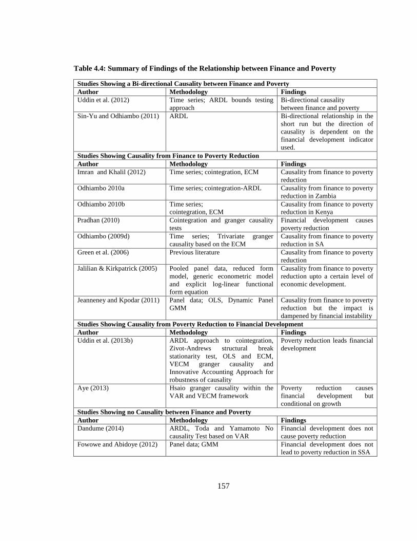
157
Table 4.4: Summary of Findings of the Relationship between Finance and Poverty
Studies Showing a Bi-directional Causality between Finance and Poverty
Author Methodology Findings
Uddin et al. (2012) Time series; ARDL bounds testing
approach
Bi-directional causality
between finance and poverty
Sin-Yu and Odhiambo (2011) ARDL Bi-directional relationship in the
short run but the direction of
causality is dependent on the
financial development indicator
used.
Studies Showing Causality from Finance to Poverty Reduction
Author Methodology Findings
Imran and Khalil (2012) Time series; cointegration, ECM
Causality from finance to poverty
reduction
Odhiambo 2010a Time series; cointegration-ARDL Causality from finance to poverty
reduction in Zambia
Odhiambo 2010b Time series;
cointegration, ECM
Causality from finance to poverty
reduction in Kenya
Pradhan (2010) Cointegration and granger causality
tests
Financial development causes
poverty reduction
Odhiambo (2009d) Time series; Trivariate granger
causality based on the ECM
Causality from finance to poverty
reduction in SA
Green et al. (2006) Previous literature Causality from finance to poverty
reduction
Jalilian & Kirkpatrick (2005) Pooled panel data, reduced form
model, generic econometric model
and explicit log-linear functional
form equation
Causality from finance to poverty
reduction upto a certain level of
economic development.
Jeanneney and Kpodar (2011) Panel data; OLS, Dynamic Panel
GMM
Causality from finance to poverty
reduction but the impact is
dampened by financial instability
Studies Showing Causality from Poverty Reduction to Financial Development
Author Methodology Findings
Uddin et al. (2013b) ARDL approach to cointegration,
Zivot-Andrews structural break
stationarity test, OLS and ECM,
VECM granger causality and
Innovative Accounting Approach for
robustness of causality
Poverty reduction leads financial
development
Aye (2013) Hsaio granger causality within the
VAR and VECM framework
Poverty reduction causes
financial development but
conditional on growth
Studies Showing no Causality between Finance and Poverty
Author Methodology Findings
Dandume (2014) ARDL, Toda and Yamamoto No
causality Test based on VAR
Financial development does not
cause poverty reduction
Fowowe and Abidoye (2012) Panel data; GMM
Financial development does not
lead to poverty reduction in SSA
158
4.2.3 Overview of Literature
Both theoretical and empirical literature show that financial development contributes to
poverty reduction. Some studies indicated that this happens indirectly through the
economic growth channel while others a direct channel through reduction in information
asymmetry and costs. Furthermore, different studies found support for causality from
financial development to poverty reduction, from poverty reduction and a bi-directional
relationship. There are no studies done in Kenya to determine whether its the direct or
indirect effects of financial development on poverty that prevail.
The cause of the differing results on both the channel of effect on poverty by financial
development and the direction of causality between the two could be the use of financial
development indicators which are inappropriate for a developing country, for example
Odhiambo, 2010b uses M2 as an indicator of financial development. This measure may be
inappropriate in developing countries since the largest component of M2 is currency and
does not appropriately show financial development (Dushku, 2010). Also, the studies done
in Kenya and many others on finance and poverty at a macro level have used per capita
consumption as a proxy for poverty. This measure has been criticized since it is a direct
measure of welfare and not poverty. Even with scanty availability of poverty time series
data, the study went ahead to calculate the poverty levels while making some realistic
assumptions as well as incorporating appropriate financial development indicators and
considering the quality aspects.
In addition, not considering the effect of structural breaks may lead to wrong conclusions
especially when it comes to the order of integration of variables. Moreover, the fact that
the effect of financial development on poverty reduction in developing countries cannot be
excluded from financial innovation and financial access, it was important to consider
financial innovations which tend to increase access to financial services which most of the
studies on financial development and poverty reduction do not include. Avais (2014)
indicated that financial innovation may be the only way that the poor can access financial

159
services. This is because innovative financial products are designed in a way that they can
target the poor. Thus, this study filled the gaps including, use of appropriate financial
development indicators, inclusion of financial innovation and robustness by using both per
capita consumption as well as head count ratio poverty measure and incorporating
structural breaks.
4.3 Methodology
4.3.1 Theoretical Framework
The theoretical link between finance and poverty can be traced back to the Mckinnon
conduit effect (Mckinnon 1973). The theory showed that financial development leads to
increase in domestic savings which is good for the poor as it then increases investment
undertaken by the poor. Thus, the theoretical link between financial development and
poverty reduction was positive. This was further exemplified by Jeanneney and Kpodar
(2011). This direct effect between financial development and poverty reduction can be
represented as:
),( ttt XFDfP …………………………………………………………………………..4.1
Where Pt is poverty, FDt is financial development and Xt are other control variables
affecting poverty.
Jeanneney and Kpodar (2011) in addition introduced the indirect effect of financial
development on poverty reduction through economic growth. More so, there is a lot of
literature that showed the importance of economic growth for poverty reduction (Nallari
and Griffith, 2011; Chhibber and Nayyar, 2007; Loayaza and Raddatz, 2006; Kraay, 2004;
Lopez, 2004 and Dollar and Kraay, 2002). These studies concluded that growth has a
positive and significant impact on poverty reduction. Thus, the indirect effect can be
represented by:

160
)( tt YfP ………………………………………………………………………………4.2
Where Pt is poverty and Yt is income growth.
However, literature shows that economic growth is a necessary but not sufficient condition
for poverty reduction (Moges, 2013; DFID, 2004 and Dollar and Kraay, 2002). Thus,
equation 4.2 becomes:
),( ttt XYfP ……………...…………………………………………………………..4.3
Where X represents other variables which affect and complement economic growth in
influencing poverty.
The indirect channel between financial development and poverty reduction can first be
considered by examining the effect of financial development on economic growth (this had
been examined in detail in chapter 3) which then has implications for poverty reduction.
Following Jalilian and Kirkpatrick (2001), this relationship is described by the following
system of equations:
1
'
1
'
11 WVy ..……….……………………………………………………4.4
2
''
2
''
22 WVp .….……………………………….……………………….4.5
Where y represents economic growth while p is a measure of poverty. V and W are vectors
of financial development indictors and other factors that affect poverty and economic
growth respectively. Jalilian and Kirkpatrick (2001) indicated that growth and poverty are
mostly affected by the same variables and the V and W vectors may include the same
variables but the effects would differ. Assuming the absence of simultaneity, then
equations 4.4 and 4.5 reduces to a reduced form equation as:
WVP ………………………………………………………………………………………………...4.6
161
4.3.2 Model Specification
In equation 4.3, financial development was our main variable of interest and it would be
included in the X vector. In equation 4.6, it would be represented in the V vector. A
number of financial development indicators have been used in the literature for example
broad money supply (M2), domestic credit (Kar et al., 2011 and Odhiambo, 2009) to show
the effect of financial development and poverty reduction. However, these measures have
been criticized in the literature since they are not appropriate financial development
indicators for underdeveloped countries (Dushku, 2010). In underdeveloped countries, the
currency composition in M2 is quite large and thus this measure does not show how the
financial intermediary channels funds from depositors to investors and thus the poor (Khan
and Senhadji, 2003).
This study utilized a new set of financial development indicators including non-performing
loans to show the efficiency of the financial sector, interest rate spread to show the
transactions cost as well as efficiency of the sector and how this may affect the poor‘s
access to credit as well as some of the indicators used in literature, bank credit to private
sector to show how funds are channeled from the ones who have to the ones who don‘t
have (poor). Market capitalization even if it had been included in the previous analysis is
left out in this chapter since there is a postulation that stock markets which are part of the
formal financial sector are not consistent with the needs of the poor but rather of the rich
(Bakhtiari, 2006). The study also added a measure of financial innovation (Krishnan, 2011)
since there has been a number of financial innovations in Kenya as these have led to an
increased access to financial services. The intuition is that financial innovations are seen to
be good for the poor.
Due to possible simultaneity, equation 4.6 was not estimated. Thus, following Dauda and
Makinde (2014) and Jalilian and Kirkpatrick (2001), an explicit linear equation derived
from equations 4.1 and 4.2 was estimated. Jalilian and Kirkpatrick (2001) asserted that
developing countries are more concerned than the developed ones with the Mckinnon

162
conduit effect or the direct channel rather than the indirect channel. This is because the
financial sector is more developed and vibrant in developed countries. Thus, the study
estimated an equation for the direct channel but include economic growth to capture the
indirect effect as follows:
tttttt FIZFDGDPPCP …..……….………...…………………..….4.7
Where Pt is poverty, GDPPCt is Gross Domestic Product per capita, FDt is the financial
development indicators which include non-performing loans (NPL), interest rate spread
(INT) and bank credit to private sector (CPS), FI is the financial innovation dummy and Zt
is other variables that affect poverty. Further, there is support in literature that inflation
negatively influences the poor (Easterly and Fischer, 2001 and Dollar and Kraay, 2002).
Other studies found that poverty is affected by trade openness which affects the savings
ratio of the population (Athukorala and Sen, 2004 and Christiaensen et al., 2003). Thus, the
study introduced these two variables as control variables to have:
ttttttt FITOINFFDGDPPCP …………….…………….……..4.8
Where INF is inflation and TO is trade openness and FDt is a vector of financial
development indicators including credit private sector, interest rate spread and non-
performing loans.
Equation 4.8 is expanded to include the financial development indicators and introducing
logarithms, the following equation is given:
ttttttttt FITOINFINTNPLCPSGDPPCP lnlnlnlnlnlnln
………………………………………….…………….……………………………..….4.9
Poverty was represented by head count ratio and per capita consumption as a measure of
welfare for robustness. ,,, gives us the direct effect while the coefficient gives the
163
indirect effect of financial development on poverty through growth. Taking the logarithms
of GDP per capita ensures that we have economic growth. It is assumed that financial
development is beneficial to the poor as it has a positive impact on economic growth.
4.3.3 Estimation and Testing
a) Descriptive Statistics
Descriptive statistics for all the variables were conducted to determine the statistical
properties of the model before running any estimation. This involved testing for the
skewness, kurtosis, normality of the variables and the spread of the data by determining the
mean and first movement from the mean.
b) Unit Root Tests
The study conducted unit root tests to eliminate the possibility of spurious regressions. It
used the usual Philip Perron (PP) test (Phillip and Perron, 1988) to determine presence of
unit root. Phillip Perron test results are preferred to ADF unit root test results because even
though the two tests give consistent results, the PP test has higher unit root detection
abilities (Baliamoune-Lutz, 2008). In addition, ignoring the presence of structural breaks
could lead to rejection of the null hypothesis (there is unit root) thus giving erroneous order
of integration of variables. Thus, the study went ahead to test for unit root using tests that
endogenously take into account the presence of structural breaks. It used the Zivot-
Andrews test (Zivot and Andrews, 1992) to test for unit root. This test considers only one
structural break which is determined endogenously. However, there are tests like
Clemente-Montanes-Reyes (1998) and Lumsdaine and Papell (1997) which takes into
account the presence of two structural breaks. However, these tests give similar results as
evident from chapter three. Thus, this study conducted only the Zivot – Andrews test. A
detailed description of the test was contained in chapter three.

164
c) Cointegration Analysis
It was important to test for cointegration since many macro-economic variables are likely
to have a stable long run relationship (Camillo, 2015). However, cointegration analysis is
conditional on variables having a unit root otherwise the normal OLS is used for analysis.
The intuition is that variables that are cointegrated will not move far away from each other
and thus their deviations are stationary in the long- run. This concept has been clearly
brought out by Murray (1994) in studying the drunk and her dog who will not lose sight of
each other. Variables which are non- stationary, a linear or many linear combinations of
these becomes stationary. This study used the Johansen cointegration test based on
Johansen (1988) and Johansen and Juselius (1990) which was based on the VAR model.
The Johansen test has two statistics, trace and max-eigen statistics which indicate whether
there is cointegration or not in the variables. The statistics are derived from observing the
rank of a long-run coefficient matrix which comprises a combination of the cointegrating
vectors as well as the amount of each cointegrating vector in each equation of the
VAR/VECM. The trace statistic is a joint test based on the null hypothesis that there is a
number of cointegrating equations equals to or less than the rank (r) against an alternative
hypothesis that the number of cointegrating equations is more than r. The max eigen
statistic is based on a null hypothesis that the number of cointegrating equations is r against
an alternative hypothesis that the number of cointegrating equations is equal to r+1.
d) VAR Model
Equation 4.9 was estimated using the VAR model introduced by Sims (1980). The VAR
model is advantageous because it does not require strong restrictions on parameters to be
imposed. It usually tests for joint behavior of variables which are treated as endogenous
from theory. The VAR methodology extends the Univariate Autoregressive Model by
including more than one varying variables. The choice of VAR was necessitated by the
fact other time series estimation methods like Autoregressive Lag Model requires variables
to be integrated of different orders, mainly 1(0) and 1(1). OLS would give spurious
165
regressions when variables are not stationary. A variation of the VAR model is the VECM
which allows the VAR model to determine relationships when the variables are
cointegrated or have a long run relation. The VECM allows for the errors in the short run
to be corrected in the long run by incorporating an error correction term as an explanatory
variable in the long run model.
The VECM is given by:
ttt
k
i
itit ECMFIZAZ
1
1
lnln
…….…….…………………………...4.10
Where Zt is a vector of variables which include poverty, financial development indicators
(credit to private sector, non-perfoming loans, interest rate spread), economic growth and
the control variables which include trade openness and inflation. Zt-i includes all the lagged
variables while FI indicate the financial innovation dummy. ECM is the error correction
term where ∏ is the coefficient of the error correction term and it gives the speed of
adjustment (of deviations) from the short run to the long run equilibrium.
The study then ran the granger causality test based on the VAR/VECM to determine the
causality between the variables. Further, tests for normality of residuals and
heteroscedasticity were performed.
4.3.4 Definition and Measurement of Variables Poverty is a multi-dimensional concept and in this study two measures of poverty were
used as the dependent variable. One of the measures which have been used in literature is
per capita consumption. However, this measure has been criticized in literature since it is a
general measure of welfare. Thus, the study went further to use head count ratio measure
of poverty for analysis. Head count ratio is defined as the number of the poor that lives
below the poverty line. It is calculated using the following formula:

166
t
i Z
YZ
NP
1
1
………………………….………………………………………...4.11
Where α is taken to be zero to give the head count ratio. Z is the poverty line, Y is income
and N is total population.
Since time series data on poverty in Kenya is scanty and thus getting annual headcount
ratio data was not possible, the study predicted head count poverty ratios based on the
methodology used by Ali and Thorbecke (2000) and Mwabu et al. (2003). The study used
the poverty changes decomposition method which follows from the notion that what cause
changes in poverty over time is mostly changes in income growth and income distribution
(Mwabu et al., 2003 and Ali and Thorbecke, 2000) where the effect is negative for positive
changes in income growth and positive for positive changes in inequality. This relationship
is specified as:
iiii GingP .............................................................................................4.12
Where P is poverty in year i and Gin is the Gini-coefficient (measure of income
distribution). and gives the effects of Economic growth and income distribution on
poverty for a certain year and is a constant. Thus the changes in poverty can be given by
the following equation which shows changes in both income growth and income
distribution. is a constant while is the error term with an expectation of zero.
GinGDPP …………………………………………………………………5.13
Where Δ means change. The co-efficients α, β and δ are hard to get in some countries since
annual data is unavailable mostly in these underdeveloped and some developing countries
like Kenya. Thus, this study followed Mwabu et al. (2003) by obtaining these coefficients
from Ali and Thorbecke (2000) who estimated poverty regressions to determine the state
and path of poverty in Sub Saharan African countries, Kenya included. This cross-country
study results showed that values of α, β and δ were more or less the same across the
167
various countries. Further, Mwabu et al. (2003) and Odhiambo et al. (2005) made the
assumptions that the coefficients can be used for different countries and for post Ali and
Thorbecke study‘s period. The idea is that poverty elasticities to income growth and
inequality were found to be almost the same across different countries and across regions
in one country. Thus, the study followed the same assumptions and continued to predict
the poverty rates using the coefficients α, β and δ which are reported in Tables A.11, A.12
and A.13 (Appendix). Changes in poverty were calculated using equation 4.12. However,
changes in inequality are hard to get in Kenya since there is no quarterly Gini coefficients
data and even the yearly ones are intermittent. The study thus ignored the changes the Gini
coefficient and used only changes in income growth to predict headcount ratio. The
predicted head count ratio is given in Table A.20 (Appendix).
Per capita consumption is defined as the value of all goods and services purchased by
households divided by population. It is used as a measure of poverty and justified in
literature since World Bank defines poverty as ―the inability to attain a minimal standard of
living‖ which is defined in consumption terms. Further, it is taken to be more reliable and
correct than income (Woolard and Leibbrandt, 1999 and Odhiambo, 2009). Per capita
consumption is a measure of welfare and not a direct measure of poverty. It is used as a
welfare measure having implications on poverty. Spicker (2002) implied that welfare and
the welfare state usually help in reducing poverty. Welfare is designed to stop people from
falling into poverty. Further, Fording and Berry (2007) found that increased welfare is
important for poverty reduction although the effect of welfare programs on poverty has
reduced over time. Thus, the study used per capita consumption which is a measure of
welfare with an implied poverty effect.
However, the per capita consumption data is on an annual basis while quarterly data was
required. The study thus used the quadratic match sum formula in Eviews statistical
programme. This formula is advantageous when the data points being interpolated to a
higher frequency are relatively few and fairly even or consistent. Quadratic match sum
168
usually has a quadratic polynomial for each of the original data series. Picking three
adjacent data points, one before and one after (and for end points taking data points from
the side where data is available), a quadratic polynomial is fitted to produce the quarterly
data points such that either the sum or the average of these quarterly points equals the low
frequency data observed.
GDP per capita is defined as the Gross Domestic Product divided by the total population. It
is a measure of the total output or total product of a country. Its measurement is the same
as the per capita consumption. Financial development is proxied by bank credit to private
sector to GDP, non- performing loans to total loans and interest rate spread. These are as
defined in chapter two and Table 3.5. Further, financial innovation is defined as the
creation of a new product or institution into the financial system. In this case, financial
innovation is represented by M-Pesa volumes since its onset in 2007 but due to
unavailability of enough data observations, the study introduced a financial innovation or
M-Pesa dummy to represent existence (takes the value of 1) and absence (takes the value
of 0) of M-Pesa and hence presence and absence of M-Pesa volumes. The presence of M-
Pesa as a financial innovation is important since it has benefitted people through the
channels of increased transactions, transfers, savings and credit. These channels have not
only increased access to credit but also dealt with the problems of non-convexities in the
financial sector through its flexibility in terms of lending amounts and collateral.
It is theoretically expected apriori that GDP per capita, bank credit to private sector,
financial innovation and trade openness would be beneficial to the poor by enabling them
to self-finance themselves (Mckinnon, 1973), offering them proper access to good and
services and improve their wellbeing. Hence, the relationship between these variables and
head count ratio was expected to be negative but positive with per capita consumption.
Interest rate spread, non-performing loans and inflation were expected apriori to be
deleterious to the poor since interest rate spread show high transaction costs, non-
performing loans, the inefficiency of the financial sector and inflation erodes the
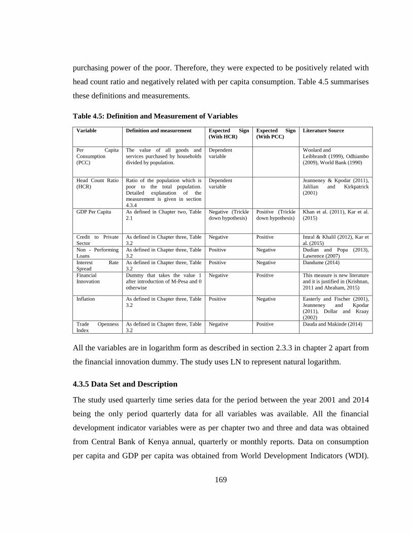
169
purchasing power of the poor. Therefore, they were expected to be positively related with
head count ratio and negatively related with per capita consumption. Table 4.5 summarises
these definitions and measurements.
Table 4.5: Definition and Measurement of Variables
Variable Definition and measurement Expected Sign
(With HCR)
Expected Sign
(With PCC)
Literature Source
Per Capita
Consumption
(PCC)
The value of all goods and
services purchased by households
divided by population.
Dependent
variable
Woolard and
Leibbrandt (1999), Odhiambo
(2009), World Bank (1990)
Head Count Ratio
(HCR)
Ratio of the population which is
poor to the total population.
Detailed explanation of the measurement is given in section
4.3.4
Dependent
variable
Jeanneney & Kpodar (2011),
Jalilian and Kirkpatrick
(2001)
GDP Per Capita As defined in Chapter two, Table
2.1
Negative (Trickle
down hypothesis)
Positive (Trickle
down hypothesis)
Khan et al. (2011), Kar et al.
(2015)
Credit to Private
Sector
As defined in Chapter three, Table
3.2
Negative Positive Imral & Khalil (2012), Kar et
al. (2015)
Non - Performing Loans
As defined in Chapter three, Table 3.2
Positive Negative Dudian and Popa (2013), Lawrence (2007)
Interest Rate
Spread
As defined in Chapter three, Table
3.2
Positive Negative Dandume (2014)
Financial Innovation
Dummy that takes the value 1 after introduction of M-Pesa and 0
otherwise
Negative Positive This measure is new literature and it is justified in (Krishnan,
2011 and Abraham, 2015)
Inflation As defined in Chapter three, Table
3.2
Positive Negative Easterly and Fischer (2001),
Jeanneney and Kpodar (2011), Dollar and Kraay
(2002)
Trade Openness
Index
As defined in Chapter three, Table
3.2
Negative Positive Dauda and Makinde (2014)
All the variables are in logarithm form as described in section 2.3.3 in chapter 2 apart from
the financial innovation dummy. The study uses LN to represent natural logarithm.
4.3.5 Data Set and Description
The study used quarterly time series data for the period between the year 2001 and 2014
being the only period quarterly data for all variables was available. All the financial
development indicator variables were as per chapter two and three and data was obtained
from Central Bank of Kenya annual, quarterly or monthly reports. Data on consumption
per capita and GDP per capita was obtained from World Development Indicators (WDI).
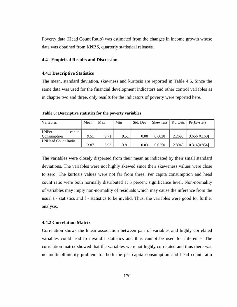
170
Poverty data (Head Count Ratio) was estimated from the changes in income growth whose
data was obtained from KNBS, quarterly statistical releases.
4.4 Empirical Results and Discussion
4.4.1 Descriptive Statistics
The mean, standard deviation, skewness and kurtosis are reported in Table 4.6. Since the
same data was used for the financial development indicators and other control variables as
in chapter two and three, only results for the indicators of poverty were reported here.
Table 6: Descriptive statistics for the poverty variables
Variables Mean Max Min Std. Dev. Skewness Kurtosis Pr(JB-stat)
LNPer capita
Consumption 9.51 9.71 9.51 0.08 0.6028 2.2698 3.656[0.160]
LNHead Count Ratio 3.87 3.93 3.81 0.03 0.0250 2.8940 0.314[0.854]
The variables were closely dispersed from their mean as indicated by their small standard
deviations. The variables were not highly skewed since their skeweness values were close
to zero. The kurtosis values were not far from three. Per capita consumption and head
count ratio were both normally distributed at 5 percent significance level. Non-normality
of variables may imply non-normality of residuals which may cause the inference from the
usual t - statistics and f - statistics to be invalid. Thus, the variables were good for further
analysis.
4.4.2 Correlation Matrix
Correlation shows the linear association between pair of variables and highly correlated
variables could lead to invalid t statistics and thus cannot be used for inference. The
correlation matrix showed that the variables were not highly correlated and thus there was
no multicollinierity problem for both the per capita consumption and head count ratio
171
models. However, the positive and negative relationships between the variables were
evident as indicated in Table A.12 and A.13 in Appendix.
4.4.3 Unit Root Tests
a) Optimal Lag Length
It was important to determine the optimal lag length for all the variables in order to
continue with further tests on unit root. As for the financial development indicators and the
control variables, the optimal lag length had been determined in chapter three. GDP per
capita, Credit to Private Sector, non-performing loans, interest rate spread, inflation and
trade openness had 2, 3, 1, 3, 1, 4 and 3 optimal lag length respectively (Refer to Table A.1
in appendix). As for per capita consumption, all the optimal lag length selection criterias
showed the same lag length of two while for the headcount ratio was found to have an
optimal lag of one.
b) Graphical Representation of the Variables
Before running the unit root tests, a graphical analysis of the variables was important to
show whether the variables have a deterministic trend or not. The graphs showed that both
per capita consumption and GDP per capita have a trend. However, it was not possible to
tell whether headcount ratio has a trend or not. These graphs were indicated in Appendix.
c) Unit Root Test Results
The study estimated the Phillip Perron unit root tests and the Zivot – Andrews test which
takes into account the presence of structural breaks and the results were given in Tables 5.7
for Phillip Perron test. All the financial development indicators and control variables had
been tested for unit root and the results showed that they were all integrated of order 1
(Refer to Tables 2.2 and 3.3 in chapter two and three respectively). Therefore, we show
results for per capita consumption and headcount ratio.

172
Table 4.7: Phillip Perron Unit Root Test Results
At levels 1st difference Order of
integratio
n
Constant Trend &
Intercept
Constant Trend &
Intercept
Variables t-stat 5%
Critical
value
t-stat 5%
Critical
value
t-stat 5%
Critical
value
t-stat 5%
Critica
l value
LNPer
Capita
Consumption
0.895 -2.916 -1.866 -3.495 -3.037 -2.916 -3.529 -3.495 1(1)
LNHead
Count Ratio
-1.831 -2.915 -2.126 -3.493 -7.204 -2.916 -7.139 -3.495 1(1)
Phillip Perron test for unit root showed that per capita consumption and Head Count Ratio
had a unit root but were stationary at first difference at 5 percent significance level. Test
results for Zivot Andrews did not show any different results from the Phillip Perron results
in terms of presence of unit root. The variables were integrated of order one. The test also
endogenously determined the years of structural break for each variable with per capita
consumption having a structural break at quarter two of 2007 and head count ratio at
quarter three of 2005. We also show results for Zivot-Andrews unit root test for the two
variables. These are shown in Table 4.8.
Table 4.8: Zivot-Andrews Unit Root Test Results for Poverty Measures
Trend & Intercept
Variables Year of
structural
break
Level First Difference Order of
integratio
n t-stat 5%
Critical
value
t-stat 5% Critical
value
LNPer Capita
Consumption
2007q2 -3.121 -5.08 -6.899 -5.08 1(1)
LNHead Count Ratio 2005q3 -3.578 -5.08 -8.097 -5.08 1(1)
The results showed that the per capita consumption and head count ratio were not
stationary at levels but stationary at first difference. Thus, they reinforced the results of the
Phillip-Perron unit root test.
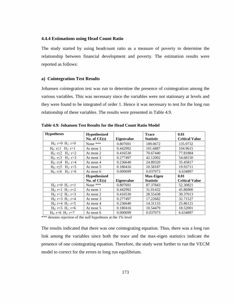
173
4.4.4 Estimations using Head Count Ratio
The study started by using headcount ratio as a measure of poverty to determine the
relationship between financial development and poverty. The estimation results were
reported as follows:
a) Cointegration Test Results
Johansen cointegration test was run to determine the presence of cointegration among the
various variables. This was necessary since the variables were not stationary at levels and
they were found to be integrated of order 1. Hence it was necessary to test for the long run
relationship of these variables. The results were presented in Table 4.9.
Table 4.9: Johansen Test Results for the Head Count Ratio Model
Hypotheses Hypothesized
No. of CE(s) Eigenvalue
Trace
Statistic
0.01
Critical Value
H0: r=0 H1: r>0 None *** 0.807691 189.0672 135.9732
H0: r≤1 H1: r>1 At most 1 0.442992 101.6887 104.9615
H0: r≤2 H1: r>2 At most 2 0.416530 70.67440 77.81884
H0: r≤3 H1: r>3 At most 3 0.277497 42.12002 54.68150
H0: r≤4 H1: r>4 At most 4 0.236640 24.89320 35.45817
H0: r≤5 H1: r>5 At most 5 0.180416 10.58187 19.93711
H0: r≤6 H1: r>6 At most 6 0.000699 0.037073 6.634897
Hypothesized
No. of CE(s) Eigenvalue
Max-Eigen
Statistic
0.01
Critical Value
H0: r=0 H1: r=1 None *** 0.807691 87.37843 52.30821
H0: r=1 H1: r=2 At most 1 0.442992 31.01432 45.86900
H0: r=2 H1: r=3 At most 2 0.416530 28.55438 39.37013
H0: r=3 H1: r=4 At most 3 0.277497 17.22682 32.71527
H0: r=4 H1: r=5 At most 4 0.236640 14.31133 25.86121
H0: r=5 H1: r=6 At most 5 0.180416 10.54479 18.52001
H0: r=6 H1: r=7 At most 6 0.000699 0.037073 6.634897
*** denotes rejection of the null hypothesis at the 1% level
The results indicated that there was one cointegrating equation. Thus, there was a long run
link among the variables since both the trace and the max-eigen statistics indicate the
presence of one cointegrating equation. Therefore, the study went further to run the VECM
model to correct for the errors to long run equilibrium.
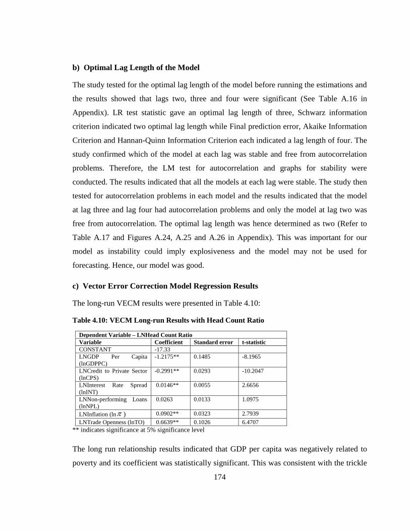
174
b) Optimal Lag Length of the Model
The study tested for the optimal lag length of the model before running the estimations and
the results showed that lags two, three and four were significant (See Table A.16 in
Appendix). LR test statistic gave an optimal lag length of three, Schwarz information
criterion indicated two optimal lag length while Final prediction error, Akaike Information
Criterion and Hannan-Quinn Information Criterion each indicated a lag length of four. The
study confirmed which of the model at each lag was stable and free from autocorrelation
problems. Therefore, the LM test for autocorrelation and graphs for stability were
conducted. The results indicated that all the models at each lag were stable. The study then
tested for autocorrelation problems in each model and the results indicated that the model
at lag three and lag four had autocorrelation problems and only the model at lag two was
free from autocorrelation. The optimal lag length was hence determined as two (Refer to
Table A.17 and Figures A.24, A.25 and A.26 in Appendix). This was important for our
model as instability could imply explosiveness and the model may not be used for
forecasting. Hence, our model was good.
c) Vector Error Correction Model Regression Results
The long-run VECM results were presented in Table 4.10:
Table 4.10: VECM Long-run Results with Head Count Ratio
Dependent Variable – LNHead Count Ratio
Variable Coefficient Standard error t-statistic
CONSTANT -17.33
LNGDP Per Capita
(lnGDPPC)
-1.2175** 0.1485 -8.1965
LNCredit to Private Sector
(lnCPS)
-0.2991** 0.0293 -10.2047
LNInterest Rate Spread
(lnINT)
0.0146** 0.0055 2.6656
LNNon-performing Loans
(lnNPL)
0.0263 0.0133 1.0975
LNInflation (ln ) 0.0902** 0.0323 2.7939
LNTrade Openness (lnTO) 0.6639** 0.1026 6.4707
** indicates significance at 5% significance level
The long run relationship results indicated that GDP per capita was negatively related to
poverty and its coefficient was statistically significant. This was consistent with the trickle

175
down hypothesis of financial development on poverty through growth. A one percent
increase in GDP per capita reduces poverty by 1.22 percent which is a very high elasticity.
This indicated that growth is good for the poor and is in line with various studies in
literature (Imral and Khalil, 2012; Jalilian and KirkPatrick, 2005; Loayaza and Raddatz,
2006 and Dollar and Kraay, 2002) that showed the importance of growth for poverty. On
the financial development indicators, the coefficient of non-performing loans was positive
and not statistically significant but the one for credit to private sector was significant and
negatively related to poverty while the coefficient of interest rate spread was significant
and positively related to poverty. Credit to private sector is thus good for the poor as it
reduces poverty. This was expected from theory and literature since credit can be used to
smooth consumption and for investment purposes (Dembiermont, 2013) and thus
increasing incomes of the poor. This implies that they can invest more as they continue
borrowing and eventually leave the poor well off than without access to credit.
Interest rate spread was positively related to poverty and the coefficient was statistically
significant. An increase in interest rate spread by one percent increases poverty by 0.01
percent. According to theory, high interest rate spread indicates high transaction costs
hence an inefficient financial sector (Holden and Prokopenko, 2001). These results were
consistent with Khan et al. (2011) and Dandume (2014) that a high interest rate spread is
bad for the poor. The coefficients of the control variables were significant in affecting
poverty. Trade openness was positively related with head count ratio and the coefficient
was significant. Trade is theoretically supposed to reduce poverty due to increased
productivity and growth as argued by Adam Smith. As trade openness increases by one
percent, head count ratio increases by 0.66 percent. This implied that trade is bad for the
poor. Singh and Le Goff (2013) indicated that trade maybe bad for the poor if it is not
accompanied by other policies in other sectors especially the financial sector and if it is not
complemented by other investments like in human capacity as well as governance
building. Inflation is also bad for the poor as indicated by Easterly and Fischer (2001). The
coefficient of inflation was statistically significant and positive. A one percent increase in

176
inflation leads to 0.09 percent increase in poverty. Inflation reduces the purchasing power
for the poor thus making them worse off.
Thus, the results supported the trickle down hypothesis that financial development affects
poverty through economic growth. Further, the effect of financial development on poverty
was indicated by two of the financial development indicators (credit to private sector and
interest rate spread) implying that financial development is important for poverty reduction
both directly and also through economic growth.
d) Short -run Relationship Results
It was necessary to show the short-run relationships between financial development and
poverty after showing the long-run relationships so as to give the error correction model
results. The short-run analysis uses differenced variables which is represented by D. These
were shown in Table 4.11
Table 4.11: Short-run Relationship on VECM with Head Count Ratio
Dependent Variable – DLNHead Count Ratio
Variable Coefficient Standard
error
t-statistic
DLNHead Count Ratio (-1) 0.0050 0.2355 0.2124
DLNHead Count Ratio (-2) 0.2101** 0.0088 2.3825
DLNGDP Per Capita (-1) -1.1108 0.8126 -1.3671
DLNGDP Per Capita (-2) -1.3071** 0.5124 -2.5511
DLNCredit to Private Sector (-1) -1.6439** 0.6568 -2.5028
DLNCredit to Private Sector (-2) -0.0406 0.0968 -0.4196
DLNInterest Rate Spread (-1) 0.4209** 0.1254 3.3580
DLNnterest Rate Spread (-2) 0.0114 0.0108 1.0453
DLNNon-performing Loans (-1) -0.0598 0.0422 -0.1419
DLNNon-performing Loans (-2) 0.0956** 0.0465 2.0553
Mobile Payments Dummy
(MPAYDU)
-0.1873** 0.0814 -2.2995
Error Correction Term (ECMt-1) -0.0741** 0.0254 -2.9103
** indicates significance at 5% significance level
On the short run relationship, the coefficient of head count ratio was significant at lag two
implying that poverty affects itself negatively with a lag. Poverty today causes more
poverty tomorrow. This is according to the poverty trap theory (Sachs, 2005) which
177
proposes that poverty begets poverty or the fact that poverty today leads to the persistence
of poverty. This is the reason for inclusion of the lagged head count ratio. A one percent
increase in poverty today leads to a 0.21 percent increase in poverty two quarters after.
One reason why this increase in poverty would be less would be the accompanying effects
of the indirect effect where growth significantly lowers poverty. GDP per capita also
affects poverty negatively in lag two. The coefficient was also statistically significant. A
one percent increase in GDP per capita reduces headcount ratio by 1.30 percent.
The trickledown effect of economic growth on poverty happens with two lags. On
financial development indicators, all the coefficients of the variables were significant. The
effect of credit to private sector was negative meaning that it is good for the poor in the
short run. An increase in credit to private sector by one percent reduces poverty by 1.64
percent. This was consistent with existing literature (Kar et al., 2015 and Imral and Khalil,
2012). Access to credit leads to increased investment activities which is good for the poor.
Interest rate spread was positively related to poverty in the short run implying that lower
transaction costs promote the poor to access credit. The control variables were not
statistically significant in the short run.
Financial innovation (represented by MPAYDU dummy) was negatively related to poverty
and the coefficient was statistically significant. Use of M-Pesa reduces poverty by 17.30
percent. This finding was as expected that financial innovations are good for the poor. In
our study, it implied that the introduction of M-Pesa has been beneficial to the poor. This
beneficial impact can be seen from several fronts both from the transfers channel and the
credit channel. Transfers through M-Pesa increase the incomes of the poor for both
consumption and investments purposes. This result could also imply that once the poor
receive transfers, they use it for food consumption hence reducing food poverty. On the
credit channel, M-Pesa through M-Shwari has increased the poor‘s access to credit. M-

178
Shwari allows flexibility, requires no collateral and deals with the non convexities17
of the
financial sector which is associated with market failures. This is because monthly income
as a prerequisite to borrowing is not required. Further, M-Shwari allows people to borrow
low amounts of between Kenya shilling 50 to 100,000. The formal financial sector does
not allow access to credit of such small amounts; hence M-Shwari has closed this gap and
thus dealt with the non-convexities of the formal financial sector.
In the head count ratio model, the error correction coefficient was negative and significant.
It showed that, in each quarter 7.4 percent of the deviations were corrected. This implied
that for the system to equilibrate in the long run, it would take about 14 quarters or about
three and a half years.
e) VEC Granger Causality Results
The results of the granger causality using Wald test to show the direction of causality
between financial development and poverty were indicated in Table 4.12. The variables
were in first difference and natural logarithm.
17
Indicate the situation where the formal financial sector is unable to take care of the needs of the poor. It
only affords credit for the rich and the middle income leaving out the poor.
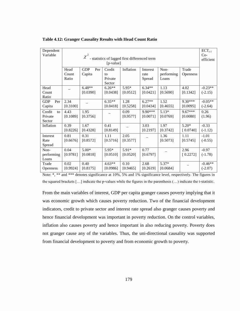
179
Table 4.12: Granger Causality Results with Head Count Ratio
Dependent
Variable
2
- statistics of lagged first differenced term
[p-value]
ECTt-1
Co-
efficient
Head
Count
Ratio
GDP Per
Capita
Credit
to
Private
Sector
Inflation Interest
rate
Spread
Non-
performing
Loans
Trade
Openness
Head
Count
Ratio
_ 6.48**
[0.0390]
6.26**
[0.0438]
5.95*
[0.0512]
6.34**
[0.0421]
1.13
[0.5690]
4.02
[0.1342]
-0.23**
(-2.15)
GDP Per
Capita
2.34
[0.3100]
_ 6.35**
[0.0418]
1.28
[0.5258]
6.27**
[0.0434]
1.52
[0.4655]
9.30***
[0.0095]
-0.05**
(-2.64)
Credit to
Private
Sector
4.43
[0.1089]
1.95
[0.3756]
_ 0.09
[0.9577]
9.90***
[0.0071]
5.13*
[0.0769]
9.67***
[0.0080]
0.26
(1.96)
Inflation 0.39
[0.8226]
1.67
[0.4328]
0.41
[0.8149]
_ 3.03
[0.2197]
1.97
[0.3742]
5.20*
[ 0.0740]
-0.33
(-1.12)
Interest
Rate
Spread
0.81
[0.6676]
0.31
[0.8572]
1.11
[0.5716]
2.05
[0.3577]
_ 1.36
[0.5073]
1.11
[0.5745]
-1.01
(-0.55)
Non-
performing
Loans
0.04
[0.9781]
5.00*
[0.0818]
5.95*
[0.0510]
5.91*
[0.0520]
0.77
[0.6797]
_ 2.96
[ 0.2272]
-0.97
(-1.78)
Trade
Openness
0.02
[0.9924]
0.40
[0.8175]
4.63**
[0.0986]
0.10
[0.9465]
2.68
[0.2619]
5.37*
[0.0684]
_ -0.46**
(-2.07)
Note: *, ** and *** denotes significance at 10%, 5% and 1% significance level, respectively. The figures in
the squared brackets […] indicate the p-values while the figures in the parenthesis (…) indicate the t-statistic.
From the main variables of interest, GDP per capita granger causes poverty implying that it
was economic growth which causes poverty reduction. Two of the financial development
indicators, credit to private sector and interest rate spread also granger causes poverty and
hence financial development was important in poverty reduction. On the control variables,
inflation also causes poverty and hence important in also reducing poverty. Poverty does
not granger cause any of the variables. Thus, the uni-directional causality was supported
from financial development to poverty and from economic growth to poverty.
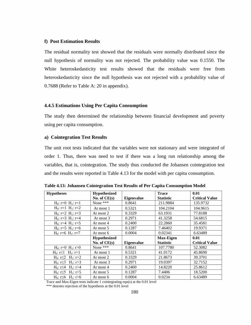
180
f) Post Estimation Results
The residual normality test showed that the residuals were normally distributed since the
null hypothesis of normality was not rejected. The probability value was 0.1550. The
White heteroskedasticity test results showed that the residuals were free from
heteroskedasticity since the null hypothesis was not rejected with a probability value of
0.7688 (Refer to Table A: 20 in appendix).
4.4.5 Estimations Using Per Capita Consumption
The study then determined the relationship between financial development and poverty
using per capita consumption.
a) Cointegration Test Results
The unit root tests indicated that the variables were not stationary and were integrated of
order 1. Thus, there was need to test if there was a long run relationship among the
variables, that is, cointegration. The study thus conducted the Johansen cointegration test
and the results were reported in Table 4.13 for the model with per capita consumption.
Table 4.13: Johansen Cointegration Test Results of Per Capita Consumption Model
Hypotheses Hypothesized
No. of CE(s) Eigenvalue
Trace
Statistic
0.01
Critical Value
H0: r=0 H1: r=1 None *** 0.8641 211.9884 135.9732
H0: r=1 H1: r=2 At most 1 0.5321 104.2104 104.9615
H0: r=2 H1: r=3 At most 2 0.3329 63.1931 77.8188
H0: r=3 H1: r=4 At most 3 0.2971 41.3258 54.6815
H0: r=4 H1: r=5 At most 4 0.2400 22.2860 35.4581
H0: r=5 H1: r=6 At most 5 0.1287 7.46402 19.9371
H0: r=6 H1: r=7 At most 6 0.0004 0.02341 6.63489
Hypothesized
No. of CE(s) Eigenvalue
Max-Eigen
Statistic
0.01
Critical Value
H0: r=0 H1: r>0 None *** 0.8641 107.7780 52.3082
H0: r≤1 H1: r>1 At most 1 0.5321 41.0172 45.8690
H0: r≤2 H1: r>2 At most 2 0.3329 21.8673 39.3701
H0: r≤3 H1: r>3 At most 3 0.2971 19.0397 32.7152
H0: r≤4 H1: r>4 At most 4 0.2400 14.8220 25.8612
H0: r≤5 H1: r>5 At most 5 0.1287 7.4406 18.5200
H0: r≤6 H1: r>6 At most 6 0.0004 0.0234 6.63489 Trace and Max-Eigen tests indicate 1 cointegrating eqn(s) at the 0.01 level
*** denotes rejection of the hypothesis at the 0.01 level

181
Both the trace and Max-Eigen statistics indicated that there was one cointegrating vector.
Thus, there was a long-run relationship or link among the variables as cointegration was
found. Thus, the VAR model could not be used. The study therefore estimated the VECM
that corrects for the error between the short run and the long run.
b) Optimal Lag Length
Before running VECM model, the study tested for the optimal lag length of the model and
the results were given in Table A.14 in Appendix. LR test statistic, Final prediction error,
Akaike information criterion and Hannan-Quinn information criterion for determining the
lag length all indicated an optimal lag length of four while the Schwarz information
criterion indicated a lag length of two. The study therefore went further to determine which
of these lags gave a stable model and free of autocorrelation. The results for stability and
autocorrelation were given in Table A.15 and Figure A.23 in Appendix. The stability tests
showed that the model at both lags was stable but the model at lag four suffered from
autocorrelation problems. Therefore the optimal lag length was determined as two.
c) Vector Error Correction Model Regression Results
Table 4.14: VECM Results – Long-run Relationship with Per Capita Consumption
Dependent Variable – LNPer Capita Consumption
Variable Coefficient Standard error t-statistic
CONSTANT 1.34**
LNGDP Per Capita (lnGDPPC) -1.2392** 0.0752 -16.4841
LNCredit to Private Sector (lnCPS) -0.0150 0.0158 -0.9523
LNInterest Rate Spread (lnINT) -0.0065** 0.0026 -2.5488
LNNon-performing Loans (lnNPL) -0.0159** 0.0069 -2.2921
LNInflation (ln ) -0.0512** 0.0169 -3.0305
LNTrade Openness (lnTO) 0.3840** 0.0549 6.9998
** indicates significance at 5% significance level
The results indicated that the coefficient of two of the three financial development
indicators were significant. Bank credit to private sector coefficient was not significant. It
does not affect per capita consumption which implies that households perhaps borrow
182
funds in order to smooth consumption (Dembiermont, 2013). However, the results showed
that an increase in credit to private sector does not affect per capita consumption. This
could be associated with high debt repayments especially for the low income groups and
hence does not affect consumption. This was consistent with Li and Johnson (2007) who
concluded that consumption is more sensitive to high debt service ratios especially for
households with high liquid assets mainly the poor.
Interest rate spread was negatively related with per capita consumption. This implied that
an increase in interest rate spread would be detrimental to the welfare of the poor. The
coefficient was statistically significant and indicated that an increase in interest rate spread
by one percent led to a 0.01percent decline in per capita consumption. The higher the
difference between the deposit and lending rates, the less the poor are able to access credit
to smooth their consumption and invest in productive activities. High interest rate spread is
an indication of high transaction costs and hence inefficiency in the financial sector. A
market concentration that has oligopolistic tendancies leads to higher interest rate spreads
(Were and Wambua, 2013). In Kenya, the banking industry hass oligopolistic tendancy
with six banks (KCB, National Bank, Barclays, Standard Chartered, Co-operative bank and
Equity bank) dominating the industry as explained in chapter one. The assets of these
banks control more than half of the total banking industry assets. These banks maintain
low savings rates and high lending rates and crowds out the efforts of the smaller banks in
raising deposit rates. Thus a high interest rate spread exists. Were and Wambua (2014)
found that big banks have a higher spread than small banks in Kenya.
Theory indicates that high interest rate spreads is a sign of inefficiency which implies that
financial intermediaries are unable to deal with the problems of information asymmetries
(Holden and Prokopenko (2001). These results were consistent with Khan et al. (2011) and
Dandume (2014) that interest rate spread is bad for the poor in terms of reducing their
welfare. The coefficient of non perfoming loans was negative and significant. A one
percent increase in non-performing loans led to 0.02 percent decline in per capita
183
consumption. This was consistent with theory which indicates that inefficiency caused by
high non-performing loans leads to higher information asymmetries (Holden and
Prokopenko (2001). Non-performing loans causes inefficiency in the banking sector
(Karim, 2010 and Espirza and Prasad, 2010). This would imply that the higher the non-
performing loans, the higher the inability to pay and the lower the per capita consumption.
These two findings supported the direct channel of the effect of financial development on
poverty through welfare as indicated by per capita consumption and as supported by a
number of studies (Dhrifi, 2013; Odhiambo, 2010a). On the other hand, the coefficient of
GDP per capita was negatively and significantly related to per capita consumption.
Increase in economic growth by one percent reduced per capita consumption by 1.23
percent. According to the absolute income hypothesis, as income increases, consumption
spending is expected to increase. Thus, this result was inconsistent with the absolute
income hypothesis. This may be due to an uncontrolled variable which affects per capita
consumption like inequality. This could be related to Kuznets (1955) theory of growth and
inequality which posits that, in the early stages of development, growth is accompanied by
inequality which may not allow the poor to reap the benefits of growth. This could be the
case in Kenya since the country still experiences high levels of inequality. The rich may
crowd out the benefits to the poor. This finding was also inconsistent with that obtained
from head count ratio model. It may indicate the drawbacks of using per capita
consumption which includes both consumption for the poor and the rich.
Morever, Todaro (1997) argued that instead of the trickle-down benefits, economic growth
can actually trickle – up to the very rich and middle class and leave the poor worse off.
United Nations (1997) further asserted that economic growth is not beneficial to the poor
and may actually aggravate the problems of the poor. UNDP (2011) found that an increase
in income inequality redistributes income from the poor who have high propensity to
consume to the rich meaning that the ones who want to spend don‘t have the funds to
spend and this may reduce aggregate demand.
184
With regard to the control variables, the coefficient of inflation was negative and
statistically significant. Inflation reduces people‘s disposable income as well as their real
income thus eroding the purchasing power of people and hence reducing consumption and
as a result welfare. Thus, the argument brought about by Jeanneney and Kpodar (2011) and
Dollar and Kraay (2002) that inflation is bad for the welfare of the poor was supported. A
one percent increase in inflation reduced per capita consumption by 0.05 percent. In
addition, the coefficient of trade openness was significant and positive implying that trade
openness (an indicator of a country‘s openness and willingness to trade with other
countries) increases welfare.
Theoretically, an increase in trade can increase exports which come with increased
incomes and hence higher consumption (Giles and Williams, 2000). As trade openness
increases by one percent, per capita consumption increases by 0.38 percent. This would
imply that an increase in trade would lead to more exports giving more incomes to the
people and hence increasing the consumption of citizens in a country. This was consistent
with theory and previous studies, (See for example Dollar and Kraay, 2002), who
supported that high trade volumes and openness impact positively on growth and hence on
the welfare of the poor.
d) Short-run Relationship Results
After running the VECM, it was important to show both the short run and long run
relationships so as to show the error correction results. The short run results showed how
the dependent variable is related with the other variables in the short run using differenced
variables. The study reported the short run relationships among the key interest variables in
Table 4.15.

185
Table 4.15: VECM Results – Short-run Relationship with Per Capita Consumption
Dependent Variable – DLNPer Capita Consumption
Variable Coefficient Standard error t-statistic
CONSTANT -0.0337** 0.0278 -0.6705
DLNPer Capita Consumption (-1) 0.7518** 0.2743 2.7411
DLNPer Capita Consumption (-2) 0.1284 0.4203 0.3056
DLNGDP Per Capita (-1) 0.4707** 0.1594 2.9533
DLNGDP Per Capita (-2) 0.2382 0.4482 0.5316
DLNCredit to Private Sector (-1) 0.0341 0.0231 1.4733
DLNCredit to Private Sector (-2) 0.9527** 0.4358 2.1859
DLNInterest Rate Spread (-1) 0.0020 0.0026 0.7737
DLNInterest Rate Spread (-2) -0.6625** 0.2880 -2.3004
DLNNon-performing Loans (-1) -0.0008 0.0088 -0.0946
DLNNon-performing Loans (-2) 0.7516** 0.3643 2.0634
Mobile Payments Dummy (MPAYDU) 0.0014 0.0027 0.5289
Error Correction Term (ECTt-1) -0.1246** 0.0457 -2.7261
** indicates significance at 5%
Where D represents first difference of variables. The findings indicated that in the short
run, the lag of per capita consumption had a positive impact on itself, that is, high per
capita consumption today leads to higher per capita consumption tomorrow hence higher
welfare. On the financial development indicators, all of them had a short run relationship
with per capita consumption and the coefficients were all statistically significant. Credit to
private sector in lag one affected per capita consumption positively and thus it is good for
welfare. A one percent increase in credit to private sector leads to 0.95 percent increases in
per capita consumption. This was as expected since credit is used to smooth consumption
and for investment purposes (Dembiermont, 2013).
Interest rate spread in lag one was found to affect per capita consumption negatively and
thus not good for the welfare of the poor. If interest rate spread increases by one percent,
per capita consumption reduces by 0.14 percent. Interest rate spread is an indication of
high transaction costs which hinder the poor from borrowing to smooth their consumption
and invest in productive activities. Non-performing loans in the second lag were found to
be positively related with per capita consumption implying that high non-performing loans
increase per capita consumption. A one percent increase in non-performing loans increases
per capita consumption by 0.75 percent. This was contrary to theory and expected findings

186
(Lawrence, 1995) that credit constraints as indicated by high non-performing loans reduce
consumption. This could imply inefficiencies in the financial sector and thus presence of
leaks and failures in the market which allows the poor to access loans without proper
screening, monitoring and collateral and thus increasing funds for consumption through
increased credit. However, this situation cannot be sustained in the long run since this
would imply that non-performing would rise further thus making it worse for the poor and
causing more inefficiencies in the financial sector.
Unexpectedly, the coefficient of financial innovation dummy was not significant indicating
that financial innovation doesn‘t have any effect on per capita consumption. However,
financial innovation still has an economic significance as it would be expected that
financial innovation increases consumption (Bayoumi, 1990). This finding could imply
that M-Pesa is used for savings, investment or further international remittance purposes
and not consumption especially for the high income group. This could be due to the fact
that per capita consumption includes consumption of both the poor and the rich and the
consumption of the rich may not change since they use the M-Pesa transfers for other
purposes and not consumption. This could be the main reason for lack of consistency with
the results obtained with head count ratio. The error correction term coefficient was
negative and significant. It showed the speed of adjustment to long-run equilibrium. The
results indicated that for the per capita consumption system to go back to long-run
equilibrium it would require about six quarters or about one and a half years since the
system corrects 12 percent of the deviations per quarter.
e) VEC Granger Causality Results
The study ran the granger causality Wald test based on the VEC to show the causality
between the various interest variables with an aim of finding out what was the causality
between financial development and per capita consumption. The variables are in first
difference and natural logarithm. The results were shown in Table 4.16.
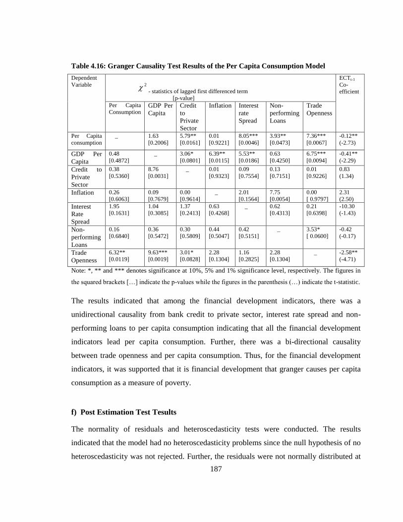
187
Table 4.16: Granger Causality Test Results of the Per Capita Consumption Model
Dependent
Variable
2- statistics of lagged first differenced term
[p-value]
ECTt-1
Co-
efficient
Per Capita
Consumption GDP Per
Capita
Credit
to
Private
Sector
Inflation Interest
rate
Spread
Non-
performing
Loans
Trade
Openness
Per Capita
consumption
_ 1.63
[0.2006]
5.79**
[0.0161]
0.01
[0.9221]
8.05***
[0.0046]
3.93**
[0.0473]
7.36***
[0.0067]
-0.12**
(-2.73)
GDP Per
Capita
0.48
[0.4872]
_ 3.06*
[0.0801]
6.39**
[0.0115]
5.53**
[0.0186]
0.63
[0.4250]
6.75***
[0.0094]
-0.41**
(-2.29)
Credit to
Private
Sector
0.38
[0.5360]
8.76
[0.0031]
_ 0.01
[0.9323]
0.09
[0.7554]
0.13
[0.7151]
0.01
[0.9226]
0.83
(1.34)
Inflation 0.26
[0.6063]
0.09
[0.7679]
0.00
[0.9614]
_ 2.01
[0.1564]
7.75
[0.0054]
0.00
[ 0.9797]
2.31
(2.50)
Interest
Rate
Spread
1.95
[0.1631]
1.04
[0.3085]
1.37
[0.2413]
0.63
[0.4268]
_ 0.62
[0.4313]
0.21
[0.6398]
-10.30
(-1.43)
Non-
performing
Loans
0.16
[0.6840]
0.36
[0.5472]
0.30
[0.5809]
0.44
[0.5047]
0.42
[0.5151]
_ 3.53*
[ 0.0600]
-0.42
(-0.17)
Trade
Openness
6.32**
[0.0119]
9.63***
[0.0019]
3.01*
[0.0828]
2.28
[0.1304]
1.16
[0.2825]
2.28
[0.1304]
_ -2.58**
(-4.71)
Note: *, ** and *** denotes significance at 10%, 5% and 1% significance level, respectively. The figures in
the squared brackets […] indicate the p-values while the figures in the parenthesis (…) indicate the t-statistic.
The results indicated that among the financial development indicators, there was a
unidirectional causality from bank credit to private sector, interest rate spread and non-
performing loans to per capita consumption indicating that all the financial development
indicators lead per capita consumption. Further, there was a bi-directional causality
between trade openness and per capita consumption. Thus, for the financial development
indicators, it was supported that it is financial development that granger causes per capita
consumption as a measure of poverty.
f) Post Estimation Test Tesults
The normality of residuals and heteroscedasticity tests were conducted. The results
indicated that the model had no heteroscedasticity problems since the null hypothesis of no
heteroscedasticity was not rejected. Further, the residuals were not normally distributed at
188
5 percent significance level since the null hypothesis of normality was rejected as the
probability value was 0.007. However, this was not a problem since the data set was
sufficient to produce unbiased estimates of the model (Refer to Table A:21 in appendix).
4.5 Conclusion and Policy Implications
The main objective of this chapter was to determine the effect of financial development on
poverty and establish the channels through which this effect takes place. The study used
several indicators of financial development including bank credit to private sector, interest
rate spread and non-performing loans. The study also used headcount ratio as well as per
capita consumption to determine this relationship. The study used the VECM to analyse
this relationship and several diagnostic tests were also carried out.
The findings showed that financial development was a contributor to poverty reduction.
The direct channel was supported by the financial development indicators whose
coefficients were significant. Credit to private sector was negatively related to poverty both
in the long run and in the short run. It also reduces poverty. Interest rate spread was
positively and significantly related to poverty implying that an increase in the interest rate
spread increases poverty. Non-performing loans were also bad for poverty in the short run.
High transaction costs and low quality of assets (an indication of inefficiency) increases
poverty. This was a new finding in the relationship between financial development and
poverty in Kenya. In addition, financial innovation was found to be negatively related with
poverty implying that introduction of new financial products among other innovations
helps in reducing poverty. This was a new finding indicating the importance of M-Pesa
financial innovation for poverty reduction.
The results also indicated that the indirect channel or the trickle down hypothesis of the
effect of financial development on poverty was present both in the long run and in the
short run. Growth leads to poverty reduction. On the causality relationships, economic
growth was found to granger cause poverty while credit to private sector and interest rate
189
spread as indicators of financial development were found to granger cause poverty.
Therefore, a one way causality was supported from financial development to poverty and
from economic growth to poverty.
The results using per capita consumption also supported the direct channel of the effect of
financial development on poverty. Interest rate spread and non-performing loans were
found to have a negative effect on per capita consumption in the long run. This was a
significant finding as it touches on the efficiency and quality of financial development.
Trade openness was also found to reduce poverty. On the granger causality results, only a
one way causality from financial development to per capita consumption was found thus
supporting the studies that indicate a one way causality from financial development to
poverty reduction. However, it was noted that there are enormous drawbacks of using per
capita consumption and the study relied on the results of the head count ratio model.
Findings indicated that financial development was important for poverty reduction.
Policies should be put in place to encourage the growth of the financial sector by the
government. This could be through encouraging use of technological innovations,
providing short term borrowing and others. Interest rate spread was negatively related with
poverty and had a signicant coefficient. The Central Bank ought to consider reduction of
the interest rate spread by coming up with interest rate policies that would raise the savings
rate since a wide interest rate spread is bad for poverty. These include tax exemption on
certain types of savings account and promoting the use of financial technological
innovations for saving. They may also consider setting an interest rate spread threshold
which financial institutions should not go beyond.
Non-performing loans were found to negatively impact poverty and the coefficient was
significant. Efficiency of the financial sector needs to be enhanced by ensuring proper
screening of customer loans, monitoring of credit as well as putting appropriate measures
for collateral by the financial institutions. The Central Bank should also ensure that proper

190
supervision of the financial institutions is maintained to deal with non-performing loans.
Non performing loans are not good for poverty since they form a vicious cycle of non-
performing loans and poverty.
The size of financial development as given by credit to private sector was important for
poverty since its coefficient was significant and negative. Therefore, policies to increase
the credit to private sector should be put in place by the government through the Central
Bank to ensure the government does not hinder this credit by borrowing too much and thus
crowding out the private sector. Further, financial institutions should ensure enabling
procedures for the private sector to access credit. The Central Bank should also ensure that
borrowing rates are not so exobitantly high that they block borrowers.
The coefficient of GDP Per Capita was significant and negative. It measured economic
growth and hence it was important for poverty reduction. Policies that promote growth
through innovations need to be put in place by the government. Policies that raise growth
such as an enabling macro economic environment need to be put in place too. Moreso,
policies to maintain low inflation by the Central Bank should also be formulated.
Furthermore, other factors that negatively affect growth like income inequality need to be
addressed and policy makers need to target a growth pattern that is more inclusive. Policies
like tax reforms and welfare transfers. In addition, it is important to invest in education and
development of skills to increase the employability of the population.
The significance of trade openness was shown with a significant and negative coefficient.
Policies should be set by the government to improve bilateral and multilateral trade. Export
promotion strategies ought to be introduced. Policies on value addition especially for
agricultural production ought to be enacted. Kenya should sign trade agreements which
promote affordable but beneficial trade.
191
Financial innovation was found to have a significant and negative coefficient. Hence, it
was important for reducing poverty. The government should not only support financial
innovation but also create a favourable environment for their growth. There should be
efforts by the government to give tax exemptions for financial innovations. Finally, the
Central Bank and the CCK ought to maintain a regulatory system whose flexibility allows
growth of financial innovations. This is important since the formal financial sector may not
fully meet the needs of the poor yet these innovations fill this gap.
4.6 Contribution of the Study
The study was important as it contributes to the finance – poverty nexus and fills the gap
that has not been addressed in Kenya. Since data on poverty is scarce, scholars have shied
away from country specific studies on financial development and poverty. This study was
useful in filling this gap. One of the main contributions was to determine whether the
direct or the indirect channels of financial development on poverty exist in Kenya. It used
appropriate indicators of financial development. Both the channels were supported from
the findings indicating the importance of financial development. It also contributed to
showing whether the quality of financial development affects poverty. Financial innovation
is on the move in Kenya. This study demonstrated how these innovations affect poverty.
Further, the consideration of structural breaks was important to show whether they
significantly change the results.
4.7 Limitations of the Study
The main limitation of the study was data scarcity. For example, data for financial
innovation was not available for the whole period of the study, 2000 to 2014. Poverty data
is wanting in all African countries and Kenya is not an exception. However, this data
limitation was addressed by using a dummy and also predicting quarterly poverty rates
using the decomposition method as explained in variable measurement. However, it is
believed that this data is reliable and policy recommendations can be made from the results
of the data.

192
4.8 Areas for Further Research
There is need to conduct thresholds effects especially for financial development indicators
so as to know the level at which financial development indicators affect poverty. This
would also be important for the control variables. Further research using other measures of
poverty which show the depth and severity of poverty for robustness are important. This is
because very little literature on this area exists and thus the relationship may not be fully
understood. Data may not be available at the moment but with the completion of the next
KIHBS in 2017, recent data would be available. Literature on financial sector inefficiency
and how it affects poverty is missing in Kenya hence there‘s need for further research to
shed light on this relationship.

193
CHAPTER FIVE
SUMMARY, CONCLUSIONS AND POLICY IMPLICATIONS
5.1 Introduction
This chapter concluded the thesis by a way of summarizing the study, giving conclusions
and policy implications. It also discussed the limitations of the study and areas of further
research. The contribution of the study to knowledge was also indicated.
5.2 Summary of the Thesis
The study addressed the debate on the relationship between financial development and
economic growth. It also addressed the relationship between financial development and
poverty which has been largely ignored. It started by determining the drivers of financial
development. The study incorporated financial innovations which have taken off. The main
objectives of the study were; to analyse the determinants of financial development; to
determine the effect of financial development on economic growth; and to determine the
effect of financial development on poverty.
The first chapter introduced financial developments and innovations in Kenya. This
chapter laid an important basis for the three essays in the thesis. The first essay (chapter
two) sought to determine the drivers of financial development in Kenya using the ARDL
model and quarterly data for the period 2000 to 2014.
Three hypotheses (economic institutions, endowment and openness hypothesis) were
tested and the results revealed two distinct findings. The credit to private sector model
supported the openness hypothesis that openness is important for financial development.
Conversely, the non-performing loans model supported the economic institutions and
endowment hypotheses which show that institutional quality is important for financial
development. These findings were as expected since trade would be important for the
194
quantitative side of financial development while institutional quality would be more
important for the qualitative and efficiency of financial development.
The level of financial development was also found to be driven by a number of other
factors. These factors included GDP per capita, democratic accountability, mobile
technology and inflation. Higher GDP per capita, less inflation, better democratic
accountability and more uptake of mobile technology were found to promote financial
development by increasing credit to private sector and reducing non-performing loans. The
results of the market capitalization model were weak since the results indicated that there
was no long-run relationship between market capitalization and its determinants.
The second essay‘s (chapter three) main objective was to determine the relationship
between financial development and economic growth while using efficiency measures as
well as controlling for financial innovation. The essay utilized cointegration analysis,
granger causality, Vector Error Correction Model as well as the variance decomposition in
determining this relationship. Quarterly data for the period 2000 to 2014 was used for all
the variables obtained from CBK, NSE, KNBS and WDI.
The findings indicated that financial development was important for economic growth.
Interest rate spread, non-performing loans and credit to private sector were negatively
related with economic growth while market capitalization influences economic growth
positively. On causality, the supply leading hypothesis was found to be predominant.
Credit to private sector and economic growth had a bi-directional relationship. The choice
of financial development indicator is therefore important for determining the causality
between financial development and economic growth. The new finding indicated the
importance of the quality and efficiency of the financial sector growth for economic
growth. Further, financial innovation was significant and influences economic growth
positively. This is a new contribution for policy makers and researchers in establishing the
relationship between financial development and economic growth.

195
The third essay (chapter four) sought to determine the effect of financial development on
poverty in Kenya. It introduced the use of efficiency measures of financial development as
well as controlled for financial innovation. The study used cointegration analysis, granger
causality and Vector Error Correction Model to determine this relationship. Quarterly data
for the period 2000 to 2014 was used for all the variables obtained from CBK, KNBS and
WDI. Head count ratio was predicted using the (poverty changes) decomposition method.
The VECM results indicated that the indirect channel or the trickle down hypothesis of the
effect of financial development on poverty through economic growth was present while
using head count ratio. The direct channel was also supported by the financial development
indicators. Credit to private sector was negatively related to poverty both in the long and
short run while interest rate spread and non-performing loans were positively related with
head count ratio implying they increase poverty. Financial innovation, in specific M-Pesa
was found to be important for poverty reduction.
On the causality relationships, economic growth was found to granger cause poverty
reduction while credit to private sector and interest rate spread were found to granger cause
poverty. Thus, a one way causality was supported from financial development to poverty
and from economic growth to poverty. Trade openness was also found to have a positive
impact on poverty in the long run. Further analysis using per capita consumption supported
the direct effect of financial development on poverty reduction.
5.3 Conclusions
The objectives of the study were to determine the drivers of financial development, as well
as determine the effect of financial development on economic growth and povery. This was
done using the ARDL model, the VECM, cointegration analsysis and granger causality.
The study had three main conclusions. One, financial development is dependent on
economic growth, institutional quality, trade openness, democratic accountability, inflation
and mobile technology depending on the indicator of financial development used. It helped
create an understanding of why Kenya is at its current level of financial development. Two,
196
financial development influences economic growth positively and the supply leading
hypothesis is predominant in Kenya. Three, financial development reduces poverty both
through the direct channel and the indirect channel through economic growth. It was clear
that the quality and efficiency of the financial sector are important for both economic
growth and poverty reduction. Furthermore, financial innovation is important for
improving economic growth and for poverty reduction.
It is therefore inherent that both the financial and the real sectors are important in Kenya.
Moreso, the quality and efficiency aspects of financial development are important for
growth and poverty reduction. The study thus met the three objectives which were set out
at the beginning and also made a contribution to literature and policy in Kenya.
5.4 Policy Implications
Institutional quality was found to be a significant determinant of financial development
since the coefficient was significant. Policies that improve the institutional environment in
the financial sector should be pursued by the government, the Central Bank and financial
institutions. The government should ensure proper functioning of legal and regulatory
institutions to guarantee protection of property rights and enforcement of credit contracts.
There is also need to enforce anti corruption policies so as to enhance transparency and
accountability in business transactions. More credit reference bureaus should be
established to reduce default on credit.
Trade was a driver of financial development and it was found to be significantly and
positively related to financial development. Policies should be directed at the long term
benefits of trade since the effect was in the long term. The government should formulate
more export promotion strategies. This would require policies to increase value addition
especially for primary agricultural products. There should also be efforts to reduce imports
of financially dependent goods and services.
197
Both GDP per capita and inflation were found to have significant coefficients and were
important determinants of financial development. GDP per capita was positively related
while inflation was negatively related with financial development. Based against this
background, policies to ensure a good macro-economic environment are important. Growth
of the real economy is important as it increases the GDP per capita of individuals.
Strengthening legal and other institutions, maintaining a good macro environment and
improving human capital development are some of the policies which can ensure continued
growth in GDP per capita. Policies to maintain inflation at threshold levels such as
inflation targeting should be pursued by the Central Bank.
The political economy is important for financial development as it promotes well
functioning economic institutions. This was derived from the findings where the
democratic accountability coefficient was significant and positive. The government should
come up with laws and policies which enhance democratic space and create a conducive
political environment. So far, the new Kenyan Constitution of 2010 has been important in
enhancing democracy and decentralizing power through devolution. Other policies include
a system of political checks and balances, an increase in citizens‘ voice, increased
accountability, increased individual rights and reduced influence by interest groups.
Mobile technology also promotes financial development as shown through the significant
and positive coefficient. The government should create a conducive environment for
mobile phone innovations. Policies aimed at increasing the use of mobile technology in the
financial sector should be encouraged. So far, Kenya is leading in the use of mobile money
through M-Pesa and such innovations should be encouraged to tap fully into the benefits of
technology. Such policies include licensing and tax exemptions for new innovations in
mobile technology use. The CBK has so far ensured an enabling environment for banks to
work with Safaricom Ltd and other MNOs in advancing the use of mobile banking.

198
Based on the conclusions that the Mckinnon hypothesis prevails, it is important for the
policy makers to support the growth of the financial sector. Non-performing loans had a
significant coefficient and negatively affected economic growth and poverty. Efficiency
and quality in the financial sector especially in the banking sector needs to be enhanced.
Increase in non-performing loans was found to be detrimental to the poor and to economic
growth. The banking sector needs to address the inefficiency leaks such as the non-
performing loans by increasing screening of borrowers at the onset. Proper monitoring of
loan repayments as well as obtaining proper collateral for the loans need to be adhered to.
Competition in the banking industry may have led to laxity in the lending processes. For
example, laxity in the Know Your Customer requirements. The Central Bank ought to
ensure that lending and other banking procedures are followed. It should also ensure that
credit reference bureaus are operational and sufficient to handle defaulters.
Interest rate spread was found to be significant and having a negative effect on economic
growth and poverty. Financial sector reforms should be undertaken including interest rate
reforms by the Central bank of Kenya to reduce the interest rate spread which impacts
negatively on the poor possibly by setting interest rate ceilings on lending rates or setting
certain thresholds for interest rate spread. In addition, policies that would raise the savings
rate need to be encouraged like setting higher Treasury Bill rates by the Central Bank.
Once the gap or spread between deposit and lending rates is reduced, then there can be
more efficient allocation of resources to the most productive sectors.
The coefficient of credit to private sector was significant and negative, implying that credit
to private sector was detrimental to economic growth. This may be due to wastage and
inefficiencies. Thus, financial institutions, the Central Bank and the government ought to
ensure proper monitoring, evaluation and supervision of these funds as well as proper
supervision of the financial sector by the Central Bank. This would curtail credit wastage
especially during years when the country undergoes a general election. In regards to the
poverty model, the coefficient was negative and significant. For this reason, policies to

199
increase the credit to private sector should be put in place by the CBK to ensure that the
government does not crowd out the private sector. This may pinch-hit the benefits gained
by the private sector where resource allocation is more competitive. In addition, financial
institutions should ensure an enabling environment for the private sector to access credit.
The Central Bank should also ensure that borrowing rates are not too high. Thus, policies
to maintain favorable interest rates should be considered.
Stock market development was found to be important for economic growth since the
coefficient of market capitalization was significant and positive. Hence, it is important that
a conducive environment prevails in the stock market. This would enable increased
company listing and their ability to acess long term finance. Low corporate tax and foreign
participation policies should be put in place by the government. These would ensure that
more corporate organizations use this form of funding and list at the stock exchange.
Moreover, financial innovations were found to positively impact on poverty reduction and
economic growth. The coefficient was significant and positive on economic growth and
negative on poverty. The growth of M-Pesa and other forms of innovations in Kenya
should be supported by all stakeholders since they lead to increased access to financial
services especially by the poor. A stable regulatory (institutional and legal) framework
between the CBK and the CCK need to always exist to regulate M-Pesa and other
innovations. This would ensure fraud issues are taken care of and users continue to
appreciate the product. Further, a conducive environment needs to exist for both financial
institutions and non-financial institutions to tap onto benefits of M-Pesa and other financial
innovations. The Central Bank should also have flexible but vigilant regulations so as to
allow other financial innovations which are beneficial to the economy. The government
may support financial innovations through tax exemption policies, capital availability and
structural reviews.
200
In addition, the findings indicated that economic growth was important for poverty
reduction since the coefficient was significant and negative. Hence, the government should
come up with policies which promote growth through innovations (like M-Pesa). Further,
other policies which promote economic growth need to be put in place, for example
policies like inflation targeting to maintain a good macro economic environment.
Furthermore, the government should invest in education and human resource development.
This makes citizens more professionally productive and useful to economic growth.
Trade openness was important for both economic growth and poverty with a positive and
negative significant coefficient on economic growth and poverty respectively. The
government should ensure trade policies focusing on trade agreements, both bilateral and
multilateral to increase trade in Kenya. However, the benefits from trade to poverty are not
spontaneous; but rather work together with other policies icluding good financial sector
reforms like liberalization and prudential supervision, investments in human resource
capacity as well as improved governance. Thus, government policy makers in trying to
improve the trade conditions in Kenya should also formulate policies that grow the
financial sector to ensure the positive effects of trade openness are sustained.
5.4 Contribution of the Study to Knowledge
The study contributes new knowledge to the finance-growth nexus. It deviates from
existing studies in Kenya by incorporating the quality of the financial sector which has
been left out in the Kenyan literature. Use of variables like non-performing loans and
interest rate spread is vital as they take into account the quality of financial development;
not just the quantity. It also contributes further to the debate on finance and growth in
Kenya by incorporating the financial innovation aspect of financial development to show
how financial innovation affects economic growth as well as poverty. Financial innovation
increases economic growth while reducing poverty. From literature, there are conflicting
findings on the nature of causality and this study is instrumental in contributing to this lack
of clarity. The study findings conclude that this lack of clarity can only be settled when we
201
incorporate multi-dimensional aspects of financial development including quality and
efficiency and not just the quantitative aspects of financial development. Incorporating
these aspects, then the supply leading hypothesis is pre-dominant.
The study also contributes new knowledge on why the level of financial development is at
its current level by determining what drives financial development. Institutional quality is
important for the quality of financial development while more openness is key for
quantitative financial development. These are key for policy and literature. The
relationship between financial development and poverty has been ignored in Kenya and
this study comes in to shed light on this relationship. It shows that both the indirect and
direct channels of the effect of financial development on poverty reduction are evident.
Furthermore, ignoring the presence of structural breaks could lead to wrong inferences and
wrong results. It may even be the reason for the mixed results on the relationship between
financial development and growth. This is a worthy contribution on the impact of
structural breaks.
5.5 Limitations of the Study
The main limitation was data scarcity. Some of the data sets were not available on a
quarterly basis, hence there was need to convert annual to quarterly data. On financial
innovations, in our case, M-Pesa volumes, the data only dates back to the year 2007 when
M-Pesa was introduced and hence the reason for the use of a dummy. Time series data on
poverty was scarce and hence the study chose to predict quarterly poverty rates using the
decomposition method. The study could not capture financial openness also due to scarcity
of data. However, the results of the study were reliable as it is believed that the data used
certainly provide credible information for giving policy recommendations on the
relationship between financial development, growth and poverty.
202
5.6 Areas for further research
There is need to consider threshold effects of financial development so as to determine at
which levels (based on financial development indicators), financial development is
important for economic growth and poverty. This is also important for classifying
countries that are more financially developed from those that are less financially
developed. Research on how innovations affect not just economic growth and poverty but
other macroeconomic variables like unemployment is important. This is possible with
availability of actual data. In addition, more research on financial sector efficiency and
how it affects poverty is important in Kenya since this literature is lacking. Finally, it
would be important to check for robustness to different measures of poverty including
poverty gap, poverty gap squared and severity dimensions of poverty and how they are
affected by financial sector developments and innovations. Other robustness checks would
include robustness to different estimation methods to validate the findings.

203
REFERENCES
Abraham, T. W. (2015), ―Financial Innovation and Poverty Reduction: Evidence from
Rural Northern Nigeria‖, MFW4A Working Paper No. 1, July 2015.
Available at: http://www.mfw4a.org/; accessed: 6.2.2016
Abzari, M., Zarei, F. and Esfahani, S. S. (2011), ―Analyzing the Link between Financial
Development and Foreign Direct Investment among D-8 Group of
Countries‖. International Journal of Economics and Finance 3(6): 148-
156
Acemoglu, D., Johnson, S. and Robinson, J. A. (2001), ―The Colonial Origins of
Comparative Development: An Empirical Investigation‖. American
Economic Review 91: 1369 – 1401
Acemoglu, D., Johnson, S. and Robinson, J. A. (2004), ―Institutions as the Fundamental
Cause of Long-Run Growth‖, NBER Working Paper 10481
Adams, R. and Page, J. (2005), ―International Migration, Remittances and Poverty in
Developing Countries,‖ World Bank Policy Research Working Paper
3179
Adamopoulos, A. (2010), ―Financial Development and Economic Growth: A comparative
study between 15 European Union member-states‖, International
Research Journal of Finance and Economics, 35: 144-149.
Adnan, N. (2011), ―Measurement of Financial Development: A Fresh Approach‖, 8th
International Conference on Islamic Economics and Finance, UK
Aduda J., Masila, J. and Onsongo, E. (2012), ―The Determinants of Stock Market
Development: The Case for the Nairobi Stock‖, International Journal of
Humanities and Social Science 2: 214-230
Agbetsiafa, D. K. (2003), ―The Finance Growth Nexus: Evidence from sub-Saharan
Africa‖, International Advances in Economic Research 9(2): 271-288

204
Aggarwal, R., Demirguc-Kunt A. and Peria, M. S. M. (2006), ―Do Workers' Remittances
Promote Financial Development?‖ World Bank Policy Working Paper
No. 3957
Aggarwal, R., Demirguc-Kunt A. and Peria, M. S. M. (2011), ―Do Remittances Promote
Financial Development?‖ Journal of Development Economics 96(2):
255-264
Aghion, P. and Bolton, P. (1997), ―A theory of trickle-down theory and development‖, The
Review of Economic Studies 64(2): 151-172
Aizenman, J. (2004), ―Financial Opening and Development: Evidence and Policy
Controversies‖, American Economic Review 94(2): 65-70
Aizenman, J. and Noy, I. (2006), ―Endogenous Financial and Trade Openness: Efficiency
and Political Economy Considerations‖, NBER Working Paper 2004/04
Aker, J. C. (2010). ―Information from Markets Near and Far: The Impact of Mobile
Phones on Agricultural Markets in Niger‖, American Economic
Journal: Applied Economics 2: 46–59
Akinboade, O.A. (1998), ―Financial Development and Economic Growth in Botswana: A
Test for Causality‖, Savings and Development 22(3): 331-348.
Akinlo, A. E. and Egbetunde, T. (2010), ―Financial Development and Economic growth:
The Experience of 10 Sub-Saharan African countries Revisited‖, The
Review of Finance and Banking, 2 (1): 17-28.
Akosah, N. K. (2013), ―Dynamics of Inflation and Financial Development: Empirical
Evidence from Ghana‖. Journal of Economics and Sustainable
Development 4: 20-37
Ali, A. and Thorbecke, E. (2000), ―The State and Path of Poverty in Sub-Saharan Africa‖,
Journal of African Economies 9(1): 1–40.
Allaro, H. B., Kassa, B. and Hundie, B. (2011), ―A Time Series Analysis of Structural
Break Time in the Macroeconomic Variables in Ethiopia‖, African
Journal of Agricultural Research 6(2): 392-400

205
Al-Nasser, O. and Jackson, D. (2012), ―The Impact of Financial Sector Performance in
Latin American Countries‖. University of Texas-Pan American,
Edinburg
Alter, A. and Yontcheva, B. (2015), ―Financial Inclusion and Development in the
CEMAC‖. IMF Working Paper No. WP/15/235
Amanja, D. and Morrissey, O. (2005), ―Fiscal Policy and Economic Growth in Kenya‖.
Credit Research Paper No. 05/06. June, 2005. Available at:
http://www.nottingham.ac.uk/credit/documents/papers/05-06.pdf.
accessed: 16.10.2013
Ang, J.B. and McKibbin, W. J. (2007), "Financial Liberalization, Financial Sector
Development and Growth: Evidence from Malaysia," Journal of
Development Economics, 84(1): 215-233
Antzoulatos, A., Kyriazis, D. and Tsoumas, C. (2008), "Financial Development and
Asymmetric Information‖. MPRA Paper No. 23013
Arcand, J., Berkes, E. and Panizza, U. (2012), ―Too Much Finance?‖ International
Monetary Fund, Working Paper 12:161
Arestis, P. and Demetriades, P. (1997), ―Financial Development and Economic Growth:
Assessing the Evidence‖. The Economic Journal 107: 783-799.
Arestis, P., Demetriades, P. and Luintel, K. B. (2001), ―Financial Development and
Economic Growth: The Role of Stock Markets‖ Journal of Money,
Credit and Banking 33(1): 16-41.
Athukorala, P. and Sen, K. (2005). ―Saving, Investment and Growth in India‖, Economic
Development and Cultural Change 52(4):896-900
Avais, M. (2014), ―Financial Innovation and Poverty Reduction‖, International Journal of
Scientific and Research Publications 4(1): 2250-3153
Ayadi, R., Arbak, E., Naceur, S. B. and De Groen, W. P. (2013), ―Determinants of
Financial Development Across the Mediterranean‖ MEDPRO Working
Paper No. 29
206
Aye, G. C. (2013), ―Causality between Financial Deepening, Economic Growth and
Poverty in Nigeria‖, The business and Management Review 3(3): 1-11
Bakhtiari, S. (2006), ―Microfinance and Poverty Reduction: Some International Evidence‖,
International Business & Economics Research Journal 5(12): 65-71
Baliamoune-Lutz, M. (2008). ―Financial Development and Income in North Africa‖.
International Advances in Economic Research, 14(4): 422-432.
Baltagi, B. H., Demetriades, P. and Law, S. H. (2009), ―Financial Development and
Openness: Evidence from Panel Data‖ Journal of Development
Economics 89: 285-296
Baltagi, B. H., Demetriades, P. and Law, S. H. (2007), ―Financial Development, Openness
and Institutions: Evidence from Panel Data‖. Conference on New
Perspectives on Financial Globalization. Washington D.C
Bayoumi, T. (1990), ―Financial Innovation and Consumption in the United Kingdom, IMF
Working Paper No. WP/90/95.
Beccalli, E. (2007), ―Does IT Investment Improve Bank Performance? Evidence from
Europe‖. Journal of Banking and Finance 31(7): 2205–2230.
Becerra, O., Cavallo, E. and Scartascini, C. (2012), ―The Politics of Financial
Development: The Role of Interest Groups and Government
Capabilities‖. Journal of Banking and Finance 36: 626–643
Beck, T. (2002), ―Financial development and international trade: is there a link?‖ Journal
of International Economics, 57: 107-131
Beck, T., Levine, R. and Loayza, N. (2000), ―Finance and the sources of growth‖, Journal
of Financial Economics 58(1-2): 261-300
Beck, T., Demirgüç-Kunt, A. and Levine, R. (2001) ―The Financial Structure Database,‖ in
A. Demirguc-Kunt and R. Levine (eds.) Financial Structure and
Economic Growth: A Cross-Country Comparison of Banks, Markets,
and Development, Cambridge, MA, The MIT Press.
Beck, T., Fuchs, M., Singer, D. and Witte, M. (2014), ―Making cross-border banking work
for Africa‖. Technical report, The World Bank/KfW
207
Beji, S. (2007), ―Financial Openness and Financial Development in the South
Mediterranean Sea Countries: Institutional Approach and Calculation of
Development Thresholds‖. European Research Studies 11: 107-127.
Bencivenga, V. R. and Smith, B. D. (1992), ―Deficits, inflation and the banking system in
developing countries: The optimal degree of financial repression‖.
Oxford Economic 44: 767-790
Bencivenga, V. R. and Smith, B. D. (1991), ―Financial Intermediation and Endogenous
Growth‖, The Review of Economic studies, 58: 195-209.
Ben-David, D. and Papell, D.H. (1995), ―The Great Wars, the Great Crash and the Unit
Root Hypothesis‖, Journal of Monetary Economics 36: 453-475.
Berger, A. N. (2003), ―The Economic Effects of Technological Progress: Evidence from
the Banking Industry‖. Journal of Money, Credit and Banking 35(2):
141–176
Bittencourt, M. (2008), ―Inflation and Financial Development: Evidence from Brazil‖,
UNU-WIDER, Research Paper No. 2008/14
Blach, J. (2011), ―Financial Innovations and their Role in the Modern Financial System –
Identification and Systematization of the Problem‖, Financial Internet
Quarterly, e-Finanse 7(3): 13-26
Bleaney, M. F. (1996), ―Macroeconomic Stability, Investment and Growth in Developing
Countries‖. Journal of Development Economics 48: 461–477
Boudriga, A., Taktak, N. B. and Jellouli, S. (2010), ―Problem Loans in the MENA
Countries: Bank Specific Determinants and the Role of the Business and
the Institutional Environment‖. Economic Research Forum, Working
Paper No. 547
Boudriga, A., Taktak, N. B. and Jellouli, S. (2009), ―Banking Supervision and Non-
performing Loans: A Cross Country Analysis‖. Journal of Financial
Economic Policy 1(1): 286-318
Boyd, J. H., Smith, B. D. and Levine, R. (2001), ―The Impact of Inflation on Financial
Sector Performance‖. Journal of Monetary Economics 47: 221-248.

208
Boyd, J. H., Smith, B. D. and Levine, R. (1996), ―Inflation and Financial Market
Performance‖. Pennsylvania State University
Brown, R. P., Carmignani F. and Fayad G. (2011), ―Migrants‘ Remittances and Financial
Development: Macro- and Micro-level Evidence of a Perverse
Relationship‖. Department of Economics, OxCarre Research Paper 59
Buku, M. and Meredith, M. (2013), ―Safaricom and M-Pesa in Kenya: Financial Inclusion
and Financial Integrity‖ Washington Journal of Law, Technology &
Arts, 8(3): 376-400
Calderon, C. and Lin, L. (2003), ―The Direction of Causality between Financial
Development and Economic Growth‖, Journal of Development
Economics 72: 321-334.
Camillo, A. (2015), ―Handbook of Research on Global Hospitality and Tourism
Management‖ Woodbury University, USA
Capital Markets Authority (2013), Annual Report, 2013. Nairobi, Capital Markets Authority.
Caporale, G. M., Rault, C., Sova, R. and Sova, A. (2009), ―Financial Development and
Economic Growth: Evidence from Ten New EU Members‖, Discussion
paper 940, German Institute of Economic Research, Berlin.
Central Bank of Kenya (2015), ―Annual Report: July 2014- June 2015‖. Nairobi: Central
Bank of Kenya
Central Bank of Kenya (2014a), Bank Supervision Annual Report, Annual Report: July
2013- June 2014‖. Nairobi: Government Printers
Central Bank of Kenya (2014b), ―Annual Report: July 2013- June 2014‖. Nairobi: Central
Bank of Kenya
Central Bank of Kenya (2013a), Annual Report, 2013. Nairobi, Central Bank of Kenya.
Central Bank of Kenya (2013b), Statistical Bulletin, March 2013, Nairobi, Central Bank of
Kenya.
Central Bank of Kenya (2012), ―Annual Report: July 2011- June 2012‖. Nairobi: Central
Bank of Kenya

209
Central Bank of Kenya (2010), Annual Report: July 2009- June 2010‖. Nairobi:
Government Printers
Central Bank of Kenya (2009), Annual Report: July 2008- June 2009‖. Nairobi:
Government Printers
Chen, P. and Gupta, R. (2006), ―An Investigation of Openness and Economic Growth
using Panel Estimation‖, University of Pretoria, Working Paper No.
2006-22.
Chhibber, A. and Nayyar, G. (2007), ―Pro-Poor Growth: Explaining the Cross-Country
Variation in the Growth Elasticity of Poverty‖, BWPI Working Paper
14, The World Bank.
Chinn, M. D. and Ito, H. (2006), ―What matters for Financial Development? Capital
Controls, Institutions and Interactions? Escholarship, University of
California
Cho, Y. (1986), ―Inefficiencies from Financial Liberalization in the Absence of Well-
Functioning Equity Markets‖, Journal of Money, Credit & Banking, 18:
191-199.
Chowdhury, M. B. (2011), ―Remittances Flow and Financial Development in Bangladesh‖,
Economic Modelling 28: 2600-2608
Christiaensen, L., Demery, L. and Paternostra, S. (2003), ―Macro and Micro Perspectives
of Growth and Poverty in Africa‖, The World Bank Economic Review,
17(3): 17-347
Chuah, H. L. and Thai, V. (2004), ―Financial Development and Economic Growth:
Evidence from Causality Tests for the GCC Countries‖, IMF Working
Paper, WP/04/XX.
Chukwu, J. O. and Agu, C. C. (2009), ―Multivariate Causality between Financial Depth
and Economic Growth in Nigeria‖. African Review of Money Finance
and Banking 7-21
Clemente, J., Montanes, A. and Reyes, M. (1998). ―Testing for a unit root in variables with
a double change in the mean‖, Economics Letters 59: 175-182.
210
Commercial Bank of Africa (2014), ―Annual Report: January – December 2014‖. Nairobi:
Commercial Bank of Africa
Communications Authority of Kenya (2014), ―Sector Statistics Report‖. Nairobi:
Communications Authority of Kenya
Communications Authority of Kenya (2012), ―Sector Statistics Report‖. Nairobi:
Communications Authority of Kenya
Crichton, N. and De Silva, C. (1989), ―Financial Development and Economic Growth:
Trinidad and Tobago, 1973-1987‖, Social and Economic Studies 38 (4):
133-162.
Curak, M., Pepur, S. and Poposki, K. (2013), ―Determinants of Non-performing Loans:
Evidence from South-eastern European Banking Systems‖. Banks and
Bank Systems 8(1): 45-53
Dabla – Norris, E., Ji, Y., Townsend, R. M. and Unsal, D. F. (2014), ―Financial
Deepening, Growth, and Inequality: A Structural Framework for
Developing Countries‖, International Monetary Fund
D‘alfonso, E. and Moretti, L. (2012), ―The finance-growth nexus in CEE: New evidence
from a survey-based indicator of external finance dependence‖,
Economics Bulletin 32(3): 2688-2699
Dandume, M. Y. (2014), ―Financial Sector Development, Economic Growth and Poverty
Reduction: New Evidence from Nigeria‖, Journal of the Faculty of
Economics Fakültesi Dergisi and Administrative Sciences 4(2): 1-20
Dauda, R. O and Makinde, K. O. (2014), ―Financial Sector Development and Poverty
Reduction in Nigeria: A Vector Autoregression Analysis (1980-2010)‖,
Asian Economic and Financial Review 4(8): 1040-1061
Dekle, P. and Pundit, M. (2015), ―The Recent Convergence of Financial Development in
Asia‖ ADB Economics Working Paper Series No. 440
Dembiermont, C., Drehmann, M. and Muksakunratana, S. (2013), ―How much does the
private sector really borrow? A new database for total credit to the
211
private nonfinancial sector‖, BIS Quarterly Review 65-81. Available at:
http://www.bis.org/publ/qtrpdf/r_qt1303h.pdf.
Demetriades, P. O. and Andrianova, S. (2005), ―Sources and Effectiveness of Financial
Development: What We Know and What We Need to Know.‖ UNU –
WIDER World Institute for Development Economic Research Working
Papers RP2005/76
Demetriades, P. O. and Law, S. H. (2006), ―Openness, Institutions and Financial
Development.‖ WEF Working Papers 0012
Demetriades, P. and Hussein, K. (1996), ―Does Financial Development Cause Economic
Growth? Time Series Evidence from 16 Countries‖, Journal of
Development Economics 51: 387-411.
Demirgüç-Kunt, A., López Córdova, E., Martínez Pería, M. S. and Woodruff, C. (2011),
―Remittances and Banking Sector Breadth and Depth: Evidence from
Mexico‖. Journal of Development Economics 95(2): 229-241.
Devarajan, S. (2013), ―Africa's Statistical Tragedy‖, Review of Income and Wealth,
59: S9–S15
DFID (2004), ―The Importance of Financial Sector Development for Growth and Poverty
Reduction‖, Policy Division Working Paper. Available at:
http://purl.umn.edu/12886; accessed: 18.9.2015
Dhrifi, A. (2013), ―Financial Development and Poverty: What Role for Growth and
inequality?‖, International journal of Academic Research in
Accounting, Finance and Management Science 3(4), 119-129
Dickey, D.A. and Fuller, W. A. (1979), ‖Distribution of the Estimators for Autoregressive
Time Series with a Unit Root‖, Journal of the American Statistical
Association, 74: 427—431.
Djankov, S., McLiesh, C. and Shleifer, A. (2007), ―Private credit in 129 countries‖,
Journal of Financial Economics, 84(2): 299-329
Do, Q. and Levchenko, A. A. (2004), ―Trade and financial development‖, The World Bank
Working Paper, No. 3347

212
Dollar, D. and Kraay, A. (2002), ―Growth is good for the poor‖, Journal of Economic
Growth, 7:195-225
Duasa, J. (2006), ―Determinants of Malaysian Trade Balance: An ARDL Bound Testing
Approach‖. 6th
Global Conference on Business and Economics, USA
Dudian, M. and Popa, R. A. (2013), ―Financial Development and Economic Growth in
Central and Eastern Europe‖, Theoretical and Applied Economics,
8(585): 59-68.
Dushku, E. (2010), ―Financial Development and Economic Growth: The Albanian Case‖
Discussion Paper, Bank of Albania
Easterly, W. and Levine, R. (1997), ―Africa‘s Growth Tragedy: Policies and Ethnic
Divisions‖. Quarterly Journal of Economics 112:1203–1250.
Easterly, W. and Levine, R. (1994), ―Africa‘s growth tragedy‖. Paper presented at the
African Economic Research Consortium (AERC) workshop. Nairobi,
Kenya, May.
Easterly, W. and Fischer, S. (2001), ―Inflation and the Poor‖, Journal of Money, Credit,
and Banking 33(2): 160-178.
Effiong, E. L. (2015), ―Financial Development, Institutions and Economic Growth:
Evidence from Sub-Saharan Africa. MPRA Paper No. 66085
Elbadawa, I. A. and Ndulu, B. (1994), ―Long-term Development and Sustainable Growth
in Sub-Saharan Africa‖, Mimeo, African Economic Research
consortium (AERC)
Engle, R.F. and Granger, C. J. (1987), ―Cointegration and Error-correction -
Representation, Estimation and Testing‖, Econometrica 55 (2): 251-78.
English, B. W. (1999), ―Inflation and Financial Sector Size‖. Journal of Monetary
Economics 44: 379-400
Erosy, I. (2011), ―The Impact of Financial Openness on Financial Development, Growth,
and Volatility in Turkey: Evidence from the ARDL Bounds Tests‖.
Ekonomska Istrazivanja 24(3): 33-44

213
Esso, L. J. (2010), ―Re-examining the Finance-Growth Nexus: Structural Break, Threshold
Cointegration and Causality Evidence from the Ecowas‖. Journal of
Economic Development 35(3): 57-79
Fawcett, A. J. (2007), ―Principles of Assessment and Outcome Measurement for
Occupational Therapists and Physiotherapists: Theory, Skills and
Application‖. London: John Wiley and Sons Ltd.
Fernandez, A. and Tamayo, C. E. (2015), ―From Institutions to Financial Development and
Growth: What are the Links?‖ Journal of Economic Surveys, 29(1): 1-
41
Financial Sector Deepening Kenya (FSD), Central Bank of Kenya and Kenya National
Bureau of Statistics, (2016), ―The 2016 FinAccess Household Survey
infographics sheet‖. Nairobi, Kenya: FSD Kenya.
Financial Sector Deepening Kenya (FSD), Central Bank of Kenya and Kenya National
Bureau of Statistics (2013), ―FinAccess National Survey: Profiling
developments in financial access and usage in Kenya‖. Nairobi, FSD
Kenya.
Financial Sector Deepening Kenya (FSD), Central Bank of Kenya and Kenya National
Bureau of Statistics (2009), ―FinAccess National Survey: Dynamics of
Kenya‘s Changing Financial Landscape‖. Nairobi, FSD Kenya.
FitzGerald, V. (2006) ―Financial Development and Economic Growth: A Critical View‖.
Department of International Development (QEH), Working Paper No.
153.
Fording, R. and Berry, W. (2007), ―The Historical Impact of Welfare Programs on
Poverty: Evidence from the American States‖, The Policy Studies
Journal 35(1): 37-60.
Fowowe, B. and Abidoye, B. (2010) ―A Quantitative Assessment of the Effect of Financial
Development on Poverty in African Countries‖, Iowa State University
and University of Ibadan

214
Galor, O. and Tsiddon, D. (1997), ―The Distribution of Human Capital and Economic
Growth‖, Journal of Economic Growth 2: 93-12
Gautam, B. P. (2014), ―Financial Development and Economic Growth in Nepal‖. NRB
Working Paper No. 25, December 2014, Rastra, Nepal
Gehringer, A. (2013), ―Financial Liberalization, Financial Development and Productivity
Growth – An Overview‖, Economics Discussion Papers, No 2013- 46,
Kiel Institute for the World Economy
Ghatak, S. and Siddiki, J. (1999), ―Financial Liberalisation and Endogenous Growth: The
case of Bangladesh‖, Kingston University, School of Economics
Working Paper, London, UK
Ghosh, A. and Steven, P. (1998), ―Inflation, Disinflation and Growth,‖ IMF Working
Paper, Washington
Gichuhi, M. M. (2013), ―The role of financial systems in the Kenyan economy Challenges
and possible interventions (A theoretical review)‖, Prime Journal of
Business Administration and Management 3(10): 1197-1201
Giles, J.A. and Williams, C. L. (2000), ―Export-led Growth: A Survey of the Empirical
Literature and Some Non-causality Results: Part 1‖ Journal of
International Trade and Economic Development 9: 261–337.
Ginebri, S., Petrioli, G. and Sabani, L. (2001), ―Financial Deepening, Trade Openness and
Growth: A Multivariate Cointegrated Analysis of the Complementary
Effects‖, CIDEI Working Paper No.62, Rome, Italy.
Girma, S. and Shortland, A. (2008), ―The Political Economy of Financial Development‖.
Oxford Economic Papers 60(4): 567-596
Githaiga, P. N. and Kabiru, C. G. (2014), ―Remittances as a Determinant of Financial
Sector Development‖. Journal of Business, Economics and Finance
3(4): 398-424
Giuliano, P. and Ruiz-Arranz, M. (2006), ―Remittances, Financial Development and
Growth‖.IZA discussion Paper No. 2160, Institute for the Study of
Labour (IZA).

215
Graff, M. and Karmann, A. (2003), ‗‗What Determines the Finance-growth Nexus? An
Endogenous Growth Model and Empirical Evidence‘‘, Dresden
Discussion Papers in Economics 15/03.
Granger, C. W. (1988) ―Some Recent Developments in a Concept of Causality‖, Journal of
Econometrics, 39: 199-211.
Green, C. J. Kirkpatrick, C. H. and Murinde, V., (2006) ―Finance for Small Enterprise
Growth and Poverty Reduction inDeveloping Countries‖, Journal of
International Development, 18: 1017-1030.
Greiner, A., Semmler, W. and Gong, G. (2004), ―The Forces of Economic Growth: A
Time Series Perspective‖, Princeton University Press, Princeton
Gries, T. and Meierrieksy, D. (2010), ―Institutional Quality and Financial Development in
Sub- Saharan Africa‖. CSAE Conference: Economic Development in
Africa. Oxford
Grossman, G., and Helpman, E., (1990), ―Trade, Innovation and Growth‖, The American
Economic Review, 80: 86-91.
Gujarati D. N. and Porter, D. C. (2009), ―Basic Econometrics‖. Boston, Mass: McGraw-
Hill
Habibullah, M. S. and End, Y. (2006), ―Does Financial Development Cause Economic
Growth? A Panel Data Dynamic Analysis for the Asian Developing
Countries‖, Journal of the Asia Pacific Economy, 11(4): 377-393.
Harris, R. and Sollis, R. (2003), ―Applied Time Series Modelling and Forecasting‖, John
Wiley, New York
Harrison, P., Sussman, O. and Zeira, J. (1999), ―Finance and growth: Theory and new
evidence‖, Finance and Economics Discussion Series 35, The Federal
Reserve Board
Haslog, J. and Koo, J. (1999), ―Financial Repression, Financial Development and
Economic Growth‖. Federal Reserve Bank of Atlanta, Working Paper,
99-02

216
Hauswald, R. and Marquez, R. (2003), ―Information Technology and Financial Services‖.
Competition Review of Financial Studies 16(3): 921–948
Herger, N., Hodler, R. and Lobsiger, M. (2007), ―What Determines Financial
Development? Culture, Institutions or Trade‖. NCCR Trade Working
Paper No 2007/05
Herzer, D. and Morrissey, O. (2011), ―Long-Run Aid Effectiveness‖. Paper 144 presented
at the CSAE Conference 2011: Economic Development in Africa,
Oxford.
Holden, P. and Prokopenko, V. (2001), ―Financial Development and Poverty Alleviation:
Issues and Policy Implications for Developing and Transition
Countries‖, IMF Working Paper No. WP/01/160
Hospes, O., Musinga, M. and Ong‘ayo, M. (2002), ―An Evaluation of Micro Finance
Programmes in Kenya as Supported by the Dutch Co-Financing
Programme‖, Netherlands Co-Financing Programme report,
Netherlands.
Hsiao, C. (1979), ―Autoregressive Modelling of Canadian Money and Income Data‖,
Journal of the American Statistical Associations, 74: 553-560.
Huang, Y. (2010a), ―Determinants of Financial Development‖, London: Palgrave
MacMillan
Huang, Y. (2010b), ―Political Institutions and Financial Development: An Empirical
Study‖. World Development 38(12): 1667–1677.
Huang, Y. (2005a), ―What Determines Financial Development?‖. Discussion Paper No.
05/580, Department of Economics, University of Bristol.
Huang, Y. (2005b), ―Will Political Liberalisation Bring About Financial Development?‖.
In Bristol Economics Discussion Papers 05/57, University of Bristol.
Huybens, E. and Smith, B. D. (1999), ―Inflation, Financial Markets Long-run Real
Activity‖. Journal of Monetary Economics 43: 283-315
Ilyina, A. and Samaniego, R. (2011), ―Technology and Financial Development‖. Journal
of Money, Credit and Banking 43(5): 899–921.
217
Imran, K and Khalil, S. (2012), ―Contribution of Financial Development in Poverty
Reduction through Industrial Growth‖, International journal of Asian
Social Science, 2(5): 567-576.
Insurance Regulatory Authority (2015), Annual Report, 2015. Nairobi, Insurance
Regulatory Authority
Insurance Regulatory Authority (2014), Annual Report, 2014. Nairobi, Insurance
Regulatory Authority
Jack, W. and Suri, T. (2011), ―Mobile Money: The Economics of M-PESA.‖ National
Bureau of Economic Research Working Paper 16721.
Jalil, A. and Feridun, M., (2011), ―Impact of financial development on economic growth:
empirical evidence from Pakistan‖. Journal of the Asia Pacific Economy
16 (1): 71–80.
Jalil, A., Ma, Y. and Naveed, A. (2008), ―The Finance-Fluctuation Nexus: Further
Evidence from Pakistan and China‖. International Research Journal of
Finance and Economics 14: 212-231
Jalilian, H. and Kirkpatrick, C. (2005), ―Does Financial Development Contribution to
Poverty Reduction?‖, Journal of Development Studies, 41(4): 636-656.
Jalilian, H. and Kirkpatrick, C. (2002), ―Financial Development and Poverty Reduction in
Developing Countries‖, International Journal of Finance and
Economics, 7(2): 97-108.
Jalilian, H. and Kirkpatrick, C. (2001), ―Financial Development and Poverty Reduction in
Developing Countries‖, Finance and Development Research
Programme, Working paper series No. 30
Japelli, T. and Pagano, M. (1994), ―Saving, growth and Liquidity Constraints‖, Quarterly
Journal of Economics 109: 83-109
Jeanneney, S.G. and Kpodar, K. (2011), ―Financial Development, Financial Instability and
Poverty‖, Working Paper, CSAE WPS/2005-09, University of
Auvergne, Clermont-Ferrand.
218
Johansen, S. (1988), ―Statistical Analysis of Cointegration Vectors‖, Journal of Economic
Dynamic and Control 12: 231-54.
Johansen, S. and Juselius, K. (1990), ―Maximum Likelihood Estimation and Inference on
Cointegration with Application to the Demand for Money‖. Oxford
Bulletin of Economics and Statistics, 52: 169-210.
Judson, R. and Orphanides, A. (1996), ―Inflation, Volatility and Growth‖ Board of
Governors of the Federal Reserve System, Finance and Economics
Discussion Series, 96/19
Jung, W. (1986), ―Financial Development and Economic Growth: International Evidence‖,
Economic Development and Cultural Change 34(1): 333-346.
Kaburi, S., Ombasa, B., Omato, D., Mobegi, V. and Memba, F. (2013), ―An Overview of
the Role of Microfinance in Eradicating Poverty in Kenya: A Lesson to
be Learnt from the Emerging Economies‖, International Journal of Arts
and Commerce 2(5): 34-39.
Kamarck, A. M. (1976), ―The Tropics and Economic Development‖. Baltimore, MD: John
Hopkins University Press
Kar, M. and Pentecost, E. J. (2000), ―Financial Development and Economic Growth in
Turkey: Further Evidence on the Causality Issue‖, Economic Research
Paper No.00/27, Department of Economics, University of
Loughborough University.
Kar, M., Agir, H. and Peker, O. (2015), ―Financial Development and Poverty Reduction in
Turkey‖, ResearchGate, available at:
http://www.researchgate.net/publication/267302766; accessed: 8.9.2015
Kar, M., Agir, H. and Peker, O. (2011), ―Financial Development and Poverty Reduction in
Turkey: The First TurgutOzal International Conference on Economics
and Politics, Inonu University, Malatya, Turkey.
Kargbo, M. (2012), ―Impact of Foreign Aid on Economic Growth in Sierra Leone:
Empirical Analysis‖ UNU – WIDER, Working Paper No. 2012/07
219
Kargbo, M. and Adamu, P.A. (2010), ―Financial Development and Economic Growth in
Sierra Leone‖. Journal of Monetary and Economic Integration, 9(2):
30– 61.
Karim, M. Chan, S. and Hasan, S. (2010), ―Bank Efficiency and Non Performing Loans:
Evidence from Malaysia and Singapore‖, Prague Economic Papers 2:
118-132.
Kariuki, F. (2015), ―Sustainability in the Financial Sector in Kenya‖. Kenya Bankers‘
Association, Working Paper No. WPS/01/15. Nairobi: Kenya Bankers‘
Association
Keho, Y. (2009), ―Inflation and Financial Development: Cointegration and Causality
Analysis for the UEMOA Countries‖. International Research Journal of
Financial Economics 1: 118-123.
Kenya Institute for Public Policy Research and Analysis (2014), Kenya Economic Report:
Navigating Global Challenges while Exploiting Opportunities for
Sustainable Growth, Nairobi: KIPPRA.
Kenya Institute for Public Policy Research and Analysis (2013), Kenya Economic Report:
Creating an Enabling Environment for Stimulating Investment for
Competitive and Sustainable Counties, Nairobi: KIPPRA.
Kenya National Bureau of Statistics (2015), Economic Survey. Nairobi, Kenya National
Bureau of Statistics.
Kenya National Bureau of Statistics (2014), Nairobi, Kenya National Bureau of Statistics,
available at: http://www.knbs.co.ke
Kenya National Bureau of Statistics (2010), Economic Survey. Nairobi, Kenya National
Bureau of Statistics.
Kenya National Bureau of Statistics (2009), Kenya Population and Housing Census.
Nairobi, KNBS.
Kenya National Bureau of Statistics (2006), Kenya Integrated Household Budget Survey
Report. Nairobi: Ministry of Planning and National development, June
2006, available at: http://www.knbs.co.ke

220
Kenya National Bureau of Statistics (2005), Economic Survey. Nairobi, Kenya National
Bureau of Statistics.
Keynes, J. M., (1937), ―The ‗Ex ante‘ Theory of the Rate of Interest‖, Economic Journal
47(14): 215–223.
Keynes, J. M. (1936), ―The General Theory of Employment, Interest and Money‖.
London: Macmillan.
Khan, M.A. (2008), ―Financial development and economic growth in Pakistan: evidence
based on Autoregressive Distributed Lag (ARDL) approach‖, South
Asia Economic Journal 9 (2): 375–391.
Khan, H. G., Khan, A. Z., Ahmad, A. and Siraj, A. E. (2011), ―Financial Sector
Development and Poverty Reduction‖, Global Journal of Management
and Business Research, 11(5): 58-62
Khan, M. S. and Senhadji, A. S. (2003). Financial Development and Economic Growth: A
Review and New Evidence, Journal of African Economies 12(2): 89-
110
Khan, M. S., Senhadji, A. S. and Smith, B. D. (2001), ―Inflation and Financial Depth‖
International Monetary Fund, Edition 1
Kibua, T. N. (2007), ―Poverty Reduction through Enhanced Access to Financial Services:
Case studies of Botswana, Kenya and Namibia‖. Institute of Policy
Analysis and Research Occasional Paper No. 010/2007
Kiiru, J. M. (2007), ―The Impact of Microfinance on Rural Poor Households‘ Income and
Vulnerability to Poverty: Case Study of Makueni District, Kenya‖,
Center for Development Research, University of Bonn, Germany.
Kim, D., Lin S. and Suen, Y. (2010), ―Dynamic Relationship between Inflation and
Financial Development‖. Journal of Economic Literature 14: 343-364
Kimenyi, S. M. and Ndung'u, S. N. (2009), "Expanding the Financial Services Frontier:
Lessons From Mobile Phone Banking in Kenya," Washington,
Brookings Institution.

221
King, R. G. and Levine, R. (1993a), ―Finance and Growth: Schumpeter Might Be Right‖.
Quarterly Journal of Economics 108: 717-732
King, R. G. and Levine, R. (1993b), ―Finance, Entrepreneurship and Growth: Theory and
Evidence‖. Journal of Monetary Economics 32(3): 513-542
Klein, N. (2013), ―Non-Performing Loans in CESEE: Determinants and Impact on
Macroeconomic Performance‖. IMF Working Paper No. WP/13/72
Klein, M. W. and Olivei, G. P. (2008), ―Capital Account Liberalization, Financial Depth
and Economic Growth‖. Journal of International Money and Finance
27: 861–875.
Klein, M. W. and Olivei, G. P. (1999), ―Capital Account Liberalization, Financial Depth
and Economic Growth‖ NBER Working Paper 7384, Cambridge, Mass
Koivu, T. (2002), ―Does financial sector development affect economic growth in transition
countries?‖, Paper presented at Nordic Conference in Development
Economics, Bergen, Norway
Kodongo, O., Natto, D. and Biekpe, N. (2015), ―Explaining Cross-border Bank Expansion
in East Africa. Journal of International Financial Markets, Institutions
and Money, 36:71-84
Kose, A., Prasad, E. and Taylor, A. (2009), ―Thresholds in the Process of International
Financial Integration‖. Institute for the Study of Labour (IZA),
Discussion Paper No. 4133
Kraay, A. (2004), ―When Is Growth Pro-Poor? Cross-Country Evidence.‖Policy Research
Working Paper 3225, World Bank, Washington, DC.
Krishnan, K. (2011), ―Financial Development In Emerging Markets: The Indian
Experience‖, Working Paper 276, Asian Development Bank Institute.
Krueger, O. and Tornell, A. (1999), ―The Role of Bank Restructuring in the Recovery from
Crises: Mexico 1996 – 98‖, Working Paper 7042, NBER
Kuznets, S. (1955), ―Growth and Income Inequality‖, American Economic Review 45(1):
1-28

222
La Porta, R., Lopez-de, S. F. and Shleifer, A. (2002), ―Government Ownership of Banks‖.
The Journal of Finance 57(1): 265–301
La Porta, R., Lopez-de-Silanes, F., Shleifer, A. and Vishny, R. W. (1997), ―Legal
Determinants of External Finance‖. The Journal of Finance, LII (3),
1131-1150.
Law, S. H. (2008), ―Does a Country‘s Openness to Trade and Capital Accounts Lead to
Financial Development? Evidence from Malaysia‖. Asian Economic
Journal 22(2): 161-177.
Law, S. H. and Demetriades, P. (2006), ―Openness, Institutions and Financial
Development‖. Working Paper 0012. London: University of London.
Law, S. H. and Habibullah, M. S. (2009), ―The Determinants of Financial Development:
Institutions, Openness and Financial Liberalization‖. South African
Journal of Economics 77(1): 45-58
Lawrence, E. (1995), ―Consumer Default and the Life Cycle Model‖, Journal of Money,
Credit and Banking 27: 939-954.
Lee, C. C. and Wong S. Y. (2005), ―Inflationary Threshold Effects in the Relationship
between Financial Development and Economic Growth: Evidence from
Taiwan and Japan‖. Journal of Economic Development 30: 49-70.
Le Goff, M. and Singh, R. J. (2013), ―Can Trade Reduce Poverty in Africa?‖, in Economic
Premise, World Bank, April 2013, No. 114, available at:
http://siteresources.worldbank.org/EXTPREMNET/Resources/EP114.p
df; accessed: 3.9.2015
Levchenko, A. and Quy, T. (2004), ―Trade and Financial Development‖, Policy Research
Working Paper. World Bank Press.
Levine, R. (2003), ―Stock Markets Liquidity and Economic Growth: Theory and
Evidence‖, in Luigi Paganetto and Edmond S. Phelps (eds), Finance,
Research, Education and Growth, Palgrave Macmillan, New York.
Levine, R. (2001), ―International Financial Liberalisation and Economic Growth‖, Review
of International Economics 9: 688 – 702

223
Levine, R. (1998), ―The Legal Environment, Banks, and Long-Run Economic Growth‖.
Journal of Money, Credit and Banking 30(3): 596-613
Levine, R. (1997), ―Financial Development and Economic Growth‖, Journal of Economic
Literature 3(2): 688-727.
Levine, R. (1991), ―Stock Markets, Growth and Tax Policy‖. Journal of Finance 46(0):
1445 65.
Levine, R. and Zervos, S. (1998), ―Stock Markets, Banks and Economic Growth‖,
American Economic Review, 98: 537-58.
Levine, R. and Zervos, S. (1996), ―Stock Market Development and Long Run Growth‖,
World Bank Economic Review 10 (2): 323-339
Li, G. and Johnson, K. (2007), ―Do High Debt Payments Hinder Household Consumption
Smoothing?‖ Finance and Economics Discussion Series Divisions of
Research & Statistics and Monetary Affairs Federal Reserve Board,
Washington, D.C.
Liang, Q. and Teng, J. Z. (2006). ―Financial Development and Economic Growth:
Evidence from China‖. China Economic Review, 17(4), 395-411
Loayza, N. and Claudio, R. (2006), ―The Composition of Growth Matters for Poverty
Alleviation.‖ Policy Research working Paper 4077, World Bank,
Washington, DC
López, J. H. (2004), ―Pro-Growth, Pro-Poor: Is There a Tradeoff?‖ Policy Research
Working Paper 3378, Washington, DC, World Bank.
Luintel, R and Khan, M. (1999), ―A Quantitative Re-assessment of the Finance-growth
Nexus: Evidence from a Multivariate VAR‖, Journal of Development
Economics 60: 381-405.
Lutkepohl, H., Saikkonen, P. and Trenkler, C. (2001a), ―Maximum Eigenvalue Versus
Trace Tests for the Cointegrating Rank of a VAR Process‖,
Econometrics Journal 4: 287-310
Makri, V., Tsagkanos, A. and Bellas, A. (2014), ―Determinants of Non-Performing Loans:
The case of Eurozone‖. Pandeconomicus 2:193-206
224
Marinc, M. (2013), ―Banks and Information Technology: Marketability vs. Relationships‖.
Electronic Commerce Research 13(1):71–101
Matadeen, J. and Seeranah, B. (2013), ―Financial Development, Financial Openness and
Trade Openness: Evidence from Mauritius‖. ICITI, Mauritius.
Mbulawa, S. (2015), ―Determinants of Financial Development in Southern Africa
Development Community (SADC): Do Institutions Matter?‖, European
Journal of Accounting Auditing and Finance Research 3(6): 39-62
McKinnon, R. I. (1973), ―Money and Capital in Economic Development‖, Washington
D.C: The Brookings Institution.
Meierrieks, D. (2014), ―Financial Development and Innovation: Is There Evidence of a
Schumpeterian Finance-Innovation Nexus?‖, Annals of Economics and
Finance 15(2): 343–363
Menyah, K., Nazlioglu, S. and Wolde-Rufael, Y. (2014), "Financial development, trade
openness and economic growth in African countries: New insights from
a panel causality approach," Economic Modelling, Elsevier, 37: 386-
394.
Messai, A. S. and Jouini, F. (2013), ―Micro and Macro Determinants of Non-performing
Loans‖. International Journal of economics and Financial Issues
3(4):852-860
Ministry of Finance (2009), "Ministry of Finance Audit Findings on M-Pesa Money
Transfer Services". Nairobi: Ministry of Finance. Available at:
http://kenyapolitical.blogspot.com/2009/01/ministry-offinance-audit-
findings-on-m.html, accessed on 27.06.215, accessed on 18.05.2015
Mishkin, F. S. (2007), ―The Economics of Money and Financial Markets‖, NewJersey:
Pearson/Addison Wesley.
Mittal, R. (2014), ―The Effects of Market Capitalization Ratio on GDP Growth And
Capital Market Robustness In Newly Industrialized Countries‖,
UChicago Undergraduate Business Journal, 1-15
225
Moges, A. G. (2013), ―Economic Growth, Inequality and Poverty in Developing
Countries: Policy Issues and Challenges‖, The International Journal of
Economic Policy Studies 8(3): 41-66
Mohtadi, H. and Agarwal, S. (1998). ―Stock Market Development and Economic Growth:
Evidence from Developing Countries‖ Working Paper, Department of
Economics, University of Wisconsin-Milwaukee
Murray, M. P. (1994), ―A drunk and her Dog: An illustration of Cointegration and Error
Correction‖, The American Statistician 48(1): 37-39
Mwabu, G., Kimenyi, S. M., Kimalu, P. K., Nafula, N., Manda, D.K. (2003), ―Predicting
Household Poverty: A Methodological Note with a Kenyan Example‖,
African Development Review 15(1):77-85
Naceur, S. B. & Ghazouani, S. (2005). ―Does Inflation Impact on Financial Performance in
the MENA Region?‖. Journal of Middle East Economics and Finance
3: 219-22
Nairobi Securities Exchange (2012), Annual Report and Financial Statement. Nairobi:
Longhorn Publishers Limited.
Nairobi Securities Exchange (2013), Annual Report and Financial Statement. Nairobi:
Longhorn Publishers Limited
Nairobi Securities Exchange (2014), Annual Report and Financial Statement. Nairobi:
Longhorn Publishers Limited
Nairobi Securities Exchange (2015), Annual Report and Financial Statement. Nairobi:
Longhorn Publishers Limited
Nallari, R. and Griffith, B. (2011), ―Understanding Growth and Poverty: Theory, Policy,
and Empirics‖, The World Bank, Washington D.C. Available at:
https://openknowledge.worldbank.org/handle/10986/2281; accessed:
3.9.2016
Narayan, P. K. and Smyth, R. (2006). ―Higher Education, Real Income and Real
Investment in China: Evidence from Granger Causality Tests‖,
Education Economics 14: 107-125.
226
Ndikumana, L. (2005), ―Financial Development, Financial Structure, and Domestic
Investment: International Evidence‖, Journal of International Money
and Finance 24: 651-673.
Newey, W. K. and West, K.D. (1987), ―A Simple, Positive Semi-Definite,
Heteroskedasticity and Autocorrelation Consistent Covariance Matrix‖,
Econometrica 55: 703-8.
Nyamongo, E. Misati, R., Kipyegon, L. and Ndirangu, L. (2012), ―Remittances, Financial
Development and Economic Growth in Africa‖. Journal of Economics
and Business 64(3): 240-260.
Nyamongo, E. and Ndirangu, L. (2013), ―Financial Innovations and Monetary Policy in
Kenya‖, MPRA Paper No. 52387
Odedokun, M. O. (1996), ―Alternative Econometric Approaches for Analyzing the Role of
the Financial Sector in Economic Growth: Time-series Evidence from
LDCs‖, Journal of Development Economics 50(1): 119-146.
Odhiambo, N. M. (2010a), "Are Banks And Stock Markets Positively Related? Empirical
Evidence from South Africa", Journal of Applied Business Research,
26(6): 17 –26
Odhiambo, N. M. (2010b), "Financial Deepening and Poverty Reduction in Zambia: An
Empirical Investigation", International Journal of Social Economics,
37(1):41 – 53
Odhiambo, N. M. (2010c), "Is Financial Development a Spur to Poverty Reduction?
Kenya's Experience", Journal of Economic Studies, 37(3): 343 – 353
Odhiambo, N. M. (2010d). ―Finance-Investment-Growth Nexus in South Africa: An
ARDL-bounds Testing Procedure‖. Economic Change and
Restructuring 43: 205–219
Odhiambo, N. M. (2009a), ―Energy Consumption and Economic Growth in Tanzania: An
ARDL Bounds Testing Approach‖, Energy Policy, Vol. 37(2): 617-622.
Odhiambo, N. M. (2009b). ―Finance-growth nexus and inflation dynamics in Kenya: an
empirical investigation‖, Savings and Development, 33(1): 7-25.
227
Odhiambo, N. M. (2009c). Interest rate reforms, financial deepening and economic growth
in Kenya: an empirical investigation, The Journal of Developing Areas,
43(1), 295-313.
Odhiambo, N. M. (2009d), "Financial-growth-poverty Nexus in South Africa: A dynamic
causality linkage‘‘, Journal of Social Economics, 38: 320 – 325
Odhiambo, N. M. (2008a), ―Financial development in Kenya: a dynamic test of the
finance-led growth hypothesis‖, Economic Issues 13(2), 21-36.
Odhiambo, N. M. (2008b), ―Financial Depth, Savings and Economic Growth in Kenya: A
Dynamic Causal Linkage‖, Economic Modelling 25: 704-713.
Odhiambo, N. M. (2007), ―Supply-leading versus demand-following hypothesis: Empirical
Evidence from SSA countries‖. African Development Review 19: 257-
280
Odhiambo, N. M. (2005), ―Financial Development and Economic Growth in Tanzania: A
Dynamic Causality Test‖, African Finance Journal 7(1): 1-17.
Odhiambo, N. M. (2004), ―Is Financial Development Still a Spur to Economic Growth? A
Causal Evidence from South Africa‖ Savings and Development 28(1):
47-62
Odhiambo, N. M. (2002). ―Financial sector reforms, Savings and Economic Development
in Kenya‖, African Review of Money Finance and Banking: 26: 5-22.
Odhiambo, W., Omiti, J. and Muthaka, D. (2005), ―Quantitative and Qualitative Methods
for Poverty Analysis‖, Kenya Institute for Public Policy Research and
Analysis, Nairobi, Kenya. Available at:
http://www.saga.cornell.edu/saga/q-qconf/proceed.pdf; accessed:
7.9.2015
Oke, B. O., Uadiale, O. M., and Okpala, O. P. (2011), ―Impact of Workers' Remittances on
Financial Development in Nigeria‖. International business Research,
4(4), 218-225
228
Okibo, B. W. and Makanga, N. (2014), ―Effects of Micro Finance Institutions on Poverty
Reduction in Kenya‖, International Journal of Current Research and
Academic Review 2(2): 76-95
Olweny, T. and Kimani, D. (2011), ―Stock market performance and economic growth:
empirical evidence from Kenya using causality test approach‖,
Advances in Management & Applied Economics 1(3): 153-196.
Onuonga, S. M. (2014), ―Financial Development and Economic Growth in Kenya: An
Empirical Analysis 1980–2011‖. International Journal of Economics
and Finance 6(7): 226-241
Osoro, C. and Jagongo, A. (2013), ―Investors Perceptives on the NASI AND THE NSE 20
Share Index as Performance Measurement Indicators at the Nairobi
Securities Exchange In Kenya‖. International Journal of Humanities
and Social Science 3(18): 153-162
Ozturk, N. and Karagoz K. (2012), ―Relationship between Inflation and Financial
Development: Evidence from Turkey‖ International Journal of Alanya
Faculty of Business 4: 81-87
Patrick, H. (1966), ―Financial Development and Economic Growth in Underdeveloped
Countries‖, Economic Development and Cultural Change 14(2): 174-
189
Perron, P. (1997), ―Further Evidence on Breaking Trend Functions in Macroeconomic
Variables‖, Journal of Economics 80(2): 355-385.
Perron, P. (1989), ―The great crash, the oil price shock and the unit root hypothesis‖,
Econometrica 57: 1361-1401
Perron, P. and Vogelsang, T. (1992). ―Nonstationarity and level shifts with an application
to purchasing power parity‖, Journal of Business and Economic
Statistics 10: 301-320.
Pesaran, M. and Pesaran, B. (1997), ―Working With Microfit 4.0: Interactive Economic
Analysis‖, Oxford University Press, Oxford.
229
Pesaran, M. H. and Shin, Y. (1999), ―An Autoregressive Distributed Lag Modelling
Approach to Cointegration Analysis‖, in Econometrics and Economic
Theory in the 20th
Century: The Ragnar Frisch Centennial Symposium,
eds. Storm, S., Cambridge University Press, Chapter 11, pp.1-31.
Pesaran, M. H., Shin, Y. and Smith, R. (2001), ―Bound Testing Approaches to the Analysis
of Level Relationship‖. Journal of Applied Econometrics 16: 174-89.
Phillips, P. C. B. and Perron, P. (1988), ―Testing for a Unit root in Time Series
Regression‖, Biometrika 75: 335-346.
Pradhan, R. P. (2010), ―The Nexus between Finance, Growth and Poverty in India: The
cointegration and Causality approach‖, Asian Social Science 6(9): 114-
122.
Putsis, W. P. (1996), ―Temporal aggregation in diffusion models of first-time purchase:
Does choice of frequency matter?‖ Tech. Forecasting Soc. Change
51(3): 265–279.
Rajan, R. & Zingales, L. (2003). ―The great reversals: the politics of financial development
in the twentieth century‖. Journal of Financial Economics 69(1), 5-50
Rajan, R. and Zingales L. (1998), ―Financial Dependence and Growth‖ American
Economic Review 88 (3): 559-586
Reed, L., Marsden, J., Ortega, A., Rivera, C. and Rogers, S. (2013), ―The state of the
Microcredit Summit Campaign‖, Microcredit Summit Campaign,
Washington DC. Available at: http://stateofthecampaign.org/read-the-
full-report/, accessed on 4.6.2015
Republic of Kenya (2007), Kenya Integrated Household Budget Survey (KIHBS) 2005/06:
Basic Report. Nairobi: Kenya National Bureau of Statistics, June 2006,
available at: http://www.knbs.co.ke; accessed: 4.3.2014
Republic of Kenya (2001), Poverty Reduction Strategy Paper, 2001-2004. Nairobi:
Ministry of Finance and Planning. June, 2001
Republic of Kenya (1997), Welfare Monitoring & Evaluation Survey, Basic Report.
Nairobi: Kenya National Bureau of Statistics

230
Republic of Kenya (1994), Welfare Monitoring & Evaluation Survey, Basic Report.
Nairobi: Kenya National Bureau of Statistics
Robinson, J. (1952), "The Generalization of the General Theory", in The Rate of Interest
and Other Essays, ed. Robinson J. 67-142, London, Macmillan
Ronge, E., Ndirangu, L. and Nyangito, H. (2002), ―Review of Government Policies for the
Promotion of Micro and Smallscale Enterprises. Kenya Institute for
Public Policy, Discussion Paper No. 20
Pradhan, R. P (2010), ―The Nexus between Finance, Growth and Poverty in India: The
Cointegration and Causality Approach‖, Asian Social Science 6(9): 114-
122
Sachs, J. (2005). ―The End of Poverty: Economic Possibilities of our Times‖. Yewyork:
Penguin Press.
Safaricom Limited (2015), ―Annual Report 2015‖. Nairobi: Safaricom Limited
Safaricom Limited (2014), ―Annual Report 2014‖. Nairobi: Safaricom Limited
Schumpeter, J. A (1911), ―The theory of Economic Development‖. Cambridge, MA:
Harvard University Press
Seetanah, B., Padachi, K., Hosany, J. and Seetanah, B. (2010), ―Determinants of financial
development: The case of Mauritius‖, Finance and Corporate
Governance Conference 2011 Paper, available at:
http://dx.doi.org/10.2139/ssrn.1724404, accessed: 27.2.2016
Sen, A. (2003), ―On unit root tests when the alternative is a trend break stationary
process‖, Journal of Business and Economic Statistics 21: 174-184.
Shan, J. and Jianhong, Q. (2006), ―Does Financial Development ‗Lead‘ Economic
Growth? The Case of China‖, Annals of Economics and Finance 1: 197-
216
Shan, J., Morris, A. and Sun, F. (2001), ―Financial Development and Economic Growth:
An Egg-and-Chicken Problem?‖ Review of International
Economics, 9: 443-54.
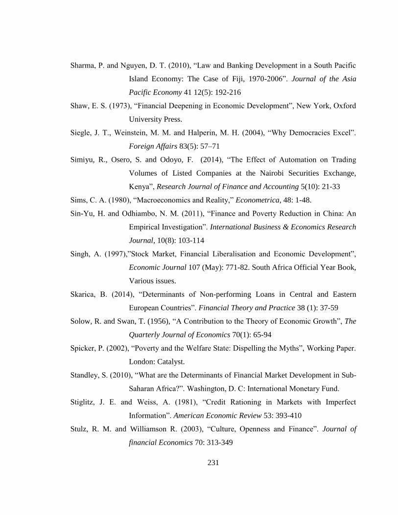
231
Sharma, P. and Nguyen, D. T. (2010), ―Law and Banking Development in a South Pacific
Island Economy: The Case of Fiji, 1970-2006‖. Journal of the Asia
Pacific Economy 41 12(5): 192-216
Shaw, E. S. (1973), ―Financial Deepening in Economic Development‖, New York, Oxford
University Press.
Siegle, J. T., Weinstein, M. M. and Halperin, M. H. (2004), ―Why Democracies Excel‖.
Foreign Affairs 83(5): 57–71
Simiyu, R., Osero, S. and Odoyo, F. (2014), ―The Effect of Automation on Trading
Volumes of Listed Companies at the Nairobi Securities Exchange,
Kenya‖, Research Journal of Finance and Accounting 5(10): 21-33
Sims, C. A. (1980), ―Macroeconomics and Reality,‖ Econometrica, 48: 1-48.
Sin-Yu, H. and Odhiambo, N. M. (2011), ―Finance and Poverty Reduction in China: An
Empirical Investigation‖. International Business & Economics Research
Journal, 10(8): 103-114
Singh, A. (1997),‖Stock Market, Financial Liberalisation and Economic Development‖,
Economic Journal 107 (May): 771-82. South Africa Official Year Book,
Various issues.
Skarica, B. (2014), ―Determinants of Non-performing Loans in Central and Eastern
European Countries‖. Financial Theory and Practice 38 (1): 37-59
Solow, R. and Swan, T. (1956), ―A Contribution to the Theory of Economic Growth‖, The
Quarterly Journal of Economics 70(1): 65-94
Spicker, P. (2002), ―Poverty and the Welfare State: Dispelling the Myths‖, Working Paper.
London: Catalyst.
Standley, S. (2010), ―What are the Determinants of Financial Market Development in Sub-
Saharan Africa?‖. Washington, D. C: International Monetary Fund.
Stiglitz, J. E. and Weiss, A. (1981), ―Credit Rationing in Markets with Imperfect
Information‖. American Economic Review 53: 393-410
Stulz, R. M. and Williamson R. (2003), ―Culture, Openness and Finance‖. Journal of
financial Economics 70: 313-349
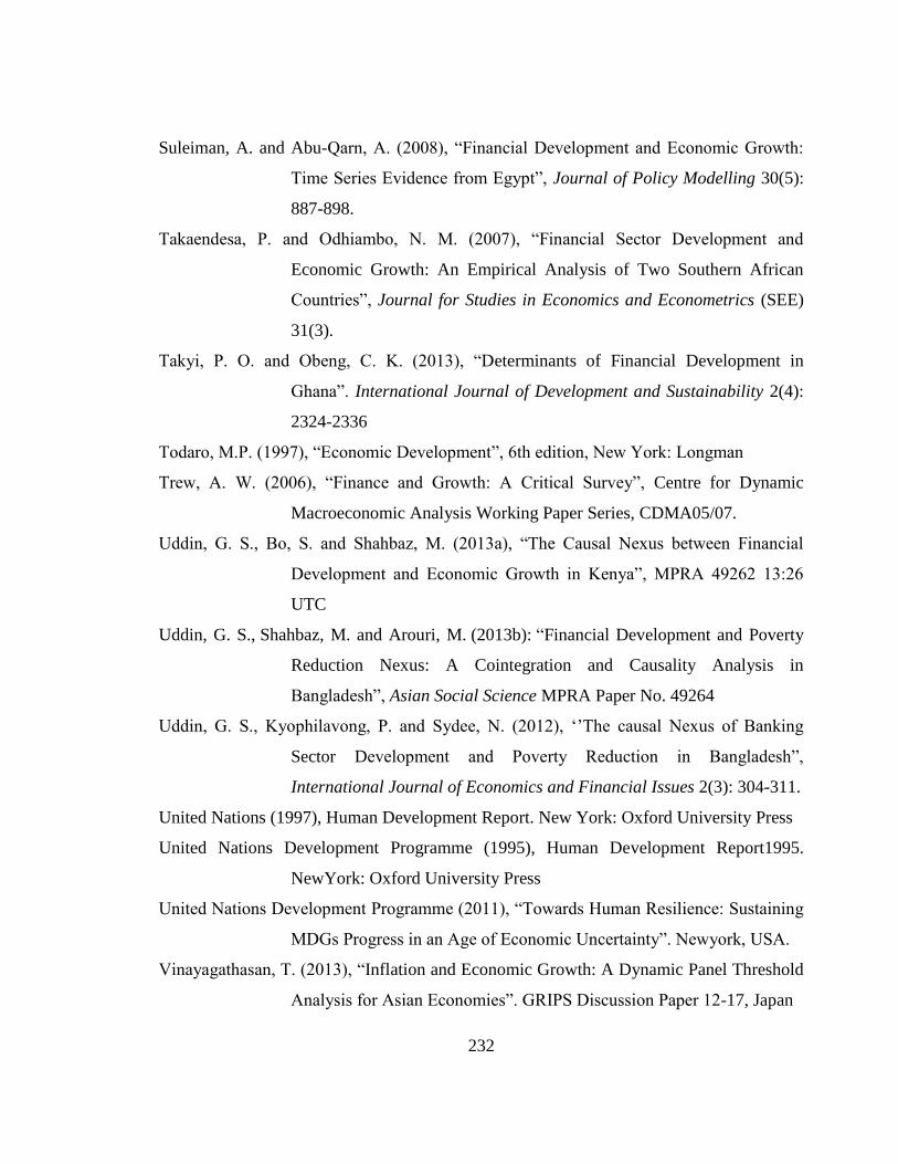
232
Suleiman, A. and Abu-Qarn, A. (2008), ―Financial Development and Economic Growth:
Time Series Evidence from Egypt‖, Journal of Policy Modelling 30(5):
887-898.
Takaendesa, P. and Odhiambo, N. M. (2007), ―Financial Sector Development and
Economic Growth: An Empirical Analysis of Two Southern African
Countries‖, Journal for Studies in Economics and Econometrics (SEE)
31(3).
Takyi, P. O. and Obeng, C. K. (2013), ―Determinants of Financial Development in
Ghana‖. International Journal of Development and Sustainability 2(4):
2324-2336
Todaro, M.P. (1997), ―Economic Development‖, 6th edition, New York: Longman
Trew, A. W. (2006), ―Finance and Growth: A Critical Survey‖, Centre for Dynamic
Macroeconomic Analysis Working Paper Series, CDMA05/07.
Uddin, G. S., Bo, S. and Shahbaz, M. (2013a), ―The Causal Nexus between Financial
Development and Economic Growth in Kenya‖, MPRA 49262 13:26
UTC
Uddin, G. S., Shahbaz, M. and Arouri, M. (2013b): ―Financial Development and Poverty
Reduction Nexus: A Cointegration and Causality Analysis in
Bangladesh‖, Asian Social Science MPRA Paper No. 49264
Uddin, G. S., Kyophilavong, P. and Sydee, N. (2012), ‗‘The causal Nexus of Banking
Sector Development and Poverty Reduction in Bangladesh‖,
International Journal of Economics and Financial Issues 2(3): 304-311.
United Nations (1997), Human Development Report. New York: Oxford University Press
United Nations Development Programme (1995), Human Development Report1995.
NewYork: Oxford University Press
United Nations Development Programme (2011), ―Towards Human Resilience: Sustaining
MDGs Progress in an Age of Economic Uncertainty‖. Newyork, USA.
Vinayagathasan, T. (2013), ―Inflation and Economic Growth: A Dynamic Panel Threshold
Analysis for Asian Economies‖. GRIPS Discussion Paper 12-17, Japan

233
Voghouei, H., Azali, M. and Jamali, M. A. (2011a), ―A Survey of the Determinants of
Financial Development‖. Asian-Pacific Economic Literature 25(2): 1–
20
Voghouei, H., Azali, M. and Law, S. H. (2011b), ―Does the Political Institutions Matter for
Financial Development?‖ Economic Papers 30(1): 77–98
Voghouei, H., Azali, M. and Law, S. H. (2010), ―The Effect of Dynamic Legal Tradition
on Financial Development: Panel Data Evidence‖. European Journal of
Law and Economics, doi: 10.1007/s10657- 010-9191-x
Waqabaca, C. (2004), ―Financial Development and Economic Growth in Fiji‖, Working
Paper 2004/03 (December), Economics Department, Reserve Bank of
Fiji.
Were, M. and Wambua, J. (2013), ―Assessing the Determinants of Interest Rate Spread of
Commercial Banks in Kenya: An Empirical Investigation‖, Kenya
Bankers Association Working Paper Series No. WPS/01/13.
Were, M. and Wambua, J. (2014), ―What Factors Drive Interest Rate Spread of
Commercial Banks? Empirical Evidence from Kenya‖, Review of
development Finance 4(2): 73-82
Wolde-Rufael, Y. (2009), ―Re-examining the financial development and economic growth
nexus in Kenya‖, Economic Modelling 26: 1140 — 1146.
Wood, A. (1993), ―Financial Development and Economic Growth in Barbados, Causal
Evidence‖ Savings and Development 17(4): 379-389.
Woolard, I. and Leibbrandt, M. (1999), ―Measuring Poverty in South Africa‖, DPRU
Working Papers No. 99/3, Development Policy Research Unit,
University of Cape Town
World Bank (2016), Global Economic Prospect: Divergences and Risks. Washington D.C:
World Bank
World Bank (2014a), Kenya Economic Update: Anchoring High Growth: Can
Manufacturing Contribute More? No. 11, December 2014. Washington
D.C: World Bank
234
World Bank (2014b), World Development Indicators. Washington D.C: World Bank.
World Bank (2013a), Kenya Economic Update: Time to shift gears: Accelerating growth
and poverty reduction in the New Kenya. No. 8, June 2013
World Bank (2013b), Developing Kenya‘s Mortgage Market. Washington DC, WorldBank
World Bank (2013c), ―Global Financial Development‖, Washington DC, World Bank
World Bank (2006), ―Measuring Banking Sector developments‖, Washington DC: World
Bank
World Bank (2002), ―Capital Market Integration in the East African Community‖,
Washington, DC, World Bank. No. 14.
World Bank (1990), World Development Report 1990: Poverty. Newyork: Oxford
University Press.
Xu, Z. (2000), ―Financial Development, Investment and Economic Growth‖, Economic
Inquiry 331 - 344.
Yang, B. (2011), ―Does Democracy Foster Financial Development? An Empirical
Analysis‖. Economics Letters 112(3): 262- 265.
Yartey, C. A. (2007), ―Well-developed Financial Intermediary Sector Promotes Stock
Development: Evidence from Africa‖, Journal of Emerging Market
Finance 6(3): 269–8
Yu, H. and Gan, P. T. (2010), ―The Determinants of Banking Sector Development:
Malaysian Experience‖. International Research Journal of Finance and
Economics 35: 29-35.
Zivot, E. and Andrews, W. K. (1992), ―Further Evidence on the Great Crash, the Oil Price
Shock and the Unit Root Hypothesis‖, Journal of Business and
Economics Statistics 10: 251-270
Zoli, E. (2007), ―Financial Development in Emerging Europe: The Unfinished Agenda‖.
IMF Working Paper No. WP/07/245
235
APPENDIX
Figure A.1: Relationship between M-Pesa Agents and Credit to Private Sector
Figure A.2: Relationship between M-Pesa Agents and Non-Performing Loans (NPL)
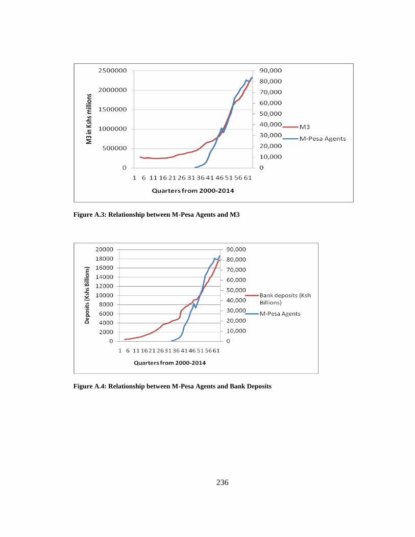
236
Figure A.3: Relationship between M-Pesa Agents and M3
Figure A.4: Relationship between M-Pesa Agents and Bank Deposits

237
14.7
14.8
14.9
15.0
15.1
15.2
15.3
15.4
00 01 02 03 04 05 06 07 08 09 10 11 12 13 14
GDP
Figure A.5: Trend in Real GDP
12.0
12.4
12.8
13.2
13.6
14.0
14.4
14.8
01 02 03 04 05 06 07 08 09 10 11 12 13 14 15
CPS
Figure A.6: Trend in Credit to Private Sector
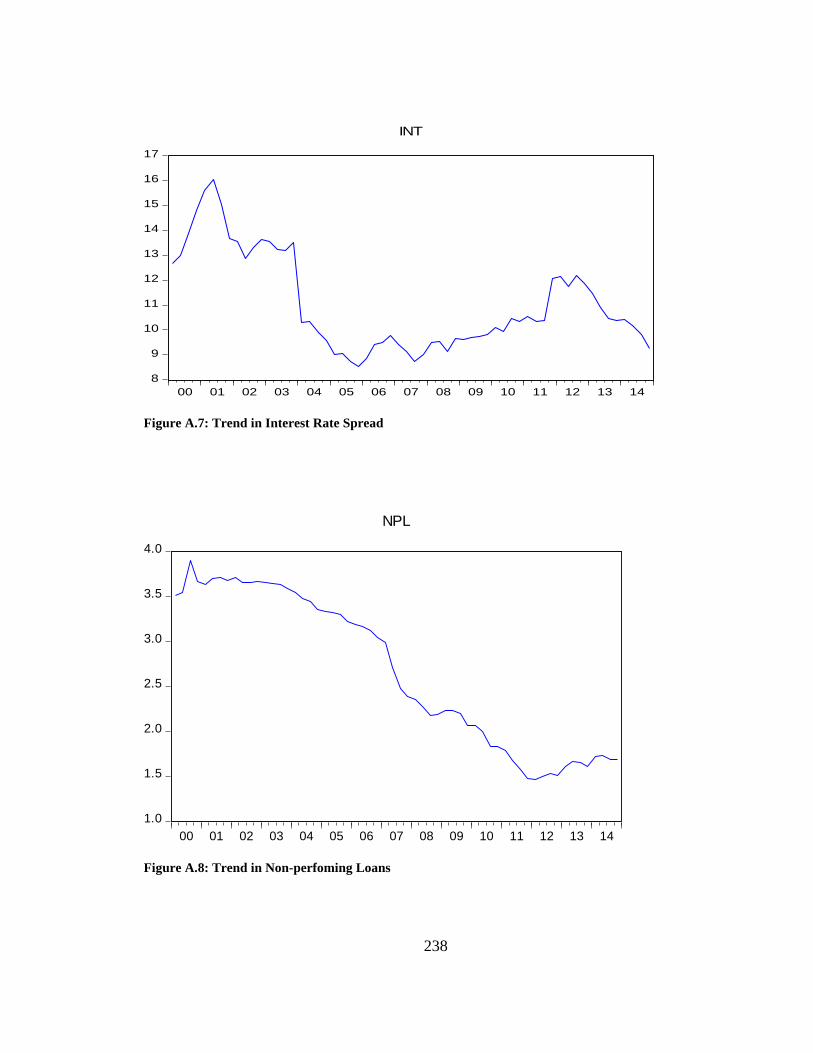
238
8
9
10
11
12
13
14
15
16
17
00 01 02 03 04 05 06 07 08 09 10 11 12 13 14
INT
Figure A.7: Trend in Interest Rate Spread
1.0
1.5
2.0
2.5
3.0
3.5
4.0
00 01 02 03 04 05 06 07 08 09 10 11 12 13 14
NPL
Figure A.8: Trend in Non-perfoming Loans

239
11.2
11.6
12.0
12.4
12.8
13.2
13.6
14.0
14.4
14.8
00 01 02 03 04 05 06 07 08 09 10 11 12 13 14
MKT
Figure A.9: Trend in Market Capitalization
8
9
10
11
12
13
14
15
16
17
00 01 02 03 04 05 06 07 08 09 10 11 12 13 14
INT
Figure A.10: Trend in Interest Rate Spread

240
3.70
3.75
3.80
3.85
3.90
3.95
4.00
4.05
4.10
00 01 02 03 04 05 06 07 08 09 10 11 12 13 14
OPEN
Figure A.11: Trend in Trade Openness
9.65
9.70
9.75
9.80
9.85
9.90
9.95
00 01 02 03 04 05 06 07 08 09 10 11 12 13 14
GDPPC
Figure A.12: Trend in GDP Per Capita

241
3.80
3.82
3.84
3.86
3.88
3.90
3.92
3.94
00 01 02 03 04 05 06 07 08 09 10 11 12 13 14
HCR
Figure A.13: Trend in Head Count Ratio
9.40
9.44
9.48
9.52
9.56
9.60
9.64
9.68
9.72
00 01 02 03 04 05 06 07 08 09 10 11 12 13 14
PCC
Figure A.14: Trend in Per Capita Consumption

242
2.8
3.2
3.6
4.0
4.4
4.8
5.2
5.6
01 02 03 04 05 06 07 08 09 10 11 12 13 14 15
DA
Figure A.15: Trend in Democratic Accountability
1.6
1.8
2.0
2.2
2.4
2.6
2.8
3.0
01 02 03 04 05 06 07 08 09 10 11 12 13 14 15
INST
Figure A.16: Trend in Institutional Quality

243
9.0
9.5
10.0
10.5
11.0
11.5
12.0
01 02 03 04 05 06 07 08 09 10 11 12 13 14 15
REM
Figure A.17: Trend in Remittances
9
10
11
12
13
14
15
16
17
18
01 02 03 04 05 06 07 08 09 10 11 12 13 14 15
TECH
Figure A.18: Trend in Technology

244
Table A.1: Optimal Lag Length Results
Variable Lags FPE AIC HQIC SBIC
LNCredit to Private Sector 3 0.0028* 3.0280* 2.9716* 2.8821*
LNMarket Capitalization 1 0.0227* 0.9473* 0.9191* 0.8743*
LNNon-performing Loans 3 0.0049* 2.4678* 2.4257* 2.3592*
LNGDP per Capita 2 0.000049* -7.09293* -7.04977* -6.98035*
LNReal GDP 1 0.0029* 3.0072* 2.9792* 2.9349*
LNInflation 4 0.1234* 0.7447* 0.8149* 0.9256*
LNInterest Rate Spread 1 0.0029* 3.0072* 2.9792* 2.9349*
LNTrade Openness 3 0.0022* 3.2786* 3.2222* Significant at lag 1
LNInstitutional Quality 1 0.0040* -2.6837* -2.6556* -2.6114*
LNDemocratic Quality 1 0.1959* -1.0945* -1.0524* -0.9859*
LNRemittances 3 0.0061* -2.2611* -2.2330* -2.1887*
LNTechnology 4 0.0057* -2.3281* -2.2579* -2.1472*
LNPer Capita Consumption 2 0.000049* -7.09293* -7.04977* -6.98035*
LNHead Count Ratio 1 0.000612* -4.56098* -4.53221* -4.48593*
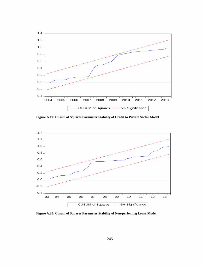
245
-0.4
-0.2
0.0
0.2
0.4
0.6
0.8
1.0
1.2
1.4
2004 2005 2006 2007 2008 2009 2010 2011 2012 2013
CUSUM of Squares 5% Significance
Figure A.19: Cusum of Squares Parameter Stability of Credit to Private Sector Model
-0.4
-0.2
0.0
0.2
0.4
0.6
0.8
1.0
1.2
1.4
03 04 05 06 07 08 09 10 11 12 13
CUSUM of Squares 5% Significance
Figure A.20: Cusum of Squares Parameter Stability of Non-perfoming Loans Model

246
-0.4
-0.2
0.0
0.2
0.4
0.6
0.8
1.0
1.2
1.4
03 04 05 06 07 08 09 10 11 12 13
CUSUM of Squares 5% Significance
Figure A.21: Cusum of Squares Parameter Stability of Market Capitalization Model
Table A.2: Short-run Regression Results of the Market Capitalization Model
Dependent Variable: LNMarket Capitalization
Variable Co-efficients
LNTrade Openness -0.129
(0.703)
LNInstitutional Quality 0.473**
(0.010)
LNGDP Per Capita 2.848**
(0.002)
LNInflation 0.056
(0.213)
LNDemocratic Accountability 0.569**
(0.000)
LNRemittances -0.181
(0.179)
LNTechnology 0.151**
(0.002)
** Significant at 5 Percent Significance Level
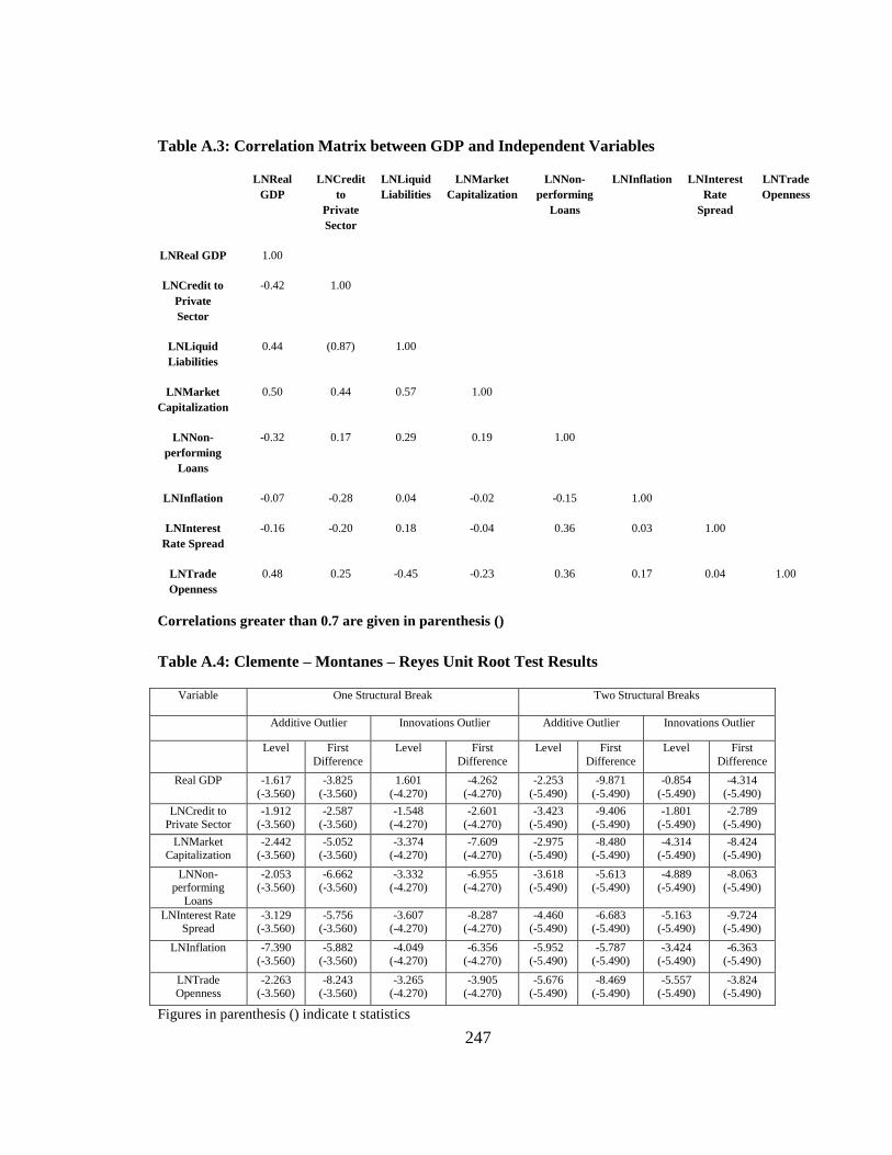
247
Table A.3: Correlation Matrix between GDP and Independent Variables
Correlations greater than 0.7 are given in parenthesis ()
Table A.4: Clemente – Montanes – Reyes Unit Root Test Results
Variable One Structural Break Two Structural Breaks
Additive Outlier Innovations Outlier Additive Outlier Innovations Outlier
Level First
Difference
Level First
Difference
Level First
Difference
Level First
Difference
Real GDP -1.617
(-3.560)
-3.825
(-3.560)
1.601
(-4.270)
-4.262
(-4.270)
-2.253
(-5.490)
-9.871
(-5.490)
-0.854
(-5.490)
-4.314
(-5.490)
LNCredit to Private Sector
-1.912 (-3.560)
-2.587 (-3.560)
-1.548 (-4.270)
-2.601 (-4.270)
-3.423 (-5.490)
-9.406 (-5.490)
-1.801 (-5.490)
-2.789 (-5.490)
LNMarket Capitalization
-2.442 (-3.560)
-5.052 (-3.560)
-3.374 (-4.270)
-7.609 (-4.270)
-2.975 (-5.490)
-8.480 (-5.490)
-4.314 (-5.490)
-8.424 (-5.490)
LNNon-performing
Loans
-2.053 (-3.560)
-6.662 (-3.560)
-3.332 (-4.270)
-6.955 (-4.270)
-3.618 (-5.490)
-5.613 (-5.490)
-4.889 (-5.490)
-8.063 (-5.490)
LNInterest Rate Spread
-3.129 (-3.560)
-5.756 (-3.560)
-3.607 (-4.270)
-8.287 (-4.270)
-4.460 (-5.490)
-6.683 (-5.490)
-5.163 (-5.490)
-9.724 (-5.490)
LNInflation -7.390 (-3.560)
-5.882 (-3.560)
-4.049 (-4.270)
-6.356 (-4.270)
-5.952 (-5.490)
-5.787 (-5.490)
-3.424 (-5.490)
-6.363 (-5.490)
LNTrade Openness
-2.263 (-3.560)
-8.243 (-3.560)
-3.265 (-4.270)
-3.905 (-4.270)
-5.676 (-5.490)
-8.469 (-5.490)
-5.557 (-5.490)
-3.824 (-5.490)
Figures in parenthesis () indicate t statistics
LNReal
GDP
LNCredit
to
Private
Sector
LNLiquid
Liabilities
LNMarket
Capitalization
LNNon-
performing
Loans
LNInflation LNInterest
Rate
Spread
LNTrade
Openness
LNReal GDP 1.00
LNCredit to
Private
Sector
-0.42 1.00
LNLiquid
Liabilities
0.44 (0.87) 1.00
LNMarket
Capitalization
0.50 0.44 0.57 1.00
LNNon-
performing
Loans
-0.32 0.17 0.29 0.19 1.00
LNInflation -0.07 -0.28 0.04 -0.02 -0.15 1.00
LNInterest
Rate Spread
-0.16 -0.20 0.18 -0.04 0.36 0.03 1.00
LNTrade
Openness
0.48 0.25 -0.45 -0.23 0.36 0.17 0.04 1.00
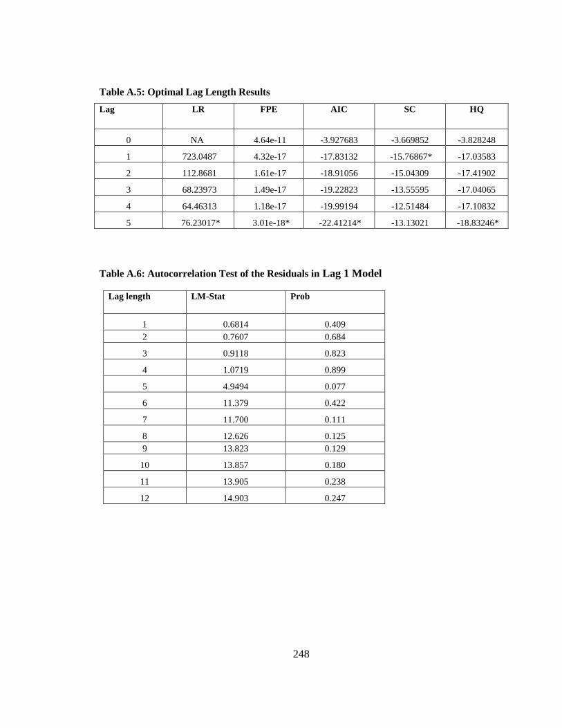
248
Table A.5: Optimal Lag Length Results
Lag LR FPE AIC SC HQ
0 NA 4.64e-11 -3.927683 -3.669852 -3.828248
1 723.0487 4.32e-17 -17.83132 -15.76867* -17.03583
2 112.8681 1.61e-17 -18.91056 -15.04309 -17.41902
3 68.23973 1.49e-17 -19.22823 -13.55595 -17.04065
4 64.46313 1.18e-17 -19.99194 -12.51484 -17.10832
5 76.23017* 3.01e-18* -22.41214* -13.13021 -18.83246*
Table A.6: Autocorrelation Test of the Residuals in Lag 1 Model
Lag length LM-Stat Prob
1 0.6814 0.409
2 0.7607 0.684
3 0.9118 0.823
4 1.0719 0.899
5 4.9494 0.077
6 11.379 0.422
7 11.700 0.111
8 12.626 0.125
9 13.823 0.129
10 13.857 0.180
11 13.905 0.238
12 14.903 0.247
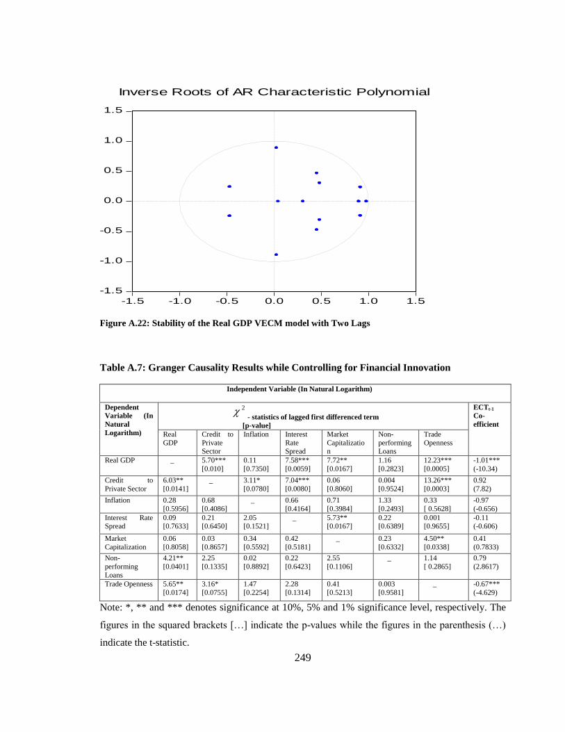
249
-1.5
-1.0
-0.5
0.0
0.5
1.0
1.5
-1.5 -1.0 -0.5 0.0 0.5 1.0 1.5
Inverse Roots of AR Characteristic Polynomial
Figure A.22: Stability of the Real GDP VECM model with Two Lags
Table A.7: Granger Causality Results while Controlling for Financial Innovation
Independent Variable (In Natural Logarithm)
Dependent
Variable (In
Natural
Logarithm)
2- statistics of lagged first differenced term
[p-value]
ECTt-1
Co-
efficient
Real
GDP
Credit to
Private Sector
Inflation Interest
Rate Spread
Market
Capitalization
Non-
performing Loans
Trade
Openness
Real GDP _ 5.70***
[0.010]
0.11
[0.7350]
7.58***
[0.0059]
7.72**
[0.0167]
1.16
[0.2823]
12.23***
[0.0005]
-1.01***
(-10.34)
Credit to
Private Sector
6.03**
[0.0141]
_ 3.11*
[0.0780]
7.04***
[0.0080]
0.06
[0.8060]
0.004
[0.9524]
13.26***
[0.0003]
0.92
(7.82)
Inflation 0.28
[0.5956]
0.68
[0.4086]
_ 0.66
[0.4164]
0.71
[0.3984]
1.33
[0.2493]
0.33
[ 0.5628]
-0.97
(-0.656)
Interest Rate Spread
0.09 [0.7633]
0.21 [0.6450]
2.05 [0.1521]
_ 5.73** [0.0167]
0.22 [0.6389]
0.001 [0.9655]
-0.11 (-0.606)
Market
Capitalization
0.06
[0.8058]
0.03
[0.8657]
0.34
[0.5592]
0.42
[0.5181]
_ 0.23
[0.6332]
4.50**
[0.0338]
0.41
(0.7833)
Non-
performing
Loans
4.21**
[0.0401]
2.25
[0.1335]
0.02
[0.8892]
0.22
[0.6423]
2.55
[0.1106]
_ 1.14
[ 0.2865]
0.79
(2.8617)
Trade Openness 5.65**
[0.0174]
3.16*
[0.0755]
1.47
[0.2254]
2.28
[0.1314]
0.41
[0.5213]
0.003
[0.9581]
_ -0.67***
(-4.629)
Note: *, ** and *** denotes significance at 10%, 5% and 1% significance level, respectively. The
figures in the squared brackets […] indicate the p-values while the figures in the parenthesis (…)
indicate the t-statistic.
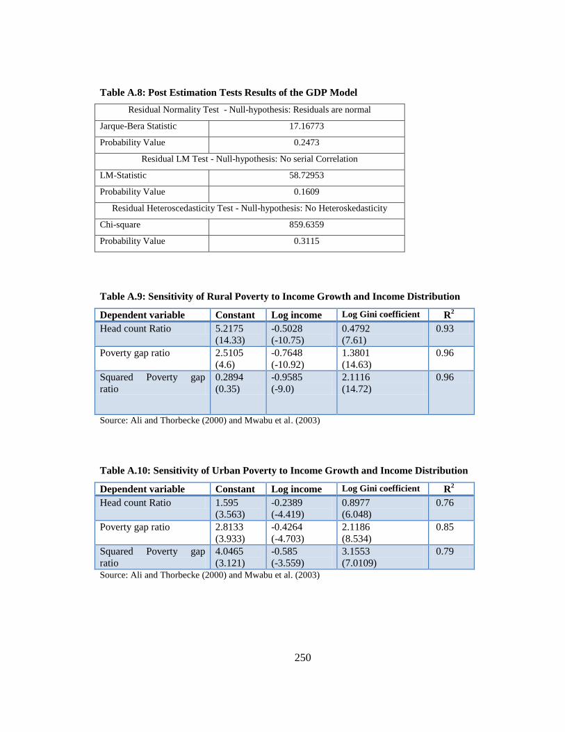
250
Table A.8: Post Estimation Tests Results of the GDP Model
Residual Normality Test - Null-hypothesis: Residuals are normal
Jarque-Bera Statistic 17.16773
Probability Value 0.2473
Residual LM Test - Null-hypothesis: No serial Correlation
LM-Statistic 58.72953
Probability Value 0.1609
Residual Heteroscedasticity Test - Null-hypothesis: No Heteroskedasticity
Chi-square 859.6359
Probability Value 0.3115
Table A.9: Sensitivity of Rural Poverty to Income Growth and Income Distribution
Dependent variable Constant Log income Log Gini coefficient R2
Head count Ratio 5.2175
(14.33)
-0.5028
(-10.75)
0.4792
(7.61)
0.93
Poverty gap ratio 2.5105
(4.6)
-0.7648
(-10.92)
1.3801
(14.63)
0.96
Squared Poverty gap
ratio
0.2894
(0.35)
-0.9585
(-9.0)
2.1116
(14.72)
0.96
Source: Ali and Thorbecke (2000) and Mwabu et al. (2003)
Table A.10: Sensitivity of Urban Poverty to Income Growth and Income Distribution
Dependent variable Constant Log income Log Gini coefficient R2
Head count Ratio 1.595
(3.563)
-0.2389
(-4.419)
0.8977
(6.048)
0.76
Poverty gap ratio 2.8133
(3.933)
-0.4264
(-4.703)
2.1186
(8.534)
0.85
Squared Poverty gap
ratio
4.0465
(3.121)
-0.585
(-3.559)
3.1553
(7.0109)
0.79
Source: Ali and Thorbecke (2000) and Mwabu et al. (2003)

251
Table A.11: Sensitivity of National Poverty to Income Growth and Income Distribution
Dependent variable Constant Log income Log Gini coefficient
Head count Ratio 3.3685
(8.9464)
-0.37085
(-7.584)
0.68845
(6.829)
Poverty gap ratio 2.6619
(4.267)
-0.5956
(-7.8115)
1.74935
(11.582)
Squared Poverty gap ratio 2.16795
(1.7355)
-0.77175
(6.279)
2.63345
(10.865) Author‘s own calculations based on Table A.11 and A.12
Table A.12: Correlation Matrix with Per Capita Consumption
LNPer Capita
Consumption
LNGDP
Per
Capita
LNCredit
to
Private
Sector
LNNon-
Performing
Loans
LNInflation LNInterest
Rate
Spread
LNTrade
Openness
LNPer Capita
Consumption
1.00
LNGDP Per
Capita
0.12 1.00
LNCredit to
Private Sector
-0.12 -0.42 1.00
LNNon-
Performing Loans
0.06 -0.22 0.22 1.00
LNInflation -0.22 -0.07 -0.18 -0.04 1.00
LNInterest Rate
Spread
-0.24 -0.04 -0.05 0.41 0.06 1.00
LNTrade
Openness
0.10 0.38 0.07 0.04 0.11 0.06 1.00

252
Table A.13: Correlation Matrix with Head Count Ratio
Table A.14: Optimal Lag Length of the Model with Per Capita Consumption
Lag LR FPE AIC SC HQ
0 NA 4.04e-13 -8.6719 -8.4093 -8.5712
1 661.8832 7.93e-19 -21.830 -19.7288 -21.0245
2 139.1657 1.34e-19 -23.707 -19.7668* -22.1962
3 63.24045 1.42e-19 -23.9301 -18.1515 -21.7147
4 101.7933* 2.05e-20* -26.4713* -18.8539 -23.5510*
* indicates lag order selected by the criterion at 5% significance level
LNHead
Count Ratio
LNGDP
Per
Capita
LNCredit
to Private
Sector
LNNon-
Performing
Loans
LNInflatio
n
LNInterest
Rate Spread
LNTrade
Openness
LNHead Count
Ratio
1.00
LNGDP Per
Capita
-0.08 1.00
LNCredit to
Private Sector
-0.09 -0.42 1.00
LNNon-
Performing
Loans
0.09 -0.22 0.26 1.00
LNInflation 0.28 -0.08 -0.18 -0.02 1.00
LNInterest Rate
Spread
0.16 -0.04 -0.08 0.40 0.06 1.00
LNTrade
Openness
-0.10 0.48 0.06 0.02 0.11 0.13 1.00
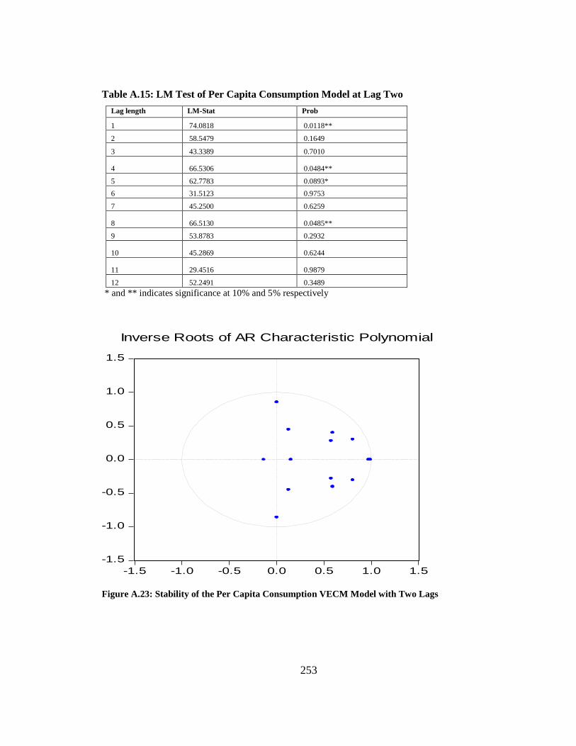
253
Table A.15: LM Test of Per Capita Consumption Model at Lag Two
Lag length LM-Stat Prob
1 74.0818 0.0118**
2 58.5479 0.1649
3 43.3389 0.7010
4 66.5306 0.0484**
5 62.7783 0.0893*
6 31.5123 0.9753
7 45.2500 0.6259
8 66.5130 0.0485**
9 53.8783 0.2932
10 45.2869 0.6244
11 29.4516 0.9879
12 52.2491 0.3489
* and ** indicates significance at 10% and 5% respectively
-1.5
-1.0
-0.5
0.0
0.5
1.0
1.5
-1.5 -1.0 -0.5 0.0 0.5 1.0 1.5
Inverse Roots of AR Characteristic Polynomial
Figure A.23: Stability of the Per Capita Consumption VECM Model with Two Lags

254
Table A.16: Optimal Lag Length of the Head Count Ratio Model
Lag LR FPE AIC SC HQ
0 NA 5.99e-13 -8.278420 -8.013267 -8.177097
1 580.7014 5.69e-18 -19.86153 -16.94334 -19.05095
2 107.3037 2.19e-18 -20.92062 -17.74031* -19.40079
3 68.51219* 1.90e-18 -21.36155 -15.52819 -19.13245
4 65.87517 1.25e-18* -22.43430* -14.74488 -19.49595*
Table A.17: LM Test of Head Count Ratio Model at Various Lags
Lag length Model at lag 2 Model at lag 3 Model at lag 4
LM-Stat Prob LM-Stat Prob LM-Stat Prob
1 61.40685 0.1099 106.7643 0.0000** 42.59559 0.7288
2 48.31430 0.5008 56.32301 0.2199 39.13595 0.8423
3 55.19192 0.2522 79.46646 0.0038** 58.22306 0.1723
4 55.36662 0.2470 89.30649 0.0004** 64.31918 0.0699*
5 60.63419 0.1231 61.57016 0.1073 41.12980 0.7805
6 37.87295 0.8757 81.30631 0.0025** 45.69672 0.6078
7 53.19495 0.3159 65.20342 0.0605* 52.24921 0.3489
8 58.79231 0.1595 80.41507 0.0031** 75.13502 0.0096**
9 48.28450 0.5021 58.25858 0.1714 65.32527 0.0593*
10 54.39581 0.2766 67.76925 0.0390** 47.06637 0.5518
11 36.12776 0.9141 57.29386 0.1946 49.45397 0.4550
12 53.00519 0.3224 58.54731 0.1649 47.78774 0.5223
* and ** indicates significance at 10% and 5% respectively
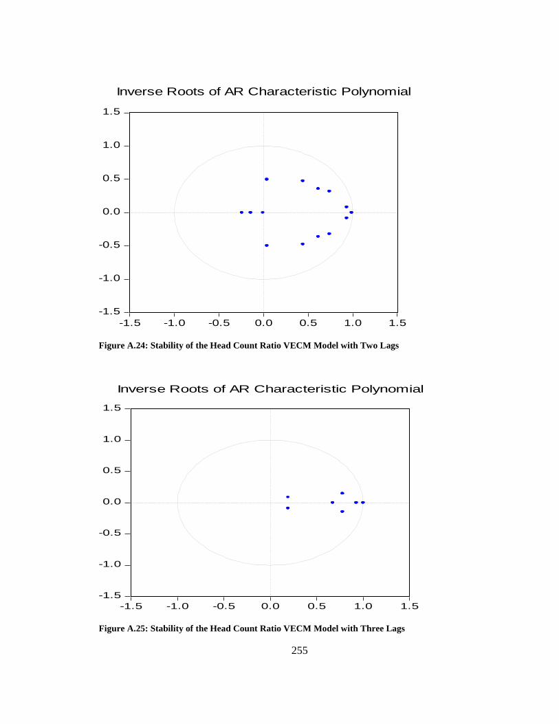
255
-1.5
-1.0
-0.5
0.0
0.5
1.0
1.5
-1.5 -1.0 -0.5 0.0 0.5 1.0 1.5
Inverse Roots of AR Characteristic Polynomial
Figure A.24: Stability of the Head Count Ratio VECM Model with Two Lags
-1.5
-1.0
-0.5
0.0
0.5
1.0
1.5
-1.5 -1.0 -0.5 0.0 0.5 1.0 1.5
Inverse Roots of AR Characteristic Polynomial
Figure A.25: Stability of the Head Count Ratio VECM Model with Three Lags
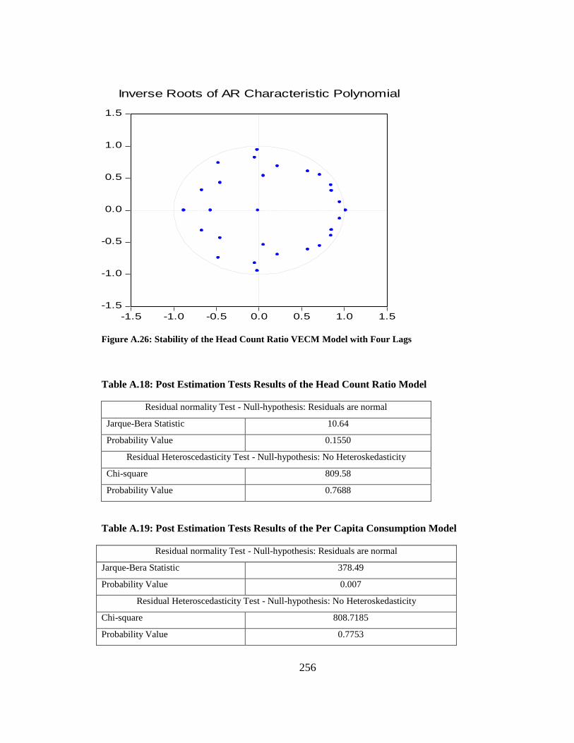
256
-1.5
-1.0
-0.5
0.0
0.5
1.0
1.5
-1.5 -1.0 -0.5 0.0 0.5 1.0 1.5
Inverse Roots of AR Characteristic Polynomial
Figure A.26: Stability of the Head Count Ratio VECM Model with Four Lags
Table A.18: Post Estimation Tests Results of the Head Count Ratio Model
Residual normality Test - Null-hypothesis: Residuals are normal
Jarque-Bera Statistic 10.64
Probability Value 0.1550
Residual Heteroscedasticity Test - Null-hypothesis: No Heteroskedasticity
Chi-square 809.58
Probability Value 0.7688
Table A.19: Post Estimation Tests Results of the Per Capita Consumption Model
Residual normality Test - Null-hypothesis: Residuals are normal
Jarque-Bera Statistic 378.49
Probability Value 0.007
Residual Heteroscedasticity Test - Null-hypothesis: No Heteroskedasticity
Chi-square 808.7185
Probability Value 0.7753

257
Table A.20: Predicted Quarterly Head Count Ratio for the Period 2001 – 2014
Period Predicted Poverty
(Head Count Ratio)
Period Predicted Poverty (Head
Count Ratio)
2001q1 50.1 2008q1 48.8
2001q2 48.6 2008q2 48.8
2001q3 48.5 2008q3 48.7
2001q4 49.7 2008q4 48.5
2002q1 49.3 2009q1 48.3
2002q2 50.8 2009q2 48.3
2002q3 50.8 2009q3 48.1
2002q4 50.7 2009q4 48.1
2003q1 50.8 2010q1 47.7
2003q2 49.7 2010q2 47.1
2003q3 48.4 2010q3 46.9
2003q4 48.9 2010q4 46.9
2004q1 48.3 2011q1 47.3
2004q2 49.0 2011q2 47.6
2004q3 49.1 2011q3 47.9
2004q4 48.9 2011q4 48.4
2005q1 46.8 2012q1 48.4
2005q2 45.8 2012q2 48.6
2005q3 45.5 2012q3 48.5
2005q4 46.5 2012q4 48.4
2006q1 46.4 2013q1 47.6
2006q2 46.3 2013q2 47.2
2006q3 45.5 2013q3 47.3
2006q4 46.8 2013q4 48.8
2007q1 45.5 2014q1 47.7
2007q2 45.1 2014q2 47.2
2007q3 45.8 2014q3 47.5
2007q4 45.8 2014q4 47.4