Finance and Economics Discussion Series Divisions of Research & Statistics and Monetary Affairs

Federal Reserve Board, Washington, D.C.

Housing and the Monetary Transmission Mechanism

Frederic S. Mishkin

2007-40

NOTE: Staff working papers in the Finance and Economics Discussion Series (FEDS) are preliminary materials circulated to stimulate discussion and critical comment. The analysis and conclusions set forth are those of the authors and do not indicate concurrence by other members of the research staff or the Board of Governors. References in publications to the Finance and Economics Discussion Series (other than acknowledgement) should be cleared with the author(s) to protect the tentative character of these papers.

Housing and the Monetary Transmission Mechanism

Frederic S. Mishkin

Member

Board of Governors of the Federal Reserve System

August 2007

Prepared for Federal Reserve Bank of Kansas City’s 2007 Jackson Hole Symposium, Jackson Hole, Wyoming. The views expressed here are my own and are not necessarily those of the Board of Governors or the Federal Reserve System. For their helpful comments and other contributions, I would like to thank Sally Davies, Brian Doyle, Wendy Edelberg, Rochelle Edge, Linda Kole, Andreas Lehnert, Michael Palumbo, Richard Peach, David Reifschneider, Raven Saks, and Robert Tetlow.

1

The housing market seems to be on everybody’s mind these days, and for good

reason: Developments in the housing market have a major effect on economic activity.

For example, as single-family housing starts in the United States dropped from their peak

of 1.84 million units in January 2006 to the current level of 1.15 million units, the

accompanying contraction in residential investment is estimated to have lowered the

growth of gross domestic product over the last four quarters by a full percentage point.

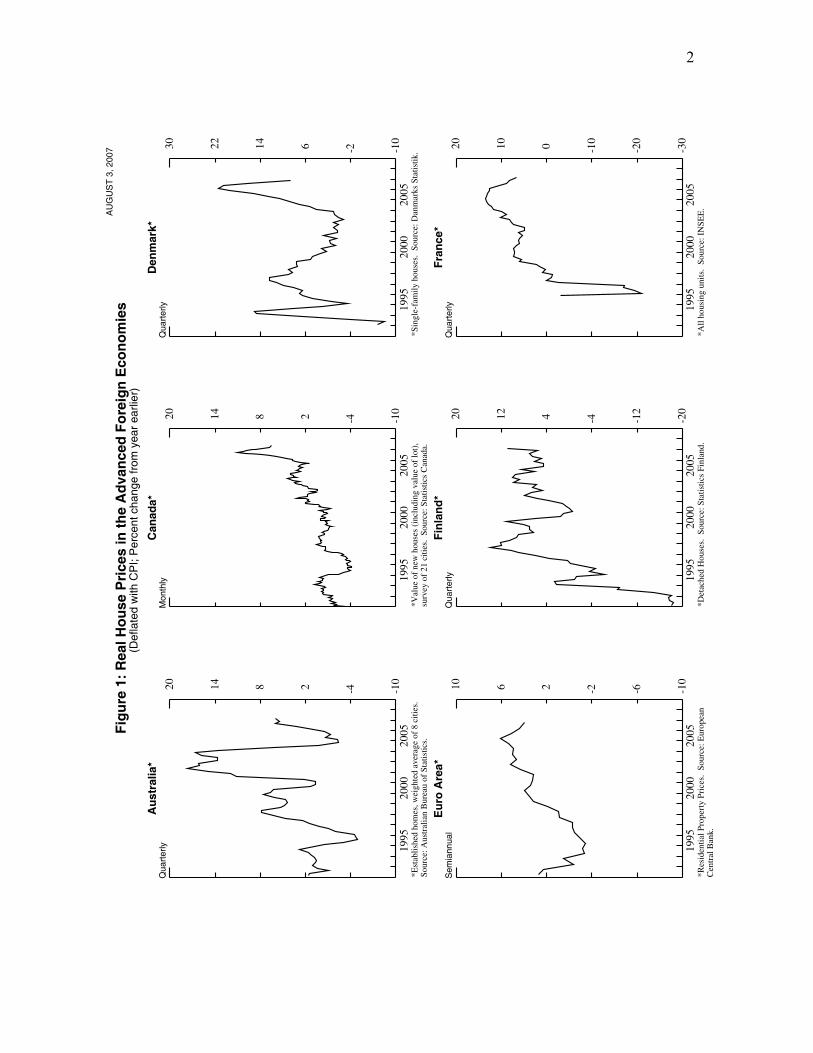
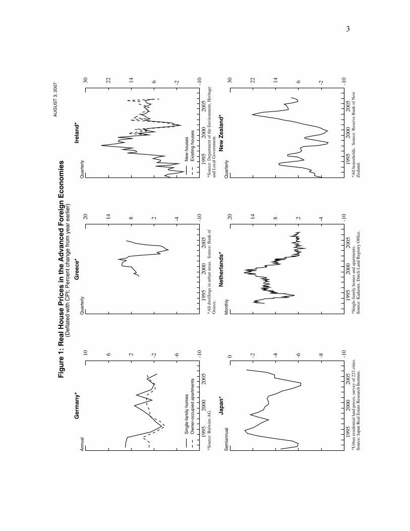
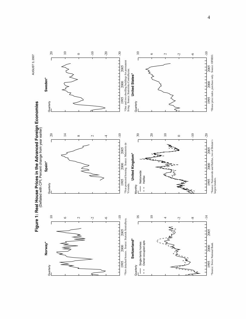
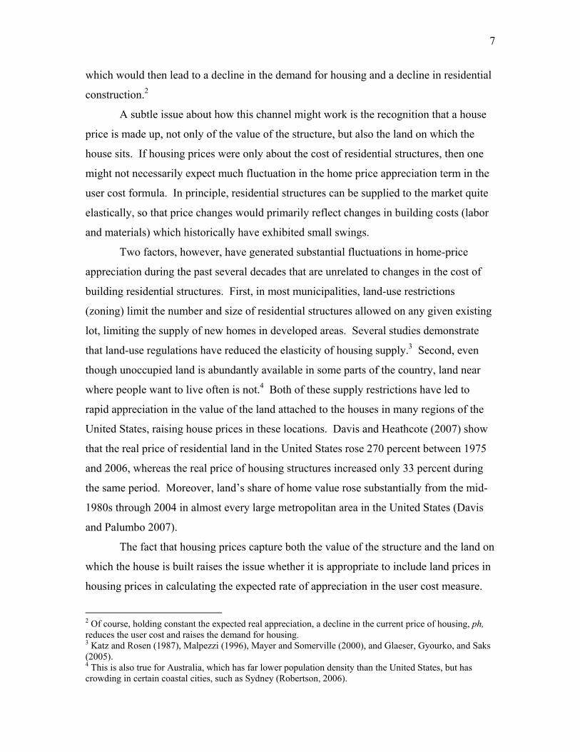
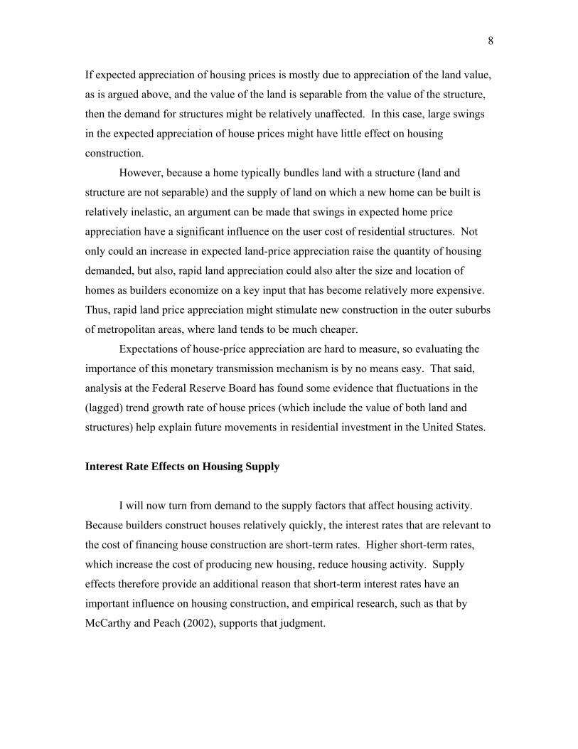
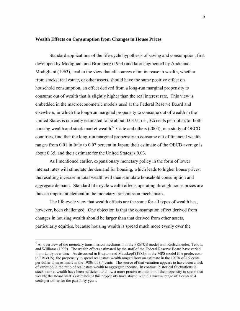
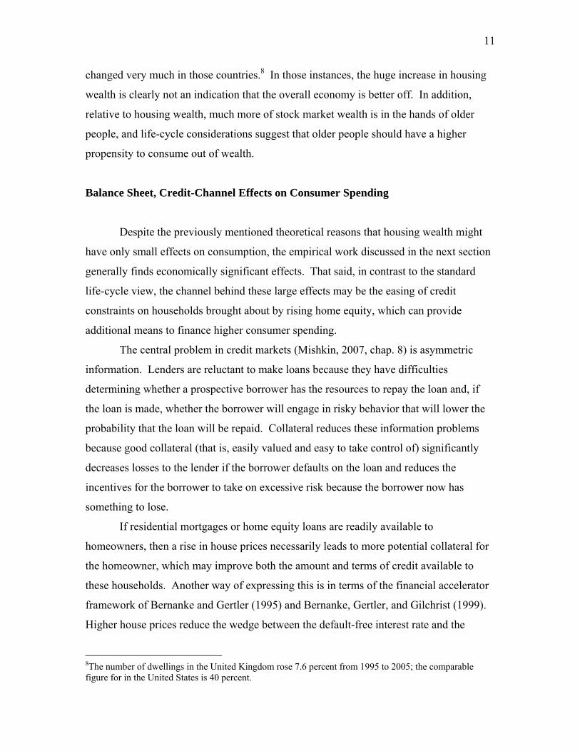
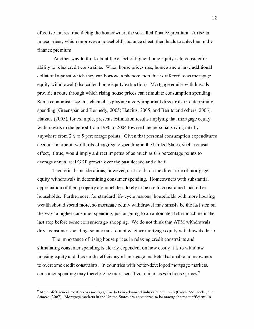
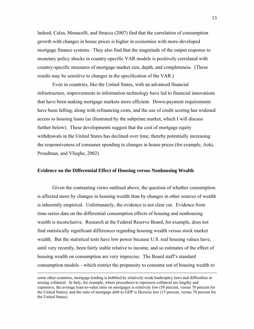
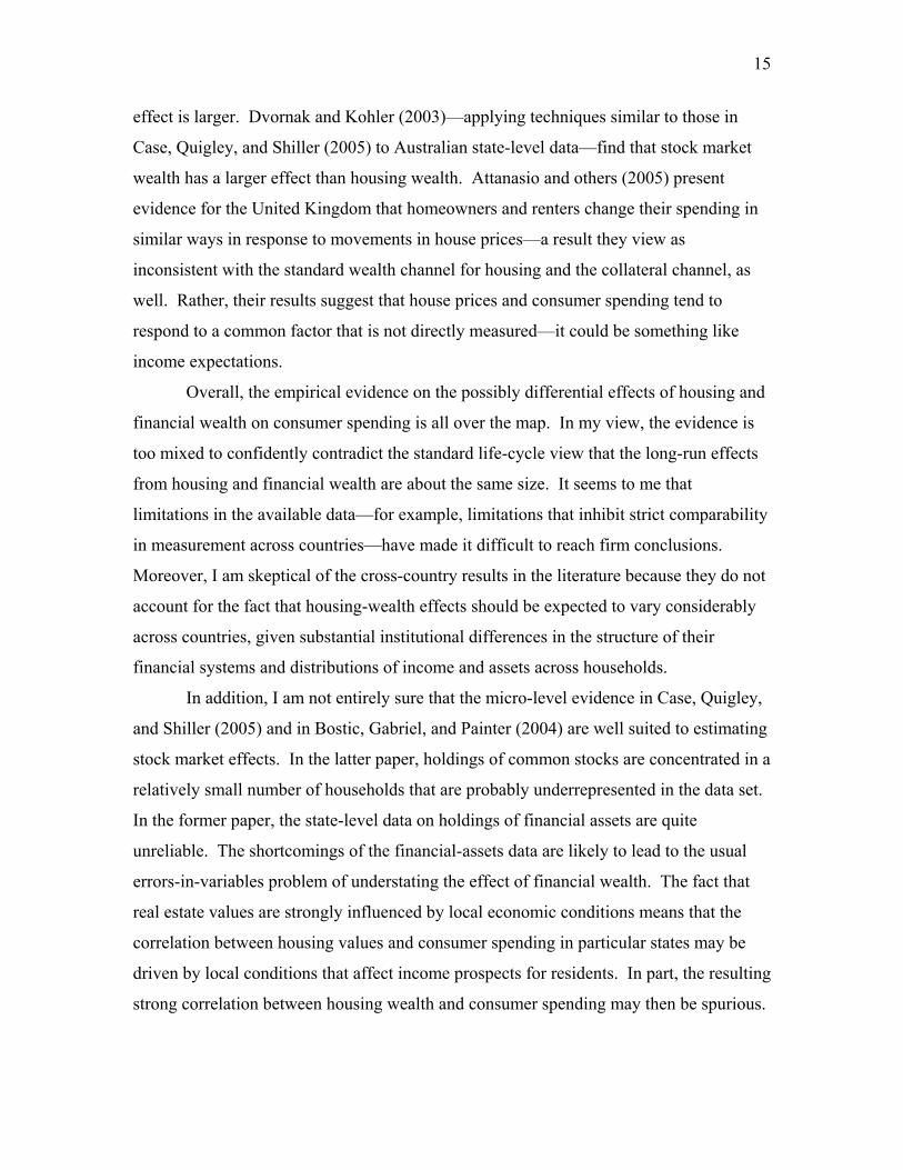
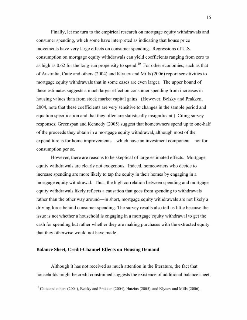
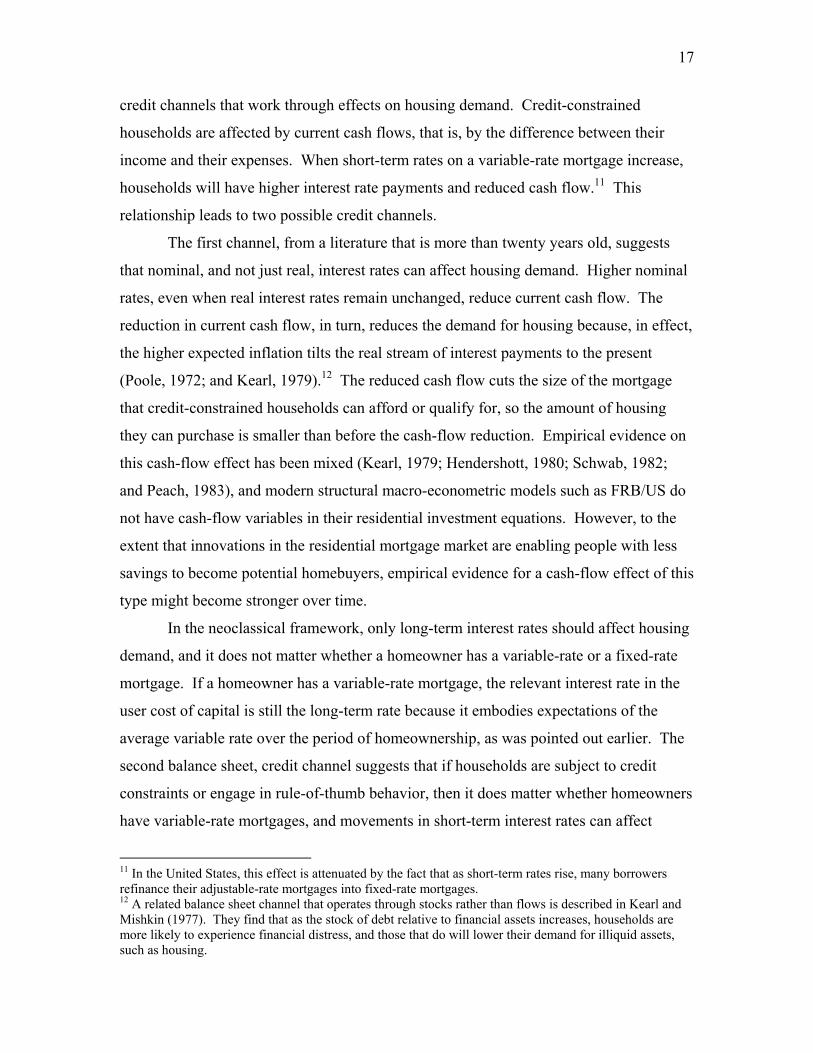
The big gains in housing prices we have seen here and in many other countries (figure 1)

have raised concerns about what might happen to economic activity if those price gains

are reversed. Developments in the housing market can also affect credit markets. In the

United States, rising delinquencies of subprime residential mortgages have led to

substantial losses to holders of securities backed by those mortgages and to sharp

increases in credit spreads for those securities. Furthermore, problems in the subprime

mortgage market have led investors to reassess credit risk and risk pricing, thereby

widening spreads in general and weakening the balance sheets of some financial

institutions. Fortunately, the overall financial system appears to be in good health, and

the U.S. banking system is well positioned to withstand stressful market conditions.

Given its important role in the economy, the housing market is of central concern

to monetary policy makers. To achieve the dual goals of promoting price stability and

maximum sustainable employment, monetary policy makers must understand the role

that housing plays in the monetary transmission mechanism if they are to appropriately

set policy instruments.

In this paper, I examine what we know about the role of housing in the monetary

transmission mechanism and then explore the implications of this knowledge for the

conduct of monetary policy.

2

AU

GU

ST

3, 2

007

Fig

ure

1:

Rea

l Ho

use

Pri

ces

in t

he

Ad

van

ced

Fo

reig

n E

con

om

ies

(Def

late

d w

ith C

PI;

Per

cent

cha

nge

from

yea

r ea

rlier

)

1995

2000

2005

-10

-4281420

*Est

ablis

hed

hom

es, w

eigh

ted

aver

age

of 8

citi

es.

Sour

ce: A

ustr

alia

n B

urea

u of

Sta

tistic

s.

Au

stra

lia*

Qua

rter

ly

1995

2000

2005

-10

-4281420

*Val

ue o

f ne

w h

ouse

s (i

nclu

ding

val

ue o

f lo

t),

surv

ey o

f 21

citi

es.

Sour

ce: S

tatis

tics

Can

ada.

Can

ada*

Mon

thly

1995

2000

2005

-10

-26142230

*Sin

gle-

fam

ily h

ouse

s. S

ourc

e: D

anm

arks

Sta

tistik

.

Den

mar

k*Q

uart

erly

1995

2000

2005

-10

-6-22610

*Res

iden

tial P

rope

rty

Pric

es.

Sour

ce: E

urop

ean

Cen

tral

Ban

k.

Eu

ro A

rea*

Sem

iann

ual

1995

2000

2005

-20

-12

-441220

*Det

ache

d H

ouse

s. S

ourc

e: S

tatis

tics

Finl

and.

Fin

lan

d*

Qua

rter

ly

1995

2000

2005

-30

-20

-1001020

*All

hous

ing

units

. So

urce

: IN

SEE

.

Fra

nce

*Q

uart

erly

3

AU

GU

ST

3, 2

007

Fig

ure

1:

Rea

l Ho

use

Pri

ces

in t

he

Ad

van

ced

Fo

reig

n E

con

om

ies

(Def

late

d w

ith C

PI;

Per

cent

cha

nge

from

yea

r ea

rlier

)

1995

2000

2005

-10

-6-22610

*Sou

rce:

Bul

wie

n A

G.

Sin

gle-

fam

ily h

omes

Ow

ner-

occu

pied

apa

rtm

ents

Ger

man

y*A

nnua

l

1995

2000

2005

-10

-4281420

*All

dwel

lings

in u

rban

are

as.

Sour

ce: B

ank

ofG

reec

e.

Gre

ece*

Qua

rter

ly

1995

2000

2005

-10

-26142230

*Sou

rce:

Dep

artm

ent o

f th

e E

nvir

onm

ent,

Her

itage

and

Loc

al G

over

nmen

t.

New

hou

ses

Exi

stin

g ho

uses

Irel

and

*Q

uart

erly

1995

2000

2005

-10

-8-6-4-20

*Urb

an r

esid

entia

l lan

d pr

ices

, sur

vey

of 2

23 c

ities

.So

urce

: Jap

an R

eal E

stat

e R

esea

rch

Inst

itute

.

Jap

an*

Sem

iann

ual

1995

2000

2005

-10

-4281420

*Sin

gle-

fam

ily h

omes

and

apa

rtm

ents

.So

urce

: Kad

aste

r, D

utch

Lan

d R

egis

try

Off

ice.

Net

her

lan

ds*

Mon

thly

1995

2000

2005

-10

-26142230

*All

hous

ehol

ds.

Sour

ce: R

eser

ve B

ank

of N

ewZ

eala

nd.

New

Zea

lan

d*

Qua

rter

ly

4

AU

GU

ST

3, 2

007

Fig

ure

1:

Rea

l Ho

use

Pri

ces

in t

he

Ad

van

ced

Fo

reig

n E

con

om

ies

(Def

late

d w

ith C

PI;

Per

cent

cha

nge

from

yea

r ea

rlier

)

1995

2000

2005

-10

-6-22610

*New

det

ache

d ho

uses

. So

urce

: Sta

tistik

Sen

tral

byra

.

No

rway

*Q

uart

erly

1995

2000

2005

-10

-4281420

*Non

-pro

tect

ed h

ousi

ng.

Sour

ce: M

inis

teri

o de

Viv

iend

a.

Sp

ain

*Q

uart

erly

1995

2000

2005

-30

-20

-1001020

*One

and

two-

dwel

ling

build

ings

for

per

man

ent

livin

g. S

ourc

e: S

tatis

tiska

Cen

tral

byra

n.

Sw

eden

*Q

uart

erly

1995

2000

2005

-14

-8-241016

*Sou

rce:

Sw

iss

Nat

iona

l Ban

k.

Sin

gle-

fam

ily h

omes

Ow

ner-

occu

pied

apt

s

Sw

itze

rlan

d*

Qua

rter

ly

1995

2000

2005

-20

-100102030

*Sou

rce:

Nat

ionw

ide

and

Hal

ifax

, tw

o of

Bri

tain

’sla

rges

t len

ders

.

Nat

ionw

ide

Hal

ifax

Un

ited

Kin

gd

om

*M

onth

ly

1995

2000

2005

-10

-6-22610

*Hou

se p

rice

inde

x, p

urch

ase

only

. So

urce

: OFH

EO

.

Un

ited

Sta

tes*

Qua

rter

ly

5

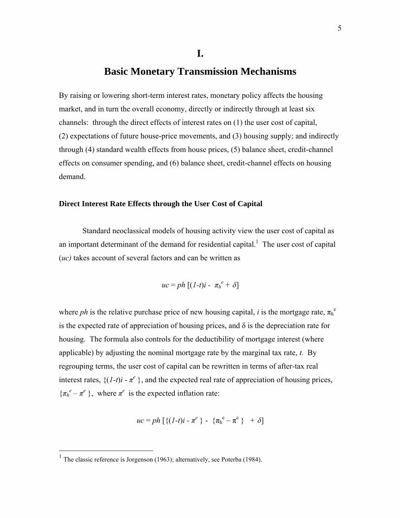
I.

Basic Monetary Transmission Mechanisms

By raising or lowering short-term interest rates, monetary policy affects the housing

market, and in turn the overall economy, directly or indirectly through at least six

channels: through the direct effects of interest rates on (1) the user cost of capital,

(2) expectations of future house-price movements, and (3) housing supply; and indirectly

through (4) standard wealth effects from house prices, (5) balance sheet, credit-channel

effects on consumer spending, and (6) balance sheet, credit-channel effects on housing

demand.

Direct Interest Rate Effects through the User Cost of Capital

Standard neoclassical models of housing activity view the user cost of capital as

an important determinant of the demand for residential capital.1 The user cost of capital

(uc) takes account of several factors and can be written as

uc = ph [(1-t)i - πhe + δ]

where ph is the relative purchase price of new housing capital, i is the mortgage rate, πhe

is the expected rate of appreciation of housing prices, and δ is the depreciation rate for

housing. The formula also controls for the deductibility of mortgage interest (where

applicable) by adjusting the nominal mortgage rate by the marginal tax rate, t. By

regrouping terms, the user cost of capital can be rewritten in terms of after-tax real

interest rates, {(1-t)i - πe }, and the expected real rate of appreciation of housing prices,

{πhe – πe }, where πe is the expected inflation rate:

uc = ph [{(1-t)i - πe } - {πhe – πe } + δ]

1 The classic reference is Jorgenson (1963); alternatively, see Poterba (1984).

6

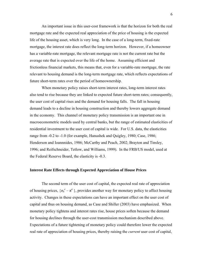
An important issue in this user-cost framework is that the horizon for both the real

mortgage rate and the expected real appreciation of the price of housing is the expected

life of the housing asset, which is very long. In the case of a long-term, fixed-rate

mortgage, the interest rate does reflect the long-term horizon. However, if a homeowner

has a variable-rate mortgage, the relevant mortgage rate is not the current rate but the

average rate that is expected over the life of the home. Assuming efficient and

frictionless financial markets, this means that, even for a variable-rate mortgage, the rate

relevant to housing demand is the long-term mortgage rate, which reflects expectations of

future short-term rates over the period of homeownership.

When monetary policy raises short-term interest rates, long-term interest rates

also tend to rise because they are linked to expected future short-term rates; consequently,

the user cost of capital rises and the demand for housing falls. The fall in housing

demand leads to a decline in housing construction and thereby lowers aggregate demand

in the economy. This channel of monetary policy transmission is an important one in

macroeconometric models used by central banks, but the range of estimated elasticities of

residential investment to the user cost of capital is wide. For U.S. data, the elasticities

range from -0.2 to -1.0 (for example, Hanushek and Quigley, 1980; Case, 1986;

Henderson and Ioannnides, 1986; McCarthy and Peach, 2002; Brayton and Tinsley,

1996; and Reifschneider, Tetlow, and Williams, 1999). In the FRB/US model, used at

the Federal Reserve Board, the elasticity is -0.3.

Interest Rate Effects through Expected Appreciation of House Prices

The second term of the user cost of capital, the expected real rate of appreciation

of housing prices, {πhe – πe }, provides another way for monetary policy to affect housing

activity. Changes in these expectations can have an important effect on the user cost of

capital and thus on housing demand, as Case and Shiller (2003) have emphasized. When

monetary policy tightens and interest rates rise, house prices soften because the demand

for housing declines through the user-cost transmission mechanism described above.

Expectations of a future tightening of monetary policy could therefore lower the expected

real rate of appreciation of housing prices, thereby raising the current user cost of capital,

7

which would then lead to a decline in the demand for housing and a decline in residential

construction.2

A subtle issue about how this channel might work is the recognition that a house

price is made up, not only of the value of the structure, but also the land on which the

house sits. If housing prices were only about the cost of residential structures, then one

might not necessarily expect much fluctuation in the home price appreciation term in the

user cost formula. In principle, residential structures can be supplied to the market quite

elastically, so that price changes would primarily reflect changes in building costs (labor

and materials) which historically have exhibited small swings.

Two factors, however, have generated substantial fluctuations in home-price

appreciation during the past several decades that are unrelated to changes in the cost of

building residential structures. First, in most municipalities, land-use restrictions

(zoning) limit the number and size of residential structures allowed on any given existing

lot, limiting the supply of new homes in developed areas. Several studies demonstrate

that land-use regulations have reduced the elasticity of housing supply.3 Second, even

though unoccupied land is abundantly available in some parts of the country, land near

where people want to live often is not.4 Both of these supply restrictions have led to

rapid appreciation in the value of the land attached to the houses in many regions of the

United States, raising house prices in these locations. Davis and Heathcote (2007) show

that the real price of residential land in the United States rose 270 percent between 1975

and 2006, whereas the real price of housing structures increased only 33 percent during

the same period. Moreover, land’s share of home value rose substantially from the mid-

1980s through 2004 in almost every large metropolitan area in the United States (Davis

and Palumbo 2007).

The fact that housing prices capture both the value of the structure and the land on

which the house is built raises the issue whether it is appropriate to include land prices in

housing prices in calculating the expected rate of appreciation in the user cost measure.

2 Of course, holding constant the expected real appreciation, a decline in the current price of housing, ph, reduces the user cost and raises the demand for housing. 3 Katz and Rosen (1987), Malpezzi (1996), Mayer and Somerville (2000), and Glaeser, Gyourko, and Saks (2005). 4 This is also true for Australia, which has far lower population density than the United States, but has crowding in certain coastal cities, such as Sydney (Robertson, 2006).

8

If expected appreciation of housing prices is mostly due to appreciation of the land value,

as is argued above, and the value of the land is separable from the value of the structure,

then the demand for structures might be relatively unaffected. In this case, large swings

in the expected appreciation of house prices might have little effect on housing

construction.

However, because a home typically bundles land with a structure (land and

structure are not separable) and the supply of land on which a new home can be built is

relatively inelastic, an argument can be made that swings in expected home price

appreciation have a significant influence on the user cost of residential structures. Not

only could an increase in expected land-price appreciation raise the quantity of housing

demanded, but also, rapid land appreciation could also alter the size and location of

homes as builders economize on a key input that has become relatively more expensive.

Thus, rapid land price appreciation might stimulate new construction in the outer suburbs

of metropolitan areas, where land tends to be much cheaper.

Expectations of house-price appreciation are hard to measure, so evaluating the

importance of this monetary transmission mechanism is by no means easy. That said,

analysis at the Federal Reserve Board has found some evidence that fluctuations in the

(lagged) trend growth rate of house prices (which include the value of both land and

structures) help explain future movements in residential investment in the United States.

Interest Rate Effects on Housing Supply

I will now turn from demand to the supply factors that affect housing activity.

Because builders construct houses relatively quickly, the interest rates that are relevant to

the cost of financing house construction are short-term rates. Higher short-term rates,

which increase the cost of producing new housing, reduce housing activity. Supply

effects therefore provide an additional reason that short-term interest rates have an

important influence on housing construction, and empirical research, such as that by

McCarthy and Peach (2002), supports that judgment.

9

Wealth Effects on Consumption from Changes in House Prices

Standard applications of the life-cycle hypothesis of saving and consumption, first

developed by Modigliani and Brumberg (1954) and later augmented by Ando and

Modigliani (1963), lead to the view that all sources of an increase in wealth, whether

from stocks, real estate, or other assets, should have the same positive effect on

household consumption, an effect derived from a long-run marginal propensity to

consume out of wealth that is slightly higher than the real interest rate. This view is

embedded in the macroeconometric models used at the Federal Reserve Board and

elsewhere, in which the long-run marginal propensity to consume out of wealth in the

United States is currently estimated to be about 0.0375, i.e., 3¾ cents per dollar,for both

housing wealth and stock market wealth.5 Catte and others (2004), in a study of OECD

countries, find that the long-run marginal propensity to consume out of financial wealth

ranges from 0.01 in Italy to 0.07 percent in Japan; their estimate of the OECD average is

about 0.35, and their estimate for the United States is 0.03.

As I mentioned earlier, expansionary monetary policy in the form of lower

interest rates will stimulate the demand for housing, which leads to higher house prices;

the resulting increase in total wealth will then stimulate household consumption and

aggregate demand. Standard life-cycle wealth effects operating through house prices are

thus an important element in the monetary transmission mechanism.

The life-cycle view that wealth effects are the same for all types of wealth has,

however, been challenged. One objection is that the consumption effect derived from

changes in housing wealth should be larger than that derived from other assets,

particularly equities, because housing wealth is spread much more evenly over the

5 An overview of the monetary transmission mechanism in the FRB/US model is in Reifschneider, Tetlow, and Williams (1999). The wealth effects estimated by the staff of the Federal Reserve Board have varied importantly over time. As discussed in Brayton and Mauskopf (1985), in the MPS model (the predecessor to FRB/US), the propensity to spend real estate wealth ranged from an estimate in the 1970s of 2.9 cents per dollar to an estimate in the 1980s of 8.4 cents. The source of that variation appears to have been a lack of variation in the ratio of real estate wealth to aggregate income. In contrast, historical fluctuations in stock market wealth have been sufficient to allow a more precise estimation of the propensity to spend that wealth; the Board staff’s estimates of this propensity have stayed within a narrow range of 3 cents to 4 cents per dollar for the past forty years.

10

population than is stock market wealth.6 If the marginal propensity to consume out of

wealth is lower for the rich, as economic theory and empirical evidence suggest (Lusardi,

1996; and Souleles, 1999), then changes in housing wealth might have a larger effect on

consumption than changes in stock market wealth. In addition, because house prices are

much less volatile than stock prices, changes in housing wealth might be viewed as much

longer lasting than changes in stock market wealth, another reason that housing wealth

should have a greater effect on consumption than stock market wealth.

Another challenge to the life-cycle view would work through a bequest motive,

leading one to think that the consumption effect derived from housing wealth could be

smaller than that derived from other assets. Consider a case in which homeowners plan

to live in their house (or an equivalent one) until they die, plan to pass on their home to

their children as a bequest, and value their children’s utility as much as their own. For

such homeowners, a rise in wealth from an increase in the value of their home will be

matched by an increase in the implicit cost of living in their house (their consumption of

housing services); thus, an increase in the value of their home should not raise their

nonhousing spending.7 Higher house prices could even reduce current consumption for

those planning to buy a house if they believe they will need to save more to do so. The

consumption effect of rising house prices is thus uncertain and subject to distributional

effects, depending on who is getting the increased housing wealth.

Another reason that increases in housing wealth might have a smaller effect on

consumption than increases in stock market wealth is that the latter are more clearly

connected than the former to future increases in the productive potential of the economy.

The possibility that rising house prices might not reflect an increase in future productivity

is supported by the recognition that, as mentioned earlier, rising house prices may

primarily be the result of supply constraints in the housing market. For example, supply

restrictions have been very severe in some countries, such as the United Kingdom, that

have had the largest appreciation in real house prices, so the actual housing stock has not

6 In the United States in 2001, for example, the top 1 percent of stockholders held one-third of total stock market wealth, while the top 1 percent of homeowners held only one-eighth of housing wealth (Belsky and Prakken, 2004). 7 Clearly, for older homeowners who plan to sell or downsize their houses in the near future, the increased wealth from higher house prices gives them more resources with which to increase their consumption spending.

11

changed very much in those countries.8 In those instances, the huge increase in housing

wealth is clearly not an indication that the overall economy is better off. In addition,

relative to housing wealth, much more of stock market wealth is in the hands of older

people, and life-cycle considerations suggest that older people should have a higher

propensity to consume out of wealth.

Balance Sheet, Credit-Channel Effects on Consumer Spending

Despite the previously mentioned theoretical reasons that housing wealth might

have only small effects on consumption, the empirical work discussed in the next section

generally finds economically significant effects. That said, in contrast to the standard

life-cycle view, the channel behind these large effects may be the easing of credit

constraints on households brought about by rising home equity, which can provide

additional means to finance higher consumer spending.

The central problem in credit markets (Mishkin, 2007, chap. 8) is asymmetric

information. Lenders are reluctant to make loans because they have difficulties

determining whether a prospective borrower has the resources to repay the loan and, if

the loan is made, whether the borrower will engage in risky behavior that will lower the

probability that the loan will be repaid. Collateral reduces these information problems

because good collateral (that is, easily valued and easy to take control of) significantly

decreases losses to the lender if the borrower defaults on the loan and reduces the

incentives for the borrower to take on excessive risk because the borrower now has

something to lose.

If residential mortgages or home equity loans are readily available to

homeowners, then a rise in house prices necessarily leads to more potential collateral for

the homeowner, which may improve both the amount and terms of credit available to

these households. Another way of expressing this is in terms of the financial accelerator

framework of Bernanke and Gertler (1995) and Bernanke, Gertler, and Gilchrist (1999).

Higher house prices reduce the wedge between the default-free interest rate and the

8The number of dwellings in the United Kingdom rose 7.6 percent from 1995 to 2005; the comparable figure for in the United States is 40 percent.

12

effective interest rate facing the homeowner, the so-called finance premium. A rise in

house prices, which improves a household’s balance sheet, then leads to a decline in the

finance premium.

Another way to think about the effect of higher home equity is to consider its

ability to relax credit constraints. When house prices rise, homeowners have additional

collateral against which they can borrow, a phenomenon that is referred to as mortgage

equity withdrawal (also called home equity extraction). Mortgage equity withdrawals

provide a route through which rising house prices can stimulate consumption spending.

Some economists see this channel as playing a very important direct role in determining

spending (Greenspan and Kennedy, 2005; Hatzius, 2005; and Benito and others, 2006).

Hatzius (2005), for example, presents estimation results implying that mortgage equity

withdrawals in the period from 1990 to 2004 lowered the personal saving rate by

anywhere from 2½ to 5 percentage points. Given that personal consumption expenditures

account for about two-thirds of aggregate spending in the United States, such a causal

effect, if true, would imply a direct impetus of as much as 0.3 percentage points to

average annual real GDP growth over the past decade and a half.

Theoretical considerations, however, cast doubt on the direct role of mortgage

equity withdrawals in determining consumer spending. Homeowners with substantial

appreciation of their property are much less likely to be credit constrained than other

households. Furthermore, for standard life-cycle reasons, households with more housing

wealth should spend more, so mortgage equity withdrawal may simply be the last step on

the way to higher consumer spending, just as going to an automated teller machine is the

last step before some consumers go shopping. We do not think that ATM withdrawals

drive consumer spending, so one must doubt whether mortgage equity withdrawals do so.

The importance of rising house prices in relaxing credit constraints and

stimulating consumer spending is clearly dependent on how costly it is to withdraw

housing equity and thus on the efficiency of mortgage markets that enable homeowners

to overcome credit constraints. In countries with better-developed mortgage markets,

consumer spending may therefore be more sensitive to increases in house prices.9

9 Major differences exist across mortgage markets in advanced industrial countries (Calza, Monacelli, and Stracca, 2007). Mortgage markets in the United States are considered to be among the most efficient; in

13

Indeed, Calza, Monacelli, and Stracca (2007) find that the correlation of consumption

growth with changes in house prices is higher in economies with more-developed

mortgage finance systems. They also find that the magnitude of the output response to

monetary policy shocks in country-specific VAR models is positively correlated with

country-specific measures of mortgage market size, depth, and completeness. (These

results may be sensitive to changes in the specification of the VAR.)

Even in countries, like the United States, with an advanced financial

infrastructure, improvements in information technology have led to financial innovations

that have been making mortgage markets more efficient. Down-payment requirements

have been falling, along with refinancing costs, and the use of credit scoring has widened

access to housing loans (as illustrated by the subprime market, which I will discuss

further below). These developments suggest that the cost of mortgage equity

withdrawals in the United States has declined over time, thereby potentially increasing

the responsiveness of consumer spending to changes in house prices (for example, Aoki,

Proudman, and Vlieghe, 2002).

Evidence on the Differential Effect of Housing versus Nonhousing Wealth

Given the contrasting views outlined above, the question of whether consumption

is affected more by changes in housing wealth than by changes in other sources of wealth

is inherently empirical. Unfortunately, the evidence is not clear cut. Evidence from

time-series data on the differential consumption effects of housing and nonhousing

wealth is inconclusive. Research at the Federal Reserve Board, for example, does not

find statistically significant differences regarding housing wealth versus stock market

wealth. But the statistical tests have low power because U.S. real housing values have,

until very recently, been fairly stable relative to income, and so estimates of the effect of

housing wealth on consumption are very imprecise. The Board staff’s standard

consumption models—which restrict the propensity to consume out of housing wealth to some other countries, mortgage lending is hobbled by relatively weak bankruptcy laws and difficulties in seizing collateral. In Italy, for example, where procedures to repossess collateral are lengthy and expensive, the average loan-to-value ratio on mortgages is relatively low (50 percent, versus 70 percent for the United States), and the ratio of mortgage debt to GDP is likewise low (15 percent, versus 70 percent for the United States).

14

equal the propensity to consume out of nonhousing wealth—continue to track aggregate

consumption spending well, even when the models are estimated with data ending in

1995. Thus, these models do not suggest that an increased sensitivity of consumption to

housing wealth is needed to explain the low rates of personal saving in recent years. Like

the Board staff, Belsky and Prakken (2004) have found that the propensities to consume

housing and financial wealth are about the same in the long run; however, Belsky and

Prakken (2004) estimate that spending reacts to housing wealth more quickly than it does

to financial wealth.

Other research is more favorable to the view that housing wealth has a larger

long-run effect on consumer spending that does stock market wealth. In general, research

based on pooled cross-country time-series data tends to be more favorable to the view

that housing wealth has a greater effect on consumer spending than does stock market

wealth. Case, Quigley, and Shiller (2005) find that the elasticity of consumer spending to

housing wealth is between 11 percent and 17 percent, while it is only 2 percent for stock

market wealth. Bayoumi and Edison (2003) find that the marginal propensity to consume

out of a dollar increase in housing wealth is 7 cents, while it is 4½ cents for stock market

wealth. Ludwig and Slok (2002) find that effects from housing wealth exceed those from

stock market wealth in the sixteen OECD countries they examine and that the difference

has been growing. Case, Quigley, and Shiller (2005), who conduct a similar analysis on

state-level data for the United States, find that the elasticity of consumer spending to

housing wealth is between 5 percent and 9 percent, while the elasticity with respect to

stock market wealth is not statistically different from zero. In addition, Carroll, Otsuka,

and Slacalek (2006), using time-series data for just the United States, estimate that the

long-run marginal propensity to consume out of a dollar increase in housing wealth is 9

cents, compared with 4 cents for nonhousing wealth. Finally, using household-level data

for the United States, Bostic, Gabriel, and Painter (2004) estimate that consumer

spending is twice as sensitive to changes in housing wealth as it is to financial wealth.

There is also a body of empirical research that reports results less favorable to the

view that housing wealth has a bigger effect on consumer spending than does stock

market wealth. Girouard and Blondal (2001) do not find consistent results across

countries: In some countries the stock market effect is larger, while in others the housing

15

effect is larger. Dvornak and Kohler (2003)—applying techniques similar to those in

Case, Quigley, and Shiller (2005) to Australian state-level data—find that stock market

wealth has a larger effect than housing wealth. Attanasio and others (2005) present

evidence for the United Kingdom that homeowners and renters change their spending in

similar ways in response to movements in house prices—a result they view as

inconsistent with the standard wealth channel for housing and the collateral channel, as

well. Rather, their results suggest that house prices and consumer spending tend to

respond to a common factor that is not directly measured—it could be something like

income expectations.

Overall, the empirical evidence on the possibly differential effects of housing and

financial wealth on consumer spending is all over the map. In my view, the evidence is

too mixed to confidently contradict the standard life-cycle view that the long-run effects

from housing and financial wealth are about the same size. It seems to me that

limitations in the available data—for example, limitations that inhibit strict comparability

in measurement across countries—have made it difficult to reach firm conclusions.

Moreover, I am skeptical of the cross-country results in the literature because they do not

account for the fact that housing-wealth effects should be expected to vary considerably

across countries, given substantial institutional differences in the structure of their

financial systems and distributions of income and assets across households.

In addition, I am not entirely sure that the micro-level evidence in Case, Quigley,

and Shiller (2005) and in Bostic, Gabriel, and Painter (2004) are well suited to estimating

stock market effects. In the latter paper, holdings of common stocks are concentrated in a

relatively small number of households that are probably underrepresented in the data set.

In the former paper, the state-level data on holdings of financial assets are quite

unreliable. The shortcomings of the financial-assets data are likely to lead to the usual

errors-in-variables problem of understating the effect of financial wealth. The fact that

real estate values are strongly influenced by local economic conditions means that the

correlation between housing values and consumer spending in particular states may be

driven by local conditions that affect income prospects for residents. In part, the resulting

strong correlation between housing wealth and consumer spending may then be spurious.

16

Finally, let me turn to the empirical research on mortgage equity withdrawals and

consumer spending, which some have interpreted as indicating that house price

movements have very large effects on consumer spending. Regressions of U.S.

consumption on mortgage equity withdrawals can yield coefficients ranging from zero to

as high as 0.62 for the long-run propensity to spend.10 For other economies, such as that

of Australia, Catte and others (2004) and Klyuev and Mills (2006) report sensitivities to

mortgage equity withdrawals that in some cases are even larger. The upper bound of

these estimates suggests a much larger effect on consumer spending from increases in

housing values than from stock market capital gains. (However, Belsky and Prakken,

2004, note that these coefficients are very sensitive to changes in the sample period and

equation specification and that they often are statistically insignificant.) Citing survey

responses, Greenspan and Kennedy (2005) suggest that homeowners spend up to one-half

of the proceeds they obtain in a mortgage equity withdrawal, although most of the

expenditure is for home improvements—which have an investment component—not for

consumption per se.

However, there are reasons to be skeptical of large estimated effects. Mortgage

equity withdrawals are clearly not exogenous. Indeed, homeowners who decide to

increase spending are more likely to tap the equity in their homes by engaging in a

mortgage equity withdrawal. Thus, the high correlation between spending and mortgage

equity withdrawals likely reflects a causation that goes from spending to withdrawals

rather than the other way around—in short, mortgage equity withdrawals are not likely a

driving force behind consumer spending. The survey results also tell us little because the

issue is not whether a household is engaging in a mortgage equity withdrawal to get the

cash for spending but rather whether they are making purchases with the extracted equity

that they otherwise would not have made.

Balance Sheet, Credit-Channel Effects on Housing Demand

Although it has not received as much attention in the literature, the fact that

households might be credit constrained suggests the existence of additional balance sheet,

10 Catte and others (2004), Belsky and Prakken (2004), Hatzius (2005), and Klyuev and Mills (2006).

17

credit channels that work through effects on housing demand. Credit-constrained

households are affected by current cash flows, that is, by the difference between their

income and their expenses. When short-term rates on a variable-rate mortgage increase,

households will have higher interest rate payments and reduced cash flow.11 This

relationship leads to two possible credit channels.

The first channel, from a literature that is more than twenty years old, suggests

that nominal, and not just real, interest rates can affect housing demand. Higher nominal

rates, even when real interest rates remain unchanged, reduce current cash flow. The

reduction in current cash flow, in turn, reduces the demand for housing because, in effect,

the higher expected inflation tilts the real stream of interest payments to the present

(Poole, 1972; and Kearl, 1979).12 The reduced cash flow cuts the size of the mortgage

that credit-constrained households can afford or qualify for, so the amount of housing

they can purchase is smaller than before the cash-flow reduction. Empirical evidence on

this cash-flow effect has been mixed (Kearl, 1979; Hendershott, 1980; Schwab, 1982;

and Peach, 1983), and modern structural macro-econometric models such as FRB/US do

not have cash-flow variables in their residential investment equations. However, to the

extent that innovations in the residential mortgage market are enabling people with less

savings to become potential homebuyers, empirical evidence for a cash-flow effect of this

type might become stronger over time.

In the neoclassical framework, only long-term interest rates should affect housing

demand, and it does not matter whether a homeowner has a variable-rate or a fixed-rate

mortgage. If a homeowner has a variable-rate mortgage, the relevant interest rate in the

user cost of capital is still the long-term rate because it embodies expectations of the

average variable rate over the period of homeownership, as was pointed out earlier. The

second balance sheet, credit channel suggests that if households are subject to credit

constraints or engage in rule-of-thumb behavior, then it does matter whether homeowners

have variable-rate mortgages, and movements in short-term interest rates can affect

11 In the United States, this effect is attenuated by the fact that as short-term rates rise, many borrowers refinance their adjustable-rate mortgages into fixed-rate mortgages. 12 A related balance sheet channel that operates through stocks rather than flows is described in Kearl and Mishkin (1977). They find that as the stock of debt relative to financial assets increases, households are more likely to experience financial distress, and those that do will lower their demand for illiquid assets, such as housing.

18

housing demand. When short-term rates on a variable-rate mortgage are higher, credit-

constrained households will have higher interest rate payments and less cash flow and,

again, the size of the mortgage they will be able to afford, or qualify for, will be reduced.

If a large proportion of households purchase houses with variable-rate mortgages, then an

increase in short-term rates, even with long-rates unchanged or increasing less, can

significantly affect housing demand. Given that variable mortgage rates tend to move

more with the short-term interest rates that monetary policy makers use as their policy

instrument, countries with a higher proportion of households using variable-rate

mortgages could have a large response to changes in monetary policy.

As documented in Calza, Monacelli, and Stracca (2007), different institutional

features of residential mortgage markets in OECD countries lead to differing degrees of

adjustability of mortgage interest rates. These researchers classify interest rate

adjustments on residential mortgages in three categories: fixed, in which interest rates

are fixed for more than five years or until expiry; mixed, in which interest rates are fixed

for one to five years; and variable, in which interest rates are renegotiable after one year,

or tied to market rates, or adjustable at the discretion of the lender. For the United States,

they estimate that 85 percent of residential mortgages are fixed, 15 percent are mixed,

and none are variable. The United States has the highest percentage of fixed-rate

mortgages, but a number of other countries also issue mostly fixed-rate and mixed

mortgages, among them Belgium, Denmark, Germany, Spain, France, the Netherlands,

Austria, and Canada. Countries with mostly variable-rate mortgages include Greece,

Ireland, Luxembourg, Portugal, Finland, Australia, and the United Kingdom.13

Given the above reasoning, we might expect that, in countries with a higher share

of variable-rate mortgages, residential construction would be more sensitive to changes in

short-term interest rates and have a more powerful monetary transmission mechanism in

general (as conjectured by Debelle, 2004). We might also expect that countries with

higher proportions of variable-rate mortgages would experience more volatility in

housing activity. Although I am unaware of any direct evidence for a link between the

proportion of variable-rate mortgages and residential investment volatility—in fact, IMF

13 Japan is listed as having 64 percent of mortgages mixed and variable and 36 percent fixed; Italy is listed as having mostly mixed mortgages and 28 percent fixed (table 1 in Calza, Monacelli, and Stracca, 2007).

19

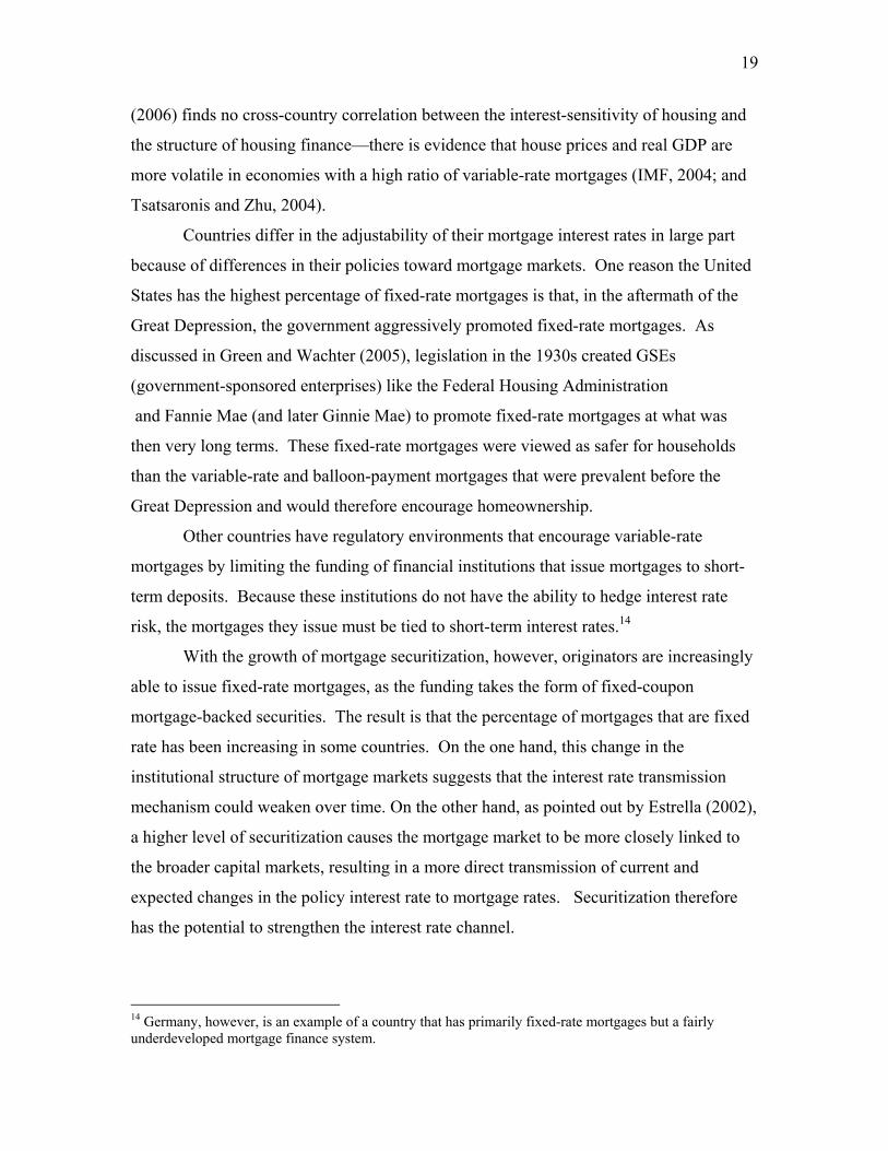
(2006) finds no cross-country correlation between the interest-sensitivity of housing and

the structure of housing finance—there is evidence that house prices and real GDP are

more volatile in economies with a high ratio of variable-rate mortgages (IMF, 2004; and

Tsatsaronis and Zhu, 2004).

Countries differ in the adjustability of their mortgage interest rates in large part

because of differences in their policies toward mortgage markets. One reason the United

States has the highest percentage of fixed-rate mortgages is that, in the aftermath of the

Great Depression, the government aggressively promoted fixed-rate mortgages. As

discussed in Green and Wachter (2005), legislation in the 1930s created GSEs

(government-sponsored enterprises) like the Federal Housing Administration

and Fannie Mae (and later Ginnie Mae) to promote fixed-rate mortgages at what was

then very long terms. These fixed-rate mortgages were viewed as safer for households

than the variable-rate and balloon-payment mortgages that were prevalent before the

Great Depression and would therefore encourage homeownership.

Other countries have regulatory environments that encourage variable-rate

mortgages by limiting the funding of financial institutions that issue mortgages to short-

term deposits. Because these institutions do not have the ability to hedge interest rate

risk, the mortgages they issue must be tied to short-term interest rates.14

With the growth of mortgage securitization, however, originators are increasingly

able to issue fixed-rate mortgages, as the funding takes the form of fixed-coupon

mortgage-backed securities. The result is that the percentage of mortgages that are fixed

rate has been increasing in some countries. On the one hand, this change in the

institutional structure of mortgage markets suggests that the interest rate transmission

mechanism could weaken over time. On the other hand, as pointed out by Estrella (2002),

a higher level of securitization causes the mortgage market to be more closely linked to

the broader capital markets, resulting in a more direct transmission of current and

expected changes in the policy interest rate to mortgage rates. Securitization therefore

has the potential to strengthen the interest rate channel.

14 Germany, however, is an example of a country that has primarily fixed-rate mortgages but a fairly underdeveloped mortgage finance system.

20

How Important is Housing in the Monetary Transmission Mechanism?

To get a feel for the role that housing plays in the monetary transmission

mechanism, we can look at simulations of macroeconometric models used by central

banks. The main macroeconometric model used at the Federal Reserve Board is the

FRB/US model. Although FRB/US does not include all the transmission mechanisms

outlined above, it does incorporate direct interest rate effects on housing activity through

the user cost of capital and through wealth (and possibly credit-channel) effects from

house prices, where the effects of housing and financial wealth are constrained to be

identical. To illustrate how important these transmission mechanisms are, we can ask

how this model responds to a monetary policy shock when the direct interest rate effect

on housing and the housing-wealth effects are shut down.

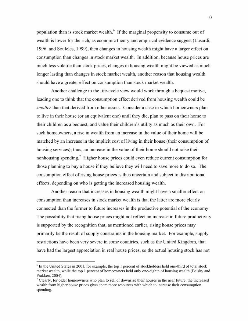
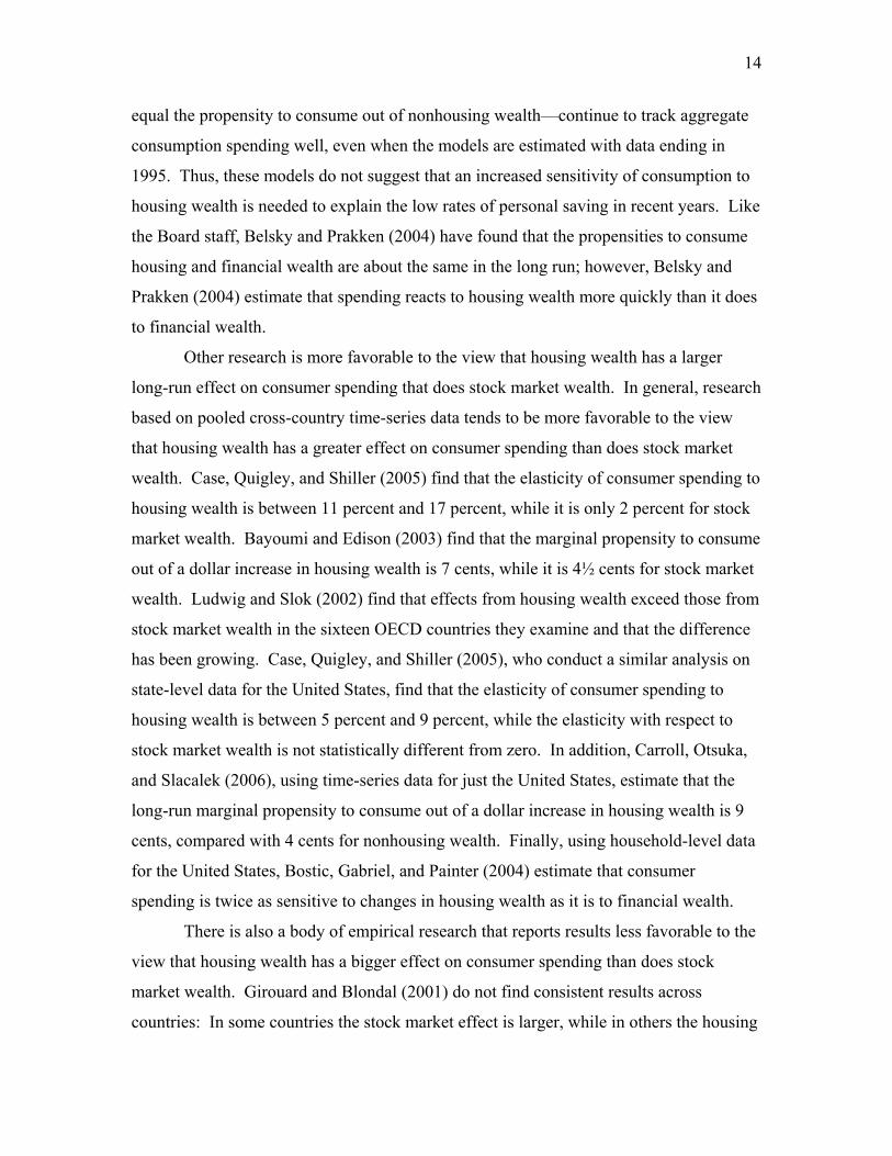
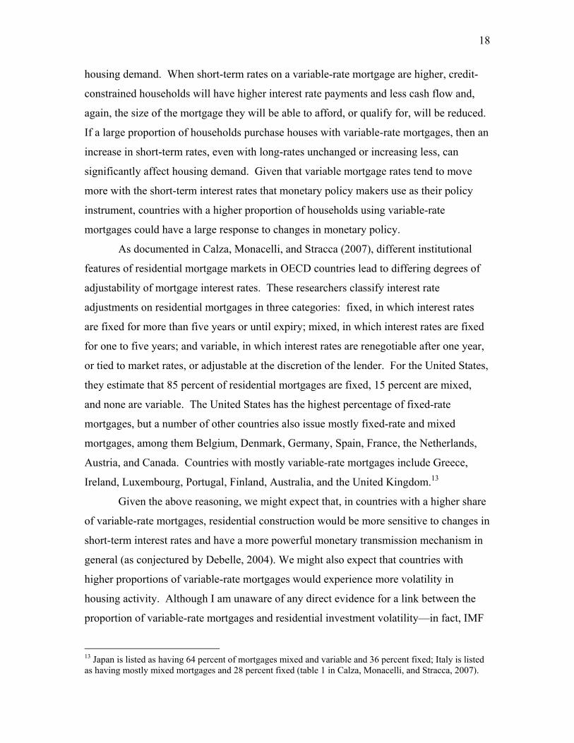
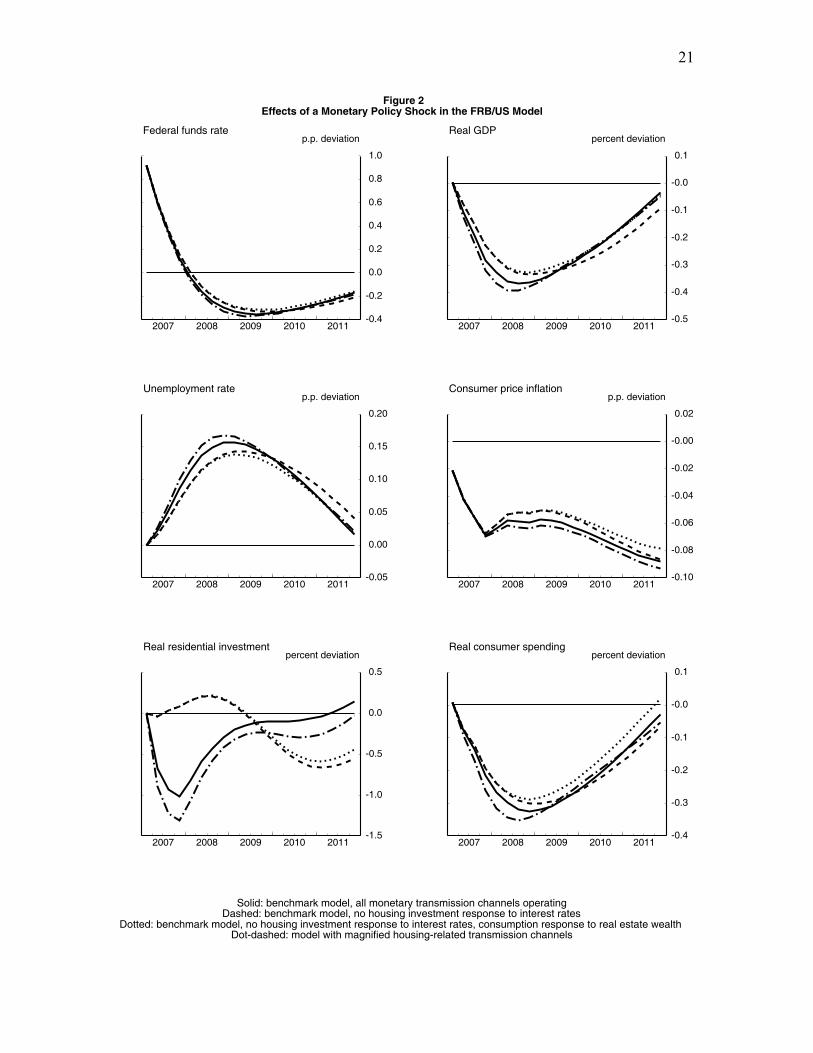
Figure 2 shows these simulations, with a 1 percentage point shock to the Taylor

rule for the federal funds rate, estimated over the 1987 to 2005 period, starting at the

beginning of 2007. The solid lines in this figure report the effects on the economy with

all housing-related transmission mechanisms operating. The dashed lines show the

effects when the direct effects of interest rates on residential investment are not operating,

and the dotted lines show the effect when the housing-wealth channel is also shut down.

As can be seen in the figure, shutting down these channels reduces the peak GDP

response by about 5 basis points, or 14 percent of the total response, which indicates that

the housing sector plays a moderate role in the transmission mechanism. However,

residential investment accounts for only 5 percent of GDP, so these simulation results

indicate that the sector is about three times more responsive to monetary policy in the

short run than is overall spending.

As the above survey of empirical evidence on the transmission mechanisms

suggests, the strength of the direct interest-rate and housing-wealth-effect channels is

subject to a great deal of uncertainty. As shown by the dotted-dashed line in figure 2, the

economy responds to the monetary policy shock when the two channels are magnified in

21

Figure 2Effects of a Monetary Policy Shock in the FRB/US Model

Solid: benchmark model, all monetary transmission channels operatingDashed: benchmark model, no housing investment response to interest rates

Dotted: benchmark model, no housing investment response to interest rates, consumption response to real estate wealthDot-dashed: model with magnified housing-related transmission channels

2007 2008 2009 2010 2011-0.4

-0.2

0.0

0.2

0.4

0.6

0.8

1.0

-0.4

-0.2

0.0

0.2

0.4

0.6

0.8

1.0

p.p. deviation

Federal funds rate

2007 2008 2009 2010 2011-0.5

-0.4

-0.3

-0.2

-0.1

-0.0

0.1

-0.5

-0.4

-0.3

-0.2

-0.1

-0.0

0.1

percent deviation

Real GDP

2007 2008 2009 2010 2011-0.05

0.00

0.05

0.10

0.15

0.20

-0.05

0.00

0.05

0.10

0.15

0.20

p.p. deviation

Unemployment rate

2007 2008 2009 2010 2011-0.10

-0.08

-0.06

-0.04

-0.02

-0.00

0.02

-0.10

-0.08

-0.06

-0.04

-0.02

-0.00

0.02

p.p. deviation

Consumer price inflation

2007 2008 2009 2010 2011-1.5

-1.0

-0.5

0.0

0.5

-1.5

-1.0

-0.5

0.0

0.5

percent deviation

Real residential investment

2007 2008 2009 2010 2011-0.4

-0.3

-0.2

-0.1

-0.0

0.1

-0.4

-0.3

-0.2

-0.1

-0.0

0.1

percent deviation

Real consumer spending

22

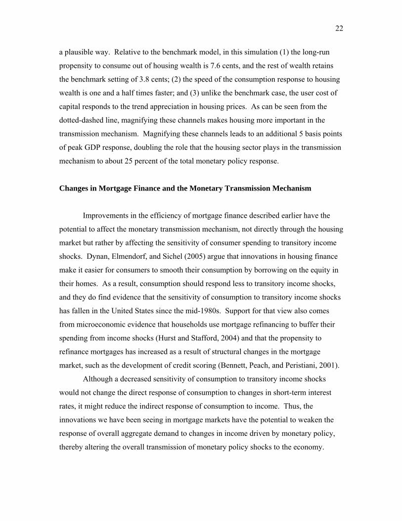
a plausible way. Relative to the benchmark model, in this simulation (1) the long-run

propensity to consume out of housing wealth is 7.6 cents, and the rest of wealth retains

the benchmark setting of 3.8 cents; (2) the speed of the consumption response to housing

wealth is one and a half times faster; and (3) unlike the benchmark case, the user cost of

capital responds to the trend appreciation in housing prices. As can be seen from the

dotted-dashed line, magnifying these channels makes housing more important in the

transmission mechanism. Magnifying these channels leads to an additional 5 basis points

of peak GDP response, doubling the role that the housing sector plays in the transmission

mechanism to about 25 percent of the total monetary policy response.

Changes in Mortgage Finance and the Monetary Transmission Mechanism

Improvements in the efficiency of mortgage finance described earlier have the

potential to affect the monetary transmission mechanism, not directly through the housing

market but rather by affecting the sensitivity of consumer spending to transitory income

shocks. Dynan, Elmendorf, and Sichel (2005) argue that innovations in housing finance

make it easier for consumers to smooth their consumption by borrowing on the equity in

their homes. As a result, consumption should respond less to transitory income shocks,

and they do find evidence that the sensitivity of consumption to transitory income shocks

has fallen in the United States since the mid-1980s. Support for that view also comes

from microeconomic evidence that households use mortgage refinancing to buffer their

spending from income shocks (Hurst and Stafford, 2004) and that the propensity to

refinance mortgages has increased as a result of structural changes in the mortgage

market, such as the development of credit scoring (Bennett, Peach, and Peristiani, 2001).

Although a decreased sensitivity of consumption to transitory income shocks

would not change the direct response of consumption to changes in short-term interest

rates, it might reduce the indirect response of consumption to income. Thus, the

innovations we have been seeing in mortgage markets have the potential to weaken the

response of overall aggregate demand to changes in income driven by monetary policy,

thereby altering the overall transmission of monetary policy shocks to the economy.

23

II. Financial Stability and the Monetary Transmission

Mechanism

So far, I have discussed monetary transmission mechanisms working through the

housing sector when the financial system is operating normally. However, exceptionally

unfavorable conditions in the housing sector have the potential to create instability in the

financial system—instability that could magnify problems for the overall economy. Two

questions thus arise: Through what channels might the housing sector at times be a

source of financial instability? And could such instability affect the operation of the

transmission mechanism, affecting the ability of a central bank to stabilize the overall

macroeconomy?

A breakdown in financial stability occurs when shocks to the financial system

cause disruptions to the credit intermediaries that are so severe that the system can no

longer channel funds fluidly to creditworthy households and businesses with productive

investment opportunities. Without access to financing, individuals and firms must cut

their spending, which will have consequences for overall economic activity.

As I noted in my 1997 Jackson Hole paper (Mishkin, 1997), collapsing asset

prices are among the types of shocks that in the past have created instability in the

financial systems of some countries. The typical channel has been that sharp asset-price

declines have seriously deteriorated the balance sheets of key financial institutions,

inhibiting them from using their advantage of information capital to make loans to firms

and individuals. In many instances, however, a sharp decline in asset prices has not

produced conditions of financial instability (Mishkin and White, 2003). But it bears

asking whether the sharp slowing in U.S. home price appreciation, and in some areas of

the country a turn to outright declines, has created a substantial risk of financial

instability with adverse implications for macroeconomic performance.

Figure 1 presented the backdrop for this question: From 1996 through 2005,

nominal prices for existing homes in the United States doubled, rising at an average

24

annual rate of 7 percent.15 Not only was the average rate of increase high from a

historical perspective, but house prices were actually accelerating rather steadily over

most of that ten-year period—indeed, the annual rate of increase peaked near 11 percent

at the end of 2005. As you know, since early 2006, house prices in the U.S. have

decelerated sharply: For example, in 2007:Q1, OFHEO’s national price index for

purchased homes was just 3 percent above its level a year earlier. And, the cities that

experienced the faster rates of price appreciation during boom have generally also

experienced the sharpest decelerations recently: In May of this year, S&P/Case Shiller’s

house price index that covers 20 large U.S. cities was almost 3 percent below its level a

year earlier and indexes for 15 of those same 20 cities showed nominal price declines

over the prior year.

Figure 1 showed that the recent U.S. house-price experience was far from

unique—many industrialized countries experienced historically rapid price appreciation

in the late 1990s and early 2000s, and have seen sharp decelerations recently. Even with

the recent decelerations, however, the levels of house prices still appear to be very high

relative to rents. Moreover, with the notable exception of Germany and Japan, the ratios

of house prices to disposable income in many countries remain above levels that would

have been predicted based on prior trends. Because prices of homes, like other asset

prices, are inherently forward looking, it is quite difficult to conclude firmly whether they

are above their fundamental values, and researchers have come to conflicting

conclusions.16 Nevertheless, an explosive rise in asset prices always generates concern

that a bubble may be developing and that its bursting might lead to broad and deep

economic distress.

Looking across countries, there appears to be some correlation historically

between house-price declines and financial instability—but, I would argue, the

relationship is usually not causal. I think the case of the Nordic countries in the early

1990s provides a helpful lesson. House prices indeed dropped shortly before the banking

crises in Sweden, Norway, and Finland, but the collapse in commercial real estate prices,

15 Here, I am referring to changes in the repeat-transaction price index (for purchase-transactions only) produced by the Office of Federal Housing Enterprise Oversight (OFHEO). 16 For example, see Shiller (2005); McCarthy and Peach (2004); and Himmelberg, Mayer, and Sinai (2005).

25

which occurred at the same time, was far more severe.17 Indeed, the consensus in the

literature on the Nordic banking crises is that commercial lending collateralized by

commercial real estate that had greatly declined in value was the primary cause of the

crises.18

The United States also experienced a degree of financial instability in the banking

sector in the early 1990s, leading to what Greenspan (2004) referred to as “headwinds” in

the economy that slowed the economic recovery from the 1990-91 recession. However,

as in the Nordic countries, the problems in the banking sector were primarily the result of

bad commercial loans, particularly in commercial real estate, and to a lesser extent were

due to decreasing house prices or rising defaults on residential mortgages.

In the United Kingdom during the same period, residential mortgage lending did

present some challenges to depository institutions. Mortgage repossessions rose over the

period from 1991 to 1993, to nearly ten times their typical level in the 1970s.19 However,

the major banks and building societies withstood the test fairly well. Even at their peak,

foreclosure rates remained below 1 percent per year, and, with substantial recoveries

from reselling repossessed properties, actual credit losses incurred by the lenders were an

even smaller percentage of their mortgage portfolios. U.K. mortgage lenders are likely to

be even less vulnerable today because a significant proportion of U.K. mortgage

borrowers since 1998 have purchased private mortgage insurance (Ahearne and others,

2005).

Ordinarily, one might expect that falling house prices would not be a major, direct

source of financial instability. First, the prices of houses tend to be much less volatile

than those of other assets—particularly corporate equity and typically even commercial

real estate—so house-price corrections would usually be expected to translate into

smaller nominal wealth shocks than would stock market corrections. Second, in the past,

residential mortgage lending has generally been less complex and less risky than

commercial lending, particularly unsecured business loans. When residential mortgages

are made for much less than the full value of the collateral, default rates are usually low

and losses from defaults are frequently rather small. Indeed, the relatively benign

17 Illustrated in Borio and Lowe (2002), graph 2. 18 For example, Drees and Pazarbaşioğlu (1998); and Herring and Wachter (1999). 19 The Council of Mortgage Lenders provides statistics on repossessions (www.cml.org.uk/cml/statistics).

26

experience with residential mortgage risk has led the Basel Supervision Committee to

lower capital requirements for residential mortgages that do not have high loan-to-value

ratios.

The above discussion is not meant to imply that financial institutions making

housing loans can never get into trouble—that they can is well-illustrated by the savings

and loan crisis in the United States in the 1980s and the current experience for subprime

mortgages. Rather, in many prior cases, declines in house prices were not the primary

source of crisis; in my view, excessive risk-taking in nonhousing lending and exposure to

maturity mismatches (Kane, 1989; and Mishkin, 2007) were the more important factors

leading to financial instability in the past, even in cases where weakening house prices

also played a role.

Although I generally do not place the housing and mortgage markets close to the

epicenter of previous cases of financial instability, I would note that the current situation

in the U.S. could prove to be different. As I emphasized in my 1997 Jackson Hole paper,

periods of rapid financial change—sometimes associated with deregulation,

liberalization, or financial innovation—often lead to lending booms because of both

increased opportunities for bank lending and financial deepening in which more funds

flow into the financial system (Mishkin, 1997). I believe that these sources of financial

deepening are vital developments for the economy in the long run. However, lending

booms can sometimes outstrip the available information resources in the financial system,

raising the odds of costly, unstable conditions in financial markets in the short run.

The past few years’ activity in the U.S. subprime mortgage market now looks to

have shared some of the characteristics of the previous lending booms I alluded to in my

earlier Jackson Hole paper. Subprime loans are made to borrowers who are perceived to

have high credit risk. This sector of the U.S. mortgage market had been a small portion

of the overall market through the mid-1990s, but it expanded appreciably thereafter and

really picked up steam from 2004 through the end of last year.20 As home prices were

accelerating rather steadily in the first half of this decade, subprime mortgages performed

20 A more in depth discussion of developments in the subprime mortgage sector can be found in “The Rise in U.S. Household Indebtedness: Causes and Consequences,” by Karen D. Dynan and Donald L. Kohn, August 8, 2007. The paper was prepared for last month’s conference hosted by the Reserve Bank of Australia.

27

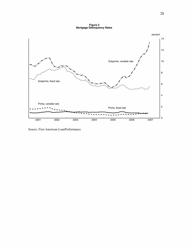
quite well, with delinquency rates trending down to historically low levels by the middle

of 2005 (figure 3). In light of the rapid home-price appreciation and overall housing

market activity (in terms of both home sales and residential construction) and the strong

performance of sumbprime mortgages through this phase, borrowers appeared to be more

willing to take on more mortgage debt and investors appeared to be more willing to fund

new mortgage originations. Consequently, underwriting standards for subprime

mortgages were loosened quite a bit and some borrowers stretched pretty far. Data show

that by 2006, many subprime variable-rate mortgages were being extended to borrowers

with less complete documentation regarding their incomes compared with originations in

earlier years, and, most importantly, with significantly higher loan-to-value ratios (LTVs)

at origination. Indeed, the share of subprime variable rate mortgages extended to

borrowers with second liens, or so-called piggyback loans, at origination appears to have

jumped late in 2005 and in 2006.

Over the past two years, the performance of subprime variable-rate mortgages has

deteriorated substantially—the delinquency rate climbed to 13½ percent in June 2007

from about half that rate in mid-2005 (figure 3). Although we certainly do not have a

complete understanding of all of the factors that contributed to the surge in delinquencies

for subprime variable-rate mortgages, it now seems very likely that at least some

borrowers and lenders had come to expect a continuation of rapid home-price

appreciation. As I already mentioned, house prices slowed appreciably in 2006,

undoubtedly leaving some subprime borrowers who had taken out very high LTV

mortgages with little or no equity to draw on should they have run into trouble with their

mortgage payments. The lack of home equity probably made it quite difficult for many

subprime borrowers to refinance their variable-rate mortgages toward the end of their

interest-rate lock period, which they may have been counting on doing. The very high

LTVs at origination also left some borrowers with an incentive to walk away from

properties that had declined in value, particularly owner-investors, whose main

attachment to these homes comes from purely financial considerations.

This spring, as you know, investors abruptly pulled back from funding subprime

mortgages, and in the past couple of months a number of large financial institutions

announced substantial changes to their subprime variable-rate mortgage programs. These

28

Source. First American LoanPerformance

Figure 3Mortgage Delinquency Rates

2001 2002 2003 2004 2005 2006 20070

2

4

6

8

10

12

14

0

2

4

6

8

10

12

14

percent

Subprime, variable rate

Subprime, fixed rate

Prime, variable rate

Prime, fixed rate

29

developments have resulted in this form of lending being sharply curtailed. In addition,

recent indications suggest that investors also seem to have become less willing to buy

securities backed by so-called Alt-A mortgage pools—pools of loans to borrowers who

typically have higher credit scores than subprime borrowers but whose applications may

contain other risky aspects. As a result of the deterioration in investor sentiment for these

types of loans, it has reportedly become much more difficult for some borrowers to

qualify for them or at least much more expensive for them to obtain.

The loosening of mortgage underwriting practices along with the unrealistic

expectations for house prices probably boosted housing demand in 2005 and 2006 and

the evident sharp reduction in nontraditional mortgage lending this year is, no doubt,

contributing importantly to the extent and persistence of the weakness in the housing

market. Moreover, as investors pulled back this summer from funding nontraditional

mortgages, spreads on corporate bonds and credit derivatives widened and measures of

implied volatility increased significantly, which signaled market participants’ greater

uncertainty about prospects. Corporate bond issuance has slowed appreciably from the

spring’s rapid pace and, in recent weeks, liquidity in the asset-backed commercial paper

market has deteriorated. These developments led the Federal Open Market Committee to

announce in mid-August that in its view the downside risks to economic growth had

increased appreciably.

As these events illustrate, under certain conditions the housing sector can be a

source of financial instability. But this leads to the second question I posed at the start of

this section: Does financial instability necessarily alter the functioning of the monetary

transmission mechanism in a marked way? One can conceive of cases in which financial

instability could seriously limit the normal functioning of the monetary transmission

mechanism, but in my view these should be rare. Barring cases in which the zero bound

on nominal policy rates is a constraint, as it was in Japan, the modern era contains few, if

any, clear examples of a breakdown in the monetary transmission mechanism.

30

III. Policy Issues

The discussion of the role of housing in the monetary transmission mechanism

raises two key policy issues: (1) How can monetary policy makers deal with the

uncertainty with regard to housing-related monetary transmission mechanisms? (2) How

can monetary policy best respond to fluctuations in asset prices, especially house prices,

and to possible asset-price bubbles?

Uncertainty Around Housing-Related Monetary Transmission Mechanisms

In recent years, we have learned a lot about housing-related monetary

transmission mechanisms. However, as our tour of these mechanisms indicates, the

importance of particular transmission mechanisms is still highly uncertain. First, we do

not have a full understanding of the dynamics of residential construction. Econometric

models of residential construction activity still leave a great deal to be desired. In the

current cycle, the various models used by the Federal Reserve Board’s staff to analyze

housing market developments generally cannot account for the full extent of the boom

and bust in residential construction.21

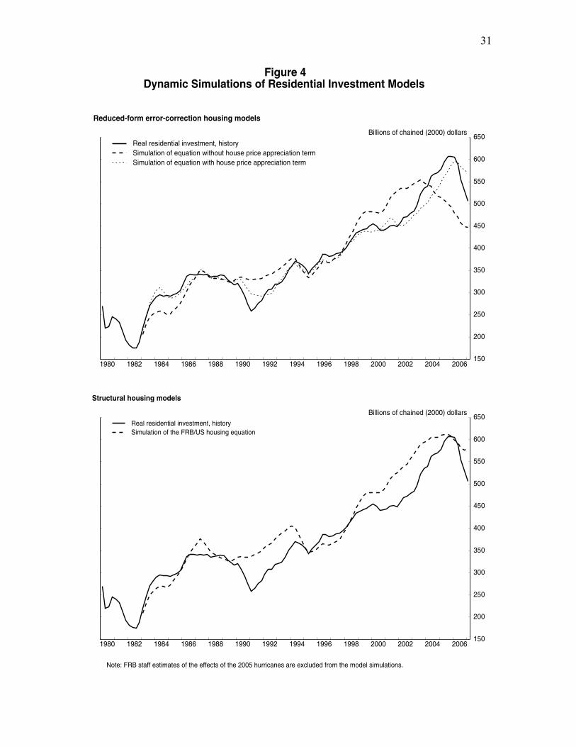
Figure 4 documents this limited ability to explain recent developments. The top

panel shows results from dynamic simulations of two reduced-form error-correction

models monitored by the Board’s staff. The first of these equations (shown as the dashed

line) relates the long-run desired level of real investment spending to fundamentals such

as income and the cost of capital for housing; the latter variable does not factor in any

effects of expected increases in real home prices. The second model (shown as the dotted

line) allows for an estimated contribution to current construction activity from the recent

lagged trend in real home-price appreciation. In both cases, the two simulations are

conditioned on the actual paths of real income, interest rates, and other factors as they

evolved after 1983. As can be seen, the standard model does a poor job of tracking the

21 General descriptions of the FRB/US model can be found in Brayton and Tinsley (1996); Brayton, Levin, and others (1997); Brayton, Mauskopf, and others (1997): and Reifschneider, Tetlow, and Williams (1999).

31

Figure 4Dynamic Simulations of Residential Investment Models

1980 1982 1984 1986 1988 1990 1992 1994 1996 1998 2000 2002 2004 2006150

200

250

300

350

400

450

500

550

600

650

150

200

250

300

350

400

450

500

550

600

650 Billions of chained (2000) dollars

Real residential investment, historySimulation of equation without house price appreciation termSimulation of equation with house price appreciation term

Reduced-form error-correction housing models

1980 1982 1984 1986 1988 1990 1992 1994 1996 1998 2000 2002 2004 2006150

200

250

300

350

400

450

500

550

600

650

150

200

250

300

350

400

450

500

550

600

650 Billions of chained (2000) dollars

Real residential investment, historySimulation of the FRB/US housing equation

Structural housing models

Note: FRB staff estimates of the effects of the 2005 hurricanes are excluded from the model simulations.

32

recent boom-and-bust cycle; the expected-capital-gains model does only somewhat

better. As shown in the bottom panel of figure 4, dynamic simulations of the structural

housing equation in the FRB/US model show a similar limited ability to track the

movements in residential construction since the mid-1990s.

Also, as discussed earlier, we are not at all sure what role expected house-price

appreciation should play in the user cost of capital. Does expected house-price

appreciation that includes the appreciation of land values belong in the user-cost measure,

or should appreciation in land values be stripped out? The issue is being explored at the

Board.

Second, as the previous discussion of the housing-wealth transmission mechanism

made clear, the size of the effect of housing wealth on consumer spending is subject to a

very wide range of estimates. This uncertainty is likely to grow in the future because

financial innovation is producing major institutional changes in mortgage markets

throughout the world, innovations that are likely to affect the sensitivity of consumer

spending to housing wealth.

Third, we do not have a firm understanding of what determines house prices and

how they respond to changes in interest rates. Furthermore, we are not even sure if

observed house prices are consistent with underlying fundamentals.22 Indeed, as noted at

the outset of this section, the question of whether house prices are currently overvalued is

the subject of active debate. For example, Shiller (2005) argues that the recent run-up in

house prices is unprecedented in the United States and represents an asset-price bubble.

The opposite view is taken by McCarthy and Peach (2004) and Himmelberg, Mayer, and

Sinai (2005), who argue that home valuations are mostly in line with fundamentals and

22 Finding a strong empirical link between house price fluctuations and fundamentals often proves to be difficult. Gallin (2003), for example, does not find empirical support for the hypothesis that income and house prices are cointegrated, while Campbell and others (2006) show that rent-price ratios exhibit considerable fluctuations unrelated to expected future interest rates and rents. Some research also finds that house prices are often influenced by irrational impulses. Genesove and Mayer (2001) show that sellers exhibit loss aversion, while Brunnermeier and Julliard (forthcoming) find evidence that house prices are influenced by the type of money illusion originally described by Modigliani and Cohn (1979). Other research, however, is more supportive of the view that housing-price behavior can be rationalized through traditional supply-demand channels. Glaeser, Gyourko, and Saks (2005a,b) show that house prices have risen more rapidly in communities with tight land-use restrictions, while Gallin (2004) finds that house prices and rents do respond to the level of the rent-price ratio.

33

are well explained by a combination of low long-term interest rates and strong income

growth.

Uncertainty about housing-related monetary transmission argues for humility on

the part of monetary policy makers regarding our understanding of the monetary

transmission mechanism generally and the appropriate settings of monetary policy

instruments. The uncertainty also suggests that policymakers keep an open mind about

specific transmission mechanisms because future research may change their views.

The bottom line is that blindly following the prescriptions in macroeconometric

models that embed specific monetary transmission mechanisms is a dangerous strategy

for monetary policy makers—judgment is still a necessary element of our decisions. The

uncertainty around housing-related monetary transmission mechanisms provides one

further reason why monetary policy will continue to be an art, albeit one that makes use

of science.

Monetary Policy Response to House Prices

The concern that recent run-ups in house prices may not reflect fundamentals has

led to an active debate among monetary policy makers around the world on the

appropriate reaction to fluctuations in house prices. Should central banks raise interest

rates to slow down house-price appreciation? How should central banks prepare

themselves to react if house prices decline?

We have already outlined several monetary transmission mechanisms that

indicate that house prices have important effects on aggregate demand. Because central

banks are in the business of managing the level of aggregate demand in the economy to

produce desirable outcomes for both inflation and employment, it makes sense for them

to respond to home prices to the extent that these prices are affecting aggregate demand

and resource utilization.

To illustrate what might be an appropriate response to a house-price decline, we

can again turn to simulations with the Federal Reserve Board’s FRB/US model. Figure 5

shows the effect of a 20 percent decline in house prices spread evenly over the two-year

period from 2007 to 2008. A 20 percent decline would be very large by U.S. standards;

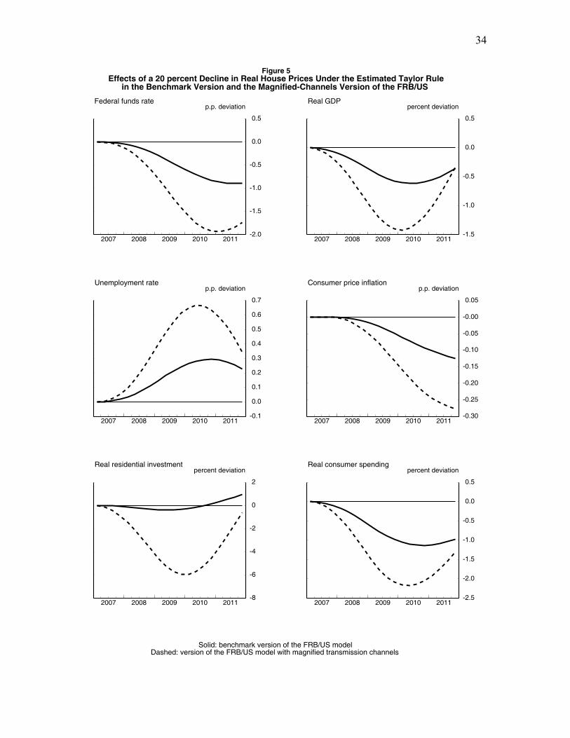
34

Figure 5Effects of a 20 percent Decline in Real House Prices Under the Estimated Taylor Rule

in the Benchmark Version and the Magnified-Channels Version of the FRB/US

Solid: benchmark version of the FRB/US modelDashed: version of the FRB/US model with magnified transmission channels

2007 2008 2009 2010 2011-2.0

-1.5

-1.0

-0.5

0.0

0.5

-2.0

-1.5

-1.0

-0.5

0.0

0.5

p.p. deviation

Federal funds rate

2007 2008 2009 2010 2011-1.5

-1.0

-0.5

0.0

0.5

-1.5

-1.0

-0.5

0.0

0.5

percent deviation

Real GDP

2007 2008 2009 2010 2011-0.1

0.0

0.1

0.2

0.3

0.4

0.5

0.6

0.7

-0.1

0.0

0.1

0.2

0.3

0.4

0.5

0.6

0.7

p.p. deviation

Unemployment rate

2007 2008 2009 2010 2011-0.30

-0.25

-0.20

-0.15

-0.10

-0.05

-0.00

0.05

-0.30

-0.25

-0.20

-0.15

-0.10

-0.05

-0.00

0.05

p.p. deviation

Consumer price inflation

2007 2008 2009 2010 2011-8

-6

-4

-2

0

2

-8

-6

-4

-2

0

2

percent deviation

Real residential investment

2007 2008 2009 2010 2011-2.5

-2.0

-1.5

-1.0

-0.5

0.0

0.5

-2.5

-2.0

-1.5

-1.0

-0.5

0.0

0.5

percent deviation

Real consumer spending

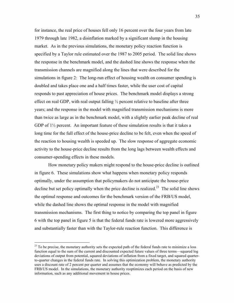
35

for instance, the real price of houses fell only 16 percent over the four years from late

1979 through late 1982, a disinflation marked by a significant slump in the housing

market. As in the previous simulations, the monetary policy reaction function is

specified by a Taylor rule estimated over the 1987 to 2005 period. The solid line shows

the response in the benchmark model, and the dashed line shows the response when the

transmission channels are magnified along the lines that were described for the

simulations in figure 2: The long-run effect of housing wealth on consumer spending is

doubled and takes place one and a half times faster, while the user cost of capital

responds to past appreciation of house prices. The benchmark model displays a strong

effect on real GDP, with real output falling ½ percent relative to baseline after three

years; and the response in the model with magnified transmission mechanisms is more

than twice as large as in the benchmark model, with a slightly earlier peak decline of real

GDP of 1½ percent. An important feature of these simulation results is that it takes a

long time for the full effect of the house-price decline to be felt, even when the speed of

the reaction to housing wealth is speeded up. The slow response of aggregate economic

activity to the house-price decline results from the long lags between wealth effects and

consumer-spending effects in these models.

How monetary policy makers might respond to the house-price decline is outlined

in figure 6. These simulations show what happens when monetary policy responds

optimally, under the assumption that policymakers do not anticipate the house-price

decline but set policy optimally when the price decline is realized.23 The solid line shows

the optimal response and outcomes for the benchmark version of the FRB/US model,

while the dashed line shows the optimal response in the model with magnified

transmission mechanisms. The first thing to notice by comparing the top panel in figure

6 with the top panel in figure 5 is that the federal funds rate is lowered more aggressively

and substantially faster than with the Taylor-rule reaction function. This difference is

23 To be precise, the monetary authority sets the expected path of the federal funds rate to minimize a loss function equal to the sum of the current and discounted expected future values of three terms—squared log deviations of output from potential, squared deviations of inflation from a fixed target, and squared quarter-to-quarter changes in the federal funds rate. In solving this optimization problem, the monetary authority uses a discount rate of 2 percent per quarter and assumes that the economy will behave as predicted by the FRB/US model. In the simulations, the monetary authority reoptimizes each period on the basis of new information, such as any additional movement in house prices.

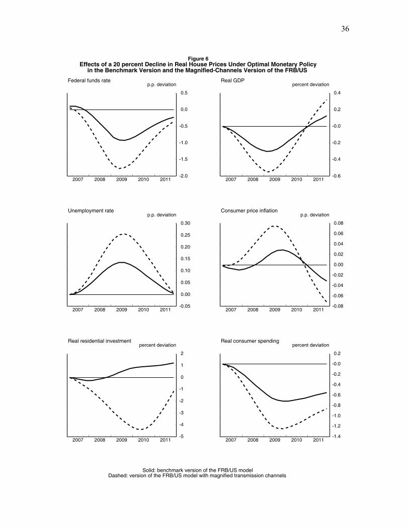
36

Figure 6Effects of a 20 percent Decline in Real House Prices Under Optimal Monetary Policy

in the Benchmark Version and the Magnified-Channels Version of the FRB/US

Solid: benchmark version of the FRB/US modelDashed: version of the FRB/US model with magnified transmission channels

2007 2008 2009 2010 2011-2.0

-1.5

-1.0

-0.5

0.0

0.5

-2.0

-1.5

-1.0

-0.5

0.0

0.5

p.p. deviation

Federal funds rate

2007 2008 2009 2010 2011-0.6

-0.4

-0.2

-0.0

0.2

0.4

-0.6

-0.4

-0.2

-0.0

0.2

0.4

percent deviation

Real GDP

2007 2008 2009 2010 2011-0.05

0.00

0.05

0.10

0.15

0.20

0.25

0.30

-0.05

0.00

0.05

0.10

0.15

0.20

0.25

0.30

p.p. deviation

Unemployment rate

2007 2008 2009 2010 2011-0.08

-0.06

-0.04

-0.02

0.00

0.02

0.04

0.06

0.08

-0.08

-0.06

-0.04

-0.02

0.00

0.02

0.04

0.06

0.08

p.p. deviation

Consumer price inflation

2007 2008 2009 2010 2011-5

-4

-3

-2

-1

0

1

2

-5

-4

-3

-2

-1

0

1

2

percent deviation

Real residential investment

2007 2008 2009 2010 2011-1.4

-1.2

-1.0

-0.8

-0.6

-0.4

-0.2

-0.0

0.2

-1.4

-1.2

-1.0

-0.8

-0.6

-0.4

-0.2

-0.0

0.2

percent deviation

Real consumer spending

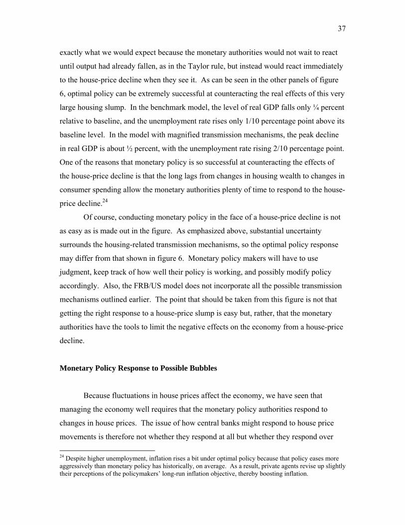
37

exactly what we would expect because the monetary authorities would not wait to react

until output had already fallen, as in the Taylor rule, but instead would react immediately

to the house-price decline when they see it. As can be seen in the other panels of figure

6, optimal policy can be extremely successful at counteracting the real effects of this very

large housing slump. In the benchmark model, the level of real GDP falls only ¼ percent

relative to baseline, and the unemployment rate rises only 1/10 percentage point above its

baseline level. In the model with magnified transmission mechanisms, the peak decline

in real GDP is about ½ percent, with the unemployment rate rising 2/10 percentage point.

One of the reasons that monetary policy is so successful at counteracting the effects of

the house-price decline is that the long lags from changes in housing wealth to changes in

consumer spending allow the monetary authorities plenty of time to respond to the house-

price decline.24

Of course, conducting monetary policy in the face of a house-price decline is not

as easy as is made out in the figure. As emphasized above, substantial uncertainty

surrounds the housing-related transmission mechanisms, so the optimal policy response

may differ from that shown in figure 6. Monetary policy makers will have to use

judgment, keep track of how well their policy is working, and possibly modify policy

accordingly. Also, the FRB/US model does not incorporate all the possible transmission

mechanisms outlined earlier. The point that should be taken from this figure is not that

getting the right response to a house-price slump is easy but, rather, that the monetary

authorities have the tools to limit the negative effects on the economy from a house-price

decline.

Monetary Policy Response to Possible Bubbles

Because fluctuations in house prices affect the economy, we have seen that

managing the economy well requires that the monetary policy authorities respond to

changes in house prices. The issue of how central banks might respond to house price

movements is therefore not whether they respond at all but whether they respond over

24 Despite higher unemployment, inflation rises a bit under optimal policy because that policy eases more aggressively than monetary policy has historically, on average. As a result, private agents revise up slightly their perceptions of the policymakers’ long-run inflation objective, thereby boosting inflation.

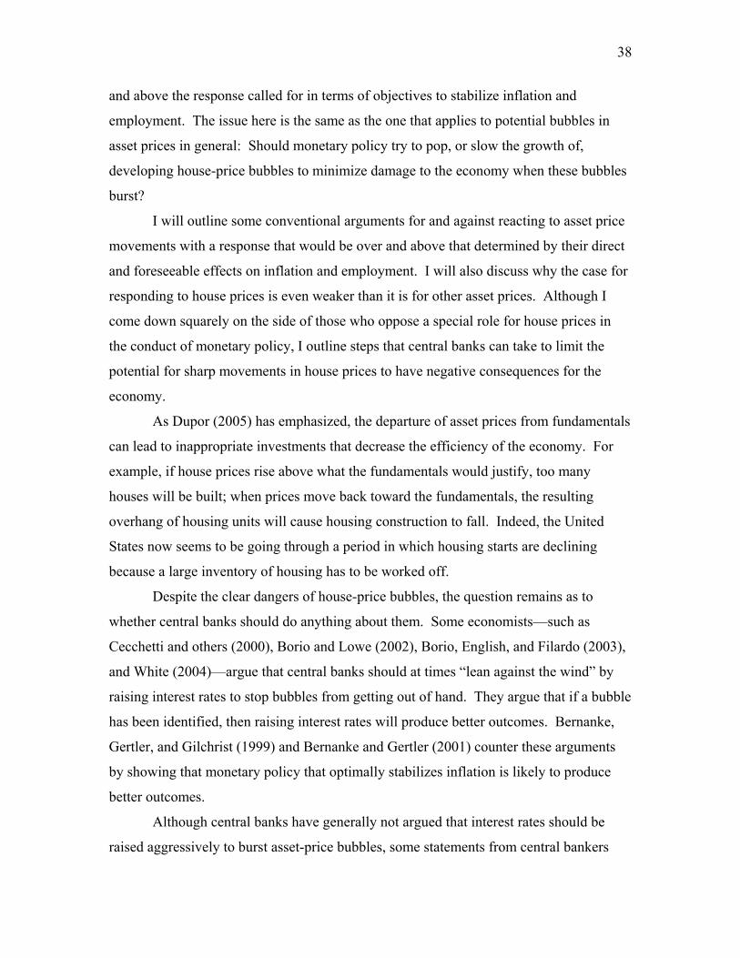
38

and above the response called for in terms of objectives to stabilize inflation and

employment. The issue here is the same as the one that applies to potential bubbles in

asset prices in general: Should monetary policy try to pop, or slow the growth of,

developing house-price bubbles to minimize damage to the economy when these bubbles

burst?

I will outline some conventional arguments for and against reacting to asset price

movements with a response that would be over and above that determined by their direct

and foreseeable effects on inflation and employment. I will also discuss why the case for

responding to house prices is even weaker than it is for other asset prices. Although I

come down squarely on the side of those who oppose a special role for house prices in

the conduct of monetary policy, I outline steps that central banks can take to limit the

potential for sharp movements in house prices to have negative consequences for the

economy.

As Dupor (2005) has emphasized, the departure of asset prices from fundamentals

can lead to inappropriate investments that decrease the efficiency of the economy. For

example, if house prices rise above what the fundamentals would justify, too many

houses will be built; when prices move back toward the fundamentals, the resulting

overhang of housing units will cause housing construction to fall. Indeed, the United

States now seems to be going through a period in which housing starts are declining

because a large inventory of housing has to be worked off.

Despite the clear dangers of house-price bubbles, the question remains as to

whether central banks should do anything about them. Some economists—such as

Cecchetti and others (2000), Borio and Lowe (2002), Borio, English, and Filardo (2003),

and White (2004)—argue that central banks should at times “lean against the wind” by

raising interest rates to stop bubbles from getting out of hand. They argue that if a bubble

has been identified, then raising interest rates will produce better outcomes. Bernanke,

Gertler, and Gilchrist (1999) and Bernanke and Gertler (2001) counter these arguments

by showing that monetary policy that optimally stabilizes inflation is likely to produce

better outcomes.

Although central banks have generally not argued that interest rates should be

raised aggressively to burst asset-price bubbles, some statements from central bankers

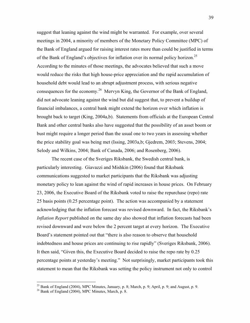
39

suggest that leaning against the wind might be warranted. For example, over several

meetings in 2004, a minority of members of the Monetary Policy Committee (MPC) of

the Bank of England argued for raising interest rates more than could be justified in terms

of the Bank of England’s objectives for inflation over its normal policy horizon.25

According to the minutes of those meetings, the advocates believed that such a move

would reduce the risks that high house-price appreciation and the rapid accumulation of

household debt would lead to an abrupt adjustment process, with serious negative

consequences for the economy.26 Mervyn King, the Governor of the Bank of England,

did not advocate leaning against the wind but did suggest that, to prevent a buildup of

financial imbalances, a central bank might extend the horizon over which inflation is

brought back to target (King, 2004a,b). Statements from officials at the European Central

Bank and other central banks also have suggested that the possibility of an asset boom or

bust might require a longer period than the usual one to two years in assessing whether

the price stability goal was being met (Issing, 2003a,b; Gjedrem, 2003; Stevens, 2004;

Selody and Wilkins, 2004; Bank of Canada, 2006; and Rosenberg, 2006).

The recent case of the Sveriges Riksbank, the Swedish central bank, is

particularly interesting. Giavazzi and Mishkin (2006) found that Riksbank

communications suggested to market participants that the Riksbank was adjusting

monetary policy to lean against the wind of rapid increases in house prices. On February

23, 2006, the Executive Board of the Riksbank voted to raise the repurchase (repo) rate

25 basis points (0.25 percentage point). The action was accompanied by a statement

acknowledging that the inflation forecast was revised downward. In fact, the Riksbank’s

Inflation Report published on the same day also showed that inflation forecasts had been

revised downward and were below the 2 percent target at every horizon. The Executive

Board’s statement pointed out that “there is also reason to observe that household

indebtedness and house prices are continuing to rise rapidly” (Sveriges Riksbank, 2006).

It then said, “Given this, the Executive Board decided to raise the repo rate by 0.25

percentage points at yesterday’s meeting.” Not surprisingly, market participants took this

statement to mean that the Riksbank was setting the policy instrument not only to control

25 Bank of England (2004), MPC Minutes, January, p. 8; March, p. 9; April, p. 9; and August, p. 9. 26 Bank of England (2004), MPC Minutes, March, p. 8.

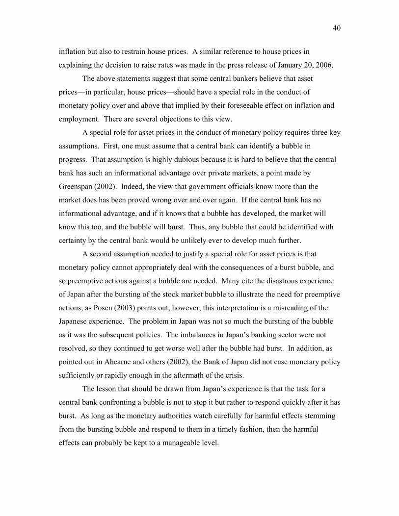
40

inflation but also to restrain house prices. A similar reference to house prices in

explaining the decision to raise rates was made in the press release of January 20, 2006.

The above statements suggest that some central bankers believe that asset

prices—in particular, house prices—should have a special role in the conduct of

monetary policy over and above that implied by their foreseeable effect on inflation and

employment. There are several objections to this view.

A special role for asset prices in the conduct of monetary policy requires three key

assumptions. First, one must assume that a central bank can identify a bubble in

progress. That assumption is highly dubious because it is hard to believe that the central

bank has such an informational advantage over private markets, a point made by

Greenspan (2002). Indeed, the view that government officials know more than the

market does has been proved wrong over and over again. If the central bank has no

informational advantage, and if it knows that a bubble has developed, the market will

know this too, and the bubble will burst. Thus, any bubble that could be identified with

certainty by the central bank would be unlikely ever to develop much further.

A second assumption needed to justify a special role for asset prices is that

monetary policy cannot appropriately deal with the consequences of a burst bubble, and

so preemptive actions against a bubble are needed. Many cite the disastrous experience

of Japan after the bursting of the stock market bubble to illustrate the need for preemptive

actions; as Posen (2003) points out, however, this interpretation is a misreading of the

Japanese experience. The problem in Japan was not so much the bursting of the bubble

as it was the subsequent policies. The imbalances in Japan’s banking sector were not

resolved, so they continued to get worse well after the bubble had burst. In addition, as

pointed out in Ahearne and others (2002), the Bank of Japan did not ease monetary policy

sufficiently or rapidly enough in the aftermath of the crisis.

The lesson that should be drawn from Japan’s experience is that the task for a

central bank confronting a bubble is not to stop it but rather to respond quickly after it has

burst. As long as the monetary authorities watch carefully for harmful effects stemming

from the bursting bubble and respond to them in a timely fashion, then the harmful

effects can probably be kept to a manageable level.

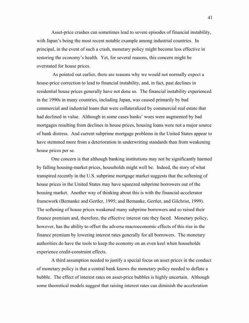
41

Asset-price crashes can sometimes lead to severe episodes of financial instability,

with Japan’s being the most recent notable example among industrial countries. In

principal, in the event of such a crash, monetary policy might become less effective in

restoring the economy’s health. Yet, for several reasons, this concern might be

overstated for house prices.

As pointed out earlier, there are reasons why we would not normally expect a

house-price correction to lead to financial instability, and, in fact, past declines in

residential house prices generally have not done so. The financial instability experienced

in the 1990s in many countries, including Japan, was caused primarily by bad

commercial and industrial loans that were collateralized by commercial real estate that

had declined in value. Although in some cases banks’ woes were augmented by bad

mortgages resulting from declines in house prices, housing loans were not a major source

of bank distress. And current subprime mortgage problems in the United States appear to

have stemmed more from a deterioration in underwriting standards than from weakening

house prices per se.

One concern is that although banking institutions may not be significantly harmed

by falling housing-market prices, households might well be. Indeed, the story of what

transpired recently in the U.S. subprime mortgage market suggests that the softening of

house prices in the United States may have squeezed subprime borrowers out of the

housing market. Another way of thinking about this is with the financial-accelerator

framework (Bernanke and Gertler, 1995; and Bernanke, Gertler, and Gilchrist, 1999).

The softening of house prices weakened many subprime borrowers and so raised their

finance premium and, therefore, the effective interest rate they faced. Monetary policy,

however, has the ability to offset the adverse macroeconomic effects of this rise in the

finance premium by lowering interest rates generally for all borrowers. The monetary

authorities do have the tools to keep the economy on an even keel when households

experience credit-constraint effects.

A third assumption needed to justify a special focus on asset prices in the conduct

of monetary policy is that a central bank knows the monetary policy needed to deflate a

bubble. The effect of interest rates on asset-price bubbles is highly uncertain. Although

some theoretical models suggest that raising interest rates can diminish the acceleration

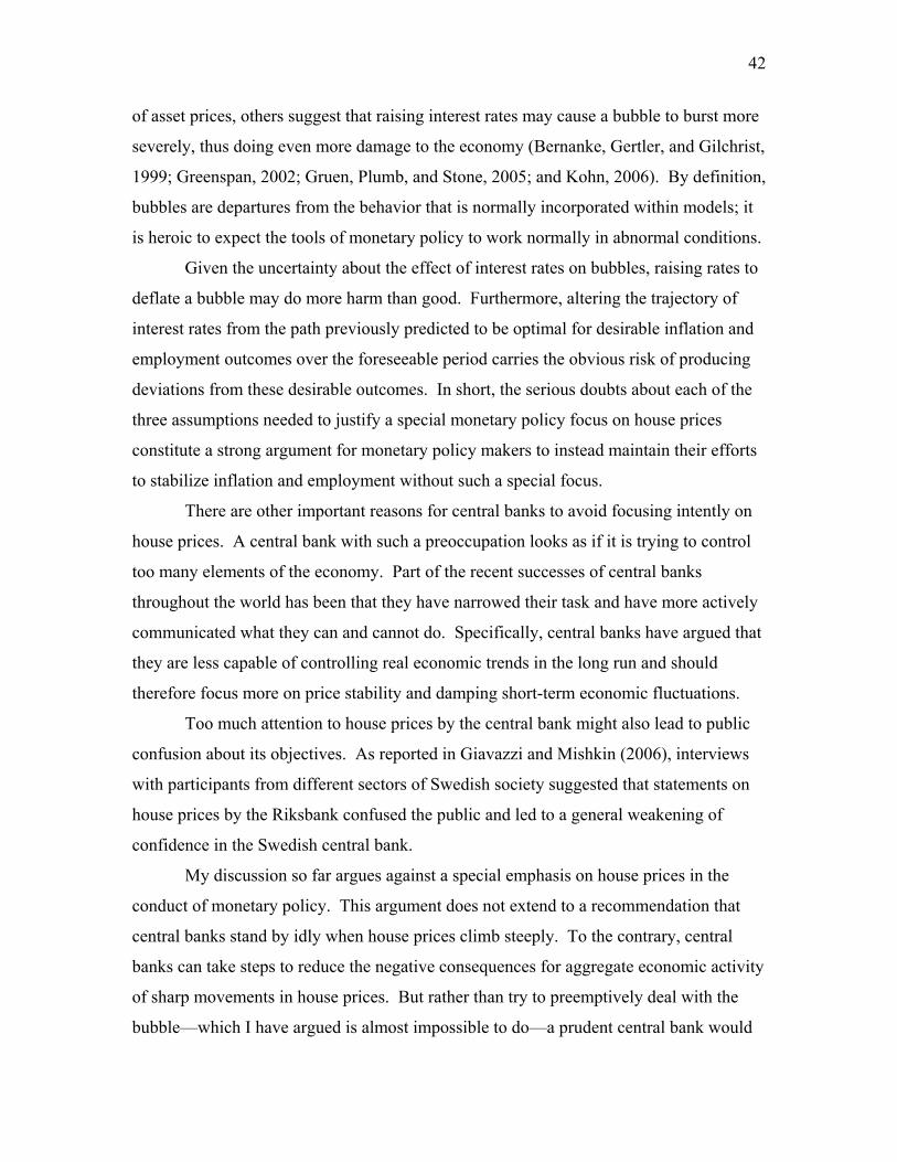
42

of asset prices, others suggest that raising interest rates may cause a bubble to burst more

severely, thus doing even more damage to the economy (Bernanke, Gertler, and Gilchrist,

1999; Greenspan, 2002; Gruen, Plumb, and Stone, 2005; and Kohn, 2006). By definition,

bubbles are departures from the behavior that is normally incorporated within models; it

is heroic to expect the tools of monetary policy to work normally in abnormal conditions.

Given the uncertainty about the effect of interest rates on bubbles, raising rates to

deflate a bubble may do more harm than good. Furthermore, altering the trajectory of

interest rates from the path previously predicted to be optimal for desirable inflation and

employment outcomes over the foreseeable period carries the obvious risk of producing

deviations from these desirable outcomes. In short, the serious doubts about each of the

three assumptions needed to justify a special monetary policy focus on house prices

constitute a strong argument for monetary policy makers to instead maintain their efforts

to stabilize inflation and employment without such a special focus.

There are other important reasons for central banks to avoid focusing intently on

house prices. A central bank with such a preoccupation looks as if it is trying to control

too many elements of the economy. Part of the recent successes of central banks

throughout the world has been that they have narrowed their task and have more actively

communicated what they can and cannot do. Specifically, central banks have argued that

they are less capable of controlling real economic trends in the long run and should

therefore focus more on price stability and damping short-term economic fluctuations.

Too much attention to house prices by the central bank might also lead to public

confusion about its objectives. As reported in Giavazzi and Mishkin (2006), interviews

with participants from different sectors of Swedish society suggested that statements on

house prices by the Riksbank confused the public and led to a general weakening of

confidence in the Swedish central bank.

My discussion so far argues against a special emphasis on house prices in the

conduct of monetary policy. This argument does not extend to a recommendation that

central banks stand by idly when house prices climb steeply. To the contrary, central

banks can take steps to reduce the negative consequences for aggregate economic activity

of sharp movements in house prices. But rather than try to preemptively deal with the

bubble—which I have argued is almost impossible to do—a prudent central bank would

43

be better advised to deal with adverse macroeconomic consequences as they emerge in

the wake of any substantial decline in asset prices. One way a central bank can prepare

itself to react quickly is to explore various scenarios as a normal part of its business to

assess how it might respond to a variety of shocks, including a drop in house prices, to

achieve maximum sustainable employment and price stability.

Indeed, the exploration of different scenarios by the central bank can be thought

of as stress testing similar to that regularly conducted by commercial financial institutions

and banking supervisors. They see how financial institutions will be affected by

particular scenarios and then propose plans to ensure that the banks can withstand the

negative effects. By conducting similar exercises, in this case for monetary policy, a

central bank can mitigate the effects of a drop in house prices without having to judge

that a bubble may be in progress or predict when a bubble might burst.

One objection to an easing of monetary policy following the collapse of an asset

bubble is that it might lead market participants to believe that the central bank will

always act to prop up asset prices, a belief that can make a bubble more likely. The

central bank can mitigate such an interpretation, however, if it publicly emphasizes that

its monetary policy is not directed at stabilizing any particular asset price but is rather

focused on achieving price stability and maximum sustainable employment. Making sure

that a house-price collapse does not do serious harm to the aggregate economy in no way

eliminates sharp declines in house prices and so does not provide insurance against such

declines. The same reasoning holds true for stock prices. Indeed, we have seen

substantial declines in housing and other asset prices in many countries even when

monetary policy has been eased substantially.

Central banks with supervisory authority can also make bubbles less likely

through prudential supervision of the financial system. If elevated house prices are

leading to excessive risk-taking on the part of financial institutions, the central bank,

along with other supervisory agencies, can encourage financial institutions to have

appropriate risk-management practices in place. Besides helping make financial

institutions better able to cope with possible house-price declines, working through

supervisory channels could also have the indirect effect of moderating house prices

should they be stimulated by excessive bank financing. Also, reminding institutions to

44

maintain risk-management practices appropriate to the economic and financial

environment could potentially help lessen a buildup of excessive house prices in the first

place.

Even if the central bank is not involved directly in prudential supervision, it can

still play a role through public communication, particularly if it has a vehicle like the

financial-stability reports that some central banks publish. In these reports, central banks

can evaluate whether increases in asset prices might be leading to excessive risk-taking

on the part of financial institutions or whether distortions from inappropriate tax or

regulatory policies may be stimulating excessive valuations of assets. If such distortions

appear to be happening, the central bank’s discussion might encourage policy adjustment

to remove the distortions or encourage prudential regulators and supervisors to more

closely monitor the financial institutions they supervise.

Large run-ups in asset prices present serious challenges to central bankers. The

analysis of the role of housing in the monetary transmission mechanism argues against a

special role for house prices in the conduct of monetary policy and in favor of a policy

response to them only to the extent that they have foreseeable effects on inflation and

employment. Nevertheless, central banks can take measures to prepare for possible sharp

reversals in the prices of homes or other assets to ensure that they will not do serious

harm to the economy.

45

REFERENCES Ahearne, Alan G., John Ammer, Brian M. Doyle, Linda S. Kole, and Robert F. Martin (2005). “House Prices and Monetary Policy: A Cross-Country Study,” International Finance Discussion Papers 841 (Washington: Board of Governors of the Federal Reserve System, September). Ahearne, Alan G., Joseph E. Gagnon, Jane Haltmaier, and Steven B. Kamin (2002). “Preventing Deflation: Lessons from Japan's Experience in the 1990s,” International Finance Discussion Papers 729 (Washington: Board of Governors of the Federal Reserve System, June). Ando, Albert, and Franco Modigliani (1963). “The ‘Life-Cycle’ Hypothesis of Saving: Aggregate Implications and Tests,” American Economic Review, vol. 53 (March), pp. 55-84. Aoki, K., James Proudman, and G. Vlieghe (2002). “House Prices, Consumption and Monetary Policy: A Financial Accelerator Approach,” Bank of England Working Paper No. 169 (London: Bank of England). Attanasio, O., L. Blow, R. Hamilton, and A. Leicester (2005). “Consumption, House Prices, and Expectations,” Bank of England Working Paper No. 271 (London: Bank of England, September). Avery, Robert B., Kenneth P. Brevoort, and Glenn B. Canner (2006). “Higher-Priced Home Lending and the 2005 HMDA Data,” Federal Reserve Bulletin, vol. 92 (September), pp. A123-66, www.federalreserve.gov/pubs/bulletin/default.htm. Bank of Canada (2006). Renewal of the Inflation-Control Target: Background Information (Ottawa: Bank of Canada), www.bank-banque-canada.ca/en/press. Bank of England (various years). Minutes of the Monetary Policy Committee, www.bankofengland.co.uk/publications/minutes/mpc. Bayoumi, Tamim, and Hali Edison (2003). “Is Wealth Increasingly Driving Consumption?” DNB Staff Reports 100 (Amsterdam: De Nederlandsche Bank). Belsky, E., and J. Prakken (2004). “Housing Wealth Effects: Housing’s Impact on Wealth Accumulation, Wealth Distribution and Consumer Spending” (Chicago: National Center for Real Estate Research). Benito, A., J. Thompson, M. Waldron, and R. Wood (2006). “House Prices and Consumer Spending,” Bank of England Quarterly Bulletin, vol. 46 (Summer), pp. 142-54.

46

Bennett, P., R. Peach, and S. Peristiani (2001). “Structural Change in the Mortgage Market and the Propensity to Refinance,” Journal of Money, Credit and Banking, vol. 33 (no. 4), pp. 955-75. Bernanke, B., and M. Gertler (1995). “Inside the Black Box: The Credit Channel of Monetary Policy Transmission,” Journal of Economic Perspectives, vol. 9 (no. 4), pp. 27-48. Bernanke, B., and M. Gertler (2001). “Should Central Banks Respond to Movements in Asset Prices?” American Economic Review, vol. 91 (no. 2), pp. 253-57. Bernanke, B., M. Gertler, and S. Gilchrist (1999). “The Financial Accelerator in a Quantitative Business Cycle Framework” in J. B. Taylor and M. Woodford, eds., Handbook of Macroeconomics (New York: Elsevier Science--North Holland), vol. 1C, pp. 1341-93. Borio, C., W.B. English, and A.J. Filardo (2003). “A Tale of Two Perspectives: Old or New Challenges for Monetary Policy?” BIS Working Paper No. 127 (Basel: Bank for International Settlements, February). Borio, Claudio, and Philip Lowe (2002). “Asset Prices, Financial and Monetary Stability: Exploring the Nexus,” BIS Working Paper 114 (Basel: Bank for International Settlements, July). Bostic, R., S. Gabriel, and G. Painter (2004). “Housing Wealth, Financial Wealth, and Consumption: New Evidence from Microdata,” USC Lusk Center for Real Estate Working Paper 2004-1005 (Los Angeles: University of Southern California). Brayton, Flint, and Eileen Mauskopf (1985). “The MPS Model of the United States Economy,” Economic Modeling, vol. 2 (July), pp. 170-292. Brayton, F., and P. Tinsley, eds. (1996). “A Guide to FRB/US: A Macroeconomic Model of the United States,” Finance and Economics Discussion Series Working Paper 1996-42 (Washington: Board of Governors of the Federal Reserve System, October). Brayton, F., A. Levin, R. Tryon, and J.C. Williams (1997). “The Evolution of Macro Models at the Federal Reserve Board,” Carnegie-Rochester Conference Series on Public Policy, vol. 47 (December), pp. 43-81. Brayton, Flint, Eileen Mauskopf, David Reifschneider, Peter Tinsley, and John Williams (1997). “The Role of Expectations in the FRB/US Macroeconomic Model,” Federal Reserve Bulletin, vol. 83 (April), 227-45. Brunnermeier, M., and C. Julliard (forthcoming). “Money Illusion and Housing Frenzies,” Review of Financial Studies.

47

Calza, A., T. Monacelli, and L. Stracca (2007). “Mortgage Markets, Collateral Constraints, and Monetary Policy: Do Institutional Factors Matter?” CFS Working Paper Series No. 2007/10 (Frankfurt: Center for Financial Studies). Campbell, Sean D., Morris A. Davis, Joshua Gallin, and Robert F. Martin (2006). “A Trend and Variance Decomposition of the Rent-Price Ratio in Housing Markets,” Finance and Economics Discussion Series No. 2006-29 (Washington: Board of Governors of the Federal Reserve System, August). Carroll, C., M. Otsuka, and J. Slacalek (2006). “How Large is the Housing Wealth Effect? A New Approach,” NBER Working Paper No. 12746 (Cambridge, Mass.: National Bureau of Economic Research, December). Case, Karl (1986). “The Market for Single-Family Homes in Boston,” Federal Reserve Bank of Boston, New England Economic Review, vol. 1986 (May/June), pp. 38-48. Case, K.E., J.M. Quigley, and R.J. Shiller (2005). “Comparing Wealth Effects: The Stock Market Versus the Housing Market,” Advances in Macroeconomics, vol. 5 (no. 1), www.bepress.com/bejm/advances/vol5/iss1/art1. Case, K.E., and R.J. Shiller (2003). “Is There a Bubble in the Housing Market?” Brookings Papers on Economic Activity, vol. 2, pp. 299-342. Catte, P., N. Girouard, R. Price, and C. Andre (2004). “Housing Markets, Wealth, and the Business Cycle,” OECD Economics Department Working Papers No. 394 (Paris: Organisation for Economic Co-operation and Development, June). Cecchetti , S., Genberg, H., Lipsky, J., and S. Wadhwani (2000). “Asset Prices and Central Bank Policy,” Geneva Reports on the World Economy No. 2 (London: Centre for Economic Policy Research, July). Davis, M., and J. Heathcote (forthcoming). “The Price and Quantity of Residential Land in the United States,” Journal of Monetary Economics. Davis, M., and M. Palumbo (forthcoming). “The Price of Residential Land in Large U.S. Cities,” Journal of Urban Economics. Debelle, Guy (2004). “Household Debt and the Macroeconomy,” BIS Quarterly Review, vol. 2004 (March), pp. 51-64. Drees, B., and C. Pazarbaşioğlu (1998). “The Nordic Banking Crises: Pitfalls in Financial Liberalization?” IMF Occasional Paper 161 (Washington: International Monetary Fund, April).

48

Dvornak, N., and M. Kohler (2003). “Housing Wealth, Stock Market Wealth and Consumption: A Panel Analysis for Australia,” RBA Research Discussion Papers No. RDP2003-07 (Sydney: Reserve Bank of Australia, July). Dupor, Bill (2005). “Stabilizing Non-fundamental Asset Price Movements under Discretion and Limited Information,” Journal of Monetary Economics, vol. 52 (May), pp. 727-47. Dynan, Karen E., Douglas W. Elmendorf, and Daniel E. Sichel (2005). “Can Financial Innovation Help to Explain the Reduced Volatility of Economic Activity?” Finance and Economics Discussion Series No. 2005-54 (Washington: Board of Governors of the Federal Reserve System, November). Dynan, Karen E., and Donald L. Kohn (2007). “The Rise in U.S. Household Indebtedness: Causes and Consequences,” prepared for the Reserve Bank of Australia Conference on “The Structure and the Resilience of the Financial System. Edge, Rochelle M., Michael T. Kiley, and Jean-Philippe Laforte (2007). “Natural Rate Measures in an Estimated DSGE Model of the U.S. Economy,” Finance and Economics Discussion Series Working Paper No. 2007-08 (Washington: Board of Governors of the Federal Reserve System, March). Estrella, Arturo (2002). “Securitization and the Efficacy of Monetary Policy,” Federal Reserve Bank of New York, Economic Policy Review, vol. 9 (May), pp. 243-55. Gallin, Joshua (2003). “The Long-run Relationship Between House Prices and Income: Evidence From Local Housing Markets,” Finance and Economics Discussion Series Working Paper No. 2003-17 (Washington: Board of Governors of the Federal Reserve System, April). Gallin, Joshua (2004). “The Long-Run Relationship between House Prices and Rents,” Finance and Economics Discussion Series No. 2004-50 (Washington: Board of Governors of the Federal Reserve System, September). Genesove, D., and C. Mayer (2001). “Loss Aversion and Seller Behavior: Evidence From the Housing Market,” Quarterly Journal of Economics, vol. 116, pp. 1233-60. Giavazzi, Francesco, and Frederic S. Mishkin (2006). An Evaluation of Swedish Monetary Policy Between 1995 and 2005 (Stockholm: Sveriges Riksdag). Girouard, N., and S. Blondal (2001). “House Prices and Economic Activity,” OECD Economics Department Working Papers No. 279 (Paris: Organisation for Economic Co-operation and Development, January).

49

Gjedrem, Svein (2003). “Financial Stability, Asset Prices, and Monetary Policy,” speech delivered at the Center for Monetary Economics, Norwegian School of Management, June 3. Glaeser, E., J. Gyourko, and R. Saks (2005a). “Why is Manhattan so Expensive? Regulation and the Rise of House Prices,” Journal of Law and Economics, vol. 48, pp. 331-70. Glaeser, E., Gyourko J., and R. Saks (2005b). “Why Have Housing Prices Gone Up?” American Economic Review, vol. 95 (May, Papers and Proceedings), pp. 329-33. Green, R.K., and S. Wachter (2005). “The American Mortgage in Historical and International Context,” Journal of Economic Perspectives, vol. 19 (no. 4), pp. 93-114. Greenspan, A. (1999). “Lessons from the Global Crises,” speech delivered before the World Bank Group and the International Monetary Fund, Washington, September 27. Greenspan, A. (2002). “Economic Volatility,” speech delivered at a symposium sponsored by the Federal Reserve Bank of Kansas City, Jackson Hole, Wyo., August 30. Greenspan, A. (2004). “Risk and Uncertainty in Monetary Policy,” speech delivered at the Meetings of the American Economic Association, San Diego, January 3. Greenspan, Alan, and James Kennedy (2005). “Estimates of Home Mortgage Originations, Repayments, and Debt on One-to-Four-Family Residences,” Finance and Economics Discussion Series No. 2005-41 (Washington: Board of Governors of the Federal Reserve System, September). Gruen, D., M. Plumb, and A. Stone (2005). “How Should Monetary Policy Respond to Asset Price Bubbles?” International Journal of Central Banking, vol. 1 (December), pp. 1-31. Hanushek, Eric, and John Quigley (1980). “What is the Price Elasticity of Housing Demand?” Review of Economics and Statistics, vol. 62, pp. 449-54. Hatzius, J. (2005). “Housing Holds the Key to Fed Policy,” Goldman Sachs Global Economics Paper No. 137 (New York: Goldman Sachs, February). Hendershott, Patric H. (1980). “Real User Costs and the Demand for Single-Family Housing,” Brookings Papers on Economic Activity, vol. 1980 (no. 2), pp. 401-52. Henderson, J. Vernon, and Yannis Ioannides (1986). “Tenure Choice and the Demand for Housing,” Economica, vol. 53, pp. 231-46.

50

Herring, R.J., and S.M. Wachter (1999). “Real Estate Booms and Banking Busts—An International Perspective,” Group of Thirty Occasional Paper 58 (Washington: Group of Thirty). Himmelberg, C., C. Mayer, and T. Sinai (2005). “Assessing High House Prices: Bubbles, Fundamentals and Misperceptions,” Journal of Economic Perspectives, vol. 19, pp. 67-92. Hurst, E., and F. Stafford (2004). “Home is Where the Equity Is: Mortgage Refinancing and Household Consumption,” Journal of Money, Credit and Banking, vol. 36 (no. 6), pp. 985-1014. International Monetary Fund (2004). “Three Current Policy Issues,” World Economic Outlook, Chapter II (Washington: International Monetary Fund, September), www.imf.org/external/pubs/ft/weo. International Monetary Fund (2006). “How Do Financial Systems Affect Economic Cycles,” World Economic Outlook, Chapter IV (Washington: International Monetary Fund, September), www.imf.org/external/pubs/ft/weo. Issing, Otmar (2003a). “Monetary and Financial Stability: Is There a Trade-off?” comments at the Bank for International Settlements, March. Issing, Otmar (2003b). Introductory statement delivered at the European Central Bank Workshop on “Asset Prices and Monetary Policy,” December 11. Jorgenson, Dale (1963). “Capital Theory and Investment Behavior,” American Economic Review, vol. 53 (May), pp. 247-59. Kane, Edward (1989). The S&L Insurance Mess: How Did it Happen? (Washington: Urban Institute Press). Katz, Lawrence, and Kenneth Rosen (1987). “The Interjurisdictional Effects of Growth Controls on House Prices,” Journal of Law & Economics, vol. 30, pp. 149-60. Kearl, J.R. (1979). “Inflation, Mortgages and Housing,” Journal of Political Economy, vol. 87 (no. 5), pp. 1115-38. Kearl, James R., and Frederic S. Mishkin (1977). “Illiquidity, the Demand for Residential Housing, and Monetary Policy” (with J. R. Kearl), Journal of Finance, vol. 37 (December), pp. 1571-86. King, Mervyn (2004a). Remarks made in a panel discussion on Alan Greenspan's speech on Risk and Uncertainty in Monetary Policy delivered at the American Economic Association Annual Meeting in San Diego, January 3, www.bankofengland.co.uk/publications/speeches/2004/speech209.pdf.

51

King, Mervyn (2004b). Speech delivered to the CBI Scotland Diner at the Glasgow Hilton Hotel, June 14, www.bankofengland.co.uk/publications/speeches/2004/speech221.pdf. Klyuev, V., and P. Mills (2006). “Is Housing Wealth an ATM? The Relationship Between Household Wealth, Home Equity Withdrawal, and Saving Rates,” IMF Working Paper WP/06/162 (Washington: International Monetary Fund). Kohn, Donald (2006). “Monetary Policy and Asset Prices,” speech delivered at “Monetary Policy: A Journey from Theory to Practice,” a European Central Bank Colloquium held in honor of Otmar Issing, Frankfurt, March 16. Lusardi, Annamaria (1996). “Current Income, Permanent Income, and Consumption: Evidence from Two Panel Data Sets,” Journal of Business and Economic Statistics, vol. 14 (no. 1), pp. 81-90. Ludwig, A., and T. Slok (2002). “The Impact of Changes in Stock Prices and House Prices on Consumption in OECD Countries,” IMF Working Paper No. 2002-1 (Washington: International Monetary Fund). Malpezzi, Stephen (1996). “Housing Prices, Externalities, and Regulation in U.S. Metropolitan Areas,” Journal of Housing Research, vol. 7, pp. 209-41. Mayer, C.J., and C.T. Somerville (2000). “Land Use Regulation and New Construction,” Regional Science and Urban Economics, vol. 30 (no. 6), pp. 659-83. McCarthy, J., and R. Peach (2002). “Monetary Policy Transmission to Residential Investment,” Federal Reserve Bank of New York, Economic Policy Review, vol. 8 (no. 1), pp. 139-58. McCarthy, J., and R. Peach (2004). “Are Home Prices the Next ‘Bubble’?” Federal Reserve Bank of New York, Economic Policy Review, vol. 10, pp. 1-17. Mishkin, Frederic S. (1997). “The Causes and Propagation of Financial Instability: Lessons for Policymakers,” in Maintaining Financial Stability in a Global Economy, Symposium Proceedings (Kansas City: Federal Reserve Bank of Kansas City), pp. 55-96. Mishkin, Frederic S. (2007). The Economics of Money, Banking and Financial Markets, 8th ed. (Boston: Addison Wesley). Mishkin, Frederic S., and Eugene White (2003). "U.S. Stock Market Crashes and

Their Aftermath: Implications for Monetary Policy," in William Curt Hunter, George G. Kaufman, and Michael Pormerleano, eds., Asset Price Bubbles: The Implications for Monetary, Regulatory, and International Policies (Cambridge, Mass.: MIT Press), pp.

52

53-79. Modigliani, F., and R. Brumberg (1954). “Utility Analysis and the Consumption Function: An Interpretation of Cross-Section Data,” in K. Kurihara, ed., Post Keynesian Economics (New Brunswick, N.J.: Rutgers University Press), pp. 388-436. Modigliani, F., and R.A. Cohn (1979). “Inflation, Rational Valuation and the Market,” Financial Analysts Journal, vol. 35 (March/April), pp. 24-44. Peach, Richard (1983). “An Econometric Model of Investment in Single-family Housing,” Ph.D. dissertation, University of Maryland. Poole, William (1972). “Housing Finance Under Inflationary Conditions,” in Ways to Moderate Fluctuations in Housing Construction, Federal Reserve Staff Study (Washington: Board of Governors of the Federal Reserve System). Posen, Adam S. (2003). “It Takes More Than a Bubble to Become Japan,” Reserve Bank of Australia Annual Conference, Asset Prices and Monetary Policy (Sydney: Reserve Bank of Australia), pp. 203-49. Poterba, J. (1984) “Tax Subsidies to Owner-Occupied Housing: An Asset-Market Approach,” Quarterly Journal of Economics, vol. 99 (November), pp. 729-75. Reifschneider, David, Robert Tetlow, and John Williams (1999). “Aggregate Disturbances, Monetary Policy, and the Macroeconomy: The FRB/US Perspective,” Federal Reserve Bulletin, vol. 85 (January), pp. 1-19. Robertson, R. (2006). “Thinking About the Big Drop in Australian Housing Affordability” (Sydney: Macquarie Bank, December). Rosenberg, Irma (2006). “Monetary Policy in Sweden,” speech delivered at the Swedibank, September 18. Schwab, Robert M. (1982). “Inflation Expectations and the Demand for Housing,” American Economic Review, vol. 72 (no. 1), pp. 143-53. Selody, Jack, and Carolyn Wilkins (2004). “Asset Prices and Monetary Policy: A Canadian Perspective on the Issues,” Bank of Canada Review (Autumn), pp. 3-14. Shiller, R. (2005). Irrational Exuberance, 2nd ed. (Princeton: Princeton University Press).

53

Souleles, N. (1999). “The Response of Household Consumption to Income Tax Refunds,” American Economic Review, vol. 89 (no. 4), pp. 947-58. Stevens, G.R. (2004). “Recent Issues in the Conduct of Monetary Policy,” Reserve Bank of Australia Bulletin, vol. 2004 (March). Tsatsaronis, K., and H. Zhu (2004). “What Drives House Price Dynamics: Cross-Country Evidence,” BIS Quarterly Review (March), pp. 65-78. White, William (2004). “Making Macroprudential Concerns Operational,” speech delivered at a Financial Stability Symposium organized by the Netherlands Bank, Amsterdam, October 26, www.bis.org/speeches/sp041026.htm.