Finance 590 Enterprise Risk Management Portfolio Management Mark Vonnahme.
70
Finance 590 Enterprise Risk Management Portfolio Management Mark Vonnahme
-
Upload
jonas-ward -
Category
Documents
-
view
217 -
download
3
Transcript of Finance 590 Enterprise Risk Management Portfolio Management Mark Vonnahme.
Finance 590
Enterprise Risk Management
Portfolio Management
Mark Vonnahme
ERM
• Portfolio Management– Concepts of Active Portfolio Management
provide a structure for Enterprise Risk Management
– Act like a “ Fund Manager ”• Set portfolio targets• Set risk limits• Diversification• Optimal returns
ERM
• Portfolio Management– Can these disciplines be applied to the
enterprise in managing an organization’s risks
ERM
• Portfolio Management– Theory of Active Portfolio Management
• Harry Markowitz
• Fundamental concepts– Risk
– Reward
– Diversification
– Leverage
– Hedging
ERM
• Risk– Typically equated with volatility, measure of
associated with future events– Risk indeterminate – Can estimate likely future value of investments
and some range of variation around the value
ERM
• Reward– Gain on investment is indeterminate– Can provide an estimate of expected value– Reward should be commensurate with risk
• Higher return for higher risk
• Not always the case
ERM
• Diversification– Concept of lowering risk by spreading risk
among many distinct investments, projects or opportunities
– The more dissimilar or the less the correlation between investments, the greater the diversification
– Diversification then reduces portfolio risks significantly when combined

ERM
• Leverage– Effect of borrowing to increase the risk profile
of a venture• Multiplies the risk / reward profile
ERM
• Hedging– Offsetting risk by entering a market position
negatively correlated to existing position– Motivated by desire to reduce risk of an
existing position, not a new investment• More like insurance in this position

ERM
• Portfolio Management supports ERM by– Unbundling risk origination, retention and
transfer– Providing a risk aggregation function across the
company– Setting risk limits and asset allocation targets– Influencing transfer pricing,capital allocation,
and investment decisions
ERM
• Unbundling– Manage business…core competencies and
risk /reward economics– Still must manage the business risks or
components• Where are our strengths
• What is our specialization
• Where can we be successful
ERM
• Risk Aggregation– Overall risk profile and portfolio represents
aggregation of all types of risk activities– Every company looks at it a little different
• Some thoughts

ERM
• Risk Limits and Asset Allocation– Balance between diversification and
performance• Establish risk concentration limits and allocation
targets• Limits ensure proper diversification
– Business can set similar portfolio risk limits and allocation targets
• Some personal experiences
ERM
• Influencing Transfer Pricing , Capital Allocation, and Investment Decisions– Management influences risk profile of business
portfolio in many ways• Global business provides opportunities
• Allocation of capital to businesses and products with potential for risk adjusted higher returns
– Also driven by diversification goals
ERM
• Practical Applications– Reinsurance– Currency Hedging
ERM
• Reinsurance– Case discussion from text
• Catastrophe risk
– Personal experiences• Why did we purchase reinsurance
ERM
• Currency Hedging– Our global businesses have made this a
common issue for analysis and management action
• Discussion

ERM
• Questions
• Discussion
Enterprise Risk Management
Stakeholder Management
Mark C. Vonnahme

ERM
• Who are the stakeholders– Limited view– Broad view
• Any group that supports and supports the survival and success of the company
ERM
• Stakeholders– Employees
– Customers
– Suppliers
– Business partners
– Investors
– Analysts
– Board of directors
– Regulators
ERM
• Stakeholders– Have discussed some groups already– Will concentrate on
• Employees
• Customers
• Business partners
ERM
• Employees– Changing “contract” and relationship between
employer and employees– People are still most important and demanding
asset• Management today faces a different set of
challenges

ERM
• Employment is a series of stages with a set of challenges at each– Recruiting and screening– Training and development– Retention and promotion– Firing and resignation
ERM
• Customers– For virtually all business it is most important to
success• Customer management is key strategy for success
– Attrition and acquisition
– Loyalty and a satisfaction
– Knowing the customer
– Handling crisis
ERM
• Customer management – Personal experiences
• The good , the bad, the ugly
ERM
• Business partners– The day to day– Special situations …strategic alliances
ERM
• Business partners everyday– Insurance and surety agents and brokers
• Both customer and partner
– Reinsurers– Other companies
• Working together on key risks
• Associations
ERM
• Strategic Alliances– There are pitfalls– Risk management approach
• Pros and cons
• The right partner
• Monitor progress
ERM
• Strategic Alliances– My experiences
• International opportunities– Needed partners and found them
• Customer joint ventures– Some work ; many do not
• Some “dos and don’t s”

ERM
• Summary– Stakeholder Management requires cooperation
throughout an organization

Finance 590Enterprise Risk Management
Steve D’ArcyDepartment of Finance
Lecture 4
Financial Risk Analytics
April 12, 2005

Reference Material• Chapter 13 – Market Risk Management in
Enterprise Risk Management by James Lam
• Value-at-Risk readings by Jorion http://www.gsm.uci.edu/~jorion/oc/case3.html
http://www.gsm.uci.edu/~jorion/oc/case4.html
http://www.gsm.uci.edu/~jorion/oc/case5.html
Overview
• Types of Market Risk
• Market Risk Measurement– Interest Rate Sensitivity– Value-at-Risk
Types of Market Risk
• Interest rate risk
• Foreign exchange risk
• Commodity risk
• Equity risk
• Basis risk
• Other market driven risk– Option risk– Real estate risk

Measuring Interest Rate Sensitivity
• Gap analysis
• Duration
• Convexity
• Term structure models
Duration
• First order approximation of the sensitivity of a financial instrument (asset or liability) to interest rate changes

Price/Yield Relationship
• Recall that bond prices move inversely with interest rates– As interest rates
increase, present value of fixed cash flows decrease
• For option-free bonds, this curve is not linear but convex
Price/yield curve
Yield
Pri
ce
Simplifications
• Fixed income, non-callable bonds
• Flat yield curve
• Parallel shifts in the yield curve

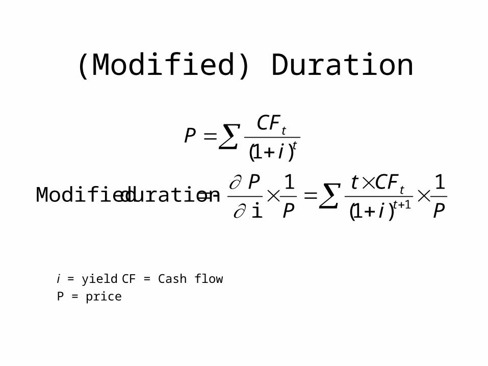
(Modified) Duration• A measure of price sensitivity is determined by
the slope of the price/yield curve
• Divide the slope by the current price to get a duration measure called modified duration
(Modified) Duration
Pi
CFt
P
P
i
CFP
tt
tt
1
)1(
1
i
duration Modified
)1(
1
i = yield CF = Cash flow
P = price

Error in Price Predictions
• The estimate of the change in bond price is at one point– The estimate is linear
• If the price/ yield curve is convex, it lies above the tangent line
• Our estimate of price is always understated Yield
Pri
ce

Convexity• The duration estimate of percentage changes in
price is a first order approximation
• If the change in interest rates is very large, our price estimate has a larger error– Duration is only accurate for small changes in interest
rates
• Convexity provides a second order approximation of the bond’s sensitivity to changes in the interest rate– Captures the curvature in the price/yield curve
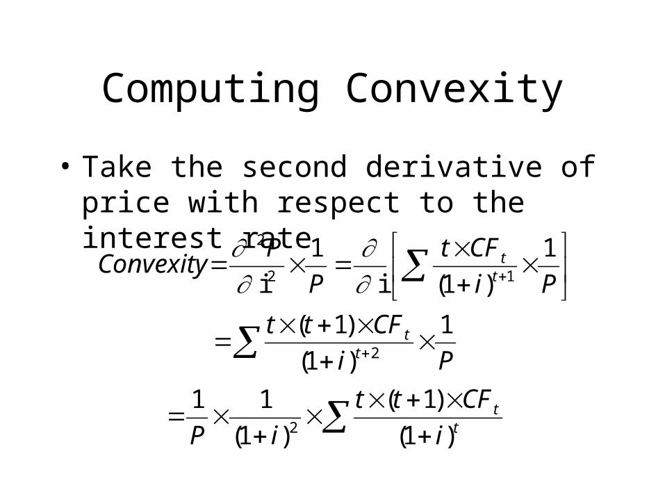
Computing Convexity
• Take the second derivative of price with respect to the interest rate
tt
tt
tt
i
CFtt
iP
Pi
CFtt
Pi
CFt
P
PConvexity
)1(
)1(
)1(
11
1
)1(
)1(
1
)1(i
1
i
2
2
12
2

Predicting Price with Convexity
• By including convexity, we can improve our estimates for predicting price
Percentage Price Change =
- Modified Duration Yield Change
+1
2Convexity (Yield Change)2
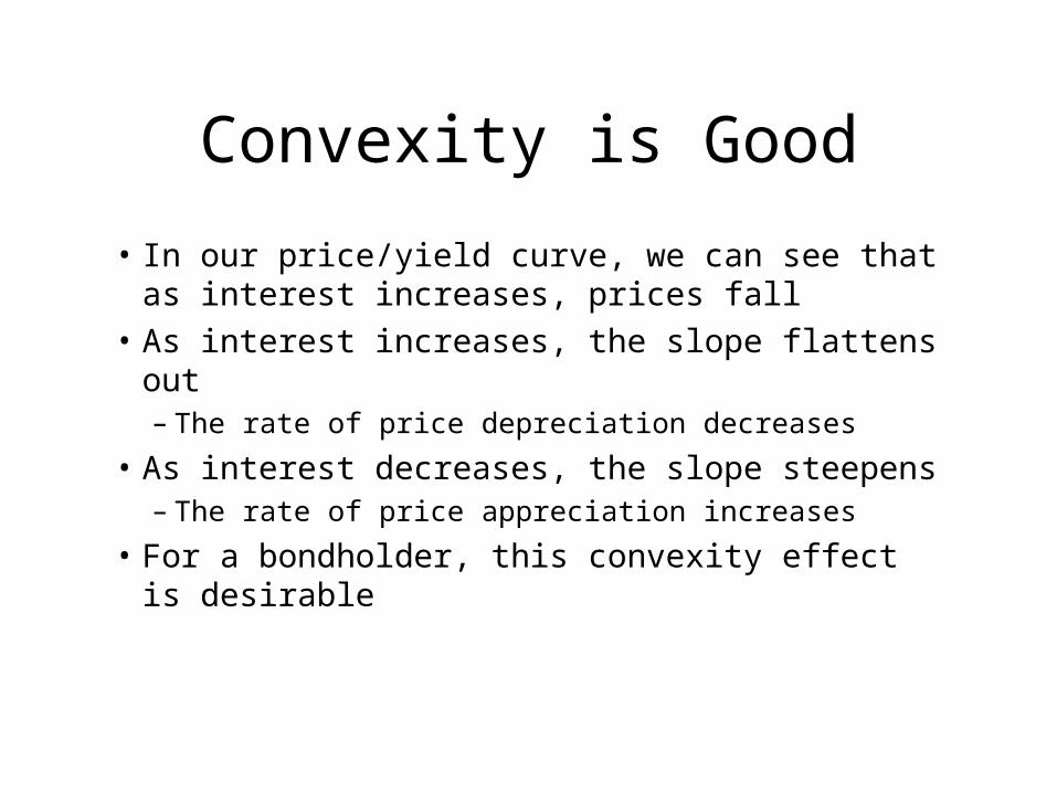
Convexity is Good
• In our price/yield curve, we can see that as interest increases, prices fall
• As interest increases, the slope flattens out– The rate of price depreciation decreases
• As interest decreases, the slope steepens– The rate of price appreciation increases
• For a bondholder, this convexity effect is desirable
Applications of Duration
• ALM evaluates the interaction of asset and liability movements
• Firms attempt to equate interest sensitivity of assets and liabilities so that surplus is unaffected– Surplus is “immunized” against interest rate risk
• Immunization is the technique of matching asset duration and liability duration
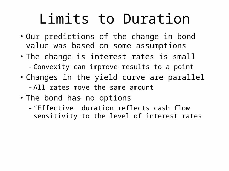
Limits to Duration• Our predictions of the change in bond value was
based on some assumptions
• The change is interest rates is small– Convexity can improve results to a point
• Changes in the yield curve are parallel– All rates move the same amount
• The bond has no options– “Effective” duration reflects cash flow sensitivity to
the level of interest rates

Assuming Parallel Shifts
• The assumption of parallel shifts in the yield curve is not plausible
• In reality, short-term rates move more than long-term rates
• Also, it is possible that the yield curve “twists”– Short-term and long-term rates move in
opposite directions
Improving Duration Measures
• Effective duration and convexity
• Term structure models
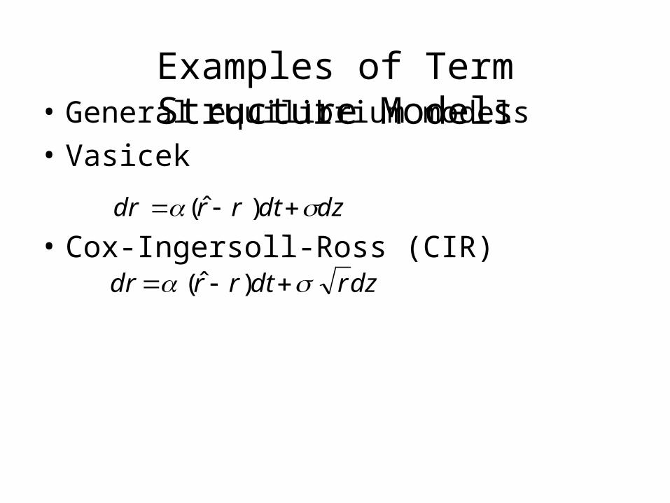
Examples of Term Structure Models• General equilibrium models
• Vasicek
• Cox-Ingersoll-Ross (CIR)dzdtrrdr )ˆ(
dzrdtrrdr )ˆ(

Arbitrage-Free ModelHeath-Jarrow-Morton
• Specifies process for entire term structure by including an equation for each forward rate
• Fewer restrictions on term structure movements
• Drift and volatility can have many forms
• Simplest case is where volatility is constant– Ho-Lee model
tdBTtfTtdtTtfTtTtdf )),(,,()),(,,(),(
Value at Risk - An Introduction• CFO of your company has just read some of the
horror stories about derivatives
• She asks you how much the company could possibly lose by using derivatives– In theory, the company could lose everything (but with
some small probability)
• How can you communicate the extent of the risk without a lecture about derivative instruments?
• Answer: Value at Risk
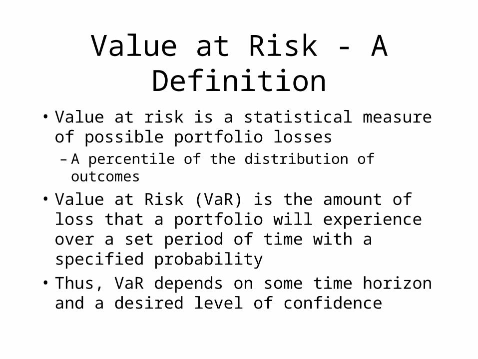
Value at Risk - A Definition
• Value at risk is a statistical measure of possible portfolio losses– A percentile of the distribution of outcomes
• Value at Risk (VaR) is the amount of loss that a portfolio will experience over a set period of time with a specified probability
• Thus, VaR depends on some time horizon and a desired level of confidence

Value at Risk - An Example• Let’s use a 5%
probability and a one-day holding period
• VaR is the one day loss that will be exceeded only 5% of the time
• It’s the tail of the return distribution
• In the example, the VaR is about $60,000
Return Distribution
VaR
($10
0,000
) $0
$100
,000
Portfolio Gains/Losses
Pro
bab
ilit
y

A Note about Value at Risk Numbers• Note that the VaR depends on the choice of time period
(t) and a probability (x)– Without knowing t and x, a value at risk number is
meaningless
• Longer t and lower x lead to higher VaR• Implicit assumption is that the portfolio is constant over
the time period t– t should be chosen to reflect portfolio trading
• x should correspond with the risk tolerance of the portfolio owner
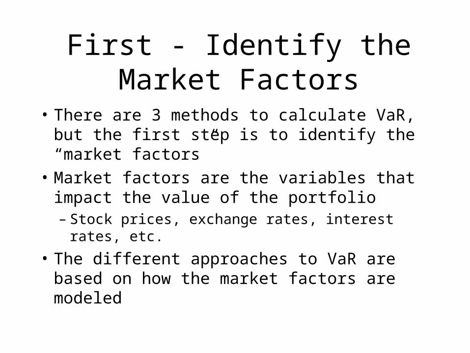
First - Identify the Market Factors
• There are 3 methods to calculate VaR, but the first step is to identify the “market factors”
• Market factors are the variables that impact the value of the portfolio– Stock prices, exchange rates, interest rates, etc.
• The different approaches to VaR are based on how the market factors are modeled
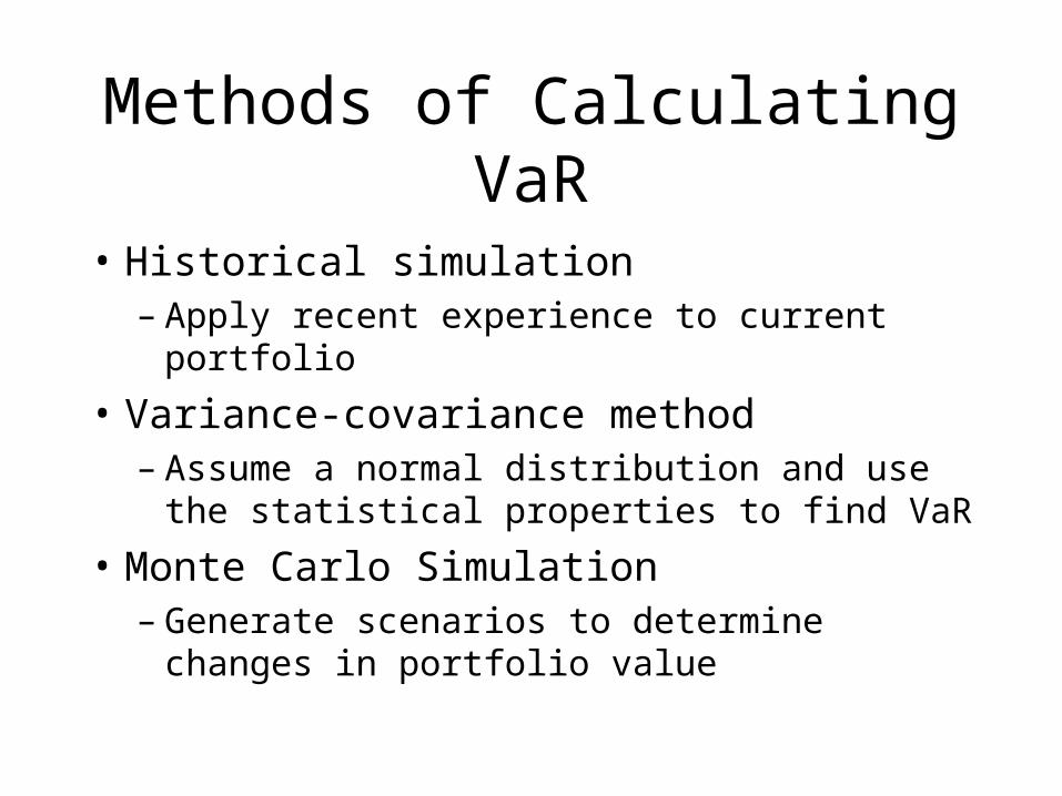
Methods of Calculating VaR
• Historical simulation– Apply recent experience to current portfolio
• Variance-covariance method– Assume a normal distribution and use the
statistical properties to find VaR
• Monte Carlo Simulation– Generate scenarios to determine changes in
portfolio value

Historical Simulation
• Use the changes in the market factors over the last 100 days (100 days is an example)
• Translate the historical experience of the market factors into percentage changes
• Apply the 100 percentage changes of the market factors to beginning portfolio values
• Rank the 100 resulting values
• VaR is the required percentile rank

Example of Historical Simulation• Assume a one-day holding period and 5% probability• Suppose that a portfolio has two assets, a one-year T-bill and a 30-year T-
bond• First, gather the 100 days of market info
Date T-Bond Value % Change T-Bill Value % Change12/10/97 102 - 97 - 12/9/97 100 2.00% 98 -1.02%12/8/97 97 3.09% 98 0.00%
: : : : : : : : : :
9/2/97 103 -2.91% 96 2.08%9/1/97 103 0.00% 97 -1.03%
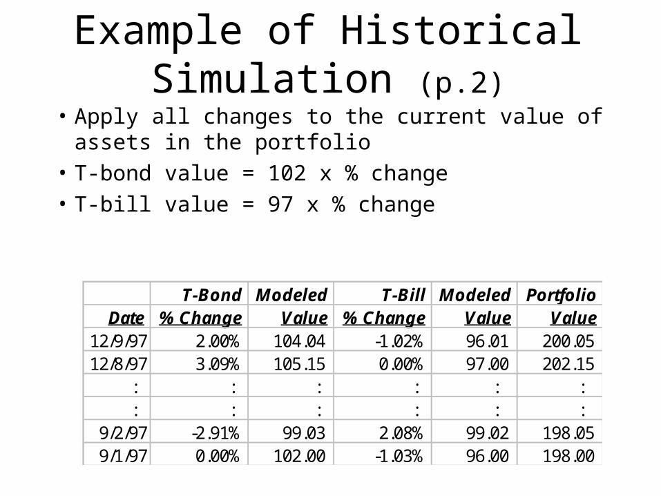
Example of Historical Simulation (p.2)
• Apply all changes to the current value of assets in the portfolio
• T-bond value = 102 x % change
• T-bill value = 97 x % change
T-Bond Modeled T-Bill Modeled PortfolioDate % Change Value % Change Value Value
12/9/97 2.00% 104.04 -1.02% 96.01 200.05 12/8/97 3.09% 105.15 0.00% 97.00 202.15
: : : : : : : : : : : :
9/2/97 -2.91% 99.03 2.08% 99.02 198.05 9/1/97 0.00% 102.00 -1.03% 96.00 198.00

• Rank the resulting 100 portfolio values
• The 5th lowest portfolio value is the VaR
Example of Historical Simulation (p.3)
PortfolioRank Date Value
1 11/12/97 195.45 2 12/1/97 196.24 3 10/17/97 197.13 4 10/13/97 197.60 5 9/1/97 198.00
: : : : : : 99 12/8/97 202.15
100 9/25/97 203.00
Notes about Historical Simulation• Historical simulation is relatively easy to do
– Only requires knowing the market factors and having the historical information
• Note that correlations between the market factors are implicit in this method because we are using historical information– In our example, short bonds and long bonds would typically
move in the same direction
• Derivative values can be modeled as a function of the underlying market factor
Variance-Covariance Method
• Assume all market factors follow a multivariate normal distribution
• Under this assumption, the distribution of portfolio gains/losses can be determined with statistical properties
• From the distribution of gains and losses, choose the required percentile to find VaR
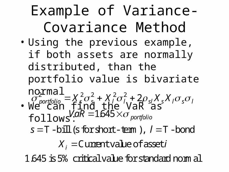
Example of Variance-Covariance Method
• Using the previous example, if both assets are normally distributed, than the portfolio value is bivariate normal
• We can find the VaR as follows:
portfolio s s l l sl s l s l
portfolio
i
X X X X
VaR
s l
X i
2 2 2 2 2 2
1645
.
,
T - bill (s for short - term) T - bond
Current value of asset
1.645 is 5% critical value for standard normal
Notes to Variance-Covariance Method
• This method is also known as the analytic method
• It is conceptually more difficult given the need for multivariate analysis
• Explaining the method to management may be as difficult as a lecture on derivatives
Monte Carlo Simulation
• In Monte Carlo simulation, we can specify the individual distributions of the future values of the market factors in the portfolio
• Generate random samples from the assumed distribution
• Determine the final value of the portfolio
• Rank the portfolio values and find the appropriate percentile to find VaR
Notes to Monte Carlo Simulation
• If the distribution of market factors is normal, Monte Carlo simulation and the variance-covariance method will give similar VaR
• Initial setup is costly, but thereafter Monte Carlo simulation can be efficient

Conclusion• Modeling is used extensively in measuring market
risk
• Interest rate sensitivity measures depend on cash flow models and term structure models
• Value-at-Risk measures can also be based on models
• Don’t be fooled by indicated precision of measures
• Understand the models underlying the calculations
Conclusion - continued
• Don’t assume best model is the one that best fits past movements
• Pick parameters that reflect current environment or view
• Recognize parameter error
• Analogy to a rabbit