Final Report

Automatic Control, Project Course

EL2421

Daniel Bug Ioannis Chatzis Anders Cioranbug@kth.se ioannisc@kth.se cioran@kth.se

Markus Fjallid Linus Flodin Anton Houfjallid@kth.se linusflo@kth.se ahou@kth.se

Kevin Kyeong Marcus Lind Simon Lundbergtaihyun@kth.se marculin@kth.se silu@kth.se

Lionel Nurwezenurweze@kth.se

January 17, 2014

Abstract

In this project, a hardware-in-the-loop (HIL) platform for developing and testing tra�ccontrol algorithms was established.

The platform consists of remote control (RC) miniature trucks, virtual models of theminiature trucks, a virtual model of a Scania truck. All these truck models are 1:14 scaleddown versions of an actual Scania truck, and the purpose of the HIL is to create tra�cscenarios with truck models which are as realistic as possible. All models interact witheach other in real-time simulation.

Using vehicle-to-vehicle (V2V) communication in which vehicles share informationabout themselves and cooperate with each other, tra�c control algorithms were devel-oped under a few scenarios. The main scenarios were a four-way crossing and a highwayentrance ramp. Other slightly less complex scenarios were also demonstrated. The plat-form is scalable and can be further improved and extended with more scenarios andcomplexities to study tra�c optimization algorithms and cooperation.

The project included ten Master’s students and took place over the course of eightweeks in the Autumn of 2013 at KTH Royal Institute of Technology in Stockholm, Swe-den.

Contents

1 Introduction 71.1 Background . . . . . . . . . . . . . . . . . . . . . . . . . . . . . . . . . . 71.2 Course Objectives . . . . . . . . . . . . . . . . . . . . . . . . . . . . . . . 71.3 Project Description . . . . . . . . . . . . . . . . . . . . . . . . . . . . . . 7

1.3.1 Description . . . . . . . . . . . . . . . . . . . . . . . . . . . . . . 71.3.2 Summary . . . . . . . . . . . . . . . . . . . . . . . . . . . . . . . 8

2 Systems Integration 92.1 Motion Capture . . . . . . . . . . . . . . . . . . . . . . . . . . . . . . . . 102.2 Miniature Trucks . . . . . . . . . . . . . . . . . . . . . . . . . . . . . . . 10

2.2.1 TMote Sky . . . . . . . . . . . . . . . . . . . . . . . . . . . . . . 112.3 xPC Target . . . . . . . . . . . . . . . . . . . . . . . . . . . . . . . . . . 11

2.3.1 Scope . . . . . . . . . . . . . . . . . . . . . . . . . . . . . . . . . 112.3.2 Communications . . . . . . . . . . . . . . . . . . . . . . . . . . . 112.3.3 Real-time Execution . . . . . . . . . . . . . . . . . . . . . . . . . 13

2.4 Main Program . . . . . . . . . . . . . . . . . . . . . . . . . . . . . . . . . 132.4.1 Front panel . . . . . . . . . . . . . . . . . . . . . . . . . . . . . . 132.4.2 Program structure . . . . . . . . . . . . . . . . . . . . . . . . . . 13

2.5 Integration . . . . . . . . . . . . . . . . . . . . . . . . . . . . . . . . . . . 142.6 Visualization . . . . . . . . . . . . . . . . . . . . . . . . . . . . . . . . . 15

2.6.1 Step 1 . . . . . . . . . . . . . . . . . . . . . . . . . . . . . . . . . 152.6.2 Step 2 . . . . . . . . . . . . . . . . . . . . . . . . . . . . . . . . . 162.6.3 Step 3 . . . . . . . . . . . . . . . . . . . . . . . . . . . . . . . . . 16

3 Map Creation 193.1 Roads . . . . . . . . . . . . . . . . . . . . . . . . . . . . . . . . . . . . . 19

3.1.1 Signs and Tra�c Lights . . . . . . . . . . . . . . . . . . . . . . . 193.1.2 Transitions . . . . . . . . . . . . . . . . . . . . . . . . . . . . . . 193.1.3 Road data . . . . . . . . . . . . . . . . . . . . . . . . . . . . . . . 20

3.2 Crossing Scenario with Transition Points . . . . . . . . . . . . . . . . . . 203.2.1 Function . . . . . . . . . . . . . . . . . . . . . . . . . . . . . . . . 203.2.2 Create transitions . . . . . . . . . . . . . . . . . . . . . . . . . . . 213.2.3 How right and left are detected . . . . . . . . . . . . . . . . . . . 213.2.4 How the CrossingMatrix is used . . . . . . . . . . . . . . . . . . . 21

3.3 Highway Scenarios with a Ramp . . . . . . . . . . . . . . . . . . . . . . . 22

2

4 Models 244.1 Miniature truck models . . . . . . . . . . . . . . . . . . . . . . . . . . . . 24

4.1.1 Velocity dynamics block . . . . . . . . . . . . . . . . . . . . . . . 244.1.2 Steering signal block . . . . . . . . . . . . . . . . . . . . . . . . . 254.1.3 Vehicle kinematics block . . . . . . . . . . . . . . . . . . . . . . . 26

4.2 Real truck model . . . . . . . . . . . . . . . . . . . . . . . . . . . . . . . 264.2.1 Drivetrain . . . . . . . . . . . . . . . . . . . . . . . . . . . . . . . 274.2.2 Control unit . . . . . . . . . . . . . . . . . . . . . . . . . . . . . . 304.2.3 Velocity controller . . . . . . . . . . . . . . . . . . . . . . . . . . 344.2.4 Steering kinematics . . . . . . . . . . . . . . . . . . . . . . . . . . 354.2.5 Limitations . . . . . . . . . . . . . . . . . . . . . . . . . . . . . . 35

5 Low Level Control 365.1 Velocity control . . . . . . . . . . . . . . . . . . . . . . . . . . . . . . . . 365.2 Trajectory Following . . . . . . . . . . . . . . . . . . . . . . . . . . . . . 36

6 High Level Control 396.1 Centralized and Decentralized Tra�c Control . . . . . . . . . . . . . . . 39

6.1.1 Tra�c Rules Hierarchy . . . . . . . . . . . . . . . . . . . . . . . . 396.1.2 Tra�c Lights and Tra�c Signs . . . . . . . . . . . . . . . . . . . 396.1.3 Tra�c Lights . . . . . . . . . . . . . . . . . . . . . . . . . . . . . 406.1.4 Tra�c Signs . . . . . . . . . . . . . . . . . . . . . . . . . . . . . . 416.1.5 Right-hand Rule . . . . . . . . . . . . . . . . . . . . . . . . . . . 41

6.2 Collision Avoidance . . . . . . . . . . . . . . . . . . . . . . . . . . . . . . 426.3 Vehicle-To-Vehicle Communication . . . . . . . . . . . . . . . . . . . . . 446.4 Crossing Scenario . . . . . . . . . . . . . . . . . . . . . . . . . . . . . . . 44

6.4.1 Information exchange . . . . . . . . . . . . . . . . . . . . . . . . . 446.4.2 Algorithm . . . . . . . . . . . . . . . . . . . . . . . . . . . . . . . 45

6.5 Highway Entrance Scenario . . . . . . . . . . . . . . . . . . . . . . . . . 466.5.1 Information exchanges . . . . . . . . . . . . . . . . . . . . . . . . 476.5.2 Algorithm . . . . . . . . . . . . . . . . . . . . . . . . . . . . . . . 476.5.3 Problems . . . . . . . . . . . . . . . . . . . . . . . . . . . . . . . 48

7 Conclusions 50

8 Suggestions for future work 518.1 Models and Control . . . . . . . . . . . . . . . . . . . . . . . . . . . . . . 51

8.1.1 Models . . . . . . . . . . . . . . . . . . . . . . . . . . . . . . . . . 518.1.2 Control . . . . . . . . . . . . . . . . . . . . . . . . . . . . . . . . 51

8.2 Tra�c Control . . . . . . . . . . . . . . . . . . . . . . . . . . . . . . . . . 528.2.1 Crossings . . . . . . . . . . . . . . . . . . . . . . . . . . . . . . . 528.2.2 Highway Entrance . . . . . . . . . . . . . . . . . . . . . . . . . . 52

8.3 System integration . . . . . . . . . . . . . . . . . . . . . . . . . . . . . . 528.3.1 Visualization . . . . . . . . . . . . . . . . . . . . . . . . . . . . . 528.3.2 xPC Target . . . . . . . . . . . . . . . . . . . . . . . . . . . . . . 52

A Purchase Order 55

B Scania GCDC CAN Messages 61

3

C Data Packets 63C.1 Main Program to Visualization tool . . . . . . . . . . . . . . . . . . . . 63

D Real truck model data 66

4

List of Figures

2.1 SML Environment. . . . . . . . . . . . . . . . . . . . . . . . . . . . . . . 92.2 Miniature RC Truck of a Scania Model. . . . . . . . . . . . . . . . . . . . 102.3 xPC Target Platforms . . . . . . . . . . . . . . . . . . . . . . . . . . . . 122.4 Frontpanel of the main program . . . . . . . . . . . . . . . . . . . . . . . 132.5 Flowchart of the main program . . . . . . . . . . . . . . . . . . . . . . . 142.6 Diagram over system interface . . . . . . . . . . . . . . . . . . . . . . . . 172.7 Graphical userinterface of the visualization tool. . . . . . . . . . . . . . . 18

3.1 Map example with waypoints. . . . . . . . . . . . . . . . . . . . . . . . . 203.2 Crossing map example. . . . . . . . . . . . . . . . . . . . . . . . . . . . . 223.3 Highway entrance example. . . . . . . . . . . . . . . . . . . . . . . . . . 23

4.1 The miniature truck model. . . . . . . . . . . . . . . . . . . . . . . . . . 244.2 Velocity dynamics block. . . . . . . . . . . . . . . . . . . . . . . . . . . . 254.3 Steering block structure. . . . . . . . . . . . . . . . . . . . . . . . . . . . 254.4 Bicycle kinematic model. . . . . . . . . . . . . . . . . . . . . . . . . . . . 274.5 Drivetrain model. . . . . . . . . . . . . . . . . . . . . . . . . . . . . . . . 284.6 Available engine torque. . . . . . . . . . . . . . . . . . . . . . . . . . . . 294.7 Shift decision logic. . . . . . . . . . . . . . . . . . . . . . . . . . . . . . . 324.8 Velocity controller (Real truck model). . . . . . . . . . . . . . . . . . . . 34

5.1 Trajectory following. . . . . . . . . . . . . . . . . . . . . . . . . . . . . . 375.2 FIR steering controller (de)activation. . . . . . . . . . . . . . . . . . . . . 38

6.1 Sorted crossing and placement of tra�c lights/signs . . . . . . . . . . . . 406.2 Alternating of tra�c lights in a crossing . . . . . . . . . . . . . . . . . . 406.3 Illustration of the collision controller . . . . . . . . . . . . . . . . . . . . 426.4 A standard ellipse, with the radii a and b. . . . . . . . . . . . . . . . . . 436.5 Sections in crossing. . . . . . . . . . . . . . . . . . . . . . . . . . . . . . . 446.6 Highway entrance scenario. . . . . . . . . . . . . . . . . . . . . . . . . . . 466.7 General communication setup. . . . . . . . . . . . . . . . . . . . . . . . . 476.8 General decision algorithm. . . . . . . . . . . . . . . . . . . . . . . . . . 48

B.1 Simulink Block Sets for GCDC20 CAN Message . . . . . . . . . . . . . . 61B.2 Simulink Block Sets for GCDC00-07 CAN Messages . . . . . . . . . . . . 62

5

List of Tables

3.1 Contents of the file SignInfo.txt . . . . . . . . . . . . . . . . . . . . . . . 213.2 CrossingMatrix Column Information. . . . . . . . . . . . . . . . . . . . . 21

4.1 Gear state description I. . . . . . . . . . . . . . . . . . . . . . . . . . . . 314.2 Gear state description II. . . . . . . . . . . . . . . . . . . . . . . . . . . . 314.3 Gear state update. . . . . . . . . . . . . . . . . . . . . . . . . . . . . . . 324.4 Gear shifting procedure. . . . . . . . . . . . . . . . . . . . . . . . . . . . 33

6.1 Shared collision matrix. . . . . . . . . . . . . . . . . . . . . . . . . . . . . 456.2 Crossing example. . . . . . . . . . . . . . . . . . . . . . . . . . . . . . . . 45

D.1 Scania model parameters. . . . . . . . . . . . . . . . . . . . . . . . . . . 66D.2 Scania model gear ratios. . . . . . . . . . . . . . . . . . . . . . . . . . . . 67

6

Chapter 1

Introduction

1.1 Background

Cooperation between vehicles can enable safer, greener and more e�cient tra�c andtransports. Vehicles can communicate their states, such as velocity and position, andhence adapt to the surrounding tra�c in order to avoid collision and optimize tra�c incrossings, for instance. This adaptation can be done autonomously for a large number ofvehicles which will give us a more e�cient tra�c.

To develop this system of cooperation, a simulation platform needs to be built inorder to evaluate the cooperation. Such a platform and cooperation will be described inthis report.

1.2 Course Objectives

The course EL2421 Automatic control, project course is a 15-credit course running overten weeks. In the course of 2013, ten Master’s students with various engineering disci-plines are taking the course. The course aims to teach the students to work in projectsand give practical knowledge about modelling and design of control systems.

The course takes place in the Smart Mobility Lab (SML) at the Royal Institute ofTechnology (KTH) in Stockholm, Sweden. A new project is created for every year’scourse and the result is supposed to contribute to the lab.

1.3 Project Description

This section will give a short description of the project goals. To access the purchasedorder given to the group at the beginning of the project, please see Appendix A

1.3.1 Description

The project aims to develop a hardware-in-the-loop simulation platform including bothradio controlled real miniature trucks and simulated models of trucks.

7

Trucks

The SML possesses radio controlled miniature trucks. For this simulation, truck modelsshould be developed for a LabVIEW environment as well as external real time hardware(xPC). Steering and velocity controllers should be built for all trucks.

All types of trucks should be able to drive on the same road network at the same timeand in the end be able to interact which each other. The miniature truck models shouldhave the same behavior as the real miniature trucks and enable to more easily simulatecomplex scenarios without risk of damages due to collisions with real trucks. The fullscale Scania truck models behavior correspond to a real truck and can for example helpto get a more reality-like scenario.

Control Complexities and Scenarios

Several simulation with di↵erent scenarios and di↵erent levels of tra�c control will bedeveloped. The most advanced scenario include vehicle-to-vehicle communication wheretrucks cooperate, share information and negotiate on what action they will take. Thiscooperation needs to be developed. To test the cooperation it will be implemented intwo scenarios: a four way crossing and a highway entrance ramp.

There will be three levels of tra�c control complexities implemented (taken from thepurchased order, see Appendix A): 1) Centralized tra�c control, using tra�c lights;2) Decentralized controlled based on tra�c rules and pre-defined priorities, for examplethe right-hand rule; 3) Cooperative decisions where vehicles agree on their actions, nopredefined priorities or rules.

1.3.2 Summary

The following is a summary of the order given to the group:

• Design kinematic/dynamic models of the miniature trucks and run them in Lab-VIEW

• Design a model of a full scale truck and run it on a dedicated xPC target

• Run simulations in real time

• Create an integrated hardware-in-the-loop simulation environment

• Create vehicle controllers for steering and velocity

• Create communication between vehicles

• Create tra�c controllers with di↵erent levels of complexities

• Implement tra�c control in di↵erent scenarios

• Visualize the simulation

8

Chapter 2

Systems Integration

Prior to getting into the details of truck modeling and tra�c control scenarios, this chapterintroduces di↵erent systems installed in the SML, and presents their functionalities andsetups. The integration of the systems and their purposes in real world environment arealso discussed.

As shown in Figure 2.1, the major components in the SML are motion capture cam-eras, miniature RC trucks, xPC Target machines, main program in LabVIEW, visualiza-tion tool in MATLAB, and ceiling mounted projectors.

Figure 2.1: SML Environment.

The motion capture cameras are from Qualysis and are handled by Qualisys TrackingManager (QTM). They are used to track the motion of the miniature RC trucks in thelaboratory environment.

9

The xPC Target machines are real-time systems that run a real life truck model andits self-driving controller. When it comes to the study of the performance of a truck invarious tra�c scenarios, this is perhaps the core part of the whole platform.

Then, to create more interesting tra�c flow, the miniature trucks are modelled inequations and virtualized in the main LabVIEW program. It is also this LabVIEW pro-gram where various tra�c controls are implemented and all communications between thesystems are handled to establish a hardware-in-the-loop (HIL) platform. If the purposeof xPC Target is to study the characteristics of a real truck, the main LabVIEW programis used to study and experiment di↵erent tra�c control algorithms.

Finally, the visualization tool in MATLAB is used to project road networks, virtualmini-trucks and simulated real life trucks on the floor of the SML for demonstration.Furthermore, a secondary projector serves as the dashboard of the simulated real truckmodel.

2.1 Motion Capture

The SML is equipped with 12 motion capture cameras placed on the ceiling in such away that the area where objects are to be tracked is well covered by the cameras. Themotion capture system then tracks the motion of objects in this designated area by usinginfrared reflective markers placed on the objects. Each object has the markers on themwith a unique spatial pattern, and such is defined and stored in the QTM. In the scopeof this project, the motion capture system has mainly been used for positioning feedbackof RC trucks that are included in tra�c scenario demonstrations. The detailed guides onsetting up and using this system have previously been worked on by the SML techniciansMani, Pedro and Joao, and can be referred to their manuals for more information[2][5].

2.2 Miniature Trucks

In the lab, there are several remote control (RC) trucks which are 1:14 scaled downversions of a Scania truck like the one shown in Figure 2.2. These are battery operatedand TMote Sky is installed on each of these miniature truck instead of the originallyprovided RC device.

Figure 2.2: Miniature RC Truck of a Scania Model.

10

2.2.1 TMote Sky

TMote Sky is a wireless sensor platform for low-power, high data-rate sensor networkapplications. It consists of two electric circuit boards: one is placed on either a movingobject or a remote station, and the other is usually attached to the central processingstation where information from multiple TMote Sky circuits can be collected and shared.The details about the use of TMote Sky and its software TinyOS have also been docu-mented by the aforementioned SML technicians and can be referred to their manuals formore information[2][5].

2.3 xPC Target

xPC Target is a product from MathWorks, and basically is a real-time software environ-ment that allows one to run Simulink and Stateflow models on any x86-based real-timesystems. Without having to build or test on a real physical model, a system of interestcan be modeled, simulated and studied using xPC Target.

A Scania truck model is thus simulated on an xPC Target hardware platform andcontroller algorithms are implemented and tested on this virtual model instead of a realtruck.

2.3.1 Scope

In the Automatic Control department of KTH, there had been some work done on xPCTarget as part of Stockholm Cooperative Driving Project (Scoop). In the Scoop, however,xPC Target was used only to develop a self-driving controller[3]. The scope of the EL2421project extends this to have an xPC Target platform that represents a real life truck modelas accurately as possible. The benefit of this suggested platform is that as the modelshould well represent an actual truck, it can give out all kinds of physical characteristics ofthe truck under di↵erent tra�c scenarios. One of the important and useful characteristicsthat can be obtained is fuel e�ciency with a particular control algorithm applied on thetruck platform.

2.3.2 Communications

In this project, two xPC Target platforms have been used: one to virtualize a Scania truckmodel, and the other to rapid prototype a self-driving controller for the Scania truck.These two systems communicate with each other via controller area network (CAN) andthis configuration is completely identical to the connection between a Scania truck andits main electronic control unit (ECU). Thus, xPC Target allows one to fully simulate asystem including small details like communication protocols between its subsystems.

The CAN message protocol used in this project has been identical to that of GrandCooperative Driving Challenge (GCDC) in which the Automatic Control departmentof KTH participated in cooperation with Scania. For the details of the messages, seeAppendix B.

CAN

There are 9 GCDC CAN messages, namely GCDC00, 01, 02, 03, 04, 05, 06, 07, 20.Among them, GCDC20 gets sent to the truck from the controller, and the rest is received

11

Figure 2.3: xPC Target Platforms

by the controller from the truck.In GCDC20, in replacement of ExternalAccelerationDemand, a new variable called

SteeringAngleReference was defined.The xPC Target systems are equipped with CAN I/O functionalities and a CAN

bus between systems is established by using Simulink block instances. For the xPCTarget platform on a custom PC, the CAN I/O board is Softing CAN-AC2-PCI, andcorresponding CAN Simulink block instances are included in the installation of Simulink’sxPC Target toolbox. On the other hand, the Speedgoat machine requires an additionalinstallation of its own xPC Target toolbox.

When establishing a CAN bus, it is also critical to define what each message containsand how the data in each message is organized. Using provided CAN Simulink block sets,the message format can be manually edited. Nonetheless, there is a more convenient wayof doing this, which is creating a single CAN database (*.dbc) and having each CAN nodeto refer to this database. This way, any future modification to the protocol can be mademore readily and any sort of inconsistency between CAN block sets can be minimized.The CAN database was created using CANdb++ editor by Vector.

To ease the learning curve and development time in any future projects on xPC Target,simple examples and debugging tools have been created (see the file HelloCAN.slx ).

UDP

Besides CAN, one of other communication protocols available on xPC Target is userdatagram protocol (UDP). The internet protocol TCP is not supported by xPC Targetas it does not have the nature of real-time that UDP does.

This communication protocol was used to simulate the built-in wireless communica-tion system in Scania trucks. In the lab environment, this was simply to communicatebetween xPC and the main LabVIEW program.

12

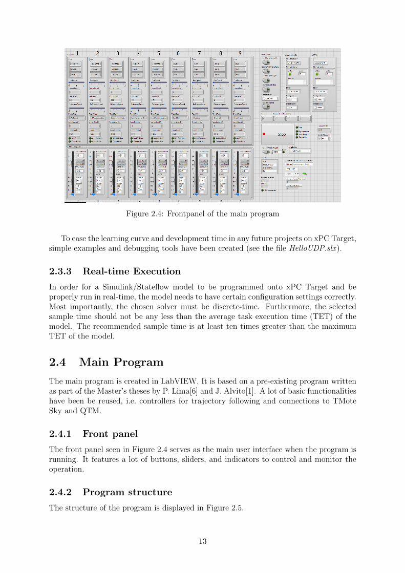
Figure 2.4: Frontpanel of the main program

To ease the learning curve and development time in any future projects on xPC Target,simple examples and debugging tools have been created (see the file HelloUDP.slx ).

2.3.3 Real-time Execution

In order for a Simulink/Stateflow model to be programmed onto xPC Target and beproperly run in real-time, the model needs to have certain configuration settings correctly.Most importantly, the chosen solver must be discrete-time. Furthermore, the selectedsample time should not be any less than the average task execution time (TET) of themodel. The recommended sample time is at least ten times greater than the maximumTET of the model.

2.4 Main Program

The main program is created in LabVIEW. It is based on a pre-existing program writtenas part of the Master’s theses by P. Lima[6] and J. Alvito[1]. A lot of basic functionalitieshave been be reused, i.e. controllers for trajectory following and connections to TMoteSky and QTM.

2.4.1 Front panel

The front panel seen in Figure 2.4 serves as the main user interface when the program isrunning. It features a lot of buttons, sliders, and indicators to control and monitor theoperation.

2.4.2 Program structure

The structure of the program is displayed in Figure 2.5.

13

Figure 2.5: Flowchart of the main program

When the program is started, the following initialization phase takes place.

• Variables are initiated

• Road network files are read in to the memory

• Initial positions for the simulate vehicles are calculated

The three following branches in the flow represent processes running in parallel i.e.asynchronous. The uppermost branch is what is referred to as the main loop.

Get positions updates x,y and yaw position variables for each active vehicle. Positionsfor real Mini Trucks are collected from the motion capture system, positions for simulatedMini Trucks are collected from the parallel process Simulation loop and positions for thesimulated Scania Truck are collected from the XPc target machine through the UDPreceiver process.

Tra�c control process runs di↵erent tra�c control algorithms depending on settingsin the front panel. The algorithm runs in a for-loop that iterates once for each vehicle.The inputs are vehicle position, desired speed from front panel, road network etc. Theoutputs are a reference speed and waypoint.

The Vehicle control process uses the outputs from Tra�c control as references forspeed and steering controllers.

In Send control data the control values from Vehicle control are transferred to corre-sponding vehicle.

The main loop is also part of the actual control loop. The sampling time T

s

is set byaltering a time delay in the Send control data process.

2.5 Integration

The separate devices in the system are connected using internet protocols (IPs). Anoverview of the setup can be seen in Figure 2.6 and packet structures are listed in Ap-pendix C.

The motion capture system is connected to the Main Program using TCP. In theMain Program the connection is handled within a closed LabVIEW library provided byQualisys.

Problems were detected when a LabVIEW program receives UDP packets from thexPC. For an unknown reason the reception rated dropped to about one packet in five

14

seconds. A simple port forwarder is implemented as a workaround for this issue. The portforwarder is written in Python and is running on the same computer as the LabVIEWprogram, i.e. Main Program and xPC monitor. It receives a packet on specified UDPport and forwards it to another UDP port on the localhost.

2.6 Visualization

The visualization tool is entirely written in MATLAB. It receives the map to projectfrom the LabVIEW computer using TCP/IP transmission and the data used for display-ing the trucks are received using UDP. A local copy of the map can also be loaded butit is important to always use the same map as LabVIEW. The code for the visualizationtool is based on Jonathan and Eriks summer project [7].

The graphical user interface is divided in three logical steps as shown in Figure 2.7. Allthe di↵erent buttons and inputs of the interface are described in the proceeding sections.When the projection button in the third step is pressed the graphical map is generated.From the packets received from LabVIEW overlaying graphics is generated. This includestra�c lights, trucks and informative texts. When a new UDP package is received fromLabVIEW the overlaid graphics representing the trucks etc. are updated to the newestpositions and states. The framerate is decided by the speed of which LabVIEW is sendingthe UDP packages. The maximum framerate is however limited by how fast MATLABcan update the graphical objects. Experiments have shown that around 30 frames persecond is maximum in our setup.

2.6.1 Step 1

In the first step general settings are applied regarding appearance and network connection.

Show waypoints Display arrows on all the waypoints if ticked.

Show Bridge Not used.

Show static map (without trucks) If ticked only the map will be displayed. Notrucks are shown.

Hide physical trucks Hides the blue box for the physical trucks if ticked.

Add marker in origo Shows a cross in origo if ticked. Useful for calibration and cen-tering.

Run on same PC as LabVIEW If ticked the program will listen for data on the lo-calhost.

Jonas mode All trucks are replaced with images of Jonas.

Color theme Select a color theme for the projection.

IP Host Computer IP address of the computer transmitting the map and sendingtruck data.

UDP receive port This specifies on which port the truck data is received on.

15

2.6.2 Step 2

In the second step one reads the map either from a local copy or received from LabVIEW.

Load local map Reads a local copy of a map saved on the computer.

Host Computer port Specifies which port to use for the TCP/IP transmission.

Transfer map via TCP/IP Click this button to receive an pending map transmissionfrom LabVIEW.

Map received Indicates that all files needed for the map has been received.

2.6.3 Step 3

In the third step the actual projection is started by pressing the huge button. A newfigure appears on the secondary monitor.

16

Figure 2.6: Diagram over system interface

17

Figure 2.7: Graphical userinterface of the visualization tool.

18

Chapter 3

Map Creation

One advantage with a good simulation platform is the ability to rapidly change scenariosand tra�c situations. The map creation tool, Road Network Creator, inherited from theprevious project, has been used [7]. This chapter will describe how roads are created fordi↵erent scenarios and what is important to take into account. It will also give a briefexplanation of files and information associated with the road network that the simulationplatform uses.

3.1 Roads

The road is represented by waypoints which are interpolated between manually placedmarks in the Road Network Creator. Each waypoint has a number, starting from zero,and an associated x- and y-coordinate. Figure 3.1 shows an example where every pointrepresents a waypoint.

When creating a road network, several files are created of which some are explainedhere.

3.1.1 Signs and Tra�c Lights

Several tra�c signs are implemented and can be used. Signs are associated with a way-point which, if necessary, can be changed manually in the file SignInfo.txt. Every columnin this file represents a sign and includes the information in Table 3.1

Tra�c light information is stored in the file TLInfo.txt and includes information aboutroad number, waypoint and coordinates [7].

3.1.2 Transitions

Transitions are a way to change road, turn or make a shortcut between waypoints. Eachtransition starts with a FromState and ends with a ToState. Transition point data arestored in the file TransitionMatrix.txt. Every transition has a number represented by thecolumn, line one and two tell us which road the FromState is and its waypoint number.Line three and four give the same information but about the ToState.

19

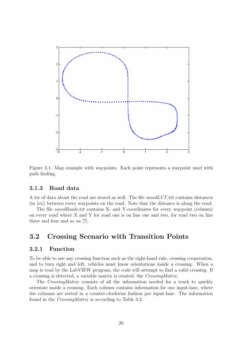
Figure 3.1: Map example with waypoints. Each point represents a waypoint used withpath finding.

3.1.3 Road data

A lot of data about the road are stored as well. The file savedLUT.txt contains distances(in [m]) between every waypoints on the road. Note that the distance is along the road.

The file savedRoads.txt contains X- and Y-coordinates for every waypoint (column)on every road where X and Y for road one is on line one and two, for road two on linethree and four and so on [7].

3.2 Crossing Scenario with Transition Points

3.2.1 Function

To be able to use any crossing function such as the right-hand rule, crossing cooperation,and to turn right and left, vehicles must know orientations inside a crossing. When amap is read by the LabVIEW program, the code will attempt to find a valid crossing. Ifa crossing is detected, a variable matrix is created, the CrossingMatrix.

The CrossingMatrix consists of all the information needed for a truck to quicklyorientate inside a crossing. Each column contains information for one input-lane, wherethe columns are sorted in a counter-clockwise fashion per input-lane. The informationfound in the CrossingMatrix is according to Table 3.2.

20

Table 3.1: Contents of the file SignInfo.txt

Information NotesRoad

WaypointX-coordinateY-coordinateType of sign 1=Stop, 2=Yield, 3=Velocity, 4=Pedestrian crossingVelocity Only for velocity signs

Table 3.2: CrossingMatrix Column Information.

Row number Column information1 FromState Road number2 FromState Way Point number3 ToState Road number (Transition point row 1)4 ToState Way Point number (Transition point row 1)5 Next Road number if RIGHT Turn6 Next Way Point number if RIGHT Turn7 Next Road number if LEFT Turn8 Next Way Point number if LEFT Turn

3.2.2 Create transitions

When creating a four-way crossing, one needs to place exactly four transition points inthe crossing area. The four transition points must be placed in such a way that all statesseen in Figure 3.2 are covered, where the from-states and to-states match. Note thatthere should be no transition point beginning or ending inside the crossing.

The road that was used for testing had the shape of an infinity-loop with a two-waysingle-lane road. However, any road configuration could work, as long as the transitionpoints are set correctly.

The program is coded to detect four transition points in vicinity to each other, whichis the main condition for it to detect a crossing.

3.2.3 How right and left are detected

If transition points are placed correctly, the program will be able to create the Cross-ingMatrix. Every entrance (FromState) to the crossing is represented by a column andevery column contains information about what road and waypoint (ToState) the vehiclehas on its right and left.

The program compares the X- and Y-coordinate of the ToStates and by finding theextreme values it is able to sort them in an anti-clockwise direction. From this theToStates, to the right and left are sorted into the CrossingMatrix.

3.2.4 How the CrossingMatrix is used

When a vehicle is approaching a crossing and intends to follow a tra�c rule or turn itchecks the CrossingMatrix for a column that corresponds with its own position (road and

21

Figure 3.2: A crossing map created in the map-creator with indicated points for the fourtransition points. Each line represents a road.

waypoint). When it finds it, it can easily detect what waypoints is on its right and leftside.

If a transition point is located at a waypoint before a tra�c light or sign and thevehicle intends to turn it will not react to the sign/light. Make sure that the tra�c lightor sign is located at a waypoint in front of the transition and if necessary manually changethe transition point.

3.3 Highway Scenarios with a Ramp

The highway entrance scenario requires at least two roads, a yield sign and a transitionpoint. A highway entrance is detected if and only if there is an yield sign followed (within50 waypoints) by a transition point from the same road. The transition point will thenact as the entrance point from the regular road to the highway road. Therefore, the tworoads should preferably be very close to each other (almost overlapping) at the transitionpoint.

Because of how the implemented algorithm works, the transition point should bepositioned near the end of a straight road section where the two roads go in parallel.

As an example, the road structure as in Figure 3.3 for testing the scenario was used.For more realistic performance, it is also suitable to add speed signs wherever neces-

sary. Suggestively, a high speed sign on the highway and one close to the yield sign, anda lower speed sign at the beginning of the regular road.

22

Figure 3.3: Example of a suitable highway entrance map created inRoad Network Creator. Outer road: highway, inner road: regular road. The sec-ond transition point is for testing purposes (for setting trucks back on the inner roadafter having existed to the outer road).

23

Chapter 4

Models

Di↵erent types of vehicles are used in the simulation platform, each with their ownadvantages and disadvantages. This chapter will describe the two di↵erent models usedand developed: The miniature truck models and the real truck model.

4.1 Miniature truck models

The miniature truck model captures the simple dynamics of Tamiya RC Scania R620,taking into account some physical limits. No gearing is taken into consideration, sincethe miniature trucks in the experiments only drive on one gear as well. The miniaturetruck model block is illustrated in Figure 4.1.

Velocity dynamics

Steering signal

Kinematics�ref

[x, y, �]

vref

Figure 4.1: The miniature truck model.

The inputs to the model are the velocity, vref and steering angle, �ref signals, whilethe outputs are the position of the miniature trucks (x, y) and the yaw angle ✓. Theminiature truck model consists of three main blocks: a) The velocity dynamics block;b) the steering signal block; and the c) vehicle kinematics block.

4.1.1 Velocity dynamics block

The structure of the velocity dynamics block is portrayed in Figure 4.2. The velocitydynamics block consists of the following three sub-blocks:

• The communication delay block

• The saturation block

• The first-order velocity dynamics block

24

Communicationdelay

vrefSaturation First-order

velocity dynamics

vref

Figure 4.2: The structure of the velocity dynamics block.

Communication delay block

The communication delay block models the time required for the input signal vref to reachthe receiver in the miniature truck through the wireless link. The communication delay,tdelay used in the project is tdelay = 0.16 [s] [4].

Saturation block

The saturation block models the minimum and maximum velocity vmin and vmax respec-tively, the miniature trucks can achieve. The upper limit of the saturation block whichcorresponds to the maximum attainable velocity is vmax = 2 [m/s] while the lower limitis vmin = 0 [m/s], which is corresponding to the lowest attainable velocity [4].

First-order velocity dynamics block

The first-order velocity dynamics block models the inertia of the miniature truck whichlimits the rate of change of the velocity. It is represented by a first-order transfer functionF (s) such that:

F (s) =1

⌧s+ 1(4.1)

where ⌧ is the time constant. The time constant used in the project is ⌧ = 0.3 [s] wasmanually adapted to match the real trucks behavior.

4.1.2 Steering signal block

The structure of the steering signal block is portrayed in Figure 4.3. The steering signalblock consists of the following four sub-blocks:

• The communication delay block

• The saturation block

• The rate limiter block

• The backlash block

Communicationdelay Saturation Rate limiter Backlash

�ref ˜�ref

Figure 4.3: The structure of the steering signal block.

25

Communication delay block

The communication delay block serves the same way as the one included in the velocitydynamics block and as a result has the same value tdelay = 0.16 [s].

Saturation block

The saturation block models the minimum and maximum steering angles, �min and �max

respectively, the miniature trucks can achieve. The upper limit of the saturation blockwhich corresponds to the maximum left steering angle is �max = 0.4 [rad], while the lowerlimit is �min = �0.4 [rad], corresponding to the maximum achievable right steering angle.These limits where determined by measuring the maximum and minimum steering angleof the miniature trucks.

Rate limiter block

The rate limiter block limits the rate of change of the steering angle �. The limits of therate limiter block are ±365 [rad/s] [4].

Backlash block

Finally, the backlash block models the deadzone before a change from a positive to anegative steering angle is applied and vice versa. The deadband of the backlash blockused in the project is � = 0.02 [rad] which is the 5% of the maximum steering angle�max.

4.1.3 Vehicle kinematics block

The kinematic vehicle model used for the trucks is the bicycle model. The bicycle modelis illustrated in Figure 4.4. Assuming that the velocity v is constant the bicycle model isdescribed by Equation 4.2 - Equation 4.4.

x (t) = v (t) cos (� (t) + ✓ (t)) (4.2)

y (t) = v (t) sin (� (t) + ✓ (t)) (4.3)

✓ (t) =v (t)

l

tan� (t), (4.4)

where x and y are the Cartesian coordinates of the rear position of the miniature truck,✓ and � are the yaw and steering angle respectively, v is the miniature truck velocity, l isthe length between the axles of the miniature truck, and ✓ is the yaw rate.

4.2 Real truck model

In this section, the model of the real truck that is simulated in real time on the xPC isexplained. The purpose of the model is to make it possible to see how a real truck wouldbehave in the system. To do this, a model is created in Simulink including the di↵erentcomponents of a real truck drivetrain and related control systems.

As a way to obtain realistic values on parameters, Scania provide the project withdata that is logged in an actual truck when driving. Some of the parameters in the model

26

x

y

�

�v

l

Figure 4.4: The bicycle kinematic model.

can then be identified in this way, which makes it possible to create a better model.Besides this, some parameter values are obtained directly from Scania.

4.2.1 Drivetrain

The drivetrain of a truck can be divided into several main components, see Figure 4.5,including engine, clutch, gearbox and di↵erential. This part of the model captures howthe torque from the engine is transferred to the wheels and thus to the vehicle body. Theinput to this part of the model is the actual throttle level, � and the brake level, �. Thesesignals are limited so that �, � 2 [0, 1], where the upper limit implies full throttle/brake.

The drivetrain is modeled using the physical modeling toolbox, Simscape, withinSimulink. This means that the drivetrain is connected in a physical network conservingthe power as it is transferred between the components.

In physical modeling one often talks about through and across variables. A throughvariable is transmitted through an element in the system, for example current that istransferred through one side to the other in a resistor. An across variable is the di↵erencebetween two points in an element, for example voltage that is the di↵erence between twolevels of potential.

Since the product of the variables has the unit of power, they can be related by aset of equations in every element in a way so that the power is always conserved in thephysical network.

In the drivetrain model, these variables are torque and angular velocity respectivelyexcept for the last part of the drivetrain model which converts the power in to thetranslational domain with force and translational velocity.

The gearing system is modeled as semi automatic, which is often the case in real trucks.This means that there is a clutch and a gearbox which are controlled automatically by a

27

control system. The commands from a driver or, as in this case, the velocity controlleris therefore an accelerator signal and a brake signal.

Figure 4.5: Drivetrain model.

Engine

The engine is modeled using an ideal torque source together with a look up table for theavailable torque. See Figure 4.6 for the data that is used in the model. The look uptable provides the available maximum torque from the engine at current engine speed,Tmax(nengine), which is then multiplied by the throttle level. Some engine friction, Tfriction

is subtracted to give the actual torque. The engine model also includes an inertia, Jengine.The engine dynamics can therefore be described by the following set of equations whenstandalone.

Jengine!engine = T

max

(nengine)� � Tfriction, (4.5)

where !engine is the angular speed of the engine. The engine speed and actual torque aremeasured for use by other parts of the system.

Numerical values used in this part of the model are Jengine = 65.8 [kg/m2] [?] togetherwith the engine torque data obtained from Scania. Tfriction is set to 50 [Nm] in order to geta realistic deceleration of engine speed when disconnected from the rest of the drivetrain.

Clutch

The purpose of the clutch is to make it possible to control the torque that is transferredfrom the engine to the rest of the drivetrain. This enables starting from standstill anddecoupling of the engine when shifting gear. This component is modeled using a disk fric-tion clutch component in Simscape, which models how the torque is transferred betweentwo shafts by friction between two or more rotating surfaces.

The torque transferred by the clutch is proportional to the clutch pressure, Pclutch

,which is controlled by the control unit. The control signal is a value in the range [0,1],where 1 implies full pressure and thus maximum torque transferred.

The maximum pressure required in order to be able to transfer maximum torque fromthe engine is calculated by inverting the clutch model1. This means that the clutch isable to transfer this torque independent on the clutch parameters, which are set to thedefault values in Simulink.

This component also features a clutch slip sensor, making the di↵erence in angularspeed between the input and output shaft available to other parts of the model.

1See the help section in Simulink.

28

0 500 1000 1500 2000 25000

500

1000

1500

2000

2500

Torq

ue[N

m]

S p e ed [rpm ]

Figure 4.6: Available engine torque.

Gearbox

The gearbox is based on a simple gearbox and does not take any losses into account. Theblock is modified making the gear ratio an input and thus variable over time. This ratiois controlled by the control unit and given to the gearbox as an absolute value.

The final drive, often present in the rear axle in a truck, is also included in the gearboxmodel with ratio ⌘final. Thus, the actual gear ratio that is used in the gearbox becomes

!in = ⌘

j

⌘final!out, (4.6)

where ⌘

j

is the gear ratio for gear j, !in and !out is the input and output shaft angularspeed respectively.

The gear ratios are partly obtained from Scania (gears 3-7) and partly tuned (gears 1& 2) with the aim to get a realistic model. These ratios used are shown in Appendix D.⌘final is set to 2.71 [?].

Brakes

A brake model is connected between the gearbox and the rest of the drivetrain. Thismeans that the brake is modeled as acting on the main shaft instead of the wheel hubswhich is the case in a real truck. The brake system is modeled using a disk friction clutch,where one of the physical ports is connected to the mechanical rotational reference andthe other is connected to the shaft in the drivetrain network. Hence, the brake torque is

29

proportional to the disk pressure which is controlled by the velocity controller as a valuein the range [0,1], 1 implying maximum pressure.

The maximum brake torque is determined from a user defined maximum retardationof the vehicle, vret,max:

Tbrake,max = mvret,maxr, (4.7)

where m is the vehicle mass and r is the wheel radius.This is then inserted in the inverted disk friction clutch model to get the required

maximum pressure, similar to how it is done in the clutch model.Default values in Simulink are used for the parameters in the clutch model, while

m = 12000 [kg] is obtained from Scania and vret,max = 14 [m/s2] is tuned in order to getthe truck to work well among the miniature trucks in the system. The wheel radius isset to r = 0.495 [m] [?].

Vehicle body

The vehicle body is a subsystem which takes into account the rolling resistance, air dragand inertia of the vehicle. The main shaft is connected to the input port of this blockand a di↵erential which transfers the torque to the rear wheels.

The wheels are modeled without slip and the rolling resistance on each wheel, F isconsidered to be directly proportional to the normal force, N so that

Froll = Nµ, (4.8)

where µ is the rolling resistance coe�cient.The air drag is defined as

F

air

=1

2⇢AC

d

v

2, (4.9)

where A is the frontal area of the vehicle, ⇢ is the air density, Cd

is the drag coe�cientand v is the vehicle velocity.

These resistances are used together with the torque from the main shaft and thevehicle mass to determine the acceleration/deceleration of the vehicle.

In this part the numerical values used are µ = 0.007, A = 10.96 [m2] and C

d

= 0.6[?]. ⇢ is defined by Simulink as a default value.

4.2.2 Control unit

In order to model a semi automatic gearbox there must be a control unit that automat-ically controls the di↵erent components in the drivetrain. The main task of this part ofthe model is to take care of gear shifts and make sure that the clutch is applied prop-erly when launching the vehicle from standstill. This subsystem also handles the appliedthrottle to the engine, e.g. during idling or when shifting.

This section will describe the di↵erent parts of the control unit and how it is imple-mented in Simulink.

Shift control

It is in this subsystem the gear shifts are initiated. It can be split into one logical systemthat initiates gear shifts and another that updates the gear state, G, which containsinformation of the desired gear and whether a gear shift is in progress. The latter system

30

also updates the shift direction state, (U/D), which explains whether shifting up or down.The possible values of these states are explained in Table 4.1 and Table 4.2.

To enable clutch handling during low speeds or start from standstill, a clutch control(CC) mode is available in the system. This function will be explained later on.

Table 4.1: The possible values on the state G and their meaning. N is the number ofgears available.

G Meaning0.5 Clutch control mode

{1, 2, . . . , N} Gear G in place{1.5, 2.5, . . . , N � 0.5} Shift in progress between G+ 0.5 and G� 0.5

Table 4.2: The possible values on the state U/D and their meaning.

U/D Meaning1 Shifting up�1 Shifting down

Depending on the current value of the gear state the first system uses engine speed,measured clutch slip and information from the gearbox control system to determinewhether the gear state needs to be changed. The logic is explained in Figure 4.7, wherenup and ndown are the thresholds for up- and downshift respectively. The lower thresholdis defined as

ndown =

(nclutchout if G = 1

ndown otherwise. (4.10)

31

G

Gear in place?

Compareengine speed

Clutch con-trol mode?

yesno

Next gearapplied?

Clutch slipping?Clutch slipping?

no

yes

yes

Shiftcompleted

no

Exit CCmode

no

Higher gearavailable?

> nup

Requestdownshift

Requestupshift

< ndown

yes

Donothing

OK

no

Donothing

yesyes

Figure 4.7: Description of shift decision logic. This algorithm is looped within the systemwhen driving.

In the second part of the shift control system the gear state is updated. Signals fromthe above described logic, such as shift requests, are read and used to update the gearstate. The workings are described in Table 4.3.

Table 4.3: Description of how the gear state is updated for di↵erent logic signals.

Signal New G value New U/D valueUpshift request G = G+ 0.5 (U/D) = 1Downshift request G = G� 0.5 (U/D) = �1Exit CC mode G = G+ 0.5 (U/D) = 1Shift completed G = G+ 0.5(U/D) No update

The above described logic handles one shift at a time when driving normally. However,when braking hard (�v > vret,th) the shift control system is not able to handle thedeceleration, since it has to wait for one downshift to initiate the next. To solve this, anoverride function is implemented so that the gear state is overridden and clutch controlmode is entered when braking hard or when the engine speed becomes too low (nengine <

nidle). Once this override function is enabled, the desired gear is determined from thevehicle velocity. This gear is then applied when going back to normal driving mode.

Values on ndown = 850 [rpm] and nup = 1500 [rpm] are identified from data, obtainedfrom Scania, logged while driving an actual Scania truck. nidle = 500 [rpm] is obtainedfrom Scania. vret,th = �2.8 [m/s2] and nclutchout = 700 [rpm] are found by tuning in themodel.

32

Clutch & Gearbox management

This subsystem determines the actual control signals that are sent to the drivetrain, i.e.the normalized clutch pressure and the actual gear ratio. Its functioning can be dividedinto three cases: the first when in clutch control mode, the second when shifting and thelast when a gear is in place:

Clutch control mode: The clutch pressure depends on the demanded throttle and the en-gine speed. Once this mode is entered the normalized clutch pressure is increasedby a first order system in which the time constant depends on the demanded throt-tle, �dem. However, �dem is overridden to zero if the engine speed falls below a userdefined threshold, n

clutchin

.

Also, if the engine speed falls below another threshold, nclutchout

the normalizedclutch pressure is set to zero.

Pclutch(s) =

8><

>:

10�2dems+ 10�2dem

if nengine > nclutchout

0 otherwise

, (4.11)

where

�dem =

(�dem if nengine > nclutchin

0 otherwise. (4.12)

Shift in progress: The clutch pressure is initially set to zero. The next gear is then appliedand the normalized clutch pressure is ramped up linearly towards one. The time ittakes to shift is T

shift

[s]. The timings can be seen in Table 4.4, where t = telapsed

Tshift.

Table 4.4: The clutch and gear control procedure during a gear shift.

t [s] Actiont = 0 Pclutch is set to zero

t = 0.25 Next gear applied0.5 < t 1 Pclutch is linearly increased from 0 to 1

Note that the shift time may be shorter than T

shift

since the shift control systemwill consider the shift to be complete as soon as the gear is applied and the clutchslip is zero.

Gear in place: The normalized clutch pressure is always set to be one so that the gearboxis fully coupled to the engine allowing maximal torque transfer.

Numerical values are nclutchin = 1000 [rpm], which is tuned in order to get the modelto work well, and Tshift = 1 [s], which is identified in the data received from Scania.

Engine management

The last part of the control unit is the engine management, in which the actual appliedthrottle signal, �, is determined. The desired throttle level, �, from the cruise controlleris overridden if braking or shifting. It is also overridden when the idle speed controller is

33

active, i.e. when the engine speed is low enough and the desired throttle signal is too lowto maintain engine speed.

The idle speed controller determines the required throttle level to maintain the enginespeed from the available engine torque, T

max

(nengine

), and the engine friction, Tfriction

sothat

�idle = min

Tfriction

Tmax(nengine), 1

�. (4.13)

This is then compared to the desired throttle level to determine the applied throttlesignal:

� =

(max [�idle, �] if nengine nidle

�dem otherwise, (4.14)

where

�dem =

(0 if (braking OR shifting OR idling)

� otherwise. (4.15)

4.2.3 Velocity controller

The velocity controller determines the desired throttle level � and brake level �. This isdone using a PI controller with a reference speed, vref, received from the high level controlin the system.

f1 K

p

+K

I

s

f2

PI with

anti-windup

vref vref e u

�, �

�

v

Figure 4.8: The velocity controller. v is the actual velocity, e is the error, Kp

and K

I

arethe tuning parameters in the PI controller and u is the control signal.

Limitations in the model prevent the use of too low velocities due to di�culties in handlingthe clutch slip that is required if the velocity is too low to drive on first gear with theclutch fully coupled. This, together with a upper limit on the velocity, is handled in theblock symboilized by f1 in Figure 4.8 according to

v

ref

=

(0 if v

ref

< vmin

min[vref, vmax] otherwise. (4.16)

The output signal, u, is saturated and split up into the throttle and brake signal in theblock denoted f2 in Figure 4.8 according to

� =max[0, u] (4.17)

� =min[0, u] (4.18)

u 2 [�1, 1]. (4.19)

The PI controller also includes an anti-windup functionality using back-calculation.The values used are vmax = 110/3.6 [m/s] and vmin = 2 [m/s]. The controller param-

eters K

p

= 0.8 and K

I

= 0.2 together with the back-calculation coe�cient K

b

= 1 arefound by manual tuning of the controller.

34

4.2.4 Steering kinematics

The steering kinematics in the real truck model are the same as for the miniature trucks,see subsection 4.1.3, with parameters defined individually for this model. Numericalvalues can be seen in Appendix D and are tuned with the aim of a realistic model inmind. An exception is the length between the front and rear axle L, which is measuredon the miniature trucks in SML and scaled to a full size truck.

4.2.5 Limitations

The aim of this model is to capture the dynamics of the overall vehicle, with realisticbehavior regarding acceleration, braking and gear shifting. With this in mind, somesimplifications are made.

• The torque from the brakes is assumed to act on the main shaft instead of at thewheels as in real trucks.

• Trucks are usually fitted with additional brake systems, such as retarder and exhaustbrake. These systems are not included in this model.

• The gear shift logic is based on the engine speed alone. It is often more complicatedin a real truck where the decisions are made taking more factors into account, suchas road gradient and train weight.

• There is a limitation on the velocity that prevents the truck from driving at velocitiesthat are lower than the lowest possible velocity on the first gear with the clutchfully coupled.

• The maximum retardation when braking, vret,max, is too high compared to the realcase. The higher value had to be chosen to make the model work well in cooperationwith the miniature trucks, which can slow down very fast on the simulated road.

35

Chapter 5

Low Level Control

Low level control deals with the vehicles own controllers such as trajectory following andvelocity.

5.1 Velocity control

For all trucks in the scenarios there exists a velocity controller. As explained in thesection above, the Scania truck model on the xPC has a PI plus saturation includedinto the model. For the miniature trucks and their simulations the controller is located inLabVIEW embedded in ”Controller FIR.vi”. Basically, it has the same PI plus saturationsetup as for the Scania model, but without anti-windup and di↵erent parameters, whichcan even be accessed via the control panel during runtime.

5.2 Trajectory Following

In this section the algorithm to calculate a steering angle from the given road and ve-hicle waypoint is described. The vehicles are supposed to follow a given road, which isrepresented by a set of points in LabVIEW. In previous steps in the program, the vehi-cle position, from the motion capture system or the simulation output, is related to thenearest waypoint ahead. If waypoint location and vehicle position do not match exactly,the angle from the vehicle orientation to the assigned waypoint can be used to calculate aproportional steering command. This simple approach already gives a working trajectoryfollowing. Since the steering is always calculated based on the next point, the steeringsignal can change rather rapidly, which results in a hard steering behaviour. Therefore,another approach was implemented, which bases the steering decision not only on theangle to the next waypoint, but is looking a number of waypoints ahead. The steeringcommand then becomes a weighted sum of the future angles. As a result, the vehiclestarts to steer earlier when it reaches a turn and less aggressive. These result has not beenverified by measurements, but is a general observation. Detailed evaluation of di↵erentweighting functions could be a (sub)task for the future. An illustration of the algorithmis shown in Figure 5.1.

In the lower left corner the vehicle is seen with its initial orientation. The first angleconsidered is the angle between the vehicle yaw and the line ’vehicle position to assignedwaypoint’. Afterwards, the angles along the trajectory are calculated. The steering

36

O

X

XX

X

0

i

N-1

d0

di

...dN

�

current vehicleorientation

Figure 5.1: Illustration of the controller for road following. The steering command iscalculated by a weighted sum of the future trajectory angles.

command is determined by

� = c ·N�1X

i=0

w

i

↵

i

, (5.1)

where the factor c and the weights w

i

, as well as N , the number of waypoints to lookahead, remain degrees of freedom. In the version which was handed over, the weights area combination of distance based weights and index based weights. The latter ones aregiven by

w

i,1 =N � i

PN�1i

i

(5.2)

and ensure that the influence of angles decreases when they are further away. The distancebased weights are

w

i,2 =d

iPN�1i

d

i

(5.3)

and increase the influence of angles that are important for a long part of the trajectory.This is especially important if the vehicle loses position, or starts o↵-track. In thesesituations the vehicle is far away from the trajectory and just the first angle will havea relevant weight. The vehicle then attempts to drive straight back to the assignedwaypoint.To combine two weighting functions, they are multiplied and normalized again afterwards.Without the normalization, the steering response will usually be out of the intended range,i.e., depending on the underlying function, almost no steering or extremely aggressivesteering.The implementation of the steering controller is done in a mathscript inside the LabVIEWprogram. The corresponding SubVI is ”FIR steering controller.vi”. For the calculation

37

Figure 5.2: Activation (T), or Deactivation (F) of the FIR steering controller. On deac-tivation, the old controller is used instead.

of the first angle an additional position on the vehicle is calculated to use the cross-product and avoid trouble with di↵erent angle representations and non-linearities, e.g.� 2 [0, 2⇡) or � 2 [�⇡, ⇡) and � = � mod 2⇡. The controller can be (de)activated in”Controller FIR.vi” by setting the boolean flag indicated in Figure 5.2.

The idea of the steering controller is inspired by FIR, finite-impulse-response, filtering.In this application the weighting function is basically estimating the curvature ahead.Other approaches could be to use an interpolation that looks forth-and-back, i.e. basingthe decision on a few waypoints behind the vehicle and some in front. Additionally, themany degrees of freedom are assumed to solve more complicated steering situations, e.g.if a trailer is added and has to follow through a curve. Weighting the last few anglesnegative would result in a lower steering when the curve is entered and could help keepingthe trailer on the lane.

38

Chapter 6

High Level Control

High level control, or tra�c control, enables the vehicles to cooperate and/or avoid col-lisions. In our system the only control is the velocity of the vehicle, i.e. sending a newreference velocity to the low level controllers of each vehicle. This is due to the scenariosonly could include one lane roads. Future work could include roads with several files andhence control of the steering as well.

In this years project three levels of complexity are developed and implemented. Thefirst and simplest one, is a centralized control with the implementation of tra�c lights tocontrol the tra�c flow. The second scenario is called decentralized control and is based onpre-defined tra�c rules, example given, the right-hand rule. The most complex scenariois the third one, denoted cooperative decision, where vehicles agrees on what action theyshould take in order to avoid collisions and this complexity is explained in the end of thissection together with the concept of vehicle-to-vehicle communication.

6.1 Centralized and Decentralized Tra�c Control

There are many tools to use in order to control tra�c and interaction between vehicles.For example tra�c lights, signs and rules is used. In this section the di↵erent signsand lights will be described and as mentioned earlier, the tra�c lights are used in thecentralized tra�c control scenario. Decentralized control using the right-hand rule is alsoexplained.

6.1.1 Tra�c Rules Hierarchy

The di↵erent tra�c rules have di↵erent priorities in the following decreasing order:

1. Tra�c lights

2. Tra�c signs

3. Tra�c rules

6.1.2 Tra�c Lights and Tra�c Signs

As Table 3.1 shows, the information about the tra�c lights and tra�c signs is read fromthe data file SignInfo.txt, created by the Road Network Creator tool. The tra�c lightsare placed at a given waypoint in the tra�c direction (as in real-life) and as shown in

39

Figure 6.1. It is those waypoint numbers that are used in order to state to the vehiclewhere they should start reacting to the given light or sign.

The implementation is easily done and tested on a crossing, since it is there wheremost tra�c control is needed, e.g. for avoiding collisions and tra�c congestion.

Figure 6.1: Sorted crossing and placement of tra�c lights/signs

6.1.3 Tra�c Lights

The tra�c lights have the highest priority of all tra�c rules. When a truck is approachinga red tra�c light and it gets within a certain distance it sets its reference velocity v

ref

to0, thus stopping.

The vehicle waits for the light to turn green before continuing. When the light isgreen, lower-priority tra�c rules set in, as the vehicle will be allowed to drive as long asno tra�c rules in that segment is violated. This is the case, for example, when there isa speed limit sign before or just after the green light is passed.

Figure 6.2: Alternating of tra�c lights in a crossing

40

In the crossing scenario, tra�c lights are in use. This scenario includes four automatedlights that are alternating. They are coupled two-way, so two lanes that do not cross havegreen at the same time. The tra�c lights can only have the colour green or red. To adda safety margin, as in real tra�c, all the lights will be red for a short period beforealternating to green.

6.1.4 Tra�c Signs

Tra�c signs implemented in this project are speed limit, yield and stop.

Speed Limit Sign

The speed limit sign sets a maximum velocity a truck can have. This is done by the trucklooking back on the same road and sets its maximum speed to the last speed sign. Thespeed limit sign is used in all scenarios.

Yield Sign

The yield sign, is used so that a vehicle coming from a minor road onto a highway, forexample, would have to check if there is any vehicle coming from the left or right beforeengaging on that highway.

The yield sign is also implemented as a part of the highway scenario to mark thebeginning of a ramp.

Stop Sign

The stop sign is mainly implemented in crossings. It works so that when the vehiclereaches the stop sign, the reference velocity v

ref

is set to 0.It is thus similar to the red tra�c sign, except that for the stop sign, after the full

stop, the yield sign sets in, and the vehicle must check for left- and right coming tra�cbefore it may continue.

6.1.5 Right-hand Rule

The right-hand rule is implemented in crossings, so that the vehicle approaching fromthe right always have the priority to drive. As stated previously with the creation of thecrossingMatrix (see also Figure 6.1) the crossing has been sorted so vehicle always knowswhat is on its right.

The crossingMatrix is sorted such that the coordinates of the road on the right areplaced in the columns on the right. In other words, it is similar to the road-indexing inFigure 6.2, 4 - 1 - 2 - 3 - 4 - ... For example, when coming from 3r, the road on yourright will be 4, and so on.

The first iteration in the implementation of the right-hand rule is to check the vehicle’sown position with respect to the distance to the crossing.

Second, the position of every vehicle in the network is checked, since it is supposed tobe so that information on each vehicle’s position is accessible by all other vehicles. If anyof them is on the road on the vehicle’s right, the distance from the crossing is calculated.Here for the case of the yield sign section 6.1.4, the left side is also check on the samemanner.

41

xxxxxxcurrent vehicle

ellipse check

vehicle on adifferent road

vehicle on thesame road

Figure 6.3: Black line: trajectory up to look-ahead distance, blue: vehicles, green: ellip-tical stop zone in front of the current vehicle, ’x’: points representing a vehicle.

Third, a decision is made: if the vehicle can manage to pass through the crossingbefore the other vehicle on your right does, then it keeps driving. Otherwise, if there is arisk that the two vehicles meet in the crossing, the priority to drive is given to the vehicleon the right. The own vehicle’s speed is set zero until the crossing is fully cleared. Forthe case of a yield sign, the sight has also to be cleared for any left-coming tra�c.

6.2 Collision Avoidance

Safety is maybe the biggest requirement for autonomous vehicles. Whether consideringthe optimization of the tra�c flow or the safety of people, a collision comes at high cost.The collision control is a task that is fundamental and has to work reliably. With collisioncontrol, prevention by adapting speed or emergency braking is meant. Obstacle avoidanceby steering is often associated with collision control as well, but will be omitted, since itcauses di�cult problems along with the tra�c representation in the simulation.

The collision controller is called for each vehicle and checked against each other vehiclewith valid positions in two steps. Figure 6.3 indicates the elements of the explanation.First, if another vehicle’s waypoint number corresponds to a waypoint number ahead ofthe current vehicle and they are on the same lane, the speed is lowered if necessary - ifthe vehicle in front is faster, the current speed is kept. The adaptation of speed allowsvehicles to form queues and line up on the road with some spacing. However, this methoddoes not see vehicles coming from the side, e.g. in a crossing, since the waypoint numbersare far apart or the lanes are di↵erent. Therefore, a second step may override the firstone. In the second step, a number of points on all vehicles are calculated from theirrespective position and the yaw angle. In front of the current vehicle an ellipse is placed,which has roughly the size of a vehicle and is rotated according to the road curvature. Itis then checked, if one of the positions lies inside the ellipse. If so, the current vehiclesreference velocity is overwritten to zero.

An ellipse is maybe not the most intuitive choice, but it has several beneficial prop-erties. It fits smoothly into curves, has a mathematical representation which is easy tohandle and with center point and two radii only few parameters.

In the implementation the ellipse is used in the matrix representation

xT

✓1/a2 00 1/b2

◆x = 1, (6.1)

42

Figure 6.4: A standard ellipse, with the radii a and b.

where a and b are the measures for the ellipse according to Figure 6.4. Note that theequality to one denotes the ellipse itself, a less-than the inner and a bigger-than theouter region of the ellipse. With the matrix representation, operations like rotation andtranslation are easy to apply. If the equation is evaluated to be less-than one for atranslated and rotated point, the point is inside the ellipse and the system has to react.Let p be a point to test, t the translation of the ellipse and R(�) the rotation matrix

R(�) =

✓cos� � sin�sin� cos�

◆, (6.2)

then the equation to test is

(p� t)T R

T

✓1/a2 00 1/b2

◆R (p� t) 1. (6.3)

To save some computation the rotated ellipse can be calculated once as

F = R

T

✓1/a2 00 1/b2

◆R (6.4)

and reused for all checks with the respective truck. In the implemented version, theellipse is placed based on the waypoint assigned to the vehicle and takes the angle tothe next waypoint into account. As mentioned, the collision controller is an emergencysystem which may overwrite reference velocities from the high level control. As such itis the last system in the control trail and is called right before the velocities are sent tothe vehicles.

Although a trailer model was developed, the related changes in the trajectory followingand collision control algorithms were considered too time consuming or this project. Otherconcepts of collision control can be based on di↵erent shapes or vehicle representations. Aknown and unidentified problem occurs if a vehicle comes from the side and has anothervehicle blocking its path. If the second vehicle gets very close to the driver cabin, e.g.due to inertia, the collision zone is ’underrun’ and the vehicle starts driving again. Sincethis case rarely appears, the solution was still considered su�cient for the lab.

43

Figure 6.5: Sections in crossing.

6.3 Vehicle-To-Vehicle Communication

Each vehicle can broadcast information about its velocity, heading and intended action.Other vehicles can then collect this information and return their own data. Togetherwith information about their states they can also send other type of information so theywill be able to cooperate and solve tra�c situations. This is called vehicle-to-vehiclecommunication (V2V). There has been two major scenarios implemented as a part of thetra�c control. The first scenario deals with crossings, while the second scenario dealswith highway entrances.

How V2V is implemented in the di↵erent scenarios is described below.

6.4 Crossing Scenario

The first scenario, the crossing scenario, is about trucks driving through an intersectiondepicted in Figure 6.5. The trucks will have to communicate with each other in orderto adapt velocities so both collisions and complete stops is avoided, to make the tra�csmooth.

To achieve this, the crossing has been divided into four sections numbered from 1 to4 in an counter clockwise direction. Dividing the crossing into sections makes it possibleto detect which parts of a crossing trucks will use.

6.4.1 Information exchange

When a truck is approaching a crossing and gets within a certain distance it will startsharing information with other trucks that are also approaching the same crossing. Thetruck will then continuously broadcast the data shown in Table 6.1 until it is past thecrossing.

Row 1 to 4 in the shared collision matrix can take the value 0 or 1, and specify whichparts of the crossing will be used. Each truck will determine which sections it will usebased on two inputs, the entry section and the designated direction. An example of whichsections will be used when the entry section is four can be seen in Table 6.2.

44

Table 6.1: Shared collision matrix.

Information Type of dataSection 1 BooleanSection 2 BooleanSection 3 BooleanSection 4 Boolean

Time to crossing SecondsTime until I am out of the crossing Seconds

Entry section Integer, 1-4

Table 6.2: Example of used sections, entry section = 4

Truck heading Occupied sectionsRight turn 4Forward 4 and 1Left turn All sections

If the distance between two trucks are in a certain interval they are considered to bedriving in a convoy. The last piece of information a truck will broadcast is whether itis a part of a convoy or not. This is later used for prioritizing the driving. The longera convoy is, the higher the priority it will have. Each truck will therefore broadcast thetotal number of trucks in its own convoy and the ID of the last truck.

6.4.2 Algorithm

The algorithm works in such a way that each truck looks for potential collisions. This isbased on the information exchange seen in Table 6.1. If a potential collision is detected,one of the involved trucks will slow down as no truck is allowed to increase its velocity.

The collision detection works as follows: each truck will first check if it will use atleast one of the same section as another truck. If this is true a convoy length comparisonwill occur. Depending on the convoy lengths, di↵erent actions will be taken, but it willalways be the shortest convoy that decreases speed. The shortest convoy will adapt itsvelocity so that it will reach the crossing when the last truck in the longer convoy leavesthe crossing, so a collision is prevented while the tra�c flow is kept.

If two convoys of equal length will use the same section, the convoy with smallest timeto the crossing will have priority. Trucks that are not close to other trucks are consideredbeing in a convoy with itself. Theses convoys have length 1 and their own ID as lasttruck. This is needed for the algorithm to work in all cases.

When a collision is detected, a truck will have to slow down. The new velocity isadjusted so that the yielding truck will reach the crossing some time after the other truckhas exited. This is based on the timing seen in Table 6.1. The new velocity is based on theold velocity and a factor ’k’ (v

new

= k·vold

). The factor ’k’ is given by Equation 6.5, wheretimeIncrease is the time that needs to be added to the yielding truck’s timeToCrossing.

k =myTimeToCrossing

myTimeToCrossing + timeIncrease(6.5)

45

Figure 6.6: Highway entrance map. Outer road is highway road while the inner road is aregular road. The intersection point marks the entrance point.

6.5 Highway Entrance Scenario

The highway entrance, the second scenario, is about trucks entering a highway from aregular road. The highway road holds a higher velocity than the other road, and truckson the highway are not allowed to stop, meaning that there is a minimum velocity forthe highway trucks. The objective for this scenario is to have the trucks react to othertrucks in order to achieve a good tra�c flow when entering the highway.

The scenario is implemented as a separate Mathscript element within the main Lab-VIEW code, which acts as the decision maker if the condition for a valid highway entranceis found. The condition for an entrance is to have a yield sign followed by a single tran-sition point to a di↵erent road within a set distance from the sign, as well as havingthe script activated from the main control panel in LabVIEW. The current implementa-tion supports both V2V cooperation (between trucks on highway and trucks on regularroad), and full yielding by the trucks on the regular road. However, the main focus forthis project regarding this scenario is the vehicle-to-vehicle communication, meaning thatthis section will mainly cover that complexity.

Figure 6.6 shows the map, created with the Road Network Creator, which has beenused for testing the concept of the highway entrance. The highway road is represented bya single-lane road going on the outside of the regular road. Currently, the implementationdoes not support the use of a secondary highway road lane for collision avoidance throughlane-switching, which is why the highway road is represented by a single-lane road.

46

Figure 6.7: Flow chart showing the general communication concept.

6.5.1 Information exchanges

For vehicle-to-vehicle communication, the information given between trucks consists oftheir own timings until reaching the entrance point, as well as a flag in case they arebreaking for another truck. Therefore, each truck must have certain information aboutitself, which can be attained through a GPS-receiver together with a GPS-map (repre-sented by the motion-capture system installed in the Smart Mobility Lab) on each truck.A truck can then calculate its time until the entrance point based on distance to theentrance and its own velocity. The information can then be broadcast to other vehiclesin the vicinity e.g. through Wi-Fi in order to determine their situation in regards to othervehicles.

The information exchange specific for the entrance scenario is restricted to be betweentrucks on the highway and the regular road.

Figure 6.7 shows a conceptual flow chart for the communication flow between trucks.

6.5.2 Algorithm

The algorithm can be described as a customized anti-collision system where the truckslook for potential collisions and then try to solve it. Potential collisions are detectedthrough the timing information from each truck in the vicinity, which will change as theirvelocities are adjusted. A truck that receives a timing similar to its own timing willinterpret it as a potential collision, this collision will then have to be resolved.

The first two steps in the communication are only to determine if any action has tobe taken at all. If an action has to be taken, i.e. a potential collision has been found,then the two vehicles will have to make a decision upon which of the two trucks shouldslow down for the other truck. The truck that is designated to slow down will do so andimmediately set a flag for it, so that this decision is not overwritten by other consecutivelydetected collisions. In case a truck detects multiple potential collisions it will attempt tosolve them sequentially beginning with the collision that has the soonest estimated timeuntil collision. The trucks will check this for every other detected truck in the vicinity.

To avoid a collision with trucks A and B, either truck A or B has to slow down, which

47

Figure 6.8: Flow chart showing the general algorithm concept.

is decided according to Figure 6.8. The truck that has to slow down is the truck with thegreater timing until reaching the entrance point. However, this can be weighted to onespreferences (enables full yield for a road). To slow down a truck, its current velocity isscaled down by a factor ’k’ (v

new

= k · vold

) which is determined by the timing di↵erencebetween the trucks, the desired time margin (time distance between two trucks), and thetruck’s own timing until reaching the entrance point according to Equation 6.6.

k =1

1 + DesiredTimeMargin�TimingDi↵erenceOwnTimingUntilEntrance

(6.6)

With the adjusted speed the entrance truck will be able to enter the highway withoutrisking a collision with another truck. Trucks on the highway are also influenced by thetrucks’ ”convoying” mechanism from the regular anti-collision system (thus creating aqueue line with certain spacings between the trucks), which will further help to smooththe tra�c, since the gaps created good opportunities for the entrance trucks to enter thehighway.

Most parameters relevant for this scenario can be adjusted from the main LabVIEWcontrol panel.

6.5.3 Problems

Most problems related to the highway entrance scenario can be fixed by adjusting thehighway entrance parameters in the LabVIEW main control panel. The parametersshould be changed depending on how many trucks there are in the map, and how themap is designed.

A known issue is that the trucks on the entrance road might come to an almost haltwhen encountering multiple trucks on the highway near the entrance. This can occur if

48

there are too many trucks on the highway and the distance between the highway trucksis too small. The entrance truck might then come to a state where it will yield for allof the trucks until they have passed. However, this can also be avoided through changesin the main panel parameters, e.g. by increasing the desired timing distance betweentrucks. Although, increasing this parameter decreases the maximum number of truckson the highway based on the length of the highway road, see Equation 6.7.

n =RoadLength

TimingDistance · AverageRoadVelocity (6.7)

49

Chapter 7

Conclusions

The main objectives of the project have been fulfilled and the results have been demon-strated. A HIL simulation environment including physical miniature trucks and virtualtruck models with desired characteristics has been successfully established. More impor-tantly, the platform is scalable in terms of changing tra�c scenarios.

Within the simulation environment, tra�c control algorithms have been developedand tested. With V2V communication, collision avoidance in a four way crossing and ona highway entrance ramp has been successfully demonstrated. In the crossing situation,however, it would have been more desirable to not have vehicles come to a complete stopand rather adjust each vehicle’s speed so that no single truck comes to a stop. Due tolimited time put on developing the algorithm, such was not achieved in the end. With asmall number of trucks run in the environment though, this issue did not occur. Othertypes of tra�c control, not using V2V, have been successfully implemented as well.

Due to workload and time limitations, a few demands from the project purchase orderhad to be reformulated. The changes were thoroughly discussed and anchored with theproject supervisor and should not bee seen as a failure.

Consequently, the project was delivered on time and with su�cient quality. Timewas probably the single most limiting factor and several improvements can be done inthe future. The established HIL is a flexible platform on which others can improve anddevelop tra�c control systems and vehicle communication algorithms.

50

Chapter 8

Suggestions for future work

8.1 Models and Control

8.1.1 Models

For future improvements in regard to the models, the following points can be considered:

• The gear shift logic in the real truck model could be improved to take more factorsin to account when initiating gear shifts.

• In the real truck model, clutch handling on low speeds could be improved so thatthe truck is able to drive at speeds closer to zero.

8.1.2 Control

For future improvements in regards to control, the following points can be considered:

• In the collision controller, the first look-ahead step could be improved to not onlyreact on other vehicles, but actively control the distance. This improvement couldthen be extended to solve real platooning tasks.

• The FIR steering controller has the weights and some overall factors as degrees offreedom. These should be used to experiment with more challenging scenarios, e.g.if trailers have to be steered through sharp turns. As well, other approaches thanthe look-ahead FIR could be tested, e.g. an interpolation between a few past andfuture angles.

• Due to the look-ahead distances in the collision avoidance and other stop scenarios,such as red lights and stop signs, the stopping distance of the real truck is too long.The di↵erent functions for stopping vehicles in di↵erent scenarios were based on thestopping distances of the miniature trucks, which is much shorter and unrealistic.This caused the real truck to run red lights and collide with other trucks.

As a workaround, the maximum retardation in the real truck model was increased toa unrealistic value. This means that the real truck is able to brake harder than whatis possible in reality, considering the scale. Suggestively, the function for stoppingvehicles should be suited for the real truck to be part of the tra�c with realisticbraking dynamics. As an idea, this could be done by using custom look-aheaddistances for the real truck.

51

8.2 Tra�c Control

8.2.1 Crossings

For future improvements in regards to the crossing scenario, the following points wereconsidered:

• If a truck for some reason stops while inside a crossing, then every truck whichwill use the same section will also stop, because a potential collision is detected.Because the truck will try to adjust the speed so that it enters the crossing whenthe stopped truck leaves after infinite time.

• If a truck is part of a convoy, it will broadcast the ID of the last truck. If a collisionis detected comparison will always be between one truck and the last truck of aconvoy. In the case of the last truck being too far from the crossing the timinginformation will be set as zero and therefore the comparison will be incorrect.

8.2.2 Highway Entrance

For future improvements in regards to the highway scenario, the following points wereconsidered:

• Implement support for using a secondary lane on the highway for collision avoidancethrough lane-switching.

• Improve the entrance detection system. Suggestively by adding a feature to theMap Creation Tool that enables the possibility to directly mark an area for beinga highway entrance.

• Improve the implementation of ”vision-range”, i.e. how far away each truck candetect other trucks. At the moment it is implemented as an area of e↵ect with theentrance point as origin.

8.3 System integration

8.3.1 Visualization

The visualization can be improved in many ways. The feature of enabling and disablingthe tra�c signs in LabVIEW should make them appear respectively disappear from thevisualization. A slot in the packet structure is dedicated for this but not implemented.

One should consider redoing the visualization tool in a more appropriate programminglanguage such as C++. MATLAB has many disadvantages when building applications forgenerating animated graphics.

8.3.2 xPC Target

The two xPC Target machines/models have been introduced and included in the HIL plat-form. One represents the kinematics of the truck and the dynamics of vehicle componentssuch as engine, gearbox and so on. The other xPC Target machine is then supposedly a

52

self-driving controller which gathers information about all neighboring trucks and roadinfrastructure, and maneuvers the truck autonomously.

The self-driving controller xPC Target model is, however, currently only passing refer-ence values from the main LabVIEW program to the truck xPC Target machine. This isdue to limited time in the project and the control algorithms implemented in LabVIEWcould not have been translated to Simulink environment. Whomever takes on this projectcan then start implementing self-driving algorithms onto this other xPC Target machine,while leaving the truck model xPC Target as is.

53

Bibliography

[1] J. P. Alvito. Implementation of tra�c control with heavy duty vehicle anti-platooning.Master’s thesis, KTH, Automatic Control, 2013.

[2] M. Ammozadeh. Trucks, Quadrocopters, and Mocap User’s Manual. KTH AutomaticControl Lab, 2012.

[3] C. Elm. System Architecture in a Heavy Duty Vehicle Platooning System using xPCTarget. KTH Automatic Control Lab, 2013.

[4] A. Hauksson, F. Svensson, B. Mengana, C. Westermark, J. Lycke, J. Sundberg,K. Imhauser, and S. van de Hoef. Automatic control project course. Technical report,KTH - Royal Institute of Technology, December 2012.

[5] P. Lima and J. Alvito. Mocap, Trucks and Visualization Tool User’s Manual. KTHAutomatic Control Lab, 2013.

[6] P. F. Lima. Implementation and analysis of platoon catch-up scenarios for heavy dutyvehicles. Master’s thesis, KTH, Automatic Control, 2013.

[7] J. Nylander and E. Wang. User’s Manual for Road Map Creation and Road MapProjection. KTH Automatic Control Lab, 2013.

54

Appendix A

Purchase Order

The following is the purchase order given to the project group in the beginning of thecourse.

55

Purchase order #EL2421

Automatic control, project course, 2013

Jonas Mårtensson

We hereby order a hardware-in-the-loop simulation platform for cooperativevehicles according to the following specification.

Background

Today’s sensor and communication technologies have enabled not only autono-mous vehicles but also vehicles systems that communicate and cooperate. Bycommunicating vehicle states (positions, velocities etc.), and deploying someprotocol for interactions or negotiations, the vehicles can autonomously adaptto the surrounding traffic and the traffic system can be made safer, greener andmore efficient. Such systems are studied in the Smart Mobility Lab at KTH,both with miniature vehicles in a lab environment and with full scale trucks incollaboration with Scania.

Miniature vehicle platform

The miniature vehicle platform is based on scale 1:14 model trucks that are con-trolled over a wireless link from LabView running on a regular PC. Positioningis given from an infra-red camera system in the ceiling. The object tracking isperformed in a separate computer (QTM PC) and the position and orientationof the vehicles are made available over the LAN network. The road network isgenerated from a third PC that also displays an image of the network on thefloor using a projector in the ceiling. The road network is represented as seriesof waypoints with connection nodes at the intersections. Active traffic lights andsigns can also be added to the road network.

Real vehicle platform

The Scania trucks are equipped with an electronic steering unit that actuatesthe steering angle and a cruise control unit that actuates the throttle and thebrakes. Our interface to the control units are curvature and velocity references,which are sent over a gateway CAN bus (Controller Area Network). The trucksare equipped with GPS receivers, radar and WiFi to communicate with othervehicles and the road infrastructure. These data, along with onboard sensor data(e.g. speed), are also available from the CAN gateway. The control algorithmsare implemented in Simulink and executed on a real-time computer runningxPC target.

1

Figur 1: Miniature vehicle platform

Figur 2: Real vehicle platform

2

Task

Your task is to create an integrated hardware-in-the-loop simulation environ-ment for the two platforms described above. Models of the fulls scale Scaniatrucks should run in real-time on a dedicated xPC target PC and models of theminiature trucks should run in real-time in LabView or Matlab. Both simulationmodels will be visualised on the floor with a ceiling-mounted projector that pro-jects moving images on the floor. A scaling between the full scale and miniaturetrucks must be defined. The hardware and software setup of the HIL-simulatorshould be similar to the one shown in the figure below.

Models

Design kinematic/dynamic models of the miniature vehicles and implementthem so that they can be simulated in the LabView PC and design modelsof the full scale trucks to be simulated in the xPC target machine. The inputto the models should be velocity and curvature references, which means thatthe low level controllers that output the voltages to the propulsion and steeringDC-servos of the miniature trucks, and torque requests and inputs to the powersteering servos for the full scale trucks, also need to be included in the models.

V2X communication

V2X stands for vehicle-to-vehicle and vehicle-to-infrastructure communication.The position, velocity, acceleration, heading etc. of each vehicle should be avai-lable for all others in order for them to coordinate their actions. It should betotally transparent which platform the vehicles exist in: the physical trucksshould know where the simulated trucks are, both in LabView and xPC, andvice versa. You are also allowed to let the vehicles and the infrastructure shareother types of information; see under Interaction protocol.

Controllers

Several different controllers need to be implemented. First we have the low levelcontrollers that were described earlier: the velocity and curvature controls. Thevehicles must also be able to follow the road, i.e. keep their lateral positionwithin the lane. And since we have multiple vehicles on the road we need tohave some control over the distances between the vehicles: for example adaptivecruise control that drives at a reference velocity when it can but adapts to thevelocity of the vehicle ahead if it catches up on one. And the final step is tocoordinate the vehicles in more complex situations such as crossings or ramps,see under Scenarios. The coordination should be implemented in three levelsof complexity: 1) Centralized traffic control, for example using traffic lights; 2)De-centralized control based on traffic rules, for example using the right-hand-rule or by giving roads or vehicles pre-defined priorities; 3) cooperative decisionswhere the vehicles agree on their actions, for example one vehicle slows downto let the other pass the crossing.

3

Interaction protocol

The cooperative control may need some additional information to be sharedbetween the vehicles, such as negotiation, handshaking or status messages. Suchan interaction protocol is up to you to define and implement.

Visualization

The simulated vehicles should be represented on the floor as projected images.The wall projector and additional screens can be used to further improve thevisualization and the perception of what is happening. When no physical trucksare included, the visualization can be done on a regular screen.

Scenarios

Three traffic scenarios should be implemented and demonstrated: 1) a crossingbetween two roads; 2) a highway entrance; 3) a complex scenario defined byyourselves.

4

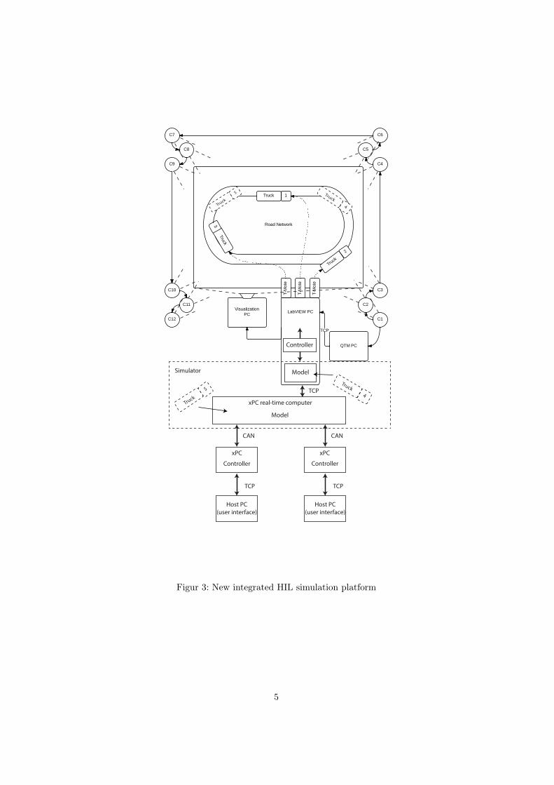
xPC

CAN

TCP

Host PC(user interface)

CAN

TCP

Host PC(user interface)

Simulator

Controller

xPC real-time computer

Controller

Controller

Model

Model

xPC

TCP

Truck

4Truck

5

Truck4

Truck

5

Figur 3: New integrated HIL simulation platform

5

Appendix B

Scania GCDC CAN Messages

Figure B.1: Simulink Block Sets for GCDC20 CAN Message

61

Figure B.2: Simulink Block Sets for GCDC00-07 CAN Messages

62

Appendix C

Data Packets

C.1 Main Program to Visualization tool

The following is structures of di↵erent data packets that are used in the system.

63

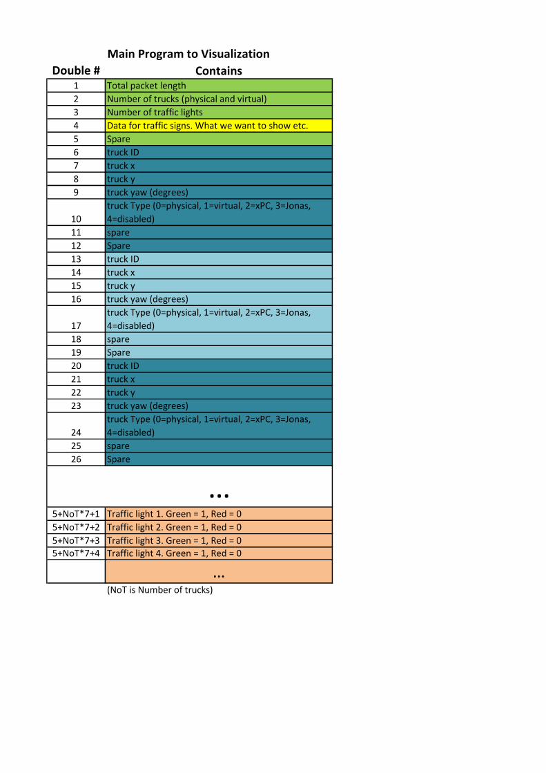
Main Program to Visualization

Double # Contains1 Total packet length

2 Number of trucks (physical and virtual)

3 Number of traffic lights

4 Data for traffic signs. What we want to show etc.

5 Spare

6 truck ID

7 truck x

8 truck y

9 truck yaw (degrees)

10

truck Type (0=physical, 1=virtual, 2=xPC, 3=Jonas,

4=disabled)

11 spare

12 Spare

13 truck ID

14 truck x

15 truck y

16 truck yaw (degrees)

17

truck Type (0=physical, 1=virtual, 2=xPC, 3=Jonas,

4=disabled)

18 spare

19 Spare

20 truck ID

21 truck x

22 truck y

23 truck yaw (degrees)

24

truck Type (0=physical, 1=virtual, 2=xPC, 3=Jonas,

4=disabled)

25 spare

26 Spare

…5+NoT*7+1 Traffic light 1. Green = 1, Red = 0

5+NoT*7+2 Traffic light 2. Green = 1, Red = 0

5+NoT*7+3 Traffic light 3. Green = 1, Red = 05+NoT*7+4 Traffic light 4. Green = 1, Red = 0

…(NoT is Number of trucks)

xPC to Main Program

Double # Contains1 x position [m]

2 y position [m]

3 yaw [Rad]

4 Velocity [m/s]

Main Program to xPC

Double # Contains1 Steering value (0:255)

2 Reference Speed [m/s]

xPC to xPC Monitor

Double # Contains1 Velocity [m/s]

2 Engine Speed [RPM]

3 Gear

4 Throttle

5 Brake

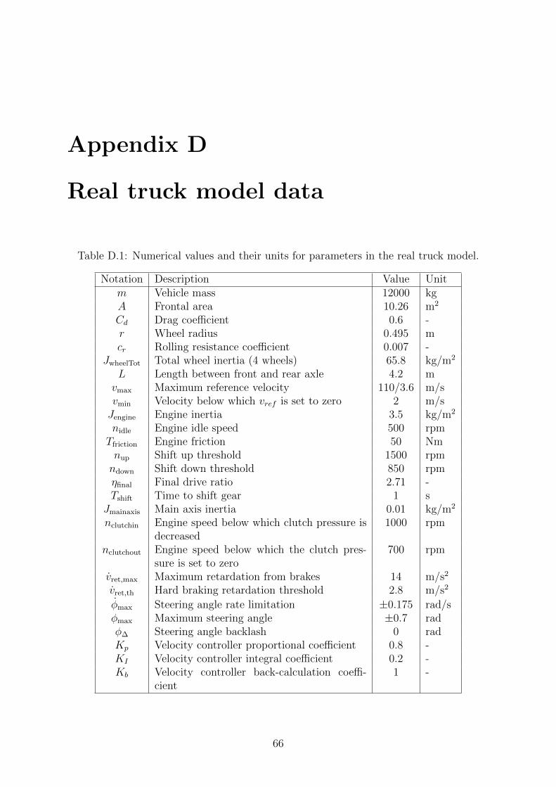
Appendix D

Real truck model data

Table D.1: Numerical values and their units for parameters in the real truck model.

Notation Description Value Unitm Vehicle mass 12000 kgA Frontal area 10.26 m2

C

d

Drag coe�cient 0.6 -r Wheel radius 0.495 mc

r

Rolling resistance coe�cient 0.007 -JwheelTot Total wheel inertia (4 wheels) 65.8 kg/m2

L Length between front and rear axle 4.2 mvmax Maximum reference velocity 110/3.6 m/svmin Velocity below which v

ref

is set to zero 2 m/sJengine Engine inertia 3.5 kg/m2

nidle Engine idle speed 500 rpmTfriction Engine friction 50 Nmnup Shift up threshold 1500 rpmndown Shift down threshold 850 rpm⌘final Final drive ratio 2.71 -Tshift Time to shift gear 1 s

Jmainaxis Main axis inertia 0.01 kg/m2

nclutchin Engine speed below which clutch pressure isdecreased

1000 rpm

nclutchout Engine speed below which the clutch pres-sure is set to zero

700 rpm

vret,max Maximum retardation from brakes 14 m/s2

vret,th Hard braking retardation threshold 2.8 m/s2

�max Steering angle rate limitation ±0.175 rad/s�max Maximum steering angle ±0.7 rad�� Steering angle backlash 0 radK

p

Velocity controller proportional coe�cient 0.8 -K

I

Velocity controller integral coe�cient 0.2 -K

b

Velocity controller back-calculation coe�-cient

1 -

66

Table D.2: The gear ratios, ⌘j

, used in the model.

j 1 2 3 4 5 6 7⌘

j

8.00 5.00 3.02 2.44 1.55 1.24 1.00

67