NASA-CR-199562

COMPUTATIONAL STRATEGIES FOR THREE-DIMENSIONAL FLOWSIMULATIONS ON DISTRIBUTED COMPUTER SYSTEMS f ( °l

Final Reportfor

NASA Grant NAG 2-869

Attn.: Dr. William Van DalsemNASA Ames Research Center

Moffett Field, CA 94035-1000

Prepared By

Lakshmi N. Sankar, ProfessorRichard A. Weed, Graduate Research Assistant

School of Aerospace EngineeringGeorgia Institute of Technology, Atlanta, GA 30332-0150

August 1995

XNIPG 95 00591) COMPUTATIONAL N96-13227STRATEGIES FOR THREE-DIMENSIONALFLOW SIMULATIONS ON DISTRIBUTEDCOMPUTER SYSTEMS Final Report Unclas(Georgia Inst. of Tech.) 190 p

G3/34 0073245

https://ntrs.nasa.gov/search.jsp?R=19960003218 2020-04-08T13:55:00+00:00Z

BACKGROUND

This research effort is directed towards an examination ofissues involved in porting large computational fluid dynamics codesin use within the industry to a distributed computing environment.This effort addresses strategies for implementing the distributedcomputing in a device independent fashion and load balancing. A flowsolver called TEAM presently in use at Lockheed AeronauticalSystems Company was acquired to start this effort.

SUMMARY OF WORK DONE

All the objectives of the research proposal submitted to NASAhave been accomplished. Specifically, the following tasks werecompleted.

1. Mr. Richard Weed, a graduate student working on this projectported the TEAM code to a number of distributed computingplatforms. These platforms include (a) a cluster of HP workstationslocated in the School of Aerospace Engineering at Georgia Tech, (b) Acluster of DEC Alpha Workstations in the Graphics visualization lablocated at Georgia Tech, (c) a cluster of SGI workstations located atNASA Ames Research Center, and (d) An IBM SP-2 system located atNASA Ames Research center. The public domain PVM software wasused to establish communications between the processors.

2. A number of communication strategies were implemented.Specifically, the manager-worker strategy and the worker-workerstrategy were tested. The manager-worker strategy was found to besimpler to implement, but required a large amount of managerworkstation memory. It was found to be inferior to the worker-worker strategy where worker processors directly exchangeinformation.

4. A variety of load balancing strategies were investigated.Specifically, the static load balancing, task queue balancing and theCrutchfield algorithm were coded and evaluated.

5. The classical explicit Runge-Kutta scheme in the TEAM solverwas replaced with an LU implicit scheme. The performance of theimplicit scheme on a distributed platform was compared to that ofthe baseline code. In most instances, the implicit scheme was foundto be superior to the explicit scheme.

6. The implicit TEAM-PVM solver was extensively validatedthrough studies of unsteady transonic flow over an F-5 wing,undergoing combined bending and torsional motion.

These investigations are documented in extensive detail in Mr.Richard Weed's Ph. D. dissertation. A copy of this dissertation isenclosed as an appendix. At this writing, this thesis is beingreviewed by a committee of 5 Georgia Tech faculty members, andminor changes to the dissertation are likely. A final draft of Mr.Weed's dissertation will all the corrections will be mailed to ourtechnical monitor, Dr. William Van Dalsem, in September 1995.

EXTERNAL INTERACTIONS AND TECHNOLOGY TRANSFER

The implicit PVM-TEAM code has been made available toresearchers at Lockheed Martin Corporation, and to researchers atWright Labs. The following papers were also published.

1. Weed, R. and Sankar, L N., "Computational Strategies for Three-Dimensional Flow Simulations on Distributed Computer Systems," AIAAPaper 94-2261.

2. Weed, R. and Sankar, L N., "Computational Strategies for Three-Dimensional Unsteady Flow Simulations on Distributed ComputingSystems," Proceedings of the NASA Computational AerosciencesWorkshop, March 7-9,1995.

PRECEDING PAGE BLANK WOT FILMED

ACKNOWLEDGMENTS

This work was supported by the NASA Ames Research Renterunder Grant NAG-2-869. The technical monitors were Dr. WiiliamVan Dalsem and Dr. Terry Hoist. The authors are thankful to Mr. FrankWitzeman of Wright Labs for providing the TEAM code and sampleinput deck for starting this effort. The present authors wish tothank Dr. Pradeep Raj and Mr. Brian Goble of Lockheed MartinCorporation for their assistance and encouragement throughout thiseffort. The authors are also thankful to Merritt Smith of NASA AmesResearch Center for valuable assistance on all aspects of thepresent research.

APPENDIX

COMPUTATIONAL STRATEGIES FOR THREE-DIMENSIONAL FLOW

SIMULATIONS ON DISTRIBUTED COMPUTING SYSTEMS

A Thesis

Presented to

The Academic Faculty

by

Richard Allen Weed

In Partial Fulfillment

of the Requirements for the Degree

Doctor of Philosophy in Aerospace Engineering

Georgia Institute of Technology

August 1995

COMPUTATIONAL STRATEGIES FOR THREE-DIMENSIONAL FLOW

SIMULATIONS ON DISTRIBUTED COMPUTING SYSTEMS

Approved:

Lakshmi N. Sankar, Chairman

Suresh Menon

Stephen M. Ruffin

Date Approved'.

ACKNOWLEDGMENTS

I would like to express my profound gratitude to my thesis advisor, Dr. L. N. Sankar,

whose advice and encouragement has made this effort possible. It has been a distinct honor

to have had Dr. Sankar as a teacher, colleague, and friend over the many years I have

known him.

I would also like to thank Dr. Suresh Menon and Dr. Stephen Ruffin serving on the

thesis advisory committee. In addition, I would also like to thank acknowledge die

contributions of Dr. P. K. Yeung and Dr. Karsten Schwann as members of the thesis

reading committee. Special thanks are due to the final member of the thesis reading

committee, Dr. Pradeep Raj, of the Lockheed Aeronautical Systems Company for his

many helpful suggestions and comments throughout the course of this work and for

providing access to the baseline computer code and computational grids used in this effort

This work was supported by the National Aeronautics and Space Administration under

grant number NAG 2-869.1 would like to express my appreciation to Dr. Terry Hoist and

Dr. Bill Van Dalsem at NASA's Ames Research Center who served as technical monitors

for the grant for providing both monetary support and access to the National Aerodynamics

Simulation facility's computer resources. In addition, I would like to express my gratitude

to Mr. Merritt Smith of the Computational Aerosciences Branch at NASA Ames and Dr.

Christopher Atwood of Overset Methods, Inc. for their helpful discussions and

suggestions during my work period at NASA Ames.

I would like to thank the Lockheed Aeronautical Systems Company for providing

support for tuition and books during the initial pan of my graduate career at Georgia Tech

and for providing me the opportunity to continue my studies while serving as a full-time

employee.

I would like to thank my former colleagues at Lockheed, Dr. George Shrewsbury, Dr.

Marilyn Smith, and Dr. David Schuster for their friendship and help in preparing for the

oral qualifying exam and Dr. Ashok Bangalore for our many discussions about distributed

computing. I would like to add a special thanks to Dr. Larry Birckelbaw and Mrs. Luly

Birckelbaw for the friendship and kindness they have shown me over the years and for

encouraging me to complete my degree requirements.

Finally, I would like to dedicate this work to my parents and express my profound

thanks for all the love and encouragement they have given me over the course of my life.

This work would not have been completed without their constant moral support I thank

them for all the sacrifices they have made to turn my dreams of becoming an engineer into a

reality.

rv

TABLE OF CONTENTS

ACKNOWLEDGMENTS Hi

TABLE OF CONTENTS v

LIST OF TABLES ix

LIST OF ILLUSTRATIONS x

NOMENCLATURE xii

SUMMARY xvi

L INTRODUCTION 1

1.1 Motivation for the Present Research 2

1.2 Survey of Literature on Parallel Processing and CFD 4

1.3 Overview of the Present Research 6

1.3.1 Objectives and Approach 6

1.3.2 The Three-Dimensional Euler//Navier Stokes Aerodynamic Method 8

1.4 Organization of the Dissertation 8

H. MATHEMATICAL FORMULATION OF THE EULER AND

NAVIER-STOKES EQUATIONS 10

2.1 Integral Form of the Governing Equations 10

2.2 Non-Dimensionalization of the Governing Equations 17

2.3 Reynolds Averaged Formulation for Turbulent Flow 19

2.4 The Governing Equations in General Coordinates 22

ffl. NUMERICAL FORMULATIONS OF THE EULER AND

NAVIER-STOKES EQUATION 25

3.1 Finite Volume Spatial Discretization Procedure 25

3.1.1 Calculation of Metric Quantities 28

3.1.2 Calculation of Inviscid Fluxes 30

3.1.3 Calculation of Viscous Fluxes 31

3.2 Artificial Dissipation Models 32

3.2.1 Standard Adaptive Dissipation 34

3.2.2 Modified Adaptive Dissipation 37

3.2.3 Flux-limited Adaptive Dissipation 37

3.2.4 Matrix Based Dissipation 39

3.3 Boundary Conditions 42

3.3.1 Far-Field Boundary Conditions 43

3.32 Solid Surface Boundary Conditions 44

3.3.3 Fluid and Symmetry Plane Boundary Conditions 46

3.4 Explicit Solution Procedure 49

3.4.1 Multi-Stage Time Stepping 49

3.4.2 Enthalpy Damping 51

3.4.3 Residual Smoothing 52

3.4.4 Local Time Stepping 53

3.5 Implicit Integration Procedure 54

3.5.1 Commonly Used Implicit Schemes 55

3.5.2 The LU-SGS Scheme 59

3.6 Moving Grid Procedures 64

VI

IV. DISTRIBUTED COMPUTING PROCEDURES AND

IMPLEMENTATION 67

4.1 The PVM Message Passing Interface 67

4.2 Communication Strategies 69

4.2.1 Communications Performance Factors 70

4.2.2 The Manager/Worker Strategy 72

4.2.3 The Worker/Worker Strategy 73

4.3 Load Balancing 73

4.3.1 Task Queue Load Balancing Procedure 77

4.3.2 The Modified Crutchfield Algorithm 78

4.4 Implementation of the Distributed Computing Modifications 81

4.4.1 Synopsis of Modifications to the Baseline Code 81

4.4.2 Boundary Update Procedure 82

V. STEADY FLOW SIMULATIONS ON NETWORK BASED

SYSTEMS 84

5.1 Validation and Performance of the Initial Distributed Solver 85

5.1.1 The MBB Body of Revolution No. 3 85

5.1.2 The ONERA M6 Wing 90

5.1.3 Lockheed/AFOSRWingC 97

5.2 Implementation and Validation of the Second Distributed Solver 103

52.1 Comparison of the Performance of the Load Balancing Procedures 103

522 Implementation of the Implicit Solver 106

VI. STEADY AND UNSTEADY SIMULATIONS ON THE NAS SP2 108

6.1 Wing C Euler Simulations 109

6.2 Wing C Viscous Simulations 114

vu

6.3 F5 Wing Simulations 119

6.3.1 F5 Wing Test Configuration 120

6.3.2 Computational Grid System 123

6.3.3 Results of Unsteady Simulations 125

6.3.3.1 Unsteady Euler Simulations 127

6.3.3.2 Unsteady Viscous Simulations 135

6.3.4 Steady Flow Results 138

VII. CONCLUSIONS AND RECOMMENDATIONS 143

7.1 Conclusions 144

7.2 Recommendations 146

APPENDIX A. THE BALDWIN-LOMAX TURBULENCE MODEL 148

APPENDIX B. THE INVISCID FLUX JACOBIAN MATRICES 152

APPENDIX C. MANAGER AND WORKER PSEUDO CODES 154

REFERENCES 158

VITA 168

vui

LIST OF TABLES

Table

5.1 Comparison of Computed ONERA M6 Loads and Convergence Parameters 95

6.1 Total Wing Load Coefficients and Convergence Data on Different Processors

for the Explicit and Implicit Solvers 112

6.2 Computed Load and Convergence Data for the Explicit and Implicit Schemes

After 1400 and 2000 Steps 114

6.3 Comparison of Total Loads and Convergence Data for the Viscous Wing C Case

Using the Explicit and Implicit Solvers 118

6.4 Span wise Locations of Experimental Pressure Data for the F5 Wing 121

IX

LIST OF ILLUSTRATIONS

Figure

3.1 Computational Cell 29

3.2 Decomposition of Tetrahedron 29

3.3 Class 2 and Class 3 Fluid Boundary Conditions 48

3.4 Oblique Sweep Planes for LU-SGS Scheme 63

4.1 The Manager/Worker Strategy 73

5.1 MBB Body and Symmetry Plane Grids 86

5.2 Baseline and Distributed Solver Convergence for the MBB Body 87

5.3 Correlation of Computed MBB Body Pressure Distributions with Experiment 88

5.4 MBB Body Turnaround Performance for the Baseline and Distributed Solver 89

5.5 ONERA M6 Wing Planform and Symmetry Plane Grids 91

5.6 Convergence Rates for ONERA M6 Wing with MAD Dissipation 92

5.7 ONERA M6 Convergence Rates with Increased MAD Dissipation Coefficients 93

5.8 The Effect of Lagging Zonal Boundary Updates with SAD Dissipation 94

5.9 ONERA M6 Wing Surface Pressure Distributions at 50% Span 96

5.10 ONERA M6 Wing Surface Pressure Distributions at 70% Span 97

5.11 Wing C Symmetry Plane Grid 98

5.12 Wing C Planform Grid 99

5.13 Wing CEuler Grid Zonal Point Distribution 100

5.14 Performance of the Ad Hoc and Task Queue Load Balancing Schemes 102

5.15 Comparison of Speedup for Static and Task Queue Balancing SGI Systems 104

5.16 Static and Task Queue Load Balance for Three Processors 105

5.17 Static and Task Queue Load Balances for Five Processors 106

6.1 Comparison of Turnaround Performance for the Explicit and Implicit Solvers 110

6.2 Comparison of Explicit and Implicit Scheme Speedups 111

6.3 Grid Point Distribution for the Viscous Wing C Grid 115

6.4 Load Balance for Viscous Grid with Five Processors 116

6.5 Convergence of Explicit and Implicit Schemes with Initial Dissipation Values 117

6.6 Convergence of Explicit and Implicit Schemes with Increased Dissipation 118

6.7 F5 Experimental Test Configuration (Reference 130) 120

6.8 F5 Wing Planform and Symmetry Plane Grids 124

6.9 Four Processor Real and Imaginary Pressure Distributions for the Inviscid F5

Wing Case, M=0.9, F=40Hz. 128

6.10 Comparison of 4,9, and 18 Processor Real and Imaginary Pressure Distributions

for the Inviscid F5 Wing Case, M=0.9,F=40Hz. 132

6.11 Comparison of Manager/Worker and Worker/Worker Performance 134

6.12 Comparison of Viscous and Inviscid Pressure Distributions for the F5 Wing

Using Four Processors, M=0.9, F=40Hz. 136

6.13 The Effect of Time Step Size on the Average Change in Density with Time for

the Steady F5 Wing Case Using the Implicit Solver, M=0.9 139

6.14 The Effect of Time Step Size on the L2 Norm of the Continuity Equation for

the Steady F5 Wing Case Using the Implicit Solver, M=0.9 140

6.15 The Effect of Time Step Size on the Number of Supersonic Points for

the Steady F5 Wing Case Using the Implicit Solver, M=0.9 140

6.16 Steady Viscous Pressure Distributions for the F5 Wing Case. 141

XI

NOMENCLATURE

A3.C flux Jacobian matrices

c speed of sound, chord length

CD total wing drag coefficient

CFL Courant-Friedrech-Lewy number

CL total wing lift coefficient

CM total wing moment coefficient

Cp pressure coefficient

cp specific heat at constant pressure

Cy specific heat at constant volume

D diagonal operator in LU-SGS scheme

D^Dn,D{ difference operators

d dissipative flux

E total energy

EjJ^, etc matrices in matrix dissipation formulation

e internal energy

F flux vector, frequency in Hertz

G non-convective flux

H total enthalpy

h enthalpy

IJ JC grid indices

xn

I identity matrix

J Jacobian of general coordinate transformation

k coefficient of thermal conductivity

L reference length

t turbulent length scale

M Mach number

n unit normal vector

p pressure

Pr Prandtl number

Q conservation variables

q velocity magnitude

R gas constant, Reimann invariants, residual

Re Reynolds number

r position vector

T temperature, elapsed time

t time

U contravariant velocity

u,v,w Cartesian velocity components

vs surface velocity

V cell volume

X,Y,Z Cartesian coordinates in inertia! system

x^z, grid speeds

a angle of attack, dissipation eigenvalue factor

xui

dissipation factor

ratio of specific heats

increment, forward difference operator

backwards difference operator, gradient operator

central difference operator

curvilinear coordinates

62,64 dissipation coefficients

X bulk viscosity coefficient

X( A), etc eigenvalue of the flux Jacobian matrices

6 mode shape, temporal accuracy parameter

K reduced frequency

A dissipation factor

\L molecular viscosity

Hx eddy viscosity

p density

p(A) spectral radius of flux Jacobian matrices

t shear stress

t^ etc components of stress tensor

xiv

O viscous dissipation function

0) vorticity

Superscripts

n time level

k integration stage

Subscrits

grid indices

E effective value

T turbulent quantity

t derivative with respect to time

x,y,z derivative with respect to the Cartesian coordinates

derivatives with respect to curvilinear coordinates

freestream quantity

xv

SUMMARY

In the present research, the issues involved in the development and implementation of

three-dimensional Computational Fluid Dynamics analysis methods on distributed parallel

computing systems are explored The growing requirements in the aerospace industry for

more cost effective aerodynamic simulations has led to research into the use of distributed

systems based on loosely and tightly coupled systems of engineering workstations as

substitutes for large scale supercomputer systems for large scale aerodynamic simulations.

However, effective computational strategies for implementing three-dimensional multi-zone

flow solvers on workstation based distributed systems are required to ensure that the

distributed parallel flow solvers provide the required levels of performance. In addition, die

effects of various computational procedures on die accuracy of both steady and unsteady

flow simulations must be evaluated. Finally, efficient procedures for implementing a

distributed parallel flow solver on a variety of distributed system needs to be quantified.

This research attempts to evaluate and define the most appropriate strategies for

implementing a cost effective distributed parallel flow solver for both steady and unsteady

flow simulations.

The approach taken in this research was to use an existing industry standard three-

dimensional multi-zone flow solver in conjunction with the Parallel Virtual Machine

software interface to develop a distributed parallel flow solver that was used to define and

evaluate efficient communications and load balancing strategies for workstation based

systems. The research was performed in two phases. In the first phase, an explicit flow

solver was implemented on small Ethernet based networks of engineering workstations.

Steady flow simulations for standard wing and body of revolution geometries were used to

xvi

evaluate a Manager/Worker communications strategy and two static load balancing schemes

The results of these simulations also demonstrated the effects of the zonal boundary

condition update procedures and numerical dissipation models on the accuracy and

convergence of the distributed flow solver. It was found that increased levels of dissipation

were required to maintain the convergence of die distributed solver. The adverse effects of

system load and communications overhead were demonstrated.

In the second phase of the research, an improved version of the baseline code was used

to develop both explicit and implicit flow solvers mat were implemented on the large scale

IBM SP2 distributed system at the NASA Ames Research Center. These solvers were

validated for both Euler and Navier-Stokes simulations using a standard test case. The

accuracy and performance the explicit and implicit distributed flow solvers were evaluated.

A series of unsteady flow analyses were performed using the implicit flow solver to

quantify the effect of the domain decomposition procedure used in the distributed solver on

solution accuracy. The test case for these simulations was the modal vibration of the F5

wing oscillating in pitch. The results of these tests led to the implementation and evaluation

of a second communications strategy that demonstrated improved performance for

increasing numbers of processors on the SP2 system. These results demonstrated the

viability of a distributed flow solver for unsteady flow simulations on a large scale

distributed system such as the SP2.

Finally, the utility of workstation based distributed flow solvers for real world

aerodynamic analyses of both steady and unsteady flows was demonstrated. The

distributed flow solvers developed in this research are felt to provide the basis for a

production aerodynamic analyses and design tool

jcvu

CHAPTER I

INTRODUCTION

During the past decade, an increasing amount of research activity in Computational

Fluid Dynamics (CFD) has been devoted to harnessing the power of parallel computing

architectures to improve the total throughput of CFD codes. This effort was prompted by

several factors. Existing vector supercomputers such as the CRAY systems are

approaching the theoretical limit in processing speed obtainable by a single processor. In

the same period of time, higher order CFD methods such as flow solvers based on

numerical solution of the Euler or Navier-Stokes equations have obtained a wider

acceptance in the aerospace community as viable tools for aerodynamic design and

analysis. Current production CFD codes in use in the aerospace industry are capable of

performing both Euler and Navier-Stokes analyses on complete aircraft [1,2,3]. However,

these types of analyses are expensive in both time and money even for current large scale

supercomputing systems. This has led to increasing emphasis on reducing the overall costs

and increasing the throughput of CFD analyses in order to integrate them into the overall

design process. In addition, research is underway to develop multi-disciplinary tools that

combine structural analyses, aerodynamic analyses, and optimization procedures into a

single analyses method. These multidisciplinary methods require computing power that is

beyond the performance capabilities of a single processor. The increased demand for faster

throughput and increasing problem size has led to research in the use of parallel processing

systems for CFD simulations.

1.1 Motivation For The Present Research

All parallel computing systems utilize multiple processors of varying levels of power

and sophistication to achieve performance improvements over serial computers. Parallel

systems can be differentiated by the relationship of the memory subsystem to individual

processors and the number of data streams available on the system [4]. Memory

subsystems are classified as either distributed memory or shared memory. On distributed

memory systems, each processor has direct access to only its own local memory space.

Access to information on the other processors is accomplished by passing data messages or

packets over a high speed communications network. On shared memory multiprocessors,

each processor accesses the same global memory space.

Over the last few years, the Multiple Instruction-Multiple Data (MIMD) systems such as

the Cray Y-MP, Cray C-90, and the Intel Paragon and iPSC/860 systems have supplanted

the Single Instruction-Multiple Data (SIMD) shared memory machines such as the

Connection Machine as the predominant parallel systems for CFD calculations. The Cray

systems are examples of shared memory machines while the Intel systems use distributed

memory. Shared memory machines are best suited for problems that require fine grain

parallelism where work is distributed among the processors at the level of individual loops

or vectors. Distributed memory machines are best suited for problems that can utilize coarse

grain parallelism where a large problem can be decomposed into smaller problems or tasks

that are mapped to the individual processors.

In the mid 1980's, studies performed by Johnson [5] and Gropp and Smith [6] pointed

out the advantages and disadvantages associated with the use of parallel processing systems

2

for GFD simulations. In particular, the performance penalties due to communications

overhead between processors and the necessity of maintaining an equal balance of work

among processors was emphasized. In addition, the problems associated with transferring

existing serial algorithms to the parallel environment were described Therefore, a

significant amount of research has centered on developing new algorithms to take

advantage of the task level parallelism inherent in the numerical solutions of the Euler and

Navier-Stokes equations and the problems associated with porting existing algorithms to

different parallel architectures. Most of this research has been targeted at massively parallel

architectures that are composed of large numbers of simple processors such as the

Connection Machine CM-2 and CM-5 and the CRAY T3D systems which can utilize

thousands of processors, smaller distributed multi-processor versions of vector machines

such as the CRAY C-90 which have typically four to eight specialized high-speed

processors, and large distributed multi-processor systems such as the Intel Paragon and

iPSC/860. However, the difficulties in porting existing codes to these systems along with

their high acquisition and overhead costs and limited availability have prevented their wide

spread use by the aerospace industry. The rapid development of high-speed engineering

workstations has led to large distributed systems such as die IBM SP2 system [7] based on

existing workstation processors.

Recently, the increasing performance to price ratios and availability of engineering

workstations have led some researchers to explore the viability of linking clusters of

workstations together to form distributed parallel systems [8]. This interest was also

prompted by the fact that most engineering workstations are idle during off hours and

represent an underutilized computing resource of enormous potential. In addition, the

recent development of standardized application programming interfaces such as the Parallel

Virtual Machine (PVM) system [9,10,11,12] have greatly reduced the effort required to

link together workstations into a distributed parallel system. The recent work of Smith and

3

Palas [13] demonstrated the feasibility of a PVM based parallel distributed flow solver.

They pointed out the need for effective computational procedures tailored to workstation

based distributed systems. This research was undertaken to help define these procedures

and to evaluate the effort required to implement an existing flow solver as a parallel solver

on distributed systems using PVM. In addition, the present research was undertaken to

determine the viability of a PVM based multi-zone parallel flow solver for unsteady flow

simulations

1.2 Survey Of Literature On Parallel Processing And CFD

In the 1980's, early attempts to employ parallel processing in CFD centered on the

development of fine grain solution algorithms for the Euler and Navier-Stokes equations

that allowed inner loops in the solver to be processed in parallel. The multitasking approach

used on Cray computing systems is an example of loop level parallelism. An example of

the effectiveness of multitasking for CFD calculations is given in the work of Swisshelm

et al. [14]. Other authors such as Patel, Sturek, and Jordan [15] developed parallel

solution algorithms for multiprocessor MIMD systems such as the Denelcor HEP

computers. As the decade progressed, parallel algorithm development was focused on data

parallel SIMD systems such as the Connection Machine CM2 and large multiprocessor

MIMD systems such as the Intel iPSC/860 systems.

In 1989, several researchers presented results for Euler and Navier-Stokes calculations

on the Connection Machines. Wake and Eglof [16] ported a hybrid implicit-explicit Navier-

Stokes solver for helicopter rotor analysis to the CM-2 and achieved performance that was

slightly better than on a single processor Cray-2 system. An improved version of the code

[17] was able to achieve twice the performance of a Cray 2 system. Long, Khan, and

Sharp [18] implemented an three-dimensional explicit Euler/Navier-Stokes solver on the

4

CM-2 using the Lisp programming language. Another implementation of a Navier-Stokes

solver on the CM-2 was described by Agarwal [19]. Kallinderis and Vidwans [20] have

introduced a generic parallel adaptive-grid Navier-Stokes solver that has executed

successfully on both the CM-2 and Cray Y-MP/8 systems. These flow solvers were based

on structured grid systems. Hammond and Earth [21] developed an unstructured Euler

solver for the CM-2. Morano and Mavriplis [22] have also implemented an unstructured

Euler solver on the CM-5 machine operating in MIMD mode.

The introduction of large distributed parallel systems such as the Intel iPSC/860 has led

to a significant amount of research for these types of machines. Ryan and Weeratunga [23]

used a distributed parallel version of an overset grid flow solver to compute Navier-Stokes

flowfields for supersonic vehicles on the iPSC/860. Hixon and Sankar [24] used domain

decomposition and an implicit flow solver to perform unsteady two-dimensional flow

calculations. Otto [25] used the iPSC/860 to perform Navier-Stokes calculations of

chemically reacting flows. Das et al. [26] and Venkatakrishnan et aL [27,28] have

developed parallel flow solvers for unstructured grid systems using the iPSC/860.

Unsteady aeroelastic flow simulations have been performed by Promono and Weeratunga

[29] and Byun and Guraswamy [30] using the iPSC/860 and Paragon systems. Imlay and

Soetrisno [31] studied the problems of porting implicit flow solvers for chemically reacting

flows to both shared and distributed memory MIMD machines. Fatoohi [32] has described

the effort required to adapt the NASA Ames INS3D flow solver to three different parallel

systems.

In the past two years, research in the area of workstation based distributed systems has

grown due to the increasing pressure of budget constraints in the aerospace industry and

the introduction of software such as PVM. The previously cited work of Smith and Palas

[13] proved the viability of a workstation based system for real world applications. This

has led to a wide range of workstation based programs for distributed systems. An

5

overview of these programs was given in Reference 33. Hayden, Jayasimha, and Pillay

[34] compared the performance of a workstation based system with other shared and

distributed memory systems. Deshpande, Feng, and Merkle [35] studied the effect of

various network communications protocols on the performance of a parallel flow solver on

a distributed network system. The majority of the distributed flow solvers have been

applied to steady-flow only. Recently, Bangalore et aL [36,37] used a workstation based

distributed system to simulate the unsteady viscous flow over rotor systems. Finally, the

first phase of the present research was reported in References [38] and [39].

1.3 Overview of the Present Research

1.3.1 Objectives and Approach

The main objectives of this research are to evaluate the issues involved in porting, fine

tuning, and improving an existing flow solver for optimal performance on a distributed

parallel system. The research emphasizes the development and evaluation of efficient

computational strategies for both steady and unsteady flow. The approach taken was to

utilize an existing multi-zone solver, the Lockheed/AFOSR Three-Dimensional

Euler/Navier-Stokes Aerodynamic Method (TEAM) code [40], and the PVM software

interface to develop a parallel distributed flow solver that could run on a variety of

hardware platforms.

A variety of multi-zone solvers have been developed in the past decade [41,42,43].

The common feature of all these flow solvers is that they break the computational domain

into several different grids with either abutting or overlapping interfaces. This natural

domain decomposition makes multi-zone solvers such ideally suited for distributed

computing systems because each zone or a set of zones can be mapped to separate

processors. The solution in each zone is generated concurrently using the same solution

algorithm running on each processor. Therefore, a parallel flow solver can be implemented

with relatively minor code modifications. However, die performance of a distributed flow

solver can be severely impacted by the communications overhead introduced by the size

and number of messages that are exchanged during the solution process to synchronize the

solution and transfer zonal boundary information. Therefore, effective communications

strategies must be implemented to reduce the overhead and maintain system performance.

In addition, efficient procedures are required to maintain as closely as possible an equal

level of work on each processor. This reduces the amount of time each processor is idle

during the solution cycle. This process is called load balancing.

The present research was performed in two phases. In the first phase, a version of the

Lockheed/AFOSR TEAM code was obtained from the U.S. Air Force to serve as a baseline

code. Version 3.1.5 of PVM was installed on a system of four Hewlett-Packard

workstations on an Ethernet based network. The PVM software interface was used to

implement a distributed version of the baseline code (PVMTEAM) that was used as a test

bed for evaluating code performance and implementation issues. Standard test cases were

used to evaluate overall performance and the effects of such issues as boundary update

procedures and the effects of numerical dissipation on the solver performance and

accuracy. The code was also run on a network of Digital Equipment Company (DEC)

ALPHA workstations. In the second phase, an improved version of the code was

implemented on a system of Silicon Graphics Co. (SGI) workstations. This code was later

ported to the IBM SP2 distributed supercomputer system at NASA Ames Research center.

The improved code was used to evaluate two different load balancing algorithms and two

communications strategies. Finally, this version of the code was used to perform a series of

unsteady flow simulations for an oscillating wing.

1.3.2 The Three-Dimensional Euler/Navier-Stokes Aerodynamic Method

The baseline code was developed by the Lockheed Aeronautical Systems Company for

the United States Air Force. This code is a multi-zone explicit finite volume code based on

the mulit-stage Runge-Kutta time stepping scheme of Jameson et al. [44]. Acceleration

techniques such as residual smoothing and enthalpy damping are employed to extend the

stability bounds of the explicit scheme and allow the use of larger Courant numbers. The

code has been validated for a wide variety of geometries and flow conditions. The multi-

zone formulation allows the code to be applied to complex geometries such as complete

aircraft The code has a wide variety of boundary condition options for both external and

internal flows. In addition, several numerical dissipation models are available that insure

stable solutions over a wide range of Mach numbers. The code employs a dynamic memory

allocation scheme that sizes solution arrays at run time. This eliminates the need to

recompile the code whenever the size of the grid systems change. These features made the

TEAM code an excellent baseline for the present research.

1.4 Organization Of The Dissertation

The remaining chapters of this dissertation are organized in the following manner. A

discussion of the mathematical formulation of the conservation law form of the governing

equations is given in Chapter 2. The numerical algorithms used in the distributed flow

solver is described in Chapter 3. This includes complete discussions of the spatial

discretization techniques, dissipation models, boundary conditions and time stepping

schemes used in die research. Chapter 4 summarizes the procedures used to implement the

distributed version of the solver. This includes discussions of the communications and load

balancing strategies used in the code. Results for both steady and unsteady flow

simulations on the workstation based systems used in this research are presented in Chapter

8

5. The results of steady and unsteady simulations on the IBM SP2 system at NASA's

Numerical Aerodynamics Simulation (NAS) facility are presented in Chapter 6. The final

conclusions and suggestions for future results are presented in Chapter 7.

CHAPTER H

MATHEMATICAL FORMULATION OF THE EULER AND

NAVIER-STOKES EQUATIONS

This chapter will discuss the formulation of the Reynolds-Averaged Navier-Stokes

equations used in the baseline Three-Dimensional Euler/Navier-Stokes Aerodynamic

Method code. The Euler equations will be discussed as a subset of the Navier-Stokes

equations. The procedure used to non-dimensionilize the Euler and Navier-Stokes

equations will be described. The turbulence model and procedures used to compute the

thermodynamic and transport properties required to provide closed systems of equations

will also be discussed

2.1 Integral Form of The Governing Equations

The formulation of the Navier-Stokes Equations used in the baseline code is derived

from the integral form of the equations obtained by application of Reynolds Transport

Theorem [45] and the principles of conservation of mass, momentum, and energy to a

control volume of arbitrary shape surrounding a cell of fluid moving in space and time.

Following Vinokur [46], a general conservation law for a fluid cell of volume V(t) moving

through a finite region of space over a finite interval of time, tz- tj, can be written as

10

J QdV- J QdV + J1' $F»ndSdt = 0 (2.1)v<t,) V(t,) '' S(t)

where Q is a vector of conserved variables per unit volume, F is the flux of Q per unit

volume per unit time, S(t) is the surface bounding the volume, dS is a differential element

of S, and n is a outward pointing unit vector normal to dS. The flux F can be written as

F = (u-vs)Q + G (2.2)

where u is the fluid velocity vector and vs is the velocity of the surface element dS. The first

term in Equation (2.2) represents the convective component of the flux and the quantity G

is the non-convective component of the flux due to forces acting on the volume and the

dissipation and transfer of energy into and out of the volume. For the Euler and Navier-

Stokes equations, the flux terms arise from the fluid pressure acting on the surface, shear

stresses due to viscosity, and heat transfer across the cell surface. If all the variables are

assumed to be continuous in time, Equation (2.1) can be written in the more familiar

integro-differential form

(2.3)

For the compressible Euler and Navier-Stokes equations, the conserved variables are

normally taken to the density p, the fluid momentum pu, and the total energy per unit

volume E. The vector Q can be written as

11

Q=(p,pu,pv,pw,E)T (2.4)

where u, v, and w are the Cartesian components of the fluid velocity with respect to an

interial coordinate system. The convective component of the flux F can be expanded into

its Cartesian components and combined with the pressure force and work contributions

from G to give the inviscid flux components Fx, FY, and Fz which can be written as

Fv =

P(u-xt)

pu(u-x t) + p

pv(u-xt)

pw(w-x t);FY =

P(v-yt)pu(v-y t)

pv(v-yt) + p

pw(v-y,)

lH(v-y t:

p(w-zt)

pu(w-z t)

pv(w-zt)

pw(w-z,) + p(2.5)

where x,, yt, andz, are the Cartesian components of cell surface velocity with respect to

an inertial coordinate system and p is the static pressure. The system of equations formed

by substituting the inviscid components of F and the conserved variables defined in

Equation (2.4) into Equations (2.1) and (2.3) comprise the Euler Equations.

The Navier-Stokes equations are obtained by including the forces due to viscous

stresses into the momentum equation components of the flux and the energy transfer into

and out of the control volume due to thermal conduction and the dissipation due to the

deformation of the volume by viscous stresses into the energy equation. The Cartesian

components of the flux due to viscous stresses and heat transfer F^, Fyy, and F^ can be

defined as

12

( o ^ ( o ^ ( o >

3Tdx

and the viscous stress and dissipation terms are defined as

dv-+

.du dv.

.dv dw.

+ VTYY

(2.6)

(2.7a)

(2.7b)

(2.7c)

(2.7d)

(2.7e)

(2.7f)

(2.7g)

(2.7h)

13

where k is the coefficient of thermal conductivity, T is the temperature, jo. is the coefficient

of molecular viscosity and X is the bulk viscosity coefficient The bulk viscosity X can be

related to the molecular viscosity \i by Stokes hypothesis

X = -|n (2.8)

The viscous stress and heat flux terms can be be replaced by "thin-layer"

approximations that are analogous to the classical boundary layer approximations. The thin-

layer approximation is obtained by excluding derivatives of the flow quantities along

specified directions. For flows bounded by a solid surface, these directions are usaully

taken to be the streamwise coordinates approximately tangent to the surface. Only the

derivatives along the coordinate approximately normal to the surface are retained. This

approximation has proven to provide a sufficiently accurate simulation of the viscous flux

for a wide range of flows.

Closure of the preceding system of equations requires definitions for the

thermodynamic variables (p, p, T, E) and the transport properties Qi, k). Analytical

relationships between these variables are also required. Pressure can be related to density

and temperature through the equation of state for a perfect gas*

p = pRT (2.9)

where R is the gas constant The specific internal energy e, the specific enthalpy h, and the

ratio of specifics heats y can be defined as

14

e = c¥T ; h = cpT ; y = -t (2.10)

where Cy is the specific heat at constant volume and cp is the specific heat at constant

pressure. Pressure and temperature can be related to internal energy by using Equations

(2.9) and (2.10) and the following definitions for die specific heats

This leads to relationships for pressure and temperature of the form

p = (y-l)pe ; T = ̂ L^ (2.12)X.

The specific heats cv and cp are constants when the gas is both thermally and calorically

perfect. Under the assumption of a thermally and calorically perfect gas, the ratio of

specific heats for air at standard conditions has a value of 1.4. For imperfect gases, die

thermodynamic properties must be computed from tables or curve fits or die system of

equations must be modified to solve for die constituent species of die gas [47]. The final

thermodynamic relationship is die definition of die total energy per unit volume E which is

given by

15

u2 + v2 + w2

= p(e+U * V * W ) (2.13)

The coefficient of molecular viscosity \i has been shown empirically to be a function of

temperature for most gases over the range of temperatures where perfect gas assumptions

are valid. The most commonly used relationship for viscosity is Sutherland's law [48]

which is given by

where C, and C2 are constants for a given gas. The coefficient of thermal conductivity can

be appoxmated by the relation given by Worsoe-Schmidt and Leppeit [49]

k = Ta71 (2.15)

However, it is often more convenient to determine k from the definition of the Prandtl

number Pr

(2.16)

The Prandtl number is approximately constant for most gases and has a value of 0.72 for

air at standard conditions.

The preceding systems of equations define the general time-dependent or unsteady

Euler and Navier-Stokes equations for a compressible fluid in conservation law form. This

16

form of the equations is favored over non-conservative formulations because of its ability

to maintain global conservation throughout the fluid space even when discontinuities such

as shock waves are present In practice, die dimensional variables in the governing

equations are recast as non-dimensional variables to remove any dependency on a particular

set of units of dimension from the equations. For practical calculations of turbulent flows,

additional modifications must be made to the system to account for the random fluctuations

in the flow variables induced by turbulence. These modifications are described in sections

2.2 and 2.3 of this chapter.

2.2 Non-Dimensionalization of the Governing Equations

Non-dimensional forms of the flow variables in the governing equations are obtained

by dividing dimensional quantities such as density and velocity by an appropriate set of

reference values. These reference values are normally taken to be the values of the free-

stream at infinity. The set of non-dimensional variables used in the baseline code [40] are

defined as follows

-,E=^=- (2.17a)P. " c- " c. " c. p.

P ~fT ' " T L ' ^ ' i L * "kT'1

(2.17c)

17

where a bar denotes a dimensional quantity. The variable L is a characteristic length such as

wing root chord and c. is the free-stream speed of sound given by

(2.18)

Substitution of the non-dimensional variables in the governing equations leads to two

additional non-dimensional quantities, the Reynolds number Re and the Mach number M,

which are defined at the free-stream by the relations

.q.L M _ q.——, M.. - —». c.

(2.19)

where q. is the magnitude of the freestream velocity vector. For viscous flows,

Sutherland's law for molecular viscosity becomes

T.T5.

(2.20)

where the non-dimensional temperature is given by the non-dimensional equation of state

as T=p/p and Ts is a reference temperature which has a value of 110.4 °K for air.

18

The non-dimensional form of the conserved variables and the inviscid flux components

are unchanged from their dimensional forms. The viscous flux components retain their

dimensional form with the addition of a scale factor equal to VTM- / Re. , i.e. Equation

(2.6) become

VX.Y.Z

where F is the dimensional form of the viscous flux.

2.3 Reynolds Averaged Formulation for Turbulent Flow

Turbulent flow is characterized by random momentum and energy exchanges over a

broad spectrum of length and time scales [50]. Therefore, direct simulation of turbulent

flows using finite difference, finite volume, or finite element discretizations of the Navier-

Stokes equations would require extremely large numbers of computational points and

prohibitively small time steps to resolve all of the characteristic scales of the flow. In

addition, the random nature of the velocity fluctuations that are inherent in turbulent flows

must be treated statistically. Reynolds employed a simple decomposition of the flow

variables into time averaged values with a mean component and a fluctuating component

with zero mean over time [50]. This decomposition can be written as

(2.22)

19

where the primes represent the fluctuating values. When this averaging process is applied

to the Navier-Stokes equations, new terms appear in the equations that are functions of the

fluctuating components of velocity. In particular, momentum transfer terms are generated

that can be thought of as stresses. These terms are commonly called the Reynolds's

stresses. It is convenient to combine the additional terms generated by the fluctuating values

with the flux vectors based on the mean values. For example,

(2.23)

where FX can be written in terms of the fluctuating time averaged velocity components as

0

-puV

-pu'w'(2.24)

The Bossinesq assumption [51] is used to relate the Reynolds stresses to the mean strain

rates by means of a proportionality factor commonly referred to as the eddy viscosity. For

example,

(2.25)

20

The Bossinesq assumption allows the molecular viscosity and thermal conductivity to be

replaced by effective values defined in non-dimensional form as

(2.26)

where PrT is the turbulent Prandtl number which has an approximate value of 0.9 for air.

Closure of the Reynolds averaged Navier-Stokes equations requires a model for

evaluating the eddy viscosity jx,.. Several models of varying degree of accuracy and

complexity have been developed over the years to compute the eddy viscosity. The most

widely used models are the simple algebraic or zero-equation models of Cebeci and Smith

[52] and Baldwin and Lomax [S3]. The Baldwin-Lomax model has become the de facto

standard model for most engineering calculations. These models give acceptable

engineering approximations for attached flows or flows with moderate amounts of

separation. Models of this type are based on PrandtTs mixing length theory [51] which

relates the eddy viscosity to an appropriate length scale and characteristic turbulent velocity.

In the algebraic models, these values are computed from empirically defined relations.

Higher order models have been developed that use ordinary or partial differential equations

to compute the appropriate quantities. Examples of these are the one equation models of

Johnson and King [54] and Spalart and Allmaris [55] and the two equation Jones-Launder

k-e model [56]. The Baldwin-Lomax model has been used exclusively in the research. A

detailed description of the model is given in Appendix A.

21

2.4 The Governing Equations in General Coordinates

For arbitrary geometries, the solution of the Euler or Navier-Stokes equations is

normally performed in general curvilinear coordinate systems. This allows irregular

boundaries such as the curved surfaces of wings and fuselages to be mapped to align with

one or more of the curvilinear coordinates. For the differential forms of the governing

equations, a general coordinate transformation must be applied to the equations to map the

Cartesian system into the curvilinear system [51]. The partial derivatives in the Cartesian

system are recast in terms of partial derivatives in the curvilinear system scaled by

appropriate transformation metrics by means of the chain rule for differentiation. In

contrast, the integral formulations of Equations (2.1) and (2.3) can be applied directly in a

curvilinear system. All that is required is a consistent procedure for defining the cell face

areas, cell face unit normal and tangential vectors, and cell volumes. For both the integral

and differential forms of the governing equations, the inviscid flux normal to a cell face

with area ISI is given by

TJ _

P(UB-Vn)

puOJ.-Vpv(UB-V I S I (2.27)

where

UB = un, +vn, + wn,, VD = x.n, + y,n, (2.28)

22

This is equivalent to the inviscid flux in a set of general curvilinear coordinates (£,tl,0

when the metric quantities required in the general coordinate transformation are defined

geometrically as

k as*•* *» • • (2.29)

where k is one of the curvilinear coordinates £, TJ, or £, the quantities S^, SkY, and S^ are

the components of the area vector of a surface in the curvilinear system of where k is

constant, and V is the cell volume. The parameters k,, k,, and k, are equivalent to the

partial derivatives of the curvilinear coordinates with respect to the Cartesian system.

Substitution of these metrics into Equations (2.27) yields the inviscid flux in the curvilinear

system through a cell face. For example, the inviscid flux through a face where £ is

constant can be written as

pU

pwU + p^

(2.30)

where U = £xu + £,v+£Ew + £t is the contravariant velocity, J =1/V is the Jacobian of the

general coordinate transformation, and H=(E+p)/p is the total enthalpy. Therefore, the

23

evaluation of the integral form of the governing equations on a cell volume in a curvilinear

system is equivalent to die differential form in general coordinates when metric quantites

are defined consistently. Similar relationships exit for the other coordinate directions. The

viscous flux through £ can be written

The differential form of the governing equations in general curvilinear coordinates can then

be written as

dL,

where Q = Q/J and G, H, G v, and Hv are inviscid and viscous flux vectors in the T] and

analogous to Equations 2.31 and 2.32.

24

CHAPTER HI

NUMERICAL FORMULATIONS OF THE EULER AND

NAVIER-STOKES EQUATIONS

This chapter describes the numerical discretization of the governing equations by the

finite volume method used in the baseline and distributed flow solvers. The spatial

discretization procedures for the Euler and Navier-Stokes equations are presented along

with the methods used to compute metric quantities. The artificial dissipation models

required to stabilize the numerical schemes are discussed. The implementation of the

numerical boundary conditions is described. The explicit and implicit integration

methods used to solve the governing equations are presented for both steady and

unsteady flow. Finally, the special modifications required for unsteady analyses on

moving grid systems are given.

3.1 Finite Volume Spatial Discr^iyp^ion Procedure

In the finite volume method, the computational domain is subdivided into a grid of

discrete volumes or cells. The integral forms of the governing equations given by

Equations (2.1) and (2.3) are applied locally to each discrete volume. This leads to semi-

discrete numerical schemes in which the spatial and temporal terms can be uncoupled in a

manner similar to the classical Method of Lines [44] and evaluated by different methods.

25

Finite volume schemes are classified as "cell-centered" schemes if the flow variables

are defined at some point in the cell as a volumetric average of the variables over the cell

and "cell-vertex" schemes if the flow variables are defined at the vertices of the cell [57].

In three-dimensional structured grid systems, the volumes are hexahedrons. In

unstructured grid systems, the volumes are usually tetrahedral elements similar to those

used in finite element formulations [58]. For both classes of finite volume schemes, the

vertices of the volume are defined by their Cartesian coordinates. This eliminates the

need to specify a global coordinate transformation for curvilinear mesh systems. The

connections between the vertices that define the edges of the volume are normally taken

to be straight lines. Therefore, metric quantities such as cell volume and the areas and

normal vectors of cell faces can be computed using geometric relations [46]. The finite

volume scheme used in the baseline code is the structured cell-centered scheme

introduced by Jameson, Schmidt, and Turkel [44].

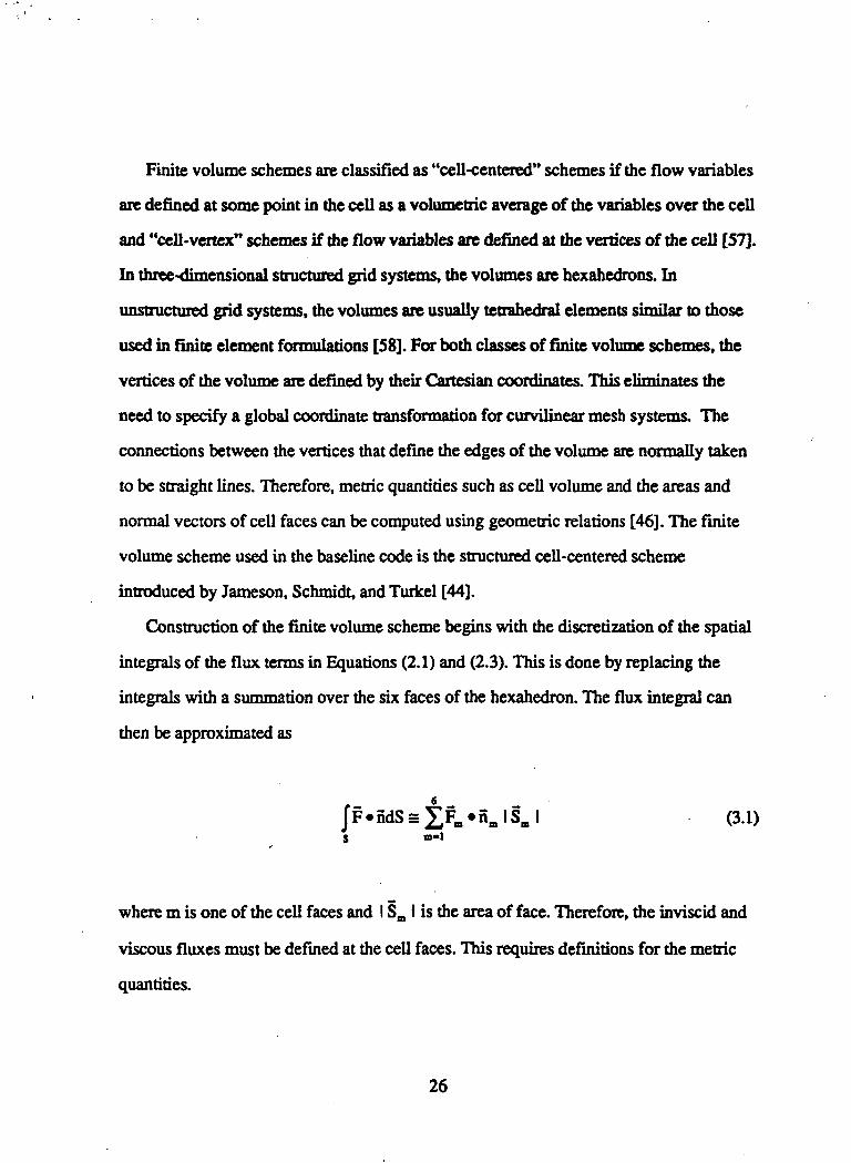
Construction of the finite volume scheme begins with the discretization of the spatial

integrals of the flux terms in Equations (2.1) and (2.3). This is done by replacing the

integrals with a summation over the six faces of the hexahedron. The flux integral can

then be approximated as

6 _

m-1

where m is one of the cell faces and I Sm I is the area of face. Therefore, the inviscid and

viscous fluxes must be defined at the cell faces. This requires definitions for the metric

quantities.

26

The volume integrals in Equation (2.1) are evaluated as the product of the average

value of the conserved variables in the cell and the cell volume. Therefore, the volume

integral at time t2 for a cell denoted by subscript J becomes

/QdV = QjY,|4 (3-2)V(t,>

To be consistent with the procedures used to compute the surface flux, it is more

convenient to interpret Q, as a value defined at some average point in the cell This

removes the exact equality implied by Equation (3.2) and makes the relation

approximate. For simplicity, the average point is taken to be the cell center defined by the

average of the position vectors of the cell vertices.

The time integral of the flux over each face m in Equation (3.1) can be approximated

by

(3.3)

where At = tj-tj , FB is the flux normal to the cell face, and 6 is a parameter used to define

the type of time integration scheme used. Values of 0 greater than zero yield implicit

integration schemes and a value of zero yields an explicit scheme. For implicit schemes,

the value of the flux at t2 is not known and must be linearized about the previous time

level t ,. Replacing t2 and t, with the level indices n and n+1 the discretized form of

Equation (2.1) becomes

27

6

m-1(QVT1 -(QV)° + At£((l-e)I? + 0*:*1) Sm = 0 (3.4)

3.1.1 Calculation of Metric Quantities

The discretizations given by Equation (3.1) and (3.2) require definitions for the three

components of the cell face area vector of each of the six faces of the cell. The cell

volume is also required. The surface area vector on a face can be computed using the

cross-product of two of the diagonal vectors of the face [46]. Therefore, for the

computational cell shown in Figure 3.1, the area vector 84^3 for the surface with vertices

3,4,7, and 8 can be computed as

where r is a vector drawn from the point defined by the second subscript to the point

defined by the first subscript Equation (3.5) is used for all the other faces of the cell. The

coordinate system is assumed to be right-handed. Therefore, the cross-products must be

defined such that the outward drawn normals of the area vectors are positive.

The calculation of the cell volume is performed using the computationally efficient

procedure proposed by Kordulla and Vinokur [59]. The cell volume is divided in two

separate portions. Each of these portions are subdivided into three tetrahedra as shown in

Figure 3.2. The total volume of the cell can then be defined as the sum of three vector

triple products of the area vectors of three of the cell faces and one of the diagonals of the

cell.

28

Zw

°5«7I

Figure 3.1 Computational Cell

Figure 3.2 Decomposition of Tetrahedron

29

The volume can be written as

V = • (Sias + S1234 + S1J62) (3.6)

3.1.2 Calculation of In viscid Fluxes

In the cell-centered scheme, fluxes are approximated at the cell faces using

interpolated values of either the flow variables or the flux vector defined at the

neighboring cell centers. The two procedures give equivalent results for smooth flows.

For flows with shocks, averaging of the flux vector is preferred because it provides the

correct shock jump conditions for shock waves aligned with the cell face. For cell

centered values defined at indices J and J+l, the inviscid flux at the face J+l/2 is given

by the centered approximation

(3.7)

where QL and QR define interpolated states of the conserved variables on either side of the

cell face used to construct the flux. A first order approximation to die flux is obtained if

QL and QR are defined as the values of Q at the cell centers J and J+l. Higher order

approximations can be obtained by using the Monotone Upstream Centered Conservation

Law (MUSCL) interpolation schemes introduced by van Leer [60] to define QL and QR.

Insertion of the first order approximation to the flux into Equation (3.1) produces

expressions that are equivalent to a central difference approximation of the spatial

derivative of the flux on a uniform mesh. Central difference approximations suffer from a

30

destabilizing odd-even decoupling of the solution at adjacent grid points. Therefore, an

explicit artificial dissipation term is normally added to the inviscid flux to maintain

stability.

3.13 Calculation of Viscous Fluxes

The viscous fluxes are computed using the same averaging procedure used in the first

order approximation to the inviscid fluxes. This requires that both the flow variables and

their gradients be defined at cell centers. The definition of the derivatives of the flow

variables can be obtained by application of the divergence theorem [40]. For example, the

derivative, du/dy. can be expressed within a volume, V, in terms of the values of u on the

surface, S, bounding the volume as

(3.8)

where dSy is the projection of the surface element, dS, in the y direction. This can be

discretized at cell centers defined by the subscript L whose neighbors across a face, m,

are defined by the subscript M as

(3-9)

where IS, !„ is the y component of the area vector on face, m, and

(3.10)

31

Similar expressions can be obtained for the other derivatives.

A second procedure for computing the viscous flux is to evaluate the derivatives of

the flow variables on the cell faces by means of chain-rule differentiation of averaged

variables. This procedure exits a second option in the baseline code but was not used in

this research. Both procedures yield comparable results. The first approach is faster but

requires more memory than the second procedure.

3.2 Artificial Dissipation Models

All spatial discretization schemes for the governing equations introduce error

components of different wave lengths into the solution that can destabilize the solution

process if allowed to grow unchecked. In addition to the previously mention odd-even

decoupling problem inherent in central difference approximations, an aliasing

phenomenon can occur in which short wave length error components interact with each

other to form destabilizing long wave length components. Therefore, some form of

dissipation must be explicitly added to the solution to damp the high frequency waves.

This is true for both the Euler and Navier-Stokes equations because the dissipation

introduced by the viscous terms in the Navier-Stokes equations is normally not sufficient

to damp all of the high-frequency error components.

In addition to errors introduced by the discretization scheme, additional problems can

occur in the solution of the Euler equations when shock waves are captured in the

solution. The Euler equations contain no dissipative mechanism to enforce the correct

entropy condition required by the Second Law of Thermodynamics. Therefore, physically

unrealistic solutions such as expansion shocks can occur. Shock capturing problems can

also occur in the Navier-Stokes equations if the levels of viscous dissipation are

32

inadequate. Inside shock waves, the dissipation introduced by molecular viscosity acts to

attenuate short scale motion. This means that any numerical dissipation terms introduced

in the solution must effectively damp the short scale motion in the region of the shock

without degrading the global solution accuracy.

An effective numerical dissipation model for both the Euler and Navier-Stokes

equations must be able to damp both the high frequency components and ensure correct

shock capturing without seriously degrading the accuracy of the solution. The most

accurate models are characteristic based procedures such as Roe's scheme [61] which

modify the flux calculation using the characteristic waves entering and leaving a cell

interface to provide an appropriate upwind bias in the flux. For Roe's scheme, this is

equivalent to solving an approximate Riemann problem at each cell interface. However,

characteristic based schemes are computationally expensive. An alternate approach used

for central difference schemes is the adaptive dissipation approach introduced by

Jameson et. al. [44]. The adaptive approach uses a blended combination of first and third

differences of the flow variables to form a dissipative flux at a cell interface that is used

to modify the inviscid flux. The modified flux at a cell face J+l/2 can the be written as

(3.11)

where dK1/2 is the dissipative flux. Evaluation of Equation (3.1) using the modified flux

given by Equation (3. 1 1) yields a net dissipative flux composed of second and fourth

differences. The fourth differences are effective in damping the high-frequency errors.

The second differences mimic the effect of the viscous terms in the vicinity of shock

waves. Scaling factors are applied to the difference components to minimize the effects

of the dissipation terms in smooth regions and provide the appropriate levels of each

33

dissipation term in non-smooth regions. These scaling factors can take the form of scalar

coefficients, flux limiters [62], or a matrix coefficient based on characteristic information

at the cell face [63]. The baseline code has several different types of numerical

dissipation schemes as solution options. Only the four options used in this research will

be discussed. In the baseline code, these dissipation models are referred to as the

Standard Adaptive Dissipation (SAD) model, the Modified Adaptive Dissipation (MAD)

model, the Flux-limited Adaptive Dissipation Model (FAD) model, and the Matrix Based

Dissipation (MBD) model.

3.2.1 Standard Adaptive Dissipation

In the standard adaptive dissipation scheme, the dissipative flux, d, in Equation (3.11)

is constructed from a combination of first and third differences along each coordinate

direction. For example, the dissipative flux along the computational coordinate £, can be

written in differential form as

(3.12)

where p(A) is the spectral radius of the flux Jacobian matrix, A=8F? /9Q, and the

parameters ^ and E4 are weighting parameters used to control the amount of dissipation

added by the difference terms. The summation of the modified flux over the cell faces

then leads to the required second and fourth difference terms. In the following discussion,

the indices I, J, and K identify the position of the center of a cell volume in a three-

dimensional computational grid of unit spacing. The position of the cell faces in each of

34

the coordinate directions is obtained by adding or subtracting 1/2 to die indices of the cell

centers. The dissipative flux in the I direction can then be discretized as

where

(3.13a)

(3.13c)

(3.13d)

The parameters X1, X1, and XK are the spectral radii of the flux Jacobian matrices in each

of the coordinates directions at the cell center. For example, the spectral radii in the !

direction is defined as

=> UU>K I +cSj J > K • S}^ (3.14a)

where

(3.14b)

SL. =^(si+1/w>K+SI_1/2JJt) (3.14c)2. * '

35

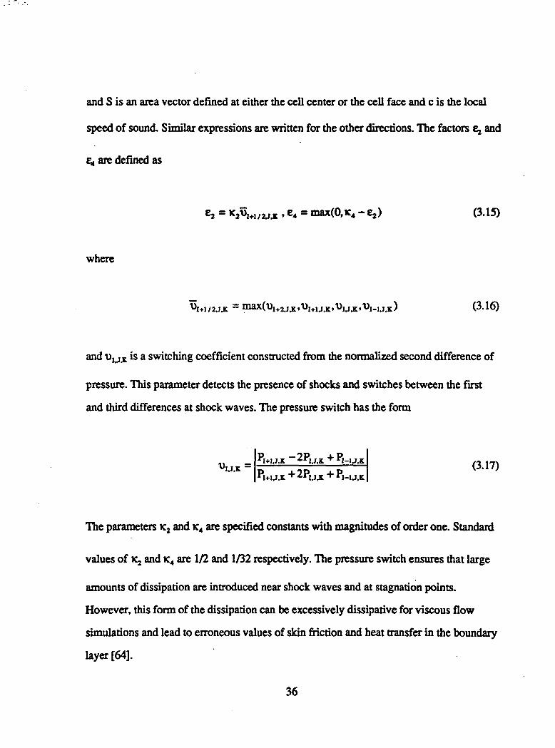
and S is an area vector defined at either the cell center or the cell face and c is the local

speed of sound. Similar expressions are written for the other directions. The factors Cj and

£4 are defined as

£a = K2^i+i/w.r • e4 = max(0,K4 - ej) (3.15)

where

,'Uw>K,'UI_u>K) (3.16)

and UU£ is a switching coefficient constructed from the normalized second difference of

pressure. This parameter detects the presence of shocks and switches between the first

and third differences at shock waves. The pressure switch has the form

M+J.JJC 2P, j K 4- PI-I J,K

M+U.K + "I.J.K + M-1J.(3.17)

The parameters K2 and K4 are specified constants with magnitudes of order one. Standard

values of iq and K4 are 1/2 and 1/32 respectively. The pressure switch ensures that large

amounts of dissipation are introduced near shock waves and at stagnation points.

However, this form of the dissipation can be excessively dissipative for viscous flow

simulations and lead to erroneous values of skin friction and heat transfer in the boundary

layer [64].

36

3.2.2 Modified Adaptive Dissipation

The Standard Adaptive Dissipation model can be modified to reduce the excessive

levels of dissipation introduced in viscous simulations by redefining the parameters

scaling the first differences in Equation (3.13b). For example, the scaling in the I

direction becomes

This leads to different scalings of the dissipation along each of the coordinate directions.

However, a directional dependency is introduced that can degrade the convergence rate

of the solution on highly stretched computational meshes. Swanson and Turkel [65] have

demonstrated that this problem can be alleviated by redefining the spectral radii used in

Equation (3.18) to produce an anisotropic scaling. The modified spectral radii have the

form

1 + (3.19)

where the exponent m has values of order one. In the baseline code, m is set to 1/2. The

parameter e, is also modified by restricting its maximum value to 1/2.

3.2.3 Flux-Limited Adaptive Dissipation

Both the SAD and MAD formulations exhibit pre- and post-shock oscillations

without careful tuning of the K2 parameter. Jameson [62] has introduced an alternative

formulation of the adaptive dissipation by redefining the coefficients scaling the first and

37

third differences in terms of flux limiters similar to those employed in MUSCL difference

schemes. The flux limiters act to locally switch the central differencing scheme to a first-

order upwind scheme at shock waves allowing shocks to be captured without oscillations.

In the flux-limited scheme, the dissipative flux at a cell face is defined as

(3.20)

where L is the limiter function and e is the first difference of the solution defined by

Equation (3.13b) but scaled by the factor

and X is again the spectral radii The parameter, f), is defined as

P = min^ , K2^l/UiK + K4 J (3.22)

The limiter function , L, is defined for two arguments, a and b, as

L(a,b) = [s(a)+s(b)] min(lal.lbl) (3.23)

where s(a) equals 1/2 when a is greater than or equal to zero and assumes a value of -1/2

when a is less than zero.

38

3.2.4 Matrix Based Dissipation

The dissipation given by Equation (3.12) applies the same scaling to all the

components of the flux. This scale factor is approximately the largest eigenvalue of the

Jacobian matrix, A. This can lead to excessive smearing in viscous regions because all

the characteristic waves that form the flux are scaled by the same coefficient which is

proportional to the fastest wave speed. Swanson and Turkel [63] have proposed an

alternate formulation similar to Roe's scheme where the scalar coefficient in Equation

(3.12) is replaced by a matrix defined by

|A| = TjAjT1 (3.24)

where A is a diagonal matrix given the similarity transformation

A = T'AT (3.25)

The transformation matrices, T and T4, are constructed from the eigenvectors of the flux

Jacobians [66]. For the Euler and Navier-Stokes equations, the diagonal elements of A

are given by the five eigenvalues of the flux Jacobian matrix, A, which can be written for

each coordinate direction as

39

where U is the contravariant velocity given by Equation (3.14b) and S is the area vector

along any coordinate direction. When the matrix, A, can be diagonalized, IAI can be

replaced by a matrix function of the form [67]

IAI =

(y-l)E4]

where I is the identity matrix. The matrices E,, Ej, E,, and E4 are written as

E,=

oUw

vO

W<J)

-u-u2

-uv— UW

-uH

-v-vu-v2

— vw-vH

-w— wu— wv-w2

-wH

1"uV

wH

(3.28a)

E2 =

0-SEU S2

-s,u s,s,-s.u s.s.

0 0 0

s2

-U2 US. US, US, 0

40

-u s,-uU uS,

-vU vS.

-wU wS,

-HU HS,

'0 0

S,4> -uS,S£ -uS,

S^ -uS,

_U<|> -uU

s,uS,

vS,wS,HS,

0-vS,-vS,-vS,

-vU

s.uS.vS,wS.HS,

0-wS,-wS,

-wS,

-wU

o"0000

»

0"s,s,s.u_

(3.28d)

where H is the total enthalpy and <}> = (u2 + v2 + w2)^. The special form of IAI given by

Equation (3.27) allows an arbitrary vector of to be multiplied by IAI without computing

the full matrix. Therefore, terms such as lAle^Q^ can be computed efficiently. The

flow variables used in the matrix equation are computed at each cell face by simple

arithmetic averages of the variables on either side of the face. Roe's scheme can be

recovered by replacing the arithmetic averaged variables with Roe's averaged variables.

As in Roe's scheme, the eigenvalues defined by Equation (3.26) must be modified to

maintain sufficient levels of dissipation at stagnation points and sonic lines because Xt is

zero at stagnation points while X4 and Xs vanish at sonic lines. Therefore, the values of the

eigenvalues are limited as

= max(|X1|,V1p(A)) (3.29a)

41

|X4| = max(|X4|,Vnp(A)) (3.29b)

|X5| = max(|X5|, VBp(A)) (3.29c)

where V, and Vn are constants and p(A) is the spectral radius of A defined by Equation

(3.14a). The constants, V, and Vn, are determined from numerical experimentation and

have typical values of 0.3 and 0.2, respectively. Further details of the formulation and

application of the matrix based dissipation are given in References [68] and [69].

3.3 Boundary Conditions

The TEAM code has options for a wide variety of boundary conditions for both

external flows such as wings and fuselages and internal flows such as engine inlets and

exhaust nozzles. The multi-zone formulation of the baseline code enables the simulation

of the flow about complex geometries such as a complete airplane. A patched or

composite grid system can be generated in which the computational domain is broken

into several grid zones that abut at defined zonal boundaries. In the baseline code,

boundary values are defined at the centers of a layer of "ghost" or image cells that

surround the boundary surfaces of each zone. The first layer of cells inside the boundary

are designated as boundary cells. For external flow simulations, the boundary conditions

must be defined at the far-field, body surfaces, and fluid boundaries such as wakes,

symmetry planes and zonal interfaces. Each type of boundary condition will be discussed

separately.

42

3J.I Far-Field Boundary Conditions

The far-field boundary conditions in the baseline code are obtained using the non-

reflecting characteristic boundary conditions introduced in Reference [44]. These

boundary conditions define the flow quantities in the boundary cells using the appropriate

number of characteristics entering and leaving the boundary. This procedure allows the

flow to enter and leave the finite computational domain without generating reflected

waves that can destabilize or retard the solution.

For subsonic flows, the boundary conditions are obtained from the local Riemann

invariants for a one-dimensional flow normal to the cell faces that make up the boundary

surface. The subsonic inflow boundary conditions are obtained from two incoming

characteristics and one outgoing characteristic. At the boundary, the Riemann invariants

can be defined in terms of the free-stream values at infinity and values extrapolated along

the characteristic line from the interior domain as

TIC" (330a)

(330b)

where q,.. and q^ are magnitudes of normal velocities of the flow variables at the cell

face defined using either the free-stream values of the flow variables or the values

defined in the boundary cells and the normal vector at the cell face. The variable c is the

speed of sound. The Riemann invariants are used to define the magnitude of the normal

component of velocity and the speed of sound on the boundary as

43

= - (R . + RJ, cb = (R. - R J (3.31)2 4

The values for density, pressure and velocity in the ghost cells can now be defined

using the values of q, and c on the boundary and values of entropy and tangential velocity

obtained from either the free-stream or extrapolated flow variables. The sign of die

contravariant velocity defined by Equation (3.14b) and obtained from the extrapolated

flow variables and the metrics at the cell face is used to distinguish between inflow and

outflow boundaries. For inflow boundaries, the flow variables are defined using the

following relations

s = pl/p. , P = (•cJ/Y)l*M) . P = pc2b/Y (3.32a)

(3.32b)

where s in the entropy and n is the normal vector at the cell face. For outflow boundaries,

the flow variables are obtained using Equations (3.32a) and (3.32b) with the values at

infinity replaced by the values extrapolated from the interior.

For supersonic flow, all characteristics directions either enter or leave the

computational domain. At supersonic inflow boundaries, the flow variables are fixed to

their free-stream values. For supersonic outflow boundaries, die flow variables are set to

the values in the boundary cells of the outflow boundary. This is equivalent to a zero

order extrapolation of the flow variables.

33.2 Solid Surface Boundary Conditions

For both the Euler and Navier-Stokes Equations, the solid surface boundary

conditions are imposed by setting the mass flux normal to the boundary to zero. In the

44

inviscid flux, the zero mass flux condition is implemented by setting the contravariant

component of velocity normal to the boundary face to zero. This is accomplished

automatically for the Navier-Stokes equations by imposing the no-slip condition obtained

by setting the velocities u, v, and w to zero for steady flows and equal to the surface

velocities, x, , yt and zt , for unsteady flows. For Euler simulations, the surface velocities

can be obtained from extrapolated values of the contravariant velocities tangent to the

cell face. In Navier-Stokes simulations, the no-slip conditions is imposed by setting the

values in the ghost cells such that a simple average of the ghost cell values with the

boundary cell values gives the appropriate surface velocity. For steady simulations, this

implies that the ghost cell values are obtained by reflection of the three components of

velocity in the adjacent boundary cells. For the cell centered finite volume scheme,

velocities are not required on the surface to form the inviscid flux. Only the pressure at

the cell face is required.

The baseline code has several different procedures of varying degree of accuracy for

defining the surface pressure. For steady flow simulations, the simplest and most stable

approximation is a zero order extrapolation of the pressure from the boundary cells. This

is consistent with the assumption of a zero normal pressure gradient A more accurate but

less stable procedure is to compute the pressure from the normal momentum equation.

For unsteady inviscid flows, the pressure gradient at the surface can obtained from the

solution of a normal momentum equation of the form [70]

(3.33)

45

where Ub and vb are the flow and surface velocity vectors at the surface cell face, n is the

normal vector at the cell face, and Vp is the gradient of pressure. The operator D /Dt is

the material derivative, 9 /9t + (v» V). For viscous flows, Equation (3.33) reduces to

(3.34)Dt

For inviscid steady flows, Equation (3.33) becomes

(3.35)

Equation (3.35) reduces to the zero normal pressure gradient assumption for steady

viscous simulations. Solution of the preceding equations requires values of velocity,

density, and pressure extrapolated from the interior. Several different approaches for

defining the extrapolated variables used in the solution of the normal momentum

equation were evaluated in the development of the baseline code. A complete description

of the various methods used in the TEAM code is given in Reference [40].

333 Fluid and Symmetry Plane Boundary Conditions

Fluid boundaries occur when two grid zones abut at a common interface or at branch

cut where two boundaries or surfaces of the same grid zone coincide. Both types of fluid

boundaries are characterized by an interface surface that connects the two zones or grid

segments. The baseline code supports three distinct classes of interfaces. The first type of

interface is referred to in the TEAM code as a Class 1 interface. For Class 1 interfaces,

the grid points on the interface are the same for both zones or grid segments. A Class 2

interface is formed when the interface is composed of a dense grid from one zone and a

46

coarse grid from the abutting zone that shares common points with the dense grid at some

regular mesh spacing on the dense grid. For instance, the coarse grid might consist of

every second or third point in the dense grid. In both the Class 1 and Class 2 interfaces,

the zones are connected at common grid points. The baseline code allows a third class of

interface, Class 3, in which none of the grid points in the two zones are required to

coincide. The only restriction on the Class 3 interface is that the interface points must lie

on the same level surface.

The accuracy and efficiency of multi-zone discretization procedures depends on the

level of global conservation maintained during the solution. It is important that ghost cell

values at zonal interfaces are specified in a manner that assures global conservation. For

Class 1 boundaries, conservation is maintained by injecting the boundary cell values from

the abutting zones into the ghost cells of the adjoining zone. Therefore, the spatial order

of accuracy of the flux conservation at the interface is the same as for the interior cells.

However, Allmaras [71] has shown that second order accuracy is not possible for Class 2

and Class 3 boundaries if strict conservation is enforced. In addition, first order accuracy

can only be obtained using appropriate characteristic extrapolation procedures that are

computationally expensive. In the baseline code, a zeroth-order extrapolation procedure

proposed by Allmaras is used that maintains conservation across the fluid boundaries at

Class 2 and Class 3 interfaces.

As shown in Figure 3.3, the definition of the ghost cells for the coarser of the two

grids at a Class 2 or Class 3 interface is defined by an area weighted average of boundary

cell data from both the coarse and fine grids. In Figure 3.3, the boundary cells in each

zone are designated by B, the ghost cells by the letter G, and S is the corresponding cell

face area. The ghost cell values for the dense grid is defined using the values in the

boundary cell whose interface surface the corresponding surfaces in the dense grid. For

Class 3 interfaces, the number of grid cells and areas used in the extrapolation is set to a

47

maximum value, usually four, to reduce storage requirements. In addition, each grid

surface must be searched to define the appropriate cells and areas to be used in the

extrapolation.

Zone 1 Zone 2

B,,

B12

B»

B14

Gn

G12

G,,

G14

GU=B21

G12=B21

0.3=8,2

0,4=6,2

Ga=C 1BU4C2B,24C j

Figure 3.3 Class 2 and Class 3 Fluid Boundary Conditions

The ghost cell values at planes of symmetry are obtained by reflecting the appropriate

boundary cell velocity component across the plane and injecting the remaining flow

variables from the boundary cells.

48

3.4 Explicit Solution Procedure

The explicit solution procedure in the baseline code is the multi-stage Runge-Kutta

time stepping scheme introduced by Jameson et al. [44] in the FLO57 code. Because of

the restrictions on solution time step inherent in all explicit formulations, three different

types of acceleration techniques are employed in the TEAM code for steady flow

simulations. For steady Euler simulations, enthalpy damping can be employed to force

the solution to the steady state condition of constant total enthalpy. In addition to

enthalpy damping, the implicit residual smoothing procedure introduced by Jameson [72]

can be used to increase the maximum time step of the multi-stage scheme. Finally,

spatially varying time steps can be used for steady flow simulations to reduce the time

required to reach a steady state solution. Spatially varying time steps act as a

preconditioner on the discretized equations that relaxes stiffness in the solution due to

local variations in the flow variables. The accelerated form of the multi-stage time

stepping scheme provides a cost effective solution procedure for the steady Euler

equations. However, the severe time step restrictions imposed by the explicit formulation

make the scheme ill-suited for Navier-Stokes and unsteady flow simulations.

3.4.1 Multi-stage Time Stepping

The discretized form of Equation (2.3) for stationary grids can be written for each

cell volume as

Fv-D = 0 (3.36)dt

49

where F, is the net inviscid flux, Fv is the net viscous flux, and D is the net dissipative

flux through the cell volume. For stationary grids, the volume ,V, is constant Therefore,

Equation (3.36) can be written as an ordinary differential equation of the form

—+R(Q) = 0 (3.37)dt

where R(Q) is the residual defined by

(3.38)

A multi-stage explicit time stepping scheme based on the Runge-Kutta method is used in

the baseline code to integrate Equation (3.37) in time. The m-stage procedure for

advancing the solution from a time level n to n+1 can be written as

Q(0)_Q«

(3.39)

QW _ QfrB-l) .

50

where At is the time step and the parameters, otm, are constants that vary with the number

of stages and residual smoothing. For most simulations, the viscous and dissipative

components of the residual are computed only once and held constant for all stages. For

the four stage scheme used in this research, the a coefficients have values in ascending

order of 1/4,1/3,1/2, and 1. In the absence of residual smoothing, die four stage scheme

is stable for Courant (CFL) numbers up to 2 ->/2 for 1-D model problems. Residual

smoothing and enthalpy damping can extend the CFL limit of the four stage scheme to a

value of 6.

3.4.2 Enthalpy Damping

Enthalpy damping is implemented for steady Euler simulations by adding a forcing

term of the form

opH

ctpuH

apvH

apwH

apH

(3.40)

to the residual, R. The parameter ,a, is a user specified constant In addition, the non-

dimensional total energy, total enthalpy and pressure are redefined as

(3.41)

51

Therefore, the forcing function acts to drive the value of total enthalpy in each cell to the

free-stream value as the solution converges.

3.43 Residual Smoothing

The concept of residual smoothing was first introduced by Lerat as part of a family of

implicit schemes based on Lax-Wendroff type differencing [73]. Jameson applied the

procedure to the Runge-Kutta multi-stage scheme [72]. The basis of residual smoothing

is to replace the residual defined by Equation (3.38) with an effective value defined by an

implicit smoothing or averaging operator. The implicit smoothing acts as a preconditioner

by damping out local high- frequency variations in die residual. The smoothing operation

can be written in three dimensions as

-e(82 + 62+62))Rs=R (3.42)

where 82 is the central difference operator for second derivatives, Rs is the smoothed

value of the residual and e is smoothing parameter that can be either constant or vary in

space. In practice, Equation (3.42) is solved by approximately factoring it into a sequence

of three scalar tridiagonal operators of the form

(3.43)

For constant values of e, a one dimensional stability analysis shows that the stability of

the central difference scheme can be maintained for a given CFL number when the

smoothing coefficients satisfies the following condition

52

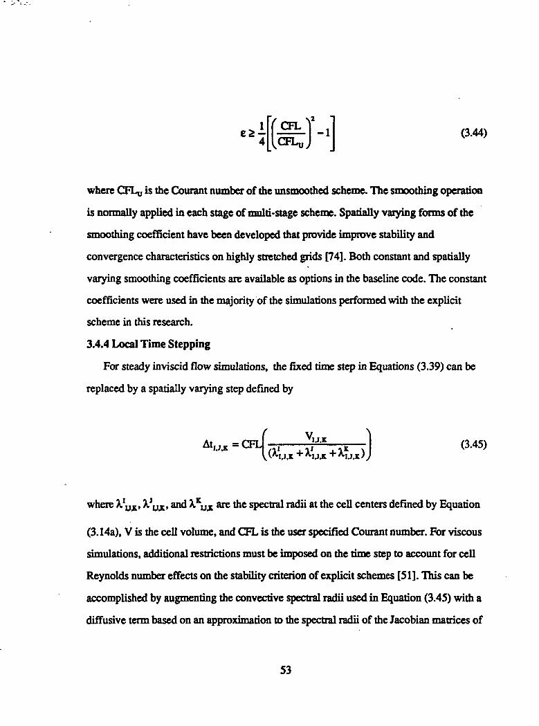
fel- (3.44)

where CFLu is the Courant number of the unsmoothed scheme. The smoothing operation

is normally applied in each stage of multi-stage scheme. Spatially varying forms of the

smoothing coefficient have been developed that provide improve stability and

convergence characteristics on highly stretched grids [74]. Both constant and spatially

varying smoothing coefficients are available as options in the baseline code. The constant

coefficients were used in the majority of the simulations performed with the explicit

scheme in this research.

3.4.4 Local Time Stepping

For steady inviscid flow simulations, the fixed time step in Equations (3.39) can be

replaced by a spatially varying step defined by

= CFL . K . I (3-45)•*" A'U.K"

where X!u^, XJ

UJC, and XKUZ are the spectral radii at the cell centers defined by Equation

(3.14a), V is the cell volume, and CFL is the user specified Courant number. For viscous

simulations, additional restrictions must be imposed on the time step to account for cell

Reynolds number effects on the stability criterion of explicit schemes [51]. This can be

accomplished by augmenting the convective spectral radii used in Equation (3.45) with a

diffusive term based on an approximation to the spectral radii of the Jacobian matrices of

53

the viscous flux terms [75]. The general form of the diffusive term along each coordinate

direction at a cell center can be written as

i - Ji.*— 3p

s;+s;+sn py ,y(is,s,i+is,s.{ v J^lft' T v (3.46)

The time step can then be computed with the spectral radii terms used in Equation (3 AS)

replaced by the sum of the convective and viscous spectral radii. These values are also

used in the construction of the artificial dissipation. The use of local time steps for steady

flow simulations converts the time-accurate multi-stage time stepping scheme to a

"pseudo-time" stepping scheme. The magnitude of the step is computed to satisfy

stability criterion and is not set to resolve discrete time-varying phenomena. The

objective is to obtain a steady state in the smallest possible number of steps. The time

step is usually updated at the start of each step. For Euler simulations, the time step can

be updated at fixed intervals of up to twenty steps without seriously impacting the

convergence rate.

3.5 Implicit Integration Procedure

The severe time step restrictions of the explicit multi-stage scheme make them

unsuitable for large scale unsteady viscous simulations. Implicit solution schemes are

favored for unsteady flow simulations because they allow much larger time steps to be

taken without sacrificing the stability of the scheme. However, the computational effort

per step for most practical implicit schemes can be several time the effort for explicit

formulations. This is due to the fact that implicit formulations are based on a local

54

linearization of the flux vector at time level n+1 about the previous time level that

produces large banded matrix systems of equations. This linearization is obtained from a

local Taylor's expansion of the form

= F° + ?L^1 At + 0(At2) (3.47)oQ dt

where 3P /3Q is the flux Jacobian. Replacing dQ1*1 /dt with

dt At(3.48)

yields the common form of the linearized flux. For AQ""1 = Q^1 - Q", Equation (3.47) is

approximated by

AQ"41 (3.49)dQ

Substitution of Equations (3.48) and Equations (3.49) into the discretized forms of

Equations (2.1) and (2.3) yields a general implicit scheme which has the following

differential form in the general curvilinear coordinates £, T\, and £:

~R(Q") (3.50)

55

where Dt , Dn, and D^ are difference operators, A°, B°, and C1 are the flux Jacobian

matrices along each coordinate direction, and I is the identity matrix. The scheme is

second-order accurate in time when the parameter, a, equals 1/2. The scheme is first

order-accurate for all other values of a. R is the residual defined by

(3.51)

where F, G, H, Fv, Gv, Hv are the inviscid and viscous flux's along the three coordinate

directions. For a true time-accurate linearization of the complete flux, the flux Jacobian

matrices contains contributions from both the inviscid and viscous fluxes. Formation of

the inviscid and viscous Jacobians is computationally expensive. Therefore, a common

approximation for Navier-Stokes simulations is to neglect the viscous contributions and

form the Jacobian matrices from the inviscid flux components. For appropriate levels of

dissipation and time steps, this approximation has a minimal impact on solution accuracy

and convergence.

3.5.1 Commonly Used Implicit Schemes

Expansion of the left hand side of Equation (3.50) leads to a large banded block

matrix system of equations. Solution of this system by direct inversion in three

dimensions is impractical for real-world problems. Therefore, considerable research has

been devoted to developing computationally efficient indirect solution procedures. These

indirect methods fall into two classes: approximate factorization schemes based on the

Douglas-Gunn ADI method [76] or the more recently developed relaxation schemes

[77,78].

56

The most widely used ADI schemes were introduced by Briley and McDonald [79]

and Beam and Wanning [80] in the mid 1970's. Both schemes replace the unfactorcd

implicit operator in Equation (3.50) with a product of three one dimensional operators

defined along each coordinate direction. In die three-dimensional Beam-Warming

scheme [81], Equation (3.50) is approximated by

(3.52)

For central differencing, each operator in Equation (3.52) is a block tridiagonal matrix

which can be solved by variants of the Thomas algorithm for tridiagonal systems [51].

Although unconditionally stable in two-dimensions, the factorization given by Equation

(3.52) can be shown to be unstable in three-dimensions without the inclusion of large

amounts of implicit and explicit artificial dissipation. Implicit dissipation is added by

including terms similar to Equation (3.12) in the implicit factors. The inclusion of fourth-

order dissipation leads to block pentadiagonal factors. Although more efficient than direct

simulation, the solution of the block matrix systems is still computationally expensive for

three dimensional problems. Another problem with the three factor scheme is that an

error term of order (At)3 is generated by the factorization that can severely impact the

convergence rate. Pulliam and Chaussee [66] have introduced a variation of the Beam-

Warming algorithm that uses symmetric diagonalization of the Jacobian matrices to

produce a stable scheme with scalar tridiagonal or pentadiagonal factors. This biggest

drawback of this scheme is that it is at most first order accurate in time.

The large factorization error of the three-factor ADI scheme has lead to the

development of two factor schemes which are of order (At)2 and stable in three

57

dimensions. Two factor schemes in common use are the partially flux-split scheme of

Steger et al. [82], the hybrid scheme of Sankar [83,84,85], the Lower-Upper (LU)

factorization scheme proposed by Jameson and Turkel [861 and Buning and Steger [87]

and the Symmetric-Gauss-Seidel variant of the LU scheme (LU-SGS) introduced by

Yoon and Jameson [88]. The flux-split scheme was applied by NASA researchers to a

wide range of problems [89,90]. The hybrid scheme is effective for solving flows about

wings and rotors [84]. The LU was not used extensively until the mid 1980's when

Jameson and Yoon [91] applied the scheme to the solution of the Euler equations. Other

researchers such as Whitfield [92], Buratynski and Caughey [93] and Yokota and

Caughey [94] successfully extended the scheme to solve both the Euler and Navier-

Stokes equations. Both the partially flux-split scheme and the hybrid scheme require

block tridiagonal inversions in two coordinate directions. The LU scheme requires block

diagonal inversions for each factor. The LU-SGS scheme can be constructed in forms that

require either block or scalar diagonal inversions.

The scalar diagonal form of the LU-SGS scheme has become the most popular of the

two factor schemes because of its low operation count and generally good convergence

characteristics. The scheme is especially suited chemically reacting flows because it

requires at most a block diagonal inversion of the Jacobian matrices. Therefore, its

greatest use has been in the area of chemically reacting and hypersonic flows [95,96,97].

Yoon and Kwack [98] implemented a three-dimensional version of the scheme for

solving the compressible Navier-Stokes equations and applied it to standard steady

transonic wing cases. This code has been extended using multi-grid to accelerate the

convergence to a steady state [99,100]. The scheme has been used successfully by Chen

and McCroskey [70,101] and Srinivasan et aL[102] for unsteady rotor analyses in both

hovering and forward flight Obayashi and Guraswamy [103] implemented a version of

the scheme in the ENS AERO code for the solution of coupled aeroelastic problems. An

58

attractive feature of die scalar form of the LU-SGS scheme is that with careful coding it

can achieve computational speeds that are competitive with explicit schemes. In addition,

it is a simple algorithm to implement because it requires no special matrix solvers. These

factors led to the selection of the scheme for this research.

3.5.2 The LU-SGS Scheme

The LU-SGS scheme has its roots in the LU scheme of Jameson and TurkeL This

scheme can be written as

LUAQ = -—R (3.53a)

where the factors L and U are

L = I + ̂ ( V* + V^B* + V;C*) (3.53b)

U = I +—(A. A' + A-B- + ACC") (3.53b)^^ \ * • /

and the operators, V?, V,,, V;, A^, A,,, and A^ are standard backward and forward

differences. The stability of the LU scheme is dependent on each factor being diagonally

dominant This is achieved by replacing the standard flux Jacobians with diagonally

dominant forms whose eigenvalues are either all positive (A*, B+, and C*) or all negative

(A", B", and C). The LU-SGS scheme is obtained by recasting the factors as Symmetric

Gauss Seidel relaxation sweeps [104]. After some algebra, Equations (3.53) become

59

(3.54a)

where

— I + -— ^ A —A + B —B + C Cj (3.54c)

CtAtu = i+—(A%A~+AnB-+\cr+A-+B*+cr) (3.54d)

Like the LU scheme, the Jacobian matrices must be diagonally dominant Yoon and

Jameson proposed approximate Jacobians that satisfy this condition. These Jacobians are

constructed from the standard Jacobians of the inviscid flux vectors augmented by then-

corresponding spectral radii. The approximate Jacobians have the forms

(3.55a)L

B*=i(B±p(B)I) (3.55b)

fi*-j(C±p(QI) (3.55c)

A general form of the matrices, A, B, and C is given in Appendix B. The spectral radii

such as p (A) are defined by

60

p(A) = Kmax[l X(A) l] (3.56)

where X(A) represent the eigenvalues of A and K is a constant £ 1 that is used to control

stability and convergence. With these definitions of the diagonally dominant Jacobians,

the operator, D, in Equations (3.54) can be written for a =1 as

D = l + (p( A) + p(B) + p(Q) I (3.57)

The L and U operators can then be written after expansion of the differences at a cell

center defined by the indices I, J, and K as

(3.58a)

q«+I) (3.58b)

With these operators, the solution of Equation (3.54a) can be obtained by forward and

backward relaxation sweeps that proceed from the lower left corner of a zone to the upper

right corner and then back. The sweeps are performed in the following order

Forward sweep:

-i AQ," K.,) (3.59a)

61

Backward sweep:

= DAQ," , - A.WACC, + B^ACC, + CT^AQ^ (3.59b)

Update Q:

It is important to note that the operator, D, is a scalar diagonal matrix. Therefore, the

intermediate and final corrections, AQ** and AQ0*1, are obtained by simple division. At

the boundaries, all off-diagonal values of the intermediate and final corrections are set to

zero.

For At=«>, the LU-SGS scheme can be recast to resemble a quasi-Newton or Newton-

like iteration scheme that does not require specification of an optimum CFL number or

time step. After multiplying through by V/At and setting At=«>, the diagonal operator, D,

becomes

D = [p(A) + p(B) + p(C)]I (3.60)

and the factor At/V disappears from the off-diagonal terms in the L and U operators. This

scheme cannot achieve the quadratic convergence of a true Newton method due to the

approximate Jacobians and Ac factorization error. However, linear convergence can be

demonstrated.

Another advantage of the LU-SGS algorithm is that it is completely vectorizable

when the forward and backward sweeps are performed in oblique planes defined by

62

I+J+K=constant such as the one shown in Figure 3.4. This can be achieved by either

reordering the three-dimensional arrays into two dimensions defined by the serial number

of the oblique plane and the addresses of the points on the plane or creating mapping

arrays that allow the existing three-dimensional array locations to be indexed indirectly.

The second approach was used in this research to avoid having to rewrite large sections

of the baseline code. The three-dimensional arrays containing the solution, etc. can be

taken into the solver routine as dummy arrays and redimensioned as a large one

dimensional vector. The location of any point in this vector can be defined by L = I + (J-

1)*MI + (K-1)*MI*MJ where MI, MJ, and MK are the maximum dimensions of the

corresponding three-dimensional array. The value of L at each point in the plane defined

by I+J+K=constant is stored in an integer array along with the number of points in each

plane, NP. These arrays provides the correct address for the required values on each

oblique plane.

K

Figure 3.4 Oblique Sweep Planes For LU-SGS Scheme

63

The solution scheme defined by Equations (3.59) is first order-accurate in time.

Higher order accuracy can be obtained by using Newton inner iterations [101,105] at

each time step. This procedure also helps minimize the factorization error. Matsuno [1061

has introduced the 6K scheme which is a variant of the inner iteration scheme that can

obtain k-th order accuracy in k sub-iterations. Lee and Kim [107] have used the 5K

approach with the LU-SGS scheme to calculate rotor flows in hover and forward flight

3.6 Moving Grid Procedures

The application of the discretized forms of the governing equations to moving grid

systems requires special treatments for calculating the flux, cell volume, and grid speeds.

In particular, Thomas and Lombard [108] have demonstrated that an additional geometric

constraint called the Geometric Conservation Law must be imposed for moving grid

systems to ensure that conservation is maintained for uniform flows. For non-uniform

flows, the cell volumes and grid speeds need to be computed in a consistent manner to

prevent grid induced errors. The geometric constraint can be expressed for discretizations

based on Equation (2.1) as

(3.61)ti 8(0

Equation (3.61) represents the conservation of volume for a moving cell. Similarly, the

integro-differential form of the law can be written as

64

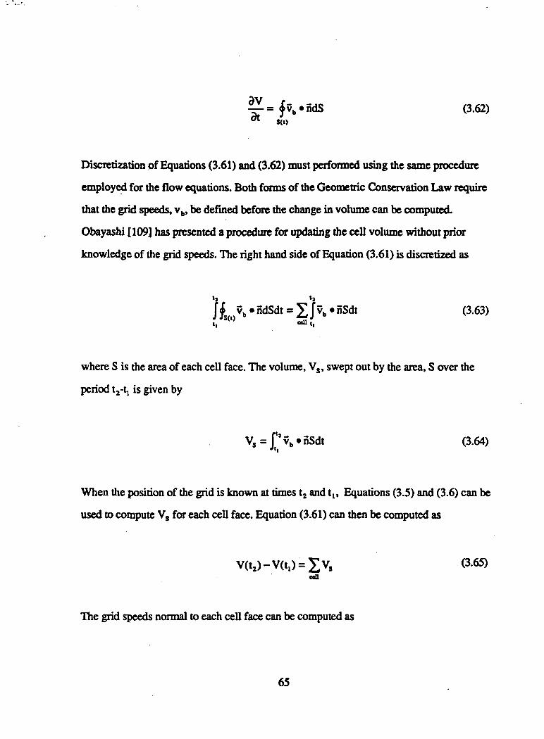
- ,-. — (3.62)31 m

Discretization of Equations (3.61) and (3.62) must performed using the same procedure

employed for the flow equations. Both forms of the Geometric Conservation Law require

that die grid speeds, vb, be defined before the change in volume can be computed.

Obayashi [109] has presented a procedure for updating the cell volume without prior

knowledge of the grid speeds. The right hand side of Equation (3.61) is discretized as

J J vb • ndSdt = £ Jvb • nSdt (3.63)"<0 «u

where S is the area of each cell face. The volume, Vs, swept out by the area, S over the

period t2-t, is given by

Vs= f t avb»nSdt (3.64)"i

When the position of the grid is known at times t2 and t,, Equations (3.5) and (3.6) can be

used to compute Vs for each cell face. Equation (3.61) can then be computed as

Vs (3.65)od

The grid speeds normal to each cell face can be computed as

65

(3.66)

For moving grids, both the implicit and explicit formulations contain an extra term

that is added to the residual For an implicit discretizations with Qn+I=Q1+AQ, (QV)0*1 is

replaced with (QVAQJV*1 and

(QV)B+l - (QV)n = AQV"*1 + Q"(V"*1 - Vn) (3.67)

The term, (y (V^-V11), is added to the residual This term vanishes for stationary grids

since the volume does not change. The change in volume is computed using the

Geometric Conservation Law. For many aeroelastic applications, the rate that the volume

changes with time is small and the Geometric Conservation Law can be neglected

without a severe impact on solution accuracy. Rapidly moving grid systems require the

Geometric Conservation Law for accurate solutions.

66

CHAPTER IV

DISTRIBUTED COMPUTING PROCEDURES AND

IMPLEMENTATION

This chapter describes die procedures used to convert the baseline Lockheed/AFOSR

multi-zone flow solver into a parallel flow solver for distributed computing systems. The

basic approach taken in developing the distributed flow solver was outlined in Chapter 1.

The following sections describe the Parallel Virtual Machine (PVM) software interface used

for interprocessor communications, the factors that effect communication performance on

distributed systems, the communication strategies employed in the solver, load balancing

procedures and details of the modifications made to the baseline TEAM code,

4.1 The PVM Message Passing Interface

The Parallel Virtual Machine (PVM) system was developed jointly by the Oak Ridge

National Laboratory, the University of Tennessee, and Emory University to provide a

standard message passing system for connecting homogenous and heterogeneous systems

of UNIX workstations into a large distributed parallel computing system termed a "virtualt

machine". The virtual machine allows a network of individual workstations to emulate a

large dedicated distributed parallel system such as the Intel Paragon. Unlike the Paragon

which has specialized internal high speed communications subsystems for interprocessor

67

communications, PVM communications are usually performed using slower external

network hardware systems such as Ethernet

Since it's inception in 1989, PVM has become the "de-facto" standard for distributed

computing on workstations. Recent versions of PVM were extended to support large

multiprocessor systems such as the Intel Paragon and the Cray T3D systems. The

popularity of PVM can be attributed to its simple but versatile software interface that

supports both FORTRAN and C and its ability to run on a wide variety of hardware

platforms. The major drawback of the system is relatively poor communications

performance [110]. This has led to the development of an alternate interface, die Message

Passing Interface (MPI), that is being adopted as an ANSI standard system [111].

However, MPI had not reached the same level of maturity as PVM when this research was

initiated. Therefore, PVM was selected for this research.

The PVM system is composed of two components. The first component is a UNIX

program called a daemon that runs on each processor in the virtual machine. The daemon

functions as a server that handles process control, synchronization, fault detection and

message routing between processors. On message passing systems, messages are sent as

packets over interprocessor communication channels. The standard PVM system uses both

the UDP and TCP/DP UNIX communications protocols [112] to route messages between

tasks. The UDP protocol is used for communication between daemons on different

machines. The TCP protocol is used for local communication between daemons and tasks

on the same machine. Current versions of PVM also allow tasks to bypass the daemon and

communicate directly with each other using the TCP protocol. The daemons provide

buffers to hold incoming and outgoing messages and ensure that the messages are

processed in the correct order. The daemons must be started manually from a list of

available hosts supplied by the user. Individual tasks can spawn other tasks on processors

belonging to the virtual machine.

68

The second component of the PVM system is a library of user callable routines in

FORTRAN or C for message passing, spawning processes, sequencing tasks, and

dynamically reconfiguring the virtual machine. These routines must be linked to the users

application. The message passing routines form die core of die programming interface.

They allow users to open message buffers dial can be packed widt data of varying data type

and send the data to individual processors widi unique message tags. The PVM software

performs die data conversions required when binary data is passed between machines of

different architectures. This simple but complete library allows users to develop parallel

applications with minimal modifications to their existing code.

Three versions of die PVM system were used in tiiis research. The first two version of

PVM used were PVM 3.1.4 and 3.2.S that were released in die public domain by Oak

Ridge Laboratories. The final version of PVM used in this research was die IBM PVMe

system [113] developed by IBM for dieir SP1 and SP2 distributed parallel systems. PVMe

is based on version 3.2.6 of die public domain PVM. The major difference between die

public domain version of PVM and PVMe lies in die communication protocol used for

interprocessor communications. PVMe does not use TCP/IP for interprocessor

communications. Communication is performed directly between all tasks using die Allnode

or High Performance Switch (HPS) hardware subsystems on die SP1 and SP2 and die

Communication Subsystem (CSS) communication software interface [113,114].

4.2 Communication Strategics

The distributed flow solver is implemented by using die domain decomposition inherent

in die baseline multi-zone solver to map individual grids or sets of grids to separate

69

processors. The solution on each grid is performed concurrently. Therefore, the

performance of the distributed solver is dependent on the efficiency of task sequencing and

data communication procedures used in the solution process. The goal is to keep the ratio

of communications time to solution time as low as possible. The communications

performance is dependent on the speed of the communications channels connecting the

processors, the number of messages that must be passed between processors, and the type

of network topology used in the distributed system. Therefore, the types of

communications strategies adopted for die distributed solver must take into account the

network specific factors that effect communication performance.

4.2.1 Communications Performance Factors

The speed of the communications channels in a distributed system is driven by two

factors, latency and bandwidth [113]. Latency is defined as the time interval between the

instance at which the program institutes a call for a data transmission and the instance at

which the actual transfer occurs. This time interval can be thought of as the time required to

send a zero length message between nodes. Latency depends upon characteristics of the

communications hardware and the layers of software involved in packing and transmitting

data. Bandwidth is defined as the total available bit rate of a digital channel and represents

the maximum speed of information transfer between nodes. System bandwidth is

determined by the speed and type of the network or communications subsystem connecting

processors and the overhead incurred by die control data added by die communication

protocol during information transfer.

The type network connecting die nodes in a distributed system also plays a

significant role in die performance of a distributed flow solver. There are two basic types of

communications networks: circuit-switched and packet switched. Circuit switched

networks create dedicated paths between nodes and prevent simultaneous traffic over die

70

I paths at communication time. Packet-switching networks segments each message into

packets with unique destination tags that are sent over the network. Ethernet is the most

widely used example of a packet-switching system.

| Networks are also characterized by their physical and electrical topologies [1 15]. These

I topologies define whether die network is a shared medium where only a single processor

I can send messages over die network at a time or a switched network where two or moreI! nodes can communicate with each other simultaneously through a switched circuit

I Networks such as Ethernet and FDDI are examples of shared medium networks. Dedicatedi

communications subsystems such as die High Performance Switch on die IBM SP2 are

usually switched networks.i

The performance of shared medium networks such as Ethernet deteriorates quickly with

increasing numbers of nodes and users. This is because Ethernet is a broadcast busI1 technology that communicates in half-duplex. This means diat the end nodes on an Ethernet

I system cannot simultaneously send and receive messages. All nodes on die network share a

single communications channel or bus. Messages are broadcast to each node which is

responsible for determining which messages it should receive and which messages toI

ignore. A message collision can occur when two nodes try to transmit data simultaneously.

When a collision occurs die nodes must wait a random amount of time before retransmitting

the messages. Therefore, placing several messages on die bus at one time increases die

chances of message collision and reduces die system throughput. These factors limit die

standard Ethernet to a diroughput of 10 megabits per second Recently, switching

technology has been introduced that can raise die performance of Ethernet Switched

systems offer a much higher transfer rate tiian standard Ethernet For example, die High

Performance Switch system on die IBM SP2 is a bi-directional system with a peak rate of

320 megabits per second in each direction [114].

71

MANAGER

V '

MANAGER SENDS INITIAL DATA,GRIDS, BOUNDARY UPDATES, ANDSYNCHRONIZES TASKS:

MANAGER RECEIVES BOUNDARYDATA, CONVERGENCE DATA, ANDFINAL SOLUTION:

WORKER RECEIVES INITIALDATA, COMPUTES TIME STEP,AND CALLS FLOW SOLVER

RETURNS BOUNDARY DATA,AERO DATA, AND FINALSOLUTION

Figure 4.1 The Manager-Worker Strategy

solution steps. The manager is responsible for reading in the solver initialization and

control parameters, the computational grids, and the solution arrays required to restart the

solution from a previous run. The workers contain the actual Euler and Navier-Stokes

solution routines. Prior to the initial solution step, the manager assigns grids to die

individual processors and sends the appropriate initialization data and grids to each

processor using the PVM interface. The workers compute the initial time steps and

initialize the ghost boundary arrays used in the baseline code. At the start of each step,

73

boundary array data for each processor is sent to the manager that stores the data in a global

buffer and then sends each processor the boundary data it requires from grids on other

processors. The workers wait until they receive the updated boundary data and then

perform a solution step and update their local boundary arrays. Each worker then returns

convergence information to the manager, updates the time step, sends die appropriate local

boundary arrays back to the manager, and waits to receive the updated boundary data from

the manager before continuing with the next solution step. This process is repeated until a

maximum number of steps are performed or a specified convergence criterion is reached

The biggest advantage of the Manager-Worker strategy is the reduced complexity of the

control logic required to synchronize the required data exchange between processors. By

routing the data exchange through the manager, die number of possible data paths is

reduced to die number of worker processes. If the workers are allowed to communicate

directly with each other, a maximum of N(N-l)/2 two way paths would be required for N

workers if each worker was required to communicate witii every other worker in the

system. A second advantage of die Manager-Worker approach is that the workers do not

have to be the same program as required by die Single Program Multiple Data (SPMD) [9]

programming model. This simplifies die addition of other types of modules such as

structural analysis routines or modules for design optimization into die solution process.

One disadvantage of die Manager-Worker strategy is tiiat a processor must be dedicated to

die manager which can be a problem in systems widi a small number of available

processors. The biggest disadvantage of die Manager-Worker strategy is that routing data

back and forth tiirough die manager creates a communications bottleneck widi increasing

numbers of processors. This bottleneck can lead to excessive amounts of worker idle time

as they are forced to wait while die manager accumulates boundary data and then sends it to

the appropriate processors. This problem can be acute on dedicated distributed systems

74

with large numbers of available nodes. Therefore, an optional strategy called Worker-

Worker that allows workers to communicate directly with each other was implemented.

4.2.3 The Worker-Worker Strategy

The Worker-Worker strategy was implemented as a modification to the Manager-

Worker approach. The manager was maintained to provide the same initialization, IAD, and

synchronization functions as the Manager-Worker code. However, the appropriate zonal

boundary data required by a worker at the start of each step is obtained directly from the

other workers. The manager signals the start of each new step and the workers first send

out their updated solution data to appropriate processors and then wait to receive the

boundary data they require from the other workers. The workers send convergence data

back to the manager at the end of each step. The connections between processors are

determined at the start of the solution in the manager from the baseline code's boundary

condition data set and predefined grid-to-processor maps.

4.3 Load Balancing

Load balancing is the process of dividing the computational work among individual

processors in manner that keeps all processors busy and reduces the idle time spent

waiting for data. This idle time is imposed on the processors with the lightest loads by the

synchronization required by the zonal boundary update process. The lightest loaded

processors might have to wait until the heaviest loaded processor finishes before it gets the

boundary data it needs to continue the solution. Therefore, proper load balancing is crucial

if the expected speedup of the distributed parallel version of the TEAM code over die serial

version is to be obtained. An efficient load balancing procedure must account for both the

75

C.-Z-

total number of grid points mapped to each processor and the computational speed of each

processor. These factors are known quantities that remain static during the course of a

solution. Additional factors such as system load and communications overhead can also

degrade performance and should be included in the load balancing process to obtain the

optimum performance. However, these factors cannot be fixed prior to the start of a

solution and must be accounted for dynamically. These factors lead to two general types of

load balancing: static and dynamic.

Static balancing procedures are effective on dedicated or lightly loaded distributed

systems and are the easiest to implement The load balance is computed at the start of the

solution and held fixed to its initial distribution. In dynamic load balancing, the

performance of the system is monitored during the course of the solution and the load on

each processor is modified at intervals to maintain the optimum performance. Dynamic

balancing can be effective on heavily loaded network based systems [37]. However, the

solution overhead required for dynamic balancing can be several time that of static

balancing. This is particularly true for a structured multi-zone flow solver such as the

baseline code which requires an exact definition of the zonal boundaries to form the buffer

arrays that hold the required ghost boundary data. In dynamic load balancing system, the

dimensions of the buffer arrays would have to be adjusted dynamically or fixed to an

inappropriately large number. In addition, the fixed nature of most structured multi-zone

grid systems make dynamic load balancing impractical for use with an existing flow solver.

The existing zonal interfaces have to be maintained in addition to any new interfaces

introduced by the balancing procedure. Unstructured grids are more amenable to dynamic

balancing because they treat the grid as a cloud of points surrounding the body surfaces

with no zonal boundaries. Therefore, clusters of points can be assigned to processors

without the need to maintain an existing zonal interface. An effective dynamic load

balancing procedure for unstructured grids has been given by Vidwans et al. [118]. A

76

run-time load balancing procedure for structured grids has been given by De Keyset et al.

[119]. This procedure uses a specialized communications and control software system to

perform the required load balancing.

The problems inherent in implementing a dynamic load balancing procedure in the

distributed flow solver led to the adoption of three different static procedures. The first

procedure used was a purely ad hoc approach in which grids were assigned to processors

manually. The approach taken was to assign the largest grids to the fastest processors with

the most memory. Multiple grids were allowed to reside on a single processor to

accommodate the situation where there are more grids than processors. Therefore, two

smaller grids could be assigned to a processor to give approximately the same load as a

single larger grid on a separate processor.

In addition to the ad hoc approach, two automated static balancing procedures were

implemented and evaluated. The first automated procedure used is a version of the Task

Queue approach introduced by Johnson [120]. The second automated procedure used in

this research is the modified form of the heuristic Crutchfield [121] algorithm introduced by

Smith and Palas [13]. The details of the two automated procedures are given in the

following sections.

4.3.1 Task Queue Load Balancing Procedure

The Task Queue load balancing scheme is a modified form of the dynamic Pool of Task

approach [9] in which a master program creates a pool of tasks that are sent to worker

programs as they fall idle. The Task Queue procedure starts by forming a queue of

available worker processors sorted with the fastest processors at the top of the queue. A

second queue is formed from the available grids with the largest grids assigned in

descending order to the fastest processors. When all the processors are assigned a grid, a

solution step is performed on each of the first N grids where N is the number of processors

77

and the order in which the processors finish the first set of grids is stored. The next set

grids in the grid queue are assigned to the processors in die order in which the first set of

grids finished and a solution step is taken. This procedure is repeated until all the grids in

the grid queue have been assigned to assigned processor. The final distribution of grids on

processors is held fixed for the remainder of the solution. With the Task Queue approach,

the processors that finish first for each set of grids will continue to receive more grids until

all the grids are assigned. The advantage of the Task Queue procedure is that the effect of

communications overhead and total system load is introduced implicitly in the final load

balance. This makes the procedure effective for heavily loaded systems where processors

are shared with other users.

4.3.2 The Modified Crutchfield Algorithm

Following Smith et aL [13,122], the modified Crutchfield algorithm consists of three

stages. The first stage is an initialization stage where an initial distribution of grids on

processors is defined. The second stage is an optimization stage that minimizes a quantity

called the "excess capacity" of each processor. Excess capacity is a measure of the idle

time of each processor for a work load defined by the total number of grid points, N(J), on

processor J. The excess capacity on each processor is defined for processor speeds, S(J),

given as points per second and the maximum of the time required by each processor to

compute a given number of points, T,̂ , as:

C(J>EX ~ TMAX * SW - N(J) . : J = 1, No. of Processors (4.1)

where Tj^sMAXINCJySCJ)]. Therefore, the excess capacity represents the difference

between the total number of grid points on a node that can be processed during the period

of time, TMAX, ̂ the actual number of points assigned to the processor. The total excess

78

capacity is the sum of the excess capacity of each processor. The final stage is a processor

elimination step that removes die slowest processor if die elimination results in a faster

turnaround. The elimination step is required to determine if an extremely slow processor

will produce idle time on the other processors. The steps in each stage are given in

References [13] and [122] as:

Initialization:

1. Sort grids by size.

2. Define an average target time:

NGRIDS /NPROCTAVG= £NP<K)/ £s(J) (4.2)

K=l / J=l

where NP(K) is die total number of points in grid K.

3. Define initial excess capacity on each processor as CEX=TAVO*S(J).

4. For each grid, starting with die largest:

Assign die largest unassigned grid to the processor with the most excess

capacity.

End For

Optimization:

5. Find die processor with the least excess capacity.

6. For each grid K on this processor

79

For each grid L NOT on this processor

If interchanging K and L decreases the total excess capacity then:

Switch K and L

Go back to Step 5

End If

End For

End For

Elimination:

7. Find the processor with the least excess capacity after Steps 5 and 6

8. If this processor has just one grid then

If eliminating the slowest processor yields the same or improved execution

time then:

Eliminate the processor and rerun Steps 5 and 6 if necessary to determine

new load balance

Go to Step 7

End If

End If

The Grutchfield algorithm was found to produce an effective load balance when given a

reasonable variety of grid sizes and processor speeds. It is particularly suited for

heterogeneous distributed systems where a wide variation in processor speeds is possible.

In the preceding algorithm, the overhead of communications and total system load are

neglected.

80

4.4 Implementation of Distributed Computing Modifications

Two versions of the Lockheed/AFOSR TEAM code were obtained from the United

States Air Force and Lockheed Aeronautical Systems Company. The first version obtained

was Version 611. This version was used for the first phase of this research. An improved

version of TEAM, Version 713 [123], was used in the final phase of this research. Both

versions of the baseline code use the same basic solution algorithm. Version 713 has

modifications to improve the reliablity, speed, and accuracy of the code. The following

discussion describes the modifications made to Version 713 to produce the present

distributed flow solver (PVMTEAM).

4.4.1 Synopsis of Modifications to the Baseline Code

A review of the code structure led to the following decomposition of the baseline code

into the Manager and Worker codes. The first three routines in the baseline code (SHELL,

TEAM, and SOLVER) and required support routines were copied from the baseline code to

form the Manager code. The SHELL routine is the main routine that initializes the size of

the main solution arrays using the POINTER/MALLOC procedure for dynamic memory

allocation available in the FORTRAN compilers on the majority of computers the baseline

code can run on. The ability to do dynamic memory allocation is one of the features of

baseline code that made it ideal for converting into a distributed flow solver. The Manager

and Worker routines do not have to be recompiled to accommodate changing grid sizes.

The subroutine, TEAM, is responsible for reading in the solution initialization and control

data, the boundary condition data, the initial grid, and the solution from previous runs for

restart cases. Subroutine SOLVER controls the sequencing of the actual solver routine

(MENSA) and the calculation and printing of convergence and aerodynamic loads data. For

the Manager code, the modifications made in SHELL, TEAM, and SOLVER consisted of

81

reducing the memory requirements of the Manager, implementing the load balancing

algorithms, and inserting the appropriate PVM calls required to send and receive data to and

from the Workers. The main solver routines are not called in the Manager. Other baseline

code options such as the ability to use a disk based out of core solution technique to reduce

the required program size was maintained to enable the use of grid systems mat are to large

to be help in contiguous memory were maintained.

The Worker code is essentially the same as the baseline code with die exception that no

I/O is performed and boundary data required for grids on other processors must be

obtained using PVM. The SHELL routine in the Workers sizes all the required solution

arrays except the ghost boundary arrays to accommodate only the grids assigned to the

processor. The ghost boundary arrays are kept the same dimensions in both the Manager

and Worker so that the indexing procedure used for accessing data in the arrays from the

baseline code could be maintained. This eliminated an extensive receding of the boundary

update procedure used in the baseline code. In the Manager code, the ghost boundary array

acts as a buffer for holding the updated boundary data returned by the Workers. A pseudo

code description of both the Manager and Worker codes is given in Appendix C

Two coding strategies were adopted to simplify program updates and to separate the

PVM library calls from the baseline code. One code base is used for both the Manager and

Worker. The C preprocessor and UNIX make processor are used to build different version

of the code using predefined C preprocessor flags to activate and deactivate code segments

during the make process. All calls to the PVM library routines were embedded in

"wrapper" routines that act as an interface for passing the data to be communicated between

the baseline solver routines and the PVM routines. This will enable the use of a different

message passing library such as MPI without significant modifications to the other routines

in the Manager and Worker programs.

82

4.4.2 Boundary Update Procedure

Implementation of the Manger/Worker and Worker/Worker communication strategies

required a modification of the zonal boundary update procedure used in baseline code. In

the baseline code, zonal boundary arrays are updated with die most recently available data

from each zone as the algorithm cycles through the grids. This procedure was modified in

the distributed flow solver to perform local updates of the boundary data for only those

grids assigned to individual processors. Zones requiring boundary data from grids on other

processors must wait until the start of the next complete iteration before receiving updated

boundary data. This introduces a lag in the zonal boundary data available to interfacing

grids on different processors.

In both the Manager/Worker and Worker/Worker strategies, the exchange of zonal

boundary data is performed at the start of each time step. The zonal boundary data from the

just completed step is first sent to either the Manager or the appropriate Worker processes.

The Worker processes then wait to receive the appropriate updated boundary data from

either the Manager or other Workers. Therefore, no processor proceeds with a step until it

has received the required boundary data.

83

CHAPTER V

STEADY FLOW SIMULATIONS ON NETWORK BASED

SYSTEMS

This chapter describes the validation and performance testing of the initial version of the

distributed flow solver based on Version 611 of the baseline code and a second version of

the distributed solver based Version 713 of the baseline code. The initial version was run

on two homogeneous distributed systems composed of networks of Hewlett-Packard Co.

(HP) PA-RISC and Digital Equipment Company (DEC) ALPHA workstations located at

the Georgia Institute of Technology. The explicit Runge-Kutta solution algorithm in the

baseline code was used in the initial solver. The LU-SGS implicit algorithm was

implemented in the second version of the code along with the original explicit scheme. The

second version of die solver was run a cluster of Silicon Graphics (SGI) workstations at

the NASA Ames Research Center. The tests with the initial version of the code validated

the implementation of the Manager/Worker communications strategy and the Task Queue

load balancing scheme. The initial implementation of the solver served as a pathfinder code

to determine the level of effort required to convert die baseline code into a distributed flow

solver. The knowledge gained in this phase of die research was applied in the development

of die second version of die distributed solver. The second version of die solver was used

to compare die Task Queue and Crutchfield load balancing schemes and served as die basis

for die unsteady flow solver described in Chapter 6.

84

5.1 Validation and Performance of the Initial Distributed Solver

A series of tests were conducted to validate the modifications made to TEAM to

implement a distributed parallel flow solver. Solutions were generated using standard GFD

test cases for a body of revolution and two wing alone geometries with the explicit Runge-

Kutta solution scheme. Initial tests were performed to validate code modifications and

identify logic errors. Additional tests were performed to study performance related issues

such as the effect on convergence of lagging the update of boundary data for grids on

different processors and the effect of load imbalance on total turnaround time. The

effectiveness of the Task Queue load balancing scheme was evaluated by comparison with

the ad hoc approach of assigning grids to processors manually.

5.1.1 The MBB Body of Revolution No. 3

The initial code validation test consisted of an Euler solution about the MBB body of

revolution [124] shown in Figure 5.1 for a freestream Mach number of 0.8 and an angle of

attack of zero degrees. The grid system consisted of two blocks containing 55x21x40

(46200) points and 56x21x40 (47040) points. This system was chosen to provide an

approximately equal load balance. The computational grid was obtained by rotating a two-

dimensional grid generated in the symmetry plane of the body about the longitudinal axis of

the body. The two dimensional grid was generated using the grid generation scheme

described in Reference [125]. Both the baseline code and the initial distributed code were

run with the same grid system for 500 time steps using spatially varying time stepping and

a GFL number of 1. The standard dissipation model (SAD) was used with the input values

of the second and fourth order dissipation coefficients in Equation (3.13) set to standard

default values of 0.5 for the second order dissipation coefficient and 2.0 for the fourth

order dissipation coefficient. These values are divided by 64 inside the code to give the

final values used in the dissipative flux calculations.

85

Figure 5.1: MBB Body and Symmetry Plane Grids

The distributed solver was run on a virtual machine consisting of three Hewlett-Packard

workstations, a model 730 with 48 megabytes of memory and two model 720 workstations

with 36 and 18 megabytes of memory. The baseline code was run on the model 730. For

these tests, the Manager and Worker processes ran on different machines with the Manager

running on the model 730 machine and the Worker processes running on the two model

720 systems. Each grid block was assigned to separate Worker processes. The effect of the

distributed solver modifications on the convergence rate was obtained by comparing the

average over the grid of the magnitude of the change in density with time for the two codes.

This parameter represents the residual of the continuity equation and is a standard measure

of convergence in the baseline code. In addition, the affect on solution accuracy was

evaluated by comparing the surface pressure distributions in the boundary cells adjacent to

86

the plane of symmetry computed by the two codes. The convergence rates for the two

codes are compared in Figure 5.2. For the default values of dissipation, distributed and

baseline solvers have virtually identical convergence histories.

100 100 200 300 400 500 600

TIME STEP

Figure 5.2: Baseline and Distributed Solver Convergence For the MSB Body

The leeward pressure distributions computed by distributed and baseline solvers are

compared in Figure 5.3 with experimental data. Both codes produced identical pressure

distributions that are in close agreement with the experimental data. These tests validated

that the PVM modifications did not effect the accuracy or convergence rate of the code for

this case.

87

• 0.4

Baseline TEAM• PVM TEAM•- -Exp.

5" 0.8 +

X/L 0.8

Figure 5.3: Correlation of Computed MBB Body Pressure Distributions With Experiment

The performance of the distributed code on the HP systems was difficult to gauge because

of the heavy utilization of the system by other users. Turnaround times for distributed code

varied from three to eight hours. A typical turnaround time for the baseline code running on

a single machine, the model 730, was three to four hours. This wide range in turnaround

performance illustrates one of the problems encountered when a distributed solver is run on

machines during periods of heavy usage by other processes.

The MBB case was rerun on a system of identical 133 megahertz DEC ALPHA

workstations (model 3000). Solutions were again run for 500 steps. Tests were performed

using the two zone grid system used in the validation case with two worker processes and a

three zone system consisting of two blocks of 31,080 points and a third block of 31,920

points assigned to three worker processes. The turnaround performance measured in

elapsed wall clock time for the baseline code and the distributed code using the ad hoc load

balancing is shown in Figure 5.4.

(0 6000D

BASELINEDISTRIBUTED SOLVER

2 3No. of Zones/Processors

Figure 5.4: MBB Body Turnaround Performance For the Baseline and Distributed Solver

For the two zone grid the minimum execution time was 2560 seconds compared with a

baseline solution time of 4080 seconds. This yields a speedup factor of 1.59. The speedup

factor is given by

89

S= T?ERIAL

TpARALLEL

where TSERIAL and TPARALLEL are the turnaround times for the baseline and parallel codes.

Assuming instantaneous communications, the ideal speedup for the two zone case would

be 1.98. The ideal speedup is computed as the ratio of the time required by the baseline

code to perform a time step and the maximum of the time required by each of the Workers

to perform a time step. For processors of equal speed, the ideal speedup becomes the ratio

of the total number of points in the grid system to the number of points on the Worker

processor with the largest time per step if the overhead of communications and system load

is neglected. For the three zone case, the minimum time was 2112 seconds compared to a

baseline time of 4400 seconds. This represents a speedup of 2.08. The ideal speedup for

the three zone case would be 2.94. A larger speed up was anticipated for the three block

case. The reduced performance for this case was due to a heavy system load on one of the

workers and the increased communications cost of the three zone grid. However, these

results indicate that with an even load balance and a lightly loaded system effective speedup

of code performance can be obtained.

5.1.2 The ONERA M6 Wing

The next validation cases run were for the ONERA M6 wing geometry [126] shown in

Figure 5.5. The ONERA M6 wing is has an aspect ratio of 3.8, a taper ratio of 0.562, and

a leading edge sweep of 30 degrees. A standard computational grid consisting of five

relatively small grid blocks containing 15028,3680,7820,1,792, and 1216 points was

provided by the Lockheed Aeronautical Systems Company for these tests. This grid system

is a small multi-zone system used by Lockheed for validating modifications to the baseline

code. The virtual parallel system of Hewlett-Packard workstations used for the body tests

90

was used for the ONERA M6 tests. Euler solutions were generated for a Mach number of

0.84 and an angle of attack of 3.06 degrees.

Figure 5.5: ONERA M6 Wing Planform and Symmetry Plane Grids

To maintain a roughly even load balance, the largest grid block was assigned to one

Worker process and the remaining four grids were assigned to a second Worker process.

This produced a load balance of 15028 points on the first processor and 14508 points on

the second processor. Initial solutions were run for 1000 time steps at a CFL number of 6.

The initial tests were performed using the modified adaptive dissipation model (MAD) with

91

the second order parameter dissipation parameter set to 0.1 and the fourth order parameter

set to 1.0. These values were chosen to determine the effect of the dissipation model on the

convergence rate of the distributed solver. As shown in Figure 5.6, the distributed and

baseline solvers yielded drastically different convergence rates with the distributed solver

diverging after 400 steps.

-TEAMPVMTEAM

-TEAM / LAGGED BC'S

100 200 400 600 800 1000 1200

TIME STEP

Figure 5.6: Convergence Rates For ONERA M6 Wing With MAD Dissipation

Initially, this divergence was felt to be due to the lag in updating the ghost boundary

data shared by grids on the different processors. In the baseline code, zonal boundary

arrays are updated with the most recent data before the next grid block is processed. In the

distributed solver, only the boundary data for the grids on a single processor are updated

with the most recently available data. Grids on other processors must wait for the data to be

available from the Manager before the solution can proceed. This results in a lag in some of

92

the boundary data as grid blocks are processed in parallel. To determine the effect of

lagging the boundary data, the baseline code was modified to use previous time step data

for the ghost boundary conditions instead of the most recently available data. The

convergence rate of the modified baseline code is compared with the rate for the distributed

code in Figure 5.6. The convergence rate obtained for the baseline code virtually identical

to the convergence rate of die distributed code. Therefore, the levels of dissipation

introduced by the MAD formulation for the input second and fourth order parameters was

not sufficient to maintain stability when the boundary data is lagged.

The overall slow convergence rates of both the distributed and baseline solvers

indicated that the magnitudes of the dissipation coefficients used in the solution were to

low. The ONERA M6 runs were repeated using the Modified Adaptive Dissipation model

TEAMPVMTEAM

100 100 200 300 400 500 600 700 800

TIME STEP

Figure 5.7: ONERA M6 Convergence Rates With Increased MAD Dissipation Coefficients

93

with the second and fourth order coefficients set to their default values of 0.5 and 2.0. The

convergence rates for baseline code and the distributed code with the increased dissipation

are shown in Figure 5.7. Both codes have virtually identical convergence rates up until 600

time steps. At that point, the distributed solver reached the automatic cutoff condition of a

six order of magnitude drop in the residual. The baseline code continues for another 150

steps.

To examine die effect of changing the dissipation model, another set of tests were made

using the more dissipative Standard Adaptive Dissipation Model (SAD) for these cases,

tests were first made with the normal boundary update procedures used in the baseline code

and distributed codes. The baseline code always uses the most recent boundary data.

— flfil^EAMTEAM - LAGGED BC'S

• PVMTEAM - LAGGED BC'S

1 1 1 1 1 1 1 1 1 1 1 1 1 1 1 \ 1 1 1 1 1 1 1 1 1 1100 200 300 400 500 6

TIME STEP

Figure 5.8: The Effect of Lagging Zonal Boundary Updates With SAD Dissipation

94

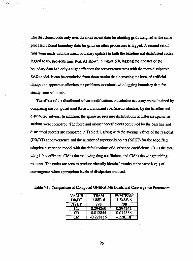
The distributed code only uses the most recent data for abutting grids assigned to the same

processor. Zonal boundary data for grids on other processors is lagged. A second set of

runs were made with the zonal boundary updates in both the baseline and distributed codes

lagged to the previous time step. As shown in Figure 5.8, lagging the updates of the

boundary data had only a slight effect on the convergence rates with the more dissipative

SAD model It can be concluded from these results that increasing the level of artificial

dissipation appears to alleviate the problems associated with lagging boundary data for

steady state solutions.

The effect of the distributed solver modifications on solution accuracy were obtained by

comparing the computed total force and moment coefficients obtained by the baseline and

distributed solvers. In addition, the spanwise pressure distributions at different spanwise

stations were compared. The force and moment coefficients computed by the baseline and

distributed solvers are compared in Table 5.1. along with the average values of the residual

(DR/DT) at convergence and the number of supersonic points (NSUP) for the Modified

adaptive dissipation model with the default values of dissipation coefficients. CL is the total

wing lift coefficient, CM is the total wing drag coefficient, and CM is the wing pitching

moment The codes are seen to produce virtually identical results at the same levels of

convergence when appropriate levels of dissipation are used.

Table 5.1: Comparison of Computed ONERA M6 Loads and Convergence Parameters

VALUEDR/DTNSUP

CLCDCM

TEAM1.88E-6

7980.2942600.012855-0.228115

PVMTEAM1.548E-6

7980.2942620.012856-.228118

95

The chordwise pressure distributions at two span stations computed by the distributed

and baseline solvers are compared with experimental data in Figures 5.9 and 5.10.

The poor correlation with experimental data in die shock region is a result of the coarse grid

used in these tests. However, the pressure distributions generated by the two flow solver

are virtually identical.

Baseline TEAMPVM TEAMExp. • Y/B = 0.44

Rgure 5,9: ONERA M6 Surface Pressure Distributions at 50% Span

96

-2-

1-1.5-E-o

Baseline Team• PVM TEAM

- •- - EXP - Y/B = 0.65

0.2 0.4 0.6 0.8

O

Figure 5.10: ONERA M6 Surface Pressure Distributions at 70% Span

5.1.3 Lockheed/AFOSR Wing C

A third set of Euler analyses were conducted using a seven block grid system for the

Lockheed/AFOSR Wing C geometry [127] supplied by the Lockheed Aeronautical Systems

Company. Wing C has an aspect ratio of 2.6, a taper ratio of 0.3, and a leading edge sweep

angle of 45 degrees. The Wing C geometry is a standard test case used in CFD validation

studies [3]. The Lockheed Wing C Euler grid system contains a total of 179309 nodes and

156672 cells. The wing planform and symmetry plane grids are shown in Figures 5.11 and

5.12.

97

Rgure 5.11: Wing C Symmetry Plane Grid

98

Figure 5.12: Wing CPIanfonn Grid

99

The grid has a C-O topology. The total number of points in each zone is shown in Figure

5.13. The largest of the seven zones contains 58695 nodes and the smallest zone contains

9867 nodes. Euler solutions were generated on both the HP and DEC systems for a Mach

number of 0.89 and an angle of attack of 5 degrees. All cases were run for 1000 steps.

Wing C - invlscld Grid |

Figure 5.13: Wing C Euler Grid Zonal Point Distribution

The HP systems consisted of the three machines used previously along with a faster

model 735 system. The Manager and one Worker process ran on the 735 system. The load

balance in terms of total grid points per processor was as follows: 29522 points and 38012

points on the Model 720 systems, 54080 points on the Model 730, and 58695 on the model

735. This distribution was chosen to fit each grid into the memory available on each

system. Four processors were used on the DEC systems with the Manager and the three

Worker processes on separate systems. For the distributed runs on the DEC systems, the

100

ad hoc load balance on the three Worker processes was 66534,54080, and 58695 points.

All cases were run for 1000 steps. A set of initial runs were made on each system with both

the baseline and distributed codes. For these cases, turnaround performance of the

distributed code was worse than the baseline code. For example, on the HP system the

baseline code required 19620 seconds for 1000 steps and the distributed code required

29942 seconds. This performance degradation was traced to the heavy utilization of the

model 735 by another user which lead to excessive job swapping by the operation system.

A similar degradation in performance was encountered on the DEC system.

At this point in the research, the Task Queue load balancing procedure was

implemented to attempt to minimize the effects of system utilization and load imbalance.

Because of the heavy utilization on the HP system, the initial tests of the Task Queue load

balancing procedure was performed on the DEC system. A series of runs were made to

determine the maximum and minimum performance of the distributed solver on the DEC

systems using roughly equal ad hoc load balance and the balance obtained by the Task

Queue approach. The maximum and minimum turnaround times in seconds for the baseline

code running on a single processor, the ad hoc approach, and the Task Queue approach are

given in Figure 5.14. The best time obtained for the baseline code was 21060 seconds.

With the ad hoc approach, the minimum time obtained was 14100 seconds and the

maximum time obtained was 23430 seconds. The minimum time represents a speedup of

1.49. For the Task Queue, approach the minimum time was 16410 seconds and the

maximum time was 27970 seconds. The minimum time for the Task Queue approach

represents a speedup of 1.28. The degradation in performance of the Task Queue approach

was due to the load balance obtained by the procedure. For the Task queue approach, the

distribution obtained on the three Workers was 84149,54080, and 41080 points. The

swapping introduced by the utilization of one of the Workers by another user led to the this

load distribution. This indicates that the procedure needs to be refined to optimize the load

101

'30000

EASELINE AD HOC TASK QUEUELOAD BALANCING SCHEME

Figure 5.14: Performance of Ad Hoc and Task Queue Load Balancing Schemes

distribution among the processors. The maximum and minimum times achieved with the

distributed code for both load balancing approaches again illustrate the sometimes drastic

effect that system load has on overall performance on an Ethernet based network system.

The minimum times were obtained in one of the few periods that all the worker processors

were either idle or very lightly loaded.

The tests with the initial version of the code validated the Manager-Worker strategy

used to implement the distributed solver and pointed out the need for an efficient load

balancing procedure. At this time, the focus of the research shifted to developing the

second version of the code using Version 713 of TEAM as the baseline code. This work

was performed at the NASA Ames Research Center on a system of SGI workstations.

102

5.2 Implementation and Validation of the Second Distributed

Solver

Based on the experience gained in die development of the first distributed solver, a

different approach was adopted for implementing the PVM modifications into the baseline

code to form the distributed solver. All modifications for the distributed solver were

implemented into the baseline code using the C language preprocessor and the UNIX make

utility to turn appropriate code segments on and off. This allowed a single code base to be

maintained instead of the two separate sets of source files used in the first solver. In

addition, the calls to the PVM library routines were embedded in wrapper subroutines that

acted as an interface between the baseline routines and the PVM routines. The second

version of the code was used to compare the performance of the Crutchfield static load

balancing procedure and as the basis for implementing the implicit LU-SGS algorithm.

The distributed network used for these tests was the RFA cluster of SGI workstations in

the NAS facility at the NASA Ames Research Center. The majority of the runs performed

in these tests were made using systems of three or five 75 megahertz Indigo 2 systems for

the Worker processes and a 50 Megahertz system for the Manager.

5.2.1 Comparison of the Performance of the Load Balancing Procedures

After the second implementation of the distributed solver was debugged, a series of

runs were made to compare the performance of the two different load balancing

approaches. The Wing C geometry for Euler simulations provided by Lockheed was used

for these tests. All solutions were run for 500 time steps using the Flux Adaptive

Dissipation (FAD) dissipation model with a second order dissipation coefficient of 0.1 and

a fourth order coefficient of 1.5 and the fourth order Runge-Kutta explicit solver. Tests

using three Worker processors were run first These were followed by runs using five

103

Worker processes. The baseline code was run on a single processor to provide the baseline

time used to compute the speed up. The best elapsed run time obtained for the single grid

case was 16500 seconds.

Representative speedups obtained by the two load balancing schemes are shown in

Figure 5.15. The static balancing approach required 12559 seconds for three Worker

processors and 13860 seconds for five Worker processors. The Task Queue approach

required 12844 seconds for three Worker processors and 11893 seconds for five Worker

processors. The performance degradation for the static balancing five processor case was

traced to a combination of the load imbalance obtained by the scheme and the extra systems

and communications overhead required by the additional processors.

PROCESSORS

Figure 5.15: Comparison of Speedup for Static and Task Queue Balancing SGI Systems

104

The load balances obtained by the two schemes are shown in Figures 5.16 and 5.17.

The improvement in performance obtained by the Task Queue procedure for the five

Worker case is felt to be primarily due to the more favorable balance obtained by the

procedure and a reduced level of system overhead. It was concluded from these tests that

both schemes perform about the same on lightly loaded systems. The Task Queue approach

has a slight advantage for networks with random system loads because it incorporates some

of the effects of system and network load into the load balance.

g80000STATICTASK QUEUE

PROCESSORS

Figure 5.16: Static and Task Queue Load Balance for Three Processors

105

1 . 2 3 4 5PROCESSORS

Figure 5.17: Static and Task Queue Load Balances for Five Processors

5.2.2 Implementation of the Implicit Solver

The next phase in the development of the second version of the solver was the

implementation of the LU-SGS implicit solver. After a series of tests to debug the coding, a

single processor case run using the inviscid Wing C case to obtain the turnaround

performance of the baseline code. The best time obtained was 12000 seconds. This

represents a substantial improvement over the 16500 seconds required by the Runge-Kutta

scheme. This improvement is due to die reduced computational effort of the implicit scheme

at each time step. The explicit scheme requires four flux evaluations and extra dissipation

evaluations for each step. The implicit scheme only requires one flux evaluation and one

dissipation evaluation per step. This offsets the computational effort required to compute

the flux Jacobians. The distributed version of the implicit solver was run using the static

106

load balancing procedure. The best elapsed time for the distributed solver was 6281

seconds using three Workers which represents a speed up of 1.91. The load balance for

this case was the same as the three processor Runge-Kutta case. The speed up for die three

processor Runge-Kutta case with static balancing was 1.3.

The variation in code performance obtained on the network based systems illustrates the

problems that can be encountered when running on Ethernet based systems. In addition to

the load balance dictated by the grid system used in the analyses, the systems and

communications load were found to play a substantial role in overall code performance.

This variation in performance and the limited availability of a sufficient number of

workstations led to the development of a third version of the flow solver on the large scale

IBM SP2 distributed supercomputing system at NASA Ames Research Center.

107

CHAPTER VI

STEADY AND UNSTEADY SIMULATIONS ON THE NAS SP2

A series of steady and unsteady simulations were performed on the IBM SP2 system at

the NASA Ames Research Center NAS facility. The NAS SP2 system is a large scale

distributed system placed at NASA Ames by IBM as part of the High Performance

Computing and Communications Program [128]. The SP2 system at the NAS facility is

composed of 160 processors or "nodes" connected with a high speed communications

subsystem [129]. Each node is an off-the-shelf IBM 590 workstation with a clock speed of

66.7 megahertz and a peak floating point speed of 250 megaflops per second All the nodes

on the NAS SP2 system have at least 128 megabytes of memory. The NAS SP2 system is

representative of the current state-of-the art in large scale distributed parallel systems based

on workstation technology.

The second version of the distributed flow solver was used for all the simulations

performed on the SP2. Initial steady flow simulations were made to validate the implicit

version of the code and to compare its performance to the explicit code. These tests were

made using the inviscid Wing C case provided by Lockheed. In addition, thin layer Navier-

Stokes simulations were performed using a large viscous grid system supplied by

Lockheed.

Unsteady flow simulations were performed for the FS wing geometry [130,131] using

the implicit version of the solver. For the unsteady simulations, the modal motion of the

wing oscillating in pitch was modeled. A series of tests were performed to determine the

108

effect of the domain decompositions used with increasing number of processors on the time

accuracy of the solution. These tests were also used to compare the performance of die

Manager/Worker and Worker/Worker communications strategies. In addition to die

unsteady simulations, a series of steady flow simulations were performed with die FS

geometry to determine die effect of die size of die fixed time step on solution accuracy and

convergence.

6.1 Wing C Euler Simulations

The previously described seven zone inviscid Wing C geometry and test case was run

using die Manager/Worker communications strategy. The principle objectives of these tests

were to continue the validation of die implicit algorithm and to compare its accuracy and

performance with results from die explicit scheme. As before, die Mach number and angle

of attack for these cases were 0.83 and 5 degrees. These runs were made using die

Modified Adaptive Dissipation model with die default dissipation coefficients. Load

balancing was performed using die static load balancing algorithm. Solutions were run for

400 steps with both die implicit and explicit schemes using systems of three, five and seven

SP2 nodes. The load balances for die three and five processor cases were die same as those

shown in Figures 5.16 and 5.17 for static balancing. For die seven processor case, each

zone was assigned to a different processor. The implicit scheme was run using die infinite

time step mode. The explicit scheme was run with a CFL number of 6. The run lengths

were limited to 400 steps so that single processor tests could be performed in die time limits

set for interactive jobs on die SP2 system diat were in place when these cases were run.

For these tests, die zonal boundary updates in die implicit scheme are lagged to die

previous time step when more than one grid is assigned to a processor. Local updates are

used in die explicit solver runs.

109

The turnaround times for the explicit and implicit versions of the baseline and

distributed codes using one, three, five, and seven processors are compared in Figure 6.1.

5000

0 2000

oc 1000

1 3 5 7NO. OF PROCESSORS

Figure 6.1: Comparison of Turnaround Peformance For The Explicit and Implicit Solvers

The explicit scheme required 4341 seconds for 400 steps on a single processor. The

distributed code required 1962 seconds with three processors, 1610 seconds with five

processors, and 1627 seconds with seven processors for the explicit scheme. The implicit

scheme required 3151 seconds on a single processor, 1555 seconds for three processors,

1227 processors for five processors, and 1167 seconds for seven processors. The

improved performance of the implicit scheme is felt to be due to several factors. The

primary difference is due to die fact that the implicit scheme is more efficient than die

explicit scheme because of the decreased number of flux and dissipation evaluations

required during each step. The improvements in performance obtained with increasing

110

numbers of processors was not expected due to die load imbalance of the five and seven

processor cases. This is felt to be due to the reduction in die largest load assigned to a

single processor and the smaller message sizes that must be routed through the Manager at

each step. This leads to a reduction in the time spent by the PVM routines in setting up and

transmitting die messages to each processor and in die idle time spent by me processors

with smaller loads as tiiey wait for die most loaded processor to finish. Even diough more

messages are being sent, the latency period for transmitting and receiving die messages is

less. This in turn leads to less idle time on each processor.

The relative speedups for both schemes are shown in Figure 6.2. The maximum speed

up of the explicit scheme occurs with five processors and has a value of approximately

2.69. The implicit scheme obtains a maximum speedup of 2.7 with seven processors.

3.0

2.5

£2.0

E 1-5UJ0)^ 1.0

§0.5QUJ

0.0

RK4-A- -LU-SGS

2 3 4 5 6 7NO. OF PROCESSORS

8

Figure 62: Comparison of Explicit and Implicit Scheme Speedups

111

Figures 6.1 and 6.2 illustrate the effect of load imbalance on speed up with increasing

numbers of processors. An equal load on each processor would lead to improved

performance. In addition, these results illustrate the advantage of a distributed system with

a switched high speed communications subsystem over the Ethernet based distributed

systems used in die first phase of the research. The maximum speedups of 2.7 approach

the ideal speedup of approximately 3.05 which assumes mat all communications are

instantaneous.

The total wing lift, drag, and pitching moments (CL, CD, and CM) along with the

number of supersonic points and the average change in density with time is shown in Table

6.1 for the implicit and explicit schemes.

Table 6.1: Total Wing Load Coefficients and Convergence Data on Different ProcessorsFor the Explicit and Implicit Solvers

VALUECLCDCM

NSUPDR/DTL2(l)

RK/1P0.5607773.9198E-2-0.134185

13,0111.195E-22.584E-5

RK/3P0.56078

3.9197E-2-0.134817

13,0061.202E-22.553E-5

RK/5P0.5607293.9179E-2-0.1347513,014

1.227E-22.590E-2

RK/7P0.5607453.9183E-2-0.134765

13,0121.225E-22.549E-2

LU / 1-7P0.55533

3.8764E-2-0.134475

12,8873.4393E-22.425E-6

The results for the explicit solver indicate mat the domain decomposition and modified

boundary update procedure has only a slight effect on computed loads. The computed

values for the implicit scheme do not change with increasing numbers of processors

because of the globally lagged boundary updates. No spatially varying time step was used

in the implicit calculations. However, a spatially varying step was calculated using a CFL

number of 6 to provide a consistent value of time step for computing the average change in

112

density with time. The code was modified to compute a second convergence parameter, the

Root Mean Square (RMS) average norm of the residual of die continuity equation. This

parameter is scaled to remove the effects of time step from the right hand side of the

discretized equations. The average norm is given by

where R(l) is the residual of the continuity equation and NC is the number of interior cells.

The values of L2(l) are also given in Table 6.1.

The differences in the loads and number of supersonic points computed by the implicit

and explicit schemes indicates that the two schemes are converging at different rates. A

second set of runs were made to quantify the effect of levels of convergence on the loads

computed by the two schemes. Five processors were used for these tests. The explicit and

implicit schemes were first run for 1400 steps. At this point an examination of the change

in the number of supersonic points at each step showed that the explicit scheme was almost

converged. However, the implicit scheme showed a small but noticeable oscillation in the

number of supersonic points at the end of 1400 steps which indicated that a steady state had

not been reached. The implicit scheme required another 600 steps to achieve the same level

of convergence as the explicit scheme. The force and moment coefficients computed by the

explicit and implicit schemes along with the number of supersonic points and the time

required for each solution are given in Table 6.2. After 2000 steps, tile number of

supersonic points computed by the two schemes are the same. The lift coefficients vary by

one count where a count is an increment of 0.0001. The drag and pitching moment

coefficients are seen to vary by less than a count These results indicate that the explicit and

113

implicit schemes will produce the same results for converged solutions. On an elapsed time

per step basis, the implicit scheme is more efficient However, the time required to achieve

similar levels of convergence is about the same.

Table 6.2: Computed Load and Convergence Data for the Explicit and Implicit Schemes

After 1400 and 2000 Steps

VALUE

CLCDCM

NSUPTIME(SEC)

RK/1400STEPS

0.5581870.039248-0.1367612,9935076

LU/1400STEPS

0.5581800.039198-0.1365613,0123969

LU/2000STEPS

0.5580830.039245-0.1367212,9935666

The results of the Euler tests indicated that both the explicit and implicit versions of the

distributed solver provided acceptable performance and accuracy for inviscid simulations.

The next step in die research was to validate the implicit and explicit solvers for viscous

simulations.

6.2 Wing C Viscous Simulations

A seven zone viscous grid for the Wing C geometry was obtained from Lockheed. This

grid system has a total of 479343 nodes and has a C-O topology. This grid system is

representative of the computational grids used in industry to validate Navier-Stokes

solvers. The number of points in each zone is shown in Figure 6.3. The largest zone in the

grid system contains 111725 points.

114

120000

2100000gu. 80000O

£ 60000CD

2 40000

< 20000

Figure 6.3: Grid Point Distribution for the Viscous Wing C Grid

A standard test case for the viscous grid system was also obtained from Lockheed. As in

the inviscid case, the viscous case was run with a freeestream Mach number of 0.85 and an

angle-of-attack of 5 degrees. The thin-layer approximation to the Navier-Stokes equations

was used to model the viscous stresses. The Baldwin-Lomax turbulence model was used

with transition fixed at constant chordwise stations along the span. The distributed viscous

Wing C tests were run using 5 processors. The load balance obtained by the static

balancing scheme is shown in Figure 6.4.

115

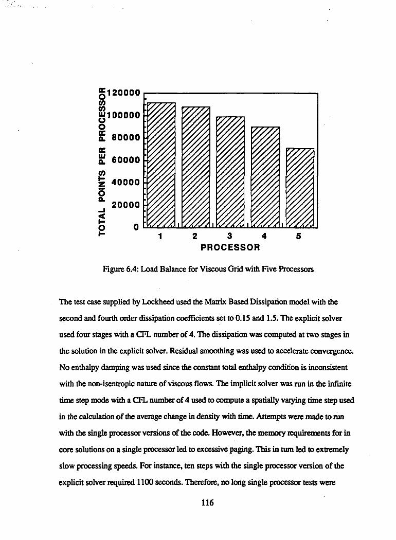
§120000(0U100000Oa 80000c£ 60000

40000

20000

1 2 3 4 5PROCESSOR

Figure 6.4: Load Balance for Viscous Grid with Five Processors

The test case supplied by Lockheed used the Matrix Based Dissipation model with the

second and fourth order dissipation coefficients set to 0.15 and 1.5. The explicit solver

used four stages with a CFL number of 4. The dissipation was computed at two stages in

the solution in the explicit solver. Residual smoothing was used to accelerate convergence.

No enthalpy damping was used since die constant total enthalpy condition is inconsistent

with the non-isentropic nature of viscous flows. The implicit solver was run in the infinite

time step mode with a CFL number of 4 used to compute a spatially varying time step used

in the calculation of die average change in density with time. Attempts were made to run

with the single processor versions of the code. However, the memory requirements for in

core solutions on a single processor led to excessive paging. This in turn led to extremely

slow processing speeds. For instance, ten steps with the single processor version of the

explicit solver required 1100 seconds. Therefore, no long single processor tests were

116

made. However, both the implicit and explicit versions of the distributed code were run for

2000 steps using die Manager/Worker communications strategy. This illustrates another

important advantage of distributed systems based on workstation technology. Large

problems can be broken into smaller problems mat can easily fit in the available memory of

each processor.

The initial distributed tests using the values of the dissipation coefficients supplied by

Lockheed produced solutions with stalled convergence rates. The average of the change in

density with time for the supplied dissipation coefficients are shown in Figure 6.5.

103

10*

c

<10°

LU-SGS-RK4

500 1000 1500 2000TIME STEP/ITERATION

2500

Figure 6.5: Convergence of Explicit and Implicit Schemes With Initial Dissipation Values

A second set of runs were made with the magnitudes of the second and fourth order•

dissipation coefficients increased to 0.5 and 2.0. The increased levels of dissipation

resulted in the improved convergence rates shown in Figure 6.6.

117

LU-SGS

-RK4

0 500 1000 1500 2000 2500TIME STEP/ITERATION

Figure 6,6: Convergence of Explicit and Implicit Schemes With Increased Dissipation

For this viscous case, the LU-SGS scheme required 16940 seconds and the RK4 scheme

required 25823 seconds to obtain approximately the same level of convergence. The

computed lift and drag coefficients along with the number of supersonic points obtained by

the two solvers are given in Table 6.3.

Table 6.3: Comparison of Total Loads and Convergence Data for the ViscousWing C Case Using the Explicit and Implicit Solvers

VALUECLCD

NSUP

RK40.546500.04546736,885

LU - SGS0.5501680.04579639,640

118

The implicit scheme produced a lift coefficient of 0.5502 and a drag coefficient of

0.045796 at the end of 2000 steps. This compares well with a lift coefficient of 0.5465 and

a drag coefficient of .045467 produced by the explicit scheme.

The viscous Wing C tests validated the performance of the distributed versions of the

explicit and implicit solvers for steady viscous simulations. The next phase of the research

examined the performance of the implicit solver for unsteady flow simulations. The explicit

solver was not used for these tests because of its increased computational requirements and

the prohibitively small time steps that would be required to maintain stability.

6.3 F5 Wing Simulations

A series of simulations were performed using the F5 wing geometry to determine the

effectiveness of the implicit version of the distributed flow solver for unsteady flow

simulations. The primary goal of these tests was to determine the effect of the boundary

update procedure required by the distributed solver on solution accuracy for an oscillating

wing. Results were generated for the modal vibration of the F5 wing oscillating in pitch

and compared with the experimental results of Tijdeman et al. [131]. The experiments of

Tijdeman et aL have been used by several authors to validate different computational

methods for unsteady flow analysis [132-140]. The performance of the Manager/Worker

and the Worker/Worker communication strategies was evaluated for distributed systems of

up to 18 processors. In additions, steady simulations were performed to determine the

effect of time step size on solution accuracy and performance.

119

6.3.1 F5 Wing Test Configuration

The test configuration used in the experiments of Tijdeman et aL is shown in Figure

6.7. In the unsteady experiments, the wing was subjected to a sinusoidal oscillation in pitch

about the half chord location of the root section. The unsteady pressures and the modal

response of the wing were measured for a range of Mach numbers, mean angles of attacks,

and frequencies of oscillations.

10

DISPLACEMENTTRANSDUCER

>=>

O PRESSURE ORIFICE• M4-SITU TRANSDUCER• ACCELEROMETERB MINCE

Figure 6.7: FS Experimental Test Configuration (Reference 130)

120

The spanwise locations where pressures were measured are given in Table 6.4.

Table 6.4: Spanwise Locations of Experimental Pressure Datafor the F5 Wing

Station No.12345678

y/b(%)18.135.251.264.172.181.787.597.7

The modal response of the wing was obtained by integrating the local accelerations

obtained from the accelerometers measured on the wing. An analytical function for the

mode shape of the wing was obtained by integrating the accelerometer data twice. This

analytical mode function combines both the bending and torsion modes of vibration that

occur on swept and tapered wings such as the F5 wing. The experimental test case used in

the present research had a freestream Mach number of 0.896, a mean angle of attack of 0

degrees, an amplitude of oscillation of 0.111 degrees, and a frequency of oscillation about

the root half chord location of 40 Hertz. The freestream Reynolds number for this test

condition was 11 million based on root chord. The F5 wing model used in the experiments

has a root chord of 0.6396 meters and a span of 0.6226 meters. The leading edge sweep

angle is approximately 32 degrees.

The mode shape function obtained by Tijdeman et al. for the chosen test case is given

in Reference [131] as

121

W(x,y) = -0.329 -I- 0.977x - 0.088y + 0.244xy - O.OVTy2 - O.Wlxy2 (6.2)

where x is the chordwise ordinate and y is Ac spanwise ordinate. The procedures used to

generate Equation (6.2) assumed there was no chordwise deformation and a parabolic

spanwise deformation. In addition, Equation (6.2) is nondimensionalized such mat the

tangent of the angle of oscillation at the second experimental span station is equal to one.

In the current research, Equation (6.2) is used to define an angular displacement about

the chordwise position at each span station at which the angular displacement given by the

equation is zero. The spanwise locus of the chordwise positions of zero displacement

define the node line for the wing. The modal motion of the wing is assumed to consist of a

rigid rotation about the node line. The mean sinusoidal motion of the wing is defined by

ot(t) = cto + Aa sin(w) (6.3)

where a(t) is the instantaneous angle of attack at time t, OQ is the mean angle of attack, Aa

is the amplitude of oscillation, and K is the reduced frequency defined as

(6.4)

where F is the frequency in Hertz, c is a reference chord length and U is the freestream

velocity. In the experiments of Tijdeman et aL, the reduced frequency is defined such that

the value given in the Reference [131] is half die value computed by Equation (6.4). For a

frequency of oscillation of 40 Hz and a freestream Mach number of 0.896, the reduced

122

frequency given by Tijdeman et aL is 0.275. The value of reduced frequency used in this

research is the value given by Equation (6.4) using the root chord as the reference length.

The local angular displacement at a constant span station can be defined in terms of the

instantaneous mean sinusoidal motion of the wing given by Equation (6.3 and the mode

shape given by Equation (6.2) as

a(y,t) = 6(y)a(t) (6.5)

where 9(y) is the mode shape at each span station based on a rigid rotation about the

chordwise location of the local node. In the computational results, Equation (6.5) is applied

to the two-dimensional grid planes defined at constant spanwise stations. The rotation of

the grid planes are first performed about the node line. These rotations are then transformed

to rotations about the root half chord location.

6.3.2 Computational Grid System

The grid system for the computational tests were generated analytically using the

procedure used by Guraswamy [138] in the ENS AERO code. Two dimensional grids are

generated at each spanwise location by marching outward from the inner boundary defined

by the wing and wake surfaces to a fixed outer boundary distance along directions defined

by the outward unit normal vectors at each point on the inner boundary. Stretching

functions defined in the coordinate direction approximately normal to the inner boundary

are used to define the increments in the x and z directions that are added to the coordinates

of the previous coordinate surface to define the coordinates on successive surfaces. The y

coordinate of each grid plane is held constant

123

The grid generation procedure was used to generate a baseline C-H mesh system

consisting of 151 strcamwise points, 28 spanwise points with 19 or 20 points on die wing

surface and 45 normal points. There are total of 190,260 points in the grid. There are 101

points on the body surface at each spanwise station. The region outboard of the wing tip

and the wake surfaces aft of the wing trailing edge are modeled as a fluid surfaces of zero

thickness. The initial grid normal grid spacing for Euler simulations was set at 0.001 root

chords. The normal grid spacing for viscous simulations was set at 0.00002 root chords.

Analytical stretching functions were used to cluster the grid in the normal directions and

chordwise directions. This grid system was chosen to facilitate comparisons with results

reported in References [136] and [137]. The symmetry plane and wing planform grid

systems are shown in Figure 6.8.

Figure 6.8 F5 Planform and Symmetry Plane Grids

124

For the distributed simulations, the grid was subdivided into 4,9, and 18 zones with

each zone containing the same number of points to maintain an equal load balance among

processors. The 9 and 18 zone cases contained four spanwise stations in each zone and the

4 zone case contained 8 spanwise stations in each zone. The 18 zone system was obtained

by splitting the 9 zone system in the normal direction. These grids were used to evaluate the

performance of both die Manager/Worker and Worker/Worker communications strategies

and to determine the effects of die domain decomposition on solution accuracy.

6.3.3 Results of Unsteady Simulations

A series of Euler and Navier-Stokes analyses were performed using the baseline C-H

mesh. Euler simulations using the four zone grid system were performed first All

simulations were run for three cycles of oscillation with 1621 steps per cycle for a total of

4863 steps. This corresponds to a non-dimensional time step of approximately 0.005. The

choice of this step size is based on the results of Mello [140] for the same test case. As in

Reference [140], the reduced frequency used in the calculation of time step and the motion

of the wing was redefined in terms of the freestream Mach number and a reference chord

length of one meter to give consistent values for the non-dimensional parameters used in

the flow solvers. The Matrix Based Dissipation model was used in these tests. This is

equivalent to using an upwind biased scheme.

The unsteady pressure response for the oscillating wing is a complex function that can

be broken into real and imaginary components [140]. The real and imaginary pressure

coefficients are defined in terms of the instantaneous values of pressure coefficient at each

time step by Fourier integrals of the form

125

CPreal =

CpI,+2* /M.K

unag7C

(6.6a)

(6.6b)

where the initial non-dimensional time t, is chosen to be large enough such that transients

that appear in the initial phases of the solution have disappeared The integrals are over the

time period required for one complete cycle of motion. The real values components of the

unsteady coefficients represent the components that are in phase with the prescribed

motion. The imaginary components are out of phase with the motion.

The actual evaluation of the integrals in Equations (6.6) is performed by trapezoidal

integration. In addition, the final values of the coefficients are scaled by the amplitude of

oscillation in radians, Act. This scaling was used in the experimental results. The

discretized equations for the unsteady coefficients can be written as

m=ms+l(6.7a)

rcAaCp(n.sHCp(mE) +

mp-

m=ms+l(6.7b)

where n^ and mE are the indices of the time steps at the start and end of the cycle over

which the integrals are evaluated. Cp(m) is die pressure coefficient at a point on the wing

126

surface for time step m. For the unsteady simulations performed in this research, the real

and imaginary pressure coefficients were computed over the third cycle of oscillation.

6.3.3.1 Unsteady Euler Simulations

The computed real and imaginary upper surface pressure coefficients for the four zone/

four processor Euler analysis are compared with digitized experimental data from Reference

[131] in Figure 6.9 at spanwise computational grid locations of 35%, 51%, and 88%. The

semispan locations of the experimental data are 352%, 51.2%, and 87.5%. The computed

results presented in Figure 6.9 are in good agreement with both the experimental results

and the computational results presented in References [136] and [137]. At the inner wing

stations, the correlation of the computed real (in-phase) components of pressure with the

experimental data is excellent The computed shock location in imaginary (out-of-phase)

component is slightly downstream of the experimental data. At the outboard wing station,

the correlation for the real component shows a shock wave that is upstream of the

experimental results and slightly stronger. However, the peak is consistent with the results

obtained by Obayashi et al. [136] using an upwind biased scheme. The correlation of the

computed imaginary component of the pressure coefficient with the experiment is very

good. On the whole, the computed results are in excellent agreement with the experimental

data. It should be noted that the differences in the results are magnified by the pitch

amplitude seating used in both the computed and experimental data. An increment of one in

the scaled data corresponds to a change of 0.002 in the actual data. Other differences can be

attributed to viscous effects in the outboard region and inconsistencies in the experimental

data. These results indicate the implicit scheme provides sufficient time accuracy for the 4

zone / 4 processor Euler simulations for a time step of 0.005. The turnaround performance

127

-10

-5

o.O_ 0a£

10

Real Cp • 4Z/4P• Real Cp (Upper) • Exp

i ... i0.2 0.4 0.6 0.8 1

X/C

(a) Upper Surface Real Pressure Coefficient at 35% Span

•10

-5

aOO)a

10

Imag Cp - 4Z/4P• Imag Cp (Upper) - Exp

i ... i0 0.2 0.4 0.6 0.8 1

X/C

(b) Upper Surface Imaginary Pressure Coefficient at 35% Span

Figure 6.9: Four Processor Real and Imaginary Pressure Distributions for the

For the Inviscid F5 Wing Case, M=0.9, F=40Hz.

128

•10

ao_ oSoc

10

Real Cp • 4Z/4PReal Cp (Upper) • Exp.

0.2 0.4 0.6 0.8X/C

(c) Upper Surface Real Pressure Coefficient at 51% Span

-10

-5

aaO)CO

10

Imag Cp - 4Z/4P• Imag Cp (Upper) - Exp.

0.2 0.4 0.6 0.8 1X/C

(d) Upper Surface Imaginary Pressure Coefficient at 51% Span

Figure 6.9: Four Processor Real and Imaginary Pressure Distributions for the

Inviscid F5 Wing Case, M=0.9, F=40Hz (continued).

129

-10

-5

a° 0Soc

5

10

Real Cp - 4Z/4P• Real Cp (Upper) » Exp

0.2 0.4 0.6 0.8x/c

(e) Upper Surface Real Pressure Coefficient at 88% Span

-10

-5

Q.oo>a

10

Imag Cp - 4Z/4PImag Cp (Upper) • Exp

0.2 0.4 0.6X/C

0.8

(f) Upper Surface Imaginary Pressure Coefficient at 88% Span

Figure 6.9: Four Processor Real and Imaginary Pressure Distributions for the

Inviscid F5 Wing Case, M=0.9, F=40Hz (concluded).

130

for this case on the SP2 using the Manager/Worker communications strategy was 18174

seconds.

Next, the 9 zone / 9 processor and 18 zone /18 processor cases were run to determine

how turnaround performance scales with increasing number of processors and the effect of

the domain decomposition on the accuracy of the implicit scheme. Both die 9 zone and

eighteen zone grid systems were purposely limited to a maximum of 4 spanwise grid planes

per zone. This makes the solution in each zone almost two-dimensional. In addition, the

dissipation can no longer be evaluated at all the interior planes using a five point stencil.

The object was to determine the lower bound for the spanwise domain decomposition that

would maintain an accurate solution. The real and imaginary upper surface pressures

obtained at the 33% and 88.5% of span stations for the 9 and 18 zone cases are compared

with the results for the four zone case obtained at the 35% and 88% span stations in Figure

6.10. The difference in the location of the span stations is due to the introduction of an

additional grid plane to maintain an even load balance. Reducing the number of spanwise

grid planes per block from eight to four is seen to have a slight effect on accuracy at the

inboard station. Differences are more pronounced at the outboard station. These differences

can be attributed to the loss of implicitness in the solution due to the decreased number of

131

-10

10

Raal Cp • 4 Zon««/Proc«D R»al Cp - 9 Zon»«/Proc»

• Real Cp - 18 Zonts/Proc*

0 0.2 0.4 0.6 0.8 1X/C

(a) Upper Surface Real Pressure Coefficient at 33% Span

-10

Imag Cp 4 Zonas/ProcsD Imag Cp 9 Zon«s/Procs

— — - Imag Cp - 18 Zones/Procs

0 0.2 0.4 0.6 0.8 1X/C

(b) Upper Surface Imaginary Pressure Coefficient at 33% Span

Figure 6.10: Comparison of 4,9, and 18 Processor Real and Imaginary Pressure

Distributions for the Inviscid F5 Wing Case, M=0.9, F=40Hz.

132

-10

10

Roil Cp - 4 Zonaa/ProcsO Raal Cp - 9 Zonaa/Proca

Roal Cp - 18 Zonaa/Proca

0.2 0.4 0.6 0.8 1X/C

(c) Upper Surface Real Pressure Coefficients at 88.5% Span

•10 r

Imag Cp - 4 Zones/ProcsD Imag Cp - 9 Zonaa/Proca

Imag Cp - 18 Zonaa/Proca

0 0.2 0.4 0.6 0.8 1X/C

(d) Upper Surface Imaginary Pressure Coefficients at 88.5% Span

Figure 6.10: Comparison of 4,9, and 18 Processor Real and Imaginary Pressure

Distributions for the Inviscid F5 Wing Case (concluded)

133

spanwise grid planes in each block. In addition, the reduced number of spanwise stations

in the transition region between the solid surface and the wake surface outboard of the tip

slows the evolution of the flow field around the wing tip. However, these results indicate

that acceptable accuracy can be maintained as the computational domain is decomposed into

smaller blocks.

It was noticed during die comparisons of the 4,9, and 18 zone cases that the speedup

in turnaround performance using the Manager/Worker strategy deteriorated with increasing

numbers of processors. The time required for the 18 zone case to go 4863 steps was 8984

seconds. This is only an improvement in performance of a factor of two over the 4 zone

case. This result prompted the implementation of the Worker/Worker communications

strategy. The turnaround performance of the Manager/Worker and Worker/Worker

strategies for the three grid systems is given in Figure 6.11.

20000

•016000o£12000

oI 8000

4000 MANAGER/WORKER— B- -WORKER/WORKER

0 5 10 15 20Zones/Processors

Figure 6.11: Comparison of Manager/Worker and Worker/Worker Performance

134

For a small number of processors, the Worker/Worker strategy is slightly faster than the

Manager/Worker scheme. The turnaround time for the Worker/Worker approach for 4

processors is 17670 seconds. The difference in the performance of the two schemes is seen

to increase substantially as the number of processors is increased For the nine processor

case, the Manager/Worker scheme required 11987 seconds for 4863 steps. In contrast, the

Worker/Worker scheme required 9671 seconds. The turnaround time for the 18 processor

Worker/Worker case is 4410 seconds. This is a relative speedup of a factor of 4 over the 4

processor case. The ideal speedup of the 18 zone case over the 4 zone case would be a

factor of 4.5.

The deterioration of the Manager/Worker strategy is due to the wait time imposed on the

Worker processes as the Manager collects and sends the required zonal boundary

information to and from each Worker. Because of the equal load balance, all the processors

are finishing at approximately the same time. Therefore, a bottleneck is formed as the

Manager sends and receives the data to and from each processor. The Worker/Worker

strategy removes this bottleneck by allowing the Workers to communicate directly with

each other. The time spent waiting to receive data is effectively cut in half as the number of

processors increases because the Workers do not have to wait on the Manager. These

results demonstrate the superiority of the Worker/Worker scheme for large scale systems

with high-speed communications subsystems.

6.3.3.2 Unsteady Viscous Simulations

A turbulent thin-layer Navier-Stokes simulation was performed using the 18 zone grid

system and the Matrix Based Dissipation Model The upper surface real and imaginary

pressure coefficients are compared with the inviscid results and the experimental data at the

33% and 88.5% span stations are shown in Figure 6.12. The viscous case was run with a

Reynolds number of 9 million. A free transition to turbulence was assumed. These results

show little or no improvement due to the incorporation of viscous effects in the correlation

135

-10

-5

Q.oI oS

10

Real Cp - InvR«al Cp -Vis

O Real Cp (Upper) • Exp.

0 0.2 0.4 0.6 0.8 1X/C

(a) Upper Surface Real Pressure Coefficient at 33% Span

-10

-5

a.OO)CO

10

Imag Cp • InvImag Cp • Vis

O Imag Cp (Upper) Exp.

i ... I

0.2 0.4 0.6X/C

0.8 1

(b) Upper Surface Imaginary Pressure Coefficient at 33% Span

Figure 6.12: Comparison of Viscous and Inviscid Pressure Distributions for

the F5 Wing Using Four Processors, M=0.9, F=40Hz.

136

-10

-5

a.o•a9

DC

10

Rail Cp • Inv— - R«al Cp • VI*O Real Cp (Uppar) • Exp

0.2 0.4 0.6 0.8 1x/c

(c) Upper Real Pressure Coefficient at 88.5% Span

-10

-5

o> 0

i

10

Imag Cp - InvImag Cp - Vis

O Imag Cp (Uppar) - Exp

i ... I

0 0.2 0.4 0.6 0.8 1X/C

(d) Upper Surface Imaginary Pressure Coefficient at 88.5% Span

Figure 6.12: Comparison of Viscous and Inviscid Pressure Distributions for

the F5 Wing Using Four Processors, M=0.9, F=40Hz.(concluded)

137

with the experimental results. This indicates that a more refined computational grid is

required for the viscous simulations. The transition locations should be fixed to the

experimental values. These simulations were performed to determine if the inclusion

viscous terms would yield a substantially different solution. The viscous case required

about 5800 seconds for 4863 steps with the Worker/Worker strategy.

6.3.4 Steady Flow Results

A series of steady thin-layer Navier-Stokes analyses were performed with the unsteady

implicit solver using two fixed time steps to determine the effect of the time step size on the

solution convergence properties. The analyses were run for the Mach 0.896 case at a

Reynolds number of 9 million using the 18 zone grid system. The non-dimensional time

steps used were 0.006 and 0.067. The smaller time step was run first for 3600 steps. The

large step size was run for 4000 steps. The average change in density with time and the

L2(l) average norm of the residual of the continuity equation is given if Figures 6.13 and

6.14 for both time steps. The data in Figure 6.13 was computed with the CFL number set

to 1.0. As would be expected, the solution appears to be converging faster for the larger

time step size. However, the comparison of the convergence of the number of supersonic

points given in Figure 6.15 shows that the large step achieves a steady state only a few

hundred steps sooner than the smaller step size.

The computed steady pressure distributions computed with the 0.067 time step are

compared with experimental results at the 33%, 53%, and 88.5% span stations in Figure

6.16. The computed lower surface pressure distributions are in excellent agreement with

the experimental results. The mismatch in upper surface shock position on the outboard

station can be attributed to the differences in the spanwise locations of die computational

and the experimental data, the effects of the turbulence model, and an inadequate number of

grid points in the normal direction. The time constraints on this research prevented a more

138

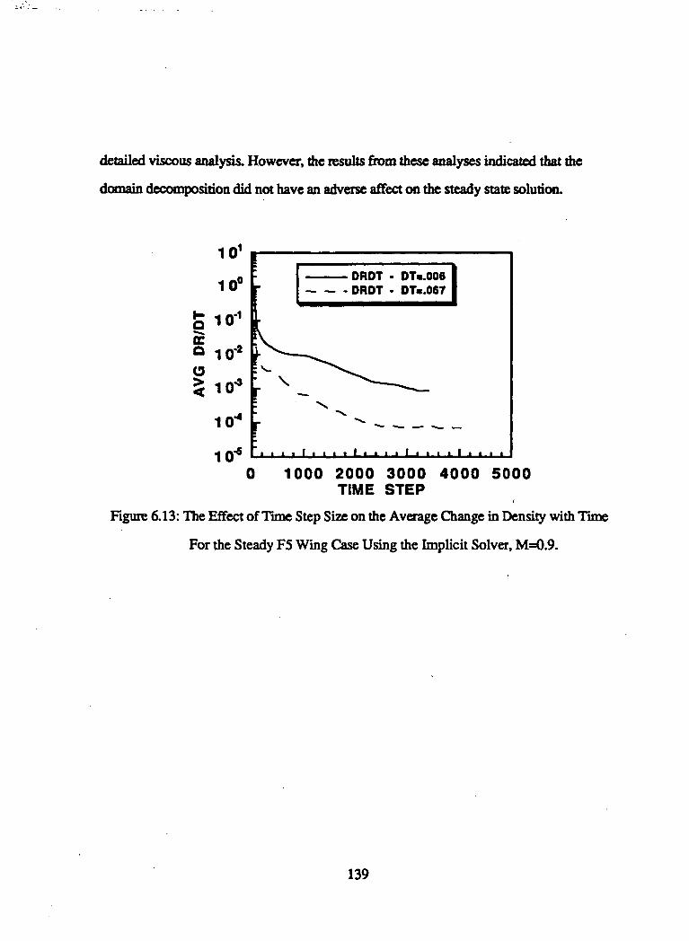
detailed viscous analysis. However, die results from these analyses indicated that the

domain decomposition did not have an adverse affect on the steady state solution.

10°

§ 10«o

10*

10*

DRDT - DT..006— - DRDT - DT..067

\

0 1000 2000 3000 4000 5000TIME STEP i

Figure 6.13: The Effect of Time Step Size on the Average Change in Density with Time

For the Steady F5 Wing Case Using the Implicit Solver, M=0.9.

139

10"

10"

10'7

10"

10"

L2 (RHS) - DT..006— -L2(RHS) . DT..067

0 1000 2000 3000 4000 5000TIME STEP

Figure 6.14: The Effect of Time Step Size on the L2 Norm of the Continuity Equation

for the Steady F5 Wing Case Using the Implicit Solver, M=0.9.

(012000

010000tL

NSUP • DTs.006-NSUP - DTs.067

0 1000 2000 3000 4000 5000TIME STEP

Figure 6.15: The Effect of Time Step Size on the Number of Supersonic Points

for the Steady F5 Wing Case Using the Implicit Solver, M=0.9.

140

•0.8

§ °'2

0.4

0.6

0.8

Cp • Lower— — - Cp • Upper

O Exp. • LowerD Exp. - Upper

0.2 0.4 0.6X/C

(a) 33% Span

0.8

o"o

1oO

£a0>2Q.

Q.O

-0.8

•0.6

-0.4

•0.2

0

0.2

0.4

0.6

0.8

Cp - Lower— — - Cp - Upper

O Exp. - LowerD Exp. • Upper

0.2 0.4 0.6X/C

0.8

(b) 53% Span

Figure 6.16: Steady Viscous Pressure Distributions for the F5 Wing, M=0.9

141

-0.8

2 0

S 0.220. 0.4

a 0.6O

0.8

Cp • LowerCp • Upper

O Exp. • LowerO Exp. • Upper

0.2 0.4 0.6X/C

0.8

(c) 88.5% Span

Rgure 6.16: Steady Viscous Pressure Distributions for the F5 Wing, M=0.9 (concluded)

142

CHAPTER VII

CONCLUSIONS AND RECOMMENDATIONS

In this research, explicit and implicit multi-acme three dimensional flow solvers were

successfully implemented to perform as parallel distributed flow solvers on two different

types of distributed computing systems using the PVM software interface. The first

distributed systems used were composed of small Ethernet based networks of engineering

workstations. A series of steady flow analyses on these systems validated the performance

of the initial explicit flow solver and demonstrated the need for effective communications

and load balancing strategies. Two different static load balancing approaches were

evaluated and shown to provide adequate performance on lightly loaded networks.

However, it was found that the performance of the network based solver was heavily

dependent on system load. The Manager/Worker scheme was found to be an effective

communications strategy for small network based systems. The utility of using the PVM

software system to nun an existing multi-zone flow solver into a distributed solver was

demonstrated. The results from the network based systems demonstrated that small scale

Ethernet systems can be used to provide acceptable turnaround for moderate problems.

The second distributed system used in this research was the large scale IBM SP2

distributed system that is part of NASA's Numerical Aerodynamics Simulation facility. The

performance of the original explicit solution algorithm and an implicit solver based on die

LU-SGS solution scheme of Yoon and Jameson was compared for both steady and

unsteady flow simulations. The steady flow simulations demonstrated the accuracy and

143

performance of the both distributed solvers for both inviscid and viscous simulations of the

Lockheed/AFOSR Wing C geometry.

Steady and unsteady flow simulations were performed for the F5 wing with the implicit

solver to investigate the effects of domain decomposition on solution accuracy. Unsteady

simulations were performed with distributed systems of up to eighteen processors. The

Worker/Worker communications strategy was successfully implemented to alleviate the

problems of performance degradation encounter with the Manager/Worker scheme for

increasing numbers of processors.

The results of the present research to develop efficient computational strategies for three

dimensional flow simulations on distributed systems have led to the following conclusions

and recommendations for future research.

7.1 Conclusions

The effectiveness of both networks of engineering workstations and large scale

distributed systems based on workstation technology for real world Computational Fluid

Dynamics simulations was demonstrated. The performance of distributed flow solvers is

dependent on the implementation of efficient communications and load balancing strategies.

It was found that Ethernet based systems can only be effective when the systems

comprising the distributed system are very lightly loaded and network communications

traffic is a minimum. A static load balancing procedure such as die Task Queue approach

or a fully dynamic balancing scheme that can incorporate some of the effects of system load

into the initial load balance is required for optimum performance on loaded systems. For

lightly loaded systems, die Crutchfield static balancing algorithm proved to be an effective

alternative to the Task Queue scheme.

144

The type and magnitude of numerical dissipation used in both the implicit and

distributed solvers was found to be an important factor in alleviating the adverse effects on

solution convergence that are introduced by the lag in the updating of zonal boundary

conditions that is inherent in the distributed solvers. Levels of dissipation that were

adequate for single processor solutions with the baseline explicit scheme were found to lead

to either a stall convergence rate or divergence when used with the distributed solver.

However, increasing die levels of fourth order dissipation was found to alleviate the

problem. With proper levels of dissipation, the distributed solvers were found to provide

the same accuracy as the baseline single processor solvers with greatly improved

turnaround time performance.

The distributed implicit solver based on the LU-SGS scheme was found to be a viable

alternative to the explicit solver for both inviscid and viscous simulations. For both Euler

and Navier-Stokes simulations, the implicit scheme was found to be computationally more

efficient on a time required per step basis than the explicit scheme. However, the time

required to reach a steady state solution was about the same for the Euler simulations

performed for the Wing C configuration.

The viability of an unsteady distributed solver based on the LU-SGS scheme was

demonstrated by the unsteady FS solutions. It was found that the computational domain

could be subdivided into relatively small units without a serious degradation in solution

accuracy. However, more research is required to quantify the effects of the lagged

boundary update procedure on the time accuracy of larger scale problems. The results of

the steady F5 analyses indicate that the effect of the domain decomposition on steady state

Solutions is alSO minimal.

TheManager/Worker strategy was found to be inadequate for systems such as the SP2

that utilize a switched high-speed communications subsystem. The Worker/Worker strategy

was found to deliver superior performance with increasing numbers of processors when

145

there is an equal load balance. However, no communications strategy can overcome the idle

time introduced by an unequal load balance. Therefore, effective procedures for domain

decomposition either prior to or during the solution are required to maintain the scaling of

turnaround performance that is expected with increasing numbers of processors.

Finally, it is felt that the computational approaches evaluated in this research provide a

useful knowledge base for the development of new distributed solvers or the extension of

existing multi-zone solvers for use on distributed systems.

7.2 Recommendations

The results and conclusions drawn from the present research have led to the following

recommendations for extensions of the distributed flow solvers and for future areas of

research:

1) A more detailed analysis needs to be made of the effects of the boundary update

procedures on the time accuracy of the solution for viscous simulations. This would require

the use of larger viscous grid systems than were used in the present research.

2) An alternate implicit scheme such as the diagonal scheme of Pulliam and Chausee

should be compared with the LU-SGS scheme for both steady and unsteady simulations.

In addition, the Newton iteration scheme should be implemented to increase die temporal

order of accuracy of the implicit schemes and reduce the effect of the boundary update

procedure on temporal accuracy. More work is required to quantify if the increased

computational effort required by the Newton iteration scheme is justified.

3) The current Manager/Worker code structure should be unified into a single code to

provide a Single Program Multiple Data (SPMD) version of the code. This would save a

processor on systems with a limited number of available processors.

146

4) A version of die distributed solver based on die Message Passing Interface (MPI)

should be implemented and its performance compared with the PVM versions of the solver.

5) A preprocessor should be developed that can decompose an existing unbalanced multi-

zone grid system into a more evenly balanced system. An alternate approach would be to

implement a dynamic load balancing algorithm that could generate evenly balanced

subdomains from the initial grid system.

Finally, it is hoped that the worked performed in the present research can serve as the

basis for the development of a production CFD code that can be a useful tool for

aerodynamic analyses and design.

147

APPENDIX A

THE BALDWIN-LOMAX TURBULENCE MODEL

«••

The Baldwin-Lomax turbulence model is a two-layer algebraic model based on a similar

model proposed by Cebeci and Smith [52]. Both models use the Bossinesq approximation

to compute a turbulent eddy viscosity, m-, that is combined with die molecular viscosity to

form an effective value used in the calculation of the viscous terms in the Navier-Stokes

equations. For wall bounded flows, the viscous region normal to the wall is assumed to be

composed of inner and outer layers with different length scales. Unlike the Cebeci-Smith

model which requires an explicit definition of the location of the edge of the boundary

layer, the Baldwin-Lomax model defines uses the distribution of vorticity normal to the

wall to define the length scales and corresponding eddy viscosities in the inner and outer

layers. The value of the eddy viscosity is switched from die inner layer value to the outer

layer value at the minimum normal distance from the wall where the inner and outer layer

values of eddy viscosity are equal, This point is called the crossover point, y^o^^er

In the inner layer, the eddy viscosity is defined by the Prandtl- Van Driest formulation

(A.D

where the length scale, I, is given by

148

* = Ky l-el ' ' (A.2)

In Equation (A.2), K is the von Karman constant which has a value of 0.4 and y is the

normal distance from the walL The term enclosed in brackets is the Van Driest damping

factor that goes to zero at the wall The parameter, y*, is a non-dimensional length that is

used in the law of the wall [48] to define the extent of the viscous sublayer where the

molecular viscosity dominates the flow, y* is obtained from the relation

(A3)

where pw, tw, and ̂ are the density, shear stress and molecular viscosity at the wall. The

parameter, A+, is a constant whose value is normally set to 26 which provides the correct

log-law profile near the wall for flow over a flat plate with zero pressure gradient [48] and

is consistent with Cebeci's [141] formulations for a constant pressure boundary layer at

transonic speeds. The magnitude of the vorticity is defined as

du (A-4)

In the outer layer, the eddy viscosity is defined as

149

(A-5)

where C,̂ is the Clauser constant whose value is 0.0168 and C^ is an empirically

derived constant with a standard value of 1.6. Fwike is given by

(A.6)

Values for the parameter F,,̂ are obtained from the maximum value of the function

(A.7)

evaluated normal to the wall, y^ is the y location at which F,^ occurs. The quantity,

Udjff, is defined by the difference in the magnitudes of the minimum and maximum

velocities in the boundary layer profile at a fixed station

(A.8)max ./mn

For wall bounded flows, the minimum velocity will occur at the solid surface and is zero

for steady flows because of the no-slip condition. The function, F^, is the Klebanoff

intemittency correction that accounts for the intermittent changes in the viscosity at the edge

of the boundary layer and is given by the relation

150

-r-1

(A.9)

In the free wake region behind a body such as a wing or an airfoil, the Baldwin-Lomax

model is modified by setting the exponential term in the function F(y) defined by Equation

(A.7) to zero. In the wake, the no-slip condition at the solid wall no longer in effect

Therefore, the minimum velocity used in Equation (A.8) must be specified.

Once the inner and outer values of the eddy viscosity are computed, the final values are

set using the conditions

innerf

> ycrossoverj(A.10)

151

APPENDIX B

THE INVISCID FLUX JACOBIAN MATRICES

The inviscid flux Jacobian matrices A, B, and C used in the implicit schemes can be

obtained by expanding the differential of the appropriate flux vector in a given coordinate

direction and using the relation

dQ(B.I)

Along any curvilinear coordinate surface £, T|, or £, the flux Jacobian can be defined by a

generic matrix of the form

A =

4>kx-uUn U-p2ukx uky-pvkx ukz-pwkx pkx

<|>ky-vUn vkx-puky U-p2vky vkz-pwky pky

<j)kz-wUn wkx-pukz wky-pvkz U-p2wkz _pkz

Hkx-puUn Hky-pvUn Hkz-pwUa U + pU,

(B.2)

where k is one of the general coordinates £, T), or £. The derivatives k,, k,» and k, can be

defined in terms of normalized metric quantities that make Equation (B.2) applicable for

152

both finite difference and finite volume formulations. For instance, for k=£, k, can be

written as

where Sx, Sy, and Sz are the Cartesian components of the area vector normal to surface k.

The parameters u, v, and w are the Cartesian components of velocity. H is the total

enthalpy per unit volume. The variables <J), P, and P2 are defined as

(B.4)

where 7 is the ratio of specific heats. The parameters k, and Un are the grid and flow

velocities normal to surface k and U is the contravariant velocity. These parameters are

defined by the relations

+ ztkz) , Un = ukx + vky + wkz , U = Un + kt (B.5)

where x, , y, and z, are the Cartesian grid speeds.

153

APPENDIX C

MANAGER AND WORKER PSEUDO CODES

The functions of the routines that make up die principle communications and control

routines of the Manager and Worker distributed codes are described in die following

pseudo code. The appropriate PVM functions for sending and receiving data messages are

described in Reference [9]. The bulk of the calls to the wrapper routines that provide the

interface between the baseline codes and the PVM library routines are embedded in routines

SHELL, TEAM, and SOLVER in both the Manager and Worker Codes. The functions of

each routine are described separately in the sequence they are called in the codes.

C.I Manager Code

Main Program SHFT J.;

1. Enroll in the PVM system

2. Read grid, flow, and boundary data files to compute dynamic memory parameters

3. Allocate required memory

4. Call Subroutine TEAM

5. Exit SHELL

154

Subroutine TEAM:

1. Read flow, grid, and boundary files for initial case and solution file for restart cases.

2. Input the number desired number of Worker processes and processor names

3. Spawn Worker processes.

4. Compute Load Balance and grid-to-processor maps

5. Send grids, boundary data, control data, etc. to each processor.

6. Call Subroutine SOLVER

7. If solution converged or max. steps reached then

Stop worker processes

End if

8. Save solution if flagged to do so

9. Exit TEAM

Subroutine SOLVER:

1. Initialize various flags and initial values

2. For N<=max no. of Steps

Send start of step flag to workers

Update step index

If Manager/Worker strategy Then

Receive updated boundary data for each zone from Workers

Send appropriate boundary data to individual Workers

End If

3. Receive Convergence data from each Worker

4. If Convergence less than or equal to tolerance or N=Max. steps Then

Receive updated solution from Workers

155

Receive Aero loads from Workers and compute total loads

Exit For loop (Go to 6)

Endif

5. End For

6. Exit SOLVER

C.2 WORKER CODE

Main Program SHFTJ-;

1. Enroll in PVM

2. Receive Memory initialization parameters from Manager

3. Allocate required memory

4. Call Subroutine TEAM

5. Exit SHELL

Subroutine TEAM:

1. Receive Case parameters from Manager

2. Receive Grids from Manager

3. If not a restart case Then

Call INTT to generate initial solution

Else

Get initial solution from Manager

Endif

4. Get Boundary Condition and other initialization data from Manager

156

5. Call Subroutine SOLVER

6. Exit TEAM

Subroutine SOLVER:

1. Compute initial metrics and cell volumes

2. Do until stop flag received from Manager

3. If NSTEP = NTIM then

Compute new time step, spectral radii, etc.

Update Boundary arrays

End if

4. If Manager/Worker Then

Send Manager updated Boundary Array data for grids on processor

Receive required updated Boundary Array data from Manager

Else

Send local Boundary Array data to appropriate Worker processors

Receive required updated Boundary Array data from other Worker processors

End if

5. Call MENS A to compute advance solution to next step

MENS A updates local Boundary Array and computes convergence data

6. Send Convergence data to Manager

7. End do

8. Exit PVM system

9. Exit SOLVER

157

REFERENCES

1. Melnilc, R.. Barber, T., and Vcrhoff, A., "A Process for Industry Certification ofPhysical Simulation Codes," AIAA Paper 94-2235, June 1994.

2. Marconi, F., Siclari, M., Chow, R., and Carpenter, G., "Comparison of TLNS3DComputations with Test Data for a Transport Wing/Simple Body Configurations," AIAAPaper 94-2238, June 1994.

3. Raj, P. and Siclari, M., 'Toward Certifying CFD Codes Using Wing C and M100Wing-Body Configurations," AIAA Paper 94-2241, June 1994.

4. Ragsdale, S., ed, Parallel Programming, McGraw-Hill Inc., 1991, pp. 3-13.

5. Johnson, G. M., "Parallel Processing in Fluid Dynamics," ISC Report 87003,Institute for Scientific Computing, 1987.

6. Gropp, W. D. and Smith, E. B.," Computational Fluid Dynamics on ParallelProcessors," AIAA Paper 88-3793-CP, 1988.

7. Saini, S., "The IBM SP2: Hardware, Software, Porting, and Optimization Overview,"NAS Users Seminar, NASA Ames Research Center, July 1994.

8. NAS Distributed Computing Team, "Clustered Workstations and Their Potential RolesAs High Speed Processors," NAS Report RNS-94-003, NASA Ames Research Center,April 1994.

9. Geist, G. A., Beguelin, A., Dongarra, J., Jiang, W., Manchek, R., and Sunderam,V., "PVM 3 Users Guide and Reference Manual," ORNL/TM-12187, September 1994.

10. Dongarra, J., Geist, G., Manchek, R., and Sunderam, V., "Integrated PVMFramework Supports Heterogeneous Network Computing," Computers in Physics, Vol.7. No. 2, March/April 1993.

11. Geist, G A. and Sunderam, V.S., "Network Based Concurrent Computing on thePVM System," ORNL/TM-11760, June 1991.

12. Beguelin, A., Dongarra, J.S, Geist, G.A., Manchek, R., and Sunderam, V.S., "AUsers Guide to PVM (Parallel Virtual Machine)," ORNL/TM-11826, July 1991.

13. Smith, M.H. and Pallas, J.M., "MEDUSA, An Overset Grid Flow Solver forNetwork-Based Parallel Computer Systems," AIAA Paper 93-3312-CP, July 1993.

158

14. Swisshelm, J.M, Johnson, G.M., and Kumar, S.P., "Parallel Computations ofEuler and Navier-Stokes Flows," Proceedings of the Second Copper Mountain Conferenceon Multigrid Methods," Copper Mountain, Co., March 31-April 13,1985.

15. Patcl, N. R. Sturek, W. B., and Jordan, H.T., "A Parallelized Solution forIncompressible Flow on a Multiprocessor," AIAA Paper 85-1511,1985.

16. Wake, BJL, and Eglof, T.A., "Implementation of a Rotary-Wing Three-DimensionalNavier-Stokes Solver on a Massively Parallel Computer," AIAA Paper 89-1939-CP, June1989.

17. Wake, B.E. and Eglof, T.A., "Application of a Rotary-Wing Viscous Flow Solver ona Massively Parallel Computer," AIAA Paper 90-0334, January 1990.

18. Long, L.N., Khan, M.M., and Sharp, H.T., "Massively Parallel Three-DimensionalEuler/Navier-Stokes Method," AIAA Journal, Vol. 29, No. 5., May 1991, pp. 657-666.

19. Agarwal, R., "Development of a Navier-Stokes Code on a Connection Machine,"AIAA Paper 89-1938, June 1989.

20. Kallinderis, Y. and Vidwans, A., "Generic Adaptive Grid Navier-Stokes Algorithm,"AIAA Journal, Vol. 32, No. 1, January 1994, pp. 54-61.

21. Hammond, S. and Barth, T J., "Efficient Massively Parallel Euler Solver for Two-Dimensional Unstructured Grids," AIAA Journal, Vol. 30., No. 4., April 1992, pp. 947-952.

22. Morano, E., and Mavriplis, D., "Implementation of a Parallel Unstructured EulerSolver on the CM-5," AIAA Paper 94-0755, January 1994.

23. Ryan, J.S. and Weeratunga, S. "Parallel Computations of Three-Dimensional Navier-Stokes Flowfields for Supersonic Vehicles," AIAA Paper 93-0064, January 1993.

24. Hixon, D. and Sankar, L.N., "Unsteady Compressible 2-D Flow Calculations on aMIMD Parallel Supercomputer," AIAA Paper 94-077, January 1994.

25. Otto, J., "Parallel Execution of a Three-Dimensional Chemically Reacting Navier-Stokes Code on Distributed Memory Machines," AIAA Paper 93-3307, July 1993.

26. Das, R., Mavriplis, D., Salez, J., Gupta, S., and Ponnusamy, R., "The Design andImplementation of a Parallel Unstructured Euler Solver Using Software Primitives," AIAAPaper 93-0562, January 1992.

27. Venkatakrishnan, V., Simon, H.D., and Barth, TJ., "A MIMD Implementation of aParallel Solver for Unstructured Grids," Journal ofSupercomputing, VoL 6,1192, pp.117-137.

28. Venkatakrishnan, V., "Implicit Unstructured Grid Solvers on the iPSC/860," AIAAPaper 94-0759, January 1994.

159

29. Promanp, E., and Weeratunga, S., "Aeroelastic Computations for Wings ThroughDirect Coupling on Distributed Memory MEMO Parallel Computers," AIAA Paper 94-0095, January 1994.

30. Byun, C and Guruswamy, G. P., Wing/Body Aeroelasticity Using Finite DifferenceFluid/Finite Element Structural Equations on Parallel Computers," AIAA Paper 94-1487,1994.

31. Imlay, S. and Soetrisno, M., "3-D Navier-Stokes Flow Analysis for Shared andDistributed Memory MIMD Computers," Report P90120.04, AMTEC Engineering, 1991.

32. Fatoohi, R., "Adapting a Navier-Strokes Algorithm for Three Parallel Machines,"Journal ofSupercomputing, Vol. 8, No. 2, June 1994, pp. 91-115.

33. Proceedings of the NASA Workshop on Distributed Computing for AerosciencesApplications, NASA Ames Research Center, October 1993.

34. Hayden, M., Jayasimha, D., and Pillay, S., "Parallel Navier-Stokes Computations onShared and Distributed Memory Architectures," AIAA Paper 95-0577, January 1995.

35. Deshpande, M., Feng, J., Merkle, C., and Deshpande, A., "Implementation of aParallel Algorithm on A Distributed Network," AIAA Paper 93-0058, January 1993.

36. Bangalore, A., Latham, R., and Sankar, L.N., "Numerical Simulation of ViscousFlow Over Rotors Using a Distributed Computing Strategy," AIAA Paper 95-0575,January 1995.

37. Bangalore, A.," Computational Fluid Dynamics Studies of High Lift Rotor SystemsUsing Distributed Computing," Ph. D. Dissertation, School of Aerospace Engineering,Georgia Institute of Technology, May 1995.

38. Weed, R.A. and Sankar, L.N., "Computational Strategies for Three-DimensionalFlow Simulations on Distributed Computer Systems," AIAA Paper 94-2261, June 1994.

39. Weed, R.A. and Sankar, L.N., "Computation Strategies for Three-DimensionalUnsteady Flow Simulations on Distributed Computer Systems," Presented at theComputational Aerosciences Workshop '95, NASA Ames Research Center, March 7-91995.

40. Raj, P., Oiling, C., Sikora, J., Keen, J., Singer, S., and Breenan, J., "Three-Dimensional Euler/Navier Stokes Aerodynamic Method, Volumes 1-3," AFWAL-TR-87-3074, June 1989.

41. Hoist, T., Gundy, K., Flores, J., Chanderjian, N, Kuyak, U., and Thomas, S.,"Numerical Solution of Transonic Wing Flows Using an Euler/Navier Stokes ZonalApproach," AIAA Paper 85-1640, July 1985.

42 Vatsa, V.N., Sanetrik, M., Parlette, E., Eiseman, P., and Cheng, Z., "Multi-blockStructured Grid Approach for Solving Flows Over Complex AerodynamicConfigurations," AIAA Paper 94-0655, January 1994.

160

43. Klopfer, G. and Yoon, S., "Multizonal Navier-Stokes Code with the LU-SGSScheme," AIAA 93-2965, July 1993.

44. Jameson, A., Schmidt, W., and Turkel, E., "Numerical Solution of the EulerEquations for Finite Volume Methods Using Runga-Kutta Time Stepping," AIAA Paper81-1259, June 1981.

45. Thompson, P.A., Compressible Fluid Dynamics, McGraw-Hill Inc., 1972, pp. 15-42.

46. Vinokur, M., "An Analysis of Finite Difference and Finite Volume Formulations ofConservation Laws," Journal of Computational Physics, VoL 81, No. 1, March 1989, pp.1-52.

47. Gnoffo, P., Gupta, R., and Shinn, J., "Conservation Equations and Physical Modelsfor Hypersonic Air Flows in Thermal and Chemical Non-equilibrium," NASA TP 2867,1989.

48. White, F.M., Viscous Fluid Flow, 2nd Ed., McGraw-Hill Inc., 1991.

49. Wprsoe-Schmidt, P. and Leppert, G., "Heat Transfer and Friction for Laminar Flowof Gas in a Circular Tube at High Heating Rate," Inter. Journal of Heat and Mass Transfer,Vol. 8, 1965, p. 1281.

50. Tennekes, H. and Lumley, J.L., A First Course In Turbulence, The MIT Press,1972.

51. Anderson, D., Tannehill, J., and Fletcher, R., Computational Fluid Mechanics andHeat Transfer, Hemisphere Publishing Corp., 1984.

52. Cebeci, T. and Smith, A.M.O., Analysis of Turbulent Boundary Layers, AcademicPress, 1974.

53. Baldwin, B. and Lomax, H.," Thin Layer Approximations and Algebraic Model forSeparated Flows," AIAA Paper 78-257,1978.

54. Johnson, D.A. and King, L., "A Mathematical Simple Turbulence Closure Model forAttached and Separated Turbulent Boundary Layers," AIAA Journal, Vol. 23, No. 11,November, 1985, pp. 1684-1692.

55. Spalart, P. and Allmaras, S., "A One Equation Turbulence Model for AerodynamicFlows," AIAA Paper 92-0439, January 1992.

56. Jones, W.P and Launder, BE., "The Prediction of Laminarization With a Two-Equation Model of Turbulence," Inter. Journal of Heat and Mass Transfer, VoL 15,1972.

57. Radespiel, R. and Swanson, R.," An Investigation of Cell Centered and Cell VertexMultigrid Schemes for the Navier Stokes Equations," AIAA Paper 89-0548, January 1989.

58. Jameson, A., Baker, T J., and Weatherill, N. P., "Calculation of Inviscid TransonicFlow Over a Complete Aircraft," AIAA Paper 86-0103, January 1986.

161

59. Kordulla, W. and Vinokur, M., "Efficient Computations of Volume in RowPredictions," AIM Journal, Vol. 21, No. 6, June 1983, pp. 917-918.

60. van Leer, B., 'Towards the Ultimate Conservative Difference Scheme V: A SecondOrder Sequel to Gudonov's Method," Journal of Computational Physics, Vol. 32., 1979,pp. 101-136.

61. Roe, P.L., "Characteristic Based Schemes for the Euler Equations," Annual Reviewof Fluid Mechanics, Vol. 18,1986, pp. 337-365.

62. Jameson, A., "A Nonoscillatory Shock Capturing Scheme Using Flux-LimitedDissipation," MAE Report 1653, Princeton University, 1984.

63. Swanson, J.C. and Turkel, E., "On Central Difference and Upwind Schemes,"Journal of Computational Physics, Vol. 101,1992, pp. 292-306.

64. van Leer, B., Thomas, J., Roe, P, and Newsome, R., "A Comparison of NumericalFlux Formulas for the Eulert and Navier-Stokes Equations," AIAA Paper 87-1104,1987.

65. Swanson, R. C. and Turkel, E., "Artificial Dissipation and Central DifferenceSchemes for the Euler and Navier-Stokes Equations," AIAA Paper 87-1107,1987.

66. Pulliam, T.H., and Chausee, D.S., "A Diagonal Form of an Implicit ApproximateFactorization Algorithm," Journal of Computational Physics, Vol. 39, No. 2, Feb. 1981,pp. 347-363.

67. Turkel, E., and Vatsa, V.N., "Effect of Artificial Viscosity on Three-DimensionalSolutions," AIAA Journal, Vol. 32, No. 1, January 1994, pp. 39-45.

68. Jorgenson, P. and Turkel, E., "Central Difference TVD and TVB Schemes for TimeDependent and Steady State Problems," AIAA Paper 92-0053, January 1992.

69. Caughy, D. A., "Implicit Euler Solutions With Symmetric Total-Variation-Diminishing Dissipation," AIAA Paper 93-3356-CP, June 1993.

70. Chen, C.L. and McCroskey, W J., "Numerical Simulation of Helicopter Multi-Bladed Rotor Flow," AIAA Paper 88-0046, January 1988.

71. Allmaras, S.R.," Embedded Mesh Solutions of the 2-D Euler Equations Using a CellCentered Finite Volume Scheme," CFDL-TR-85-4, Massachusetts Institute of Technology,August 1985.

72. Jameson, A., and Baker, T.J., "Solution of the Euler Equations for ComplexConfigurations," AIAA Paper 93-1929, July 1983.

73. Hirsch, C. Numerical Computation of Internal and External Flows, Volume 2.Computational Methods for Inviscid and Viscous Flaws, John Wiley and Sons, 1990.

74. Martinelli, L., "Calculation of Viscous Hows With Multigrid Methods," Ph. D.Dissertation, MAE Dept, Princeton University, 1987.

162

75. Vatsa, V.N., Tuikel, E., and Abolhassani, J.S., "Extension of MultigridMethodology to Supersonic/Hypersonic 3-D Viscous Flows," NASA CR 187612,1991.

76. Douglas, J. and Gunn, JJL, "A General Formulation of Alternating DirectionMethods," Numer. Math., Vol. 6, 1964, pp. 428-453.

77. MacCormack, R. W., "Current Status of Numerical Solutions of the Navier-StokesEquations," AIAA Paper 85-0032, January 1985.

78. Thomas, J.L. and Walters, R.W., "Upwind Relaxation Algorithms for the Navier-Stokes Equations," AIAA Journal, Vol. 25, No. 4, April 1987, pp. 527-534.

79. Briley, W.R. and McDonald, H., "Solution of the Multidimensional CompressibleNavier-Stokes Equations By a Generalized Implicit Method," Journal of ComputationalPhysics, Vol. 24, No. 4, August 1977.

80. Beam, R. and Warming, R.E., "An Implicit Factored Scheme for the CompressibleNavier-Stokes Equations," AIAA Journal, Vol. 16, No. 4, April 1978, pp. 393-402.

81. Pulliam, T.R and Steger, J.L., "Implicit Finite Difference Simulations of Three-Dimensional Compressible Flows," AIAA Journal, Vol. 18. No. 2, February 1980., pp.159-167.

82. Steger, J.C. and Warming, R.F., "Flux Vector Splitting of the Inviscid GasdynamicsEquations with Applications to Finite Difference Methods," Journal of ComputationalPhysics, Vol. 40, No. 2, 1981, pp. 263-393.

83. Sankar, L.N., Wake, B.E., and Lekoudis, S.G.," Solution of die Unsteady EulerEquations for Fixed and Rotor Wing Configurations," Journal of Aircraft, Vol. 23, No. 4,April 1986, pp. 283-289.

84. Wake, B.E. and Sankar, L.N., "Solution of Navier-Stokes Equations for the FlowOver A Rotor Blade," Journal of the American Helicopter Society, Vol. 34, No. 2, April1989, pp. 13-23.

85. Ruo, S.Y. and Sankar, L.N., "Euler Calculations for Wing-Alone Configurations,"Journal of Aircraft, Vol. 25, No. 5, May 1988, pp. 436-441.

86. Jameson, A. and Turkel, E., "Implicit Schemes and LU Decompositions,", Math, ofComputation, Vol. 37, No. 156, October 1981, pp. 385-397.

87. Buning, P.G. and Steger, J.L., "Solution of the Two-Dimensional Euler Equationswith Generalized Coordinate Transformation Using Flux Vector Splitting," AIAA Paper82-0971, January 1982.

88. Yoon, S. and Jameson, A., "Lower-Upper Symmetric-Gauss-Seidel Method for theEuler and Navier-Stokes Equations," AIAA Journal, Vol. 26, No. 9, September 1988, pp.1025-1026.

163

89. Ying, S.X., Steger, J.L, Shiff, L.B., and Boganoff, D., "Numerical Simulation ofUnsteady Viscous High Angle of Attack Flows Using a Partially Flux Split Algorithm,"AIAA Paper 86-2179, August 1986.

90. Edwards, T.A. and Flores, J., 'Toward A CFD Nose-to-Tail Capability. HypersonicUnsteady Navier-Stokes Code Validation," AIAA Paper 89-1672, June 1989.

91. Jameson, A. and Yoon, S., "Lower-Upper Implicit Schemes with Multiple Grids forthe Euler Equations," AIAA Journal, VoL 25, No. 7, July 1987, pp. 929-935.

92. Whitfield, D.L., "Implicit Upwind Finite Volume Scheme for the Three-DimensionalEuler Equations," MSSU-EIRS-ASE-85-1, Mississippi State University, September 1985.

93. Buratynski, E.K. and Caughy, D.A., "An Implicit LU Scheme for the EulerEquations Applied to Arbitrary Cascades," AIAA Paper 84-0167, January 1984.

94. Yokota, J.W. and Caughy, D.A., "An LU Implicit Multigrid Algorithm for the Three-Dimensional Euler Equations," AIAA Paper 87-0453, January 1987.

95. Shuen, J.S. and Yoon, S., "Numerical Study of Chemically Reacting Flows Using aLower-Upper Symmetric Successive Overrelaxation Scheme," AIAA Journal, Vol. 27,No. 12, December 1989, pp. 1752-1760.

96. Imlay, S.T. and Eberhardt, S., "Non-equilibrium Thermo-chemical CalculationsUsing a Diagonal Implicit Scheme," AIAA Paper 91-0468, January 1991.

97. Park, C. and Yoon, S., "Calculation of Real Gas Effects on Blunt Body TrimAngles," AIAA Journal, Vol. 30, No. 4, April 1992, pp. 999-1007.

98. Yoon, S. and Kwack, D., "Implicit Navier-Stokes Solver for Three-DimensionalCompressible Flows," AIAA Journal, Vol. 30, No. 11, November 1992, pp. 2653-2659.

99. Yoon, S. and Kwack, D., "Multigrid Convergence of an Implicit SymmetricRelaxation Scheme," AIAA Journal, Vol. 32, No. 5, May 1994, pp. 950-955.

100. Yoon, S. and Kwack, D., "Multigrid Convergence of an LU Scheme," Frontiers ofCFD 1994, DA. Caughey and M.M. Hafez, ed's, John Wiley and Sons, 1994, pp. 319-338.

101. Chen, C., McCroskey, WJ., and Obayashi, S., "Numerical Solutions of Forward-Flight Rotor Flows Using an Upwind Method," AIAA Paper 89-1846, June 1989.

102. Srinivasan, G.R., Baeder, J.D., Obayashi, S., and McCroskey, W.J., "Flowfield ofA Lifting Rotor in Hover, A Navier-Stokes Simulation," AIAA Journal, Vol. 30, No. 10,October 1992, pp. 2371-2378.

103. Obayashi, S. and Guruswamy, G.P.," Convergence Acceleration of an AeroelasticNavier-Stokes Solver," AIAA Paper 94-2268, June 1994.

104. Yoon, S. and Jameson, A., "An LU-SSOR Scheme for the Euler and Navier-StokesEquations," AIAA Paper 87-0600, January 1987.

164

105. Pulliam, T JL 'Time Accuracy and the Use of Implicit Methods," AIAA Paper 93-3360-CP, July 1993.

106. Matsuno, K.M Higher-Order Time-Accurate Scheme for Unsteady, Three-Dimensional Hows," AIAA Paper 93-3362-CP, July 1993.

107. Lee, D. and Kim, S., "An Efficient Method to Calculate Rotor Flows in Hover andForward Flight," AIAA Paper 93-3336-CP, July 1993.

108. Thomas, PD. and Lombard, C.K., "Geometric Conservation Law And ItsApplication to Row Calculations with Moving Grids," AIAA Journal, VoL 17, No. 10,pp. 1030-1037.

109. Obayashi, S., "Freestream Capturing for Moving Coordinates in Three-Dimensions,"AIAA Journal, Vol. 30, No. 4, April 1992, pp. 1125-1127.

110. Saphir, W., "Message Passing on the SP2,", NAS SP2 Users Training Seminar,NASA Ames Research Center, August, 1994.

111. Message Passing Interface Forum, "MPI: A Message Passing Interface Standard,"Computer Science DepL Technical Report CS-94-230, University of Tennessee, 1994.

112. Comer, D., Internetworking with TCP/IP, Principles, Protocols, and Architectures,2nd Ed., Prentice-Hall, Inc., 1988.

113. IBM Corporation, IBM AIX PVMe Users Guide and Subroutine Reference, Release3.0, 1994.

114. Fatoohi, R., "Performance Evaluation of Communications Networks for DistributedComputing," NAS-95-009, NASA Ames Research Center, March 1995.

115. Cohen, A.M., A Guide to Networking, 2nd Ed., Boyd and Fraser Publishing Co.,1995.

116. Smith, MJi., Private Communication, NASA Ames Research Center, August,1994.

117. Atwood, C, "Toward Distributed Fluids/Controls Simulations," Presented at theComputational Aerosciences Workshop '95, NASA Ames Research Center, March 7-91995.

118. Vidwans, A., Kallinderis, Y., and Venkatakrishnan, V., "A Parallel Dynamic LoadBalancing Algorithm for 3-D Adaptive Unstructured Grids," AIAA Paper 93-3313-CP,July 1993.

119. De Keyser, J., Lust, K., and RooseJ)., "Run-time Load Balancing Support for AParallel Multiblock Euler/Navier-Stokes Code with Adaptive Refinement on DistributedMemory Computers," Parallel Computing, VoL 20, August 1994, pp. 1069-1088.

165

120. Johnson, J., ''Distributed Parallel Processing in Computational Fluid Dynamics,"Proceedings of NASA Workshop on Distributed Computing in Aerosciences Applications,NASA Ames Research Center, October 1993.

121. Cratchfield, W.Y., "Load Balancing Irregular Algorithms," UCRL-JC-107679,Lawrence Livennore National Laboratory, July 1991.

122. Smith, MR, "Distributed Parallel Flow Solutions Using Overset Grids,"Proceedings of NASA Workshop on Distributed Computing in Aerosciences Applications,NASA Ames Research Center, October 1993.

123. Goble, B.D., Raj, P., and Kinard, T.A., "Three-Dimensional Euler/Navier StokesAerodynamic Method (TEAM) Upgrade, Version 713 Users Manual," WL-TR-93-3115,February, 1994.

124. Lorenz-Meyer, W., and Aulehla, T., "MBB Body of Revolution, No. 3," AGARDAR-138, 1979, pp. C1-C31.

125. Noack, R.W. and Anderson, D.A., "Solution Adaptive Grid Generation UsingParabolic Partial Differential Equations," AIAA Paper 88-0315,1988.

126. Schmitt, V. and Charpin, F., "Pressure Distributions on the ONERA M6 Wing atTransonic Mach Numbers," AGARD AR-138,1970, pp. B1-B43.

127. Hinson, B.L. and Burdges, KJP., "Acquisition and Application of Transonic Wingand Far-Held Test Data for Three-Dimensional Computational Method Evaluation,"AFOSR-TR-80-0421, March 1980.

128. Fieresen, W., "HPCCP Computational Aerosciences Overview," Presented at theNASA Computational Aerosciences Workshop '95, NASA Ames Research Center, March1995.

129. Saphir, W., "SP2 Hardware and Software Overview," NAS SP2 User TrainingSeminar, NASA Ames Research Center, August 1994.

130. Tijdeman, H., van Nunen, J.W.G., Kraan, A.N., Persoon, A.J., Poestkoke, R.,Roos, R., Schippers, P., and Siebert, CM., 'Transonic Wind Tunnel Tests on anOscillating Wing with External Stores, Part I: General Description," AFFDL-TR-78-194,Part I, December 1978.

131. Tijdeman, H., van Nunen, J.W.G., Kraan, A.N., Persoon, A.J., Poestkoke, R.,Roos, R., Schippers, P., and Siebert, C.M., 'Transonic Wind Tunnel Tests on anOscillating Wing with External Stores, Part H: dean Wing," AFFDL-TR-78-194, Part U.,March 1979.

132. Malone, J.B., Sankar, L.N., and Sotomayer, W.A., "Unsteady AerodynamicsModeling of a Fighter Wing in Transonic Flow," Journal of Aircraft, Vol. 23, No. 8,August 1986, pp. 611-620.

166

133. Sotomayer, W.A., Sankar, L.N., and Malone, J.B., "A Comparison of NumericalAlgorithms for Unsteady Transonic Flows," Computer Methods in Applied Mechanics andEngineering, Vol. 64,1987, pp. 237-265.

134. Guruswamy, GJP. and Goorjian, P.M., "Efficient Algorithm for UnsteadyTransonic Aerodynamics of Low Aspect Ratio Wings," Journal of Aircraft, Vol. 22, No.3, March 1985, pp. 193-199.

135. Guruswamy, G.P., "Navier Stokes Computations on Swept-Tapered Wings,Including Flexibility," Journal of Aircraft, VoL 29, No. 4, July-August 1992, pp. 588-597.

136. Obayashi, S., Guruswamy, G.P., and Goorjian, P.M., "Streamwise UpwindAlgorithm for Computing Unsteady Transonic Flows Past Oscillating Wings," AIAAJournal, Vol. 29, No. 10, October 1991, pp. 1558-1677.

137. Guruswamy, G.P. and Obayashi, S., 'Transonic Aeroelastic Computations onWings Using Navier-Stokes Equations," AGARD CP-507, March 1992, pp. 22-1 - 22-22.

138. Guruswamy, Gf., "Unsteady Aerodynamic and Aeroelastic Calculations on WingsUsing Euler Equations," AIAA Journal, Vol. 28, No. 3, March 1990, pp. 461-469.

139. Hixon, D.R., "Application of A Generalized Minimal Residual Method to theCalculation of 2D and 3D Unsteady Flows," Ph.D. Thesis, School of AerospaceEngineering, Georgia Institute of Technology, April 1993.

140. Mello, O. A., "An Improved Hybrid Navier-Stokes/Full-Potential Method froComputation of Unsteady Compressible Viscous Flows," PhD. Thesis, School ofAerospace Engineering, Georgia Institute of Technology, November, 1994.

141. Cebeci, T., "Calculation of Compressible Turbulent Boundary Layers with Heat andMass Transfer," AIAA Paper 70-741, June, 1970.

167

VI1A

Richard Allen Weed was bom on October 4,19S2 in Cleveland, Mississippi. He is the

son of Mr. and Mrs. Jesse L. Weed of Ruleville, Mississippi. He graduated from Ruleville

High School in May, 1970. Mr. Weed received a Bachelor of Science degree in Aerospace

Engineering from Mississippi State University in May, 1974. He completed the coarse

requirements for a Master of Science degree in Aerospace Engineering at Mississippi State

University but left before finishing the thesis requirement to accept a position as a Guidance

and Control Engineer in the Software Development Branch of the McDonnell-Douglas

Technical Services Company in Houston, Texas in May, 1976.

At McDonnell-Douglas, Mr. Weed rose to the rank of Task Manager for the Ascent

Guidance Group before returning to Mississippi State in June, 1979 to complete the

requirements for his Master's degree. He received a Master of Science degree in Aerospace

Engineering from Mississippi State University in August, 1980. Mr. Weed joined the

Advanced Flight Sciences Department of the Lockheed-Georgia Company in Marietta,

Georgia as a Scientist, Associate in August 1980. He entered the Ph.D. program in

Aerospace Engineering at the Georgia Institute of Technology in September, 1985 as a

part-time student while continuing to work at Lockheed.

Mr. Weed accepted a position as a Research Specialist with the Lockheed Missiles and

Space Company in Sunnyvale, California in September, 1990. He returned to Georgia

Tech as a full time graduate student in January, 1993. He is a senior member of the

American Institute of Aeronautics and Astronautics and a member of Sigma Gamma Tau

honor society.

168