Final release of the Blender and Bullet physics engine ...Final release of the Blender and Bullet...
49
This project has received funding from the European Union’s Seventh Framework Programme for research, technological development and demonstration under grant agreement no 607522 7 th Framework Programme FP7-SEC-2013-1 N. 607522 Final release of the Blender and Bullet physics engine based on fast on-site assessment tool Deliverable n. 3.5 Final release of the Blender and Bullet physics engine based on fast on-site assessment tool Workpackage WP 3 Simulation Tool for Structural Damage Analysis and Casualty Estimation Editor(s) Oliver Walter (LUAS), Kai Kostack (LUAS) Status Final Distribution PU Issue date 2017-09-26 Creation date 2017-02-05
Transcript of Final release of the Blender and Bullet physics engine ...Final release of the Blender and Bullet...

This project has received funding from the European Union’s Seventh Framework Programme for
research, technological development and demonstration under grant agreement no 607522
7th Framework Programme
FP7-SEC-2013-1 N. 607522
Final release of the Blender and Bullet physics engine based on fast on-site assessment tool
Deliverable n. 3.5 Final release of the Blender and Bullet physics engine
based on fast on-site assessment tool
Workpackage WP 3 Simulation Tool for Structural Damage Analysis
and Casualty Estimation
Editor(s) Oliver Walter (LUAS), Kai Kostack (LUAS)
Status Final
Distribution PU
Issue date 2017-09-26 Creation date 2017-02-05

Final release of the Blender and Bullet physics engine based on fast on-site assessment tool
Page 2 of 49
TABLE OF CONTENTS
TABLE OF CONTENTS ........................................................................................................................................ 2
LIST OF FIGURES ............................................................................................................................................... 3
LIST OF TABLES ................................................................................................................................................ 4
LIST OF ABBREVIATIONS .................................................................................................................................. 4
REVISION CHART AND HISTORY LOG ................................................................................................................ 6
EXECUTIVE SUMMARY ..................................................................................................................................... 7
INTRODUCTION ............................................................................................................................................... 8
1. THEORETICAL BACKGROUND ............................................................................................................. 9
1.1. BASIC DEM METHODOLOGY ....................................................................................................................... 9
1.1.1. Newton’s Laws of Motion .................................................................................................................. 10
1.1.2. Calculation cycles ............................................................................................................................... 11
1.2. RIGID BODY DYNAMICS ............................................................................................................................ 12
1.3. ADVANTAGES AND DISADVANTAGES WITH RESPECT TO COLLAPSE SIMULATIONS ................................................... 12
2. THE DEM BASED SIMULATION APPROACH ........................................................................................14
2.1. BULLET PHYSICS ENGINE ........................................................................................................................... 14
2.2. BLENDER ............................................................................................................................................... 15
2.3. THE BCB ............................................................................................................................................... 16
2.3.1. Multiple constraints ........................................................................................................................... 17
2.3.2. Constraint placement and accurate contact area detection .............................................................. 20
2.3.3. Calculation of admissible forces ......................................................................................................... 21
3. GENERAL FUNCTIONALITY OF THE BCB SCRIPT ..................................................................................29
3.1. THE PRE-PROCESSING TOOLS ..................................................................................................................... 29
3.2. THE GLOBAL SETTINGS ............................................................................................................................. 30
3.3. THE ELEMENT SETTINGS ........................................................................................................................... 30
3.4. BUILDING ............................................................................................................................................... 30
3.5. SIMULATING ........................................................................................................................................... 31
4. THE FRACTURE MODIFIER .................................................................................................................32
5. POSTPROCESSING OF DEM SIMULATION RESULTS IN BLENDER ........................................................35
5.1. VISUALIZATION OF SIMULATION RESULTS ...................................................................................................... 35
5.1.1. Use of the time line ............................................................................................................................ 35
5.1.2. Model assessment by fly and walk-through mode ............................................................................ 35
5.1.3. Dissect model ..................................................................................................................................... 37
5.1.4. Ray-traced rendering .......................................................................................................................... 38
5.1.5. Virtual Reality (VR) ............................................................................................................................. 38

Final release of the Blender and Bullet physics engine based on fast on-site assessment tool
Page 3 of 49
5.2. COLLAPSE ASSESSMENT WITH BLENDER ........................................................................................................ 39
5.2.1. Victim tracing ..................................................................................................................................... 39
5.2.2. Visualization of relative displacements .............................................................................................. 40
5.2.3. Cavity identification ............................................................................................................................ 41
6. SUMMARY AND CONCLUSION ..........................................................................................................42
7. APPENDIX..........................................................................................................................................43
7.1. HIGH SCATTER OF LOAD BEARING CAPACITY OF IDENTICAL BEAMS ...................................................................... 43
7.2. INFLUENCE OF TIME STEPS ......................................................................................................................... 44
7.3. CORRECTING FACTOR ............................................................................................................................... 45
7.4. SIMULATION OF A BRICK BUILDING .............................................................................................................. 45
7.5. COMPRESSIVE ARCH AND CATENARY ACTION ................................................................................................. 47
7.6. VIDEO LINKS ........................................................................................................................................... 47
8. REFERENCES ......................................................................................................................................48
LIST OF FIGURES
Figure 1: Left: Berry handling machinery. Right: DEM analyses of bulk material flow. ........................................ 10 Figure 2: Momentum conservation during collision between two particles with normal and tangential force and collision penetration α. ......................................................................................................................................... 11 Figure 3: DEM calculation cycle. ............................................................................................................................ 12 Figure 4: Bullet physics used in the movie “2012” to simulate fictional earth movement. Additional graphic effects are overlaid to render a realistic scene (Photo courtesy of Columbia Pictures). .................................................. 15 Figure 5: Different strain directions may require separate constraints. ............................................................... 17 Figure 6: Three connection types in the BCB with generic and spring constraints. .............................................. 18 Figure 7: Breakdown of the constraint arrangement of connection type 16 with seven generic constraints. ..... 19 Figure 8: Placement of generic constraints in the Pyne Gould Corporation model [1]. ........................................ 19 Figure 9: Constraint placement and contact area detection, a constraint cluster forms a pivoting joint............. 20 Figure 10: Designation of parameters on a beam (left) and a pillar (right) cross section. .................................... 23 Figure 11: Designation of parameters on a slab cross section. ............................................................................. 23 Figure 12 Generic constraint breaking thresholds determined by the BCB. Real structure (top), input dialogue of the BCB (center) and simplified DEM model (bottom).......................................................................................... 24 Figure 13: Diagnostic tool for assessment of regularity of rebar parameters. ...................................................... 25 Figure 14: Typical stress-strain curves, steel in red, concrete in green (not in scale). .......................................... 26 Figure 15: Simplifying assumption for the stress- strain function for Bullet´s springs (blue line), not in scale. ... 27 Figure 16: Spring analyses with the BCB and Bullet. ............................................................................................. 28 Figure 17: The BCB measure the distance of the rigid body centroids. ................................................................ 28 Figure 18: The simulation routine from model import to collapse mesh export. ................................................. 29 Figure 19: Building constraints and simulating. .................................................................................................... 31 Figure 20: Speed comparison between standard Blender and the FM, simulation including model building...... 32 Figure 21: The principle standard simulation approach versus FM. ..................................................................... 33 Figure 22: The Blender time line. .......................................................................................................................... 35 Figure 23: The textured PGC building model, a view from a walk-through in Blender. ........................................ 36 Figure 24: The shortcuts for steering during fly/walk mode. ................................................................................ 37 Figure 25: Slicing through the model. ................................................................................................................... 37 Figure 26: Ray-traced rendering from a simulation frame. ................................................................................... 38 Figure 27: Collapse model evaluated with VR equipment by Futurice. ................................................................ 39

Final release of the Blender and Bullet physics engine based on fast on-site assessment tool
Page 4 of 49
Figure 28: Occupancy map of a hypothetical public event at the PGC, person/Net Internal Area. ...................... 40 Figure 29: Traced dummies during the PGC building simulation. ......................................................................... 40 Figure 30: Visualization of the relative displacement of the shear core of the PGC building after its failure. ..... 41 Figure 31: Representation of voids by applying Blenders modifier system. ......................................................... 41 Figure 32: Arrangement of ten identical beams break under different applied load. .......................................... 43 Figure 33: Scattering of load bearing capacity in beam arrays. ............................................................................ 43 Figure 34 Principle of discretization in equal length. ............................................................................................ 44 Figure 35: Scattering of load bearing capacity is eliminated when the beam is composed of rigid bodies with equal length..................................................................................................................................................................... 44 Figure 36: Differences in the deformation depending on chosen time steps. ...................................................... 45 Figure 37: Test series to evaluate the correcting factor for the momenta thresholds. ........................................ 45 Figure 38: Building 11- explosion scenario S2, orthographic rear view. ............................................................... 46 Figure 39: Building 11- Explosion S2 mode of collapse. ........................................................................................ 46
LIST OF TABLES
Table 1: Behavior of RC- members vs BCB constraints administration. ................................................................ 22 Table 2: Example of steel grade with elongation at fracture [27]. ........................................................................ 26 Table 3: Strength values used for the materials of the Vitruv building 11. ........................................................... 47
LIST OF ABBREVIATIONS
ABBREVIATION DESCRIPTION
WP3 Work Package three
AEM Applied Element Method
ASI Project partner “Applied Science International”
DEM Discrete Element Method
EMI Project partner and leader of WP3 “Ernst-Mach-Institut der Fraunhofer Gesellschaft”
FEM Finite Element Method
LUAS Project partner “Laurea University of Applied Sciences“
ScPl Project partner ”SCHUSSLER-PLAN INGENIEURGESELLSCHAFT MBH “
MS Milestone of INACHUS project
R/C Reinforced concrete
USaR Urban Search and Rescue
WP Work package <number> within INACHUS project
EQK Earthquake time histories
BCB Bullet Constraints Builder
FM Fracture Modifier
DOF Degree of freedom
VVC Virtual Validation Corporation

Final release of the Blender and Bullet physics engine based on fast on-site assessment tool
Page 5 of 49
UNITS AND SYMBOLS
m Meter (length)
cm Centimeter (length)
mm Millimeter (length)
kPa Kilo Pascal (pressure)
N Newton (Force)
kN Kilo Newton (Force)
𝑁+/− Approximate admissible tensile (-) / compressive (+) normal force
𝑉+/− Approximate admissible shear force
𝑀+/− Approximate admissible bending moment
𝑓𝑠 Yield stress steel
𝑓𝑐 compressive strength concrete
𝑑 distance rebar to opposite concrete surface
𝑒 distance between longitudinal rebar
𝑠 distance between stirrups
𝑑𝑠 Diameter stirrup bar
𝑑𝑙 Diameter steel longitudinal bar
𝐴 Cross section concrete
𝐴𝑠 cross section of all longitudinal rebars per section
𝐴𝑠𝑤 Total cross section steel stirrup [cm²/m]
𝜚 Reinforcement ratio
𝜐 Shear [%]
𝜇 Coefficient for shear carrying capacity: 1.2
𝑛 Number of longitudinal steel bars
𝑘 Scale factor
𝜀 strain
L L is the original length of the rebar
l final length after prolongation
E Young´s modulus
σ stress
Re yield strength steel
Rm tensile strength steel
𝑒𝑙𝑢 elongation at fracture used by the BCB

Final release of the Blender and Bullet physics engine based on fast on-site assessment tool
Page 6 of 49
REVISION CHART AND HISTORY LOG
REV DATE REASON
0.1 2017-05-05 First ToC
0.2 2017-06-28 First review by EMI
0.3 2017-07-28 2nd review by EMI
0.4 2017-08-02 Internal review by ASI and ScPl
0.5 2017-09-19 First full draft by LUAS, including reviewers feedback
1.0 2017-09-26 First issue, reviewed by EMI

Final release of the Blender and Bullet physics engine based on fast on-site assessment tool
Page 7 of 49
EXECUTIVE SUMMARY
The document at hand accompanies the final release of the Discrete Element based simulation software that was
developed during INACHUS. The delivered software contains the Bullet Constraint Builder (BCB) which makes the
simulation of collapse cases in conjunction with the open source software Bullet Physics engine and Blender pos-
sible.
This report documents the general approach of the Discrete Element Method, its speed optimized derivation and
the functionality of the BCB. The development of the latter makes it possible to create simulation models from
CAD models almost automatically and simulate the effects of devastating loading on a structure with simplified,
but efficient models. Assumptions made and limitations of the approach are discussed. Possibilities for post-pro-
cessing the results with special emphasis on USaR needs are given.

Final release of the Blender and Bullet physics engine based on fast on-site assessment tool
Page 8 of 49
INTRODUCTION
Natural or man-made disasters often result in chaotic, difficult and stressful working conditions for Urban Search
and Rescue (USaR) teams. They must make decisions to detect and locate trapped victims in collapsed buildings
as quickly and as accurately as possible. Needs for additional technological and methodological support are ex-
pressed on all levels, from better emergency preparedness, more sophisticated sensors to more robust commu-
nication on the command level. The EU financed R&D project INACHUS aims to achieve time reduction and in-
crease efficiency in USaR operations by providing new technical solutions, such as innovative sensors and virtual
collapse simulation tools.
This deliverable documents the Discrete Element Method (DEM) simulation approach, developed during the IN-
ACHUS project. This approach aims to simulate collapse on building level with the special emphasis on automatic
model creation and simulation time. The open source software Blender, along with the bullet physics engine are
utilized and supplemented by the Bullet Constraint Builder (BCB), a script/toolkit that was developed by LUAS
and which enables the automatic set up and definition of the simulation model.
After a short introduction into the theoretical background of the DEM in chapter 1, the applied approach will be
explained in chapter 2. Chapter 3 deals with the general functionality of the BCB, chapter 4 is devoted to a special
Blender release, which is able to increase the simulation time significantly, and finally chapter 5 outlines some
possibilities to evaluate the simulation results. The document closes with a summary and a conclusion. Different
further issues of the approach are collected and given in the Appendix.
An annex is added to the document, which is a manual that describes the complete functional range of the BCB
with a description of each single command. It is meant as a reference for interested users of the software.

Final release of the Blender and Bullet physics engine based on fast on-site assessment tool
Page 9 of 49
1. Theoretical Background
One of the expected outcomes of the INACHUS project are improved methods to detect survival spaces in debris
after a building has partially or totally collapsed. Computer simulations offer the possibility to determine the
behaviour of building structures under abnormal loading conditions. To evaluate the effectiveness and especially
the accuracy of such simulations, three different simulation approaches have been compared to one another:
the Finite, the Applied and the Discrete Element Method. The results of several validation cases with these tech-
niques are summarized in D3.2, Report on Model Enhancement and Validation Cases [1].
The Finite Element Method (FEM) is a numerical method dating back several decades and is widely applied in
areas where the description of physical field functions in continua, such as strain, stress and temperature fields
in complex structures needs to be evaluated. On the other hand, the Applied Element Method (AEM) is a younger
method that has its beginning in the mid-1990s and was from the outset designed to analyse the behaviour of
building structures under extreme loading conditions, where eventually conditions for a continuously description
of the structure are no longer given. Finally, the Discrete Element Method is a numerical method that was first
published 1971 [2], [3] and it constitutes the bases of the herewith presented simulation concept. It is based on
a purely discrete description of the problem at hand and was developed to analyse discrete objects and is now
used merely for particle based simulations.
This chapter briefly introduces the theory behind DEM and a special adaption of the underlying principles, the
Rigid Body Dynamics (RBD). It also explains the concept that expands the basic DEM and allows the simulation of
more complex structural assemblies. Many of the following content is already documented in D3.2 [1], but is
repeated for the sake of a self-contained document.
1.1. Basic DEM Methodology
The Discrete Element Method is a numerical method to predict the interaction of independently moving deform-
able and/or rigid objects. Objects move on simple trajectories and their path is described by Newton’s laws of
motion. DEM can be applied wherever large numbers of objects influence each other and where principles like
frictional, electromagnetic, cohesive forces etc. can be applied [4]. The method was first introduced by Peter A.
Cundall in 1971 for the analyses of rock mechanics problems [2], [3]. Back then it allowed the simulation of
around 1500 particles represented as 2-dimensional disks (plain strain) on a 32-bit computer. On today’s com-
puters, the interaction of millions of particles with complex 3-dimensional shapes can be examined. Typical ap-
plications of DEM range from the examination of geo-mechanics and viscosity of gravel and sands in the soil
processing industry (e.g. [5], [6], [7]) to the design of agricultural machinery that handles bulk material like cere-
als and seeds, an example is shown in Figure 1.

Final release of the Blender and Bullet physics engine based on fast on-site assessment tool
Page 10 of 49
© Mark Goebel, Flickr © Algoryx
Figure 1: Left: Berry handling machinery. Right: DEM analyses of bulk material flow.
Nowadays, Discrete Element Methods are often used as algorithms in so called “interactive rigid body dynamics”,
where the user interacts with the simulation and results are to be provided in “real time” (section 1.2). Since in
these cases the speed is most important, the level of accuracy is reduced [8].
1.1.1. Newton’s Laws of Motion
DEM is based on fundamental physical laws such as the conservation of mass and momentum. The numerical
algorithms therefore make use of basic concepts from classical mechanics, especially from Newton’s laws of
motion. Newton´s 2nd law of motion (the time rate of change of momentum of a body is equal to the applied
force) is used to determine the acting forces on a particle:
𝐹 = 𝑚𝑑𝑣
𝑑𝑡=
𝑑(𝑚𝑣)
𝑑𝑡
m𝑖
𝑑v𝑖
𝑑𝑡= ∑(F𝑖𝑗
𝑛 + F𝑖𝑗𝑡 ) + m𝑖g
.
𝑗
I𝑖
𝑑ω𝑖
𝑑𝑡= ∑(r𝑖 ∗ F𝑖𝑗
𝑡 )
−
𝑗

Final release of the Blender and Bullet physics engine based on fast on-site assessment tool
Page 11 of 49
Figure 2: Momentum conservation during collision between two particles with normal and tangential force and collision penetration α.
Where the particle is i with radius ri and mass mi and where vi, ωi, and Ii are the translational velocity, angular
velocity and moment of inertia of the corresponding particle. The total force on each particle consists of potential
forces (such as gravity) and external, discrete forces, which are subdivided in a normal (𝐅𝑖𝑗𝑛) and a tangent com-
ponent (𝐅𝑖𝑗𝑡 ) to the contact surface [9].
1.1.2. Calculation cycles
Once a physical problem is discretized and initial conditions (e.g. velocities or gravitation) are applied, the major
task of the algorithm is to determine collisions and contact forces between the elements. The evolving imbalance
of the force equilibrium results in updated acceleration vectors and trajectories of the elements/particles. The
DEM simulation proceeds with incremental calculation cycles, sometimes referred to as “loops”, that stretch
over a determined time interval called time step Δt. In each time step, different solution procedures are calcu-
lated and repeated until the end time is reached.
The first procedure searches for possible collisions between neighbouring objects. For this task, several algo-
rithms e.g. cell or sorting algorithms can be applied [10]. The second procedure – once there is an overlap be-
tween two objects detected – calculates the normal and tangential forces from the magnitude of the overlap.
The third sums up the resulting net force that acts on the objects and determines their acceleration and subse-
quent new velocity and trajectory. The fourth procedure calculates the displacement and rotation at the end of
the time step. The cycle then starts from the beginning for the next time step and repeats until the simulation is
finished. Figure 3 gives a schematic representation of this process.

Final release of the Blender and Bullet physics engine based on fast on-site assessment tool
Page 12 of 49
Figure 3: DEM calculation cycle.
1.2. Rigid Body Dynamics
Different models and approaches exist to handle contact in DEM. One of the earliest models is the so-called
Linear Spring-Dashpot Model, where elastic and dissipative effects are considered [5]. Further, more complex
models are described e.g. in [11] or [12]. Those models apply however in general to “soft sphere” problems,
where the discrete elements are represented by spheres with distinct properties (compliance, plasticity effects,
adhesion etc.). In the used enhanced version of the DEM, often referred to as Rigid Body Dynamics (RBD), only
rigid bodies are considered, which simplifies the calculation, since no internal stresses and strains have to be
described. Moreover, dissipative mechanism as plasticity are neglected with the exception of friction between
bodies. The most noticeable difference to classical DEM is that in RBD, penetration of colliding bodies is prohib-
ited, as is not the case in e.g. the standard spring-dashpot model, where forces are determined gradually in
dependence of small penetrations. In contrast, contact forces and changes in velocities occur instantaneously,
without penetration in the used approach [13]. The major advantage of this method is its computational effi-
ciency, by reducing the computational costs for contact handling dramatically [14]. As mentioned above, the
term Rigid Body Dynamics would therefore apply more accurately to the used method. To stay in accordance
with the project description of INACHUS, the term DEM is nevertheless further used.
The governing equations of motions are reformulated in a Linear Complementary Problem, which then forms a
time-stepping model, including the contact forces as constraint conditions [8], [15]. This model is then iteratively
solved by a so called Projected Gauss-Seidel algorithm [31], which uses an implicit time stepping scheme and
thereby allows larger time steps and hence faster calculations than the classical DEM approaches. The latter
normally use explicit time integration schemes, which increases the number of cycles and thus the computational
costs significantly.
1.3. Advantages and Disadvantages with respect to collapse simulations
The underlying DEM simulation approach has several advantages compared to continuum approaches, where
for each element an arbitrary complex material behaviour is computed. Because only rigid bodies are considered
and because these bodies interact mainly based on Newton’s laws, the numerical effort to describe and solve
the overall problem is highly reduced. This makes the DEM in general a very fast method, so that it can be even

Final release of the Blender and Bullet physics engine based on fast on-site assessment tool
Page 13 of 49
used in “real-time”- scenarios. Furthermore, the time to build up an executable simulation model is highly re-
duced, since the geometry is only coarsely approximated and a lot of structural details are averaged in simplified
engineering formulas, see section 2.3.3. Those advantages bear of course inherently the disadvantage that con-
tinuous deformations cannot be calculated within bodies but can only be considered in between them as a rela-
tive change of distance. This leads – together with an only coarsely discretized structure – to a reduced accuracy
of the method. The disregard of information regarding structural details may, of course, be considered as a dis-
advantage as well.
While the main physics of structural dynamic behaviour is applied by the governing equations, they apply mainly
to separate objects and not to a continuum, which is the starting point in collapse scenarios. Several successful
attempts to utilize DEM and derivatives of the method to model collapse of masonry structures are reported by
[16]. Since masonry structures show a repetition of regular blocks and separation will mostly occur on the mortar
between bricks, the DEM is principally a highly suitable approach. Properties of mortar can be implemented e.g.
in complex force models. The same is in general true for reinforced concrete structures, whereby in these cases
the unique correlation between structural and numerical elements is lost. However, all approaches of this kind
have in common that modifications must be implemented in the original algorithm of the method. During IN-
ACHUS it was decided not to change physic engines, but to utilize existing possibilities provided by algorithms. In
this case, the possibility of constraints between objects which dissolve after a certain threshold is exceeded, is
taken. They are combined with a physical interpretation of the thresholds, which will be explained in detail in
section 2.3.3.

Final release of the Blender and Bullet physics engine based on fast on-site assessment tool
Page 14 of 49
2. The DEM based simulation approach The simulation software is composed of three program components that run seamlessly together. They work
cross-platform and can be installed on workstations that run with current versions of Microsoft Windows, Linux
or MacOS. Each of the program units is published under open source license which allows external programmers
to use them and modify their source codes. This collaborative effort ensures, in the long term, quality control
and regular improvements of the software.
The program components are:
Bullet Physics Engine [17]
Blender [18]
The Bullet Constraints Builder (BCB) script [19]
2.1. Bullet Physics Engine
Adapted versions of the DEM are implemented in different commercial and freely available software codes, so-
called “physics engines”, which are responsible to solve the above described discrete-time model. Those engines
are optimized to play back approximate simulations of rigid bodies, soft bodies and fluids in real time. Especially
the movie industry takes advantage of physics engines for the creation of physics based animations that shall
look as realistic as possible, see Figure 4 as an example.
Several physics engines exist, e.g. Open Dynamics Engine [20], PhysX [21], True Axis [22], Bullet Physics and more.
They differ in type of license, available features, supported platforms and run-time performance and accuracy.
While so called “off-line” physics engines need hours and days to solve a specific simulation, they deliver very
accurate solutions, whereas the above mentioned interactive engines derive more from environments with the
demand of only plausible results in favour of real-time solutions [8], [23]. The term “interactive” means that the
simulation results are delivered instantaneously and the user interacts steadily with updated results, which is
also referred to “real-time” simulation. “Off-line” engines on the contrary are decoupled from user interaction.
The interactive Bullet Physics engine [17] is used in the herein presented study. It is a freely available real-time
physics simulation software for rigid body dynamics and collision detection and was developed by Erwin Couman
in 2003 for Sony´s Playstation. Bullet is today one of the most used physics simulators, with major applications
in movie and gaming industry for special effects. It is nowadays also deployed in robotics simulation, e.g. the
tensegrity robotics simulator by NASA [24] or the robotic surgery simulation by BBZ medical technologies [25].

Final release of the Blender and Bullet physics engine based on fast on-site assessment tool
Page 15 of 49
Figure 4: Bullet physics used in the movie “2012” to simulate fictional earth movement. Additional graphic effects are overlaid to render a realistic scene (Photo courtesy of Columbia Pictures).
Bullet 2.x, that was written in modular C++, was initially designed to be flexible and extendible, rather than opti-
mized for speed. Its data structures and algorithms don’t support parallel multi-threading, which means that
regardless of how many cores a processor has, only one core is used to compute the simulation. This is a big
waste of processing power and keeps simulation time high. There are currently efforts on the way to rewrite the
bullet code to make the simulation run multithreaded, expecting a three-fold speed increase. The upcoming
Bullet 3.x version is expected to be the next big milestone where simulations are expected to run 100% on GPUs
(Graphics Processing Units) using OpenCL, a C- like programming framework that allows applications to execute
over multiple processing units [32]. A high-end desktop GPU has thousands of cores that could execute simula-
tion tasks in parallel which would result in a tremendous simulation speed increase. Unfortunately, at present,
there is not enough driver support for OpenCL.
2.2. Blender
Modelling set-up and visualization of the simulation is done in a different software environment, which is linked
to the physics engine. For modelling set up and visualization of results, the software Blender was utilized, which
is a free professional 3D modelling software that started originally as a proprietary program owned by the Dutch
animation studio NeoGeo in 1995. Active development has brought to this software a wide variety of function-
alities including video editing, animation tools, sophisticated texture mapping, game logic, sculpting, path tracing
rendering, real time physics simulation etc. Apart from a growing number of users there is also an increasing
number of programmers that contribute constantly to Blender’s functionality. This makes Blender a very power-
ful tool to exploit the results of simulations, for example it enables interactive “walk throughs” in scenes with
Final release of the Blender and Bullet physics engine based on fast on-site assessment tool
Page 16 of 49
realistic shading, textures and lighting. It also provides tools that can be used for cavity detection or victim tracing
in case of collapse simulation. A script language program interface (python, [26]) allows the use of customized
extensions.
The bullet physics engine has been available in Blenders game engine since 2005. Since Blender version 2.46, the
bullet features can be controlled in the modelling space directly and its functionality can be activated from the
main tool bar. In this environment, rigid bodies can maintain two properties, passive or static. Passive objects
are fixed in place, while active objects are affected dynamically by collisions and gravity. A large number of ob-
jects can be set up in a scene, which are either independent or interconnected with basic constraints. The phys-
ical simulation is directly played back in the programs’ viewport, objects in the scene can even be interactively
grabbed with the pointer and moved around which dynamically affects the other objects as well. This feature is
interesting for INACHUS, because it allows in principle to interact with debris during and after the simulation, for
example to evaluate the stability of debris heaps. It is e.g. conceivable to utilize this feature for training and
educational purposes, where simulations can be embedded in a realistically rendered scene and USaR team
members can try to reach trapped victims virtually – maybe in future even with support of 3D glasses, see section
5.1.5.
2.3. The BCB
Discrete element methods were originally designed to simulate media with independently moving objects. How-
ever, to represent members of a building structure e.g. single columns, beams or slabs, rigid bodies must be
initially connected to each other. If e.g. a slab is not connected to the columns, it is not supported because it
behaves as an independent rigid body and will move in direction of applied gravity as the simulation starts. Since
no material behaviour is considered within the rigid bodies, the connection between parts must be established
between them by constraints to model strength properties of the material at least in a broader sense. For this
purpose, the Bullet Constraints Builder (BCB) was developed, which is an add-on that extends effectively
Blender’s Bullet physics tools. Its primary purpose is to connect separate rigid bodies with sophisticated con-
straint arrangements that allow complex collapse simulations by considering the mechanical features of the ma-
terial that constitute the elements. It enables an automated constraint setup and spares the user from spending
too much time with preparing the model for simulation. The BCB is a flexible tool that allows users with little
experience to use it, but it offers also advanced options for experts and possibilities for fine tuning.
The key principles of the BCB are:
1. Multiple constraints per element pair to represent the relevant degrees of freedom (DOF).
2. Accurate constraint placement.
3. Calculation of admissible forces based on physical structural properties of the building element.

Final release of the Blender and Bullet physics engine based on fast on-site assessment tool
Page 17 of 49
2.3.1. Multiple constraints
Constraints that connect two rigid bodies and that are permitted to dissolve, require a so-called “breaking thresh-
old". In the bullet physics engine, this value is universal by default, which means that a constraint is dissolved as
soon as the magnitude of one of the force components 𝐹𝑖 or moment components 𝑀𝑖, reaches the defined
threshold. The bullet solver evaluates each force component (𝐹𝑖 or 𝑀𝑖) at each iterative computing step sepa-
rately, but does not distinguish between forces, moments, their directions or their combined effects. As soon as
any of the evaluated components exceeds the defined breaking threshold, the constraint will be simply de-acti-
vated and the connection dissolves. This fact is a decisive limitation for describing real structural behaviour,
where different loading conditions can be supported by the material differently, depending on the direction and
the kind of applied load.
Figure 5: Different strain directions may require separate constraints.
Figure 5 illustrates the need for multiple constraints with the help of a simple concrete element: While concrete
has a high resistance for compressive stresses, it has a low tensile strength. Assuming the strength within a con-
crete body would be represented with only one constraint with the breaking threshold defined by its compressive
strength fc, the element would not fail until this stress magnitude is reached – even for tensile stress states. This
is the reason why multiple constraints need to be placed at each connection, sometimes even if the same degree
of freedom is covered.
With the current BCB script version 2.73 [19], 23 connection types are introduced. They range from single fixed,
respectively point constraints, to a combination of generic and spring constraints. Some of the connection types
are shown in Figure 6.

Final release of the Blender and Bullet physics engine based on fast on-site assessment tool
Page 18 of 49
Figure 6: Three connection types in the BCB with generic and spring constraints.
Generic constraints
The generic constraint type allows to restrict one DOF and leaves the remaining five DOF unconstrained. The
restricted DOF is then secured by an individual breaking threshold that was calculated based on strength formu-
las, see 2.3.3. An example of a generic constraint configuration can be seen in Figure 7. Generic constraints are
reliable devices to determine the initial breaking of a structure. The BCB monitors the state of the generic con-
straints during the simulation process and dissolves all other constraints of the connection under consideration
once the threshold of one of the involved constraint is exceeded. This routine allows e.g. the simulation of brittle
behaviour of homogenous material such as unreinforced masonry.

Final release of the Blender and Bullet physics engine based on fast on-site assessment tool
Page 19 of 49
Figure 7: Breakdown of the constraint arrangement of connection type 16 with seven generic constraints.
Figure 8 shows an example of a typical constraint configuration on the bases of connection type 16. Each of the
rigid body connections is defined by seven overlying generic constraints. In the case of the Pyne Gould Corpora-
tion building [1], 5986 rigid bodies were connected with 89134 constraints.
Figure 8: Placement of generic constraints in the Pyne Gould Corporation model [1].

Final release of the Blender and Bullet physics engine based on fast on-site assessment tool
Page 20 of 49
Springs
The present study deals only with reinforced concrete as a construction material, since this material poses the
highest challenge for USaR teams. Reinforced concrete is a composite of a concrete matrix and embedded steel.
In general, the concrete fails for much lower stresses than the reinforcement and the overall structure may be
still connected by the steel, although the concrete has failed. A complete dissolution of the connection is reached
not before the steel fails, which involves mostly large deformation due to its ductile behaviour. The BCB connec-
tion types that include springs beside generic constraints allows to simulate this characteristics, see 2.3.3. The
springs can in principle reproduce the ductility of the steel reinforcement by allowing reversible and irreversible
deformation between rigid bodies. Not before a predefined deformation threshold is reached (in contrast to
force/moment thresholds), the spring connection dissolves as well and the rigid bodies separate. Several param-
eters define the spring properties: stiffness, lower linear and angular thresholds when entering the plastic state,
as well as linear and angular upper thresholds when the spring dissolves. The use of springs had a decisive effect
on the Pyne Gould Corporation Building simulation where they were essential to reach a plausible agreement
with the real collapse shape [1].
2.3.2. Constraint placement and accurate contact area detection
The BCB places the constraints in the centre of the contact area of the bounding box of two neighbouring rigid
bodies. A bounding box is an approximated geometrical representation of a rigid body to facilitate contact de-
tection. By defining a cluster radius, close laying constraints can be bundled and all constraints within this radius
will then be relocated to the cluster´s centre point, see Figure 9. This function is important if the connection is
not rigid but forms a pivoting joint. The BCB script calculates the size of the contact area automatically which is
then used to evaluate the breaking thresholds of the various constraints.
Figure 9: Constraint placement and contact area detection, a constraint cluster forms a pivoting joint.

Final release of the Blender and Bullet physics engine based on fast on-site assessment tool
Page 21 of 49
2.3.3. Calculation of admissible forces
General assumptions
Three broad assumptions about failing RC members are made to deal with this complex behaviour within the
simplified DEM framework and to determine constraint thresholds: First, it is assumed that admissible forces
that lead to failure of the full cross section considered can be approximated by simplified engineering formulas.
Second, failure of the cross section due to a specific stress state (e.g. tensile stresses) leads to an instantaneous
and complete loss of the ability of the cross section to transfer further loads in different other directions (e.g.
shear). Third, it is assumed that the integrity of the rebar is not affected by the failure of the concrete matrix and
its ability to exercise tensile resistance is maintained.
The BCB administers the generic and spring constraints during the simulation process in affinity with those as-
sumptions as shown in Table 1. All generic connections are removed as soon as one admissible strength is ex-
ceeded. Springs re-establish the connection between rigid bodies after it was lost during the monitoring pass and
provide the remaining tensile strength to describe the resistance of the rebar.
Strength parameter
Failure of reinforced concrete member BCB-constraints evaluation generics and springs
Primary failure of concrete
Assumption of im-mediate subse-quent failure of concrete
Remaining strength pro-vided by rein-forcement
Removed generic connections follow-ing BCB monitoring after first exceeded threshold
Remaining spring connec-tions
compressive
tensile
shear
bending
torsion
-compressive
failure
-tensile
-shear
-bending
-torsion
-tensile
-shear
exceeded
removed
removed
removed
removed
tensile
(3)
compressive
tensile
shear
bending
torsion
-tensile
-compressive
failure
-shear
-bending
-torsion
-tensile (1)
-shear
removed
exceeded
removed
removed
removed
tensile
(3)
compressive
tensile
shear
bending
torsion
-shear
-compressive
-tensile
failure
-bending
-torsion
-tensile
(2)
removed
removed
exceeded
removed
removed
tensile
(3)
compressive -compressive removed

Final release of the Blender and Bullet physics engine based on fast on-site assessment tool
Page 22 of 49
tensile
shear
bending
torsion
-bending
-tensile
-shear
failure
-torsion
-tensile
-shear
removed
removed
exceeded
removed
tensile
(3)
compressive
tensile
shear
bending
torsion
-torsion
-compressive
-tensile
-shear
-bend
failure
-tensile
-shear
removed
removed
removed
removed
exceeded
tensile
(3)
(1) tensile strength of rebar remains because of elastic deformation. (2) shear failure of concrete matrix also causes shear failure of rebar. (3) in this current DEM approach springs do not evaluate shear strength.
Table 1: Behavior of RC- members vs BCB constraints administration.
The overall approach in connection to the above stated assumptions lead to the fact that additional load bearing
capacities, which would evolve in reality, cannot be covered. This was investigated and is further explained in
D3.2 [1].
Formulas for generic constraints
The WP3 – partner Schüßler-Plan delivered a set of simplified engineering formulas that provide approximate
values for admissible forces and bending moments before yielding in normal and orthogonal directions of a re-
inforced concrete cross section. Input parameters for the formulas are element dimensions, steel- and concrete
strengths, reinforcement ratio and information about the stirrup layout. The input parameter for the steel
strength refers to its yield strength 𝑓𝑠. The exact placement of reinforcement bars is not considered, which im-
plies a noticeable simplification. The BCB converts the calculated strength values into proportional values per
unit area of the cross section and passes them to the proper generic constraint, see Figure 12. These strength
evaluations are made solely by the generic constraints, springs are still irrelevant at this point.
Threshold values for forces and bending moments, which approximate admissible forces up to the point of yield-
ing of a cross section, are calculated for beams and pillars with the following equations, Figure 10 and Figure 11:
𝑵− = 𝑓𝑐𝐴 (1 − 𝜚) + 𝑓𝑠𝜚𝐴 𝑵+ = 𝑓𝑠𝜚𝐴
𝑽+/− = 𝜇 𝑓𝑠 𝜐 𝑒´ℎ2 𝑴+/− = 1
2{𝑓𝑐(1 − 𝜚)
ℎ2𝑏
6+
3
4𝑓𝑠𝜚 ℎ2𝑏 𝑒´}

Final release of the Blender and Bullet physics engine based on fast on-site assessment tool
Page 23 of 49
Figure 10: Designation of parameters on a beam (left) and a pillar (right) cross section.
Slabs are evaluated as beams and pillars, except for the admissible shear force, Figure 11:
𝐕+/− = 0.15 ∙ 𝑘 ∙ 𝐴 ∙ √100𝜚𝑓𝑐3
Figure 11: Designation of parameters on a slab cross section.
𝐴 = ℎ𝑏 𝐴𝑆 = 𝑛𝜋
4𝑑𝑙
2 𝐴𝑠𝑤 = 2𝜋𝑑𝑆2 𝜚 =
𝐴𝑆
𝐴 𝜐 = 10
𝐴𝑠𝑤
𝑑 𝑘 = 1 + √
200
ℎ 𝑒´ = 𝑒/ℎ
𝑁+/− Approximate admissible tensile (-) /
compressive (+) normal force
𝑉+/− Approximate admissible shear force
𝑀+/− Approximate admissible bending moment
𝑓𝑠 Yield stress steel
𝑓𝑐 compressive strength concrete
ℎ height
𝑏 width
𝑑 distance rebar to opposite concrete surface
𝑒 distance between longitudinal rebar
𝑠 distance between stirrups
𝑑𝑠 Diameter stirrup bar
𝑑𝑙 Diameter steel longitudinal bar
𝐴 Cross section
𝐴𝑠 Cross section of all longitudinal rebars per
section
𝐴𝑠𝑤 Total cross section steel stirrup [cm²/m]
𝜚 Reinforcement ratio
𝜐 Shear [%]
𝜇 Coefficient for shear carrying capacity: 1.2
𝑛 Number of longitudinal steel bars
𝑘 Scale factor

Final release of the Blender and Bullet physics engine based on fast on-site assessment tool
Page 24 of 49
Figure 12 Generic constraint breaking thresholds determined by the BCB. Real structure (top), input dialogue of the BCB (center) and simplified DEM model (bottom).
The BCB has a diagnostic tool that allows quick assessment if the rebar parameters are in general sound. A
representation of the reinforcement is created as a 3D mesh based on the input information: the dimensions of
the element, the distance of the stirrups and the location, as well as the size and the location of the rebar. This

Final release of the Blender and Bullet physics engine based on fast on-site assessment tool
Page 25 of 49
rebar mesh is then laid over the building model on a separate layer. Grave input errors can easily be detected by
a visual examination by the user see Figure 13. The rebar mesh is purely geometrical and does not contain
strength properties.
Figure 13: Diagnostic tool for assessment of regularity of rebar parameters.
Several tests have been done to assess the reliability of Bullet’s breaking thresholds. Thereby it was found that
for most constraints the numeric threshold values accurately correlate with real force parameters when dividing
the force by the number of simulation steps per second. However, the threshold of the generic constraint is an
exception1. Test simulations have shown that for forces a correcting factor of precisely 2.2 needs to be applied.
The conversion from forces to generic threshold units in Blender are done with the following formulas:
Forces Moments
1 threshold unit =F [N]∙2.2
Steps 1 threshold unit =
M [Nm]∙1.5
Steps
Test series disclosed certain variations for the evaluation of moments, here an average correcting factor of 1.5
seems adequate, see appendix 7.3.
Formulas for spring constraints
Under tensile loading steel will elongate elastically up to the yield strength. When the yield strength is exceeded
the steel deforms irreversible. In this stage, it is still able to sustain an increased load before ultimate failure
occurs. The red strain-stress curve in Figure 14 shows the typical elastic and ductile behaviour of structural steel.
1 The reason for this inconsistency is unknown to the authors but lies probably in a faulty conversion in Blender

Final release of the Blender and Bullet physics engine based on fast on-site assessment tool
Page 26 of 49
The green line in contrast points out the characteristics of a brittle material e.g. a concrete matrix where fracture
occurs suddenly without notable deformation.
Figure 14: Typical stress-strain curves, steel in red, concrete in green (not in scale).
The technical strain of the rebar under ultimate stress is calculated according the formula below, where 𝜀 is the
strain, L is the original length of the rebar, l is its final length after elongation and E the Young’s modulus.
𝜀 =∆𝐿
𝐿=
𝑙 − 𝐿
𝐿=
σ
E
Since the purely elastic strain of steel is negligible in the context of collapse simulation, only the much larger
plastic strain until ultimate failure is considered by the springs. Table 2 shows the steel grade of BSt500 as an
example. In this case a tensile stress of 550 MPa causes the rebar to elongate by ca 10% before fracture occurs.
Steel grade Yield strength Re Tensile strength Rm Elongation at fracture 𝜀´
BSt500 500 MPa 550 MPa 0.10
Table 2: Example of steel grade with elongation at fracture [27].
Assumptions for the springs in Bullet
For the spring definition in Bullet a simplifying assumption for its stiffness property was made. Instead of emu-
lating the elastic and nonlinear behaviour of deforming steel, it was assumed that this behaviour can be broadly
compared with a fully damped spring and with a linear elongation function (see blue line in Figure 15). The gra-
dient of this function, the proportionality factor E´, is defined by the quotient of ultimate (tensile) strength 𝑓𝑠𝑢
and the elongation at fracture 𝑒𝑙𝑢, i.e. it is evaluated with the formula for Young´s modulus, Figure 15:
E´ =∆σ´
∆𝜀´=
𝑓𝑠𝑢
𝑒𝑙𝑢

Final release of the Blender and Bullet physics engine based on fast on-site assessment tool
Page 27 of 49
Figure 15: Simplifying assumption for the stress- strain function for Bullet´s springs (blue line), not in scale.
The conversion from ultimate forces to spring breaking threshold unit in Blender is done with the following for-
mula, in which “steps” refers to the chosen value for the time steps of the simulation and 2 is the necessary
correction factor:
Spring force spring breaking threshold =𝑓𝑠𝑢 [N] ∙ 2
steps
BCB formulas for spring evaluation
The spring analyses is done as shown in Figure 16. The user input (A) is converted by the spring formulas (C)
into the spring constant c, the admissible elongation at breaking ∆L´ and the admissible tensile force F´. Bullet
evaluates the acting tensile force F and the BCB measures the centroid distance of the rigid body connection at
every time step (B). The BCB dissolves the spring connection either if F > F´ or if ∆L > ∆L´ (D).

Final release of the Blender and Bullet physics engine based on fast on-site assessment tool
Page 28 of 49
Figure 16: Spring analyses with the BCB and Bullet.
The BCB measures the distance of the rigid body centroids L in stress- relieved condition and uses this value to
evaluate the admissible prolongation of the connection, Figure 17:
Figure 17: The BCB measure the distance of the rigid body centroids.

Final release of the Blender and Bullet physics engine based on fast on-site assessment tool
Page 29 of 49
3. General functionality of the BCB script The BCB consists of a set of script modules that are bundled into an add-on to be installed from within Blender.
A detailed description of each single command is given in the user manual, Annex A. The simulation workflow
with the DEM method is to a large extend automatized so that little manual work is needed. The BCB prepares
the building model for simulation and after the collapse scenario (e.g. pillar removal or loading of an earthquake
record) is defined by the user it transfers the model to the physics engine that solves the simulation. The manual
interaction by the user is essentially limited to the setting of strength parameters and the definition of the col-
lapse scenario. Figure 18 shows the simulation routine:
Figure 18: The simulation routine from model import to collapse mesh export.
3.1. The Pre-processing Tools
After the model is imported into Blender, the BCB will run an initial pre-processing routine to analyse and prepare
the model for the simulation. This routine consists of several sub-steps that can be executed separately or as a
batch, which is a fully automated process.
It automatically creates element groups based on a typical layer naming convention in the imported
model. For example a component with the name `Columns.B4` and the separator character `.` will gen-
erate a group named `Columns`. Every other object in the model that follows this convention will be
merged into that same group. To each element group component specific strength values will be later
assigned.
It discretizes all selected components into smaller segments by splitting them into halves until a prede-
termined minimum size limit is reached. If the user defines for example a component target size of
2.9 m, the BCB will subdivide any objects with a dimension bigger than 2.9 m in every direction. The
dimensions of objects after discretization can therefore vary by max 50 %. The level of discretization
influences the simulation accuracy as well as the time necessary to solve the simulation.
It checks the imported models for overlapping geometries (intersections) and removes duplicate objects
or volumes from overlapping rigid bodies. Only in rare cases a building model is faultless and can be

Final release of the Blender and Bullet physics engine based on fast on-site assessment tool
Page 30 of 49
directly transferred to the simulation routine. A typical model that is imported from a CAD program such
as Revit or ArchiCAD is often not clean and has intersecting and/or overlapping geometries. When com-
ponents occupy the same model space, objects will explosively repel each other in the simulation –
which is of course not an appropriate behaviour. Hasty, uncareful modelling can be another reason for
problematic model information.
It assigns to all selected objects a physical state that will include them into the solver of the physics
engine.
It automatically creates foundation objects with a passive physical state that are placed under the low-
est building elements.
If the intention is to simulate an earthquake, the pre-processing tool assigns earthquake data to the
foundation objects. Either it creates artificial earthquake motion or it imports recorded earthquake his-
tory provided in a *.csv file format.
3.2. The Global Settings
The global settings control the main simulation settings. The default values need not to be changed by the aver-
age user. An exception is the number of simulation steps made per second, where higher values lead to more
accurate results, but increase the simulation time.
3.3. The Element Settings
After the pre-processing routine has passed successfully, the executed discretization generates a model subdi-
vided into smaller physically active building blocks – the rigid bodies – which would fall to the ground when the
simulation would be started. To interlock them with each other, information about type of constraints and con-
straint thresholds need to be supplied. These definitions are done in the element settings of the BCB user inter-
face. Specific strength parameters are assigned to the element groups which were created during pre-processing,
see 3.1. This step is one of the few where manual input is required. The strength parameters can be handed over
by the user as absolute pre-set values or they are specifically calculated by the BCB. This calculation is done in
consideration of the location and the percentage of reinforcement as well as the strength values of the concrete
and steel that are provided by the user, see 2.3.3. The simulation starts by pressing Alt-A button.
3.4. Building
After the input parameters are entered and all rigid bodies in the model are selected, the user can execute the
building function of the BCB-script. This compiles all the information that is necessary for the subsequent simu-
lation. In a first step, all rigid bodies are rescaled by a pre-defined factor to create space for the constraints to
act unobstructed from rigid body geometries. The script then searches for closest rigid bodies and verifies if their
boundaries are overlapping. If this is the case, “dummy” elements, called “empties”, are placed at the centre of
the shared surfaces. Constraint breaking thresholds are calculated and the values are then applied to those

Final release of the Blender and Bullet physics engine based on fast on-site assessment tool
Page 31 of 49
“empties”. In a last step, the element’s mass is calculated based on present material properties. Benchmark
measurements have shown that the time needed to build a simulation setup with constraints rises exponentially
with the total amount of connected elements, see section 4. At some point, an eventually modest improvement
of simulation accuracy brought by an additional constraint per connection might not justify a significantly in-
creased setup and simulation time. It is therefore essential to judge how many constraints per connection are
reasonable to keep a model manageable and the simulation result significant enough.
3.5. Simulating
By executing the simulation, the compiled simulation setup is transferred to the bullet engine for solving. The
BCB monitors the constraint arrangement, while the Bullet Engine solves the analyses and stores the simulation
data for fast playback, this process is also often referred as “baking”. Because the constraints of connections
between rigid bodies do not interact with each other it is necessary to manage these during the simulation. For
each time step Δt an event handler is checking all connections if at least one constraint per connection has been
detached. In this case it automatically detaches all other constraints within this connection as well. Single left-
over constraints would otherwise destabilize the simulation, which can lead to unrealistic behaviour especially
at higher step rates. Figure 19 outlines the preparatory building step with the definition of the rigid bodies and
the related constraints before the simulation can be executed.
Figure 19: Building constraints and simulating.

Final release of the Blender and Bullet physics engine based on fast on-site assessment tool
Page 32 of 49
4. The Fracture Modifier The development of the DEM approach aims to solve the simulation problem in “real-time”. As the computa-
tional power is steadily rising, real-time simulation of collapse problems may be in reach in near future. However,
even though the Rigid Body Dynamics approach with significantly reduced computational time is applied, the
simulations under the current Blender version are far from this aim. For example, the baking (actual simulation
time) of the PGC model [1] over 550 simulation frames lasted four hours and seven minutes (on a laptop with
Intel Core i7-4720 CPU 2.6GHz, 8GB RAM). Extensive discretized building models including their constraints con-
figurations populate Blender scenes to an extend that makes them cumbersome and very time-consuming to
handle.
A tremendous speed improvement can be reached when the building model is exported to a special Blender
version, the Fracture Modifier (FM). The FM is not available as a formal Blender release, but it can be downloaded
from the GraphicAll [19] site as a special custom Blender build. Blenders’ current object management perfor-
mance becomes exponentially less efficient with larger amounts of objects in the scene, i.e. Blenders model
space. An object in Blender can be of various nature and refers broadly to rigid bodies, constraints, lamps, cam-
eras etc. Figure 20 shows a speed comparison between standard Blender and the FM. A building model with e.g.
a rigid body count of 5000, takes 4177 seconds with standard Blender and just 120 seconds with the FM - a 35
times speed increase. For the simulation of 10000 rigid bodies – a model size which exceeds the capacity of the
standard Blender release – the FM needs only just ca 534 seconds.
Figure 20: Speed comparison between standard Blender and the FM, simulation including model building.
The FM uses object management methods that are currently not compatible with the so-called dependency
graph, Blender's internal storage handling. The dependency graph keeps track of the relationships and animation

Final release of the Blender and Bullet physics engine based on fast on-site assessment tool
Page 33 of 49
settings of each individual object at each single frame (“frame” refers to a single picture in an animated simula-
tion result. Several iterations of a simulation loop are performed before a frame renders the new model status).
While this is not required for the Bullet simulation to work, it is done anyway as a standardized part of the ani-
mation evaluation process in Blender [28].
Figure 21: The principle standard simulation approach versus FM.
Figure 21 compares the FM approach with the standard Blender method. In the standard method, constraint
objects are added to the model space during the building step “S1”. During the simulation step “S2” the con-
straint configuration is passed to the bullet solver for numerical evaluation. However, the position of each single
rigid body must be updated at every single animation frame, leading to a large number of operations, while the
actual computational effort to solve the simulation is within limits.
The simulation method with the FM, on the other hand, avoids large numbers of objects in the model space by
merging all elements as mesh islands into one object container during step “FM1”. Furthermore, during step
“FM2”, the constraint configuration is handled only by the bullet solver and is not deposited in the model space.
While Blender's dependency graph requires an order of O(n²) operations to update the position of n rigid bodies
in a scene, the FM system reduces this effort to O(1).

Final release of the Blender and Bullet physics engine based on fast on-site assessment tool
Page 34 of 49
Currently, core developers are improving Blenders storage capabilities for the upcoming official release 2.80. As
soon as the improvements are incorporated into the official Blender version, the FM will become obsolete and
speed advantages will be available directly in Blender.

Final release of the Blender and Bullet physics engine based on fast on-site assessment tool
Page 35 of 49
5. Postprocessing of DEM simulation results in Blender
5.1. Visualization of simulation results
The results of a DEM simulation can be assessed in a variety of ways. The whole course of the collapse is stored
in the simulation file which has a native Blender file format. From this model, images and videos from any view
angle and from any collapse stage can be taken. The images can be rendered with realistic lighting and realistic
looking materials. With Blenders internal raytracing based render engine cycles and substantial processing power
provided, the simulation can even be watched in Blenders viewport realistically in real time. Although the com-
plete simulation cannot be easily exported into another software for analyses, models can be extracted from any
stage of the collapse episode and can be exported in any popular 3D interchange format for external evaluation.
The most natural way to assess the DEM simulation results, however, is directly in Blenders viewport. Blender
offers plenty intuitive ways to get either a general overview of the collapse shape or views on the detail level:
moving in fly mode, placing a camera in any desired location, slicing through the model to unveil the inner com-
position of the debris.
5.1.1. Use of the time line
In the simulation output the movement of each single rigid body – its location and rotation – is stored in Blenders
F-curves. F-curves store properties of an object in key frames and interpolate the property values between those
key frames. The resulting 3D-animation of the analysis can be played forward and backwards via the time line,
see Figure 22. The simulation can be stopped at any desired time for detailed assessment.
Figure 22: The Blender time line.
5.1.2. Model assessment by fly and walk-through mode
Blender provides a navigable 3D model either in a fly or a walk mode, offering convenient ways to find the optimal
viewing position for the camera.
Menu: View ‣ View Navigation ‣ Fly Navigation
Hotkey: Shift-F
This navigation mode behaves in the same way as the first-person navigation system available in most 3D world
games. It works with a combination of keyboard keys W, A, S, D and mouse movement. By default, the navigation
Final release of the Blender and Bullet physics engine based on fast on-site assessment tool
Page 36 of 49
is in the fly mode, with no gravity influence. The walk mode can be entered by activating gravity pressing the
Tab key.
Shortcuts:
Move the mouse left/right to pan the view left/right or move it up/down to tilt the view up/down.
Move the camera forward/backward W, S.
Move the camera left/right A, D.
Jump V - only in walk mode.
Move up and down Q, E - only in fly mode.
Alternate between fly and walk modes Tab.
Change the movement speed: - WheelUp or NumpadPlus to increase the movement speed. -
WheelDown or to NumpadMinus to decrease the movement speed.
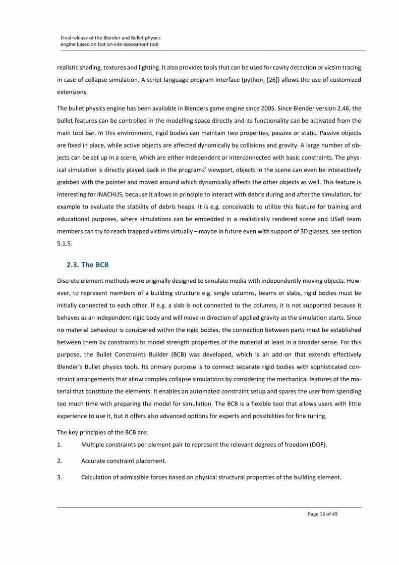
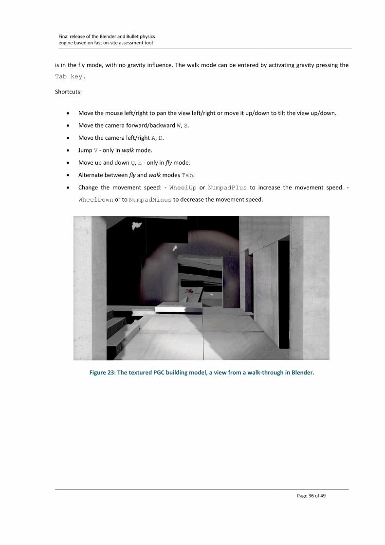
Figure 23: The textured PGC building model, a view from a walk-through in Blender.

Final release of the Blender and Bullet physics engine based on fast on-site assessment tool
Page 37 of 49
Figure 24: The shortcuts for steering during fly/walk mode.
5.1.3. Dissect model
The 3D model can be intuitively cut to unveil the inner structure of a debris heap, see Figure 25. This functionality
in Blender is particularly interesting to quickly assess if there are any hollow spaces big enough for victims to
survive. This method gives a first quick overview of possible voids before the model is further examined by the
Cavity Identification Tool, a stand-alone development of WP3 in INACHUS.
To slice the model:
Hotkey: Alt-B
A selection area is drawn with: left mouse button
The parts of the model that are not in the selection area, are masked out. To restore the model to its entity Alt-
B is pressed again. This technique works even while the animation with the collapse sequence is played back.
Figure 25: Slicing through the model.

Final release of the Blender and Bullet physics engine based on fast on-site assessment tool
Page 38 of 49
5.1.4. Ray-traced rendering
Figure 26: Ray-traced rendering from a simulation frame.
Blender has a variety of tools that help bring realism to still renderings of 3D models. The tools include a versatile
node based material editor, advanced texture mapping and cycles which is a raytracing based render engine.
With enough of processing power, that nowadays is provided by the graphics processing unit (GPU), even com-
plete collapse sequences can be played back in realistic quality on the fly and in real time. A high degree of
realism can help USaR personnel to get a sense of scale and a better and faster interpretation of the virtual 3D
model, see e.g. Figure 26
5.1.5. Virtual Reality (VR)
The ultimate technology to assess 3D models comes with Virtual Reality (VR) software and equipment. VR offers
an immersive experience to the user by interpreting his body movements and simulating its physical presence in
the virtual environment. Special headsets, for example the HTC Vive, and handheld controllers allow users to
interact with objects in the scene (see e.g. Figure 27). USaR personnel could use this technology for true-to life
experiences. Currently, proper VR experience is not possible from within Blender. The collapse model needs to
be exported from Blender into a game engine such as Unreal or Unity, which are both optimized for real-time 3D
playback. However, there are developments on the way to have real-time stereoscopic rendering for VR inte-
grated straight in Blender (Blender VR [29]).

Final release of the Blender and Bullet physics engine based on fast on-site assessment tool
Page 39 of 49
Figure 27: Collapse model evaluated with VR equipment by Futurice.
5.2. Collapse assessment with Blender
A collapse simulation aims in the first place to represent the likely damage pattern and/or debris formation, but
it can be further exploited to investigate the consequences of a building collapse in more detail.
5.2.1. Victim tracing
The amount and location of individuals before a collapse is a very helpful information that can help track the
location of victims throughout the course of the collapse. This information can help USaR teams to allocate their
rescue efforts more efficiently. Beside its powerful visualisation tools, Blender has a rich inbuilt functionality that
is not directly linked with the BCB but can be used to investigate the further reaching consequences of a building
collapse. Blenders Particle System allows the placement of dummies based on location maps2. A location map
shows in grey scale gradients the probable location of occupants. For example, an auditorium or a restaurant
might be indicated in light grey, technical spaces and service rooms in dark grey, Figure 27. In Blender those maps
are applied to the building model floor by floor and the particle system distributes dummies, simplified repre-
sentations of humans, based on the intensity of the grey scale. The dummies are interacting physically with the
collapse simulation and are affected by gravity. A rough estimation where individuals might be after the collapse
can be achieved, Figure 28. Better results in terms of victim localization can be achieved if secondary structures
like glass or bannisters (that usually are not represented in the model) are considered due to the fact that such
structures form in reality additional barriers.
2 This map has to be built currently by the user. It is conceivable that such maps would be made available for each floor of a building to be simulated.

Final release of the Blender and Bullet physics engine based on fast on-site assessment tool
Page 40 of 49
Figure 28: Occupancy map of a hypothetical public event at the PGC, person/Net Internal Area.
Figure 29: Traced dummies during the PGC building simulation.
5.2.2. Visualization of relative displacements
The here presented DEM implementation cannot visualize the magnitude of internal forces. The reason for this
lies in Blender’s Python API, which enables add-ons like the BCB to connect directly to internal Blender data and
functions, but until today provides no possibility to directly access the forces that the Bullet engine evaluates
during simulations. However, displacements of neighbouring rigid bodies, which are caused by these forces, can
be visualized and give indications where zones of high strains are located. In Figure 30 rigid bodies with a high
relative displacement with regard to its adjacent body are coloured red, bodies with low relative displacements
are marked blue.

Final release of the Blender and Bullet physics engine based on fast on-site assessment tool
Page 41 of 49
Figure 30: Visualization of the relative displacement of the shear core of the PGC building after its failure.
5.2.3. Cavity identification
It is of paramount interest to obtain hints where cavities have formed in which victims might be trapped. Rescue
paths can then be planned that lead to their evacuation. By using Blenders Modifier Stack, possible cavity loca-
tions can be highlighted. Modifiers in Blender are automatic operations that affect the shape of an object in a
revocable way. To detect cavities in a debris, several modifiers are combined. In a first step, an array modifier
encloses the whole model with planes that are stacked on top of each other with a pre-set distance. A vertex
weight proximity modifier is then used to detect the relative distances on those planes to the debris mesh (Target
Object) and creates a weight paint map for each plane. A mask modifier then blanks out the parts of the planes
that lay within the debris mesh. Finally, a solidify modifier extrudes the planes to fill the gaps between the planes.
The result is an approximated three- dimensional representation of the voids, see Figure 31.
Figure 31: Representation of voids by applying Blenders modifier system.

Final release of the Blender and Bullet physics engine based on fast on-site assessment tool
Page 42 of 49
6. Summary and Conclusion The here presented simulation approach builds and relies on the Bullet physics engine, whose algorithms are
designed to serve interactive gaming applications and their needs for visual appealing physics simulations that
run in real time. Underlying algorithms derive from DEM and its speed optimized RBD adaptation. The authentic
simulation of structural mechanical problems is in general not a concern for the developers of interactive physics
engines. The special challenge for LUAS was to adapt the method to the scopes of the INACHUS research and to
extend the accuracy by maintaining its speed.
To replicate the bonding and the physical interaction of structural elements in a more plausible way than it is
currently done in real time gaming applications, the Bullet Constraint Builder (BCB) was developed. This set of
scripts attempts to set up – as realistically as possible – a multitude of constraining parameters to describe all
relevant degrees of freedom, providing to the simulation tool the functionalities to replicate the structural be-
havior. Elements are connected with sophisticated constraint arrangements that are monitored during the sim-
ulation for exceedance of admissible material strength values. Additional springs allow the consideration of duc-
tility. The additional constraints naturally slows down the simulation speed and shifts it further away from real-
time, which is aggravated by the current deficient object management in Blender.
Two issues that were broadly discussed with the other WP3 partners during the development of this DEM
method was its slow speed performance and the level of accuracy that could be expected from it.
The simulation speed was improved in two ways: Firstly, the overall time for the preparation of a simulation
model was largely reduced by adding pre-processing tools to the BCB that automatize much of the process. Sec-
ondly, by utilizing a special blender version, the Fracture Modifier, that incorporates a better object management
approach. Running the simulations through the FM boosts the simulation speed considerably. It is expected that
Blender will incorporate advanced object storage capabilities in the upcoming official release 2.80 and that the
simulation speed will drastically improve with the official Blender version as well.
The concern of the simulation accuracy could not definitely be mitigated. Even though averaged engineering
formulas are the bases for the force evaluations, tests on component level (7.1) have shown that a rather large
scattering of load bearing capabilities of identical load bearing elements can occur under certain circumstances.
The reason for this behaviour could not be determined with certainty, but it is suspected that it is due to the way
the Bullet engine prioritizes force evaluations in cases where rigid bodies with big dimensional differences are
connected.
The study of the Pyne Gould building in Christchurch, NZ, documented in [1], showed that similar debris pattern
as observed in reality can be achieved with this DEM method.
Finally, specific examples of unique visualisation features of the results in Blender, maybe with support of Virtual
Reality in future, makes the approach – especially with regard to training purposes for USaR teams – unique.

Final release of the Blender and Bullet physics engine based on fast on-site assessment tool
Page 43 of 49
7. APPENDIX In this appendix, some relevant findings and additional information are collected that will give more insight to
the interested reader.
7.1. High scatter of load bearing capacity of identical beams
Tests on component level (YU beam experiment, [1]) have shown that the load bearing capacity of identical
beams in an array scatters considerably, Figure 33.
Figure 32: Arrangement of ten identical beams break under different applied load.
Figure 33: Scattering of load bearing capacity in beam arrays.
Tests indicate that the observed high scatter stems from big differences in the lengths of rigid bodies that com-
pose a structural element and not from low discretization levels per se. If an element is composed of rigid bodies

Final release of the Blender and Bullet physics engine based on fast on-site assessment tool
Page 44 of 49
with similar length high scatter of the load carrying capacity can be avoided, see Figure 34, Figure 35. Further
clarification is required regarding the reasons for this inconsistent behaviour.
Figure 34 Principle of discretization in equal length.
Figure 35: Scattering of load bearing capacity is eliminated when the beam is composed of rigid bodies with equal length.
7.2. Influence of time steps
The influence of time steps on the simulation can be well illustrated with the second test on component level
(PENG experiment, [1]). This test has shown that the actual deformation of the structure is highly dependent on
the chosen timestep. Figure 36 exhibits observable differences in the deformation for a different number of steps
per second, while the bearable load before collapse does not change and remains stable.
1000 steps/sec

Final release of the Blender and Bullet physics engine based on fast on-site assessment tool
Page 45 of 49
Figure 36: Differences in the deformation depending on chosen time steps.
7.3. Correcting factor
Test series disclosed certain variations for the necessary correcting factor for the evaluation of the moments
threshold in Blender that varied with the length of the cantilevers. An average correcting factor of 1.5 seems
adequate, see Figure 48.
Figure 37: Test series to evaluate the correcting factor for the momenta thresholds.
7.4. Simulation of a brick building
Three of the four building chosen from the Vitruv building library had the main supporting structure in reinforced concrete, one exception is the historic brick building 11 from the Vitruv library [30]. Figure 38 and Figure 39 show the explosion event and the collapse pattern of building 11 and
Table 3 shows the strength values for the materials that were used in the BCB.

Final release of the Blender and Bullet physics engine based on fast on-site assessment tool
Page 46 of 49
Figure 38: Building 11- explosion scenario S2, orthographic rear view.
5 sec after explosion, orthographic front view After collapse, from top
After collapse, perspective After collapse, from side
Figure 39: Building 11- Explosion S2 mode of collapse.

Final release of the Blender and Bullet physics engine based on fast on-site assessment tool
Page 47 of 49
Table 3: Strength values used for the materials of the Vitruv building 11.
7.5. Compressive arch and catenary action
The YU beam experiment [1] drew attention to two complex structural mechanisms that increase the load bear-
ing capacity of a component even after failure initiation. While a DEM simulation may indicate a complete struc-
tural failure after generic and spring constraints have failed, – in reality so called compressive arch and catenary
actions help to build up additional resistance and prevent the structure from total collapse at this point. Addi-
tional strength reserves are mobilized by a complex equilibrium of internal forces that cannot be traced with this
approach, this inability calls for a critical interpretation of the DEM simulation results.
7.6. Video links
BCB presentation at the Blender conference 2015 https://www.youtube.com/watch?v=Razr6RJ5-B4
Collapse simulation of the PGC building in Christ-church, 2011
https://inachuslaurea.word-press.com/2016/06/14/simulation-of-the-earth-quake-in-christchurch-2011/
Blender educational tool for first responders https://www.youtube.com/watch?time_con-tinue=210&v=9RN3IhAZSHc
Simulation of an extraordinary building collapse in Chennai, Moulivakkam, India
https://inachuslaurea.word-press.com/2016/08/31/simulation-of-a-tragedy-in-chennai-india/
Urban Search and Rescue virtual training tool proto-type
https://inachuslaurea.word-press.com/2016/10/30/urban-search-and-rescue-virtual-training-tool-prototype/
Simulation of Vitruv building no 2 https://www.youtube.com/watch?time_con-tinue=6&v=S9jVOkjgsjw
Simulation of Vitruv building no 3 https://www.youtube.com/watch?v=3875PaosMJ0
Simulation of Vitruv building no 9 https://www.youtube.com/watch?v=MYEEzcjTR3w
Simulation of Vitruv building no 11 https://www.youtube.com/watch?v=CIu_xVdlHt4
Simulation of the 2nd pilot case, the demolition of the Sanofy building in Lyon
https://www.youtube.com/watch?time_con-tinue=2&v=pBBkz-yEHsc

Final release of the Blender and Bullet physics engine based on fast on-site assessment tool
Page 48 of 49
8. REFERENCES
[1] Riedel. W., Grunwald C., Inachus Deliverable 3.2: Report on Model Enhancement and Validation Cases,” Freiburg, 2016.
[2] Cundall, P.A., “A Computer Model for Simulating Progressive, Large-Scale Movements in Blocky Rock Systems,” Paper II-8. Symposium Soc. "International Mechanique des Roches", no. Cundall, P. A., A Computer Model for Simulating Progressive, Large-Scale Movements in Blocky Rock Systems. Paper II-8. Symposium Soc. "International Mechanique des Roches". Nancy, 1971, Nancy, 1971.
[3] Cundall, P.A., Strack, O.D.L.: A discrete numerical model for granular assemblies, Geotechnique 29 (1), p. 47-65, 1979
[4] Williams, J.R., Hocking, G., Mustoe, G.G.W.: The theoretical basis of the discrete element method, in: Middleton, J. (ed.): Proceedings of NUMETA ’85 Conference, Swansea, pp. 897-906, 1985
[5] Clearly, P.W.: Discrete Element Modeling of Industrial Granular Flow Applications, Task, Quarterly-Scientific Bulletin, Vol. 2, 385-416
[6] Ghaboussi, J., Barbosa, R.: Three-dimensional discrete element method for granular materials. Int. J. Numer. Anal. Meth. Geomech., 14, p. 451–472, 1990
[7] Hustrulid, A.I., Graham, G.W.M.: Engineering analysis of transfer points using discrete element analysis, Geomechanics Research Center, Colorado School of Mines, 1996.
[8] Bender, J., Erleben, K., Trinkle, J., Coumans, E., Interactive Simulation of Rigid Body Dynamics in Computer Graphics, Computer Graphics forum, 33 (1), 2014
[9] Chen, P.: Quantitative Study of Granular Flow, Mixing and Segregation Using the Discrete Element Method (DEM), Northwestern University Evanstión Illinois 2008
[10] Mirinavičius, A., Markauskas, D., Kačianauskas, R.: Computational Performance of Contact Search During DEM Simulation of Hopper Filling, 10th International Conference of Modern Buildings Materials, Structures and Techniques, Vlinius, Lithuania, May 2010
[11] Schäfer, J., Dippel, S., Wolf, D.E.: Force Schemes in Simulations of Granular Materials, Journal de Physique I, EDP Sciences, 1996, 6 (1), pp.5-20
[12] Walton, O.R., Numerical Simulation of Inelastic, Frictional Particle-Particle Interactions, in: Roco, M.C. (ed.), Particulate Two-Phase Flow, Butterworth-Heinemann, London, 1993, Ch. 25, pp. 884-911
[13] Baraff, D.: An Introduction to Physically Based Modeling: Rigid Body Simulation II-Nonpenetration Constraints, SIGGRAPH Course Notes, 1997, Robotics Institute, Carnegie Mellon University
[14] Williams, J.R., O’Connor, R.: Discrete Element Simulation and the Contact Problem, Arch Computational Methods Eng, 1999, Vol 6 (4), pp. 279-304
[15] Erleben, K.: Stable, Robust, and Versatile Multibody Dynamics Animation, Ph.D.-Thesis, University of Copenhagen, 2005
[16] Bakeer, T.: Collapse Analysis of Masonry Structures under Earthquake Actions, Bauforschung und Baupraxis, Jäger, W., Vassilev, T. (eds), Technische Universität Dresden, 2009
[17] E. Couman, “GitHub,” 2017. [Online]. Available: https://github.com/bulletphysics/bullet3. [Accessed 01 08 2017].
[18] T. B. institute, “Blender,” [Online]. Available: https://www.blender.org/download/. [Accessed 15. 09. 2017].
[19] LUAS, “GitHub,” 2017. [Online]. Available: https://github.com/KaiKostack/bullet-constraints-builder. [Accessed 01 09 2017].

Final release of the Blender and Bullet physics engine based on fast on-site assessment tool
Page 49 of 49
[20] R. Smith, “Open Dynamics engine,” [Online]. Available: http://www.ode.org/. [Accessed 01 08 2017].
[21] Wikipedia, “PhysX,” [Online]. Available: https://en.wikipedia.org/wiki/PhysX. [Accessed 01 08 2017].
[22] T. A. P. Ltd, “True Axis,” [Online]. Available: https://trueaxis.com/. [Accessed 1 8 2017].
[23] Hummel, J., Wolff, R., Stein, T., Gerndt, A., Kuhlen, T.: An Evaluation of Open Source Physics Engines for Use in Virtual Reality Assembly Simulations, in: G. Bebis et. al. (Eds.), ISVC 2012, Part II, LNCS 7432, pp. 346-357, 2012, Springer-Verlag, Berlin Heidelberg
[24] NASA, “Tensegrety Robotics,” [Online]. Available: http://ti.arc.nasa.gov/tech/asr/intelligent-robotics/tensegrity/ntrt/. [Accessed 24.07.2017].
[25] BBZ, “Xron Robotic Surgery Training Software,” [Online]. Available: http://www.bbzsrl.com/xron.html. [Accessed 24.07.2017].
[26] Python, “Python,” [Online]. Available: https://www.python.org/doc/. [Accessed 24.07.2017].
[27] D. B.-V. E.V., BETON-HANDBUCH. Leitsätze für Bauüberwachung und Bauausführung., Wiesbaden: Deutscher Beton-Verein e.V., 1972.
[28] Blender, “Dependency Graph,” Blender, [Online]. Available: https://wiki.blender.org/index.php/Dev:Source/Data_System/Dependency_Graph/Overview. [Accessed 25.07.2017].
[29] Felinto, D., Touraine D. et. al., “BlenderVR,” LIMSI, Laboratoire d'Informatique pour la Mécanique et les Sciences de l'Ingénieur), [Online]. Available: https://blendervr.limsi.fr/doku.php.[Accessed 25.07.2017]
[30] Khalil A., Pellecchia C. , Ricciardi E.M., De Iuliis E., Inachus Deliverable 3.3: “Results report building database and derivation of real-time running AEM models”, 2017
[31] Hoffman J.: Numerical Methods for Engineers and Scientists, Decker AG, New York, Basel 2001
[32] Watt M., Coumans E.:Multithreading for Visual Effects, A K Peters/CRC Press, Boca Raton 2015