Michigan Department of Corrections Institutional and Community Corrections.
•• ,. •••
:·
:·· • • • • • • • • •
•
• •
• •
AN INTEGRATED OVERVIEW
OF THE
FINAL PROJECT REPORTS
GREENHOUSE AND FIELD EVALUATIONS OF LIMESTONE AND GYPSUM FOR REDUCING PHOSPHORUS LEACIDNG AND RUNOFF FROM BEEF CATTLE PASTURES
South Florida Water Management District Contract No. C-10201
Prepared by
University of Florida Institute of Food and Agricultural Services
Range Cattle Research and Education Center Ona, Florida 33865
· Submitted by
J. E. Rechcigl, I. S. Alcordo, L. Boruvka Range Cattle Research and Education Center
A. B. Bottcher Soil and Water Engineering and Technology, Inc .
R. C. Littell Department of Statistics, U.F., IFAS, Gainesville, FL 32611
October 15, 2002

, ..
•
-•
•
•
•
-•
•
•
-•
-•
•
10/17/2002 14:37 9417517639 GCREC BRAD
OCT i'i' 'laG 82157PM UNIV FLORIDA AG 'RE:S CTR ONA .
lilstitute of Food and Agricultural Sc:icDces Range Cattle Res~ and Education Center
October 17, 2002
Ms. Steff:;ny Gornak Senior Environmental Analyst & Project Suvervisor South Florida Water Management District Okeechobee, Fl 34973
Dear Ms_ Gamak:
RECElVED
OCT 2 1 2002 OKEECHOBEE
SERVICE CENTER
PAGE ' 01/01
P P.,· .'q,'~t.:zj .2/2 <.J I
JackE. Reeh~Ph.D. Professor, Soil and Wati!T Sciences 3401 Experiment Station Ona FL 33865-9706 Phone: (803) 735-1314 FAX: (863) 735-1930 E-mail: [email protected]
We are pleased to submit the corrected "An Integrated Overview of the Final Project Reports'' under SFWMD Contract No. C-10201 and our comments to your and the SF\VMD staf£5 ~(1-VM \
Dr. Alcordo had attempted to effect a better integration between the greenhouse results and the field experim=r..:s, hopefully. tD your satisfaction ..
Should yo·l still see some needs to correct certain statements, do not hesitate to call me or Drs. Alcordo 8rtdlor Bottcher.
9:?!# Jack E. R::clicigl Principal Io.vestigator & Director, Gulf Coast Research and Education Center

•
•
--•
•
--•
•
--•
•
•
Responses to the SFWMD Staff Comments on Contract C-10201 Final Report dated August 13, 2002.
• Individual study conclusions and recommendations are given in the Project Summary, Conclusions and Recommendations as suggested. The yield data in the two greenhouse studies and the field experiment are consistent; in all studies there was no response to P fertilization in terms of forage yield. With regards to Ca amendments, the results are also consistent between GS 1 and the field experiment. The field experiment showed slightly elevated P levels in runoff with gypsum and slightly reduced P levels with Ca carbonate. In terms of leachate P concentrations, GS 1 showed very strongly increased P levels with gypsum and reduced P levels with lime, whether calcium carbonate or dolomite. We already made the strongest recommendation for IF AS to reconsider its P recommendation for stargrass and similar improved gras species. The greenhouse and the field experiments
. indicated that regrowth forage containing 0.19 % P or possibly down to 16 % would not benefit from P fertlization.
• We understand that corrections were already made by Dr. Adjie. • See attached CD containing the requested data. • Editorial corrections were made as suggested . • All greenhouse studies used SI units except for conductivity (umho/cm instead ofmS/m) and
% (instead of g/1 OOg) for better comprehension by non-technical people. All fertilizer elements are now consistently expressed as elements as usual and all rates are in kglha. Dr . Bottcher, who prepared his own report, used ft instead ofm or em, °F instead of °C probably because of the his program.
• Re: Rainfall. See p.xxiv, par. 4. • The lime amendment is not mobile and it would be very unlikely that the lime particles were
washed off the plots; gypsum is highly soluble and it could be washed off the plots but gypsum is not a P immobilizer.
• Table GS1-4 cannot be reformatted without reformatting the rest of the tables which could not also be done because of the complexity of the headings.
• Overall means in tables cited were analyzed for overall comparison between horizons P(H) and the letters are correct.
• Values for mg P/kg in the case ofO P (Table GS1-12) are the soil P which were deducted from the P-treated values to get the fertilizer P components.
• For GS1 study, there was some pre-treatment leaching so that we will have to run 3 P fractionations to achieve the suggested comparions. But no sample was taken after pretreatment leaching. There was not a single leaching but a series of 8 leachings so we would have to run 8 multiple regression analysis for each of the 15 treatments. The suggestion is simply impractical.
• Individual study recommendations were removed and integrated into the project recommendations. See comments on the first bullet.
• Title changed to "Influence of Soil Horizons .... ", p.39 . • Tables in GS2 studies were analyzed by Lubos using Duncan, so LSDs are not appropriate. • Chemical speciation modeling may be done for publication in the future. It will not, however
explain the constant amounts of P leached from the Bh, thus, the suggested theory of intrinsic chemical equilibrium between precipitated P and adsorbed P and between adsorbed P and

,..
·• ·-
--!·"'··:'
•
• ····::!'
•
----•
-•
-•
•
--•
• • • • • • •
mobile or leachable P. pp 55. This would be another speculation . p 60. Recommendation was revised and moved to project recommendations as suggested . R2 values, although small or negligible at least give us some measure of the relations, hence are meaningful. Multiple regression may be done in the future for publication. Sentence in former p. 76 has been removed . Grinding was done by Lubos without clearing it with Dr. Rechcigl or Alcordo . Monthly values are now given as suggested . Berm breach is now discussed on p 137, par.3 .

• ~ SOIL & WATER ENGINEERING TECHNOLOGi: INC. ,.
: .. •
•
-----•
-•
•
•
-•
•
November 21, 2002
Ms. Steffany Gornak South Florida Water Management District Okeechobee Service Center 205 North Parrott Ave, Suite 201 Okeechobee, FL 34972
RE: EAAMOD Flow Prediction
Dear Steffany:
RECEIVED
NOV 2 5 2002 OKccCHos·: . ..:.
SERVICE CENTER
As we discussed, the estimates of flow off the fields were made by using EAAMOD. This was done because the paddlewheel samplers flow estimates were quite variable between the plots during storm events. The variability was caused by partial clogging of samplers and the gradient across the plots that caused the northern plots to have greater flow than the southern plots. The paddle wheel data were, however very useful in verifying the EAAMOD predictions as to the occurrence and relative magnitudes between events.
The flow estimates within EAAMOD are determined by the calculation of a continuous water balance which accurately tracks the position of the watertable. When the watertable reaches the surface runoff is initiated. The watertable predictions by EAAMOD were very good as verified by comparison to the measured watertable at the site. The accuracy of the watertable predictions provided a high confidence level in the use ofEAAMOD for providing the flow at the site .
If you have any questions, just let me know.
Sin~ere.l . --_-----------···· ··---...,.
·//~' , -_c/( ~cc~
/
Del Bottcher, Ph.D., P.E.
CC: Jack Rechcigl
3448 N. W 12th Avenue • Gainesville. Florida 32605 • (352) 378-7372 • FAX (352) 378-7472

• i ,. -:• ••
•
•
•
•
-•
•
-•
•
--•
Table of Contents
LIST OF TABLES ........................................................ ix
LIST OF FIGURES ...................................................... xxi
PROJECT EXECUTIVE SUMMARY . . . . . . . . . . . . . . . . . . . . . . . . . . . . . . . . . . . . . xxii
PROJECT INTRODUCTION ............................................... 1
PROJECT OBJECTIVES .................................................. 4
PROJECT MATERIALS AND METHODS . . . . . . . . . . . . . . . . . . . . . . . . . . . . . . . . . . 4
Greenhouse Study 1 (GS1): Individual Soil Horizons with No Stargrass Planted ................................................................ 4
Objectives, treatments, and experimental design ............................... 4 Soil potting, pre-treatment, and treatment application ........................... 5 Sequential leaching ...................................................... 6 Soil sampling and sample preparation ....................................... 6
Greenhouse Study 2, Part I (GS2-I): Individual Soil Horizons Planted to Stargrass ............................................................. 7
Objectives, treatments, and experimental design .............................. ·~ 7 Soil potting, planting of stargrass, and treatment application ..................... 7 Watering and leachate sampling ............................................ 8 Forage sampling and sample preparation ..................................... 8 Soil sampling and sample preparation ....................................... 8
Greenhouse Study 2, Part II (GS2-II): Reconstructed Soil Profile Planted to Stargrass ............................................................. 9
Objectives, treatments, and experimental design ............................... 9 Soil potting, planting of stargrass, and treatment application ..................... 9 Watering and soil water sampling ......................................... 10 Forage sampling and sample preparation .................................... 10 Soil sampling and sample preparation ...................................... 1 0
Field Study 1, Agronomic (AGFS): Phosphorus Fertilization and Effects of Calcium Amendments on Stargrass Forage Yield and Quality and on Soil ................................................................ 11
11

.. :~ . . ,
:1111
•
•
•
•
----•
•
-•
-•
-
Objectives, treatments, and experimental design ................ · .............. 11 Application of treatments . . . . . . . . . . . . . . . . . . . . . . . . . . . . . . . . . . . . . . . . . . . . . . . . 11 Forage sampling and sample preparation .................................... 11 Soil sampling and sample preparation ...................................... 13
Field Study 2, Water Quality (WQFS): Phosphorus Fertilization and Calcium Amendments, Phosphorus in Runoff and Ground Water, Weather Data Collection, and Use of Everglades Agricultural Area Model (EAAMOD) ...................................................... 13
EAAMOD description .................................................. 13 Weather data collection ................................................. 14 Runoffwater sampling .................................................. 15 Ground water sampling . . . . . . . . . . . . . . . . . . . . . . . . . . . . . . . . . . . . . . . . . . . . . . . . . . 15
Leachates and Soil Water Preparation and Chemical Analyses ................... 15
Phosphorus quality assurance/quality control (QNQC) ........................ 15 Greenhouse studies ..................................................... 16 Field studies .......................................................... 16
Stargrass Forage Analyses ................................................. 16
Soil Analyses . . . . . . . . . . . . . . . . . . . . . . . . . . . . . . . . . . . . . . . . . . . . . . . . . . . . . . . . . . . . . 16
Statistical Analysis ........................................................ 17
PROJECT RESULTS AND DISCUSSION ................................... 18
Greenhouse Study 1 (GSl): Individual Soil Horizons with No Stargrass Planted ............................................................... 18
Flow Volumes and Number of Hours for Matrix Flow ........................ 18
Calcium Amendments and Associated Key Leachate Properties ................ 19 Leachate Ca concentration . . . . . . . . . . . . . . . . . . . . . . . . . . . . . . . . . . . . . . . . . . . . . . . 19 Leachate EC .......................................................... 19 Leachate pH .......................................................... 19
Calcium Amendments and P Concentrations in Leachates ..................... 23 Ap leachates .......................................................... 23 E leachates ........................................................... 25 Bh leachates .......................................................... 25
111

-Phosphorus Mobility and Associated Leachate Properties and Elements ......... 26 -Calcium Amendments and P Losses from Ap, E, and Bh Horizons .............. 26
Effects of Ca Amendments at Three Fertilizer P rates on Soil Properties -and Elements ......................................................... 31 Ap horizon ........................................................... 31 • E horizon ............................................................. 31 Bh horizon ........................................................... 31 -Soil Phosphorus Fractionation ............................................ 35 Ap horizon ............................................................ . E horizon ............................................................. 3 5 .. Bh horizon ........................................................... 35
Greenhouse Study 2, Part I (GS2-I): Individual Soil Horizons Planted -to Stargrass ............................................................ 39
Effects of Soil Horizons on Leachate Properties and Elements .................. 39 -Leachate pH ................................................ : ........... 39 Leachate EC ............................................................ 39 -Calcium ............... · ................................................ 39 Magnesium ............................................................ 39 Potassium .............................................................. 44 • Aluminum ............................................................. 44 Iron ................................................................... 44 Nitrate ................................................................ 44 • Sulfate ................................................................ 44 Chloride ............................................................... 50
• Phosphorus in Leachates ................................................... 50
Relations Between Phosphorus and Leachate Properties and Elements .......... 50 • Leachate pH and P ....................................................... 50 Leachate EC and P ....................................................... 50 Leachate cations and P .................................................... 50 -Leachate anions and P .................................................... 53
• Forage Yield, Phosphorus, and Other Nutrients in Forage ..................... 53 Forage yield and percent dry matter ......................................... 53 Phosphorus and other nutrients in forage ..................................... 54 • Phosphorus and Other Nutrients in Soil .................................... 54 Soil column ............ , ............................................... 54 •
IV •
•

Sod soil ............................................................... 56
Accounting for Soil and Fertilizer Phosphorus ............................... 57
Greenhouse Study 2, Part II (GS2-II): Reconstructed Soil Profile Planted to Stargrass ............................................................ 59
• Calcium Amendments and Associated Leachate Properties .................... 59 Leachate Ca concentration ................................................. 59
·- Leachate EC ............................................................ 59 Leachate pH ............................................................ 59
Calcium Amendments and P Concentrations in Leachates ..................... 67 Phosphorus concentrations in leachates ....................................... 67
- Phosphorus Concentrations and Leachate Properties and Elements ............. 67 Leachate pH and P ....................................................... 67 Leachate EC and P ....................................................... 73 - Cations and P in leachates ................................................. 73 Anions and Pin leachates .................................... ; ............ 74
• Phosphorus Fertilizer and Some Leachate Properties ......................... 76 Leachate Ca concentration ................................................. 76 - Leachate EC ............................................................ 76 Leachate pH ............................................................ 78
- Phosphorus Fertilizer and P Concentrations in Leachates ...................... . Phosphorus concentrations in leachates ....................................... 78
• Factors Affecting P in Leachates in P-fertilized Soil .......................... 78 Fertilizer rates and P ........ : ............................................. 78 Leachate EC and P ....................................................... 78 - Leachate pH and P ....................................................... 78 Cations and Pin leachates ................................................. 82 Anions and P in leachates ................................................. 83
• Effects of Ca Amendments on Stargrass Forage Yield and Quality .............. 86 - Forage yield and percent dry matter ......................................... 86 Phosphorus and other macro nutrients in forage ................................ 86 Micro nutrients in forage .................................................. 86
• Effects of Phosphorus Fertilizer on Stargrass Forage Yield and Quality ......... 88 Forage yield and percent dry matter ......................................... 88 - Phosphorus and other macro nutrients in forage ................................ 88
- v
•
-Micro nutrients in forage .............................. ; ................... 88
Effects of Calcium Amendments on Soil .................................... 88 Ap horizon ............................................................. 88 E horizon .............................................................. 88 -Bh horizon ............................................................. 88 -Effects of Phosphorus Fertilizer on Soil .................................... 92 Ap horizon ............................................................. 92 E horizon .............................................................. 93 • Bh horizon ............................................................. 93
Accounting for Soil and Fertilizer Phosphorus in Ca-amended Soil ............ 93 •
Accounting for Soil and Fertilizer Phosphorus in Soil with No Ca Amendments ......................................................... 96
Field Study 1, Agronomic (AGFS): Phosphorus Fertilization and Effects of Calcium Amendments on Stargrass Forage Yield and Quality and on Soil ............................................................... 98
Effects on Forage Yield and Quality . . . . . . . . . . . . . . . . . . . . . . . . . . . . . . . . . . . . . . 98
Forage Yield and Percent Dry Matter (% DM) . . . . . . . . . . . . . . . . . . . . . . . . . . . . 98 Effects of fertilizer P . . . . . . . . . . . . . . . . . . . . . . . . . . . . . . . . . . . . . . . . . . . . . . . . . . . 98 Effects of lime . . . . . . . . . . . . . . . . . . . . . . . . . . . . . . . . . . . . . . . . . . . . . . . . . . . . . . . . 98 Effects of gypsum . . . . . . . . . . . . . . . . . . . . . . . . . . . . . . . . . . . . . . . . . . . . . . . . . . . . . . 98
Crude Protein (CP) and in vitro Organic Matter Digestibility (IVOMD) . . . . . . . 98 Effects of fertilizer P ................................................... 103 Effects oflime ........................................................ 103 Effects of gypsum ..................................................... 1 03
Macro Nutrients P, K, Ca, Mg, and Ca:P Ratio ........................... 103 Effects of fertilizer P ................................................... 103 Effects of lime ........................................................ 110 Effects of gypsum ..................................................... 110
Micro Nutrients Cu, Fe, Mn, and Zn .................................... 113 Effects of fertilizer P ................................................... 113 Effects of lime ........................................................ 113 Effects of gypsum ..................................................... 113
Time Effects on Forage Yield and Quality ................................. 113
Vl
.. •
•
-•
•
•
•
-.. -•
•

•
,._
---•
•
•
•
•
•
•
•
-•
-
Forage Yield and Percent Dry Matter(% DM) ............................ 113
Crude Protein (CP) and in vitro Organic Matter Digestibility (IVOMD) ....... 113
Macro Nutrients P, K, Ca, Mg, and Ca:P Ratio ........................... 119
Micro Nutrients Cu, Fe, Mn, and Zn .................................... 119
Effects on Soil pH, Macro and Micro Nutrients, and Aluminum ............... 119 Effects of fertilizer P ................................................... 123 Effects oflime ........................................................ 123 Effects of gypsum ..................................................... 125
Soil Phosphorus Fractionation ........................................... 127
Field Study 2, Water Quality (WQFS): Phosphorus Fertilization and Calcium Amendments, Phosphorus in Runoff and Ground Water, Weather Data Collection, and Use of Everglades Agricultural Area Model (EAAMOD) ..................................................... 131
Weather Data and Other Observations .................................... 131 Rainfall ............. · ................................................. 132 Solar radiation ......................................................... 132 Watertable ............................................................ 132 Air and soil temperature ................................................. 132
Water Quality Data and. Quality Assurance ................................ 132 Total P ............................................................... 137 EC ................................................................... 137 pH .................................................................. 137
EAAMOD Calibration and Verification ................................... 139
PROJECT CONCLUSIONS AND RECOMMENDATIONS .................... 144
Greenhouse Studies .................................................... 144
Agronomic and Water Quality Field Experiments .......................... 146
REFERENCES .......................................................... 149
ACKNOWLEDGMENT .................................................. 153
APPENDICES A: Water Sample Collection Protocol .......................... 154
Vll
-APPENDICES B: Quality Assurance: Chemical Analytical Procedures .......... 155 -APPENDICES C: Relations Between OP, TP, and ICAP-P ..................... 156
APPENDICES D: Quality Assurance Samples: Duplicates ..................... 157 -•
•
•
-•
•
-•
•
•
-•
•
•
Vlll •
•

( .. •
-••
•
•
--•
•
--•
-•
•
LIST OF TABLES
Greenhouse Study 1 (GSl): Individual Soil Horizons with No Stargrass Planted
Table GS 1-1. Factorial combinations of Prates (0, 50, 100 kg ha-1 equally split and applied 140 days apart) and Ca amendments- 0 Ca, MG, PG, CC, and DL at 800 kg Ca ha-1
- as treatments .............. 5
Table GS 1-2. pH and total chemical analysis of phosphogypsum (PG) and mined gypsum (MG) .......................................... 5
Table GS1-3. Pre-treatment pH and Mehlich I extractable elements and organic matter (OM) in the top 15-cm layer of Ap, E, and Bh horizons of Immokalee fine sand used in the study .................. 6
Table GS 1-4. Leachate volume during sequential leaching of potted soil horizons of a Spodosol using deionized water for Ap, Ap leachates for E, and E leachates for Bh, average of fifteen treatments and eight leaching events over a 220-d period, with no differences between treatments noted within horizon . . . . . . . . . . . . . . . . . . . . . . . . . . . . . . . . . . . . . . . . . 18
Table GS1-5. Calcium in leachates from potted Ap, E, and Bh horizons of a Spodosol, average of eight leaching events over a 220-d period, without or with fertilizer P (kg P ha-1
) orCa amendments MG (mined gypsum), PG (phosphogypsum), CL (calcium carbonate), and DL (dolomite) applied to Ap at 800 kg Ca ha-1
••••••••••••••••• 20
Table GS 1-6. Electrical conductivity (EC) of leachates from potted Ap, E, and Bh horizons of a Spodosol, average of eight leaching events over a 220-d period, without or with fertilizer P (kg P ha-1
) orCa amendments MG (mined gypsum), PG (phosphogypsum), CL (calcium carbonate), and DL (dolomitic limestone) applied to Ap at 800 kg Ca ha-1
•••••••••••••••••••••••••••••••••••••••••••• 21
Table GS 1-7. pH of leachates from potted Ap, E, and Bh horizons of a Spodosol, average of eight leaching events over a 220-d period, without or with fertilizer P (kg P ha-1
) orCa amendments MG (mined gypsum), PG (phosphogypsum), CL (calcium carbonate), and DL (dolomitic limestone) applied to Ap at 800 kg Ca ha-1
•••••••••••••••••••••••• 22
IX

Table GSl-8. Phosphorus in matrix flow from potted Ap, E, and Bh horizons of a Spodosol, average of eight leaching events over a 220-d period, without or with fertilizer P (kg P ha.1
) or Ca amendments MG (mined gypsum), PG (phosphogypsum), CL (calcium carbonate), and DL (dolomite) applied to Ap at 800 kg Ca ha-1
•••••••••••••••••••••••• 24
Table GSl-9. Regression equations for P concentration (Y)t and associated pH, EC, and elements (X)~ in matrix flow through potted Ap, E, and Bh horizons of a Spodosol at all rates of fertilizer P and all Ca amendments; eight sequential leaching events over a 220-d period using 11 em of deionized water each time applied to Ap with the Ap leachate applied to E, and E leachate applied to Bh soil ........... 27
Table GS 1-10. Regression equations for P leached (Y)t from potted Ap horizon of a Spodosol and em of deionized water applied (X)t; influence
---•
•
•
of Ca amendments MG (mined gypsum), PG (phospho gypsum), • CL (calcium carbonate), and DL (dolomite) applied at 800 kg Ca ha-1 at three rates ofP ......................................... 28
Table GS 1-11. Accounting for total+ P leached (retained) from potted Ap horizon of a Florida Spodosol (Immokalee fine sand) fertilized at three rates ofP (0, 50, and 100 kg ha-1
) and amended with Ca-amendments applied at 800 kg Ca ha-1 and from the E and the Bh horizons after 8 leachings, the Ap with 88 em of water, theE with Ap leachates, and the Bh with E leachates, over a period of 220 days .............. 29
Table GS 1-12. Accounting for fertilizer+ P leached (retained) from potted Ap horizon of"a Florida Spodosol (Immokalee fine sand) fertilized at three rates ofP (0, 50, and 100 kg ha-1
) and amended with Ca-amendments applied at SOO kg Ca ha-1 and from the E and Bh horizons after 8 leachings, the Ap with 88 em ofwater, theE with Ap leachates, and the Bh with E leachates, over a period of220 days ................................................ 30
Table GS1-13. pH, EC, organic matter (OM), and Mehlich I extractable elements in potted Ap horizon of a Florida Spodosol (Immokalee fine sand) fertilized at three rates ofP (0, 29.2, and 58.4 mg kg-1) as influenced by Ca amendments (A) applied at 800 kg Ca ha-1 in the form of mined gypsum (MG), phosphogypsum (PG), calcium carbonate (CL), or dolomite (DL) after 8 leachings with 88 em of water over a period of 220 days ......................................... 32
X
•
•
•
•
•
---•
•
•
•

• .. .:·-
••
·• 't..
•
•
•
-•
•
•
•
•
•
--•
Table GS1-140 pH, EC, organic matter (OM), and Mehlich I extractable elements in potted E horizon of a Florida Spodosol (Immokalee fine sand) after 8 leachings over a period of 220 days using Ap leachates from potted Ap horizon fertilized at three rates ofP (0, 2902, and 58.4 mg kg-1) and amended with Ca amendments (A) applied at 800 kg Ca ha-1 in the form of mined gypsum (MG), phosphogypsum (PG), calcium carbonate (CL), or dolomite (DL) and leached with 88 em of water 8 times over the same period days 0 0 0 0 0 0 0 0 0 0 0 0 0 0 0 0 0 0 0 0 0 0 0 33
Table GS1-150 pH, EC, organic matter (OM), and Mehlich I extractable elements in potted Bh horizon of a Florida Spodosol (Immokalee fine sand) after 8 leachings over a period of 220 days using E leachates from potted E horizon previously leached with Ap leachates from potted Ap horizon fertilized at three rates ofP (0, 29.2, and 58.4 mg P kg-1)
and amended with Ca amendments (A) applied at 800 kg Ca ha-1
in the form of mined gypsum (MG), phosphogypsum (PG), calcium carbonate (CL), or dolomite (DL) and leached with 88 em of water 8 times over the same period 0 0 0 0 0 0 0 0 0 0 0 0 0 0 0 0 0 0 0 0 0 0 0 0 0 0 0 0 0 0 0 0 0 0 34
Table GS 1-160 Phosphorus fractions in potted Ap horizon of a Florida Spodosol (Immokalee fine sand) fertilized at three rates ofP {0, 50, and 100 kg ha-1
) and amended with Ca amendments (A) applied at 800 kg ha- 1
in the form of mined gypsum (MG), phosphogypsum (PG), calcium carbonate (CL), or dolomite (DL) after 8 leachings with 88 em of water over a period of 220 days 0 0 0 0 0 0 0 0 0 0 0 0 0 0 0 0 0 0 0 0 0 0 0 0 0 0 0 0 0 0 0 0 36
Table GS 1-17 0 Phosphorus fractions in potted E horizon of a Florida Spodosol .. (Immokalee fine sand) after 8 teachings over a period of 220 days using Ap leachates from potted Ap horizon fertilized at three rates ofP (0, 50, and 100 kg ha-1
) and amended with Ca amendments (A) applied at 800 kg ha-1 in the form of mined gypsum (MG), phosphogypsum (PG), calcium carbonate (CL), or dolomite (DL) and leached 8 times with 88 em of water over the same period 0 0 0 0 0 0 0 0 37
Table GS 1-180 Phosphorus fractions in potted Bh horizon of a Florida Spodosol (Immokalee fine sand) after 8 leachings over a period of 220 days using E leachates from potted E horizon previously leached with Ap leachates from potted Ap horizon fertilized at three rates ofP (0, 50, and 100 ha-1
) and amended with Ca amendments (A) at 800 kg ha- 1 in the form of mined gypsum (MG), phosphogypsum (PG), calcium carbonate (CL), or dolomite (DL) and leached 8 times with 88 em of water over the same period 0 0 0 0 0 0 0 0 0 0 0 0 0 0 0 0 0 0 0 0 0 0 0 0 0 0 0 0 38
XI

Greenhouse Study 2, Part I (GS2-I): Individual Soil Horizons Planted to Stargrass
Table GS2-I-l. Treatments (horizons and pure sand) and P fertilizer (TSP) used ......... 7
Table GS2-I-2. Pre-treatment pH and Mehlich I extractable elements in Immokalee fine sand used in Greenhouse Study 2, Part I and Part II ............... 8
Table GS2-I-3. pH ofleachates from potted horizons oflmmokalee fine sand, a Spodosol, and from pure sand fertilized at 50 kg P ha-1 using fine-ground TSP, unless indicated otherwise, and planted to stargrass .................................................... 40
Table GS2-I-4. Electrical conductivity (EC) ofleachates from potted horizons of Immokalee fine sand, a Spodosol, and from pure sand fertilized at 50 kg P ha-1 using fine-ground TSP, unless indicated otherwise, and planted to· stargrass ........................................ 41
Table GS2-I-5. Ca concentrations in leachates from potted horizons oflmmokalee fine sand, a Spodosol, and from pure sand fertilized at 50 kg P ha-1
using fine-ground TSP, unless indicated otherwise, and planted to stargrass .................................................... 42
Table GS2-I-6. Mg concentrations in leachates from potted horizons oflmmokalee fine sand, a Spodosol, and from pure sand fertilized at 50 kg P ha-1
using fine-ground TSP, unless indicated otherwise, and planted to star grass ............ : ....................................... 4 3
Table GS2-I-7. K concentrations in leachates from potted horizons oflmmokalee fine sand, a Spodosol, and from pure sand fertilized at 50 kg P ha- 1
using fine-ground TSP, unless indicated otherwise, and planted to stargrass .................................................... 45
Table GS2-I-8. Al concentrations in leachates from potted horizons oflmmokalee fine sand, a Spodosol, and from pure sand fertilized at 50 kg P ha- 1
using fine-ground TSP, unless indicated otherwise, and planted to stargrass .................................................... 46
Table GS2-I-9. Fe concentrations in leachates from potted horizons of Immokalee fine sand, a Spodosol, and from pure sand fertilized at 50 kg P ha-1
using fine-ground TSP, unless indicated otherwise, and planted to stargrass .................................................... 4 7
Xll
----•
•
-•
•
•
-•
•
-•
•
-•
•
•
-•
•
• .. •
•
•
•
-•
--•
Table GS2-I-10. Nitrate concentrations in leachates from potted horizons of Immokalee fine sand, a Spodosol, and from pure sand fertilized at 50 kg P ha·1 using fine-ground TSP, unless indicated otherwise, and planted to stargrass ....................................... 48
Table GS2-I-ll. Sulfate concentrations in leachates from potted horizons of Immokalee fine sand, a Spodosol, and from pure sand fertilized at 50 kg P ha·1 using fine-ground TSP, unless indicated otherwise, and planted to stargrass ....................................... 49
Table GS2-I-12. Chloride concentrations in leachates from potted horizons of Immokalee fine sand, a Spodosol, and from pure sand fertilized at 50 kg P ha·1 using fine-ground TSP, unless indicated otherwise, and planted to stargrass ....................................... 51
Table GS2-I-13. Phosphorus concentrations in leachates from potted horizons of Immokalee fine sand, a Spodosol, and from pure sand fertilized at 50 kg P ha·1 using fine-ground TSP, unless indicated otherwise, and planted to stargrass ....................................... 52
Table GS2-I-14. Relationships between P concentrations (Y = mg P/unit X) and pH, EC, cation, and anions (X) in leachates from all potted media (Ap, E, and Bh horizons oflmmokalee fine sand and from pure . sand) planted to stargrass and fertilized twice at 50 kg P ha·1
•••••••••• 53
Table GS2-I-15. Total dry matter (DM) yield, percent dry matter (%DM), and total elemental uptake by stargrass planted in potted Ap, E, and Bh horizons of Immokalee fine sand, a Spodosol, and in pure sand fertilized at 50 kg P ha·1 applied twice using fine-ground TSP, unless indicated otherwise ................................. 55
Table GS2-I-16. Soil pH and certain Mehlich I extractable elements in potted soil horizons of Immokalee fine sand and in pure sand planted to stargrass and fertilized twice at 50 kg P ha·1 with the second P application made 14 weeks after the first ........................ 56
Table GS2-I-17. Accounting for Pin soil horizons oflmmokalee fine sand and in pure sand planted to stargrass and fertilized twice at 50 kg P ha·1
with the second P application made 14 weeks after the first ........... 57
Greenhouse Study 2, Part II (GS2-II): Reconstructed Soil Profile Planted to Stargrass
Table GS2-II-l. Experimental treatments (P applied twice for a total ofO, 25, 50, 100 kg P ha-1
) ••••••••••••••••••••••••••••••••••••••••••••••••• 9
Xlll

Table GS2-II-2. Ca concentrations in shallow wellleachates from reconstructed soil profile of Immokalee fine sand planted to stargrass fertilized at 50 kg P ha·1 and amended with Ca amendments ................... 60
Table GS2-II-3. Ca concentrations in deep wellleachates from reconstructed soil profile of Iminokalee fine sand planted to stargrass fertilized at 50 kg P ha·1 and amended with Ca amendments ..................... 61
Table. GS2-II-4. Ca concentrations in bottom leachates from reconstructed soil profile of Immokalee fine sand planted to stargrass fertilized at 50 kg P ha·1 and amended with Ca amendments .................... 62
Table GS2-II-5. EC of shallow wellleachates from reconstructed soil profile of Immokalee fine sand planted to stargrass fertilized at 50 kg P ha·1 and amended with Ca amendments .......................... 63
Table GS2-II-6. EC of deep wellleachates from reconstructed soil profile of Immokalee fine sand planted to stargrass fertilized at 50 kg P ha·1 and amended with Ca amendments .......................... 64
Table. GS2-II-7.EC ofbottom leachates from reconstructed soil profile of Immokalee fine sand planted to stargrass fertilized at 50 kg P ha·1 and amended with Ca amendments .......................... 65
Table GS2-II-8. pH of shallow wellleachates from reconstructed soil profile of Immokalee fine sand planted to stargrass fertilized at 50 kg P ha·1 and amended with Ca amendments .......................... 66
Table GS2-II-9. pH of deep wellleachates from reconstructed soil profile of Immokalee fine sand planted to stargrass fertilized at 50 kg
...
P ha·1 and amended with Ca amendments .......................... 68
Table GS2-II-lO.pH ofbottom leachates from reconstructed soil profile of Immokalee fine sand planted to stargrass fertilized at 50 kg P ha·1 and amended with Ca amendments ......................... 69
Table GS2-II-ll.Phosphorus concentrations in shallow wellleachates from reconstructed soil profile of Immokalee fine sand planted to stargrass fertilized at 50 kg P ha·1 and amended with Ca amendments ............................................. 70
Table GS2-II-12.Phosphorus concentrations in deep wellleachates from reconstructed soil profile of Immokalee fine sand planted to stargrass fertilized at 50 kg P ha·1 and amended with Ca amendments ................................................ 71
XIV
----•
--•
•
.. -•
•
-----•

•
..
•
•
•
•
•
•
•
• •
-•
•
--
Table. GS2-II-13.Phosphorus concentrations in bottom leachates from reconstructed soil profile of Immokalee fine sand planted to stargrass fertilized at 50 kg P ha·1 and amended with Ca amendments ................................................ 72
Table GS2-II-14. Relationships between leachate P concentrations (Y) and pH (X) of leachates from reconstructed soil profile of Immokalee fine sand planted to stargrass fertilized twice at 50 kg P ha·1 and amended with Ca amendments (all amendments) ....... 73
Table GS2-II-15. Relationships between leachate P concentrations (Y) and EC (X) of leachates from reconstructed soil profile of Immokalee fine sand planted to stargrass fertilized twice at 50 kg P ha·1 and amended with Ca amendments (all amendments) .................. 74
Table GS2-II-16. Relationships between leachate P concentrations (Y) and cations (X) in leachates from reconstructed soil profile of Immokalee fine sand planted to stargrass fertilized twice at 50 kg P ha·1 and amended with Ca amendments (all amendments) ........ 75
Table GS2-II-17. Relationships between leachate P concentrations (Y) and anions (X) in leachates from reconstructed soil profile of Immokalee fine sand planted to stargrass fertilized twice at 50 kg P ha·1 and amended with Ca amendments (all amendments) ....... 76
Table GS2-II-18. Ca concentrations in leachates sampled at three depths from reconstructed soil profile of Immokalee fine sand planted to stargrass fertilized at four rates of P, no Ca amendments . . . . . . . . . . . . 77.
Table GS2-II-19. EC ofleachates sampled at three depths from reconstructed soil profile of IJTI?lokalee fil).e sand planted to stargrass fertilized at four rates of P, no Ca amendments. . ................... 79
Table GS2-II-20. pH ofleachates sampled at three depths from reconstructed soil profile of Immokalee fine sand planted to stargrass fertilized at four rates ofP, no Ca amendments ............................. 80
Table GS2-II-21. Phosphorus concentrations in leachates sampled at three depths from reconstructed soil profile of Immokalee fine sand planted to stargrass fertilized at four rates of P, no Ca amendments. . ......... 81
Table GS2-II-22. Relationships between leachate P concentrations (Y) and EC (X) of leachates from reconstructed soil profile of Immokalee fine sand planted to stargrass fertilized twice at 0, 12.5, 25, and 50 kg P ha·1
,' no Ca amendments ............................... 82
XV

Table GS2-II-23. Relationships between leachate P concentrations (Y) and pH (X) ofleachates from reconstructed soil profile oflmmokalee fine sand planted to stargrass fertilized twice at 0, 12.5, 25, and 50 kg P ha·1
, no Ca amendments. . .............................. 83
Table GS2-II-24. Relationships between leachate P concentrations (Y) and cations (X) in leachates from reconstructed soil profile oflmmokalee fine sand planted to stargrass fertilized twice at 0, 12.5, 25, and 50 kg P ha·1
, no Ca amendments. . .............................. 84
Table GS2-II-25. Relationships between leachate P concentrations (Y) and anions (X) in leachates from reconstructed soil profile oflmmokalee fine sand planted to stargrass fertilized twice at 0, 12.5, 25, and 50 kg P ha· 1
, no Ca amendments. . .............................. 85
Table GS2-II-26. Total dry matter (DM) yield, percent dry matter (%DM), and total elemental uptake by stargrass planted in reconstructed soil profile oflmmokalee fine sand fertilized at 50 kg P ha·1 applied twice and amended with Ca amendments. . ....................... 87
Table GS2-II-27. Total dry matter (DM) yield, percent dry matter (%DM), and total elemental uptake by stargrass planted in reconstructed soil profile of Immokalee fine sand fertilized at four rates of P applied -twice, no Ca amendments ...................................... 89
Table GS2-II-28. Soil pH and Mehlich I extractable elements in Ap horizon of reconstructed soil profile of Immokalee fine planted to stargrass fertilized twice at 50 kg ha·1
, with the second P application applied 14 weeks after the first, and amended with Ca amendments. . ......... 90
Table GS2-II-29. Soil pH and Mehlich I extractable elements in E horizon of reconstructed soil profile of Immokalee fine with the Ap horizon
•
-•
-•
•
•
•
•
•
•
planted to stargrass fertilized twice at 50 kg ha·1, with the second P •
application applied 14 weeks after the first, and amended with Ca amendments ................................................ 91
Table GS2-II-30. Soil pH and Mehlich I extractable elements in Bh horizon of reconstructed soil profile of Immokalee fine with the Ap horizon planted to stargrass fertilized twice at 50 kg ha·1
, with the second P application applied 14 weeks after the first, and amended with Ca amendments. . ............................................... 92
XVI
-•
•
•
-•

..
•
•
-•
-•
-•
•
•
•
---
Table GS2-II-31. Soil pH and Mehlich I extractable elements in Ap horizon of reconstructed soil profile of Immokalee fine planted to stargrass fertilized twice at four rates of P, with the second P application applied 14 weeks after the first, no Ca amendments. . ............... 93
Table GS2-II-32. Soil pH and Mehlich I extractable elements in E horizon of reconstructed soil profile of Immokalee fine with the Ap horizon planted to stargrass fertilized twice at four rates of P, with the second P application applied 14 weeks after the first, no Ca amendments. . .............................................. 94
Table GS2-II-33. Soil pH and Mehlich I extractable elements in Bh horizon of reconstructed soil profile of Immokalee fine with the Ap horizon planted to stargrass fertilized twice at four rates of P, with the second P application applied 14 weeks after the first, no Ca amendments. . .............................................. 94
Table GS2-II-34. Accounting for soil and fertilizer Pin reconstructed soil profile of Irrimokalee fine sand planted to stargrass fertilized twice at 50 kg P ha·1
, with second P application applied 14 weeks after the first, and amended with Ca amendments at 2 Mg ha·1
• • ••••••••••••• 95
Table GS2-II-35. Accounting for soil and fertilizer Pin reconstructed soil profile of Immokalee fme sand planted to stargrass fertilized twice at four rates ofP, with the second P application applied 14 weeks after the first, no Ca amendments. . ............................. 97
Field Study 1, Agronomic (AGFS): Phosphorus Fertilization and Effects of Calcium Amendments on Stargrass Forage Yield and Quality and on Soil
Table AGFS-1. Phosphorus fertilizer and Ca amendment rates based on 100% CaC03 or CaS04.2H20 content; P fertilizers applied annually and Ca amendments applied once at the start of the study. . . . . . . . . . . . . . . . . . . . 11
Table AGFS-2. Pre-treatment pH and Mehlich I extractable elements and organic matter (OM) in the top 15-cm layer of Ap, E, and Bh horizons of Immokalee fine sand used in the study . . . . . . . . . . . . . . . . . . . . . . . . . . . .13
Table AGFS-3. Effects ofP fertilizer, calcium carbonate, and mined gypsum on percent dry matter (%DM) and total forage DM yield of stargrass pasture on Immokalee fine sand fertilized annually with P without or with Ca amendment applied once in 1999; 1999 (7 harvests), 2000 (6 harvests), and 2001 (6 harvests) seasons ........................ 99
xvn

Table AGFS-4. Effects ofP fertilizer applied annually without Ca amendments on percent dry matter (%DM) and total forage DM yield of stargrass pasture on Immokalee fine sand; 1999 (7 harvests), 2000 (6 harvests), and 200 1 ( 6 harvests) seasons. . . . . . . . . . . . . . . . . . . . . . . . . . . . . . . . . . 1 00
Table AGFS-5. Effects of calcium carbonate on percent dry matter (%DM) and total forage DM yield of stargrass pasture on Immokalee fine sand applied once in 1999 to plots fertilized annually at 50 kg P ha·1
,
1999 (7 harvests), 2000 (6 harvests), and 2001 (6 harvests) seasons. . .. 101
Table AGFS-6. Effects of mined gypsum on percent dry matter (%DM) and total forage DM yield of stargrass pasture on Immokalee fine sand applied once in 1999 to plots fertilized annually at 50 kg P ha·1
,
1999 (7 harvests), 2000 ( 6 harvests), and 2001 ( 6 harvests) seasons) . 1 02
Table AGFS-7. Effects of P fertilizer, calcium carbonate, and gypsum on percent crude protein (% CP) and in vitro organic matter digestibility (% IVOMD) of stargrass forage from pasture growing on Immokalee fine sand soil, 1999 (7 harvests), 2000 (6 harvests), and 2001 ( 6 harvests) seasons . . . . . . . . . . . . . . . . . . . . . . . . . . . . . . . . . . . . . . . . 1 04.
Table AGFS-8. Effects ofP fertilizer without the amendments on percent crude protein (%CP) and in vitro matter digestibility(% IVOMD) of stargrass forage growing on Immokalee fine sand, 1999 (7 harvests), 2000 (6 harvests), and 2001 (6 harvests) seasons. . ................ 105
Table AGFS-9. Effects of calcium carbonate at 50 kg P ha·1 on percent crude protein (%CP) and in vitro organic matter digestibility(% IVOMD) of stargrass forage growing on Immokalee fine sand, 1999 (7 harvests), 2000 (6 harvests), and 2001 (6 harvests) seasons .................. 106
Table AGFS-1 0. Effects of mined gypsum at 50 kg P ha· 1 on percent crude protein (%CP) and IVOMD of stargrass forage from pasture growing on Immokalee fine sand, 1999 (7 harvests), 2000 (6 harvests), and 2001 ( 6 harvests) seasons ......................................... 1 07
Table AGFS-11. Effects of P fertilizer, calcium carbonate, and gypsum on macro nutrients in stargrass forage from pasture growing on Immokalee fine sand, 1999 (7 harvests), 2000 (6 harvests), and 2001 (6 harvests)
seasons. . ................................................ 108
Table AGFS-12. Effects ofP fertilizer on macro nutrients in stargrass forage from pasture growing on Immokalee fine sand, 1999 (7 harvests), 2000 (6 h'\fVests), and 2001 (6 harvests) seasons. . ................... 109
XVlll
•
-•
•
•
• .. -•
•
-•
•
-•
•
•
•
•

,. ' ,.
•
•
•
•
-• .. -•
•
•
•
•
-
Table AGFS-13. Effects of calcium carbonate on macro nutrients in stargrass forage from pasture growing on Immokalee fine sand, 1999 (7 harvests), 2000 (6 harvests), and 2001 (6 harvests) seasons ............... Ill
Table AGFS-14. Effects of gypsum on macro nutrients in stargrass forage from pasture growing on Immokalee fine sand, 1999 (7 harvests), 2000 (6 harvests), and 2001 (6 harvests) seasons. . ................... 112
Table AGFS-15. Effects ofP fertilizer, calcium carbonate, and gypsum on micro nutrients in stargrass forage from pasture growing on Immokalee fine sand, 1999 (7 harvests), 2000 ( 6 harvests), and 2001 ( 6 harvests)
seasons. . . . . . . . . . . . . . . . . . . . . . . . . . . . . . . . . . . . . . . . . . . . . . . . . . 114
Table AGFS-16. Effects ofP fertilizer on micro nutrients in stargrass forage from pasture growing on Immokalee fine sand, 1999 (7 harvests), 2000 (6 harvests), and 2001 (6 harvests) seasons. . ................... 115
Table AGFS-17. Effects of calcium carbonate on micro nutrients in stargrass forage from pasture growing on Immokalee fine sand, 1999 (7 harvests), 2000 (6 harvests), and 2001 (6 harvests) seasons ............... 116
Table AGFS-18. Effects of. gypsum on micro nutrients in stargrass forage from pasture growing on Immokalee fine sand, 1999 (7 harvests), 2000 ( 6 harvests), and 2001 ( 6 harvests) seasons . . . . . . . . . . . . . . . . . . . . . 11 7
Table AGFS-19. Percent dry matter (%DM), forage DM yields, crude protein (CP), and in vitro organic matter digestibility (IVOMD) of stargrass (harvests 1- 6) pasture on Immokalee fine sand at various P (kg ha-1
) rates applied annually without or with Ca amendments (Mg ha·) mined gypsum (MG) or calcium carbonate (CC) applied once in 1999 with Crop Year as treatments . . . . . . . . . . . . . . . . . . . . . . . 118
Table AGFS-20. Macro nutrients in stargrass forage (harvests 1-6) from pasture on Immokalee fine sand at various P (kg ha-1
) rates applied annually without or with Ca amendments (Mg ha-1
) mined gypsum (MG) or calcium carbonate (CC) applied once in 1999 with Crop Year as treatments. . . . . . . . . . . . . . . . . . . . . . . . . . . . . . . . . . . . . . . . . . . 120
Table AGFS-21. Micro nutrients in stargrass forage (harvests 1-6) from pasture on Immokalee fine sand at various P (kg ha- 1
) rates applied annually without or with Ca amendments (Mg ha-1
) mined gypsum (MG) or calcium carbonate (CC) applied once in 1999 with Crop Year as treatments. . ............................................... 121
XIX

Table AGFS-22. Three-year mean soil pH and Mehlich I extractable elements in Immokalee fine sand profile as influenced by P fertilization (kg ha-1
) applied annually and soil amendments (A) calcium carbonate (CL) or mined gypsum (MG) in A Mg ha-1applied once in 1999 ............................................... 122
Table AGFS-23. Three-year mean effects ofP fertilizer applied annually on soil pH and Mehlich 1 extractable macro nutrients and AI in Immokalee fine sand profile. . . . . . . . . . . . . . . . . . . . . . . . . . . . . . . . . 124
Table AGFS-24. Three-year mean effects of calcium carbonate applied once in 1999 to plots that received 50 kg P ha-1 applied annually on soil pH and Mehlich 1 extractable macro nutrients and AI in Immokalee fine sand profile ................................. 126
Table AGFS-25. Three-year effects of gypsum applied once in 1999 to plots that received 50 kg P ha-1 applied annually on soil pH and Mehlich I extractable macro nutrients and AI in Immokalee fine sand profile .. 128
Table AGFS-26. Phosphorus fractions in Immokalee fine sand profile as influenced by P fertilization and soil amendments (A) calcium carbonate (CL) or mined gypsum (MG), average of 1999-2000 samplings ...... 130
Field Study 2, Water Quality (WQFS): Phosphorus Fertilization and Calcium Amendments, Phosphorus in Runoff and Ground Water, Weather Data Collection, and Use of Everglades Agricultural Area Model (EAAMOD)
Table WQFS-1. Monthly averages of rainfall, depth ofwatertable, solar radiation, and air and soil temperature at Williamson Ranch, Okeechobee, 1999 to 2002 ............................................... 133
Table WQFS-2. Relationships between pH, EC ( ~mho/cm- 1 ), and total P (~g TP L-1
) and Ca amendments and fertilizer Prates in surface runoff (Paddlewheels) and water samples above the spodic (Shallow wells) and below the spodic (Deep wells) horizon .......... 138
Table WQFS-3. Simulated versus observed TP concentrations for 2001 for fertilizer P treatment ........................................ 139
Table WQFS-4. Simulated versus observed TP concentrations for 2001 for Ca treatments . . . . . . . . . . . . . . . . . . . . . . . . . . . . . . . . . . . . . . . . . . . . . . . . 141
XX
•
•
•
-•
• .. •
•
•
• .. -•
-•
•
--

LIST OF FIGURES
Figure AGFS-1. Plot layout for the field stargrass study ........................... 12
• Figure WQFS-1. Watertable above and below the spodic horizon, Williamson Ranch, Okeechobee, 1999 ................................... 134
Figure WQFS-2. Watertable above and below the spodic horizon, Williamson Ranch, Okeechobee, 2000 ................................... 135 - Figure WQFS-3. Watertable above and below the spodic horizon, Williamson Ranch, Okeechobee, 2001-2002 .............................. 136 - Figure WQFS-4. The EAAMOD simulated versus observed watertable levels above and below spodic horizon, Williamson ranch, Okeechobee .... 140 - Figure WQFS-5. The EAAMOD simulated total P (TP) versus observed TP and ortho-P (0-P) concentrations ................................ 142
Figure WQFS-6. The EAAMOD simulated total P (TP) outflow concentrations for 20 years using 1999 weather data each year .................. 142 -
-•
-•
-•
•
• XXI
-
PROJECT EXECUTIVE SUMMARY
The project consisted of( a) agronomic and (b) water quality field experiments with the following objectives: (1) to evaluate the effectiveness ofCa amendments in improving the retention capacity of soils for fertilizer P applied to stargrass pastures, (2) to reevaluate the current IF AS (Institute of Food and Agricultural Sciences) P fertilizer rate recommendations for improved pasture grasses using stargrass as the test crop, (3) to use the data collected to calibrate the EAAMOD (Everglades Agricultural Area Model) computer model and (4) to use the calibrated computer model to extend the field results to other field conditions and untested forages.
Agronomic Field Study (AGFS). The treatments consisted of 0, 12.5. 25, and 50 kg P ha-1
applied annually (April to May) for three years (1999, 2000, and 2001) to established stargrass (Cynodon sp.) pasture in Okeechobee Co. at the Williamson Cattle Ranch. Soil was Immokalee fine sand (sandy, siliceous, hyperthermic Arenic Alaquods). Calcium amendments were calcium carbonate and mined gypsum applied once at the start of the study (1999) at 0, 2, and 4 Mg ha-1
, pure basis, to plots that received 50 kg P ha-1
• Treatments were replicated four times using 32 plots each measuring 15m x 30m. Forage samples were collected once every 30-35 days for yield and for forage quality analysis. Forage quality measures analyzed were crude protein (CP), in vitro organic matter digestibility (IVOMD), and macro and micro nutrients. Soils were analyzed for Mehlich I extractable nutrients and for the various P fractions.
Water Oualitv Field Study (WOFS). For use in modeling, a fully automated weather station (Campbell Scientific, Inc.) was installed in the middle of the agronomic study areaonApril26, 1999 to record weather data. Wells (PVC pipes) were also set up to monitor depth of water table at the station. Data collected consisted of the following:
Rainfall· Solar radiation Air temperature Soil temperature at 45 em Watertable above the spodic horizon (hardpan) Watertable below the spodic horizon (hardpan)
The station was provided with a cellular phone communications package that allows for remote access for data downloads and station program maintenance. It also had a voice synthesizer and software that allowed it to call the field staff at the Range Cattle Research and Experiment Station (RCREC) to alert them to a rainfall event so that a sampling trip can be scheduled. The station can also call Soil and Water Engineering Technology, Inc. (SWET, Inc.) in Gainesville if a transducer error has occurred. SWET also does a daily download of data to keep track of the station's performance.
A 15-30 em deep perimeter ditch around each agronomic plot was constructed and a flow integrating sampling device to collect runoff sample (paddlewheel-type) was set in place at each plot. The runoff from the plots flows out into the experimental block drainage ditches and into a main
xxn
--•
•
•
--• •
•
•
•
--•
•
•
•
•
••
,. : ".
.. •
•
•
•
•
•
•
-•
-•
•
•
•
drainage ditch. The sampling devices were inspected every time there was a significant rainfall event; total sample volumes were recorded and small volumes of samples were collected and prepared for storage according to a sampling protocol.
Subsurface or ground water samples were collected at two depths from two wells consisting of 5-cm inside diameter PVC pipes installed at the center of each plot set 0.5 m apart. The "shallow" well pipes have their lower ends down to about 0.5 m (at theE horizon) and those of the "deep" well pipes down to about 1.0 m (at or below the Bh horizon) from the surface of the soil. Water samples were collected at least once each month or after every major rainfall event and prepared for storage according to the sampling protocol. Watertable levels were also measured and recorded every collection time.
Water samples were analyzed for P (ortho-P and total P) using a colorimetric method at a detection limit of 5 ppb, and also by inductively coupled argon plasma (ICAP) spectroscopy at a detection limit of 0.1 ppm. Specific conductivity and pH were also determined .
To help explain and/or confirm field results, three greenhouses studies were conducted during the first year (1999) using similar field treatments at the RCREC. Greenhouse study 1 (GSI) used potted individual soil horizons of Immokalee fine sand, with no stargrass planted, and leached over a 220-day period eight times sequentially, the Ap horizon using deionized water, theE horizon using Ap leachates, and the Bh horizon using E leachates. Greenhouse study 2, part I (GS2-I) also used potted individual soil horizons and pure sand planted to stargrass to determine the influence of individual horizons to fertilizer P applied twice at 50 kg P ha·1 each time imd to determine the capacity ofstargrass to utilize fertilizer P. And greenhouse study 2, part 2 (GS2-II), the greenhouse duplicate of the field experiment, used recon~tructed soil profile oflmmokalee fine sand planted to stargrass and the complete field treatments. Studies GS2-I and GS2-II were watered regularly, and water samples were collected ten times over a 24-week period .
Field and Greenhouse Agronomic Results. The field study showed that P fertilizer did not increase forage yields nor improve forage quality measures such as crude protein (CP) contents and · in vitro organic matter digestibility (IVOMD). Forage from plots where no fertilizer P was applied for three crop years did not show any deterioration in forage yield and in quality on the third year; forage yields were influenced more by crop year, which had distinctly different rainfall levels during the growing season, than by P fertilization. Rainfall, though not an experimental variable, was recorded year-round during the three-year period of the study. Forage yields in greenhouse studies GS2-I and GS2-II also failed to increase with increasing amounts ofP indicating that Immokalee fine sand has sufficient soil P to meet the needs of stargrass for maximum yield.
Greenhouse study GS2-II and the field study showed that P fertilization increased P contents significantly and linearly with P rates. With no differences in forage yields within each study, P contents in regrowth forage ranged from 0.27 to 0.29 for GS2-I, 0.22 to 0.30 for GS2-II, and 0.19 to 0.34% for the field study. These data would indicate that stargrass pastures on Immokalee fine sand with regrowth forage containing 0.19 % P do not need any P fertilizer for maximum yield. Evaluation ofP uptake by stargrass indicated that P fertilization only helped to build up soil P at the
xxm

rate of at least 0.70 kg P for each kg of fertilizer P applied per ha per year with no agronomic benefits. Such build up increased the potential loss of soil P through runoff and leaching. Soil P fractionation using greenhouse and field soil samples indicates that the Ap, E, and Bh horizons of Immokalee fine sand have already high levels ofP even in the unfertilized samples.
Calcium in forage in the field study only increased slightly relative to the increases in P with P rates resulting in the deterioration of the Ca:P ratio to levels that could be detrimental to feed efficiency and to animal growth and development. Phosphorus fertilization as low as 12.5 kg ha-1
reduced Ca:P ratio close to the acceptable lower limit of 1:1 just after three years of application. The highest rate of 50 kg ha-1 reduced Ca:P ratio to less than 1 by the second year of application. One time application of calcium carbonate or gypsum at 4 Mg ha-1 at the beginning of the study proved ineffective in preventing the deterioration of the Ca:P ratio to below the lower acceptable limit after three years ofhigh P fertilization. Regrowth forage from greenhouse study GS2-II had Ca:P ratios ranging from 2.2:1 for the highest Prate to 3.1:1 for the control indicating no deterioration in this ratio with P fertilization. These acceptable Ca:P ratios could be attributed to the leaching ofP, but not of Ca, out of the root zone upon continuous watering reducing P uptake with Ca uptake remaining relatively unaffected.
Field and Greenhouse Water Quality Results. The field water quality analysis indicated that the P fertility response for the stargrass was similar to what the previous bahiagrass study showed, that increased P application rates appear to exponentially increase soil-water P levels as fertilizer rates exceeded grass uptake rates. The runoffTP concentrations also increased with P fertilizer rate, but more linearly. The study also showed that the soil amendment Ca lime slightly decreased TP concentration in runoff while the gypsum amendment appeared to have slightly increased TP concentrations. Similar effects of P rates, lime, and gypsum in terms of leachate P concentrations were noted in greenhouse study GS 1 but more strongly than these field observations had shown. Greenhouse study GS2-II which.used Ca amendments that were ground to powder showed no effect of Ca lime on P levels in soil water or leachates sampled at various depths.
The data also indicated that the field was probably not fully equilibrated to the treatment trials, which meant that the treatment effects observed could possibly become even greater over more time. The dry conditions during the first two years of the study increased the equilibration time resulting in only the third year of data being useful for assessing the treatment effects. In spite of the equilibrium issue, the results clearly show that over fertilization will result in higher P losses. Though promising, the long term benefits of the Ca lime amendment are not clear from this study due to the equilibrium effect, and should be further investigated using higher application rates. Gypsum is clearly not a beneficial amendment for reducing P losses from pastureland.
After calibration, the EAAMOD model was able to accurately simulate the P fertilizer treatment effects observed at the site. The simulated and observed values for 2001 were highly correlated for
--.. •
•
--•
•
•
•
•
•
-•
the various phosphorous treatments. Regressing the simulated and observed TP outflow • concentrations gave a slope of 1.01 and an R2 of 0.76 indicating a good trend and correlation between simulated and observed values. The model simulated the TP discharge concentration changes as influenced by p fertilizer rates, and therefore should be a useful tool for investigating •
XXIV •
•

' ,.
: ...
•
•
•
•
---.. • .,
--•
•
•
other potential fertility BMPs on other soils and crops in the area.
Recommendations. Considering the major agronomic findings, it is concluded that stargrass on Immokalee fine sand does not need any P fertilization. Hence, it is strongly suggested that IF AS reevaluate its recommendation on P fertilization of stargrass and other similar improved pastures species on Immokalee fine sand.
With an Ap soil pH of 4.4, forage yield data indicated that stargrass in the area may benefit from liming using calcium carbonate which showed some tendencies to increase forage yields. Greenhouse study GS 1 demonstrated very strongly the ability of calcium carbonate or dolomite to reduce P losses through leaching and, therefore, would certainly be an added benefit to the use of lime on these soils. The greenhouse studies indicated that the use of the slowly soluble granular lime materials would be more effective to retain P in the soil than highly soluble fine-ground ones .
The economic justification of applying lime solely to retain P in the soil profile in Spodosols may not appear to be warranted because, as long as P is not permitted to be lost through runoff and/or lateral flow through theE horizon into drainage ditches, 95 %of Ap soil P and at least 99 % of fertilizer P are eventually screened out from the percolating water or leachates and retained . However, ranchers should be encouraged to apply lime to achieve soil pH for optimum forage yield which should also help retain soil P in the Ap horizon (root zone).
The greenhouse studies with stargrass also demonstrated pasture cropping as a major method or practice to prevent P losses through leaching and, possibly, also runoff.
Finally, in order to minimize soil and/or fertilizer P losses from agricultural lands, the following should be considered: (1) do not apply fertilizer P to spodic soils unless necessary or when% Pin regrowth forage has fallen far below 0.19 %, (2) increase the capacity ofthe Ap horizon to retain soil P by use of appropriate soil amendments like limestone or dolomite at rates higher than 4 Mg ha- 1,
(3) prevent P-loaded water atop the Bh horizon, that is in theE horizon, from reaching open ditches that drains into open bodies of waters or lakes, hence, construction of drainage ditches should be discouraged or when necessary must not cut through the E horizon, ( 4) allowing surface water time to leach through the Bh horizon by confining excess water in wetlands, and ( 4) leaving no significant portion of land left uncovered or unplanted to pasture grasses .
XXV

•
•
•
•
-•
-•
•
•
•
.. •
•
•
PROJECT INTRODUCTION
The paper is an overview of the key results of a project conducted by the University of Florida for the South Florida Water Management District under Contract No C-1 0201. The project consisted of two field and three greenhouse studies. The field studies, agronomic and water quality, were conducted on Immokalee fine sand (sandy, siliceous, hyperthermic Arenic Alaquod), a Spodosol, to evaluate the effects ofP fertilizer, limestone, and gypsum rates on stargrass (Cynodon sp.) forage yield and quality and on P losses through runoff and leaching. Three greenhouse studies were conducted to evaluate the fate ofP fertilizers and the effects oflimestone and gypsum on P losses through leaching using soil samples from Ap, E, and Bh horizons of Immokalee fine sand where the field studies were conducted. Results from the greenhouse studies were expected to help explain and/or lend support to field results and to provide soil and Ca amendment parameters which could be of great value in modeling P losses under field conditions.
Only the key results of the greenhouse studies related to the field agronomic and water quality studies are presented. These then are used in the discussions ofthe field results. Detailed final reports of the various studies may be obtained from the South Florida Water Management District (SFWMD).
The major elements responsible for the growth of aquatic biota, hence to possible eutrophication of fresh water bodies, are N, C, and P. Because atmospheric N and C are also available to fresh water bodies or lakes through exchange between water and the atmosphere making their control difficult, attention has been focused on controlling P input to make P a limiting nutrient to aquatic biota . Phosphorus has been regarded as the primary factor controlling the eutrophication of Lake Okeechobee (Federico et al., 1981) and other receiving water bodies in south Florida. To help control the proliferation of algal blooms in Lake Okeechobee, management and ~esearch efforts of the SFWMD have been directed toward reducing P in the watershed from external and internal sources (SFWMD SWIM Plan, 1997). It was recognized very early on that the major sources ofP getting into Lake Okeechobee via water surface runoff were fertilizer P on highly fertilized pastures and dairy animal wastes (Allen, Jr., L.H., 1988; Gunsalus et al., 1992). However, watershed management for water quality improvement in the Lake Okeechobee watershed has been primarily focused on animal waste management. Less attention was given to over-fertilization of improved pastures as a possible major contributor to P levels in water runoff .
The question of over P fertilization of pastures was earlier raised in the case of bahiagrass ~aspalum notatum). In the 1980's, little was known of the P requirements of bahiagrass for optimum forage production and quality despite the fact that nearly one million hectares of pasture land in Florida were cropped to bahiagrass. Some results of field studies, however, appeared to indicate that the then recommended rates of P fertilization of bahiagrass (48 kg P ha·1 for high production, low fertility soils) can be reduced substantially without forage production losses. Not only would lower P fertilization recommendations reduce fertilizer expenses of ranchers, they could also help reduce the pace of eutrophication oflakes, such as Lake Okeechobee, being brought about by P sources other than the P fertilizers. A 1990 P fertilizer rate and water quality study funded by
1
the SFWMD (Rechcigl et al., 1990; Rechcigl and Bottcher, 1995), demonstrated that P fertilization rates can be reduced substantially without adverse effects on bahiagrass forage yield and quality. They also reported that P levels in surface water runoff were reduced by 33 to 60% asP fertilization rates decreased from 48 to 12 kg Pha-1
• This study in conjunction with other studies eventually led to the present recommendation of zero P for bahiagrass pastures grown in South Florida (Kidder et al., 1998; UPIIFAS Extension Circular 817 - Soil, Container Media, and Water Testing Interpretations and Standardized Fertilization Recommendations).
The recommended Prate for improved pasture grasses, other than bahiagrass, including stargrass (Cynodon sp.) is about 19 to 20 kg P ha-1 per year. Depending on soil P levels, Prates could range from zero for high P soils to 20 kg P ha-1 for low P soils(Kidder et al., 1998; UP/IF AS Extension Circular 817 - Soil, Container Media, and Water Testing Interpretations and IF AS Standardized Fertilization Recommendation). Relative to the control, the study ofRechcigl and Bottcher ( 1995), however, indicated that substantial amount ofP were still being lost through surface runoff even at the low rate of 12 kg P ha-1• Obviously, fertilization even at optimum rates can cause elevation of P levels in surface runoff. Thus, in addition to establishing the optimum rates ofP fertilization for improved pasture grasses, certain soil amendments capable of tying up dissolved P from applied fertilizers also need to be studied to determine their effectiveness in reducing losses of fertilizer P from agricultural lands through runoff and leaching.
Phosphorus reactions and transport in soils have been widely studied by many investigators in relation to plant nutrition as well as to water quality. Mansell et al. (1995) summarized the general characteristics of the chemical reactions ofP affecting P transport in acid, sandy soils in terms of ( 1) multiple processes and heterogeneous sorption micro-sites, (2) convex nonlinear sorption, (3) partial irreversibility, (4) multiple rate (fast and slow) reaction kinetics, and (5) competitive sorption with other anions (both organic and inorganic). Various techniques for reducing P leaching and runoff from acid soils to surface waters have been suggested. One way is the use of BMPs (best management practices) which, in the case ofbeef cattle pastures, mean mainly grazing management, drainage control of high-intensity areas, fencing animals from ditches and streams, reasonable and accurate application of fertilizers, etc. (Bottcher et al., 1999). Another way is the application of different amendments that should ensure P binding and retention in soil. The amendments most often used are limestone, dolomite, and gypsum; their beneficial effects being attributed mainly to changes in pH and calcium supply (Anderson et al., 1995, He et al., 1996). These amendments, however, are not efficient in all soils and with all P sources. Probert et al. (1991) showed only a small effect of liming on P sorption and P concentration in solution in their pot experiment with three Australian soils. Holford et al. ( 1994) observed even a decrease in soil sorptivity for P and an increase in soluble P during three years after lime application to some Australian soils. The authors attributed this effect mainly to pH-induced increase in surface negative charges and dissolution of soil Fe and Al phosphates. Increase of available P after liming was shown also by Barade and Chavan (1998) and Mongia et al. ( 1998) in acid soils oflndia. Lindsay ( 1981) explained that liming acid soils containing Fe and Al phosphates can be expected to increase phosphate solubility; however, if the soils are limed to pH> 6.5, Ca phosphates can precipitate and lower phosphate solubility.
2
•
•
-•
•
•
•
•
•
•
•
•
•
•
•
•
•
•

, ..
•
•
•
•
.. •
Ill
-•
•
•
.. -•
-
/
Iron and AI materials represent another group of amendments for reducing P leaching (Ward and Summers, 1993, Robertson et al., 1997, Phillips, 1998). A major laboratory study on Pretention in Florida soils using these amendments, AI (as alum: Al2(S04) 3.18H20) and Fe (FeS04.7H20), together with calcium carbonate and gypsum was conducted by Anderson et al. (1995). The study indicated that, in general, the various soil amendments can significantly reduce the amounts of soluble P (P04-P) leached from Florida soils. Calcium carbonate was found effective when used to raise and maintain soil pH in the range of 7.0- 7.5, while gypsum was effective at all pH ranges under anaerobic and at varying degrees under aerobic condition. It was also highly effective in Spodosols with high loads of manure. Alum and ferrous sulfate were also found effective. Some limitations of the applicability of the study should be considered. As pointed out by the authors themselves, the use of alum and ferrous sulfate may be limited due to Al's potential toxicity to plants, in the case of alum, and to costs for both. In the case of calcium carbonate, raising and maintaining the soil pH between 7.0 and 7.5 may not be suitable for crops needing a slightly acidic pH ( 5. 0 - 5.5 optimum pH for most forage crops) for optimum production. Whether their results will hold true under field or even greenhouse conditions has not been determined. Hence, the need to determine the effects, under field conditions, preferably supported by data from controlled greenhouse studies, of the more acceptable amendments (lime and gypsum) not only on surficial ground water (surface runoff and shallow well water) quality but also on forage yield and quality at various levels ofP fertilization.
Pot leaching experiments to study P losses in soils may have limited applicability, but they are valuable to help explain data obtained from field experiments or to test potential treatments for field application. The main advantages of greenhouse pot experiments compared to field trials are the relatively low initial variability among the individual units and easier control of the influencing factors and conditions. In comparison with laboratory experiments, greenhouse studies provide better simulation of natural conditions, especially when complete soil profile is used and plants are included. However, pot experiments also present some limitations. The simulated soil profile can never be absolutely identical with the natural one since the soil was disturbed and could not settle down naturally; it represents relatively small volume of soil; new plants cannot behave in the same way as in a well-established pasture; and occurrence of some preferential pathways is inevitable, especially along the pot walls, etc. Ibrikci (1993) used simulated profiles for studying P availability on a Spodosol (Myakka fine sand). She showed the spodic horizon to be a source ofP for plants . Coutinho et al. (1997) carried out incubation and pot experiments to evaluate the effects of composted sewage sludge on P and N availability. Application ofthis sludge led to a decrease inCabound P and increase in more firmly held forms, especially non-extractable fractions of P and P bound on Fe and AI. Wang et al. (1995) conducted experiments with small pots packed with individual soil horizons without plants to study the forms ofP in leachates. They showed that in the leachates from the Ap horizon the phosphates and hydroxyphosphates associated with Ca and Mg were the most abundant; species of Al-P and Fe-P were not found in those leachates. Bolan et al. (1994) showed in their greenhouse and laboratory experiment that P sorption in soil was decreased by low molecular weight organic acids. Ghani and Rajan (1996) used pot experiment for determination of the influence of pH on dissolution and uptake by ryegrass of different P fertilizers.
3

PROJECT OBJECTIVES
The three main objectives of the project were:
( 1) to evaluate the effectiveness of limestone and gypsum in improving the retention capacity o'f soils for fertilizer P applied to stargrass pastures;
(2) to reevaluate the current P fertilizer rate recommendations for improved pasture grasses using stargrass as the test crop; and
(3) to use the data collected to calibrate the EAAMOD (Everglades Agricultural Area Model)
-•
-•
computer model and to use the calibrated computer model to extend the field results to other field • conditions and untested forages.
PROJECT MATERIALS AND METHODS
In order to achieve the project objectives, both field and greenhouse experiments were conducted simultaneously. Field experiments on stargrass fertilization and water quality monitoring were carried out to provide data to help formulate conclusions and recommendations using EAAMODField Program called for in the project objectives. Greenhouse experiments were conducted to provide data to help explain and/or support field experiment results and to provide soil and Ca amendment parameters which could be used in modeling P losses under field conditions.
The field experiments were conducted on Immokalee fine sand (sandy, silice~:ms, hyperthermic Arenic Alaquods ), a Spodosol, at the Williamson Cattle Company beef cattle stargrass pasture field, Okeechobee Co. Samples from Ap, E, and Bh horizons from the said pasture field were used for the greenhouse studies.
Greenhouse Study 1 (GSl): Individual Soil Horizons with No Stargrass Planted
Objectives, treatments, and experimental design. The objectives of the study were to (a) evaluate the effects of surface-applied lime and gypsum materials on the leachability of soil and fertilizer P in potted Ap, E, and Bh horizons of Immokalee fine sand with no stargrass planted and (b) determine the various leachate properties associated with leachate P concentrations, hence with P mobility. Treatments (Table GSl-1) were factorial combinations of P rates using triple superphosphate (TSP) applied twice and Ca amendments MG (mined gypsum- 77% CaS04.2H20), PG (phospho gypsum- 91% CaS04.2H20), CL (calcium carbonate- 97% CaC03 ), and DL (dolomite -54% CaC03 + 42% MgC03) applied once at the start of the study (Table GS 1-2) . Treatments were replicated three times, and the 45 pots for each soil horizon were arranged in the greenhouse in a randomized complete block design.
4
•
•
.. •
.. •
•
•
•
•
•
•
•

:~
;Ill
:• •
--•
.. -.. -•
••
•
•
•
-
Table GS 1-1. Factorial combinations ofP rates (0, 50, 100 kg ha·1 equally split and applied 140 days apart) and Ca amendments - 0 Ca , MG, PG, CC, and DL at 800 kg Ca ha·1 - as treatments.
Treatment no.
T1, T2, T3, T4, TS T6, T7, T8, T9, TIO Tll,Tl2,T13,T14,Tl5
Corresponding P (kg ha-1) + Ca amendment (800 kg Ca ha-1
)
OP+OCa OP+MG OP+PG OP+CC 50P + OCa SOP + MG SOP + PG SOP + CC
lOOP+ OCa lOOP+ MG lOOP+ PG lOOP+ CC
OP+DL 50P + DL
lOOP+ DL
Table GSl-2. pH and total chemical analysis ofphosphogypsum (PG) and mined gypsum (MG).
Amendment
Phospho gypsum Mined gypsum
tNot determined.
pH
5.5 6.3
p K Ca Mg AI Fe Mn Cu Zn
---------------------------------- mg kg-1---------------------------------------
3000 74 80 14800
250000 10 1100 222000 12700 700
575 1.9 1.3 800 NDt ND
6.0 ND
Soil potting, pre-treatment, and treatment application. Plastic pots 14-cm tall tapering from an 11.4-cm top to a 1 0.2-cm dia bottom were used. The pots had eight drainage holes around the side close to the bottom separated 1 em apart each measuring 2.5 em long and 0.3 em wide. Plastic strips pla.ced inside the pots were used to cover the holes to prevent the sandy soil from running out with the water. Each soil horizon bulk sample (Table GS 1-3) was air-dried, mixed thoroughly, and packed into the designated pots to within 1.2 em from the top. The potted Ap, E, and Bh soil columns measured 12.8 em long with a midpoint diameter of 10.7 em and weighed, on the average, 1545, 1680, and 1795 g yielding typical Immokalee fine sand bulk densities (USDA-SCS-DACS, 1984) of1.3, 1.5, and 1.6 g cm·3, respectively. The mean water holding capacities (WHC), from saturation at air dry state to drainage overnight, were 0.36, 0.24, and 0.24 mL g·1 for the potted Ap, E, and Bh soils, respectively. These were determined using three replicates of each soil horizon samples which were similarly packed as the experimental ones but not used in the study .
Two WHC-volumes of deionized water were applied to each of the experimental Ap, E, and Bh pots. Leachates were collected into plastic cups overnight and bulked into Ap, E, and Bh leachates .
5

Table GS 1-3. Pre-treatment pH and Mehlich I extractable elements and organic matter (OM) in the top 15-cm layer of Ap, E, and Bh horizons of Immokalee fine sand used in the study.
Horizon pH p K Ca Mg Fe Mn Cu Zn AI OM
------------------------------------ mg kg-1-------------------------------- %
Ap 4.4 5.93 22.8 482.6 27.5 8.02 0.434 0.049 0.779 42.1 3.23 E 5.1 1.34 0.7 77.7 3.3 1.93 0.035 0.022 0.263 6.6 0.20 Bh 4.6 49.13 2.2 263.7 19.3 3.62 0.038 0.019 0.294 1169.0 3.03
Equal volumes of the bulked leachates were applied to each of the corresponding potted soil horizons. This procedure was done to narrow down wide variations in soil variables within each soil horizon. Immediately after this pre-treatment, the moist potted E and Bh soils were covered at all times with heavy black plastic sheets, except during leaching, to keep sunlight out and the soil moist to simulate subsoil conditions.
Half of the P fertilizer rates (with the other half applied 140 days after) and the Ca amendments were applied together to the surface of the potted Ap soils. Also applied with the treatments were, on ha-basis, were 90 kg N (NH4N03), 75 kg K (KCl), and 30 kg commercial micro nutrient mix (2.4% B, 2.4% Cu, 14.40% Fe, 6.0% Mn, 0.06% Mo, and 5.6% Zn). All the materials were computed based on the area (90.6 cm2
) at the midpoint of the tapering pots used in the study.
After treatment application and thereafter, the exposed potted Ap soils were watered with 100 mL or about 1-cm depth of water once a week between teachings.
Sequential leaching. Sequentiallea,ching of the potted soil horizons was done as follows: 1000 mL of deionized water (about twice the WHC of the potted Ap soils which corresponded to about 11-cm depth of water or rainfall) was applied to each of the potted Ap soils, the leachate collected overnight into 1 000-mL plastic cups, the volumes of the leachates recorded the next day, and about 90 mL of the Ap leachate from each pot set aside for the various chemical analyses; the procedure was repeated on the E soils by applying measured volumes of Ap leachates to the corresponding potted E soils and setting aside 60 ml of the E leachates; and finally on the Bh soils by applying measured volumes ofE leachates to the corresponding Bh pots. Leaching was done 15, 30, 60, 90, and 120 dafter the first P application and 25, 50, and 80 d after the second P application for a total of eight leaching events over a 220-d period.
Soil sampling and sample preparation. After the study, the potted soils were sampled for the various chemical analyses. Samples were air-dried, pulverized, and passed through a 2-mm sieve.
6
---•
•
--•
•
•
-•
-•
•
•
•
-•

:.
;. '•
------•
•
-•
---
Greenhouse Study 2, Part I (GS2-I): Individual Soil Horizons Planted to Stargrass
Objectives, treatments, and experimental design. The study was conducted to (a) determine the impact of stargrass on the leachability of fertilizer P (TSP) applied to the surface of potted Ap, E, and Bh horizon samples from Immokalee fine sand, (b) determine the utilization of P fertilizer by star grass in the individual soil horizons and in pure sand, and (c) compare the leachability of fineground and granular TSP in the Ap horizon and their effects on stargrass forage yield and quality. Commercial granular TSP fertilizer was ground manually to produce the fine-ground materials. The potted soil horizons as treatments are given in Table GS2-I-1. They were replicated three times and arranged in the greenhouse in a randomized complete block design.
Table GS2-I-l. Treatments (horizons and pure sand) and P fertilizer (TSP) used.
Treatment Horizon 50 kg P ha-1 applied twice (100 kg P ha-1)
Tl Ap Fine-ground TSP T2 Ap(granular) Granular TSP (unground commercial TSP) T3 E Fine-ground TSP T4 Bh Fine-ground TSP T5 Pure sand Commercial pure sand, fine-ground TSP
Soil potting, planting of stargrass, and treatment application. Certain major elements in soils used fcir the study are given in Table GS2-I-2.
Polyvinyl chloride (PVC) tubes with inside diameter of 20 em and measuring 37 em long, including the caps at the bottom, were used for pots. Each pot was provided with a drainage hole at the bottom. Over the drainage hole were laid, one on top of the other, two layers of rough screen, a layer of fiber glass, a Whatman micro-fiber filter with a pore size of 1 ~m, and a layer of fine sand in order to obtain relatively clear bottom leachates and to prevent loss of soil. The Bh, E, and Ap horizon samples were then packed into their respective tubes to a depth of 26 em and bulk densities of 1.3 g cm-3 for the Ap and 1.5 g cm-3 for the E, Bh, and pure sand. The commercial pure sand served as a check.
The pots were wetted to saturation with deionized water and drained overnight to WHC. These were then planted to swards of stargrass or sods, collected earlier from the field experimental plots, and cut down to a stubble height of 5 em. Just enough planting materials were used to cover the soil surface in the PVC tubes. The plants were watered three times a week When the plants became well established, about three weeks after planting, a single rate ofP was surface-applied (May 5, 1999)
7

Table GS2-I-2. Pre-treatment pH and Mehlich I extractable elements in Immokalee fine sand used in Greenhouse Study 2, Part I and Part II.
Horizon pH p K Ca Mg Fe
------------------------------------ mg leg-t -------------------------------
Ap 4.7 2.0 7.6 344 8.0 11.2 E 4.9 1.2 4.4 60 4.0 4.4 Bh 5.4 102.8 21.4 566 88.0 3.4 Pure sand
to all pots to initiate the study together with blanlcet application of 90 leg N ha-1 (NH4N03 ), 7 5 leg K ha-1 (KC1), and 50 leg KBr ha-1 (as tracer). A second application of TSP was made 98 days (14th weele) after the first application, again with blanlcet application of 90 leg N ha-1 (NH4N03 ), 75 leg K ha-1 (KC1), and 50 leg KBr ha-1 (as tracer).
Watering and leachate sampling. Two days after the first fertilizer application, the soil columns were watered with the bottom drainage holes closed. The applied water was allowed to stand overnight. The first post-treatment leachates were collected the next morning by allowing the water to drain out through the drainage holes. The second sampling was made one weele and the third sampling three weelcs after treatment application. Thereafter, sampling was done every three weeles until the second TSP application made on the 14th weele after the first application. Water sampling was resumed one weele after the second TSP application and then every three weeles thereafter. In all instances, sampling was done one day after watering to allow the system to attain a level of equilibrium. About 75 ml from each pot was collected each time whenever that amount of free water was available.
:Water application during the period of study averaged 3.8 mm day-1 which corresponds to a daily average of3.7 mm day-1 over several years' period at the experiment station at Ona.
Forage sampling and sample preparation. The top growth of the plants was cut for samples down to a stubble height of 8 em every 30 days except the first harvest which was done three weeles after treatment application due to a very vigorous growth. Plant samples were oven-dried for 4-6 days at 60°C and ground to pass an 0.84 mm sieve prior to analysis.
Soil sampling and sample preparation. After the study, the potted soils and the pure sand were sampled and samples were air-dried and passed through a 2-mm sieve for the various analyses.
8
---•
•
--•
•
•
-•
•
•
•
-•
•
•
·•
---•
---•
•
•
-•
--
Greenhouse Study 2, Part II (GS2-II): Reconstructed Soil Profile Planted to Stargrass
Objectives, treatments, and experimental design. The two objectives of this study were similar to the project objectives with the experiment conducted in the greenhouse for better control of the experimental variables. These were (a) to evaluate the effectiveness of surface-applied Ca amendments calcium carbonate (CL), dolomite (DL), and mined gypsum (MG) in improving the retention capacity of Spodosols planted to stargrass for fertilizer P and (2) to reevaluate the P fertilizer needs of stargrass on Immokalee fme sand in terms of forage yield and quality. Treatments (Table GS2-II-1) were replicated four times and arranged in the greenhouse in a randomized complete block design.
Table GS2-II-l. Experimental treatments (P applied twice for a total ofO, 25, 50, 100 kg P ha·1 ).
Treatment P (TSP) MG CL DL
--- kg ha·1 --- ----------------------- Mg ha·1
------------------------
T1 0.0 0 0 0 T2 12.5 0 0 0 T3 25.0 0 0 0 T4 50.0 0 0 0 T5 50.0 2 0 0 T6 50.0 4 0 0 T7 50.0 0 2 0 T8 50.0 0 4 0 T9 50.0 .0 0 2 TIO 50.0 0 0 4
Rates in Table GS2-II-1 for each Ca amendment were based on 100% content. The materials were obtained from the same bulk sources as those used in Greenhouse Study 1 (Table GS 1-2). Both Ca amendments and TSP were ground to powder as in GS2-I.
Soil potting, planting of stargrass, and treatment application. Polyvinyl chloride (PVC) tubes with inside diameter of 20 em and 100 em long and capped at the bottom were used for pots. Each pot was provided with a drainage hole at the bottom over which were laid, one on top of the other, two layers of rough screen, a layer of fiber glass, a Whatman micro-fiber filter with a pore size of 1 ~m, and a layer of pure sand in order to obtain relatively clear leachates and to prevent loss of soil particles. A transparent tubing connected to a water outlet drilled through the side of the tube served as a water level indicator. '
9

The individual bulk soil horizon sample was mixed thoroughly before potting. The Ap samples were passed through 2-mm. mesh sieve to remove organic debris. The reconstructed soil profile from naturally moist soil horizon samples packed into the tube consisted of 5 em of C horizon, 20 em of spodic horizon (Bh), 40 em ofE horizon, and 20 em of Ap horizon including sod. The bulk density of the reconstructed Ap horizons was approximately 1.3 g cm-3
; the other horizons had bulk density of about 1.5 g cm-3
• During potting two 2-cm inside diameter PVC pipes set two inches apart were installed at the center of each tube to serve as sampling wells. The lower tips of the pipes were covered with two layers of rough screen, a layer of fiber glass, and a Whatman micro-fiber filter (pore size: l!J.m) in order to obtain relatively clear water samples. The lower tip of the "shallow well" rested at the bottom of theE horizon (60 em); that of the "deep well" at the bottom of the spodic horizon (80 em).
The soil columns or profiles were saturated initially with deionized water and then drained until the water levels in the columns settled to approximately 7 em above the spodic horizon. Stargrass sods or swards from the Williamson pasture, with the debris removed and stubble height cut to 5 em, were planted in each tube. Three weeks after planting, the various treatments were applied to the corresponding pots. Rates of 90 kg N ha-1 (NH4N03 ), 75 kg K ha-1 (KCl), and 50 kg KBr ha-1 (as tracer) were applied to all pots. A second application ofTSP treatments was made on the 14th week after the first application, again with blanket application of 90 kg N ha-1 (NH4N03), 75 kg K ha-1
(KCl), and 50 kg KBr ha-1•
Watering and soil water sampling. Pre-treatment (day zero) samples were collected from all pots two weeks after planting. Two days after treatment applications, soil columns were watered to keep water levels in the range of 5 to 15 em above the spodic horizon in order to simulate ground water level and to enable water collection from the shallow wells and the first post-treatment (3rd day) water samples were collected the following day but only from the shallow wells. The second sampling was made one week and the third sampling three weeks after treatment application. Thereafter, sampling was done every three weeks until the second P fertilizer application. Sampling was then resumed one week after and every three weeks thereafter. In all instances, sampling was 4one one day after watering to allow the system to attain a level of equilibrium taking out sample volumes of about 75 mL from the shallow wells, the deep wells, and the bottom leachates in that sequence.
Water application during the period of study averaged 3.8 mm day-1 which corresponds to a daily average of3.7 mm day-1 over several years' period at the experiment station in Ona.
Forage sampling and sample preparation. The top growth of the plants were cut for samples down to a stubble height of 8 em every 30 days except the first harvest which was done three weeks after treatment application due to a very vigorous growth. Plant samples were oven-dried for 4-6 days at 60°C and ground to pass an 0.84 mm sieve for the various analyses.
Soil sampling and sample preparation. Samples from the different horizons of the reconstructed soil profile were collected after the study. Samples were air-dried and passed through
•
•
-•
•
•
•
•
•
•
-•
•
•
•
a 2-mm sieve for the various analyses. •
10 •
•

i·· ...
-•
----•
• .. .. .. -•
Field Study 1, Agronomic (AGFS): Phosphorus Fertilization and Effects of Calcium Amendments on Stargrass Forage Yield and Quality and on Soil
Objectives, treatments, and experimental design. The objectives of the study are listed in the Project Objectives. Treatments are given in Table AGFS-1. The plots used measured 15 m x 30m and the treatments, replicated four times, were laid out in a randomized complete block design (Figure AGFS-1).
Table AGFS-1. Phosphorus fertilizer and Ca amendment rates based on 100% CaC03 or CaS04.2H20 content; P fertilizers applied annually and Ca amendments applied once at the start of the study.
Treatment Prates Calcium carbonate (CL) Mined Gypsum(DL)
---- kg P ha-1 ------------------- Mg ha-1 -------------
T1 0.0 0 0 T2 12.5 0 0 T3 25.0 0 0 T4 50.0 0 0 T5 50.0 2 0 T6 50.0 4 0 T7 50.0 0 2 .. T8 50.0 0 4
Application of treatments. Granular triple superphosphate (TSP), used as source of P, was applied annually, in March of 1999 and 2000 and in April of 2001, to the designated plots. Commercial calcium carbonate (CL) and mined gypsum (MG), computed based on 100% CaC03
or CaSO 4.2H20 content, respectively, were applied together with P to the designated plots only once in March of 1999. Nitrogen and Kat 90 kg N ha-1 using NH4N03 and 75 kg K ha-1 using KCl were also applied to all plots during treatment application. A second blanket application of 90 kg N ha- 1
,
also using NH4N03, was applied during the last week of August in 1999, 2000, and 2001. Treatments and other fertilizers were applied without staging the pasture.
Forage sampling and sample preparation. For forage yield sampling, the grass in a small area inside each plot was mowed down to a stubble height of 8 em and a rectangular wire cage was set over the cut area to keep cattle from grazing on it. Forage from this caged area was harvested using a push lawn mower with a cutting width of0.48 m pushed along the length of2.23 m (0.48 m x 2.23
11

-•
Treatment Legend Tmt Pilot C. Lime GYDIIUII -~) (Ma111a) (Mr/lla)
Tl 0 0 0 T2 12.5 0 0 T3 25 0 . 0 • T4 so 0 0 T5 50 2 0 T6 so 4 0 1i 50 0 2 • T8 so 0 4
---
Main Drainage Ditch -
95' --
N
•
• SCALE IN FEET
2 1 I 11 I 0 100 200
• Figure 1. Plot Layout for Williamson Ranch Stargrass Study
•
•
12 •
•

...
, ..
•
•
------•
•
•
• .. --
mplot size) leaving also an 8-cm stubble. Forage harvest was done 30-35 days after the application of the treatments and the same interval of days thereafter for the subsequent harvest. After each harvest, a new uncut location within each plot was staged down to 8 em and the wire cage set over it for the next harvest. Forage samples were oven-dried at 60°C for 5-6 days and ground to pass a 0.84 mm sieve for the various analyses. Experimental plots were sampled seven times in 1999 and six times each in 2000 and 2001.
Soil sampling and sample preparation. Pre-treatment soil samples were collected from two plots in each replication block from the surface down to the spodic layer at 15-cm depth interval in March 1999. Post-treatment soil samples were collected in duplicate from each experimental plot from the surface down to the spodic layer at 15-cm depth interval in August 1999, March 2000, October 2000, March 2001, and December 2001. Soils were air-dried and sieved through a 2-mm sieve for the various analyses. The pre-treatment soil analyses are given in Table FS1-2 .
Table AGFS-2. Pre-treatment pH and Mehlich I extractable elements and organic matter (OM) in the top 15-cm layer of Ap, E, and Bh horizons oflmmokalee fine sand used in the study.
Horizon pH p K Ca Mg Fe Mn Cu Zn AI OM
------------------------------------ mg kg-1-------------------------------· %
Ap 4.4 5.93 22.8 482.6 27.5 8.02 0.434 0.049 0.779 42.1 3.23 E 5.1 1.34 0.7 77.7 3.3 1.93 0.035 0.022 0.263 6.6 0.20 Bh 4.6 49.13 2.2 263.7 19.3 3.62 0.038 0.019 0.294 1169.0 3.03
Field Study 2, Water Quality (WQFS): Phosphorus Fertilization and Calcium Amendments, Phosphorus in Runoff and Ground Water, Weather Data Collection, and
Use of Everglades Agricultural Area Model (EAAMOD)
EAAMOD Description
EAAMOD-FIELD is a field-scale model that was originally developed by Soil and Water Engineering Technology, Inc. (SWET) to simulate the effect of management strategies on the water and phosphorus (P) losses from muck fields found in the Everglades Agricultural Area (EAA). The tool is ideal for evaluating the impact of Best Management Practices (BMPs) on P losses .
The model was developed for the unique characteristics of the EAA, but has been updated for use in flatwood soil conditions throughout Florida. In the EAA, there is an organic topsoil covering
13
a marl bedrock that is often separated by an impeding cap rock layer. However, the same layer structure is applicable to Flatwoods soils where the impeding layer is the Spodic horizon and the marl layer becomes the zone below the Spodic horizon. EAAMOD simulates a single field as a function of the soil type, crop type, weather, and the management practices that occur during the season (planting, harvest, phosphorus application, and water management). This manual reflects updates to EAAMOD and its interface to specifically handle the conditions and crops found in the northern Lake Okeechobee basins.
The graphical user interface permits the user to easily change model inputs, run EAAMOD, and then view the results. The user selects the field dimensions, soil, crop type and rotation, management practices, weather files, and water control by answering a few questions on each category. EAAMOD creates the appropriate input files using the user inputs and default values for many of the file parameters.
The management calendar greatly simplifies modifications to management events during the simulation period. The user can easily see the events, change the dates, or change the type of events. Default values are supplied for each parameter to aid the less experienced users. The user can modify the details for any event if more appropriate values are known.
Using these data, EAAMOD simulates the water flow and phosphorus transport from the field. By running several different long-term scenarios, the effects ofthese BMPs can be evaluated without being influenced by short-term weather effects. EAAMOD provides results as monthly or yearly averages and daily time-series data that can be viewed in tables or graphs.
Weather data collection. A Campbell Scientific, Inc. fully automated weather station was installed in the middle of the study area (Figure AGFS-1) on April 26, 1999, and data has been recorded since that time except for a couple short periods that data were inadvertently lost due 'to startup testing problems.
'The following data were collected by the weather station recorded on a hourly basis:
Rainfall Solar Radiation Air temperature Soil Temperature at 45 em Water Table above the Spodic Horizon (hardpan) Water Table below the Spodic Horizon (hardpan
The station had a cellular phone communications package that allowed for remote access for data downloads and station program maintenance. It also had a voice synthesizer and software that allowed it to call field staff at the Ona Experiment Station to alert them to a rainfall event so that a sampling trip could be scheduled. The station was also able to call Soil and Water Engineering Technology, Inc. (SWET) in Gainesville to report errors in the transducer. SWET also did a daily download of data to keep track of the station's performance during the duration of the study.
14
•
•
-•
•
•
•
•
•
•
---.. •
..
.. •
•

---•
----•
.. •
•
---
Runoffwater sampling. A 15-30 em deep perimeter ditch around each plot was constructed and a flow integrating sampling device to collect runoff sample (Bottcher and Miller, 1991) was set in place at each plot (Figure FS 1-1 ). Runoff from the plots flows out into the experimental block drainage ditches and into a main drainage ditch (Figure FS 1-1 ). The sampling devices were inspected every time there was a significant rainfall event, total sample volumes were recorded, and small volumes of samples were collected and prepared for storage according to the sampling protocol (Appendix A).
Ground water sampling. Subsurface water samples were collected at two depths from two pipe wells consisting of 5-cm inside diameter PVC pipes installed at the center of each plot set 0.5 m apart. The "shallow" well pipes have their lower ends down to about 0.5 m (at theE horizon) and those of the "deep" well pipes down to about 1.0 m (at or below the Bh horizon) from the surface of the soil. The wells were checked for water at least once each month or after every major rainfall event, and samples were collected when water was present. The samples were prepared for storage according to the sampling protocol (Appendix A). All water samples were kept frozen until they were analyzed for the various nutrients. Water table levels were also measured and recorded every collection time .
Leachates and Soil Water Preparation and Chemical Analyses
Phosphorus quality assurance/quality control (QA/QC). Quality assurance and control for P were started from water collection (Appendix A) to chemical analysis (Appendix B). Quality assurance checks were used to ensure analytical data quality for water sample analysis. Since the main object of the study wasP and its forms, special attention was paid toP determination using the method ofMurphy and Riley (1962) on the ALPKEM automated analyzer at the detection limit of 0.005 ppm (5 ppb) and determination limit of0.01 ppm (10 ppb). The values obtained were then compared toP values using inductively-coupled argon plasma (I CAP) spectroscopy with a detection limit of0.1 ppm (100 ppb).
On the ALPKEM automated analyzer, sample reruns, external standards, and spike samples were run every 20 samples. Detection and determination limits of the method were calculated from standard deviation results of a set of blank samples. For detection limit, the standard deviation was multiplied by 3 and for determination limit by 10. Values obtained were 2.5 and 8.3 J.Lg P L·1 or ppb for orthophosphate P (OP) and 2.7 and 9.2 ppb for total phosphate (TP). For both OP and TP, values obtained from 100 ppb P standard were in the range 10 % of expected value which meant good accuracy. Data obtained from 10 ppb P standard in several cases dropped to about 80% of expected value. This concentration was already close to the determination limit of 10 ppb P of the method, and achieving 80% of the expected values were considered quite accurate. See Appendix B for details .
Because the analytical QA/QC indicated 0.1 ppm to be the most accurate lower limit for P, and most of the greenhouse and the field water samples happened to contain 0.1 ppm P or higher, only the I CAP-analyzed P values, which approximate TP, are presented in this integrated overview. This
15

method, as used by the UFIIFAS Analytical Research Laboratory (ARL), is also certified by the Florida Department ofEnvironmental Protection (DEP) for analysis ofP in water. The relationships between OP and TP, as analyzed using Murphy and Riley (1962) colorimetric method, and P using inductively coupled argon plasma (ICAP) spectroscopy are given in Appendix C.
. Greenhouse studies. Sub-samples from the main samples from the three greenhouse studies were analyzed for pH and electrical conductivity (EC) without filtration within hours after collection at the Range Cattle Research and Education Center (RCREC) laboratory at Ona using an Orion pH meter and a Fisher conductivity meter, respectively. The remainder of the samples from GS 1 were filtered using Fisherbrand Q2 (fine and slow) and acidified to< pH 2 using HN03 (Weast, 1980-81 ). They were then stored in a freezer until analyzed for dissolved metals. The remainder of the samples from GS2-I and GS2-II were not filtered since these came out clear after passing through the ljlm filters at the bottom of the PVC tubes nor were they treated with acid before storing them in a freezer. All analyses for P, K, Ca, Mg, Fe, Mn, Cu, and Zn were done at the Analytical Research Laboratory ( ARL ), Institute ofF ood and Agricultural Services (IF AS), Gainesville using inductively coupled argon plasma (ICAP) spectroscopy at a detection limit ofO.l mg L·1 for P.
Field studies. All water samples from runoff samplers and monitoring wells were immediately placed in ice upon collection. They were brought to the RCREC laboratory, allowed to attain room temperature and immediately analyzed for pH and EC using subsamples. Two sets of the runoff samples were prepared, the first for ortho-P (OP) analysis which was filtered through 0.45jlm filters but not acidified and the second for total P (TP) which was acidified to pH< 2.0 with_H2S04
(Appendix A) but not filtered. Samples from the wells were filtered within a day after collection using 0.45Jlm filters because of the dirt in the water. All samples were also analyzed for P using ICAP spectroscopy at a detection limit for Pat 0.1 mg L -I_ Except for pH and EC, all other analyses were done at the ARL, IFAS in Gainesville. There was a very strong correlation between OP and ICAP-P values so that only the ICAP-P are presented in this overview for simplicity and clarity.
Stargrass Forage Analyses
The ground forage tissues from greenhouse and field harvests were ashed in a muffle furnace at 550°C for 6 hours. The ashes were dissolved in 0.3025 M HCl, and the HCl solutions were then filtered using a FisherBrand Q5 filter paper. The solutions were analyzed at the ARLin Gainesville for P, Ca, Mg, K, Cu, Fe, Mn, and Zn.
Forage samples from the field experiments were also analyzed for crude protein and IVOMD (in vitro organic matter digestibility) at the Forage Laboratory (FL ), IF AS in Gainesville.
Soil Analyses
All soil samples were air-dried and passed through a 2- mm sieve before analysis. Soil pH and electrical conductivity (EC) were determined in water (1 :2 ratio; w:v) using an Orion pH meter and a Fisher conductivity meter, respectively. Macro and micro nutrients were extracted using Mehlich I solution (0.05 N HCl in 0.025 N H2S04; Mehlich, 1953), and P, Ca, Mg, K, Cu, Fe, Mn, Zn, and
16
•
•
-•
•
--•
-•
--..
--•
-•

•
•
•
•
•
----•
•
•
•
--•
AI were analyzed using ICAP spectroscopy. Organic matter was analyzed using the method of Walkley and Black (1934). All analyses were done at the ARL, IF AS in Gainesville.
Soil P fractionation was done by sequential extraction. Soil P was first extracted with 1 M KCl (Reddy et al., 1998 for AGFS) or NH4Cl (Nair et al., 1995 for GSl) for labile P, then with 0.1 M NaOH for Al/Fe-P (NaOH-Pinorganic ), a portion of which was digested with 11 N H2S04 and ammonium peroxydisulfate to obtainNaOH-Pinorganic+organic (hence, NaOH-Pinorganic+organic less NaOHPinorganic = NaOH-PorganiJ and, finally with 0.5 M HCl for Ca!Mg-P. The mixtures were centrifuged at 3000 rpm (3620 x g) and the supernatant liquid filtered through Fisherbrand Q2 (fine and slow) filter papers. The residual soils were combusted in a muffle furnace at 550 oc for 4 hours and the residues were dissolved in 6 M HCl for residual P analysis. Fresh soil samples were similarly com busted and digested for total P analysis. Phosphorus in the various solutions was analyzed using a Hitachi Spectrophotometer Model 100-20 at a wavelength of 882 nm.
Statistical Analysis
Whenever appropriate, experimental data were analyzed statistically (SAS, 1985) using analysis ofvariance(ANOVA)usingTukey'sStudentizedRangeTest(GS1andAGFS)orDuncan'sMultiple Range Test (GS2-I and GS2-II) for comparison of means. Regression equations were also determined and presented to define important relationships between variables.
17

PROJECT RESULTS AND DISCUSSIONS
The greenhouse studies were conducted only to help explain and/or confirm field results, hence only the key results directly related to the agronomic and water quality field experiments are presented in this overview. The field agronomic and water quality results, however, are presented in greater detail as possible. Complete reports for all studies are available at the SFWMD.
Greenhouse Study 1 (GSl): Individual Soil Horizons with No Stargrass Planted
Flow Volumes and Number of Hours for Matrix Flow
The volumes of water or leachate applied, A, the corresponding volumes leached, L, and the leached:applied ratios L/ A, averaged over eight leaching events over a 220-d period, were not different between treatments within horizon (Table GS1-4). However, A, L, and theLIA ratios of
Table GS 1-4. Leachate volume during sequential leaching of potted soil horizons of a Spodosol using deionized water for Ap, Ap leachates for E, and E leachates for Bh, ayerage of fifteen treatments and eight leaching events over a 220-d period, with no differences between treatments noted within horizon.
Horizon CH) t A E Bh
At 0 LIA, A L LIA A L LIA
------- L por 1 ------- Ratio ------ L por1
-------- Ratio ------ L por1 ------ Ratio
1.00a 0.54a 0.54c 0.45b 0.39b 0.86a 0.33c 0.24c 0.71b
tMeans of the same variable between horizons having the same letter code are not different at P(H) .:S 0.05; +Applied volume, §Leached volume, 1Leached:Applied ratio.
0.54, 0.86, and 0.71 for Ap, E, and Bh horizons, respectively, indicated different water-response characteristics between horizons. The applied volumes of 1.0, 0.45, and 0.33 L took about 4, 2, and 4 h to be poured out continuously in 1-cm depth increments into potted Ap, E, and Bh soils, respectively, or 4, 4, and 12 h on liter-basis. This indicated similar hydraulic conductivities between Ap and E but marked difference between the Ap-E and the Bh horizons. Field measurements of permeability oflmmokalee fine sand indicated the Bh to be ten times less permeable than the Ap or theE horizons (USDA-SCS-DACS,"1984). Such soil profile hydraulic conductivity characteristics
18
---•
•
--•
•
•
-•
•
•
•
-•

...
•
•
•
--•
---•
•
•
•
-•
would make lateral flow along the E horizon in Spodosols likely to occur under sustained rainfall even if it does not result in flooding or before the water table could rise to the top of the Bh horizon. This would make surface and sub-surface runoff above the Bh horizon the major pathway in Spodosols by which nutrient pollutants could reach into drainage ditches, streams, and bodies of water.
Calcium Amendments and Associated Key Leachate Properties
Besides Ca concentration, the key properties ofleachates expected to be affected by the various Ca amendments are pH and EC. It is for these effects that Ca materials are considered possible amendments to reduce P losses through leaching and runoff for certain soils (Tunesi et al., 1999; Phillips, 1998; Anderson et al., 1995, Diaz et al., 1994; Zhu and Alva, 1994; Lindsay, 1979) .
.Leachate Ca concentration. Compared to the o· Ca controls, MG and PG increased Ca concentrations in Ap leachates at all rates of fertilizer P but not CL or DL (Table GS 1-5) due to differences in solubility between the lime and the gypsum materials. The solubilities of CL, DL, MG, and PG are 0.015, 0.32, 2.41, and 2.61 g L" 1 (Weast, 1980-81; Alcordo and Rechcigl, 1992), respectively. Treatment differences were unchanged as the Ap leachates flowed through the potted E soils and as the ensuing E leachates passed through the Bh soils (Table GS1-5). In both E and Bh leachates, the L/ A ratios for all treatments were > 1.0 but minimum values near 1.0 were not statistically different from values as high as 1.9 for the E soils or 1.6 for the Bh soils. This would indicate theE horizon's relatively low CECs (Calhoun and Carlisle, 1974) and the Bh horizon's Ca-saturated soil exchange complex (Table GS1-3) .
Leachate EC. Closely associated with Ca concentration is leachate EC which is a gross measure of the amounts of dissolved charged particles. Compared to the 0 Ca controls, CL, or DL at all rates of fertilizer P, MG increased the EC of Ap leachates; PG slightly increased Ap leachate EC but the values were not statistically different from those of the controls, CL, DL, or MG (Table GS 1-6). The Ll A ratios followed similar differences noted in the case of the leachate EC. In general, differences in EC noted in Ap leachates were carried over to the E and then to the Bh leachates. The Ll A ratios in both E and Bh leachates were not different between any two treatments and were all consistently > 1.0 indicating some contributions of charged particles by the E and the Bh soils to the flowing water.
Leachate pH. The effects of Ca amendments on Ap leachate pH unaffected by the acidic TSP fertilizer were indicated by treatments T1 through T5 (Table GS1-7). Lime materials CC and DL increased Ap leachate pH compared to the control. On the other hand, MG and PG reduced leachate pH to less than that of the control with MG reducing leachate pH further to below that ofPG. The reduction in leachate pH with gypsum, a neutral salt, is due to the so-called "salting effect." The solubility of gypsum in water is very high as noted earlier. The high concentrations of Ca from dissolved gypsum could replace H and AI ions adsorbed in the soil exchange complex and bring them into solution. Trivalent AI ions in solution are readily hydrolyzed (Alcordo and Rechcigl, 1993) releasing more H ions into solution reducing further the pH of the Ap leachates .
19

---Table GSI-5. Calcium in leachates from potted Ap, E, and Bh horizons of a Spodosol, average of
eight leaching events over a 220-d period, without or with fertilizer P (kg P ha-1) orCa amendments
MG (mined gypsum), PG (phospho gypsum), CL (calcium carbonate), and DL (dolomite) applied to -Ap at 800 kg Ca ha-1•
• Horizon (H)
No. Treatment (T) AQ E Bh At 0 LIA~ L LJA# L L/Att •
----- mg Ca L -l ---- Ratio mg CaL-1 Ratio mg CaL-1 Ratio
Tl OP +OCa 56.2bu 61.8b 1.73a 90.4b 1.50a • T2 OP+MG 182.4a 190.6a 1.49a 230.8a 1.31a T3 OP+PG 166.2a 209.7a 1.92a 200.5a 1.33a T4 OP+CL 60.4b 57.8b 1.44a 65.1b 1.30a -T5 OP+DL 64.7b 58.7b 1.33a 88.8b 1.49a T6 50P + OCa 61.3b 59.lb 1.63a 65.4b 1.38a T7 50P+MG 172.7a 173.7a 1.41a 194.4a 1.22a • T8 50P + PG 165.9a 203.5a 1.55a 186.1a 1.04a T9 50P+CL 58.4b 5l.lb 1.22a 61.6b 1.28a TlO 50P+DL 56.4b 58.6b 1.47a 76.4b 1.39a -Tll lOOP+ OCa 59.3b 62.7b 1.63a 70.9b 1.23a Tl2 lOOP+MG 180.9a 170.2a 1.27a 233.6a 1.53a • Tl3 lOOP+ PG 189.2a 189.0a 1.44a 196.3a 1.23a Tl4 lOOP+ CL 63.3b 53.4b 1.25a 59.1b 1.64a Tl5 lOOP+ DL 60.lb 54.0b 1.44a 66.5b 1.28a • Overall means (H):I::I: 106.5b 110.4ab 1.48a 125.5a 1.34a
• t Applied Ca not in solution form, §Leachate Ca, ~L/ A (leached:applied ratios) not given since there was no A. #See Ap leachate Ca cone. for A. ttsee E leachate Ca cone. for A. :~::!:Means having the • same letter code are not different at P(T) or P(H).:::; 0.05 based on Tukey' Studentized Range Test.
•
•
20 •
•

·• ··"•
• Table GS 1-6. Electrical conductivity (EC) of leachates from potted Ap, E, and Bh horizons of a Spodosol, average of eight leaching events over a 220-d period, without or with fertilizer P (kg P
:il!l ha.1) orCa amendments MG (mined gypsum), PG (phosphogypsum), CL (calcium carbonate), and DL (dolomitic limestone) applied to Ap at 800 kg Ca ha·1
•
• Horizon (H)
No. Treatment An E Bh - At 0 L/A, L LIA# L L/Att
- -----------------------------------~mhocm· 1 -------------------------------------------
- Tl OP+ OCa 3.7a:t:t 391b 118.2b Sl7bc 1.77a 669bcde 1.64a T2 OP+MG 3.7a 9S9a 302.2a llOOa 1.36a 1144a 1.24a T3 OP+PG 3.7a 768ab 227.4ab 877abc 1.47a 909abcd 1.40a - T4 OP+CL 3.7a 397b 122.5b 471bc 1.62a 604de l.Sla TS OP+DL 3.7a 4iOb 12S.7b 496bc 1.48a 939cde l.Sla T6 SOP+ OCa 3.7a 41Sb 124.4b 498bc l.S8a 631cde l.S7a - T7 SOP+MG 3.7a 933a 300.2a 1042a 1.32a 1082a 1.20a T8 SOP+ PG 3.7a 797ab 244.6a 899abc 1.37a 947abc 1.21a T9 SOP+CL 3.7a 399b 119.7b 473bc l.Sla S90de l.Sla - TIO SOP+DL 3.7a 38Sb 119.7b 4S2c 1.43a S66e l.Sla Til lOOP+ OCa 3.7a 430b 131.3b S04bc 1.46a 587de 1.41a T12 lOOP+MG 3.7a 983a 32l.Oa 1113a 1.3Sa 1188a 1.24a - Tl3 lOOP+ PG 3.7a 803ab 2SS.2a 916ab 1.33a 980ab 1.23a T14 lOOP+ CL 3.7a 402b 128.2b 489bc l.S2a S80de 1.41a - TIS IOOP+DL 3.7a 413b 132.3b 474bc 1.43a S60e 1.39a
Overall means (H)u 3.7 591c 184.7a 688b 1.46b 778a 1.40b
• tApplied EC of deionized water, §Leachate EC, ,LIA (leached:applied ratios). #See Ap leachate EC
• for A. ttsee E leachate EC for A. HMeans having the same letter code are not different at P(T) or P(H) ~ O.OS based on Tukey' Studentized Range Test.
•
-21 -
-

•
•
-Table GS 1-7. pH of leachates from potted Ap, E, and Bh horizons of a Spodosol, average of eight leaching events over a 220-d period, without or with fertilizer P (kg P ha-1
) orCa amendments MG (mined gypsum), PG (phosphogypsum), CL (calcium carbonate), and DL (dolomitic limestone) Ill
applied to Ap at 800 kg Ca ha-1•
• Horizon (H)
No. Treatment AQ E Bh At L§ LIA, L LIA# L L/Att •
5.20a H 5.78d -Tl OP +OCa 1.05abcd 4.77abc 0.83abc 5.05ab 1.07bc T2 OP+MG 5.20a 5.05g 0.92f 4.24ef 0.84ab 4.79cd 1.14ab T3 OP+PG 5.20a 5.41e 0.98cdef 4.36def 0.80abc 4.90abcd 1.13ab • T4 OP+CL 5.20a 6.09ab Lila 4.77abc 0.79bc 5.03ab 1.07bc T5 OP+DL 5.20a 6.15a 1.12a 4.68bc 0.76c 5.00ab 1.08abc T6 SOP+ OCa 5.20a 5.76d 1.05abcde 5.0la 0.87a 5.05a 1.02c • T7 50P+MG 5.20a 5.22efg 0.95ef 4.24ef 0.82abc 4.85bcd 1.14ab T8 50P+PG 5.20a 5.43e 0.99bcdef 4.32def 0.80bc 4.91abcd 1.14ab T9 50P+CL 5.20a 5.97abcd 1.09ab 4.92ab 0.82abc 4.98abc 1.02c • TlO 50P+DL 5.20a 6.03abc l.lOa 4.76abc 0.79bc 5.05a 1.07bc Til lOOP+ OCa 5.20a 5.8lcd 1.06abcd 4.5lcde 0.78bc 5.00ab l.llab Tl2 IOOP+MG 5.20a 5.13fg 0.94f 4.19f 0.82abc 4.76d 1.14ab -Tl3 lOOP+ PG 5.20a 5.3lef 0.97def 4.23ef 0.80bc 4.85abcd LISa Tl4 lOOP+ CL 5.20a 5.85cd 1.06abcd · 4.70abc 0.8labc 5.05a 1.08abc Tl5 lOOP+ DL 5.20a 5.87bcd 1.07abc 4.57cd 0.78bc 5.04ab l.llab • Overall means (H}u 5.20 5.66a 1.03b 4.55c 0.81c 4.95b l.lOa •
tpH of deionized water applied, §pH of Ap leachates, ,LI A (leached:applied ratios). #See Ap leachate • pH for A. ttsee E leachate pH for A. :uMeans having the same letter code are not different at P(T) or P(H) ~ 0.05 based on Tukey' Studentized Range Test.
•
•
•
22 .. •

··~
•
--•
---•
.. •
•
Compared to the control, MG and PG had greater acidifying effect on Ap leachates than TSP at the two rates of fertilizer P. On the other hand, the liming effects ofCL and DL were effectively neutralized by TSP at the highest rate of fertilizer P (Table GS 1-7). The Ll A ratios clustered around 1.0 and differences were noted between treatments reflecting increases (> 1.0 for CL and DL) or reductions(< 1.0 for MG and PG) in leachate pH.
Despite a wide Ap leachate pH range of from 5.05 to 6.15, the ensuing E leachates yielded a narrow pH range of from 4.19 to 5. 01 indicating a strong buffering capacity toward this range (Table GSl-7). The higher the applied pH the lower the L/Aratios because ofthis buffering. Release ofH ions into solution to keep the pH within this range may be responsible for the increase in EC Ll A ratios in E leachates noted earlier. At this buffered pH range, Ca amendments applied to the surface of the soil would have little or no effect on P mobility in the E horizon of Immokalee fine sand.
The pH values ofBh leachates were intermediate between those of the Ap and theE and ranged from 4.76 to 5.05, again, indicating a strong buffering capacity toward this range (Table GS1-7). The Ll A ratios were all > 1.0 due to this buffering, and the lower the applied pH the higher the Ll A ratio. Again, because of this very narrow buffered pH range, Ca amendments applied to the soil surface are not likely to influence P mobility in the Bh horizon of Immokalee fine sand .
Calcium Amendments and P Concentrations in Leachates
Ap leachates. Phosphorus in leachates showed significant interactions with Ca amendments and fertilizer P rates unlike Ca concentrations, EC, and pH. The effects of the various Ca amendments became more defined as fertilizer Prates increased (Table GS 1-8). For this and for practical reasons, the statistics for P concentrations as influenced by the amendments are presented at each rate of P rather than comparing all fifteen treatments at once in a single statistical analysis.
With no fertilizer P applied, MG increased soil P concentration in Ap leachates over that of the 0 Ca control, hence its leachability (Table GS 1-8). At 50 and 100 kg P ha-1
, P concentrations in leachates from gypsum-treated soils were not different from those of the control. These results differed from those of Zhu and Alva ( 1994) who reported reductions in leaching losses of P from sandy soils with gypsum due to the formation of calcium phosphates. The studies of Diaz et al. (1994), however, showed that pH is the more critical factor than Ca concentration in P precipitation. Using stream waters with total P ranging from 0.10 to 3.55 mg L-1
, they reported that P solubility in stream waters with low Ca (20 and 50 mg L-1
) was not affected by pH in the range of 6 to 9.1t was not until pH increased to 10 did 30 and 60% of the P precipitated out. Even at high Ca levels (100 and 200 mg L-1
), precipitation ofP in appreciable amounts occurred only at pH 9 .
The ability of the lime materials to immobilize P is demonstrated in Table GS 1-8. With no fertilizer P, CL and DL tended to give lower P concentrations in Ap leachates than the 0 Ca control.
• At 50 and 100 kg P ha-1, CL and DL significantly reduced P concentrations in Ap leachates relative
to corresponding 0 Ca control. Comparing all fifteen treatments together (statistics not shown), Ap -23
•
-
Table GS 1-8. Phosphorus in matrix flow from potted Ap, E, and Bh horizons of a Spodosol, average of eight leaching events over a 220-d period, without or with fertilizer P (kg P ha"1
) or Ca amendments MG (mined gypsum), PG (phosphogypsum), CL (calcium carbonate), and DL (dolomite) applied to Ap at 800 kg Ca ha·1
•
Horizon (H) No. Treatment (T) Al2 E Bh
At L§ LIA~ L LIA# L L/Att
Set 1: ---- mg P L-1 ---- Ratio mg P L-1 Ratio mgPL-1 Ratio
Tl OP + OCa 4.79bH 4.69ab 1.67a 0.40a O.lSa T2 OP+MG 7.40a 6.22a l.lSa 0.39a 0.08a T3 · OP+PG 4.22b 4.2Sab 1.33a 0.4Sa 0.12a T4 OP+CL 4.18b 3.3lb 1.16a 0.44a 0.16a TS OP+DL 3.87b 2.98b 1.26a 0.27a 0.12a PCT): 0.0003 0.0008 0.4831 0.966S 0.7038
Set2: T6 SOP+ OCa 10.S9a 9.36a 1.32a O.S4a 0.09a T7 SOP+MG 11.09a 8.94a 0.97a 0.6la 0.07a T8 SOP+ PG 10.49a 9.27a 1.03a 0.33a 0.04a T9 SOP+ CL 6.4Sb S.S6b l.OOa 0.38a O.lla TlO SOP+ DL 7.04b 6.2Sab 1.12a O.SSa O.lOa P(T): 0.0001 0.0010 O.S874 0.9168 0.64S2
Set3: Tll lOOP+ OCa 16.60a 1S.8la 1.47a O.S7a 0.07a Tl2 lOOP+MG 17.98a 14.S8a 1.09a O.SSa 0.04a Tl3 lOOP+ PG 17.S6a 14.67a 1.18a 0.3Sa 0.06a Tl4 lOOP+ CL 10.36b 8.94b 1.07a O.S4a O.lOa TlS lOOP+ DL 10.4lb 9.44b 1.20a 0.44a O.OSa P(T): 0.0001 0.0001 O.S737 0.9281 O.S263
Overall means (H}I:t 9.S4a 8.28b 1.20a 0.4Sc 0.09b
t Applied P not in solution form, §Leachate P, ~L/ A (leached:applied ratios) not given since there was no A. #See Ap leachate P concentrations for A. ttsee E leachate P concentrations for A. HMeans having the same letter code are not different at P(T) or P(H).:::; O.OS based on Tukey' Studentized Range Test.
24
.. --•
•
•
-•
-•
-•
•
•
•
-•
•
•

,.
•
-------.. •
• ,.
•
•
-
leachate P concentrations for CL (T9) and DL (TlO) at 50 kg P ha·1 were not different from that for 0 P + 0 Ca (Tl) indicating the capacity of CL and DL to immobilize fertilizer P at moderate levels of application. Since dissolved Cain CL- or DL-affected Ap leachates were much lower than in MGor PG-affected leachates (Table GS 1-5) and the pH of the leachates for CL or DL (Table GS 1-7) were not that high to cause P in water to precipitate (Diaz et al., 1994), it could be concluded that precipitation occurred at the surface of the undissolved lime particles. This would mean that for lime materials to be effective in immobilizing P in soils, they must be in less soluble granular form. Greenhouse studies GS2-I and GS2-II, included in this report, which used CL and DL from the same bulk sources but ground to powder applied to individual soil horizons and reconstructed soil profile samples of Immokalee fine sand, respectively, planted to stargrass failed to show any immobilizing effects of the ground lime materials,on fertilizer P applied up to 100 kg P ha·1
•
E leachates. The trends in differences in P concentrations between amendments in Ap leachates applied to the E soils were clearly reflected in the ensuing E leachates at all rates of fertilizer P (Table GS1-8). TheLIA ratios were all close to 1.0 and were not different indicating no retention capacity of the E horizon of Immokalee fine sand for P. Since lime amendments applied to the surface of the soil had no effect on the highly-buffered acidic pH of soil water in theE horizon, studies such as injecting lime slurries into the E horizon may be worth exploring.
Bh leachates. Regardless ofhowhigh (15.81 mg P L"1) or low(2.98 mg P L"1
) P concentrations were in the applied E leachates which showed some differences between treatments, the ensuing Bh leachate P concentrations were reduced to a narrow range of fractional values, 0.27 to 0. 61 mg P L -t,
which were not statistically different (Table GS 1-8). This meant that no matter how much P there was in the applied leachates, as much P as the system required was being retained by the soil solids and in water enveloping these solids. This could be explained by equilibrium reactions ( 1) between precipitated P and adsorbed P defined as ionic Pin the non-leachable water around the soil soli4~ and (2) between adsorbed P and mobile P in the moving leachates. Because of so much free Ca in the leachates, P would be strongly associated with Ca (Wang et al., 1995), most probably, as Ca -H2 P04, Ca -- HP04, Ca-- P04 ion pairs or as a kind of dipoles. Aluminum and Ca ions, being the dominant extractable ions in the Bh exchange complex (Table GS 1-3), would exert strong attraction on the negative ends of the flowing ion-pairs. This would slow them down until they are eventually adsorbed as ion-pairs, possibly replacing loosely held hydroxyl ions (Parfitt, 1978), with the --P04,
-- HP04, and-- P04 ends oriented towards the solid surface and the complementary Ca ions sticking out creating a new cloud or layer of positive charges around the solid particles. The 0 P fertilizer equilibrium between leachate, adsorbed, and precipitated P would be definitive for Immokalee fine sand. Removal of portions of adsorbed P through leaching would cause some precipitated P to dissolve to restore the equilibrium adsorbed P concentration. With total P of about 800 mg kg·1 (See P fractionation data in the Section on Soils), this equilibrium reaction could go on indefinitely. On the other hand, any increase in P concentrations in water flowing through the Bh horizon, as would result from fertilizer P application, would shift the reaction toward greater adsorbed P resulting, in tum, to increased P precipitation with AI (Borggaard, et al., 1990) and/or Ca to restore its definitive equilibrium. Thus, the relatively constant leachate P concentrations and Ll A ratios at the three rates of fertilizer P (Table GS 1-8) .
25

Phosphorus Mobility and Associated Leachate Properties and Elements
The key leachate properties associated with the various Ca amendments are Ca concentrations, EC, and pH (Tables GS1-5, GS1-6, and GS1-7). The EC, as a gross measure of the amounts of dissolved charge particles, is strongly influenced not only by dissolved Ca but also by other macro and micro elements in leachates. Any or all of these variables could influence P mobility in the soil horizons. The linear regression equations quantifying the associations between P concentrations and these variables, within their respective range of values, are given in Table GS 1-9.
Within the range of 4.8 to 6.7, Ap leachate pH was negatively associated with P concentrations (Table GS 1-9), hence with P mobility in the Ap horizon. Whether significantly or not, EC and individual cations, except Cu, were positively associated with P concentrations. Dissolved Ca, Mg, K, Al, and Mn, which were significantly related toP concentrations most probably acted as ion pairs to P anions to neutralize their negative charges without precipitating under acid conditions.
Within the pH range of 4.0 to 5.5, E leachate pH and Cu were negatively while Ca, AI, and Mn were positively related toP concentrations all significantly (Table GS 1-9). Aluminum, an important element in subsoil acidity (Alcordo and Rechcigl, 1993), was the most highly significant cation related to P concentrations in E leachates, hence in P mobility in the E horizon. Increased H ions, responsible for the buffered acidic pH of the E leachates may also have played similar role as Al. In Bh leachates, the small amounts of P that leached through the Bh horizon were significantly associated with Mn rather than with Ca, Mg, K, or AI which were present in substantially high concentrations (Table GS1-9). The adsorption and precipitation of P --cation pairs in Bh soils hypothesized earlier which depleted P and left major cation concentrations unchanged may have blurred any association in the ensuing Bh leachates.
Calcium Amendments and P Losses from Ap, E, and Bh Horizons
Linear equations quantifying P losses through leaching for the various treatments are given in Table GS1-10. For soil P (0 P), CL or DL lost 12.0 or 12.5 compared to losses of 15.0, 19.3, and 13.7 mg P kg-1 for No Ca, MG, and PG treatments, respectively, after eight leaching events using a total of 88 em of water. Increasing the rates of CL or DL application would likely increase the lime's effectiveness to tie up soil P. The discussions following assumed that the same amounts of soil P (0 P) for each treatment were leached from the P-fertilized soils for the corresponding treatment. At a single application of25 kg P ha-1 leached with 55 em-depth of water, both CL and DL retained in Ap soils almost every mg of fertilizer P applied; at 50 kg P ha-1
, CL and DL retained 840 and 730 g kg-1
, respectively, offertilizer P. At 100 kg P ha-1 split in two equal applications 140 d apart and leached with 88 cm-depthofwater, CL and DL retained 620 and 560 g kg-1offertilizerP. Equations in Table GS1-10 and the data in Tables GS1-11 and GS1-12 could have some potentials for use in modeling P losses from Spodosols in relation to fertilizer P rates, Ca amendments, and rainfall.
TheE horizon soils have been shown to have no retention capacity for P except, possibly, for dissolved Pin water retained in the micro pores (Tables GS1-4, GS1-11 and GS1-12). Thus, P that
26
•
--•
---•
-•
---•
•
•
•
•
•

I I
N .._]
I I I I I I • I I I I I i ,~ 1- ,;, •... ) .• - ; ·\1'1
Table GS 1-9. Regression equations for P concentration (Y)t and associated pH, EC, and elements (X)~ in matrix flow through potted Ap, E, and Bh horizons of a Spodosol at all rates of fertilizer P and all Ca amendments; eight sequential leaching events over a 220-d period using 11 em of deionized water each time applied to Ap with the Ap leachate applied to E, and E leachate applied to Bh soil.
Horizon Variable A E Bh
pH Range: 4.84 - 6.67 P-value R2 Range: 3.97- 5.47 P-value R2 Range: 4.40- 5.60 P-value R2
Y = 35.12- 4.66X; ** 0.08 Y = 33.27 - 5.51X; *** 0.12 Y = 2.06- 0.322X; ns 0.01 EC Range:100-2500 !Jmho cm·1 Range: 160-2500 Range: 270 - 1900
Y = 624 + 0.04X; *** 0.11 Y = 70.10 + 0.02X; ns 0.03 Y = 4.5 + O.OOX; ns 0.00 Ca Range: 8 - 440 mg L-1 Range: 10- 370 Range: 10- 325
Y = 7.35 + 0.014X; * 0.04 Y = 6.62 + 0.014X; ** 0.07 Y = 0.40 + 0.001X; ns 0.00 Mg Range: 1 - 70 mg L-1 Range: 1-60 Range: 5- 110
Y = 7.51 + 0.086X; * 0.03 Y = 7.18 + 0.063X; ns 0.03 Y = 0.43 + 0.001X; ns 0.00 K Range: 0.5- 140 mg L- 1 Range: 0.5 - 150 Range: 5- 120
Y = 7.49 + 0.074X; *** 0.10 Y = 7.27 + 0.030X; ns 0.03 Y = 0.43 + 0.001X; ns 0.00 AI Range: 0.03 - 3.38 mg L-1 Range: 0.37- 7.57 Range: 0.47- 10.13
Y = 8.58 + 2.77X; ** 0.06 Y = 9.97 - 2.24X; *** 0.13 Y = 0.46 + 0.001X; ns 0.00 Fe Range: 0.04 - 0.17 mg L -I Range: 0.10 - 0.45 Range: 0.02-0.16
Y = 9.05 + 4.23X; ns 0.00 Y = 9.61 - 6.84X; ns 0.01 Y = 0.49 - 0.44X; ns 0.00 Mn Range: 0.01-0.21 mg L-1 Range: 0.01 - 0.19 Range: 0.01 -0.13
Y = 8.40 + 34.33X; ** 0.05 Y = 7.37 + 26.25X; * 0.03 Y = 0.15 + 13.77X; ** 0.11 Zn Range: 0.02 - 0.34 mg L-1 Range: 0.04- 0.35 Range: 0.03 - 0.54
Y = 9.01 + 4.76X; ns 0.01 Y = 7.19 + 8.45X; ns 0.01 Y = 0.50 - 0.33X; ns 0.00 Cu Range: 0.00 - 0.11 mg L-1 Range: 0.00 - 0.02 Range: 0.00 - 0.02
Y = 10.70- 46.70X; ns 0.01 Y = 9.71- 196.4X; * 0.04 Y = 0.30 + 25.88X; ns 0.02
ty = mg P L-1 per unit X; ~X: pH; EC = J-Lmho cm-1; all elements= mg X L-1
•
ns =not significant;*= significant at 0.05; **=significant at 0.01; and***= significant at.::S 0.001.

Table GS 1-10. Regression equations for P leached (Y)t from potted Ap horizon of a Spodosol and em of deionized water applied (X)+; influence of Ca amendments MG (mined gypsum), PG (phosphogypsum), CL (calcium carbonate), and DL (dolomite) applied at 800 kg Ca ha·1 at three r~tes ofP.
Number of leaching events and P a~mlication Amendment Leachings 1-5, 1st P a:g:glication Leachings 1-8, 1st + 2nd P a:g:glication
OP P-value Rz OP P-value Rz
NoCa Y=0.218X; *** 0.96 Y = 0.170X; ** 0.81 MG Y = 0.221X; *** 0.99 Y = 0.219X; *** 0.99 PG Y= 0.177X; *** 0.98 Y = 0.156X; *** 0.93 CL Y=O.l56X; *** 0.99 Y = 0.136X; *** 0.92 DL Y= 0.170X; *** 0.95 Y = 0.142X; ** 0.83
25 kg P ha·1 (14.6 mg P kg-1) 50 kg P ha·1 (29.2 mg P kg-1)
NoCa Y = 0.310X; *** 0.97 Y=0.364X; *** 0.98 MG Y=0.260X; *** 0.96 Y = 0.296X; *** 0.97 PG Y= 0.222X; *** 0.93 Y = 0.283X; *** 0.94 CL Y = 0.158X; *** 0.92 Y = 0.171X; *** 0.97 DL Y=O.l79X; *** 0.96 Y= 0.195X; *** 0.98
50 kg P ha·1 (29.2 mg P kg-1) 100 kg P ha·1 (58.4 mg P kg-1)
NoCa Y= 0.475X; *** 0.97 Y= 0.557X; *** 0.98 MG Y = 0.475X; *** 0.97 Y= 0.517X; *** 0.98 PG Y= 0.460X; *** 0.98 Y= 0.503X; *** 0.98 CL Y=0.240X; *** 0.97 Y = 0.272X; *** 0.97 DL Y= 0.307X; *** 0.98 Y = 0.321X; *** 0.98
ty = mg P kg·1 per em of water applied at 11-cm depth at a time; +x = 0, 11, 22, 33, ... 88 em. ** significant at 0. 01 and * **significant at :::; 0. 001.
28
•
.. --•
--•
----•
•
•
•
-•

Jill
, .. Table GSl-11. Accounting for total+ P leached (retained) from potted Ap horizon of a Florida
• Spodosol (Immokalee fine sand) fertilized at three rates ofP (0, 50, and 100 kg ha-1) and amended
; ... :: with Ca-amendments applied at 800 kg Ca ha·' and from theE and the Bh horizons after 8 leachings, the Ap with 88 em of water, theE with Ap leachates, and the Bh withE leachates, over a period of
;~ 220 days. ....
• Soil amendment Ap horizon E horizon Bhhorizon All horizons ·~::~: (Prates)
'· - mg P kg·' mg P kg·' mg P kg·' mg P kg·' % - NoP: No amendment 13.09 10.40 (2.69) 0.59 ( 9.81) (12.50) (95.5)# Mined gypsum 17.13 13.32 (3.81) 0.60 (12.72) (16.53) (96.5) - Phospho gypsum 12.65 9.75 (2.90) 0.64 ( 9.11) (12.01) (94.9) Calcium carbonate 10.89 7.58 (3.31) 0.56 ( 7.02) (10.33) (94.9) Dolomite 10.01 6.97 (3.04) 0.38 ( 6.59) ( 9.63) (96.2) - 29.2 mg P kg·' No amendment 30.91 (11.38) 21.32 (9.59) 0.70 (20.62) (41.59) (98.3)## - Mined gypsum 32.66 (13.67) 23.99 (8.67) 0.94 (23.05) (45.39) (98.0) Phospho gypsum 30.17 (11.68) 23.05 (7.12) 0.46 (22.59) (41.39) (98.9) Calcium carbonate 21.76 (18.33) 15.64 (6.12) 0.57 (15.07) (39.52) (98.6) - Dolomite 20.76 (18.45) 14.21 (6.55) 0.81 (13.40) (38.40) (97.9)
58.4 mg P kg·' - No amendment 49.87 (21.62) 37.46 (12.41) 0.88 (36.58) (70.61) (98.8t## Mined gypsum 50.46 (25.07) 36.99 (13.47) 0.75 (36.24) (74.78) (99.0)
• Phospho gypsum 48.50 (22.55) 36.88 (11.62) 0.49 (36.39) (70.56) (99.3) Calcium carbonate 30.49 (38.80) 22.63 ( 7 .86) 0.90 (21.73) (68.39) (98.7) Dolomite 32.30 (36.11) 23.26 ( 9.04) 0.93 (22.33) (67.47) (98.6)
• +Corrected for amounts removed for analysis (See Appendix, Tables 65-66).
• #As percent of total P leached from the Ap horizon or of 13.09, .... 10.01. ## As percent of29.2 + 13.09, ..... 29.2 + 10.01. ###As percent of 58.4 + 13.09, ..... 58.4 + 10.01.
•
-29
•
•

-
• 30
•
•

;1!1
--------•
•
•
-•
could leach through the Ap horizon could be lost from the soil profile should there be substantial lateral flow along the E horizon. However, P in water flowing across the Ap and the E horizons could be effectively retained in the Bh horizon if lateral flow above the Bh could be prevented or minimize. Calculations to account for P retained in each of the potted soil horizons indicated that 950 to 970 g kg-1 of soil P leached from the potted Ap and 990 to 1000 g kg-' of fertilizer P applied to Ap soils were eventually retained after the leachates passed through the Bh soils.
Effects of Ca Amendments at Three Fertilizer P Rates on Soil Properties and Elements
Like the leachates, the two major properties that define the gross characteristics of soils are soil pH and EC. In relation toP, soil pH is the main property controlling the inorganic form ofP, while Ca, Al, Fe, and Mn concentrations determine the quantity of these forms (Sharpley, 2000). The role of soil EC on P leaching depends on the major ionic charged species controlling the levels of the EC. Where S04 predominates in high concentrations, soil P04- could become displaced from the exchange complex and become mobile.
Ap horizon. The pH, EC, and the Mehlich I extractable elements in potted Ap soils after eight leachings using a total of 88 em of water over a period of220 days are given in Table GSl-13. Effects on soil pH especially at zero P remained to be the distinguishing characteristic between the gypsum and the lime materials. At 25 kg P ha-1
, CL increased the soil pH over that ofMG or PG, and DL over that ofMG; at 50 kg P ha-1
, CL and DL increased the soil pH over that ofPG, and DL over that of M G and PG. At all rates of fertilizer P, Mehlich 1 extractable P tended to be higher in all amended soils than in the controls, with the lime-amended soils tending to have more extractable P than the gypsum at the highest rate of P probably the consequence of lower P losses through leaching. Calcium carbonate consistently increased extractable Ca while MG and PG reduced extractable Mg at the three rates of fertilizer P.
E horizon. The effects of the amendments on pH were more pronounced on theE soils (Table GSl-14) than on the Ap. At all rates ofP, CL and DL showed higher pH than PG and MG or the ·controls at zero and 25 kg P ha-1
• Mined gypsum at zero P and both gypsums at 25 and 50 kg P ha-1
reduced soil pH levels relative to those of the controls. Mined gypsum showed higher soil EC than the controls or the limed soils at zero and 25 kg P ha-1
, and both MG and PG had higher EC than the control or the limed soils at 50 kg P ha-1
• Unlike in the Ap soils, Mehlich I extractable P tended to be higher in the gypsum-amended soils than in the controls or the lime-amended soils despite the higher P losses through leaching from the E soils. This could be attributed to the disproportionately high levels of P from the gypsum-affected Ap leachates applied to the E soils than were leached. Calcium amendments either had no effect or no consistent effects on the other measured soil variables .
Bh horizon. Mined gypsum at zero and 25 kg P ha-1 and both PG and MG at 50 kg P ha-1
showed the lowest pH and the highest soil EC {Table GS 1-15). Extractable P tended to be much lower in the lime-amended Bh soils than in the controls or the gypsum-amended soils at all rates of P. This could be attributed to the lower levels of P in the E leachates applied to the potted Bh soils.
31

Table GS 1-13,. pH, EC, organic matter (OMd, and Mehlich I extrac~able elements in potted Ap horizon of~ Florida Spodosol ~I.mmokalee fine sand) fertilized at three rates ofP (0, 29. , and 58.4 mg k~1 ) as mfluenced by Ca amendments (Al ap~hed at 800 J.(g Ca ha· m the form of mined ~ypsum (MG), phosphogypsum (PG), calcium car onate (CL), or dolomite (DL) after 8 eac ings with 88 em of water over a period of 20 days.
Treatment pH EC p Ca Mg K AI Fe Mn Cu Zn OM
No. kg P ha·1 +A tJ.mho cm·1 ---------------------------------- mg kg·1
-------------------------------------------------------- %
Pre-treatment: 5.50 170.0 14.20 1070.0 53.9 29.00 37.1 8.56 1.80 0.270 2.04 1.70
T1 0+0 5.57b# 60.2a 5.30b 1373.3b 59.6b 14.10a 34.23c 3.75b 1.75a 0.347a 3.85a 3.00a T2 0 + MG 5.40b 89.4a 15.27a 1436.7b 30.3c 9.73a 42.13a 4.43a 1.80a 0.297a 6.43a 3.03a T3 O+PG 5.57b 64.6a 7.30b 1563.3b 22.4c 9.03a 40.57ab 3.63bc 1.53a 0.293a 3.86a 3.03a T4 0 + Cl 6.03a 52.3a 8.37b 1963.3a 63.2b 14.80a 37.60bc 3.29c 1.66a 0.273a 3.52a 3.07a T5 O+DL 6.23a 55.6a 7.10b 1576.7b 168.7a 12.70a 37.40ab 3.67bc 2.44a 1.290a 11.78a 3.10a
w Statistics: N P~Amendment) < 0.01 0.43 < 0.01 0.01 <0.01 0.35 0.02 < 0.01 0.33 0.08 0.17 0.93
L D 0.23 45.5 3.30 265.0 14.3 7.37 4.18 0.39 0.98 0.817 7.89 0.75
T6 50+ 0 5.60bc 66.9a 10.93b 1506.7bc 62.9b 19.63a 36.43a 3.74b 1.81a 0.300ab 4.23a 3.03a T7 50+ MG 5.37c 66.7a 24.37a 1463.3c 31.1c 11.20b 44.67a 4.54a 1.76a 0.303a 4.17a 3.20a T8 50+PG 5.60bc 66.2a 13.73b 1610.0b 22.7c 6.63b 34.10a 3.91b 1.31b 0.260bc 4.12a 3.10a T9 50+CL 6.00a 60.1a 16.10b 1880.0a 56.3b 13.00ab 36.80a 3.45b 1.57ab 0.240c 3.78a 2.87a T10 50+DL 5.90ab 74.6a 25.60a 1600.0bc 161.3a 8.97b 42.43a 4.02ab 1.79a 0.260bc 3.50a 3.43a Statistics: P~Amendment) 0.01 0.88 <0.01 <0.01 <0.01 0.05 0.47 0.03 0.01 0.03 0.49 0.78 LD 0.32 31.7 5.93 141.4 19.7 8.25 14.74 0.61 0.27 0.046 1.05 1.05
Tll 100 + 0 5.60bc 58.7a 15.10a 1433.3c 59.2b 11.67a 39.03c 3.96ab 1.64a 0.293a 3.73a 3.40a T12 100 + MG 5.60bc 72.3a 26.77a 1560.0bc 35.1c 17.63a 43.83ab 4.32a 1.69a 0.287a 3.98a 3.13a Tl3 100 + PG 5.50c 71.6a 21.10a 1606.7b 21.7c 11.37a 45.87a 3.90ab 1.33a 0.267a 3.99a 3.03a T14 100 + CL 5.87ab 58.6a 30.38a 1916.7a 59.8b 19.81a 39.17bc 3.65b 1.59a 0.270a 3.33a 3.47a T15 100 + DL 6.07a 56.1a 31.20a 1583.3bc 161.7a 17.70a 38.50c 3.71b 1.59a 0.250a 3.46a 2.93a Statistics: P~Amendment) 0.03 0.88 0.20 <0.01 <0.01 0.20 <0.01 0.02 0.13 0.34 0.31 0.56 L D 0.35 18.3 15.8 151.8 23.7 9.10 4.68 0.55 0.31 0.049 0.81 0.85
#Means within a set of treatments with same letter code(s) are not different at P=0.05.
I I I I I I I I I I I I I I I I I I I

I ' I I I I I I I I
Table GS 1-14. pH, EC, organic matter ~OMd, and Mehlich I extractable elements in potted E horizon of a Florida Spodosol (Immokalee fine sand) after 8 leachings over a perio of 20 dAs usin~ Ap leachates from potted Ap horizon fertilized at three rates ofP (0, 29.2, and 58.4 mg kg·1) and amended with Ca amendments ( ) dphed at 800 1 Ca ha·1 m the form of mined gytJsum (MG), phosphogypsum (PG), calcium carbonate (CL), or dolomite (DL) and leache with 88 em o water 8 times over the same penod.
Treatment pH EC p Ca Mg K Al Fe Mn Cu Zn OM
No. kg P ha·1 + A ~mho em .J ---------------------------------- mg kg·1 -------------------------------------------------------- %
Pre-treatment: 5.40 46.0 0.90 37.60 1.60 5.70 10.7 4.31 0.09 0.000 0.280 0.00
T1 0+0 5.27b# 48.5b 1.83a 42.03a 2.37a 1.300a 8.47a 3.180a 0.043ab 0.030a 0.380a 0.10a T2 O+MG 4.93c 75.6a 2.70a 47.70a 3.43a 0.533a 8.53a 3.497a- 0.010b 0.013a 0.357a 0.10a T3 O+PG 5.27b 38.0b 2.20a 42.27a 1.67a 0.467a 9.13a 3.463a 0.013b 0.013a 0.373a 0.03a T4 0 +Cl 5.60a 40.4b 2.33a 48.20a 2.80a 1.133a 9.57a 3.480a 0.043ab 0.020a 0.413a 0.07a T5 O+DL 5.60a 36.7b 2.03a 47.07a 3.03a 1.033a 8.93a 3.290a 0.060a 0.013a 0.280a 0.03a
w Statistics: w P~Amendment) < 0.01 0.05 0.20 0.31 0.12 0.07 0.44 0.60 0.05 0.30 0.68 0.62
L D 0.17 26.5 0.766 8.26 1.39 0.675 1.45 0.535 0.036 0.020 0.212 0.13
T6 50+0 5.47b 36.1b 3.90ab 43.60b 2.23b 1.10a 9.37a 3.27a 0.027a O.OlOa 0.380a 0.03a T7 50 +MG 4.90c 80.9a 4.07a 51.70a 3.73a 0.80a 9.30a 3.57a 0.030a 0.017a 0.397a O.OOa T8 50+PG 5.00c 52.4b 4.37a 46.03b 2.30b 0.63a 8.93a 3.63a 0.050a 0.010a 0.360a 0.07a T9 50+CL 5.60a 42.0b 3.13c 46.17b 2.67b 1.30a 9.10a 3.33a 0.057a 0.013a 0.477a O.OOa T10 50+DL 5.60a 36.4b 3.40bc 46.60b 2.90b 1.30a 8.87a 3.24a 0.050a 0.053a 0.530a 0.03a Statistics: P~Amendment) < 0.01 <0.01 <0.01 0.04 <0.01 0.13 0.30 0.13 0.62 0.58 0.75 0.21 L D 0.11 22.5 0.57 4.66 0.67 0.63 0.59 0.38 0.053 0.069 0.338 0.09
Tll 100+ 0 5.40a 32.1c 4.70b 41.13b 2.27b l.OObc 8.67a 3.31a 0.043a 0.013a 0.313a O.OOa T12 100 + MG 4.83c 77.9a 5.17ab 47.13a 3.70a 0.63bc 8.77a 3.48a 0.020a O.OlOa 0.467a 0.07a Tl3 100 + PG 5.10b 55.8b 5.90a 48.17a 2.30b 0.43c 9.67a 3.71a 0.033a 0.007a 0.337a O.OOa T14 100 + CL 5.37a 39.5c 4.60b 45.30ab 2.50b 1.67a 9.27a 3.38a 0.047a 0.030a 0.623a 0.03a TIS 100 + DL 5.37a 41.1c 4.67b 43.77ab 2.67b 1.13ab 9.30a 3.39a 0.057a 0.013a 0.300a O.OOa Statistics: P~Amendment) < 0.01 <0.01 0.02 0.04 0.01 0.01 0.33 0.15 0.37 0.38 0.22 0.15 L D 0.35 14.7 0.78 4.44 0.73 0.60 1.16 0.33 0.041 0.027 0.332 0.06
#Means within a set of treatments with same letter code(s) are not different at P=O.OS.

Table GS1-15. ~H, EC, organic matter ~OMl, and Mehlich I extractable elements in lotted Bh horizon of a Florida S~odosol (Immokalee fine sand) after teachings over a perio of 20 days usin~ E leachates from lotted horizon previously leached wit Ap leachates from potted Ap horizon fertilized at three rates ofP (0, 29.2, and 8.4 mg P kg-1
) an amended with Ca amendments (A) ahp1ied at 800 kg Ca ha·1
m the form of mined !.ypsum (MG), phosphogypsum (PG), calcium carbonate (CL ), or dolomite (DL) and leached wit 88 em of water 8 times over the same perio .
Treatment pH EC p Ca Mg K AI Fe Mn Cu Zn OM
No. kg P ha·1 + A J.Lmho em -I ---------------------------------- mg kg·1 ---------------------------------------------------------- %
Pre-treatment: 5.50 63.0 45.00 1000.0 124.0 35.80 940".0 4.92 0.14 0.030 0.490 2.90
T1 0+0 5.37a# 62.3c 57.67a 1180.0a 123.3a 33.33a 1073.3a 4.15a 0.180a 0.023a 0.353a 2.90a T2 0+ MG 5.17b 98.9a 61.30a 1146.7a 92.4b 29.90a 1060.0a 4.34a 0.013c 0.023a 0.410a 3.03a T3 O+PG 5.27ab 78.5b 57.40a 1140.0a 97.3b 20;13b 1083.3a 4.27a 0.090b 0.073a 0.387a 3.00a T4 O+Cl 5.30a 72.9bc 56.87a 1163.3a 123.7a 32.20a 1073.3a 4.22a 0.187a 0.020a 0.410a 2.83a T5 O+DL 5.37a 68.5bc 54.20a 1133.3a 129.7a 29.10a 1070.0a 4.17a 0.213a 0.023a 0.330a 3.03a Statistics:
w P~Amendment) 0.01 <0.01 0.35 0.74 <0.01 <0.01 0.95 0.63 <0.01 0.08 0.3834 0.58 ~LD 0.11 16.0 7.31 87.8 15.7 4.79 67.0 0.30 0.069 0.073 0.152 0.33
T6 50+ 0 5.60bc 64.0b 63.27ab 1113.3a 121.7a 31.07a 1036.7a 4.10a 0.207a 0.023a 0.390a 2.83a T7 50+ MG 5.37c 111.5a 62.83ab 1170.0a 104.5bc 28.80a 1056.7a 3.74a 0.127b 0.023a 0.450a 2.97a T8 50+PG 5.60bc 82.4b 66.07a 1176.7a 91.4c 17.67b 1046.7a 4.28a 0.077b 0.027a 0.390a 2.90a T9 50+CL 6.00a 63.9b 57.13b 1120.0a 118.7ab 31.33a 1076.7a 4.14a 0.203a 0.017a 0.383a 3.10a T10 50+DL 5.90ab 58.1b 57.27b 1130.0a 126.3a 32.67a 1056.7a 4.04a 0.210a 0.023a 0.343a 3.10a Statistics: P~Amendment) < 0.01 <0.01 0.04 0.34 <0.01 <0.01 0.60 0.08 <0.01 0.34 0.91 0.21 L D 0.32 24.4 6.40 82.75 16.21 3.96 56.80 0.37 0.057 0.010 0.023 0.28
T11 100+ 0 5.37a 62.1c 72.67ab 1116.7b 119.0a 33.33ab 1056.7a 4.13a 0.187a 0.020a 0.327a 2.80a T12 100 + MG 5.17b 114.9a 71.17ab 1156.7ab 95.2b 33.87a 1050.0a 4.17a 0.067b 0.023a 1.087a 3.13a T13 100 + PG 5.20b 93.6b 75.07a 1193.3a 95.9b 20.63d 1076.7a 4.09a 0.100b 0.020a 0.400a 2.87a T14 100 + CL 5.37a 65.6c 60.90c 1100.0b 117.3a 31.13c 1063.3a 4.05a 0.197a 0.020a 0.463a 2.70a T15 100 + DL 5.37a 67.1c 64.20bc 1110.0b 118.0ab 31.23bc 1060.0a 4.13a 0.210a 0.017a 0.580a 3.03a Statistics:
P~Amendment) < 0.01 <0.01 0.04 0.03 0.04 <0.01 0.84 0.60 <0.01 0.77 0.3510 0.33 L D 0.11 13.5 9.54 56.9 18.30 2.20 55.2 0.19 0.062 0.011 0.8694 0.49 -
#Means within a set of treatments with same letter code(s) are not different at P=0.05.
I I I I I I I I I I I I I I I I • I I

•
•
-•
•
----•
•
-•
---
Losses ofP from the potted Bh soils through leaching were not different indicating that higher levels of P were retained from the control and the gypsum-amended soils which remained extractable by a double acid solution. No consistent or significant trends relating Ca amendments P to the other measured soil variables were noted .
Soil Phosphorus Fractionation
The analytical total P values (Tables GSI-16 to GS1-18), which were less subject to analytical errors than the arithmetic totals, were generally within plus or minus 20% of the latter. For the Ap horizon, organic and residual P appeared to be the most important sources of P (Table GS 1-16). For the Bh, the organic and the inorganic (AI, Fe, etc.) appeared to be the major sources ofP
Ap horizon. Total P tended to be higher with increasing Prates of application in this horizon (Table GS 1-16). Within P rate, no significant differences between the treatments were noted, but potential effects of the lime materials in retaining P were indicated at the highest rate ofP .
E horizon. No differences in total P were noted in theE horizon within fertilizer Prates (Table GS 1-17). Total P retained in theE horizon tended to increase with increasing Prates. The amounts of P retained were most likely those associated with water adsorbed around the soil particles. No indication of any effects of Ca amendments on P retained could be seen.
Bh horizon. Total P tended to be higher with the two rates ofP relative to the control indicating that fertilizer P was being retained in this horizon (Table GS 1-18). In his horizon, the gypsums tended to retain P more effectively than the lime materials, particularly at the zero and the low Prate. The amount retained by mined gypsum was significantly higher than those of the control and dolomite at zero P, and that of phosphogypsum higher than those of the control and the lime materials at 25 kg P ha-1•
35

Table GS 1-16. Phosphorus fractions in potted Ap horizon of a Florida Spodosol (Immokalee fine sand) fertilized at three rates of P (0, 50, and 100 kg ha-1
) and amended with Ca amendments (A) applied at 800 kg ha·1 in the form of mined gypsum (MG), phosphogypsum (PG), calcium carbonate (CL), or dolomite (DL) after 8leachings with 88 em ofwater over a period of220 days.
Treatment Total P Residual P NaOH,otat-P NaOHin-P NaOHor_p+ HCl-P AmCl-P Melh-P
No. mg P kg·1 + A --------------------------------------------------- rng P kg·1
-------------------------------------------------------------
Tl 0+0 380.3a# 96.8a 202.6b 3.6b 199.0 12.4a 14.5a 5.3b T2 O+MG 441.0a 142.3a 280.6a 11.2a 269.4 18.4a 22.6a 15.3a T3 O+PG 422.3a 203.5a 249.4ab 4.5b 244.9 15.2a 13.4a 7.3b T4 0 + Cl 388.3a 85.2a 202.6b 4.8b 197.8 28.8a 12.4a 8.4b T5 O+DL 454.3a 147.5a 249.4ab 5.7b 243.7 23.3a 13.7a 7.1b Statistics: P(Am~ndrnent) 0.23 0.54 0.05 <0.01 - 0.41 0.38 <0.01
N LSD 79.4 194.2 50.2 2.81 - 20.1 12.2 3.3 0"1
T6 29.2 + 0 448.0a 101.5a 296.2a 5.3a 290.9 19.8a 24.la 10.9b T7 29.2+MG 564.7a 145.1a 343.0a 15.4a 327.6 31.7a 32.8a 24.4a T8 29.2 + PG 471.7a 120.2a 233.8a 10.0a 223.8 26.4a 21.5a 13.7b T9 29.2 + CL 504.0a 172.7a 311.8a 7.4a 304.4 38.9a 24.7a 16.1b TIO 29.2 + DL 46l.Oa 141.2a 343.0a 10.6a 332.4 23.3a 40.3a 25.6a Statistics: P(Amendrnent) 0.19 0.47 0.68 0.06 - 0.15 0.17 <0.01 LSD 107.8 102.0 226.6 6.6 - 16.2 17.4 5.9
Tll 58.4 + 0 514.3a 114.8a 358.6a 10.9a 347.7 26.3b 28.2a 15.1a T12 58.4 + MG 576.7a 105.0a 374.2a 13.2a 361.0 3l.lb 43.7a 26.8a T13 58.4 + PG 478.3a 87.5a 311.8a 9.8a 302.0 27.5b 43.2a 2l.la T14 58.4 + CL 562.3a 108.5a 265.0a 11.3a 253.7 145.8a 96.0a 30.4a TIS 58.4 + DL 605.7a 115.5a 296.2a 11.4a 284.8 33.4b 55.1a 31.2a Statistics: P(Amendrnent) 0.27 0.54 0.21 0.93 - <0.01 0.33 0.20 LSD 131.3 47.3 114.6 9.2 - 39.4 72.2 15.8 -
#Means within a set of treatments with same letter code(s) are not different at P=0.05. +values were obtained by difference (Na0H10131-P- NaOHin) using the means, hence no statistics are given.
I I I I I I I I I • I ' I I I I • I I

I I • • • I I I I t I I I I .-. ' :; :1 · 1 -, I· · ; ·a ·· i. 1,., ·a
Table GS 1-17. Phosphorus fractions in potted E horizon of a Florida Spodosol (Immokalee fine sand) after 8 teachings over a period of 220 days using Ap leachates from potted Ap horizon fertilized at three rates ofP (0, 50, and 100 kg ha-1
) and amended with Ca amendments (A) applied at 800 kg ha-1 in the form of mined gypsum (MG), phospho gypsum (PG), calcium carbonate (CL), or dolomite (DL) and leached 8 times with 88 em of water over the same period.
Treatment Total P Residual P NaOHtotal NaOHin-P NaOHor_p+ HCl-P AmCl-P Mehl-P
No. mg P kg- 1 + A --------------------------------------------------- mg P kg·' ------------------------------------------------------------
T1 0+0 63.0a# 45.5a 15.6a 7.0a 8.6 5.4a 9.3ab 1.8a T2 O+MG 74.7a 42.0a O.Oa 6.6a - 4.7a 11.5a 2.7a T3 O+PG 71.7a 101.5a O.Oa 6.la - 8.la 8.7ab 2.2a T4 0+ Cl 73.7a 28.0a 15.6a 6.3a 9.3 4.7a 7.2b 2.3a T5 O+DL 73.7a 42.0a 15.6a 7.4a 8.2 5.3a 8.7ab 2.0a Statistics: P(Amendment) 0.22 0.50 0.50 0.53 - 0.44 0.22 0.20
w LSD 11.6 121.8 33.6 1.9 - 4.5 3.8 0.8 ....]
T6 29.2 + 0 80.3a 19.1a 15.6a 7.3a 8.3 5.3a 1l.Oa 3.9ab T7 29.2+MG 80.3a 37.8a 31.2a 9.2a 22.0 6.8a 14.0a 4.1a T8 29.2 + PG 86.7a 40.1a 15.6a 7.8a 7.8 7.5a 11.8a 7.4a T9 29.2 + CL 80.7a 23.8a 31.2a 7.0a 24.2 5.0a 9.8a 3.1c T10 29.2 + DL 78.7a 28.0a 31.2a 8.0a 23.2 5.3a 11.8a 3.4c Statistics: P(Amendment) 0.30 0.50 0.68 0.41 - 0.46 0.37 <0.01 LSD 8.4 35.2 43.2 2.6 - 3.6 4.5 0.6
Tll 58.4 + 0 85.0a 42.0a 15.6a 10.4a 5.2 5.3a 14.0a 4.7b T12 58.4+ MG 91.3a 21.5a 31.2a 10.0a 21.2 5.0a 18.0a 5.2ab T13 58.4 + PG 93.7a 18.0a 31.2a 8.8a 22.4 5.0a 18.5a 5.9a T14 58.4 + CL 80.3a 21.5a 31.2a 7.5a 23.7 5.0a 12.4a 4.6b T15 58.4 + DL 92.0a 18.0a 31.2a 9.0a 22.2 5.0a 15.2a 4.7b Statistics: P(Amendment) 0.11 0.49 0.62 0.13 - 0.46 0.06 0.02 LSD 11.2 39.1 38.4 2.7 - 0.5 4.5 0.8
-
#Means within a set of treatments with same letter code(s) are not different at P=0.05. +values were obtained by difference (Na0H101a1-P- NaOHin) using the means, hence no statistics are given.

Table GS 1-18. Phosphorus fractions in potted Bh horizon of a Florida Spodosol (Immokalee fine sand) after 8 teachings over a period of220 days using E leachates from potted E horizon previously leached with Ap leachates from potted Ap horizon fertilized at three rates ofP (0, 50, and 100 ha-1) and amended with Ca amendments (A) at 800 kg ha-1 in the form of mined gypsum (MG), phosphogypsum (PG), calcium carbonate (CL), or dolomite (DL) and leached 8 times with 88 em of water over the same period.
Treatment Total P Residual P NaOHtotal NaOHin-P NaOHor_p+ HCl-P AmCl-P Mehl-P
No. mgPkg-1 +A -------------------------------------------------- mg P kg-1
--------------------------------------------------------------
T1 0+0 744.3bc# 16.8a 810.6a 149.1a 661.5 13.8a 2.3a 64.3a T2 O+MG 795.7a 18.2a 841.8a 196.2a 645.6 12.0a 2.3a 61.3a T3 O+PG 772.3ab 17.7a 919.6a 189.0a 730·.6 12.4a 2.3a 57.4a T4 0 + Cl 746.7abc 20.3a 810.6a 186.0a 624.6 10.3a 1.6a 56.9a T5 O+DL 711.7c 22.6a 888.6a 161.7a 726.9 10.7a 1.6a 54.2a Statistics P(Amendment) 0.04 0.81 0.24 0.03 - 0.10 0.46 0.55
w LSD 50.9 14.8 129.8 5.0 - 2.8 1.4 14.5 co
T6 29.2 + 0 779.3c 19.1a 966.0a 221.7a 744.3 12.0a 2.3a 63.3ab T7 29.2 + MG 823.7ab 17.3a 966.0a 199.7a 766.3 14.3a 1.6a 62.8ab T8 29.2 + PG 840.0a 22.4a 966.4a 230.7a 735.7 5.9a 1.6a 66.1a T9 29.2 + CL 795.7bc 14.0a 982.0a 208.3a 773.7 16.2a 1.6a 57.1b TlO 29.2 + DL 788.7bc 16.8a 1044.0a 17l.Oa 873.0 11.7a 1.6a 57.3b Statistics: P(Amendment) 0.05 0.55 0.96 0.19 - 0.33 0.46 0.04 LSD 42.2 13.0 347.8 57.6 - 5.9 1.1 6.4
Tll 58.4 + 0 849.3a 25.4a 1028.8a 215.la 813.7 14.3a 1.6a 72.7ab T12 58.4+ MG 842.3a 15.9a 826.2b 213.3a 612.9 12.8a 1.6a 71.2ab T13 58.4 + PG 842.3a 17.7a 882.0a 224.7a 657.3 13.4a 2.3a 75.1a T14 58.4 + CL 806.3a 16.8a 1013.2a 218.5a 794.7 15.6a 2.3a 60.9c Tl5 58.4 + DL 800.3a 20.3a 997.6a 244.6a 753.0 11.7a 2.3a 64.2bc Statistics: P(Amendment) 0.15 0.42 0.02 0.46 - 0.92 0.46 0.04 LSD 49.2 13.5 100.6 20.7 - 10.3 1.4 9.5
-
#Means within a set of treatments with same letter code(s) are not different at P=0.05. +values were obtained by difference (Na0H10131-P- NaOHin) using the means, hence no statistics are given.
I I I • I I I I I ' I I I I I I I I I
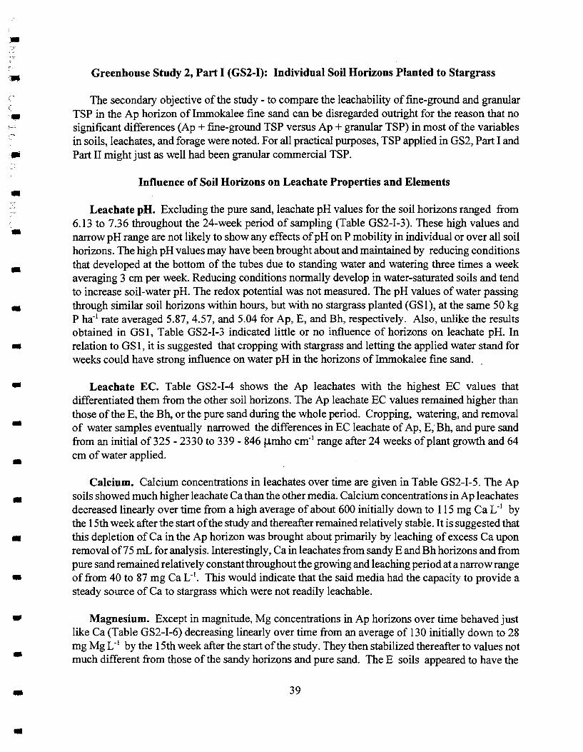
... ,...,
•
-•
•
-.. -•
•
•
•
•
•
-•
Greenhouse Study 2, Part I (GS2-I): Individual Soil Horizons Planted to Stargrass
The secondary objective of the study - to compare the leachability of fine-ground and granular TSP in the Ap horizon of Immokalee fine sand can be disregarded outright for the reason that no significant differences (Ap + fme-ground TSP versus Ap +granular TSP) in most of the variables in soils, leachates, and forage were noted. For all practical purposes, TSP applied in GS2, Part I and Part II might just as well had been granular commercial TSP.
Influence of Soil Horizons on Leachate Properties and Elements
Leachate pH. Excluding the pure sand, leachate pH values for the soil horizons ranged from 6.13 to 7.36 throughout the 24-week period of sampling (Table GS2-I-3). These high values and narrow pH range are not iikely to show any effects of pH on P mobility in individual or over all soil horizons. The high pH values may have been brought about and maintained by reducing conditions that developed at the bottom of the tubes due to standing water and watering three times a week averaging 3 em per week. Reducing conditions normally develop in water-saturated soils and tend to increase soil-water pH. The redox potential was not measured. The pH values of water passing through similar soil horizons within hours, but with no stargrass planted (GS 1 ), at the same 50 kg P ha·1 rate averaged 5.87, 4.57, and 5.04 for Ap, E, and Bh, respectively. Also, unlike the results obtained in GSI, Table GS2-I-3 indicated little or no influence of horizons on leachate pH. In relation to GS 1, it is suggested that cropping with stargrass and letting the applied water stand for weeks could have strong influence on water pH in the horizons of Immokalee fine sand. _
Leachate EC. Table GS2-I-4 shows the Ap leachates with the highest EC values that differentiated them from the other soil horizons. The Ap leachate EC values remained higher than those of theE, the Bh, or the pure sand during the whole period. Cropping, watering, and removal of water samples eventually narrowed the differences in EC leachate of Ap, E; Bh, and pure sand from an initial of325- 2330 to 339-846 J.lmho cm·1 range after 24 weeks of plant growth and 64 em of water applied .
Calcium. Calcium concentrations in leachates over time are given in Table GS2-I-5. The Ap soils showed much higher leachate Ca than the other media. Calcium concentrations in Ap leachates decreased linearly over time from a high average of about 600 initially down to 115 mg Ca L-1 by the 15th week after the start of the study and thereafter remained relatively stable. It is suggested that this depletion of Ca in the Ap horizon was brought about primarily by leaching of excess Ca upon removal of7 5 mL for analysis. Interestingly, Cain leachates from sandy E and Bh horizons and from pure sand remained relatively constant throughout the growing and leaching period at a narrow range of from 40 to 87 mg Ca L-1
• This would indicate that the said media had the capacity to provide a steady source of Ca to stargrass which were not readily leachable.
Magnesium. Except in magnitude, Mg concentrations in Ap horizons over time behaved just like Ca (Table GS2-I-6) decreasing linearly over time from an average of 130 initially down to 28 mg Mg L-1 by the 15th week after the start of the study. They then stabilized thereafter to values not much different from those of the sandy horizons and pure sand. The E soils appeared to have the
39

~ 0
I I
Table GS2-I-3. pH ofleachates from potted horizons oflmmokalee fine sand, a Spodosol, and from pure sand fertilized at 50 kg P ha·1
using fine-ground TSP, unless indicated otherwise, and planted to stargrass.
Week from first (second) P aoolication
Horizon (Treatment) 0 1 3 6 9 12 15(1) 18(4) 21(7) 24(10)
---------------------------------------------------- pH --------------------------------------------------------------------
Ap 6.85b# 7.29ab 6.85b 7.13a 7.36ab 7.40ab 7.25ab 6.90cb 7.04b 6.79ab Ap (granular TSP) 6.96b 7.07abc 6.60b 6.88ab 6.96b 7.18abc 7.23ab 7.15ab 7.16ab 6.87ab E 6.24b 6.36bc 6.93b 6.13b 6.83b 6.79c 7.00bc 7.25ab 7.05b 6.77ab Bh 6.93b 6.20c 7.07b 6.78ab 7.11ab 7.00ab 6.61c 6.56c 6.19c 6.43b Pure sand 7.82a 7.58a 7.68a 7.67a 7.69a 7.56a 7.61a 7.61a 7.64a 7.34a
Statistics: P(Horizons) < 0.01 0.04 < 0.01 0.03 0.08 < 0.01 0.02 0.01 <0.01 0.17
#Means within collection having the same letter are not different at P = 0.05 using Duncan's multiple range test.
I • I I I I I I I I I I I I I 1 I

I I
~ ......
I I I I I I I I I • I I .... - '.: I I ' •.. ; 'i ., '·.:i.;'l' . '
Table GS2-I -4. Electrical conductivity (EC) ofleachates from potted horizons oflmmokalee fine sand, a Spodosol, and from pure sand fertilized at 50 kg P ha-1 using fine-ground TSP, unless indicated otherwise, and planted to stargrass.
Week from first (second) P application
Horizon (Treatment) 0 1 3 6 9 12 15(1) 18(4) 21(7) 24(10)
---------------------------------------------------- ~mho cm-1------------------------------------------------------------
Ap. 2330a# 1182a 1657a 1036a 86la 635ab 643ab 670ab 704ab 640b Ap (granular TSP) 2217a 1324a 1935a 1115a 973a 790a 806a 886a 888a 846a E 895b 500b 714b 440b 342b 429b 372c 338c 283c 339d Bh 500c 503b 531b 489b 473b 472b 511bc 509bc 492bc 532bc Pure sand 325d 456b 377b 486b 496b 477b 505bc 498bc 491bc 469cd
Statistics: P(Horizons) <0.01 <0.01 <0.01 < 0.01 < 0.01 0.01 <0.01 <0.01 <0.01 <0.01
#Means within collection having the same letter are not different at P = 0.05 using Duncan's multiple range test.
I
Table 082-1-5. Ca concentrations in leachates from potted horizons oflmmokalee fine sand, a Spodosol, and from pure sand fertilized at 50 kg P ha·1 using fine-ground TSP, unless indicated otherwise, and planted to stargrass.
Horizon (Treatment)
Ap Ap (granular TSP) E Bh
Week from first (second) P application
0 1 3 6 9 12 15(1) 18(4) 21(7) 24(10)
---------------------------------------------------- mg ~-t --------------------------------------------------------------
631.6a# 400.6a 319.3a 225.7a 177.5a 146.4a 113.7a 144.1a 136.3ab 120.1ab 559.8a 479.2a 344.6a 257.6a 176.7a 173.4a 116.1a 142.8a 152.5a 157.5a
60.7b 53.9b 76.1b 66.5b 47.5b 77.2b 59.1b 54.1a 50.5c 49.8c 40.0b 52.0b 56.9b 53.1b 48.4b 52.5b 55.8b 73.1a 63.9bc 57.0bc
.t>. Pure sand 27.1b 57.6b 71.4b 51.8b 78.5b 86.8b 54.2b 53.6a 59.0c 64.5bc N
Statistics: P(Horizons) < 0.01 < 0.01 < 0.01 < 0.01 0.02 < 0.01 < 0.01 0.15 0.03 0.01
#Means within collection having the same letter are not different at P = 0.05 using Duncan's multiple range test.
• I I I I I I I I I I I I I I ' I I

I I I I I I I I • I I I I I , :,,, I :: < •... ' ... ,.·. .• ·;;; :· .. ' \.
Table GS2-1-6. Mg concentrations in leachates from potted horizons oflmmokalee fine sand, a Spodosol, and from pure sand fertilized at 50 kg P ha-1 using fine-ground TSP, unless indicated otherwise, and planted to stargrass.
Horizon (Treatment)
Ap Ap (granular TSP) E Bh
Week from first (second) P aoolication
0 1 3 6 9 12 15(1) 18(4) 21(7) 24(10)
---------------------------------------------------- mg ~-I--------------------------------------------------------------
141.8a# 72.2a 56.7a 44.2a 36.0a 27.5ab 24.4ab 31.0ab 29.4ab 29.1ab 121.1a 86.9a 63.3a 52.1a 40.6a 36.1a 31.4a 37.6a 36.0a 37.3a
7.4b 5.4b 7.6b 5.6c 4.2c 5.9d 5.4c 5.3c 5.3c 5.6c 15.1b 22.5b 24.2b 22.6b 21.1b 22.8bc 23.8ab 25.2ab 27.8ab 28.2ab
.~:>. Pure sand 5.9b 8.0b 13.4b 12.4bc 13.9bc 16.2cd 15.8b 16.2bc 16.4b 14.5bc w
Statistics: P(Horizons) < 0.01 < 0.01 < 0.01 < 0.01 < 0.01 < 0.01 < 0.01 0.01 0.01 < 0.04
#Means within collection having the same letter are not different at P = 0.05 using Duncan's multiple range test.

least CA. Like Ca, depletion ofMg could have been brought about primarily by leaching of excess Mg. Like Ca, Mg in leachates from sandy soil horizons and from pure sand remained relatively constant through the growing and leaching period at a narrow range of from 6 to 28 mg Mg L·1
indicating that the said media had the capacity to provide a steady source of Mg to stargrass.
Potassium. Potassium in Ap also decreased almost linearly over time from an average of 133 initially down to 21 mg K L·1 by the last sampling (Table G82-I-7). There is, however, no logical reasons why such differences should be attributed to the differences in the particle size ofTSP. The depletion of K in the Ap leachates could be primarily attributed to the leaching of excess K upon leachate withdrawal for analysis and to a lesser degree to crop removal. Potassium fertilizer was applied to all pots twice, the first at the beginning of the study and the second on the 14th week. The latter application appeared to have made no difference to K concentrations in leachates indicating that it was being utilized by the plant.
Aluminum. Table GS2-I -8 shows Al concentrations over time. The Allevels in Ap and in pure sand leachates were well defined, in Ap sharply decreasing over time up to the 12th week from an initial value of about 1.4 and stabilizing to 0.4 and 0.6 mg L-1 thereafter. This could be due primarily to leaching of excess AI upon removal of soil water for analysis. The lowest AI concentrations were in pure sand leachates which remained steady throughout at about 0.2 mg L-1
• Aluminum concentrations in Bh leachates varied widely throughout the sampling period as did AI levels in E leachates up to the 12th week. No explanation is suggested except analytical variability.
Iron. Iron concentrations were higher in E (initially, 1st, 3rd, and 9th week) and in Bh (1st, 9th and 12th week) leachates than in Ap or in pure sand (Table G82-I-9). There was little to indicate what the effects of cropping and leaching were on Fe concentrations in leachates because of its very low concentrations.
Nitrate. Nitrogen was applied to the pots as ammonium nitrate fertilizer. The differences in N03 concentrations in leachates from the various potted horizons and pure sand shown in Table G82-I-1 0 indicated that the applied amount represented but a small fraction of soil nitrate in the Ap horizon. This amount was barely detectable in the E, Bh, and in pure sand. Like the cationic nutrients, nitrate linearly decreased from an initial average value of291 mg N03 L-1 down to zero or undetectable level by the 9th week of plant growth and watering. Nitrate values went up on the 21st and the 24th after the second N application made on the 14th week. Because of extreme analytical variability, however, values as high as 74 mg N03 L-1 were not differentiable statistically from zero (Table G82-I-10).
Sulfate. No sulfate fertilizer was used in the study so that the amounts ofS04 shown in Table G82-I-11 can only be soil 804• Again, the analytical variability was extremely high so that values 3 and 216 mg L-1 (18th week) were not statistically differentiable. Like nitrate, 804 in Ap leachates also decreased over time from 883 initially down to 59 mg S04 L-1 by the 15th week. Sulfate concentration appeared to be stable in the sandy horizons and in pure sand throughout the period.
44
-.. -•
•
--•
-• •
•
•
-•
--•
I I I • I I I I I I I • I • '.•; I T ' ' ~.· ' T 'I ' ··--·
Table GS2-I-7. K concentrations in leachates from potted horizons oflmmokalee fine sand, a Spodosol, and from pure sand fertilized at 50 kg P ha-1 using fine-ground TSP, unless indicated otherwise, and planted to stargrass.
Horizon (Treatment)
Ap Ap (granular TSP) E Bh _
Week from first (second) P application
0 1 3 6 9 12 15(1) 18(4) 21(7) 24(10)
---------------------------------------------------- mg ~-~--------------------------------------------------------------
146.0a# 73.2a 54.7a 55.4a 39.3ab 28.5b 27.4b 26.9bc 20.0bc 13.1b 118.5a 77.2a 60.0a 60.la 51.9a 49.0a 52.8a 38.8b 39.0b 30.0a 47.1b 29.0b 20.7b 16.4b 10.4c 9.4ab 7.4bc 5.2bc 3.7c 2.6c 22.7bc 27.9b 25.3b 27.2b 25.6b 23.6b 22.0bc 26.9bc 11.8c 11.1bc
~ Pure sand 1.8c 1.7c 1.7c 0.6c 1.2c 1.2c 1.8c 2.0c 1.9c 1.3c Ul
Statistics: P(Horizons) < 0.01 < 0.01 < 0.01 < 0.01 < 0.01 < 0.04 < 0.03 0.13 0.01 0.04
# Means within collection having the same letter are not different at P = 0.05 using Duncan's multiple range test.
i,'•.: '···
I
Table GS2-I-8. AI concentrations in leachates from potted horizons oflmmokalee fine sand, a Spodosol, and from pure sand fertilized at 50 kg P ha·1 using fine-ground TSP, unless indicated otherwise, and planted to stargrass.
Horizon (Treatment)
Ap Ap (granular TSP) E Bh
Week from first (second) P application
0 1 3 6 9 12 15(1) 18(4) 21(7) 24(10)
---------------------------------------------------- mg ~-t --------------------------------------------------------------
1.46a# 1.03a 0.83a 0.64a 0.52a 0.49b 0.35b 0.44ab 0.45b 0.38bc 1.34a 1.18a 0.94a 0.72a 0.52a 0.54ab 0.35b 0.59a 0.50b 0.50b 0.53b 0.55b 0.85a 0.69a 0.36ab 0.36b 0.24b 0.23ab 0.24b 0.23cd 0.32c 0.53b 1.28a 0.72a 0.49ab 0.84a 0.75a 0.63a 1.19a 0.92a
~ Pure sand 0.08c 0.20c 0.22b 0.19b 0.24b 0.28b 0.17b 0.18b 0.21b 0.14d 0'1
Statistics: P(Horizons) < 0.01 < 0.01 0.04 0.08 0.13 0.02 < 0.01 0.08 < 0.01 < 0.01
#Means within collection having the same letter are not different at P = 0.05 using Duncan's multiple range test.
I I • I I I I I • I • I I I I I I I

II I I • • I I I 1 • I I I j ~ VJ J ::. ' ...•.. ''I ., ..•
Table GS2-I-9. Fe concentrations in leachates from potted horizons oflmmokalee fine sand, a Spodosol, and from pure sand fertilized at 50 kg P ha· 1 using fine-ground TSP, unless indicated otherwise, and planted to stargrass.
Horizon (Treatment)
Ap Ap (granular TSP) E Bh
~ Pure sand -...)
Statistics: P(Horizons)
Week from first (second) P application
0 1 3 6 9 12 15(1) 18(4) 21(7) 24(10)
---------------------------------------------------- mg r_-1 --------------------------------------------------------------
0.03b# 0.06c 0.06bc 0.07a 0.24bc 0.26b 0.23a 0.19a 0.17a Q,cl9a 0.02b 0.02c 0.05bc 0.09a 0.19c 0.41ab 0.22a 0.21a 0.22a 0.17a 0.41a 0.43b 0.66a 2.53a 2.44a 0.34ab 0.6la 0.46a 0.28a 0.42a 0.06b 0.77a 0.21b 0.62a 1.14b 0.9la 0.45a 0.45a 0.32a 0.53a O.OOb 0.02c O.Olc O.Ola 0.02c O.Olb 0.03a 0.04a 0.03a O.OOa
< 0.01 < 0.01 <0.01 0.25 < 0.01 0.06 0.44 0.40 0.32 0.18
# Means within collection having the same letter are not different at P = 0.05 using Duncan's multiple range test.

~ 00
II I
Table GS2-I-10. Nitrate concentrations in leachates from potted horizons oflmmokalee fine sand, a Spodosol, and from pure sand fertilized at 50 kg P ha-1 using fine-ground TSP, unless indicated otherwise, and planted to stargrass.
Week from first (second) P application
Horizon (Treatment) 0 1 3 6 9 12 15(1) 18(4) 21(7) 24(10)
---------------------------------------------------- mg r_-t --------------------------------------------------------------
Ap 355.45a# 86.27b 0.08a 10.48ab 0.16a O.OOa 0.52a 0.04b 47.00a 26.26a Ap (granular TSP) 227.06a 177 .82a 42.33a 20.92a O.OOa O.OOa O.OOa O.OOb 73.94a 48.69a E 42.83b 13.60b 0.34a 9.63ab 0.16a O.OOa 0.16a 1.83a 0.87a 0.59a Bh _ 0.32b 0.25b 0.08a 0.17b O.OOa O.OOa O.OOa O.Olb 0.29a 0.17a Pure sand 0.21b 0.21b O.OOa O.OOb O.OOa O.OOa O.OOa O.OOb O.OOa O.OOa
Statistics: P(Horizons) < 0.01 <0.01 <0.01 0.15 0.58 - 0.10 0.04 0.57 0.56
#Means within collection having the same letter are not different at P = 0.05 using Duncan's multiple range test.
I • I I I I J • I I • I I •• I I I

I I • I • I I I I • I • I . ,_- ~\' -' '·-' ,_.,-:. . I . ·'i' -,; i '''•
Table GS2-1-11. Sulfate concentrations in leachates from potted horizons oflmmokalee fine sand, a Spodosol, and from pure sand fertilized at 50 kg P ha-1 using fine-ground TSP, unless indicated otherwise, and planted to stargrass.
Horizon (Treatment)
Ap Ap (granular TSP) E Bh
.J:>. Pure sand 1.0
Statistics: P(Horizons)
Week from first (second) P application
0 1 3 6 9 12 15(1) 18(4) 21(7) 24(10)
---------------------------------------------------- mg r.-1 --------------------------------------------------------------
953a# 857ab 737a 57la 275a 223a lOlbc 12la 98ab 4a 812a 1388a 833a 697a 290a 50 a 16c 216a 142ab 109a 37lb 240b 208b 212b lOla 249a 122ab 106a 98ab 94a 136c 186b 215b 192b 164a 199a 220a 149a 274a 163a
lOc 28b 55b 55b 51 a 29a llc 3a 2b 2a
< 0.01 0.02 < 0.01 < 0.01 0.55 0.19 < 0.01 0.30 0.06 0.27
#Means within collection having the same letter are not different at P = 0.05 using Duncan's multiple range test.

Chloride. Chloride was applied to the pots as KCl. From the values in pure sand, the applied Cl represented but a small fraction of Cl in the Ap horizon (Table GS2-I-12). Chloride in Ap leachates decreased very gradually over time down to the last sampling but appeared to be stable in the other soil horizons and in pure sand. The pure sand and the E horizon leachates had the least amounts of chloride.
Phosphorus in Leachates
Leachate P concentrations overtime are given in Table GS2-I-13. Leachate P concentrations in both potted Ap soils differed only on the 9th and the 12th week of sampling. The results indicated that grinding the commercial granular TSP to powder made no difference in P solubility in soil.
Unlike the major cationic or anionic plant nutrients discussed earlier which decreased in concentrations with time, P in leachates remained relatively constant in each medium over time (Table GS2-I-13). Table GS2-I-13 also shows that P concentrations in the Ap leachates remained very much higher than those in E, Bh, or pure sand leachates, and these even increased after the second P fertilizer application particularly by the 24th week. These showed that the amounts of readily available soil P in the Ap horizon of Immokalee fine sand were simply far in excess of stargrass's needs for P. On the other hand, the very small amounts ofP that leached through E, Bh, and pure sand would imply that stargrass utilized most ofthe fertilizer P and demonstrated pasture cropping as the major method or practice to prevent P losses through leaching and, possibly, also runoff. By the 24th week, almost nothing leached from Bh and pure sand.
Relations Between Phosphorus and Some Leachate Properties and Elements
Leachate pH and P. There was no relation (Table GS2-I-14) between leachate pH and P concentrations within the pH range 6.13 to 7. 82. Labile inorganic P in soils is relatively high at this pH range or between pH 6.0 and 7.0 (Buckman and Brady, 1970; Sharpley, 2000).
Leachate EC and P. Leachate EC was strongly positively correlated with P concentrations in leachates (Table GS2-14). This would indicate that P tended to be highly mobile in soil-water high in salt concentrations as noted in GS 1.
Leachate cations and P. Individually, all major cations were associated positively with P concentrations particularly Ca, Mg, and K (Table GS2-I-14; GSl). This would indicate that ionpairing between the dissolved anionic P species such as P04·, HP04, and H2P04 and the cations give P its mobility in the soil.
No significant association between AI and Fe with Pin leachates were noted (Table GS2-I-14). This was likely due to the low solubility of these materials in the pH range just noted. Although not significant, Fe tended to be negatively associated with P concentrations. This was also observed in GS 1 using the same or similar soils with no stargrass planted. Low dissolved Fe in leachates would mean low Fe precipitates in equilibrium with dissolved Fe and low potential capacity to tie up P, thus the higher P concentrations at the lower Fe concentrations or the negative association.
50
•
•
•
•
•
-•
•
•
•
•
-•
•
•
-•

I •
Ul 1-'
I I I J I I 'I I I f I I , t.: a· , . , ,. -c ,.i:.:: ,·, ;:l:; ''•' i'' '''il '
Table GS2-I-12. Chloride concentrations in leachates from potted horizons oflmmokalee fine sand, a Spodosol, and from pure sand fertilized at 50 kg P ha·1 using fine-ground TSP, unless indicated otherwise, and planted to stargrass.
Week from first (second) P application
Horizon (Treatment) 0 1 3 6 9 12 15(1) 18(4) 21(7) 24(10)
---------------------------------------------------- mg r_-I --------------------------------------------------------------
Ap 140a# 56ab 47a 39a 33a 30ab 33ab 29ab 2lab 14a Ap (granular TSP) 112a 93a 55 a 44a 40a 40a 47a 4la 33a 27a E 23b 12b llb 9b 9b lOb 12b 13b 9b 7a Bh 36b 42ab 41a 38a 41a 38a 44a 40ab 23ab 22a Pure sand 5b 5b 6b 7b 9b 9b 12b 13b llab lOa
Statistics: P(Horizons) <0.01 0.03 <0.01 < 0.01 <0.01 0.02 0.03 0.05 0.17 0.18
#Means within collection having the same letter are not different at P = 0.05 using Duncan's multiple range test.
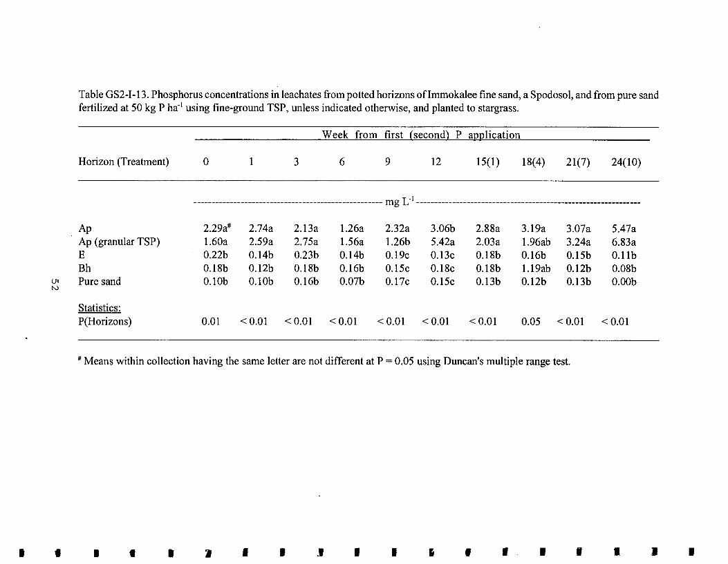
I
Table GS2-I -13. Phosphorus concentrations in leachates from potted horizons oflmmokalee fine sand, a Spodosol, and from pure sand fertilized at 50 kg P ha·• using fine-ground TSP, unless indicated otherwise, and planted to stargrass.
Horizon (Treatment)
Ap Ap (granular TSP) E Bh
Week from first (second) P aoolication
0 1 3 6 9 12 15(1) 18(4) 21(7) 24(10)
---------------------------------------------------- mg ~-· --------------------------------------------------------------
2.29a# 2.74a 2.13a 1.26a 2.32a 3.06b 2.88a 3.19a 3.07a 5.47a 1.60a 2.59a 2.75a 1.56a 1.26b 5.42a 2.03a 1.96ab 3.24a 6.83a 0.22b 0.14b 0.23b 0.14b 0.19c 0.13c 0.18b 0.16b 0.15b O.llb 0.18b 0.12b 0.18b 0.16b 0.15c 0.18c 0.18b 1.19ab 0.12b 0.08b
lJ1 Pure sand 0.10b O.lOb 0.16b 0.07b 0.17c 0.15c 0.13b 0.12b 0.13b O.OOb N
Statistics: P(Horizons) 0.01 < 0.01 < 0.01 < 0.01 < 0.01 < 0.01 <0.01 0.05 < 0.01 < 0.01
#Means within collection having the same letter are not different at P = 0.05 using Duncan's multiple range test.
• I • I J I I .I I I i • I I I I I I

'•
-----.. -•
•
•
•
•
•
Table GS2-I -14. Relationships between P concentrations (Y = mg P/unit X) and pH, EC, cation, and anions (X) in leachates from all potted media (Ap, E, and Bh horizons of Immokalee fine sand and from pure sand) planted to stargrass and fertilized twice at 50 kg P ha·1
•
Leachate variable Unit Regression equation P-level#
Gross nronertv: pH y = - 0.043X + 1.56 0.00 ns EC j..Lmho cm·1 y = 0.002X + 0.18 0.18 **
Macro cations: mgL-1
Calcium y = 0.005X + 0.54 0.20 *** Magnesium y 0.025X + 0.52 0.19 ** Potassium y 0.022X + 0.62 0.16 **
Micro cations: mgL-1
Aluminum y = 0.823X + 0.80 0.03 ns Fe y = - 0.698X + 1.50 0.05 ns
Macro anions: mgL-1
Sulfate (S04) y = 0.001X + 0.98 0.04 ns Chloride (Cl) y = 0.197X + 0.65 0.10 * Nitrate (N03) y = 0.007X + 1.09 0.08 *
#ns =not significant at P = 0.05, *significant at P = 0.05, **significant at P = 0.01, ***significant at P .:S 0.001.
Leachate anions and P. Anions Cl and N03 were supplied to the potted soils as KCl and NH4N03 but no S04. All the anions tended to be positively associated with P concentrations in leachates (Table GS2-I-14). These associations might be coincidental in the sense that these anions can remain in dissolved state in the soil water only when paired with the abundant major cations like Ca, Mg, orK.
Forage Yield, Phosphorus, and Other Nutrients in Forage
Forage Yield and Percent Dry Matter. Total yields and average% DM in Table GS2-I-15 were not different for all soil horizons. Pure sand gave the lowest yield which was significantly different only from the Ap with fine-ground TSP. The potted Ap yields of 41.9 for granular and 52.5 mg por1 for fine-ground TSP were. not statistically different. On hectare-basis, forage DM yields would have ranged from 12.26 Mg for sand to and average of 15.03 Mg for the two Ap's.
53

Phosphorus and other nutrients in forage. The two applications ofP fertilizers totaled 314.0 mg por1• The P uptake values for the plants in the two Ap soils computed from dry matter yields, averaged 132.0 mg por1 or 42.0% of the applied fertilizer P {Table GS2-I-15). The P uptake by plants in E, Bh, and pure sand averaged 34. 7, 36.3, and 33.4% of the applied P, respectively, which were not statistically different from one another and, most likely, are not different from the lower P. uptake value of 34.7 % for Ap plants fertilized with granular TSP. Thus, despite the different amounts of available P among the various media {Tables GS2-I-2 and GS2-I-16), P uptake by stargrass was limited to a narrow range of0.27 to 0.29% Pin the tissue. This would mean that soils planted to stargrass having 0.27 to 0.29% P with no P fertilizer do not need any fertilizer P, and any application of P would just be a waste of money since it is not likely to increase forage yield but would most likely increase P losses through leaching and/or runoff {Table GS2-I-13).
Higher tissue K contents were not strongly associated with increased yields. Iron, Cu, Zn, and Mn uptakes were very similar for all soil horizons and for pure sand (Table GS2-I-15). Since pure sand was not supposed to have as much of these macro and micro nutrients as the soil horizons, their sources in the potted pure sand could have been the rich top soil in the sods or swards. It appeared then that there were enough Ca, Mg, and the micro nutrients in the top two inches of soil of Immokalee fine sand to meet the needs of stargrass.
Phosphorus and Other Nutrients in Soil
The pre-treatment analyses of Ap, E, and Bh horizons {Table GS2-I-l) indicated that_ the Bh horizon was much richer in plant nutrients than the Ap horizon except for Fe. TheE horizon, being primarily sand, had the least amounts of plant nutrients among the three soil horizons. At the end of the study the soils were analyzed again to determine the changes that had occurred after cropping with stargrass. The sod was separated from the soil column, and the sod soil was analyzed separately.
Soil Column. Although no statistical analysis was done to compare pre- and post-treatment values, some notable changes appeared to have occurred (Table GS2-I-16). The pH values of potted Ap and E horizons, but not that of the Bh, appeared to have increased due, probably, to the loss of acidic substances from these horizons because ofleaching. The almost unchanged pH ofthe Bh rules out the effect of submergence, which tended to increase soil pH, since the Bh tended to remain moist for longer periods than the Ap or the E due to the standing water. This then could be due to the strong buffering capacity of the Bh horizon at the pH range 4.8 - 5.0 as reported in GSl.
Phosphorus appeared to have build up in the Ap soils after P fertilization averaging 15.0 mg kg·1
compared to the pre-fertilization value of 2.0 mg kg·1• It is possible, however, that the low pre
fertilization value for the Ap soil was simply an analytical anomaly. More will be said about these pre- and post-fertilization P values in accounting for fertilizer P. TheE soils ended up with the same pre- and post fertilization P values of 1.2 (Table GS2-I-1) and 1.3 mg kg-1 (Table GS2-I-16). The applied P could be accounted for by P taken up by the plant, in leachates withdrawn for analysis, retained in the soil column, and in the sod soil {Table GS2-I-16). It was unfortunate that no prefertilization analysis of the sod soil was done or that no P control was included in the treatments at least for the Ap soil. The Bh continued to have the highest amount of extractable P.
54
---•
•
•
•
-•
•
•
---•
•
-•
•

I I
Ul Ul
I I I I I I I I I I I I --.
:<'O .-;· <- ,-·, :~ ; .•.... 'I', 1 <.•.:. <'I
Table GS2-I-15. Total dry matter (DM) yield, percent dry matter (%DM), and total elemental uptake by stargrass planted in potted Ap, E, and Bh horizons oflmmokalee fine sand, a Spodosol, and in pure sand fertilized at 50 kg P ha-1 applied twice using fine-ground TSP, unless indicated otherwise.
Elemental uotake
Horizon (Treat.) %DM DM p K Ca Mg Fe Al Cu Zn Mn
gpor1 ------------------------------------------- mg por1 -------------------------------------------------------
Ap 27.4a 52.5a# 155a 479a 389a 143a 2.71a 266a 0.55a 2.35a 1.85a Ap (granular TSP) 24.1 a 41.9ab 109b 452a 248b 97b 2.12a 318a 0.40a 2.06a 1.13a E 29.7a 40.2ab 109b 326b 324ab 113ab 3.05a 467a 0.45a 1.91a 1.45a Bh 28.2a 42.6ab 114b 453a 292ab 118ab 2.66a 342a 0.45a 2.16a 1.44a Pure sand 27.0a 38.5b 105b 333b 277ab 116ab 2.63a 410a 0.49a 2.02a 1.54a
Statistics: P(Horizons) 0.41 0.18 0.04 < 0.01 0.12 0.15 0.70 0.61 0.44 0.94 0.32
#Means with same letter are not different at P = 0.05 using Duncan's multiple range test.

Table GS2-I-16. Soil pH and certain Mehlich I extractable elements in potted soil horizons of Immokalee fine sand and in pure sand planted to stargrass and fertilized twice at 50 kg P ha-1 with the second P application made 14 weeks after the first.
Horizon pH p K Ca Mg Fe
------------------------------- mg kg-1-------------------------------
Ap 6.1b# 12.9b 5.2ab 1195b 72.0b 7.9bc Ap (granular) 6.0b 17.1b 8.8a 1323a 86.7a 8.7a E 5.3c 1.3c 0.4c 36d 4.0c 4.4bc Bh 5.0d 92.3a 4.0bc 573c 90.7a 3.7c Pure sand 6.5a 2.4c 0.4c 28d 2.7c 4.3c Statistics: P(horizon) <0.01 <0.01 <0.01 <0.02 <0.01 0.07
Sod soil: Ap 5.3a 28.3a 16.0a 1759a 256a 3.2a Ap(granular) 5.3a 16.7a 21.9a 2076a 345a 3.5a E 5.2a 31.9a 16.3a 1456a 257a 4.0a Bh 4.8a 28.9a 18.8a 1245a 229a 4.5a Pure sand 5.1a 24.9a 17.6a 1517a 285a 5.3a Statistics: P(horizon) 0.61 0.64 0.75 0.80 0.91 0.68
#Means with same letter are not different at P = 0.05 using Duncan's multiple range test.
For the other nutrients, theE and the.pure sand had the lowest amounts ofK, Ca, and Mg (Table GS2-I -16). Between the pre- and the post-fertilization, K remained almost unchanged in the Ap and was substantially reduced in the E and the Bh soils. Extractable Ca and Mg were substantially increased in the Ap but remained almost unchanged in the Bh. Iron was unchanged in the Ap, E, or the Bh soils.
Sod Soil. Table GS2-I-16 shows no significant differences in sod soil pH or any of the plant nutrients between any two potted soil horizons of Immokalee fine sand and pure sand. This would indicate that similar amounts of any one particular nutrient analyzed were taken up by the plant and/or lost from the sod soil with leaching.
56
---•
•
•
--•
•
----•
-•
-•

. , ,. :-.
•
-•
•
•
-•
-•
.. •
.. --
Accounting for Soil and Fertilizer Phosphorus
The summary for Pin the above-ground plant tissue (roots and the stubble portions were not analyzed), in leachate withdrawn for analysis, and in soil column and in sod soil is given in Table GS2-I-17. Total Pin leachates was the sum ofthe products ofthe volumes and concentrations for ten samplings done during the period of study .
Table GS2-I -1 7. Accounting for P in soil horizons oflmmokalee fine sand and in pure sand planted to stargrass and fertilized twice at 50 kg P ha-1 with the second P application made 14 weeks after the first.
Potted growing media P Source Aphorizon E horizon Bh horizon Pure sand
Fertilizer P +initial soil P: ------------------------Total mg P por1 (%) -----------------------------
Fertilizer P applied 314.0 (90.60) 314.0 (91.12) 314.0 (19.78) 314.0 (96.17) Initial soil P in colwnn 21.2 ( 6.12) 14.7 ( 4.27) 1,258.9 (79.31) 0.0 ( O.OOl
Sod soil## 11.3 ( 3.26) 15.9 ( 4.61) 14.5 ( 0.91) 12.5 ( 3.83) Initial-Total 346.5 (I 00.0) 344.6 (100.0) 1,587.4 (100.0) 326.5 (1 00.0)
Post fertilization P sources: Plant tissue 132.0 (43.32) 109.0 (77.36) 114.0 ( 9.05) 105.0 (71.43) Leachate withdrawn 2.2 ( 0.72) 0.1 ( 0.07) 0.2 ( 0.02) 0.1 ( 0.07) Soil column 159.2 (52.25) 15.9 (11.28) 1,130.3 (89.78) 29.4 (20.00) Sod soil 11.3 ( 3.62) 15.9 (11.28) 14.5 ( 1.15) 12.5 ( 8.50) Post-Total 304.7 (1 00.0) 140.9 (100.0) 1,259.0 (100.00) 147.0 (100.0)
---------------------------- post-P :pre-P ratio ----------------------------
Soil: post-P:pre-P ratio 7.51 [1.05]### 1.08 0.90
Total: post-P:pre-P ratio 0.88 [0.78]### 0.41 1.26 0.45
# Zero P was assumed since no analysis of pure sand was done prior to planting and P fertilization . tmv alues are those after the study using an amount of sod soil of about 500 g; no analysis of soil in
sod was done prior to planting and P fertilization. Estimated values are intended to show the very high P concentrations in sod soil (Table GS1-I-15) in proper perspective.
~sing the value for Ap in Table GS1-3 as discussed in the text .
57

Fertilizer P applied to each pot ranged from about 20% of the total Pin Bh soils to 96% in pure sand. The Ap and the E had almost similar initial P concentrations of 2.0 and 1.2 mg kg·1
( Table GS2-I-1), respectively. The value for Ap appeared unreasonable low. For portions of the same or similar soils, Table GS 1-3 showed the Ap and the E horizons to have initial P concentrations of 14.2 and 0.9 mg P kg·1
• Using 14.2 mg P kg·1 for Ap for the present study would result to a total P of 150.7 mg por1 instead of just 24.5 mg por1 shown in Table GS2-I-17. Then the initial total and the post-fertilization total of 476.0 and 304.7 mg P por1
, respectively, would be more reasonable. Because the choice of value to use for Ap would affect the interpretation of the data, it is not unreasonable to use the value obtained in Table GSI-3 for the same or similar soil. Not to do otherwise would force us to conclude that the post-study soil P concentration increased 7.5 times that of pre-study P concentration which cannot be explained without resorting to claims of increased soil P mobilization in the Ap upon P fertilization.
Using the pre-fertilization P concentration value of Table GSI-1-3 for Ap soil suggested above, the data indicated that the potted Ap, E, and Bh soil horizons contained as much P after the study as was present initially, with soil pre-P:post-P ratios of 1.06, 1.08, and 0.90, respectively (Table GS2-I-17). This would indicate that the stargrass plant took up almost the same amount ofP in each potted medium, and this was supported by the P uptake (Tables GS2-I-15). That this was indeed the case was supported also by the leachate P data which showed almost no loss ofP forE, Bh, and pure sand. The greater loss ofP from the Ap could be attributed to amounts ofP in excess of plant needs because of the significant amounts of soil P. On percent basis, the Bh lost the least amount of P through leaching. Accounting for total P gave ratios less than 1.0 (Table GS2-I-17) due to the unaccounted P in roots and in stubbles and possible conversion of fertilizer P into non-Mehlich extractable P. Unaccounted P appeared to be highest forE horizon and for pure sand with total postP:pre-P ratios of0.41 and 0.45, respectively.
58
•
•
-•
•
--•
•
•
-•
•
-•
-•
-•

:','1
••
•
•
••
•
•
•
•
•
•
•
•
•
•
•
-•
Greenhouse Study 2, Part II (GS2-II): Reconstructed Soil Profile Planted to Stargrass
Calcium Amendments and Associated Leachate Properties
In this study, shallow well water samples were obtained at the bottom of theE horizon while those of the deep well at the bottom of the spodic horizon. The bottom leachates were samples that drained at the bottom of the PVC tubes. For convenience, all samples are simply called leachates and, at time, soil water.
It may be important to note at this point that the granular mined gypsum, the calcium carbonate, and the dolomite were all ground into fine powder for use in this study. While it was shown in GS2-I that fine-ground TSP behaved no differently from the commercial granular TSP, this may not be true in the case ofthe Ca amendments. This should be kept in mind when evaluating the effects of the Ca amendments in this study .
Leachate Ca concentration. There were no statistical differences between any two Ca amendments due, most likely, to the grinding ofthe amendments into powder (Tables GS2-II-2, GS2-II-3, and GS2-II-4). Nor were any differences noted between any amendment and the control indicating a very well limed soil. In the shallow well leachates, Ca concentrations in the control tended to be lower than in the amended leachates, but the differences did not attain a level of significance. This would mean that the amendments did add some Ca to the Ap+E profile but not enough to make any significant difference to an already well-limed field.
Leachate EC. Tables GS2-II-5, GS2-II-6, and GS2-II-7 show the statistics for each collection for the shallow wells, the deep wells, and the bottom leachates, respectively. At no instance were there any differences between any two treatments although the control tended to have lower EC than the amended ones particularly for the shallow wells. For the amendments, this would indicate that grinding them into powder obliterated the distinctive difference in solubilities between the lime materials and the gypsum which, in water at 25 °C, are 0.014, 0.320, and 2.410 g L-1 for calcium carbonate, dolomite, and gypsum, respectively (Weast, 1980-81). No doubt, this would have consequence on their effects on P mobility in soils .
Leachate pH. The pH of shallow wellleachates ranged from 6.87 to 7.09 at pre-amendment application and from 6.24 to 7.02 for the ten samplings during the 24-week period (Table GS2-II -8). These high values and narrow pH range are not likely to show any effects of pH on P mobility in individual or over all soil horizons. The high pH values may have been brought about and maintained by reducing conditions that developed in the tubes due to standing water. Reducing conditions normally develop in water-saturated soils and tend to increase soil-water pH. The redox potential was not measured. The lower post-treatment pH could be attributed to the influence of the acidic TSP. It is surprising to note that the pH values ofleachates from the control, the lime-treated, and the gypsum-treated soils were not statistically different except at one sampling (21st week) during the 24-week period. Even at this one instance, only dolomite at 4 Mg ha-1 had pH higher than the control. Consistent with what was found in GS 1, mined gypsum reduced the pH of leachates below that of the control in this one instance. In all instances, the pH values of the lime- and the
59

Table GS2-II -2. Ca concentrations in shallow wellleachates from reconstructed soil profile oflmmokalee fine sand planted to stargrass fertilized at 50 kg P ha·1 and amended with Ca amendments.
Week from first (second) P aQQlication Treatment Rate 0 1 3 6 9 12 15(1) 18(4) 21(7) 24(10)
rvig ha·1
------------------------------------------------------- mg ~-t --------------------------------------------------------
No amendment 0 125.3a# 98.0a 88.4a 82.5a 81.8a 65.8a 7l.la 67.3a 66.3a 62.7a
Gypsum 2 206.8a 157.7a 128.7a 104.1a 90.7a 74.4a 71.7a 69.5a 63.6a 59.0a 4 159.3a 134.2a 87.4a 79.2a 76.3a 61.5a 20.2a 54.8a 53.7a 64.3a
~ime_stone 2 178.6a 149.8a 108.7a 92.9a 85.3a 72.2a 71.6a 63.6a 59.4a 56.5a O'l 4 182.7a 145.9a 134.7a 105.7a 92.4a 78.3a 76.7a 69.4a 59.5a 59.3a 0
Dolomite 2 191.8a 137.7a 134.5a 111.5a 99.3a 83.5a 39.6a 77.la 72.0a 67.1a 4 161.1a 109.3a 128.0a 116.6a 99.9a 79.9a 78.4a 70.8a 63.5a 57.6a
REGRESSION: Gypsum ~inear (R2
) -## ns ### ns ns ns ns ns ns ns ns Quadratic (R2
) - ns ns ns ns ns ns ns ns ns Limestone ~inear (R2
) - ns ns ns ns ns ns ns ns ns Quadratic (R 2) - ns ns ns ns ns ns ns ns ns
Dolomite ~inear (R2
) - ns ns ns ns ns ns ns ns ns Quadratic (R2
) - ns ns ns ns ns ns ns ns ns
#rvfeans within collection having the same letter are not different at P = 0.05 using Duncan's multiple range test. ~ot determined; ~ot significant at P = 0.05.
I I I I I I I I I I I I I I I I I I I

I I I I I I I I I I I I I I . /.' •. , ; ' .;. , T .•.... .• ~. '·; ;' 'i
Table GS2-II-3. Ca concentrations in deep wellleachates from reconstructed soil profile oflmmokalee fine sand planted to stargrass fertilized at 50 kg P ha·' and amended with Ca amendments.
Week from first (second) P aQQlication Treatment Rate 0 1 3 6 9 12 15(1) 18(4) 21(7) 24(10)
1vfg ha·' ------------------------------------------------------- mg ~-' --------------------------------------------------------
No amendment 0 66.1a# 56.2a 50.7a 42.1a 35.4a 37.la 40.2a 35.4a 39.0a 37.5a
Gypsum 2 77.7a 57.1a 40.7a 36.2a 40.1a 42.7a 52.2a 42.1a 47.2a 44.9a 4 72.2a 55.6a 52.0a 58.8a 49.9a 56.5a 56.9a 49.6a 49.3a 46.6a
~imestone 2 72.6a 51.9a 42.2a 47.4a 50.1a 46.la 52.3a 46.2a 48.3a 46.7a 0'1 4 78.6a 61.2a 44.5a 47.5a 48.3a 49.0a 53.0a 43.9a 5l.Oa 50.0a ,_.
Dolomite 2 74.0a 5l.Oa 60.8a 43.0a 41.1a 45.2a 50.2a 44.1a 46.la 47.9a 4 68.9a 58.2a 64.1a 44.7a 46.4a 46.4a 45.8a 44.4a 50.5a 50.0a
REGRESSION: Gypsum ~inear (R2
) -## ns ### ns ns ns ns 0.78* ns ns ns Quadratic (R2
) - ns ns ns ns ns 0.79* ns ns ns ~imestone
~inear (R2) - ns ns ns ns ns ns ns ns ns
Quadratic (R2) - ns ns ns ns ns ns ns ns ns
Dolomite ~inear (R2
) - ns ns ns 0.77* 0.71* ns ns 0.88* 0.68* Quadratic (R2
) - ns ns ns 0.79* 0.70* ns ns 0.89* 0.69*
#Means within collection having the same letter are not different at P = 0.05 using Duncan's multiple range test. ~ot determined; ~ot significant at P = 0.05; *Significant at P = 0.05.

Table. GS2-II-4. Ca concentrations in bottom leachates from reconstructed soil profile oflmmokalee fine sand planted to stargrass fertilized at 50 kg P ha-1 and amended with Ca amendments.
Week from first (second) P annlication Treatment Rate 0 1 3 6 9 12 15(1) 18(4) 21(7) 24(10)
Mg ha-1 ------------------------------------------------------- mg L -l -----------------------------------------------------------
No amendment 0 36.1a# 32.7a 31.8a 33.7a 31.2a 35.2a 41.0a 37.6a 41.5ab 39.8bc
Gypsum 2 28.1a 28.0a 24.6a 21.4a 23.2a 30.0a 44.2a 40.6a 42.0ab 46.3ab 4 33.5a 27.4a 27.5a 27.1a 27.3a 32.0a 45.9a 35.4a 36.6b 37.7c
Limestone 2 30.4a 24.7a 22.3a 21.2a 21.6a 26.la 39.8a 32.7a 35.3b 37.5c 0'1 4 30.0a 27.1a 17.6a 18.1a 20.9a 26.2a 45.2a 34.9a 38.0ab 42.2abc N
Dolomite 2 38.0a 32.4a 29.7a 27.5a 30.8a 36.2a 47.7a 41.7a 46.0a 47.6a 4 34.7a 31.4a 22.3a 21.4a 23.4a 28.0a 38.3a 36.7a 40.1ab 44.3abc
REGRESSION: Gypsum
Linear (R2) -## ns ### ns ns ns ns ns ns ns ns
Quadratic (R2) - ns ns ns ns ns ns ns ns ns
Limestone Linear (R2
) - ns 0.71* 0.80** 0.77* 0.72* ns ns ns ns Quadratic (R2) - ns 0.75* 0.90** . 0.78* 0.72* ns ns ns ns
Dolomite Linear (R2
) - ns ns 0.78* ns ns ns ns ns ns Quadratic (R2) - ns ns 0.75* ns ns ns ns ns ns
#Means within collection having the same letter are not different at P = 0.05 using Duncan's multiple range test. ~ot determined; ~ot significant at P = 0.05; ·Significant at P = 0.05; and •• Significant at P = 0.01.
I I I I I I I I I I I I I I I I I I I
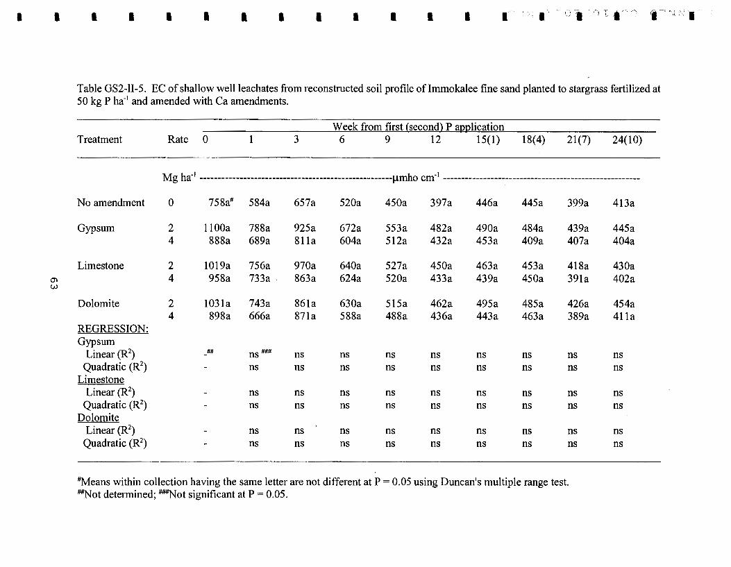
I I I I I I I I I I I I I I ' ; IT ' ; ' ~. ,· . i '; • ' .·, 'I 'i,''"l
Table GS2-II-5. EC of shallow wellleachates from reconstructed soil profile oflrnrnokalee fine sand planted to stargrass fertilized at 50 kg P ha-1 and amended with Ca amendments.
-----week from first (second) p auulication
Treatment Rate 0 1 3 6 9 12 15(1) 18(4) 21(7) 24(10)
Mg ha-1 -----------------------------------------------------1-Lmho em -l ------------------------------------------------------
No amendment 0 758a# 584a 657a 520a 450a 397a 446a 445a 399a 413a
Gypsum 2 1100a 788a 925a 672a 553a 482a 490a 484a 439a 445a 4 888a 689a 811a 604a 512a 432a 453a 409a 407a 404a
Limestone 2 1019a 756a 970a 640a 527a 450a 463a 453a 418a 430a O'l 4 958a 733a. 863a 624a 520a 433a 439a 450a 391a 402a w
Dolomite 2 1031a 743a 861a 630a 515a 462a 495a 485a 426a 454a 4 898a 666a 871a 588a 488a 436a 443a 463a 389a 411a
REGRESSION: Gypsum
Linear (R2) -## ns ### ns ns ns ns ns ns ns ns
Quadratic (R2) - ns ns ns ns ns ns ns ns ns
Limestone Linear (R2
) - ns ns ns ns ns ns ns ns ns Quadratic (R2
) - ns ns ns ns ns ns ns ns ns Dolomite
Linear (R2) - ns ns ns ns ns ns ns ns ns
Quadratic (R2) - ns ns ns ns ns ns ns ns ns
-
#Means within collection having the same letter are not different at P = 0.05 using Duncan's multiple range test. ~ot determined; ~ot significant at P = 0.05.

Table GS2-II-6. EC of deep wellleachates from reconstructed soil profile of Immokalee fine sand planted to stargrass fertilized at 50 kg P ha·' and amended with Ca amendments.
Week from first (second) P annlication Treatment Rate 0 1 3 6 9 12 15(1) 18(4) 21(7) 24(10)
Mg ha _, ---------------------------------------------------- Jlmho em·' ------------------------------------------------------
No amendment 0 575a# 544a 598a 523a 463a 433a 464a 457a 467a 476a
Gypsum 2 605a 473a 563a 426a 414a 420a 469a 455a 470a 489a 4 596a 507a 557a 482a 428a 406a 441a 453a 454a 482a
Limestone 2 564a 511a 539a 492a 459a 433a 465a 470a 488a 495a 0'1 4 631a 497a 554a 476a 451a 422a 448a 448a 468a 492a .t:>
Dolomite 2 638a 517a 574a 493a 451a 426a 477a 472a 472a 505a 4 592a 528a 573a 476a 426a 406a 431a 450a 451a 484a
REGRESSION: Gypsum
Linear (R2) -## ns ### ns ns ns ns ns ns ns ns
Quadratic (R2) - ns ns ns ns ns ns ns ns ns
Limestone Linear (R2
) - ns ns ns ns ns ns ns ns ns Quadratic (R2) - ns ns ns ns ns ns ns ns ns
Dolomite Linear (R2
) - ns ns ns ns ns ns ns ns ns Quadratic (R2
} - ns ns ns ns ns ns ns ns ns
#Means within collection having the same letter are not different at P = 0.05 using Duncan's multiple range test. ~ot determined; ~ot significant at P = 0.05.
I I I I I I I I I I I I I I I I I I I

I I I I I I I I I I I I I I . 'i •. '·- i-· ·: ' . I .. , a··, ,._ •... , ;'I
Table. GS2-II-7. EC of bottom leachates from reconstructed soil profile oflmrnokalee fine sand planted to stargrass fertilized at 50 kg P ha-1 and amended with Ca amendments.
Week from first (second) P annlication Treatment Rate 0 1 3 6 9 12 15(1) 18(4) 21(7) 24(10)
M g ha-1 -----------------------------------------------------jlmho cm-1 -------------------------------------------------------
No amendment 0 571a# 533a 548a 506a 468a 443a 458a 458a 467a 482a
Gypsum 2 574a 453a 492a 434a 403a 411a 464a 468a 467a 502a 4 549a 439a 476a 420a 395a 401a 431a 442a 452a 468a
Limestone 2 540a 452a 473a 435a 413a 413a 440a 450a 477a 484a (j) 4 557a 459a 497a 430a 418a 412a 435a 448a 457a 477a Ul
Dolomite 2 582a so2a 527a 478a 440a 435a 476a 485a 467a 509a 4 729a 464a 512a 438a 410a 401a 443a 453a 439a 484a
REGRESSION: Gypsum
Linear (R2) -## ns ### ns ns ns ns ns ns ns ns
Quadratic (R2) - ns ns ns ns ns ns ns ns ns
Limestone Linear (R2
) - ns ns ns ns ns ns ns ns ns Quadratic (R2
) - ns ns ns ns ns ns ns ns ns Dolomite
Linear (R2) - ns ns ns ns ns ns ns ns ns
Quadratic (R2) - ns ns ns ns ns ns ns ns ns
#Means within collection having the same letter are not different at P = 0.05 using Duncan's multiple range test. ~ot determined; ~ot significant at P = 0.05.

Table GS2-II-8. pH of shallow wellleachates from reconstructed soil profile oflmmokalee fine sand planted to stargrass fertilized at 50 kg P ha-1 and amended with Ca amendments.
Week from first (second) P annlication Treatment Rate 0 1 3 6 9 12 15(1) 18(4) 21(7) 24(10)
rvig lla-1
-------------------------------------------------------- pH ----------------------~-------------------------------------
No amendment 0 7.08a# 6.84a 6.80a 6.85a 6.73a 6.29a 6.58a 6.39a 6.90a 6.47a
Gypsum 2 6.91a 6.74a 6.55a 6.68a 6.66a 6.24a 6.49a 6.34a 6.54b 6.34a 4 6.98a 6.72a 6.72a 6.65a 6.64a 6.49a 6.52a 6.64a 6.36b 6.45a
Limestone 2 7.05a 6.64a 6.48a 6.75a 6.68a 6.36a 6.53a 6.41a 6.66ab 6.29a 0'1 4 6.93a 6.55a- 6.63a 6.79a 0'1
6.53a 6.31a 6.45a 6.46a 6.70ab 6.37a
Dolomite 2 6.87a 6.59a 6.73a 6.81a 6.63a 6.25a 6.51a 6.33a 6.57ab 6.3la 4 7.09a 6.71a 6.83a 6.91a 6.55a 6.26a 6.47a 6.37a 6.50b 6.39a
REGRESSION: Gypsum
Linear (R2) -## ns m ns ns ns ns ns ns 0.65** ns
Quadratic (R2) - ns ns ns ns ns ns ns 0.66** ns
Limestone Linear (R2
) - ns ns ns ns ns ns ns ns ns Quadratic (R2) - ns ns ns ns ns ns ns ns ns
Dolomite Linear (R2
) - ns ns ns ns ns ns ns ns ns Quadratic (R2
) - ns ns ns ns ns ns ns ns ns
#rvfeans within collection having the same letter are not different at P = 0.05 using Duncan's multiple range test. ~ot determined; ~ot significant at P = 0.05; **Significant at P = 0.01.
I I I I I I I I I I I I I I I I I I I

·•
;·•
•
•
•
•
•
-•
•
•
•
•
•
-•
gypsum-treated leachates were not different. In GS 1 where no stargrass was planted to the potted soils, pH of leachates defined the difference between the gypsums and the lime materials. Unfortunately, the grinding of the amendments prevented us from attributing this unexpected noneffect solely to cropping.
For the deep wells, the statistics are given in Table GS2-II-9. Six out of nine post-treatment samplings indicated no effects of amendments on pH. Of the other three, no consistent differences on treatment effects were noted.
The bottom leachates were much more acidic than the shallow or the deep wells samples (Table GS2-II-l 0). No differences in pH between any two treatments were noted in eight samplings out of nine. The one collection with differences (18th week) showed gypsum at 2 Mg ha-1 having a pH lower than that oflimestone at the same rate and no other. Again, cropping and the grinding of the amendments may have masked the distinctive difference between the gypsum and the lime materials .
Calcium Amendments and P Concentrations in Leachates
Phosphorus concentrations in leachates. Tables GS2-II-11, GS2-II-12, and GS2-II-13 for the shallow wells, deep wells, and bottom leachates, respectively, show the effects of the various Ca amendments on P in leachates. No logical significant post-application differences between treatments were not~d in all samplings at all depths. This would mean that calcium carbonate or dolomite when ground to powder was not effective in reducing P losses through leaching. Study GS 1 demonstrated the effectiveness of granular commercial calcium carbonate and dolomite in reducing P losses through leaching. They attributed the beneficial effects of the lime materials to increased leachate pH, which was not observed in this study, and to precipitation of P unto the surfaces of the undissolved granular limestone and dolomite particles because of their low solubility.
Phosphorus concentrations in shallow wells appeared to indicate that limestone at 2 Mg ha- 1
but not at 4 Mg ha-1 (Table GS2-II -11) enhanced the leaching ofP. This effect would be more typical of gypsum than oflime (GS 1 ). More noteworthy was the fact that P concentrations in leachates upon passing through the Bh horizon were reduced to less 0.5 mg L-1 regardless ofhow high the initial P concentrations were. The capacity of the Bh horizon to retain P was also undiminished over the whole period of study (Tables GS2-II-12 and GS2-II-13).
Phosphorus Concentrations and Leachate Properties and Elements
Leachate pH and P. The quantitative relationships between leachate pH and P concentrations are given in Table GS2-II-14. Phosphorus concentrations in leachates that passed through the Ap+E horizons (shallow wells) were positively associated with increasing pH in the pH range of 6.2 to 7 .2. Such significant relationship was lost when the leachates passed through the Bh horizon (deep wells) due to the strong adsorption ofP by the Bh horizon which reduced P concentrations in the ensuing leachates to a relatively close or uniform values of about one-tenth those of the Ap+E leachates. Further reduction in P concentrations upon crossing the C horizon (bottom leachates) and reduced leachate pH resulted to a negative relation between P and pH in the pH range of 5 to 6.5.
67

Table GS2-II-9. pH of deep wellleachates from reconstructed soil profile oflmmokalee fine sand planted to stargrass fertilized at 50 kg P ha·1 and amended with Ca amendments.
Week from first (second) P annlication Treatment Rate 0 1 3 6 9 12 15(1) 18(4) 21(7) 24(10)
lvfg ha·1
------------------------------------------------------- pH --------------------------------------------------------------
No amendment 0 7.41ab# 6.75a 6.8la 6.8la 6.4la 6.12a 6.34a 5.59abc 6.16a 5.72ab
Gypsum 2 7.39ab 7.13a 7.21a 6.63a 6.14a 6.71a 6.10a 5.52bc 5.8la 5.99a 4 7.31ab 7.01a 7.07a 6.94a 6.53a 6.19a 6.0la 6.23ab 6.12a 6.10a
Limestone 2 7.38ab 7.05a 7.32a 7.0la 6.57a 6.39a 6.44a 6.26ab 6.24a 6.17a 0'1 4 7.38ab 7.13a 7.12a 6.88a 6.38a 6.17a 6.44a 6.10abc 6.33a 6.07a ())
Dolomite 2 7.53a 7.03a 7.14a 6.83a 6.20a 6.87a 6.40a 5.39c 5.82a 5.46b 4 7.25b 7.02a 6.91a 6.98a 6.76a 6.34a 6.45a 6.30c 6.25a 6.14a
REGRESSION: Gypsum
Linear (R2) -## ns m ns ns ns ns ns ns ns 0.42*
Quadratic (R2) - ns ns ns ns ns ns ns ns 0.42*
Limestone Linear (R2
) - ns ns ns ns ns ns ns ns ns Quadratic (R2) - ns ns ns ns ns ns ns ns ns
Dolomite Linear (R2
) - ns ns ns ns ns ns ns ns ns Quadratic (R 2) - ns ns ns ns ns ns ns ns ns
#Means within collection having the same letter are not different at P = 0.05 using Duncan's multiple range test. ~ot determined; fflNot significant at P = 0.05; *Significant at P = 0.05.
I I I I I I I I I I I I I I I I I I I

I I I I I I I I I I I I I I :;·.; •. '-'-::a ••• i 'I .. ··lr•!"l-
Table GS2-II-10. pH of bottom leachates from reconstructed soil profile oflmmokalee fine- sand planted to stargrass fertilized at 50 kg P ha·• and amended with Ca amendments.
Week from first (second) P agglication Treatment Rate 0 1 3 6 9 12 15(1) 18(4) 21(7) 24(10)
rvig ha·• ------------------------------------------------------- pH ------------------------------------------------------------
No amendment 0 6.06a# 6.40a 6.20a 6.15a 5.86a 5.60a 6.15a 5.59ab 5.54a 5.26a
Gypsum 2 6.19a 6.24a 6.09a 6.04a 5.56a 5.49a 5.93a 5.19b 5.16a 5.00a 4 6.17a 6.57a 6.22a 6.11a 6.00a 5.63a 5.96a 5.25ab 5.33a 5.12a
Limestone 2 7.23a 6.48a 6.10a 6.20a 5.85a 5.77a 6.06a 5.69a 5.45a 5.20a 0'1 4 6.54a 5.99a 5.77a 6.89a 5.50a 5.62a 6.13a 5.65ab 5.34a 5.29a 1.0
Dolomite 2 6.26a 6.1la 6.09a 6.06a 5.70a 5.58a 5.97a 5.39ab 5.20a 5.09a 4 6.48a 6.27 5.97a 5.97a 5.76a 5.53a 5.85a 5.43ab 3.35a 5.17a
REGRESSION: Gypsum
Linear (R2) -## ns ### ns ns ns ns ns ns ns ns
Quadratic (R2) - ns ns ns ns ns ns ns ns ns
Limestone Linear (R2
) - ns ns ns ns ns ns ns ns ns Quadratic (R2
) - ns ns ns ns ns ns ns ns ns Dolomite
Linear (R2) - ns ns ns ns ns ns ns ns ns
Quadratic (R2) - ns ns ns ns ns ns ns ns ns
#Means within collection having the same letter are not different at P = 0.05 using Duncan's multiple range test. ~ot determined; ~ot significant at P = 0.05.

Table GS2-II -11. Phosphorus concentrations in shallow wellleachates from reconstructed soil profile oflmmokalee fine sand planted to stargrass fertilized at 50 kg P ha-1 and amended with Ca amendments.
Week from first (second) P aJ:mlication Treatment Rate 0 1 3 6 9 12 15(1) 18(4) 21(7) 24(10)
rvfg ha-1
------------------------------------------------------- mg ~- 1 ---------------------------------------------------------
No amendment 0 2.90abn 2.55a 2.08a 1.80a 1.72a 1.39a 1.34a 1.22a l.lOa 1.41a
Gypsum 2 2.8lab 2.46a 2.20a 1.83a 1.70a 1.53a 1.62a 1.40a 1.34a 1.43a 4 3.15ab 2.26a 1.89a 1.35a 1.84a 1.31a 0.83a 1.16a 1.25a 1.32a
~imestone 2 3.60a 2.86a 3.03a 2.64a 2.50a 1.70a 1.56a 1.57a 1.46a 1.74a .....:1 4 2.71ab 2.34a 2.62a 2.35a 2.21a 1.51a 1.41a 1.22a 1.09a 1.48a 0
Dolomite 2 2.66ab 2.32a 2.36a 1.92a 1.75a 1.55a 0.89a 1.34a 1.22a 1.18a 4 2.05b 1.66a 1.88a 1.92a 1.76a 1.54a 1.53a 1.39a 1.39a 1.51a
REGRESSION: Gypsum ~inear (R2
) -## ns ### ns ns ns ns ns ns ns ns Quadratic (R2
) - ns ns ns ns ns ns ns ns ns ~imestone ~inear (R2
) - ns ns ns ns ns ns ns ns ns Quadratic (R2
) - ns ns ns ns ns ns ns ns ns Dolomite ~inear (R2
) - ns ns ns ns ns ns ns ns ns Quadratic (R2
) - ns ns ns ns ns ns ns ns ns
nrvreans within collection having the same letter are not different at P = 0.05 using Duncan's multiple range test. ~ot determined; ~ot significant at P = 0.05.
I I I I I I I I I I I I I I I I I I I

I I I I I I I I I I I I I I ..•
. C) I., '':1 ·, ., .•.. ·) ·•···· ';;;···
Table GS2-II-12. Phosphorus concentrations in deep wellleachates from reconstructed·soil profile of Immokalee fine sand planted to stargrass fertilized at 50 kg P ha·1 and amended with Ca amendments.
week from first (second) p annlication Treatment Rate 0 1 3 6 9 12 15(1) 18(4) 21(7) 24(10)
Mg ha·1 ------------------------------------------------------ mg L -I ----------------------------------------------------------
No amendment 0 0.17a# 0.17a 0.13a 0.14a 0.16a 0.09a 0.09b 0.15a 0.17a 0.13a
Gypsum 2 0.22a 0.13a 0.14a 0.19a 0.28a 0.25a 0.17a 0.23a 0.20a 0.22a 4 0.22a 0.18a 0.11a 0.19a 0.13a 0.18a o.12a:b 0.17a 0.23a 0.16a
Limestone 2 0.21a 0.18a 0.08a 0.20a 0.18a 0.19a O.lOab 0.12a 0.18a 0.18a -
-..J 4 0.19a 0.16a 0.12a 0.19a 0.20a 0.14a O.llab 0.14a 0.17a 0.15a I-'
Dolomite 2 0.18a 0.13a 0.13a 0.16a 0.14a 0.12a 0.13ab 0.15a 0.25a 0.13a 4 0.19a 0.18a 0.13a 0.16a 0.17a O.lla O.llab 0.16a 0.25a 0.15a
REGRESSION: Gypsum
Linear (R2) -## ns ### ns ns ns ns ns ns ns ns
Quadratic (R2) - ns ns ns ns ns ns ns ns ns
Limestone Linear (R2
) - ns ns ns ns ns ns ns ns ns Quadratic (R2
) - ns ns ns ns ns ns ns ns ns Dolomite
Linear (R2) - ns ns ns ns ns ns ns ns ns
Quadratic (R 2) - ns ns ns ns ns ns ns ns ns
#Means within collection having the same letter are not different at P = 0.05 using Duncan's multiple range test. ~ot determined; ~ot significant at P = 0.05.

Table. GS2-II-13. Phosphorus concentrations in bottom leachates from reconstructed soil profile oflmmokalee fine sand planted to stargrass fertilized at 50 kg P ha· 1 and amended with Ca amendments.
Week from first (second) P atmlication Treatment Rate 0 1 3 6 9+ 12+ 15(1) 18(4) 21(7) 24(10)
rvig ha·1
------------------------------------------------------ mg ~- 1 ----------------------------------------------------------
No amendment 0 0.17a# O.lla 0.07a 0.04a 0.11a 0.08a 0.15a O.lla 0.15a 0.14a
Gypsum 2 0.15a 0.07a 0.11a 0.05a O.lla 0.08a O.lOa O.lOa O.lla 0.18a 4 0.16a 0.09a 0.05a 0.13a 0.18a 0.08a 0.13a 0.09a 0.12a 0.14a
Limestone 2 0.15a O.lOa O.Ola 0.06a O.lOa 0.08a 0.12a O.lla 0.14a 0.14a ..._] 4 0.19a 0.09a 0.05a 0.07a O.lOa 0.07a 0.09a 0.14a 0.15a 0.14a N
Dolomite 2 0.14a 0.09a 0.08a O.lOa 0.16a 0.07a 0.14a 0.16a 0.13a 0.13a 4 0.15a 0.09a 0.09a 0.05a 0.12a 0.08a 0.09a 0.13a 0.12a 0.16a
REGRESSION: Gypsum ~inear (R2
) -## ns ### ns ns ns ns ns ns ns ns Quadratic (R2
) - ns ns ns ns ns ns ns ns ns ~imestone
~inear (R2) - ns ns ns ns ns ns ns ns ns
Quadratic (R 2) - ns ns ns ns ns ns ns ns ns Dolomite ~inear (R2
) - ns ns ns ns ns ns ns ns ns Quadratic (R 2) - ns ns ns ns ns ns ns ns ns
+values for 9th and 12th weeks were derived from the relation: ICAP-P = (0.8311)(0P)- 0.0551 from Figure II-11. #Means within collection having the same letter are not different at P = 0.05 using Duncan's multiple range test. ~ot determined; ~ot significant at P = 0.05.
I I I I I I I I I I I I I I I I I I I

••
, ...
•
-•
•
•
•
--•
.. -•
---
Table GS2-II -14. Relationships between leachate P concentrations (Y) and pH (X) ofleachates from reconstructed soil profile oflmmokalee fine sand planted to stargrass fertilized twice at 50 kg P ha-1
and amended with Ca amendments (all amendments).
Variable (range) Unit Regression equation No. of obs.# R2 Probability
Shallow wells: pH (pH 6.2 to pH 7.2) Y = 1.543X - 8.317 76 0.3002 1E-06
Deep wells: pH (pH 5.4 to pH 7.5) - Y = 0.004X + 0.187 70 0.0022 0.6985
Bottom leachates: pH (pH 5.0 to pH 6.5) - Y = -0.039X + 0.339 56 0.1849 0.0009
All depths: pH (pH5.0 to pH 7.5) Y = 0.700X - 3.646 203 0.1634 2E-09
#Each observation is the average of four replicates .
Leachate EC and P. In practical terms, EC is a measure of the concentration of dissolved charged ions in the leachates. Table GS2-II -15 shows that P concentrations in shallow wellleachates were significantly positively related to EC but not in deep wellleachates. This would mean that ionic P species were as mobile as the non-P ionic species in the Ap+E horizons. But in the deep well leachates (Ap+E+Bh), because of the preferential adsorption ofP by the Bh horizon, the significant positive relation was lost- meaning that the concentrations of the charged P species were no longer proportional to the overall concentration of all charged ions in the leachates. In the bottom leachates the positive significant relation between EC and P would indicate that P concentrations, although further reduced after the Ap+E + Bh leachates passed through the C horizon, represented a significant increasing portion of the EC in the 450 to 700 !J.mho cm-1 range .
Cations and Pin leachates. This section presents the association between Ca and other cations with P concentrations in leachates over all treatments (control, mined gypsum, calcium carbonate, and dolomite). Values were from all pots that received 50 kgP ha- 1
• Table GS2-II-16 shows that the Ca, Mg, K, AI, and Fe were all significantly and positively associated with P concentrations in the shallow wellleachates. Only AI was significantly associated with P in deep wellleachates and Ca, K, and AI in the bottom leachates. At all depths, P concentrations are significantly and positively associated with Ca, Mg. K. AI, and Fe.
73

Table GS2-11-15. Relationships between leachate P concentrations (Y) and EC (X) ofleachates from reconstructed soil profile oflmmokalee fine sand planted to stargrass fertilized twice at 50 kg P ha-1
and amended with Ca amendments (all amendments).
Variable (range) Unit Regression equation No. ofobs.# Rz Probability
Shallow wells: EC (400 to 1100) J..Lmho cm-1 Y = 0.0026X + 0.3315 70 0.6893 6E-19
Deen wells: EC ( 400 to 650) J..Lmho cm-1
Y = 6E-06X + 0.1603 70 8E-05 0.9432
Bottom leachates: EC (425 to 750) J..Lmho cm-1 y = 0.0002X - 0.0053 56 0.1088 0.0131
All de~ths: EC ( 400 to 11 00) J..Lmho cm-1 y = 0.0042X- 1.4214 196 0.3812 6E-22
#Each observation is the average of four replicates.
Anions and Pin leachates. Table GS2-11-17 presents the quantitative relationships between the major anions and P concentrations over all treatments (control, mined gypsum, calcium carbonate, and dolomite). Values were from all pots that received 50 kg P ha-1
•
Nitrate was significantly and positively associated with P in the Ap+E (shallow wells) leachates and over all samples. This, however, may be more ofthe indirect effect ofCa on N03 and on anionic P species, keeping significant portions of these anions in solution, than on the direct effect of excess N03 displacing P04 in the exchange complex. But, no matter how remote, it could also mean that the high N03 concentrations kept proportionate amounts of anionic P in solution.
Sulfate and P concentrations were positively and significantly associated in the shallow wells (Ap+E), bottom leachates (Ap+E+Bh+C), and over all depths but not in deep wells or Ap+E+Bh profile. Again, the positive and significant association could be more of the indirect effect ofCa on so4 and on anionic p species, keeping significant portions of both in solution, than on the direct effect of excess S04 displacing anionic P species from the exchange complex. But because sulfate is divalent there is greater probability for S04 than for N03 doing just that. Also, by competing with anionic p for adsorption sites, so4 could have kept significant amounts of fertilizer p from being adsorbed unto the exchange complex of the soil solids.
74
---•
•
•
•
•
•
•
•
•
•
-•
---•

,. ··-·--
':•
-• I·;
, .
• ·-.~,
;~,·
-•
•
------•
•
•
--
Table GS2-II -16. Relationships between leachate P concentrations (Y) and cations (X) in leachates from reconstructed soil profile oflmmokalee fine sand planted to stargrass fertilized twice at 50 kg P ha·1 and amended with Ca amendments (all amendments).
Variable (range) Unit Regression equation No. ofobs.# Rz Probability
Shallow wells: Ca (20 to 200) mgL·1 Y = 0.013X + 0.630 77 0.7119 6E-22 Mg (4 to 33) II Y = 0.081X + 0.328 77 0.5010 6E-13 K (30 to 80) II Y = 0.038X + 0.075 77 0.5778 3E-13 AI (0.2 to 0.75) II Y = 4.228X - 0.144 77 0.6283 9E-18 Fe (0.1 to 1.4) II Y = -1.576X + 2.349 77 0.3590 9E-09
Deep wells: Ca (35 to 80) mgL· 1 Y = 0.001X + 0.122 70 0.0384 0.1039 Mg (20 to 60) II Y = -0.001X + 0.187 70 0.0245 0.1954 K (22.5 to 34) II Y = 0.002X + 0.115 70 0.0081 0.4583 Al (0.2 to 1.3) " Y = 0.116X + 0.114 70 0.2229 4E-05 Fe (0.07 to 1.0) II Y = 0.005X + 0.162 70 0.0007 0.8284
Bottom leachates: Ca (18 to 50) mgL·1 Y= 0.003X + 0.016 56 0.3459 2E-06 Mg (20 to 50) II Y = -0.001X + 0.132 56 0.0090 0.4873 K (22 to 37) II Y= 0.006X 0.059 56 0.2425 0.0001 -AI (0.1 to 1.3) II Y= 0.049X + 0.088 56 0.2140 0.0003 Fe (0.02 to 4.5) II Y= 0.005X + 0.105 56 0.0262 0.2333
All depths: Ca (20 to 200) mgL·1 Y= 0.022X - 0.585 203 0.7729 1E-66 Mg (4 to 60) II Y= -0.051X + 2.148 203 0.2271 7E-13 K (22.5 to 80) II Y= 0.070X 1.733 203 0.7762 3E-67 Al (0.1 to 1.3) II Y= 0.606X + 0.519 203 0.0222 0.0340 Fe (0.01 to 4.5) II Y = -0.381X + 1.036 203 0.1116 1E-06
#Each observation is the average of four replicates .
Chloride was significantly positively associated with P only in shallow well leachates. The loss ofthe significant positive association in deep well and in bottom leachates could be due to the strong adsorption of P by the Bh horizon as well as the release of more Cl from the Bh horizon which remained relatively unchanged in the bottom leachates (Table GS2-II-17, range of values).
75

Table GS2-II-17. Relationships between leachate P concentrations (Y) and anions (X) in leachates from reconstructed soil profile oflmmokalee fine sand planted to stargrass fertilized twice at 50 kg P ha-1 and amended with Ca amendments (all amendments).
Variable (range) Unit Regression equation No. ofobs.# R2 Probability
Shallow wells: N03 (0 to 55) mgL-1 Y= 0.034X + 1.456 77 0.7193 2E-22 S04 (1 oo to 400) " Y= 0.005X + 0.650 77 0.3126 1E-07 Cl (9 to 27) " Y= 0.149X + 0.746 77 0.1491 0.0005
Dee:g wells: N03 (0 to 9) mgL-1 Y = 0.0020X + 0.1619 70 0.0061 0.5190 S04 (130 to 275) " Y = -0.0002X + 0.1957 70 0.0120 0.3657 Cl (20 to 47) " Y = 0.0008X + 0.1379 70 0.0155 0.3037
Bottom leachates: N03 (0) mgL-1
S04 (110 to 340) " Y= 0.0006X- 0.0152 56 0.4434 2E-08 Cl (20 to 55) " Y= 0.0001X + 0.1089 56 0.0006 0.8621
All de:gths: N03 (0 to 55) mgL-1 Y = 0.059X + 0.656 146 0.5753 8E-28 S04 (100 to 400) " Y = 0.007X - 0.906 203 0.1858 1E-10 Cl (9 to 55) " Y = -0.067X + 2.585 203 0.3902 2E-23
#Each observation is the average of four replicates.
Phosphorus Fertilizer and Some Leachate Properties
In this portion of the study, data were obtained from pots that received two applications of 0, 12.5, 25, and 50 kg P ha- 1 as treatments and no Ca amendments.
Leachate Ca concentration. No effects ofP rates were noted on Ca concentrations in leachates sampled at various depths (Table GS2-II -18). The Bh horizon, and to a lesser degree the C horizon, tended to strongly retain Ca especially during the early period of watering or leaching.
Leachate EC. No effects of P rates were noted on leachate EC at all depths indicating that leachate EC was primary dominated by the naturally occurring soluble salts in the soil and that even the highest TSP rate did not contribute to any measurable increase in EC (Table GS2-II-19). Leachate EC at Ap+E+Bh (deep wells) horizons and in bottom leachates tended to be much lower
76
•
•
-.. • .. •
•
-•
•
•
•
-•
•
--•

I I I I I I I I I I I I I I ··; ;. : . .• -- ~' .•
Table GS2-II -18. Ca concentrations in leachates sampled at three depths from reconstructed soil profile oflmmokalee fine sand planted to stargrass fertilized at four rates ofP, no Ca amendments.
Week from first (second) P annlication Depth/Treat. Rate 0 1 3 6 9 12 15(1) 18(4) 21(7) 24(10)
Shallow wells: kg P ha- 1 ----------------------------------------------------- mg ~-t ----------------------------------------------------------
1 0.0 167.1a# 147.9a 99.3a 81.5a 78.7a 61.8a 22.4a 60.2a 6l.Oa 53.1a 2 12.5 193.7a 117.7a 91.5a 80.7a 79.3a 69.3a 72.2a 67.9a 63.3a 62.3a 3 25.0 152.5a 88.0a 104.0a 95.7a 88.4a 70.5a 3l.Oa 66.9a 64.5a 58.1a 4 50.0 125.3a 98.0a 88.4a 82.5a 81.8a 65.8a 71.la 67.3a 66.3a 62.7a
REGRESSION: ~inear (R2
) -## ns~ ns ns ns ns ns ns ns ns Quadratic (R2
) - ns ns ns ns ns ns ns ns ns
...J Deen wells:
...J 1 0.0 74.8a 58.7a 51.7a 54.1a 50.4a 48.3a 45.7a 46.6a 44.9a 43.7a 2 12.5 69.5a 58.5a 63.3a 51.4a 54.6a 50.9a 52.7a 48.la 52.7a 54.0a 3 25.0 73.7a 63.2a 54.5a 53.5a 48.4a 52.9a 49.9a 43.6a 52.5a 46.3a 4 50.0 66.1a 56.2a 50.7a 42.1a 35.4a 37.1a 40.2a 35.4a 39.0a 37.5a
REGRESSION: ~inear (R2
) - ns ns ns ns ns ns ns ns ns Quadratic (R2
) - ns ns ns ns ns ns ns ns ns
Bottom leachates: 1 0.0 30.6a 27.0a 25.0a 24.7a 25.9a 28.4a 35.7a 35.5a 36.1a 38.8a 2 12.5 31.3a 26.8a 28.4a 27.0a 31.5a 38.4a 43.8a 41.7a 46.1a 46.0a 3 25.0 32.9a 42.2a 25.6a 23.0a 24.0a 3l.Oa 45.2a 34.8a 36.7a 37.9a 4 50.0 36.1a 32.7a 31.8a 33.7a 31.2a . 35.2a 41.0a 37.6a 41.5a 39.8a
REGRESSION: ~inear (R2
) - ns ns ns ns ns ns ns ns ns Quadratic (R 2) - ns ns ns ns ns ns ns ns ns
-
#Means within collection having the same letter are not different at P = 0.05 using Duncan's multiple range test. ~ot determined; ~ot significant at P = 0.05.

than at the bottom ofthe Ap+E (shallow ells) horizons indicating strong adsorption of the dissolved salt components in the Bh horizon.
Leachate pH. Table GS2-II-20 shows no effects ofP rates on pH ofleachates sampled at the bottom of the Ap+E (shallow wells) and Ap+E+Bh (deep wells) horizons and in bottom leachates. The bottom leachates tended to have much lower pH values than the shallow or the deep well leachates. Thus, no effect ofTSP rates on leachate pH were statistically differentiable.
Phosphorus Fertilizer and P Concentrations in Leachates
Phosphorus concentrations in leachates. Although P concentrations in leachates from the ApE horizons were not statistically different (Table GS2-II-21), P concentrations tended to be lower for the control than for the P-fertilized pots throughout the sampling period. Phosphorus concentrations in the Ap+E leachates were reduced very sharply within the 84-day period (12 weeks). This could be attributed to plant uptake and to adsorption in the Ap horizon. There were no indications in leachate P of the second fertilizer P applied on the 14th week from the first although P concentrations remained relatively high and steady on the 15 week and thereafter. From an averaged P concentration of3.48 mg L-1 in shallow wellleachates at day zero (Table GS2-II-21), P concentrations in deep wellleachates averaged 0.19 mg L-1 for the same period indicating a P retention rate of about 95 % in the Bh horizon.
Factors Affecting P in Leachates in P-fertilized Soil .
Fertilizer rates and P. Table GS2-II-21 indicated no effects of P rates on leachate P concentrations at various depths and over all samples. Study GS 1, using similar soils and individual soil horizons with no stargrass planted to the potted soils, demonstrated significant relations between P application rates and P concentrations in leachates in the Ap horizon. Significant relations also were noted between the amounts ofP in Ap leachates applied to E and amounts ofP in E applied to Bh. Thus, the absence of any Prate effects on leachate P concentrations in the present study strongly indicated that stargrass pastures, or cropping with forage in general, could effectively reduce P loss through leaching and, possibly, runoff.
Leachate EC and P. Table GS2-II-22 shows that P concentrations in shallow wellleachates were significantly positively related to EC but not in deep wellleachates. This would mean that ionic P species were as mobile as the non-P ionic species in the Ap-E horizons. In the deep wellleachates (Ap+E+Bh), due to the preferential adsorption ofP by the Bh horizon, the significant relation was lost. In bottom leachates it would appear that the further reduced P concentrations remained a significant contributing portion to the EC increasing in concentrations as EC increased from 450 to 600 flrnho cm-1
, hence the significant positive slope.
Leachate pH and P. Table GS2-II-23 shows that P concentrations in leachates were positively associated with pH within the pH range of 6.2 and 7.2 observed in shallow well leachates. Significant association between pH and P concentrations were not noted in deep well and in bottom leachates due to the selective adsorption ofP by the Bh horizon.
78
---•
•
•
•
•
•
•
•
•
•
-•
---•
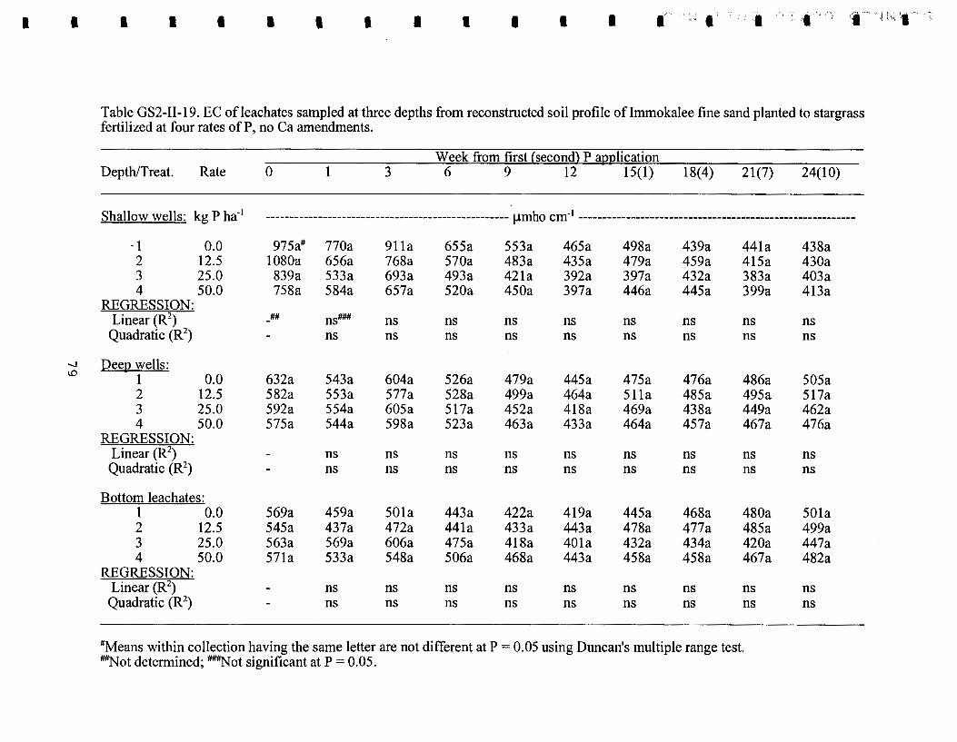
I I I I I I I I I I I I I I 'Lll-,;:·t ··f···) 'I. ;,!·)··
Table GS2-II-19. EC ofleachates sampled at three depths from reconstructed soil profile oflmmokalee fine sand planted to stargrass fertilized at four rates of P, no Ca amendments.
Week from first (second) P am2lication Depth/Treat. Rate 0 1 3 6 9 12 IS( I) 18(4) 21(7) 24(10)
Shallow wells: kg P ha·' --------------------------------------------------- ~mho em·' ----------------------------------------------------------
-1 0.0 97Sa# 770a 91la 6SSa SS3a 46Sa 498a 439a 441a 438a 2 12.5 1080a 6S6a 768a S70a 483a 43Sa 479a 4S9a 41Sa 430a 3 2S.O 839a 533a 693a 493a 421a 392a 397a 432a 383a 403a 4 SO.O 758a S84a 6S7a 520a 4SOa 397a 446a 44Sa 399a 413a
REGRESSION: Linear (R2
) -## ns### ns ns ns ns ns ns ns ns Quadratic (R2
) - ns ns ns ns ns ns ns ns ns
" DeeQ wells: \!)
1 0.0 632a 543a 604a S26a 479a 44Sa 475a 476a 486a SO Sa 2 12.S S82a SS3a S77a S28a 499a 464a Slla 48Sa 49Sa Sl7a 3 2S.O S92a 5S4a 60S a S17a 4S2a 418a 469a 438a 449a 462a 4 50.0 S7Sa S44a S98a S23a 463a 433a 464a 4S7a 467a 476a
REGRESSION: Linear (R2
) - ns ns ns ns ns ns ns ns ns Quadratic (R2
) - ns ns ns ns ns ns ns ns ns
Bottom leachates: 1 0.0 S69a 4S9a SOla 443a 422a 419a 44Sa 468a 480a SOla 2 12.S S4Sa 437a 472a 441a 433a 443a 478a 477a 48Sa 499a 3 2S.O S63a S69a 606a 47Sa 418a 401a 432a 434a 420a 447a 4 SO.O S71a S33a S48a S06a 468a 443a 4S8a 4S8a 467a 482a
REGRESSION: Linear (R2
) - ns ns ns ns ns ns ns ns ns Quadratic (R2
) - ns ns ns ns ns ns ns ns ns
#Means within collection having the same letter are not different at P = O.OS using Duncan's multiple range test. ~ot determined; ~ot significant at P = O.OS.

Table GS2-II-20. pH ofleachates sampled at three depths from reconstructed soil profile oflmmokalee fine sand planted to stargrass fertilized at four rates of P, no Ca amendments.
Week from first (second) P agglication Depth/Treat. Rate 0 1 3 6 9 12 15(1) 18(4) 21(7) 24(10)
Shallow wells: kg P ha-1 -------------------------------------------------------- pH ------------------------------------------------------------
1 0.0 7.04a# 6.70a 6.47a 6.86a 6.56a 6.34a 6.39a 6.23a 6.60a 6.32a 2 12.5 6.84a 6.78a 6.51a 6.69a 6.61a 6.23a 6.43a 6.31a 6.49a 6.28a 3 25.0 6.99a 6.81a 6.61a 6.80a 6.64a 6.23a 6.47a 6.41a 6.45a 6.36a 4 50.0 7.08a 6.84a 6.80a 6.85a 6.72a 6.29a 6.58a 6.39a 6.90a 6.47a
REGRESSION: Linear (R2
) -## nslff!# ns ns ns ns ns ns ns ns Quadratic (R2
) - ns ns ns ns ns ns ns ns ns
co Deeg wells: 0 1 0.0 7.45a 6.99a 7.03a 6.74a 6.43a 6.25a 6.23a 6.21a 6.14b 6.02a
2 12.5 7.32a 6.92a 7.07a 6.78a 6.42a 6.19a 6.34a 6.34a 6.23a 6.17a 3 25.0 7.11a 7.06a 7.25a 6.67a 6.31a 6.24a 6.49a 6.18a 6.22a 6.01a 4 50.0 7.41a 6.75a 6.81a 6.81a 6.41a 6.12a 6.34a 5.59a 6.16a 5.72a
REGRESSION: Linear (R2
) - ns ns ns ns ns ns 0.31 * ns ns Quadratic (R2
) - ns ns ns ns ns ns 0.32* ns ns
Bottom leachates: 1 0.0 6.12a 6.46a 6.10a 6.00a 5.67a 5.65a 5.83b 5.37a 5.25a 5.05a 2 12.5 6.16a 6.37a 6.14a 6.07a 5.81a 5.49a 6.05ab 5.61a 5.44a 5.43a 3 25.0 6.13a 6.09a 5.88a 5.82a 5.67a 5.67a 6.16a 5.37a 5.38a 5.35a 4 50.0 7.06a 6.40a 6.20a 6.15a 5.86a - 5.60a 6.15a 5.59a 5.54a 5.26a
REGRESSION: Linear (R2
) - ns ns ns ns ns 0.30* ns ns ns Quadratic (R2
) - ns ns ns ns ns 0.30* ns ns ns
#Means within collection having the same letter are not different at P = 0.05 using Duncan's multiple range test. ~ot determined; ~ot significant at P = 0.05; *Significant at P = 0.05.
I I I I I I • I I I I I I I I I • I I

I I I I I I I I I I I I I I --
- '") I --'!'I , ,_·I : ,.-- j :\i 't-
Table GS2-II-21. Phosphorus concentrations in leachates sampled at three depths from reconstructed soil profile oflmmokalee fine sand planted to stargrass fertilized at four rates of P, no Ca amendments.
Week from first (second) P annlication Depth/Treat. Rate 0 1 3 6 9 12 15(1) 18(4) 21(7) 24(10)
Shallow wells: kg P ha-1 ----------------------------------------------------- rng ~-I ----------------------------------------------------------
1 0.0 3.14a# 2.11a 1.71a l.Ola 1.09a 0.73b 0.56a 0.83a 0.8lb 0.84a 2 12.5 4.17a 3.05a 2.33a 1.84a 1.66a 1.36a 1.37a 1.32a 1.15ab 1.29a 3 25.0 3.75a 2.35a 2.20a 2.09a 1.69a 1.49a 0.79a 1.28a 1.30a 1.23a 4 50.0 2.90a 2.55a 2.08a 1.80a 1.72a 1.39a 1.34a 1.22a l.lOab 1.4la
REGRESSION: Linear (R2
) -## ns### ns ns ns ns ns ns ns ns Quadratic (R 2) - ns ns ns ns ns ns ns ns ns
CD Deen wells: ......
1 0.0 0.20a 0.18a 0.16a 0.20a 0.16a 0.14a 0.09a 0.13a 0.21a 0.22a 2 12.5 0.19b 0.16a 0.15a 0.14a 0.22a 0.14a 0.16a 0.15a 0.23a 0.14a 3 25.0 0.21a 0.18a 0.07a 0.18a 0.19a 0.22a O.lla 0.17a 0.18a 0.17a 4 50.0 0.17ab 0.17a 0.13a 0.14a 0.16a 0.09a 0.09a 0.15a 0.17a 0.13a
REGRESSION: ~inear (R2
) - ns ns ns ns ns ns ns ns ns Quadratic (R2
) - ns ns ns ns ns ns ns ns ns
Bottom leachates: 1 0.0 0.13a O.lOa O.lOa 0.13a 0.07a 0.07a 0.15a 0.16a 0.13a 0.15a 2 12.5 0.13a O.lOa 0.15a 0.08a 0.13a O.lla 0.14a 0.12a 0.12a 0.13a 3 25.0 0.16a 0.13a 0.12a 0.02a 0.10a 0.05a O.lla O.lla 0.12a 0.14a 4 50.0 0.17a O.lla 0.07a 0.04a 0.06a 0.08a 0.15a O.lla 0.15a 0.14a
REGRESSION: ~inear (R2
) - ns ns ns ns ns ns ns ns ns Quadratic (R2
) - ns ns ns ns ns ns ns ns ns
#Means within collection having the same letter are not different at P = 0.05 using Duncan's multiple range test. ~ot determined; ~ot significant at P = 0.05.

• Table GS2-II -22. Relationships between leachate P concentrations (Y) and EC (X) ofleachates from • reconstructed soil profile of Immokalee fine sand planted to stargrass fertilized twice at 0, 12.5, 25, and 50 kg P ha-1
, no Ca amendments.
Variable (range) Unit Regression equation No. of obs.# R2 Probability
Shallow wells: EC (400 to 1100) Y = 0.0037X- 0.3179 40 0.6177 2E-09
Deep wells: EC ( 400 to 650) Y = 6E-05X + 0.1327 40 0.0065 0.6203
Bottom leachates: EC (425 to 750) !J.mho cm-1
Y = 0.0002X + 0.0193 40 0.0804 0.0762
All depths: EC ( 400 to 11 00) Y = 0.0045X - 1.6285 120 0.3331 5E-12
#Each observation is the average of four replicates.
Cations and Pin leachates. The significant positive associations between Ca and Pin leachates at various depths (Table GS2-II-24) indicated that Ca was the primary cation that served as ion-pair with the various anionic P species such as H2P04-, HP04--, and P04 ___ that gave mobility toP in the whole soil profile even in the absence of Ca amendments.
The significant positive slope for Mg and Pin shallow wellleachates simply indicated the effect of Ca on Mg and on P in the Ap+E horizons. The more Cain the Ap+E leachates the more Mg and
•
•
•
--• •
•
-•
P were brought into or kept in solution (Table GS2-II-24). No significant associations between Mg • and P were noted in the deep wells due to the selective adsorption of P by the Bh horizon and the release of more Mg from the same horizon into the soil water. Both P and Mg appeared to have been similarly reduced as the Ap+E+Bh leachates crossed the C horizon thus keeping Mg and P • concentration ratios unchanged.
The associations between P and Kin leachates were very similar to those ofCa (Table GS2-II- • 24 ). Like Ca, K was strongly retained in the Bh horizon (deep wells). Unlike Ca, K was not retained in the C horizon (bottom leachates).
Phosphorus was significantly and positively associated withAl in shallow and deep wells and in bottom leachates (Table GS2-II-24). Because Al concentrations in leachates were extremely low,
• the slopes were relatively high. The significant positive slope in the deep wellleachates, unlike the a slopes for EC, Ca, Mg, or K, which were not significant or tended to be negative, would indicate that
82 •
•
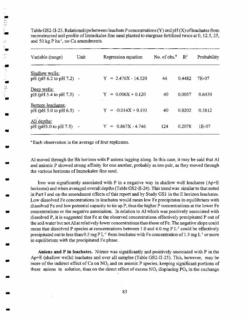
~~
-•
-•
-.. •
---
Table GS2-II-23. Relationships between leachate P concentrations (Y) and pH (X) ofleachates from reconstructed soil profile oflmmokalee fine sand planted to stargrass fertilized twice at 0, 12.5, 25, and 50 kg P ha-1
, no Ca amendments.
Al moved through the Bh horizon with P anions tugging along. In this case, it may be said that Al and anionic P showed strong affinity for one another, probably as ion-pair, as they moved through the various horizons oflmmokalee fine sand .
Iron was significantly assoc.iated with Pin a negative way in shallow wellleachates (Ap+E horizons) and when averaged overall depths (TabJe GS2-II-24). This trend was similar to that noted in Part I and on the amendment effects ofthis report and by Study GS1 in theE horizon leachates. Low dissolved Fe concentrations in leachates would mean low Fe precipitates in equilibrium with dissolved Fe and low potential capacity to tie up P, thus the higher P concentrations at the lower Fe concentrations or the negative association. In relation to Al which was positively associated with dissolved P, it is suggested that Fe at the observed concentrations effectively precipitated Pout of the soil water but not AI at relatively lower concentrations than those ofF e. The negative slope could mean that dissolved P species at concentrations between 1.0 and 4.0 mg P L-1 could be effectively precipitated out to less than 0.5 mg P L- 1 from leachates with Fe concentration of 1.5 mg L-1 or more in equilibrium with the precipitated Fe phase .
Anions and P in leachates. Nitrate was significantly and positively associated with P in the Ap+E (shallow wells) leachates and over all samples (Table GS2-II-25). This, however, may be more of the indirect effect of Ca on N03 and on anionic P species, keeping significant portions of these anions in solution, than on the direct effect of excess N03 displacing P04 in the exchange
83

-Table GS2-II-24. Relationships between leachate P concentrations (Y) and cations (X) in leachates -from reconstructed soil profile oflmmokalee fine sand planted to stargrass fertilized twice at 0, 12.5, 25, and 50 kg P ha-1, no Ca amendments.
• Variable (range) Unit Regression equation No. ofobs.# R2 Probability
• Shallow wells: Ca (20 to 200) mgL-1 Y = 0.022X - 0.098 44 0.8038 2E-16 -Mg (4 to 33) II Y = 0.126X - 0.386 44 0.3885 6E-06 K (30 to 80) II Y = 0.048X - 0.331 44 0.5707 3E-09 AI (0.2 to 0.75) II Y = 5.714X - 0.763 44 0.6314 1E-10 • Fe.(0.1 to 1.4) II Y = -2.577X + 2.517 44 0.2440 0.0007 -Dee~ wells: Ca (35 to 80) mgL-1 Y = 0.001X + 0.084 40 0.1413 0.0168 Mg (20 to 60) II Y = -0.001X + 0.179 40 0.0133 0.4786 • K (22.5 to 34) II Y = -0.002X + 0.222 40 0.0073 0.5990 AI (0.2 to 1.3) II Y = 0.101X + 0.120 40 0.0910 0.0585 Fe (0.07 to 1.0) II Y = -0.023X + 0.168 40 0.0106 0.5276 • Bottom leachates: Ca (18 to 50) mgL-1 Y = 0.002X + 0.031 40 0.2027 0.0036 • Mg (20 to 50) II Y = 6E-05X + 0.111 40 0.0002 0.9383 K (22 to 37) II Y = 0.005X - 0.018 32 0.1820 0.0149 AI (0.1 to 1.3) II Y= 0.004X + 0.112 40 0.0008 0.8637 • Fe (0.02 to 4.5) II Y= 0.001X + 0.119 32 0.0015 0.8308
• · All dsmths: Ca (20 to 200) mgL-1 Y= 0.027X - 0.853 124 0.8187 5E-47 Mg (4 to 60) II Y= -0.051X + 2.122 124 0.2760 4E-10 • K (22.5 to 80) II Y= 0.072X 1.733 116 0.7455 1E-35 -AI (0.1 to 1.3) II Y= 0.626X + 0.443 124 0.0156 0.1672 Fe (0.01 to 4.5) II Y=-0.375X + 1.015 116 0.1051 0.0004 -#Each observation is the average of four replicates. •
•
-84 -
•

< •
,. .
•
•
•
•
-•
-•
--•
•
•
-
Table GS2-II-25. Relationships between leachate P concentrations (Y) and anions (X) in leachates from reconstructed soil profile oflmmokalee fine sand planted to stargrass fertilized twice at 0, 12.5, 25, and 50 kg P ha-1
, no Ca amendments.
Variable (range) Unit Regression equation No. of obs.# R2 Probability
Shallow wells: N03 (0 to 55) mgL-1 Y= 0.047X + 1.230 44 0.7708 5E-15 S04 (1 oo to 400) " Y= 0.011X - 0.783 44 0.2961 0.0001 Cl (9 to 27) " Y= 0.059X + 0.788 44 0.0357 0.2195
Deen wells: N03 (0 to 9) mgL-1 Y = 0.0040X + 0.1570 40 0.0368 0.2354 S04 (130 to 275) " Y = -0.0003X + 0.2209 40 0.0195 0.3900 C) (20 to 47) " Y = 0.0009X + 0.1350 40 0.0213 0.3685
Bottom leachates: N03 (0) mgL-1
S04 (11 o to 340) " Y= 0.0004X - 0.0231 40 0.1344 0.0200 Cl (20 to 55) " Y= 0.0005X + 0.0973 40 0.0104 0.5303
All denths: N03 (0 to 55) mgL-1 Y = 0.065X + 0.570 84 0.6737 1E-21 S04 (100 to 400) " Y = 0.006X - 0.560 124 0.0377 0.0308 Cl (9 to 55) " Y = -0.071X + 2.537 124 0.3566 2E-15
#Each observation is the average of four replicates .
complex. Again, no matter how remote, it could also mean that the high N03 concentrations kept proportionate amounts of anionic P in solution. The reduction in N03 concentrations in deep well leachates would indicate that this anion was relatively strongly adsorbed by the Bh horizon or that the roots were able to effectively utilize the nitrates for plant growth.
Sulfate and P concentrations were positively and significantly associated in the Ap+E (shallow wells) and in Ap+E+Bh+C (bottom) leachates but tended to be negatively associated in Ap+E+Bh (deep well) leachates (Table GS2-II-25). Again, the positive and significant association could be more ofthe indirect effect ofCa on S04 and on anionic P species, keeping significant portions of them in solution, than on the direct effect of excess so4 displacing anionic p species from the exchange complex. But because of the divalence of the sulfate there is greater probability for S04
than for N03 doing just that and also, by competing with anionic P for adsorption sites, keeping
85

-significant amounts of fertilizer P from being adsorbed unto the exchange complex ofthe soil solids. @lilt
The slope for the deep wellleachates, which tended to be negative, would indicate that the anionic P species were preferentially retained in the Bh horizon over the S04 anions.
Chloride was not significantly associated with P at all depths indicating poor ability of Cl to replace Pin the exchange complex (Table GS2-II-25). The Bh horizon appeared to have augmented
•
Cl concentration ofthe Ap+E+Bh while the C horizon appeared to have no retention capacity for Cl. •
Effects of Calcium Amendments on Stargrass Forage Yield and Quality
This section presents the effects of the various Ca amendments on forage yield and quality of stargrass grown on reconstructed soil profile of Immokalee fine sand all fertilized at 50 kg P ha-1
•
Forage yield and percent dry matter. The various Ca amendments showed no effects on dry matter content of the forage or on forage dry matter yield. However, gypsum at 2 and 4 and dolomite at 4 Mg ha-1 tended to have higher yields than the control (TableGS2-II-26).
Phosphorus and other macro nutrients in forage. Limestone at 2 and 4 Mg ha-1 reduced P uptake by stargrass (Table GS2-II-26). This would indicate that despite the grinding of the material into powder, the effectiveness of limestone to render Pless mobile hence less available to plant, due most probably to precipitation unto the surfaces of the particles, remained operative. Gypsum at 2 and 4 Mg ha-1 also tended to reduce P uptake. This could be due to the fast leaching of Ca from gypsum with Ca dragging the P04 into deeper horizons beyond the reach of the just-establishing plant roots during the early stage of growth.
Calcium in gypsum-treated pots, which were already very high in the control, appeared to have augmented Ca uptake but not in limestone- or dolomite-treated pots. This would indicate that Cain these liming materials remained less available for plant use despite grinding them into powder.
Potassium uptake appeared to have been enhanced by gypsum but not by the liming materials. This tendency had been observed by the authors also in their phospho gypsum studies (Rechcigl et
•
•
•
•
•
•
•
• al., 1996). •
Magnesium uptake tended to increase in gypsum-amended soils contrary to the just above-cited study with phosphogypsum which showed adverse effects of gypsum on Mg uptake, especially during the first year of gypsum application. This could be due to the presence of a steady source of Mg in the soil.
Micro nutrients in forage. All the Ca amendments showed no effects on AI or Fe uptake although AI in forage tended to be higher in amended plants than in the control plants, and even linearly increased with rates in the case of dolomite (Table GS2-II-26). Copper and Zn uptakes differed only between gypsum at 4 and limestone at 2 Mg ha-1 rates, while Mn uptake was significantly adversely affected by limestone· and tended to be so adversely affected by dolomite. Gypsum, on the other hand, tended to increase Mn uptake.
86
•
•
•
•
•

I I I I • I I • I I I I I I I I -. iT I ) 'I----.. ; \'j ·a-
Table GS2-II -26. Total dry matter yield (DMY), percent dry matter (%DM), and total elemental uptake by stargrass planted in reconstructed soil profile oflmmokalee fine sand fertilized at 50 kg P ha-1 applied twice and amended with Ca amendments.
Amendment Rate %DM DMY p K Ca Mg Fe AI Cu Zn Mn
Mg ha-1 % g por1
-------------------------------------- mg pof I -------------------------------------------
No amendment 0 25.6a# 46.5ab 138a 404bc 304bc 131ab 3.15a 314a 0.61ab 1.82ab 1.39ab
Gypsum 2 27.0a 51.7ab 124ab 479ab 359ab 131ab 3.43a 470a 0.68ab 1.78ab 1.55a 4 26.1a 53.1a 122ab 539a 380a 137ab 3.25a 379a 0.81a 1.94a 1.53a
Limestone 2 24.7a 40.8b 90c 356c 250c 93a 2.91a 339a 0.52b 1.37b 0.93c 4 26.9a 43.0ab lOObc 397bc 301bc llObc 3.23a 421a 0.68ab 1.65ab 1.04c
co -...)
Dolomite 2 24.1a 44.8ab 124ab 373c 263c 124ab 2.99a 404a 0.73ab 1.71ab 1.08bc 4 27.3a 52.5a 139a 42lbc 338ab 150a 3.95a 526a 0.64ab 1.94a 1.14bc
REGRESSION: Mined Gy:nsum
Linear (R2) ns## ns ns 0.47'' 0.35* ns ns ns 0.37* ns ns
Quadratic (R2) ns ns ns 0.49" 0.35* ns ns ns 0.38* ns ns
Ca carbonate Linear (R2
) ns ns 0.47* ns ns ns ns ns ns ns 0.44* Quadratic (R 2) ns ns 0.44* ns ns ns ns ns ns ns 0.40"
Dolomite Linear (R2
) ns ns ns ns ns ns ns 0.47" ns ns 0.42" Quadratic (R2
) ns ns ns ns ns ns ns 0.40" ns ns 0.41*
#Means within columns having the same letter are not different at P .::S 0.05 based on Duncan's multiple range test. ## ns =not significant; • Significant at.:::::; 0.05.

-Effects of Phosphorus Fertilizer on Stargrass Forage Yield and Quality
The results presented in this section were obtained from pots fertilized at four rates ofP with no Ca amendments. •
Forage yield and percent dry matter. Table GS2-II-27 shows that P fertilizer applied twice at 12.5, 25.0 and 50 kg P ha-1 to stargrass grown on reconstructed soil profile oflmmokalee fine sand • had no beneficial effects on forage dry matter yield or on dry matter content. This strongly indicated that P was readily available in sufficient amounts in these soils for optimum stargrass needs.
Phosphorus and other macro nutrients in forage. Fertilizer P increased P contents in forage from 0.20 to 0.30% asP rates increased from 0 to 50 kg P ha-1 (Table GS2-II-27) but not forage yield as noted earlier. Thus, stargrass having P contents within the range would not benefit from P fertilization in terms of forage yield. Similar observations were noted earlier in the individual soil horizons study (GS2-I). Fertilizer P had no effects on Ca, K, or Mg contents in forage (Table GS2-II-27). A Ca:P ratio of 3.1:1 for the control and 2.2:1 for the highest for P fertilizer rate were well within the desirable Ca:P ratio range of not less than 1:1 to not more than 7:1 (Wise et al., 1963).
Micro nutrients in forage. The various Prates also had no effects on Fe, Cu, Mn, Zn, and AI. Iron and AI, however, tended to increase with rates while the concentrations of the other micro
•
...
•
•
nutrients remained relatively similar (Table GS2-II-27). •
Effects of Calcium Amendments on Soil
At the end ofthe study, representative samples from Ap, E, and Bh horizons ofthe reconstructed soil profile of Immokalee fine sand were obtained for the various analyses.
Ap horizon. Relative to the control, all Ca amendments had no effects on soil pH (Table GS2-II-28). Between theCa amendments, gypsum at 4 Mg ha-1 showed lower pH than limestone at 2 but not at 4 Mg ha-1
• All Ca-amended soils tended to have lower extractable P than the control indicating possible reduced extractability of soil P. Limestone and dolomite at 4 Mg ha-1 tended to have the least Mehlich-extractable P. All Ca amendments had no effects on K, Ca, Mg, and Fe in the Ap horizon.
E horizon. Relative to the control no effects of the various Ca amendments were noted on E soil pH (Table GS2-II-29). Limestone at 2 but not at 4 Mg ha-1 indicated a higher soil pH than gypsum at 2 but not at 4 Mg ha-1
• Although not significantly different from any other treatment, limestone at 4 Mg ha-1 showed the lowest extractable P. No other effects of theCa amendments were noted.
Bh horizon. Relative to the control no effects of the various Ca amendments on soil P or other soil variables were noted in the Bh horizon soils (Table GS2-II-30). Dolomite at 4 Mg ha-1 showed higher soil pH than gypsum also at 4 Mg ha-1 but not over the control. Limestone at 2 Mg ha-1
showed higher K than gypsum at 4 Mg ha-1 but not over the control.
88
•
•
•
• .. •
-•
-•

I I
co 1.0
I I I a I • I I I ...
•• ••• i •... .• -- ,, ('.; ., . I I I '·' I
Table GS2-II-2 7. Total dry matter yield (DMY), percent dry matter (%D M), and total elemental uptake by star grass planted in reconstructed soil profile of Immokalee fine sand fertilized at four rates of P applied twice, no Ca amendments.
Treatment Rate %DM DMY p K Ca Mg Fe AI Cu Zn Mn
kg ha- 1 % gpor1 -------------------------------------- mg por 1
-------------------------------------------
1 0.0 25.6a# 45.5a 89b 380a 276a 115a 2.85a 294a 0.75a 1.78a 1.37a 2 12.5 27.0a 47.5a 103b 394a 296a 141a 3.05a 311a 0.86a 1.85a 1.43a 3 25.0 26.la 45.4a 104b 365a 272a 12la 3.28a 454a 0.78a 1.77a 1.36a 4 50.0 24.7a 46.5a 138a 404a 304a 131a 3.15a 314a 0.6la 1.82a 1.39a
REGRESSION: Linear (R2
) ns## ns 0.64* ns ns ns ns ns ns ns ns Quadratic (R2
) ns ns 0.63* ns ns ns ns ns ns ns ns
#Means within columns having the same letter are not different at P :S 0.05 based on Duncan's multiple range test. ## ns =not significant; * Significant at :S 0.05.

-Table GS2-II-28. Soil pH and Mehlich I extractable elements in Ap horizon of reconstructed soil profile of Immokalee fme planted to stargrass fertilized twice at 50 kg ha·1
, with the second P -application applied 14 weeks after the first, and amended with Ca amendments.
Amendment Rate pH p K Ca Mg Fe •
Mgkg·1 k -1 --------------------- mg g ------------------------------- •
No amendment 0 5.9ab# 9.2a 5.9a 1423a 90.0a 7.6a •
Gypsum 2 5.9ab 6.2a 6.2a 1326a 77.0a 7.3a 4 5.7b 5.8a 5.3a 1214a 7l.Oa 6.2a
• Limestone 2 6.0a 5.8a 4.9a 1272a 77.0a 7.4a
4 5.9ab 5.6a S.la 1329a 66.0a 7.1a
• Dolomite 2 5.9ab 7.4a 6.la 1313a 77.0a 6.7a
4 5.9ab 5.6a 5.3a 1212a 76.0a 7.3a REGRESSION: • Mined Gx12sum
Linear (R2) 0.25* ns## ns ns ns ns
Quadratic (R2) 0.25* ns 147ns ns ns ns • Limestone
Linear (R2) ns 0.25* ns ns ns ns
Quadratic (R2) ns 0.29* ns ns ns ns • Dolomite
Linear (R2) ns ns ns ns ns ns
Quadratic (R2) ns ns ns ns ns ns •
# Means within columns having the same letter are not different at P .:S 0.05 based on Duncan's • multiple range test. ## ns =not significant; * Significant at .:S 0.05. -
•
•
•
90 •
•

:• ·:: ...
~~
Table GS2-II-29. Soil pH and Mehlich I extractable elements in E horizon of reconstructed soil
• profile oflmmokalee fine with the Ap horizon planted to stargrass fertilized twice at 50 kg ha"1, with
the second P application applied 14 weeks after the first, and amended with Ca amendments.
:• Amendment Rate pH p K Ca Mg Fe
--·.:~ Mg kg-1 k -1 --------------------- mg g -------------------------------
•• No amendment 0 6.2ab 1.8a 1.8a 48a 4.0a 0.6a
• Gypsum 2 6.lb 1.9a 1.9a 41a 4.0a 0.4a 4 6.2ab 1.4a 2.1a 55 a 8.0a 0.4a
• Limestone 2 6.3a 1.6a 2.0a 43a 4.0a 0.5a 4 6.2ab l.la 2.9a 39a 4.0a 0.3a
• Dolomite .2 6.1b 1.9a 2.1a 37a 4.0a 0.9a 4 6.lb 1.9a 1.7a 45a 4.0a 0.5a
REGRESSION:
• Mined GyQsum Linear (R2
) ns ns ns ns ns ns Quadratic (R2
) ns ns ns ns ns ns • Limestone Linear (R2
) ns 0.34* ns 0.37* ns ns Quadratic (R2
) ns 0.36* ns 0.38* ns ns - Dolomite Linear (R2
) ns ns ns ns ns ns - Quadratic (R2) ns ns ns ns ns ns
- # Means within columns having the same letter are not different at P _:::: 0.05 based on Duncan's multiple range test. ## ns = not significant; * Significant at_:::: 0.05. -..
-- 91
-

Table GS2-II-30. Soil pH and Mehlich I extractable elements in Bh horizon of reconstructed soil profile oflmmokalee fine with the Ap horizon planted to stargrass fertilized twice at 50 kg ha-1
, with the second P application applied 14 weeks after the first, and amended with Ca amendments.
Amendment Rate pH p K Ca Mg Fe
Mg kg-1 k -1 --------------------- mg g -------------------------------
No amendment 0 5.5ab 133.1a 37.7ab 962a 141a 6.6a
Gypsum 2 5.6ab 150.4a 33.4ab 897a 107a 7.2a 4 5.4b 119.3a 32.9a 836a 118a 7.2a
Limestone 2 5.6ab 107.2a 40.8b 1130a 143a 7.6a 4 5.5ab 128.8a 35.1ab 903a 113a 6.5a
Dolomite 2 5.7a 152.3a 34.1ab 968a 144a 6.7a 4 5.6ab 127.9a 37.3ab 1010a 141a 7.0a
REGRESSION: Mined Gy~sum
Linear (R2) ns ns ns ns ns ns
Quadratic (R2) ns ns ns ns ns ns
Limestone Linear (R2
) ns ns ns ns ns ns Quadratic (R2
) ns ns ns ns ns ns Dolomite
Linear (R2) ns ns ns ns ns ns
Quadratic (R2) ns ns ns ns ns ns
#Means within columns having the same letter are not different at P,::::: 0.05 based on Duncan's multiple range test. ## ns = not significant.
Effects of Phosphorus Fertilizer on Soil
Ap horizon. Table GS2-II-31 shows that P fertilizers up to 100 kg ha-1 to a reconstructed soil profile oflmmokalee fine sand planted to stargrass had no effects on soil pH or on the concentrations of K, Ca, Mg, or Fe. The highest Prate, however, increased extractable P in Ap over the lower P fertilizer rates including the control which had the lowest soil P.
92
-.. -•
-•
•
•
•
•
•
--•
•
• .. •

,. .. • 1'•,
-•
•
-•
•
•
--•
•
•
•
•
•
Table GS2-II-31. Soil pH and Mehlich I extractable elements in Ap horizon of reconstructed soil profile of Immokalee fine planted to stargrass fertilized twice at four rates of P, with the second P application applied 14 weeks after the first, no Ca amendments .
Treatment Rate pH p K Ca Mg Fe
kg P ha·1 k .) ----------------------- mg g -------------------------------
1 0.0 5.9a# 4.6b 5.3a 1222a 78.0a 6.4a 2 12.5 5.9a 4.9b 5.4a 1249a 77.0a 5.9a 3 25.0 5.9a 5.2b 5.0a 1279a 65.0a 7.la 4 50.0 5.9a 9.2a 5.9a 1423a 90.0a 7.6a
REGRESSION: Linear (R2
) ns## ns ns ns ns ns Quadratic (R2
) ns ns ns ns ns ns
#Means within columns having the same letter are not different at P::;: 0.05 based on Duncan's multiple range test. ## ns = not significant .
E horizon. Phosphorus fertilizers reduced the pH of theE horizon when compared to that of the control (Table GS2-II-32). No other effects ofP fertilizers applied to the surface of the Ap were noted in the E horizon .
Bh horizon. No effects of fertilizer P applied up to 100 kg ha-1 to the surface of the Ap horizon of reconstructed soil profile of Immokalee fme sand planted to stargrass were noted in the Bh horizon (Table GS2-II-33).
Accounting for Soil and Fertilizer Phosphorus in Ca-amended Soil
The summary for Pin plant tissue (with the exception of the roots and the stubble portions), in leachate withdrawn for analysis, and in soil is given in Table GS2-II-34. Total Pin leachates was the sum of the products of the volumes and the corresponding concentrations for ten samplings done during the period of study .
The Pin above-ground plant tissue represented only from 7 to 9 percent of the post-study total P accounted for (Table GS2-II-34). Subtracting 89 mg P por1 extracted by the plants in the no P and no amendment treatments (Table GS2-II-26), stargrass plants utilized only 15.1, 10.8, 0.3, and 10.8 %of the 100 kg ha-1 fertilizer Pin no amendment, gypsum-, limestone-, and dolomite-amended pots, respectively (Table GS2-II-34). This and the fact that there were no effects of P rates on yield indicated that stargrass pasture on Immokalee fine sand would not benefit from P fertilization.
93

Table GS2-II-32. Soil pH and Mehlich I extractable elements in E horizon of reconstructed soil profile oflmmokalee fine sand with the Ap horizon planted to stargrass fertilized twice at four rates of P, with the second P application applied 14 weeks after the first, no Ca amendments.
Treatment Rate pH p K Ca Mg Fe
kg P ha·1 k -1 ----------------------- mg g -------------------------------
1 0.0 6.5a 1.5a 1.8a 50a 4.0a 0.4a 2 12.5 6.3b 1.3a 1.6a 39a 4.0a 0.4a 3 25.0 6.3b 1.8a 1.7a 48a 4.0a 0.6a 4 50.0 6.1b 1.8a 1.8a 48a 4.0a 0.6a
REGRESSION: Linear (R2
) 0.39* ns ns ns ns ns Quadratic (R2
) 0.39* ns ns ns ns ns
#Means within columns having the same letter are not different at P.:::;: 0.05 based on Duncan's multiple range test. ## ns =not significant; * Significant at.:::;: 0.05.
Table GS2-II-33. Soil pH and Mehlich I extractable elements in Bh horizon of reconstructed soil profile of Immokalee fine With the Ap horizon planted to stargrass fertilized twice at four rates of
--•
•
•
-•
•
•
• P, with the second P application applied 14 weeks after the first, no Ca amendments. •
Treatment Rate pH p K Ca Mg Fe •
kg P ha·1 ----------------------- mg kg-1------------------------------- -
1 0.0 5.4a 143a 37.1a 791a 129a 6.5a 2 12.5 5.6a 146a 34.8a 839a 123a 7.0a
.. 3 25.0 5.5a 132a 36.6a 950a 114a 7.1a 4 50.0 5.5a 133a 37.7a 962a 141a 6.6a • REGRESSION:
Linear (R2) ns ns ns ns ns ns
Quadratic (R2) ns ns ns ns ns ns ..
# Means within columns having the same letter are not different at P .:::;: 0.05 based on Duncan's • multiple range test.
•

··~
:.
... -••
•
•
-•
•
•
-•
Table GS2-II-34. Accounting for soil and fertilizer Pin reconstructed soil profile oflmmokalee fine sand planted to stargrass fertilized twice at 50 kg P ha·I, with second P application applied 14 weeks after the first, and amended with Ca amendments at 2 Mg ha·I.
Treatment P Source No amendment Gypsum Limestone Dolomite
Fertilizer P +initial soil P: ------------------------Total mg P pori (%) ----------------------------
Fertilizer P a~Qlied 314.0 (21.9) 314.0 (21.9) 314.0 (21.9} 314.0 (21.9} P in soil column 1106.9 (77.3) 1106.9 (77.3) 1106.9 (77.3) 1106.9 (77.3) Ap 8.16 kg 115.9 (10.5) 115.9 (10.5) 115.9 (10.5) 115.9 (10.5) E 18.84 kg 22.6 ( 2.0) 22.6 ( 2.0) 22.6 ( 2.0) 22.6 ( 2.0) Bh 9.42 kg 968.4 (87.5) 968.4 (87.5) 968.4 (87.5) 968.4 (87.5) c# 2.35 kg
Sod' soil## 11.3 ( 0.8) 11.3 ( 0.8) 11.3 ( 0.8) 11.3 ( 0.8) Initial-Total 1432.2 (100} 1432.2 (100) 1432.2 (100) 1432.2 (100)
Post fertilization P sources: ------------------------Total mg P pori (%) ----------------------------
Plant tissue 138.00 (9.1) 124.00 (7.6) 90.00 (7.6) 124.00 (7.4) Leachate withdrawn i.71 (0.1) 1.79 (0.1) 2.13 (0.2} 1.65 (0.1)
Shallow wells 1.52 1.56 1.93 1.45 Deep wells 0.11 0.15 0.12 0.11 Bottom leachates 0.08 0.08 0.08 0.09
Soil column 1362.8 (90.0) 1503.2 (91.6) 1087.3 (91.3) 1530.9 (91.8) Ap 8.16 kg 75.1 ( 5.5) 50.6 ( 3.4) 47.3 ( 4.4) 60.4 ( 3.9) E 18.84 kg 33.9 ( 2.5) 35.8 ( 2.4) 30.2 ( 2.8) 35.8 ( 2.4) Bh 9.42 kg 1253.8 (92.0) 1416.8 (94.2) 1009.8 (92.8) 1434.7 (93.7) c# 2.35 kg
Sod soil## 11.3 (0.7) 11.3 (0.7) 11.3 (0.9) 11.3 (0.7) Post-Total 1513.8 (100) 1640.3 (1 00) 1190.7 (100.) 1667.9 (100)
---------------------------- post-P :pre-P ratio ----------------------------
Soil: ~ost-P:~re-P ratio 1.36 0.98 1.38
Total: ~ost-P:Qre-P ratio 1.14 0.83 1.17
#No analysis was done before and after the study. • ~ alues were those after the study using a sod soil of 500 g at 1.0 g cm·3 averaged over the two Ap
soils (Tables GS2-I-16 and GS2-I-17); no analysis of soil in sod was done prior to planting and P fertilization. ##lltJsing the value for Ap from Table GS1-3. -
• 95
•

In the soil profile, Mehlich-extractable P in the Ap horizon was reduced after the study in all treatments but increased in the Bh horizon with the least increase noted in limestone-treated pots (Table GS2-II-34). Total extractable P for the whole soil column or profile increased in the control (no amendment) and in gypsum- and dolomite-amended pots but not in limestone-amended ones as indicated by the post-P :pre-P ratios. This would indicate that the P retained in limestone-treated soils were not readily extracted by Mehlich I compared to those in pots that received other treatments. This was also noted in greenhouse study GS 1, a leaching study using individual soil horizons with no stargrass planted. Thus, the two greenhouse studies demonstrated the immobilizing effects of calcium carbonate on soil and fertilizer P.
Accounting for Soil and Fertilizer Phosphorus in Soil with No Ca Amendments
The summary for Pin plant tissue (with the exception of the roots and the stubble portions), in leachate withdrawn for analysis, and in soil fertilized at four rates of P with no Ca amendments is given in Table GS2-II-35. Total Pin leachates was the sum of the products of the volumes and the corresponding concentrations for ten samplings done during the period of study.
The Pin above-ground plant tissue represented only from 6 to 9 percent of the post-study total P accounted for. Subtracting 89 mg P por1 extracted by the plants in the no P and no amendment treatments (Table GS2-II-27), stargrass plants utilized only 17.3, 9.3, and 15.0% of fertilizer P applied at 25, 50, and 100 kg P ha·1
, respectively (Table GS2-II-35). This and the fact that there was no effects ofP rates on yield indicated strongly that stargrass pasture on Immokalee fine sand would not benefit from P fertilization.
In the soil profile, Mehlich-extractable P in the Ap horizon was also reduced after the study in all treatments but increased in the Bh horizon in similar magnitudes (Table GS2-II-35) for the four Prates. Total extractable P for the whole soil column or profile increased in the control (no P) and in P-fertilized pots as indicated by the total post-P:pre-P ratios but in decreasing ratios with increasing Prates. This would indicate that the non'-readily extractable P increases, mostly in the Bh
· horizon, with increasing Prates. This was also noted by Alcordo et al. (2002) in their leaching study using similar soil but no stargrass planted.
96
-.. -•
•
•
• •
•
•
•
--.. -•
•
•

l ...
··~
)I!!
..
.,
••
•
-•
.. •
--•
.. •
•
•
•
Table GS2-II-3 5. Accounting for soil and fertilizer P in reconstructed soil profile oflmmokalee fine sand planted to stargrass fertilized twice at four rates ofP, with the second P application applied 14 weeks after the first, no Ca amendments.
kg P ha·1
P Source NoP 12.5 25.0 50.0
Fertilizer P +initial soil P: ------------------------ Total mg P por 1 (%) ----------------------------
Fertilizer P am:1lied 0.0 ( 0.0) 78.5 ( 6.6) 157.0 (12.3) 314.0 (21.9) P in soil column 1106.9 (76.7) 1106.9 (76. 7) 1106.9 (76. 7) 1106.9 (76. 7) Ap 8.16 kg 115.9 ( 8.0) 115.9 ( 8.0) 115.9 ( 8.0) 115.9 ( 8.0) E 18.84 kg 22.6 ( 1.6) 22.6 ( 1.6) 22.6 ( 1.6) 22.6 ( 1.6) Bh 9.42 kg 968.4 (67.1) 968.4 (67.1) 968.4 (67.1) 968.4 (67.1) c# 2.35 kg
Sod soil## 11.3 ( 0.8) 11.3 ( 0.8) 11.3 ( 0.8) 11.3 ( 0.8) Initial-Total 1118.2 (100) 1196.7 (100) 1275.2 (100) 1432.2 (1 00)
Post fertilization P sources: ------------------------ Total mg P pot" 1 (%) ----------------------------
Plant tissue 89.0 (5.9) 103.00 (6.6) 104.0 (7.2) 138.00 (0.9) Leachate withdrawn 1.71 (0.1) 1.79 (0.1) 2.13 (0.1) 1.65
Shallow wells 1.14 1.73 1.68 1.52 Deep wells 0.13 0.13 0.13 0.11 Bottom leachates 0.09 0.08 0.08 0.08
Soil column 1412.9 (93.3) 1439.8 (92.5) 1319.7 (91.8) 1361.9 (90.0) Ap 8.16 kg 37.5 ( 2.7) 40.0 ( 2.8) 42.4 ( 3.2) 75.1 ( 5.5) E 18.84 kg 28.3 ( 2.0) 24.5 ( 1.7) 33.9 ( 2.6) 33.9 ( 2.5) Bh 9.42 kg 1347.1 (95.3) 1375.3 (95.5) 1243.4 (94.2) 1252.9 (92.0) c# 2.35 kg
Sod soil## 11.3 {0. 7) 11.3 (0.7) 11.3 {0.8) 11.3 {0.7) Post-Total 1514.0 (100) 1555.9 (100) 1437.1 (100.) 1512.9 (100)
---------------------------- post-P :pre-P ratio ----------------------------
Soil: post-P:pre-P ratio 1.28### 1.30 1.19 1.23
Total: post-P:nre-P ratio 1.35### 1.30 1.13 1.06
#No analysis was done before and after the study. ##Values were those after the study using a sod soil of 500 gat 1.0 g cm·3 averaged over the two Ap soils (Tables GS2-I-16 and GS2-I-17); no analysis of soil in sod was done prior to planting and p fertilization. ###Using the value for Ap from Table GS1-3.
97

Field Study 1 (AGFS): Stargrass P Fertilization Experiment
Effects on Forage Yield and Quality
Forage Yield and Percent Dry Matter (% DM)
Effects of fertilizer P. The effects of all 8 treatments are given in Table AGFS-3 for % DM and total DM forage yields. Phosphorus fertilization of stargrass pasture on Immokalee fine sand up to 50 kg P ha·1 showed no beneficial effects on forage yield or dry matter content in 1999, 2000, 2001, or when averaged over the three-year period. Table AGFS-4, which analyzed the effects of fertilizer P rates only, also indicated no effects of P fertilization on stargrass nor any significant trends in forage yield with P rates. No differences in % DM with treatments were noted. The greenhouse study conducted concurrently with the field study using similar treatments also showed no effects of fertilizer P on forage yield of stargrass grown on potted reconstructed soil profile of Immokalee fine sand (Rechcigl et al., 2002).
Effects of lime. Table AGFS-3 showed that calcium carbonate at 4 Mg ha·1 (T6), but not at 2 Mg (T5), applied to plots that received 50 kg P ha·1 tended to increase forage yield in 1999, 2000, and 2001, and when averaged overall. But the differences between T6 and T4 (50 P, no lime) or between T6 and T1 (0 P, no lime) were not significant. Table AGFS-5, for the lime treatments only, although showing no significant differences between rates or any significant trends in forage yield with rates, tended to have consistently higher forage yield at 4 Mg ha· 1 than at the lower rates. This would indicate that 4 Mg lime ha· 1
, or possibly higher, can be used as soil amendment to tie up P (Alcordo et al., 2002) without adverse effects on forage yield of stargrass. The greenhouse study using reconstructed soil profile of Immokalee fine sand, dolomite at 4 Mg ha·1 also showed similar tendency to increase stargrass forage yield (Rechcigl et al., 2002). No differences in% DM with treatments were noted.
Effects of gypsum. There was a tendency for 2 and 4 Mg gypsum ha· 1 to increase forage yield during the first year of application (1999) but not thereafter or when averaged over the three-year period (Tables AGFS-3 and AGFS-6). The one-year greenhouse study using reconstructed soil profile showed that gypsum at the said rates also tended to increase stargrass forage yield (Rechcigl et al., 2002). No differences in % DM with treatments were noted in both studies. However, since gypsum at the lower rate has been shown in a leaching study (Alcordo et al. 2002) to increase the mobility of soil or fertilizer Pin matrix flow, it should not be recommended as a soil amendment, as some studies did suggest (Anderson et al., 1995), to tie up P in Spodosols.
Crude Protein (CP) and in vitro Organic Matter Digestibility (IVOMD)
The value of a forage as a source of amino acids is reflected on the amount of total N contents. Forages contain N in many forms other than amino acids which may be converted to amino acid by rumen micrqorganisms. All forms ofN present in plants are included in the term crude protein (CP) which is obtained by multiplying total% N by 6.25. Protein contains 22 different amino acids and is necessary for the overall health and development of animal life.
98
•
•
•
-•
•
•
•
•
-•
--•
-•
•
..

il!ll ,.. ... •.. ,_,
, ... Table AGFS-3. Effects ofP fertilizer, calcium carbonate, and mined gypsum on percent dry matter (%DM) and total forage DM yield of stargrass pasture on Immokalee fine sand fertilized annually with P without or with Ca amendment applied once in 1999; 1999 (7 harvests), 2000 (6 harvests),
..... and 2001 (6 harvests) seasons .
• Year/Treatment p CaC03 Gypsum DM Forage yield
1999: kgha·1 ---------- Mg ha·1 --------- % MgDMha·1 - T1 0.00 0.0 0.0 38.0at 8.81b
T2 12.50 0.0 0.0 37.4a 8.29b
•• T3 25.00 0.0 0.0 33.8a 9.89ab T4 50.00 0.0 0.0 35.8a 9.97ab T5 50.00 2.0 0.0 35.2a 9.87ab T6 50.00 4.0 0.0 35.7a 10.88ab
• T7 50.00 0.0 2.0 33.6a 12.10a T8 50.00 0.0 4.0 34.la 11.93a 2000: T1 0.00 0.0 0.0 35.7a 9.28a • T2 12.50 0.0 0.0 36.la 7.34a T3 25.00 0.0 0.0 34.1a 7.63a T4 50.00 0.0 0.0 34.4a 8.44a
• T5 50.00 (2.0)tt 0.0 34.7a 8.42a T6 50.00 (4.0) 0.0 33.4a 9.53a T7 50.00 0.0 (2.0)tt 35.0a 8.44a T8 50.00 0.0 (4.0) 35.6a 8.05a
• 2001: T1 0.00 0.0 0.0 32.5a 11.88a T2 12.50 0.0 0.0 33.5a 11.12a - T3 25.00 0.0 0.0 32.la 12.90a T4 50.00 0.0 0.0 33.0a 11.87a T5 50.00 (2.0)tt 0.0 32.9a 11.80a T6 50.00 (4.0) 0.0 33.7a 12.18a .. T7. 50.00 0.0 (2.0)tt 33.5a 12.62a T8 50.00 0.0 (4.0) 34.2a 11.31a
- 3-year Mean: T1 0.00 0.0 0.0 35.5a 9.99a T2 12.50 0.0 0.0 35.8a 8.92a T3 25.00 0.0 0.0 33.4a 10.14a • T4 50.00 0.0 0.0 34.5a 10.09a T5 50.00 2.ott 0.0 34.3a 10.03a T6 50.00 4.0 0.0 34.3a 10.88a
• T7 50.00 0.0 2.ott 34.0a 11.05a T8 50.00 0.0 4.0 34.6a 10.43a
\ • t Means in column having the same letter are not different at the 5% level of significance using Tukey's Studentized Range (HSD) Test.
ttBased on initial rate of application made in 1999 .
•
- 99
•

• Table AGFS-4. Effects of P fertilizer applied annually without Ca amendments on percent dry • matter (%DM) and total forage DM yield of stargrass pasture on Immokalee fine sand; 1999 (7 harvests), 2000 (6 harvests), and 2001 (6 harvests) seasons.
• Year/Treatment p CaC03 Gypsum DM Forage yield
• 1999: kgha· 1 ---------- Mg ha-1
----------- % MgDMha-1
T1 0.0 0.0 0.0 38.oat 8.81a • T2 12.5 0.0 0.0 37.4a 8.29a T3 25.0 0.0 0.0 33.8a 9.89a T4 50.0 0.0 0.0 35.8a 9.97a Statistics: • P(treatment) 0.6099 0.2724 LSDo.os 6.6 2.02 P(linear) 0.4349 0.1286 • P( quadratic) 0.4059 0.9312 2000: n-- 0.0 0.0 0.0 35.7a 9.28a T2 12.5 0.0 0.0 36.1a 7.34a • T3 25.0 0.0 0.0 34.1a 7.63a T4 50.0 0.0 0.0 34.4a 8.44a Statistics: • P(treatment) 0.8836 0.3737 LSDo.os 5.8 2.3 P(linear) 0.5725 0.5537 P( quadratic) 0.8507 0.1388 • 2001: T1 0.0 0.0 0.0 32.5a 11.88a T2 12.5 0.0 0.0 33.5a 11.12a -T3 25.0 0.0 0.0 32.1a 12.90a T4 50.0 0.0 0.0 33.0a 11.87a Statistics: P( treatment) 0.9813 0.7784 • LSDo.os 7.2 3.40 P(linear) 0.9841 0.8217 P( quadratic) 0.9581 0.7304 -3-year mean: T1 0.0 0.0 0.0 35.5a 9.99a T2 12.5 0.0 0.0 35.8a 8.92a • T3 25.0 0.0 0.0 33.4a 10.14a T4 50.0 0.0 0.0 34.5a 10.09a Statistics: • P( treatment) 0.5747 0.4165 LSDoos 3.7 1.62 P(linear) 0.3994 0.6138 P( quadratic) 0.5929 0.6637 .. tMeans in column having the same letter are not different at P(treatment) ~ 0.05. •
100 •
•


• Table AGFS-6. Effects of mined gypsum on percent dry matter (%DM) and total forage DM yield • of stargrass pasture on Immokalee fine sand applied once in 1999 to plots fertilized annually at 50 kg P ha-1
; 1999 (7 harvests), 2000 (6 harvests), and 2001 (6 harvests) seasons.
• Treatment p CaC03 Gypsum DM Forage yield
• 1999: kgha- 1 ---------- Mg ha-1 ----------- % MgDMha- 1
T4 50.0 0.0 0.0 35.8at 9.97a • T7 50.0 0.0 2.0 33.6a 12.10a T8 50.0 0.0 4.0 34.1a 11.93a Statistics: P( treatment) 0.5381 0.2544 • LSDo.os 4.6 2.73 P(linear) 0.3210 0.1773 P( quadratic) 0.6171 0.3370 .. 2000: T4 50.0 0.0 0.0 34.4a 8.44a T7 50.0 0.0 (2.0)tt 35.0a 8.44a • T8 50.0 0.0 (4.0) 35.6a 8.05a Statistics: P(treatment) 0.9363 0.9292 • LSDo.os 6.1 2.29 P(linear) 0.7178 0.7409 P( quadratic) 0.9934 0.8487
• 2001: T4 50.0 0.0 0.0 33.0a 11.87a T7 50.0 0.0 (2.0)tt 33.5a 12.62a • T8 50.0 0.0 (4.0) 34.2a 11.31a Statistics: P(treatment) 0.9204 0.7352 LSDoos 6.1 3.35 • P(linear) 0.6857 0.7378 P( quadratic) 0.9761 0.4798
3-year mean: -T4 50.0 0.0 0.0 34.5a 10.09a T7 50.0 0.0 2.ott 34.0a 11.05a T8 50.0 0.0 4.0 34.6a 1 0.43a • Statistics: P(treatment) 0.9515 0.5168 LSDoos 3.2 1.67 • P(linear) 0.9298 0.7154 P( quadratic) 0.7624 0.2764
• t Means in column having the same letter are not different at P(treatment) _:s 0.05. ttBased on initial rate of application made in 1999.
• 102
•

; .. , ..
' ..... ·
••
-•
In vitro organic matter digestibility (IVOMD) is another measure of forage quality. The apparent digestibility of forage is the proportional difference between the quantities consumed and those excreted in the feces. Digestibility is related to the energy value of forage.
Effects of fertilizer P. The effects of fertilizer P on CP or IVOMD in relation to the other seven treatments are given in Table AGFS-7. Table AGFS-7 showed no differences between any two treatments in 1999, 2000, and 2001 or when averaged over the three-year period. The analysis for P rates alone (Table AGFS-8) also showed no effects of or significant trends with rates on CP or IVOMD in 1999, 2000, and 2001 or when averaged over the three-year period. This is one more reason to re-evaluate the present P fertilizer recommendation for stargrass on Spodosols.
Effects of lime. Calcium carbonate applied to plots that received 50 kg P ha· 1 showed no beneficial or adverse effects on CP or IVOMD of stargrass forage (Tables AGFS-7 and AGFS-9).
Effects of gypsum. Gypsum, also applied to plots that received 50 kg P ha-1, showed no
beneficial or adverse effects on CP or IVOMD of stargrass in 1999, 2000, and 2001 or when averaged over the three-year period (Tables AGFS-7 and AGFS-1 0) .
Macro Nutrients P, K, Ca, Mg, and Ca:P Ratio
• The following were obtained from McDowell et al. (1993) and may be referred to for more
•
•
•
•
•
•
.. •
detailed information.
Eighty percent of Pin the entire body of livestock is found in bones and teeth. The National Research Council (1984) indicated that for beef cattle 0.17 to 0.59% Pin feed or forage is adequate for growing and fattening steers and heifers .
Potassium is the principal cation of intercellular fluids. It is essential to animal life for a variety of body functions. For ruminant species, Kin feed should be about 0.5 to 1.0 %.
Calcium together with P make up 70 % of the total mineral elements in the body of livestock. Like P, Ca is important in the development of the bones and teeth of animals 99% of which is Ca . The NRC (1984) requirements for beef cattle indicate that 0.17 to 1.53 % Ca in feed are adequate for growing and fattening steers and heifers. Calcium must be made available to livestock in proper quantities and ratios relative toP. A dietary Ca:P ratio between 1:1 and 2:1 is assumed to be ideal. Ruminants can tolerate a wider range of Ca:P ratios. A study by Wise et al. (1963) indicated that Ca:P ratios below 1: 1 and over 7: 1 could reduce growth and feed efficiency .
Magnesium is also important in skeletal development with some 70 % of total body Mg being present in bones. It is the second most plentiful cation of intercellular fluids after K. Minimum requirements for growth of cattle may be met by forage or diets containing 0.10 %Mg .
Effects of fertilizer P. The ef~ects of fertilizer P on P contents of stargrass in relation to the other treatments are given in Table AGFS-11. For Prates alone, Table AGFS-12 showed that Pin
103

• Table AGFS-7. Effects ofP fertilizer, calcium carbonate, and gypsum on percent crude protein(% • CP) and in vitro organic matter digestibility (% IVOMD) of stargrass forage from pasture growing on Immokalee fine sand soil, 1999 (7 harvests), 2000 ( 6 harvests), and 2001 ( 6 harvests) seasons.
• Year/Treatment p CaC03 Gypsum CP IVOMD
• 1999: kgha·1 ---------- Mg ha-1
----------- ---------------- % --------------
T1 0.00 0.0 0.0 10.4at 46.5a • T2 12.50 0.0 0.0 10.4a 46.9a T3 25.00 0.0 0.0 1l.Oa 47.5a T4 50.00 0.0 0.0 10.4a 47.1a T5 50.00 . 2.0 0.0 10.2a 47.3a -T6 50.00 4.0 0.0 10.8a 48.0a T7 50.00 0.0 2.0 11.4a 48.2a T8 50.00 0.0 4.0 11.5a 48.4a • 2000: n- 0.00 0.0 0.0 14.2a 54.6a T2 12.50 0.0 0.0 13.8a 53.4a • T3 25.00 0.0 0.0 13.6a 54.8a T4 50.00 0.0 0.0 13.8a 54.5a T5 50.00 (2.0)tt 0.0 13.9a 54.7a • T6 50.00 (4.0) 0.0 13.8a 54.5a T7 50.00 0.0 (2.0)tt 13.6a 53.8a T8 50.00 0.0 (4.0) 12.6a 53.3a -2001: n- 0.00 0.0 0.0 12.8a 50.0a T2 12.50 0.0 0.0 12.5a 49.6a • T3 25.00 0.0 0.0 13.0a 50 .I a T4 50.00 0.0 0.0 12.2a 49.8a T5 50.00 (2.0)tt 0.0 12.2a 49.3a T6 50.00 (4.0) 0.0 12.6a 50.8a .. T7 50.00 0.0 (2.0)tt 12.5a 50.6a T8 50.00 0.0 (4.0) 11.8a 49.1a
3-year mean: -T1 0.00 0.0 0.0 12.3a 50.2a T2 12.50 0.0 0.0 12.1a 49.8a T3 25.00 0.0 0.0 12.5a 50.6a .. T4 50.00 0.0 0.0 12.0a 50.3a T5 50.00 2.ott 0.0 12.0a 50.3a T6 50.00 4.0 0.0 12.4a 5l.Oa T7 50.00 0.0 2.ott 12.4a 51.4a T8 50.00 0.0 4.0 12.0a 50 .I a
• t Means in column having the same letter are not different at the 5% level of significance using Tukey's Studentized Range (HSD) Test. ttBased on initial rate of application made in 1999. •
104 • •

]!II ....
::: .. Table AGFS-8. Effects ofP fertilizer without the amendments on percent crude protein (%CP) and in vitro matter digestibility(% IVOMD) of stargrass forage growing on Immokalee fine sand, 1999 (7 harvests), 2000 (6 harvests), and 2001 (6 harvests) seasons.
""• Year/Treatment p CaC03 Gypsum CP IVOMD
Jlllli 1999: kgha·1 ---------- Mg ha-1
----------- --------------- % ----------------
""• T1 0.0 0.0 0.0 1 0.4at 46.5a T2 12.5 0.0 0.0 10.4a 46.9a T3 25.0 0.0 0.0 1l.Oa 47.5a T4 50.0 0.0 0.0 10.4a 47.1a
"- Statistics: P(treatment) 0.5992 0.9488 LSDo.os 1.3 3.9 P(linear) 0.7513 0.7177 • P( quadratic) 0.2582 0.6620 2000: T1 0.0 0.0 0.0 14.2a 54.6a
• T2 12.5 0.0 0.0 13.8a 53.4a T3 25.0 0.0 0.0 13.6a 54.8a T4 50.0 0.0 0.0 13.8a 54.5a
• Statistics: P(treatment) 0.9700 0.7021 LSDo.os 2.29 2.6 P(linear) 0.7701 0.7994 - P( quadratic) 0.6908 0.7807 2001: T1 0.0 0.0 0.0 12.8a 50.0a T2 12.5 0.0 0.0 12.5a 49.6a .. T3 25.0 0.0 0.0 13.0a 50.1a T4 50.0 0.0 0.0 12.2a 49.8a Statistics: - P( treatment) 0.8448 0.9932 LSDo.os 1.9 3.4 P(linear) 0.5704 0.9627 P( quadratic) 0.6673 0.9792 • 3-year mean: Tl 0.0 0.0 0.0 12.3a 50.2a .. T2 12.5 0.0 0.0 12.la 49.8a T3 25.0 0.0 0.0 12.5a 50.6a T4 50.0 0.0 0.0 12.0a 50.3a Statistics: - P(treatment) 0.8604 0.8913 LSDo.os 1.1 2.1 P(linear) 0.7282 0.7554
• P( quadratic) 0.6330 0.8463
tMeans in column having the same letter are not different at P(treatment) ::S 0.05. -., 105
•

-Table AGFS-9. Effects of calcium carbonate at 50 kg P ha-1 on percent crude protein (%CP) and in • vitro organic matter digestibility(% IVOMD) of stargrass forage growing on Immokalee fine sand, 1999 (7 harvests), 2000 (6 harvests), and 2001 (6 harvests) seasons. -Year/Treatment p CaC03 Gypsum CP IVOMD
• 1990: kgha- 1 ---------- Mg ha-1
----------- -------------- % --------------
T4 50.0 0.0 0.0 10.4at 47.1a • T5 50.0 2.0 0.0 10.2a 47.3a T6 50.0 4.0 0.0 10.8a 48.0a Statistics: P( treatment) 0.6239 0.8709 • LSDo.os 1.2 3.5 P(linear) 0.4794 0.6293 P( quadratic) 0.5071 0.8380 • 2000: T<l 50.0 0.0 0.0 13.8a 54.5a T5 50.0 (2.0)tt 0.0 13.9a 54.7a • T6 50.0 (4.0) 0.0 13.8a 54.5a Statistics: P( treatment) 0.9960 0.9822 • LSDo.os 2.4 2.8 P(linear) 0.9745 0.9976 P( quadratic) 0.9334 0.8503 • 2001: T<l 50.0 0.0 0.0 12.2a 49.8a T5 50.0 (2.0)tt 0.0 12.2a 49.3a T6 50.0 (4.0) 0.0 12.6a 50.8a Statistics: P( treatment) 0.8464 0.6063 LSDo.os 1.9 3.1 • P(linear) 0.6163 0.4976 P( quadratic) 0.7770 0.4637
• 3-year mean: T4 50.0 0.0 0.0 12.0a 50.3a T5 50.0 2.0 tt 0.0 12.0a 50.3a T6 50.0 4.0 0.0 12.4a 5l.Oa • Statistics: P(treatment) 0.7603 0.7363 LSDo.os 1.1 2.0 • P(linear) 0.5297 0.5086 P( quadratic) 0.6967 0.6763
• t Means column having the same letter are not different at P(treatment) ~ 0.05. ttBased on initial rate of application made in 1999.
•
106 .. •
' ., . . )'"'
... .-
Table AGFS-1 0. Effects of mined gypsum at 50 kg P ha·' on percent crude protein (%CP) and : ..•
IVOMD of stargrass forage from pasture growing on Immokalee fine sand, 1999 (7 harvests), 2000 (6 harvests), and 2001 (6 harvests) seasons.
:• Year/Treatment p CaC03 Gypsum CP IVOMD
• ;:,_.:
1999: kgha·' ---------- Mg ha·' ----------- --------------- % -----------------
'• T4 50.0 0.0 0.0 1 0.4at 47.la T7 50.0 0.0 2.0 11.4a 48.2a T8 50.0 0.0 4.0 11.5a 48.4a Statistics:
'• P(treatment) 0.2738 0.8609 LSDo.o5 1.5 4.8 P(linear) 0.1480 0.6239 - P( quadratic) 0.4818 0.8108
2000: T4 50.0 0.0 0.0 13.8a 54.5a - T7 50.0 0.0 (2.0)tt 13.6a 53.8a T8 50.0 0.0 (4.0) 12.6a 53.3a Statistics: P( treatment) 0.5305 0.7083 - LSDoo5 2.2 2.9 P(linear) 0.2950 0.4088 P( quadratic) 0.6853 0.9612 - 2001: ~ 50.0 0.0 0.0 12.2a 49.8a T7 50.0 0.0 (2.0)tt 12.5a 50.6a - T8 50.0 ·0.0 (4.0) 11.8a 49.1a Statistics: P(treatment) 0.7816 0.6750 - LSDo.o5 1.8 3.3 P(linear) 0.7217 0.6820 P( quadratic) 0.5469 0.4334 - 3-year mean: T4 50.0 0.0 0.0 12.0a 50.3a T7 50.0 0.0 2.0 tt 12.4a 51.4a - T8 50.0 0.0 4.0 12.0a 50.1a Statistics: P(treatment) 0.6252 0.8797 LSDo.o5 1.1 2.3 - P(linear) 0.9204 0.9218 P( quadratic) 0.3356 0.6198
- t Means in column having the same letter are not different at P(treatment).:::; 0.05. ttBased on initial rate of application made in 1999. -
- 107

-Table AGFS-11. Effects of P fertilizer, calcium carbonate, and gypsum on macro nutrients in -stargrass forage from pasture growing on Immokalee fine sand, 1999 (7 harvests), 2000 ( 6 harvests), and 2001 (6 harvests) seasons. -~earffreatment p CaC03 Gypsum p K Ca Mg Ca:P
• 1999: kg ha-1 ------ Mg ha-1
------ ------------------ ~ ---------------------- Ratio
T1 0.0 0.0 0.0 0.16dt 0.88a 0.27b 0.17a 1.83a • T2 12.5 0.0 0.0 0.19cd 0.82a 0.29ab 0.19a 1.63ab T3 25.0 0.0 0.0 0.23bc 0.99a 0.31ab 0.19a 1.35bc T4 50.0 0.0 0.0 0.28a 0.92a 0.32ab 0.19a 1.16c T5 50.0 2.0 0.0 0.27a 0.89a 0.34ab 0.17a 1.23c • T6 50.0 4.0 0.0 0.26ab. 0.85a 0.33ab 0.16a 1.29bc T7' 50.0 0.0 2.0 0.27ab 1.00a 0.33ab 0.15a 1.22c T8 50.0 0.0 4.0 0.27a 1.07a 0.35a 0.15a 1.29bc • 2000: n:- 0.0 o.o 0.0 0.19c 1.20a 0.33a 0.18a 1.77a T2 12.5 0.0 0.0 0.24c 1.03a 0.31a 0.16a 1.41b • T3 25.0 0.0 0.0 0.31b 1.22a 0.35a 0.18a 1.16bc T4 50.0 0.0 0.0 0.39a 1.18a 0.35a 0.18a 0.92c T5 50.0 (2.0)tt 0.0 0.37ab 1.15a 0.37a 0.16a 1.07c • T6 50.0 (4.0) 0.0 0.38ab 1.26a 0.38a 0.17a 1.03c T7 50.0 0.0 (2.0)tt 0.38ab 1.14a 0.37a 0.17a 1.01c T8 50.0 0.0 (4.0) 0.39a 1.18a 0.37a 0.17a l.OOc
• 2001: n:- 0.0 0.0 0.0 0.21b 1.21a 0.29a 0.21a 1.39a T2 12.5 0.0 0.0 0.26b 1.15a 0.3la 0.21a 1.17b -T3 25.0 0.0 0.0 0.35a 1.39a 0.33a 0.22a 0.96c T4 50.0 0.0 0.0 0.36a 1.17a 0.31a 0.18a 0.87c T5 50.0 (2.0)tt 0.0 0.3.6a 1.18a 0.36a 0.19a 0.99bc T6 50.0 (4.0) 0.0 0.36a 1.13a 0.34a 0.22a 0.97bc • T7 50.0 0.0 (2.0)tt 0.38a 1.11a 0.35a 0.19a 0.94c T8 50.0 0.0 (4.0) 0.36a 1.05a 0.39a 0.16a 1.07bc
• 3-year mean: Tl 0.0 0.0 0.0 0.19c 1.09a 0.29d 0.19a 1.67a T2 12.5 0.0 0.0 0.23c 0.99a 0.30cd 0.19a 1.42b T3 25.0 0.0 0.0 0.29b 1.19a 0.33abcd 0.19a 1.17c ... T4 50.0 0.0 0.0 0.34a 1.08a 0.32bcd 0.19a 0.99c T5 50.0 2.ott 0.0 0.33ab 1.06a 0.35ab 0.17a 1.11c T6 50.0 4.0 0.0 0.33ab 1.07a 0.35abc 0.19a 1.10c T7 50.0 0.0 2.ott 0.34a 1.08a 0.35abc 0.17a 1.07c T8 50.0 0.0 4.0 0.34ab 1.10a 0.37a 0.16a 1.13c .. t Means in column having the same letter are not different at the 5~ level of significance using Tukey's Studentized Range (HSD) Test. ttBased on initial rate of application made in 1999. ..
108
-

,. I'"'
.,.,
·-· ... ,. Table AGFS-12. Effects ofP fertilizer on macro nutrients in stargrass forage from pasture growing on Immokalee fine sand, 1999 (7 harvests), 2000 (6 harvests), and 2001 (6 harvests) seasons.
:. Year/Treatment p
CaC03 Gypsum p
K Ca Mg Ca:P :· ·.
•• 1999: kgha·1 ---- Mg ha·1 ---- ---------------------- ~ -------------------------- Ratio
T1 0.0 0.0 0.0 0.156dt 0.878a 0.272a 0.167a 1.83a T2 12.5 0.0 0.0 0.189c 0.822a 0.295a 0.189a 1.63ab - T3 25.0 0.0 0.0 0.229b 0.992a 0.307a 0.192a 1.35bc T4 50.0 0.0 0.0 0.280a 0.923a 0.318a 0.191a 1.16c Statistics: P~eatment) 0.0001 0.4264 0.2108 0.5964 0.0001
• L D 0.027 0.208 0.045 0.042 0.29 pp· 0.05) mear 0.0001 0.4375 0.0446 0.3089 0.0001 P quadratic) 0.3805 0.6244 0.4849 0.3879 0.2926 Intercept 0.159 0.279 1.789 - SlfRJetinear 0.0025 0.0009 -0.014 20 0: "[1"" 0.0 0.0 0.0 0.191d 1.202a 0.326a 0.179a 1.77a T2 12.5 0.0 0.0 0.237c 1.028a 0.314a 0.164a 1.41b - T3 25.0 0.0 0.0 0.314b 1.220a 0.349a 0.178a 1.16c T4 50.0 0.0 0.0 0.394a 1.184a 0.345a 0.183a 0.92c Statistics: P~reatment) 0.0001 0.1905 0.3452 0.3555 0.0001 - L D 0.042 0.195 0.044 0.021 0.24 pp· 0.05) 0.0001 0.6516 0.2177. 0.3909 0.0001 mear P quadratic) 0.4125 0.6048 0.8241 0.3723 0.0486 Intercept 0.193 1.676 - Sl(}]eiinear 0.0042 -0.016 20 1: "[1"" 0.0 0.0 0.0 0.214c 1.208a 0.290a 0.215a 1.39a T2 12.5 0.0 0.0 0.263b 1.149a 0.305a 0.209a 1.17b - T3 25.0 0.0 0.0 0.351a 1.387a 0.333a 0.216a 0.96c T4 50.0 0.0 0.0 0.362a 1.172a 0.310a 0.181a 0.87c Statistics: P~reatment) 0.0001 0.2182 0.3403 0.4085 0.0001 - L D 0.045 0.246 0.045 0.046 0.14 P~l· o.o5) 0.0001 0.9712 0.4159 0.1551 0.0001 mear P quadratic) 0.0073 0.2410 0.1480 0.4176 0.0038 - Intercept 0.232 1.321 Slopelinear - 0.003 -0.010 trear mean:
0.0 0.0 0.0 0.185d 1.085ab 0.295b 0.186a 1.67a - T2 12.5 0.0 0.0 0.227c 0.990b 0.304ab 0.188a 1.42b T3 25.0 0.0 0.0 0.295b 1.189a 0.329a 0.195a 1.17c T4 50.0 0.0 0.0 0.342a 1.084ab 0.324a 0.185a 0.99d Statistics: - P~reatment) 0.0001 0.0316 0.0344 0.8115 0.0001 L D 0.025 0.131 0.026 0.022 0.15 pp· 0.05) mear 0.0001 0.5212 0.0168 0.9745 0.0001 P quadratic) 0.0203 0.4629 0.1762 0.3914 0.0079 - Intercept 0.193 0.300 1.606 Slopelinear 0.003 0.001 -0.013
- tMeans column having the same letter are not different at P(treatment) ,::S 0.05.
109
..

forage increased linearly with Prates in 1999, 2000, 2001, and the rate of increase averaged 0.003
Table AGFS-11 indicated some effects of fertilizer PonCa in forage. Analyzed for Prates alone (Table AGFS-12), Ca contents in forage fertilized at 25 and 50 kg P ha·' were significantly higher than in the control forage when averaged over the three-year period. The increase in Ca was significantly linear with Prates with a slope of0.001 %per kg P applied. This could be attributed to the dissolution of Ca materials in the soil due to the strong acidity of phosphoric acid in triple superphosphate making it much more readily available for plant uptake.
Tables AGFS-11 and AGFS-12 showed that fertilizer P had no effects on Mg uptake by stargrass growing on Immokalee fine sand.
The deterioration of the Ca:P ratios with fertilizer P was strongly indicated in Table 11. In the absence of any Ca amendments, the deterioration started immediately in the first year ( 1999) of P fertilizer application (Table AGFS-12). By the third year (2001), the application of 25 kg P ha·' reduced Ca:P ratio to less than 1:1. Averaged over the three-year period, Ca:P ratio decreased by 0.013 unit for each kg ofP applied per ha (Table AGFS-12).
Effects of lime. Tables AGFS-11 and AGFS-13 showed that P in forage from limed plots (T5 and T6) were not different from the unlimed control (T4) in all years or when averaged overall. These meant that at the highes~ rate of 50 kg P ha·', lime application of up to 4 Mg ha·' was not sufficient to effectively tie up P which remained readily available, hence highly mobile, for plant uptake.
Table AGFS-13 showed that calcium carbonate had no influence on K, Ca, and Mg uptake by stargrass. The higher Ca in lime-amended forages (T5 and T6) compared to that in 0 P, 0 lime forages (T1) shown in Table AGFS-11 could be attributed to soil Ca solubilized by phosphoric acid applied at the rate of 50 kg P ha·' rather than to the applied lime. Table AGFS-13 indicated that Ca from the applied lime was not readily available for plant uptake or that soil Ca was more than sufficient to meet the optimal needs of the crop.
Effects of gypsum. As with the lime-amended forages, P contents in forages from gypsumamended plots (T7 and T8) were not different from the no gypsum control (T4) in all years or when averaged overall (Tables A GFS-11 and A GFS-14). This meant that at the highest rate of 50 kg P ha·', gypsum application of up to 4 Mg ha·' was not effective in tying up P which remained readily available for plant uptake, hence highly mobile.
Tables AGFS-11 and AGFS-14 showed that gypsum had no influence on K uptake by stargrass. Averaged over the three-year period, gypsum linearly increased Ca by 0.012 % but reduced Mg by 0.007% in stargrass forage fertilized at 50 kg P ha·' (Table AGFS-14).
As with the lime-amended forages, Ca:P ratio in stargrass was not strongly increased by gypsum when applied to plots that were fertilized at high rates ofP (Tables AGFS-11 and AGFS-14). From a high of 1.67:1 for the 0 P, 0 gypsum treatment (Tl), Ca:P ratio decreased to 0.99:1 for the 50 P,
110
•
•
-•
•
•
.. •
•
..
.. •
•
•
..
..
.. •
•

..

-Table AGFS-14. Effects of gypsum on macro nutrients in stargrass forage from pasture growing on -Immokalee fine sand, 1999 (7 harvests), 2000 ( 6 harvests), and 200 1 ( 6 harvests) seasons.
Year/Treatment p CaC03 Gypsum p K Ca Mg Ca:P -1999: kgha·1 ---- Mg ha·1
----- ---------------------- ~ ----------------------- Ratio • T4 50.0 0.0 0.0 0.280at 0.923a 0.318a 0.191a 1.16a T7 50.0 0.0 2.0 0.269a 1.004a 0.326a 0.147b 1.22a T8 50.0 0.0 4.0 0.274a 1.071a 0.353a 0.148b 1.29a • Statistics: P(treatment) 0.7598 0.6589 0.3332 0.0084 0.2301 LSDo.os 0.030 0.232 0.048 0.031 0.15 • P(linear) 0.7028 0.4055 0.1584 0.0080 0.0876 P( quadratic) 0.5265 0.7100 0.6549 0.1015 0.9568 Intercept 0.184 Slopelinear -0.011 • 2000: T4 50.0 0.0 0.0 0.394a 1.184a 0.345a 0.183a 0.92a T7 50.0 0.0 (2.0)tt 0.383a 1.142a 0.369a 0.170a LOla -T8 50.0 0.0 (4.0) 0.392a 1.177a 0.374a 0.166a l.OOa Statistics: P(treatment) 0.9217 0.9107 0.4677 0.2310 0.4576 LSDo.os 0.059 0.206 0.049 0.020 0.16 • P(linear) 0.9327 0.9454 0.2561 0.1034 0.3001 P( quadratic) 0.6941 0.6705 0.6364 0.6052 0.4858 2001: -~ 50.0 0.0 0.0 0.362a 1.172a 0.310a 0.181a 0.87b T7 50.0 0.0 (2.0)tt 0.377a 1.106a 0.352a 0.187a 0.94ab T8 50.0 0.0 (4.0) 0.359a 1.049a 0.392a 0.157a 1.07a Statistics: -P(treatment) 0.8281 0.5874 0.1869 0.1901 0.0132 LSDo.os 0.063 0.238 0.089 0.034 0.13 P(linear) 0.9272 0.3046 0.0681 0.1676 0.0037 • P( quadratic) 0.5451 0.9615 0.9750 0.2315 0.6534 Intercept 0.861 Slopelinear 0.050
• 3-year mean: T4 50.0 0.0 0.0 0.342a 1.084a 0.324b 0.185a 0.99b T7 50.0 0.0 2.ott 0.340a 1.081a 0.348ab 0.167b 1.07ab T8 50.0 0.0 4.0 0.338a 1.098a 0.372a 0.157b 1.13a -Statistics: P(treatment) 0.9744 0.9966 0.0341 0.0039 0.0142 LSDo.os 0.033 0.131 0.036 0.017 0.09 P(linear) 0.8199 0.9346 0.0094 0.0010 0.0036 P( quadratic) 0.9973 0.9926 0.9823 0.5950 0.9325 Intercept 0.324 0.184 0.994 Slopelinear 0.012 -0.007 0.034
t Means in column having the same letter are not different at P(treatment).:::; 0.05. ttsased on initial rate of application made in 1999. -
112 .. •

' , ..
.. '•
-•
---.. -----.. ..
0 gypsum (T4) and to 1.13:1 for the 50 P, 4 Mg gypsum ha·1 (T8) treatments. Table AGFS-14 showed that the rate of increase in Ca:P ratio was 0.034 unit for each Mg or 0.14 unit for 4 Mg gypsum ha·1
•
Micro Nutrients Cu, Fe, Mn, and Zn
Effects of fertilizer P. Averaged over the three-year period, fertilizer P showed no effects on Cu, Fe, Mn, or Zn in forage (Tables AGFS-15 and AGFS-16).
Effects of lime. Averaged over the three-year period, calcium carbonate at 2 or 4 Mg ha·1
reduced Mn in stargrass forage linearly with a slope of -1.68 mg Mn per kg forage per Mg lime ha-1
applied (Table AGFS-17). It had no effects on Cu, Fe, or Zn (Tables AGFS-15 and AGFS-17).
Effects of gypsum. Again, averaged over the three-year period, gypsum showed no effects on Cu, Fe, or Zn but increased Mn in plant tissue at the rate of 0.77 mg Mn per kg forage per Mg gypsum ha·1 applied (Tables AGFS-15 and AGFS-18).
Time Effects on Forage Yield and Quality
It has been shown for three crop years that stargrass pasture on Immokalee fine sand does not seem to need fertilizer P to maintain the existing optimum yield and quality. Whether forage yield and quality without P fertilization is sustainable in longer terms cannot be answered with c~rtainty. Using the three crop years as treatments, we could check whether or not some deteriorations in forage yield and quality have occurred during the period. This may also give us some idea what to expect if no P fertilizer is applied during the next few years. While the main interest for this time effect evaluation is on the overall control (0 P, 0 amendment) or simply 0 P, all eight treatments are included for completeness.
Forage Yield and Percent Dry Matter (%DM)
Table AGFS-19 showed that without applying fertilizer P for three crop years, %DM remained the same throughout the three-year period, while DM forage yield was significantly higher in 2001 than in 1999 or 2000 due, most likely, to the abundant rainfall in 2001.
Crude Protein (CP) and in vitro Organic Matter Digestibility (IVOMD)
The overall control or 0 P forage showed significantly higher CP content in 2000 and 2001 than in 1999 indicating no deterioration in this quality with crop year (Table AGFS-19). Digestibility also indicated no deterioration with crop year with the IVOMD ofthe 1999 and the 2001 forages not significantly different (Table AGFS-19).
113

• Table AGFS-15. Effects of P fertilizer, calcium carbonate, and gypsum on micro nutrients in • stargrass forage from pasture growing on Immokalee fine sand, 1999 (7 harvests), 2000 ( 6 harvests), and 2001 (6 harvests) seasons.
• Year/Treatment p CaC03 Gypsum Cu Fe Mn Zn
• 1999: kg ha-1 ------ Mg ha-1 ------ ----------------------- ~g kg-1 ----------------------
T1 0.0 0.0 0.0 9.1at 38.8a 18.9b 59.5a • T2 12.5 0.0 0.0 9.0a 39.9a 21.6b 60.4a T3 25.0 0.0 0.0 9.0a 42.8a 23.1b 54.3a T4 50.0 0.0 0.0 8.9a 40.4a 22.4b 55.9a • T5 50.0 2.0 0.0 8.7a 37.7a 19.5b 54.0a T6 50.0 4.0 0.0 8.0a 37.9a 18.4b 48.6a T7 50.0 0.0 2.0 8.4a 39.3a 22.7b 52.2a T8 50.0 0.0 4.0 9.0a 42.4a 30.3a 51.2a • 2000: T1 0.0 0.0 0.0 7.4a 50.4a 19.7ab 60.2a -T2 12.5 0.0 0.0 6.3a 47.0a 18.5ab 57.2a T3 25.0 0.0 0.0 6.7a 49.2a 21.6a 61.9a T4 50.0 0.0 0.0 6.5a 50.9a 19.4ab 60.7a T5 50.0 (2.0)tt 0.0 6.1a 49.5a 15.3b 53.8a • T6 50.0 (4.0) 0.0 6.1a 51.5a 16.0b 57.3a T7 50.0 0.0 (2.0)tt 5.8a 51.7a 22.9a 61.5a T8 50.0 0.0 (4.0) 6.4a 48.0a 22.9a 58.9a • 2001: Tl 0.0 0.0 0.0 8.0a 61.6a 34.2ab 61.1a
'• . -T2 12.5 0.0 0.0 7.5a 64.9a 34.2ab 73.5a T3 25.0 0.0 0.0 8.1a 67.3a 38.6a 72.4a T4 50.0 0.0 0.0 6.9a 62.7a 33.8ab 63.6a T5 50.0 (2.0)tt 0.0 6.4a 69.1a 25.3bc 62.2a • T6 50.0 (4.0) 0.0 8.8a 55.7a 20.6c 61.2a T7 50.0 0.0 (2.0)tt 7.1a 64.0a 29.5abc 64.9a T8 50.0 0.0 (4.0) 7.0a 62.4a 33.9ab 65.9a • 3-year mean: T1 0.0 0.0 0.0 8.2a 49.7a 24.0bc 60.2a T2 12.5 0.0 0.0 7.7a 50.0a 24.6abc 63.5a -T3 25.0 0.0 0.0 8.0a 52.6a 27.5ab 62.4a T4 50.0 0.0 0.0 7.5a 50.8a 25.0abc 59.9a T5 50.0 2.0 tt 0.0 7.1a 51.3a 20.0cd 56.6a • T6 50.0 4.0 0.0 7.6a 48.0a 18.3d 55.4a T7 50.0 0.0 2.0 tt 7.1a 51.2a 25.0abc 59.3a T8 50.0 0.0 4.0 7.5a 50.5a 29.1a 58.3a .. t Means in column having the same letter are not different at the 5% level of significance using
Tukey's Studentized Range (HSD) Test. .. ttBased on initial rate of application made in 1999.
114 •
•
:'./,
,.. ·;~' ,. Table AGFS-16. Effects ofP fertilizer on micro nutrients in stargrass forage from pasture growing
on Immokalee fine sand, 1999 (7 harvests), 2000 (6 harvests), and 2001 (6 harvests) seasons .
.. Year/Treatment p CaC03 Gypsum Cu Fe Mn Zn !··-;·
, .. 1999: kgha·1 ------ Mg ha·1 ------ ----------------------- mg kg·1
----------------------
' ' 0.0 9.1at T1 0.0 0.0 38.8a 18.9a 59.4a
: T2 12.5 0.0 0.0 9.0a 39.9a 21.6a 60.4a • T3 25.0 0.0 0.0 9.0a 42.8a 23.1a 54.3a
T4 50.0 0.0 0.0 8.9a 40.4a 22.4a 55.9a Statistics: - P(treatment) 0.9986 0.6203 0.1418 0.5612 LSDo.os 3.3 6.2 3.8 9.8 P(linear) 0.8672 0.5748 0.0852 0.3350 P( quadratic) 0.9841 0.2947 0.1099 0.6506 - 2000: n- 0.0 0.0 0.0 7.4a 50.4a 19.7a 60.2a T2 12.5 0.0 0.0 6.3a 47.0a 18.5a 57.2a
• T3 25.0 0.0 0.0 6.7a 49.2a 21.6a 61.9a T4 50.0 0.0 0.0 6.5a 50.9a 19.4a 60.7a Statistics: P(treatment) 0.7097 0.6691 0.2429 0.6466 - LSDo.os 2.0 6.8 3.1 7.5 P(linear) 0.5339 0.6281 0.8657 0.6256 P( quadratic) 0.4891 0.3956 0.3957 0.9671 - 2001: n- 0.0 0.0 0.0 8.0a 61.6a 34.2a 61.1b T2 12.5 0.0 0.0 7.5a 64.9a 34.2a 73.5a T3 25.0 0.0 0.0 8.1a 67.3a 38.6a 72.4a - T4 50.0 0.0 0.0 6.9a 62.7a 33.8a 63.6ab Statistics: P(treatment) 0.5571 0.8670 0.4586 0.0255 .. LSDoos 1.9 14.4 7.5 10.1 P(linear) 0.3007 0.9187 0.7965 0.9773 P( quadratic) 0.6043 0.4022 0.1773 0.0038 Intercept 61.39 - Slopelinear 1.00 Slope quadratic -0.02
• 3-year mean: T1 0.0 0.0 0.0 8.2a 49.7a 24.0a 60.2a T2 12.5 0.0 0.0 7.7a 50.0a 24.6a 63.5a T3 25.0 0.0 0.0 8.0a 52.6a 27.5a 62.4a
• T4 50.0 0.0 0.0 7.5a 50.8a 25.0a 59.9a Statistics: P(treatment) 0.7606 0.8035 0.1727 0.4858
• LSDo.os 1.5 6.3 3.6 5.6 P(linear) 0.4107 0.6595 0.3719 0.6926 P( quadratic) 0.9217 0.4907 0.0802 0.1726
• tMeans in column having the same letter are not different at P(treatment).:::; 0.05.
- 115

• Table AGFS-17. Effects of calcium carbonate on micro nutrients in stargrass forage from pasture -growing on Immokalee fine sand, 1999 (7 harvests), 2000 ( 6 harvests), and 2001 ( 6 harvests) seasons.
• Year/Treatment p CaC03 Gypsum Cu Fe Mn Zn
1999: kgha·1 ------ Mg ha·1 ------ ---------------------- mg kg·1
----------------------- • T4 50.0 0.0 0.0 8.9at 40.4a 22.4a 55.9a T5 50.0 2.0 0.0 8.7a 37.7a 19.5ab 54.0a • T6 50.0 4.0 0.0 8.0a 37.9a 18.4b 48.6a Statistics: P~treatment) 0.8282 0.6207 0.0546 0.2251 L D 3.2 6.0 3.4 8.9 -~1· 0.05) 0.5645 0.4072 0.0196 0.0981 P mear P quadratic) 0.8359 0.6081 0.5522 0.6277 Intercept 22.10 Slopelinear -1.01 • 2000: ~ 50.0 0.0 0.0 6.5a 50.9a 19.4a 60.7a T5 50.0
?·or 0.0 6.1a 49.5a 15.3b 53.8a
T6 50.0 4.0 0.0 6.1a 51.5a 16.0b 57.3a • Statistics: P£reatment) 0.8945 0.8743 0.0011 0.2348 L Doo5 2.2 8.1 2.2 8.0 • P~linear) 0.6836 0.8860 0.0034 0.3869 P quadratic) 0.8139 0.6198 0.0174 Q.1424 Intercept 19.37 Slopelinear -3.23 • s 1 ope quadratic 0.59 2001: ~ 50.0 0.0 0.0 6.9a 62.7a 33.8a 63.6a T5 50.0 ~2.or 0.0 6.4a 69.1a 25.3b 62.2a • T6 50.0 4.0 0.0 8.8a 55.7a 20.6b 61.2a Statistics: P£reatment) 0.5060 0.3074 0.0001 0.8711 L D 4.3 17.3 5.3 10.5 • r o.o5) 0.3699 0.4194 0.0001 0.6589 P~ mear P quadratic) 0.4563 0.1915 0.4137 0.7785 Intercept 33.17 • Slopelinear -3.29 i1ear mean:
50.0 0.0 0.0 7.5a 50.8a 25.0a 59.9a T5 50.0 2.o++ 0.0 7.1a 51.3a 20.0b 56.6a -T6 50.0 4.0 0.0 7.6a 48.0a 18.3b 55.4a Statistics: P£reatment) 0.8787 0.5904 0.0001 0.2149 L D 1.9 7.1 2.6 5.4 -~1· 0.05 ) P mear 0.8958 0.4277 0.0001 0.0993 P quadratic) 0.6235 0.5151 0.1399 0.5505 Intercept 24.49 Slopelinear -1.68
+Means in column having the same letter are not different at P(treatment) .-:; 0.05. ttBased on initial rate of application made in 1999. •
116 -•

:,···
•• , ....
i Table AGFS-18. Effects of gypsum on micro nutrients in stargrass forage from pasture growing on ,. Immokalee fine sand, 1999 (7 harvests), 2000 ( 6 harvests), and 2001 ( 6 harvests) seasons .
.. Year/Treatment p CaC03 Gypsum Cu Fe Mn Zn
~· 1999: kgha· 1 ------ Mg ha·1
------ ---------------------- mg kg· 1 -----------------------
.···• ... T4 50.0 0.0 0.0 8.9at 40.4a 22.4b 55.9a T7 50.0 0.0 2.0 8.4a 39.3a 22.7b 52.2a
• T8 50.0 0.0 4.0 9.0a 42.4a 30.3a 51.2a Statistics: P(treatment) 0.9294 0.7729 0.0016 0.5212 LSDoos 3.3 8.4 4.7 8.6 • P(lim!ar) 0.9964 0.7434 0.0071 0.2552 P( quadratic) 0.7029 0.5244 0.0138 0.9979 Intercept 21.21 - Slopelinear 1.97 2000: ~ 50.0 0.0 0.0 6.5a 50.9a 19.4a 60.7a T7 50.0 0.0 (2.o)tt 5.8a 51.7a 22.9a 61.5a - T8 50.0 0.0 (4.0) 6.4a 48.0a 22.9a 58.9a Statistics: P(treatment) 0.7668 0.6061 0.1331 0.8409 - LSDoos 2.2 7.7 4.0 9.1 P(linear) 0.7301 0.5957 0.0519 0.7913 P( quadratic) 0.5225 0.3977 0.6259 0.6006 Intercept 19.97 .. Slopelinear 0.89 2001: ~ 50.0 0.0 0.0 6.9a 62.7a 33.8a 63.6a T7 50.0 0.0 (2.o)tt 7.1a 64.0a 29.5a 64.9a - T8 50.0 0.0 (4.0) 7.0a 62.4a 33.9a 65.9a Statistics: P( treatment) 0.9805 0.9776 0.3665 0.9073
• LSDoos 1.9 15.4 6.9 10.6 P(linear) 0.8727 0.9832 0.7087 0.6666 P( quadratic) 0.9078 0.8330 0.1730 0.9315 - 3-year mean: T4· 50.0 0.0 0.0 7.5a 50.8a 25.0b 59.9a T7 50.0 0.0 2.ott 7.1a 51.2a 25.0b 59.3a T8 50.0 0.0 4.0 7.5a 50.5a 29.1a 58.3a - Statistics: P(treatment) 0.8445 0.9776 0.0235 0.8460 LSDoos 1.5 6.7 3.4 5.5 .. P(linear) 0.9236 0.9909 0.0473 0.6013 P( quadratic) 0.5669 0.8318 0.0573 0.8054 Intercept 21.47 Slopelinear 0.77 .. t Means in column having the same letter are not different at P(treatment) ~ 0.05. .. ttBased on initial rate of application made in 1999 .
- 117
..

Table AGFS-19. Percent dry matter (%DM), forage DM yields, crude protein (CP), and in vitro organic matter digestibility (IVOMD) of stargrass (harvests 1- 6) pasture on Immokalee fine sand at various P (kg ha-1
) rates applied annually without or with Ca amendments (Mg ha-1) mined gypsum
(MG) or calcium carbonate (CC) applied once in 1999 with Crop Year as treatments.
P fertilization and amendment rates
Crop Year OP 12.5 p 25 p 50 p 50P+2CC 50P+4CC 50P+2MG 50P+4MG
----------------------------------------- % DM --------------------------------------------------
1999 38.6at 38.0a 34.2a 36.3a 35.7a 36.2a 33.2a 34.0a 2000 35.7a 36.1a 34.1a 34.4a 34.7a 33.4a 35.0a 35.6a 2001 32.5a 33.5a 32.1a 33.0a 32.9a 33.7a 33.5a 34.2a Statistics: P(Year) 0.2831 0.4753 0.7720 0.6059 0.6175 0.6046 0.7701 0.8445 LSDo.os 7.6 7.3 6.6 6.6 5.6 6.3 5.5 5.8
-------------------------------------- Mg D M ha-1 --------------------------:-------------------
1999 8.09b 7.73b 9.35b 9.37ab 9.21b 10.13a 11.33a 11.29a 2000 9.28ab 7.34b 7.63b 8.44b 8.42b 9.53a 8.44b 8.05b 2001 11.88a 11.12a 12.90a 11.87a 11.80a 12.18a 12.62a 11.31a Statistics: P(Year) 0.0160 0.0059 0.0004 0.0321 0.0114 0.1932 0.0097 0.0245 LSDo.os 2.61 2.49 2.56 2.64 2.28 3.03 2.73 2.67
----------------------------------------- % CP --------------------------------------------------
1999 10.5b 10.6b 11.2b 10.5b 10.2b 10.8b 11.6a 11.9a 2000 14.2a 13.8a 13.6a 13.8a 13.9a 13.8a 13.6a 12.6a 2001 12.8a 12.5ab 13.0ab 12.2ab 12.2a 12.6ab 12.5a 11.8a Statistics: P(Year) 0.0008 0.0080 0.0476 0.0043 0.0011 0.0149 0.1630 0.6580 LSDo.os 1.9 2.0 2.0 1.9 1.9 2.0 2.0 1.8
---------------------------------------- ~o IV()MD ---------------------------------------------
1999 47.5b 47.9b 48.4b 48.4b 48.lb 48.9b 52.2a 50.0b 2000 54.6a 53.4a 54.8a 54.5a 54.7a 54.5a 53.8a 53.3a 2001 50.0b 49.6b 50.1b 49.8b 49.3b 50.8b 50.6a 49.1b Statistics: P(Year) 0.0010 0.0117 0.0005 0.0015 0.0001 0.0035 0.0978 0.0278 LSDo.os 3.7 3.6 3.2 3.6 3.1 3.2 2.9 3.2
t Means in column for each variable having the same letter are not different at P(treatment).:::; 0.05.
118
•
•
-•
•
•
•
•
•
-•
•
•
•
• .. -•
•

, ..
•
-.. ---.. ------..
Macro Nutrients P, K, Ca, Mg, and Ca:P Ratio
The withholding of fertilizer P (0 P) for three crop years showed no adverse effects on P, K, Ca, and Mg contents in forage (Table AGFS-20). Phosphorus, K, and Mg even tended to increase somewhat linearly over the years with the 2001 harvests having significantly higher P, K, and Mg contents than the 1999 harvests due to the abundant rainfall.
The impacts of the other treatments are best assessed by the Ca:P ratios (Table AGFS-20). With increasing rates ofP without Ca amendments, Ca:P ratios deteriorated sharply with crop year. By the third year (2001) of fertilizer P application, even the lowest Prate of 12.5 kg ha-1 brought the Ca:P level down to 1.17: 1, which was close to the lower limit of 1: 1, and the next higher rates brought the Ca:P ratios further down to unacceptable levels (Table AGFS-20) .
. Calcium amendments applied in 1999 to plots that received 50 kg P ha-1 were not able to prevent the deterioration of the Ca:P ratios with crop year (Table AGFS-20). Relative to the treatment of 50 kg P ha-1 without Ca amendment, calcium carbonate or gypsum did raise the Ca:P ratios in 1999, 2000, and 2001 harvests but values remained close to the lower limit of 1:1 and well below the unfertilized and un-amended forages .
Thus, fertilizer P application to stargrass pasture on Immokalee fine sand not only failed to increase forage yield, crude protein content, and digestibility but could reduce Ca:P ratio to levels detrimental to animal growth and development and to feed efficiency. A single application of calcium carbonate or gypsum over a three-year period failed to prevent the deterioration of Ca:P ratios in pasture fertilized annually at 50 kg P ha-1
• This could be due to the strong "luxury consumption" by stargrass for P but not as strong for Ca.
Micro Nutrients Cu, Fe, Mn, and Zn
The absence of fertilizer P (0 P) showed no adverse effects on Cu, Fe, Mn, and Zn contents in forage over the years (Table AGFS-21 ). Iron and Mn tended to increase somewhat linearly over the years with the 2 00 1 harvests having significantly higher Fe and Mn contents than the 1999 harvests due to the abundant rainfall.
It is concluded that stargrass pastures on Immokalee fine sand used in the study do not need any P fertilizer to maintain their present optimum forage yield and quality. As little as 12.5 kg P ha- 1
applied annually could have adverse effects on the Ca:P ratio in forage on the long term if no Ca source is applied. But Ca amendments up to 4 Mg ha- 1 applied once in three crop years may not be effective in raising Ca:P ratios in pastures receiving high rates of fertilizer P annually.
Effects on Soil pH, Macro and Micro Nutrients, and Aluminum
Soil samples were collected twice each crop year - 1999 through 2001 - before treatment application and near the end of the growing season at 15-cm interval down to the spodic horizon. Table AGFS-22 gives the after-treatment averages of five samplings.
119

-Table AGFS-20. Macro nutrients in stargrass forage (harvests 1-6) from pasture on Immokalee fine -sand at various P (kg ha- 1
) rates applied annually without or with Ca amendments (Mg ha- 1) mined
gypsum (MG) or calcium carbonate (CC) applied once in 1999 with Crop Year as treatments. -P fertilization and amendment rates
Crop Year OP 12.5 p 25 p 50 p 50P+2CC 50P+4CC 50P+2MG 50P+4MG • ------------------------------------------- ~ p --------------------------------------------------
1999 0.160bt 0.190b 0.225b 0.280b 0.269b 0.256b 0.269b 0.271b • 2000 0.191b 0.237a 0.314a 0.394a 0.369a 0.384a 0.383a 0.392a 2001 0.214a 0.263a 0.351a 0.362a 0.364a 0.356a 0.377a 0.359a Statistics: • P~Year) 0.0001 0.0003 0.0001 0.0013 0.0003 0.0001 0.0002 0.0001 L Do.os 0.024 0.034 0.037 0.057 0.053 0.052 0.056 0.047
------------------------------------------- ~ Fe ------------------------------------------------- • 1999 0.937b 0.885b 1.071 b 1.002b 0.939b 0.902b 1.091a 1.150a 2000 1.202a 1.028ab 1.220ab 1.184a 1.145a 1.259a 1.142a 1.177a 2001 1.208a 1.149a 1.387a 1.172a 1.180a 1.128ab 1.106a 1.049a • Statistics: P~Year) 8:~~~7 0.0184 0.0150 0.2398 0.0474 0.0097 0.9084 0.4453 L Do.os 0.181 0.211 0.238 0.206 0.231 0.229 0.210 •
------------------------------------------- ~ Ca ------------------------------------------------
1999 0.270b 0.295a 0.311a 0.319a 0.336a 0.329b 0.329a 0.347a • 2000 0.326a 0.314a 0.349a 0.345a 0.371a 0.377a 0.369a 0.374a 2001 0.290ab 0.305a 0.333a 0.310a 0.357a 0.339ab 0.352a 0.392a Statistics: P~Year) 0.0304 0.7783 0.1060 0.3301 0.2808 0.0223 0.2325 0.4404 -L Do.os 0.042 0.049 0.046 0.049 0.058 0.049 0.058 0.086
----------------------------------------- ~ Mg ------------------------------------------------- • 1999 0.172b 0.197ab 0.197a 0.199a 0.168b 0.163a 0.151 b 0.153a 2000 0.179b 0.164b 0.178a 0.183a 0.163b 0.172a 0.170b 0.166a 2001 0.215a 0.234a 0.211a 0.200a 0.217a 0.251a 0.213a 0.187a -Statistics: P~Year) 8:8~~5 0.0265 0.1666 0.5564 0.0236 0.1007 0.0011 0.0640 L Do.os 0.043 0.035 0.036 0.042 0.090 0.033 0.029 --------------------------------------- Ca:P ratio -----------------------------------------------
1999 1.83a 1.63 1.35a 1.16a 1.23a 1.29a 1.22a 1.29a 2000 1.77a 1.41ab 1.16b 0.92b 1.07b 1.03b l.Olb 1.00b • 2001 1.39b 1.17a 0.96c 0.87b 0.99b 0.97b 0.94b 1.07b Statistics: P~Year) 8:~?53 0.0163 0.0001 0.0008 0.0066 0.0042 0.0018 0.0170 L Do.os 0.32 0.17 0.14 0.16 0.16 0.14 0.17 • t Means in column for each variable having the same letter are not different at P(treatment) _:s 0.05. •
120 -•

!II .. .., ••...
'"""'"
:. Table AGFS-21. Micro nutrients in stargrass forage (harvests 1-6) from pasture on Immokalee fine · ....
sand at various P (kg ha-1) rates applied annually without or with Ca amendments (Mg ha-1
) mined gypsum (MG) or calcium carbonate (CC) applied once in 1999 with Crop Year as treatments.
··~
P fertilization and amendment rates ,. Crop Year OP 12.5 p 25 p 50 p 50P+2CC 50P+4CC 50P+2MG 50P+4MG
'• --------------------------------------- mg Cukg·1 ----------------------------------------------
">· .~:f.
1999 9.92at 9.79a 9.67a 9.58a 9.29a 8.52a 9.04a 9.71a - 2000 7.42a 6.29a 6.67a 6.54b 6.08b 6.08a 5.79a 6.37b 2001 8.00a 7.45a 8.11a 6.86b 6.43b 8.83a 7.05a 6.98ab Statistics: - P(Year) 0.1372 0.0325 0.1035 0.0470 0.0425 0.4568 0.0576 0.0429 LSDo.os 2.58 2.65 2.76 2.64 2.73 4.72 2.69 2.76
• --------------------------------------- mg Fe kg-1-----------------------------------------------
1999 36.71c 38.79b 40.83b 39.17b 36.00c 35.48b 37.04c 40.92b 2000 50.37b 46.96b 49.21b 50.92ab 49.46b 51.50a 51.71b 48.04b • 2001 61.50a 64.91a · 67.29a 62.73a 69.10a 55.70a 63.98a 62.44a Statistics: P(Year) 0.0001 0.0001 0.0001 0.0037 0.0001 0.0001 0.0001 0.0004 .. LSDo.os 6.93 9.53 8.95 13.49 12.81 7.53 9.28 10.35
---------------------------------------- mg Mn kg·1 --------------------------------------------- 1999 18.00b 21.92b 22.75b 22.63b 19.42b 17.83ab 22.30b 28.87a
2000 19.75b 18.50b 21.63b 19.37.b 15.29c 15.96b 22.92b 22.92b
• 2001 34.19a 34.23a 38.62a 33.80a 25.33a 20.62a 29.55a 33.87a Statistics: P(Year) 0.0001 0.0001 0.0001 0.0001 0.0001 0.0362 0.0085 0.0004 - LSDo.os 5.01 6.52 5.29 5.01 3.04 3.57 4.98 5.24
------------------------------------------ mg Zn kg· 1 -------------------------------------------- 1999 60.58a 60.83a 54.2lb 56.50a 54.63a 48.96b 52.96b 51.25a
2000 60.21a 57.21a 61.87b 60.75a 53.83a 57.25ab 61.54ab 58.92a 2001 61.05a 73.49a 72.35a 63.57a 62.24a 61.23a 64.91a 65.91a
• Statistics: P(Year) 0.9830 0.0095 0.0002 0.3997 0.1452 0.0439 0.0442 0.0104 LSDo.os 9.13 10.79 8.30 10.43 9.30 9.71 9.59 9.35 .. t Means in column for each variable having t~e same letter are not different at P(treatment) _:::: 0.05 . ..
- 121

-Table AGFS-22. Three-year mean soil pH and Mehlich 1 extractable elements in Immokalee fine • sand profile as influenced by P fertilization (kg ha-1
) applied annually and soil amendments (A) calcium carbonate (CL) or mined gypsum (MG) in A Mg ha·1applied once in 1999.
-Depth/Treatment pH p K Ca Mg Fe Mn Cu Zn Al
• An (0 -15 em): ------------------------------------- mg kg-1-----------------------------------------------
Tl OP+OA 4.9abt 4.13b 40.0a 447b 60.7a 8.3ab 0.49a 0.039a 1.07a 45.3b • T2 12.5P+OA 4.7ab 3.6lb 33.9a 393b 50.8a 7.7ab 0.32a 0.062a 0.83a 43.9b T3 25P+OA 4.7ab 4.33b 28.2a 439b 48.4a 7.5ab 0.37a 0.089a 0.96a 43.2b T4 50P+OA 4.8ab 5.23b 25.1a 412b 49.9a 7.9ab 0.37a 0.051a 0.96a 44.2b T5 50P+2CUt 4.7ab 6.09b 23.3a 53 lab 50.8a 7.5ab 0.44a 0.049a 1.16a 44.lb • T6 50P+4CL 4.7ab 6.11b 31.1a 562ab 53.qa 6.6b 0.45a 0.051a 0.88a 39.8b TT 50P+2Mott 5.0a 6.99ab 40.7a 893a 53.la 7.6ab 0.42a 0.055a 0.89a 46.lab T8 50P+4MG 4.5b 10.63a 31.6a 580ab 43.4a 10.6a 0.47a 0.043a 0.88a 58.5a .. An (15 - 30 em): Tl OP+OA 5.0a l.06a 8.6a 169a 9.8a 4.2a 0.14a 0.02lab 0.36a 16.9a • T2 12.5P+OA 4.9a 1.20a 8.4a 123a 10.7a 4.5a 0.12a 0.019b 0.49a 18.4a T3 25P+OA 4.7a 1.52a 9.9a 145a 8.7a 4.7a 0.15a 0.061a 0.53a 18.5a T4 50P+OA S.Oa 2.37a 7.6a 182a lO.Oa 5.0a 0.15a 0.026ab 0.67a 18.9a T5 50P+2CUt 4.9a 1.93a 5.4a 166a 8.6a 5.0a 0.13a 0.023ab 0.45a 16.6a • T6 50P+4CL 4.9a 2.39a 6.8a 207a 11.5a 4.1a 0.15a 0.031ab 0.49a 15.2a T7 50P+2MGtt S.Oa 2.27a 6.7a 202a 9.6a 4.4a 0.14a 0.023ab 0.49a 21.3a T8 50P+4MG 4.6a 2.57a 6.1a 124a 7.3a 5.6a 0.08a 0.020b 0.43a 19.3a • E (30 - 75 em): Tl OP+OA 5.4a 0.45c 3.5a 49ab 2.25a 2.la 0.06a 0.019a 0.30a 6.7a T2 12.5P+QA 5.1 bed 0.49bc 3.0a 29b 1.46a 2.4a 0.06a 0.018a 0.24a 7.6a • T3 25P+OA 4.9cd 0.93abc 3.5a 45ab 2.09a 2.6a 0.06a 0.032a 0.33a 10.4a T4 50P+OA 5 .2abc 1.28a 3.0a 42ab 1.92a 2.3a 0.07a 0.022a 0.49a 8.2a T5 50P+2CLtt 5.3ab 1.01abc 2.7a 47ab 1.95a 2.5a 0.08a 0.020a 0.41a 10.0a • T6 50P+4CL 5.2abc 0.80abc 2.6a 44ab 1.84a 2.0a 0.06a 0.020a 0.28a 5.8a T7 50P+2MGtt 5.2abc 1.06ab 3.3a 64a 2.35a 2.2a 0.06a 0.026a 0.34a 7.8a T8 50P+4MG 4.8d 1.23a 3.5a 39b 2.39a 2.4a 0.06a 0.016a 0.41a 11.7a • Bh (75 - 90 em): T1 OP+OA 4.9a 26.2ab 8.1a 543ab 34.4ab 9.1a O.lOa 0.015a 0.28a 918a T2 12.5P+OA 4.5a 28.0ab 9.0a 421ab 29.3b 11.7a O.lla 0.016a 0.37a 1033a -T3 25P+OA 4.7a 21.3ab 8.2a 394ab 13.4b 11.3a 0.16a 0.017a 0.33a 808a T4 SOP+OA 4.5a 26.4ab 5.9a 427ab 30.4b 1 0.2a 0.12a 0.014a 0.30a 940a T5 50P+2CLtt 4.8a 19.4b 5.7a 466ab 26.0b 9.9a 0.09a 0.014a 0.38a 963a • T6 50P+4CL 4.4a 21.9ab 8.1a 470ab 62.5a 12.7a 0.12a 0.016a 0.29a 987a T7 50P+2MGtt 4.7a 20.2ab 7.3a 590a 31.3b 10.9a 0.13a 0.016a 0.30a 940a T8 50P+4MG 4.4a 32.3a 9.8a 345b 21.2b 10.1a 0.18a 0.016a 0.43a 1073a • t Means in column having the same letter are not different at the 5% level of significance usmg Tukey's Studentized Range (HSD) Test. -tt Based on initial rate of application made in 1999.
122 •
•

: ,.--,
••
:. ---•
---•
.. -
In general, gypsum at 4 Mg ha-1 (T8) tended to impart lower pH at all depths than the other treatments (Table AGFS-22). The lime (T5 and T6), on the other hand, was not able to raise soil pH beyond that of the general control (T1) probably because it was applied to plots that received the highest rate of phosphoric acid fertilizer.
Except for the highest fertilizer P application without Ca amendments (T 4 ), the highest rate of gypsum applied to plots that received the highest rate ofP (T8) was also associated with the highest Mehlich I extractable Pat all depths (Table AGFS-22). This indicated the high solubility of gypsumassociated P in the soil making gypsum an unlikely candidate for soil amendment to help reduce P losses through runoff or leaching (Greenhouse Study GS 1 ). Similar effects of gypsum on Fe and AI were notable in the Ap horizon but not at the lower depths.
No effects of treatments on K were noted at all depths. Calcium carbonate and gypsum appeared to have affected Ca levels only in the Ap horizon (0-15 em). Calcium levels were generally higher for theCa-amended plots (T5 through T8) than the un-amended ones (T1 through T4). Differences noted for Mg at the lowest depth only (Bh horizon) could be due to natural variability rather than the effects of treatments .
No effects of treatments on Mn and Zn were noted at all depths. Because of the extremely small levels Cu in the soil, statistical differences noted between treatments could be due more to chance than to real effects of treatments. For this reason, no further analysis of the micro nutrients isolating the effects of fertilizer P and Ca amendments will be done.
The separate analysis for fertilizer P rates without Ca amendments, and of lime or gypsum applied to plots that received 50 kg P ha-1 should help isolate the effects of fertilizer P and Ca amendments on soil pH, macro nutrients, and AI.
Effects of Fertilizer P
No consistent effects of pH were noted (Table AGFS-23). Fertilizer P linearly increased Mehlich I extractable P levels down to 75 em with slopes of0.030, 0.027, and 0.018 mg P per kg soil for each kg of fertilizer P applied per ha at 0-15, 15-30, and 30-75 em depths, respectively. This supports the observation given earlier that the stargrass pasture took up only 0.30 kg P per forage for each kg of fertilizer P applied per ha with 0. 70 kg of the applied P being retained in the soil.
No differences between fertilizer Prates were noted forK, Ca, Mg, or AI at the top three depths. Differences between P rates in the case of Mg in the Bh horizon could be due to natural variability
• rather than to treatments (Table AGFS-23).
-•
-•
Effects of lime
Calcium carbonate applied to plots that received 50 kg P ha- 1 failed to reduce soil P levels down to the depth of30 em. Beyond 30 em, lime appeared to have reduced extractable P. The reduction was significant at 30-75 em depth with a slope of0.12 mg P per kg soil for Mg oflime applied per
123
• Table AGFS-23. Three-year mean effects ofP fertilizer applied annually on soil pH and Mehlich 1 • extractable macro nutrients and AI in Immokalee fine sand profile.
Depth/Treatment P CaC03 Gypsum pH p K Ca Mg AI -Ap (0-15 em): kg ha·' ----- Mg ha·' ----- k -1 --------------------- mg g --------------------- • Tl 0.0 0.0 0.0 4.89at 4.13ab 40.0a 447a 60.7a 45.3a T2 12.5 0.0 0.0 4.75a 3.61b 33.9a 393a 50.8a 43.9a -T3 25.0 0.0 0.0 4.75a 4.33ab 28.2a 439a 48.4a 43.2a T4 50.0 0.0 0.0 4.78a 5.23a 25.la 412a 49.9a 44.2a Statistics: P(treatment) 0.5545 0.0491 0.3327 0.5118 0.3940 0.9281 • LSDoos 0.22 1.14 17.2 78.5 15.7 6.3 P(linear) 0.4594 0.0183 0.0798 0.6270 0.2297 0.7560 P( quadratic) 0.2483 0.2386 0.5576 0.7697 0.2221 0.5478 Intercept 3.75 -Slopelinear 0.030
Ap (15-30 em): • T1 0.0 0.0 0.0 4.98a 1.06b 8.6a 169a 9.8a 16.9a T2 12.5 0.0 0.0 4.87a 1.20b 8.4a 123a 10.7a 18.4a T3 25.0 0.0 0.0 4.73a 1.52b 9.9a 145a 8.7a 18.5a • T4 50.0 0.0 0.0 5.02a 2.37a 7.6a 182a IO.Oa 18.9a Statistics: P(treatment) 0.1246 0.0062 0.8768 0.2493 0.9479 0.8133 LSDo.os 0.26 0.78 5.6 62.3 6.5 4.4 -P(linear) 0.7067 0.0005 0.7664 0.3786 0.9333 0.4123 P( quadratic) 0.1239 0.5023 0.5479 0.1126 0.8366 0.6479 Intercept 0.946 -Slopelinear 0.027
E (30-75 em): T1 0.0 0.0 0.0 5.37a 0.45b 3.48a 49.4a 2.25a 6.7a • T2 12.5 0.0 0.0 5.07bc 0.49b 3.03a 29.3b 1.46a 7.6a T3 25.0 0.0 0.0 4.95c 0.93a 3.50a 45.2a 2.09a 10.4a T4 50.0 0.0 0.0 5.22ab 1.28a 3.04a 41.7a 1.92a 8.2a • Statistics: P(treatment) 0.0001 0.0001 0.8499 0.0027 0.1725 0.4203 LSDoos 0.18 0.35 1.41 11.4 0.78 4.5 P(linear) 0.2546 0.0001 0.6073 0.7625 0.8040 0.4695 • P( quadratic) 0.0001 0.8659 0.9554 0.1446 0.4519 0.2160 Intercept 5.37 0.395 Slopelinear -0.03 0.018 • Slope quadratic 0.001
Continue to next .Qage. •
-124 •
•
: ..
• i······
!. .,
-•
------•
--•
Table AGFS-23. (Continuation): Three-year mean effects ofP fertilizer applied annually on soil pH and Mehlich 1 extractable macro nutrients and Al in Immokalee fine sand profile.
Depth/Treatment P CaC03 Gypsum pH p K Ca Mg Al
Bh (75-90 em): kg ha· 1 ----- Mg ha-1
----- k -1 --------------------- mg g
T1 0.0 0.0 0.0 4.85a 26.2a 8.06a 543a 34.4a 918a T2 12.5 0.0 0.0 4.51a 28.0a 9.01a 421a 29.3a 1033a T3 25.0 0.0 0.0 4.71a 21.3a 8.24a 394a 13.4b 808a T4 50.0 0.0 0.0 4.49a 26.4a 5.89a 427a 30.4a 940a Statistics: P(treatment) 0.1018 0.4491 0.3357 0.0630 0.0415 0.2435 LSDoos 0.33 8.6 3.49 117 15.5 216 P(linear) 0.0875 0.8176 0.1331 0.0903 0.5164 0.7956 P( quadratic) 0.6487 0.3755 0.3012 0.05362 0.0161 0.5612 Intercept 35.57 Slopelinear -1.37 Slope quadratic 0.02
tMeans in column having the same letter are not different at P(treatment) :=: 0.05.
ha (Table AGFS-24).
Extractable Ca at 0-15 em depth increased with lime rates but not at the deeper horizons. Lime treatments showed no effects on KorAl at all depths (Table AGFS-24). The differences noted between treatments for pH and Mg in the Bh horizon could be chance events. ·
Effects of gypsum
Gypsum showed stronger effects on the soil than calcium carbonate. Table AGFS-25 showed it affected soil pH, P, K, Ca, and AI.
At all depths, gypsum reduced soil pH either linearly (0-15 em and 15-30 em) or quadratically ( 30-75 em and 75-90 em).
It increased extractable Pin the top soil layer linearly with a slope of 1.35 mg P per kg soil for each Mg of gypsum applied per ha. Gypsum at the high rate of 4 Mg ha- 1 also increased extractable Pin the Bhhorizonindicatingthe movement of P, most probably in the form ofCaand Mg ion pairs (Alcordo et al., 2002; Wang et al., 1995), where it eventually precipitated in the Bh horizon in still soluble forms.
Gypsum also brought some K down to the Bh layer where extractable K increased linearly with gypsum rates with a slope of 0.98 mg K per kg soil for each Mg of gypsum applied per ha.
125

• Table AGFS-24. Three-year mean effects of calcium carbonate applied once in 1999 to plots that • received 50 kg P ha·1 applied annually on soil pH and Mehlich 1 extractable macro nutrients and Al in Immokalee fine sand profile.
• Depth/Treatment P CaC03 Gypsum pH p K Ca Mg Al
• Ap (0-15 em): kg ha-1
----- Mg ha- 1 ----- --------------------- mg kg-1
--------------------
T4 50.0 0.0 0.0 4.78at 5.23a 25.1a 412b 49.9a 44.2a • T5 50.0 2.ott o.o 4.72a 6.09a 23.3a 531a 50.8a 44.1a T6 50.0 4.0 0.0 4.66a 6.11a 31.1a 562a 53.6a 39.8a Statistics: • P(treatment) 0.6628 0.3328 0.7313 0.0563 0.8553 0.2014 LSDo.os 0.26 1.34 20.7 112 13.8 5.5 P(linear) 0.3675 0.1949 0.5653 0.0094 0.5964 0.1173 P( quadratic) 0.9780 0.4726 0.5895 0.3686 0.8639 0.3845 -Intercept 426 Slopelinear 38
• A~ (15-30 em): T4 50.0 0.0 0.0 5.02a 2.37a 7.6a 182a 10.0a 18.9a T5 50.0 2.ott o.o 4.93a 1.93a 5.4a 166a 8.6a 16.6a T6 50.0 4.0 0.0 4.91a 2.39a 6.8a 207a 11.5a 15.2a • Statistics: P(treatment) 0.6550 0.6154 0.4309 0.5271 0.4741 0.0828 LSDo.os 0.26 1.04 3.4 72 4.8 3.2 • P(linear) 0.3836 0.9769 0.6458 0.4888 0.5249 0.0277 P( quadratic) 0.7790 0.3269 0.2265 0.3720 0.2980 0.7536 Intercept 18.7 -Slopelinear -0.9
E (30-75 em): T4 50.0 0.0 0.0 5.22a 1.28a 3.04a 41.7a 1.92a 8.2a • T5 50.0 2.ott o.o 5.32a 1.01ab 2.68a 46.6a 1.95a 10.0a T6 50.0 4.0 0.0 5.20a 0.80b 2.60a 43.6a 1.84a 5.8a Statistics: • P(treatment) 0.3197 0.0195 0.7838 0.6002 0.9319 0.3167 LSDoos 0.17 0.35 1.33 9.9 0.72 5.7 P(linear) 0.8136 0.0051 0.4967 0.8627 0.7863 0.3628 P( quadratic) 0.1365 0.9337 0.8774 0.3202 0.7956 0.2224 • Intercept 1.27 Slopelinear -0.12
• Continue to next Qage.
•
-126 •
•

·•
--
TableAGFS-24. (Continuation). Three-yearmeaneffectsofcalciumcarbonateappliedoncein 1999 to plots that received 50 kg P ha-1 applied annually on soil pH and Mehlich 1 extractable macro nutrients and Al in Immokalee fine sand profile.
Depth/Treatment P CaC03 Gypsum pH p K Ca Mg Al
Bh (75-90 em): kg ha· 1 ----- Mg ha-1
----- k ·1 --------------------- mg g --------------------
T4 50.0 0.0 0.0 4.49a 26.4a 5.89a 427a 30.4b 940a T5 50.0 2.ott 0.0 4.76a 19.4a 5.67a 466a 26.0b 963a T6 50.0 4.0 0.0 4.43a 21.9a 8.07a 470a 62.5a 987a Statistics: P(treatment) 0.0544 0.1218 0.1206 0.7114 0.0362 0.8703 LSDo.os 0.38 6.9 2.58 109 28.9 191 P(linear) 0.5892 0.1954 0.0982 0.4775 0.0345 0.6043 P( quadratic) 0.1151 0.1000 0.2158 0.6786 0.1305 0.9340 Intercept 4.49 22.8 Slopelinear 0.29 8.0 Slope quadratic -0.08
t Means in column having the same letter are not different at P(treatment) .:S 0.05. • ttBased on initial rate of application made in 1999.
• For some reason, extractable Ca increased quadratically with gypsum rates with the 2 Mg
----•
•
•
•
•
gypsum ha·1 treated soil tending to have more extractable Ca than the 4 Mg gypsum ha-1 rate at all depths (Table AGFS-25).
Finally, gypsum appeared to be associated with extractable Al in the top soil (0-15 em) increasing it linearly with a slope of 0.36 mg Al per kg soil for each Mg of gypsum applied per ha.
Contrary to most findings on the leaehing effects of gypsum on Mg (Alcordo et al., 1998), the present study showed no association between gypsum rate and extractable Mg in the soil profile. It could be that Mg was so easily leached out even through the Bh horizon so that no trace of its movement could be found (Greenhouse Study GS1).
Soil Phosphorus Fractionation
The highest P fraction in all horizons was the NaOH-P or the so-call Al/Fe-associated P (Table AGFS-26). Only in theE soils were total NaOH-P (digested NaOH extract) values higher than the NaOH-Pinorganic (undigested NaOH extract) giving positive values for NaOH-Porganic· This problem, due to losses during digestion, led to low sums of the P fractions which averaged 67 and 90% of the independently determined total P for Ap and Bh soils, respectively. Separately determined total P values within ± 1 0 % of the sum of the various P fractions or vice versa are considered acceptable for this type of analysis (Nair et al.; 1995).
127

• Table AGFS-25. Three-year effects of gypsum applied once in 1999 to plots that received 50 kg P • ha-1 applied annually on soil pH and Mehlich 1 extractable macro nutrients and AI in Immokalee fine sand profile.
• Depth/Treatment P CaC03 Gypsum pH p K Ca Mg AI
• Ap (0-15 em): kg ha-1 ----- Mg ha- 1----- --------------------- mg kg-1
---------------------
T4 50.0 0.0 0.0 4.78at 5.23b 25.1a 412a 49.9a 44.2b • T7 50.0 0.0 2.ott 4.97a 6.99ab 40.7a 893a 53.1a 46.1b T8 50.0 0.0 4.0 4.47b 10.63a 31.6a 580a 43.4a 58.5a Statistics: • P( treatment) 0.0038 0.0152 0.4826 0.0589 0.5883 0.0059 LSDo.os 0.28 3.67 25.8 401 19.2 9.3 P(linear) 0.0357 0.0047 0.6193 0.4030 0.4986 0.0031 P( quadratic) 0.0070 0.5597 0.2728 0.0257 0.4392 0.1958 -Intercept 4.78 4.91 412 42.4 Slopelinear 0.27 1.35 439 3.6 Slope quadratic -0.09 -99 • An (15-30 em}: T4 50.0 0.0 0.0 5.02a 2.37a 7.6a 182a 10.0a 18.9a T7 50.0 0.0 2.ott 4.97a 2.27a 6.7a 202a 9.6a 21.3a • T8 50.0 0.0 4.0 4.58b 2.57a 6.1a 124a 7.3a 19.3a Statistics: P(treatment) 0.0356 0.8880 0.7028 0.0942 0.4267 0.6618 • LSDo.os 0.36 1.23 3.7 73 4.4 5.7 P(linear) 0.0183 0.7524 0.4042 0.1165 0.2281 0.8739 P( quadratic) 0.2803 0.7122 0.9550 0.1278 0.6228 0.3731 • Intercept 5.07 ..:.
Slopelinear -0.11
E (30-75 em}: -T4 50.0 0.0 0.0 5.22a 1.28a 3.04a 41.7b 1.92a 8.2a T7 50.0 0.0 2.ott 5.17a 1.06a 3.29a 63.7a 2.35a 7.8a T8 50.0 0.0 4.0 4.80b 1.23a 3.50a 39.2b 2.39a 11.7a • Statistics: P(treatment) 0.0005 0.4025 0.8014 0.0365 0.4297 0.5853 LSDo.os 0.22 0.45 1.58 18.9 0.81 8.9 P(linear) 0.0003 0.9859 0.5110 0.8883 0.2017 0.3959 -P( quadratic) 0.1095 0.1781 0.9227 0.0103 0.8159 0.5549 Intercept 5.27 41.7 Slopelinear -0.10 22.6 • Slopequadratic -5.8
Continue to next :gage. •
•
128 •
•

1 Table AGFS-25. (Continuation). Three-year effects of gypsum applied once in 1999 to plots that ;• received 50 kg P ha·1 applied annually on soil pH and Mehlich 1 extractable macro nutrients and AI
in Immokalee fine sand profile.
!··"
---•
--
Depth/Treatment P CaC03 Gypsum pH p K Ca Mg Al
Bh (75-90 em): kg ha·1 ----- Mg ha-1
----- k ·I --------------------- mg g ---------------------
T4 50.0 0.0 0.0 4.49a 26.4ab 5.89b 427ab 30.4a T7 50.0 0.0 (2.Q)tt 4.69a 20.2b 7.34ab 590a 31.3a T8 50.0 0.0 (4.0) 4.37a 32.3a 9.78a 345b 21.2a Statistics: P(treatment) 0.0945 0.0403 0.0860 0.0290 0.2294 LSDo.os 0.30 8.8 3.45 187 13.5 P(linear) 0.4068 0.210 90.0284 0.3777 0.1586 P( quadratic) 0.0445 0.026 40.7915 0.0119 0.3260 Intercept 4.49 26.4 5.71 427 Slopelinear 0.23 -7.6 0.98 185 Slope quadratic -0.07 2.3 -51
t Means in column having the same letter are not different at P(treatment) ~ 0.05. ttBased on initial rate of application made in 1999 .
940a 940a
1073a
0.3607 216 0.2173 0.4737
The most reliable values in soil P fractionation would probably be total P and residual P because of their straight-forward extraction by combustion. Even considering only the lowest total P values in each soil horizon, it appeared that Immokalee fine sand has a large reservoir of soil P for plant use.
No effects of fertilizer Prates were noted in Table AGFS-26. Mined gypsum at 4 Mg ha-1,
however, significantly increased P concentrations in the Bh soils relative to the 2 Mg MG and the • 4 Mg CL ha-1
• This is consistent with the results of the greenhouse study GS 1 which demonstrated increased mobility of P with gypsum even at the lower rate of 2 Mg ha·1
•
--•
-•
- 129
-

-Table AGFS-26. Phosphorus fractions in Immokalee fine sand profile as influenced by P fertilization -and soil amendments (A) calcium carbonate (CL) or mined gypsum (MG), average of 1999- 2001 samplings. -
P fractions in Immokalee fine sand Horizon/Treatment Total Residual Na0Htot1 Na0Hin2 NaOHo~ HC14 KCl • kg P ha-1+Mg A ha-1
----------------------------------------- mg kg-1--------------------------------------
• Au horizon: T1 O.O+OA 446.8at 37.5a 247.5a 230.6a 16.4 2.10a 5.31ab 2 12.5 + OA 378.6a 31.8a 233.7a 236.8a 1.73a 4.20b • T3 25.0 + OA 406.4a 41.0a 207.9a 228.5a 2.35a 4.71b T4 50.0 +OA 383.0a 31.3a 228.9a 212.8a 15.2 1.54a 7.39ab T5 50.0 + 2CL 433.5a 31.8a 239.2a 233.6a 5.6 2.90a 6.48ab T6 50.0 + 4CL 417.0a 35.7a 213.4a 225.2a 2.54a 5.96ab -T7 50.0+2MG 450.4a 34.8a 239.3a 219.1a 20.2 5.41a 5.63ab T8 50.0+4MG 501.5a 34.5a 341.3a 270.3a 71.0 5.06a 9.16a
• P(Treatment) 0.33 0.98 0.12 0.83 0.39 0.01
E horizon: T1 O.O+OA 45.1a 4.6a 27.8a 19.0a 8.8 0.12a 0.49a • T2 12.5 + OA 24.4a 5.2a 31.2a 19.6a 11.6 0.07a 0.99a T3 25.0 + OA 39.6a 4.la 43.6a 22.4a 21.2 0.13a 0.87a T4 50.0 +OA 44.2a 4.9a 42.1a 22.la 20.0 0.12a 1.60a • T5 50.0 + 2CL 44.2a 3.9a 37.2a 22.0a 15.2 0.08a 1.25a T6 50.0 +4CL 44.4a 5.3a 33.3a 18.4a 14.9 0.38a 0.81a T7 50.0+2MG 42.0a 3.9a 38.5a 22.1a 16.4 0.09a 1.12a -T8 50.0+4MG 39.7a 7.9a 33.6a 20.6a 13.0 0.32a 1.79a
P(Treatment) 0.58 0.56 0.81 0.99 0.45 0.10 -Bh horizon: T1 0.0 + OA 698.4ab 27.3a 59l.Oa 615.5a 6.79a 0.59a T2 12.5 + OA 763.9ab 22.6a 644.7a 832.0a 7.37a 0.67a • T3 25.0 + OA 530.9b 17.9a 54l.Oa 541.9a 4.43a 0.99a T4 50.0 + OA 674.5ab 29.6a 643.3a 557.8a 85.5 5.97a 0.89a T5 50.0 + 2CL 679.7ab 21.8a 553.7a 562.2a 5.38a 0.64a T6 50.0 + 4CL 653.lb 25.3a 506.5a 714.6a 3.63a 0.34a .. T7 50.0+2MG 647.9b 18.2a 567.0a 598.6a 3.70a 0.88a T8 50.0+4MG 996.0a 44.8a 725.4a 720.3a 5.1 9.64a 0.91a
• P(Treatment) 0.01 0.12 0.33 0.08 0.22 0.50
1 Al/Fe-P plus organic-P released upon digestion; 2 Al/Fe-P fraction onl~; 30rganic fraction obtained • as difference between Al/Fe-P + organic-P and Al/Fe-P; 4Ca/Mg-P; labile P. tMeans in column having the same letter are not different at P(treatment) ~ 0.05.
•
130 •
•

'/•
•
•
-
Field Study 2, Water Quality (WQFS): Phosphorus Fertilization and Calcium Amendments, Phosphorus in Runoff and Ground Water, Weather Data Collection,
and Use of Everglades Agricultural Area Model (EAAMOD)
This report is a summary of the water quality and weather data and the EAAMOD modeling work for the project. The complete results together with all the appendices of raw data may be obtained from the SFWMD .
The paddlewheel samplers for runoff and the shallow PVC wells for ground water sampling were set up on the thirty-two field plots used for the agronomic study (Figure AGFS-1) during February, March, and April of 1999. An automated weather station was also installed in late April 1999 and has provided data continuously during the period of study except for a five-day period during May 1999.
Surface and ground water samples had been collected since March 17, 1999. However, due to dry conditions during potions of 1999 and most of2000, very few surface runoff and shallow ground
• water samples were collected during this period. One of the paddlewheel samplers was connected to the CR10 data logger on June 27,2000 to provide rotation counts during flow events. Year 2001 did have about three short periods of high rainfall that did trigger significant runoff .
•
-----•
•
•
•
-
The last samples for the project were collected in November 2001. The weather station has been left in service for additional weather data.
The field data were used to calibrate and verify the use of the EAAMOD model. The model was successfully applied to the fertility treatments. Only these treatments were simulated because the model currently does not handle soil amendments. The modeling setup and the results are presented in this report.
Weather Data and Other Observations
A Campbell Scientific, Inc. fully automated weather station was installed in the middle of the study area (Figure AGFS-1) on April26, 1999 and data has been recorded since that time except for a five day period that data were inadvertently lost due to startup testing problems in early May 1999. The following data were collected by the weather station recorded on an hourly basis: (a) Rainfall rainfall, (b) solar radiation, (c) air temperature, (d) soil Temperature at 1.5 feet depth, until October 16, 2001 at which time it was inadvertently raised to 0.5 inches, (e) water table above and below the spodic horizon (hardpan) .
The station had a cellular phone communications package that allowed for remote access for data downloads and station program maintenance. It also had a voice synthesizer and software that allowed it to alert field staff at the Ona Experiment Station of rainfall events so that sampling trips could be scheduled. The station also called Soil and Water Engineering Technology, Inc. (SWET) in Gainesville, FL when transducer errors occurred. The only error detected was a low battery alarm
131

twice. On the first occasion, the voltage regulator had to be replaced and the second time the battery had to be replaced. In neither case were data lost. SWET also did daily downloads of data to keep track of the station(s performance and data retrieval.
Rainfall. The rainfall data collected between April26, 1999 and January 30, 2002 for the station are presented in Table WQFS-1 as monthly averages. Rainfall during year 2000 was well below normal but came at regular enough intervals to maintain good pasture grass growth.
Watertable. The watertable levels were extremely low for most of2000 (Table WQFS-1) which resulted in very little runoff. Water levels were more normal during 2001. The quick response of the watertable to every rainfall event observed during the first year, 1999, which continued during the next two years, 2000 and 2001, provided excellent hydraulic response data for model calibration. Watertable levels above and below the spodic horizon during each year are shown in Figures WQFS-1 through WQFS-3.
Solar radiation. Table WQFS-1 provides the solar radiation data which are clearly correlated with the rainfall data, i.e. high rainfall days had low solar radiation.
Air and soil temperature. Table WQFS-1 shows the air and soil temperature. Soil temperatures were consistently higher than the air temperatures throughout the period of study.
Water Quality Data and Quality Assurance
Three types of water quality samples were collected in each of the plots. They were shallow well (above spodic layer), deep ground well (below spodic layer), and surface runoff samples (paddlewheel) collected by the paddlewheel samplers (Bottcher and Miller, 1991). The sampling procedures/protocols in Appendix A were strictly observed. Sampling frequency of surface and ground water samples was monthly, if available, with the timing of collection controlled by the occurrence of rainfall. Surface water samples were collected immediately after the first significant event of a month. A second surface sampling was scheduled during a month if another major runoff event occurred. Ground water samples were collected once a month after the first significant event, particularly if the water table was above the spodic.
All samples were analyzed for pH and electrical conductivity (EC) or specific conductance. Ortho-P (OP) and total P (TP) were analyzed using the colorimetric method of Murphy and Riley (1962). Water quality QA/QC discussed in the section on "Leachates and Soil Water Preparation and Chemical Analyses" (p. 15 of this overview report) was observed. Another QA/QC adopted for this study was the use of duplicate samples (Appendix D) and equipment blanks.
Perusal of Appendix D shows the variation that occurred between duplicate samples and the equipment blanks. In general, the duplicates showed a consistence of results; however, some variations were noted particularly for TP, which would be expected because ofhighly variable total suspended solids (TSS) influences and the additional process of digesting the samples. As anticipated, the highest variations occurred for the lowest concentrations where relative error
132
-
-•
•
• •
•
•
-•
•
•
•
•
•
•
•
•

-!:··' ....... ·-..
i Table WQFS-1. Monthly averages of rainfall, depth ofwatertable, solar radiation, and air and soil ,. temperature at Williamson Ranch, Okeechobee, 1999 to 2002.
·~ Year/Month Rainfall De12th of watertable Solar radiation Air tem12erature Soil tem12erature
(in) (ft below surface) (W/sq m) (°F) (°F)
'·· I';'
1999
: .. April 0.36 4.31 171.61 80.12 81.08 May 1.29 4.77 183.45 73.06 77.43
•"":> June 0.03 5.51 160.67 66.43 71.93 .. :;:.
July 0.10 5.91 129.52 62.52 68.48
• August 0.75 6.10 140.42 55.10 63.05 September 0.03 6.20 173.33 63.62 65.85 October 1.58 6.35 194.77 67.77 69.67 - November 2.38 5.81 211.70 69.90 72.21 December 2.09 6.29 239.06 71.84 75.00
• 2000 January 9.30 5.53 218.72 76.99 79.42 February 13.92 2.54 190.86 77.73 79.66 March 5.46 1.24 211.33 79.51 80.72 • April 9.54 1.20 198.70 77.91 79.62 May 4.12 1.73 160.12 74.99 76.71 June 3.62 1.41 137.86 67.73 68.82 - July 0.53 3.15 136.83 68.03 68.51 August 2.65 3.99 134.04 61.14 64.75 September 4.77 4.69 198.00 78.68 80.31 - October 1.21 4.95 176.76 70.74 75.66 November 0.04 5.67 146.48 65.07 70.73 December 0.22 5.97 129.56 60.67 67.54
• 2001 January 0.59 6.13 151.77 55.32 61.84 - February 0.03 6.22 178.04 67.29 68.43 March 3.96 6.37 193.66 67.06 69.46 April 0.42 5.75 211.46 69.87 72.93 May 3.75 6.37 248.12 73.65 76.11 - June 8.19 5.14 213.59 77.03 79.64 July 13.93 1.85 196.48 78.30 79.84 August 5.84 1.59 218.78 79.54 80.83
• September 9.60 0.88 170.06 76.78 78.98 October 4.89 1.61 157.56 73.08 74.64 November 1.44 1.98 143.70 67.92 68.51
• December 0.76 3.31 127.63 65.72 67.21
2002 - January (1-17) 1.08 3.53 124.41 54.70 58.86
• 133
•

s '-' .! ,.Q 01
!-< .. !! 01
f-' ~ w Ql
.1::> ,.Q .. s ,.Q
a Ql
~
I ' •
0
2
~\ ' .. i H,
I : ; 'll'i
~ I . I ' I I
Above spodic il : •'
I It .... l I ............................................ .......................................... J
3
4
Below spodic
5
6
7 1/1/1999 1/31/1999 3/2/1999 4/2/1999 5/2/1999 6/2/1999 7/2/1999 8/1/1999 9/1/1999 10/1/1999 1111/1999 12/1/1999 12/31/1999
Date
Figure WQFS-1. Watertable above and below the spodic horizon, Williamson ranch, Okeechobee, 1999.
I • ' • I ' ' ' • • I • I • I I

I I I
a ._. .! ,Q
~ ... !
...... ~ w J! Ul ....
.s -= .... g. ell
Q
I I I • I I • I • I • •.. iJ .•. .,.-,' ' ,,--, '· l i'-,j T~ -.-
0 _ ............................................................................................................................................................................................................................................................................................. .
2
3
41 f\ I '" Below spodic well
5
6+-------------------------------~~=---~~--------~------------~~----------------~
7+-----~----~-----r----~----~-----.------r-----r-----r-----.-----,-----~----~
1/1/2000 1/31/2000 312/2000 4/1/2000 S/2/2000 6/1/2000 7/212000 81112000 9/1/2000 10/1/2000 11/1/2000 12/1/2000 1/1/2001 1/31/2001
Date
Figure WQFS-2. Watertable above and below the spodic horizon, Williamson ranch, Okeechobee, 2000.
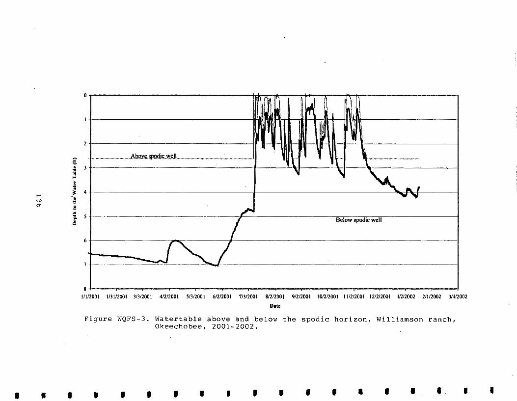
g .. :;; ~ .. ~ ..
....... ~ w
-.. "'
of! s ..Q ... 1:1. .. ~
I • •
0
2
............................... 1\l?.Q:V.Itll.n~i~ . .'W.!r.U ..................................... : ......................
3
4
5 Below spodic well
6
7
8
1/1/2001 1/31/2001 3/3/2001 4/2/2001 5/3/2001 6/2/2001 7/3/2001 8/2/2001 9/2/2001 10/2/2001 ll/2/2001 12/2/2001 112/2002 2/1/2002 3/4/2002
Date
Figure WQFS-3. Watertable above and below the spodic horizon, Williamson ranch, Okeechobee, 2001-2002.
I • ' I I I ' ' ' ' • • I • I I

-• ,."'"' -i
••
•
-•
•
--•
---•
•
-•
becomes much greater. The equipment blanks show that little or no cross contamination of samples occurred; phosphorus contents were near or below detection levels.
Review of the TP (digested) data indicated that its analyses had problems during some periods, particularly during 2001. The data did not follow the expected trends for the treatments. Fortunately, TP was also analyzed by ICAP (inductively-coupled argon plasma) spectroscopy for many samples, and these data follow the expected trends.
Only the last year (200 1) data are presented and used for analyzing the treatment effects because a startup effect of the treatments was observed in the data, i.e. it was clear the treatment effects had not reached equilibrium during the first two years. This decision was further supported by the total lack of runoff during 2000. This startup equilibrium effect was clearly evident in the surface water data where no treatment effects were observed until200 1. The well water samples appeared to come to equilibrium quicker.
Due to cattle traffic in the plots, it was observed that one or two temporary breaches of the plot berms between plots occurred which would have allowed some limited cross flow between the plots. These breaches, however, were repaired as soon as they were found. Though these breaches might have partially mixed the runoffs during one or two storm events, the overall responses to the individual treatments are not likely to be significantly affected over the length of the study and should have little influence on the lack of equilibrium being reached as stated above .
Total P. The water quality data by treatment are presented in Table WQFS-2 in the form of linear regression equations. The ICAP-TP data are used because these TP data were found to be more reliable for calibration hence also for EAAMOD simulation on P levels in water for the study. Table WQFS-2 shows that fertilizer Prates, compared to pH and EC, tended to have the largest coefficient of determination indicating that it is the most important factor associated with P levels in all types of water samples .
· EC. Specific conductance results clearly indicate that each of the amendments including P fertilizer increased specific conductance (Table WQFS-2). The treatment response trends were similar for all three sample types (deep and shallow groundwater and runoff). The gypsum amendment had the most dramatic response, due to its very high solubility in water, where higher levels of gypsum significantly increased conductivity levels. Calcium carbonate orCa lime also had a positive trend to conductivity. Fertilizer Prate appeared to have none to a slight negative trend with EC for the deep well data only, but not significantly. As anticipated, the shallow ground wells had the greatest response and the surface runoff samples the least for conductivity changes .
pH. There appears to be little differences between the treatments for pH (Table WQFS-2). The only response that appeared was a slight negative response (pH dropping with increased application rate) with rates of gypsum. This was for the shallow well samples only, and this was not significant. The pH for the surface runoff appeared to increase with Ca lime application rate, but again this was not significant.
137

...... w co
I I
Table WQFS-2. Relationships between pH, EC, or total P (TP) with Ca amendments or fertilizer Prates in surface runoff (Paddlewheels) and water samples above the spodic (Shallow wells) and below the spodic (Deep wells) horizon.
Depth/Treatment Water variables
pH EC (Jlmho cm-1) TP (Jlg L"1
)
Paddlewheels Equation R2 Equation R2 Equation R2
Ca carbonate Y= 0.039X + 6.420 0.0053 Y = -0.0013X + 61.57 5E-09 Y = -64.75X + 1349.0 0.0189 Gypsum Y = -0.049X + 6.682 0.0218 Y= 0.9835X + 63.15 0.0072 Y = - 6.86X + 1292.5 0.0002 Prates Y = -0.0003X + 6.585 0.0001 Y=: 0.31 02X + 50.17 0.0423 Y= 8.86X + 895.4 0.0485
Shallow wells
Ca carbonate Y = -0.050X + 4.953 0.0151 Y = 16.207X + 123.2 0.0966 Y = 282.71X + 5746.8 0.0143 Gypsum Y = -0.271X + 5.549 0.1554 Y = 77.380X + 140.1 0.1094 Y = 36.73X + 5221.4 0.0002 Prates Y = -0.006X + 5.029 0.0226 Y = 0.344X + 129.4 0.0072 Y= 8.86X + 895.4 0.0485
Deep wells
Ca carbonate Y = -0.047X + 4.487 0.0555 Y = 56.094X + 390.34 0.1614 Y = 182.02X + 908.1 0.0146 Gypsum Y = 0.186X + 4.505 0.1345 Y = 61.802X + 376.99 0.1135 Y = -268.62X + 1198.2 0.1476 Prates Y = 0.0004X + 4.431 0.0004 Y = -1.259X + 419.33 0.0086 Y= 28.90X- 40.1 0.2774
• • • I I I I • I • ' I • I • I I
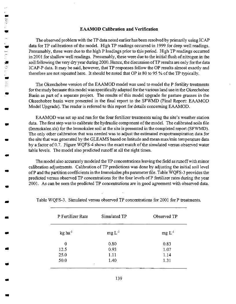
-•
•
---•
•
--•
•
•
•
•
• .. -
EAAMOD Calibration and Verification
The observed problem with the TP data noted earlier has been resolved by primarily using ICAP data for TP calibrations of the model. High TP readings occurred in 1999 for deep well readings . Presumably, these were due to the high P loadings prior to this period. High TP readings occurred in 2001 for shallow well readings. Presumably, these were due to the initial flush of nitrogen in the soil following the very dry year during 2000. Hence, the discussion ofTP results are only for the data ICAP-P data. It may be said, however, that TP responses follow the OP results almost exactly and therefore are not repeated here. It should be noted that OP is 80 to 95% of the TP typically.
The Okeechobee version of the EAAMOD model was used to model the P fertility treatments for the study because this model was specifically adapted for the various land use in the Okeechobee Basin as part of a separate project. The results of this model upgrade for pasture grasses in the Okeechobee basin were presented in the final report to the SFWMD (Final Report: EAAMOD Model Upgrade). The reader is referred to this report for details concerning EAAMOD.
EAAMOD was set up and run for the four fertilizer treatments using the site's weather station data. The first step was to calibrate the hydraulic component of the model. The calibrated soils file (Immokalee.sls) for the Immokalee soil at the site is presented in the completed r~port (SFWMD). The only other calibration that was needed was to adjust the estimated evapotranspiration data for the site that was generated by the GLEAMS based on latitude and mean maximin temperature data by a factor of0.7. Figure WQFS-4 shows the exact match of the simulated versus observed water table levels. The model also predicted runoff at all the right times.
The model also accurately modeled the TP concentrations leaving the field as runoff with minor calibration adjustments. Calibration of TP predictions was done by adjusting the initial soil level ofP and the partition coefficients in the Immokalee. phs parameter file. Table WQFS-3 provides the predicted versus observed TP concentrations for the four levels ofP fertilizer rates during the year 2001. As can be seen the predicted TP concentrations are in good agreement with observed data .
Table WQFS-3. Simulated versus observed TP concentrations for 2001 for P treatments .
P Fertilizer Rate Simulated TP Observed TP
kgha· 1 mgL· 1 mgL· 1
0 0.80 0.83 12.5 0.93 1.07 25.0 1.11 1.14 50.0 1.40 1.31
139
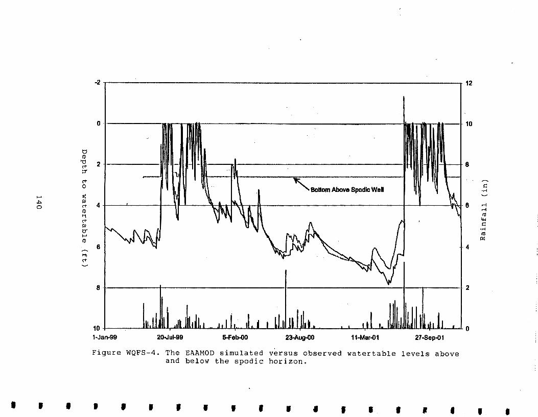
t:l ro '"d cT ::Y
cT 0
f-' :e:: .t:. 0.1 0 cT
ro t-1 cT 0.1 0' 1-' ro ........ I-tt cT
I • I
-2 12
0 ·I .. I... ...... r-r-Al I 10
2 IIi If 11-11 HI-ll\ k IHIIIIHII\1.1 I 8
1 ""- Bottom Above Spodlc WeD ~ ~ 4
.
6 (\ ·4
8 ~2
10 I III!IUIU, '"'·~~'""I .. J I I I~· Ita I I BI.UI Jl I Ull
1 J 9
r t • t I I t Ia l!ltii•Uillll•l II,Y I 1J 1 1 O - an- 9 ' · 20..Jul-99 5-Feb-00 23-Aug.OO 11-Mar.01 27·Sep-Q1
Figure WQFS-4. The EAAMOD simulated versus observed watertable levels above and below the spodic horizon.
' • I I I ' ' I ' I I • • •
c: ...... ........
r-1 r-1 ro
4-l c: ...... ro
p:::
I •

r':'• -•
• • .. ,;.
' -•
-•
•
-•
•
-.. •
•
.. •
Figure WQFS-5 shows the simulated versus observed TP data for zero P fertilizer rate treatment over the entire study period. The predicted TP concentrations are in good agreement with the observed data for zero P rates .
The calcium treatments were simulated by modifying the EAAMod P partitioning coefficients to represent the changes in P partitioning due to changes in pH (Table WQFS-4). The simulated values were highly correlated with the measured values; however, meaningful statistics on predictive abilities of the model due to Ca treatments cannot be made based on this limited data set.
Table WQFS-4. Simulated versus observed TP concentrations for 2001 for Ca treatments .
Ca amendment
Mgha- 1
0 2
4
Prate
kgha-1
50 50
50
Measured TP
mgL-1
1.31 1.29
1.06
Simulated TP (mg L- 1)
mgL-1
1.40 1.27
1.16
In order to determine whether the system had reached equilibrium, EAAMod was run for 20 years using 1999 weather data for each year. The treatment of 50 kglha P, 0 Mglha Ca, and 0 Mglha gypsum was used (Figure WQFS-6). The results show that at this P load, the TP outflow concentration will continue to rise for many years. This suggests that the limited number of years used for the treatments were not enough to evaluate their final impacts .
141
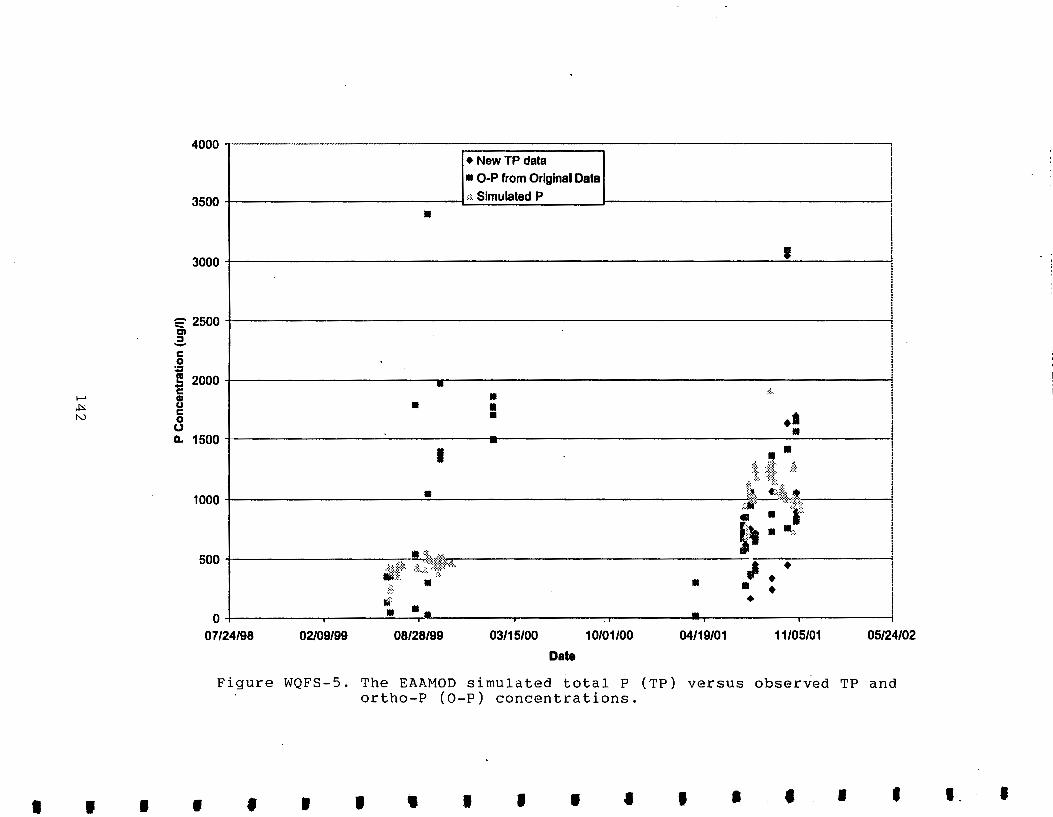
1-' ~ N
• I I
4000 y-------------------------~==============~~---------------------------• New TP data ~ • 0-P from Original Data I
~ ~~~p I ! •
3000 ' . !
~ 2500 g) :I -c 0 ::1 .s 2000 • c Gl u c 0 0
• • • • ::: ..
D. 1500 •• • - ...
: '~~.:t ' .. 1000 l' . .., 500 " • ::::~'t\i~i:~. J ••
• •
'
::. :::.
. ;!~:. • • • Iii'
0 • •
07/24/98 02/09/99 08/28/99 03/15/00 10/01/00 04/19/01 11/05/01 05/24/02
Date
Figure WQFS-5. The EAAMOD simulated total P (TP) versus observed TP and ortho-P (0-P) concentrations.
' I I • I • I I I I • I • I- I

I I I
>-3
"' 0 s:: c1" H1 ..... 0 ~
(1
0 ~ (1
I-" CD ~ ::s w c1"
11 Ill c1" 1-'· 0 ~
........ !3 lO ......... Ll -
I • I I I I I I I I •····. 1/i •.... :.!. ~, T. •.. ·; •
7 I
I --+- P 50 kg/ha, Ca 0 Mg/ha, Gypsum 0 Mg/ha I 6
4
3
2
1
0+-----~----~------r-----~-----r----~----~r-----~-----r----~
1999 2001 2003 2005 2007 2009
Year
2011 2013 2015 2017 2019
Figure WQFS-6. The EAAMOD simulated total P (TP) outflow concentrations for 20 years using the 1999 weather data each year.
.;: :J
PROJECT SUMMARY, CONCLUSIONS, AND RECOMMENDATIONS
Greenhouse Studies
Three greenhouse studies were conducted under the project primarily to help explain and/or confirm related field experiment results. Reference to relevant greenhouse observations and/or conclusions may be made in the field study summary.
The basic P retention capacity of the individual horizons of Immokalee fine sand and the influence ofCa amendments were determined in a greenhouse study (GS1). Potted individual soil horizons were used with no stargrass planted. Fertilizer Pat 0, 50, and 100 kg P ha-1 using triple superphosphate (TSP) and Ca amendments at 0 and 800 kg Ca ha·1 were applied to the potted Ap soils. The soils were then leached eight times sequentially, the Ap with deionized water, theE with Ap leachates, and the Bh with E leachates over a 220-day period.
The results showed that the P retention capacity of the horizons with no stargrass planted was in the order of Bh > Ap > E. The E horizon had almost zero P retention capacity as indicated by the leached P:applied P ratios around 1.0. This does not, however, mean that theE soils are devoid of P. Because the E soils are highly permeable, large P losses from lateral flow along this horizon in the field could be. expected should drainage ditches cut through it.
The granular lime materials, either calcium carbonate or dolomite, significantly reduced leaching P losses from the Ap horizon. Reduced P concentrations in Ap leachates due to liming could be attributed to slight increases in leachate pH. But with the lime's extremely low solubility, the undissolved lime particles on the surface of the potted Ap soils probably played the major role in reducing P leaching from the Ap horizon by precipitating P04 anions unto their surfaces. Calcium carbonate and dolomite were similarly effective in reducing P loss from the Ap horizon. With or without Ca amendments, 94 to 99 % of soil or fertilizer P that leached through the Ap and then through the E horizons was eventually retained in the Bh horizon.
Mined and byproduct gypsum, which are highly soluble, increased Ap leachate P and Ca concentrations and reduced leachate pH. Increase in Ca concentrations and reduction in pH could increase P04 mobility with Ca and P04 moving together as ion pairs. Substantial reduction in pH could also mobilize the micro elements in soils and make them significant factors in the leaching of P. In addition, S04 from gypsum could reduce adsorption ofP04, keep them in solution, and render them more vulnerable to leaching. Thus, the application of soil amendment that solubilizes into cations and anions in significant amounts could worsen the loss ofP through leaching.
Electrical conductivity, Ca, Mg, K, and AI were positively associated with P concentrations in Ap leachates; pH, Ca, AI, and Mn in E leachates; and Mn in Bh leachates. Leachate pH was negatively associated with P concentrations in Ap and E but not in Bh leachates.
144
---•
•
•
•
•
•
•
• •
•
.. •
•
•
•

-•
' -.. -.. -•
•
•
•
•
•
•
• .. -
The influence of cropping on Pretention by the individual horizons of Immokalee fine sand and the capacity of stargrass to utilize fertilizer P were determined in greenhouse study GS2-I. Potted soil horizon samples and commercial pure sand were planted to stargrass and fertilized at 100 kg P ha-1 using TSP. Bottom leachates were sampled ten times over a 24-week period.
The results indicated that plant-available soil Pin the Ap horizon plus fertilizer P applied at 100 kg P ha-1 were far in excess of the ability or capacity of stargrass to utilize them. For ten sampling events, leachate P concentrations ranged from 1.3 to 6.8 for Ap, 0.11 to 0.23 forE, 0.08 to 1.19 for Bh, and 0.0 to 0.17 mg L-1 for pure sand. Phosphorus concentrations in E, Bh, and pure sand leachates were not significantly different from one another at each sampling event. The relatively low E and pure sand leachate P concentrations point to the importance of pasture cropping in reducing or preventing fertilizer and/or soil P losses .
Stargrass forage yields in Ap, E, and Bh soils and in pure sand were not different from one another. Despite the different amounts of available P in the various media, such as between Ap and pure sand, P contents in stargrass regrowth forage remained within a narrow range of from 0.27 to 0.29 %. This would mean that unfertilized soils planted to stargrass with regrowth forage P contents within said range do not need any fertilizer P. Any application ofP besides being a waste of money would most likely increase P losses through leaching and/or runoff.
The third greenhouse study used potted reconstructed soil profile of Immokalee fine sand also planted to stargrass (GS2-II). Fertilizer Pat 0, 25, 50, and 100 kg P ha-1 were applied to pots without Ca amendments. Calcium carbonate, dolomite, or mined gypsum, all ground to powder, were applied at 0, 2 and 4 Mg ha-1 to pots fertilized at 100 kg P ha-1 with no Ca amendment as control.
The results showed that fine-ground Ca amendments failed to reduce P concentrations in soil water of reconstructed soil profile fertilized at 100 kg P ha- 1 sampled at the bottom of the Ap+E (shallow wells), Ap+E+Bh (deep wells), or Ap+E+Bh+C (bottom leachates) horizon profiles. There were also no meaningful effects of Ca amendments on leachate pH, EC, or Ca concentrations. It is doubtful that these non-effects could be attributed to the influence of stargrass alone because the grinding of the amendments into powder obliterated the important properties that differentiate gypsum from the lime materials, namely, solubility and pH effect. If grinding the lime materials indeed made them ineffective in reducing P losses through leaching, then P04 precipitation unto the surfaces of granular lime particles, as hypothesized in GS 1, could be the key to the effectiveness of lime in immobilizing P in soils .
Calcium amendments showed no effects on stargrass forage yield relative to the control. Limestone reduced P uptake by stargrass below that of the control indicating less available P to stargrass due, most probably, to some degree ofP precipitation. Phosphorus P contents ranged from 0.22 to 0.30. With no differences in yields, this would push P content down to 0.22 as a lower limit at which P fertilization would not result in increased forage yield.
Fertilizer P applied up to 100 kg P ha-1 had no effects on P concentrations in deep well (Ap+E+Bh) and bottom leachates (Ap+E+Bh+C). This could only be due to the strong retention
145

capacity of the Bh horizon for P. Although not generally significant, Pin shallow wells (Ap+E) tended to increase with increasing rates of fertilizer P. That P concentrations in the control (0 P, no Ca amendment, shallow wells) were not different from the P-fertilized pots strongly indicates that Immokalee fine sand has too much P to more than meet the needs of stargrass for P.
Fertilizer Prates had no effects on forage yield of stargrass. Again, this strongly indicates that Immokalee fine sand has too much P to meet needs for optimum forage yield. But fertilizer P increased forage P contents linearly from 0.20 to 0.30% asP rates increased from 0 to 50 kg P ha·1
•
Again, with no increase in forage yield, the lower limit is now 0.20 % P at which P fertilization would be unnecessary as it would not benefit forage yield.
The Ca:P ratios of3.1: 1 for the control and 2.2:1 for the highest fertilizer Prate were well within the desirable Ca:P ratio range of not less than 1:1 to not more than 7: 1. These high Ca:P ratios could be due to the leaching of P, but not Ca, out ofthe root zone upon watering reducing P uptake but keeping soil Ca uptake relatively unaffected.
Agronomic and Water Quality Field Experiments
Fertilizer P as TSP was applied annually at 0, 12.5, 25, and 50 kg P ha·1 to stargrass pasture from 1999 to 2001. Calcium carbonate or mined gypsum was applied at 0, 2 and 4 Mg ha· 1 to plots and fertilized at 50 kg P ha-1• Treatments were replicated four times.
In the field experiment, P fertilizer did not increase forage yields, as the two greenhouse studies did show, nor improve forage quality measures such as crude protein (CP) contents and in vitro organic matter digestibility (IVOMD). Forage from plots where no fertilizer P was applied for three crop years did not show any deterioration in forage yield and in quality on the third year. Forage yields were influenced more by crop year, which had distinctly different rainfall levels during the growing season, than by P fertilization.
Phosphorus fertilization increased P contents significantly. The three-year average P contents of regrowth forage ranged from 0.19 to 0.34% as fertilizer P increased from 0 to 50 kg P ha· 1 applied
•
•
--•
•
• •
•
•
• annually. With no increase in forage yield, the field results indicate that no P fertilizer is needed for a stargrass pastures having regrowth forage P contents of 0.19 % or more. These field results are supported by the data from the two greenhouse studies GS2-I and GS2-II.
Calcium increased only slightly resulting in the deterioration ofthe Ca:P ratio to levels that could be detrimental to animal growth and development and to feed efficiency. Phosphorus fertilization as low as 12.5 kg ha-1 reduced Ca:P ratio close to the acceptable lower limit of 1:1 just after three years of application. The highest rate of 50 kg ha· 1 reduced Ca:P ratio to less than 1 by the second year of application. At this rate ofP fertilization, Ca sources such as calcium carbonate or gypsum at the highest rate of 4 Mg ha· 1 applied at the beginning of the study failed to increase Ca:P ratio beyond the lower acceptable limit after three years of high P fertilization.
146
•
• •
•
•
•

•
-.. -•
-.. -•
•
• ..
-•
• •
•
Evaluation ofP uptake by stargrass indicated that P fertilization only helped to build up soil P at the rate of at least 0. 70 kg P for each kg of fertilizer P applied per ha per year with no agronomic benefits. The accounting of soil and fertilizer P in the three greenhouse studies supports such build up which could only increase the potential loss of soil P through runoff and/or leaching. Phosphorus fractionation of greenhouse (GS 1) and field samples indicates that Immokalee fine sand has already high soil P in Ap, E, and Bh horizons even without P fertilization .
Considering the major agronomic findings, it is concluded that stargrass on Immokalee fine sand does not need any P fertilization. Hence, it is recommended that IF AS re-evaluate its recommendation on P fertilization of stargrass and other similar improved pastures species on Immokalee fine sand .
With an Ap soil pH of 4.4, the forage yield data indicate that stargrass in the area may benefit from liming using calcium carbonate which showed some tendencies to increase forage yields. The potential oflime materials to reduce P losses through leaching (GS 1) would certainly be an added benefit to their on these soils. The greenhouse studies indicate that granular lime materials would be more effective to retain P in the soil than highly soluble fine-ground ones .
The water quality analysis indicates that the P fertility response for the stargrass is similar to what the previous bahiagrass study showed, that increased P application rates appear to exponentially increase soil-water P levels as fertilizer rates exceed grass uptake rates. Greenhouse study GS 1 demonstrated that increased P rates increased P concentrations in the Ap leachates. The runoff TP concentrations also increased with P fertilizer rate, but more linearly. The study also showed that the soil amendment Ca lime only slightly decreased TP concentration in runoff while the gypsum amendment appeared to have slightly increased TP concentrations. These tendencies were noted in greenhouse study GS 1 but in more pronounced and significant degrees .
The data also indicate that the field was probably not fully equilibrated to the treatment trials, which means that the treatment effects observed could possibly become even greater over more time . The dry conditions during the first two years of the study increased the equilibration time resulting in only the third year of data being useful for assessing the treatment effects. In spite of the equilibrium issue, the results clearly show that over fertilization will result in higher P losses . Though promising, the long term benefits of theCa lime amendment are not clear from this study due to the equilibrium effect, and therefore should be further investigated. Gypsum is clearly not a beneficial amendment for reducing P losses from pastureland.
After calibration, the EAAMOD model was able to accurately simulate the P fertilizer treatment effects observed at the site. The simulated and observed values for 2001 were highly correlated for the various phosphorous treatments. Regressing the simulated and observed TP outflow concentrations gave a slope of 1.01 and an R2 of 0.76 indicating a good trend and correlation between simulated and observed values. The model simulated the TP discharge concentration changes as influenced by P fertilizer rates, and therefore should be a useful tool for investigating other potential fertility BMPs on other soils and crops in the area .
147

The most important conclusion that can be drawn from all the studies is that Immokalee fine has too much plant-available P to require P fertilization of stargrass or, probably, other improved grass species as well. Hence, it is strongly recommended that IF AS reconsiders its P fertilizer recommendations for stargrass and similar improved grass species.
The study also demonstrated pasture cropping as a major method or practice to reduce, if not totally, prevent P losses through leaching and, possibly, also runoff.
In order to minimize soil and/or fertilizer P losses from agricultural lands, the following should be considered: (1) increase the capacity of the Ap horizon to retain P by use of appropriate soil amendments like limestone or dolomite, (2) prevent P-loaded water atop the Bh horizon, that is in theE horizon, from reaching into open ditches that drains into open bodies of waters or lakes, hence, construction of drainage ditches should be discouraged or when necessary must not go deeper than the depth of the Ap horizon, (3) allowing surface water time to leach through the Bh horizon by confining excess water in wetlands, and (4) leaving no significant portion ofland left uncovered or unplanted to pasture grasses.
The economic justification of applying lime solely to retain P in the soil profile in Spodosols does not appear to be warranted because, as long as P is not permitted to be lost through runoff and/or lateral flow through theE horizon into drainage ditches, 95 %of Ap soil P and at least 99 % of fertilizer P are eventually screened out from the percolating water or leachates and retained. It is, however, a bonus in a liming program to achieve desired soil pH. To use lime to retain fertilizer P in the Ap horizon in P-deficient soils to keep it readily accessible to plant roots may be worth the investment.
148
-•
-•
-• ..
•
•
•
•
•
• •
•
•
•
->·,;:·
-••
-•
--•
•
• .. • .. .. .. •
REFERENCES
Akinremi. 0.0., and C.M. Cho. 1991. Phosphate transport in calcium-saturated systems: II. Experimental results in a model system. Soil Sci. Soc. Am. J. 55:1282-1287.
Alcordo, IS, and JE Rechcigl. (1992). Use of solubility curves as a method to characterize phosphogypsum and its constituents. Common. Soil Sci. Plant Anal. 23(17-20):2595-2611.
Alcordo, IS, and JE Rechcigl. (1993). Phosphogypsum in agriculture: a review. In Advances in Agronomy, Vol. 49:55-118. D.L. Sparks (ed.). Academic Press. San Diego.
Alcordo, IS, JE Rechcigl, and RC Littell. 2002. Greenhouse evaluation of lime and gypsum materials for reducing phosphorus leaching in a Spodosol: Study 1: Individual soil horizons with no stargrass planted. (A sub-study of South Florida Water Management Project No. C-10201. Final Report. South Florida Water Management District, Okeechobee, FL.
Allen, Jr., L.H. 1988. Dairy-siting criteria and other options for wastewater management on high water-table soils. Soil and Crop Sci. Fla. Proc. 47:108-127.
Anderson, D.L., O.H. Tuovinen, A. Faber, and I. Ostrokowski. 1995. Use of soil amendments to reduce soluble phosphorus in dairy soils. Ecol. Eng. 5: 229-246.
Barade, M.D., and K.N. Chavan. 1998. Liming-induced changes in characteristics of Fluventic Ustropepts ofKonkan. J. Ind. Soc. Soil Sci. 46: 5-8 .
Bolan, N.S., R. Naidu, and S. Mahimairaja. 1994. Influence oflow-molecular-weight organic acids on the solubilization ofphosphates. Bioi. Fertil. Soils 18: 311-319 .
Botggaard, O.K., S.S. Jorgensen, J.P. Moberg, and B. Raben-Lange. J. Soil Sci. 41:443-449. Burgo a, B.A. 1989. Phosphorus spatial distribution, sorption, and transport in a Spodosol. (Ph.D. diss.). Univ. ofFlorida, Gainesville .
Bottcher, A.B., T.K. Tremwel, and K.L. Campbell. 1999. Phosphorus management in flatwood (Spodosols) soils. p. 405-423. In K.R. Reddy, G.A. O'Connor, and C.L. Schelske (eds.) Phosphorus biogeochemistry in subtropical ecosystems. Lewis Publishers, Boca Raton, FL.
Coutinho, J., M. Arrobas, and 0. Rodriguez. 1997. Effect ofcomposted sewage sludge amendment on soil nitrogen and phosphorus availability. Common. Soil Sci. Plant Nutr. 28: 1845-1857 .
Diaz, Q.A., K.R. Reddy, and P.A. Moore Jr. 1994. Solubility of inorganic phosphorus in stream water as influenced by pH and calcium concentration. Wat. Res. 28:1755-1763 .
149

Federico, A., K. Dickson, C. Kratzer, and F. Davis. 1981. Lake Okeechobee water quality studies and eutrophication assessment. Technical Publication 81-2, 270 pp. South Florida Water Management District, West Palm Beach, FL.
Ghani, A., and S.S.S. Rajan. 1996. Differential availability of partially sulphuric and phosphoric acidulated phosphate rocks. I. Plant response. Nutr. Cycl. Agroec. 47: 251-259.
Graetz, D.A., and V.D. Nair. 1995. Fate ofphosphorus in Florida Spodosols contaminated with cattle manure. Ecol. Eng. 5: 163-181.
Graetz, D.A., and V.D. Nair. 1999. Inorganic forms ofphosphorus in soils and sediments. p. 171-186. In K.R. Reddy, G.A. O'Connor, and C.L. Schelske (eds.) Phosphorus biogeochemistry in subtropical ecosystems. Lewis Publishers, Boca Raton, FL.
Gunsalus, B., E.G. Flaig, and G, Ritter. 1992. Effectiveness of agricultural best management practices implemented in the Taylor Creek/Nubbin Slough watershed and the Lower Kissimmee River Basin, The National Rural Clean Water Program Symposium. United States Environ. Protec. Ag., Washington, D.C. EPA/625/R-92/006. p.161-179.
He, Z.L., V.C. Baligar, D.C. Martens, K.D. Ritchey, and W.D. Kemper. 1996. Factors affecting phosphate rock dissolution in acid soil amended with liming materials and cellulose. Soil Sci. Soc. Am. J. 60: 1596-1601.
Holford, I.C.R., B.E. Schweitzer, and G.J. Crocker. 1994. Long-term effects of lime on soil phosphorus solubility and sorption in eight acidic soils. Austr. J. Soil Res. 32: 795-803.
lbrikci, H. 1993. Phosphorus availability for bahiagrass production on a Spodosol. Ph.D. diss. Univ. ofFlorida, Gainesville.
Kidder, G., E.A.Hanlon, and C. G. Chambliss. 1998. UP !IF AS standardized fertilization recommendations for agronomic crops. Fact Sheet SL-129, Soil and Water Science Dept., Florida Cooperative Management Service, IFAS, Univ. ofFlorida, Gainesville.
Lindsay, W.L. 1981. Solid phase-solution equilibria in soils. p. 183-202. In M. Stelly (ed.): Chemistry of soil environment. ASA Special Publ. No. 40. ASA, SSSA, Madison, WI.
Mansell, R.S.,Bloom, S.A., andP. Nkedi-Kizza. 1995. PhosphorustransportinSpodosols impacted by dairy waste. Ecol. Eng. 5: 281-299.
McDowell, L.R., J.H. Conrad, and F. Glen Hembry. 1993. Minerals for grazing ruminants, 2nd Ed., Animal Science Department, University of Florida, Gainesville, FL.
Mehlich, A. 1953. DeterminationofP, Ca,Mg, K, Na, andNH4. Soil TestingDiv. Publ. 1-53, North Carolina Dep. Agric., Raleigh, NC.
150
-..
•
--•
-•
-•
•
• .. •
•
•
-:II
' -
•
.. -.. •
•
-
Mongia, A.D., N.T. Singh, L.N. Mandai, and A. Guha. 1998. Effect of lime and phosphorus application on nutrient transformations in acid and acid sulphate soils under submergence. J. Ind. Soc. Soil Sci. 46: 18-22.
Mortvedt, J.J. 2000. Bioavailability of micronutrient. In M.E. Sumner (ed-in-chief) "Handbook of Soil Science." p. D-71 - D-88. CRC Press. Boca Raton.
Murphy, J., and J.P. Riley. 1962. A modified single solution method for the determination of phosphate in natural waters. Anal. Chim. Acta 27: 1244-1249.
Nair, V.M., D.A. Graetz, and K.M. Portier. 1995. Forms of phosphorus in soil profiles from dairies of South Florida. Soil Sci. Soc. Am. J. 59: 1244-1249.
Newman, S., and J.S. Robinson. 1999. Forms of organic phosphorus in water, soils, and sediments. p. 207-223. In K.R. Reddy, G.A. O'Connor, and C.L. Schelske (eds.) Phosphorus biogeochemistry in subtropical ecosystems. Lewis Publishers, Boca Raton, FL.
Peters, J .M., and N. T. Basta. 1996. Reduction of excessive bioavailable phosphorus in soils by using municipal and industrial wastes. J. Environ. Qual. 25: 1230-1241.
Phillips, I.R. 1998. Use of soil amendments to reduce nitrogen, phosphorus and heavy metal availability. J. Soil Contam. 7: 191-212.
Probert, M.E., M.G. Cannon, and W.S. Hicks. 1991. Effects ofliming and phosphorus on three soils from the wet coast ofNorth Queensland. Common. Soil Sci. Plant Anal. 21: 191-206.
Rechcigl, JE, and A.B. Bottcher. 1995. Fate of phosphorus on bahiagrass (Paspalum notatum) pastures. Ecol. Eng. 5: 247-259 .
Rechcigl, JE, A.B. Bottcher, and G. G. Payne. 1990. Development of fertilization practices for beef cattle pastures to minimize nutrient loss in runoff. Univ. of Florida IFAS Final Report to the South Florida Water Management District.
Rechcigl, JE, A.B. Bottcher, RC Littell, IS Alcordo, and L. Boruvka. 1999-200. Evaluation of limestone and gypsum for reducing phosphorus leaching and runoff from beef cattle forage . Annual Progress Report (March 1999-J anuary 2000). South Florida Water Management District Contract No. C-10201.
Rechcigl, JE, IS Alcordo, C.E. Roessler, and RC Littell. 1996. Influence ofphosphogypsum on forage yield and quality and on the environment in typical Florida Spodosol soils. Vol. I and II
• (Publ. No. 01-085-127). Florida Institute ofPhosphate Research, Bartow, FL.
•
• 151
-

Robertson, W.J., RC Jeffery, and I.R. McPharlin. 1997. Residues from bauxite-mining (red mud) increase phosphorus retention of a Joel sand without reducing yield of carrots. Common. Soil Sci. Plant Nutr. 28: 1059-1079.
SAS Institute. 1985. SAS procedures guide for personal computers. Version 6 ed. SAS Inst. Cary, NC.
Sharpley, A. 2000. Phosphorus availability. In M.E. Sumner (ed-in-chief) "Handbook of Soil Science." p. D-18- D-38. CRC Press. Boca Raton.
SFWMD. 1997. Surface water improvement and Management (SWIM) plan- Update for Lake Okeechobee. South Florida Water Management District. Okeechobee, FL..
Tunesi, Poggi, and Gessa. 1999. Phosphate adsorption and precipitation in calcareous soils: role of calcium ions in solution and carbonate materials. Nutr. Cycl. in Agroecosys. 53:219-227. Kluwer Academic Publishers. Netherlands.
USDA-SCS-DACS. 1984. Soil survey ofHardee county, Florida. Florida Dep. ofConsum. Serv., Tallahassee.
Wang,H.D., W.G. Harris,K.R. Reddy, and E.G. Flaig. 1995. Stability of phosphorus forms in dairyimpacted soils under simulated leaching. Ecol. Eng. 5: 209-227.
Walkley, A., and LA. Black. 1934. An examination ofthe Degtjareffmethod for determining soil organic matter and a proposed modification ofthe chromic titration method. Soil Sci. 37:29-38.
Ward, S.C., and R.N. Summers. 1993. Modifying sandy soils with the fine residue from bauxite refining to retain phosphorus and increase plant yield. Fert. Res. 36: 151-156.
Weast, R. C (Ed.). 1980-81. CRC Handbook of Chemistry and Physics. CRC Press, Inc. Boca Raton, FL.
Zhu, B., and A.K. Alva. 1994. The effect of gypsum amendment on transport of phosphorus in sandy soil. Water, Air, and Soil Poll. 78:375-382.
152
-•
-•
--...
•
.. -.. -•
•
•
.. •
•

-,,
--•
•
•
.. •
•
•
•
• .. • • ..
ACKNOWLEDGMENT
The authors hereby express their thanks and appreciations to the Williamson Cattle Company for use of its pasture for the study and for the assistance extended to them by its staff and to Ms. Cynthia D. Holley (Biological Scientist) and Mr. William S. Tewksbury (Project Technician) for their help in the conduct of the various aspects of the study.
153
•
•
-APPENDICES A: Water Sample Collection Protocol
•
• •
-.. -• •
.. • •
• 154 •
•
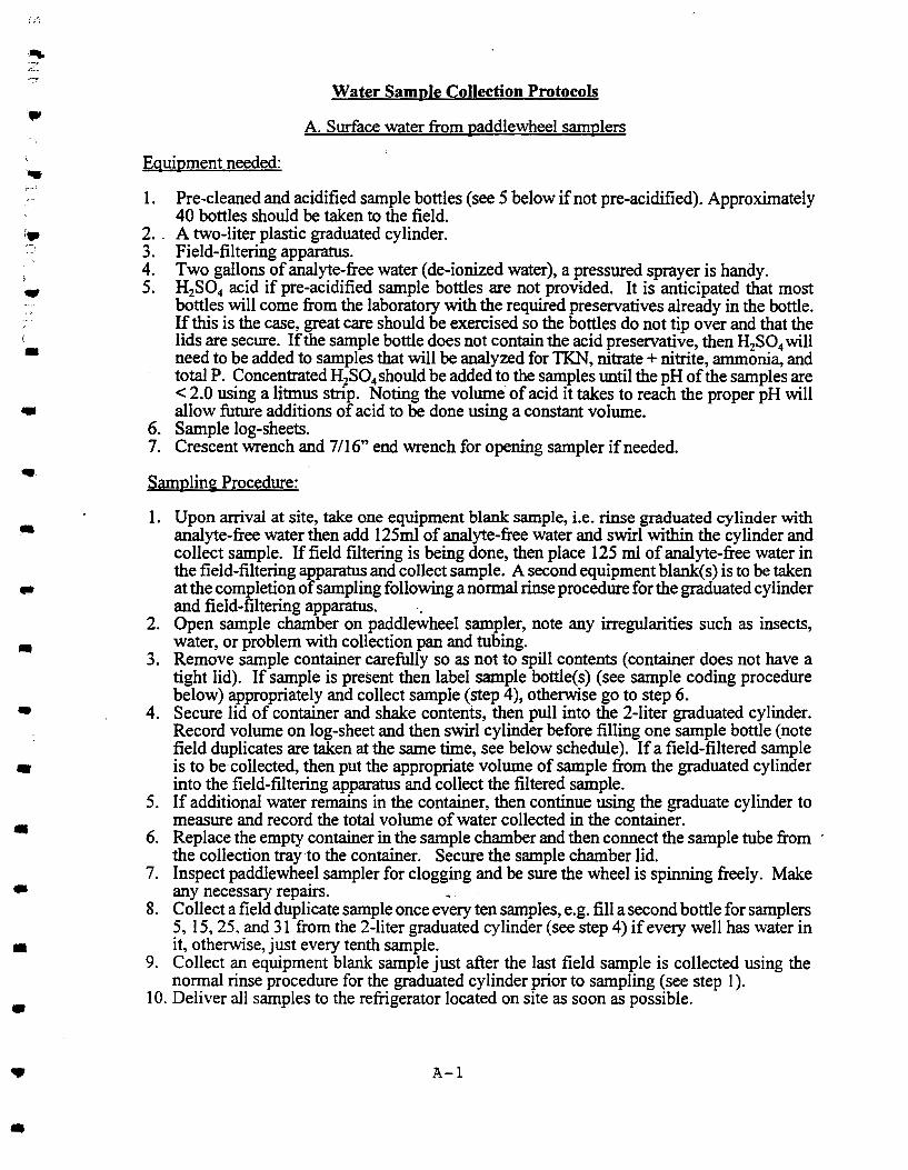
•
!· •,
•
•
..
.. •
-•
•
-•
•
.. •
Water Sample Collection Protocols
A. Surface water from paddlewheel samplers
Eguipment needed:
1. Pre-cleaned and acidified sample bottles (see 5 below if not pre-acidified). Approximately 40 bottles should be taken to the field.
2. _ A two-liter plastic graduated cylinder. 3. Field-filtering apparatus. 4. Two gallons of analyte-free water (de-ionized water), a pressured sprayer is handy. 5. H2SO4 acid if pre-acidified sample bottles are not provided. It is anticipated that most
bottles will come from the laboratory with the required preservatives already in the bottle. If this is the case, great care should be exercised so the bottles do not tip over and that the lids are secure. If the sample bottle does not contain the acid preservative, then H2S04 will need to be added to samples that will be analyzed for TKN, nitrate +nitrite, ammonia, and total P. Concentrated H2S04 should be added to the samples until the pH of the samples are < 2.0 using a litmus strip. Noting the volume· of acid it takes to reach the proper pH will allow future additions of acid to be done using a constant volume .
6. Sample log-sheets. 7. Crescent wrench and 7/16" end wrench for opening sampler if needed.
Sampling Procedure:
1. Upon arrival at site, take one equipment blank sample, i.e. rinse graduated cylinder with analyte-free water then add 125ml of analyte-free water and swirl within the cylinder and collect sample. If field filtering is being done, then place 125 ml of analyte-free water in the field-filtering apparatus and collect sample. A second equipment blank( s) is to be taken at the completion of sampling following a normal rinse procedure for the graduated cylinder and field-filtering apparatus. .
2. Open sample chamber on paddlewheel sampler, note any irregularities such as insects, water, or problem with collection pan and tubing .
3. Remove sample container carefully so as not to spill contents (container does not have a tight lid). If sample is present then label sample bottle(s) (see sample coding procedure below) appropriately and collect sample (step 4), otherwise go to step 6.
4. Secure lid of container and shake contents, then pull into the 2-liter graduated cylinder. Record volume on log-sheet and then swirl cylinder before filling one sample bottle (note field duplicates are taken at the same time, see below schedule). If a field-filtered sample is to be collected, then put the appropriate volume of sample from the graduated cylinder into the field-filtering apparatus and collect the filtered sample.
5. If additional water remains in the container, then continue using the graduate cylinder to measure and record the total volume of water collected in the container .
6. Replace the empty container in the sample chamber and then connect the sample tube from · the collection tray to the container. Secure the sample chamber lid.
7. Inspect paddlewheel sampler for clogging and be sure the wheel is spinning freely. Make any necessary repairs. _
8. Collect a field duplicate sample once every ten samples, e.g. fill a second bottle for samplers 5, 15, 25, and 31 from the 2-liter graduated cylinder (see step 4) if every well has water in it, otherwise, just every tenth sample .
9. Collect an equipment blank sample just after the last field sample is collected using the normal rinse procedure for the graduated cylinder prior to sampling (see step 1 ).
10. Deliver all samples to the refrigerator located on site as soon as possible .
A-1

B. Collection from subsurface ground water (wells)
Equipment needed:
1. Pre-cleaned and acidified sample bottles (see 5 below if not pre-acidified). Approximately 80 bottles should be taken to field.
2. Tubing and well pump. 3. Measuring tape or well sounder for measuring water levels. 4. Four gallons of analyte-free water (de-ionized water). 5. H2S04 acid if pre-acidified sample bottles are not provided. It is anticipated that most
bottles will come from the laboratory with the required preservatives already in the bottle. If this is the case, great care should be exercised so the bottles do not tip over and that the lids are secure. If the sample bottle does not contain the acid preservative, then H2S04 will need to be added to samples that will be analyzed for TKN, nitrate+ nitrite, ammonia, and total P. Concentrated H2S04 should be added to the samples until the pH of the samples are < 2.0 using a litmus strip. Noting the volume of acid it takes to reach the proper pH will allow future additions of acid to be done using a constant volume.
6. Sample log-sheets.
Sampling Procedure:
1. Upon arrival at site, take one equipment blank sample, i.e. rinse pump and tubing with analyte-free water then pump 125 ml of analyte-free water from a clean bottle to a sample bottle. If field filtering is being done, then place 125 ml of analyte-free water in the fieldfiltering apparatus and collect sample. A second equipment blank(s) is to be taken at the completion of sampling following a normal rinse procedure for the graduated cylinder and field-filtering apparatus.
2. Note any unusual occurrences at the wells.
Steps 3 through 7 are for well purging and water level measurements only. Note no samples are collected during this phase.
3. Measure water level in wells (from the same point on the top of the casings every time to the nearest 1/lOth foot minimum) using either a measuring tape or well sounder. Record depth to water on log-sheet. Rinse tape or sounder with analyte-free water before and after use.
4. Lower suction tube of peristaltic pump so that the intake is approximately one half inch from the bottom of the well. Pump three well volumes from the well or until dry, which ever is less. Rinse pump and tubing with analyte-free water before and after use. To determine the well volume use the following formula V=(0.04l)(d2)(h), where Vis volume in gallons, d is well diameter in inches, and h is water depth in feet.
5. Measure water level and purge all wells prior to sampling. 6. Return to the first well purged to start sample collection. Maximum time between purging
and sampling should be six hours. · 7. If sufficient sample is available in well, label sample bottle (see label code requirements
below) and collect sample by lowering the suction tube of peristaltic pump so that the intake is approximately one inch from the bottom of the well. It is critical that the tubing be rinsed with analyte-free water prior to being lowered into well. Start the pump and let at least 1 0 ml of sample go to waste prior to filling a temporary sample bottle (aliquot in this bottle is field filtered prior to being put into the labeled bottle) . If sufficient volume is available then additional water should be wasted prior to sampling. See item 5 under equipment above for acidification requirements. Once sufficient sample is drawn, tum off pump and remove tubing.
A-2
•
•
•
•
•
•
•
• •
• •
•
• •

,.,
iy
--•
-•
-•
•
•
• ..
•
8. Use field filtering apparatus if filtering is required- filtering is required only if sample is cloudy or muddy. The filtering apparatus and temporary sample bottle must be raised with analyte-free water between uses.
9. Collect a field duplicate sample once every ten samples, e.g. fill a second sample bottle from every tenth well just after the primary sample is collected.
10. Collect an equipment blank sample after every twenty samples. This sample is collected after the normal rinse procedure for the pump and tubing (see step 1 ).
11. Rinse pump and tubing with analyte-free water before going to the next well and record . sample data in log-sheet.
12. Deliver all samples to the refrigerator located on site as soon as possible or delivered directly to the UF laboratory in Ona.
C. Sample Preservation and Holding Times
Max Min. Parameter Container • Preservation Time Volume (ml) Ammonia P,G Cool, 4°C, 28 days 30
H2S04 to pH<2
TKN P,G Cool, 4°C, 28 days 30 H2S04 to pH<2
Nitrate+ P,G Cool, 4°C, 28 days 30 Nitrite H2S04 to pH<2
Phosphorus, P,G Cool, 4°C, 28 days 30 TDP & total H2S04 to pH<2
Phosphorous, P,G Cool, 4°C, 48 hrs 30 ortho field filtered
Solids, P,G Cool, 4°C, 7 days 100 total, dissolved, suspended, volatile
•p = Polyethylene, G=Glass
Sample preservation will be performed immediately upon collection and samples will be analyzed as soon as possible after collection (and always within the holding times shown).
The amount of H2S04 to be added to preserved samples will be based on experience oflaboratory personnel. Verification of correct pH will be done during the first sampling event fot each sample source using narrow range pH paper. An aliquot of sample poured into a disposable container, or a dummy sample in a disposable container will be tested for proper pH. The laboratory will supply all acid, containers to store acid, and disposable squeeze droppers to measure and transfer acid . Fresh preservatives will be obtained prior to each sampling event. Acid will be added to samples in small increments until the desired pH is reached. The required volumes of acid will be recorded in the field notebook and used during future sampling events. After the initial visit, only one sample
A-3

per each parameter will be checked unless an abnormal amount of acid had to be used during the initial testing. The same amount of acid will be added to appropriate equipment blanks as added to the corresponding sample.
All samples will be tightly sealed and placed in the refrigerator or into an ice chest that contains ice and bubble packaging to prevent breakage (if required). Each container will be placed upright. and surrounded with ice. A separate ice chest will be used for each site. The ice chest will periodically be drained of any melted ice, and additional ice will be added if necessary. After sampling is complete, or a separate segment is complete, the ice chest will be sealed with chain of custody tape, and will be shipped or transported by the project team to the lab.
D. Sampling Bottle Labeling
The following codes along with the date should be placed on each sample bottle:
Paddlewheel Sampler Code:
OPS for Okeechobee phosphorus study, P forpaddlewheel, 1-32 for plots, date of sampling, repeated plot number for duplicate; E for experimental (Alcordo) runoff samplers.
Groundwater Sample Code:
OPS for Okeechobee phosphorus study, D for deep well, S for shallow well, 1-32 for plots, date of sampling, and repeated plot number for duplicate.
A-4
• •
•
•
•
•
•
• •
..
.. • • •

-•
APPENDICES B: Quality Assurance: Chemical Analytical Procedures
i" ..
••
• .. •
•
.. •
155
•

• QUALITY ASSURANCE: CHEMICAL ANALYTICAL PROCEDURES
Analytical QA/QC. Quality assurance checks were used to ensure analytical data quality for water samples analysis. Since the main objective of the study is P and its forms, special attention was paid toP determination. On the ALPKEM automated analyzer, sample reruns, external standards and • spike samples were run every 20 samples. Detection and determination limits of the method were calculated from standard deviation results of a set ofblank samples. For detection limit, the standard deviation was multiplied by 3; for determination limit by 10. Values obtained were 2.5 and 8.3 J.Lg P L-1 or ppb for orthophosphate and 2.7 and 9.2 ppb for total phosphate. •
Figure 1 shows results of measurements of external standards. For both orthophosphate and total P, values obtained from 100 ppb P standard are in the range 10 % of expected value, which means • good accuracy. Data obtained from 10 ppb P standard in several cases dropped to about 80% of expected value. This concentration is already close to the determination limit of 10 ppb P of the method, and achieving 80 % of expected value may be considered quite accurate.
Figure1. Results of external standards for dissolved ortho-P (OP) and total P (TP).
OP - external standard 1 0 ppb P
12r---------------------------.
G. '8. 6 ...
...
4
2 J-Measured values -Expected values ...... +/-fO% 1
OP ·external standard 100ppb P
120 -:-----------------------------, '·······················································-·········!
100-" : 1
t.... ............................. ··························' so~
I ~ 60~
,. 40 J j -Measured values -Expected values ...... +/-10% i 1
20J
-
TP -external standard 1 0 ppb P
12r---------------------------~
" ~ :.:s-:-z-----===-- I 8
G. '8. 6 ...
\-Measured values -Expected values ....... +/-10% ' 4
2
I TP • external standard 1 OOppb P
120---1 100 ..................................................... ;.:.::.:::.:-:---·----·-
1 ................................. ~ ................. .
I i: .-~~~~--~~~~----~~
: - M!asured values _""""' "'"~ .....• , • .,, .I
Duplicate measurements were consistent, with relative difference not exceeding 10 % for both OP and TP on most samples with concentrations higher than the determination limits ofthe methods. Slightly lower precision of the TP determination can be explained by possible additional errors that could have been introduced during digestion of samples and standards. At concentrations lower than determination limit of the method the precision decreased. This is well apparent on the graph for OP. Since the samples for rerun were selected rap.domly only a few samples with concentrations below the determination limit were measured twice for TP. Absolute differences between duplicate measurements did not exceed 5 ppb P for both P forms.
B-1
·•
• • •
• • •
•
•
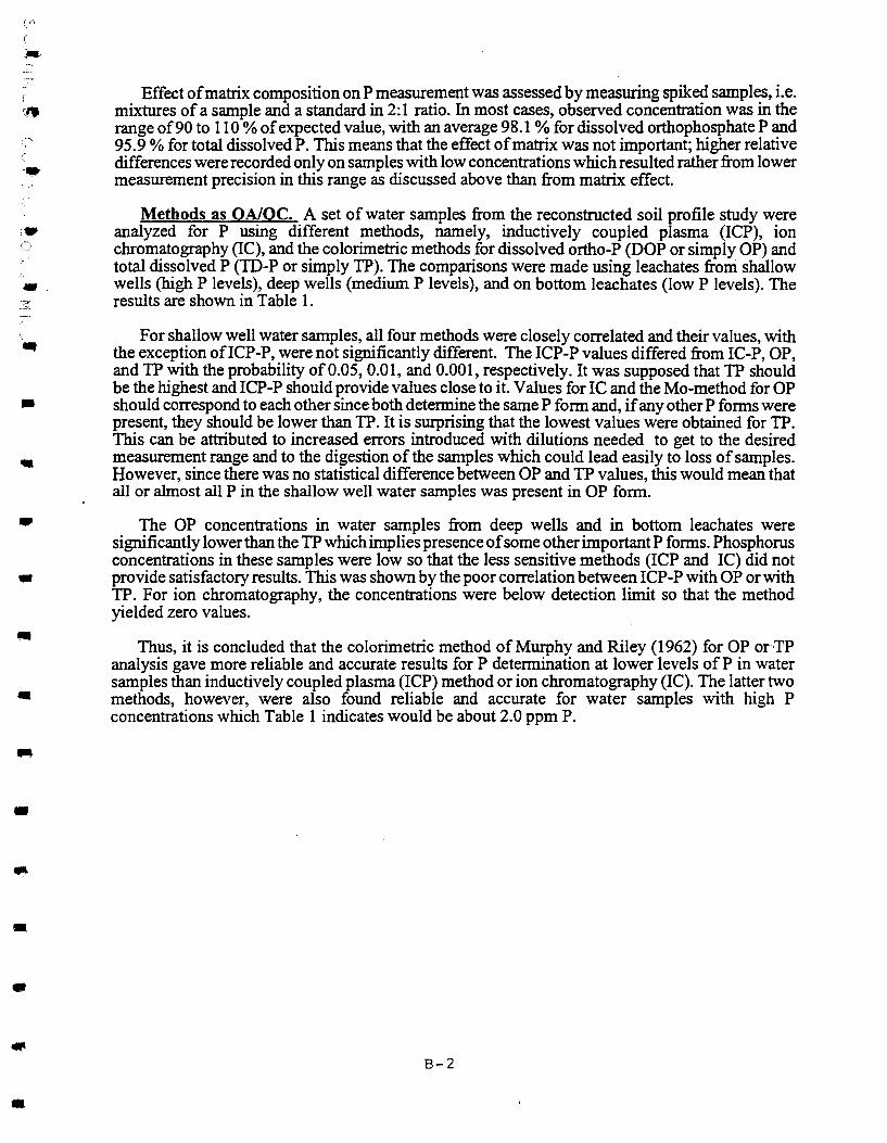
•• ,.,.,
!··.
•• . :.::,,
.. • .. •
•
.. •
•
•
•
•
Effect of matrix composition on P measurement was assessed by measuring spiked samples, i.e. mixtures of a sample and a standard in 2:1 ratio. In most cases, observed concentration was in the range of90 to 110% of expected value, with an average 98.1 %for dissolved orthophosphate P and 95.9 % for total dissolved P. This means that the effect of matrix was not important; higher relative differences were recorded only on samples with low concentrations which resulted rather from lower measurement precision in this range as discussed above than from matrix effect.
Methods as QA/OC. A set of water samples from the reconstructed soil profile study were analyzed for P using different methods, namely, inductively coupled plasma (ICP), ion chromatography (I C), and the colorimetric methods for dissolved ortho-P (DOP or simply OP) and total dissolved P (TD-P or simply TP). The comparisons were made using leachates from shallow wells (high P levels}, deep wells (medium P levels), and on bottom leachates (low P levels). The results are shown in Table 1 .
For shallow well water samples, all four methods were closely correlated and their values, with the exception ofiCP-P, were not significantly different. The ICP-P values differed from IC-P, OP, and TP with the probability of0.05, 0.01, and 0.001, respectively. It was supposed that TP should be the highest and ICP-P should provide values close to it. Values for IC and the Mo-method for OP should correspond to each other since both determine the same P form and, if any other P forms were present, they should be lower than TP. It is surprising that the lowest values were obtained for TP. This can be attributed to increased errors introduced with dilutions needed to get to the desired measurement range and to the digestion of the samples which could lead easily to loss of samples . However, since there was no statistical difference between OP and TP values, this would mean that all or almost all P in the shallow well water samples was present in OP form .
The OP concentrations in water samples from deep wells and in bottom leachates were significantly lower than the TP which implies presence of some other important P forms. Phosphorus concentrations in these samples were low so that the less sensitive methods (ICP and IC) did not provide satisfactory results. This was shown by the poor correlation between ICP-P with OP or with TP. For ion chromatography, the concentrations were below detection limit so that the method yielded zero values .
Thus, it is concluded that the colorimetric method of Murphy and Riley (1962) for OP orTP analysis gave more reliable and accurate results for P determination at lower levels of P in water samples than inductively coupled plasma (ICP) method or ion chromatography (I C). The latter two methods, however, were also found reliable and accurate for water samples with high P concentrations which Table 1 indicates would be about 2.0 ppm P .
B-2

-Table 1 Comparison and relationships of results of different methods for P determination: inductively coupled plasma (ICP), ion chromatography (IC), colorimetric method for dissolved " orthophosphate P (DOP) and for total dissolved P (TDP); average content and correlation coefficients.
•
• ICP IC DOP TDP
Shallow wells leachates
Average concentration, mg L-1 2.85 2.35 2.25 2.03
Number of samples 37 37 37 37 • Correlation ICP 1.000 coefficient • IC 0.927 1.000
DOP 0.950 0.871 1.000
TDP 0.892 0.839 0.947 1.000 • De~ wells leachates
Average concentration, mg L-1 0.19 0.00 0.040 0.068 • Number of samples 45 45 45 45
Correlation ICP 1.000 • coefficient IC
DOP 0.487 1.000
TDP 0.425 0.703 1.000
· Bottom leachates • Average concentration, mg L-1 0.12 0.00 0.006 0.031
Number of samples 52 52 52 52
Correlation ICP 1.000 coefficient
IC .. DOP 0.133 1.000
TOP 0.225 0.431 1.000
~
• B-3
•

APPENDICES C: Relations Between OP, TP, and ICAP-P '~ 1"·,:·
•
•
•
--.. .. •
•
.. 156
•

3.5
3 2.5
f 2 0 1.5 CD
1 E 0.5
0 -0.5
3
2.5
2 ...J a: 1.5 c 1-CD 1 E
0.5
0
Figure GS2. Relations between analytical fonns of P in leachates from reconstructed soil profile of Immokalee fine sand planted to stargrass fertilized at
50 kg Plha, all Ca amendments and depths. ICAP-P versus Ortho-P (OP)
y = 0.8311x- 0.0551
R2 =0.97 ~ .~.· ...... .... ""' . .. ~-
~ -----""" . .. .. .. .. ~= .
mg ICAP-P/L
Total dissolved P (TOP) versus ICAP-P
y = 0.7878x- 0.0109
R = 0.9215 +
-0.5 0.5 1 1.5 2 2.5 3 3.5
mg ICAP-PIL
Ortho-P (OP) versus Total dissolved P (TOP)
3~---------------------------------------------------------, 2.S+--Ly_=~0~.9~9~87~x~-~0~.0~0~3~7----------------------------~~~--------~
R2 =0.9455
i 2r-------------------------~~--~~pE~--~----------;
I~ • ~ 1.5 +-----------------~--·--~~~~~~------------------------~
lCD •
I E 1 +------------::...-.'-------------·--------1 I I 0.5 r-------~~~----------------------------------------------~
0 0.5 1 1.5
mg TDP/L
C-1
2 2.5 3
• • •
• •
•
• •
-•
• .. .. .. .. •· •
, .. APPENDICES D: Quality Assurance Samples: Duplicates
••
•
...
•
-•
•
.. •
.. •
• 157
•

•
D-1 .. ..

., ,. ,!···'
_,_ ..
'~ SampleiD
: ... ' ... ·.
1/31120001-
I= I= I= 5
502 1/3112000-•• o/o Error i'··J ····.
1/31120001-
I= I= • 15
I= • -~:>" 1502 1/31/2000-
--~~ Cfo Error -•• 25 1131/001
1-1767.71- 1971.61
25-2 1131/00 ... o/o Error
7/10/011 5P 2204.01 1739.01 .. 5P2 7/10/01 o/o Error -1.00 -1.00
7/10/011 1566.01 1195.01 15P 15P2 7/10/01
• Cfo Error -1.00 -1.00
7/10/011 490.11 16P 381.01
• 16P2 7/10/01 o/o Error -1.00 -1.00
- 7/10/011 778.11 643.31 25P 25P2 7/10/01
o/o Error -1.00 -1.00 .. 7127/011 1302.01 5P
• 5P2 7f2.7/01 1369.0 o/o Error 0.05
• 7127/011 I 15P ' 7951 15P2 7/27/01 880
o/o Error 0.11
•
• D-2
..

• Sample ID •
16P 7!27/011 15851 ..
16P2 7!27/01 %Error -1.00
• 25P 7!27/011 1~~1 25P2 7!27/01 • %Error 0.12
5P 816/011 13261 • 5P2 816/01 1468
%Error 0.11
• 15P 816/011 , ....
15P2 8/6/01 .... %Error •
16P 816/011 18201 16P2 816/01 1896
%Error 0.04
• 25P 816/011 =I 25P2 816/01
%Error 0.08 • 14P 9/10/011 I 30181 • 14P2 9/10/01 2211
%Error I
-0.27
26P 9/10/011 , ... 20401 26P2 9/10/01 %Error ...
10/12/011 I 1=1
l
5P - • 5P2 10/12/01 %Error 0.27
... 5P 10131/011 1230j
5P2 10131/01 11571 o/o Error -0.06 •
D-3

~--~"
.•. ._.,
·• Sample 10
-15P 10131/011 1~:1 - 15P2 10131/01
i·._. %Error -0.12 -·-
'a 25P 10/31/011 16471 25P2 10/31/01 155~
%Error -0.05 -•
•
-•
· .
••
•
...
•
•
• D-4
•

•
•
• •
•
• •
•
•
•
.. • • • •
•
•