
Final Colorado Greenhouse Gas Inventory and Reference Case
103
Colorado GHG Inventory and Reference Case Projection CCS, October 2007 Final Colorado Greenhouse Gas Inventory and Reference Case Projections 1990-2020 Center for Climate Strategies October 2007 Principal Authors: Randy Strait, Steve Roe, Alison Bailie, Holly Lindquist, Alison Jamison, Ezra Hausman, Alice Napoleon
Transcript of Final Colorado Greenhouse Gas Inventory and Reference Case
Colorado GHG Inventory and Reference Case Projection CCS, October 2007
Final Colorado Greenhouse Gas Inventory and
Reference Case Projections 1990-2020
Center for Climate Strategies October 2007
Principal Authors: Randy Strait, Steve Roe, Alison Bailie, Holly Lindquist, Alison Jamison, Ezra Hausman, Alice Napoleon

Colorado GHG Inventory and Reference Case Projection CCS, October 2007
ii Center for Climate Strategies www.climatestrategies.us
Colorado GHG Inventory and Reference Case Projection CCS, October 2007
iii Center for Climate Strategies www.climatestrategies.us
Executive Summary
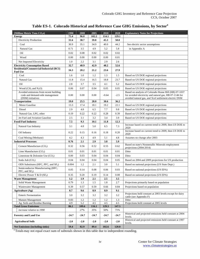
This report presents a summary of Colorado’s anthropogenic greenhouse gas (GHG) emissions and sinks (carbon storage) from 1990 to 2020. The Center for Climate Strategies (CCS) prepared a preliminary draft GHG emissions inventory and reference case projection for the Colorado Department of Public Health and Environment (CDPHE) through an effort of the Western Regional Air Partnership (WRAP).1 The preliminary draft report was provided to the Climate Action Panel (CAP) (and its Policy Work Groups [PWGs]) of the Colorado Climate Project to assist the CAP in understanding past, current, and possible future GHG emissions in Colorado, and thereby inform the policy option development process. The CAP and the PWGs provided comments for improving the reference case projections. This report documents the revised inventory and reference case projections incorporating comments as approved by the CAP.2 Colorado’s anthropogenic GHG emissions and anthropogenic/natural sinks (carbon storage) were estimated for the period from 1990 to 2020. Historical GHG emissions estimates (1990 through 2005)3 were developed using a set of generally accepted principles and guidelines for state GHG emissions inventories, relying to the extent possible on Colorado-specific data and inputs. The reference case projections (2006–2020) are based on a compilation of various existing Colorado and regional projections of electricity generation, fuel use, and other GHG-emitting activities, along with a set of simple, transparent assumptions described in Appendixes A through I of this report. Table ES-1 provides a summary of historical (1990 to 2005) and reference case projection (2010 and 2020) GHG emissions for Colorado. In 2005, on a gross emissions consumption basis (i.e., excluding carbon sinks), Colorado accounted for approximately 116 million metric tons (MMt) of CO2e emissions, an amount equal to 1.6% of total United States (US) gross GHG emissions. On a net emissions basis (i.e., including carbon sinks), Colorado accounted for approximately 89 MMtCO2e of emissions in 2005, an amount equal to 1.4% of total US net GHG emissions.4 Colorado’s GHG emissions are rising more quickly than those of the nation as a whole.5 1 Draft Colorado Greenhouse Gas Inventory and Reference Case Projections, 1990–2020, prepared by the Center for Climate Strategies for the Colorado Department of Public Health and Environment (CDPHE) through an effort of the Western Regional Air Partnership, January 2007. 2 Final Colorado Greenhouse Gas Inventory and Reference Case Projections, 1990–2020, prepared by the Center for Climate Strategies for the Climate Action Panel of the Colorado Climate Project, October 2007. 3 The last year of available historical data varies by sector; ranging from 2000 to 2005. 4 National emissions from Inventory of US Greenhouse Gas Emissions and Sinks: 1990-2005, April 2007, US EPA #430-R-07-002, (http://www.epa.gov/climatechange/emissions/usinventoryreport.html). 5 Gross emissions estimates only include those sources with positive emissions. Carbon sequestration in soils and vegetation is included in net emissions estimates. All emissions reported in this section for Colorado reflect consumption-based accounting (including emissions from electricity imports). On a national basis, little difference exists between production-based and consumption-based accounting for GHG emissions because net electricity imports are less than 1% of national electricity generation.
Colorado GHG Inventory and Reference Case Projection CCS, October 2007
iv Center for Climate Strategies www.climatestrategies.us
Table ES-1. Colorado Historical and Reference Case GHG Emissions, by Sectora
(Million Metric Tons CO2e) 1990 2000 2005 2010 2020 Explanatory Notes for Projections Energy 75.4 96.0 102.2 114.1 129.1 Electricity Production 31.6 38.7 39.8 45.3 50.0
Coal 30.9 35.1 34.9 40.0 44.2 See electric sector assumptions
Natural Gas 0.71 3.5 4.9 5.2 5.8 in Appendix A
Oil 0.02 0.08 0.02 0.02 0.02
Wood 0.00 0.00 0.00 0.00 0.01
Net Imported Electricity 1.0 2.2 3.1 2.9 2.6 Electricity Consumption Based 32.7 40.9 42.9 48.2 52.6 Residential/Commercial/Industrial (RCI) Fuel Use 16.3 20.2 21.2 23.6 27.9
Coal 1.6 1.0 1.2 1.3 1.5 Based on US DOE regional projections
Natural Gas 11.8 15.4 16.5 18.8 23.7 Based on US DOE regional projections
Oil 2.8 3.7 3.5 4.1 5.2 Based on US DOE regional projections
Wood (CH4 and N2O) 0.06 0.07 0.04 0.05 0.05 Based on US DOE regional projections
Avoided emissions from recent building
code and demand-side management (DSM) initiatives
0.00 0.00 0.00 -0.64 -2.5 Based on analysis of Colorado House Bill (HB) 07-1037 for avoided electricity and natural gas, HB 07-1146 for avoided natural gas, and Xcel settlement electric DSM
Transportation 19.0 25.5 28.0 30.6 36.2 Motor Gasoline 13.3 17.4 18.1 19.2 22.1 Based on US DOE regional projections
Diesel 2.9 4.8 6.5 7.7 9.8 Based on US DOE regional projections Natural Gas, LPG, other 0.19 0.22 0.22 0.28 0.39 Based on US DOE regional projections Jet Fuel and Aviation Gasoline 2.5 3.1 3.2 3.4 3.9 Based on US DOE regional projections Fossil Fuel Industry 7.5 9.3 10.1 11.8 12.3
Natural Gas Industry 3.1 4.8 5.0 6.5 7.3 Increase based on current trend to 2009, then US DOE to 2020
Oil Industry 0.22 0.15 0.16 0.18 0.20 Increase based on current trend to 2009, then US DOE to 2020
Coal Mining (Methane) 4.2 4.3 4.9 5.1 4.8 Assumes no change after 2003 Industrial Processes 0.76 2.1 2.9 3.8 5.9
Cement Manufacture (CO2) 0.32 0.56 0.52 0.55 0.62 Based on state's Nonmetallic Minerals employment projections (2004-2014)
Lime Manufacture (CO2) 0.01 0.01 0.01 0.01 0.01 Ditto
Limestone & Dolomite Use (CO2) 0.00 0.03 0.04 0.04 0.04 Ditto
Soda Ash (CO2) 0.04 0.04 0.04 0.04 0.05 Based on 2004 and 2009 projections for US production
ODS Substitutes (HFC, PFC, and SF6) 0.004 1.2 2.1 3.0 5.1 Based on national projections (US State Dept.)
Semiconductor Manufacturing (HFC, PFC, and SF6)
0.05 0.14 0.08 0.06 0.03 Based on national projections (US EPA)
Electric Power T & D (SF6) 0.35 0.20 0.19 0.14 0.08 Based on national projections (US EPA) Waste Management 1.2 1.9 2.1 2.5 3.5 Solid Waste Management 0.79 1.3 1.5 1.8 2.7 Projections primarily based on population
Wastewater Management 0.39 0.57 0.59 0.66 0.84 Projections based on population Agriculture (Ag) 8.7 9.6 8.9 8.9 9.1
Enteric Fermentation 3.0 3.2 3.2 3.2 3.2 Projections held constant at 2003 levels except for dairy cattle (see Appendix F)
Manure Management 0.83 1.2 1.2 1.2 1.3 Ditto Ag. Soils and Residue Burning 4.9 5.2 4.5 4.5 4.5 Projections held constant at 2005 levels Total Gross Emissions 86.1 109.6 116.1 129.3 147.5 increase relative to 1990 27% 35% 50% 71%
Forestry and Land Use -24.7 -24.7 -24.7 -24.7 -24.7 Historical and projected emissions held constant at 2004 levels.
Agricultural Soils -2.0 -2.0 -2.0 -2.0 -2.0 Historical and projected emissions held constant at 1997 levels.
Net Emissions (including sinks) 59.4 82.9 89.4 102.6 120.8 a Totals may not equal exact sum of subtotals shown in this table due to independent rounding.
Colorado GHG Inventory and Reference Case Projection CCS, October 2007
v Center for Climate Strategies www.climatestrategies.us
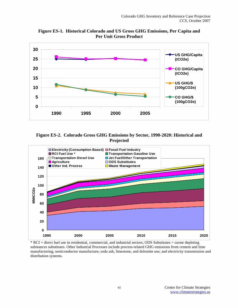
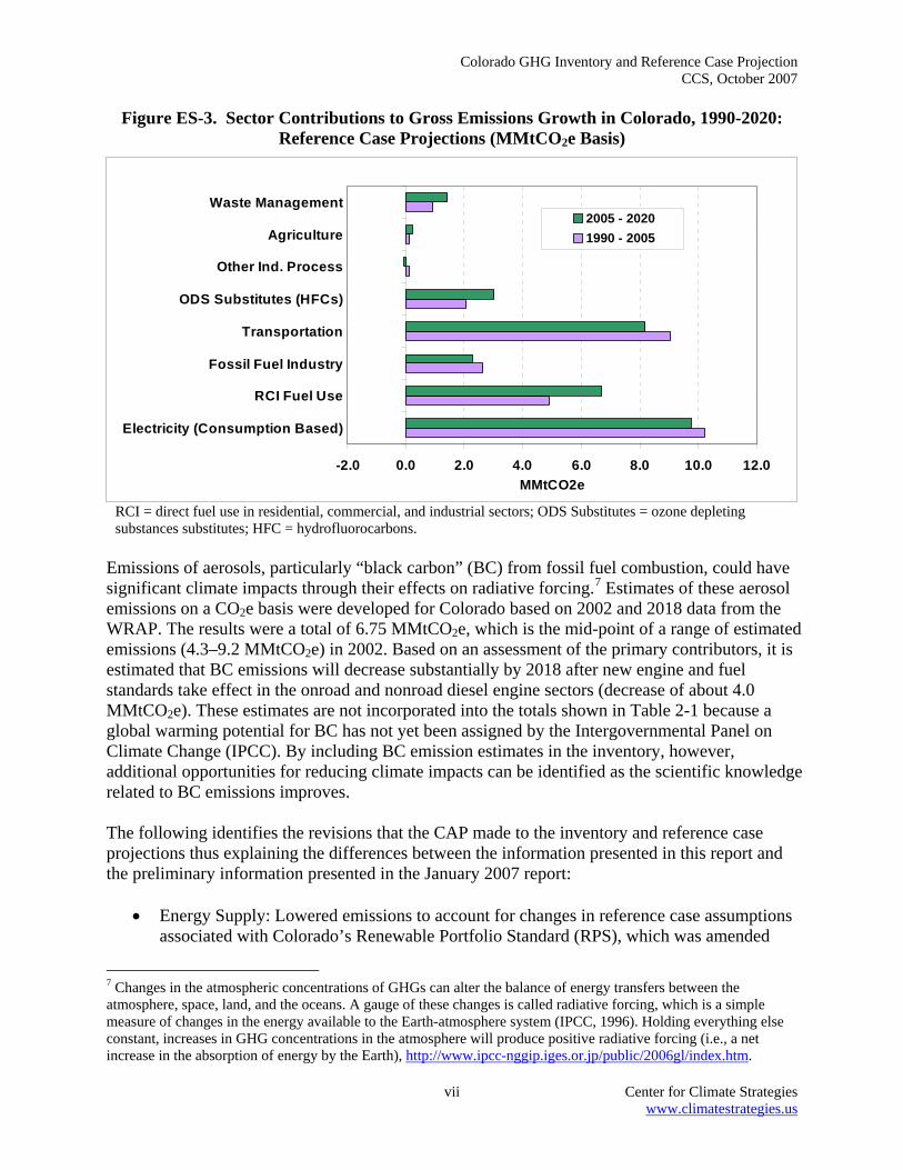
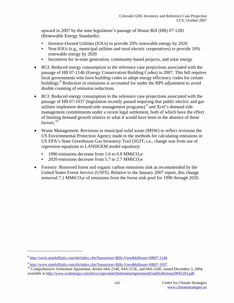
From 1990 to 2005, Colorado’s gross GHG emissions were up 35% while national gross emissions rose by 16% during this period. Much of Colorado’s emissions growth can be attributed to its population growth. From 1990 to 2005, Colorado’s population grew by 43% as compared with a national population growth of 19%. Figure ES-1 illustrates the state’s emissions per capita and per unit of economic output. Colorado’s per capita emission rate is slightly more than the national average of 25 MtCO2e/year. Between 1990 and 2005, per capita emissions in Colorado and national per capita emissions have changed relatively little. Economic growth exceeded emissions growth in Colorado throughout the 1990–2005 period. From 1990 to 2005, emissions per unit of gross product dropped by 40% nationally, and by 54% in Colorado.6 Electricity use and transportation are the state’s principal GHG emissions sources. Together, the combustion of fossil fuels for electricity generation and in the transportation sector accounted for 61% of Colorado’s gross GHG emissions in 2005. The remaining use of fossil fuels—natural gas, oil products, and coal—in the residential, commercial, and industrial (RCI) sectors, plus the emissions from fossil fuel production, constituted another 27% of total state emissions in 2005. As illustrated in Figure ES-2 and shown numerically in Table ES-1, under the reference case projections, Colorado’s gross GHG emissions continue to grow, and are projected to climb to 148 MMtCO2e by 2020, reaching 71% above 1990 levels. Overall, the average annual projected rate of emissions growth in Colorado is 1.6% per year from 2005 to 2020. As shown in Figure ES-3, demand for electricity is projected to be the largest contributor to future emissions growth accounting for about 36% of total gross GHG emissions in 2020, followed by emissions associated with transportation (25%), RCI fossil fuel use (19%), and fossil fuel production (8%) Some data uncertainties exist in this inventory, and particularly in the reference case projections. Key tasks for future refinement of the inventory and projections include review and revision of key drivers (such as electricity, fossil fuel production, and transportation fuel use growth rates) that will be major determinants of Colorado’s future GHG emissions. These growth rates are driven by uncertain economic, demographic, and land use trends (including growth patterns and transportation system impacts), all of which deserve closer review and discussion. Perhaps the variable with the most important implications for GHG emissions is the type and number of power plants that will be built in Colorado between now and 2020. The assumptions on VMT and air travel growth also have large impacts on projected GHG emissions growth in the state. Finally, uncertainty remains on estimates for historic and projected GHG sinks from forestry, which can greatly affect the net GHG emissions attributed to Colorado.
6 Based on gross domestic product by state (millions of current dollars), available from the US Bureau of Economic Analysis, http://www.bea.gov/regional/gsp/. The national emissions used for these comparisons are based on 2005 emissions, http://www.epa.gov/climatechange/emissions/usinventoryreport.html.
Colorado GHG Inventory and Reference Case Projection CCS, October 2007
vi Center for Climate Strategies www.climatestrategies.us
Figure ES-1. Historical Colorado and US Gross GHG Emissions, Per Capita and Per Unit Gross Product
0
5
10
15
20
25
30
1990 1995 2000 2005
US GHG/Capita(tCO2e)
CO GHG/Capita(tCO2e)
US GHG/$(100gCO2e)
CO GHG/$(100gCO2e)
Figure ES-2. Colorado Gross GHG Emissions by Sector, 1990-2020: Historical and Projected
0
20
40
60
80
100
120
140
160
1990 2000 2005 2010 2015 2020
MM
tCO
2e
Electricity (Consumption Based) Fossil Fuel IndustryRCI Fuel Use * Transportation Gasoline UseTransportation Diesel Use Jet Fuel/Other TransportationAgriculture ODS SubstitutesOther Ind. Process Waste Management
* RCI = direct fuel use in residential, commercial, and industrial sectors; ODS Substitutes = ozone depleting substances substitutes. Other Industrial Processes include process-related GHG emissions from cement and lime manufacturing; semiconductor manufacture; soda ash, limestone, and dolomite use; and electricity transmission and distribution systems.
Colorado GHG Inventory and Reference Case Projection CCS, October 2007
vii Center for Climate Strategies www.climatestrategies.us
Figure ES-3. Sector Contributions to Gross Emissions Growth in Colorado, 1990-2020: Reference Case Projections (MMtCO2e Basis)
-2.0 0.0 2.0 4.0 6.0 8.0 10.0 12.0
Electricity (Consumption Based)
RCI Fuel Use
Fossil Fuel Industry
Transportation
ODS Substitutes (HFCs)
Other Ind. Process
Agriculture
Waste Management
MMtCO2e
2005 - 20201990 - 2005
RCI = direct fuel use in residential, commercial, and industrial sectors; ODS Substitutes = ozone depleting substances substitutes; HFC = hydrofluorocarbons.
Emissions of aerosols, particularly “black carbon” (BC) from fossil fuel combustion, could have significant climate impacts through their effects on radiative forcing.7 Estimates of these aerosol emissions on a CO2e basis were developed for Colorado based on 2002 and 2018 data from the WRAP. The results were a total of 6.75 MMtCO2e, which is the mid-point of a range of estimated emissions (4.3–9.2 MMtCO2e) in 2002. Based on an assessment of the primary contributors, it is estimated that BC emissions will decrease substantially by 2018 after new engine and fuel standards take effect in the onroad and nonroad diesel engine sectors (decrease of about 4.0 MMtCO2e). These estimates are not incorporated into the totals shown in Table 2-1 because a global warming potential for BC has not yet been assigned by the Intergovernmental Panel on Climate Change (IPCC). By including BC emission estimates in the inventory, however, additional opportunities for reducing climate impacts can be identified as the scientific knowledge related to BC emissions improves. The following identifies the revisions that the CAP made to the inventory and reference case projections thus explaining the differences between the information presented in this report and the preliminary information presented in the January 2007 report:
• Energy Supply: Lowered emissions to account for changes in reference case assumptions associated with Colorado’s Renewable Portfolio Standard (RPS), which was amended
7 Changes in the atmospheric concentrations of GHGs can alter the balance of energy transfers between the atmosphere, space, land, and the oceans. A gauge of these changes is called radiative forcing, which is a simple measure of changes in the energy available to the Earth-atmosphere system (IPCC, 1996). Holding everything else constant, increases in GHG concentrations in the atmosphere will produce positive radiative forcing (i.e., a net increase in the absorption of energy by the Earth), http://www.ipcc-nggip.iges.or.jp/public/2006gl/index.htm.
Colorado GHG Inventory and Reference Case Projection CCS, October 2007
viii Center for Climate Strategies www.climatestrategies.us
upward in 2007 by the state legislature’s passage of House Bill (HB) 07-1281 (Renewable Energy Standards):
• Investor-Owned Utilities (IOUs) to provide 20% renewable energy by 2020 • Non-IOUs (e.g., municipal utilities and rural electric cooperatives) to provide 10%
renewable energy by 2020 • Incentives for in-state generation, community-based projects, and solar energy
• RCI: Reduced energy consumption in the reference case projections associated with the passage of HB 07-1146 (Energy Conservation Building Codes) in 2007. This bill requires local governments who have building codes to adopt energy efficiency codes for certain buildings.8 Reduction in emissions is accounted for under the RPS adjustment to avoid double counting of emission reductions.
• RCI: Reduced energy consumption in the reference case projections associated with the passage of HB 07-1037 (legislation recently passed requiring that public electric and gas utilities implement demand-side management programs) 9 and Xcel’s demand side management commitments under a recent legal settlement, both of which have the effect of limiting demand growth relative to what it would have been in the absence of these factors.10
• Waste Management: Revisions to municipal solid waste (MSW) to reflect revisions the US Environmental Protection Agency made to the methods for calculating emissions in US EPA’s State Greenhouse Gas Inventory Tool (SGIT; i.e., change was from use of regression equations to LANDGEM model equation):
• 1990 emissions decrease from 1.6 to 0.8 MMtCO2e • 2020 emissions decrease from 5.7 to 2.7 MMtCO2e
• Forestry: Removed forest soil organic carbon emissions sink as recommended by the United States Forest Service (USFS). Relative to the January 2007 report, this change removed 7.1 MMtCO2e of emissions from the forest sink pool for 1990 through 2020.
8 http://www.statebillinfo.com/sbi/index.cfm?fuseaction=Bills.View&billnum=HB07-1146. 9 http://www.statebillinfo.com/sbi/index.cfm?fuseaction=Bills.View&billnum=HB07-1037. 10 Comprehensive Settlement Agreement, docket 04A-214E, 04A-215E, and 04A-216E, issued December 3, 2004, available at http://www.xcelenergy.com/docs/corpcomm/SettlementAgreementFinalDraftclean20041203.pdf.
Colorado GHG Inventory and Reference Case Projection CCS, October 2007
ix Center for Climate Strategies www.climatestrategies.us
Table of Contents
Executive Summary ....................................................................................................................... iii Acronyms and Key Terms .............................................................................................................. x Acknowledgements...................................................................................................................... xiv Summary of Findings...................................................................................................................... 1
Introduction................................................................................................................................. 1 Colorado Greenhouse Gas Emissions: Sources and Trends ........................................................... 2
Historical Emissions ................................................................................................................... 4 Overview................................................................................................................................. 4 A Closer Look at the Two Major Sources: Electricity and Transportation ............................ 6
Reference Case Projections......................................................................................................... 7 CAP Revisions ............................................................................................................................ 9 Key Uncertainties and Next Steps ............................................................................................ 10 Approach................................................................................................................................... 10
General Methodology ........................................................................................................... 10 General Principles and Guidelines........................................................................................ 11
Appendix A. Electricity Use and Supply................................................................................... A-1 Appendix B. Residential, Commercial, and Industrial (RCI) Fuel Combustion ....................... B-1 Appendix C. Transportation Energy Use................................................................................... C-1 Appendix D. Industrial Processes .............................................................................................. D-1 Appendix E. Fossil Fuel Industries.............................................................................................E-1 Appendix F. Agriculture .............................................................................................................F-1 Appendix G. Waste Management .............................................................................................. G-1 Appendix H. Forestry................................................................................................................. H-1 Appendix I. Inventory and Forecast for Black Carbon................................................................I-1 Appendix J. Greenhouse Gases and Global Warming Potential Values: Excerpts from the
Inventory of U.S. Greenhouse Emissions and Sinks: 1990-2000........................... J-1
Colorado GHG Inventory and Reference Case Projection CCS, October 2007
x Center for Climate Strategies www.climatestrategies.us
Acronyms and Key Terms
AEO – Annual Energy Outlook, EIA
Ag – Agriculture
bbls – Barrels
BC – Black Carbon*
Bcf – Billion cubic feet
BLM – United States Bureau of Land Management
BOD – Biochemical Oxygen Demand
BTU – British thermal unit
C – Carbon*
CaCO3 – Calcium Carbonate
CAP – Climate Action Panel
CBM – Coal Bed Methane
CCS – Center for Climate Strategies
CDOT – Colorado Department of Transportation
CDPHE – Colorado Department of Public Health and Environment
CFCs – Chlorofluorocarbons*
CH4 – Methane*
CO – Carbon monoxide*
CO2 – Carbon Dioxide*
CO2e – Carbon Dioxide equivalent*
CRP – Federal Conservation Reserve Program
DRCOG – Denver Regional Council of Governments
DSM – Demand Side Management
EC – Elemental Carbon*
eGRID – US EPA’s Emissions & Generation Resource Integrated Database
EGU – Electricity Generating Unit
EIA – US DOE Energy Information Administration
EIIP – Emissions Inventory Improvement Program
Eq. – Equivalent
FIA – Forest Inventory and Analysis
Gg – Gigagram
Colorado GHG Inventory and Reference Case Projection CCS, October 2007
xi Center for Climate Strategies www.climatestrategies.us
GHG – Greenhouse Gases*
GWh – Gigawatt-hour
GWP – Global Warming Potential*
HFCs – Hydrofluorocarbons*
IPCC – Intergovernmental Panel on Climate Change*
IOU – Investor-Owned Utilities
kWh – Kilowatt-hour
LF – Landfill
LFGTE – Landfill Gas Collection System and Landfill-Gas-to-Energy
LMOP – Landfill Methane Outreach Program
LNG – Liquefied Natural Gas
LPG – Liquefied Petroleum Gas
Mt – Metric ton (equivalent to 1.102 short tons)
MMt – Million Metric tons
MPO – Metropolitan Planning Organization
MSW – Municipal Solid Waste
MW – Megawatt
MWh – Megawatt-hour
N – Nitrogen*
N2O – Nitrous Oxide*
NO2 – Nitrogen Dioxide*
NOx – Nitrogen Oxides*
NAICS – North American Industry Classification System
NASS – National Agricultural Statistics Service
NFRTAQPC – North Front Range Transportation and Air Quality Planning Council
NMVOCs – Nonmethane Volatile Organic Compounds*
O3 – Ozone*
ODS – Ozone-Depleting Substances*
OM – Organic Matter*
PADD – Petroleum Administration for Defense Districts
PFCs – Perfluorocarbons*
PM – Particulate Matter*

Colorado GHG Inventory and Reference Case Projection CCS, October 2007
xii Center for Climate Strategies www.climatestrategies.us
PPACG – Pikes Peak Area Council of Governments
ppb – parts per billion
ppm – parts per million
ppt – parts per trillion
PV – Photovoltaic
PWG – Policy Work Group
RCI – Residential, Commercial, and Industrial
RPA – Resources Planning Act Assessment
RPS – Renewable Portfolio Standard
SAR – Second Assessment Report*
SED – State Energy Data
SF6 – Sulfur Hexafluoride*
SGIT – State Greenhouse Gas Inventory Tool
Sinks – Removals of carbon from the atmosphere, with the carbon stored in forests, soils, landfills, wood structures, or other biomass-related products.
TAR – Third Assessment Report*
T&D – Transmission and Distribution
Tg – Teragram
TWh – Terawatt-hours
UNFCCC – United Nations Framework Convention on Climate Change
US EPA – United States Environmental Protection Agency
US DOE – United States Department of Energy
USDA – United States Department of Agriculture
USFS – United States Forest Service
USGS – United States Geological Survey
VMT – Vehicle-Miles Traveled
WAPA – Western Area Power Administration
WECC – Western Electricity Coordinating Council
W/m2 – Watts per Square Meter
WMO – World Meteorological Organization*
WRAP – Western Regional Air Partnership
WW – Wastewater
* – See Appendix J for more information.

Colorado GHG Inventory and Reference Case Projection CCS, October 2007
xiii Center for Climate Strategies www.climatestrategies.us

Colorado GHG Inventory and Reference Case Projection CCS, October 2007
xiv Center for Climate Strategies www.climatestrategies.us
Acknowledgements
We appreciate all of the time and assistance provided by numerous contacts throughout Colorado, as well as in neighboring states, and at federal agencies. Thanks go to in particular the many staff at several Colorado State Agencies for their inputs, and in particular to Jill Cooper, Jim DiLeo, and the peer review staff of the Colorado Department of Public Health and Environment (CDPHE) who provided key guidance in developing the preliminary inventory and reference case projections. Thanks also go to the members of the Climate Action Panel and the Policy Work Groups who provided review comments for improving the inventory and reference case projections. The authors would also like to express their appreciation to Katie Bickel, Michael Lazarus, Lewison Lem, Katie Pasko, and David Von Hippel of the Center for Climate Strategies (CCS) who provided valuable review comments during development of this report. Thanks also to Michael Gillenwater for directing preparation of Appendix J.
Colorado GHG Inventory and Reference Case Projection CCS, October 2007
1 Center for Climate Strategies www.climatestrategies.us
Summary of Findings Introduction This report presents a summary of Colorado’s anthropogenic greenhouse gas (GHG) emissions and sinks (carbon storage) from 1990 to 2020. The Center for Climate Strategies (CCS) prepared a preliminary draft GHG emissions inventory and reference case projection for the Colorado Department of Public Health and Environment (CDPHE) through an effort of the Western Regional Air Partnership (WRAP).11 The preliminary draft report was provided to the Climate Action Panel (CAP) (and its Policy Work Groups [PWGs]) of the Colorado Climate Project to assist the CAP in understanding past, current, and possible future GHG emissions in Colorado, and thereby inform the policy option development process. The CAP and the PWGs provided comments for improving the reference case projections. This report documents the revised inventory and reference case projections incorporating comments as approved by the CAP.12 Historical GHG emissions estimates (1990 through 2005)13 were developed using a set of generally accepted principles and guidelines for state GHG emissions inventories, as described the “Approach” section below, relying to the extent possible on Colorado-specific data and inputs. The reference case projections (2006–2020) are based on a compilation of various existing Colorado and regional projections of electricity generation, fuel use, and other GHG-emitting activities, along with a set of simple, transparent assumptions described in Appendixes A through I of this report. This report covers the six gases included in the US Greenhouse Gas Inventory: carbon dioxide (CO2), methane (CH4), nitrous oxide (N2O), hydrofluorocarbons (HFCs), perfluorocarbons (PFCs), and sulfur hexafluoride (SF6). Emissions of these GHGs are presented using a common metric, CO2 equivalence (CO2e), which indicates the relative contribution of each gas to global average radiative forcing on a Global Warming Potential- (GWP-) weighted basis.14 The final appendix to this report provides a more complete discussion of GHGs and GWPs. Emissions of black carbon (BC) were also estimated. Black carbon is an aerosol species with a positive climate forcing potential (that is, the potential to warm the atmosphere, as GHGs do); however, BC currently does not have a GWP defined by the Intergovernmental Panel on Climate Change (IPCC) due to uncertainties in both the direct and indirect effects of BC on atmospheric processes (see Appendices I and J for more details). It is important to note that the emissions estimates for the electricity sector reflect the GHG emissions associated with the electricity sources used to meet Colorado’s demands,
11 Draft Colorado Greenhouse Gas Inventory and Reference Case Projections, 1990–2020, prepared by the Center for Climate Strategies for the Colorado Department of Public Health and Environment (CDPHE) through an effort of the Western Regional Air Partnership, January 2007. 12 Final Colorado Greenhouse Gas Inventory and Reference Case Projections, 1990–2020, prepared by the Center for Climate Strategies for the Climate Action Panel of the Colorado Climate Project, October 2007. 13 The last year of available historical data varies by sector; ranging from 2000 to 2005. 14 These gases and the concepts of radiative forcing and GWP are described in Appendix J.
Colorado GHG Inventory and Reference Case Projection CCS, October 2007
2 Center for Climate Strategies www.climatestrategies.us
corresponding to a consumption-based approach to emissions accounting (see “Approach” section below). Another way to look at electricity emissions is to consider the GHG emissions produced by electricity generation facilities in Colorado. This report covers both methods of accounting for emissions, but for consistency, all total results are reported as consumption-based. Colorado Greenhouse Gas Emissions: Sources and Trends Table 1 provides a summary of GHG emissions estimated for Colorado by sector for the years 1990, 2000, 2005, 2010, and 2020. Details on the methods and data sources used to construct these estimates are provided in the appendices to this report. In the sections below, we discuss GHG emission sources (positive, or gross, emissions) and sinks (negative emissions) separately in order to identify trends, projections, and uncertainties clearly for each. This next section of the report provides a summary of the historical emissions (1990 through 2005) followed by a summary of the forecasted reference-case projection-year emissions (2006 through 2020) and key uncertainties. We also provide an overview of the general methodology, principles, and guidelines followed for preparing the inventories. Appendices A through H provide the detailed methods, data sources, and assumptions for each GHG sector.
Appendix I provides information on 2002 and 2018 black carbon (BC) estimates for Colorado. CCS estimated that BC emissions in 2002 ranged from 4.3 – 9.2 million metric tons (MMt) of carbon dioxide equivalent (CO2e) with a mid-point of 6.75 MMtCO2e. A range is estimated based on the uncertainty in the global modeling analyses that serve as the basis for converting BC mass emissions into their CO2e. Emissions are expected to drop by about 4.0 MMtCO2e/yr by 2018 as a result of new engine and fuel standards affecting onroad and nonroad diesel engines. Appendix I contains a detailed breakdown of 2002 emissions contribution by source sector. Since the IPCC has not yet assigned a global warming potential for BC, CCS has excluded these estimates from the GHG summary shown in Table 1. Appendix J provides background information on GHGs and climate-forcing aerosols.

Colorado GHG Inventory and Reference Case Projection CCS, October 2007
3 Center for Climate Strategies www.climatestrategies.us
Table 1. Colorado Historical and Reference Case GHG Emissions, by Sectora
(Million Metric Tons CO2e) 1990 2000 2005 2010 2020 Explanatory Notes for Projections Energy 75.4 96.0 102.2 114.1 129.1 Electricity Production 31.6 38.7 39.8 45.3 50.0
Coal 30.9 35.1 34.9 40.0 44.2 See electric sector assumptions
Natural Gas 0.71 3.5 4.9 5.2 5.8 in Appendix A
Oil 0.02 0.08 0.02 0.02 0.02
Wood 0.00 0.00 0.00 0.00 0.01
Net Imported Electricity 1.0 2.2 3.1 2.9 2.6 Electricity Consumption Based 32.7 40.9 42.9 48.2 52.6 Residential/Commercial/Industrial (RCI) Fuel Use 16.3 20.2 21.2 23.6 27.9
Coal 1.6 1.0 1.2 1.3 1.5 Based on US DOE regional projections
Natural Gas 11.8 15.4 16.5 18.8 23.7 Based on US DOE regional projections
Oil 2.8 3.7 3.5 4.1 5.2 Based on US DOE regional projections
Wood (CH4 and N2O) 0.06 0.07 0.04 0.05 0.05 Based on US DOE regional projections
Avoided emissions from recent building
code and demand-side management (DSM) initiatives
0 0 0 -0.64 -2.5 Based on analysis of Colorado House Bill (HB) 07-1037 for avoided electricity and natural gas, HB 07-1146 for avoided natural gas, and Xcel settlement electric DSM
Transportation 19.0 25.5 28.0 30.6 36.2 Motor Gasoline 13.3 17.4 18.1 19.2 22.1 Based on US DOE regional projections
Diesel 2.9 4.8 6.5 7.7 9.8 Based on US DOE regional projections Natural Gas, LPG, other 0.19 0.22 0.22 0.28 0.39 Based on US DOE regional projections Jet Fuel and Aviation Gasoline 2.5 3.1 3.2 3.4 3.9 Based on US DOE regional projections Fossil Fuel Industry 7.5 9.3 10.1 11.8 12.3
Natural Gas Industry 3.1 4.8 5.0 6.5 7.3 Increase based on current trend to 2009, then US DOE to 2020
Oil Industry 0.22 0.15 0.16 0.18 0.20 Increase based on current trend to 2009, then US DOE to 2020
Coal Mining (Methane) 4.2 4.3 4.9 5.1 4.8 Assumes no change after 2003 Industrial Processes 0.76 2.1 2.9 3.8 5.9
Cement Manufacture (CO2) 0.32 0.56 0.52 0.55 0.62 Based on state's Nonmetallic Minerals employment projections (2004-2014)
Lime Manufacture (CO2) 0.01 0.01 0.01 0.01 0.01 Ditto
Limestone & Dolomite Use (CO2) 0.00 0.03 0.04 0.04 0.04 Ditto
Soda Ash (CO2) 0.04 0.04 0.04 0.04 0.05 Based on 2004 and 2009 projections for US production
ODS Substitutes (HFC, PFC, and SF6) 0.004 1.2 2.1 3.0 5.1 Based on national projections (US State Dept.)
Semiconductor Manufacturing (HFC, PFC, and SF6)
0.05 0.14 0.08 0.06 0.03 Based on national projections (US EPA)
Electric Power T & D (SF6) 0.35 0.20 0.19 0.14 0.08 Based on national projections (US EPA) Waste Management 1.2 1.9 2.1 2.5 3.5 Solid Waste Management 0.79 1.3 1.5 1.8 2.7 Projections primarily based on population
Wastewater Management 0.39 0.57 0.59 0.66 0.84 Projections based on population Agriculture (Ag) 8.7 9.6 8.9 8.9 9.1
Enteric Fermentation 3.0 3.2 3.2 3.2 3.2 Projections held constant at 2003 levels except for dairy cattle (see Appendix F)
Manure Management 0.83 1.2 1.2 1.2 1.3 Ditto Ag. Soils and Residue Burning 4.9 5.2 4.5 4.5 4.5 Projections held constant at 2005 levels Total Gross Emissions 86.1 109.6 116.1 129.3 147.5 increase relative to 1990 27% 35% 50% 71%
Forestry and Land Use -24.7 -24.7 -24.7 -24.7 -24.7 Historical and projected emissions held constant at 2004 levels.
Agricultural Soils -2.0 -2.0 -2.0 -2.0 -2.0 Historical and projected emissions held constant at 1997 levels.
Net Emissions (including sinks) 59.4 82.9 89.4 102.6 120.8 a Totals may not equal exact sum of subtotals shown in this table due to independent rounding.
Colorado GHG Inventory and Reference Case Projection CCS, October 2007
4 Center for Climate Strategies www.climatestrategies.us
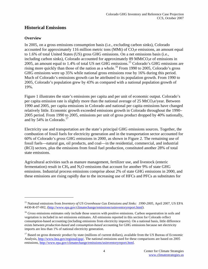
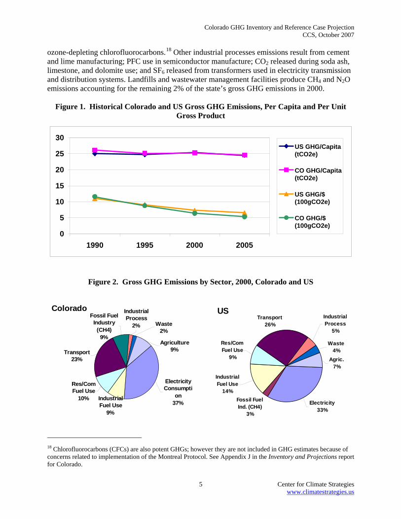
Historical Emissions Overview In 2005, on a gross emissions consumption basis (i.e., excluding carbon sinks), Colorado accounted for approximately 116 million metric tons (MMt) of CO2e emissions, an amount equal to 1.6% of total United States (US) gross GHG emissions. On a net emissions basis (i.e., including carbon sinks), Colorado accounted for approximately 89 MMtCO2e of emissions in 2005, an amount equal to 1.4% of total US net GHG emissions.15 Colorado’s GHG emissions are rising more quickly than those of the nation as a whole.16 From 1990 to 2005, Colorado’s gross GHG emissions were up 35% while national gross emissions rose by 16% during this period. Much of Colorado’s emissions growth can be attributed to its population growth. From 1990 to 2005, Colorado’s population grew by 43% as compared with a national population growth of 19%. Figure 1 illustrates the state’s emissions per capita and per unit of economic output. Colorado’s per capita emission rate is slightly more than the national average of 25 MtCO2e/year. Between 1990 and 2005, per capita emissions in Colorado and national per capita emissions have changed relatively little. Economic growth exceeded emissions growth in Colorado throughout the 1990–2005 period. From 1990 to 2005, emissions per unit of gross product dropped by 40% nationally, and by 54% in Colorado.17 Electricity use and transportation are the state’s principal GHG emissions sources. Together, the combustion of fossil fuels for electricity generation and in the transportation sector accounted for 60% of Colorado’s gross GHG emissions in 2000, as shown in Figure 2. The remaining use of fossil fuels—natural gas, oil products, and coal—in the residential, commercial, and industrial (RCI) sectors, plus the emissions from fossil fuel production, constituted another 28% of total state emissions. Agricultural activities such as manure management, fertilizer use, and livestock (enteric fermentation) result in CH4 and N2O emissions that account for another 9% of state GHG emissions. Industrial process emissions comprise about 2% of state GHG emissions in 2000, and these emissions are rising rapidly due to the increasing use of HFCs and PFCs as substitutes for
15 National emissions from Inventory of US Greenhouse Gas Emissions and Sinks: 1990-2005, April 2007, US EPA #430-R-07-002, (http://www.epa.gov/climatechange/emissions/usinventoryreport.html). 16 Gross emissions estimates only include those sources with positive emissions. Carbon sequestration in soils and vegetation is included in net emissions estimates. All emissions reported in this section for Colorado reflect consumption-based accounting (including emissions from electricity imports). On a national basis, little difference exists between production-based and consumption-based accounting for GHG emissions because net electricity imports are less than 1% of national electricity generation. 17 Based on gross domestic product by state (millions of current dollars), available from the US Bureau of Economic Analysis, http://www.bea.gov/regional/gsp/. The national emissions used for these comparisons are based on 2005 emissions, http://www.epa.gov/climatechange/emissions/usinventoryreport.html.
Colorado GHG Inventory and Reference Case Projection CCS, October 2007
5 Center for Climate Strategies www.climatestrategies.us
ozone-depleting chlorofluorocarbons.18 Other industrial processes emissions result from cement and lime manufacturing; PFC use in semiconductor manufacture; CO2 released during soda ash, limestone, and dolomite use; and SF6 released from transformers used in electricity transmission and distribution systems. Landfills and wastewater management facilities produce CH4 and N2O emissions accounting for the remaining 2% of the state’s gross GHG emissions in 2000.
Figure 1. Historical Colorado and US Gross GHG Emissions, Per Capita and Per Unit Gross Product
0
5
10
15
20
25
30
1990 1995 2000 2005
US GHG/Capita(tCO2e)
CO GHG/Capita(tCO2e)
US GHG/$(100gCO2e)
CO GHG/$(100gCO2e)
Figure 2. Gross GHG Emissions by Sector, 2000, Colorado and US
Colorado
Agriculture9%
Industrial Process
2%
Industrial Fuel Use
9%
Waste 2%
Transport23%
Fossil Fuel Industry
(CH4)9%
Res/Com Fuel Use
10%
Electricity Consumpti
on37%
Agric.7%
Electricity33%
Waste4%
Industrial Fuel Use
14%Fossil Fuel Ind. (CH4)
3%
Res/Com Fuel Use
9%
Industrial Process
5%
Transport26%
US
18 Chlorofluorocarbons (CFCs) are also potent GHGs; however they are not included in GHG estimates because of concerns related to implementation of the Montreal Protocol. See Appendix J in the Inventory and Projections report for Colorado.
Colorado GHG Inventory and Reference Case Projection CCS, October 2007
6 Center for Climate Strategies www.climatestrategies.us
Based on data from the early 1980s through 2004, Colorado’s forests are estimated to be net sinks, accounting for –24.7 MMtCO2 of GHG emissions (the negative value indicates a net sequestration of CO2 from the atmosphere). Also, agricultural soils are estimated to sequester an additional –2.0 MMtCO2. With these GHG sinks, Colorado’s net emissions were 59.4 MMtCO2 in 1990. Due to a lack of information to estimate future trends, these sinks were estimated to remain constant throughout the forecast period from 2005 through 2020. Thus, with the increase in GHG emission sources, by 2020, the net emissions in Colorado are estimated to increase to about 121 MMtCO2e. A Closer Look at the Two Major Sources: Electricity and Transportation As shown in Figure 2, electricity consumption accounted for about 37% of Colorado’s gross GHG emissions in 2000 (about 40.9 MMtCO2e), which was higher than the national average share of emissions from electricity consumption (33%).19 The GHG emissions associated with Colorado’s electricity sector increased by 8.2 MMtCO2e between 1990 and 2000, accounting for about 35% of the state’s net growth in gross GHG emissions in this time period. It is important to note that these GHG emissions estimates reflect the GHG emissions associated with the electricity sources used to meet Colorado demands, corresponding to a consumption-based approach to emissions accounting. Another way to look at electricity emissions is to consider the GHG emissions produced by electricity generation facilities in the state (see “Approach” section below). While we estimate emissions associated with both electricity production and consumption, unless otherwise indicated, tables, figures, and totals in this report reflect electricity consumption-based emissions. In 2000, emissions associated with Colorado’s electricity consumption (40.9 MMtCO2e) were slightly higher than those associated with electricity production (38.7 MMtCO2e) see Table 1. The higher level for consumption-based emissions reflects GHG emissions associated with net imports of electricity to meet the state’s electricity demand.20 The consumption-based approach can better reflect the emissions (and emissions reductions) associated with activities occurring in the state, particularly with respect to electricity use (and efficiency improvements), and is particularly useful for policy-making. Under this approach, emissions associated with electricity imported from other states would need to be covered in those states’ accounts in order to avoid double-counting or exclusions. (Indeed, Arizona, California, Oregon, New Mexico, and Washington are currently considering such an approach.) Like electricity emissions, GHG emissions from transportation fuel use have risen steadily from 1990 through 2000 at an average rate of slightly under 3% annually. In 2002, onroad gasoline vehicles accounted for about 66% of transportation GHG emissions. Onroad diesel vehicles accounted for another 20% of emissions, and air travel for roughly 11%. Rail, marine gasoline, and other sources (natural gas- and liquefied petroleum gas- (LPG-) fueled-vehicles and used in transport applications) accounted for the remaining 2% of transportation emissions. As the result 19 For the US as a whole, there is relatively little difference between the emissions from electricity use and emissions from electricity production, as the US imports only about 1% of its electricity, and exports far less. Colorado’s situation is different, since it is a net electricity importer. 20 Estimating the emissions associated with electricity use requires an understanding of the electricity sources (both in-state and out-of-state) used by utilities to meet consumer demand. The current estimate reflects some very simple assumptions, as described in Appendix A.
Colorado GHG Inventory and Reference Case Projection CCS, October 2007
7 Center for Climate Strategies www.climatestrategies.us
of Colorado’s population and economic growth and an increase in total vehicle miles traveled (VMT) during the 1990s, onroad gasoline use grew 32% between 1990 and 2002. Meanwhile, onroad diesel use rose 151% during that period, suggesting an even more rapid growth in freight movement within or across the state. Aviation fuel use grew by 16% from 1990 to 2002. Reference Case Projections Relying on a variety of sources for projections of electricity and fuel use, as noted below and in the Appendices, a simple reference case projection of GHG emissions through 2020 was developed. Table 2 shows key annual growth rates used to project emissions for Colorado and provides historical growth rates for comparison. As illustrated in Figure 3 and shown numerically in Table 1, under the reference case projections, Colorado gross GHG emissions continue to grow steadily, climbing to approximately 148 MMtCO2e by 2020, 71% above 1990 levels. Overall, the average annual projected rate of emissions growth in Colorado is 1.6% per year from 2005 to 2020. Demand for electricity is projected to be the largest contributor to future emissions growth accounting for about 36% of total gross GHG emissions in 2020, followed by emissions associated with transportation (25%), RCI fossil fuel use (19%), and fossil fuel production (8%) (see Figure 4).
Table 2. Key Annual Growth Rates for Colorado, Historical and Projected
1990-2005 2005-2020 Sources
Population* 2.4% 1.8% Colorado State Demography Office
Employment* Goods Services
1.0% 2.8%
2.7% 2.8%
Colorado Department of Labor and Employment website, based on analysis by the US Bureau of Labor Statistics.
Electricity Sales 3.0% 2.1% US DOE Energy Information Administration (EIA) data for 1990-2004 (3.0% growth is mix of increased residential and commercial electricity sales countered by a decrease in industrial sales). The growth rate for 2005-2020 is based on electricity sales forecasts developed for the energy supply sector, and includes state legislation passed in 2007 establishing new requirements for Colorado’s renewable portfolio standard and for demand-side management programs (see Appendix A).
Vehicle Miles Traveled
3.1% 2.1% Federal Highway Administration, Highway Statistic; Metropolitan Planning Organizations and CDPHE
* For the RCI fuel consumption sectors, population and employment projections for Colorado were used together with US DOE EIA’s Annual Energy Outlook 2006 (AEO2006) projections of changes in fuel use for the EIA’s Mountain region on a per capita basis for the residential sector, and on a per employee basis for the commercial and industrial sectors. For instance, growth in Colorado’s residential natural gas use is calculated as the Colorado population growth times the change in per capita natural gas use for the Mountain region.
Colorado GHG Inventory and Reference Case Projection CCS, October 2007
8 Center for Climate Strategies www.climatestrategies.us
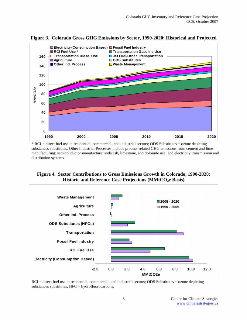
Figure 3. Colorado Gross GHG Emissions by Sector, 1990-2020: Historical and Projected
0
20
40
60
80
100
120
140
160
1990 2000 2005 2010 2015 2020
MM
tCO
2e
Electricity (Consumption Based) Fossil Fuel IndustryRCI Fuel Use * Transportation Gasoline UseTransportation Diesel Use Jet Fuel/Other TransportationAgriculture ODS SubstitutesOther Ind. Process Waste Management
* RCI = direct fuel use in residential, commercial, and industrial sectors; ODS Substitutes = ozone depleting substances substitutes. Other Industrial Processes include process-related GHG emissions from cement and lime manufacturing; semiconductor manufacture; soda ash, limestone, and dolomite use; and electricity transmission and distribution systems.
Figure 4. Sector Contributions to Gross Emissions Growth in Colorado, 1990-2020: Historic and Reference Case Projections (MMtCO2e Basis)
-2.0 0.0 2.0 4.0 6.0 8.0 10.0 12.0
Electricity (Consumption Based)
RCI Fuel Use
Fossil Fuel Industry
Transportation
ODS Substitutes (HFCs)
Other Ind. Process
Agriculture
Waste Management
MMtCO2e
2005 - 20201990 - 2005
RCI = direct fuel use in residential, commercial, and industrial sectors; ODS Substitutes = ozone depleting substances substitutes; HFC = hydrofluorocarbons.

Colorado GHG Inventory and Reference Case Projection CCS, October 2007
9 Center for Climate Strategies www.climatestrategies.us
CAP Revisions The following identifies the revisions that the CAP made to the inventory and reference case projections thus explaining the differences between the information presented in this report and the preliminary information presented in the January 2007 report:
• Energy Supply: Lowered emissions to account for changes in reference case assumptions associated with Colorado’s Renewable Portfolio Standard (RPS), which was amended upward in 2007 by the state legislature’s passage of House Bill (HB) 07-1281 (Renewable Energy Standards):
• Investor-Owned Utilities (IOUs) to provide 20% renewable energy by 2020 • Non-IOUs (e.g., municipal utilities and rural electric cooperatives) to provide 10%
renewable energy by 2020 • Incentives for in-state generation, community-based projects, and solar energy
• RCI: Reduced energy consumption in the reference case projections associated with the passage of HB 07-1146 (Energy Conservation Building Codes) in 2007. This bill requires local governments who have building codes to adopt energy efficiency codes for certain buildings.21 Reduction in emissions is accounted for under the RPS adjustment to avoid double counting of emission reductions.
• RCI: Reduced energy consumption in the reference case projections associated with the passage of HB 07-1037 (legislation recently passed requiring that public electric and gas utilities implement demand-side management programs) 22 and Xcel’s demand side management commitments under a recent legal settlement, both of which have the effect of limiting demand growth relative to what it would have been in the absence of these factors.23
• Waste Management: Revisions to municipal solid waste (MSW) to reflect revisions the US Environmental Protection Agency made to the methods for calculating emissions in US EPA’s State Greenhouse Gas Inventory Tool (SGIT; i.e., change was from use of regression equations to LANDGEM model equation):
• 1990 emissions decrease from 1.6 to 0.8 MMtCO2e • 2020 emissions decrease from 5.7 to 2.7 MMtCO2e
• Forestry: Removed forest soil organic carbon emissions sink as recommended by the United States Forest Service (USFS). Relative to the January 2007 report, this change removed 7.1 MMtCO2e of emissions from the forest sink pool for 1990 through 2020.
21 http://www.statebillinfo.com/sbi/index.cfm?fuseaction=Bills.View&billnum=HB07-1146. 22 http://www.statebillinfo.com/sbi/index.cfm?fuseaction=Bills.View&billnum=HB07-1037. 23 Comprehensive Settlement Agreement, docket 04A-214E, 04A-215E, and 04A-216E, issued December 3, 2004, available at http://www.xcelenergy.com/docs/corpcomm/SettlementAgreementFinalDraftclean20041203.pdf.
Colorado GHG Inventory and Reference Case Projection CCS, October 2007
10 Center for Climate Strategies www.climatestrategies.us
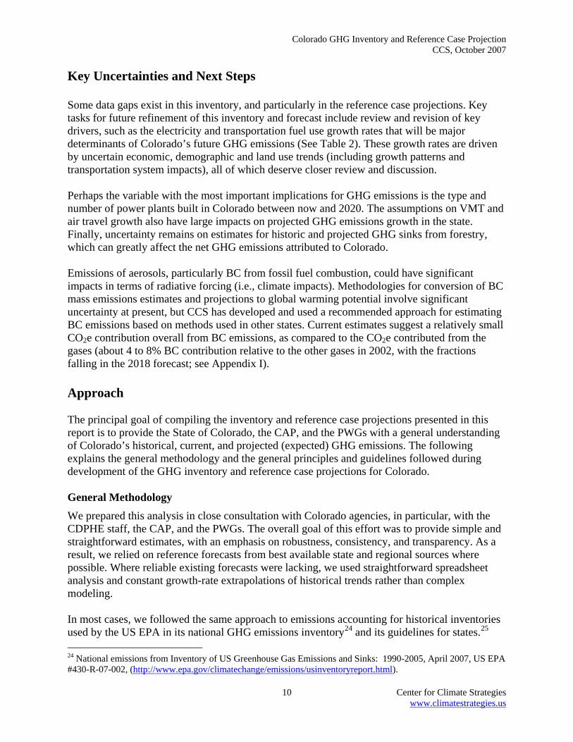
Key Uncertainties and Next Steps Some data gaps exist in this inventory, and particularly in the reference case projections. Key tasks for future refinement of this inventory and forecast include review and revision of key drivers, such as the electricity and transportation fuel use growth rates that will be major determinants of Colorado’s future GHG emissions (See Table 2). These growth rates are driven by uncertain economic, demographic and land use trends (including growth patterns and transportation system impacts), all of which deserve closer review and discussion. Perhaps the variable with the most important implications for GHG emissions is the type and number of power plants built in Colorado between now and 2020. The assumptions on VMT and air travel growth also have large impacts on projected GHG emissions growth in the state. Finally, uncertainty remains on estimates for historic and projected GHG sinks from forestry, which can greatly affect the net GHG emissions attributed to Colorado. Emissions of aerosols, particularly BC from fossil fuel combustion, could have significant impacts in terms of radiative forcing (i.e., climate impacts). Methodologies for conversion of BC mass emissions estimates and projections to global warming potential involve significant uncertainty at present, but CCS has developed and used a recommended approach for estimating BC emissions based on methods used in other states. Current estimates suggest a relatively small CO2e contribution overall from BC emissions, as compared to the CO2e contributed from the gases (about 4 to 8% BC contribution relative to the other gases in 2002, with the fractions falling in the 2018 forecast; see Appendix I). Approach The principal goal of compiling the inventory and reference case projections presented in this report is to provide the State of Colorado, the CAP, and the PWGs with a general understanding of Colorado’s historical, current, and projected (expected) GHG emissions. The following explains the general methodology and the general principles and guidelines followed during development of the GHG inventory and reference case projections for Colorado. General Methodology We prepared this analysis in close consultation with Colorado agencies, in particular, with the CDPHE staff, the CAP, and the PWGs. The overall goal of this effort was to provide simple and straightforward estimates, with an emphasis on robustness, consistency, and transparency. As a result, we relied on reference forecasts from best available state and regional sources where possible. Where reliable existing forecasts were lacking, we used straightforward spreadsheet analysis and constant growth-rate extrapolations of historical trends rather than complex modeling. In most cases, we followed the same approach to emissions accounting for historical inventories used by the US EPA in its national GHG emissions inventory24 and its guidelines for states.25 24 National emissions from Inventory of US Greenhouse Gas Emissions and Sinks: 1990-2005, April 2007, US EPA #430-R-07-002, (http://www.epa.gov/climatechange/emissions/usinventoryreport.html).
Colorado GHG Inventory and Reference Case Projection CCS, October 2007
11 Center for Climate Strategies www.climatestrategies.us
These inventory guidelines were developed based on the guidelines from the IPCC, the international organization responsible for developing coordinated methods for national GHG inventories.26 The inventory methods provide flexibility to account for local conditions. The key sources of activity and projection data used are shown in Table 3. Table 3 also provides the descriptions of the data provided by each source and the uses of each data set in this analysis. General Principles and Guidelines A key part of this effort involves the establishment and use of a set of generally accepted accounting principles for evaluation of historical and projected GHG emissions, as follows:
• Transparency: We reported data sources, methods, and key assumptions to allow open
review and opportunities for additional revisions by the CAP and PWGs.
• Consistency: To the extent possible, the inventory and projections will be designed to be externally consistent with current or likely future systems for state and national GHG emission reporting. We used US EPA tools for state inventories and projections as a starting point. These initial estimates were then augmented and/or revised as needed to conform with state-based inventory and base-case projection needs. For consistency in making reference case projections27, we define reference case actions for the purposes of projections as those currently in place or reasonably expected over the time period of analysis.
• Comprehensive Coverage of Gases, Sectors, State Activities, and Time Periods. This
analysis aimed to comprehensively cover GHG emissions associated with activities in Colorado. It covers all six GHGs covered by US and other national inventories: CO2, CH4, N2O, SF6, HFCs, PFCs, and BC. The inventory estimates are for the year 1990, with subsequent years included up to most recently available data (typically 2002 to 2005), with projections to 2010 and 2020.
• Priority of Significant Emissions Sources: In general, activities with relatively small
emissions levels were not reported with the same level of detail as other activities.
• Priority of Existing State and Local Data Sources: In gathering data and in cases where data sources conflicted, we placed highest priority on local and state data and analyses, followed by regional sources, with national data or simplified assumptions such as constant linear extrapolation of trends used as defaults where necessary.
• Use of Consumption-Based Emissions Estimates: To the extent possible, we estimated
emissions that are caused by activities that occur in Colorado. For example, we reported emissions associated with the electricity consumed in Colorado. The rationale for this
25 http://yosemite.epa.gov/oar/globalwarming.nsf/content/EmissionsStateInventoryGuidance.html. 26 http://www.ipcc-nggip.iges.or.jp/public/gl/invs1.htm. 27 “Reference case” is similar to the term “base year” used in criteria pollutant inventories. However, it also generally contains both a most current year estimate (e.g., 2002 or 2005), as well as estimates for historical years (e.g., 1990, 2000). Projections from this reference case are made to future years based on business-as-usual assumptions of future year source activity.
Colorado GHG Inventory and Reference Case Projection CCS, October 2007
12 Center for Climate Strategies www.climatestrategies.us
method of reporting is that it can more accurately reflect the impact of state-based policy strategies such as energy efficiency on overall GHG emissions, and it resolves double-counting and exclusion problems with multi-emissions issues. This approach can differ from how inventories are compiled, for example, on an in-state production basis, in particular for electricity.
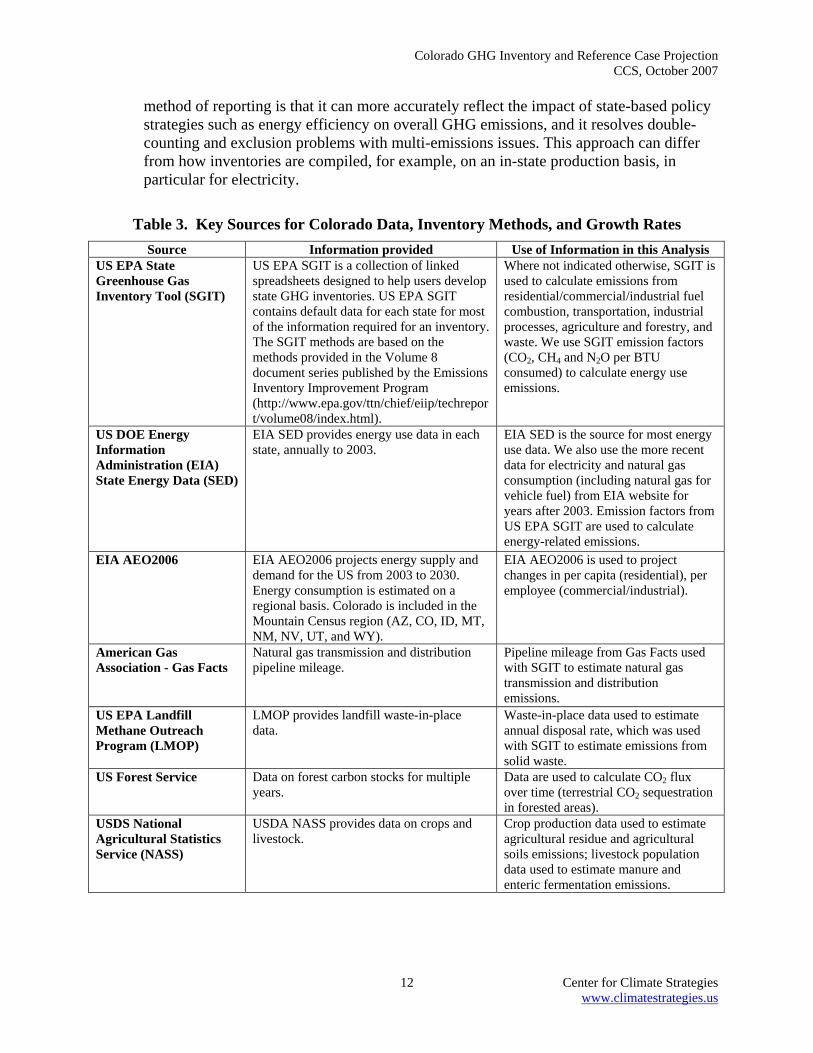
Table 3. Key Sources for Colorado Data, Inventory Methods, and Growth Rates Source Information provided Use of Information in this Analysis
US EPA State Greenhouse Gas Inventory Tool (SGIT)
US EPA SGIT is a collection of linked spreadsheets designed to help users develop state GHG inventories. US EPA SGIT contains default data for each state for most of the information required for an inventory. The SGIT methods are based on the methods provided in the Volume 8 document series published by the Emissions Inventory Improvement Program (http://www.epa.gov/ttn/chief/eiip/techreport/volume08/index.html).
Where not indicated otherwise, SGIT is used to calculate emissions from residential/commercial/industrial fuel combustion, transportation, industrial processes, agriculture and forestry, and waste. We use SGIT emission factors (CO2, CH4 and N2O per BTU consumed) to calculate energy use emissions.
US DOE Energy Information Administration (EIA) State Energy Data (SED)
EIA SED provides energy use data in each state, annually to 2003.
EIA SED is the source for most energy use data. We also use the more recent data for electricity and natural gas consumption (including natural gas for vehicle fuel) from EIA website for years after 2003. Emission factors from US EPA SGIT are used to calculate energy-related emissions.
EIA AEO2006
EIA AEO2006 projects energy supply and demand for the US from 2003 to 2030. Energy consumption is estimated on a regional basis. Colorado is included in the Mountain Census region (AZ, CO, ID, MT, NM, NV, UT, and WY).
EIA AEO2006 is used to project changes in per capita (residential), per employee (commercial/industrial).
American Gas Association - Gas Facts
Natural gas transmission and distribution pipeline mileage.
Pipeline mileage from Gas Facts used with SGIT to estimate natural gas transmission and distribution emissions.
US EPA Landfill Methane Outreach Program (LMOP)
LMOP provides landfill waste-in-place data.
Waste-in-place data used to estimate annual disposal rate, which was used with SGIT to estimate emissions from solid waste.
US Forest Service Data on forest carbon stocks for multiple years.
Data are used to calculate CO2 flux over time (terrestrial CO2 sequestration in forested areas).
USDS National Agricultural Statistics Service (NASS)
USDA NASS provides data on crops and livestock.
Crop production data used to estimate agricultural residue and agricultural soils emissions; livestock population data used to estimate manure and enteric fermentation emissions.
Colorado GHG Inventory and Reference Case Projection CCS, October 2007
13 Center for Climate Strategies www.climatestrategies.us
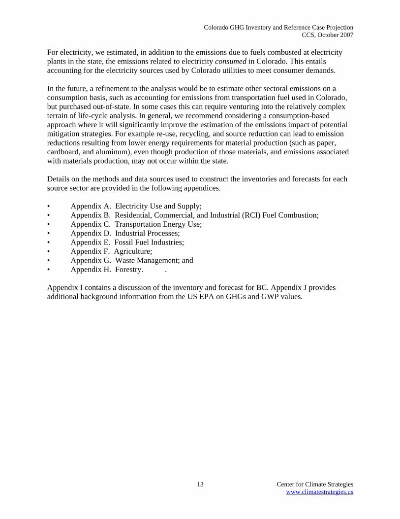
For electricity, we estimated, in addition to the emissions due to fuels combusted at electricity plants in the state, the emissions related to electricity consumed in Colorado. This entails accounting for the electricity sources used by Colorado utilities to meet consumer demands. In the future, a refinement to the analysis would be to estimate other sectoral emissions on a consumption basis, such as accounting for emissions from transportation fuel used in Colorado, but purchased out-of-state. In some cases this can require venturing into the relatively complex terrain of life-cycle analysis. In general, we recommend considering a consumption-based approach where it will significantly improve the estimation of the emissions impact of potential mitigation strategies. For example re-use, recycling, and source reduction can lead to emission reductions resulting from lower energy requirements for material production (such as paper, cardboard, and aluminum), even though production of those materials, and emissions associated with materials production, may not occur within the state. Details on the methods and data sources used to construct the inventories and forecasts for each source sector are provided in the following appendices. • Appendix A. Electricity Use and Supply; • Appendix B. Residential, Commercial, and Industrial (RCI) Fuel Combustion; • Appendix C. Transportation Energy Use; • Appendix D. Industrial Processes; • Appendix E. Fossil Fuel Industries; • Appendix F. Agriculture; • Appendix G. Waste Management; and • Appendix H. Forestry. . Appendix I contains a discussion of the inventory and forecast for BC. Appendix J provides additional background information from the US EPA on GHGs and GWP values.

Colorado GHG Inventory and Reference Case Projection CCS, October 2007
A-1 Center for Climate Strategies www.climatestrategies.us
Appendix A. Electricity Use and Supply Overview Colorado’s electric sector has experienced strong growth in the last 15 years, mostly driven by population and economic growth in the state. These drivers, and the state’s electric sector, appear likely to experience continued growth for some time. Greenhouse gas (GHG) emissions associated with electricity production and consumption accounted for about 36% of Colorado’s gross GHG emissions in 2005. As noted in the main report, one of the key questions for the state to consider is how to treat GHG emissions that result from generation of electricity that is produced outside Colorado to meet electricity needs in the state. In other words, should the state consider the GHG emissions associated with the state’s electricity consumption, with its electricity production, or with some combination of the two? This appendix describes GHG emissions from Colorado’s electricity sector in terms of emissions from both electricity consumption and production, including the assumptions used to develop the reference case projections. It then describes Colorado’s electricity trade and potential approaches for allocating GHG emissions for the purpose of determining the state’s inventory and reference case projections. In addition, as discussed at the end of this appendix, the reference case projections were updated to reflect recent legislation that increased requirements for renewable fuels in Colorado’s Renewable Portfolio Standard (RPS), which was amended by the Colorado State Legislature in 2007 by House Bill (HB) 07-1281 (Renewable Energy Standards), and requirements for demand-side management programs (DSM). Finally, key assumptions and results are summarized. Electricity Consumption At about 10,000 kilowatt-hour (kWh) per capita (2004 data), Colorado has relatively low electricity consumption per capita. By way of comparison, the annual per capita consumption for the US was about 12,000 kWh/capita.28 Figure A1 shows Colorado’s rank compared to other western states from 1960-1999; while showing stronger increases during this time period than most states, Colorado’s per capita consumption has been relatively low (2nd lowest, effectively tied with Utah and New Mexico for much of 1985 to 1999). Many factors influence a state’s per capita electricity consumption, including the impact of weather on demand for cooling and heating, the size and type of industries in the state, and the type and efficiency of equipment in use in the residential, commercial and industrial sectors.
28 Census bureau for U.S. population, Energy Information Administration for electricity sales.

Colorado GHG Inventory and Reference Case Projection CCS, October 2007
A-2 Center for Climate Strategies www.climatestrategies.us
Figure A1. Electricity Consumption per capita in Western States, 1960-1999
Source: Northwest Power Council, 5th Power Plan, Appendix A Note: MWhr is Megawatt-hours.
As shown in Figure A2, electricity sales in the Colorado have generally increased steadily from 1990 through 2004. Overall, total electricity consumption increased at an average annual rate of 3% from 1990 to 2004, which can be compared with population growth at a rate of 2.5% per year and gross state product increases averaging of 4.3%/yr over the same period.29 During this period, residential sector consumption grew by an average of 3.4% per year, commercial sector use grew by 2.2% per year, and industrial sector consumption increased at 4.2% per year. The industrial sector electricity sales increases in Colorado have not been uniform over this period – total industrial sector sales increased by 37% from 1993 to 1994, then by less than 4% from 1994 through 2000.30
29 Populations from Colorado’s Databook. Gross State Production from Bureau of Economic analysis. Available as http://bea.gov/bea/newsrelarchive/2006/gsp1006.xls 30 CCS checked this value with EIA who were unable to determine the exact source of the increase. The data are reported directly by utilities to EIA.

Colorado GHG Inventory and Reference Case Projection CCS, October 2007
A-3 Center for Climate Strategies www.climatestrategies.us
Figure A2. Electricity Consumption by Sector in Colorado, 1990-200431
0
5,000
10,000
15,000
20,000
25,000
1990
1991
1992
1993
1994
1995
1996
1997
1998
1999
2000
2001
2002
2003
2004
Gig
awat
t-hou
rs (G
Wh)
ResidentialCommercialIndustrial
Source: EIA State Energy Data (SED) (1990-2002) and EIA Electric Power Annual (2003-2004)
The Colorado Energy Forum recently released a report, Colorado’s Electricity Future.32 This report provides projections for electricity sales in Colorado, excluding the impacts of any additional investments in energy efficiency programs. These projections were developed by RW Beck by compiling forecasts from the largest utility providers in Colorado and extrapolating these forecasts to smaller electricity suppliers in similar regions. The RW Beck analysis included a base case forecast, plus high- and low-case sensitivities. The base case projection was used for the current analysis. Table A1 reports historic and projected annual average growth rates for electricity use in Colorado.
31 Note that from 1990-2002, the US Department of Energy (US DOE) Energy Information Administration (EIA) data includes a category referred to as “other,” which included lighting for public buildings, streets, and highways, interdepartmental sales, and other sales to public authorities, agricultural and irrigation sales where separately identified, electrified rail and various urban transit systems (such as automated guideway, trolley, and cable systems). To report total electricity in Figure A2, the sales from the “other” category are included with commercial sector sales. The decision to include sales listed as “other” with commercial rather than the residential or industrial sector sales data was based on a comparison of the trends of electricity sales from 2000-2002 with sales are categorized in 2003 EIA data. 32 Colorado’s Electricity Future: An Analysis by the Colorado Energy Forum Incorporating Three Separate Reports by: R.W. Beck Inc., Schmitz Consulting LLC, and The Colorado School of Mines (September 2006)
Colorado GHG Inventory and Reference Case Projection CCS, October 2007
A-4 Center for Climate Strategies www.climatestrategies.us
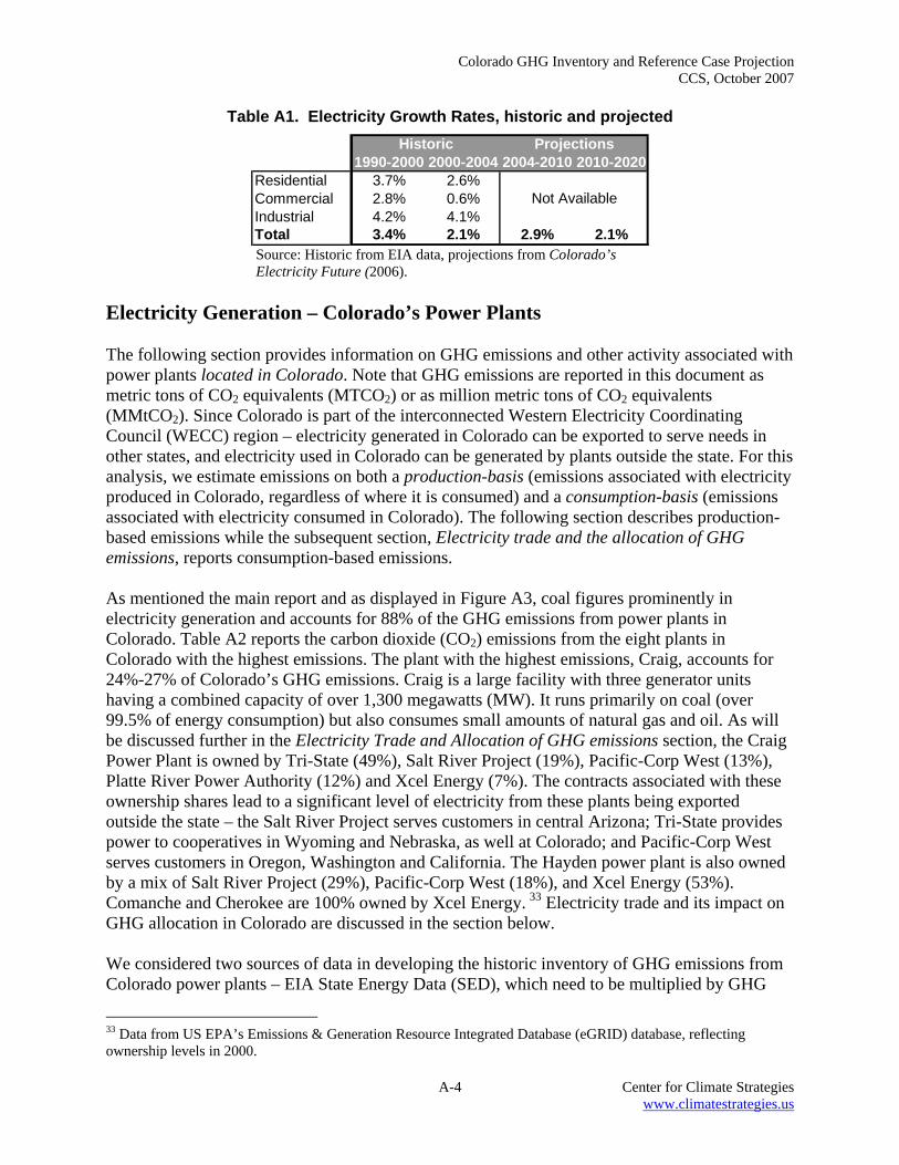
Table A1. Electricity Growth Rates, historic and projected
1990-2000 2000-2004 2004-2010 2010-2020Residential 3.7% 2.6%Commercial 2.8% 0.6%Industrial 4.2% 4.1%Total 3.4% 2.1% 2.9% 2.1%
Historic Projections
Not Available
Source: Historic from EIA data, projections from Colorado’s Electricity Future (2006).
Electricity Generation – Colorado’s Power Plants The following section provides information on GHG emissions and other activity associated with power plants located in Colorado. Note that GHG emissions are reported in this document as metric tons of CO2 equivalents (MTCO2) or as million metric tons of CO2 equivalents (MMtCO2). Since Colorado is part of the interconnected Western Electricity Coordinating Council (WECC) region – electricity generated in Colorado can be exported to serve needs in other states, and electricity used in Colorado can be generated by plants outside the state. For this analysis, we estimate emissions on both a production-basis (emissions associated with electricity produced in Colorado, regardless of where it is consumed) and a consumption-basis (emissions associated with electricity consumed in Colorado). The following section describes production-based emissions while the subsequent section, Electricity trade and the allocation of GHG emissions, reports consumption-based emissions. As mentioned the main report and as displayed in Figure A3, coal figures prominently in electricity generation and accounts for 88% of the GHG emissions from power plants in Colorado. Table A2 reports the carbon dioxide (CO2) emissions from the eight plants in Colorado with the highest emissions. The plant with the highest emissions, Craig, accounts for 24%-27% of Colorado’s GHG emissions. Craig is a large facility with three generator units having a combined capacity of over 1,300 megawatts (MW). It runs primarily on coal (over 99.5% of energy consumption) but also consumes small amounts of natural gas and oil. As will be discussed further in the Electricity Trade and Allocation of GHG emissions section, the Craig Power Plant is owned by Tri-State (49%), Salt River Project (19%), Pacific-Corp West (13%), Platte River Power Authority (12%) and Xcel Energy (7%). The contracts associated with these ownership shares lead to a significant level of electricity from these plants being exported outside the state – the Salt River Project serves customers in central Arizona; Tri-State provides power to cooperatives in Wyoming and Nebraska, as well at Colorado; and Pacific-Corp West serves customers in Oregon, Washington and California. The Hayden power plant is also owned by a mix of Salt River Project (29%), Pacific-Corp West (18%), and Xcel Energy (53%). Comanche and Cherokee are 100% owned by Xcel Energy. 33 Electricity trade and its impact on GHG allocation in Colorado are discussed in the section below. We considered two sources of data in developing the historic inventory of GHG emissions from Colorado power plants – EIA State Energy Data (SED), which need to be multiplied by GHG
33 Data from US EPA’s Emissions & Generation Resource Integrated Database (eGRID) database, reflecting ownership levels in 2000.

Colorado GHG Inventory and Reference Case Projection CCS, October 2007
A-5 Center for Climate Strategies www.climatestrategies.us
emission factors for each type of fuel consumed, and United States Environmental Protection Agency (US EPA) data on CO2 emissions by power plant. For total electric sector GHG emissions, we used the EIA’s State Energy Data (SED) rather than US EPA data because of the comprehensiveness of the EIA-based data. The US EPA data are limited to plants over 25 MW and include only CO2 emissions (US EPA does not collect data on methane (CH4) or nitrous oxide (N2O) emissions). Through discussions with staff at the US EPA we also learned that US EPA data tend to be conservative (that is, overestimate emissions) because the data are reported as part of a regulatory program, and that during early years of the data collection program, missing data points were sometimes assigned a large value as a placeholder. However, the US EPA provides easily accessible data for each power plant (over 25 MW), which would be much more difficult to extract from EIA data, and the CO2 emissions from the two sources differ by less than 2% in most years. Based on this information, we chose to report information from both data sources, but rely on the EIA data for the inventory values. For total GHG emissions from electricity production in Colorado, we applied State Greenhouse Gas Inventory Tool (SGIT) emission factors34 to EIA’s SED. For CO2 emissions from individual plants, we used the EPA database.
Table A2. CO2 Emissions from Individual Colorado Power Plants, 2000-2005 (Million metric tons CO2) 2000 2001 2002 2003 2004 2005Cherokee 4.9 4.8 4.3 5.0 4.9 5.2Comanche 4.4 4.7 5.2 5.4 4.8 4.8Craig 9.5 9.7 9.7 9.7 10.4 10.5Hayden 3.6 3.8 4.0 3.6 3.8 4.1Martin Drake 2.0 2.1 2.0 2.1 1.8 2.2Pawnee 4.3 4.8 3.6 4.2 3.8 3.2Rawhide Energy Station 2.2 2.4 2.3 2.5 2.5 2.1Ray D Nixon 1.6 1.7 1.7 1.7 1.8 1.6Other Plants 6.0 6.8 6.7 5.4 5.5 6.0
Total CO2 emissions 38.5 40.7 39.5 39.6 39.3 39.6 Source: US EPA Clean Air Markets database for named plants (http://cfpub.epa.gov/index.cfm). Total emissions calculated from fuel use data provided by SED (EIA). Note: The emissions reported in the above table are CO2 only. CH4 and N2O emissions were not included in the power plant data available from the US EPA.
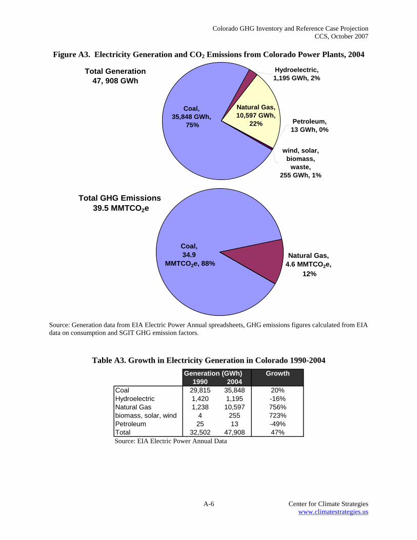
Table A3 shows the growth in generation by fuel type for all power plants in Colorado between 1990 and 2004. Overall generation grew by 47% over the 15 years, while electricity consumption grew by 52%. Natural gas-fired generation has been particularly strong, increasing by more than 8-fold from 1994 through 2004. Renewable generation (biomass, solar and wind) grew by a similar relative amount over the time period, but as of 2004 these resources accounted for only 0.5% of total generation. Coal generation grew more slowly but remains the dominant source of electricity in the state. Imports grew from an estimated 1,500 Gigawatt-hour (GWh) (4.6% of state generation) in 1990 to 3,500 GWh (7.6% of state generation) in 2004.
34 SGIT http://www.epa.gov/climatechange/emissions/state_guidance.html, National GHG inventory http://www.epa.gov/climatechange/emissions/usinventoryreport.html
Colorado GHG Inventory and Reference Case Projection CCS, October 2007
A-6 Center for Climate Strategies www.climatestrategies.us
Figure A3. Electricity Generation and CO2 Emissions from Colorado Power Plants, 2004
Total Generation 47, 908 GWh
Petroleum, 13 GWh, 0%
wind, solar, biomass,
waste, 255 GWh, 1%
Natural Gas, 10,597 GWh,
22%
Hydroelectric, 1,195 GWh, 2%
Coal, 35,848 GWh,
75%
Total GHG Emissions 39.5 MMTCO2e
Natural Gas, 4.6 MMTCO2e,
12%
Coal, 34.9
MMTCO2e, 88%
Source: Generation data from EIA Electric Power Annual spreadsheets, GHG emissions figures calculated from EIA data on consumption and SGIT GHG emission factors.
Table A3. Growth in Electricity Generation in Colorado 1990-2004 Growth
1990 2004Coal 29,815 35,848 20%Hydroelectric 1,420 1,195 -16%Natural Gas 1,238 10,597 756%biomass, solar, wind 4 255 723%Petroleum 25 13 -49%Total 32,502 47,908 47%
Generation (GWh)
Source: EIA Electric Power Annual Data
Colorado GHG Inventory and Reference Case Projection CCS, October 2007
A-7 Center for Climate Strategies www.climatestrategies.us
Future Generation and Emissions Estimating future generation and GHG emissions from Colorado power plants requires estimation of new power plant additions and production levels from new and existing power plants. There are, of course, large uncertainties, especially related to the timing and nature of new power plant construction. The future mix of generating plants in Colorado remains uncertain, as the trends in type of new builds are influenced by many factors. Since 1982, new fossil-fueled plants in Colorado have been natural gas-fired; however, concerns about the cost and availability of natural gas seem to have led to a trend towards a more coal-dominated mix. Recent announcements by several utilities indicate that coal-fired units will dominate new power plant builds. Xcel Energy has started construction on the Pueblo unit, an expansion of the Comanche power plant. Additionally, according a recent Denver Post article, Xcel has proposed to build a separate new plant, which would be “the nation's first power plant that converts coal to clean-burning gas and captures carbon emissions - viewed as an environmental breakthrough that will change coal's image from a belching polluter to an abundant, clean and relatively affordable resource. The plant could cost from $500 million to $1 billion or more, with a possible construction start in 2009.”35
In 2004, Colorado became the first state in the country to have voters directly approve a RPS, rather than have it processed through a state’s legislature.36 Colorado voters approved Amendment 37 and the state has recently begun implementation. The RPS requires utilities with over 40,000 customers to generate (or purchase) a minimum amount of electricity from renewable sources. Colorado’s RPS requires minimum annual contributions of renewable electricity of 3% from 2007 through 2010, 6% from 2011 through 2014; and 10% by 2015 and thereafter. Of the electricity generated each year from renewable sources, at least 4% must come from solar electric technologies. At least one-half of this percentage must come from solar electric systems located on-site at customers’ facilities. Other eligible technologies include wind, geothermal heat, biomass facilities that burn nontoxic plants, landfill gas, animal waste, small hydroelectric, and hydrogen fuel cells. Energy generated in Colorado is favored; each kWh of renewable electricity generated in-state will be counted as 1.25 kWh for the purposes of meeting this standard. The RPS will likely spur additional new wind and solar projects in the state. Xcel Energy’s Spring Canyon wind farm came on-line in 2006, and three other wind plants have been proposed for Colorado. Xcel has also announced a project to build and operate an 8 MW solar central solar power plant in Alamosa, Colorado, that will house two technologies: concentrating photovoltaic (PV) and advanced flat-plate solar panel units. The plant is expected to be on-line at the end of 2007, pending regulatory approval, and will be the largest PV central solar station in the United States.37 Table A4 presents data on new and proposed plants in Colorado.
35 http://www.denverpost.com/business/ci_4421583 36 Database of State Incentives for Renewables and Efficiency http://www.dsireusa.org/library/includes/incentive2.cfm?Incentive_Code=CO24R&state=CO&CurrentPageID=1&RE=1&EE=1 37 http://www.renewableenergyaccess.com/rea/news/story?id=46072

Colorado GHG Inventory and Reference Case Projection CCS, October 2007
A-8 Center for Climate Strategies www.climatestrategies.us
Note that proposals for individual plants cover the period through 2010. Beyond this time period it is necessary to make assumptions about expected growth. Given the many factors affecting electricity-related emissions and a diversity of assumptions by stakeholders within the electricity sector, developing a “reference case” projection for the most likely development of Colorado’s electricity sector is particularly challenging. Therefore, to develop an initial projection, simple assumptions were made, relying to the extent possible on widely-reviewed and accepted modeling assessments.
Table A4. New and Proposed Power Plants in Colorado Plant Name Fuel Status Capacity Notes
generation EmissionsMW GWh MMTCO2e
Colorado Green wind On-line 2003 162 500 0 All power will be sold to Xcel Energy under a long term Power Purchase Agreement
Spring Canyon wind On-line 2006 60 190 0 All power will be sold to Xcel Energy under a long term Power Purchase Agreement
Solar plant in Alamosa, Colorado
solar Proposed - end of 2007 8 13 0
Xcel Energy selected an affiliate of SunEdison, LLC, to build, own and operate this plant, PSCo will purchase the power and renewable energy credits
Xcel Wind Plants wind Proposed -
end of 2007 775 1697 0
Xcel Energy announced its intent to acquire 775 MW of new wind, to be in service by end of 2007. Xcel signed contracts with FPL and Invenergy for 400 MW of capacity.
Blue Spruce Energy Center gas On-line 2003 280 255 0.16 Generation and Emissions from US EPA
Clean Air Database for 2005Rawhide
expansion-Unit D
gas On-line 2004 74 3 less than 0.005
Generation and Emissions from US EPA Clean Air Database for 2005
Rocky Montain Energy Center gas On-line 2004 478 3,261 1.32 Generation and Emissions from US EPA
Clean Air Database for 2005
Xcel Natural Gas Plants gas 2007/2012 608 for 2007
193 for 2012 1050 by 2012 0.54Plants reported in Xcel Bid Evaluation report, generation based on 15% capacity factor (peaking plants)
Lamar Expansion coal
Application Pending -
200837 259 0.22
Generation based on 0.80 capacity factor, GHG emissions based on heatrate of 9000 british thermal unit per kWh (BTU/kWh)
Comanche Expansion coal
Under Construction
- Oct 2009750 5,256 4.38
Generation based on 0.80 capacity factor, GHG emissions based on heatrate of 9000 BTU/kWh
Expected Annual
Wind and Solar Plants
Non-Renewable Plants
Sources: Colorado Green – E-mail from Tim Oleary, Shell Renewables, November 10, 2006
Spring Canyon – E-mail from Phil Stiles, InvEnergy, October 18, 2006 Solar Plant – Xcel Energy press release, capacity factor from Wiser and Bolinger powerpoint
presentation 2006, newrules.org Xcel Wind Plants – Xcel press release, http://www.xcelenergy.com/XLWEB/CDA/0,3080,1-1-
1_15531_26314-28906-0_0_0-0,00.html Blue Spruce, Rawhide, Rocky Mountain – Colorado’s Electricity Future Xcel Natural Gas – Xcel Bid Evaluation report Lamar and Comanche expansion – Colorado’s Electricity Future
The reference case projections are based on CCS’s review of the analyses discussed below and assume:
• Generation from plants in Colorado grows at 2.8% per year from 2006-2010 – this growth reflects the estimated generation from the new plants that came on-line in 2006 or

Colorado GHG Inventory and Reference Case Projection CCS, October 2007
A-9 Center for Climate Strategies www.climatestrategies.us
are under-construction in the state (as reported in Table A3 above) and additional renewable generation that is required to meet the RPS.
• Generation from plants in Colorado grows at 2.5% per year from 2010 to 2015 and 2.0% from 2015 to 2020. This reflects the generation growth rate for the Rocky Mountain region in EIA’s Annual Energy Outlook 2006 (AEO2006). These assumptions lead to about 4300 MW of new power plant capacity by 2020 (excluding Comanche expansion).
• Generation from existing non-hydro plants is based on holding generation at 2004 levels. Generation from existing hydro-electric plants is assumed to be 1,597 GWh per year, the average generation from the last ten years. New plants and changes to existing plants due to plant renovations and overhauls that result in higher capacity factors are counted as new generation.
• The RPS requirements are assumed to be met by Xcel Energy and Aquila, the state’s investor-owned utilities. From 2007 to 2010, three of the public utilities (Colorado Spring, Holy Cross and Fort Collins) are expected to meet the RPS minimum requirements. From 2011 onwards, Longmont is also assumed to meet the RPS requirements. These utilities are expected to meet the requirements through self-certification and are assumed to meet the total renewable requirements, but not necessarily the solar requirements.38 The 2 investor-owned utilities and the 4 “publics” are estimated to account for 65% of electricity sales.39 This analysis assumes that 95% of the renewables will be located in-state and will receive an additional 25% credit toward the RPS requirements.40
• New fossil fuel plants built between 2010 and 2020 will be a mix of 80% coal and 20% natural gas, based on the mix projected for the Rocky Mountain region of WECC in the AEO2006.
• Following the definition of reference case that CCS is using – i.e., based on existing or soon-to-be enacted policies – the projections for the electric sector assume that the state does not enact rules designed to limit GHG emissions.
Electricity Trade and Allocation of GHG Emissions Colorado is part of the interconnected WECC region - a vast and diverse area covering 1.8 million square miles and extending from Canada through Mexico, including all or portions of 14 western states. The inter-connected region allows electricity generators and consumers to buy and sell electricity across regions, taking advantage of the range of resources and markets. Electricity generated by any single plant enters the interconnected grid and may contribute to meeting demand throughout much of the region, depending on sufficient transmission capacity. Thus, it is challenging to define, first, which emissions should be allocated to Colorado, and secondly, to estimate these allocated emissions both historically and into the future. Some
38 Information on utility plans for meeting RPS based on personal communication, Richard Mignogna, Colorado Department of Regulatory Agencies, October 23, 2006. 39 Based on utility sales data in 2004, from EIA. 40 CCS assumptions, needs verification
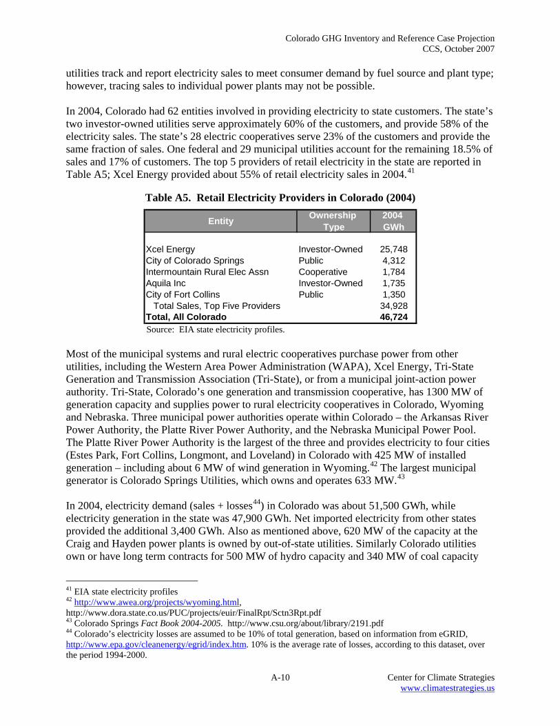
Colorado GHG Inventory and Reference Case Projection CCS, October 2007
A-10 Center for Climate Strategies www.climatestrategies.us
utilities track and report electricity sales to meet consumer demand by fuel source and plant type; however, tracing sales to individual power plants may not be possible. In 2004, Colorado had 62 entities involved in providing electricity to state customers. The state’s two investor-owned utilities serve approximately 60% of the customers, and provide 58% of the electricity sales. The state’s 28 electric cooperatives serve 23% of the customers and provide the same fraction of sales. One federal and 29 municipal utilities account for the remaining 18.5% of sales and 17% of customers. The top 5 providers of retail electricity in the state are reported in Table A5; Xcel Energy provided about 55% of retail electricity sales in 2004.41
Table A5. Retail Electricity Providers in Colorado (2004)
Entity Ownership Type
2004 GWh
Xcel Energy Investor-Owned 25,748City of Colorado Springs Public 4,312Intermountain Rural Elec Assn Cooperative 1,784Aquila Inc Investor-Owned 1,735City of Fort Collins Public 1,350 Total Sales, Top Five Providers 34,928Total, All Colorado 46,724 Source: EIA state electricity profiles.
Most of the municipal systems and rural electric cooperatives purchase power from other utilities, including the Western Area Power Administration (WAPA), Xcel Energy, Tri-State Generation and Transmission Association (Tri-State), or from a municipal joint-action power authority. Tri-State, Colorado’s one generation and transmission cooperative, has 1300 MW of generation capacity and supplies power to rural electricity cooperatives in Colorado, Wyoming and Nebraska. Three municipal power authorities operate within Colorado – the Arkansas River Power Authority, the Platte River Power Authority, and the Nebraska Municipal Power Pool. The Platte River Power Authority is the largest of the three and provides electricity to four cities (Estes Park, Fort Collins, Longmont, and Loveland) in Colorado with 425 MW of installed generation – including about 6 MW of wind generation in Wyoming.42 The largest municipal generator is Colorado Springs Utilities, which owns and operates 633 MW.43 In 2004, electricity demand (sales + losses44) in Colorado was about 51,500 GWh, while electricity generation in the state was 47,900 GWh. Net imported electricity from other states provided the additional 3,400 GWh. Also as mentioned above, 620 MW of the capacity at the Craig and Hayden power plants is owned by out-of-state utilities. Similarly Colorado utilities own or have long term contracts for 500 MW of hydro capacity and 340 MW of coal capacity
41 EIA state electricity profiles 42 http://www.awea.org/projects/wyoming.html, http://www.dora.state.co.us/PUC/projects/euir/FinalRpt/Sctn3Rpt.pdf 43 Colorado Springs Fact Book 2004-2005. http://www.csu.org/about/library/2191.pdf 44 Colorado’s electricity losses are assumed to be 10% of total generation, based on information from eGRID, http://www.epa.gov/cleanenergy/egrid/index.htm. 10% is the average rate of losses, according to this dataset, over the period 1994-2000.

Colorado GHG Inventory and Reference Case Projection CCS, October 2007
A-11 Center for Climate Strategies www.climatestrategies.us
from outside of the state. Thus, electricity trade counts for a significant portion of the electric power associated with Colorado. Since almost all states are part of regional trading grids, many states that have developed GHG inventories have grappled with the problem of how to account for electric sector emissions, when electricity flows across state borders. Several approaches have been developed to allocate GHG emissions from the electricity sector to individual states for inventories. In many ways the simplest approach is production-based – emissions from power plants within the state are included in the state’s inventory. The data for this estimate are publicly available and unambiguous. However, this approach is problematic for states that import or export significant amounts of electricity. Under a production-based approach, characteristics of Colorado electricity consumption would not be fully captured since only emissions from in-state generation would be considered. An alternative is to estimate consumption-based or load-based GHG emissions, corresponding to the emissions associated with electricity consumed in the state. The load-based approach is currently being considered by states that import significant amounts of electricity, such as California, Oregon, and Washington.45 By accounting for emissions from imported electricity, states can account for increases or decreases in fossil fuel consumed in power plants outside of the state, due to demand growth, efficiency programs, and other actions in the state. The difficulty with this approach is properly accounting for the emissions from imports and exports. Since the electricity flowing into or out of Colorado is a mix of all plants generating on the inter-connected grid, it is impossible to physically track the sources of the electrons. The approach taken in this initial inventory is a simplification of the consumption-based approach. This approach, which one could term “Net-Consumption-based,” estimates consumption-based emissions as in-state (production-based) emissions plus the emissions from the net imports. Emissions for net imports are calculated as net electricity imports (in GWh) multiplied by the average emission intensity for imports (in MtCO2e/GWh). Estimating the mix of electricity generation for the imports/export of a state is possible and several states are developing data collection approaches to do this. Washington State has developed regular fuel disclosure reporting.46 Colorado enacted legislation in 1999 that requires investor-owned utilities to disclose information on their fuel mix to retail customers.47 While this information would be helpful in estimating the fuel mix of electricity that is imported into Colorado by Xcel and Aquila, the information was not readily available.48 As a proxy for estimating the mix of historic 45 See for example, the reports of the Puget Sound Climate Protection Advisory Committee (http://www.pscleanair.org/specprog/globclim/), the Oregon Governor’s Advisory Group On Global Warming (http://egov.oregon.gov/ENERGY/GBLWRM/Strategy.shtml), and the California Climate Change Advisory Committee, Policy Options for Reducing Greenhouse Gas Emissions From Power Imports - Draft Consultant Report (http://www.energy.ca.gov/2005publications/CEC-600-2005-010/CEC-600-2005-010-D.PDF). 46 http://www.cted.wa.gov/site/539/default.aspx 47 Code of Colorado Regulations Rule 723-3-10(f) et seq. Information from Database of State Incentives for Renewables and Efficiency http://www.dsireusa.org/documents/Incentives/CO17R.htm 48 The fuel mix provided on Xcel Energy’s bills included a breakdown by fuel for electricity provided by plants in Colorado but did not include the fuel mix of imported electricity. Information on the legislation is listed at: http://www.dsireusa.org/library/includes/incentive2.cfm?Incentive_Code=CO17R&state=CO&CurrentPageID=1&RE=1&EE=0
Colorado GHG Inventory and Reference Case Projection CCS, October 2007
A-12 Center for Climate Strategies www.climatestrategies.us
and future GHG for Colorado’s electricity imports, emission intensities that reflect the regional fuel mix were used. Emissions from the Rocky Mountain region of the WECC (excluding Colorado’s emissions) were used to calculate GHG emission intensity for imports, with estimates of future Rocky Mountain emissions provided by the AEO2006. These regional emission factors were 0.61 MtCO2e/MWh in 2004, increasing to 0.68 MtCO2e/MWh in 2020, reflecting an increasing domination of coal generation. To estimate GHG emissions for imports, the amount of net imports to the state (electricity sales + losses – electricity generation) was multiplied by the regional emission factors. This method does not account for differences in the type of electricity that is imported or exported from the state, and as such, it provides a simple method for reflecting the emissions impacts of electricity consumption in the state. The calculation also ignores “gross” imports – since Colorado plants have contracts to out-of-state entities, some of the in-state electricity generation will be exported and gross imports will be greater than net imports. More sophisticated methods – for example, based on individual utility information on resources used to meet loads – can be considered for further improvements to this approach. Summary of Assumptions and Reference Case Projections As noted, projecting generation sources, sales, and emissions for the electric sector out to 2020 requires a number of key assumptions, including assumptions regarding future economic and demographic activity, changes in electricity-using technologies, regional markets for electricity (and competitiveness of various technologies and locations), access to transmission and distribution, the retirement of existing generation plants, the response to changing fuel prices, and the fuel/technology mix of new generation plants. The key assumptions described above are summarized in Table A6. Figure A4 shows historical sources of electricity generation in the state by fuel source, along with projections to the year 2020 based on the assumptions described above. Based on the above assumptions for new generation, coal continues to dominate new generation throughout the forecast period (2005-2020). Renewable generation shows the highest relative growth due to the RPS, growing to 5% of total Colorado generation in 2020.49 Net imports increase to a maximum of 6,800 GWh in 2008 (13% of Colorado’s generation) then decrease sharply as the Comanche coal plant expansion comes on-line (imports are 4,500 GWh or 8.0% in 2010) and continue to decrease, relative to total state generation, to 6% in 2020.
49 This level is lower than the 10% RPS due to assumptions on 1) not all utilities will opt to meet the RPS and 2) in-state renewable generation receives a credit of 1.25 kWh for each kWh generated so a lower amount of total renewable generation is required. See assumptions in table A5 for more details.
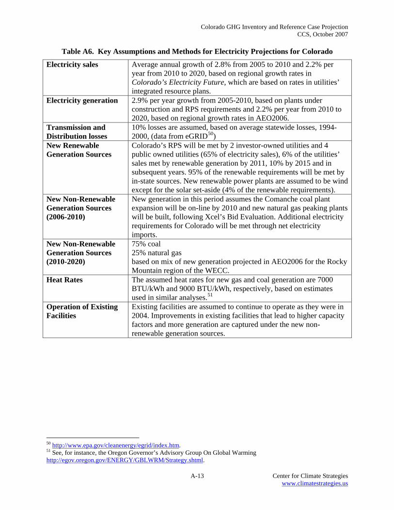
Colorado GHG Inventory and Reference Case Projection CCS, October 2007
A-13 Center for Climate Strategies www.climatestrategies.us
Table A6. Key Assumptions and Methods for Electricity Projections for Colorado
Electricity sales Average annual growth of 2.8% from 2005 to 2010 and 2.2% per year from 2010 to 2020, based on regional growth rates in Colorado’s Electricity Future, which are based on rates in utilities’ integrated resource plans.
Electricity generation 2.9% per year growth from 2005-2010, based on plants under construction and RPS requirements and 2.2% per year from 2010 to 2020, based on regional growth rates in AEO2006.
Transmission and Distribution losses
10% losses are assumed, based on average statewide losses, 1994-2000, (data from eGRID50)
New Renewable Generation Sources
Colorado’s RPS will be met by 2 investor-owned utilities and 4 public owned utilities (65% of electricity sales), 6% of the utilities’ sales met by renewable generation by 2011, 10% by 2015 and in subsequent years. 95% of the renewable requirements will be met by in-state sources. New renewable power plants are assumed to be wind except for the solar set-aside (4% of the renewable requirements).
New Non-Renewable Generation Sources (2006-2010)
New generation in this period assumes the Comanche coal plant expansion will be on-line by 2010 and new natural gas peaking plants will be built, following Xcel’s Bid Evaluation. Additional electricity requirements for Colorado will be met through net electricity imports.
New Non-Renewable Generation Sources (2010-2020)
75% coal 25% natural gas based on mix of new generation projected in AEO2006 for the Rocky Mountain region of the WECC.
Heat Rates The assumed heat rates for new gas and coal generation are 7000 BTU/kWh and 9000 BTU/kWh, respectively, based on estimates used in similar analyses.51
Operation of Existing Facilities
Existing facilities are assumed to continue to operate as they were in 2004. Improvements in existing facilities that lead to higher capacity factors and more generation are captured under the new non-renewable generation sources.
50 http://www.epa.gov/cleanenergy/egrid/index.htm. 51 See, for instance, the Oregon Governor’s Advisory Group On Global Warming http://egov.oregon.gov/ENERGY/GBLWRM/Strategy.shtml.
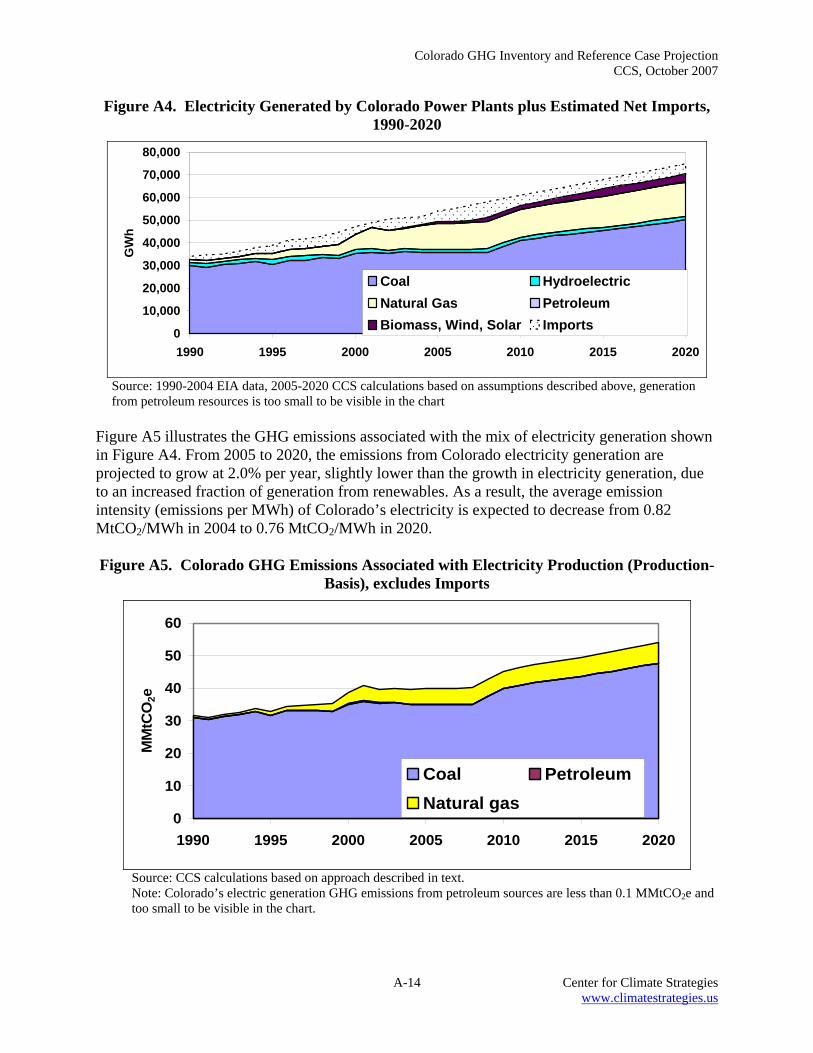
Colorado GHG Inventory and Reference Case Projection CCS, October 2007
A-14 Center for Climate Strategies www.climatestrategies.us
Figure A4. Electricity Generated by Colorado Power Plants plus Estimated Net Imports, 1990-2020
0
10,000
20,000
30,000
40,000
50,000
60,000
70,000
80,000
1990 1995 2000 2005 2010 2015 2020
GW
h
Coal HydroelectricNatural Gas PetroleumBiomass, Wind, Solar Imports
Source: 1990-2004 EIA data, 2005-2020 CCS calculations based on assumptions described above, generation from petroleum resources is too small to be visible in the chart
Figure A5 illustrates the GHG emissions associated with the mix of electricity generation shown in Figure A4. From 2005 to 2020, the emissions from Colorado electricity generation are projected to grow at 2.0% per year, slightly lower than the growth in electricity generation, due to an increased fraction of generation from renewables. As a result, the average emission intensity (emissions per MWh) of Colorado’s electricity is expected to decrease from 0.82 MtCO2/MWh in 2004 to 0.76 MtCO2/MWh in 2020.
Figure A5. Colorado GHG Emissions Associated with Electricity Production (Production-
Basis), excludes Imports
0
10
20
30
40
50
60
1990 1995 2000 2005 2010 2015 2020
MM
tCO
2e
Coal PetroleumNatural gas
Source: CCS calculations based on approach described in text. Note: Colorado’s electric generation GHG emissions from petroleum sources are less than 0.1 MMtCO2e and too small to be visible in the chart.
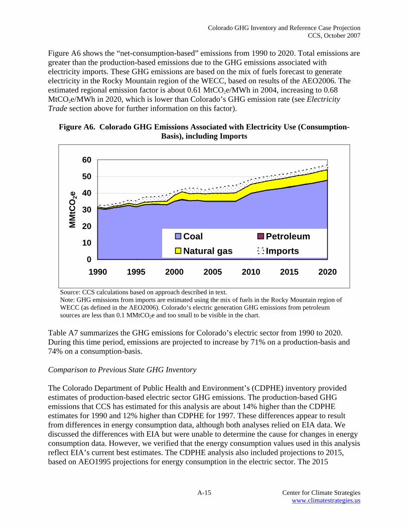
Colorado GHG Inventory and Reference Case Projection CCS, October 2007
A-15 Center for Climate Strategies www.climatestrategies.us
Figure A6 shows the “net-consumption-based” emissions from 1990 to 2020. Total emissions are greater than the production-based emissions due to the GHG emissions associated with electricity imports. These GHG emissions are based on the mix of fuels forecast to generate electricity in the Rocky Mountain region of the WECC, based on results of the AEO2006. The estimated regional emission factor is about 0.61 MtCO2e/MWh in 2004, increasing to 0.68 MtCO2e/MWh in 2020, which is lower than Colorado’s GHG emission rate (see Electricity Trade section above for further information on this factor).
Figure A6. Colorado GHG Emissions Associated with Electricity Use (Consumption-
Basis), including Imports
0
10
20
30
40
50
60
1990 1995 2000 2005 2010 2015 2020
MM
tCO
2e
Coal PetroleumNatural gas Imports
Source: CCS calculations based on approach described in text. Note: GHG emissions from imports are estimated using the mix of fuels in the Rocky Mountain region of WECC (as defined in the AEO2006). Colorado’s electric generation GHG emissions from petroleum sources are less than 0.1 MMtCO2e and too small to be visible in the chart.
Table A7 summarizes the GHG emissions for Colorado’s electric sector from 1990 to 2020. During this time period, emissions are projected to increase by 71% on a production-basis and 74% on a consumption-basis. Comparison to Previous State GHG Inventory The Colorado Department of Public Health and Environment’s (CDPHE) inventory provided estimates of production-based electric sector GHG emissions. The production-based GHG emissions that CCS has estimated for this analysis are about 14% higher than the CDPHE estimates for 1990 and 12% higher than CDPHE for 1997. These differences appear to result from differences in energy consumption data, although both analyses relied on EIA data. We discussed the differences with EIA but were unable to determine the cause for changes in energy consumption data. However, we verified that the energy consumption values used in this analysis reflect EIA’s current best estimates. The CDPHE analysis also included projections to 2015, based on AEO1995 projections for energy consumption in the electric sector. The 2015

Colorado GHG Inventory and Reference Case Projection CCS, October 2007
A-16 Center for Climate Strategies www.climatestrategies.us
emissions estimates from the CDPHE analysis were 50.2 MMtCO2e, only 1.6% larger than the estimates from this analysis, 49.5 MMtCO2e.
Table A7. Colorado GHG Emissions from Electric Sector, Production and Consumption-based estimates, 1990-2020 (MMtCO2e).
1990 1995 2000 2005 2010 2015 2020 Electricity Production Based 31.6 32.9 38.7 39.8 45.3 49.5 54.0 Coal 30.9 31.6 35.1 34.9 40.0 43.7 47.6 CO2 30.8 31.5 34.9 34.7 39.8 43.5 47.4 CH4 and N2O 0.15 0.15 0.17 0.17 0.20 0.21 0.23 Natural Gas 0.71 1.3 3.5 4.9 5.2 5.8 6.3 CO2 0.71 1.27 3.53 4.88 5.22 5.76 6.34 CH4 and N2O 0.00 0.00 0.00 0.00 0.00 0.01 0.01 Oil 0.02 0.02 0.08 0.02 0.02 0.02 0.02 CO2 0.02 0.02 0.08 0.02 0.02 0.02 0.02 CH4 and N2O 0.00 0.00 0.00 0.00 0.00 0.00 0.00 Wood (CH4 and N2O) 0.000 0.000 0.000 0.001 0.001 0.001 0.001 Net Imported Electricity 1.0 2.5 2.2 3.1 3.0 4.5 3.0 Electricity Consumption Based 32.7 35.4 40.9 42.9 48.2 54.0 57.0
Note: Assumes electricity production from renewable fuels are based on 2004 RPS requirements. Updates to the Reference Case Projection At the request of the Climate Action Panel (CAP), the reference case projections for the Electricity Supply sector were modified to include the effects of Colorado’s 2007 RPS law that increased requirements (relative to the state’s 2004 RPS) for IOUs to use renewable fuel resources. The reference case was also modified to incorporate the effects for House Bill (HB) 1146 to increase demand-side management (DSM) requirements for electricity. It was assumed that the fuel resource mix meeting the RPS is the same as that assumed in the 30% RPS policy developed by the CAP’s Policy Work Group (PWG). In 2020, wind energy is approximately 85% of RPS generation, and photovoltaic (PV), solar thermal, small hydro, biomass and geothermal are about 3% each. In addition, total electricity demand was reduced relative to the original reference case in response to certain DSM activities as discussed for the RCI sector. The effect of this is a reduction in the overall emissions associated with energy use, and also a reduction of the direct impact of the RPS program as this is based on a percentage of total electricity sales in the state. The RPS law requires Investor-Owned Utilities (IOUs) to provide 20% renewable energy by 2020 and non-IOUs (e.g., municipal utilities and rural electric cooperatives) to provide 10%. The law also includes incentive clauses for in-state generation, community-based projects and solar energy. The following assumptions were made for the purpose of revising the emissions projections under the 2007 RPS law:
• In-state generation constitutes 80% of the RPS generation for IOUs; and this energy receives 125% credit.
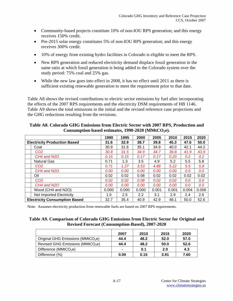
Colorado GHG Inventory and Reference Case Projection CCS, October 2007
A-17 Center for Climate Strategies www.climatestrategies.us
• Community-based projects constitute 10% of non-IOU RPS generation; and this energy receives 150% credit.
• Pre-2015 solar energy constitutes 5% of non-IOU RPS generation; and this energy receives 300% credit.
• 10% of energy from existing hydro facilities in Colorado is eligible to meet the RPS.
• New RPS generation and reduced electricity demand displace fossil generation in the same ratio at which fossil generation is being added to the Colorado system over the study period: 75% coal and 25% gas.
• While the new law goes into effect in 2008, it has no effect until 2011 as there is sufficient existing renewable generation to meet the requirement prior to that date.
Table A8 shows the revised contributions to electric sector emissions by fuel after incorporating the effects of the 2007 RPS requirements and the electricity DSM requirements of HB 1146. Table A9 shows the total emissions in the initial and the revised reference case projections and the GHG reductions resulting from the revisions. Table A8. Colorado GHG Emissions from Electric Sector with 2007 RPS, Production and
Consumption-based estimates, 1990-2020 (MMtCO2e). 1990 1995 2000 2005 2010 2015 2020 Electricity Production Based 31.6 32.9 38.7 39.8 45.3 47.6 50.0 Coal 30.9 31.6 35.1 34.9 40.0 42.1 44.2 CO2 30.8 31.5 34.9 34.7 39.8 41.9 43.9 CH4 and N2O 0.15 0.15 0.17 0.17 0.20 0.2 0.2 Natural Gas 0.71 1.3 3.5 4.9 5.2 5.5 5.8 CO2 0.71 1.27 3.53 4.88 5.22 5.5 5.8 CH4 and N2O 0.00 0.00 0.00 0.00 0.00 0.0 0.0 Oil 0.02 0.02 0.08 0.02 0.02 0.02 0.02 CO2 0.02 0.02 0.08 0.02 0.02 0.0 0.0 CH4 and N2O 0.00 0.00 0.00 0.00 0.00 0.0 0.0 Wood (CH4 and N2O) 0.000 0.000 0.000 0.001 0.001 0.004 0.006 Net Imported Electricity 1.0 2.5 2.2 3.1 2.9 2.4 2.6 Electricity Consumption Based 32.7 35.4 40.9 42.9 48.1 50.0 52.6
Note: Assumes electricity production from renewable fuels are based on 2007 RPS requirements.
Table A9. Comparison of Colorado GHG Emissions from Electric Sector for Original and Revised Forecast (Consumption-Based), 2007-2020
2007 2010 2015 2020 Original GHG Emissions (MMtCO2e) 44.4 48.2 52.0 57.0 Revised GHG Emissions (MMtCO2e) 44.4 48.2 50.0 52.6 Difference (MMtCO2e) - 0.1 2.0 4.3 Difference (%) 0.00 0.15 3.91 7.60

Colorado GHG Inventory and Reference Case Projection CCS, October 2007
B-1 Center for Climate Strategies www.climatestrategies.us
Appendix B. Residential, Commercial, and Industrial (RCI) Fuel Combustion Overview Activities in the RCI52 sectors produce carbon dioxide (CO2), methane (CH4), and nitrous oxide (N2O) emissions when fuels are combusted to provide space heating, process heating, and other applications. CO2 accounts for over 99% of these emissions on a million metric tons (MMt) of CO2 equivalent (CO2e) basis in Colorado. In addition, since these sectors consume electricity, one can also attribute emissions associated with electricity generation to these sectors in proportion to their electricity use.53 If emissions from the generation of the electricity they consume are not included, the RCI sectors are between them the third-largest source of gross greenhouse gas (GHG) emissions in Colorado. Direct use of oil, natural gas, coal, and wood in the RCI sectors accounted for an estimated 21.2 MMtCO2e (18%) of gross GHG emissions in 2005.54 Emissions and Reference Case Projections Emissions from direct fuel use were estimated using the United States Environmental Protection Agency’s (US EPA) State Greenhouse Gas Inventory Tool (SGIT) software and the methods provided in the Emission Inventory Improvement Program (EIIP) guidance document for RCI fossil fuel combustion.55 The default data used in SGIT for Colorado are from United States Department of Energy (US DOE) Energy Information Administration’s (EIA) State Energy Data (SED). The SGIT default data for Colorado were revised using the most recent data available, which includes: (1) 2002 SED information for all fuel types;56 (2) 2003 SED information for coal, and for wood and wood waste;57 (3) 2003 and 2004 SED information for natural gas;6 (4) 2003 and 2004 SED information for petroleum (distillate oil, kerosene and liquefied petroleum
52 The industrial sector includes emissions associated with agricultural energy use and fuel used by the fossil fuel production industry. 53 Emissions associated with the electricity supply sector (presented in Appendix A) have been allocated to each of the RCI sectors for comparison of those emissions to the fuel-consumption-based emissions presented in Appendix B. Note that this comparison is provided for information purposes and that emissions estimated for the electricity supply sector are not double-counted in the total emissions for the state. One could similarly allocate GHG emissions from natural gas transmission and distribution, other fuels production, and transport-related GHG sources to the RCI sectors based on their direct use of gas and other fuels, but we have not done so here due to the difficulty of ascribing these emissions to particular end-users. Emissions associated with the transportation sector are provided in Appendix C and emissions associated with fossil fuel production and distribution are provided in Appendix E. 54 Emissions estimates from wood combustion include only N2O and CH4. Carbon dioxide emissions from biomass combustion are assumed to be “net zero”, consistent with US EPA and Intergovernmental Panel on Climate Change (IPCC) methodologies, and any net loss of carbon stocks due to biomass fuel use should be accounted for in the land use and forestry analysis. 55 GHG emissions were calculated using SGIT, with reference to EIIP, Volume VIII: Chapter 1 “Methods for Estimating Carbon Dioxide Emissions from Combustion of Fossil Fuels”, August 2004, and Chapter 2 “Methods for Estimating Methane and Nitrous Oxide Emissions from Stationary Combustion”, August 2004. 56 EIA State Energy Data 2002, Data through 2002, released June 30, 2006, (http://www.eia.doe.gov/emeu/states/state.html?q_state_a=co&q_state=COLORADO). 57 EIA State Energy Data 2003 revisions for all fuels, and first release of 2004 information for natural gas and petroleum, (http://www.eia.doe.gov/emeu/states/_seds_updates.html).

Colorado GHG Inventory and Reference Case Projection CCS, October 2007
B-2 Center for Climate Strategies www.climatestrategies.us
gas) consumption;6 (5) 2004 electricity consumption data from the EIA’s State Electricity Profiles;58 and (6) 2005 natural gas consumption data from the EIA’s Natural Gas Navigator.59 Note that the EIIP methods for the industrial sector exclude from CO2 emission estimates the amount of carbon that is stored in products produced from fossil fuels for non-energy uses. For example, the methods account for carbon stored in petrochemical feedstocks, and in liquefied petroleum gases (LPG) and natural gas used as feedstocks by chemical manufacturing plants (i.e., not used as fuel), as well as carbon stored in asphalt and road oil produced from petroleum. The carbon storage assumptions for these products are explained in detail in the EIIP guidance document.60 The fossil fuel categories for which the EIIP methods are applied in the SGIT software to account for carbon storage include the following categories: asphalt and road oil, coking coal, distillate fuel, feedstocks (naphtha with a boiling range of less than 401 degrees Fahrenheit), feedstocks (other oils with boiling ranges greater than 401 degrees Fahrenheit), LPG, lubricants, miscellaneous petroleum products, natural gas, pentanes plus,61 petroleum coke, residual fuel, still gas, and waxes. Data on annual consumption of the fuels in these categories as chemical industry feedstocks were obtained from the EIA SED. Reference case emissions from direct fuel combustion were estimated based on fuel consumption forecasts from EIA’s Annual Energy Outlook 2006 (AEO2006),62 with adjustments for Colorado’s projected population63 and employment growth. Colorado employment data for the manufacturing (goods-producing) and non-manufacturing (commercial or services-providing) sectors were obtained from the Colorado Department of Labor and Employment.64 Regional employment data for the same sectors were obtained from EIA for the EIA’s Mountain region.65 Finally, as discussed at the end of this appendix, these growth projections were modified to reflect recent legislation and a settlement agreement leading to increased demand-side management (DSM) requirements in Colorado. Table B1 shows historic and projected growth rates for electricity sales by sector. Table B2 shows historic and projected growth rates for energy use by sector and fuel type before incorporating the effects of recent DSM requirements (see discussion under “Updates to the Reference Case Projections). For the residential sector, the rate of population growth is expected to be about 2.5% annually between 2004 and 2020; this demographic trend is reflected in the growth rates for residential fuel consumption. Based on the Colorado Department of Labor and Employment’s 10-year forecast (2004 to 2014), commercial and industrial employment are 58 EIA Electric Power Annual 2005 - State Data Tables, (http://www.eia.doe.gov/cneaf/electricity/epa/epa_sprdshts.html). 59 EIA Natural Gas Navigator (http://tonto.eia.doe.gov/dnav/ng/ng_cons_sum_dcu_SCO_a.htm). 60 EIIP, Volume VIII: Chapter 1 “Methods for Estimating Carbon Dioxide Emissions from Combustion of Fossil Fuels”, August 2004. 61 A mixture of hydrocarbons, mostly pentanes and heavier fractions, extracted from natural gas. 62 EIA AEO2006 with Projections to 2030, (http://www.eia.doe.gov/oiaf/aeo/index.html). 63 Population data for 1990 are from the Colorado State Demography Office (http://www.dola.state.co.us/demog/AllHist1.cfm). Population for 2000 and 2005 and forecasts for 2010 and 2025 are taken from the Colorado Data Book (http://www.state.co.us/oed/business-development/colorado-data-book.cfm). 64 Colorado Department of Labor and Employment, Colorado Industry and Occupational Projections, Released June 2006 (http://www.coworkforce.com/lmi/oeo/oeo.asp). 65 AEO2006 employment projections for EIA’s Mountain region obtained through special request from EIA (dated September 27, 2006).

Colorado GHG Inventory and Reference Case Projection CCS, October 2007
B-3 Center for Climate Strategies www.climatestrategies.us
projected to increase at compound annual rates of 2.8% and 2.7%, respectively, and these growth rates are reflected in the growth rates in energy use shown in Table B2 for the two sectors. The 2004-to-2014 commercial and industrial employment growth rates were carried forward to 2020 for the purpose of estimating emissions for the reference case projections. These estimates of growth relative to population and employment reflect expected responses of the economy — as simulated by the EIA’s National Energy Modeling System — to changing fuel and electricity prices and changing technologies, as well as to structural changes within each sector (such as shifts in subsectoral shares and in energy use patterns).
Table B1. Electricity Sales Annual Growth Rates, Historical and Projected
Sector 1990-2004* 2004-2020** Residential 3.4% 1.9% Commercial 2.6% 2.9% Industrial 4.2% 1.9% Total 3.0% 2.4%
* 1990-2004 compound annual growth rates calculated from Colorado electricity sales by year from EIA state electricity profiles (Table 8), http://www.eia.doe.gov/cneaf/electricity/st_profiles/e_profiles_sum.html. ** 2004-2020 compound annual growth rate for total for all three sectors taken from forecast for the energy supply sector (see Appendix A). Growth rates for individual sectors estimated based on the proportion of the individual sector’s growth rate to the total growth rate for 1990 to 2004.
Table B2. Historic and Projected Average Annual Growth in Energy Use in Colorado, by
Sector and Fuel, 1990-2020
1990-2004* 2005-2010** 2010-2015** 2015-2020** Residential natural gas 1.9% 2.9% 2.3% 2.1% petroleum 4.9% 1.5% 1.6% 1.2% wood -2.8% 1.4% -0.3% 0.1% coal 9.5% 1.3% -0.9% -0.8% Commercial natural gas -0.5% 2.3% 4.1% 3.4% petroleum 0.7% -0.5% 2.4% 1.9% wood -1.6% 1.0% 1.6% 1.2% coal 13.9% 0.9% 1.6% 1.2% Industrial natural gas 4.6% 2.8% 1.8% 1.8% petroleum 3.2% 3.8% 3.2% 2.6% wood -14.6% 4.4% 3.6% 3.5% coal -6.4% 2.4% 1.5% 1.3%
* Compound annual growth rates calculated from EIA SED historical consumption by sector and fuel type for Colorado. Latest year for which EIA SED information was available for each fuel type is 2003 for coal and wood/wood waste, 2004 for petroleum (distillate oil, kerosene, and liquefied petroleum gas), and 2005 for natural gas. Petroleum includes distillate fuel, kerosene, and liquefied petroleum gases for all sectors plus residual oil for the commercial and industrial sectors. ** Figures for growth periods starting after 2004 are calculated from AEO2006 projections for EIA’s Mountain region, adjusted for Colorado’s projected population for the residential sector, projections for non-manufacturing employment for the commercial sector, and projections for manufacturing employment for the industrial sector.
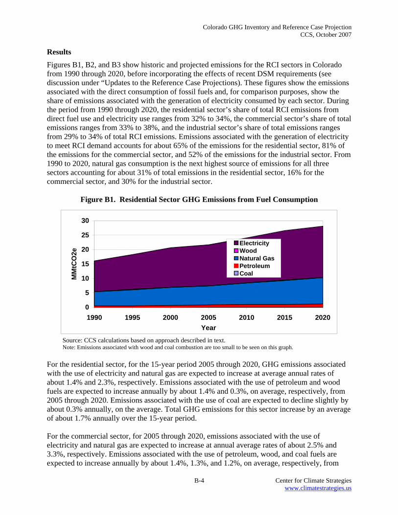
Colorado GHG Inventory and Reference Case Projection CCS, October 2007
B-4 Center for Climate Strategies www.climatestrategies.us
Results Figures B1, B2, and B3 show historic and projected emissions for the RCI sectors in Colorado from 1990 through 2020, before incorporating the effects of recent DSM requirements (see discussion under “Updates to the Reference Case Projections). These figures show the emissions associated with the direct consumption of fossil fuels and, for comparison purposes, show the share of emissions associated with the generation of electricity consumed by each sector. During the period from 1990 through 2020, the residential sector’s share of total RCI emissions from direct fuel use and electricity use ranges from 32% to 34%, the commercial sector’s share of total emissions ranges from 33% to 38%, and the industrial sector’s share of total emissions ranges from 29% to 34% of total RCI emissions. Emissions associated with the generation of electricity to meet RCI demand accounts for about 65% of the emissions for the residential sector, 81% of the emissions for the commercial sector, and 52% of the emissions for the industrial sector. From 1990 to 2020, natural gas consumption is the next highest source of emissions for all three sectors accounting for about 31% of total emissions in the residential sector, 16% for the commercial sector, and 30% for the industrial sector.
Figure B1. Residential Sector GHG Emissions from Fuel Consumption
0
5
10
15
20
25
30
1990 1995 2000 2005 2010 2015 2020Year
MM
tCO
2e
ElectricityWoodNatural GasPetroleumCoal
Source: CCS calculations based on approach described in text. Note: Emissions associated with wood and coal combustion are too small to be seen on this graph.
For the residential sector, for the 15-year period 2005 through 2020, GHG emissions associated with the use of electricity and natural gas are expected to increase at average annual rates of about 1.4% and 2.3%, respectively. Emissions associated with the use of petroleum and wood fuels are expected to increase annually by about 1.4% and 0.3%, on average, respectively, from 2005 through 2020. Emissions associated with the use of coal are expected to decline slightly by about 0.3% annually, on the average. Total GHG emissions for this sector increase by an average of about 1.7% annually over the 15-year period. For the commercial sector, for 2005 through 2020, emissions associated with the use of electricity and natural gas are expected to increase at annual average rates of about 2.5% and 3.3%, respectively. Emissions associated with the use of petroleum, wood, and coal fuels are expected to increase annually by about 1.4%, 1.3%, and 1.2%, on average, respectively, from
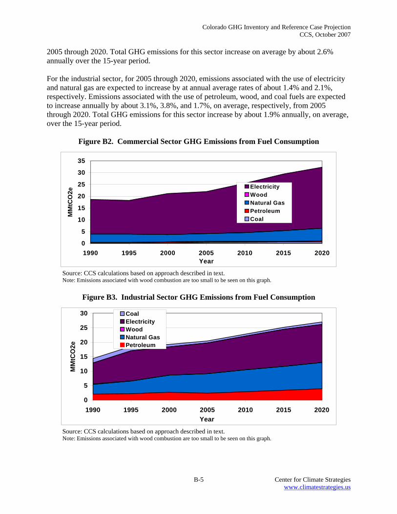
Colorado GHG Inventory and Reference Case Projection CCS, October 2007
B-5 Center for Climate Strategies www.climatestrategies.us
2005 through 2020. Total GHG emissions for this sector increase on average by about 2.6% annually over the 15-year period. For the industrial sector, for 2005 through 2020, emissions associated with the use of electricity and natural gas are expected to increase by at annual average rates of about 1.4% and 2.1%, respectively. Emissions associated with the use of petroleum, wood, and coal fuels are expected to increase annually by about 3.1%, 3.8%, and 1.7%, on average, respectively, from 2005 through 2020. Total GHG emissions for this sector increase by about 1.9% annually, on average, over the 15-year period.
Figure B2. Commercial Sector GHG Emissions from Fuel Consumption
0
5
10
15
20
25
30
35
1990 1995 2000 2005 2010 2015 2020Year
MM
tCO
2e
ElectricityWoodNatural GasPetroleumCoal
Source: CCS calculations based on approach described in text. Note: Emissions associated with wood combustion are too small to be seen on this graph.
Figure B3. Industrial Sector GHG Emissions from Fuel Consumption
0
5
10
15
20
25
30
1990 1995 2000 2005 2010 2015 2020Year
MM
tCO
2e
CoalElectricityWoodNatural GasPetroleum
Source: CCS calculations based on approach described in text. Note: Emissions associated with wood combustion are too small to be seen on this graph.
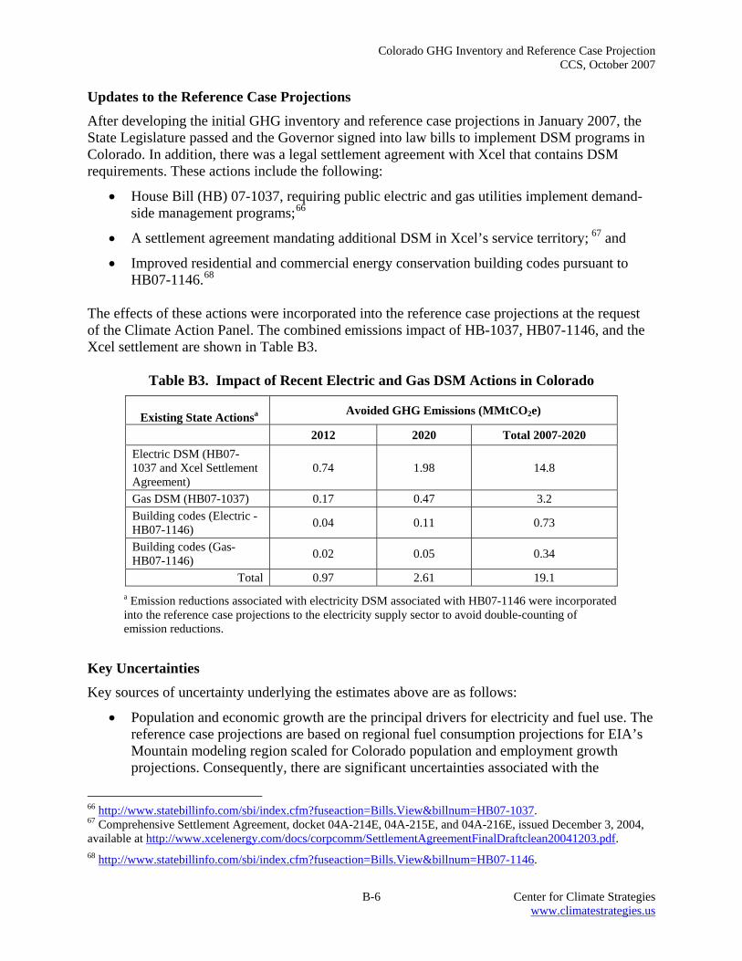
Colorado GHG Inventory and Reference Case Projection CCS, October 2007
B-6 Center for Climate Strategies www.climatestrategies.us
Updates to the Reference Case Projections After developing the initial GHG inventory and reference case projections in January 2007, the State Legislature passed and the Governor signed into law bills to implement DSM programs in Colorado. In addition, there was a legal settlement agreement with Xcel that contains DSM requirements. These actions include the following:
• House Bill (HB) 07-1037, requiring public electric and gas utilities implement demand-side management programs;66
• A settlement agreement mandating additional DSM in Xcel’s service territory; 67 and
• Improved residential and commercial energy conservation building codes pursuant to HB07-1146.68
The effects of these actions were incorporated into the reference case projections at the request of the Climate Action Panel. The combined emissions impact of HB-1037, HB07-1146, and the Xcel settlement are shown in Table B3.
Table B3. Impact of Recent Electric and Gas DSM Actions in Colorado
Existing State Actionsa Avoided GHG Emissions (MMtCO2e)
2012 2020 Total 2007-2020 Electric DSM (HB07-1037 and Xcel Settlement Agreement)
0.74 1.98 14.8
Gas DSM (HB07-1037) 0.17 0.47 3.2 Building codes (Electric - HB07-1146) 0.04 0.11 0.73
Building codes (Gas- HB07-1146) 0.02 0.05 0.34
Total 0.97 2.61 19.1 a Emission reductions associated with electricity DSM associated with HB07-1146 were incorporated into the reference case projections to the electricity supply sector to avoid double-counting of emission reductions.
Key Uncertainties Key sources of uncertainty underlying the estimates above are as follows:
• Population and economic growth are the principal drivers for electricity and fuel use. The reference case projections are based on regional fuel consumption projections for EIA’s Mountain modeling region scaled for Colorado population and employment growth projections. Consequently, there are significant uncertainties associated with the
66 http://www.statebillinfo.com/sbi/index.cfm?fuseaction=Bills.View&billnum=HB07-1037. 67 Comprehensive Settlement Agreement, docket 04A-214E, 04A-215E, and 04A-216E, issued December 3, 2004, available at http://www.xcelenergy.com/docs/corpcomm/SettlementAgreementFinalDraftclean20041203.pdf. 68 http://www.statebillinfo.com/sbi/index.cfm?fuseaction=Bills.View&billnum=HB07-1146.

Colorado GHG Inventory and Reference Case Projection CCS, October 2007
B-7 Center for Climate Strategies www.climatestrategies.us
projections. Future work should attempt to base projections of GHG emissions on fuel consumption estimates specific to Colorado to the extent that such data become available.
• The AEO2006 projections assume no large long-term changes in relative fuel and electricity prices, relative to current price levels and to US DOE projections for fuel prices. Price changes would influence consumption levels and, to the extent that price trends for competing fuels differ, may encourage switching among fuels, and thereby affect emissions estimates.
• The exception to the AEO2006 assumption of no large changes in prices or fuels consumption is the AEO2006 reference case projections for industrial coal consumption. The AEO2006 model’s forecast for the EIA’s Mountain region assumes that new coal-to-liquids plants would be constructed near active coal mines when low-sulfur distillate prices reach high enough levels to make coal-to-liquids processing economic. Plants are assumed to be co-production plants with generation capacity of 758 MW and the capability of producing 33,200 barrels of liquid fuel per day. The technology assumed is similar to an integrated gasification combined cycle plant, first converting the coal feedstock to gas, and then subsequently converting the synthetic gas to liquid hydrocarbons using the Fisher-Tropsch process. As a result, AEO2006 projections assume a rather significant increase in coal consumption by the coal-to-liquids industrial sector starting in 2011. For the EIA’s Mountain region, this sector accounts for 17.5% of total coal consumption in 2011 and 63% of total coal consumption in 2020, with an annual growth rate of 26% from 2011 to 2020.69 This increase in coal consumption, associated with the installation of coal-to-liquids plants starting in 2011, was excluded from the industrial coal consumption forecasts for Colorado because it is considered to represent technology that is beyond the “business-as-usual” assumptions associated with the reference case projections for the industrial coal consumption sector.
69 Coal Market Module of the National Energy Modeling System 2006, as described in Assumptions to the Annual Energy Outlook 2006, Coal Market Module, Report #: DOE/EIA-0554(2006), March 2006 (http://www.eia.doe.gov/oiaf/aeo/assumption/index.html).
Colorado GHG Inventory and Reference Case Projection CCS, October 2007
C-1 Center for Climate Strategies www.climatestrategies.us
Appendix C. Transportation Energy Use Overview Fuel use in the transportation sector is the second largest source of greenhouse gas (GHG) emissions in Colorado – accounting for 24% of Colorado’s gross GHG emissions in 2005. Carbon dioxide (CO2) accounts for about 96% of transportation GHG emissions from fuel use. Most of the remaining GHG emissions from the transportation sector are due to nitrous oxide (N2O) emissions from gasoline engines. Emissions and Reference Case Projections Greenhouse gas emissions for 1990 through 2002 were estimated using United States Environmental Protection Agency’s (US EPA) State Greenhouse Gas Inventory Tool (SGIT) and the methods provided in the Emission Inventory Improvement Program (EIIP) guidance document for the sector.70,71 For onroad vehicles, the CO2 emission factors are expressed in units of pounds per million British Thermal Units (lb/MMBTU), and the methane (CH4) and N2O emission factors are both in units of grams per vehicle miles traveled (g/VMT). Key assumptions in this analysis are listed in Table C1. The default data within SGIT were used to estimate emissions, with the most recently available fuel consumption data (2002) from United States Department of Energy (US DOE) Energy Information Administration (EIA) State Energy Data (SED) added.72 The default VMT data in SGIT were replaced with state-level annual VMT data from the Colorado Department of Transportation (CDOT).73 State-level VMT figures were allocated to vehicle types using the vehicle mix data provided by the Colorado Department of Public Health and Environment (CDPHE).74 Onroad gasoline and diesel emissions were forecast based on VMT projections provided by the Denver Regional Council of Governments (DRCOG), the North Front Range Transportation and Air Quality Planning Council (NFRTAQPC), the Pikes Peak Area Council of Governments (PPACG), and CDPHE.75,76,77 VMT projections from DRCOG were applied to VMT for Adams, Arapahoe, Boulder, Douglas, Denver, and Jefferson counties. Projections from NFRTAQPC were applied to Larimer and Weld counties, and projections from PPACG were applied to El Paso County. Vehicle miles traveled for all other counties were forecast using the 2002-2012 growth rate (assumed to extend to 2020) from the Colorado State Implementation Plan for
70 CO2 emissions were calculated using SGIT, with reference to EIIP, Volume VIII: Chapter. 1. “Methods for Estimating Carbon Dioxide Emissions from Combustion of Fossil Fuels”, August 2004. 71 CH4 and N2O emissions were calculated using SGIT, with reference to EIIP, Volume VIII: Chapter. 3. “Methods for Estimating Methane and Nitrous Oxide Emissions from Mobile Combustion”, August 2004. 72 EIA, State Energy Consumption, Price, and Expenditure Estimates (SED), http://www.eia.doe.gov/emeu/states/_seds.html 73Brad Beckham, Environmental Programs Branch Manager, Colorado Department of Transportation. 74 Barbara MacRae, Air Pollution Control Division Technical Services Program, Colorado Department of Public Health and Environment. 75 Erik Sabina, Regional Transportation Modeler, Denver Regional Council of Governments. 76 Andres Gomez, Regional Transportation Modeler, North Front Range MPO. 77 2005-2010 and 2007-2012 Transportation Improvement Programs, PPACG, http://www.ppacg.org/Trans/trans.htm.
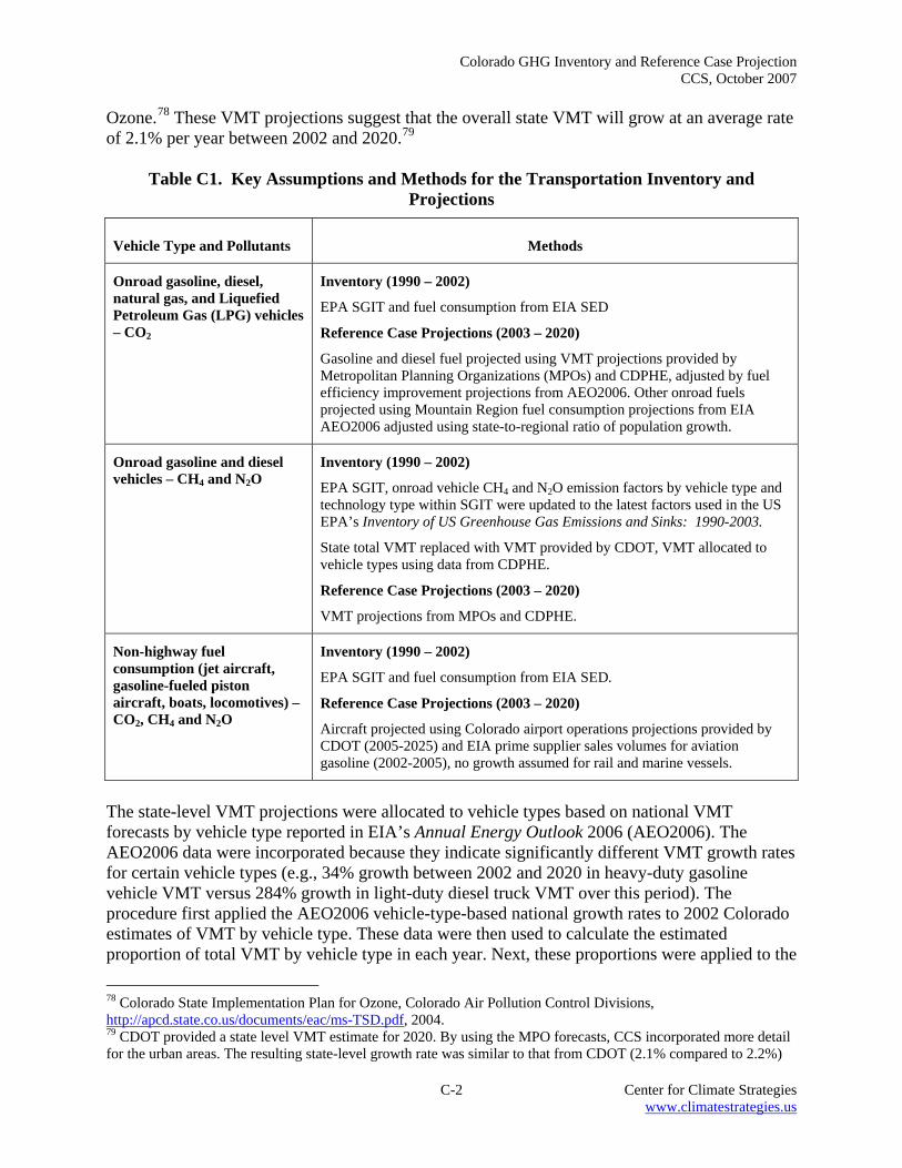
Colorado GHG Inventory and Reference Case Projection CCS, October 2007
C-2 Center for Climate Strategies www.climatestrategies.us
Ozone.78 These VMT projections suggest that the overall state VMT will grow at an average rate of 2.1% per year between 2002 and 2020.79
Table C1. Key Assumptions and Methods for the Transportation Inventory and
Projections
Vehicle Type and Pollutants Methods
Onroad gasoline, diesel, natural gas, and Liquefied Petroleum Gas (LPG) vehicles – CO2
Inventory (1990 – 2002)
EPA SGIT and fuel consumption from EIA SED
Reference Case Projections (2003 – 2020)
Gasoline and diesel fuel projected using VMT projections provided by Metropolitan Planning Organizations (MPOs) and CDPHE, adjusted by fuel efficiency improvement projections from AEO2006. Other onroad fuels projected using Mountain Region fuel consumption projections from EIA AEO2006 adjusted using state-to-regional ratio of population growth.
Onroad gasoline and diesel vehicles – CH4 and N2O
Inventory (1990 – 2002)
EPA SGIT, onroad vehicle CH4 and N2O emission factors by vehicle type and technology type within SGIT were updated to the latest factors used in the US EPA’s Inventory of US Greenhouse Gas Emissions and Sinks: 1990-2003.
State total VMT replaced with VMT provided by CDOT, VMT allocated to vehicle types using data from CDPHE.
Reference Case Projections (2003 – 2020)
VMT projections from MPOs and CDPHE.
Non-highway fuel consumption (jet aircraft, gasoline-fueled piston aircraft, boats, locomotives) – CO2, CH4 and N2O
Inventory (1990 – 2002)
EPA SGIT and fuel consumption from EIA SED.
Reference Case Projections (2003 – 2020)
Aircraft projected using Colorado airport operations projections provided by CDOT (2005-2025) and EIA prime supplier sales volumes for aviation gasoline (2002-2005), no growth assumed for rail and marine vessels.
The state-level VMT projections were allocated to vehicle types based on national VMT forecasts by vehicle type reported in EIA’s Annual Energy Outlook 2006 (AEO2006). The AEO2006 data were incorporated because they indicate significantly different VMT growth rates for certain vehicle types (e.g., 34% growth between 2002 and 2020 in heavy-duty gasoline vehicle VMT versus 284% growth in light-duty diesel truck VMT over this period). The procedure first applied the AEO2006 vehicle-type-based national growth rates to 2002 Colorado estimates of VMT by vehicle type. These data were then used to calculate the estimated proportion of total VMT by vehicle type in each year. Next, these proportions were applied to the
78 Colorado State Implementation Plan for Ozone, Colorado Air Pollution Control Divisions, http://apcd.state.co.us/documents/eac/ms-TSD.pdf, 2004. 79 CDOT provided a state level VMT estimate for 2020. By using the MPO forecasts, CCS incorporated more detail for the urban areas. The resulting state-level growth rate was similar to that from CDOT (2.1% compared to 2.2%)

Colorado GHG Inventory and Reference Case Projection CCS, October 2007
C-3 Center for Climate Strategies www.climatestrategies.us
estimates for total VMT in the state for each year to yield vehicle-specific VMT estimates and compound annual average growth rates displayed in Tables C2 and C3, respectively.
Table C2. Colorado Vehicle Miles Traveled Estimates (millions)
Vehicle Type 2002 2005 2010 2015 2020 Heavy-Duty Diesel Vehicle 1,188 1,374 1,644 1,924 2,213Heavy-Duty Gasoline Vehicle 499 555 617 703 792Light-Duty Diesel Truck 50 60 85 119 167Light-Duty Diesel Vehicle 21 25 36 50 70Light-Duty Gasoline Truck 12,333 13,180 14,701 16,266 17,679Light-Duty Gasoline Vehicle 11,918 12,736 14,206 15,719 17,084Motorcycle 91 98 109 120 131Total 26,098 28,027 31,397 34,903 38,135
Table C3. Colorado Vehicle Miles Traveled Compound Annual Growth Rates
Vehicle Type 2002-2005 2005-2010 2010-2015 2015-2020 Heavy-Duty Diesel Vehicle 4.97% 3.65% 3.20% 2.83% Heavy-Duty Gasoline Vehicle 3.66% 2.13% 2.65% 2.40% Light-Duty Diesel Truck 6.47% 7.21% 7.06% 6.93% Light-Duty Diesel Vehicle 6.47% 7.21% 7.06% 6.93% Light-Duty Gasoline Truck 2.24% 2.21% 2.04% 1.68% Light-Duty Gasoline Vehicle 2.24% 2.21% 2.04% 1.68% Motorcycle 2.24% 2.21% 2.04% 1.68%
Onroad gasoline and diesel fuel consumption was forecast by developing a set of growth factors that adjusted the VMT projections to account for improvements in fuel efficiency. Fuel efficiency projections were taken from EIA’s AEO2006. These projections suggest onroad fuel consumption growth rates of 1.2% per year for gasoline and 3.3% per year for diesel between 2002 and 2020. Gasoline consumption estimates for 1990-2002 were adjusted by subtracting ethanol consumption. While the historical ethanol consumption suggests continued growth, projections for ethanol consumption in Colorado were not available. Therefore, ethanol consumption was assumed to remain at the 2002 level (2.5% of total gasoline consumption) in the reference case projections. Biodiesel and other biofuel consumption were not included in this inventory, because historical and projection data were not available for these fuels. Emissions for aircraft operations for 1990 to 2002 were based on SGIT methods and fuel consumption from EIA SED. The consumption of international bunker fuels is included in jet fuel consumption from EIA. This fuel consumption associated with international air flights should not be included in the state inventory (as much of it is actually consumed out of state); however, data were not available to subtract this consumption from total jet fuel estimates. The 2002 estimates were then projected to 2005 in order to apply post-2005 projection data available from CDOT (as described below). Jet fuel emissions were projected based on 2002 and 2005 total operations for Denver International Airport, provided by CDOT. Aviation gasoline
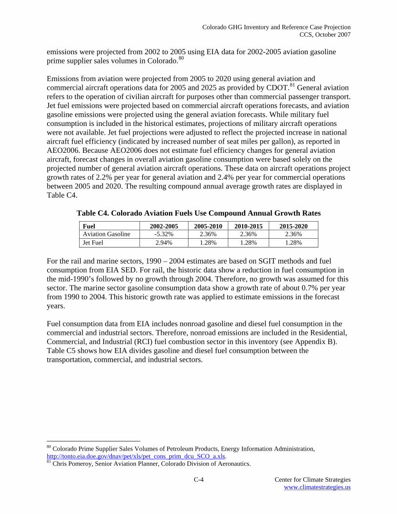
Colorado GHG Inventory and Reference Case Projection CCS, October 2007
C-4 Center for Climate Strategies www.climatestrategies.us
emissions were projected from 2002 to 2005 using EIA data for 2002-2005 aviation gasoline prime supplier sales volumes in Colorado.80 Emissions from aviation were projected from 2005 to 2020 using general aviation and commercial aircraft operations data for 2005 and 2025 as provided by CDOT.81 General aviation refers to the operation of civilian aircraft for purposes other than commercial passenger transport. Jet fuel emissions were projected based on commercial aircraft operations forecasts, and aviation gasoline emissions were projected using the general aviation forecasts. While military fuel consumption is included in the historical estimates, projections of military aircraft operations were not available. Jet fuel projections were adjusted to reflect the projected increase in national aircraft fuel efficiency (indicated by increased number of seat miles per gallon), as reported in AEO2006. Because AEO2006 does not estimate fuel efficiency changes for general aviation aircraft, forecast changes in overall aviation gasoline consumption were based solely on the projected number of general aviation aircraft operations. These data on aircraft operations project growth rates of 2.2% per year for general aviation and 2.4% per year for commercial operations between 2005 and 2020. The resulting compound annual average growth rates are displayed in Table C4.
Table C4. Colorado Aviation Fuels Use Compound Annual Growth Rates
Fuel 2002-2005 2005-2010 2010-2015 2015-2020 Aviation Gasoline -5.32% 2.36% 2.36% 2.36% Jet Fuel 2.94% 1.28% 1.28% 1.28%
For the rail and marine sectors, 1990 – 2004 estimates are based on SGIT methods and fuel consumption from EIA SED. For rail, the historic data show a reduction in fuel consumption in the mid-1990’s followed by no growth through 2004. Therefore, no growth was assumed for this sector. The marine sector gasoline consumption data show a growth rate of about 0.7% per year from 1990 to 2004. This historic growth rate was applied to estimate emissions in the forecast years. Fuel consumption data from EIA includes nonroad gasoline and diesel fuel consumption in the commercial and industrial sectors. Therefore, nonroad emissions are included in the Residential, Commercial, and Industrial (RCI) fuel combustion sector in this inventory (see Appendix B). Table C5 shows how EIA divides gasoline and diesel fuel consumption between the transportation, commercial, and industrial sectors. 80 Colorado Prime Supplier Sales Volumes of Petroleum Products, Energy Information Administration, http://tonto.eia.doe.gov/dnav/pet/xls/pet_cons_prim_dcu_SCO_a.xls. 81 Chris Pomeroy, Senior Aviation Planner, Colorado Division of Aeronautics.
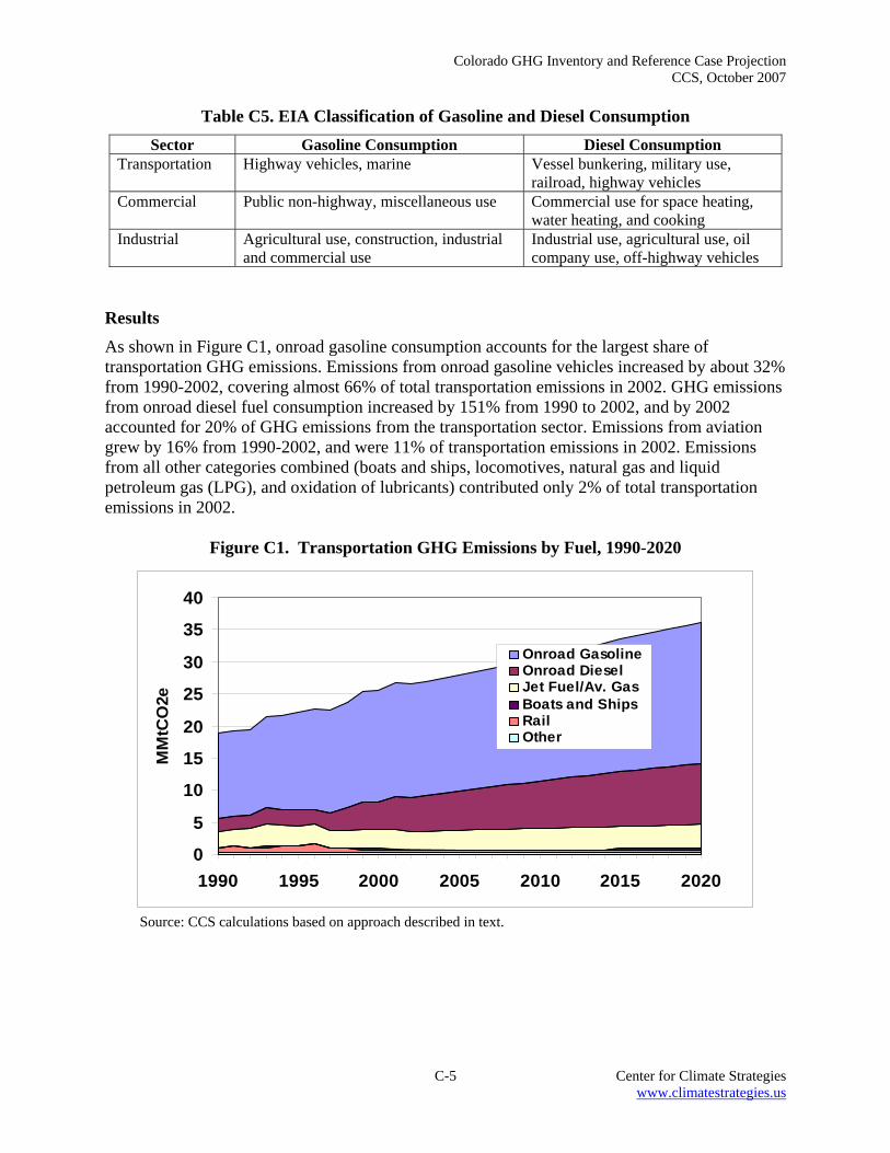
Colorado GHG Inventory and Reference Case Projection CCS, October 2007
C-5 Center for Climate Strategies www.climatestrategies.us
Table C5. EIA Classification of Gasoline and Diesel Consumption Sector Gasoline Consumption Diesel Consumption
Transportation Highway vehicles, marine Vessel bunkering, military use, railroad, highway vehicles
Commercial Public non-highway, miscellaneous use Commercial use for space heating, water heating, and cooking
Industrial Agricultural use, construction, industrial and commercial use
Industrial use, agricultural use, oil company use, off-highway vehicles
Results As shown in Figure C1, onroad gasoline consumption accounts for the largest share of transportation GHG emissions. Emissions from onroad gasoline vehicles increased by about 32% from 1990-2002, covering almost 66% of total transportation emissions in 2002. GHG emissions from onroad diesel fuel consumption increased by 151% from 1990 to 2002, and by 2002 accounted for 20% of GHG emissions from the transportation sector. Emissions from aviation grew by 16% from 1990-2002, and were 11% of transportation emissions in 2002. Emissions from all other categories combined (boats and ships, locomotives, natural gas and liquid petroleum gas (LPG), and oxidation of lubricants) contributed only 2% of total transportation emissions in 2002.
Figure C1. Transportation GHG Emissions by Fuel, 1990-2020
0
5
10
15
20
25
30
35
40
1990 1995 2000 2005 2010 2015 2020
MM
tCO
2e
Onroad GasolineOnroad DieselJet Fuel/Av. GasBoats and ShipsRailOther
Source: CCS calculations based on approach described in text.
Colorado GHG Inventory and Reference Case Projection CCS, October 2007
C-6 Center for Climate Strategies www.climatestrategies.us
Key Uncertainties Projections of VMT and Biofuels Consumption One source of uncertainty in the projections of transportation sector GHG emissions presented above is the future-year vehicle mix, which was calculated based on national growth rates for specific vehicle types. These growth rates may not reflect vehicle-specific VMT growth rates for the state. Also, onroad gasoline and diesel growth rates may be slightly overestimated because increased consumption of biofuels between 2002 and 2020 was not taken into account (due to a lack of data). International Bunker Fuels The consumption of international bunker fuels included in jet fuel consumption from EIA is another uncertainty. At least the bulk of this fuel consumption associated with international air flights should not be included in the state inventory (as much of it is actually consumed out of Colorado airspace); data were not, however, available to allow this consumption to be subtracted from total jet fuel use estimates. Another uncertainty associated with aviation emissions is the use of general aviation forecasts to project aviation gasoline consumption. General aviation aircraft consume both jet fuel and aviation gasoline, but fuel- specific data were not available. Also, jet fuel consumption includes consumption by military aircraft; projections of military aircraft operations were not available.
Colorado GHG Inventory and Reference Case Projection CCS, October 2007
D-1 Center for Climate Strategies www.climatestrategies.us
Appendix D. Industrial Processes Overview Emissions in the industrial processes category span a wide range of activities, and reflect non-combustion sources of greenhouse gas (GHG) emissions from several industrial processes. This sector accounted for about 3% of Colorado’s gross GHG emissions in 2005. The industrial processes that exist in Colorado, and for which emissions are estimated in this inventory, include the following:
• Carbon Dioxide (CO2) from: - Production of cement, lime, and soda ash - Consumption of limestone, dolomite, and soda ash;
• Hydrofluorocarbons (HFCs), perfluorocarbons (PFCs), and sulfur hexafluoride (SF6) from semiconductor manufacture;
• SF6 from transformers used in electric power transmission and distribution (T&D) systems; and
• HFCs and PFCs from consumption of substitutes for ozone-depleting substances (ODS) used in cooling and refrigeration equipment.
Other industrial processes that are sources of GHG emissions but are not found in Colorado include the following:
• Nitrous oxide (N2O) from nitric and adipic acid production;
• PFCs from aluminum production;
• HFCs from HCFC-22 production; and
• SF6 from magnesium production and processing. Emissions and Reference Case Projections GHG emissions for 1990 through 2005 were estimated using the State Greenhouse Gas Inventory Tool (SGIT) and the methods provided in the Emissions Inventory Improvement Project (EIIP) guidance document for this sector.82 Table D1 identifies for each emissions source category the information needed for input into SGIT to calculate emissions, the data sources used, and the historical years for which emissions were calculated based on the availability of data. Table D2 lists the data sources used to quantify activities related to industrial process emissions, the annual compound growth rates implied by the estimates of future activity used, and the years for which the reference case projections were calculated.
82 GHG emissions were calculated using SGIT, with reference to the Emission Inventory Improvement Program, Volume VIII: Chapter. 6. “Methods for Estimating Non-Energy Greenhouse Gas Emissions from Industrial Processes”, August 2004. This document is referred to as “EIIP” below.
Colorado GHG Inventory and Reference Case Projection CCS, October 2007
D-2 Center for Climate Strategies www.climatestrategies.us
Results Figures D1 and D2 show historic and projected emissions for the Colorado industrial processes sector from 1990 to 2020. Total gross GHG emissions were about 2.1 million metric tons (MMt) of carbon dioxide equivalent (CO2e) in 2000 (2% of total emissions), rising to about 5.9 MMtCO2e in 2020 (4% of total emissions). Emissions from the overall industrial processes category are expected to grow rapidly, as shown in Figures D1 and D2, with emissions growth almost entirely due to the increasing use of HFCs and PFCs in refrigeration and air conditioning equipment.
Table D1. Approach to Estimating Historical Emissions
Source Category Time
Period Required Data for
SGIT Data Source Cement Manufacturing - Clinker Production
1990 - 2002
Metric tons (Mt) of clinker produced each year.
US Geological Survey (USGS) in Cement: Annual Report. Note: USGS aggregates production for groups of states for confidentiality purposes. In the SGIT, aggregated production is divided by the number of states for which production is aggregated to estimate production for a given state. The number of states included in an aggregate total may vary from one year to the next. For example, the USGS generally aggregates clinker production from Colorado and Wyoming. SGIT divides this aggregated production by two to estimate Colorado’s clinker production. This is a limitation in SGIT and may result in overestimating or underestimating production for a given state.
Cement Manufacturing - Masonry Cement Production
1990 and
1996-2000
Mt of masonry cement produced each year.
USGS in Cement: Annual Report. Note: Data limitations are the same as described for cement production. Data are not available for some years; in those cases, data for the closest year to that for which data were missing was used as a surrogate to fill in production data for missing years (e.g., 1996 production used for 1995, and 2000 production used for 2001 and 2002.
Lime Manufacture 1990, 1995, 2000, and
2005
Mt of high-calcium and dolomitic lime produced each year.
Colorado Department of Public Health and Environment (CDPHE), Air Pollution Control Division, Stationary Sources Program provided production data for two plants for several but not all years. Data for the closest year were used as surrogates to fill in production data for missing years (e.g., production data for 1996 were used for 1995). Production by type of lime (i.e., hydrated lime versus quicklime) produced was estimated using regional lime production data from USGS, Minerals Yearbook - Lime for various years (http://minerals.usgs.gov/ minerals/pubs/commodity/lime/index.html#mis). EIIP methods applied to remove water from hydrated lime production estimates. Then, national lime production data from USGS, Minerals Yearbook – Lime, was used to estimate amount of high-calcium and dolomitic lime.
Soda Ash Manufacture
Not available. One plant in Colorado produces soda ash. According to Chapter 6 of the EIIP guidance document, information is not available to determine how to estimate CO2e for the process used at this plant. Consequently, CO2e are not estimated for soda ash production.

Colorado GHG Inventory and Reference Case Projection CCS, October 2007
D-3 Center for Climate Strategies www.climatestrategies.us
Table D1. Approach to Estimating Historical Emissions (Continued) Source
Category Time
Period Required Data for
SGIT Data Source Limestone and Dolomite Consumption
1994 - 2002
Consumption of limestone and dolomite by industrial sectors.
For default data, the state's total limestone consumption (as reported by USGS) is multiplied by the ratio of national limestone consumption for industrial uses to total national limestone consumption. Additional information on these calculations, including a definition of industrial uses, is available in Chapter 6 of the EIIP guidance document.
Soda Ash 1990 - 2005
Consumption of soda ash used in consumer products such as glass, soap and detergents, paper, textiles, and food. Emissions based on state’s population and estimates of emissions per capita from the US EPA national GHG inventory.
USGS Minerals Yearbook, 2004: Volume I, Metals and Minerals, (http://minerals.usgs.gov/minerals/pubs/commodity/soda_ash/). For population data, see references for ODS substitutes.
ODS Substitutes 1990 - 2002
Based on state’s population and estimates of emissions per capita from the US EPA national GHG inventory.
-- Population data for 1990 from Colorado State Demography Office (http://www.dola.state.co.us/demog/AllHist1.cfm). Population for 2000 and 2005 and forecasts for 2010 and 2025 from the Colorado Data Book (http://www.state.co.us/oed/business-development/colorado-data-book.cfm). -- US 1990-2000 population from US Census Bureau (http://www.census.gov/popest/archives/EST90INTERCENSAL/US-EST90INT-01.html). -- US 2000-2005 population from US Census Bureau (http://www.census.gov/population/ projections/SummaryTabA1.xls).
Semiconductor Manufacturing
1990 - 2002
State and national value of semiconductor shipments for NAICS code 334413 (Semiconductor and Related Device Manufacturing). Method uses ratio of state-to-national value of semiconductor shipments to estimate state’s proportion of national emissions for 1990 - 2002.
National emissions from US EPA 2005 Inventory of US Greenhouse Gas Emissions and Sinks: 1990-2003 (http://www.epa.gov/climatechange/ emissions/usgginv_archive.html). Value of shipments from U.S Census Bureau's 1997 Economic Census (http://www.census.gov/econ/ census02/). For 1997, value of shipments for state was 1.8% of national total. In the 2002 Economic Census, value of shipments for sate was 1.9% of national total. Given the uncertainty of this method and that the proportion of state-to-national value of shipments in 2002 is very close to the proportion for 1997, the 1997 proportion was used for all years, rather than using the 1997 proportion for some years and 2002 proportion for others.
Electric Power T&D Systems
1990 - 2002
Emissions from 1990 to 2003 based on the national emissions per kilowatt-hour (kWh) and state's electricity use.
National emissions per kWh from US EPA 2005 Inventory of US Greenhouse Gas Emissions and Sinks: 1990-2003 (http://www.epa.gov/climatechange/ emissions/usgginv_archive.html).

Colorado GHG Inventory and Reference Case Projection CCS, October 2007
D-4 Center for Climate Strategies www.climatestrategies.us
Table D2. Approach to Estimating Projections Annual Growth Rates (%)
Source Category
Time Period
Projection Assumptions Data Source
2000 to
2005
2005to
2010
2010to
2015
2015to
2020 Cement Manufacturing - Clinker Production and Masonry Cement Production
2003 - 2020
Compound annual growth rate from Colorado Nonmetallic Minerals sector employment projections (2004-2014). Assumed growth is same for 2015 – 2020 as in previous periods.
Colorado Department of Labor and Employment; (http://www.coworkforce.com/lmi/oeo/oeo.asp).
1.2 1.2 1.2 1.2
Lime Manufacture
2006 - 2020
Ditto Ditto 1.2 1.2 1.2 1.2
Limestone and Dolomite Consumption
2003 - 2020
Ditto Ditto 1.2 1.2 1.2 1.2
Soda Ash Consumption
2003 - 2020
Growth between 2004 and 2009 is projected to be about 0.5% per year for US production. Assumed growth is same for 2010 – 2020.
Minerals Yearbook, 2005: Volume I, Soda Ash, (http://minerals.usgs.gov/minerals/pubs/commodity/soda_ash/soda_myb05.pdf).
0.5 0.5 0.5 0.5
ODS Substitutes 2003 - 2020
Based on national growth rate for use of ODS substitutes.
EPA, 2004 ODS substitutes cost study report (http://www.epa.gov/ozone/snap/emissions/TMP6si9htnvca.htm).
15.8 7.9 5.8 5.3
Semiconductor Manufacturing
2003 - 2020
National growth rate (based on aggregate for all stewardship program categories provided in referenced data source)
US Department of State, US Climate Action Report, May 2002, Washington, D.C., May 2002 (Table 5-7). (http://yosemite.epa.gov/oar/globalwarming.nsf/UniqueKeyLookup/SHSU5BNQ76/$File/ch5.pdf).
3.3 -6.2 -9.0 -2.8
Electric Power T&/D Systems
2003 - 2020
Ditto ditto 3.3 -6.2 -9.0 -2.8
Substitutes for Ozone-Depleting Substances (ODS) HFCs and PFCs are used as substitutes for ODS, most notably CFCs (CFCs are also potent warming gases) in compliance with the Montreal Protocol and the Clean Air Act Amendments of 1990.83 Even low amounts of HFC and PFC emissions, for example, from leaks and other
83 As noted in EIIP Chapter 6, ODS substitutes are primarily associated with refrigeration and air conditioning but also have many other uses such as fire extinguishers, solvent cleaning, aerosols, foam blowing, and sterilization. ODS substitutes depend on technology characteristics in a range of equipment. For the US national inventory, a detailed stock vintaging model was used, but this modeling approach has not been completed at the state level.
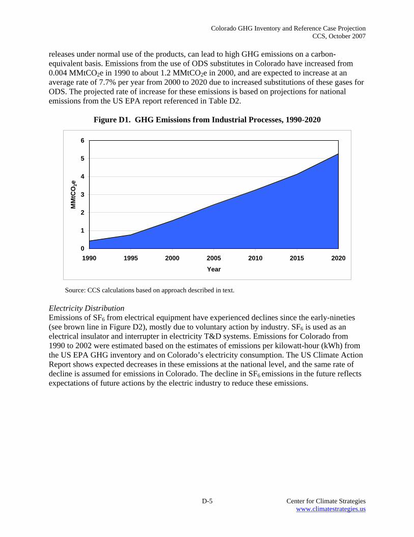
Colorado GHG Inventory and Reference Case Projection CCS, October 2007
D-5 Center for Climate Strategies www.climatestrategies.us
releases under normal use of the products, can lead to high GHG emissions on a carbon-equivalent basis. Emissions from the use of ODS substitutes in Colorado have increased from 0.004 MMtCO2e in 1990 to about 1.2 MMtCO2e in 2000, and are expected to increase at an average rate of 7.7% per year from 2000 to 2020 due to increased substitutions of these gases for ODS. The projected rate of increase for these emissions is based on projections for national emissions from the US EPA report referenced in Table D2.
Figure D1. GHG Emissions from Industrial Processes, 1990-2020
0
1
2
3
4
5
6
1990 1995 2000 2005 2010 2015 2020
Year
MM
tCO
2e
Source: CCS calculations based on approach described in text.
Electricity Distribution Emissions of SF6 from electrical equipment have experienced declines since the early-nineties (see brown line in Figure D2), mostly due to voluntary action by industry. SF6 is used as an electrical insulator and interrupter in electricity T&D systems. Emissions for Colorado from 1990 to 2002 were estimated based on the estimates of emissions per kilowatt-hour (kWh) from the US EPA GHG inventory and on Colorado’s electricity consumption. The US Climate Action Report shows expected decreases in these emissions at the national level, and the same rate of decline is assumed for emissions in Colorado. The decline in SF6 emissions in the future reflects expectations of future actions by the electric industry to reduce these emissions.

Colorado GHG Inventory and Reference Case Projection CCS, October 2007
D-6 Center for Climate Strategies www.climatestrategies.us
Figure D2. GHG Emissions from Industrial Processes, 1990-2020, by Source
0
1
2
3
4
5
1990 1995 2000 2005 2010 2015 2020
Year
MM
tCO
2e
Cement Manufacture Lime ManufactureLimestone & Dolomite Use (CO2) Soda Ash Use (CO2)ODS Substitutes (HFCs, SF6) Semiconductor Manf. (HFCs, SF6)Electricity Dist. (SF6)
Source: CCS calculations based on approach described in text.
Semiconductor Manufacture Emissions of SF6 and HFCs from the manufacture of semiconductors have experienced declines since 2000 (see yellow line in Figure D2). Emissions for Colorado from 1990 to 2002 were estimated based on the default estimates provided in SGIT, which uses the ratio of the state-to-national value of semiconductor shipments to estimate the state’s proportion of national emissions from the US EPA GHG inventory (US EPA 2005 Inventory of US Greenhouse Gas Emissions and Sinks: 1990-2003). The US Climate Action Report shows expected decreases in these emissions at the national level, and the same rate of decline is assumed for emissions in Colorado. The decline in emissions in the future reflects expectations of future actions by the semiconductor industry to reduce these emissions. Cement Manufacture Colorado has two cement plants that produce clinker (an intermediate product from which finished Portland and masonry cement are made). Clinker production releases CO2 when calcium carbonate (CaCO3) is heated in a cement kiln to form lime (calcium oxide) and CO2 (see Chapter 6 of the EIIP guidance document). Emissions are calculated by multiplying annual clinker production and annual production of masonry cement by emission factors for these processes. However, information on clinker and masonry cement production was not readily available; therefore, the default data provided in SGIT were used to calculate emissions (see black line in Figure D2). The growth rate for Colorado’s nonmetallic minerals sector (an annual average of 1.2%) was used to project emissions to 2020.
Colorado GHG Inventory and Reference Case Projection CCS, October 2007
D-7 Center for Climate Strategies www.climatestrategies.us
Lime Manufacture Lime is a manufactured product that is used in many chemical, industrial, and environmental applications including steel making, construction, pulp and paper manufacturing, and water and sewage treatment. Lime is manufactured by heating limestone (mostly CaCO3) in a kiln, creating calcium oxide and CO2. The CO2 is driven off as a gas and is normally emitted to the atmosphere, leaving behind a product known as quicklime. Some of this quicklime undergoes slaking (combining with water), which produces hydrated lime. The consumption of lime for certain uses, specifically the production of precipitated CaCO3 and refined sugar, results in the reabsorption of some airborne CO2 (see Chapter 6 of the EIIP guidance document). Emissions are estimated by multiplying the amount of high-calcium and dolomitic lime produced by emission factors for each product. The Colorado Department of Public Health and Environment (CDPHE) provided annual lime production data for two sugar refining plants for several but not all years. Lime production for years for which data were not available was estimated using the production data for the closest year as a surrogate (e.g., production data for 1996 used for 1995). Total production for the two plants was combined and then regional factors from the USGS were applied to total production to estimate the amount of hydrated lime and quicklime produced. EIIP methods were applied to remove the mass of water contained in the product from the hydrated lime production estimates. Then, national lime production data from the USGS was used to estimate the amount of high-calcium and dolomitic lime produced each year. These production figures were entered into the SGIT to calculate CO2 emissions (see dark blue line in Figure D2). The growth rate for Colorado’s nonmetallic minerals sector (i.e., 1.2% annual) was used to project emissions to 2020. Limestone and Dolomite Consumption Limestone and dolomite are basic raw materials used by a wide variety of industries, including the construction, agriculture, chemical, glass manufacturing, environmental pollution control, and metallurgical industries such as magnesium production.84 Recent historical data for Colorado were not available from the USGS; consequently, the default data provided in SGIT were used to calculate emissions for Colorado (see orange line in Figure D2). The growth rate for Colorado’s nonmetallic minerals sector (i.e., 1.2% annual) was used to project emissions to 2020. Soda Ash Consumption Commercial soda ash (sodium carbonate) is used in many consumer products such as glass, soap and detergents, paper, textiles, and food. CO2 is also released when soda ash is consumed (see Chapter 6 of the EIIP guidance document). SGIT estimates historical emissions (see dark pink line in Figure D2) based on the state’s population and national per capita emissions from the US EPA national GHG inventory. According to the USGS, this industry is expected to grow at an annual rate of 0.5% from 2004 through 2009 for the US as a whole. Information on growth
84 In accordance with EIIP Chapter 6 methods, emissions associated with the following uses of limestone and dolomite are not included in this category: (1) crushed limestone consumed for road construction or similar uses (because these uses do not result in CO2 emissions), (2) limestone used for agricultural purposes (which is counted under the methods for the agricultural sector), and (3) limestone used in cement production (which is counted in the methods for cement production).
Colorado GHG Inventory and Reference Case Projection CCS, October 2007
D-8 Center for Climate Strategies www.climatestrategies.us
trends for the soda ash industry for years later than 2009 was not available; the same (2004 – 2009) growth rate was therefore applied for estimating emissions through 2020. Key Uncertainties Key sources of uncertainty underlying the estimates above are as follows:
• Historical clinker production for the cement industry is uncertain because of the reliance on the SGIT method that divides aggregated clinker production (obtained from the USGS) for select states evenly between the states. In SGIT, production for Colorado and Wyoming is aggregated and divided evenly between the two states. Future work on this category should focus on obtaining actual clinker production data for 1990 through 2005 from plants located in Colorado.
• Since emissions from industrial processes are determined by the level of production in and the production processes of a few key industries, and, in some cases, of a few key plants, there is relatively high uncertainty regarding future emissions from the industrial processes category as a whole. Future emissions depend on the competitiveness of Colorado manufacturers in these industries, and the specific nature of the production processes used in plants in Colorado.
• The projected largest source of future industrial emissions, HFCs and PFCs used in cooling applications, is subject to several uncertainties as well. First, historical emissions are based on national estimates; Colorado-specific estimates are currently unavailable. For example, emissions will be driven by future choices regarding mobile and stationary air conditioning technologies and the use of refrigerants in commercial applications, for which several options currently exist.
• Greenhouse gases are emitted from several additional industrial processes that are not covered in the EIIP guidance documents, due in part to a lack of sufficient state data on non-energy uses of fossil fuels for these industrial processes. These sources include:
• Iron and Steel Production (CO2 and CH4);
• Ammonia Manufacture and Urea Application (CO2, CH4, N2O);
• Aluminum Production (CO2);
• Titanium Dioxide Production (CO2);
• Phosphoric Acid Production (CO2);
• CO2 Consumption (CO2);
• Ferroalloy Production (CO2);
• Petrochemical Production (CH4); and
• Silicon Carbide Production (CH4).
The CO2 emissions from the above CO2 sources (other than CO2 consumption and phosphoric acid production) result from the non-energy use of fossil fuels. Although the US EPA estimates emissions for these industries on a national basis, US EPA has not

Colorado GHG Inventory and Reference Case Projection CCS, October 2007
D-9 Center for Climate Strategies www.climatestrategies.us
developed methods for estimating the emissions at the state level due to data limitations. If state-level data on non-energy uses of fuels become available, future work should include an assessment of emissions for these other categories. The CDPHE’s report, Greeenhouse Gas Emission Inventory and Forecast, 1990 through 2015 (revised October 2002, Table 2.1.2), identifies the industrial sources that exist in Colorado but for which state-specific methods are not available to estimate GHG emissions.
Colorado GHG Inventory and Reference Case Projection CCS, October 2007
E-1 Center for Climate Strategies www.climatestrategies.us
Appendix E. Fossil Fuel Industries This appendix reports the greenhouse gas (GHG) emissions that are released during the production, processing, transmission, and distribution of fossil fuels. Known as fugitive emissions, these are methane (CH4) and carbon dioxide (CO2) gases released via leakage and venting at coal mines, oil and gas fields, fossil fuel processing facilities, and gas and oil pipelines. Nationally, fugitive emissions from natural gas systems, petroleum systems, and coal mines accounted for 2.8% of total US GHG emissions in 2004.85 In Colorado, this sector has somewhat higher emissions than the national average accounting for 9% of Colorado’s gross GHG emissions in 2005. Emissions associated with energy consumed by these processes are included in the residential, commercial and industrial sector emissions (see Appendix B). Oil and Gas Production Colorado currently ranks 12th in crude oil production among US states, totaling 63,000 barrels (bbls) per day and accounting for about 1% of US production.86 Proved state crude oil reserves sit at 225 million bbls, which is similarly about 1% of US totals. Oil production in Colorado peaked in 1988 at 88,000 bbls per day.87 Colorado has two petroleum refineries, with a combined crude oil distillation capacity of 94,000 bbls per day.88 Colorado currently produces almost two and a half times the amount of natural gas that it consumes. For example, in 2004, Colorado consumed 440 billion cubic feet (Bcf) and produced 1,079 Bcf. Since the year 2000, total natural gas production (combined conventional and unconventional sources) has increased by 44%.89 Unconventional oil and gas resources play an increasingly important role in the state. Colorado is a significant player in the coal bed methane (CBM) industry, placing first in the nation for CBM proved reserves and a close second to New Mexico for CBM production.90 United States Department of Energy (US DOE) Energy Information Administration (EIA) reports annual CBM production growth rates in Colorado averaging over 50% throughout the first half of the 1990s. Average CBM growth rates in the state had slowed to 3% annually between 2000 and 2005. Between 1999 and 2001, natural gas production from CBM accounted for about 60% of total natural gas production in state. The share of natural gas production from CBM has subsequently decreased as the growth in conventional gas has outpaced the growth in CBM production. CBM accounted for 47% of total Colorado natural gas production in 2005.
85 “The U.S. Inventory of Greenhouse Gas Emissions and Sinks”, United States Environmental Protection Agency (US EPA), 2005. 86 “Petroleum Profile: Colorado”, US DOE EIA website, October 2006, Accessed at <http://tonto.eia.doe.gov/oog/info/state/co.html> 87 “Petroleum Navigator”, US DOE EIA website, October 2006, Accessed at <http://tonto.eia.doe.gov/dnav/pet/hist/mcrfpco1a.htm> 88 IBID 89 “Natural Gas Navigator”, US DOE EIA website, September 2006, Accessed at <http://tonto.eia.doe.gov/dnav/ng/hist/n9050co2a.htm> 90 “Natural Gas Navigator”, US DOE EIA website, September 2006, Accessed at <http://tonto.eia.doe.gov/dnav/ng/ng_enr_cbm_a_EPG0_r52_Bcf_a.htm>

Colorado GHG Inventory and Reference Case Projection CCS, October 2007
E-2 Center for Climate Strategies www.climatestrategies.us
In addition, Colorado has the largest, and most commercially viable, oil shale deposits of any US state. While commercial oil shale production is a number of years away, high oil prices have brought renewed interest. There are currently 5 research and development proposals for in-situ technology pending approval by the United States Bureau of Land Management (BLM).91 A 2005 study projected a 12- to 16-year lag before the pilot tests initiated over the next few years lead to a production growth phase.92 Given the large uncertainty surrounding future production from oil shale in Colorado, especially in the 2006-2020 timeframe, this analysis does not include a specific estimate for oil shale production or for total GHG emissions from this process. While a high-level review of oil shale research projects was conducted, meaningful GHG emission intensity estimates could not be provided within the time constraints of this project. Oil and Gas Industry Emissions Emissions of CH4 and entrained CO2 can occur at many stages of production, processing, transmission, and distribution of oil and gas. With over 23,000 gas and oil wells in the state, 43 operational gas processing plants, 2 oil refineries, and over 32,000 miles of gas pipelines93, there are significant uncertainties associated with estimates of Colorado’s GHG emissions from this sector. This is compounded by the fact that there are no regulatory requirements to track CO2 or methane emissions. Therefore, estimates based on emissions measurements in Colorado are not possible at this time. The State Greenhouse Gas Inventory Tool (SGIT) developed by the United States Environmental Protection Agency (US EPA) facilitates the development of rough estimates of state-level GHG emissions.94 Methane emission estimates are calculated by multiplying emissions-related activity levels (e.g., miles of pipeline, number of compressor stations) by aggregate industry-average emission factors. Key information sources for the activity data are the US DOE EIA95 and American Gas Association’s annual publication Gas Facts.96 CH4 emissions were estimated using SGIT, with reference to the Emissions Inventory Improvement Project (EIIP) guidance document. Future projections of CH4 emissions from oil and gas systems are calculated based on the following key drivers:
• Consumption – See Appendix A, Electricity, and Appendix B, Residential, Commercial and Industrial Sector for assumptions used in projecting natural gas consumption in Colorado. Based on those assumptions, Colorado’s natural gas consumption is projected to decline slightly until 2010, and then grow at a rate of just over 2.5% annually.
• Production – Continued growth over the next few years in both conventional oil and gas, and CBM appears likely. Drilling permits reported by the Oil and Gas Conservation Commission
91 Kent Walters, BLM, White River Field Office manager 92 Bartis, James T. et al, Oil Shale development in the United States: prospects and policy issues. 2005. Rand Corporation. Prepared for the National Energy Technology Laboratory of the US Department of Energy. 93 Data from EIA and Gas Facts. 94 CH4 emissions were calculated using SGIT, with reference to Emission Inventory Improvement Program, Volume VIII: Chapter. 5. “Methods for Estimating Methane Emissions from Natural Gas and Oil Systems”, March 2005. 95 “Petroleum Navigator” and “Natural Gas Navigator”, US DOE EIA website, November 2006, Accessed at http://www.eia.doe.gov 96 American Gas Association “Gas Facts, A Statistical Record of the Gas Industry” Referenced annual publications from 1992 to 2004.
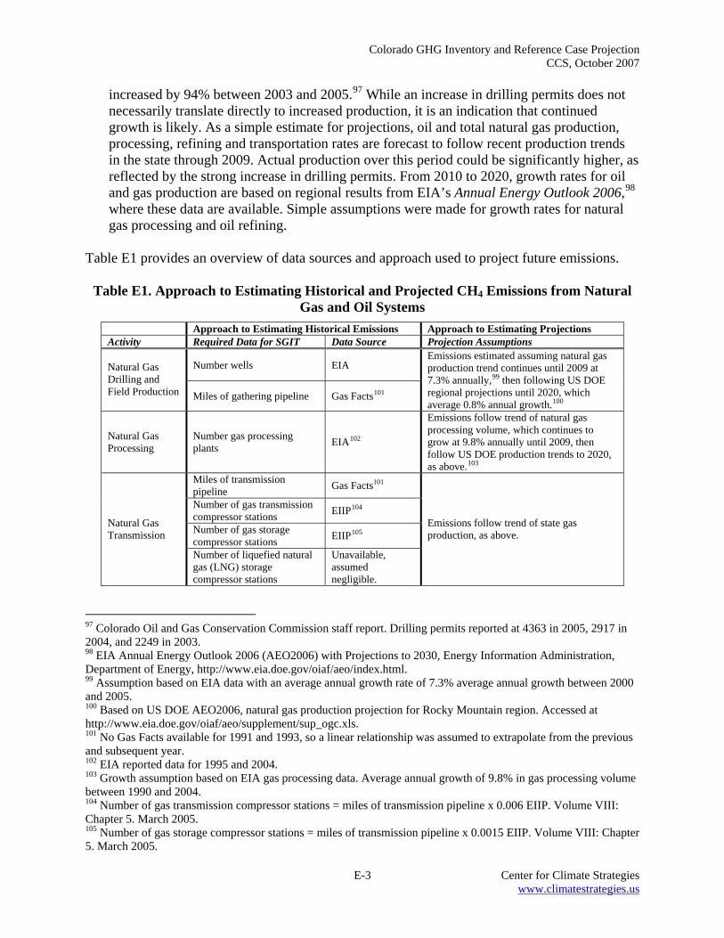
Colorado GHG Inventory and Reference Case Projection CCS, October 2007
E-3 Center for Climate Strategies www.climatestrategies.us
increased by 94% between 2003 and 2005.97 While an increase in drilling permits does not necessarily translate directly to increased production, it is an indication that continued growth is likely. As a simple estimate for projections, oil and total natural gas production, processing, refining and transportation rates are forecast to follow recent production trends in the state through 2009. Actual production over this period could be significantly higher, as reflected by the strong increase in drilling permits. From 2010 to 2020, growth rates for oil and gas production are based on regional results from EIA’s Annual Energy Outlook 2006,98 where these data are available. Simple assumptions were made for growth rates for natural gas processing and oil refining.
Table E1 provides an overview of data sources and approach used to project future emissions.
Table E1. Approach to Estimating Historical and Projected CH4 Emissions from Natural Gas and Oil Systems
Approach to Estimating Historical Emissions Approach to Estimating Projections Activity Required Data for SGIT Data Source Projection Assumptions
Number wells EIA Natural Gas Drilling and Field Production Miles of gathering pipeline Gas Facts101
Emissions estimated assuming natural gas production trend continues until 2009 at 7.3% annually,99 then following US DOE regional projections until 2020, which average 0.8% annual growth.100
Natural Gas Processing
Number gas processing plants EIA102
Emissions follow trend of natural gas processing volume, which continues to grow at 9.8% annually until 2009, then follow US DOE production trends to 2020, as above.103
Miles of transmission pipeline Gas Facts101
Number of gas transmission compressor stations EIIP104
Number of gas storage compressor stations EIIP105
Natural Gas Transmission
Number of liquefied natural gas (LNG) storage compressor stations
Unavailable, assumed negligible.
Emissions follow trend of state gas production, as above.
97 Colorado Oil and Gas Conservation Commission staff report. Drilling permits reported at 4363 in 2005, 2917 in 2004, and 2249 in 2003. 98 EIA Annual Energy Outlook 2006 (AEO2006) with Projections to 2030, Energy Information Administration, Department of Energy, http://www.eia.doe.gov/oiaf/aeo/index.html. 99 Assumption based on EIA data with an average annual growth rate of 7.3% average annual growth between 2000 and 2005. 100 Based on US DOE AEO2006, natural gas production projection for Rocky Mountain region. Accessed at http://www.eia.doe.gov/oiaf/aeo/supplement/sup_ogc.xls. 101 No Gas Facts available for 1991 and 1993, so a linear relationship was assumed to extrapolate from the previous and subsequent year. 102 EIA reported data for 1995 and 2004. 103 Growth assumption based on EIA gas processing data. Average annual growth of 9.8% in gas processing volume between 1990 and 2004. 104 Number of gas transmission compressor stations = miles of transmission pipeline x 0.006 EIIP. Volume VIII: Chapter 5. March 2005. 105 Number of gas storage compressor stations = miles of transmission pipeline x 0.0015 EIIP. Volume VIII: Chapter 5. March 2005.

Colorado GHG Inventory and Reference Case Projection CCS, October 2007
E-4 Center for Climate Strategies www.climatestrategies.us
Table E1. Approach to Estimating Historical and Projected CH4 Emissions from Natural Gas and Oil Systems (Continued)
Miles of distribution pipeline Gas Facts101 Total number of services Gas Facts Number of unprotected steel services
Ratio estimated from 2002 data107
Natural Gas Distribution
Number of protected steel services
Ratio estimated from 2002 data107
Distribution emissions follow state gas consumption trend.106
Oil Production Annual production EIA108
Emissions follow trend of state oil production, which is projected to grow at 1.9% annually until 2009109, then follow US DOE regional projections until 2020, which average 1.4% annual growth.110
Oil Refining Annual amount refined EIA111 Emissions projected to follow trend of 0.5% annual growth in state oil refining.112
Oil Transport Annual oil transported
Unavailable, assumed oil refined = oil transported
Emissions follow trend of state oil refining, as above.
Note that potential improvements to production, processing, and pipeline technologies resulting in GHG emissions reductions have not been accounted for in this analysis. A potentially significant source of CO2 that is not currently included in this inventory is that of ”entrained” CO2 in raw gas emerging from the ground. In some areas entrained CO2 can be significantly above pipeline specifications, and must be separated out at gas processing facilities. Depending on the level of entrained CO2 in Colorado coal bed methane produced, emissions of entrained CO2 from this source may be significant. Unfortunately, this data could not be obtained within the time constraints of this project. As noted above, this analysis also does not include a specific estimate for oil shale production. Note that any commercial development of oil shale in the region would result in increased carbon dioxide equivalent (CO2e) emissions from oil production, refining and transportation, and that no emissions from oil shale facilities are included in current forecasts. As production of oil from oil shale is expected to be energy- (and therefore GHG emissions-) intensive, any future oil shale development could have significant GHG implications.
106 Based on US DOE regional projections. 107 Gas Facts reported unprotected and protected steel services for 2002, but only total services for other years. Therefore the ratio of unprotected and protected steel services in 2002 was assumed to be the ratio for all other years (0.4891 for protected services and 0.0045 for unprotected services). This yields more congruent results than the EIIP guidance of using multipliers of 0.2841 for protected steel services, and 0.0879 for unprotected steel services. 108 Data extracted from the Petroleum Supply Annual for each year. 109 Based on EIA data, with an annual average oil production growth rate of 1.9% between 2000 and 2005. 110 Based on US DOE AEO2006, oil production projection for Rocky Mountain region. Accessed at http://www.eia.doe.gov/oiaf/aeo/supplement/sup_ogc.xls. 111 Refining assumed to be equal to the total input of crude oil into Petroleum Administration for Defense Districts (PADD) IV times the ratio of Colorado’s refining capacity to PADD IV’s total refining capacity. No data for 1995 and 1997, so linear relationship assumed from previous and subsequent years. 112 Based on EIA data, average growth in crude refined annually was 1.7% between 2000 and 2004.

Colorado GHG Inventory and Reference Case Projection CCS, October 2007
E-5 Center for Climate Strategies www.climatestrategies.us
Coal Production Emissions CH4 occurs naturally in coal seams, and is typically vented during mining operations for safety reasons. Coal mine methane emissions are usually considerably higher, per unit of coal produced, from underground mining than from surface mining.
Colorado has 13 operational coal mines, which together produced 38.5 million short tons of coal in 2005.113 Of Colorado’s 13 coal mines, 8 are underground and 5 are surface mines. In this inventory, CH4 emissions from coal mines are as reported by the US EPA, and include emissions from underground coal mines, surface mines, and post-mining activities.114 Coal mine CH4 projections are based on coal production projections provided by a contact at the Colorado Geological Survey.115 As a simple assumption for projections, CH4 emissions per unit coal mined for the three (underground, surface, and post-mining) categories of mining emission sources were assumed to hold constant at the 2004 level.116 Results Table E2 displays the estimated CH4 emissions from the fossil fuel industry in Colorado from 1990 to 2005, with projections to 2020. Emissions from this sector grew by 35% from 1990 to 2005, and are projected to increase by a further 22% from 2005 to 2020. The natural gas industry accounts for the majority of both GHG emissions and emissions growth in the fossil fuel industry as a whole.
Table E2. Methane Emissions and Projections from the Fossil Fuel Industry (Million Metric Tons CO2e) 1990 1995 2000 2005 2010 2015 2020Fossil Fuel Industry 7.5 7.0 9.3 10.1 11.8 12.1 12.3
Natural Gas Industry 3.1 3.3 4.8 5.0 6.5 6.8 7.3 Total Methane Emissions (CH4) 3.1 3.3 4.8 5.0 6.5 6.8 7.3 Total Entrained (CO2) n/a n/a n/a n/a n/a n/a n/a Production (methane emissions) 0.5 0.6 1.8 1.3 1.8 1.8 1.9 Processing 1.0 1.0 1.1 1.2 1.8 1.9 2.0 Methane Emissions (CH4) 1.0 1.0 1.1 1.2 1.8 1.9 2.0 Entrained Gas (CO2) n/a n/a n/a n/a n/a n/a n/a Transmission (methane emissions) 1.0 1.0 1.1 1.4 1.9 1.9 2.0 Distribution (methane emissions) 0.6 0.7 0.9 1.1 1.1 1.2 1.4
Oil Industry 0.2 0.2 0.2 0.2 0.2 0.2 0.2 Production (methane emissions) 0.2 0.2 0.1 0.2 0.2 0.2 0.2 Refineries (methane emissions) 0.0 0.0 0.0 0.0 0.0 0.0 0.0
Coal Mining (methane emissions) 4.2 3.5 4.3 4.9 5.1 5.1 4.8 Source: CCS calculations based on approach described in text.
113 EIA 114 Emissions from EPA Inventory of Greenhouse Gas Emissions and Sinks: 1990-2004 (April 2006) http://yosemite.epa.gov/oar/globalwarming.nsf/content/ResourceCenterPublicationsGHGEmissions USEmissionsInventory2006.html 115 Personal communication with Chris Carroll of the Colorado Geological Survey, December 2006. Coal production estimates given in million short tons annually at the following rates: 2006: 35, 2007: 39, 2008-2015: 40, 2016-2020: decline at 1% per year. 116 Based on 2004 EIA data, CH4 emission intensity calculated to average 0.127 metric tons CO2e per short ton produced coal.
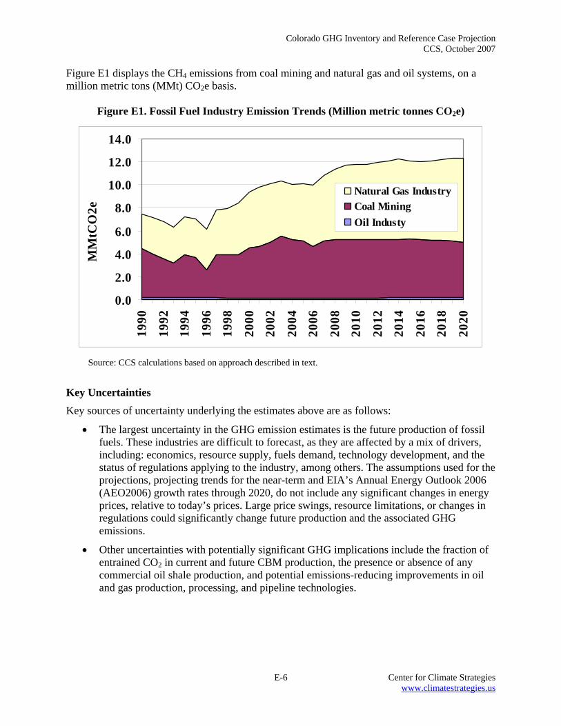
Colorado GHG Inventory and Reference Case Projection CCS, October 2007
E-6 Center for Climate Strategies www.climatestrategies.us
Figure E1 displays the CH4 emissions from coal mining and natural gas and oil systems, on a million metric tons (MMt) CO2e basis.
Figure E1. Fossil Fuel Industry Emission Trends (Million metric tonnes CO2e)
0.0
2.0
4.0
6.0
8.0
10.0
12.0
14.019
90
1992
1994
1996
1998
2000
2002
2004
2006
2008
2010
2012
2014
2016
2018
2020
MM
tCO
2e
Natural Gas IndustryCoal MiningOil Industy
Source: CCS calculations based on approach described in text.
Key Uncertainties Key sources of uncertainty underlying the estimates above are as follows:
• The largest uncertainty in the GHG emission estimates is the future production of fossil fuels. These industries are difficult to forecast, as they are affected by a mix of drivers, including: economics, resource supply, fuels demand, technology development, and the status of regulations applying to the industry, among others. The assumptions used for the projections, projecting trends for the near-term and EIA’s Annual Energy Outlook 2006 (AEO2006) growth rates through 2020, do not include any significant changes in energy prices, relative to today’s prices. Large price swings, resource limitations, or changes in regulations could significantly change future production and the associated GHG emissions.
• Other uncertainties with potentially significant GHG implications include the fraction of entrained CO2 in current and future CBM production, the presence or absence of any commercial oil shale production, and potential emissions-reducing improvements in oil and gas production, processing, and pipeline technologies.
Colorado GHG Inventory and Reference Case Projection CCS, October 2007
F-1 Center for Climate Strategies www.climatestrategies.us
Appendix F. Agriculture Overview The emissions discussed in this appendix refer to non-energy methane (CH4) and nitrous oxide (N2O) emissions from enteric fermentation, manure management, and agricultural soils. Emissions and sinks of carbon in agricultural soils are also covered. This sector accounted for about 8% of Colorado’s gross GHG emissions in 2005. Energy emissions related to agricultural practices (combustion of fossil fuels to power agricultural equipment) are included in the residential, commercial, and industrial (RCI) fuel consumption sector estimates. There are two livestock sources of greenhouse gas (GHG) emissions: enteric fermentation and manure management. Methane emissions from enteric fermentation are the result of normal digestive processes in ruminant and non-ruminant livestock. Microbes in the animal digestive system break down food and emit CH4 as a by-product. More CH4 is produced in ruminant livestock than in other animals because of digestive activity in the large fore-stomach to break down grasses and other high-fiber feeds. Methane and N2O emissions from the storage and treatment of livestock manure (e.g., in compost piles or anaerobic treatment lagoons) occur as a result of manure decomposition. The environmental conditions of decomposition drive the relative magnitude of emissions. In general, the more anaerobic the conditions are, the more CH4 is produced because decomposition is aided by CH4 producing bacteria that thrive in oxygen-limited (or oxygen-free) anaerobic conditions. Under aerobic conditions, N2O emissions are the dominant GHG emissions of concern. Emissions estimates from manure management are based on estimates of the volumes of manure that are stored and treated in livestock operations. Emissions from manure that is applied to agricultural soils as an amendment or deposited directly to pasture and grazing land by grazing animals are accounted for in inventories of emissions from agricultural soils. The management of agricultural soils can result in N2O emissions and in fluxes of carbon dioxide (CO2) that make soils net emitters or net sinks of carbon. In general, soil amendments that add nitrogen to soils can also result in N2O emissions. Nitrogen additions drive underlying soil nitrification and de-nitrification cycles, which produce N2O as a by-product. The emissions estimation methodologies used in this inventory account for several sources of N2O emissions from agricultural soils, including decomposition of crop residues, synthetic and organic fertilizer application, manure and sewage sludge application to soils, nitrogen fixation, and cultivation of histosols (high organic soils, such as wetlands or peatlands). Both direct and indirect emissions of N2O occur from the application of manure, fertilizer, and sewage sludge to agricultural soils. Direct emissions occur at the site of application, and indirect emissions occur when nitrogen leaches to groundwater or in surface runoff and is transported off-site before entering the nitrification/denitrification cycle. Methane and N2O emissions also result when crop residues are burned. Methane emissions occur during rice cultivation; however rice is not grown in Colorado. The net flux of CO2 in or out of agricultural soils depends on the balance of carbon losses from management practices and gains from organic matter inputs to the soil. Carbon dioxide is absorbed by plants through photosynthesis and ultimately becomes the carbon source for organic matter inputs to agricultural soils. When inputs are greater than losses, the soil accumulates carbon and there is a net sink of CO2 into agricultural soils. Conversely, soil disturbance from the
Colorado GHG Inventory and Reference Case Projection CCS, October 2007
F-2 Center for Climate Strategies www.climatestrategies.us
cultivation of histosols releases large stores of carbon from the soil to the atmosphere. Finally, the practice of adding limestone and dolomite to agricultural soils results in CO2 emissions. Emissions and Reference Case Projections
Methane and Nitrous Oxide GHG emissions for 1990 through 2005 were estimated using the United States Environmental Protection Agency’s (US EPA) State Greenhouse Gas Inventory Tool (SGIT) and the methods provided in the Emission Inventory Improvement Program (EIIP) guidance document for the sector.117 In general, the SGIT methodology applies emission factors developed for the US to activity data for the agriculture sector. Activity data include livestock population statistics, amounts of fertilizer applied to crops, and trends in manure management practices. This methodology is based on international guidelines developed by sector experts for preparing GHG emissions inventories.118 Data on crop production in Colorado from 1990 to 2005 and on the number of animals in the state from 1990 to 2002 were obtained from the USDA National Agriculture Statistical Service (NASS) and incorporated as defaults in SGIT.119 Data on fertilizer usage came from Commercial Fertilizers, a report from the Fertilizer Institute. The default data in SGIT accounting for the percentage of each livestock category using each type of manure management system was revised based on local data.120 Emissions from enteric fermentation and manure management were estimated based on the annual growth rate in emissions (million metric ton (MMt) carbon dioxide equivalent (CO2e) basis) associated with historical livestock populations in Colorado for 1990 to 2002. The dairy cattle population was assumed to continue growing at the historical (1990-2002) growth rate of 1.8% per year. All other livestock populations are assumed to remain at 2002 levels.121 Colorado has one hog farm of approximately 5,000 hogs that employs a manure digester. However, the emission reduction (0.001 MMtCO2e) from this operation does not have a significant effect on the statewide manure management emissions. Crop production data from the United States Department of Agriculture (USDA) National Agricultural Statistics Service (NASS) were available through 2005; therefore, N2O emissions from crop residues and crops that use nitrogen (nitrogen fixation) were calculated through 2005. Emissions for the other agricultural crop production practices categories (synthetic and organic fertilizers, agricultural residue burning) were calculated through 2002. Data were not available to
117 GHG emissions were calculated using SGIT, with reference to EIIP, Volume VIII: Chapter 8. “Methods for Estimating Greenhouse Gas Emissions from Livestock Manure Management”, August 2004; Chapter 10. “Methods for Estimating Greenhouse Gas Emissions from Agricultural Soil Management”, August 2004; and Chapter 11. “Methods for Estimating Greenhouse Gas Emissions from Field Burning of Agricultural Residues”, August 2004. 118 Revised 1996 1ntergovermental Panel on Climate Change Guidelines for National Greenhouse Gas Inventories, published by the National Greenhouse Gas Inventory Program of the IPCC, available at http://www.ipcc-nggip.iges.or.jp/public/gl/invs1.htm; and Good Practice Guidance and Uncertainty Management in National Greenhouse Gas Inventories, published in 2000 by the National Greenhouse Gas Inventory Program of the IPCC, available at: http://www.ipcc-nggip.iges.or.jp/public/gp/english/. 119 USDA, NASS (http://www.nass.usda.gov/Statistics_by_State/Colorado/index.asp). 120 Jessica Davis, Department of Soil and Crop Sciences, Colorado State University provided revised values for waste management system percentages. 121 Renee Picanso, Colorado Agricultural Statistics Service, recommended projecting dairy cattle populations based on historical data and assuming no growth for beef cattle.
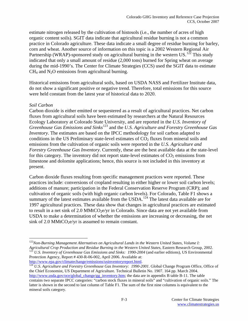
Colorado GHG Inventory and Reference Case Projection CCS, October 2007
F-3 Center for Climate Strategies www.climatestrategies.us
estimate nitrogen released by the cultivation of histosols (i.e., the number of acres of high organic content soils). SGIT data indicate that agricultural residue burning is not a common practice in Colorado agriculture. These data indicate a small degree of residue burning for barley, corn and wheat. Another source of information on this topic is a 2002 Western Regional Air Partnership (WRAP)-sponsored study on agricultural burning in the western US.122 This study indicated that only a small amount of residue (2,000 tons) burned for Spring wheat on average during the mid-1990’s. The Center for Climate Strategies (CCS) used the SGIT data to estimate CH4 and N2O emissions from agricultural burning. Historical emissions from agricultural soils, based on USDA NASS and Fertilizer Institute data, do not show a significant positive or negative trend. Therefore, total emissions for this source were held constant from the latest year of historical data to 2020. Soil Carbon Carbon dioxide is either emitted or sequestered as a result of agricultural practices. Net carbon fluxes from agricultural soils have been estimated by researchers at the Natural Resources Ecology Laboratory at Colorado State University, and are reported in the U.S. Inventory of Greenhouse Gas Emissions and Sinks123 and the U.S. Agriculture and Forestry Greenhouse Gas Inventory. The estimates are based on the IPCC methodology for soil carbon adapted to conditions in the US Preliminary state-level estimates of CO2 fluxes from mineral soils and emissions from the cultivation of organic soils were reported in the U.S. Agriculture and Forestry Greenhouse Gas Inventory. Currently, these are the best available data at the state-level for this category. The inventory did not report state-level estimates of CO2 emissions from limestone and dolomite applications; hence, this source is not included in this inventory at present. Carbon dioxide fluxes resulting from specific management practices were reported. These practices include: conversions of cropland resulting in either higher or lower soil carbon levels; additions of manure; participation in the Federal Conservation Reserve Program (CRP); and cultivation of organic soils (with high organic carbon levels). For Colorado, Table F1 shows a summary of the latest estimates available from the USDA.124 The latest data available are for 1997 agricultural practices. These data show that changes in agricultural practices are estimated to result in a net sink of 2.0 MMtCO2e/yr in Colorado. Since data are not yet available from USDA to make a determination of whether the emissions are increasing or decreasing, the net sink of 2.0 MMtCO2e/yr is assumed to remain constant.
122Non-Burning Management Alternatives on Agricultural Lands in the Western United States, Volume I: Agricultural Crop Production and Residue Burning in the Western United States, Eastern Research Group, 2002. 123 U.S. Inventory of Greenhouse Gas Emissions and Sinks: 1990-2004 (and earlier editions), US Environmental Protection Agency, Report # 430-R-06-002, April 2006. Available at: http://www.epa.gov/climatechange/emissions/usinventoryreport.html. 124 U.S. Agriculture and Forestry Greenhouse Gas Inventory: 1990-2001. Global Change Program Office, Office of the Chief Economist, US Department of Agriculture. Technical Bulletin No. 1907. 164 pp. March 2004. http://www.usda.gov/oce/global_change/gg_inventory.htm; the data are in appendix B table B-11. The table contains two separate IPCC categories: “carbon stock fluxes in mineral soils” and “cultivation of organic soils.” The latter is shown in the second to last column of Table F1. The sum of the first nine columns is equivalent to the mineral soils category.
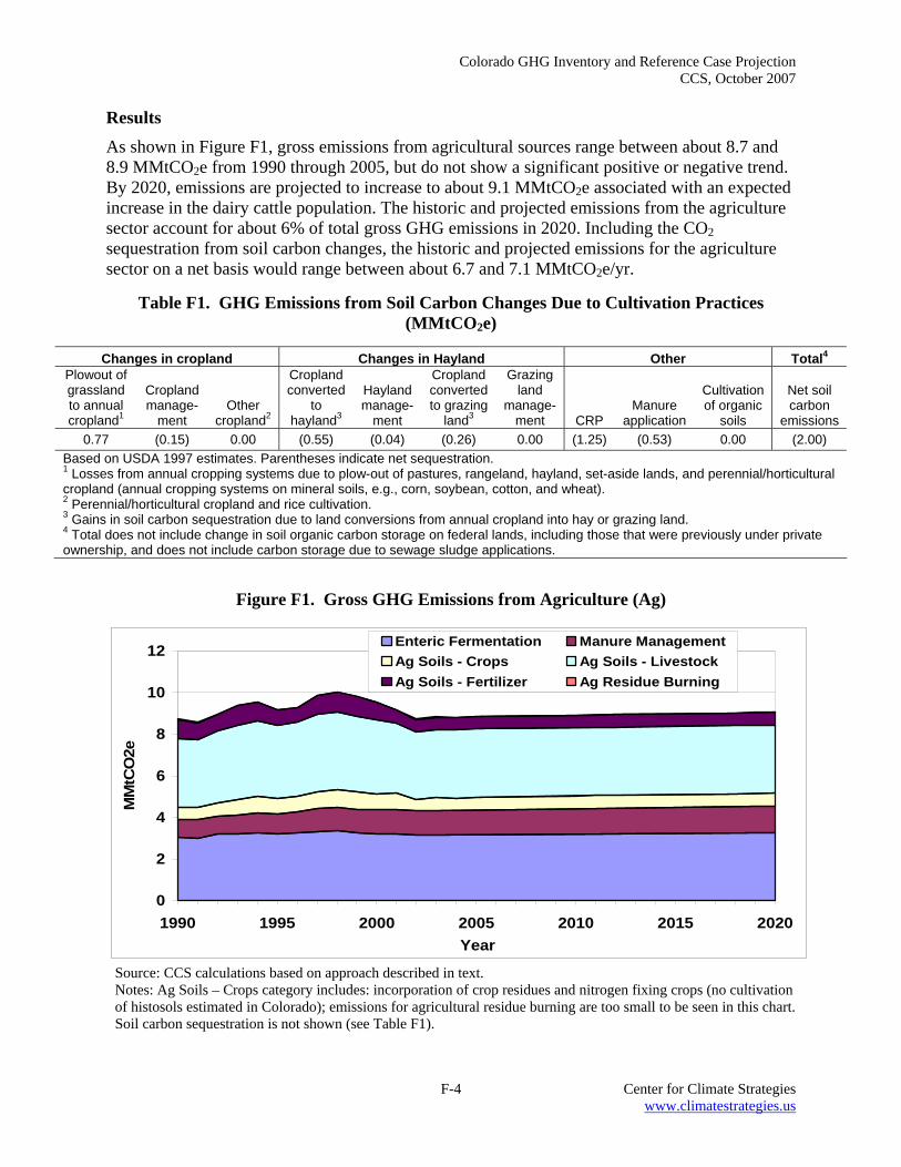
Colorado GHG Inventory and Reference Case Projection CCS, October 2007
F-4 Center for Climate Strategies www.climatestrategies.us
Results As shown in Figure F1, gross emissions from agricultural sources range between about 8.7 and 8.9 MMtCO2e from 1990 through 2005, but do not show a significant positive or negative trend. By 2020, emissions are projected to increase to about 9.1 MMtCO2e associated with an expected increase in the dairy cattle population. The historic and projected emissions from the agriculture sector account for about 6% of total gross GHG emissions in 2020. Including the CO2 sequestration from soil carbon changes, the historic and projected emissions for the agriculture sector on a net basis would range between about 6.7 and 7.1 MMtCO2e/yr.
Table F1. GHG Emissions from Soil Carbon Changes Due to Cultivation Practices (MMtCO2e)
Changes in cropland Changes in Hayland Other Total4 Plowout of grassland to annual cropland1
Cropland manage-
ment Other
cropland2
Cropland converted
to hayland3
Hayland manage-
ment
Cropland converted to grazing
land3
Grazing land
manage-ment CRP
Manure application
Cultivation of organic
soils
Net soil carbon
emissions 0.77 (0.15) 0.00 (0.55) (0.04) (0.26) 0.00 (1.25) (0.53) 0.00 (2.00)
Based on USDA 1997 estimates. Parentheses indicate net sequestration. 1 Losses from annual cropping systems due to plow-out of pastures, rangeland, hayland, set-aside lands, and perennial/horticultural cropland (annual cropping systems on mineral soils, e.g., corn, soybean, cotton, and wheat). 2 Perennial/horticultural cropland and rice cultivation. 3 Gains in soil carbon sequestration due to land conversions from annual cropland into hay or grazing land. 4 Total does not include change in soil organic carbon storage on federal lands, including those that were previously under private ownership, and does not include carbon storage due to sewage sludge applications.
Figure F1. Gross GHG Emissions from Agriculture (Ag)
0
2
4
6
8
10
12
1990 1995 2000 2005 2010 2015 2020Year
MM
tCO
2e
Enteric Fermentation Manure ManagementAg Soils - Crops Ag Soils - LivestockAg Soils - Fertilizer Ag Residue Burning
Source: CCS calculations based on approach described in text. Notes: Ag Soils – Crops category includes: incorporation of crop residues and nitrogen fixing crops (no cultivation of histosols estimated in Colorado); emissions for agricultural residue burning are too small to be seen in this chart. Soil carbon sequestration is not shown (see Table F1).
Colorado GHG Inventory and Reference Case Projection CCS, October 2007
F-5 Center for Climate Strategies www.climatestrategies.us
Agricultural burning emissions were estimated to be very small based on the SGIT activity data (<0.01 MMtCO2e/yr from 1990 to 2002). This agrees with the USDA Inventory which also reports a low level of residue burning emissions (0.02 MMtCO2e). The only standard IPCC source categories missing from this report are N2O emissions from cultivation of histosols and CO2 emissions from limestone and dolomite application. Estimates for Colorado were not available; however the USDA’s national estimate for soil liming is about 9 MMtCO2e/yr.125 Key Uncertainties Emissions from enteric fermentation and manure management are dependent on the estimates of animal populations and the various factors used to estimate emissions for each animal type and manure management system (i.e., emission factors that are dependent on several variables, including manure production levels, volatile solids contents of manures, and CH4 formation potential). Each of these factors has some level of uncertainty. Also, animal populations fluctuate throughout the year, and thus using point estimates introduces uncertainty into the average annual estimates of these populations. In addition, there is uncertainty associated with the original population survey methods employed by USDA. The largest contributors to uncertainty in emissions from manure management are the emission factors, which are derived from limited data sets. As mentioned above, for emissions associated with changes in agricultural soil carbon levels, the only data currently available are for 1997. When newer data are released by the USDA, these should be reviewed to represent current conditions as well as to assess trends. In particular, given the potential for some CRP acreage to retire and possibly return to active cultivation prior to 2020, the current size of the CO2 sink could be appreciably affected. As mentioned above, emission estimates for soil liming have not been developed for Colorado. Another contributor to uncertainty in the emission estimates is the projection assumptions. This inventory assumes that the dairy cattle population will grow at the historical rate. This population could, however level off or begin to decline before 2020, due to factors such as competition for water and feed.
125 U.S. Agriculture and Forestry Greenhouse Gas Inventory: 1990-2001. Global Change Program Office, Office of the Chief Economist, US Department of Agriculture.
Colorado GHG Inventory and Reference Case Projection CCS, October 2007
G-1 Center for Climate Strategies www.climatestrategies.us
Appendix G. Waste Management Overview GHG emissions from waste management include emissions from:
• Solid waste management – methane (CH4) emissions from municipal and industrial solid waste landfills (LFs), accounting for CH4 that is flared or captured for energy production (this includes both open and closed landfills);
• Solid waste combustion – CH4, carbon dioxide (CO2), and nitrous oxide (N2O) emissions from the combustion of solid waste in incinerators or waste to energy plants; and
• Wastewater management – CH4 and N2O from municipal wastewater and CH4 from industrial wastewater (WW) treatment facilities.
Waste management activities accounted for about 2% of Colorado’s gross GHG emissions in 2005.
Inventory and Reference Case Projections
Solid Waste Management For solid waste management, we used the US EPA SGIT software and the US EPA Landfill Methane Outreach Program (LMOP) landfills database126 as starting points to estimate emissions. The LMOP data serve as input data to estimate annual waste emplacement for each landfill modeled by SGIT. SGIT then estimates CH4 generation for each landfill site. Additional post-processing outside of SGIT to account for controls is then performed to estimate final CH4 emissions. The LMOP database was shared with CDPHE solid waste staff, and CCS was supplied with additional data on Colorado landfills. These additional data included information on many sites that were not present in the LMOP database, as well as updated information on sites that were present in the database (e.g. waste emplacement data, information on controls).127 In the combined LMOP and CDPHE dataset for Colorado, there are over 70 sites represented (both open and closed landfills). Small uncontrolled landfills in some counties were combined for the purposes of emissions modeling. Two of these sites collect landfill gas for use in a landfill gas to energy (LFGTE) plant. Another six sites collect and flare landfill gas. These eight sites are listed in the Table G1. The rest of the sites were assumed to be uncontrolled. To obtain the annual waste emplacement rate needed by SGIT for each landfill, the waste-in-place estimate was divided by the number of years of operation. This average annual disposal rate for each landfill was assumed for all years that the landfill was operating. For sites where the years of operation were not available, CCS estimated these years based on the waste-in-place estimate divided by the latest (2006) annual emplacement rate (note that for 2006, CDPHE stated 126 LMOP database is available at: http://www.epa.gov/lmop/proj/index.htm. Updated version of the database provided by Rachel Goldstein, Program Manager, EPA Landfill Methane Outreach Program, October 2006. 127 Charles Johnson, CDPHE, Solid Waste Division, personal communication and electronic data provided to S. Roe, CCS, December 2006.
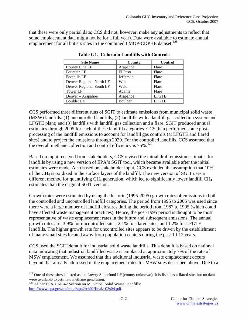
Colorado GHG Inventory and Reference Case Projection CCS, October 2007
G-2 Center for Climate Strategies www.climatestrategies.us
that these were only partial data; CCS did not, however, make any adjustments to reflect that some emplacement data might not be for a full year). Data were available to estimate annual emplacement for all but six sites in the combined LMOP-CDPHE dataset.128
Table G1. Colorado Landfills with Controls Site Name County Control
County Line LF Arapahoe Flare Fountain LF El Paso Flare Foothills LF Jefferson Flare Denver Regional North LF Weld Flare Denver Regional South LF Weld Flare Tower LF Adams Flare Denver – Arapahoe Arapahoe LFGTE Boulder LF Boulder LFGTE
CCS performed three different runs of SGIT to estimate emissions from municipal solid waste (MSW) landfills: (1) uncontrolled landfills; (2) landfills with a landfill gas collection system and LFGTE plant; and (3) landfills with landfill gas collection and a flare. SGIT produced annual estimates through 2005 for each of these landfill categories. CCS then performed some post-processing of the landfill emissions to account for landfill gas controls (at LFGTE and flared sites) and to project the emissions through 2020. For the controlled landfills, CCS assumed that the overall methane collection and control efficiency is 75%.129 Based on input received from stakeholders, CCS revised the initial draft emission estimates for landfills by using a new version of EPA’s SGIT tool, which became available after the initial estimates were made. Also based on stakeholder input, CCS excluded the assumption that 10% of the CH4 is oxidized in the surface layers of the landfill. The new version of SGIT uses a different method for quantifying CH4 generation, which led to significantly lower landfill CH4 estimates than the original SGIT version. Growth rates were estimated by using the historic (1995-2005) growth rates of emissions in both the controlled and uncontrolled landfill categories. The period from 1995 to 2005 was used since there were a large number of landfill closures during the period from 1987 to 1995 (which could have affected waste management practices). Hence, the post-1995 period is thought to be most representative of waste emplacement rates in the future and subsequent emissions. The annual growth rates are: 3.9% for uncontrolled sites; 2.1% for flared sites; and 1.2% for LFGTE landfills. The higher growth rate for uncontrolled sites appears to be driven by the establishment of many small sites located away from population centers during the past 10-12 years. CCS used the SGIT default for industrial solid waste landfills. This default is based on national data indicating that industrial landfilled waste is emplaced at approximately 7% of the rate of MSW emplacement. We assumed that this additional industrial waste emplacement occurs beyond that already addressed in the emplacement rates for MSW sites described above. Due to a 128 One of these sites is listed as the Lowry Superfund LF (county unknown). It is listed as a flared site, but no data were available to estimate methane generation. 129 As per EPA’s AP-42 Section on Municipal Solid Waste Landfills: http://www.epa.gov/ttn/chief/ap42/ch02/final/c02s04.pdf.

Colorado GHG Inventory and Reference Case Projection CCS, October 2007
G-3 Center for Climate Strategies www.climatestrategies.us
lack of data, no controls were assumed to be used on industrial waste landfills in Colorado. For industrial landfills, the overall growth rate in MSW emissions from 1995 to 2005 (2.6%/yr) was used to project emissions to 2010 and 2020 (based on the assumption that industrial waste landfilling will continue to grow at the same rate as MSW landfilling overall). Solid Waste Combustion CDPHE staff indicated that little to no municipal solid waste combustion has occurred during the 1990 – 2005 time-frame.130 This was true for both combustion in municipal solid waste combustors and open burning of municipal solid waste by Colorado residents. Hence, emissions for both the inventory and forecast for this sector are estimated to be negligible. Wastewater Management GHG emissions from municipal and industrial wastewater treatment were also estimated. For municipal wastewater treatment, emissions are calculated in EPA’s SGIT based on state population, assumed biochemical oxygen demand (BOD) and protein consumption per capita, and emission factors for N2O and CH4 from wastewater treatment The key SGIT default values are shown in Table G2. For industrial wastewater emissions, SGIT provides default assumptions and emission factors for three industrial sectors: Fruits & Vegetables, Red Meat & Poultry, and Pulp & Paper. CDPHE provided information on flows for the meat and poultry sector.131 Emissions from wastewater treatment for the other two industrial sectors are assumed to be negligible. The emissions were held constant at the 2005 level for the forecast years. This is because the data showed no significant growth in activity since the late 1990s and a reduction in activity in 2005.
Table G2. SGIT Key Default Values for Municipal Wastewater Treatment Variable Value
BOD 0.065 kg /day-person Amount of BOD anaerobically treated 16.25% CH4 emission factor 0.6 kg/kg BOD Colorado residents not on septic 75%
Water treatment N2O emission factor 4.0 g N20/person-yr Biosolids emission Factor 0.01 kg N2O-N/kg sewage-N Source: US EPA State Inventory Tool – Wastewater Module; methodology and factors taken from US EPA, Emission Inventory Improvement Program, Volume 8, Chapter 12, October 1999: www.epa.gov/ttn/chief/eiip/techreport/volume08/.
Figure G1 shows the emission estimates for the waste management sector. Overall, the sector accounts for 2.1 MMtCO2e in 2005. By 2020, emissions are expected to grow to 3.5 MMtCO2e/yr. The growth in emissions is driven largely by the solid waste management sector, in particular uncontrolled landfills. In 2005, about 48% of the emissions were contributed by the 130 Matt Burgett and Dale Wells, CDPHE, personal communications with S. Roe, CCS, January 2007. 131 Leslie Simpson, CDPHE, personal communication with S. Roe, CCS, November 2006 and electronic data on industrial wastewater flows. Data for two plants were provided (Cargill Meat Solutions, and Swift Beef). The total flows for these facilities in each year were used to estimate the amount of meat processed using the SGIT default of 13 cubic meters/Mt processed. The estimated production values were then used within SGIT to estimate methane emissions. Process wastewater flow data were available for 1990-2005.
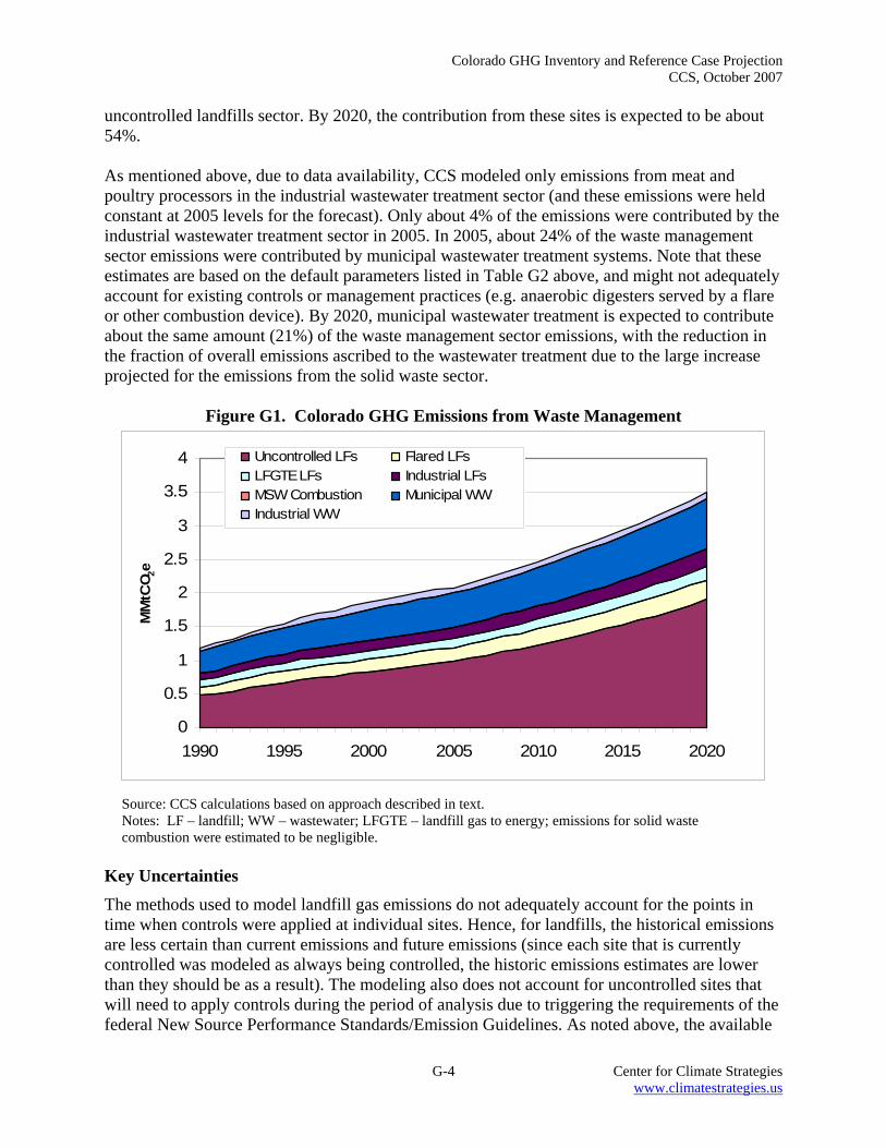
Colorado GHG Inventory and Reference Case Projection CCS, October 2007
G-4 Center for Climate Strategies www.climatestrategies.us
uncontrolled landfills sector. By 2020, the contribution from these sites is expected to be about 54%. As mentioned above, due to data availability, CCS modeled only emissions from meat and poultry processors in the industrial wastewater treatment sector (and these emissions were held constant at 2005 levels for the forecast). Only about 4% of the emissions were contributed by the industrial wastewater treatment sector in 2005. In 2005, about 24% of the waste management sector emissions were contributed by municipal wastewater treatment systems. Note that these estimates are based on the default parameters listed in Table G2 above, and might not adequately account for existing controls or management practices (e.g. anaerobic digesters served by a flare or other combustion device). By 2020, municipal wastewater treatment is expected to contribute about the same amount (21%) of the waste management sector emissions, with the reduction in the fraction of overall emissions ascribed to the wastewater treatment due to the large increase projected for the emissions from the solid waste sector.
Figure G1. Colorado GHG Emissions from Waste Management
0
0.5
1
1.5
2
2.5
3
3.5
4
1990 1995 2000 2005 2010 2015 2020
MM
tCO 2
e
Uncontrolled LFs Flared LFsLFGTE LFs Industrial LFsMSW Combustion Municipal WWIndustrial WW
Source: CCS calculations based on approach described in text. Notes: LF – landfill; WW – wastewater; LFGTE – landfill gas to energy; emissions for solid waste combustion were estimated to be negligible.
Key Uncertainties The methods used to model landfill gas emissions do not adequately account for the points in time when controls were applied at individual sites. Hence, for landfills, the historical emissions are less certain than current emissions and future emissions (since each site that is currently controlled was modeled as always being controlled, the historic emissions estimates are lower than they should be as a result). The modeling also does not account for uncontrolled sites that will need to apply controls during the period of analysis due to triggering the requirements of the federal New Source Performance Standards/Emission Guidelines. As noted above, the available

Colorado GHG Inventory and Reference Case Projection CCS, October 2007
G-5 Center for Climate Strategies www.climatestrategies.us
data do not cover all of the open and closed landfills in Colorado. For this reason, emissions could be slightly underestimated for landfills. For industrial landfills, emissions were estimated using national defaults (with industrial landfill wastes buried at 7% of the rate of MSW emplacement). It could be that the available MSW emplacement data within the combined LMOP data used to model the MSW emissions already captures industrial LF emplacement. As with overall MSW landfill emissions, industrial landfill emissions are projected to increase between 2005 and 2020. Hence, the industrial landfill inventory and forecast has a significant level of uncertainty and should be investigated further. For example, the existence of active industrial landfills that are not already represented in the LMOP database should be determined. If these sites do not exist and the existing municipal waste emplacement data are thought to include industrial wastes, then the separate estimate for industrial landfill emissions can be excluded from the inventory. For the wastewater sector, the key uncertainties are associated with the application of SGIT default values for the parameters listed in Table G2 above (e.g. the fraction of the Colorado population on septic sewers; and the fraction of BOD that is anaerobically decomposed). The SGIT defaults for emission factors used to estimate wastewater emissions were derived from national data.
Colorado GHG Inventory and Reference Case Projection CCS, October 2007
H-1 Center for Climate Strategies www.climatestrategies.us
Appendix H. Forestry Overview Forestland emissions refer to the net carbon dioxide (CO2) flux132 from forested lands in Colorado, which account for about 34% of the state’s land area.133 Forestlands are net sinks of CO2 in Colorado. Through photosynthesis, CO2 is taken up by trees and plants and converted to carbon in biomass within the forests. CO2 emissions occur from respiration in live trees and decay of dead biomass. In addition, carbon is stored for long time periods when forest biomass is harvested for use in durable wood products. CO2 flux is the net balance of CO2 removals from and emissions to the atmosphere from the processes described above. Inventory and Reference Case Projections For over a decade, the United State Forest Service (USFS) has been developing and refining a forest carbon modeling system for the purposes of estimating forest carbon inventories. The methodology is used to develop national forest CO2 fluxes for the official U.S. Inventory of Greenhouse Gas Emissions and Sinks.134 The national estimates are compiled from state-level data. The Colorado forest CO2 flux data in this report come from the national analysis and are provided by the USFS. The forest CO2 flux methodology relies on input data in the form of plot-level forest volume statistics from the Forest Inventory Analysis (FIA). FIA data on forest volumes are converted to values for ecosystem carbon stocks (i.e., the amount of carbon stored in forest carbon pools) using the FORCARB2 modeling system. Coefficients from FORCARB2 are applied to the plot level survey data to give estimates of carbon density (megagrams of C per hectare) for a number of separate carbon pools. CO2 flux is estimated as the change in carbon mass for each carbon pool over a specified time frame. Forest volume data from at least two points in time are required. The change in carbon stocks between time intervals is estimated at the plot level for specific carbon pools (Live Tree, Standing Dead Wood, Under-story, Down & Dead Wood, Forest Floor, and Soil Organic Carbon) and divided by the number of years between inventory samples. Annual increases in carbon density reflect carbon sequestration in a specific pool; decreases in carbon density reveal CO2 emissions or carbon transfers out of that pool (e.g., death of a standing tree transfers carbon from the live tree to standing dead wood pool). The amount of carbon in each pool is also influenced by changes in forest area (e.g., an increase in area could lead to an increase in the associated forest carbon pools and the estimated flux). The sum of carbon stock changes for all forest carbon pools yields a total net CO2 flux for forest ecosystems.
132 “Flux” refers to both emissions of CO2 to the atmosphere and removal (sinks) of CO2 from the atmosphere. 133 2001 Report on the Condition of Colorado’s Forests, Colorado Forestry Advisory Board, http://csfs.colostate.edu/library/pdfs/fhr/01fhr.pdf, reports 22.6 million acres of forested lands. The total land area in CO is 66.4 million acres (http://www.netstate.com/states/geography/co_geography.htm). 134 U.S. Inventory of Greenhouse Gas Emissions and Sinks: 1990-2004 (and earlier editions), US Environmental Protection Agency, Report # 430-R-06-002, April 2006. Available at: http://www.epa.gov/climatechange/emissions/usinventoryreport.html

Colorado GHG Inventory and Reference Case Projection CCS, October 2007
H-2 Center for Climate Strategies www.climatestrategies.us
In preparing these estimates, USFS estimates the amount of forest carbon in different forest types and as well as in different carbon pools. The different forests include those in the national forest system and those that are not federally-owned (private and other public forests). USFS also provides information on forests categorized as being either woodlands (forests with low productivity) and non-woodlands (e.g. timberlands or productive forest systems). Carbon pool data for two periods are used to estimate CO2 flux for each pool. The data shown in Table H1 are a summary of the FIA data used to derive the carbon pool and flux estimates that are summarized in Table H2. As shown in Table H1, the current forest carbon pool estimates are derived from 2004 FIA data. The previous inventory data came from either a previous FIA cycle or data from the Resources Planning Act Assessment (RPA). The Resources Planning Act requires the USFS to report on the state of US forest resources on a regular basis; the USFS publishes the RPA assessment every five years. FIA is a key contributor to RPA. RPA data, which are generally lower in resolution, are sometimes used in place of FIA cycles. The FIA has transitioned from a periodic to annual sampling design, which has created some forest inventory data sets that are not comparable over time, in which case the RPA data are better suited for estimating carbon densities.135 Except for the National Forests – Woodlands category, the interval between the current and previous surveys is around 22 years (early 1980s to 2004; data from the 1997 RPA report are from the early 1980s (the report contains a time series dating back to the 1950s).
Table H1. Forestry Data Used to Estimate Forest CO2 Flux
Forest Past Inventory
Source1 Avg. Year2
Interval3 (yr)
Current Forest Area
(103 hectares)
Previous Forest Area
(103 hectares)
National Forests – Non-Woodlands RPAdata_CO_1997 2004.2 22.9 4,219 4,020
National Forests – Woodlands FISDB21_CO_01_1984 2004.3 6.9 366 174
Non-National Forests – Non-Woodlands FIADBWW_CO_1983 2004.2 23.7 2,067 1,975
Non-National Forests – Woodlands FIADBWW_CO_1983 2004.2 20.9 2,774 2,351
Totals 9,425 8,5191 Current Inventory Source for all groups was FISDB21_CO_02_2005. 2 Average year for the current FIA inventory data. 3 The number of years between the current inventory source and the past inventory source.
The data in Table H1 show an increase of 906 kilo-hectares (2.2 million acres) in forested area from the early-1980s through 2004. About two-thirds of this increase occurred in woodland forests (as mentioned under key uncertainties below, some of this difference is likely driven by methodological differences in survey methods).
135 Jim Smith, USFS, personal communication with K. Bickel, CCS, November 7, 2006.
Colorado GHG Inventory and Reference Case Projection CCS, October 2007
H-3 Center for Climate Strategies www.climatestrategies.us
Table H2 provides a summary of the size of the forest carbon pools for the final survey period and the resultant flux estimates (in units of carbon and CO2) developed by the USFS.3 A total of 31 million metric tons (MMt) CO2 is estimated to be sequestered in Colorado forests each year, with about half of this accumulating in the live tree carbon pool. The soil organic carbon and forest floor pools had the next largest accumulations of carbon at 7 and 5 MMtCO2/yr, respectively. Note that this analysis averages out annual fluctuations in carbon sequestration rates over an approximately 20-year time interval. In addition to the forest carbon pools, additional carbon stored as biomass is removed from the forest for the production of durable wood products; carbon remains stored in the products pool or is transferred to landfills where much of the carbon remains stored over long period of time. An estimated 0.8 MMt carbon dioxide equivalent (CO2e) is sequestered annually in wood products; these data are based on a USFS study from 1987 to 1997.136.Additional details on all of the forest carbon inventory methods can be found in Annex 3 to United States Environmental Protection Agency’s (EPA) 2006 GHG inventory for the US.137 Recent discussions with the USFS have indicated that there is considerable uncertainty with the soil organic carbon flux estimates. Due to this uncertainty, their recommendation is to leave this flux out of the statewide totals for carbon flux. In Table H2, a total forest flux which excludes the soil organic carbon pool has been provided (-24.7 MMtCO2), and this estimate has been used in the summary tables at the front of this report. For the 1990 and 2000 historic emission estimates, as well as the reference case projections, the forest area and carbon densities of forestlands were assumed to be at the same levels as those shown in Table H2. Hence, there is no change in the estimated future sinks for 2010 and 2020. These assumptions could change based on feedback from project stakeholders and other state forestry experts. In order to provide a more comprehensive understanding of GHG sources/sinks from the forestry sector, the Center for Climate Strategies (CCS) also developed some rough estimates of state-wide emissions for methane (CH4) and nitrous oxide (N2O) from wildfires and prescribed burns. A study published earlier this year in Science indicated an increasing frequency of wildfire activity in the western US driven by a longer fire season and higher temperatures.138
136 http://www.fs.fed.us/ne/global/pubs/books/epa/states. 137 Annex 3 to US EPA’s 2006 report can be downloaded at: http://yosemite.epa.gov/oar/globalwarming.nsf/UniqueKeyLookup/RAMR6MBLNQ/$File/06_annex_Chapter3.pdf. 138 Westerling, A.L. et al, “Warming and Earlier Spring Increases Western US Forest Wildfire Activity”, Sciencexpress, July 6, 2006.

Colorado GHG Inventory and Reference Case Projection CCS, October 2007
H-4 Center for Climate Strategies www.climatestrategies.us
Table H2. Forestry CO2 Flux Estimates for Colorado Carbon Pool (MMt Carbon)
Forest Live Tree Standing
Dead Under-story
Down & Dead
Forest Floor
Soil Organic Carbon
National Forests – Non-Woodlands 346.1 46.0 9.2 27.0 137.0 152.6 National Forests – Woodlands 9.0 0.4 1.5 0.4 9.0 11.4 Non-National Forests – Non-Woodlands 107.3 13.1 5.5 8.0 55.3 63.8 Non-National Forests – Woodlands 73.3 1.0 9.2 2.6 61.5 68.7
Totals 535.7 60.5 25.3 38.0 262.8 296.5
Carbon Pool Flux (MMt carbon/year)
Forest Live Tree Standing
Dead Under-story
Down & Dead
Forest Floor
Soil Organic Carbon
National Forests – Non-Woodlands -2.72 -0.32 -0.02 -0.20 -0.30 -0.43 National Forests – Woodlands -0.70 -0.03 -0.11 -0.03 -0.71 -0.88 Non-National Forests – Non-Woodlands -0.03 -0.02 -0.01 0.00 0.05 0.21 Non-National Forests – Woodlands -0.73 -0.02 -0.10 -0.03 -0.47 -0.82
Totals -4.18 -0.40 -0.24 -0.27 -1.42 -1.92
Carbon Pool Flux (MMt CO2/yr)
Forest
Live Tree Standing
Dead Under-story
Down & Dead
Forest Floor
Soil Organic Carbon
National Forests – Non-Woodlands -10.0 -1.2 -0.1 -0.7 -1.1 -1.6 National Forests – Woodlands -2.6 -0.1 -0.4 -0.1 -2.6 -3.2 Non-National Forests – Non-Woodlands -0.1 -0.1 0.0 0.0 0.2 0.8 Non-National Forests – Woodlands -2.7 -0.1 -0.4 -0.1 -1.7 -3.0
Totals -15.3 -1.5 -0.9 -1.0 -5.2 -7.1
Total Forest Flux = -30.9 Harvested Wood Products1 = -0.8
Total Statewide Flux = -31.8 Total Excluding Soil Organic
Carbon = -24.7 NOTE: Totals may not add exactly due to rounding. 1 Source: http://www.fs.fed.us/ne/global/pubs/books/epa/states; For Colorado, HWP are estimated to sequester 0.22 MMtC during the period 1987-1997).

Colorado GHG Inventory and Reference Case Projection CCS, October 2007
H-5 Center for Climate Strategies www.climatestrategies.us
CCS used 2002 emissions data developed by the Western Regional Air Partnership (WRAP) to estimate CO2e emissions for wildfires and prescribed burns.139 The CO2e from CH4 emissions from this study were added to an estimate of CO2e for N2O to estimate a total CO2e for fires (the CO2 emissions from fires are captured within the carbon pool accounting methods described above). The nitrous oxide estimate was made assuming that N2O was 1% of the emissions of nitrogen oxides (NOx) from the WRAP study. The 1% estimate is a common rule of thumb for the N2O content of NOx from combustion sources. CCS is soliciting feedback on this assumption. The results for 2002 are that fires contributed over 1.2 MMtCO2e of CH4 and NOx from about 511,000 acres burned (495,000 acres by wildfires). About 94% of the CO2e was contributed by CH4. Note that this level of activity compares to less than 90,000 acres burned in Colorado in 1996.140 Given the large swings in fire activity from year to year and the current lack of data for multiple years, CCS will discuss this issue with project stakeholders before including the fire emission estimates in the GHG inventory. Key Uncertainties It is important to note that there were methodological differences in the two FIA cycles that can produce different estimates of forested area and carbon density. In the Rocky Mountain Region, the FIA program modified the definition of forest cover for the woodlands class of forestland. Earlier FIA cycles defined woodlands as having a tree cover of at least 10%, while the newer sampling methods used a woodlands definition of tree cover of at least 5% (leading to more area being defined as woodland). In woodland areas, the earlier FIA surveys might not have inventoried trees of certain species or with certain tree form characteristics (leading to differences in both carbon density and forested acreage). Also, surveys since 1999 include all dead trees on the plots, but data prior to that are variable in terms of these data. The modifications to FIA surveys are a result of an expanded focus in the FIA program, which historically was only concerned with timber resources, while more recent surveys have aimed at a more comprehensive gathering of forest biomass data. The effect of these changes in survey methods has not been estimated by the USFS. In states like Colorado with significant areas of woodlands, the change in definition could contribute significantly to the increases seen in forested area in Colorado and the associated CO2 flux. For these reasons, the USFS provided flux estimates separately for woodlands and non-woodlands (i.e., all other forest classes), so that the relative influence of these classes on total net CO2 fluxes in Colorado could be discerned. As shown in Table H2, the contribution from the woodland areas drives a significant fraction of the flux estimate statewide. Given the differences in FIA survey methods, the forest flux estimates should be viewed as conservatively high for Colorado forests (i.e., more likely to have a higher than lower magnitude of CO2 flux into forest lands). As mentioned above, CCS included the forestry estimates without the soil carbon pool in the emissions summary tables (see Tables ES-1 and Table 1) for this report, since the USFS has indicated a high level of uncertainty for this carbon pool. These uncertainties are likely to remain until additional data from measurements and potentially improved modeling methods are developed. 139 2002 Fire Emission Inventory for the WRAP Region Phase I – Essential Documentation, prepared by Air Sciences, Inc., June 2004. 140 1996 Fire Emission Inventory, Draft Final Report, prepared by Air Sciences, Inc., December 2002.
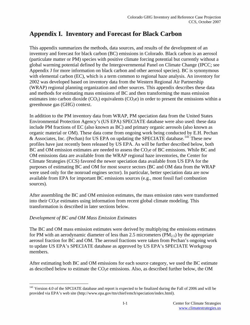
Colorado GHG Inventory and Reference Case Projection CCS, October 2007
I-1 Center for Climate Strategies www.climatestrategies.us
Appendix I. Inventory and Forecast for Black Carbon This appendix summarizes the methods, data sources, and results of the development of an inventory and forecast for black carbon (BC) emissions in Colorado. Black carbon is an aerosol (particulate matter or PM) species with positive climate forcing potential but currently without a global warming potential defined by the Intergovernmental Panel on Climate Change (IPCC; see Appendix J for more information on black carbon and other aerosol species). BC is synonymous with elemental carbon (EC), which is a term common to regional haze analysis. An inventory for 2002 was developed based on inventory data from the Western Regional Air Partnership (WRAP) regional planning organization and other sources. This appendix describes these data and methods for estimating mass emissions of BC and then transforming the mass emission estimates into carbon dioxide (CO2) equivalents (CO2e) in order to present the emissions within a greenhouse gas (GHG) context. In addition to the PM inventory data from WRAP, PM speciation data from the United States Environmental Protection Agency’s (US EPA) SPECIATE database were also used: these data include PM fractions of EC (also known as BC) and primary organic aerosols (also known as organic material or OM). These data come from ongoing work being conducted by E.H. Pechan & Associates, Inc. (Pechan) for US EPA on updating the SPECIATE database.141 These new profiles have just recently been released by US EPA. As will be further described below, both BC and OM emission estimates are needed to assess the CO2e of BC emissions. While BC and OM emissions data are available from the WRAP regional haze inventories, the Center for Climate Strategies (CCS) favored the newer speciation data available from US EPA for the purposes of estimating BC and OM for most source sectors (BC and OM data from the WRAP were used only for the nonroad engines sector). In particular, better speciation data are now available from EPA for important BC emissions sources (e.g., most fossil fuel combustion sources). After assembling the BC and OM emission estimates, the mass emission rates were transformed into their CO2e estimates using information from recent global climate modeling. This transformation is described in later sections below. Development of BC and OM Mass Emission Estimates The BC and OM mass emission estimates were derived by multiplying the emissions estimates for PM with an aerodynamic diameter of less than 2.5 micrometers (PM2.5) by the appropriate aerosol fraction for BC and OM. The aerosol fractions were taken from Pechan’s ongoing work to update US EPA’s SPECIATE database as approved by US EPA’s SPECIATE Workgroup members. After estimating both BC and OM emissions for each source category, we used the BC estimate as described below to estimate the CO2e emissions. Also, as described further below, the OM
141 Version 4.0 of the SPCIATE database and report is expected to be finalized during the Fall of 2006 and will be provided via EPA’s web site (http://www.epa.gov/ttn/chief/emch/speciation/index.html).
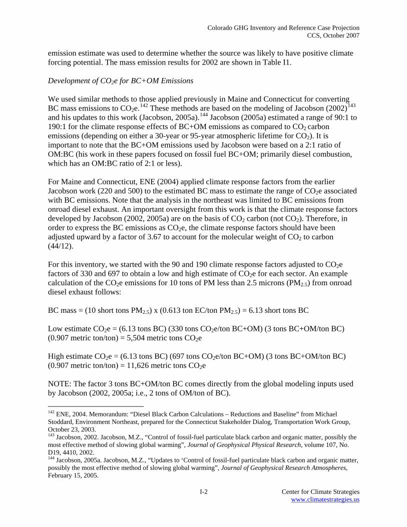
Colorado GHG Inventory and Reference Case Projection CCS, October 2007
I-2 Center for Climate Strategies www.climatestrategies.us
emission estimate was used to determine whether the source was likely to have positive climate forcing potential. The mass emission results for 2002 are shown in Table I1. Development of CO2e for BC+OM Emissions We used similar methods to those applied previously in Maine and Connecticut for converting BC mass emissions to CO2e.142 These methods are based on the modeling of Jacobson (2002)143 and his updates to this work (Jacobson, 2005a).144 Jacobson (2005a) estimated a range of 90:1 to 190:1 for the climate response effects of BC+OM emissions as compared to CO2 carbon emissions (depending on either a 30-year or 95-year atmospheric lifetime for CO2). It is important to note that the BC+OM emissions used by Jacobson were based on a 2:1 ratio of OM:BC (his work in these papers focused on fossil fuel BC+OM; primarily diesel combustion, which has an OM:BC ratio of 2:1 or less). For Maine and Connecticut, ENE (2004) applied climate response factors from the earlier Jacobson work (220 and 500) to the estimated BC mass to estimate the range of CO2e associated with BC emissions. Note that the analysis in the northeast was limited to BC emissions from onroad diesel exhaust. An important oversight from this work is that the climate response factors developed by Jacobson (2002, 2005a) are on the basis of CO2 carbon (not CO2). Therefore, in order to express the BC emissions as CO2e, the climate response factors should have been adjusted upward by a factor of 3.67 to account for the molecular weight of CO2 to carbon (44/12). For this inventory, we started with the 90 and 190 climate response factors adjusted to CO2e factors of 330 and 697 to obtain a low and high estimate of CO2e for each sector. An example calculation of the CO2e emissions for 10 tons of PM less than 2.5 microns (PM2.5) from onroad diesel exhaust follows: BC mass = (10 short tons PM2.5) x (0.613 ton EC/ton PM2.5) = 6.13 short tons BC Low estimate CO2e = (6.13 tons BC) (330 tons CO2e/ton BC+OM) (3 tons BC+OM/ton BC) (0.907 metric ton/ton) = 5,504 metric tons CO2e High estimate CO2e = (6.13 tons BC) (697 tons CO2e/ton BC+OM) (3 tons BC+OM/ton BC) (0.907 metric ton/ton) = 11,626 metric tons CO2e NOTE: The factor 3 tons BC+OM/ton BC comes directly from the global modeling inputs used by Jacobson (2002, 2005a; i.e., 2 tons of OM/ton of BC). 142 ENE, 2004. Memorandum: “Diesel Black Carbon Calculations – Reductions and Baseline” from Michael Stoddard, Environment Northeast, prepared for the Connecticut Stakeholder Dialog, Transportation Work Group, October 23, 2003. 143 Jacobson, 2002. Jacobson, M.Z., “Control of fossil-fuel particulate black carbon and organic matter, possibly the most effective method of slowing global warming”, Journal of Geophysical Physical Research, volume 107, No. D19, 4410, 2002. 144 Jacobson, 2005a. Jacobson, M.Z., “Updates to ‘Control of fossil-fuel particulate black carbon and organic matter, possibly the most effective method of slowing global warming”, Journal of Geophysical Research Atmospheres, February 15, 2005.
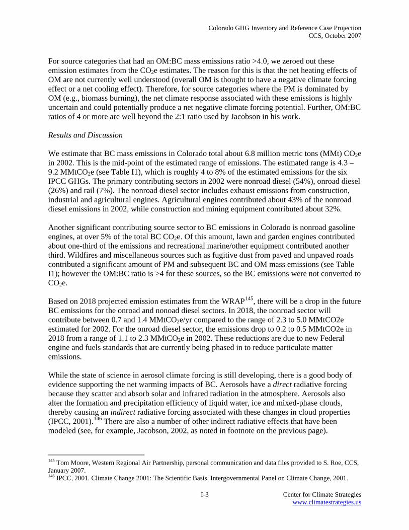
Colorado GHG Inventory and Reference Case Projection CCS, October 2007
I-3 Center for Climate Strategies www.climatestrategies.us
For source categories that had an OM:BC mass emissions ratio >4.0, we zeroed out these emission estimates from the CO2e estimates. The reason for this is that the net heating effects of OM are not currently well understood (overall OM is thought to have a negative climate forcing effect or a net cooling effect). Therefore, for source categories where the PM is dominated by OM (e.g., biomass burning), the net climate response associated with these emissions is highly uncertain and could potentially produce a net negative climate forcing potential. Further, OM:BC ratios of 4 or more are well beyond the 2:1 ratio used by Jacobson in his work. Results and Discussion We estimate that BC mass emissions in Colorado total about 6.8 million metric tons (MMt) CO2e in 2002. This is the mid-point of the estimated range of emissions. The estimated range is 4.3 – 9.2 MMtCO2e (see Table I1), which is roughly 4 to 8% of the estimated emissions for the six IPCC GHGs. The primary contributing sectors in 2002 were nonroad diesel (54%), onroad diesel (26%) and rail (7%). The nonroad diesel sector includes exhaust emissions from construction, industrial and agricultural engines. Agricultural engines contributed about 43% of the nonroad diesel emissions in 2002, while construction and mining equipment contributed about 32%. Another significant contributing source sector to BC emissions in Colorado is nonroad gasoline engines, at over 5% of the total BC CO2e. Of this amount, lawn and garden engines contributed about one-third of the emissions and recreational marine/other equipment contributed another third. Wildfires and miscellaneous sources such as fugitive dust from paved and unpaved roads contributed a significant amount of PM and subsequent BC and OM mass emissions (see Table I1); however the OM:BC ratio is >4 for these sources, so the BC emissions were not converted to CO2e. Based on 2018 projected emission estimates from the WRAP145, there will be a drop in the future BC emissions for the onroad and nonoad diesel sectors. In 2018, the nonroad sector will contribute between 0.7 and 1.4 MMtCO2e/yr compared to the range of 2.3 to 5.0 MMtCO2e estimated for 2002. For the onroad diesel sector, the emissions drop to 0.2 to 0.5 MMtCO2e in 2018 from a range of 1.1 to 2.3 MMtCO2e in 2002. These reductions are due to new Federal engine and fuels standards that are currently being phased in to reduce particulate matter emissions. While the state of science in aerosol climate forcing is still developing, there is a good body of evidence supporting the net warming impacts of BC. Aerosols have a direct radiative forcing because they scatter and absorb solar and infrared radiation in the atmosphere. Aerosols also alter the formation and precipitation efficiency of liquid water, ice and mixed-phase clouds, thereby causing an indirect radiative forcing associated with these changes in cloud properties (IPCC, 2001).146 There are also a number of other indirect radiative effects that have been modeled (see, for example, Jacobson, 2002, as noted in footnote on the previous page).
145 Tom Moore, Western Regional Air Partnership, personal communication and data files provided to S. Roe, CCS, January 2007. 146 IPCC, 2001. Climate Change 2001: The Scientific Basis, Intergovernmental Panel on Climate Change, 2001.
Colorado GHG Inventory and Reference Case Projection CCS, October 2007
I-4 Center for Climate Strategies www.climatestrategies.us
The quantification of aerosol radiative forcing is more complex than the quantification of radiative forcing by GHGs because of the direct and indirect radiative forcing effects, and the fact that aerosol mass and particle number concentrations are highly variable in space and time. This variability is largely due to the much shorter atmospheric lifetime of aerosols compared with the important GHGs (i.e., CO2). Spatially- and temporally-resolved information on the atmospheric concentration and radiative properties of aerosols is needed to estimate radiative forcing. The quantification of indirect radiative forcing by aerosols is especially difficult. In addition to the variability in aerosol concentrations, some complicated aerosol influences on cloud processes must be accurately modeled. For example, the warm (liquid water) cloud indirect forcing may be divided into two components. The first indirect forcing is associated with the change in droplet concentration caused by increases in aerosol cloud condensation nuclei. The second indirect forcing is associated with the change in precipitation efficiency that results from a change in droplet number concentration. Quantification of the latter forcing necessitates understanding of a change in cloud liquid-water content. In addition to warm clouds, ice clouds may also be affected by aerosols. To put the radiative forcing potential of BC in context with CO2, the IPCC estimated the radiative forcing for a doubling of the earth’s CO2 concentration to be 3.7 watts per square meter (W/m2). For BC, various estimates of current radiative forcing have ranged from 0.16 to 0.42 W/m2 (IPCC, 2001). These BC estimates are for direct radiative effects only. There is a higher level of uncertainty associated with the direct radiative forcing estimates of BC compared to those of CO2 and other GHGs. There are even higher uncertainties associated with the assessment of the indirect radiative forcing of aerosols.

Colorado GHG Inventory and Reference Case Projection CCS, October 2007
I-5 Center for Climate Strategies www.climatestrategies.us
Table I1. 2002 BC Emission Estimates
Mass Emissions CO2 Equivalents BC OM BC + OM Low High
Contribution to CO2e Sector Subsector
Metric Tons Metric Tons % Electricity Generating Units (EGUs) Coal 66 102 168 66,469 140,392 1.5% Oil 0 0 0 17,983 37,983 0.4% Gas 0 7 7 0 0 0.0% Other 19 243 262 503 1,063 0.0% Non-EGU Fuel Combustion (Residential, Commercial, and Industrial) Coal 11 239 250 43,678 92,253 1.0% Oil 25 13 39 32,620 68,898 0.8% Gas 0 300 300 0 0 0.0% Othera 1,563 8,337 9,900 2,391 5,049 0.1% Onroad Gasoline (Exhaust, Brake Wear, & Tire Wear) 168 664 832 63,315 133,728 1.5% Onroad Diesel (Exhaust, Brake Wear, & Tire Wear) 1,250 522 1,772 1,113,198 2,351,209 25.6% Aircraft 93 156 249 92,119 194,567 2.1% Railroadb 320 105 426 317,249 670,068 7.3% Other Energy Use Nonroad Gas 212 596 807 209,402 442,283 4.8% Nonroad Diesel 2,375 779 3,154 2,350,832 4,965,242 54.1% Other Combustionc 3 0 3 0 0 0.0% Industrial Processes 87 0 87 32,917 69,526 0.8% Agricultured 324 0 324 0 0 0.0% Waste Management Landfills 1 473 474 0 0 0.0% Incineration 1 0 1 692 1,462 0.0% Open Burning 0 0 1 190 402 0.0% Other 4 80 84 0 0 0.0% Wildfires/Prescribed Burns 6,652 66,543 73,196 0 0 0.0% Miscellaneouse 321 5,317 5,638 0 0 0.0%
Totals 13,496 84,478 97,974 4,343,559 9,174,123 100% a Primarily wood-fired commercial/industrial boilers with some large diesel engines. b Railroad includes Locomotives and Railroad Equipment Emissions. c Other Combustion includes Motor Vehicle Fire, Structure Fire, and Aircraft/Rocket Engine Fire & Testing Emissions. d Agriculture includes Agricultural Burning, Agriculture/Forestry and Agriculture, Food, & Kindred Spirits Emissions. e Miscellaneous includes Paved/Unpaved Roads and Catastrophic/Accidental Release Emissions.

Colorado GHG Inventory and Reference Case Projection CCS, October 2007
J-1 Center for Climate Strategies www.climatestrategies.us
Appendix J. Greenhouse Gases and Global Warming Potential Values: Excerpts from the Inventory of U.S. Greenhouse Emissions and Sinks: 1990-2000 Original Reference: Material for this Appendix is taken from the Inventory of U.S. Greenhouse Gas Emissions and Sinks: 1990 - 2000, U.S. Environmental Protection Agency, Office of Atmospheric Programs, EPA 430-R-02-003, April 2002 www.epa.gov/globalwarming/publications/emissions Michael Gillenwater directed the preparation of this appendix. Introduction The Inventory of U.S. Greenhouse Gas Emissions and Sinks presents estimates by the United States government of U.S. anthropogenic greenhouse gas emissions and removals for the years 1990 through 2000. The estimates are presented on both a full molecular mass basis and on a Global Warming Potential (GWP) weighted basis in order to show the relative contribution of each gas to global average radiative forcing.
The Intergovernmental Panel on Climate Change (IPCC) has recently updated the specific global warming potentials for most greenhouse gases in their Third Assessment Report (TAR, IPCC 2001). Although the GWPs have been updated, estimates of emissions presented in the U.S. Inventory continue to use the GWPs from the Second Assessment Report (SAR). The guidelines under which the Inventory is developed, the Revised 1996 IPCC Guidelines for National Greenhouse Gas Inventories (IPCC/UNEP/OECD/IEA 1997) and the United Nations Framework Convention on Climate Change (UNFCCC) reporting guidelines for national inventories147 were developed prior to the publication of the TAR. Therefore, to comply with international reporting standards under the UNFCCC, official emission estimates are reported by the United States using SAR GWP values. This excerpt of the U.S. Inventory addresses in detail the differences between emission estimates using these two sets of GWPs. Overall, these revisions to GWP values do not have a significant effect on U.S. emission trends.
Additional discussion on emission trends for the United States can be found in the complete Inventory of U.S. Greenhouse Gas Emissions and Sinks: 1990-2000.
What is Climate Change? Climate change refers to long-term fluctuations in temperature, precipitation, wind, and other elements of the Earth’s climate system. Natural processes such as solar-irradiance variations, variations in the Earth’s orbital parameters, and volcanic activity can produce variations in climate. The climate system can also be influenced by changes in the concentration of various gases in the atmosphere, which affect the Earth’s absorption of radiation.
The Earth naturally absorbs and reflects incoming solar radiation and emits longer wavelength terrestrial (thermal) radiation back into space. On average, the absorbed solar radiation is balanced by the outgoing terrestrial radiation emitted to space. A portion of this terrestrial radiation, though, is itself absorbed by gases in the atmosphere. The energy from this absorbed terrestrial radiation warms the Earth's surface and atmosphere, creating what is known as the “natural greenhouse effect.” Without the natural heat-trapping properties of these atmospheric gases, the average surface temperature of the Earth would be about 33oC lower (IPCC 2001). 147 See FCCC/CP/1999/7 at www.unfccc.de
Colorado GHG Inventory and Reference Case Projection CCS, October 2007
J-2 Center for Climate Strategies www.climatestrategies.us
Under the UNFCCC, the definition of climate change is “a change of climate which is attributed directly or indirectly to human activity that alters the composition of the global atmosphere and which is in addition to natural climate variability observed over comparable time periods.” Given that definition, in its Second Assessment Report of the science of climate change, the IPCC concluded that:
Human activities are changing the atmospheric concentrations and distributions of greenhouse gases and aerosols. These changes can produce a radiative forcing by changing either the reflection or absorption of solar radiation, or the emission and absorption of terrestrial radiation (IPCC 1996).
Building on that conclusion, the more recent IPCC Third Assessment Report asserts that “[c]oncentrations of atmospheric greenhouse gases and their radiative forcing have continued to increase as a result of human activities” (IPCC 2001).
The IPCC went on to report that the global average surface temperature of the Earth has increased by between 0.6 ± 0.2°C over the 20th century (IPCC 2001). This value is about 0.15°C larger than that estimated by the Second Assessment Report, which reported for the period up to 1994, “owing to the relatively high temperatures of the additional years (1995 to 2000) and improved methods of processing the data” (IPCC 2001).
While the Second Assessment Report concluded, “the balance of evidence suggests that there is a discernible human influence on global climate,” the Third Assessment Report states the influence of human activities on climate in even starker terms. It concludes that, “[I]n light of new evidence and taking into account the remaining uncertainties, most of the observed warming over the last 50 years is likely to have been due to the increase in greenhouse gas concentrations” (IPCC 2001).
Greenhouse Gases Although the Earth’s atmosphere consists mainly of oxygen and nitrogen, neither plays a significant role in enhancing the greenhouse effect because both are essentially transparent to terrestrial radiation. The greenhouse effect is primarily a function of the concentration of water vapor, carbon dioxide, and other trace gases in the atmosphere that absorb the terrestrial radiation leaving the surface of the Earth (IPCC 1996). Changes in the atmospheric concentrations of these greenhouse gases can alter the balance of energy transfers between the atmosphere, space, land, and the oceans. A gauge of these changes is called radiative forcing, which is a simple measure of changes in the energy available to the Earth-atmosphere system (IPCC 1996). Holding everything else constant, increases in greenhouse gas concentrations in the atmosphere will produce positive radiative forcing (i.e., a net increase in the absorption of energy by the Earth).
Climate change can be driven by changes in the atmospheric concentrations of a number of radiatively active gases and aerosols. We have clear evidence that human activities have affected concentrations, distributions and life cycles of these gases (IPCC 1996).
Naturally occurring greenhouse gases include water vapor, carbon dioxide (CO2), methane (CH4), nitrous oxide (N2O), and ozone (O3). Several classes of halogenated substances that contain fluorine, chlorine, or bromine are also greenhouse gases, but they are, for the most part, solely a product of industrial activities. Chlorofluorocarbons (CFCs) and hydrochlorofluorocarbons (HCFCs) are halocarbons that contain chlorine, while halocarbons that contain bromine are referred to as bromofluorocarbons (i.e., halons). Because CFCs, HCFCs, and
Colorado GHG Inventory and Reference Case Projection CCS, October 2007
J-3 Center for Climate Strategies www.climatestrategies.us
halons are stratospheric ozone depleting substances, they are covered under the Montreal Protocol on Substances that Deplete the Ozone Layer. The UNFCCC defers to this earlier international treaty; consequently these gases are not included in national greenhouse gas inventories. Some other fluorine containing halogenated substances—hydrofluorocarbons (HFCs), perfluorocarbons (PFCs), and sulfur hexafluoride (SF6)—do not deplete stratospheric ozone but are potent greenhouse gases. These latter substances are addressed by the UNFCCC and accounted for in national greenhouse gas inventories.
There are also several gases that, although they do not have a commonly agreed upon direct radiative forcing effect, do influence the global radiation budget. These tropospheric gases—referred to as ambient air pollutants—include carbon monoxide (CO), nitrogen dioxide (NO2), sulfur dioxide (SO2), and tropospheric (ground level) ozone (O3). Tropospheric ozone is formed by two precursor pollutants, volatile organic compounds (VOCs) and nitrogen oxides (NOx) in the presence of ultraviolet light (sunlight). Aerosols—extremely small particles or liquid droplets—often composed of sulfur compounds, carbonaceous combustion products, crustal materials and other human induced pollutants—can affect the absorptive characteristics of the atmosphere. However, the level of scientific understanding of aerosols is still very low (IPCC 2001).
Carbon dioxide, methane, and nitrous oxide are continuously emitted to and removed from the atmosphere by natural processes on Earth. Anthropogenic activities, however, can cause additional quantities of these and other greenhouse gases to be emitted or sequestered, thereby changing their global average atmospheric concentrations. Natural activities such as respiration by plants or animals and seasonal cycles of plant growth and decay are examples of processes that only cycle carbon or nitrogen between the atmosphere and organic biomass. Such processes—except when directly or indirectly perturbed out of equilibrium by anthropogenic activities—generally do not alter average atmospheric greenhouse gas concentrations over decadal timeframes. Climatic changes resulting from anthropogenic activities, however, could have positive or negative feedback effects on these natural systems. Atmospheric concentrations of these gases, along with their rates of growth and atmospheric lifetimes, are presented in Table 10.
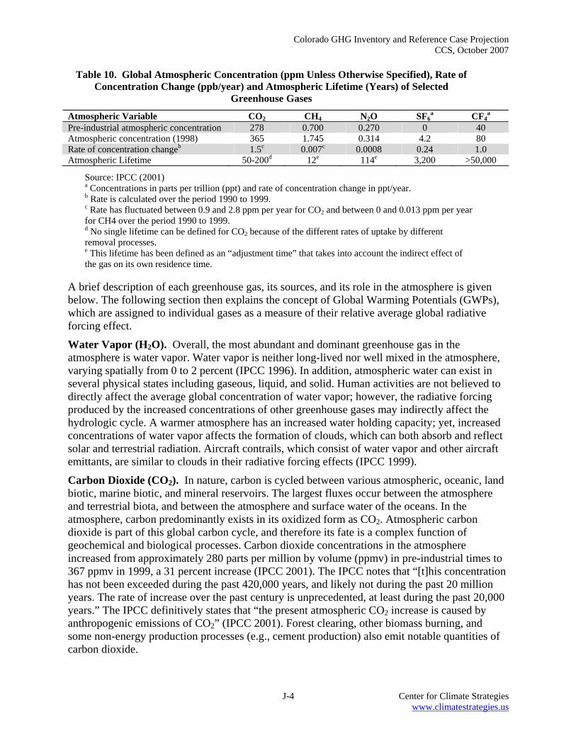
Colorado GHG Inventory and Reference Case Projection CCS, October 2007
J-4 Center for Climate Strategies www.climatestrategies.us
Table 10. Global Atmospheric Concentration (ppm Unless Otherwise Specified), Rate of Concentration Change (ppb/year) and Atmospheric Lifetime (Years) of Selected
Greenhouse Gases
Atmospheric Variable CO2 CH4 N2O SF6a CF4
a Pre-industrial atmospheric concentration 278 0.700 0.270 0 40 Atmospheric concentration (1998) 365 1.745 0.314 4.2 80 Rate of concentration changeb 1.5c 0.007c 0.0008 0.24 1.0 Atmospheric Lifetime 50-200d 12e 114e 3,200 >50,000
Source: IPCC (2001) a Concentrations in parts per trillion (ppt) and rate of concentration change in ppt/year. b Rate is calculated over the period 1990 to 1999. c Rate has fluctuated between 0.9 and 2.8 ppm per year for CO2 and between 0 and 0.013 ppm per year for CH4 over the period 1990 to 1999. d No single lifetime can be defined for CO2 because of the different rates of uptake by different removal processes. e This lifetime has been defined as an “adjustment time” that takes into account the indirect effect of the gas on its own residence time.
A brief description of each greenhouse gas, its sources, and its role in the atmosphere is given below. The following section then explains the concept of Global Warming Potentials (GWPs), which are assigned to individual gases as a measure of their relative average global radiative forcing effect.
Water Vapor (H2O). Overall, the most abundant and dominant greenhouse gas in the atmosphere is water vapor. Water vapor is neither long-lived nor well mixed in the atmosphere, varying spatially from 0 to 2 percent (IPCC 1996). In addition, atmospheric water can exist in several physical states including gaseous, liquid, and solid. Human activities are not believed to directly affect the average global concentration of water vapor; however, the radiative forcing produced by the increased concentrations of other greenhouse gases may indirectly affect the hydrologic cycle. A warmer atmosphere has an increased water holding capacity; yet, increased concentrations of water vapor affects the formation of clouds, which can both absorb and reflect solar and terrestrial radiation. Aircraft contrails, which consist of water vapor and other aircraft emittants, are similar to clouds in their radiative forcing effects (IPCC 1999).
Carbon Dioxide (CO2). In nature, carbon is cycled between various atmospheric, oceanic, land biotic, marine biotic, and mineral reservoirs. The largest fluxes occur between the atmosphere and terrestrial biota, and between the atmosphere and surface water of the oceans. In the atmosphere, carbon predominantly exists in its oxidized form as CO2. Atmospheric carbon dioxide is part of this global carbon cycle, and therefore its fate is a complex function of geochemical and biological processes. Carbon dioxide concentrations in the atmosphere increased from approximately 280 parts per million by volume (ppmv) in pre-industrial times to 367 ppmv in 1999, a 31 percent increase (IPCC 2001). The IPCC notes that “[t]his concentration has not been exceeded during the past 420,000 years, and likely not during the past 20 million years. The rate of increase over the past century is unprecedented, at least during the past 20,000 years.” The IPCC definitively states that “the present atmospheric CO2 increase is caused by anthropogenic emissions of CO2” (IPCC 2001). Forest clearing, other biomass burning, and some non-energy production processes (e.g., cement production) also emit notable quantities of carbon dioxide.
Colorado GHG Inventory and Reference Case Projection CCS, October 2007
J-5 Center for Climate Strategies www.climatestrategies.us
In its second assessment, the IPCC also stated that “[t]he increased amount of carbon dioxide [in the atmosphere] is leading to climate change and will produce, on average, a global warming of the Earth’s surface because of its enhanced greenhouse effect—although the magnitude and significance of the effects are not fully resolved” (IPCC 1996).
Methane (CH4). Methane is primarily produced through anaerobic decomposition of organic matter in biological systems. Agricultural processes such as wetland rice cultivation, enteric fermentation in animals, and the decomposition of animal wastes emit CH4, as does the decomposition of municipal solid wastes. Methane is also emitted during the production and distribution of natural gas and petroleum, and is released as a by-product of coal mining and incomplete fossil fuel combustion. Atmospheric concentrations of methane have increased by about 150 percent since pre-industrial times, although the rate of increase has been declining. The IPCC has estimated that slightly more than half of the current CH4 flux to the atmosphere is anthropogenic, from human activities such as agriculture, fossil fuel use and waste disposal (IPCC 2001).
Methane is removed from the atmosphere by reacting with the hydroxyl radical (OH) and is ultimately converted to CO2. Minor removal processes also include reaction with Cl in the marine boundary layer, a soil sink, and stratospheric reactions. Increasing emissions of methane reduce the concentration of OH, a feedback which may increase methane’s atmospheric lifetime (IPCC 2001).
Nitrous Oxide (N2O). Anthropogenic sources of N2O emissions include agricultural soils, especially the use of synthetic and manure fertilizers; fossil fuel combustion, especially from mobile combustion; adipic (nylon) and nitric acid production; wastewater treatment and waste combustion; and biomass burning. The atmospheric concentration of nitrous oxide (N2O) has increased by 16 percent since 1750, from a pre industrial value of about 270 ppb to 314 ppb in 1998, a concentration that has not been exceeded during the last thousand years. Nitrous oxide is primarily removed from the atmosphere by the photolytic action of sunlight in the stratosphere.
Ozone (O3). Ozone is present in both the upper stratosphere, where it shields the Earth from harmful levels of ultraviolet radiation, and at lower concentrations in the troposphere, where it is the main component of anthropogenic photochemical “smog.” During the last two decades, emissions of anthropogenic chlorine and bromine-containing halocarbons, such as chlorofluorocarbons (CFCs), have depleted stratospheric ozone concentrations. This loss of ozone in the stratosphere has resulted in negative radiative forcing, representing an indirect effect of anthropogenic emissions of chlorine and bromine compounds (IPCC 1996). The depletion of stratospheric ozone and its radiative forcing was expected to reach a maximum in about 2000 before starting to recover, with detection of such recovery not expected to occur much before 2010 (IPCC 2001).
The past increase in tropospheric ozone, which is also a greenhouse gas, is estimated to provide the third largest increase in direct radiative forcing since the pre-industrial era, behind CO2 and CH4. Tropospheric ozone is produced from complex chemical reactions of volatile organic compounds mixing with nitrogen oxides (NOx) in the presence of sunlight. Ozone, carbon monoxide (CO), sulfur dioxide (SO2), nitrogen dioxide (NO2) and particulate matter are included in the category referred to as “criteria pollutants” in the United States under the Clean Air Act and its subsequent amendments. The tropospheric concentrations of ozone and these other pollutants are short-lived and, therefore, spatially variable.
Colorado GHG Inventory and Reference Case Projection CCS, October 2007
J-6 Center for Climate Strategies www.climatestrategies.us
Halocarbons, Perfluorocarbons, and Sulfur Hexafluoride (SF6). Halocarbons are, for the most part, man-made chemicals that have both direct and indirect radiative forcing effects. Halocarbons that contain chlorine—chlorofluorocarbons (CFCs), hydrochlorofluorocarbons (HCFCs), methyl chloroform, and carbon tetrachloride—and bromine—halons, methyl bromide, and hydrobromofluorocarbons (HBFCs)—result in stratospheric ozone depletion and are therefore controlled under the Montreal Protocol on Substances that Deplete the Ozone Layer. Although CFCs and HCFCs include potent global warming gases, their net radiative forcing effect on the atmosphere is reduced because they cause stratospheric ozone depletion, which is itself an important greenhouse gas in addition to shielding the Earth from harmful levels of ultraviolet radiation. Under the Montreal Protocol, the United States phased out the production and importation of halons by 1994 and of CFCs by 1996. Under the Copenhagen Amendments to the Protocol, a cap was placed on the production and importation of HCFCs by non-Article 5 countries beginning in 1996, and then followed by a complete phase-out by the year 2030. The ozone depleting gases covered under the Montreal Protocol and its Amendments are not covered by the UNFCCC.
Hydrofluorocarbons (HFCs), perfluorocarbons (PFCs), and sulfur hexafluoride (SF6) are not ozone depleting substances, and therefore are not covered under the Montreal Protocol. They are, however, powerful greenhouse gases. HFCs—primarily used as replacements for ozone depleting substances but also emitted as a by-product of the HCFC-22 manufacturing process—currently have a small aggregate radiative forcing impact; however, it is anticipated that their contribution to overall radiative forcing will increase (IPCC 2001). PFCs and SF6 are predominantly emitted from various industrial processes including aluminum smelting, semiconductor manufacturing, electric power transmission and distribution, and magnesium casting. Currently, the radiative forcing impact of PFCs and SF6 is also small; however, they have a significant growth rate, extremely long atmospheric lifetimes, and are strong absorbers of infrared radiation, and therefore have the potential to influence climate far into the future (IPCC 2001).
Carbon Monoxide (CO). Carbon monoxide has an indirect radiative forcing effect by elevating concentrations of CH4 and tropospheric ozone through chemical reactions with other atmospheric constituents (e.g., the hydroxyl radical, OH) that would otherwise assist in destroying CH4 and tropospheric ozone. Carbon monoxide is created when carbon-containing fuels are burned incompletely. Through natural processes in the atmosphere, it is eventually oxidized to CO2. Carbon monoxide concentrations are both short-lived in the atmosphere and spatially variable.
Nitrogen Oxides (NOx). The primary climate change effects of nitrogen oxides (i.e., NO and NO2) are indirect and result from their role in promoting the formation of ozone in the troposphere and, to a lesser degree, lower stratosphere, where it has positive radiative forcing effects. Additionally, NOx emissions from aircraft are also likely to decrease methane concentrations, thus having a negative radiative forcing effect (IPCC 1999). Nitrogen oxides are created from lightning, soil microbial activity, biomass burning – both natural and anthropogenic fires – fuel combustion, and, in the stratosphere, from the photo-degradation of nitrous oxide (N2O). Concentrations of NOx are both relatively short-lived in the atmosphere and spatially variable.
Nonmethane Volatile Organic Compounds (NMVOCs). Nonmethane volatile organic compounds include compounds such as propane, butane, and ethane. These compounds
Colorado GHG Inventory and Reference Case Projection CCS, October 2007
J-7 Center for Climate Strategies www.climatestrategies.us
participate, along with NOx, in the formation of tropospheric ozone and other photochemical oxidants. NMVOCs are emitted primarily from transportation and industrial processes, as well as biomass burning and non-industrial consumption of organic solvents. Concentrations of NMVOCs tend to be both short-lived in the atmosphere and spatially variable.
Aerosols. Aerosols are extremely small particles or liquid droplets found in the atmosphere. They can be produced by natural events such as dust storms and volcanic activity, or by anthropogenic processes such as fuel combustion and biomass burning. They affect radiative forcing in both direct and indirect ways: directly by scattering and absorbing solar and thermal infrared radiation; and indirectly by increasing droplet counts that modify the formation, precipitation efficiency, and radiative properties of clouds. Aerosols are removed from the atmosphere relatively rapidly by precipitation. Because aerosols generally have short atmospheric lifetimes, and have concentrations and compositions that vary regionally, spatially, and temporally, their contributions to radiative forcing are difficult to quantify (IPCC 2001).
The indirect radiative forcing from aerosols is typically divided into two effects. The first effect involves decreased droplet size and increased droplet concentration resulting from an increase in airborne aerosols. The second effect involves an increase in the water content and lifetime of clouds due to the effect of reduced droplet size on precipitation efficiency (IPCC 2001). Recent research has placed a greater focus on the second indirect radiative forcing effect of aerosols.
Various categories of aerosols exist, including naturally produced aerosols such as soil dust, sea salt, biogenic aerosols, sulphates, and volcanic aerosols, and anthropogenically manufactured aerosols such as industrial dust and carbonaceous aerosols (e.g., black carbon, organic carbon) from transportation, coal combustion, cement manufacturing, waste incineration, and biomass burning.
The net effect of aerosols is believed to produce a negative radiative forcing effect (i.e., net cooling effect on the climate), although because they are short-lived in the atmosphere—lasting days to weeks—their concentrations respond rapidly to changes in emissions. Locally, the negative radiative forcing effects of aerosols can offset the positive forcing of greenhouse gases (IPCC 1996). “However, the aerosol effects do not cancel the global-scale effects of the much longer-lived greenhouse gases, and significant climate changes can still result” (IPCC 1996).
The IPCC’s Third Assessment Report notes that “the indirect radiative effect of aerosols is now understood to also encompass effects on ice and mixed-phase clouds, but the magnitude of any such indirect effect is not known, although it is likely to be positive” (IPCC 2001). Additionally, current research suggests that another constituent of aerosols, elemental carbon, may have a positive radiative forcing (Jacobson 2001). The primary anthropogenic emission sources of elemental carbon include diesel exhaust, coal combustion, and biomass burning.
Global Warming Potentials Global Warming Potentials (GWPs) are intended as a quantified measure of the globally averaged relative radiative forcing impacts of a particular greenhouse gas. It is defined as the cumulative radiative forcing⎯both direct and indirect effects⎯integrated over a period of time from the emission of a unit mass of gas relative to some reference gas (IPCC 1996). Carbon dioxide (CO2) was chosen as this reference gas. Direct effects occur when the gas itself is a greenhouse gas. Indirect radiative forcing occurs when chemical transformations involving the original gas produce a gas or gases that are greenhouse gases, or when a gas influences other
Colorado GHG Inventory and Reference Case Projection CCS, October 2007
J-8 Center for Climate Strategies www.climatestrategies.us
radiatively important processes such as the atmospheric lifetimes of other gases. The relationship between gigagrams (Gg) of a gas and Tg CO2 Eq. can be expressed as follows:
( ) ( ) ⎟⎟⎠
⎞⎜⎜⎝
⎛××=
Gg 1,000TgGWPgasofGgEq CO Tg 2 where,
Tg CO2 Eq. = Teragrams of Carbon Dioxide Equivalents Gg = Gigagrams (equivalent to a thousand metric tons)
GWP = Global Warming Potential Tg = Teragrams
GWP values allow policy makers to compare the impacts of emissions and reductions of different gases. According to the IPCC, GWPs typically have an uncertainty of roughly ±35 percent, though some GWPs have larger uncertainty than others, especially those in which lifetimes have not yet been ascertained. In the following decision, the parties to the UNFCCC have agreed to use consistent GWPs from the IPCC Second Assessment Report (SAR), based upon a 100 year time horizon, although other time horizon values are available (see Table 11).
In addition to communicating emissions in units of mass, Parties may choose also to use global warming potentials (GWPs) to reflect their inventories and projections in carbon dioxide-equivalent terms, using information provided by the Intergovernmental Panel on Climate Change (IPCC) in its Second Assessment Report. Any use of GWPs should be based on the effects of the greenhouse gases over a 100-year time horizon. In addition, Parties may also use other time horizons. (FCCC/CP/1996/15/Add.1)
Greenhouse gases with relatively long atmospheric lifetimes (e.g., CO2, CH4, N2O, HFCs, PFCs, and SF6) tend to be evenly distributed throughout the atmosphere, and consequently global average concentrations can be determined. The short-lived gases such as water vapor, carbon monoxide, tropospheric ozone, other ambient air pollutants (e.g., NOx, and NMVOCs), and tropospheric aerosols (e.g., SO2 products and black carbon), however, vary spatially, and consequently it is difficult to quantify their global radiative forcing impacts. GWP values are generally not attributed to these gases that are short-lived and spatially inhomogeneous in the atmosphere.

Colorado GHG Inventory and Reference Case Projection CCS, October 2007
J-9 Center for Climate Strategies www.climatestrategies.us
Table 11. Global Warming Potentials (GWP) and Atmospheric Lifetimes (Years) Used in the Inventory
Gas Atmospheric Lifetime 100-year GWPa 20-year GWP 500-year GWP Carbon dioxide (CO2) 50-200 1 1 1 Methane (CH4)b 12±3 21 56 6.5 Nitrous oxide (N2O) 120 310 280 170 HFC-23 264 11,700 9,100 9,800 HFC-125 32.6 2,800 4,600 920 HFC-134a 14.6 1,300 3,400 420 HFC-143a 48.3 3,800 5,000 1,400 HFC-152a 1.5 140 460 42 HFC-227ea 36.5 2,900 4,300 950 HFC-236fa 209 6,300 5,100 4,700 HFC-4310mee 17.1 1,300 3,000 400 CF4 50,000 6,500 4,400 10,000 C2F6 10,000 9,200 6,200 14,000 C4F10 2,600 7,000 4,800 10,100 C6F14 3,200 7,400 5,000 10,700 SF6 3,200 23,900 16,300 34,900
Source: IPCC (1996) a GWPs used here are calculated over 100 year time horizon b The methane GWP includes the direct effects and those indirect effects due to the production of tropospheric ozone and stratospheric water vapor. The indirect effect due to the production of CO2 is not included.
Table 12 presents direct and net (i.e., direct and indirect) GWPs for ozone-depleting substances (ODSs). Ozone-depleting substances directly absorb infrared radiation and contribute to positive radiative forcing; however, their effect as ozone-depleters also leads to a negative radiative forcing because ozone itself is a potent greenhouse gas. There is considerable uncertainty regarding this indirect effect; therefore, a range of net GWPs is provided for ozone depleting substances.

Colorado GHG Inventory and Reference Case Projection CCS, October 2007
J-10 Center for Climate Strategies www.climatestrategies.us
Table 12. Net 100-year Global Warming Potentials for Select Ozone Depleting Substances*
Gas Direct Netmin Netmax CFC-11 4,600 (600) 3,600 CFC-12 10,600 7,300 9,900 CFC-113 6,000 2,200 5,200 HCFC-22 1,700 1,400 1,700 HCFC-123 120 20 100 HCFC-124 620 480 590 HCFC-141b 700 (5) 570 HCFC-142b 2,400 1,900 2,300 CHCl3 140 (560) 0 CCl4 1,800 (3,900) 660 CH3Br 5 (2,600) (500) Halon-1211 1,300 (24,000) (3,600) Halon-1301 6,900 (76,000) (9,300)
Source: IPCC (2001) * Because these compounds have been shown to deplete stratospheric ozone, they are typically referred to as ozone depleting substances (ODSs). However, they are also potent greenhouse gases. Recognizing the harmful effects of these compounds on the ozone layer, in 1987 many governments signed the Montreal Protocol on Substances that Deplete the Ozone Layer to limit the production and importation of a number of CFCs and other halogenated compounds. The United States furthered its commitment to phase-out ODSs by signing and ratifying the Copenhagen Amendments to the Montreal Protocol in 1992. Under these amendments, the United States committed to ending the production and importation of halons by 1994, and CFCs by 1996. The IPCC Guidelines and the UNFCCC do not include reporting instructions for estimating emissions of ODSs because their use is being phased-out under the Montreal Protocol. The effects of these compounds on radiative forcing are not addressed here.
The IPCC recently published its Third Assessment Report (TAR), providing the most current and comprehensive scientific assessment of climate change (IPCC 2001). Within that report, the GWPs of several gases were revised relative to the IPCC’s Second Assessment Report (SAR) (IPCC 1996), and new GWPs have been calculated for an expanded set of gases. Since the SAR, the IPCC has applied an improved calculation of CO2 radiative forcing and an improved CO2 response function (presented in WMO 1999). The GWPs are drawn from WMO (1999) and the SAR, with updates for those cases where new laboratory or radiative transfer results have been published. Additionally, the atmospheric lifetimes of some gases have been recalculated. Because the revised radiative forcing of CO2 is about 12 percent lower than that in the SAR, the GWPs of the other gases relative to CO2 tend to be larger, taking into account revisions in lifetimes. However, there were some instances in which other variables, such as the radiative efficiency or the chemical lifetime, were altered that resulted in further increases or decreases in particular GWP values. In addition, the values for radiative forcing and lifetimes have been calculated for a variety of halocarbons, which were not presented in the SAR. The changes are described in the TAR as follows:
New categories of gases include fluorinated organic molecules, many of which are ethers that are proposed as halocarbon substitutes. Some of the GWPs have larger uncertainties than that of others, particularly for those gases where detailed laboratory data on lifetimes are not yet available. The direct GWPs have been calculated relative to CO2 using an improved calculation of the CO2 radiative forcing, the SAR response function for a CO2 pulse, and new values for the radiative forcing and lifetimes for a number of halocarbons.

Colorado GHG Inventory and Reference Case Projection CCS, October 2007
J-11 Center for Climate Strategies www.climatestrategies.us
References FCCC (1996) Framework Convention on Climate Change; FCCC/CP/1996/15/Add.1; 29 October 1996; Report of the Conference of the Parties at its second session. Revised Guidelines for the Preparation of National Communications by Parties Included in Annex I to the Convention, p18. Geneva 1996.
IPCC (2001) Climate Change 2001: A Scientific Basis, Intergovernmental Panel on Climate Change; J.T. Houghton, Y. Ding, D.J. Griggs, M. Noguer, P.J. van der Linden, X. Dai, C.A. Johnson, and K. Maskell, eds.; Cambridge University Press. Cambridge, U.K.
IPCC (2000) Good Practice Guidance and Uncertainty Management in National Greenhouse Gas Inventories. IPCC National Greenhouse Gas Inventories Programme Technical Support Unit, Kanagawa, Japan. Available online at <http://www.ipcc-nggip.iges.or.jp/gp/report.htm>.
IPCC (1999) Aviation and the Global Atmosphere. Intergovernmental Panel on Climate Change; Penner, J.E., et al., eds.; Cambridge University Press. Cambridge, U.K.
IPCC (1996) Climate Change 1995: The Science of Climate Change. Intergovernmental Panel on Climate Change; J.T. Houghton, L.G. Meira Filho, B.A. Callander, N. Harris, A. Kattenberg, and K. Maskell, eds.; Cambridge University Press. Cambridge, U.K.
IPCC/UNEP/OECD/IEA (1997) Revised 1996 IPCC Guidelines for National Greenhouse Gas Inventories. Paris: Intergovernmental Panel on Climate Change, United Nations Environment Programme, Organization for Economic Co-Operation and Development, International Energy Agency.
Jacobson, M.Z. (2001) Strong Radiative Heating Due to the Mixing State ofBlack Carbon in Atmospheric Aerosols. Nature. In press.
UNEP/WMO (2000) Information Unit on Climate Change. Framework Convention on Climate Change (Available on the internet at <http://www.unfccc.de>.)
WMO (1999) Scientific Assessment of Ozone Depletion, Global Ozone Research and Monitoring Project-Report No. 44, World Meteorological Organization, Geneva, Switzerland.


