J. R. Yablon

1

Filling the Mass Gap: Chromodynamic Symmetries, Confinement Properties, and Short-Range Interactions of Classical and Quantum

Yang-Mills Gauge Theory

Jay R. Yablon Schenectady, New York 12309

jyablon@nycap.rr.com

November 7, 2013

Abstract: We show how SU(3)C chromodynamics, which is the theory of strong interactions, is a corollary theory emerging naturally from the combination of nothing other than Maxwell / Weyl gauge theory with Yang-Mills theory. In the process, we show not only the emergence from the Maxwell / Yang-Mills combination of all that is to be expected from SU(3)C chromodynamics, but additionally, we show how the observed baryons containing three colored quarks in the ground state are the magnetic charges of Yang-Mills gauge theory and how these magnetic charges naturally confine their quarks and gluons but do pass mesons in order to interact. That is, we explain quark and gluon confinement and how it is that strong interactions are mediated by mesons but not gauge fields. Additionally, we demonstrate how the inherent non-linearity of Yang-Mills theory may be used to solve the “mass gap” problem and yield a nuclear interaction that is short range notwithstanding its being based on massless gluon gauge fields. We further demonstrate the origin of “chiral symmetry breaking” in strong interactions. We find that the non-linear nature of Yang-Mills theory contains a recursive aspect which provides a useful tool for solving the Yang-Mills path integral in order to exactly, analytically arrive at quantum Yang-Mills theory. As a result of further developing Weyl’s original geometric view of gauge theory, we uncover a classical field equation unifying gravitational theory with Weyl’s gauge theory including both its Maxwell / Abelian and Yang-Mills variants, at the level of the Einstein equation for gravitation. Finally, we use the recursive aspects of Yang-Mills theory to develop and solve an exact, closed recursive path integral for Quantum Yang-Mills Theory and thereby prove the existence of a non-trivial quantum Yang–Mills theory on R4 for any simple gauge group G. PACS: 12.38.Aw; 12.40.-y; 14.20.-c; 14.40.-n

J. R. Yablon

2

Contents 1. Introduction ............................................................................................................................. 3

2. Classical Yang-Mills Theory: Three Equivalent Viewpoints .................................................. 6

3. The Field Equations and Configuration Space Operator of Classical Yang-Mills Theory ... 10

4. The Magnetic Field Equation of Classical Yang-Mills Theory, and its Apparent Confinement Properties ................................................................................................................ 14

5. The Yang-Mills Perturbation Tensor: A Fourth View of Yang-Mills ................................... 19

6. Hermann Weyl’s Gauge Theory and Gravitational Curvature: A Fifth, Geometric View of Yang-Mills .................................................................................................................................... 21

7. The Classical Gravitational Field Equation for Yang-Mills Gauge Theory, Inclusive of Maxwell’s Electrodynamics.......................................................................................................... 28

8. The Configuration Space Inverse of the Electric Charge Field Equation of Classical Yang-Mills Theory.................................................................................................................................. 31

9. Populating Yang-Mills Monopoles with Fermions, and the Recursive Nature of the Yang-Mills: A Sixth View of Yang-Mills which may Aid in the Quantum Path Integration of Yang-Mills Theory.................................................................................................................................. 37

10. The Mass Gap Solution ......................................................................................................... 43

11. Populating Yang-Mills Monopoles with Fermions to Reveal that Yang-Mills Monopoles have the Chromodynamic and Confinement Symmetries of Baryons and Emit and Absorb Objects with the Chromodynamic Symmetries of Mesons ........................................................... 50

12. Chiral Symmetry Breaking .................................................................................................... 57

13. Quantum Yang-Mills Theory ................................................................................................ 60

14. Conclusion ............................................................................................................................. 70

References ..................................................................................................................................... 71

J. R. Yablon

3

1. Introduction In this paper we study the strong “chromodynamic” interactions for which the Yang-Mills gauge group is (3)CSU . But contrary to how chromodynamic interactions are commonly

approached, we make no a priori supposition about Yang-Mills SU(3)C being the theory of strong interactions. We simply postulate that Maxwell’s U(1)em electrodynamics is a correct theory of nature and that any other non-gravitational interactions have the exact same form as electrodynamics with the sole exception that they employ gauge groups SU(N) with all spacetime derivatives µ∂ in the Maxwell Lagrangian and the classical field equations including those operating on gauge fields and on the field strength replaced by D iGµ µ µ µ∂ → = ∂ − , and so are non-Abelian versions of Maxwell’s electrodynamics.

Starting from this view, we show how chromodynamics in the form of an SU(3)C gauge theory need not be posited at all, but emerges entirely as a corollary theory based on positing Maxwell gauge theory with Yang-Mills extension as the underlying, fundamental theory. But in the process, extending beyond the pedagogical utility of this viewpoint, we not only uncover SU(3)C chromodynamics in its usual expected form, but we also come upon baryons and show them to be the magnetic monopoles of these Yang-Mills extensions of Maxwell. We further find out how and why interactions between observed strong particle states such as protons and neutrons are mediated by mesons, we develop certain important connections to gravitational Riemannian geometry, and we solve the Yang Mills mass gap and confinement problems.

In laying out the “Yang-Mills and Mass Gap” problem which the present paper solves, Jaffe and Witten point out at page 3 of [1] that:

“. . . for QCD to describe the strong force successfully, it must have at the

quantum level the following three properties, each of which is dramatically different from the behavior of the classical theory: 1) It must have a “mass gap;” namely there must be some constant 0∆ > such that every excitation of the vacuum has energy at least ∆ . (2) It must have “quark confinement,” that is, even though the theory is described in terms of elementary fields, such as the quark fields, that transform non-trivially under SU(3), the physical particle states—such as the proton, neutron, and pion—are SU(3)-invariant. (3) It must have “chiral symmetry breaking,” which means that the vacuum is potentially invariant (in the limit, that the quark-bare masses vanish) only under a certain subgroup of the full symmetry group that acts on the quark fields.”

They further proceed to state that:

“The first point is necessary to explain why the nuclear force is strong but short-ranged; the second is needed to explain why we never see individual quarks; and the third is needed to account for the ‘current algebra’ theory of soft pions that was developed in the 1960s.”

They then continue (emphasis added, original references renumbered):

J. R. Yablon

4

“Both experiment – since QCD has numerous successes in confrontation with experiment – and computer simulations . . . have given strong encouragement that QCD does have the properties [short range, confinement and chiral symmetry breaking] cited above. These properties can be seen, to some extent, in theoretical calculations carried out in a variety of highly oversimplified models (like strongly coupled lattice gauge theory, see, for example, [2]). But they are not fully understood theoretically; there does not exist a convincing, whether or not mathematically complete, theoretical computation demonstrating any of the three properties in QCD, as opposed to a severely simplified truncation of it.”

Moving past a statement of the problem to how the mass gap might be solved, Jaffe and

Witten later proceed to survey a wide variety of methods used “to show the existence of quantum fields on non-compact configuration space” and specifically to demonstrate that “relativistic, nonlinear quantum field theories exist.” On page 12 of [1], they finally observe that:

“One view of the mass gap in Yang–Mills theory suggests that it could arise from the quartic potential (A ^ A)2 in the action, where F = dA + gA ^ A, see [3], and may be tied to curvature in the space of connections, see [4].”

This is the view of the Yang-Mills mass gap that will be developed here and used to solve this problem. It is in accord Occam’s Razor as restated by Einstein [5], that “the supreme goal of all theory is to make the irreducible basic elements as simple and as few as possible without having to surrender the adequate representation of a single datum of experience.” All of the other methods enumerated in section 6 of [1] appear to entail supplementing pure Yang-Mills theory with other devices or suppositions or making truncated approximations in order to be able to explain a nuclear short range coincident with massless gauge fields, quark and gauge field confinement, and chiral symmetry breaking. But more importantly than theoretical economy, this view actually does lead to confinement and a solution to the mass gap and chiral symmetry breaking.

In other words, we show how confinement and the mass gap and chiral symmetry breaking can be fully explained using no more than a Yang-Mills field strength F = dA + gA ^ A via the quartic action terms (A ^ A)2. This places the mass gap and confinement and chiral solutions entirely on the shoulders of Yang-Mills theory without any supplement. Because the classical Yang-Mills equations are simply those of Maxwell extended into the non-Abelian domain, this would entirely explain nuclear short range and quark and gauge field confinement and chiral symmetry breaking on the basis of “Maxwell’s equations . . . replaced by the Yang–Mills equations, 0 = dAF = dA*F ” ([1] pages 1-2), and so reveals Maxwell’s theory, with the simple replacement of all ordinary derivatives in the Lagrangian and classical field equations by gauge-covariant derivatives and nothing more, to be the governing theory of nuclear physics.

In sum, by taking a view that the fundamental theory of Yang-Mills electrodynamics

naturally gives birth to SU(3)C as a corollary, secondary theory of strong interactions, we see how SU(3)C naturally emerges such that there is a built in, non-trivial SU(3)C transformation for elementary quark and gluon fields concurrent with SU(3)C invariance for the physical particle

J. R. Yablon

5

states which leads to a naturally-emergent, built-in form of quark and gluon confinement, meson interaction, chiral symmetry breaking, and a mass gap. These features are not easily seen if one starts out by assuming SU(3)C to be the theory of strong interactions. But they are discovered if one starts out only with Maxwell and Yang-Mills and then derives QCD as a corollary theory. The purpose of this paper is to convincingly demonstrate this.

What is novel about his paper is the following: 1) In section 7, we are able to obtain a

classical unification of gravitational theory with gauge theory at the level of the Einstein field equation, see (7.6). 2) In section 9 we uncover an infinite recursion which does not appear to have previously been found, and which could provide a tool for carrying out Yang-Mills path integration in an exact, analytical fashion, and thereby quantizing Yang-Mills theory, exactly. 3) In section 10 we solve the mass gap, see (10.12) and (10.13), which explains how nuclear interactions can have short range yet at the same time be based on massless gluons. 4) In section 11 we solve confinement and show how QCD naturally emerges as a corollary theory from Yang-Mills gauge theory, and specifically how the Yang-Mills monopoles are synonymous with baryons consisting of three colored quarks in the ground state and interacting solely via meson exchange with individual quarks and gluons remaining strictly confined, see (11.1) and (11.18) and section 11 generally. 5) In section 12, we uncover the origins of chiral symmetry breaking in strong interactions, and particularly, of the vector (V) and axial (A) character of the phenomenologically-observed mesons. 6) In section 13, we use the recursive aspects of Yang-Mills theory earlier uncovered in section 9 to develop and solve an exact, closed recursive path integral for Quantum Yang-Mills Theory, which proves the existence of a non-trivial quantum Yang–Mills theory on 4

� for any simple gauge group G. Now, we provide a brief overview of this paper: The way one chooses to think about

Yang-Mills, depending on circumstance, can make a big difference in whether a calculation or conceptualization is reasonably clean and simple, or messy and obtuse. So in section 2, we begin by reviewing Yang-Mills theory from three equivalent viewpoints: that of a gauge theory for non-commuting gauge fields; that of a gauge theory with non-linear interactions between gauge fields, and that of an Abelian gauge theory “on steroids” by virtue of a “minimal coupling” principle through which all ordinary spacetime derivatives in the Lagrangian and classical field equations are replaced by gauge-covariant derivatives and the theory is consequently turned into a non-Abelian gauge theory.

In section 3, we examine the classical Maxwell equations for the electric and magnetic

charge densities, and demonstrate how the non-commuting nature of Yang-Mills theory naturally gives rise to non-zero magnetic charge densities. Section 4 begins to show how the Yang-Mills magnetic charge densities have a number of symmetry characteristics which are reminiscent of baryons, most notably, that there is no net flux of a Yang-Mills gauge field across any closed surface surrounding a Yang-Mills monopole for the exact same formal reasons that there are no monopoles at all in an Abelian gauge theory such as that of Maxwell. We return to this discussion in section 11 following further development at which point we are able to formally identify these Yang-Mills monopoles with baryons containing three colored quarks in the ground state and showing that these monopoles have all of the required features of quark and gluon confinement was well as interactions which transpire via mesons.

J. R. Yablon

6

In section 5 we develop a fourth, perturbative view of Yang-Mills theory, and in section 6 we develop a fifth view of gauge theory – which is the original view of Hermann Weyl, the founder of gauge theory – based on geometric curvature in a gauge / phase space. In section 7 we make use of this view to uncover in (7.6) a “twin” of the Einstein equation which is the gravitational field equation of Yang-Mill gauge theory. Because this field equation remains valid even for Abelian gauge theory, this unifies gravitation with the non-gravitational interactions including electrodynamics, at the classical level.

While sections 4 through 7 focus largely on the magnetic charge densities, section 8

returns to the electric charge densities. Observing that the magnetic and electric charge densities are essentially a set of linked equations parameterized by the gauge fields, in section 8 we invert the electric charge density so that the gauge fields appearing in the magnetic charge density may be replaced by the source currents form which they originate, which in turn enables us to replace the source currents with the fermion wavefunctions from which they arise and thus “populate” the monopole densities with fermion wavefunctions. In section 9 we make use of this inverse to in fact “populate” the monopole densities with fermion wavefunctions. In so doing, we come to

see that the inverse Iτµ defined such that G I Jτµ τµ≡ which is used to replace the gauge fields

with the current densities and then with the fermion wavefunctions is actually a recursive expression which embeds an infinite recursive nesting of gauge fields and thus an infinite succession of current densities and fermion wavefunctions. This finding of an infinite recursion represents yet a sixth view of the non-linear character of Yang-Mills theory which may be of help in developing an exact, analytical solution to the Yang-Mills path integral and thus yielding quantum Yang-Mills theory on an exact footing.

Sections 10, 11 and 12 then present the solutions to the three main aspects of the mass

gap problem, namely, the mass gap itself, quark confinement, and chiral symmetry breaking. Section 10, in equations (10.12) and (10.13) contains the mass gap solution. Section 11 completes the development first started in section 4 and shows how and why we are able to formally identify the Yang-Mills monopoles with baryons containing three colored quarks in the ground state and show that these monopoles have all of the required features of quark and gluon confinement was well as interactions which transpire via mesons. Section 12 shows the origin of chiral symmetry breaking in the quaternion nature of the Dirac gamma matrices, and in the infinite recursion of gauge fields and current densities developed in section 9.

Finally, in section 13, we use the recursive aspects of Yang-Mills theory earlier

uncovered in section 9 to develop and solve an exact, closed recursive path integral for Quantum Yang-Mills Theory, which proves the existence of a non-trivial quantum Yang–Mills theory on

4� for any simple gauge group G. Section 14 concludes. 2. Classical Yang-Mills Theory: Three Equivalent Viewpoints

Yang-Mills gauge theories, first developed in 1954 [6] by C. N. Yang and R. Mills, rest mathematically upon the generalization of the 2x2 Pauli matrices of SU(2) into SU(N) matrices of any NxN dimensionality. These Pauli matrices for which 2 2 2

1 2 3 1 2 3i Iσ σ σ σ σ σ= = = − = and

which have the commutation relationship , 2i j ijk kiσ σ ε σ = , are in turn the direct descendants

J. R. Yablon

7

of the quaternions 2 2 2 1i j k ijk= = = = − which Hamilton first carved with his penknife into the Brougham Bridge in Dublin, Ireland in 1843, presaging what has since become the use of non-commuting numbers throughout modern physics. Normalized such that ( ) 1

2i j ijTr λ λ δ= , the

2 1N − generators 2; 1,2,3... 1i i Nλ = − of any Yang-Mills gauge group SU(N) maintain the

commutator relationship ,i j ijk kifλ λ λ = , where ijkf are the group structure constants. This

generalizes the Pauli relationship which becomes ,i j ijk kiσ σ ε σ = for the normalization

( ) 12

i j ijTr σ σ δ= . Each generator iλ is an NxN matrix and so can be written

; , 1,2,3...iAB A B Nλ = , but in general it is simpler and more compact to suppress these ,A B

indexes and simply keep in mind at all times that these indexes are implicitly there.

Physically, an SU(N) gauge theory extending Maxwell’s electrodynamics into non-Abelian domains is developed from these generators in the following way: first, one posits a set of 2 1N − vector potentials (gauge fields) ;iG µ 21,2,3... 1i N= − . Next, one sums these with the

generators to form i iAB ABG Gµ µλ≡ which with ,A B indexes implicit is normally written as

i iG Gµ µλ≡ . This Gµ is an NxN matrix containing the 2 1N − spacetime 4-vector gauge potentials. Similarly, one forms a set of 2 1N − field strength tensors iF µν , each of which is a bivector containing a “chromo-electric” field Ei and a chromo-magnetic field Bi in the usual manner, aside from the 2 1N − -fold replication of these fields. We then use these to form

i iAB ABF Fµν µνλ≡ which is an NxN Yang-Mills matrix of 4x4 antisymmetric second rank tensor

bivectors. Finally, in very important contrast to the electrodynamic field strength F G Gµν µ ν ν µ= ∂ − ∂ , we specify the NxN field strength matrix F µν in terms of the NxN gauge field matrix Gµ as (see, e.g., [7], equation IV.5(16)):

[ ], ,F G G i G G G i G Gµν µ ν ν µ µ ν µ ν µ ν = ∂ − ∂ − = ∂ − . (2.1)

Because the gauge fields Gµ are NxN Yang-Mills matrices i i

AB ABG Gµ µλ≡ , this commutator

,G G G G G Gµ ν µ ν ν µ = − is non-vanishing, , 0G Gµ ν ≠ . Much of what differentiates Yang-

Mills gauge theory from an Abelian gauge theory such as QED, originates from the fact that these gauge field / vector potential matrices i iG Gµ µλ≡ do not commute, i.e., from the fact that

, 0G Gµ ν ≠ .

Starting with field strength (2.1), there are several different, fully equivalent ways in

which one can think about Yang-Mills gauge theories. The way one chooses to think about Yang-Mills, depending on circumstance, can make a big difference in whether a calculation or conceptualization is reasonably clean and simple, or messy and obtuse. The first way to think about Yang-Mills is that of (2.1), as a theory in which the gauge fields do not commute. As we shall review momentarily, this leads very directly to non-vanishing magnetic monopole source charges that will be central to the development here, and will eventually become associated with the observed baryons including protons and neutrons.

J. R. Yablon

8

For a second way to think about Yang-Mills, it is worth being reminded how to expand

(2.1) using i iF Fµν µνλ= , i iG Gµ µλ= and ,i j ijk kifλ λ λ = . Renaming summed indexes as

needed, this expansion yields:

, ,i i i i i i i i j j i i i i i j i j

i i i i kji i k j

F G G i G G G G i G G

G G f G G

µν µ ν ν µ µ ν µ ν ν µ µ ν

µ ν ν µ µ ν

λ λ λ λ λ λ λ λ λ

λ λ λ

= ∂ − ∂ − = ∂ − ∂ −

= ∂ − ∂ +. (2.2)

The iλ are then factored out from all terms, leaving, after more renaming, the perhaps more-familiar expression:

[ ]i i i ijk j k i ijk j kF G G f G G G f G Gµν µ ν ν µ µ ν µ ν µ ν= ∂ − ∂ + = ∂ + . (2.3) If we now use (2.3) to form a Lagrangian density akin to the QED 1

4 F Fµνµν= −L for a pure

gauge field, we obtain the also familiar (see, e.g., [7], equations (VII.1.(1)-(2)):

( )( )[ ]1 1[ ]4 4

[ ] [ ]1 1 1[ ]4 2 4

i i ijk j ki i ilm l m

i i ijk j ki ijk j k ilm l m

F F G f G G G f G G

G G f G G G f f G G G G

µν µ ν µ νµν µ ν µ ν

µ ν µ ν µ νµ ν µ ν µ ν

= − = − ∂ + ∂ +

= − ∂ ∂ − ∂ −

L. (2.4)

The first term, [ ]1[ ]4

iiG Gµ ν

µ ν− ∂ ∂ , a “harmonic oscillator” term, is quadratic in the gauge fields,

and is fully analogous and indeed identical in form to the term [ ]1 1[ ]4 4F F G Gµν µ ν

µν µ ν− = − ∂ ∂ in

the Lagrangian density of electrodynamics. But the remaining terms [ ]12

iijk j kf G G Gµ ν

µ ν− ∂ and 14

ijk j kilm l mf f G G G Gµ ν

µ ν− , the “perturbation” terms, represent vertices with three and four

interacting gauge fields. This is not seen in electrodynamics, and makes Yang-Mills a non-linear theory. So the second way to think about Yang-Mills theory is that of (2.4), in which the gauge fields do not act like photons by foregoing interactions with one another like ships passing in the night. Rather, the Yang-Mills gauge fields fully interact with one another as well as with their fermion (current) sources.

As Zee points out in section VII.1 of [7], present methods used to calculate in Yang-Mills theory, such as perturbation theory or lattice gauge theory, are severely truncated methods which must eventually be replaced by more complete and exact ways of doing analytical (as opposed to numerical) calculations with Yang-Mills theory. Perturbation theory, which is highlighted by the separation of terms in (2.4), in Zee’s description, is “an unnatural act as it involves brutally splitting [the Lagrangian density] L into two parts: a part quadratic in the fields and the rest.” Lattice gauge theory [2], in contrast, “does violence to Lorentz invariance rather than to gauge invariance.” Further, as a fundamentally computational rather than analytical method based on small but finite lattice spacing, Lattice gauge theory is akin to doing calculus in Yang-Mills gauge theory using the finite limits that were used before Newton taught us how to do calculus with infinitesimal limits. This is not an adverse reflection on Yang-Mills or QCD, but only on our ability to calculate with them, analytically. Better methods and approaches are needed which

J. R. Yablon

9

do violence to neither gauge symmetry nor Poincare symmetry, and which fully employ all the tools of modern calculus. Because doing exact calculations with (2.4) is difficult, in general we will find it unhelpful to split (2.4) into harmonic and perturbative parts as is done in perturbative gauge theory, or to spoil the Lorentz invariance or be restricted by finite limits as in lattice gauge theory, and will look to other approaches. A third way to think about Yang-Mills gauge theory is to expand the commutator in (2.1) and then reconsolidate using gauge covariant derivatives D iGµ µ µ≡ ∂ − , as such: (In general, for compactness, we scale the interaction charge strength g into the gauge field via gG Gµ µ→ . This g can always be extracted back out when explicitly needed.):

( ) ( ) [ ]F G G iG G iG G iG G iG G D G D G D Gµν µ ν ν µ µ ν ν µ µ µ ν ν ν µ µ ν ν µ µ ν= ∂ − ∂ − + = ∂ − − ∂ − = − = .(2.5)

We compare [ ]F D Gµν µ ν= above to the Abelian field strength [ ]F Gµν µ ν= ∂ and see that the only difference is that the ordinary derivative is replaced by D iGµ µ µ µ∂ → = ∂ − . This is actually a very pedagogically-useful observation: Consider that gauge theory first originates when one has a field equation or a Lagrangian for a scalar φ or fermion ψ field which includes

a term µφ∂ or µψ∂ . One then subjects the field to the local gauge (phase) transformation ( )i xe θφ φ→ or ( )i xe θψ ψ→ and insists that the field equation or Lagrangian remain invariant

under this transformation. What does one do to ensure such invariance? Make the replacement D iGµ µ µ µ∂ → = ∂ − . So, one then changes Dµ µφ φ∂ → and Dµ µψ ψ∂ → with the consequence

that φ or ψ acquires an interaction with the gauge field Gµ . So if we start with an Abelian gauge theory such as QED for which [ ]F Gµν µ ν= ∂ , we can easily turn it into a non-Abelian gauge theory by replacing D iGµ µ µ µ∂ → = ∂ − so that

[ ]F D Gµν µ ν= , which is (2.5). As a consequence, the gauge field Gν acquires an interaction with the gauge field Gµ , i.e., the gauge field now starts to interact non-linearly with itself! This says exactly the same thing as (2.4), with the exception that in the form of (2.5), the pure gauge term in the Lagrangian is the much cleaner (the ½ rather than ¼ owes to the ( ) 1

2i j ijTr λ λ δ=

normalization):

[ ]1 1[ ]2 2Tr TrF F D G D Gµν µ ν

µν µ ν= − = −L . (2.6)

Given that (2.4) and (2.6) state exactly the same physics, it should be clear that (2.6) is a much easier expression to work with than (2.4) and does not “brutally split” anything. This is a third way to think about Yang-Mills theories: A non-Abelian gauge theory is simply an Abelian gauge theory for which gauge theory has been applied to gauge theory. Or, perhaps with a bit more color (pun intended), Yang-Mills gauge theory is gauge theory on steroids.

Specifically, in gravitational theory, the principle of minimal coupling suggests that we

merely replace the ordinary derivatives Gνµ∂ of a vector Gν with covariant derivatives

; G G Gν ν ν σµ µ µσ∂ ≡ ∂ + Γ simultaneously with replacing the Minkowski metric tensor µνη with the

J. R. Yablon

10

generalized metric tensor gµν for the gravitational field, to migrate from a flat spacetime to

curved one in which Gν σµσΓ represents the curvature discerned under parallel transport (see, e.g.,

[8] page 259.) In gauge theory, this steroidal replacement of D iGµ µ µ µ∂ → = ∂ − represents an analogous principle of minimal coupling, in which the iGµ− represents the gauge (really, phase) curvature based on a relative relationship between non-observable phases. This curvature view will be developed at length in sections 6 and 7.

These first and third views of Yang-Mills are the ones laid out by Jaffe and Witten in [1] at pages 1-2 when they point out that for Yang-Mills gauge theory:

“At the classical level one replaces the gauge group U(1) of electromagnetism by a compact gauge group G. The definition of the curvature arising from the connection must be modified to F = dA + gA ^ A, and Maxwell’s equations are replaced by the Yang–Mills equations, 0 = dAF = dA*F , where dA is the gauge-covariant extension of the exterior derivative.” This view of Yang-Mills theory as simply being Maxwell’s theory on steroids with a

; ; ;D iGµ µ µ µ∂ → = ∂ − replacement throughout (d � dA in the above passage) is actually very attractive and mathematically simplifying. Physically, it says that the weak and strong interactions which are based respectively on SU(2) and SU(3), are just steroidal versions of Maxwell’s electrodynamics in which all spacetime derivatives µ∂ including those which act on gauge fields Gν or field strengths [ ]F D Gµν µ ν= are replaced with Dµ . It tells us that Maxwell already discovered the governing classical equations for the other non-gravitational (weak and strong) interactions but for the fact that he used commuting gauge fields , 0G Gµ ν = rather

than non-commuting ones , 0G Gµ ν ≠ . And, as (2.5) teaches, non-commuting a.k.a. non-

Abelian gauge fields inherently flow from using gauge-covariant derivatives to define the field strength as [ ]F D Gµν µ ν= , i.e., from putting Maxwell on steroids. So from this view, weak and strong interactions are simply governed by Maxwell’s electrodynamics on steroids. The questions then become not about the nature of the governing theory for these interactions, but about 1) why SU(2) and SU(3) and not some other groups are used for these interactions; 2) what group G serves to unify these interactions and 3) what is the nature of the symmetry breaking that yields the phenomenological (3) (2) (1) (3) (1)C W Y C EMG SU SU U SU U→ × × → × . The focus

here will be on the first question, and specifically, how it is that everything needed to deduce (3)CSU and explain confinement and chiral symmetry breaking and solve the mass gap is

embodied in this view of Yang-Mills gauge theory as Maxwell’s electrodynamics on steroids. 3. The Field Equations and Configuration Space Operator of Classical Yang-Mills Theory Now we turn to Yang-Mills theory at the level of the classical field equations 0 = dAF = dA*F discussed on pages 1 and 2 of [1]. Using D rather than dA, these are written in vacuo as 0 = DF = D*F . And, for non-vanishing electric and magnetic sources J (one-form) and P (three-

J. R. Yablon

11

form), these are respectively written as *J=D*F and P=DF. Expanded into tensor notation, these classical Yang-Mills equations, with sources, are:

;J D Fν µνµ= , (3.1)

; ; ; ;( ) ;( ) ( )P D F D F D F D F F iG Fσµν σ µν µ νσ ν σµ σ µν σ µν σ µν= + + ≡ = ∂ − . (3.2) In (3.2), we have also defined a “cyclator” notation ( )σµν to represent the cycling of three free indexes over three terms, as shown, which will be useful for compacting the somewhat lengthy expressions we shall soon be deriving for Pσµν . We have also regarded the spacetime to be

curved and so have included the gravitationally-covariant derivatives ; G G Gν ν ν σµ µ µσ∂ ≡ ∂ + Γ

(which become exterior derivatives when used in differential forms). Here in (3.1) and (3.2) too, we see a “steroidal” minimal coupling in which the spacetime derivatives of the classical Maxwell equations are replaced with gauge-covariant derivatives

; ;uD iG D iGµ µ µ µ µ µ∂ → = ∂ − → = ∂ − where we also apply the minimal coupling principle

from gravitational theory ;G G G Gν ν ν ν σµ µ µ µσ∂ → ∂ ≡ ∂ + Γ as reviewed in the previous section.

Referring to the “three views” of Yang-Mills just reviewed, we shall find that for Yang-

Mills magnetic sources Pσµν of (3.2), it is most helpful to view Yang-Mills theory in the form of (2.1), as a theory on which the gauge field does not self-commute, that is, to think about the “non-Abelian” view of Yang-Mills theory. But, when it comes to the Yang-Mills electric sources of (3.1), the more convenient view is that of (2.6), in which we view Yang-Mills as gauge theory on steroids. So, as a first step, taking the “gauge theory on steroids” view of Yang-Mills, and employing spacetime-covariant derivatives, we substitute the field strength represented as ;[ ]F D Gµν µ ν= from (2.5) into (3.1), while taking the “non-commuting gauge fields” view of Yang-Mills, we substitute ;[ ] ,F G i G Gµν µ ν µ ν = ∂ − of (2.1), which is entirely

equivalent to (2.5), into (3.2).

So for the Yang-Mills electric source density (3.1), using ; ;D iGµ µ µ≡ ∂ − and (2.5) and some well-known index gymnastics, we obtain:

( )( )( )

2

;[ ] ; ; ; ; ;; ; ; ; ;

; 2 ; ;;

m

J D F D D G D D G D D G g D D D D G

g D D m D D G

ν µν µ ν µ ν ν µ µν σ µ νµ µ µ µ σ µ

µν σ µ νσ µ

+

= = = − = −

⇒ + −. (3.3)

In the final line, we introduce a “Proca mass” m for the gauge field, by hand, in the usual way, using 2mσ σ

σ σ∂ ∂ → ∂ ∂ + . The Proca mass serves three purposes. First, in circumstances where

one is not concerned with gauge symmetry and renormalizability and simply wants to know the effect of mass m on the field equation (3.3), this tells us what that effect will be. Second, for circumstances where one is concerned with preserving gauge symmetry, and wants to be able to “reveal” masses from a Lagrangian with gauge symmetry via spontaneous symmetry breaking or some analogous method to reveal masses, the Proca mass m operates as a “red flag” to tell us which masses we want to be able to introduce not by hand, but by symmetry breaking. In other

J. R. Yablon

12

words, terms with Proca masses eventually need to be zeroed out and replaced with mass terms hidden in the gauge symmetry, in more complete theories. This will be very important for filling mass gap in section 10, where we shall eventually set this mass to zero and show how even with this mass going to zero there will be non-zero vector boson mass eigenstates remaining behind in the Yang-Mills inverses. Third, with 0m= , the configuration space operator of electrodynamics, gµν σ µ ν

σ∂ ∂ − ∂ ∂ in flat spacetime, has no inverse, which requires gauge fixing,

see, e.g., [7], chapter III.4. But ( )2g mµν σ µ νσ∂ ∂ + − ∂ ∂ with the Proca mass is easily invertible,

as we shall review in section 8.

The above (3.3) should be contrasted to ( )( ); 2 ; ;;J g m Gν µν σ µ νσ µ= ∂ ∂ + − ∂ ∂ , which is the

analogous classical equation for Maxwell’s electrodynamics, in curved as well as flat spacetime. We see the gauge theory “minimal coupling principle” at work here: in (3.3) each ordinary spacetime-covariant derivative ;σ∂ is replaced by the steroidal ;Dσ which is covariant in both

spacetime and in the gauge (phase) space. The configuration space operator in (3.3) is

( ); 2 ; ;;g D D m D Dµν σ µ νσ + − , in contrast to the analogous operator ( ); 2 ; ;

;g mµν σ µ νσ∂ ∂ + − ∂ ∂ in

electrodynamics. These operators will play an important role in the development here, and in section 8 we shall be obtaining their inverses. For the Yang-Mills magnetic source density (3.2), it will help to first review how the monopole density (3.2) behaves in an Abelian gauge theory for which the field strength is simply

;[ ]F Gµν µ ν= ∂ . In doing so, we keep in mind that the Riemann curvature tensor Rσαµν may be

defined via ; ;, G R Gσµ ν α αµν σ ∂ ∂ ≡ as a direct measure of the degree to which spacetime

derivatives are non-commuting. This can be explicitly expanded to show the Christoffel symbols

via the expression ; G G Gν ν ν σµ µ µσ∂ = ∂ + Γ for the covariant (;) derivative of a vector field. We

also keep in mind that one of the important geometric identities satisfied by the Riemann tensor is the first Bianchi identity ( ) 0R R R Rνσµ νσµ σµν µνσ

τ τ τ τ= + + = , with a cycling of indexes identical

to that which obtains in the magnetic monopole field equation (3.2). Writing (3.2) in the Abelian form ; ; ;P F F Fσµν σ µν µ νσ ν σµ= ∂ + ∂ + ∂ and combining with the Abelian field strength

;[ ]F Gµν µ ν= ∂ , this well-known electrodynamic calculation is as follows:

( ) ( ) ( )

( )

; ; ;

; ; ; ; ; ; ; ; ; ;

; ; ; ; ; ;, , ,

P F F F

G G G G G G

G G G

R R R G

σµν σ µν µ νσ ν σµ

σ µ ν ν µ µ ν σ σ ν ν σ µ µ σ

σ µ ν µ ν σ ν σ µ

νσµ σµν µνσ ττ τ τ

= ∂ + ∂ + ∂

= ∂ ∂ − ∂ + ∂ ∂ − ∂ + ∂ ∂ − ∂

= ∂ ∂ + ∂ ∂ + ∂ ∂

= + + = 0

. (3.4)

This is a very important result, because it tells us that vanishing magnetic monopoles in

Maxwell’s theory (and to be discussed later, the confinement of color in QCD), are brought

about not only via the trivial relationship , 0µ ν ∂ ∂ = for the commuting of derivatives in flat

J. R. Yablon

13

spacetime, but also via the Bianchi identity ( ) 0R νσµτ = in curved spacetime, by the very nature of

the spacetime geometry itself. That is, the non-existence of magnetic monopoles in Maxwell’s electrodynamics is a direct consequence of spacetime geometry, wherein ;( ) 0P Fσµν σ µν= ∂ = is geometrically-rooted in ( ) 0R νσµ

τ = . In the language of “differential forms,” (3.4) for 0Pσµν = is

expressed compactly as 0P dF ddG= = = , and is discussed in geometric terms by saying that “the exterior derivative of an exterior derivative is zero,” 0dd = , see, e.g., [9] §4.6.

It will also be of interest here to consider the monopole equation (3.4) and its non-

Abelian counterparts in integral form. Differential forms provide a very helpful way to take volume and surface integrals while easily applying Gauss’ / Stokes theorem, which theorem we write generally for any differential form X, as dX X=∫∫ ∫� . Specifically, to express in integral

form the absence of magnetic monopole densities specified in (3.4), one writes

0P dF ddG= = = as (antisymmetric wedge products ∧ in 12! F dx dx F dx dxµν µν

µ ν µ ν∧ = are

considered to already have been summed):

0P dF ddG F F dx dx dGµνµ ν= = = = = =∫∫∫ ∫∫∫ ∫∫∫ ∫∫ ∫∫ ∫∫� � � . (3.5)

One may extract Maxwell’s magnetic charge equation in integral form, 0B dA→ →

⋅ =∫∫� , from the

space-space ij bivector components of 0F dx dxµνµ ν =∫∫� . While magnetic fields may flow across

some surfaces, there is never a net flux of a magnetic field through any closed two dimensional surface. In non-Abelian theory, this will tell us that there is no net color passing through any closed two dimensional surface surrounding a Yang-Mills monopole, and will thus be at the root

of how quarks and gluons become confined. Faraday’s inductive law ( / )E d l B t dA→ → → →

⋅ = − ∂ ∂ ⋅∫ ∫∫�

is extracted from the time-space 0k bivector components. While magnetic fields are often referred to as dipole fields, it is probably better to think of them as aterminal fields, i.e., as fields for which the field lines never end at any terminal locale. With this review of the vanishing of magnetic charges in Maxwell’s Abelian theory, we now turn back to the non-Abelian ;[ ] ,F G i G Gµν µ ν µ ν = ∂ − of (2.1). Using this in the non-

Abelian (3.2), also making use of ; ;D iGµ µ µ= ∂ − , noting as just reviewed in (3.4) that

( ) 0R R R Gνσµ σµν µνσ ττ τ τ+ + = , and at the end condensing with the cyclator ( )σµν , we obtain:

J. R. Yablon

14

( ) ( ) ( )( ) ( )( )

; ; ;

; ;[ ] ; ;[ ] ; ;[ ]

; ; ;

;[ ] ;[ ] ;[ ]

, , ,

, , ,

, ,

P D F D F D F

D G i G G D G i G G D G i G G

R R R G i G G G G G G

i G G G G G G G G G G G

σµν σ µν µ νσ ν σµ

σ µ ν µ ν µ ν σ ν σ ν σ µ σ µ

νσµ σµν µνσ τ σ µ ν µ ν σ ν σ µτ τ τ

σ µ ν µ ν σ ν σ µ σ µ ν µ ν

= + +

= ∂ − + ∂ − + ∂ −

= + + − ∂ + ∂ + ∂

− ∂ + ∂ + ∂ − + ( )( )

( )( )( )

; ; ; ;[ ] ;[ ] ;[ ]

;( ) ( ;[ ]) ( )

;( ) ( ;[ ])

,

, , ,

, , ,

, ,

,

G G G G

i G G G G G G G G G G G G

G G G G G G G G G

i G G G G G G G

i G G G D G

σ ν σ µ

σ µ ν µ ν σ ν σ µ σ µ ν µ ν σ ν σ µ

σ µ ν µ ν σ ν σ µ

σ µ ν σ µ ν σ µ ν

σ µ ν σ µ ν

+

= − ∂ + ∂ + ∂ + ∂ + ∂ + ∂

− + +

= − ∂ + ∂ −

= − ∂ +

0

0

0

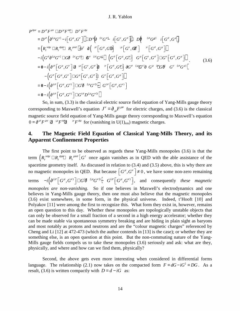
. (3.6)

So, in sum, (3.3) is the classical electric source field equation of Yang-Mills gauge theory

corresponding to Maxwell’s equation ;J Fν µνµ= ∂ for electric charges, and (3.6) is the classical

magnetic source field equation of Yang-Mills gauge theory corresponding to Maxwell’s equation ; ; ;0 F F Fσ µν µ νσ ν σµ= ∂ + ∂ + ∂ for (vanishing in U(1)em) magnetic charges.

4. The Magnetic Field Equation of Classical Yang-Mills Theory, and its Apparent Confinement Properties The first point to be observed as regards these Yang-Mills monopoles (3.6) is that the term ( )R R R Gνσµ σµν µνσ τ

τ τ τ+ + once again vanishes as in QED with the able assistance of the

spacetime geometry itself. As discussed in relation to (3.4) and (3.5) above, this is why there are no magnetic monopoles in QED. But because , 0G Gµ ν ≠ , we have some non-zero remaining

terms ( );( ) ( ;[ ]) ( ), ,i G G G G G G Gσ µ ν σ µ ν σ µ ν − ∂ + ∂ − , and consequently these magnetic

monopoles are non-vanishing. So if one believes in Maxwell’s electrodynamics and one believes in Yang-Mills gauge theory, then one must also believe that the magnetic monopoles (3.6) exist somewhere, in some form, in the physical universe. Indeed, t’Hooft [10] and Polyakov [11] were among the first to recognize this. What form they exist in, however, remains an open question to this day. Whether these monopoles are topologically unstable objects that can only be observed for a small fraction of a second in a high energy accelerator; whether they can be made stable via spontaneous symmetry breaking and are hiding in plain sight as baryons and most notably as protons and neutrons and are the “colour magnetic charges” referenced by Cheng and Li [12] at 472-473 (which the author contends in [13] is the case); or whether they are something else, is an open question at this point. But the non-commuting nature of the Yang-Mills gauge fields compels us to take these monopoles (3.6) seriously and ask: what are they, physically, and where and how can we find them, physically?

Second, the above gets even more interesting when considered in differential forms language. The relationship (2.1) now takes on the compacted form 2F dG iG DG= − = . As a result, (3.6) is written compactly with D d iG= − as:

J. R. Yablon

15

( ) ( ) ( ) ( )( ) ( )

2 2 2 3

2 3 2

P DF d iG F D dG iG d iG dG iG ddG idG iGdG G

i dG GdG G i dG GDG

= = − = − = − − = − − −

= − + − = − +0 0, (4.1)

where ( )R R R Gνσµ σµν µνσ τ

τ τ τ+ + is again responsible for 0dd = , “the exterior derivative of an

exterior derivative is zero.” So that term drops out as in Abelian gauge theory, but the remaining terms are non-vanishing. The correspondences between the non-zero terms in (3.6) and (4.1) are

2 ;( ),dG G Gσ µ ν ⇔ ∂ , ( ;[ ])GdG G Gσ µ ν⇔ ∂ , 3 ( ),G G G Gσ µ ν ⇔ and ( ;[ ])GDG G D Gσ µ ν⇔ . So

now, via (4.1) and the use of Gauss’/Stokes’ theorem dX X=∫∫ ∫� in differential forms, the

Yang-Mills magnetic monopole equation in integral form is:

( )( ) ( )( )( ) ( )

2 3 2 3

2 3 2 3

2 2

P DF F iGF ddG i dG GdG G i dG GdG G

dG i G iGdG G i G iGdG G

dG i G i GDG i G i GDG

= = − = − + − = − + −

= − − + = − − +

= − − = − −

∫∫∫ ∫∫∫ ∫∫ ∫∫∫ ∫∫∫ ∫∫∫

∫∫ ∫∫ ∫∫∫ ∫∫ ∫∫∫

∫∫ ∫∫ ∫∫∫ ∫∫ ∫∫∫

0

0

�

� � �

� � �

.(4.2)

Importantly, we are able to apply Gauss’/Stokes’ theorem to 2 ;( ),dG G Gσ µ ν ⇔ ∂ but not to

( ;[ ])GdG G Gσ µ ν⇔ ∂ or 3 ( ),G G G Gσ µ ν ⇔ or ( ;[ ])GDG G D Gσ µ ν⇔ . Note also that (4.2)

embeds 0dG =∫∫� , which in (3.5) for electrodynamics tells us that there is no net magnetic field

flux across any closed two-dimensional surface. Above, the magnetic charge equation (3.5) of Maxwell’s theory, 0P F= =∫∫∫ ∫∫� , now becomes 2P F i GF i G i GDG= − = − −∫∫∫ ∫∫ ∫∫∫ ∫∫ ∫∫∫� � .

Now, focusing on the correspondence 2 ;( ),dG G Gσ µ ν ⇔ ∂ , let us expand the above

differential forms and combine with 2 2dG G=∫∫∫ ∫∫� to formally write (wedge products 13! dx dx dxσ µ ν∧ ∧ are considered to have already been summed):

( )2 ;( )

; ; ;

2

,

, , ,

3 ,

i dG i G G dx dx dx

i G G G G G G dx dx dx

i G G dx dx i G

σ µ νσ µ ν

σ µ ν µ ν σ ν σ µσ µ ν

µ νµ ν

− = − ∂

= − ∂ + ∂ + ∂

= − = −

∫∫∫ ∫∫∫

∫∫∫

∫∫ ∫∫� �

. (4.3)

Then let us use this with (3.6) to expand some key terms in (4.2), and thereafter consolidate using ; ;D iGµ µ µ= ∂ − thus 3iGdG G iGDG− − = − and some summed index renaming as follows:

J. R. Yablon

16

( )( )( )

( )

; ; ;

;[ ] ;[ ] ;[ ]

, , ,

, , ,

3

P P dx dx dx

R R R G dx dx dx

i G G G G G G dx dx dx

i G G G G G G dx dx dx

G G G G G G G G G dx dx dx

σµνσ µ ν

νσµ σµν µνσ ττ τ τ σ µ ν

σ µ ν µ ν σ ν σ µσ µ ν

σ µ ν µ ν σ ν σ µσ µ ν

σ µ ν µ ν σ ν σ µσ µ ν

=

= + +

− ∂ + ∂ + ∂

− ∂ + ∂ + ∂

− + +

= −

∫∫∫ ∫∫∫

∫∫∫

∫∫∫

∫∫∫

∫∫∫0 ;[ ]

2 3 2

2 3 2

, 3i G G dx dx i G D G dx dx dx

dG i G i G G G dG i G i GDG

i G i G G G i G i GDG

µ ν σ µ νµ ν σ µ ν −

= − − ∂ − = − −

= − − ∂ − = − −

∫∫ ∫∫∫

∫∫ ∫∫ ∫∫∫ ∫∫∫ ∫∫ ∫∫ ∫∫∫

∫∫ ∫∫∫ ∫∫∫ ∫∫ ∫∫∫0 0

�

� � � �

� �

. (4.4)

So we see that inside the monopole volume, ( )R R R G dx dx dxνσµ σµν µνσ τ

τ τ τ σ µ ν+ +∫∫∫ describes the

coupling of individual the 2 1N − gauge fields iG τ of i iG Gτ τλ= to the spacetime geometry,

and that this coupling via 0R R Rνσµ σµν µνστ τ τ+ + = conspires to result in 0dG =∫∫� . Thus the

geometry couples to the gauge fields in a manner that prevents gauge fields from net flowing in and out across closed surfaces enclosing the monopole for exactly the same reasons that there are no magnetic monopoles at all in Abelian gauge theory. What also does not net flow across any closed surface, but is nonetheless clearly contained within the overall volume represented by the triple integral, is ( )3 ( ;[ ])GDG GdG iG G D G dx dx dxσ µ ν

σ µ ν= − =∫∫∫ ∫∫∫ ∫∫∫ , whatever this

represents. This expression simply is not integrable with dX X=∫∫ ∫� . But whatever 2 3 ,G G G dx dxµ ν

µ ν = ∫∫ ∫∫� � represents, does net flow across a closed two-dimensional surface.

We shall demonstrate in section 11 that this term represents a net flow of mesons through the closed surfaces.

Third, making (3.6) even more interesting, as detailed in section 1 of the author’s [13], if we perform a local transformation dGFFF −=′→ on the field strength F, which in expanded form is written as [ ]' ( )F F F G xµν µν µν ν µ→ = −∂ , then we find from (4.2) as a direct result of

0dG =∫∫� which in electrodynamics includes the Maxwell equation 0B dA→ →

⋅ =∫∫� and Faraday’s

law ( / )E d l B t dA→ → → →

⋅ = − ∂ ∂ ⋅∫ ∫∫� , see after (3.5), that:

( )P F F F dG F′= → = − =∫∫∫ ∫∫ ∫∫ ∫∫ ∫∫� � � � . (4.5)

This means that the net flow of the field strength 2 2F dG i G i G= − = −∫∫ ∫∫ ∫∫ ∫∫� � � � across a closed

two dimensional surface is invariant under the local gauge-like transformation ][' µνµνµνµν GFFF ∂−=→ , and that this invariance is caused by the equation 0dG =∫∫� which in

J. R. Yablon

17

Maxwell theory is responsible for Faraday’s law and the absence of magnetic monopoles. So in

Yang-Mills theory, 0dG =∫∫� is responsible for the symmetry principle expressed in (4.5).

Fourth, we see from (4.4) that 3 ( ),G G G G dx dx dxσ µ ν

σ µ ν = ∫∫∫ ∫∫∫ is one of the non-

integrable terms. This involves pure antisymmetric three-field cubic interactions G G Gσ µ ν∧ ∧ among the gauge fields. While we shall avoid the use of the term “glueball” to describe this because this term already has certain technical meanings for which its use here might cause confusion, certainly this term contained within the monopole volume is an amalgam of pure interaction gauge fields which nicely displays the non-linearity of Yang-Mills gauge theory.

Now, as much as the MIT Bag Model reviewed in, e.g., [14] section 18 has certain inelegant features such as the ad hoc introduction of backpressures to force confinement, this model very correctly makes one very important point that deserves utmost attention beyond the specifics of any particular model of confinement: focus carefully on what flows and does not flow across any closed two-dimensional surface. This is why the integral form of Maxwell’s equations is so vital to any sensible discussion of confinement. The confinement of gauge fields (which in strong SU(3)C are represented by the eight gluons of i iG Gτ τλ= with 1,2,3...8i = ) is

symbolically specified by Gluons 0=∫∫� . Similarly, the confinement of individual quarks (which

are represented by the SU(3)C Dirac wavefunction ; 1,2,3A Aψ = with three color eigenstates R,

G, B) is specified symbolically by Quarks 0=∫∫� . Different theories may have different ways to

achieve these two symbolic confinements, but in the end, one should pay close attention to the two-dimensional closed surface integrals and carefully examine what does and does not flow across these closed surfaces. Equations (4.2) through (4.5) contain a lot of information about what does and does not flow across the closed ∫∫� surface of a Yang-Mills monopole, so as

taught by the MIT Bag Model, we should study these equations carefully to see if these magnetic monopoles exhibit any attributes of confined gluons and quarks, or interactions via mesons.

A first point is made by ( )R R R G dx dx dxνσµ σµν µνσ ττ τ τ σ µ ν+ +∫∫∫ which leads to 0dG =∫∫�

in (4.4) and is the exact same expression which yields the absence of magnetic monopoles entirely, in Abelian electrodynamics, review (3.4). This ( )R R R G dx dx dxνσµ σµν µνσ τ

τ τ τ σ µ ν+ +∫∫∫

term contains an individual gauge field i iG Gτ τλ= , zeroed out from any net surface flow as a direct result of its coupling through the Riemannian geometry in the configuration of the first Bianchi identity, which upon Gauss’ / Stokes’ integration yields 0dG =∫∫� . So the question, in

the context of the MIT bag model, is whether this term is to be interpreted as telling us that gauge fields (gluons in SU(3) QCD) are confined, which means that there is never a net flow of gauge fields across any closed surface surrounding a Yang-Mills magnetic monopole. Recall that in electrodynamics, magnetic fields can and do flow, in net, through open surfaces, but because magnetic fields are aterminal fields, an outward flux over one portion of a closed surface is always cancelled by an inward flux across another portion of the closed surface. This interpretation of (4.4) as saying that there is no net flow of gauge fields across a closed Yang-

J. R. Yablon

18

Mills monopole surface is strengthened by the fact displayed in (4.5) that F F F′→ =∫∫ ∫∫ ∫∫� � �

is invariant under the local transformation dGFFF −=′→ , i.e., ][' µνµνµνµν GFFF ∂−=→ which renders the gauge fields Gµ (gluons in QCD) not observable with respect to net flux through the closed surface. This may mean as argued in section 1 of [13] that gauge fields are confined within the non-vanishing magnetic monopoles of Yang-Mills gauge theory for the exact same geometric reasons that magnetic monopoles do not exist at all in Abelian gauge theory. A second point is made by the term 2 2 3 ,dG G G G dx dxµ ν

µ ν = = ∫∫∫ ∫∫ ∫∫� � detailed in

(4.3). This is only non-vanishing integrable term in (4.4), as so tells us the crux of what does net flow across closed surfaces of a Yang-Mills magnetic monopole: the only thing that does net flow, are these 3 ,G Gµ ν entities. While we still must determine, physically, what these

3 ,G Gµ ν entities represent, we do know that , 0G Gµ ν ≠ is at the heart of the non-Abelian

character of Yang-Mills theories, see (2.1). If these 3 ,G Gµ ν do not turn out to represent

individual quarks, then because there are no other non-vanishing integrable terms in (4.4), what (4.4) would be telling us, in the sense of the MIT bag model, is that neither individual gluons nor individual quarks net flow across the closed surfaces of a Yang-Mills magnetic monopole, that is, that Gluons 0=∫∫� and Quarks 0=∫∫� . But what we also know is that baryons interact via

meson exchange, and that mesons have a color wavefunction of the form BBGGRR ++ . So mesons should be permitted to flow in and out of baryons, that is, we should also have

Mesons 0≠∫∫� . So if we can show that 2 3 ,G G G dx dxµ νµ ν = ∫∫ ∫∫� � represents meson flow, as

we shall do in section 11, then these magnetic monopoles, in the setting of spacetime geometry, would forbid net quark and gluon flows but permit net meson flow, and we would have some very strong formal reasons for identifying Yang-Mills magnetic monopoles with baryons.

A third point is made by the factors of “3” which also emerge in 2 3 ,G G G dx dxµ ν

µ ν = ∫∫ ∫∫� � and in ;[ ]3GDG G D G dx dx dxσ µ νσ µ ν=∫∫∫ ∫∫∫ in (4.3) and (4.4).

Although these arise from the three additive terms in the various expressions in (4.4), “3” also signifies the number of colors of quark in QCD, the number of quarks in a baryon, and the

number of terms in the meson color wavefunction BBGGRR ++ . So this “3” is a very strong hint – on top of the fact that Pσµν itself has three totally-antisymmetric spacetime indexes each capable of accommodating one of three vector current densities, and contains three additive terms – that there is some very definitive “three-ness” associated with these Yang-Mills monopoles. This “three-ness” could save us having to postulate that there are three quarks per baryon as is presently done in QCD, and could instead require us to have three quarks per baryon upon which we would then impose QCD as an Exclusion Principle. In other words, if this “three-ness” is telling us that a Yang-Mills monopole contains three quarks and has all the other required symmetries of a baryon including confinement and meson interaction, then postulating Yang-Mills theory would be synonymous with postulating QCD and postulating baryons and postulating that the baryons contain three colored quarks. This would make QCD itself an unavoidable, purely deductive consequence of Yang-Mills gauge theory, and would greatly strengthen the roots of QCD as a corollary theory to Yang-Mills gauge theory! It would at the

J. R. Yablon

19

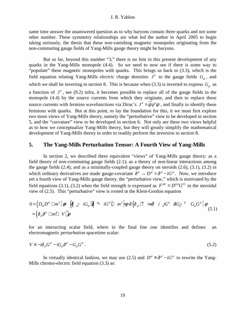
same time answer the unanswered question as to why baryons contain three quarks and not some other number. These symmetry relationships are what led the author in April 2005 to begin taking seriously, the thesis that these non-vanishing magnetic monopoles originating from the non-commuting gauge fields of Yang-Mills gauge theory might be baryons. But so far, beyond this number “3,” there is no hint in this present development of any quarks in the Yang-Mills monopole (4.4). So we need to now see if there is some way to “populate” these magnetic monopoles with quarks. This brings us back to (3.3), which is the field equation relating Yang-Mills electric charge densities Jν to the gauge fields Gµ , and

which we shall be inverting in section 8. This is because when (3.3) is inverted to express Gµ as

a function of Jν , see (9.2) infra, it becomes possible to replace all of the gauge fields in the monopole (4.4) by the source currents from which they originate, and then to replace these source currents with fermion wavefunctions via Dirac’s Jν νψγ ψ= , and finally to identify these fermions with quarks. But at this point, to lay the foundation for this, it we must first explore two more views of Yang-Mills theory, namely the “perturbative” view to be developed in section 5, and the “curvature” view to be developed in section 6. Not only are these two views helpful as to how we conceptualize Yang-Mills theory, but they will greatly simplify the mathematical development of Yang-Mills theory in order to readily perform the inversion in section 8. 5. The Yang-Mills Perturbation Tensor: A Fourth View of Yang-Mills In section 2, we described three equivalent “views” of Yang-Mills gauge theory: as a field theory of non-commuting gauge fields (2.1); as a theory of non-linear interactions among the gauge fields (2.4); and as a minimally-coupled gauge theory on steroids (2.6), (3.1), (3.2) in which ordinary derivatives are made gauge-covariant D iGµ µ µ µ∂ → = ∂ − . Now, we introduce yet a fourth view of Yang-Mills gauge theory, the “perturbative view,” which is motivated by the field equations (3.1), (3.2) when the field strength is expressed as ;[ ]F D Gµν µ ν= in the steroidal view of (2.5). This “perturbative” view is rooted in the Klein-Gordon equation

( ) ( )( )( ) ( )( )

2 2 2

2

0 D D m iG iG m m i G iG G G

m V

σ σ σ σ σ σ σσ σ σ σ σ σ σ

σσ

φ φ φ

φ

= + = ∂ − ∂ − + = ∂ ∂ + − ∂ − ∂ −

= ∂ ∂ + +(5.1)

for an interacting scalar field, where in the final line one identifies and defines an electromagnetic perturbation spacetime scalar: V i G iG G Gσ σ σ

σ σ σ≡ − ∂ − ∂ − . (5.2)

In virtually identical fashion, we may use (2.5) and D iGµ µ µ≡ ∂ − to rewrite the Yang-Mills chromo-electric field equation (3.3) as:

J. R. Yablon

20

( )( )( ) ( )( )( )( ) ( )( )

; ; 2 ; ; ; ;; ;

; 2 ; ;;

J g i G G G G m i G G G G G

g V m V G

ν µν σ σ σ σ µ ν µ ν µ ν µ νσ σ σ σ µ

µν σ µ ν µνσ µ

= ∂ ∂ − ∂ + ∂ − + − ∂ ∂ − ∂ + ∂ −

= ∂ ∂ + + − ∂ ∂ +,(5.3)

where in the final line, we have defined a “perturbation tensor” and its trace scalar:

( ); ;V i G G G Gµν µ ν µ ν µ ν≡ − ∂ + ∂ − , (5.4)

AB AB AB AC CBV V i G iG G G i G iG G Gσ σ σ σ σ σ σσ σ σ σ σ σ σ= = − ∂ − ∂ − = − ∂ − ∂ − . (5.5)

The perturbation scalar is identical in form to (5.2), but in Yang-Mills theory, it is an NxN Yang-Mills matrix of spacetime scalars, as we are reminded about by the explicit showing of Yang-Mills indexes in (5.5). Noting that for any two successive gauge-covariant derivatives:

( ) ( ); ; ; ; ; ; ; ; ;D D iG iG i G iG G G Vµ ν µ µ ν ν µ ν µ ν µ ν µ ν µ ν µν= ∂ − ∂ − = ∂ ∂ − ∂ − ∂ − = ∂ ∂ + , (5.6)

we see that in flat spacetime where ; ;, , 0µ ν µ ν ∂ ∂ = ∂ ∂ = , the antisymmetric combination:

[ ] ; ;, ,V V V D D D Dµν µν νµ µ ν µ ν = − = = . (5.7)

So the anti-symmetrized [ ]V µν is synonymous with the commutator of the Yang-Mills covariant derivatives. But in curved spacetime, using (5.7) to operate on a vector field Aσ and applying the Riemann curvature definition ; ;, G R Gσ

µ ν α αµν σ ∂ ∂ ≡ , we obtain:

[ ] [ ]( ); ; ; ;, ,D D A A V A R V Aµν µνµ ν σ µ ν σ σ σµν σ τ

τ τδ = ∂ ∂ + = + . (5.8)

Applying (5.8) and [ ]F D Gµν µ ν= to the magnetic monopole (3.6), the curvature terms

vanish as in (3.4) via 0R R Rνσµ σµν µνστ τ τ+ + = , and in both curved and flat spacetime, we obtain:

[ ] [ ] [ ] [ ]

; ;[ ] ; ;[ ] ; ;[ ]

; ; ; ; ; ;

( )

, , ,

P D D G D D G D D G

D D G D D G D D G

V G V G V G V G

σµν σ µ ν µ ν σ ν σ µ

σ µ ν µ ν σ ν σ µ

σµ µν νσ σµν σ µ ν

= + +

= + +

= + + =

. (5.9)

The Yang-Mills electric and magnetic field equations (3.1), (3.2) expressed in the respective wholly equivalent forms of (5.3) and (5.9), illustrate this fourth, “perturbative” view of Yang-Mills theory. In fact, it is a very useful exercise, to ask about the difference between the physics of Yang-Mills theory and that of ordinary Abelian gauge theory, which difference is wholly

J. R. Yablon

21

measured by the perturbation V µν of (5.4) and functions of this perturbation. It is this fourth view of Yang-Mills – the perturbative view – that will enable us to fill the “mass gap.”

To better understand the perturbative view, we introduce the labels “P” to denote “Perturbative,” “YM” to denote the complete, holistic (see [7] at page 356) physics encompassing all features of “Yang-Mills,” and “L” to denote the “Linear” expressions of Abelian gauge theories, most notably electrodynamics. Schematically, YM=L+P, that is, the complete physics of Yang-Mills YM theory may be thought of and analyzed as the sum of a perturbative aspect P and a linear aspect L. Thus, from (5.3), we can deduce that the perturbative-only portion of the current density, PJν , which is the difference YM LJ Jν ν− between

the complete Yang-Mills current density YMJν of (5.3) and the linear density

( )( ); 2 ; ;;LJ g m Gν µν σ µ νσ µ= ∂ ∂ + − ∂ ∂ of Abelian theory, is given by:

( ) ( )( ) ( )( )( )

; 2 ; ; ; 2 ; ;; ;P YM LJ J J g V m V G g m G

g V V G

ν ν ν µν σ µ ν µν µν σ µ νσ µ σ µ

µν µνµ

≡ − = ∂ ∂ + + − ∂ ∂ + − ∂ ∂ + − ∂ ∂

= −.(5.10)

In other words, ( )PJ g V V Gν µν µν

µ= − summarizes all of the effects which are added to the

current density LJν of Abelian theory by the non-linear perturbations of Yang-Mills theory.

For the magnetic monopoles, of course, P YMP Pσµν σµν≡ , because as we are reminded by

(3.4) the monopole densities of Abelian gauge theory are zero, 0LPσµν = . We know this of

course from (3.4), but we also see this by inspection from (5.9) in which the non-vanishing magnetic monopole arises completely from the index-cyclical application of the antisymmetrized

perturbation operator [ ]V µν to Yang-Mills gauge fields Gσ , i.e., from [ ]( )P V Gσµσµν ν= . If 0V µν → , clearly the monopole densities 0Pσµν → . Yang-Mills monopoles are thus entirely a

creature of perturbation, as they equivalently are creatures of non-Abelian gauge fields, of non-linear gauge interactions, and of gauge theory on steroids. Those of course, are the four views of Yang-Mills theory that we have articulated so far. Now we turn to a fifth view, which is the geometric curvature view first articulated by Herrmann Weyl in the wake of Einstein’s 1915 General Theory of Relativity [15] based on the curvature of spacetime. 6. Hermann Weyl’s Gauge Theory and Gravitational Curvature: A Fifth, Geometric View of Yang-Mills

Hermann Weyl in 1918 [16], [17] first conceived the idea that electrodynamics might be

unified with gravitation by analyzing a “twisting” of vectors under parallel transport to measure the geometric curvature of a gauge space. While Weyl first conceived of this as a local “gauge” symmetry, in 1929 [18] he corrected his original misconception into the modern view of a local “phase” symmetry. Notwithstanding, the original misnomer “gauge” is still used to name Weyl’s theory, perhaps as a reminder to posterity that even the most bedrock physical theories are sometimes properly-conceived in the abstract but misconceived in some details that need to

J. R. Yablon

22

be worked out over time. While gravitation operates via the curvature of a physical, non-compact configuration space 4ℜ first pioneered by Minkowski [19] based on Einstein’s 1905 development of Lorentz invariance into Special Relativity [20], Weyl’s theory operates along the circle of an abstract phase space using a non-observable the local phase ( )expi xθ for Abelian

theory and ( ) ( )exp exp i ii x i xθ λ θ= with 21,2,3... 1i N= − for an SU(N) Yang-Mills theory.

The relationship (5.8) already illustrates Weyl’s curvature idea very clearly. We see that

the anti-symmetrized [ ]V µνστδ plays a role in Yang-Mills theory very similar to that played by

the Riemann tensor R σµντ in gravitational theory: each is a “curvature” measuring the degree to

which the spacetime derivatives do or do not commute. In fact, lowering all of the indexes on in (5.8), we see that in going from an Abelian gauge theory in curved spacetime to a Yang-Mills theory in curved spacetime, we make the operator replacement [ ]R R g Vτσµν τσµν τσ µν→ + when

operating on any vector Aτ . That is:

( ); ; [ ],g D D A R g V Aτ ττσ µ ν τσµν τσ µν = + . (6.1)

(Note that the ability to apply ; ;A g Aτ

β σ στ β∂ = ∂ for raising and lowering indexes on a vector

A g Aτσ στ= operated on by ;β∂ relies on the metricity ; 0gµ νσ∂ = of the metric tensor gνσ , and

specifically, on the calculation ( ); ; ; ; ;A g A g A g A g Aτ τ τ τβ σ β στ β στ στ β στ β∂ = ∂ = ∂ + ∂ = ∂ . This will

be implicitly used in a number of the upcoming index manipulations.) So just as Rτσµν

represents curvature in spacetime, [ ]g Vτσ µν represents curvature in Weyl’s gauge / phase space.

We note the leading role of the anti-symmetrized perturbation [ ]V µν in this curvature connection

space. It is also worth noting the superposition of the symmetric metric tensor gτσ against the

antisymmetric τσ indexes in the first two positions of the Riemann tensor, which means that the resulting operator [ ]R g Vτσµν τσ µν+ is non-symmetric. But this is absorbed in the operation on Aτ

which sums out the τ index, so that both sides of (6.1) have balanced spacetime symmetries.

In fact, we can and should apply the same curvature analysis to the gauge-covariant derivative in curved spacetime, ; ;D iGµ µ µ= ∂ − , which we now write operating on Aν as:

; ;D A A iG A A A iG Aαµ ν µ ν µ ν µ ν µν α µ ν= ∂ − = ∂ − Γ − . (6.2)

With minor manipulation, and using ( )1

, , ,2 g g gα µν να µ αµ ν µν αΓ = + − , we can reframe this as:

( );g D A g ig G Aα ααν µ αν µ α µν αν µ= ∂ − Γ − . (6.3)

So here, the curvature view is highlighted by the fact that when going from Abelian to Yang-Mills gauge theory in curved spacetime, we make the operator replacement

J. R. Yablon

23

ig Gα µν α µν αν µΓ → Γ + when operating on the vector Aα . Because α µνΓ captures the effects of

parallel transport in curved spacetime, we see that ig Gαν µ represents Weyl’s parallel transport in

gauge (phase) space. As with (6.1), the combined operator ig Gα µν αν µΓ + is non-symmetric,

because α µνΓ is symmetric in ,µ ν while ig Gαν µ is symmetric in ,α ν . And as with (6.1), this is

absorbed in the operation on Aα which sums out the α index. In contrast, however, the curvature operator [ ]R g Vτσµν τσ µν+ in (6.1) is a tensor, but the parallel transport operator

ig Gα µν αν µΓ + in (6.3) is not because α µνΓ is not a tensor. Only the entire

g ig Gαν µ α µν αν µ∂ − Γ − is a tensor operator.

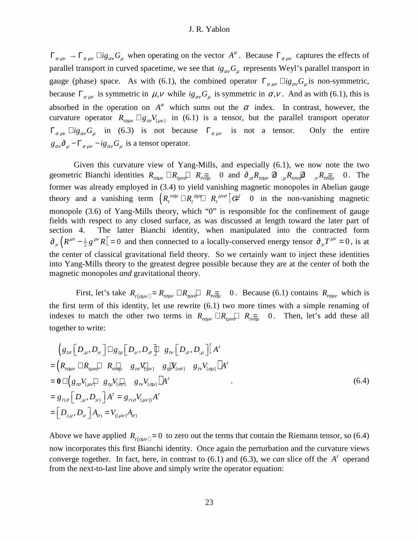
Given this curvature view of Yang-Mills, and especially (6.1), we now note the two

geometric Bianchi identities 0R R Rτσµν τµνσ τνσµ+ + = and ; ; ; 0R R Rα τσµν µ τσνα ν τσαµ∂ + ∂ + ∂ = . The

former was already employed in (3.4) to yield vanishing magnetic monopoles in Abelian gauge theory and a vanishing term ( ) 0R R R Gνσµ σµν µνσ τ

τ τ τ+ + = in the non-vanishing magnetic

monopole (3.6) of Yang-Mills theory, which “0” is responsible for the confinement of gauge fields with respect to any closed surface, as was discussed at length toward the later part of section 4. The latter Bianchi identity, when manipulated into the contracted form

( )1; 2 0R g Rµν µνν∂ − = and then connected to a locally-conserved energy tensor ; 0Tµν

ν∂ = , is at

the center of classical gravitational field theory. So we certainly want to inject these identities into Yang-Mills theory to the greatest degree possible because they are at the center of both the magnetic monopoles and gravitational theory.

First, let’s take ( ) 0R R R Rτσµν τµνσ τνσµτ σµν = + + = . Because (6.1) contains Rτσµν which is

the first term of this identity, let use rewrite (6.1) two more times with a simple renaming of indexes to match the other two terms in 0R R Rτσµν τµνσ τνσµ+ + = . Then, let’s add these all

together to write:

( )( )

( )

; ; ; ; ; ;

[ ] [ ] [ ]

[ ] [ ] [ ]

( ; ; ) ( [ ])

;( ; ) ([ ] )

, , ,

,

,

g D D g D D g D D A

R R R g V g V g V A

g V g V g V A

g D D A g V A

D D A V A

ττσ µ ν τµ ν σ τν σ µ

ττσµν τµνσ τνσµ τσ µν τµ νσ τν σµ

ττσ µν τµ νσ τν σµ

τ ττ σ µ ν τ σ µν

µ ν σ µν σ

+ +

= + + + + +

= + + +

= =

= =

0 . (6.4)

Above we have applied ( ) 0Rτ σµν = to zero out the terms that contain the Riemann tensor, so (6.4)

now incorporates this first Bianchi identity. Once again the perturbation and the curvature views converge together. In fact, here, in contrast to (6.1) and (6.3), we can slice off the Aτ operand from the next-to-last line above and simply write the operator equation:

J. R. Yablon

24

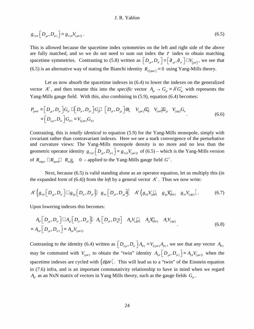
( ; ; ) ( [ ]),g D D g Vτ σ µ ν τ σ µν = . (6.5)

This is allowed because the spacetime index symmetries on the left and right side of the above are fully matched, and so we do not need to sum out index the τ index to obtain matching spacetime symmetries. Contrasting to (5.8) written as [ ]; ; ; ;, ,D D Vµ ν µ ν µν = ∂ ∂ + , we see that

(6.5) is an alternative way of stating the Bianchi identity ( ) 0Rτ σµν = using Yang-Mills theory.

Let us now absorb the spacetime indexes in (6.4) to lower the indexes on the generalized vector Aτ , and then rename this into the specific vector i iA G Gµ µ µλ→ = with represents the

Yang-Mills gauge field. With this, also combining in (5.9), equation (6.4) becomes:

; ; ; ; ; ; [ ] [ ] [ ]

;( ; ) ([ ] )

, , ,

,

P D D G D D G D D G V G V G V G

D D G V G

µνσ µ ν σ ν σ µ σ µ ν µν σ νσ µ σµ ν

µ ν σ µν σ

= + + = + +

= =

. (6.6)

Contrasting, this is totally identical to equation (5.9) for the Yang-Mills monopole, simply with covariant rather than contravariant indexes. Here we see a stark convergence of the perturbative and curvature views: The Yang-Mills monopole density is no more and no less than the

geometric operator identity ( ; ; ) ( [ ]),g D D g Vτ σ µ ν τ σ µν = of (6.5) – which is the Yang-Mills version

of 0R R Rτσµν τµνσ τνσµ+ + = – applied to the Yang-Mills gauge field Gτ .

Next, because (6.5) is valid standing alone as an operator equation, let us multiply this (in the expanded form of (6.4)) from the left by a general vector Aτ . Thus we now write:

( ) ( ); ; ; ; ; ; [ ] [ ] [ ], , ,A g D D g D D g D D A g V g V g Vτ ττσ µ ν τµ ν σ τν σ µ τσ µν τµ νσ τν σµ + + = + + . (6.7)

Upon lowering indexes this becomes:

; ; ; ; ; ; [ ] [ ] [ ]

( ; ; ) ( [ ])

, , ,

,

A D D A D D A D D A V A V A V

A D D A V

σ µ ν µ ν σ ν σ µ σ µν µ νσ ν σµ

σ µ ν σ µν

+ + = + +

= =

. (6.8)

Contrasting to the identity (6.4) written as ;( ; ) ([ ] ),D D A V Aµ ν σ µν σ = , we see that any vector )Aσ

may be commuted with [ ]V µν to obtain the “twin” identity ( ; ; ) ( [ ]),A D D A Vσ µ ν σ µν = when the

spacetime indexes are cycled with ( )σµν . This will lead us to a “twin” of the Einstein equation

in (7.6) infra, and is an important commutativity relationship to have in mind when we regard Aσ as an NxN matrix of vectors in Yang Mills theory, such as the gauge fields Gσ .

J. R. Yablon

25

Speaking of which, let us do just that. If we again set i iA G Gµ µ µλ→ = as we did for

(6.6), then (6.8) becomes ( ; ; ) ( [ ]),G D D G Vσ µ ν σ µν = , which is a “twin” of the magnetic monopole

equation (6.6) in which the gauge fields appear on the left rather than the right. But because the gauge fields are contained within ; ;D iGµ µ µ= ∂ − , let us set the vector ;A Dσ σ→ in both the

bottom line of (6.4) and in (6.8), and then use the Jacobian (determinant-related) identity

[ ] [ ] [ ], , , , , , 0a b c b c a c a b + + = to combine the twins (6.4) and (6.8) into the single

relationship:

;( ; ; ) ([ ] ; ) ;( ; ; ) ;( [ ]), ,D D D V D D D D D Vµ ν σ µν σ σ µ ν σ µν = = = . (6.9)

Because this commutes ;(D σ to the left of the commutator ; ; ),D Dµ ν in ;( ; ; ),D D Dσ µ ν , this

sets up the ability to now incorporate the remaining Bianchi identity

;( | | ) ; ; ; 0R R R Rα τσ µν α τσµν µ τσνα ν τσαµ∂ ≡ ∂ + ∂ + ∂ = which underpins the expression

( )1; 2 0R g Rµν µνν∂ − = that is at the heart of gravitational theory. In this second Bianchi identity

;( | | ) 0Rα τσ µν∂ = , we define the notation | |τσ as a “wall” to seal off the τσ indexes (this is not an

absolute value symbol as used here) from the ( )σµν cycling of the remaining free indexes. But

before we do this, let us work from the final expression in (6.6), use ;iD i Gσ σ σ= ∂ + inverted into

) ) ; )G iD iσ σ σ= − ∂ to replace )Gσ , and then the final line apply the Jacobian identity (6.9). The

result is:

( ) ( )( ) ( )( ) ( )

;( ; ) ([ ] ) ;( ; ) ; ) ([ ] ) ; )

;( ; ) ;( ; ; ) ([ ] ) ([ ] ; )

;( ; ; ) ;( ; ; ) ;( [ ]) ([ ] ; )

, ,

, ,

, ,

P D D G V G D D iD i V iD i

i D D D D D i V D V

i D D D D D i D V V

µνσ µ ν σ µν σ µ ν σ σ µν σ σ

µ ν σ µ ν σ µν σ µν σ

σ µ ν µ ν σ σ µν µν σ

= = = − ∂ = − ∂

= − ∂ = − ∂

= − ∂ = − ∂

. (6.10)

In this form, we have now turned the magnetic monopole density itself, entirely into an operator! Now, let’s move on to the second Bianchi identity ;( | | ) 0Rα τσ µν∂ = . We start with (6.1)

written in the form ; ; [ ],D D A R A V Aτµ ν σ τσµν µν σ = + . We operate on all three terms from the left

using ;Dα . Thus, ( ) ( ) ( ); ; ; ; ; [ ],D D D A D R A D V Aτα µ ν σ α τσµν α µν σ = + . Then we replicate this

expression two more times via a simple renaming of indexes with a cycling of , ,µ ν α . We then

add all of these together, and in the final line consolidate with the ( )αµν cyclator to fashion:

J. R. Yablon

26

( ) ( ) ( )( ) ( ) ( ) ( ) ( ) ( )( ) ( ) ( )

; ; ; ; ; ; ; ; ;

; ; ; ; [ ] ; [ ] ; [ ]

;( ; ; ) ;( | | ) ;( [ ])

, , ,

,

D D D A D D D A D D D A

D R A D R A D R A D V A D V A D V A

D D D A D R A D V A

α µ ν σ µ ν α σ ν α µ σ

τ τ τα τσµν µ τσνα ν τσαµ α µν σ µ να σ ν αµ σ

τα µ ν σ α τσ µν α µν σ

+ +

= + + + + +

= = +

. (6.11)

It should be clear how the term ( );( | | )D R Aτα τσ µν sets up the ability to apply and thereby embed

the second Bianchi identity ;( | | ) 0Rα τσ µν∂ = into Yang-Mills theory. So now let’s proceed.

We can slightly expand the compacted form in the bottom line of (6.11) using

;( ;( (D iGα α α= ∂ − , take the spacetime derivative ;(α∂ using the product rule, and make use of the

Bianchi identity ;( | | ) 0Rα τσ µν∂ = to write ( );( | | ) ( ; )R A R Aτ τα τσ µν τσ µν α∂ = + ∂0 , thus obtaining:

( ) ( ) ( ) ( )( ) ( )

( )

;( ; ; ) ;( | | ) ( | | ) ;( [ ])

;( | | ) ( ; ) ( | | ) ;( [ ])

( ; ) ( | | ) ;( [ ])

,D D D A R A iG R A D V A

R A R A iG R A D V A

R A iG R A D V A

τ τα µ ν σ α τσ µν α τσ µν α µν σ

τ τ τα τσ µν τσ µν α α τσ µν α µν σ

τ ττσ µν α α τσ µν α µν σ

= ∂ − +

= ∂ + ∂ − +

= + ∂ − +0

. (6.12)

That is it! We have now incorporated the Bianchi identity ;( | | ) 0Rα τσ µν∂ = which underlies the

geometric heart of gravitational theory, ( )1; 2 0R g Rµν µνν∂ − = , directly into Yang-Mills. Now

what remains is to rework (6.12) to make some of its meanings more transparent.

Continuing with (6.12), in the third line below we commute ;( | | ) ( ; )G R R Gα τσ µν τσ µν α= ,

because while Rτσµν is a spacetime fourth rank tensor, it is simply a 1x1 matrix in Yang-Mills

theory. In other words, while Gα and are ;Dα and [ ]V µν are all NxN matrices which do not

mutually commute with one another or even with themselves when the spacetime indexes are different, Rτσµν and (when it appears) gµν can be freely moved to any left-right position as

desired. In the fourth line we consolidate the first and second term using ; ) ; ) )D iGα α α= ∂ − . In

the fifth line we use ; ) ; ) )D iGα α α= ∂ − to expand the ( );( [ ])D V Aα µν σ term. In the sixth line we

apply the product rule for the ordinary derivative, and in the seventh line we reconsolidate the second and fourth terms using ;( ;( (D iGα α α= ∂ − . The result is:

J. R. Yablon

27

( ) ( ) ( ) ( )( )( )

( )( )

;( ; ; ) ;( | | ) ( | | ) ;( [ ])

( ; ) ( | | ) ;( [ ])

( ; ) ( ) ;( [ ])

( ; ) ;( [ ])

( ; ) ;( [ ]) ( [

,D D D A R A iG R A D V A

R A iG R A D V A

R A iR G A D V A

R D A D V A

R D A V A iG V

τ τα µ ν σ α τσ µν α τσ µν α µν σ

τ ττσ µν α α τσ µν α µν σ

τ ττσ µν α τσ µν α α µν σ

ττσ µν α α µν σ

ττσ µν α α µν σ α

= ∂ − +

= ∂ − +

= ∂ − +

= +

= + ∂ − ])

( ; ) ;( [ ]) ([ ] ; ) ( [ ])

( ; ) ;( [ ]) ([ ] ; )

A

R D A V A V A iG V A

R D A D V A V A

µν σ

ττσ µν α α µν σ µν α σ α µν σ

ττσ µν α α µν σ µν α σ

= + ∂ + ∂ −

= + + ∂

. (6.13)

Now the “odd duck” is the ([ ] ; )V Aµν α σ∂ which contains the only remaining ordinary

covariant derivative ; )α∂ amidst all the other ;(D α . But from (6.10) rearranged and right-

multiplied by Aσ :

([ ] ; ) ;( [ ])V A D V A iP Aµν α σ α µν σ µνα σ∂ = + , (6.14)

which is why we wanted to make the one final connection in (6.10) before turning to

;( | | ) 0Rα τσ µν∂ = . So we use (6.14) in (6.13) to finally write (6.13) in terms of Pµνα as:

( )( ; ) ;( ; ; ) ;( [ ]), 2P A iR D A iD D D A iD V Aτµνα σ τσ µν α α µ ν σ α µν σ = − + . (6.15)

This is our final result for the magnetic source density written as an operator operating on any vector Aσ , and it embeds both of the Bianchi identities as well as the Jacobian identity. We also

manipulate indexes (implicitly using ; 0gµ νσ∂ = ) to clearly display the spacetime symmetries:

( )( ; ) ;( ; ; ) ;( [ ]), 2g P A iR D A ig D D D A ig D V Aτ τ τ τστ µνα τσ µν α στ α µ ν στ α µν = − + . (6.16)

Of course, Aτ represents anything that transforms like a four-vector in spacetime. Among the specific vectors which may be of interest, are yet a fourth gauge covariant derivative

;A Dµ µ→ , and a gauge field A Gµ µ→ (which is implicit in ;A Dµ µ→ ). Thus, it helps to rewrite and reorder (6.15) with ;A Dµ µ→ to form:

( ) ;;( ; ; ) ; ( ; ) ; ;( [ ]) ;, 2D D D D R D D iP D D V Dτ

α µ ν σ τσ µν α µνα σ α µν σ = + + . (6.17)

In particular, this is now an operator identity which tells us what happens when we take four

successive gauge covariant derivatives in the ( );( ; ; ) ;,D D D Dα µ ν σ cyclic combination, as a

function of the Riemann curvature, the monopole density, and the perturbation!

J. R. Yablon

28

Finally, in flat spacetime, where 0Rτσµν = and ;D Dµ µ→ , (6.15) reduces in view of

(5.7), namely [ ] ,V D Dµν µ ν = , see also (6.10), simply to:

( ) ( )( )

( ) ( [ ]) ( ) ( )

( ) ( )

, 2 , 2 ,

, ,

P A iD D D A iD V A iD D D A iD D D A

i D D D D D A

µνα σ α µ ν σ α µν σ α µ ν σ α µ ν σ

α µ ν µ ν α σ

= − + = − +

= − ∂

. (6.18)

For A Dσ σ→ , contrast (6.10), this becomes:

( ) ( )( ) ( [ ]) ( ) ( )

( ) ( )

, 2 , 2 ,

, ,

P D iD D D D iD V D iD D D D iD D D D

iD D D D i D D D

µνα σ α µ ν σ α µν σ α µ ν σ α µ ν σ

α µ ν σ µ ν α σ

= − + = − +

= − ∂

.(6.19)

Alternatively and equivalently, explicitly showing a succession of four gauge-covariant derivatives in flat spacetime, the above becomes (contrast (6.17) for curved spacetime):

( )( ) ( ), ,D D D D D D iP Dα µ ν σ µ ν α µνα σ = ∂ − . (6.20)

So Hermann Weyl’s curvature view of Yang-Mills theory teaches us quite a bit, in

particular, about the nature of the Yang-Mills monopole densities. This ought not to be surprising, because the two Bianchi densities 0R R Rτσµν τµνσ τνσµ+ + = and

; ; ; 0R R Rα τσµν µ τσνα ν τσαµ∂ + ∂ + ∂ = contain cyclic index structures just as do the monopoles.

Above, we have illustrated the curvature analogy between gauge theory and gravitation, and embedded these two important identities of spacetime geometry in the Yang-Mills identity (6.15), i.e., (6.16). Based on this embedding, however, we can go even further, to fully unify classical Yang-Mills gauge theory with classical gravitation.

7. The Classical Gravitational Field Equation for Yang-Mills Gauge Theory, Inclusive of Maxwell’s Electrodynamics Because the second Bianchi identity ; ; ; 0R R Rα τσµν µ τσνα ν τσαµ∂ + ∂ + ∂ = is embedded in

(6.15) aka (6.16), there should be some manipulation that will reveal a Yang-Mills analog to the equation ( )1

; 2 0R g Rµν µνν∂ − = which underlies gravitational theory. We now deduce that.

We start by reconfiguring (6.16) according to the following sequence of steps which apply ;( ;( (D iGα α α= ∂ − and the product rule for differentiation. The bottom line consolidates the

second and fourth terms in the next-to-last line:

J. R. Yablon

29

( )( )

( ; ) ;( ; ; ) ;( [ ])

( ; ) ;( ; ; ) ( ; ; ) ;( [ ])

( ; ) ;( ; ; ) ;( ; ) ; )

, 2

, , 2

, ,

g P A iR D A ig D D D A ig D V A

iR D A ig D D A g G D D A ig D V A

iR D A ig D D A ig D D A

τ τ τ τστ µνα τσ µν α στ α µ ν στ α µν

τ τ τ ττσ µν α στ α µ ν στ α µ ν στ α µν

τ ττσ µν α στ α µ ν στ µ ν α

= − +

= − ∂ − +

= − ∂ − ∂ ( ; ; ) ;( [ ])

( ; ) ;( ; ; ) ;( ; ; ) ;( [ ])

, 2

, , 2

g G D D A ig D V A

iR D A ig D D D A ig D D A ig D V A

τ τ τστ α µ ν στ α µν

τ τ τ ττσ µν α στ α µ ν στ µ ν α στ α µν

− +

= − − ∂ +

.(7.1)

Now, because Aτ is just a dummy operand which can be any four-vector, let us just lop it off of (7.1) entirely. The equations on each side of the equal sign will no longer have matching symmetries because gστ is symmetric while Rτσµν is antisymmetric in these same two indexes.

So we shall use a “=” sign, that is, an equal sign in quotes to designate the equality of the left and right sides of (7.1) when operating on Aτ which acquires a mismatched symmetry when the operand Aτ is removed. Thus, we now write:

( ; ) ;( ; ; ) ;( ; ; ) ;( [ ])" " , , 2g P iR D ig D D D ig D D ig D Vστ µνα τσ µν α στ α µ ν στ µ ν α στ α µν = − − ∂ + . (7.2)

The two sides of this equation are only equal when they operate on a vector Aτ as in (7.1), or if the symmetries can be restored in some other way. So we will need to now manipulate this such that the symmetries on both sides once again become matching and the equality is restored. First, we fully expand the cyclators in (7.2) to obtain:

; ; ;

; ; ; ; ; ; ; ; ;

; ; ; ; ; ; ; ; ;

; [ ] ; [ ] ; [ ]

" "

, , ,

, , ,

2 2 2

g P iR D iR D iR D

ig D D D ig D D D ig D D D

ig D D ig D D ig D D

ig D V ig D V ig D V

στ µνα τσµν α τσνα µ τσαµ ν

στ α µ ν στ µ ν α στ ν α µ

στ µ ν α στ ν α µ στ α µ ν

στ α µν στ µ να στ ν αµ

= + +

− − −

− ∂ − ∂ − ∂

+ + +

. (7.3)

Next, we use the terms ;R Dτσµν α and the like as a guide and engage in the same manipulations

normally used to derive ( )1; 2 0R g Rµν µνν∂ − = from ; ; ; 0R R Rα τσµν µ τσνα ν τσαµ∂ + ∂ + ∂ = . We raise

τσ indexes everywhere to put the Riemann tensor into mixed form so we can extract the Ricci tensor. Then we contract one pair of indexes by setting ν τ= and we start to reveal the Ricci tensor via R Rτσ σ

µτ µ= including revealing one sign reversal via R Rτσ στα α= − . This yields the

intermediate result:

; ; ;

; ; ; ; ; ; ; ; ;

; ; ; ; ; ; ; ; ;

; [ ] ; [ ] ; [ ]

" "

, , ,

, , ,

2 2 2

g P iR D iR D iR D

ig D D D ig D D D ig D D D

ig D D ig D D ig D D

ig D V ig D V ig D V

στ σ σ τσµτα µ α α µ αµ τ

στ στ στα µ τ µ τ α τ α µ

στ στ στµ τ α τ α µ α µ τ

στ στ στα µτ µ τα τ αµ

= − +

− − −

− ∂ − ∂ − ∂

+ + +

. (7.4)

J. R. Yablon

30

Now we do a second index contraction by setting µ σ= . This yields the Ricci scalar R Rσσ =

and allows another application of R Rτσ τασ α= − with a second sign reversal. We then use the gτσ

to raise indexes. Now we have:

; ; ;

; ; ;; ; ; ; ; ;

; ; ;; ; ; ; ; ;

[ ; ]; ] [ ] ; [

, , ,

, , ,

2 2 2

P iRD iR D iR D

iD D D iD D D iD D D

i D D i D D i D D

iD V iD V iD V

τ σ ττα α α σ α τ

τ τ τα τ τ α τ α

τ τ ττ α τ α α τ

τ τ τα τ τα τ α

= − −

− − −

− ∂ − ∂ − ∂

+ + +

. (7.5)

Above, we have now removed the quotes from the equal sign, because now the only free

index is α and there is no longer a mismatched symmetry. That is, the symmetry became mismatched when we looped off Aτ from (7.1) and it became restored when we contracted down to (7.5) which is a vector equation containing one free index α . But given the commutation properties in the above, 0Pτ

τα = because it is a third-rank totally antisymmetric tensor, and all

of the other terms in the second, third and fourth lines also cancel out by inspection because of the various antisymmetries. So all that we have left in (7.5) after some very simple rearrangement, and applying the Einstein equation 1

2T R g Rµν µν µνκ− = − , is:

( )1; ;2 0T D R g R Dµν µν µνν νκ− = − = . (7.6)

This is the gravitational field equation of Yang-Mills theory! It resembles the usual

( )1; ; 2 0T R g Rµν µν µνν νκ− ∂ = ∂ − = , but here, we have an operator equation, the derivative is

moved to the right (it does not operate to differentiate 12R g Rµν µν− and so is a free derivative),

and it is a gauge-covariant derivative. This is a “twin” of the Einstein equation. If we want to highlight the nexus to Yang-Mills theory in the clearest way possible, we may expand the above into the form:

( ) ( )( )1; ;2 0T iG R g R iGµν µν µνν ν ν νκ− ∂ − = − ∂ − = . (7.7)

The latter expression ( )( )1

;2 0R g R iGµν µνν ν− ∂ − = fully marries Einstein’s curvature view of

spacetime with Weyl’s curvature view of gauge theory, and is a geometric identity of Yang-Mills (and even Abelian) gauge theory arising from incorporating both Bianchi identities ( ) 0Rτ σµν =

and ;( | | ) 0Rα τσ µν∂ = and the Jacobian [ ] [ ] [ ], , , , , , 0a b c b c a c a b + + = into the development

of section 6 to arrive at (6.15). And, if we then use this to operate on some arbitrary vector Aσ ,

we may further expand this to:

J. R. Yablon

31

( ) ( )( )( ) ( )( )( ) ( )( )( ) ( )( )

1; ;2

12

12

12

0 T A iG A R g R A iG A

T A A iG A R g R A A iG A

T i G A R g R A A iG A

T g ig G A R g R g ig G A

µν µν µνν σ ν σ ν σ ν σ

µν τ µν µν τν σ νσ τ ν σ ν σ νσ τ ν σ

µν τ τ τ µν µν τσ ν νσ σ ν τ ν σ νσ τ ν σ

µν τ µν µν ττσ ν τ νσ τσ ν τσ ν τ νσ τσ ν

κ

κ

κ δ δ

κ

= − ∂ − = − ∂ −

= − ∂ − Γ − = − ∂ − Γ −

= − ∂ − Γ − = − ∂ − Γ −

= − ∂ − Γ − = − ∂ − Γ −

. (7.8)

By the connection 1

2T R g Rµν µν µνκ− = − to T µν (sans cosmological constant, which one can

also inject into the development if desired), we further come to understand the coupling between gauge fields and source matter.

This brings Hermann Weyl full circle back to Albert Einstein, as there is no more concise

way to express the role of geometry in spacetime and in gauge space than through the “Einstein-Weyl” unified field equation ( )1

;2 0R g R Dµν µνν− = . The term 1

2R g Rµν µν− emerges from

Einstein’s understanding of parallel transport and curvature in spacetime, while ;D iGν ν ν= ∂ −

emerges from Weyl’s understanding of parallel transport and curvature in gauge (phase) space. The contracted combination of ( )1

;2 0R g R Dµν µνν− = marries the two together into one!

While we have developed the foregoing based on Yang-Mills gauge theory and generally

regarded ; ; ;i iD iG i Gν ν ν ν νλ= ∂ − = ∂ − to be an NxN matrix, this is not an absolute requirement.

Weyl developed ;D iGν ν ν= ∂ − twenty five years before Yang and Mills came on the scene. So

we can also take the gauge group to be U(1)em of electrodynamics, and we may regard the gauge field Gν as Maxwell’s electrodynamic vector potential Aν (here we are not taking Aν to be

arbitrary but making a specific association with the electromagnetic potential). When we do so, the geometric operator equation ( )( )1

;2 0R g R iAµν µνν ν− ∂ − = now becomes the classical unified

field equation for gravitation and electromagnetism. And because ( )( )1;2 0R g R iGµν µνν ν− ∂ − =

can be applied to SU(2)W and SU(3)C, we now have a complete classical unification of the field equations for all four known interactions: electromagnetic, weak, strong and gravitational! All of classical field theory is geometry! While recognizing the challenges of tractable calculation, unified quantum field theory then emerges, in principle, from the functional path integration

4exp expZ D i d x D iSφ φ= =∫ ∫ ∫L of the action 4S d x= ∫L for with the classical field equation

( )( )1;2 0R g R iGµν µνν ν− ∂ − = over all possible configurations Dφ of the classical fields

,g Gµµνφ = .

8. The Configuration Space Inverse of the Electric Charge Field Equation of Classical Yang-Mills Theory Much of the focus in the last two sections was centered on the classical Yang-Mills magnetic charge density Pσµν , primarily because this has the same index-cyclic, antisymmetric

J. R. Yablon

32

tensor properties as the two Bianchi identities 0R R Rτσµν τµνσ τνσµ+ + = and

; ; ; 0R R Rα τσµν µ τσνα ν τσαµ∂ + ∂ + ∂ = which along with the Jacobian identity

[ ] [ ] [ ], , , , , , 0a b c b c a c a b + + = which were central to the development of the classical

unified field equation in the various formulations of (7.6) to (7.8). Now it is time to return our focus largely to the field equation (3.3) of the classical Yang-Mills electric charge density Jν .

If we compare ( )( ); 2 ; ;;J g D D m D D Gν µν σ µ νσ µ= + − which is the electric charge density

field equation (3.3) side by side with ( );( ) ( ;[ ]),P i G G G D Gσµν σ µ ν σ µ ν = − ∂ + which is the

magnetic charge density field equation (3.6) while keeping in mind that the gauge-covariant derivative ; ;D iGµ µ µ= ∂ − , then we notice a remarkable thing: Mathematically, these two non-Abelian Maxwell’s equations can be thought of as a pair of parametric equations in which the gauge field Gµ is itself the parameter. These means in turn that there is a precise, definitive, albeit complicated relationship between the monopole density Pσµν and the charge density Jν . As such, we should endeavor to find out more about this relationship. Keep in mind, this would never become a consideration in Abelian electrodynamics, because there, the magnetic sources

0Pσµν = . But this is not the case in Yang-Mills theory.

Additionally, the magnetic density ( );( ) ( ;[ ]),P i G G G D Gσµν σ µ ν σ µ ν = − ∂ + of (3.6) aka

(4.1) looks on the surface like a bundle of gluons Gµ . (Again, we avoid the term “glueball” to avert confusion with specific meanings that have already been given to this term.) But if we take a conservative view of field theory, wherein gauge fields always originate from some source, then the natural progression from (3.6), (4.1) should be to inquire about the sources from which these gauge fields Gµ originate. Other than the monopole source Pσµν , the only other logical source of Gµ is the electric source density Jν . Furthermore, in Dirac theory, an electric source density Jν may in turn be expressed in

terms of fermion wavefunctions ψ . Specifically, Dirac’s equation says that ( ) 0i mµµγ ψ∂ − = .

For the adjoint spinor † 0ψ ψ γ= the field equation is 0i mµµψγ ψ∂ + = . Adding yields

( ) 0µµ ψγ ψ∂ = as is well known. And because the conserved current is expressed by 0J µ

µ∂ = ,

we identify the current density with J µ µψγ ψ= . In Yang-Mills theory, for a compact, simple

gauge group SU(N), this generalizes to i i i iCAB AB CD DJ Jµ µ µ µλ λ λ γ γ= = Ψ Ψ = Ψ Ψ , with Yang-

Mills adjoint i and fundamental A,B,C,D indexes explicitly shown for illustration, and where

AΨ = Ψ is an N-component column vector of 4-component elementary Dirac fermion

wavefunctions ψ . Thus, ( )( ); 2 ; ;;g D D m D D Gν µν σ µ νσ µγΨ Ψ = + − becomes another way to

write (3.3). With this progression from J µ µγ→ Ψ Ψ , the gauge field Gµ now is the parameter

which specifies a relationship between the magnetic sources Pσµν and the Dirac fermions Ψ . Because we already seen based on some of the symmetries outlined in section 4 that these Pσµν

J. R. Yablon

33

have attributes reminiscent of baryons, this parameterization may provide a way to “populate” these magnetic monopoles Pσµν with fermion eigenstates ψ . If, in turn, these fermion eigenstates exhibit the same symmetries as the quarks which we know reside inside baryons, this would provide support for regarding these ψ as quark wavefunctions, and the Pσµν themselves as baryon densities. So, we shall now proceed along these lines to populate the monopoles with

fermions by developing the inverse field equations G I J Iτ τµ τµ τµ γ≡ = Ψ Ψ .

Specifically, we now define an inverse Iτµ such that G I Jτµ τµ≡ . Then, we can insert

G I J Iτ τµ τµ τµ γ= = Ψ Ψ into ( );( ) ( ;[ ]),P i G G G D Gσµν σ µ ν σ µ ν = − ∂ + for each occurrence of the

gauge field Gµ , thereby populating Pσµν with fermions. As we shall now do, it helps to review how this inversion is done in electrodynamics, to prepare for the more complicated calculation required for Yang-Mills theory.

In U(1)em electrodynamics, we use the classical field equation mentioned between (3.3)

and (3.4) to specify this inverse LG I Jτµ τµ≡ , namely:

( )( ) ( )( ); 2 ; ; ; 2 ; ;; ; LJ g m G J g m I Jν µν σ µ ν ν τ µν σ µ ν τσ µ τ σ τµδ= ∂ ∂ + − ∂ ∂ = ≡ ∂ ∂ + − ∂ ∂ . (8.1)

We have specifically denoted this inverse LI τµ with a “L” subscript to keep note of the fact that

this is the linear inverse of Abelian gauge theory. We will shortly derive a more complicated inverse YMI τµ which includes all the effects of Yang-Mills theory both linear and non-linear, and

then from this will form a P YM LI I Iτµ τµ τµ≡ − which tells us the precise portion of the complete

Yang-Mills inverse YMI τµ arising from the perturbative effects which account for the difference

between YMI τµ and LI τµ . This follows the approach introduced prior to (5.10) where we found

that the perturbative-only contribution to the current density is ( )PJ g V V Gν µν µνµ= − . So now,

we are effectively seeking the inverse of this.

Dropping Jτ from the last two terms above with index renaming allows us to sift out:

( )( ); 2 ; ;; Lg m Iµ µτ σ τ µ

ν σ ντδ ≡ ∂ ∂ + − ∂ ∂ . (8.2)

Looking at the configuration space operator ( ); 2 ; ;

;g mµτ σ τ µσ∂ ∂ + − ∂ ∂ , we see that in flat

spacetime this is symmetric in its ,µ τ indexes, but in curved spacetime it is not. In curved

spacetime, the Riemann tensor ; ;, G R Gσµ ν α αµν σ ∂ ∂ ≡ is non-zero as noted just prior to (3.4),

and so left-right ordering matters. Especially since the non-Abelian ( ); 2 ; ;;g D D m D Dµτ σ µ τσ + −

in (3.3) with ; ;D iGµ µ µ= ∂ − where i iABG Gµ µλ= is an NxN matrix for SU(N) is manifestly not

,µ τ symmetric even in flat spacetime because of [ ] ,V D Dµν µ ν = in (5.7), it will be important

J. R. Yablon

34

to pay attention right away to commutativity issues. One will also discern from this, that except in flat spacetime for Abelian gauge theory, the inverse Iντ will be non-symmetric between its

,ν τ indexes. Thus, the definitional choice G I Jτν τν≡ where the left index in the inverse is

summed with the current density is different than the reversed-index definition G I Jτν ντ≡ in

which the right index is so-summed. Based on the terms in (8.2), we may surmise that ; ;LI g A Bντ ντ ν τ≡ + ∂ ∂ will be the general

form of the inverse, with LI ντ defined to have the same index ordering as ; ;ν τ∂ ∂ , and with A and

B being unknowns we shall now deduce. We define A and B to the right, so that when we insert

LI ντ into (8.2) to specify:

( )( )( ); 2 ; ;; ; ;g m g A Bµ µτ σ τ µ

ν σ ντ ν τδ ≡ ∂ ∂ + − ∂ ∂ + ∂ ∂ , (8.3)

the A and B will not come between the known terms. Again, this is part of our desire to pay very close attention to commutativity order right at the outset, because this will be especially important when we progress to Yang-Mills theory. Now we expand (8.3) to obtain:

( ) ( )( ); 2 ; ; 2 ; ; ;; ; ; ; ; ;m A A m Bµ µ σ µ σ µ τ µ

ν ν σ ν σ ν ν τδ δ= ∂ ∂ + − ∂ ∂ + ∂ ∂ + ∂ ∂ − ∂ ∂ ∂ ∂ , (8.4)

where we may freely commute gµν , and where we then make use of g gµ µτ

ν ντδ = and also use

the remaining metric tensors to raise or lower indexes as appropriate. The first step is to eliminate the ( ); 2

; m Aµ σν σδ ∂ ∂ + term by setting ( ); 2

; 1m Aσσ∂ ∂ + = , and more precisely, by left-

multiplying with ( ) 1; 2; mσσ

−∂ ∂ + to write:

( ) ( ) ( )1 1; 2 ; 2 ; 2; ; ;A m m A mσ σ σσ σ σ

− −= ∂ ∂ + ∂ ∂ + = ∂ ∂ + , (8.5)

Because ; 2; mσσ∂ ∂ + is not a matrix (shortly, its Yang-Mills counterpart will be), the use of

inverses is not required and we can employ the more-common ( ); 2;1/A mσσ= ∂ ∂ + . But this

“overkill” will be important for Yang-Mills theory. Inserting (8.5) back into (8.4) while maintaining all the “overkill” of ordering and taking inverses yields, with some rearrangement:

( ) ( )( )1; ; ; 2 ; 2 ; ; ; ; ;; ; ;m m Bν µ σ σ ν µ µ ν τσ σ τ

−∂ ∂ ∂ ∂ + = ∂ ∂ + ∂ ∂ − ∂ ∂ ∂ ∂ . (8.6)

Multiplying from the left by ( )( ) 1; 2 ; ; ; ; ;

; ;mσ ν µ µ ν τσ τ

−∂ ∂ + ∂ ∂ − ∂ ∂ ∂ ∂ then yields:

( )( ) ( )1 1; 2 ; ; ; ; ; ; ; ; 2; ; ;B m mσ ν µ µ ν τ ν µ σσ τ σ

− −= ∂ ∂ + ∂ ∂ − ∂ ∂ ∂ ∂ ∂ ∂ ∂ ∂ + . (8.7)

J. R. Yablon

35

Now using (8.5) and (8.7) in ; ;LI g A Bντ ντ ν τ≡ + ∂ ∂ we obtain:

( )( ) ( )1 1; 2 ; ; ; ; ; ; ; ; 2; ; ; ; ;I g m mσ α β β α σ α β σ

ντ ντ ν τ σ σ σ

− − = + ∂ ∂ ∂ ∂ + ∂ ∂ − ∂ ∂ ∂ ∂ ∂ ∂ ∂ ∂ +

. (8.8)

Since these inverses have a Yang-Mills dimension of NxN=1x1, they are not Yang-Mills matrices and may be placed into denominators in customary manner. Thus (8.8) becomes:

( ); ;

; ;

; 2 ; ; ; ; ;; ;

; 2;

L

gm

Im

α βν τ

ντ σ α β β α σσ σ

ντ σσ

∂ ∂ ∂ ∂+

∂ ∂ + ∂ ∂ − ∂ ∂ ∂ ∂=

∂ ∂ + . (8.9)

In flat spacetime where the derivatives may be freely commuted, we can factor out the ; ;α β∂ ∂ terms to leave a ; ;

; ; 0σ σσ σ∂ ∂ − ∂ ∂ = which also zeros out. Then, we convert to momentum space

via i kµ µ∂ → and add the iε+ prescription to yield the inverse for a massive vector boson::

2 2 2

2 2 2

i

L

k k k kg g g

m m mIm k k m k k m i

ν τ ν τ ν τεντ ντ ντ

ντ σ σ σσ σ σ ε

+∂ ∂+ − + − +

= = ⇒∂ ∂ + − − +

. (8.10)

We make note of the fact that up to a factor of i, this inverse is identical to the QED propagator

ντπ , i.e., that LiIντ ντπ = . Finally, we return to use the above in LG I Jτν τν≡ (note reversed index

ordering versus (8.10) traceable to (8.2)), which yields:

02

2 2

1 1m

k kg

mG J J Jk k m i k k m i k k i

τ ντν

τν ν νσ σ σ

σ σ σε ε ε=− +

= = − ⇒−− + − + +

. (8.11)

After a final flat spacetime commutation [ ] [ ], , 0k kν τ ν τ∂ ∂ = − = , the final reduction occurs via

conservation of charge density 0Jττ∂ = , which in momentum space, is 0k Jτ

τ = (e.g., [7] after

I.5(4)). Now, it is easy to see from (8.10) as 0m→ , via 2/k k mν τ → ∞ , that LI ντ → ∞ . This is

why the configuration space operator ; ; ;;gµν σ µ νσ∂ ∂ − ∂ ∂ for a massless vector particle in flat

spacetime has no inverse (e.g., [7] section 3.4). But what happens in curved spacetime when we use iε+ , and set 0m→ ? This will be instructive for our momentary consideration of Yang-Mills. In this circumstance, using (8.9) in LG I Jτ

ν τν= , the inverse equation corresponding to

(8.11), becomes:

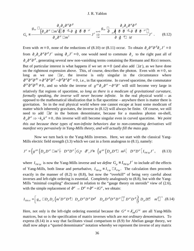
J. R. Yablon

36

( ) ( ); ; ; ;

; ; ; ;

; 2 ; ; ; ; ; ; ; ; ; ; ;0; ; ;

; 2 ;; ;

m

i

g gm

G J Jm i

α β α βτ ν τ ν

τν τνσ α β β α σ σ α β β α σσ σ στ τ

ν σ σεσ σ ε

=

+

∂ ∂ ∂ ∂ ∂ ∂ ∂ ∂+ +

∂ ∂ + ∂ ∂ − ∂ ∂ ∂ ∂ ∂ ∂ ∂ ∂ − ∂ ∂ ∂≡ ⇒

∂ ∂ + ∂ ∂ + . (8.12)

Even with 0m= , none of the reductions of (8.10) or (8.11) occur. To obtain ; ;

; ; 0Jα β τν τ∂ ∂ ∂ ∂ =

from ; ;; ; Jα β ττ ν∂ ∂ ∂ ∂ using ; 0Jτ

τ∂ = , one would need to commute ;τ∂ to the right past all of ; ;

;α β

ν∂ ∂ ∂ , generating several new non-vanishing terms containing the Riemann and Ricci tensors.

But of particular interest is what happens if we set 0m= (and also add iε+ ), as we have done on the rightmost expression above. This, of course, describes the photon. Even with 0m= , so long as we use iε+ , the inverse is only singular in the circumstance where

;[ ; ; ] ; ; ; ; ; ; 0σ α β σ α β β α σ∂ ∂ ∂ = ∂ ∂ ∂ − ∂ ∂ ∂ = , i.e., in flat spacetime. In curved spacetime, the commutator ;[ ; ; ] 0σ α β∂ ∂ ∂ ≠ , and so while the inverse of ; ; ;

;gµν σ µ νσ∂ ∂ − ∂ ∂ will still become very large in

relatively flat regions of spacetime, so long as there is a modicum of gravitational curvature, formally speaking, the inverse will never become infinite. In the real physical world – as opposed to the mathematical idealization that is flat spacetime – anywhere there is matter there is gravitation. So in the real physical world where one cannot escape at least some modicum of matter which inherently gravitates, the inverse in (8.12) will always be finite. Of course, we still need to add iε+ in the bottom denominator, because for a massless photon on-shell,

;; 0k kσ σσ σ∂ ∂ ⇒ − = , this inverse will still become singular even in curved spacetime. We point

this out because these types of non-infinite behaviors due to non-commuting derivatives will manifest very pervasively in Yang-Mills theory, and will actually fill the mass gap. Now we turn back to the Yang-Mills inverses. Here, we start with the classical Yang-Mills electric field strength (3.3) which we cast in a form analogous to (8.1), namely:

( )( ) ( )( ); 2 ; ; ; 2 ; ;; ; YMJ g D D m D D G J g D D m D D I Jν µν σ µ ν ν τ µν σ µ ν τσ µ τ σ τµδ= + − = ≡ + − , (8.13)

where YMI τµ is now the Yang-Mills inverse and we define YMG I Jτµ τµ≡ to include all the effects

of Yang-Mills, both linear and perturbative, YM L PI I Iτµ τµ τµ≡ + . The calculation then proceeds

exactly in the manner of (8.2) to (8.8), but now the “overkill” of being very careful about inverses and left-right ordering is essential. Completely analogously to (8.8), but with the Yang-Mills “minimal coupling” discussed in relation to the “gauge theory on steroids” view of (2.6), with the simple replacement of D iGµ µ µ µ∂ → = ∂ − , we obtain:

( ) ( )1 12 ; ; ; ; ; ; ; ; ; ; ; 2; ; ; ; ;YMI g D D m D D D D D D D D D D D D D D mα β σ α β β α σ α β σ

ντ ντ ν τ σ σ σ− − = + + − +

.(8.14)

Here, not only is the left-right ordering essential because the i i

ABG Gµ µλ= are all Yang-Mills

matrices, but so is the specification of matrix inverses which are not ordinary denominators. To express (8.14) in a way that facilitates visual comparison to (8.9) for Abelian gauge theory, we shall now adopt a “quoted denominator” notation whereby we represent the inverse of any matrix

J. R. Yablon

37

M according to 11/ " "M M −≡ . And to keep track of the proper placement of an inverse in the overall series of matrix multiplications, we use a “ ∨ ” down-arrow as a placement marker. In this notation, (8.14) now is written as:

; ;; ;

2 ; ; ; ; ; ; ; ;; ;

; 2;

" "

" "YM

D D D Dg

m D D D D D D D D D DI

D D m

α βν τ

ντ α β σ α β β α σσ σ

ντ σσ

∨

∨+

+ −=

+ . (8.15)

By comparison to (8.9), we see in stark relief the manner in which classical Yang-Mills gauge theory is simply Gauge theory on steroids with the minimal coupling principle

D iGµ µ µ µ∂ → = ∂ − . One should note two factorizations which are available in the upper

denominator of (8.15). The first two terms may be written as ( )2 ; ; ;;m D D D Dσ α βσ+ which

matches up with the ; ;D Dα β in the top numerator. But these do not simply factor out as they did going from (8.9) to (8.10) because of the Yang-Mills matrices and the inverses involved. And the latter two terms in the upper denominator may be written as ( ); ; ; ; ; ;

;D D D D D D Dσ α β β α σσ − .

As discussed after (8.12), this helps avert a singular numerator even if we set 0m= , because this will remain finite to the degree that ; ; ; ; ; ; ;[ ; ; ] 0D D D D D D D D Dσ α β β α σ σ α β− = ≠ . In section 10, this elimination of the Proca mass, 0m→ , will be of particular interest for filling the mass gap.

We note finally, referring back to sections 6 and 7, that the symmetries of sequences of covariant derivatives is integrally connected to the “curvature view” of Yang-Mills theory and helped us to derive the Einstein-Weyl equation (7.6). Along the way, beginning with (6.9), we obtained several useful identities involving the commutativity properties of taking three or four successive covariant derivatives. Clearly, based on these identities, as a general rule,

;[ ; ; ] 0D D Dσ α β ≠ . Thus, (8.15) will not become infinite even if we set 0m= and even if we do not include iε+ and even if the gauge particles for which (8.15) is the inverse are placed on shell without iε+ . These properties of (8.15) will become essential for filling the mass gap. 9. Populating Yang-Mills Monopoles with Fermions, and the Recursive Nature of the Yang-Mills: A Sixth View of Yang-Mill s which may Aid in the Quantum Path Integration of Yang-Mills Theory We will examine (8.14) and (8.15) much more closely in the next section when we finally turn directly to the mass gap solution. But for the moment, let us return to the complete the goal established at the start of the last section, which is to “populate” these magnetic monopoles Pσµν

with fermion eigenstates ψ . Via YMG I Jτµ τµ≡ , we now use the final line of (3.6) to populate the

magnetic monopole density (3.6) with inverses YMI τµ and current densities Jτ , and we further

make use of the Dirac relationship between fermion wavefunctions and chromo-electric current source densities as discussed at the outset of the last section, namely

i i i iCAB AB CD DJ Jµ µ µ µγ λ λ λ γ= Ψ Ψ = = Ψ Ψ , to write:

J. R. Yablon

38

( )( )

;( ) ( ;[ ])

;( ) ( ;[ ])

; ; ;

,

,

, , ,

YM YM YM YM

YM YM YM YM

YM YM YM YM YM YM

YM

P i I J I J I J D I J

i I I I D I

I I I I I Ii

I

σµν σ αµ βν τ σ µ βνα β τ β

σ αµ βν τ σ µ βνα β τ β

σ αµ βν µ αν βσ ν ασ βµα β α β α β

τσ

γ γ γ γ

γ γ γ γ γ γ

= − ∂ +

= − ∂ Ψ Ψ Ψ Ψ + Ψ Ψ Ψ Ψ

∂ Ψ Ψ Ψ Ψ + ∂ Ψ Ψ Ψ Ψ + ∂ Ψ Ψ Ψ Ψ = −+ Ψ ;[ ] ;[ ] ;[ ]

YM YM YM YM YMD I I D I I D Iµ βν τµ ν βσ τν σ βµτ β τ β τ βγ γ γ γ γ γ

Ψ Ψ Ψ + Ψ Ψ Ψ Ψ + Ψ Ψ Ψ Ψ

. (9.1)

The Yang-Mills monopole is now fully populated with fermion wavefunctions. We now explicitly can see the fermion sources from which the gauge fields originate. All of the linear plus non-linear/perturbative (L+P) aspects of Yang-Mills gauge theory are fully included in the above. This is the complete Yang-Mills monopole with all non-linearity included. Now we shall study this monopole from a range of viewpoints.

First, it is critically-important to observe that if we wish to do so, to obtain an even more detailed expression we may explicitly substitute into (9.1), the YMI ντ of (8.14) with a renaming

and raising of some indexes. And then, we can employ the gauge-covariant derivative D iGµ µ µ µ∂ → = ∂ − throughout the inverses to reintroduce additional gauge fields. And then,

we can use YMG I Jτµ τµ≡ to replace these new gauge fields with current densities and additional

inverses and then use J µ µγ= Ψ Ψ to add more fermion wavefunctions and then use

D iGµ µ µ µ∂ → = ∂ − to again replace gauge fields and repeat this cycle iteratively, recursively, ad infinitum! So while (9.1) represents this Yang-Mills monopole in its most compact form, this

is a recursive expression because of the fact that if we use (8.14) in YMG I Jτµ τµ≡ to write gauge

field Gτ in terms of the current density Jν via (contrast the Abelian (8.12)):

( ) ( )1 12 ; ; ; ; ; ; ; ; ; ; ; 2; ; ; ; ;G g D D m D D D D D D D D D D D D D D m Jα β σ α β β α σ α β σ ν

τ ντ ν τ σ σ σ− − = + + − +

, (9.2)

we obtain a host of terms with D iGµ µ µ= ∂ − which specify the gauge field Gµ recursively in

terms of itself. Then, via YMG I Jτµ τµ≡ , we may generate a similar recursion embedding the

current densities Jτ and more gauge fields. In other words, it is very important to observe that (9.2), and so (9.1), is not a closed expression, because Gµ is self-defined recursively in terms of itself. To obtain a closed

expression, one would have to repeatedly insert Gµ into itself, ad infinitum. And via

YMG I Jτµ τµ≡ , this in turn cascades into an infinite nesting of current densities and thus fermion

wavefunctions. It may well be possible to discern the patterns and develop a closed form of (9.2), but for the moment, we simply note that this recursion is yet a sixth view of Yang-Mills gauge theory. To summarize: Yang Mills field theory is 1) non-commuting, 2) non-linear, 3) steroidal, 4) perturbative, 5) geometrically-curved and now 6), based on (9.2), recursive. All of these views are alternative, equivalent, and complementary. The

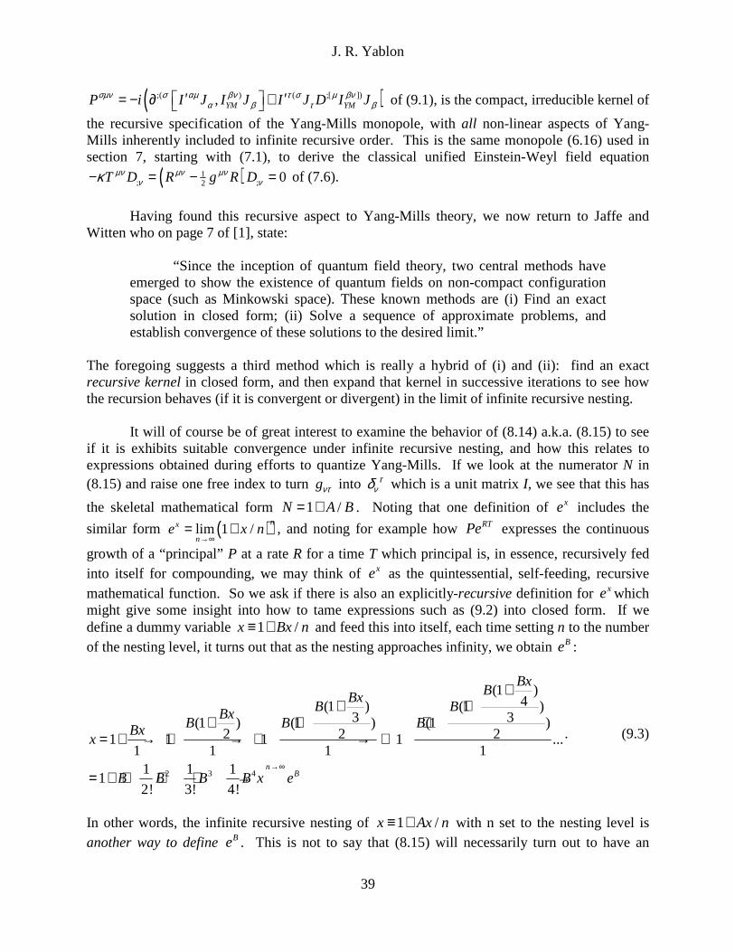
J. R. Yablon

39

( );( ) ( ;[ ]), YM YMP i I J I J I J D I Jσµν σ αµ βν τ σ µ βνα β τ β′ ′ = − ∂ + of (9.1), is the compact, irreducible kernel of

the recursive specification of the Yang-Mills monopole, with all non-linear aspects of Yang-Mills inherently included to infinite recursive order. This is the same monopole (6.16) used in section 7, starting with (7.1), to derive the classical unified Einstein-Weyl field equation

( )1; ;2 0T D R g R Dµν µν µνν νκ− = − = of (7.6).

Having found this recursive aspect to Yang-Mills theory, we now return to Jaffe and Witten who on page 7 of [1], state:

“Since the inception of quantum field theory, two central methods have emerged to show the existence of quantum fields on non-compact configuration space (such as Minkowski space). These known methods are (i) Find an exact solution in closed form; (ii) Solve a sequence of approximate problems, and establish convergence of these solutions to the desired limit.”

The foregoing suggests a third method which is really a hybrid of (i) and (ii): find an exact recursive kernel in closed form, and then expand that kernel in successive iterations to see how the recursion behaves (if it is convergent or divergent) in the limit of infinite recursive nesting. It will of course be of great interest to examine the behavior of (8.14) a.k.a. (8.15) to see if it is exhibits suitable convergence under infinite recursive nesting, and how this relates to expressions obtained during efforts to quantize Yang-Mills. If we look at the numerator N in (8.15) and raise one free index to turn gντ into τ

νδ which is a unit matrix I, we see that this has

the skeletal mathematical form 1 /N A B= + . Noting that one definition of xe includes the

similar form ( )lim 1 /nx

ne x n

→∞= + , and noting for example how RTPe expresses the continuous

growth of a “principal” P at a rate R for a time T which principal is, in essence, recursively fed into itself for compounding, we may think of xe as the quintessential, self-feeding, recursive mathematical function. So we ask if there is also an explicitly-recursive definition for xe which might give some insight into how to tame expressions such as (9.2) into closed form. If we define a dummy variable 1 /x Bx n≡ + and feed this into itself, each time setting n to the number of the nesting level, it turns out that as the nesting approaches infinity, we obtain Be :

2 3 4

(1 )4(1 ) (1 )

3 3(1 ) (1 ) (1 )2 2 21 1 1 1 ...

1 1 1 11 1 1

12! 3! 4!

nB

BxBBx

B BBxB B BBx

x

B B B B x e→∞

++ +

+ + += + → + → + → +

= + + + + →

. (9.3)

In other words, the infinite recursive nesting of 1 /x Ax n≡ + with n set to the nesting level is another way to define Be . This is not to say that (8.15) will necessarily turn out to have an

J. R. Yablon

40

exponential form, but rather to point out how a Maclaurin series for Ae may be recursively defined from the recursive kernel 1 /x Bx n≡ + where n is the nesting level. It would seem a fruitful mathematical exercise to develop similar recursive definitions for other mathematical functions via their Maclaurin series, and then, armed with those definitions, to take a fresh look at (9.2) and see if that provides further insight into understanding this recursive series and the circumstances under which this series diverges or tractably-converges, and what it looks like in truly closed form. The other very important insight to carry away from the recursive expression (9.2), in light of (9.3), which is a mathematical insight with possible physical implications is this: In (9.3) x is a “dummy” variable that gets stripped away in the infinite application of recursion. This means that in (9.2) the gauge field Gτ is the dummy variable that will get stripped away by the

recursion as the nesting reaches infinity, and that what will remain behind is the single Gτ on the

left of (9.2) expressed as an infinite recursive series with up to infinite powers of the source currents Jν . Possibly analogously, when we take a path integral, such as in QED:

( )( )( )

( )( )( )

4 212

4 2

4 2

exp

1exp exp

2 2

Z DG i d x G g m G J G

k kgd k miW J i J Jk k m

µν σ µ ν µµ µ σ ν µ

µ νµν

µ νσ

σπ

= ∂ ∂ + − ∂ ∂ −

− +

≡ = − −

∫ ∫

∫C C

, (9.4)

the gauge field Gτ is the “dummy” variable of integration, it also gets stripped away as the

integration takes place, and what is left behind is an amplitude expression with up to infinite powers of the source currents Jν .

With this in mind, using what Zee [7] in Appendix A refers to as the “central identity of quantum field theory” (we have reversed the sign for J because we are using the electrodynamic convention in which the units of charge (electrons) are negative whereas Zee uses a positive charge sign convention):

( )( ) ( )( ) ( )11 12 2exp exp / expD K V J V J J K Jφ φ φ φ φ δ δ −− ⋅ ⋅ − − ⋅ = ⋅ ⋅∫ C , (9.5)

it would be a very interesting mathematical exercise to see whether the core Gaussian integral:

( ) ( ) ( ).52 212exp 2 / exp / 2dx Ax Jx A J Aπ− − = −∫ (9.6)

can be fully reformulated in terms of a recursive function. As a start toward this, it helps to develop what may be a new mathematical notation to represent this sort of recursive nesting. Analogously to how series are summarized using the symbol 1n

∞=Σ , we shall now create an

infinite nest symbol represented by a pair of nested parenthesis 1(())n∞

= . In the function to be

J. R. Yablon

41

nested, we shall enclose the dummy variable (which was x in (9.3)) in the form (( ))x . Thus, in this (possibly new) notation, we may write (9.3) in compact form as:

( )( ) ( )( )( )11 /B

ne B x n

∞

=≡ + (9.7)

This means that the Gaussian integral (9.6) may be recursively written as:

( ) ( ) ( ) ( ) ( )( ) ( )( )2.5 .52 21

2 1exp 2 / exp / 2 2 / 1

2n

J xdx Ax Jx A J A A

Anπ π ∞

=

− − = = +

∫ (9.8)

where x (an abstracted gauge field), which is a dummy variable of integration, is what gets stripped away during the infinite recursion as a dummy variable of recursion. It is not at this point clear whether this sort of recursive analysis can be helpful in breaking through to enable an exact, analytical path integral quantization of Yang-Mills theory in closed form, but it is worthwhile to see what contributions can be made by a recursive analysis in which the physical field to be subjected to path integration is instead regarded as a dummy variable in a recursive expansion. What is absolutely clear, however, is that Yang-Mills theory, in the form of (9.1) and (9.2), forces upon us the need to analyze, understand, and better develop its recursive features, which are yet a sixth view of Yang Mills in which all of the non-linearities are expressed and developed through recursive mathematics. One should amidst this analysis, be looking for ways to analytically calculate the exact Yang-Mills path integral with the aid of the recursive kernel in (9.2) which does mirror the types of terms that get fed into the Yang-Mills path integral. In section 13, we shall do exactly that. All of the forgoing also applies to gravitation theory, which from a “gravitation gravitates” view possesses a similar sort or recursive non-linearity. It is also worth observing that the magnetic monopole (9.1), now populated with fermions (which in section 11 we will show are quarks) is really, at bottom, a non-Abelian combination of both of Maxwell’s classical equations (3.1) and (3.2) into a single equation. Specifically, the Yang-Mills electric charge equation combined with Dirac wavefunction theory via

[ ]; ;J D F D D Gν µν µ ν νµ µ γ= = = Ψ Ψ is represented in inverse form via (9.2) and then inserted into

the monopole density (3.6) to arrive at (9.1). Einstein, in his final paper [21] at page 159 points out the “surprising” finding that Maxwell’s two equations, taken together, possess a field strength 1 12z = which is the exact same strength as the equation 0Rµν = for pure geometry.

This would suggest that (9.1), which is a field equation relating all three of Jν νγ= Ψ Ψ , Pσµν

and Gµ (two sources and one gauge field) to one another, and which merges both of Maxwell’s equations together into one, will also have a strength 1 12z = interrelating its 21,2,3... 1i N= −

Abelian sources iJ ν , iP σµν and fields iG µ , and so also have the same strength as 0Rµν = .

The final, very important point to note is that because of its origin in (3.2) and (3.6) as a

Yang-Mills monopole, (9.1) contains three additive terms in index-cyclic ( )σµν configuration

of the form ;( ),YM YMI Iσ αµ βνα βγ γ ∂ Ψ Ψ Ψ Ψ , and similarly ( ;[ ])

YM YMI D Iτ σ µ βντ βγ γΨ Ψ Ψ Ψ . Further,

J. R. Yablon

42

AΨ = Ψ is an N-component column vector of 4-component Dirac spinor wavefunctions ψ for

whatever gauge group SU(N) we choose to employ. To this moment, we have been exploring Yang-Mills gauge theory in general, but have made no selection of any specific gauge group. Now that is about to change. Because Pσµν is the density of a single magnetic monopole, Pσµν

must be regarded as a system which contains these AΨ = Ψ . But by virtue of the three additive

terms, it would appear to contain three such Yang-Mills fermions Ψ . This was the source of the “three-ness” discussed at some length toward the end of section 4. Dirac-Fermi-Pauli exclusion tells us to make certain that that the fermions in each of these terms are in different eigenstates, so that this monopole system does not contain any two fermions in the same state. Because there are three additive terms, the smallest group we are permitted to choose is SU(3). By Occam’s Razor, we make this smallest permitted selection, and so do choose SU(3).

Once we choose SU(3), we place each of the now-three ψ of AΨ = Ψ , A=1,2,3 into a

distinct eigenstate. In order to discuss this, we need to name these states. So we will name them Red, Green and Blue, and denote them Rψ , Gψ and Bψ . And with that, we move from Yang-

Mills gauge theory generally, to Chromodynamics specifically. And while we start with three fermions Rψ , Gψ and Bψ which we shall soon establish may be interpreted as quarks, the

recursive nature of (9.1) via (9.2) and D iGµ µ µ= ∂ − and G I J Iτ τµ τµ τµ γ′ ′= = Ψ Ψ ensures us the

monopole system of (9.1) will be teeming with non-linear physics and many additional quarks and antiquarks and amidst a sea of gluons that arise at the first, second, thousandth, and millionth recursive order. This will all be developed in detail in section 11.

In this light, as stated in the introduction, and as we shall detail in the forthcoming development of section 11, QCD is not a theory of first principle, it is corollary theory. The theory of first principle is Maxwell’s electrodynamics as extended into non-Abelian domains by Yang-Mills gauge theory. QCD is then derived by deduction as a consequence of enforcing exclusion for the fermions contained in the non-vanishing magnetic monopoles of Yang-Mills gauge theory, and choosing a gauge group no larger than is necessary to enforce this exclusion. In the process, we fully explain why nature chooses three quarks per baryon (in the “ground” state of zero-recursive order) rather than some other number.

Now we turn to make three specific showings: First, in section 10, we shall show how

the relationship (8.14) which via YMG I Jτµ τµ≡ is contained to infinite recursive order in

monopole (9.1) via (9.2), fills the mass gap. To preview: if we set 0m= in (8.14), due the non-commuting nature of Yang-Mills theory, we still retain terms which create mass-like effects and

which, because of the specific matrix inversion ( ) 1;;D D σσ

− in (8.14), yield a mass eigenvalue

spectrum, which one expects will come to be associated with the non-zero masses of the observed mesons such as those catalogued in [22]. Second, in section 11, as has already been developed to some degree in section 4, we shall show from a more formal standpoint how and why (9.1) contains all of the expected color symmetries of a baryon, and at the same time confines its fermions (which we shall identify with quarks) and its gauge fields (which will identify with gluons), while permitting the flux of colorless quark combinations that we observe in the form of mesons. It is by this means that we shall identify the magnetic monopoles of

J. R. Yablon

43

Yang-Mills gauge theory as baryons, which naturally possess three colored quarks at the lowest recursive order and only permit a flow of mesons across their closed surfaces. Finally, in section 12 we shall examine the natural origin of chiral symmetry breaking, and particularly, of the various vector (V) and axial (A) meson states which are phenomenologically-evidenced in strong interactions. 10. The Mass Gap Solution Let us now show how the solution to the mass gap that is embedded in equation (8.14) which in the form (9.2) yields an infinite recursion. We shall develop this solution using the more “user-friendly” representation (8.15). The configuration space inverse YMI ντ in (8.15), upon expansion of each D iGµ µ µ= ∂ −

followed by reapplication of (9.2), represents all of the non-linear, recursive features of Yang-Mills theory. As we have done previously, let us now identify how much of this inverse arises strictly from the perturbations P which represent the “difference” between Yang-Mills gauge theory and an Abelian gauge theory such as Maxwell’s electrodynamics. As we did earlier with (5.10), we use the framework YM=L+P (total Yang-Mills effects are the sum of linear effects plus perturbative effects) to calculate P YM LI I Iντ ντ ντ= − , which is simply the difference between

the entire, holistic ([7], page 356) inverse (8.15) and the linear inverse (8.9). So what we shall now be studying is what Yang-Mills theory brings to the table (perturbations in the perturbative view), above and beyond what Abelian gauge theories such as electrodynamics already bring to the table. So that we can study only the impact of Yang-Mills theory separated from any impact due to spacetime curvature, we represent both of (8.9) and (8.15) in flat spacetime, and so turn the gravitationally-covariant derivatives ;σ∂ into ordinary ones σ∂ . Thus, we form:

2 2

2 2

" "

" "

P YM LI I I

D D D Dg g

m D D D D D D D D D D m

D D m m

ντ ντ ντα β α β

ν τ ν τντ ντα β σ α β β α σ α β σ α β β α σ

σ σ σ σσ σ

σ σ

∨∨

= −

∂ ∂ ∂ ∂+ ++ − ∂ ∂ + ∂ ∂ ∂ ∂ − ∂ ∂ ∂ ∂= −

+ ∂ ∂ +

.(10.1)

The ordinary derivatives in the right hand term commute and the denominators are real denominators, not matrix inverses. So the above readily reduces to (see (8.9) to (8.10) where we did the same reduction earlier):

2 2

2 2

" "

" "

P YM LI I I

D D D Dg gm D D D D D D D D D D m

D D m m

ντ ντ ντα β

ν τ ν τντ α β σ α β β α σ ντσ σ

σ σσ σ

∨∨

= −

∂ ∂+ ++ −= −+ ∂ ∂ +

. (10.2)

The term on the right, of course, is the inverse for a massive spin-1 vector field (vector boson), it is identical to what we found in (8.10), and when we convert over to momentum space, it is the same thing as the vector boson propagator up to a factor of i, LiIντ ντπ = . The QED path

J. R. Yablon

44

integration which establishes that LiIντ ντπ = , is displayed in (9.4). The term [ ]D D D D D D D D D D D Dσ α β σ α β β α σ

σ σ σ= − , which will be at the heart of the discussion to

follow, contains a succession of four covariant derivatives, and as we can see from the identities developed in section 6 and especially (6.9) and (6.17) to (6.20), this term [ ]D D D Dσ α β

σ is non-

vanishing everywhere there are non-zero perturbations as defined in (5.3) to (5.5).. Now let us return to (5.6) for two successive gauge-covariant derivatives, and write this perturbatively in momentum space in flat spacetime via i kµ µ∂ → , as

;D D k k V k k k G G k G Gµ ν µ ν µν µ ν µ ν µ ν µ ν= − + = − − − − , (10.3) which also means that: V k G G k G Gµν µ ν µ ν µ ν≡ − − − . (10.4) So we expand the various D D k k Vµ ν µ ν µν= − + in (10.2) and convert into momentum space, to obtain:

( ) ( )( ) ( )( ) ( ) ( )2

2

2

2

" "

" "

P YM LI I I

k k V k k Vg

m k k V k k V k k V k k V k k V

k k V m

k kg

mk k m

ντ ντ ντ

α β αβν τ ντ

ντ α β αβ σ σ α β αβ β β α σ ασσ σ σ σ

σ σσ σ

ν τντ

σσ

∨

∨

= −

− − +− +

− + + − − − − −=

− −

− +−

−

. (10.5)

We of course see the perturbative-only inverse 0PI ντ → if all the perturbations are

turned off, 0Vαβ → , as is to be expected. Again, we are now largely working in the perturbative view of Yang-Mills.

What we now wish to consider is this: In the full Yang Mills inverse YMI ντ in (10.5), the

2m is the Proca mass of the Yang-Mills gauge bosons, introduced by hand back in (3.3). That mass has followed us all the way through the development since, but as originally pointed out, it is a red flag mass that we want to eventually be able to zero out and – if there are massive particles to be found in the physics we are describing –be able to reintroduce in some other way without ruining the gauge invariance and renormalizability of the theory. So now, the time has come to set the Proca mass in YMI ντ to zero. But we shall leave the Proca mass as is in LI ντ to

keep one “red flag” in place as will be momentarily discussed. With setting 2 0m = in YMI ντ , the

above now reduces to:

J. R. Yablon

45

( ) ( )( )( ) ( )( ) 2

2

" "

" "

P YM LI I I

k k V k k Vk kg

gk k V k k V k k V k k V mk k V k k m

ντ ντ ντ

α β αβν τ ντ

ν τντ σ σ α β αβ β β α σ ασντσ σ σ σ

σ σ σσ σ σ

∨

∨

= −

− − +− + − +− − − − −

= −− −

. (10.6)

This means that (3.3) is now reverted to ( ); ; ;

;J g D D D D Gν µν σ µ νσ µ= − , so that the Yang-Mills

gauge bosons are now massless. This means, for example, that if our gauge group is SU(3)C, then these gauge bosons will be massless gluons.

While we are at it, let us even go a step further, by setting the now-massless gauge bosons in YMI ντ to be on mass shell, with 0k kσ

σ = (which means that the term 0k k k kβ α σσ →

because the kσ can commute since we have assumed flat spacetime to isolate the effects of Yang-Mills all by itself), while at the same time adding iε+ to the linear inverse LI ντ and also

introducing the gauge number ξ , which for 1ξ = is the Feynman gauge and for 0ξ = is the Landau gauge. This gauge number is associated with the Faddeev-Popov method and was originally developed by Feynman, see, e.g., [7] section III.4. The latter 0ξ = is the gauge of (10.6). Let us also raise the free ν index everywhere. Thus, (10.6) now becomes:

( ) ( )( ) ( ) 2

2

1" "

" "

P YM LI I I

k k V k k Vk k

V V k k k k V V V V k k mV k k m i

ν ν ντ τ τ

ν α β αβτ ντ νν

ν ττ σ αβ α β β ασ β ασ β α στσ σ σ σ

σ σσ σ

δ δ ξ

ε

∨

∨

= −

− − +− + − + −− + − +

= −− − +

. (10.7)

To simplify our consideration of LI ν

τ a bit, let us choose the Feynman gauge1ξ = which is what

transpires anyway the moment one contracts the inverse LI ντ with a current density via 0k Jτ

τ = ,

see (8.11). Thus, (10.7) now becomes:

( ) ( )( )

2

" "

" "P YM L

k k V k k V

V V k k k k V V V V k kI I I

V k k m i

ν ν α β αβτ τν

τ σ αβ α β β ασ β ασ β α σ νσ σ σ σν ν ν τ

τ τ τ σ σσ σ

δδ

ε

∨

∨

− − +− +

− + − + −= − = −− − +

.(10.8)

Now we arrive at the point: Even after we set the Proca mass to zero to keep the Yang-Mills gauge bosons massless and preserve renormalizability, and even after we further set those zero-mass gauge bosons to be on-shell, so long as the perturbations Vαβ and V σ

σ are not zero –

which means that so long as Yang-Mills theory is doing something more than Abelian gauge theory – the inverse YMI ντ remains entirely finite and well-behaved. We do not need the Proca

mass at all, and we do not even need iε+ to avoid the pole that occurs in LI ντ when 2 0k k mσ

σ − = (or when 0k kσσ = with 2 0m = ). Referring to (10.4), the

J. R. Yablon

46

( ) ( )1 11/ " "V V k G G k G Gσ σ σ σ σ

σ σ σ σ σ− −

= = + − term keeps YMI ντ well-behaved in exactly the

same way that 2k k m iσσ ε− + keeps the linear LI ντ well-behaved. But – at the heart of the

matter – ( ) ( )1 11/ " "V V k G G k G Gσ σ σ σ σ

σ σ σ σ σ

− −= = + − is an NxN matrix inverse that arises with

no artifice from the essential non-linear core of Yang-Mills theory. In contrast, in the linear inverse LI ν

τ , in the denominator 2k k m iσσ ε− + , the 2m is a renormalization-destroying Proca

mass which has us asking why, for example, the strong interaction can be a short range interaction even though its gauge boson masses are zero which means we cannot introduce a Proca mass even though we need a Proca mass to make the strong interaction short range and make the inverse / propagator LiIντ ντπ = non-infinite. And in further contrast, iε+ is another

artifice introduced by hand, to avoid the pole of an on-shell boson. Similarly, as we even saw following (8.12), the moment we set 2 0m = , the numerator term 2/k k mν τ → ∞ in LI ντ , unless

the spacetime is curved. Here, where we are considering Yang-Mills alone and have removed any effects of gravitational curvature, the corresponding “denominator” in (10.7),

( )( ) 1

V V k k k k V V V V k kσ αβ α β β ασ β ασ β α σσ σ σ σ

−− + − + , plays the analogous role to the spacetime

curvature , and is perfectly well-behaved so long as the perturbations Vαβ and V σσ are not zero,

which is exactly what Yang-Mills theory is all about. So, now, to the mass gap: The Klein Gordon equation (5.1) for a massless scalar field φ with gauge symmetry, plus a hand-added Proca mass term for a vector boson with mass, has an associated Lagrangian density (every Lagrangian density is multiplied by 2 in Yang-Mills because of the generator normalization ( ) 1

2i j ijTr λ λ δ= , see (2.6)):

( ) ( ) ( )† 2 2

2

D D m G G iG iG m G G

i G i G G G m G G

µ µ µ µ µµµ µ µ µ

µ µ µ µ µµ µµ µ µ

φ φ φ φ

φ φ φ φ φ φ φ φ

←

← ←

= − = ∂ − ∂ − −

= ∂ ∂ − ∂ − ∂ − −

L

(10.9)

Above, we use ( )( )†iG iGµµ µ µφ φ

← ∂ − = ∂ −

due to the hermicity of the gauge fields i iG Gµ µλ=

which is in turn due to †i iλ λ= for the Yang-Mills generators, and we also use a left-operating

µ←∂ . (While we are here, contrast ( )†

D Dµµφ φ above to one possible use of the Einstein-Weyl

equation (7.6) so as to operate on a scalar field, namely, ( )1;2 0R g R Dµν µννϕ− = .) Although the

only ingredients we start with in (10.9) are a scalar φ for which we take the gauge-covariant

derivativeDµφ , we end up with a term G Gµµφ φ . When we then expand the scalar around the

vacuum using a Higgs fields in the form ( ) ...v h xφ = + + and rescale G gGµ µ→ to explicitly

show the gauge coupling, this gauge-created term:

J. R. Yablon

47

( ) ( ) ( ) ( )22 2 2 2... ... 2 ...g G G g v h G G v h vg G G g vh h G Gµ µ µ µµ µ µ µφ φ− = − + + + + = − − + + (10.10)

reveals the term ( )2vg G Gµ

µ− . So now (10.9) contains ( )2 2vg G G m G Gµ µµ µ− − . But the term

2m G Gµµ− was introduced by hand with a Proca mass and it ruins the gauge symmetry. The term

( )2vg G Gµ

µ− , on the other hand, is a direct result of the gauge symmetry. In fact, the gauge

symmetry would be ruined if we did not have this term. So we remove the Proca mass (set it to

zero) and in its place we regard the term ( )2vg G Gµ

µ− to represent the massive boson and vg to

represent the mass of the boson. The experimental confirmation of electroweak theory, of

course, validates this result, and at the same time, by using ( )2vg G Gµ

µ− rather than 2m G Gµµ as

the boson mass term, we keep the gauge theory remains renormalizable. The benefit of having 2m G Gµ

µ− in (10.9) is that it represents an “anticipated” mass against which we compare the

emergent ( )2vg G Gµ

µ− to identify the renormalizable mass vg in lieu of the Proca mass m.

The exact same sort of thing is happening in (10.8). Based on what we know from Abelian gauge theory, we have come to expect that massive vector bosons will have a propagator

LiIντ ντπ = . The term LI iντ ντπ= − in (10.8) is completely analogous to the term 2m G Gµµ in

(10.9). Each contains a hand-added, renormalization-destroying, “anticipated” Proca mass. And (10.8) does (10.9) one better, because it also has a hand-added iε+ to ensure that the world does not come to an end when a boson is on-shell. But in strong interaction theory, we expect the gauge bosons to be massless. Were we to set m=0 in the LI ντ of (10.7) before we gauged out this

term with 1ξ = in (10.8), everything would blow up. Were we to set the boson on-shell in LI ντ

and not use iε+ added in (10.7), everything would blow up. But the compete inverse in Yang-Mills theory is YMI ντ , not LI iντ ντπ= − . So YMI ντ , not LI ντ , is the inverse in which we should set

m=0. By keeping m explicitly in LI ντ , we keep the “red flag” of what is “anticipated” so that we

can see how this anticipated mass arises from YMI ντ , just as when we kept the Proca mass in

(10.9). And while we are at it, if we want the gauge bosons to be on-shell, YMI ντ is also the

inverse in which we should set 0k kσσ = . In (10.7) we have already done all of this. The mass is

zero, the bosons are on-shell, and we have done nothing by hand that is artificial. And what great catastrophe has befallen YMI ντ in (10.7)? Absolutely none! This remains a completely

finite, well-behaved matrix expression, so long as 0Vασ ≠ and 0V σσ ≠ . But where and how,

exactly, mathematically, do we fill the mass gap? This is where the matrix expressions and the inverses come in. Written out expressly in terms of matrices and inverses with matrix indexes AB, (10.8) really says:

J. R. Yablon

48

( ) ( )( ) ( )( )( )( ) ( )

11

2/

P AB YM AB L AB

AB

AB

I I I

k k V V V k k k k V V V V k k k k V V

k k m i

ν ν ντ τ τ

ν ν ν σ αβ α β β ασ β ασ β α σ α β αβ στ τ τ σ σ σ σ σ

ν στ σ

δ

δ

δ ε δ

−−

= − =

− + − − + − + − + −

− − − +

.(10.11)

We have taken special pains to make explicit, the NxN matrix structure, noting that YM ABI ν

τ is a

complete, non-commuting, rather complicated NxN Yang-Mills matrix for SU(N), and that

( )2/LI k k m iν ν στ τ σδ ε= − − + is not a Yang-Mills matrix . Rather, when we subtract LI ν

τ from

PI ντ , we must put LI ν

τ (which is related to the linear propagator by LiIντ ντπ = ) into the diagonal

positions of the Yang-Mills unit matrix ABδ , thus forming L ABI ντδ .

But (10.11) is in the form of an eigenvalue equation for the matrix YM ABI ν

τ , with

LI iν ντ τπ= − representing the eigenvalues of YM ABI ν

τ . So if we use this to operate on any Yang-

Mills column vector BV , then LI iν ντ τπ= − will represent the eigenvalues, i.e., the propagator

observables, of the matrix YM ABI ντ . But we don’t even need to posit a vector BV because we may

obtain these eigenvalues directly from (10.11) via the eigenvalue equation ( )det 0M I M Iλ λ− = − = which uses the determinant of a matrix M to compute its eigenvalues

λ. For (10.11) this eigenvalue equation takes the form:

0P AB YM AB L ABI I Iν ν ντ τ τδ= − = . (10.12)

That is it! This is the mass gap solution! Once we deduce a non-zero eigenvalue LI iν ν

τ τπ= −

via the above from some perturbations 0Vασ ≠ and 0V σσ ≠ in YM ABI ν

τ , we then know that the

observable, anticipated mass m will be related to this by:

2 LI ik k m i

νν ντ

τ τσσ

δ πε

− = = −− +

. (10.13)

In this way, we may deduce both the mass m and, if an eigenvalue LI ν

τ is a complex number with

an imaginary component (which it may be because the iλ generators systemically generate

complex numbers once one takes a matrix inverse such as ( ) 1V σ

σ−

), the imaginary magnitude

iε+ corresponds not to the mass – but to a half-life. (See, e.g., [23], page 150.) So, we now turn directly to the mass gap problem in [1], which states at page 3:

“. . . for QCD to describe the strong force successfully . . . It must have a “mass gap;” namely there must be some constant ∆ > 0 such that every excitation of the vacuum has energy at least ∆,”

J. R. Yablon

49

and which at page 6 then sets forth the problem:

“Prove that for any compact simple gauge group G, a non-trivial quantum Yang–Mills theory exists on 4

� and has a mass gap > 0 . . . namely there must be some constant ∆ > 0 such that every excitation of the vacuum has energy at least ∆ . . .”

The solution to the mass gap is as follows: For a compact simple gauge group G which

may be “any” gauge group SU(N) with 2N ≥ and generators iλ and gauge bosons i iG Gµ µλ= , the complete, holistic, non-Abelian, non-linear classical inverse YMI ντ associated with these

gauge fields Gµ and defined by YMG I Jτµ τµ≡ , with a hand-added Proca mass m, will be the

YMI ντ included in (10.1) generally, and included in (10.2) in flat spacetime. As pointed out

already, the term [ ]D D D Dσ α βσ in (10.2) is non-vanishing. To maintain the renormalizability of

gauge group G, we must set this Proca mass to zero, as we do in (10.6). This means that the gauge bosons are now massless. If one takes the gauge group to be SU(3)C then the gauge bosons are gluons and these gluons are now massless. But we are in no way restricted to SU(3)C or to any other specific gauge group G. These results apply to “any compact simple gauge group G.” For good measure, though not essential, we even place the gauge bosons on-shell as in (10.7).

Now that the gauge bosons are massless, the question becomes how “there must be

constant ∆ > 0 such that every excitation of the vacuum has energy at least ∆.” The “excitations of the vacuum,” in Yang-Mills, are the perturbations V k G G k G Gµν µ ν µ ν µ ν= + − of (10.4). For every such perturbation / excitation, 0V µν ≠ and 0V σ

σ ≠ , by definition. Wherever 0 V µν< < ∞

and 0 V σσ< < ∞ , the matrix YMI ντ will be finite and well behaved, and the eigenvalues of YMI ν

τ

obtained through the eigenvalue equation (10.12) will be finite and non-zero and given by LI ντ .

These eigenvalues, which are physical observables related to the linear propagator by

LI iν ντ τπ= − , may, in the process, also be complex. These eigenvalues in turn, are related to

boson masses and lifetimes via (10.13). This means that the “anticipated” mass m in (10.13) will also be non-zero, that is, will have a value > ∆ where ∆ is some non-zero value, notwithstanding the fact that we have set m=0 in (10.6). And because this mass is contained within an inverse

LI ντ which is an eigenvalue of YMI ν

τ , this mass is deducible (as are possible non-infinite

lifetimes) via (10.13). This works for any compact simple gauge group G, which is to say, at no point in this completely general development have we assumed or needed to assume one particular group over any other. (Though as we have pointed out toward the end of the last section based on (10.1), Yang-Mills monopoles give us reason for regarding SU(3) as a particularly important group, which will be developed further in the next section.)

The mass m which we did maintain as a red flag in LI ντ in (10.13) is similar to 2m G Gµ

µ

which we maintained as a red flag in (10.9). It is a hand-added version of a mass that we observe in the physical world but may not put into the theory by hand without ruining the renormalizability of the theory. So we look for ways for this “anticipated” mass to be revealed

J. R. Yablon

50

by the theory in some other way. In (10.12), this mass which fills the mass gap is revealed in the theory because the excitations in (10.11) give this mass non-zero eigenvalues via (10.13) and the non-zero eigenvalues LI ν

τ are the reciprocals of what then becomes a finite, non-zero, possibly

complex, well-behaved 2k k m iσσ ε− + , even though the gauge boson masses have been set to

zero. If we set 0k kσσ = , then these eigenvalues LI ν

τ are simply the reciprocals of 2m iε− + ,

which is a pure mass number with infinite lifetime (stable particle) for real eigenvalues, and a pure mass number and finite lifetime (unstable particle) for complex eigenvalues. The mass gap is filled, and we then have the basis for explaining why Yang-Mills interactions – most notably the strong interaction – are able to have a short range which requires massive vector bosons and at the same time have gauge bosons which are massless. The mass gap is filled because (10.12) “reveals” a non-zero mass in the inverse (10.13) without ever introducing that mass by hand, in exactly the same way that (10.10) reveals a non-zero mass in the Lagrangian density (10.9) without ever introducing that mass by hand. Having now filled the mass gap, we return to show why it is that the Yang-Mills monopoles (9.1) have all the chromodynamic color symmetries required of a baryon, and at the same time confine their quarks and its gauge fields, while permitting the flux of colorless quark combinations that we observe in the form of mesons. Given that the mass gap is now filled, this in turn would mean that the nuclear forces associated with these monopole baryons have short range. And, as we shall see, the specific massive particles which emerge in the mass gap solution (10.12), physically, are the mesons observed to be the mediators of strong interactions. 11. Populating Yang-Mills Monopoles with Fermions to Reveal that Yang-Mills Monopoles have the Chromodynamic and Confinement Symmetries of Baryons and Emit and Absorb Objects with the Chromodynamic Symmetries of Mesons Let us return to the monopole (9.1) which we have populated with the fermion sources Ψ from which its gauge fields arise. As we did in the last section, we write the inverses in the form YM L PI I Iντ ντ ντ= + to show the sum of the linear plus perturbative contributions to the

complete Yang-Mills inverse YMI ντ . And, we stay in flat spacetime and thereby set all

spacetime-covariant derivatives to ordinary derivatives, ;µ µ∂ → ∂ . And, we keep in mind that

ABP Pσµν σµν= is an NxN matrix for SU(N). So, substituting YM L PI I Iντ ντ ντ= + into (9.1) yields:

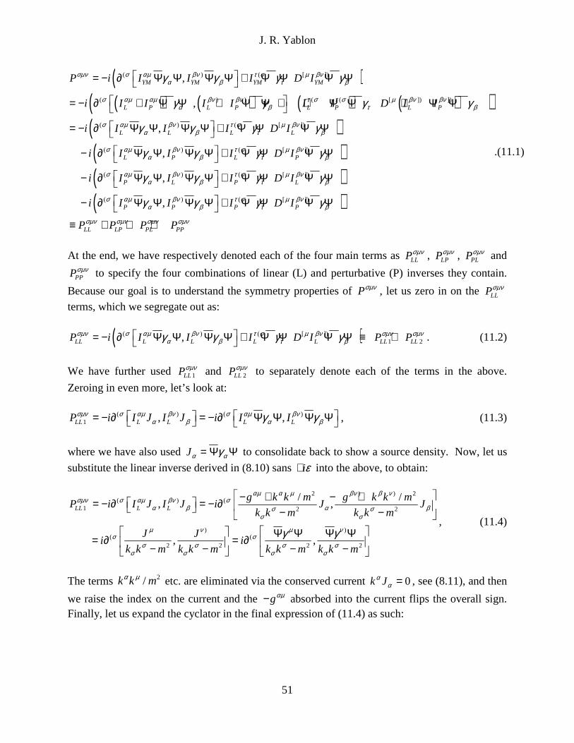
J. R. Yablon

51

( )( ) ( ) ( ) ( )( )

( )

( ) ( [ ])

( ) ) ( ( [ ]) ])

( ) ( [ ])

(

,

,

,

,

YM YM YM YM

L P L P L P L P

L L L L

L

P i I I I D I

i I I I I I I D I I

i I I I D I

i I I

σµν σ αµ βν τ σ µ βνα β τ β

σ αµ αµ βν βν τ σ τ σ µ βν βνα β τ β

σ αµ βν τ σ µ βνα β τ β

σ αµα

γ γ γ γ

γ γ γ γ

γ γ γ γ

γ

= − ∂ Ψ Ψ Ψ Ψ + Ψ Ψ Ψ Ψ

= − ∂ + Ψ Ψ + Ψ Ψ + + Ψ Ψ + Ψ Ψ

= − ∂ Ψ Ψ Ψ Ψ + Ψ Ψ Ψ Ψ

− ∂ Ψ Ψ( )( )( )

) ( [ ])

( ) ( [ ])

( ) ( [ ])

,

,

P L P

P L P L

P P P P

LL LP PL PP

I D I

i I I I D I

i I I I D I

P P P P

βν τ σ µ βνβ τ β

σ αµ βν τ σ µ βνα β τ β

σ αµ βν τ σ µ βνα β τ β

σµν σµν σµν σµν

γ γ γ

γ γ γ γ

γ γ γ γ

Ψ Ψ + Ψ Ψ Ψ Ψ

− ∂ Ψ Ψ Ψ Ψ + Ψ Ψ Ψ Ψ

− ∂ Ψ Ψ Ψ Ψ + Ψ Ψ Ψ Ψ

≡ + + +

.(11.1)

At the end, we have respectively denoted each of the four main terms as LLPσµν , LPPσµν , PLPσµν and

PPPσµν to specify the four combinations of linear (L) and perturbative (P) inverses they contain.

Because our goal is to understand the symmetry properties of Pσµν , let us zero in on the LLPσµν

terms, which we segregate out as:

( )( ) ( [ ])1 2,LL L L L L LL LLP i I I I D I P Pσµν σ αµ βν τ σ µ βν σµν σµν

α β τ βγ γ γ γ = − ∂ Ψ Ψ Ψ Ψ + Ψ Ψ Ψ Ψ ≡ + . (11.2)

We have further used 1LLPσµν and 2LLPσµν to separately denote each of the terms in the above.

Zeroing in even more, let’s look at:

( ) ( )1 , ,LL L L L LP i I J I J i I Iσµν σ αµ βν σ αµ βν

α β α βγ γ = − ∂ = − ∂ Ψ Ψ Ψ Ψ , (11.3)

where we have also used Jα αγ= Ψ Ψ to consolidate back to show a source density. Now, let us

substitute the linear inverse derived in (8.10) sans iε+ into the above, to obtain:

2 ) ) 2( ) (

1 2 2

) )( (

2 2 2 2

/ /, ,

, ,

LL L L

g k k m g k k mP i I J I J i J J

k k m k k m

J Ji i

k k m k k m k k m k k m

αµ α µ βν β νσµν σ αµ βν σ

α β α βσ σσ σ

µ ν µ νσ σ

σ σ σ σσ σ σ σ

γ γ

− + − + = − ∂ = − ∂ − −

Ψ Ψ Ψ Ψ= ∂ = ∂ − − − −

, (11.4)

The terms 2/k k mα µ etc. are eliminated via the conserved current 0k Jα

α = , see (8.11), and then

we raise the index on the current and the gαµ− absorbed into the current flips the overall sign. Finally, let us expand the cyclator in the final expression of (11.4) as such:

J. R. Yablon

52

1 2 2 2 2 2 2

[ ] [ ] [ ]

2 2 2 2

, , ,

1

LLP ik k m k k m k k m k k m k k m k k m

ik k m k k m k k m k k m

µ ν ν σ σ µσµν σ µ ν

σ σ σ σ σ σσ σ σ σ σ σ

µ ν ν σ σ µσ µ ν

σ σ σ σσ σ σ σ

γ γ γ γ γ γ

γ γ γ γ γ γ

Ψ Ψ Ψ Ψ Ψ Ψ Ψ Ψ Ψ Ψ Ψ Ψ= ∂ + ∂ + ∂ − − − − − −

Ψ ΨΨ Ψ Ψ ΨΨ Ψ Ψ ΨΨ Ψ= ∂ + ∂ + ∂ − − − −

,(11.5)

where, for example, we compact [ ]µ ν µ ν ν µγ γ γ γ γ γΨ ΨΨ Ψ = Ψ ΨΨ Ψ − Ψ ΨΨ Ψ . Now, let’s develop the above in some depth. The development to follow parallels sections 2, 3 and 5 of [13], but streamlines and simplifies that development considerably and, perhaps more importantly, puts that development in the overall context of the complete set of non-linear behaviors which are the hallmark of Yang-Mills gauge theory. To start, we note the spin sum relationship which is often normalized such that

2N m= Ε + . Here, we shall not use this normalization but will use the spin sum prior to normalization which is (see, e.g., [23] exercise 5.9):

( )2

spins

NUU p m

E m= +/+∑ . (11.6)

Also seeing the emergent UUΨΨ = in each of the three terms in (11.5), we take the UUΨΨ = in all three of these terms in (11.5), and then use (11.6) to write:

( ) ( ) ( )[ ] [ ] [ ]2

1 2 2 2 2

1LL

p m p m p mNP i

k k m E m k k m k k m k k m

µ ν ν σ σ µσµν σ µ ν

σ σ σ σσ σ σ σ

γ γ γ γ γ γ Ψ + Ψ Ψ + Ψ Ψ + Ψ/ / /= ∂ + ∂ + ∂ − + − − − (11.7)

Next, we keep in mind that the fermion propagator

( )( ) ( ) 1

2

p m p mp m

p p m p m p mττ

−+ +/ /= = −/− + −/ /, (11.8)

while also noting the appearance of ( ) ( )2/p m k k mτ

τ+ −/ throughout (11.7) which is very similar

in form to the first expression in (11.8). So, if we can find some rationale (see section 3 of [13]) to associate the kτ with pτ which is the four-momentum of the fermion, then we will have established that there are propagating fermion wavefunctions populating the monopole term

1LLPσµν . Observing that ( )21/ k k mττ − represents propagation for a Proca-massive vector boson

with three degrees of freedom and that fermions have four degrees of freedom, we shift one degree of freedom from the leading ( )21/ k k mτ

τ − over to the fermions by setting m=0 to turn

that leading term into a massless boson propagator. That is, for each term in (11.7), we shift:

( ) ( )[ ] [ ]

2 2 2

1 1p m p m

k k m k k m k k p p m

α β α βγ γ

τ τ τ ττ τ τ τ

ψγ γ ψ ψγ γ ψ+ +/ /∂ ⇒ ∂− − −

. (11.9)

J. R. Yablon

53

and now take pτ to represent the fermion four-momentum. It should be clear that both parts of (11.9) contain a total of six degrees of freedom; they have just been shifted from a 3+3 to a 2+4 configuration not dissimilarly to how a degree of freedom is shifted from a Higgs scalar to a massless gauge boson to create massive vector bosons using the Goldstone mechanism. Thus, following this shifting of degrees of freedom, (11.7) becomes:

( ) ( ) ( )[ ] [ ] [ ]2

1 2 2 2

1LL

p m p m p mNP i

k k E m p p m p p m p p m

µ ν ν σ σ µσµν σ µ ν

σ σ σ σσ σ σ σ

γ γ γ γ γ γ Ψ + Ψ Ψ + Ψ Ψ + Ψ/ / /= ∂ + ∂ + ∂ + − − − (11.10)

If we now normalize such that ( )2N E m k kσσ= + , then via (11.8) we can reduce (11.10) to:

( )( ) ( )( ) ( )( )( )( )( ) ( )( ) ( )( )( )

1 1 1[ ] [ ] [ ]1

1 1 1[ ] [ ] [ ]1 2 31 2 3

LLP i p m p m p m

i p m p m p m

σµν σ µ ν µ ν σ ν σ µ

σ µ ν µ ν σ ν σ µ

γ γ γ γ γ γ

γ γ γ γ γ γ

− − −

− − −

= ∂ Ψ − Ψ + ∂ Ψ − Ψ + ∂ Ψ − Ψ/ / /

≡ ∂ Ψ − Ψ + ∂ Ψ − Ψ + ∂ Ψ − Ψ/ / /(11.11)

which contains three additive terms each containing a propagating fermion wavefunction. But in the bottom line above, we resume the development toward the end of section 9 where we noted that because Pσµν is the density of a single magnetic monopole, Pσµν must be regarded as a system which contains these AΨ = Ψ , with 1...A N= for SU(N). Since each of the three terms

in (11.11) represents a fermion propagating within the 1LLPσµν system, in an important step, we

designate (define) each term as containing a distinct eigenstate 1Ψ , 2Ψ , 3Ψ of the SU(N)

wavefunction AΨ = Ψ , 1...A N= . Specifically, Dirac-Fermi-Pauli exclusion tells us to make

certain that the fermions in each of these three terms are in different eigenstates. Thus, as already stated, because there are three additive terms, the smallest group we are permitted to choose is SU(3), and by Occam’s Razor, we make this smallest permitted selection, and so do choose SU(3). So let us now implement this. As already stated at the end of section 9, once we choose SU(3), we place each of the now-three ψ of AΨ = Ψ , A=1,2,3 into a distinct eigenstate. In order to discuss this, we need to

name these states. So we will name them Red, Green and Blue, and denote them Rψ , Gψ and

Bψ . The generators are ; 1,2,3...8i iλ = , the eight gauge bosons are i iG Gµ µλ= , and the three

fermion eigenstates are Rψ , Gψ and Bψ . Specifically, we define these eigenstates in (11.11) as:

8 3 8 3 8 31 1 1 1 11 2 32 23 2 3 2 3

0 0

; 0 0 ; ; ; ; 0

0 0

R

G

B

ψλ λ λ λ ψ λ λ

ψ

Ψ ≡ = = = Ψ ≡ = − = = Ψ ≡ = − = − =

. (11.12)

J. R. Yablon

54

This, together with having set m=0 in (10.6), means that the i iG Gµ µλ= may now be interpreted not just as generalized gauge bosons, but specifically, as the bi-colored massless gluons of chromodynamics. It also means that we may construct:

1 2 31 2 3

0 0 00 0 0 0 0

0 0 0 ; 0 0 ; 0 0 0

0 0 0 0 0 0 0 0

RR

GG

BB

ψ ψψ ψ

ψ ψ

Ψ Ψ = Ψ Ψ = Ψ Ψ =

. (11.13)

We then use (11.13) to display the explicit 3x3 matrix character of 1 1LL LL ABP Pσµν σµν= of

(11.5) with successive 1Ψ , 2Ψ , 3Ψ assigned as in (11.11) to each of the three terms as such:

[ ]

2

[ ]

1 2 2

[ ]

2

0 0

10 0

0 0

R RR R

G GG GLL AB

B BB B

k k m

P ik k m k k m

k k m

µ νσ

σσ

ν σσµν µ

τ στ σ

σ µν

σσ

ψ γ ψ ψ γ ψ

ψ γ ψ ψ γ ψ

ψ γ ψ ψ γ ψ

∂ − = ∂

− − ∂ −

.(11.14)

Then, repeating the same steps that brought us from (11.5) to (11.11), we may turn this into:

( )( )( )( )

( )( )

1[ ]

1[ ]1

1[ ]

0 0

0 0

0 0

R R

GLL AB G

B B

p m

P i p m

p m

σ µ ν

σµν µ ν σ

ν σ µ

ψ γ γ ψ

ψ γ γ ψ

ψ γ γ ψ

−

−

−

∂ −/

= ∂ −/ ∂ −/

.(11.15)

The trace equation 1 1Tr LL LL AAP Pσµν σµν= is then easily deduced to be:

( )( ) ( )( ) ( )( )( )1 1 1[ ] [ ] [ ]1Tr R G BLL R G BP i p m p m p mσµν σ µ ν µ ν σ ν σ µψ γ γ ψ ψ γ γ ψ ψ γ γ ψ− − −= ∂ − + ∂ − + ∂ −/ / / .(11.16)

This is now the fully-developed Yang-Mills magnetic monopole term 1Tr LL ABPσµν ,

populated with three colored quarks, and it is formally equivalent to [5.5] of [13]. There are of course other terms that we see in (11.1) and (11.2), but we are working with this specific term because it most clearly displays the chromodynamic symmetries of the monopole Pσµν . And, although we are working with the one term 1Tr LL ABPσµν out of the eight terms in (11.1), the

assignment (11.12) is systemic: with (11.12), every single Ψ in the complete monopole Pσµν of (11.1) has been turned into an SU(3) column vector with three color eigenstates.

J. R. Yablon

55

If we now associate each color wavefunction with the spacetime index in the related σ∂ operator in (11.16), i.e., R~σ , G~µ and B~ν , and keeping in mind that 1Tr LLPσµν is

antisymmetric in all spacetime indexes, we may express this antisymmetry with wedge products as [ ] [ ] [ ]~ , , ,R G B R G B G B R B R Gσ µ ν∧ ∧ ∧ ∧ = + + . This is the exact colorless

wavefunction that is expected of a baryon. Indeed, the antisymmetric character of the spacetime indexes in a magnetic monopole should have been a good tipoff that magnetic monopoles would naturally make good baryons. We now may assert that this Yang-Mills monopole has the exact colorless antisymmetric QCD symmetry required of a baryon.

Furthermore, if we apply Gauss’ / Stokes’ theorem to (11.16) and also include from (4.3)

in trace form the finding that 2Tr 3 Tr ,G G G dx dxµ νµ ν = ∫∫ ∫∫� � , we find that:

( ) ( ) ( )( )2

1 1 11

1 1 1[ ] [ ] [ ]

Tr Tr Tr 3 Tr ,LL LL LLLL

R G BR G B

P F i G i G G dx dx

i p m p m p m dx dx

µ νµ ν

µ ν µ ν µ νµ νψ γ γ ψ ψ γ γ ψ ψ γ γ ψ− − −

= = − = −

= − + − + −/ / /

∫∫∫ ∫∫ ∫∫ ∫∫

∫∫

� � �

�

. (11.17)

What is the color wavefunction for the 3 ,i G Gµ ν − entities? By inspection, BBGGRR ++ .

But this is the colorless symmetric wavefunction of a meson! So quarks do not net flow in and

out of closed two-dimensional surfaces surrounding 1LLP , except in the colorless BBGGRR ++

combination of a meson! In this way, (11.17) validates the suspicion expressed at the end of section 4 that the appearance of a “3” in front of ,G Gµ ν has something to do with there being

three colors of quark inside the magnetic monopole with interactions mediated by mesons. Of course, (11.17) does beg the question of what flows in and out of the complete monopole (11.1), because (11.17) only considers the term 1LLP . So if we go back to (11.1) to

apply Gauss’/Stokes’ theorem, we obtain:

( [ ]),YM YM YM YMi P I I dx dx I D I dx dx dxαµ βν τ σ µ βνα β µ ν τ β σ µ νγ γ γ γ = Ψ Ψ Ψ Ψ + Ψ Ψ Ψ Ψ ∫∫∫ ∫∫ ∫∫∫� . (11.18)

The first term in (11.1), because of the lead (σ∂ in (11.1), is fully integrable via Gauss’/Stokes theorem. The second term in (11.1) is not integrable, and so it tells us about all of the physics that is confined inside the overall volume of the monopole. But the point made by (11.17), is

that whatever does flow across a closed surface pursuant to ),YM YMI I dx dxαµ βνα β µ νγ γΨ Ψ Ψ Ψ∫∫� in

the (11.18), will have the color wavefunction BBGGRR ++ of a meson! So returning to the MIT bag model as discussed in section 4, we now see that for the

magnetic monopole (11.1) with surface flux shown in the ),YM YMI I dx dxαµ βνα β µ νγ γΨ Ψ Ψ Ψ∫∫� term in

(11.18), 1) the color wavefunction is that of a baryon, namely [ ] [ ] [ ], , ,R G B G B R B R G+ + ; 2)

from (4.4) and (4.5), Gluons 0=∫∫� ; 3) from (11.17), Mesons 0≠∫∫� and 4) Quarks=0∫∫�

J. R. Yablon

56

except in the colorless combination BBGGRR ++ of a meson. Thus, on a formal basis, with the MIT Bag Model telling us to look at what flows and does not flow across the surface of any theoretical entity proposed to be a baryon, and we see that the Yang-Mills magnetic monopole has precisely the formal color symmetries and boundary flows required for a baryon.

Again, on page 3 of [1], Jaffe and Witten note that QCD:

“. . . must have “quark confinement,” that is, even though the theory is described in terms of elementary fields, such as the quark fields, that transform non-trivially under SU(3), the physical particle states—such as the proton, neutron, and pion—are SU(3)-invariant.”

Equation (11.16) shows how the magnetic monopoles of Yang-Mills, with an

antisymmetric color wavefunction [ ] [ ] [ ], , ,R G B G B R B R G+ + , are indeed SU(3) invariant,

notwithstanding that the individual fermion eigenstates transform non-trivially under SU(3). This makes the monopoles well-suited to represent the physical particle states such as protons and neutrons, and makes the fermion eigenstates well-suited to represent quark fields. We further see from (11.17) that all the flux across a closed surface of the monopole has the

symmetric color wavefunction BBGGRR ++ which is also SU(3) invariant. Consequently, the physical particle states which the spacetime geometry does permit to net flow across closed surfaces are well-suited to represent mesons including the pion. And in the process, QCD itself is fully reproduced. But again, QCD is not a theory of first principle, but rather a corollary theory derived by deduction from Maxwell’s electrodynamics as extended into non-Abelian domains by Yang-Mills gauge theory. But in the process, we solve confinement and the mass gap and come to understand symmetric colorless meson flow.

Of course, if we wish to associate these magnetic monopoles with physical baryons, we still need to make them topologically stable and see how to use them to represent protons and neutrons which are the most important baryons, see section 6 through 8 of [13], and we need to calculate their energies to see if they make sense in relation to empirical data, see sections 11 and 12 of [13] which shows how the energies calculated from the linear-linear field strength 1LLF in

1Tr LLF∫∫� in (11.17) appear to track very closely with empirical nuclear binding energies, see

also [24]. Insofar as topological stability, we simply note that the trace equation (11.16) is non-vanishing, but that ( )Tr Tr 0i i

ABP Pσµν σµνλ= = if we regard the gauge group as SU(3), because

all of iλ are traceless. In other words, if we assume the simple group SU(3), the left and right sides of (11.16) do not match up because one side is traceless and the other is not. It is on this basis that we introduce the product group SU(3)C×U(1)B-L, and then obtain the monopole (11.16) (and generally, (11.1)) from the spontaneous symmetry breaking of larger SU(4) gauge groups with a B L− (baryon minus lepton number) generator along the lines laid out by Weinberg in [25] at 442 and [12] at 472-473, which in view of [26] Section 12.2.2 and [27] yields the quantum numbers required to turn these monopole baryons into proton and neutrons and ensure that they are topologically stable. These details of all of this are in sections 6 through 8 of [13], and fully apply to the development here with little if any elaboration or modification needed.

J. R. Yablon

57

12. Chiral Symmetry Breaking Referring back to Jaffe and Witten at page 3 of [1], in section 10 we showed how Yang-Mills theory leads to a “mass gap” notwithstanding having massless gauge gluons, and in section 11 we demonstrated “quark confinement” of all but the color-neutral meson combinations

BBGGRR ++ . Now let us briefly explore the origins of “chiral symmetry breaking,” which is the third leg of the mass gap problem In (11.17) we identified the mesons which flow in and out of the magnetic monopoles P. And in (11.16) we showed how these P, by virtue of their [ ] [ ] [ ], , ,R G B G B R B R G+ + color

wavefunctions and the net flow only of mesons and nothing else, may be interpreted as baryons. Let us now rewrite (11.17) for the meson flow in and out of the monopole baryons with

CC RR GG BB≡ + + representing a compacting (C=Color, not charge conjugation) of the three additive terms into a single shorthand term, as:

( )( ) ( )[ ]1[ ]

1 2 2

[ ]

2 2 2 2

Tr

2

C CCLL C

C CC C

p mP i p m dx dx i dx dx

p m

i p dx dx m dx dxp m p m

µ νµ ν

µ ν µ ν

µ α ν µν

α µ ν µ ν

ψ γ γ ψψ γ γ ψ

ψ γ γ γ ψ ψ σ ψ

− +/= − = / −

= + − −

∫∫∫ ∫∫ ∫∫

∫∫ ∫∫

� �

� �

. (12.1)

This also makes use of ( ) ( ) ( )1 2 2/p m p m p m−− = + −/ / . In the second line we separate the two

additive terms that emanate from p m+/ while applying p p ααγ=/ and expressly introducing the

Dirac bilinear 12 ,iµν µ νσ γ γ = . Now let’s look at what these two terms represent.

The latter term for which the core structure is C Cdx dxµν

µ νψ σ ψ∫∫� , contains the second-

rank antisymmetric tensor C Cµνψ σ ψ which, because CC RR GG BB≡ + + , is understood to

represent a spin-2 vector (V) meson. So this latter term represents the flow of a spin-2 tensor (as opposed to axial tensor) meson across the closed monopole / baryon surface, that is, it represents

the flow of a CC RR GG BB≡ + + meson with spin 2 and positive parity. In particle parlance, this has 2PJ += , see, e.g., [28] pages 2-4. But what about the other term with the [ ]µ α νγ γ γ combination? For this, we expand the main structural term into:

[ ] [ 0 ] [ 1 ] [ 2 ] [ 3 ]0 1 2 3C C C C CC C C C Cp p p p pµ α ν µ ν µ ν µ ν µ ν

αψ γ γ γ ψ ψ γ γ γ ψ ψ γ γ γ ψ ψ γ γ γ ψ ψ γ γ γ ψ= + + + .(12.2)

Then, we evaluate each of the six independent components for 31,23,12,03,02,01=µν . The terms where either the µ or ν index is equal to the middle α index drop out because of the νµ,

antisymmetry. Applying the Dirac relation 32105 γγγγγ i= in various combinations to the

remaining terms while using µνµν η=g to lower indexes, the result can be covariantly-

J. R. Yablon

58

summarized via the Levi-Civita tensor in a basis where g−=0123ε and in flat spacetime where 0123 1ε = − , by the expression:

[ ] [ ] 52C C CC C Cp p i pµ ν µ α ν µνστ

α σ τψ γ γ ψ ψ γ γ γ ψ ε ψ γ γ ψ= =/ . (12.3)

This means that the first term in (12.1) has a core structure ( )52 C Cp dx dxµνστσ τ µ νε ψ γ γ ψ− ∫∫� .

Because 5C Cτψ γ γ ψ has a single vector index in τγ together with a 5γ , this represents a spin-1

axial vector (A) meson flowing in and out of the monopole baryon. This is a 1PJ += meson! So

in (11.17) we established that nothing other than mesons with CC RR GG BB≡ + + net flow across closed surfaces of the monopole baryons. Now in (12.1) and (12.3) we see that the spin-parity characteristics of the particular mesons in (12.1) are 2PJ += and 1PJ += . But what about other mesons, such as the pseudoscalar (axial scalar) mesons with 0PJ −= which includes the π mesons which play a central role in strong interactions between nuclei, as well as the whole panoply of mesons catalogued by [28], [29]? Now we keep in mind that 1Tr LLP∫∫∫ in (11.17) only draws from the LLPσµν term in (11.1),

which is the linear-linear term for flow across a closed monopole / baryon surface. More generally, the meson flow across the surface is given by the term

,YM YMI I dx dxαµ βνα β µ νγ γ Ψ Ψ Ψ Ψ ∫∫� in (11.18) which contains all of the non-linear aspects of

Yang-Mills theory. But look at what is contained in this term: this tem contains the full inverses

YMI αµ of (8.14), (8.15) which we showed in (9.2) themselves bring in additional gauge bosons /

gluons in an infinitely recursive, non-linear fashion via the fact that D iGµ µ µ= ∂ − . So, if we

take the Gµ which enter (8.14), (8.15) via D iGµ µ µ= ∂ − and then use YMG I Jτµ τµ≡ to

introduce current densities Jτ and inverses YMI τµ as we did in (9.1) and then use these to in turn

populate the monopole baryons with fermions via J µ µγ= Ψ Ψ as we also did in (9.1), then in

the process, given the infinite recursion, we will now have terms involving ; 2...NJ N = ∞ . That

is, (9.1) can be recursively expanded to contain J µ µγ= Ψ Ψ , multiplied by a like-current density to up to infinite order. We also keep in mind the discussion from (9.4) to (9.8) and note that path integration also is expected to introduce higher powers ; 2...NJ N = ∞ of J µ . This is what we use Green’s functions and Wick contractions to keep track of when we do path integrals. However, as we saw in (11.6), each time we are able to suitably-commute the

J µ µγ= Ψ Ψ in ,YM YMI I dx dxαµ βνα β µ νγ γ Ψ Ψ Ψ Ψ ∫∫� of (11.8) to a position where we have two

spinors adjacent to one another in the form ΨΨ , we may set UUΨΨ → and then use (11.6) to

remove those spinors and introduce a ( ) ( ) ( )1 2 2/p m p m p m−− = + −/ / in their place. And we

then saw in (12.1) and (12.3) how this yields the spin/parity characteristics of these mesons. But what we learn more generally from (12.1) and (12.3) is that each time we have a current density

J. R. Yablon

59

for which we do this sequence of operations, we are adding Dirac vertexes µγ to

,YM YMI I dx dxαµ βνα β µ νγ γ Ψ Ψ Ψ Ψ ∫∫� , and as ; 2...NJ N = ∞ , we will simultaneously be creating

( ) ; 2...N

Nµγ = ∞ combinations of self-multiplied Dirac gammas which emerge following

suitable commutation operations and then the application of (11.6). But, of course, 32105 γγγγγ i= , so even though there may be a very large (up to infinite)

sequence of µγ , we have a closed group consisting of only 0 1 2 3 5, , , ,γ γ γ γ γ , and so the terms

with up to infinite multiplicative combinations of µγ will nonetheless cycle in a closed manner

via ( ) ( )0 1 2 3 5 N Niγ γ γ γ γ = − . So depending on the particular order (power) of J of any given term

in ,YM YMI I dx dxαµ βνα β µ νγ γ Ψ Ψ Ψ Ψ ∫∫� , one will find V and A meson terms of the forms C Cψ ψ

(scalar 0+ ), 5C Cψ γ ψ (pseudoscalar 0− ), C C

µψ γ ψ (vector 1− ), 5C C

µψ γ γ ψ (axial vector 1+ ),

,C Cµ νψ γ γ ψ (tensor 2+ ), 5,C C

µ νψ γ γ γ ψ (axial tensor 2− ), as well as spin 3 and spin 4

vector and axial mesons which can always be recast as a spin 0, 1 or 2 meson via 32105 γγγγγ i= .

Any higher powers of the µγ will recycle to one of these V or A mesons with spin 0, 1, 2, 3 or 4. So we now see that because of the infinite recursive nesting of the full inverses YMI αµ of

(8.14), (8.15), and also because path integration results in principle in similar ; 2...NJ N = ∞ powers of current densities, that Yang-Mills theory is accompanied by an infinite

( ) ; 2...N

Nµγ = ∞ range of vertex multiplications which will recycle via ( ) ( )0 1 2 3 5 N Niγ γ γ γ γ = − ,

and so via the term ,YM YMI I dx dxαµ βνα β µ νγ γ Ψ Ψ Ψ Ψ ∫∫� in (11.18), will yield a flux of mesons with

the full set of PJ characteristics that are observed in the meson spectrum as catalogued, for example, by [28], [29].

So the third and final leg of the mass gap problem [1], namely the “chiral symmetry breaking” which is “needed to account for the ‘current algebra’ theory of soft pions that was developed in the 1960s,” is accounted for and explained by the presence in (11.18) of terms

which contain products ( )Nµγ , 2...N = ∞ of Dirac gamma matrices which are then evaluated

and reduced with 0 1 2 3 5 1iγ γ γ γ γ = to yield the entire observed PJ meson spectrum, in terms of their spin / parity characteristics. (We do not in this paper attempt to explain meson flavors, which is a function of the quark generations u,d; c,s; t,b.)

This brings us full circle back to the discussion at the start of section 3, in which we

observed that Yang-Mills theory is rooted in the Hamiltonian quaternions 2 2 2 1i j k ijk= = = = − dating back to 1843. The modern representation of Hamilton’s quaternions is of course embodied in the 2x2 Pauli spin matrices 2 2 2

1 2 3 1 2 3i Iσ σ σ σ σ σ= = = − = developed circa 1925,

which are Hermitian, which have the commutation relationship , 2i j ijk kiσ σ ε σ = , and which

J. R. Yablon

60

form the basis for Yang-Mills theory in which ,i j ijk kifλ λ λ = with ( ) 12

i j ijTr λ λ δ= . But these

quaternions and spin matrices are also embedded in well-known fashion into Dirac’s µγ defined

to reproduce the Minkowski metric tensor ( ) ( )diag 1, 1, 1, 1µνη = − − − via ( )12

µ ν ν µ µνγ γ γ γ η− ≡ .

And, of course, 0 1 2 3 5 1iγ γ γ γ γ = . So if one wished to represent the Dirac gamma matrices in the form of Hamilton’s original quaternions and carve them into a bridge somewhere, one would use the penknife to carve:

2 2 2 2 20 1 2 3 5 0 1 2 3 5 1iγ γ γ γ γ γ γ γ γ γ− = = = = − = − = − , (12.4)

with 0 1 2 3 5 1iγ γ γ γ γ− = − being the spacetime generalization of Hamilton’s 1ijk = − .

So if one desires to take some of the mystery or consternation out of vector/axial and left/right chiral relationships involving 5γ and the “chiral symmetry breaking” of strong

interactions, it is sufficient to note that 0 1 2 3 5 1iγ γ γ γ γ = is simply the Dirac form of Hamilton’s

quaternions, and that in any theory where one has a product of current densities NJ , 2...N = ∞

one will likewise have a similar product ( )Nµγ of vertices which, via the Dirac quaternion

relationship (12.4), will recycle itself and in the process produce particles over an entire spectrum of spin 0, 1, 2, 3 and 4 with both odd and even parity. When this is then understood in

the context of (11.17) and (11.18) which describes a flow of color-neutral BBGGRR ++ mesons across a closed monopole / baryon surface, and in the context of (8.14) and (8.15) wherein YMI αµ introduces an infinite order of recursive nesting, it then becomes evident that this

stands at the root of “chiral symmetry breaking” and “the ‘current algebra’ theory of soft pions” which is one of the three main aspects to understanding and solving the mass gap problem. 13. Quantum Yang-Mills Theory It is worth remarking at this point that in sections 10 through 12, we have been able to solve the mass gap, confinement and chiral symmetry breaking problems entirely on the basis of the classical Maxwell field equations extended into non-Abelian gauge fields in the form of (3.1) and (3.2). However, we have relied to some degree on the “recursive” inverses developed and elaborated in sections 8 and 9, which we noted at the time might be useful for Yang-Mills functional path integration. Now, it is time to focus directly on Quantum Yang-Mills Theory in order to better understand these solutions in the context of relativistic, nonlinear quantum field theories, see [1] at page 7. We begin by turning to the third view of Yang-Mills elaborated in (2.5) and (2.6) and used in much of the development since, in which we regard Yang-Mills gauge theory as Maxwell’s electrodynamics “on steroids,” and specifically, as a theory in which all of the ordinary spacetime derivatives in are replaced with D iGµ µ µ µ∂ → = ∂ − according to a

“minimal coupling” principle analogous to that used in gravitational theory to go from Gνµ∂ in

J. R. Yablon

61

flat spacetime to ; G G Gν ν ν σµ µ µσ∂ ≡ ∂ + Γ in gravitationally-curved spacetime. We later saw in

sections 6 and 7 how by marrying together both gravitational curvature and gauge curvature, it was possible in (7.7) to derive a classical “Einstein-Weyl” gravitational field equation for Yang-Mills gauge theory. We now approach Quantum Yang-Mills Theory by posing a very simple question: Does this view of Yang-Mills gauge theory as a minimally-coupled gauge theory on steroids, which clearly applies to the key classical equations (2.5), (2.6), (3.1), (3.2), and which even carried forward from the Abelian inverse (8.8), (8.9) to the Yang-Mills inverses (8.14), (8.15), also carry forward even further, into Quantum Yang-Mills Theory? That is, might it be possible to simply take the path integral of linear quantum electrodynamics, replace all D iGµ µ µ µ∂ → = ∂ − throughout wherever µ∂ appears in a configuration space operator, make the analogous replacement k k Gµ µ µ µπ→ = + of the canonical momentum kµ with the kinetic momentum

µπ wherever we have performed a i kµ µ∂ → transformation into momentum space, and by this simple injection of “steroids,” arrive at an analytically-exact expression for the non-linear Yang-Mills path integral? If this does turn out to be possible, then when specifically used for SU(3)C Chromodynamics as uncovered in section 11, this path integral would become the analytically-exact path integral for Quantum Chromodynamics (QCD). A priori, without being aware of the recursive view of Yang-Mills theory which we started to develop in section 9, one might be inclined to answer this question in the negative. But as we shall now demonstrate, when one takes account for the recursive view of Yang-Mills, it turns out that the answer to this question is yes! The minimal coupling D iGµ µ µ µ∂ → = ∂ − used to go from Abelian to non-Abelian gauge theory for classical Yang-Mills theory, when supplemented with the analogous minimal coupling k k Gµ µ µ µπ→ = + in momentum space, does carry over from classical Yang-Mills theory “to the other side of the river,” and works just as well to help us arrive, exactly and analytically, via a recursive kernel, at Quantum Yang-Mills Theory in Riemann / Minkowski space 4� . With such a showing, we address a final, key aspect of the mass gap problem [1] at page 6, which is to “prove that for any compact simple gauge group G, a non-trivial quantum Yang–Mills theory exists on 4

� .” If the steroidal principle of minimal coupling carries D iGµ µ µ µ∂ → = ∂ − and k k Gµ µ µ µπ→ = + through unscathed from classical to quantum Yang-Mills theory, then this would mean that we may start with the QED path integral (9.4), back up a few steps so as to employ (8.9) in flat spacetime rather than (8.10) in the final term of (9.4), as such:

( )( )( )

( )( )( )

( )

4 212

24

4 2

exp

1exp exp

2 2

Z DG i d x G g m G J G

gmd k

iW J i J Jm

µν σ µ ν µµ µ σ ν µ

α βν τ

ντ σ α β β α σσ σµ ν

σσπ

= ∂ ∂ + − ∂ ∂ −

∂ ∂ ∂ ∂+ ∂ ∂ + ∂ ∂ − ∂ ∂ ∂ ∂ ≡ = − ∂ ∂ +

∫ ∫

∫C C

. (13.1)

J. R. Yablon

62

Then we may substitute D iGµ µ µ µ∂ → = ∂ − into the configuration space operator while simultaneously substituting ( ) ( )D iG i i k Gµ µ µ µ µ µ µπ∂ → = ∂ − → − = − + into the ( )W J , while

also using the placement markers and quoted denominators of (8.15), and also including a Trace (Tr) and multiplying through by 2 (see e.g., (2.6)) which is required when using Yang-Mills matrices with the normalization ( ) 1

2i j ijTr λ λ δ= in a Lagrangian. All of this yields:

( )( )( ) ( )( )

( )

4 2

24

4 2

exp Tr 2 exp

" "exp Tr

" "2

Z DG i d x G g D D m D D G J G iW J

gmd k

i J Jm

µν σ µ ν µµ µ σ ν µ

α βµ ν

µν α β σ α β β α σµ νσ σ

σσ

π π π ππ π π π π π π π π π

π ππ

∨

∨

= + − − ≡

− + − + = −

−

∫ ∫

∫

C

C

.(13.2)

Then, in accordance with the mass gap solution of section 10 in which we set the Proca mass

0m→ and the uncovering of SU(3)C in section 11, we set 0m→ and regard the gauge group of (13.2) to be SU(3)C and so write (13.2) specifically for QCD as:

( )( )

( )( )( )

4

[ ]4

4

exp Tr 2

" "exp exp Tr

" "2

Z DG i d x G g D D D D G J G

gd k

iW J i J J

µν σ µ ν µµ µ σ ν µ

α βµ ν

µν β α σµ νσ

σσ

π π π ππ π π ππ ππ

∨

∨

= − −

− +

≡ = −

∫ ∫

∫C C

. (13.3)

So now the question is simply this: is (13.2) in fact a mathematically correct result, i.e., is

the Gaussian integral properly formulated and then evaluated? We now prove that (13.2) is correct, and specifies the exact analytical form of the Quantum Yang-Mills path integral using a recursive kernel, in a manner that we stated after (9.2) might be possible. To prove that (13.2) is correct requires three steps: 1) obtaining the product rule for the classical Yang-Mills Lagrangian density L ; 2) obtaining the classical Yang-Mills action 4S d x= ∫L ; and 3) showing that (13.2)

correctly evaluates expZ D iSφ= ∫ for the Yang-Mills gauge field Gµφ = , which will rely upon

the recursive view developed in section 9. We work in flat spacetime. First, as to the product rule, for any product ab of a, b operated on by the gauge-covariant

derivative D iGµ µ µ= ∂ − , we may write:

( )( ) ( )D ab iG ab ab a b iG abµ µ µ µ µ µ= ∂ − = ∂ + ∂ − . (13.4)

The extra term iG abµ− is wholly a creature of the gauge-covariant derivative, and does not exist for an ordinary derivative. So with the assignments a Gν= , [ ]b D Gµ ν= , (13.4) becomes:

J. R. Yablon

63

[ ] [ ] [ ] [ ] [ ] [ ]( )D G D G G D G G D G iG G D G D G D G G D Gµ ν µ ν ν µ µ ν µ ν ν µµ ν µ ν µ ν µ ν µ ν µ ν= ∂ + ∂ − = + ∂ . (13.5)

Noting that the Lagrangian density (2.6) for a pure Yang-Mills gauge field contains a term

[ ]1[ ] [ ]2 D G D G D G D Gµ ν µ νµ ν µ ν− = − , we now restructure (13.5) in terms of [ ]D G D Gµ ν

µ ν . The full

calculation is instructive, with index gymnastics starting on the fifth line:

( )( )( )( ) ( )( )

[ ] [ ] [ ]

[ ] [ ]

[ ] [ ] [ ]

[ ]

[ ]

[ ]

( )

( )

D G D G D G D G G D G

iG G D G G D G

G D G iG G D G G D G

G D G iG G D G iG G D G G D G G D G

G D G iG G D iG G D G D G D G

G D G

µ ν µ ν ν µµ ν µ ν µ ν

µ µ ν ν µµ ν µ ν

µ ν µ ν ν µµ ν µ ν µ ν

µ ν µ ν µ ν ν µ ν µµ ν µ ν ν µ µ ν ν µ

µ ν σ ν ν σ ν σ σ νµ ν σ σ σ σ ν

µ νµ ν

= − ∂

= ∂ − − ∂

= ∂ − − ∂

= ∂ − + − ∂ + ∂

= ∂ + − + − ∂ + ∂

= ∂ ( )( ) ( )[ ]

G D D G D D G

G D G G g D D D D G

σ ν ν σσ σ ν

µ ν µν σ ν µµ ν µ σ ν

+ −

= ∂ − −

. (13.6)

We see in the final line, the emergence of the Yang-Mills configuration space operator sans Proca mass, g D D D Dµν σ ν µ

σ − , contrast (3.3). This is the minimally-coupled, steroidal Yang-

Mills configuration space operator. The only place in which the minimal coupling does not carry through, is in the term ( )[ ]G D Gµ ν

µ ν∂ . But as we shall shortly see, this is exactly what we need

in order to eliminate this term with a boundary condition when calculating the action. Working from (2.6) and applying (13.6), let us now form the Yang-Mills Lagrangian density including a current source J Gµ

µ , to obtain:

( ) ( ) ( )( ) ( )( )

[ ]1 1[ ] [ ]2 2

[ ]

Tr 2 Tr 2 Tr 2

Tr 2

F F J G D G D G J G D G D G J G

G D G G g D D D D G J G

µν µ µ ν µ µ ν µµν µ µ ν µ µ ν µ

µ ν µν σ ν µ µµ ν µ σ ν µ

= − − = − − = − −

= −∂ + − −

L

.(13.7)

This is the classical Yang-Mills Lagrangian density arrived at via the product rule (13.6). Second, as to the classical action 4S d x= ∫L , we use (13.7), and add back in the Proca

mass just for the moment, to write:

( ) ( )( )( )4 4 2[ ]Tr 2S d x d x G D G G g D D m D D G J Gµ ν µν σ ν µ µµ ν µ σ ν µ= = −∂ + + − −∫ ∫L . (13.8)

J. R. Yablon

64

Except for the additional term ( )[ ]G D Gµ νµ ν∂ noted above, this is identical to the action term

appearing in the path integral expZ D iSφ= ∫ of (13.2). And, except for this same term

( )[ ]G D Gµ νµ ν∂ , the steroidal minimal coupling D iGµ µ µ µ∂ → = ∂ − has indeed carried through

to the classical Yang-Mills action. But this extra term can be eliminated by boundary conditions in the usual way, and the reason we can do so, is precisely because this additional term is not steroidal, but simply contains an ordinary derivative µ∂ rather than the gauge-covariant Dµ .

Specifically, by imposing ( ) ( ) 0G x G xν µ ν µ= ∞ = = −∞ = (or even the looser condition

( ) ( )G Gν ν∞ = −∞ ) as a boundary condition upon the gauge potential, so that ( )( )

0|A x

A xG

ν µ

ν µ

ν =+∞

=−∞= for

each of the coordinates ( ), , ,x t x y zµ = , and with 4 0 1 2 3d x dx dx dx dx= , we may calculate that:

( )

( )

4 4[ ] [ ]

0 1 2 3 0 0 1 2 3 1[ ] [ ]0 1

0 1 2 3 2 0 1 2 3 3[ ] [ ]2 3

1 2 3 0[

( ) ( )

( ) ( )

( ) ( )

|G t

G t

d x G D G d xg G D Gx

dx dx dx dx g G D G dx dx dx dx g G D Gx x

dx dx dx dx g G D G dx dx dx dx g G D Gx x

dx dx dx g G D Gν

ν

µ ν µσ νµ ν µ νσ

µ ν µ νµ ν µ ν

µ ν µ νµ ν µ ν

µ νµ

=+∞

=−∞

∂∂ =∂

∂ ∂= +∂ ∂∂ ∂+ +

∂ ∂ =

∫ ∫

∫ ∫

∫ ∫

( )

( )

( )

( )

( )

( )

0 2 3 1] [ ]

0 1 3 2 0 1 2 3[ ] [ ]

0

|

| |

G x

G x

G y G z

G y G z

dx dx dx g G D G

dx dx dx g G D G dx dx dx g G D G

ν

ν

ν ν

ν ν

µ νν µ ν

µ ν µ νµ ν µ ν

=+∞

=−∞

=+∞ =+∞

=−∞ =−∞

+

+ +

=

∫ ∫

∫ ∫

, (13.9)

So with 4

[ ]( ) 0d x G D Gµ νµ ν∂ =∫ , the classical Yang-Mills action (13.8) now reduces to:

( )( )( )4 4 2Tr 2S d x d x G g D D m D D G J Gµν σ ν µ µµ σ ν µ= = + − −∫ ∫L . (13.10)

This is an important result, because it tells us that the action we have employed in the configuration space portion of the path integral (13.2) is the correct action. Specifically, given

that the electrodynamic action is ( )( )( )4 212TrS d x G g m G J Gµν σ ν µ µ

µ σ ν µ= ∂ ∂ + − ∂ ∂ −∫ , we see

that the steroidal minimal coupling first elaborated in (2.5) and (2.6) does carry through all the way into the classical Yang-Mills action that feeds the path integral (13.2). Thus, the path integral (13.2) is properly formulated. Now that we know that the configuration space portion of (13.2) is correct, we now need simply to prove that the Gaussian integration of this expression is correct. Third, as to the evaluation of the Gaussian integral, let us expand each of the D iGµ µ µ= ∂ − in (13.10) to explicitly show the gauge fields in the form:

J. R. Yablon

65

( )( )( ) ( )( )( )( )( )( )

( )

4 4 2

2

4

Tr 2

Tr 2

S d x d x G g iG iG m iG iG G J G

g i G iG G G md x G G J G

i G iG G G

µν σ σ ν ν µ µ µµ σ σ ν µ

µν σ σ σ σσ σ σ σ µ

µ ν µν µ ν µ ν µ ν µ

= = ∂ − ∂ − + − ∂ − ∂ − −

∂ ∂ − ∂ − ∂ − + = − − ∂ ∂ − ∂ − ∂ −

∫ ∫

∫

L

.(13.11)

If we now try to use this in expZ DG iSµ= ∫ without being aware of the recursive nature of Gσ ,

then we run into the brick wall that has thus far made it impossible to analytically solve the path integral using an action such as (3.11). After all, the ability to exactly solve the QED path

integral is based on the Gaussian integral ( ) ( ) ( ).52 212exp 2 / exp / 2dx Ax Jx A J Aπ− − =∫ from

(9.8) in which the variable of integration x, which abstracts to the gauge field Gµ in (13.11),

appears only to quadratic order, and specifically, appears as 2x and x. But in (13.11), we have a polynomial in Gµ up to an abstracted 4x . Ordinarily, one turns to (9.5) to try to solve this using

the variation ( )/V Jδ δ , and specifically, uses the fact that ( ) /G J G Jµ µµ µδ δ= to replace all

occurrence of Gµ which are of higher than second order with /G Jµµ δ δ→ and then segregate

those terms from the integrand, which thereby allows the integral ( )212expdx Ax Jx− −∫ to be

taken. Then the various / Jδ δ are used to operate on the ( )2exp / 2J A that emerges following

the integration. This, however, is exceptionally difficult to do in exact, closed form. But we are now aware from (9.2) for YMG I Jν

τ ντ= that:

( ) ( )1 12 ; ; ; ; ; ; ; ; ; ; ; 2; ; ; ; ;G g D D m D D D D D D D D D D D D D D m Jα β σ α β β α σ α β σ ν

τ ντ ν τ σ σ σ− − = + + − +

. (13.12)

We are also now aware from the development in section 9, that each and every Gµ in

( )( ) ( )2g i G iG G G m i G iG G Gµν σ σ σ σ ν µ ν µ ν µ ν µσ σ σ σ∂ ∂ − ∂ − ∂ − + − ∂ ∂ − ∂ − ∂ − which is the

configuration space operator in (13.11) can be replaced using (13.12) with a source current via G I Jν

τ ντ= , and that each Dµ in YMI ντ can again be expanded using D iGµ µ µ= ∂ − and that

(13.12) can be reapplied again, and that this process can be repeated, iteratively, recursively, ad infinitum. So in the limit of infinite recursion, ( )( )lim N→∞ using the nesting notation

developed in section 9, the action (13.11) becomes:

( )( )( )

2

4 4 Tr lim 2N

g i G iG G G mS d x d x G G J G

i G iG G G

µν σ σ σ σσ σ σ σ µ

µ ν µν µ ν µ ν µ ν µ→∞

∂ ∂ − ∂ − ∂ − + = = − − ∂ ∂ − ∂ − ∂ −

∫ ∫L .(13.13)

J. R. Yablon

66

That is, in (13.13), every occurrence of Gµ is regarded via ( )( )lim N→∞ to have been replaced

with a current density Jν ad infinitum using (13.12), and so this configuration space operator is no longer a function of Gµ but rather is a function of J µ . This is exactly the same thing that we do with the functional variation /G Jµ

µ δ δ→ to remove all terms which are polynomial (greater

than second order) in the gauge field, but we use an infinite recursion instead! As a result, when we now seek to take expZ DG iSµ= ∫ , the expression ( )( )lim NA →∞⇔ in (13.13) corresponds

to the A in ( ) ( ) ( ).52 212exp 2 / exp / 2dx Ax Jx A J Aπ− − =∫ , and the overall expression (13.13)

contains only terms quadratic in Gµ because all of the higher order terms in the gauge field have

been turned into functions of J µ using the infinite recursion in lieu of the variation /G Jµ

µ δ δ→ . So to do the Gaussian integral, all we now need is the inverse 1/A. But going

back to (13.10), ( )2A g D D m D Dµν σ ν µσ⇔ + − is just the configuration space operator that we

have been using ever since (3.2), and we know its inverse from (8.14) and (8.15). So if we just define the double nest symbol ( )( )∞ to denote the infinite nesting ( )( )lim N→∞ , then we can

use the action (13.10) to in fact obtain an exact expression for the path integral, namely:

( )( )( )( ) ( )( )

( )

4 2

24

4 2

exp Tr 2 exp

" "exp Tr

" "2

Z DG i d x G g D D m D D G J G iW J

gmd k

i J Jm

µν σ µ ν µµ µ σ ν µ

α βµ ν

µν α β σ α β β α σµ νσ σ

σσ

π π π ππ π π π π π π π π π

π ππ

∞

∨

∨

∞

= + − − ≡

− + − + = − −

∫ ∫

∫

C

C

.(13.14)

This is identical to the (13.2) which was arrived at by applying the steroidal minimal coupling to the QED path integral, but for the ( )( )∞ nest to indicate an infinitely-iterative recursive

application of (13.12) to all appearances of Gµ occurring inside the nest. It is important that this

( )( )∞ nest also appears above in what we now segregate into the Yang-Mills amplitude:

( )( )

24

4 2

" "Tr

" "2

gmd k

W J J Jm

α βµ ν

µν α β σ α β β α σµ νσ σ

σσ

π π π ππ π π π π π π π π π

π ππ

∨

∨

∞

− + − + = − −

∫ (13.15)

because k Gµ µ µπ = + . Thus, here too, so long as we infinitely nest the Gµ using (13.12), we will have an amplitude that is exclusively a function of Jν , from second order all the way to infinite order, while Gµ , which is both the variable of path integration and the dummy variable of recursion (contrast (9.3)), has been entirely removed in the process.

J. R. Yablon

67

So we now establish that the steroidal minimal coupling of Yang-Mill theory, first articulated in (2.5) and (2.6) not only applies to classical field equations and the classical inverse and the classical action, but also, that it survives path integration, and applies as well, in the form

( )( )k k Gµ µ µ µπ ∞→ = − , with an infinitely-recursively expanded Gµ , to the amplitude

functions of Quantum Yang Mills Theory. Put plainly, classical and quantum Yang-Mills theory are simply classical and quantum electrodynamics on minimally-coupled steroids, with an infinitely-recursive expansion of the gauge fields. For QCD, the amplitude is based on (13.3) for massless gluons, and is simply (13.15) with 0m= and the gauge group regarded to be SU(3)C, namely:

( )( )

[ ]4

4

" "Tr

" "2

gd k

W J J J

α βµ ν

µν β α σµ νσ

σσ

π π π ππ π π ππ ππ

∨

∨

∞

− + = −

∫ . (13.16)

Above, i ik G k Gµ µ µ µ µπ λ= + = + , 1...8i = , and iλ are the generators of SU(3)C. This is the exact analytical solution to the QCD path integral, specified using an exact recursive kernel in closed form. Having derived (13.15) generally for any Quantum Yang-Mills Theory and (13.16) specifically for QCD, let us briefly talk about the practical aspects of calculating with (13.15) and (13.16). Ideally, one would wish to use the approach developed in section 9 and specifically the approach illustrated by the example (9.3) and (9.7) for Be , to obtain a closed, non-recursive analytical expression for what we now define as a propagator operator:

( )( )( )( ) [ ]1 1[ ] " "

" "

g

i g i

α βµ ν

µν β α σβ α σ α β σ σ

µν µν µ ν σ σ σσ

π π π ππ π π ππ π π π π π π π π ππ π

∨

∨− −

∞ ∞ ∞

− +

Π ≡ − + =

,(13.17)

in (13.16), and its more general counterpart which may be similarly defined from (13.15). If a closed analytical expression for the above can be developed analogously to the example (9.3), (9.7) so as to strip off the recursion, then this operator would become closed and exact, rather than just being an exact recursive kernel. But we leave this mathematical problem for another day. We have in the above shown this operator fully specified in terms of the required matrix inversions and multiplications, as well as in its “user friendly” form based on (8.15) with place markers and quoted denominators. By writing µν∞ Π we the infinity prescript, we denote that all

of the kinetic momenta are to be infinitely recursively expanded via ( )( )k Gµ µ µπ ∞= − .

J. R. Yablon

68

Absent an exact mathematical evaluation of (13.17) (or the more general analogue from (13.15)) which sums out the recursion into a closed form, one can do numerical computations by performing the recursion up to a specified finite level of nesting, while recognizing that this then becomes approximate up to the levels of nesting that are left out, in the same way that “loop” calculations of less than an infinite number of loops are also approximate not exact up to all of the loops that are left out. Symbolically, we use ( )( )N to designate a recursion which is

numerically applied for N recursive iterations, in contrast to ( )( )∞ for an infinite succession of

iterations which in the absence of an infinite computing resource is necessarily an analytical calculation. So when (13.15) through (13.17) are approached numerically rather than analytically, one needs to do a finite recursive calculation, rather than an infinite one. But for finite recursions, one generally needs two inputs: first, a recursive kernel; second, a terminal condition. A good example is the recursive definition of the factorial function: The recursive kernel says that ( )! 1 !n n n= × − . The terminal condition says that 0! 1= .

So working off of (13.17), the recursive kernel for a finite nesting is:

( )( ) ( )( )1 1[ ]N Ni g β α σ α β σ

µν µν µ ν σ σπ π π π π π π π π π− − Π ≡ − +

. (13.18)

But, what is the terminal condition which we denote as 0 µνΠ ? That would simply be the linear

propagator LiIµν µνπ = of Abelian gauge theory which was developed in (8.9) and (8.10), which

includes the Proca mass and iε+ , and which is give by:

2

0 2 L

k kg

mi iIk k m i

µ νµν

µν µν µνσσ

πε

− +Π ≡ = =

− +. (13.19)

In other words, when doing a finite recursive calculation numerically up to N levels of nesting, one substitutes (13.12) for the gauge fields through N iterations, and then on the next iteration, one terminates by using (13.19) as the terminal condition analogous to 0! 1= , which is just (13.18) in which kµ µπ → and in which the Proca mass m and iε+ are included. Going back to the mass gap solution (10.12), we now recognize that the Yang-Mills inverse YMI µν is related to the Yang-Mills propagator matrix operator ABµν µνΠ = Π according to

YMiIµν µνΠ = while at the same time the linear inverse and the Abelian (e.g. QED) propagator are

related by LiIµν µνπ = . We may use this insight to rewrite the mass gap solution (10.12) in terms

of these quantum propagators as:

0AB ABµν µνπ δΠ − = (13.20)

J. R. Yablon

69

with µνπ defined as in (13.19). In this light, the mass gap solution has a very simple

interpretation: A propagator µνπ is simply a second-rank spacetime tensor eigenvalue of a

propagator operator matrix ABµνΠ . In this regard, it is interesting to note that for a numerical

calculation, the eigenvalues ( )N µνπ of the operators N µνΠ will be different for different nesting

levels. In other words, because N n N mµν µν= =Π ≠ Π for different nesting levels n m≠ , one will

also have different eigenvalues ( ) ( )n mµν µνπ π≠ for these different nesting levels.

The foregoing also allows us to go back to (11.1) and explicitly include the propagator operator YMiIµν µνΠ = in the expression (11.1) for the complete Yang-Mills monopole baryon,

via the substitution YMiIµν µνΠ = . Thus, we now write the monopole baryon as:

( )( ) ( [ ]),P i Dσµν σ αµ βν τ σ µ βνα β τ βγ γ γ γ = ∂ Π Ψ Ψ Π Ψ Ψ + Π Ψ Ψ Π Ψ Ψ . (13.21)

In this way, the monopole baryon now reflects the quantum result that i times the classical Yang-Mills inverse (8.14), (8.15) is in fact equal to the Yang-Mills propagator operator obtained via a path integration (13.14) that takes advantage of a recursive understanding (13.12) of the gauge fields YMG I J i Jν ν

τ ντ ντ= = − Π .

The final questions which arise, now that in (13.14), we have proved the existence of a non-trivial quantum Yang–Mills theory on 4

� for any compact simple gauge group G, are questions as to the circumstances under which the Yang-Mills amplitude (13.15) and the specific QCD amplitude (13.16) will converge or diverge. Certainly, per (13.19), there is convergence at the zero recursive order 0 µν µνπΠ ≡ , because this is just the Abelian propagator. (Note,

however, that this zero-order convergence still depends upon a Proca mass and / or iε+ .) But what happens for infinite nesting, or for various finite levels of nesting? If one had a closed analytical expression for µν∞ Π in (13.17) which “cashes out” the

recursion out to infinite nesting, then one could simply use (10.3) in the form of:

k k k G G k G G k k Vµ ν µ ν µ ν µ ν µ ν µ ν µνπ π = + + + = − (13.22) to write and evaluate (13.17) with ( )V k G G k G Gµν µ ν µ ν µ ν

∞ ∞− = + + in the perturbative form:

( )( )( )( )( ) ( )( )( ) ( ) ( )

1 1[ ]

1 1[ [ ] ]

i g

i g k k V k k V k k V k k V k k V

β α σ α β σµν µν µ ν σ σ

β β α σ ασ α β αβ σµν µ ν µν σ σ σ

π π π π π π π π π π− −

∞ ∞

− −

∞

Π = − +

= − + − − − − −

.(13.23)

J. R. Yablon

70

In the limit 0Vµν → there is no recursion because all of the gauge fields 0Gµ → and this

becomes (13.19), with Proca mass and iε+ as already noted. So it is to be anticipated that for small Vµν this infinite recursion will continue to converge, with the inverses preventing any

“catastrophe” by taking over the role of the Proca mass and iε+ as elaborated in section 10. And, it ought not be surprising if for Vµν∞ above a certain threshold, this expression goes over

from convergence to divergence, because a main point of the infinite recursion is that we now obtain an expression with up to infinite powers of the current density Jν . But we also know from sections 4 and 11 that gauge field and quark confinement are a built-in aspect of the magnetic monopoles of Yang-Mills gauge theory, such that there is no net flux of any color across any closed surface of a Yang-Mills monopole. Thus, it is fair to anticipate that the threshold between convergence and divergence may also reveal itself to be related to the manner in which color is confined as established in sections 4 and 11. This too, however, we leave for another day. In conclusion, we have now in (13.14) proved the existence of a non-trivial quantum Yang–Mills theory on 4

� for any simple gauge group G, and in (13.15) we have applied this specifically to QCD. Thereafter, we have remarked as to how these findings may be used to approach doing Quantum Yang Mills including QCD calculations both analytically and numerically, and we have discussed how one might approach trying to understand the ranges of convergence and divergence of this Quantum Yang-Mills Theory. Coupled with the findings of section 10 for the mass gap solution, section 11 for the emergence of SU(3)C Chromodynamics, quark and gluon confinement, and meson interaction from the magnetic monopolies of Yang-Mills gauge theory, and section 12 for chiral symmetry breaking based on the same recursion that was central to developing Quantum Yang-Mills Theory in the present section 13 , this provides a substantially complete solution to the Yang-Mills and Mass Gap problem [1].

Finally, having shown how to obtain a non-linear Yang-Mills Quantum Field Theory using a recursive approach, we now have a first example courtesy of Yang-Mills, of how to develop non-linear quantum field theory in 4� . It would certainly be of great interest to see what can be achieved if one applies a similar recursive analysis to gravitational theory and the Einstein-Hilbert action, which from the non-linear viewpoint that “gravitation gravitates,” may well be the quintessential example of a recursive field theory. 14. Conclusion

In all of the foregoing, we have now shown how SU(3)C chromodynamics, which is the theory of strong interactions, is a corollary theory emerging naturally from the combination of nothing other than Maxwell / Weyl gauge theory with Yang-Mills theory. In the process, we have shown not only the emergence from the Maxwell / Yang-Mills combination of all that is to be expected from SU(3)C chromodynamics, but additionally, we have shown how the observed baryons containing three colored quarks in the ground state are the magnetic charges of Yang-Mills gauge theory and how these magnetic charges naturally confine their quarks and gluons but do pass mesons in order to interact. That is, we have explained quark and gluon confinement and how it is that strong interactions are mediated by mesons but not gauge fields. The main

J. R. Yablon

71

components of this understanding are in sections 4 and 11 and the key resultant equations are (11.1) and (11.18).

Additionally, we have demonstrated in section 10 based mainly on the development in

section 8 how the inherent non-linearity of Yang-Mills theory may be used to solve the “mass gap” problem and yield a nuclear interaction that is short range notwithstanding its being based on massless gluon gauge fields, see specifically, equations (10.12) and (10.13). In section 12 we have shown the origin of “chiral symmetry breaking” in strong interactions. In section 9 we found that the non-linear nature of Yang-Mills theory contains a recursive aspect which later, in section 13, provides a useful tool for solving the Yang-Mills path integral in order to exactly, analytically arrive at quantum Yang-Mills theory. As a result of further developing Weyl’s original geometric view of gauge theory, we in section 7 we uncovered a classical field equation (7.6) unifying gravitational theory with Weyl’s gauge theory including both its Maxwell / Abelian and Yang-Mills variants, at the level of the Einstein equation for gravitation. Finally, in section 13, we use the recursive aspects of Yang-Mills theory from section 9 to develop and solve an exact, closed recursive path integral for Quantum Yang-Mills Theory and thereby prove the existence of a non-trivial quantum Yang–Mills theory on R4 for any simple gauge group G. References [1] A. Jaffe and E. Witten, Quantum Yang–Mills Theory, Clay Mathematics Institute (2000) [2] K. G. Wilson, Quarks and strings on a lattice, in New Phenomena In Subnuclear Physics, Proceedings of the 1975 Erice School, A. Zichichi, ed., Plenum Press, New York, 1977. [3] R. Feynman, The quantitative behavior of Yang–Mills theory in 2+1 dimensions, Nucl. Phys. B188 (1981), 479-512. [4] I. M. Singer, The geometry of the orbit space for nonabelian gauge theories, Phys. Scripta 24 (1981), 817-820. [5] A. Einstein, On the Method of Theoretical Physics, The Herbert Spencer Lecture, delivered at Oxford (10 June 1933); also published in Philosophy of Science, Vol. 1, No. 2 (April 1934), pp. 163-169., p. 165 [6] Yang, C. N.; Mills, R. (1954). Conservation of Isotopic Spin and Isotopic Gauge Invariance. Physical Review 96 (1): 191–195. Bibcode:1954PhRv...96..191Y. doi:10.1103/PhysRev.96.191 [7] Zee, A., Quantum Field Theory in a Nutshell, Princeton (2003) [8] H.C. Ohanian, Gravitation and Spacetime, Norton (1976) [9] Misner, C. W., Thorne, K. S., and Wheeler, J. A., Gravitation, W. H. Freeman & Co. (1973) [10] t’Hooft, G., Magnetic Monopoles in Unified Gauge Theories, Nuclear Physics B79, 276-284, (1974) [11] A.M. Polyakov, Particle Spectrum in the Quantum Field Theory, JETP Lett. 20, 194-195 (1974) [12] Cheng, T-P and Li, L-F, Gauge theory of elementary particle physics, Oxford (1984) (2011 reprint) [13] J. Yablon, Why Baryons Are Yang-Mills Magnetic Monopoles, Hadronic Journal, Volume 35, Number 4, 401-468 (2012) Link: http://www.hadronicpress.com/issues/HJ/VOL35/HJ-35-4.pdf [14] Close, F. E., An Introduction to Quarks and Partons, Academic Press (1979) [15] A. Einstein, The Foundation of the General Theory of Relativity, Annalen der Physik (ser. 4), 49, 769–822 (1916) [16] H. Weyl, Gravitation and Electricity, Sitzungsber. Preuss. Akad.Wiss., 465-480. (1918). [17] H. Weyl, Space-Time-Matter (1918) [18] H. Weyl, Electron und Gravitation, Zeit. f. Physik, 56 (1929), 330 [19] Minkowski, Hermann (1908/9), Space and Time, Physikalische Zeitschrift 10 (1909) 75–88 [20] A. Einstein, On the Electrodynamics of Moving Bodies, Annalen der Physik 17 (1905) 891 [21] A. Einstein, Relativistic Theory of the Non-Symmetric Field, in The Meaning of Relativity, Princeton University Press, December 1954 [22] http://pdg.lbl.gov/2013/tables/contents_tables_mesons.html [23] Halzen, F., and Martin A. D., Quarks and Leptons: An Introductory Course in Modern Particle Physics, J. Wiley & Sons (1984)

J. R. Yablon

72

[24] J. Yablon, Predicting the Binding Energies of the 1s Nuclides with High Precision, Based on Baryons which Are Yang-Mills Magnetic Monopoles, Journal of Modern Physics, Vol. 4 No. 4A, 2013, pp. 70-93. doi: 10.4236/jmp.2013.44A010. [25] Weinberg, S., The Quantum Theory of Fields, Volume II, Modern Applications, Cambridge (1996) [26] Volovok, G. E., The Universe in a Helium Droplet, Clarendon Press – Oxford (2003) [27] Howard Georgi and Sheldon Glashow, Unity of All Elementary-Particle Forces, Physical Review Letters, 32 at 438 (1974) [28] http://pdg.lbl.gov/2013/reviews/rpp2012-rev-quark-model.pdf [29] http://pdg.lbl.gov/2013/tables/rpp2013-sum-mesons.pdf