files.book4me.xyzfiles.book4me.xyz/sample/Sample - Elementary Linear Algebra 8th edi… · pHYSICAL...
41
https://www.book4me.xyz/elementary-linear-algebra-larson/
Transcript of files.book4me.xyzfiles.book4me.xyz/sample/Sample - Elementary Linear Algebra 8th edi… · pHYSICAL...

https://www.book4me.xyz/elementary-linear-algebra-larson/
BIOLOGY AND LIFE SCIENCES
Age distribution vector, 378, 391, 392, 395Age progression software, 180Age transition matrix, 378, 391, 392, 395Agriculture, 37, 50Cosmetic surgery results simulation, 180Duchenne muscular dystrophy, 365Galloping speeds of animals, 276Genetics, 365Health care expenditures, 146Heart rhythm analysis, 255Hemophilia A, 365Hereditary baldness, 365Nutrition, 11Population of deer, 37 of laboratory mice, 91 of rabbits, 379 of sharks, 396 of small fish, 396Population age and growth over time, 331Population genetics, 365Population growth, 378, 379, 391, 392,
395, 396, 398Predator-prey relationship, 396Red-green color blindness, 365Reproduction rates of deer, 103Sex-linked inheritance, 365Spread of a virus, 91, 93Vitamin C content, 11Wound healing simulation, 180X-linked inheritance, 365
BUSINESS AND ECONOMICS
Airplane allocation, 91Borrowing money, 23Demand, for a rechargeable power drill, 103Demand matrix, external, 98Economic system, 97, 98 of a small community, 103Finance, 23Fundraising, 92Gasoline sales, 105Industrial system, 102, 107Input-output matrix, 97Leontief input-output model(s), 97, 98, 103Major League Baseball salaries, 107Manufacturing labor and material costs, 105 models and prices, 150 production levels, 51, 105Net profit, Microsoft, 32Output matrix, 98
Petroleum production, 292Profit, from crops, 50Purchase of a product, 91Revenue fast-food stand, 242 General Dynamics Corporation, 266, 276 Google, Inc., 291 telecommunications company, 242 software publishers, 143Sales, 37 concession area, 42 stocks, 92 Wal-Mart, 32Sales promotion, 106Satellite television service, 85, 86, 147Software publishing, 143
ENGINEERING AND TECHNOLOGY
Aircraft design, 79Circuit design, 322Computer graphics, 338Computer monitors, 190Control system, 314Controllability matrix, 314Cryptography, 94–96, 102, 107Data encryption, 94Decoding a message, 96, 102, 107Digital signal processing, 172Electrical network analysis, 30, 31, 34, 37,
150Electronic equipment, 190Encoding a message, 95, 102, 107Encryption key, 94Engineering and control, 130Error checking digit, 200 matrix, 200Feed horn, 223Global Positioning System, 16Google’s Page Rank algorithm, 86Image morphing and warping, 180Information retrieval, 58Internet search engine, 58Ladder network, 322Locating lost vessels at sea, 16Movie special effects, 180Network analysis, 29–34, 37Radar, 172Sampling, 172Satellite dish, 223Smart phones, 190Televisions, 190Wireless communications, 172
MATHEMATICS AND GEOMETRY
Adjoint of a matrix, 134, 135, 142, 146, 150Collinear points in the xy-plane, 139, 143Conic section(s), 226, 229 general equation, 141 rotation of axes, 221–224, 226, 229,
383–385, 392, 395Constrained optimization, 389, 390, 392,
395Contraction in R2, 337, 341, 342Coplanar points in space, 140, 143Cramer’s Rule, 130, 136, 137, 142, 143, 146Cross product of two vectors, 277–280,
288, 289, 294Differential equation(s) linear, 218, 225, 226, 229 second order, 164 system of first order, 354, 380, 381,
391, 392, 395, 396, 398Expansion in R2, 337, 341, 342, 345Fibonacci sequence, 396Fourier approximation(s), 285–287, 289, 292Geometry of linear transformations in R2,
336–338, 341, 342, 345Hessian matrix, 375Jacobian, 145Lagrange multiplier, 34Laplace transform, 130Least squares approximation(s), 281–284, 289 linear, 282, 289, 292 quadratic, 283, 289, 292Linear programming, 47Magnification in R2, 341, 342Mathematical modeling, 273, 274, 276Parabola passing through three points, 150Partial fraction decomposition, 34, 37Polynomial curve fitting, 25–28, 32, 34, 37Quadratic form(s), 382–388, 392, 395, 398Quadric surface, rotation of, 388, 392Reflection in R2, 336, 341, 342, 345, 346Relative maxima and minima, 375Rotation in R2, 303, 343, 393, 397 in R3, 339, 340, 342, 345Second Partials Test for relative extrema, 375Shear in R2, 337, 338, 341, 342, 345Taylor polynomial of degree 1, 282Three-point form of the equation of a plane,
141, 143, 146Translation in R2, 308, 343Triple scalar product, 288Two-point form of the equation of a line,
139, 143, 146, 150Unit circle, 253Wronskian, 219, 225, 226, 229
INDEx OF AppLICATIONS
Copyright 2017 Cengage Learning. All Rights Reserved. May not be copied, scanned, or duplicated, in whole or in part. Due to electronic rights, some third party content may be suppressed from the eBook and/or eChapter(s). Editorial review has deemed that any suppressed content does not materially affect the overall learning experience. Cengage Learning reserves the right to remove additional content at any time if subsequent rights restrictions require it.
https://www.book4me.xyz/elementary-linear-algebra-larson/

pHYSICAL SCIENCES
Acoustical noise levels, 28Airplane speed, 11Area of a parallelogram using cross product,
279, 280, 288, 294 of a triangle using cross product, 289 using determinants, 138, 142, 146,
150Astronomy, 27, 274Balancing a chemical equation, 4Beam deflection, 64, 72Chemical changing state, 91 mixture, 37 reaction, 4Comet landing, 141Computational fluid dynamics, 79Crystallography, 213Degree of freedom, 164Diffusion, 354Dynamical systems, 396Earthquake monitoring, 16Electric and magnetic flux, 240Flexibility matrix, 64, 72Force matrix, 72 to pull an object up a ramp, 157Geophysics, 172Grayscale, 190Hooke’s Law, 64Kepler’s First Law of Planetary Motion, 141Kirchhoff’s Laws, 30, 322Lattice of a crystal, 213Mass-spring system, 164, 167Mean distance from the sun, 27, 274Natural frequency, 164
Newton’s Second Law of Motion, 164Ohm’s Law, 322Pendulum, 225Planetary periods, 27, 274Primary additive colors, 190RGB color model, 190Stiffness matrix, 64, 72Temperature, 34Torque, 277Traffic flow, 28, 33Undamped system, 164Unit cell, 213 end-centered monoclinic, 213Vertical motion, 37Volume of a parallelepiped, 288, 289, 292 of a tetrahedron, 114, 140, 143Water flow, 33Wind energy consumption, 103Work, 248
SOCIAL SCIENCES AND DEMOGRApHICS
Caribbean Cruise, 106Cellular phone subscribers, 107Consumer preference model, 85, 86, 92, 147Final grades, 105Grade distribution, 92Master’s degrees awarded, 276Politics, voting apportionment, 51Population of consumers, 91 regions of the United States, 51 of smokers and nonsmokers, 91 United States, 32 world, 273Population migration, 106
Smokers and nonsmokers, 91Sports activities, 91 Super Bowl I, 36Television watching, 91Test scores, 108
STATISTICS AND pROBABILITY
Canonical regression analysis, 304Least squares regression analysis, 99–101, 103, 107, 265, 271–276 cubic polynomial, 276 line, 100, 103, 107, 271, 274, 276, 296 quadratic polynomial, 273, 276Leslie matrix, 331, 378Markov chain, 85, 86, 92, 93, 106 absorbing, 89, 90, 92, 93, 106Multiple regression analysis, 304Multivariate statistics, 304State matrix, 85, 106, 147, 331Steady state probability vector, 386Stochastic matrices, 84–86, 91–93, 106, 331
MISCELLANEOUS
Architecture, 388Catedral Metropolitana Nossa Senhora
Aparecida, 388Chess tournament, 93Classified documents, 106Determining directions, 16Dominoes, A2Flight crew scheduling, 47Sudoku, 120Tips, 23U.S. Postal Service, 200ZIP + 4 barcode, 200
Copyright 2017 Cengage Learning. All Rights Reserved. May not be copied, scanned, or duplicated, in whole or in part. Due to electronic rights, some third party content may be suppressed from the eBook and/or eChapter(s). Editorial review has deemed that any suppressed content does not materially affect the overall learning experience. Cengage Learning reserves the right to remove additional content at any time if subsequent rights restrictions require it.
https://www.book4me.xyz/elementary-linear-algebra-larson/

Elementary Linear Algebra
Copyright 2017 Cengage Learning. All Rights Reserved. May not be copied, scanned, or duplicated, in whole or in part. Due to electronic rights, some third party content may be suppressed from the eBook and/or eChapter(s). Editorial review has deemed that any suppressed content does not materially affect the overall learning experience. Cengage Learning reserves the right to remove additional content at any time if subsequent rights restrictions require it.
https://www.book4me.xyz/elementary-linear-algebra-larson/

Elementary Linear Algebra
Ron LarsonThe Pennsylvania State UniversityThe Behrend College
8e
Australia • Brazil • Mexico • Singapore • United Kingdom • United States
Copyright 2017 Cengage Learning. All Rights Reserved. May not be copied, scanned, or duplicated, in whole or in part. Due to electronic rights, some third party content may be suppressed from the eBook and/or eChapter(s). Editorial review has deemed that any suppressed content does not materially affect the overall learning experience. Cengage Learning reserves the right to remove additional content at any time if subsequent rights restrictions require it.
https://www.book4me.xyz/elementary-linear-algebra-larson/

This is an electronic version of the print textbook. Due to electronic rights restrictions, some third party content may be suppressed. Editorial review has deemed that any suppressed content does not materially affect the overall learning experience. The publisher reserves the right to
remove content from this title at any time if subsequent rights restrictions require it. For valuable information on pricing, previouseditions, changes to current editions, and alternate formats, please visit www.cengage.com/highered to search by
ISBN#, author, title, or keyword for materials in your areas of interest.
Important Notice: Media content referenced within the product description or the product text may not be available in the eBook version.
Copyright 2017 Cengage Learning. All Rights Reserved. May not be copied, scanned, or duplicated, in whole or in part. Due to electronic rights, some third party content may be suppressed from the eBook and/or eChapter(s). Editorial review has deemed that any suppressed content does not materially affect the overall learning experience. Cengage Learning reserves the right to remove additional content at any time if subsequent rights restrictions require it.
https://www.book4me.xyz/elementary-linear-algebra-larson/
Elementary Linear AlgebraEighth Edition
Ron Larson
Product Director: Terry Boyle
Product Manager: Richard Stratton
Content Developer: Spencer Arritt
Product Assistant: Kathryn Schrumpf
Marketing Manager: Ana Albinson
Content Project Manager: Jennifer Risden
Manufacturing Planner: Doug Bertke
Production Service: Larson Texts, Inc.
Photo Researcher: Lumina Datamatics
Text Researcher: Lumina Datamatics
Text Designer: Larson Texts, Inc.
Cover Designer: Larson Texts, Inc.
Cover Image: Keo/Shutterstock.com
Compositor: Larson Texts, Inc.
© 2017, 2013, 2009 Cengage Learning
WCN: 02-200-203
ALL RIGHTS RESERVED. No part of this work covered by the copyright herein may be reproduced, transmitted, stored, or used in any form or by any means graphic, electronic, or mechanical, including but not limited to photocopying, recording, scanning, digitizing, taping, Web distribution, information networks, or information storage and retrieval systems, except as permitted under Section 107 or 108 of the 1976 United States Copyright Act, without the prior written permission of the publisher.
For product information and technology assistance, contact us at Cengage Learning Customer & Sales Support, 1-800-354-9706.
For permission to use material from this text or product, submit all requests online at www.cengage.com/permissions.
Further permissions questions can be e-mailed to [email protected].
Library of Congress Control Number: 2015944033
Student EditionISBN: 978-1-305-65800-4
Loose-leaf EditionISBN: 978-1-305-95320-8
Cengage Learning20 Channel Center StreetBoston, MA 02210USA
Cengage Learning is a leading provider of customized learning solutions with employees residing in nearly 40 different countries and sales in more than 125 countries around the world. Find your local representative at www.cengage.com.
Cengage Learning products are represented in Canada by Nelson Education, Ltd.
To learn more about Cengage Learning Solutions, visit www.cengage.com. Purchase any of our products at your local college store or at our preferred online store www.cengagebrain.com.
Printed in the United States of AmericaPrint Number: 01 Print Year: 2015
Copyright 2017 Cengage Learning. All Rights Reserved. May not be copied, scanned, or duplicated, in whole or in part. Due to electronic rights, some third party content may be suppressed from the eBook and/or eChapter(s). Editorial review has deemed that any suppressed content does not materially affect the overall learning experience. Cengage Learning reserves the right to remove additional content at any time if subsequent rights restrictions require it.
https://www.book4me.xyz/elementary-linear-algebra-larson/
Systems of Linear Equations 11.1 Introduction to Systems of Linear Equations 21.2 Gaussian Elimination and Gauss-Jordan Elimination 131.3 Applications of Systems of Linear Equations 25 Review Exercises 35 Project 1 Graphing Linear Equations 38 Project 2 Underdetermined and Overdetermined Systems 38
Matrices 392.1 Operations with Matrices 402.2 Properties of Matrix Operations 522.3 The Inverse of a Matrix 622.4 Elementary Matrices 742.5 Markov Chains 842.6 More Applications of Matrix Operations 94 Review Exercises 104 Project 1 Exploring Matrix Multiplication 108 Project 2 Nilpotent Matrices 108
Determinants 1093.1 The Determinant of a Matrix 1103.2 Determinants and Elementary Operations 1183.3 Properties of Determinants 1263.4 Applications of Determinants 134 Review Exercises 144 Project 1 Stochastic Matrices 147 Project 2 The Cayley-Hamilton Theorem 147 Cumulative Test for Chapters 1–3 149
Vector Spaces 1514.1 Vectors in Rn 1524.2 Vector Spaces 1614.3 Subspaces of Vector Spaces 1684.4 Spanning Sets and Linear Independence 1754.5 Basis and Dimension 1864.6 Rank of a Matrix and Systems of Linear Equations 1954.7 Coordinates and Change of Basis 2084.8 Applications of Vector Spaces 218 Review Exercises 227 Project 1 Solutions of Linear Systems 230 Project 2 Direct Sum 230
v
1
2
3
4
Contents
Copyright 2017 Cengage Learning. All Rights Reserved. May not be copied, scanned, or duplicated, in whole or in part. Due to electronic rights, some third party content may be suppressed from the eBook and/or eChapter(s). Editorial review has deemed that any suppressed content does not materially affect the overall learning experience. Cengage Learning reserves the right to remove additional content at any time if subsequent rights restrictions require it.
https://www.book4me.xyz/elementary-linear-algebra-larson/

Inner Product Spaces 2315.1 Length and Dot Product in Rn 2325.2 Inner Product Spaces 2435.3 Orthonormal Bases: Gram-Schmidt Process 2545.4 Mathematical Models and Least Squares Analysis 2655.5 Applications of Inner Product Spaces 277 Review Exercises 290 Project 1 The QR-Factorization 293 Project 2 Orthogonal Matrices and Change of Basis 294 Cumulative Test for Chapters 4 and 5 295
Linear Transformations 2976.1 Introduction to Linear Transformations 2986.2 The Kernel and Range of a Linear Transformation 3096.3 Matrices for Linear Transformations 3206.4 Transition Matrices and Similarity 3306.5 Applications of Linear Transformations 336 Review Exercises 343 Project 1 Reflections in R2 (I) 346 Project 2 Reflections in R2 (II) 346
Eigenvalues and Eigenvectors 3477.1 Eigenvalues and Eigenvectors 3487.2 Diagonalization 3597.3 Symmetric Matrices and Orthogonal Diagonalization 3687.4 Applications of Eigenvalues and Eigenvectors 378 Review Exercises 393 Project 1 Population Growth and Dynamical Systems (I) 396 Project 2 The Fibonacci Sequence 396 Cumulative Test for Chapters 6 and 7 397
Complex Vector Spaces (online)*
8.1 Complex Numbers8.2 Conjugates and Division of Complex Numbers8.3 Polar Form and DeMoivre’s Theorem8.4 Complex Vector Spaces and Inner Products8.5 Unitary and Hermitian Matrices Review Exercises Project 1 The Mandelbrot Set Project 2 Population Growth and Dynamical Systems (II)
vi Contents
5
6
7
8
Copyright 2017 Cengage Learning. All Rights Reserved. May not be copied, scanned, or duplicated, in whole or in part. Due to electronic rights, some third party content may be suppressed from the eBook and/or eChapter(s). Editorial review has deemed that any suppressed content does not materially affect the overall learning experience. Cengage Learning reserves the right to remove additional content at any time if subsequent rights restrictions require it.
https://www.book4me.xyz/elementary-linear-algebra-larson/

Linear Programming (online)*
9.1 Systems of Linear Inequalities9.2 Linear Programming Involving Two Variables9.3 The Simplex Method: Maximization9.4 The Simplex Method: Minimization9.5 The Simplex Method: Mixed Constraints Review Exercises Project 1 Beach Sand Replenishment (I) Project 2 Beach Sand Replenishment (II)
Numerical Methods (online)*
10.1 Gaussian Elimination with Partial Pivoting10.2 Iterative Methods for Solving Linear Systems10.3 Power Method for Approximating Eigenvalues10.4 Applications of Numerical Methods Review Exercises Project 1 The Successive Over-Relaxation (SOR) Method Project 2 United States Population
Appendix A1 Mathematical Induction and Other Forms of Proofs
Answers to Odd-Numbered Exercises and Tests A7
Index A41
Technology Guide*
*Available online at CengageBrain.com.
Contents vii
9
10
Copyright 2017 Cengage Learning. All Rights Reserved. May not be copied, scanned, or duplicated, in whole or in part. Due to electronic rights, some third party content may be suppressed from the eBook and/or eChapter(s). Editorial review has deemed that any suppressed content does not materially affect the overall learning experience. Cengage Learning reserves the right to remove additional content at any time if subsequent rights restrictions require it.
https://www.book4me.xyz/elementary-linear-algebra-larson/

Welcome to Elementary Linear Algebra, Eighth Edition. I am proud to present to you this new edition. As with all editions, I have been able to incorporate many useful comments from you, our user. And while much has changed in this revision, you will still find what you expect—a pedagogically sound, mathematically precise, and comprehensive textbook. Additionally, I am pleased and excited to offer you something brand new— a companion website at LarsonLinearAlgebra.com. My goal for every edition of this textbook is to provide students with the tools that they need to master linear algebra. I hope you find that the changes in this edition, together with LarsonLinearAlgebra.com, will help accomplish just that.
New To This EditionNEW LarsonLinearAlgebra.comThis companion website offers multiple tools and resources to supplement your learning. Access to these features is free. Watch videos explaining concepts from the book, explore examples, download data sets and much more.
REVISED Exercise SetsThe exercise sets have been carefully and extensively examined to ensure they are rigorous, relevant, and cover all the topics necessary to understand the fundamentals of linear algebra. The exercises are ordered and titled so you can see the connections between examples and exercises. Many new skill-building, challenging, and application exercises have been added. As in earlier editions, the following pedagogically-proven types of exercises are included.
• True or False Exercises
• Proofs
• Guided Proofs
• Writing Exercises
• Technology Exercises (indicated throughout the text with )
Exercises utilizing electronic data sets are indicated by and found at CengageBrain.com.
ix
Preface
5.2 Exercises 253
true or False? In Exercises 85 and 86, determine whether each statement is true or false. If a statement is true, give a reason or cite an appropriate statement from the text. If a statement is false, provide an example that shows the statement is not true in all cases or cite an appropriate statement from the text.
85. (a) The dot product is the only inner product that can be defined in Rn.
(b) A nonzero vector in an inner product can have a norm of zero.
86. (a) The norm of the vector u is the angle between u and the positive x-axis.
(b) The angle θ between a vector v and the projection of u onto v is obtuse when the scalar a < 0 and acute when a > 0, where av = projvu.
87. Let u = (4, 2) and v = (2, −2) be vectors in R2 with the inner product ⟨u, v⟩ = u1v1 + 2u2v2.
(a) Show that u and v are orthogonal.
(b) Sketch u and v. Are they orthogonal in the Euclidean sense?
88. Proof Prove that
�u + v�2 + �u − v�2 = 2�u�2 + 2�v�2
for any vectors u and v in an inner product space V.
89. Proof Prove that the function is an inner product on Rn.
⟨u, v⟩ = c1u1v1 + c2u2v2 + . . . + cnunvn, ci > 0
90. Proof Let u and v be nonzero vectors in an inner product space V. Prove that u − projvu is orthogonal to v.
91. Proof Prove Property 2 of Theorem 5.7: If u, v, and w are vectors in an inner product space V, then ⟨u + v, w⟩ = ⟨u, w⟩ + ⟨v, w⟩.
92. Proof Prove Property 3 of Theorem 5.7: If u and v are vectors in an inner product space V and c is any real number, then ⟨u, cv⟩ = c⟨u, v⟩.
93. guided Proof Let W be a subspace of the inner product space V. Prove that the set
W⊥ = {v ∈ V: ⟨v, w⟩ = 0 for all w ∈ W} is a subspace of V.
Getting Started: To prove that W⊥ is a subspace of V, you must show that W⊥ is nonempty and that the closure conditions for a subspace hold (Theorem 4.5).
(i) Find a vector in W⊥ to conclude that it is nonempty.
(ii) To show the closure of W⊥ under addition, you need to show that ⟨v1 + v2, w⟩ = 0 for all w ∈ W and for any v1, v2 ∈ W⊥. Use the properties of inner products and the fact that ⟨v1, w⟩ and ⟨v2, w⟩ are both zero to show this.
(iii) To show closure under multiplication by a scalar, proceed as in part (ii). Use the properties of inner products and the condition of belonging to W⊥.
94. Use the result of Exercise 93 to find W⊥ when W is the span of (1, 2, 3) in V = R3.
95. guided Proof Let ⟨u, v⟩ be the Euclidean inner product on Rn. Use the fact that ⟨u, v⟩ = uTv to prove that for any n × n matrix A,
(a) ⟨ATAu, v⟩ = ⟨u, Av⟩ and
(b) ⟨ATAu, u⟩ = �Au�2. Getting Started: To prove (a) and (b), make use of both
the properties of transposes (Theorem 2.6) and the properties of the dot product (Theorem 5.3).
(i) To prove part (a), make repeated use of the property ⟨u, v⟩ = uTv and Property 4 of Theorem 2.6.
(ii) To prove part (b), make use of the property ⟨u, v⟩ = uTv, Property 4 of Theorem 2.6, and Property 4 of Theorem 5.3.
96. CAPSTONE(a) Explain how to determine whether a function
defines an inner product.
(b) Let u and v be vectors in an inner product space V, such that v ≠ 0. Explain how to find the orthogonal projection of u onto v.
Finding Inner Product Weights In Exercises 97–100, find c1 and c2 for the inner product of R2,
⟨u, v⟩ = c1u1v1 + c2u2v2
such that the graph represents a unit circle as shown.
97. y
x−2−3 2 3
−2
−3
2
3
||u|| = 1
98. y
x
||u|| = 1
−3 1 3−1
−4
1
4
99. y
x
||u|| = 1
−3−5 1 3 5
−5
1
5
100. y
x
||u|| = 1
−6 6
−4
−6
4
6
101. Consider the vectors
u = (6, 2, 4) and v = (1, 2, 0) from Example 10. Without using Theorem 5.9, show
that among all the scalar multiples cv of the vector v, the projection of u onto v is the vector closest to u—that is, show that d(u, projvu) is a minimum.
9781305658004_0502.indd 253 8/18/15 10:21 AM
Copyright 2017 Cengage Learning. All Rights Reserved. May not be copied, scanned, or duplicated, in whole or in part. Due to electronic rights, some third party content may be suppressed from the eBook and/or eChapter(s). Editorial review has deemed that any suppressed content does not materially affect the overall learning experience. Cengage Learning reserves the right to remove additional content at any time if subsequent rights restrictions require it.
https://www.book4me.xyz/elementary-linear-algebra-larson/

Table of Contents ChangesBased on market research and feedback from users, Section 2.5 in the previous edition (Applications of Matrix Operations) has been expanded from one section to two sections to include content on Markov chains. So now, Chapter 2 has two application sections: Section 2.5 (Markov Chains) and Section 2.6 (More Applications of Matrix Operations). In addition, Section 7.4 (Applications of Eigenvalues and Eigenvectors) has been expanded to include content on constrained optimization.
Trusted Features®
For the past several years, an independent website—CalcChat.com—has provided free solutions to all odd-numbered problems in the text. Thousands of students have visited the site for practice and help with their homework from live tutors. You can also use your smartphone’s QR Code® reader to scan theicon at the beginning of each exercise set to
access the solutions.
Chapter OpenersEach Chapter Opener highlights five real-life applications of linear algebra found throughout the chapter. Many of the applications reference the Linear Algebra Applied feature (discussed on the next page). You can find a full list of the applications in the Index of Applications on the inside front cover.
Section ObjectivesA bulleted list of learning objectives, located at the beginning of each section, provides you the opportunity to preview what will be presented in the upcoming section.
Theorems, Definitions, and PropertiesPresented in clear and mathematically precise language, all theorems, definitions, and properties are highlighted for emphasis and easy reference.
Proofs in Outline FormIn addition to proofs in the exercises, some proofs are presented in outline form. This omits the need for burdensome calculations.
x Preface
62 Chapter 2 Matrices
2.3 The Inverse of a Matrix
Find the inverse of a matrix (if it exists).
Use properties of inverse matrices.
Use an inverse matrix to solve a system of linear equations.
Matrices and their inverses
Section 2.2 discussed some of the similarities between the algebra of real numbers and the algebra of matrices. This section further develops the algebra of matrices to include the solutions of matrix equations involving matrix multiplication. To begin, consider the real number equation ax = b. To solve this equation for x, multiply both sides of the equation by a−1 (provided a ≠ 0).
ax = b
(a−1a)x = a−1b
(1)x = a−1b
x = a−1b
The number a−1 is the multiplicative inverse of a because a−1a = 1 (the identity element for multiplication). The definition of the multiplicative inverse of a matrix is similar.
definition of the inverse of a Matrix
An n × n matrix A is invertible (or nonsingular) when there exists an n × n matrix B such that
AB = BA = In
where In is the identity matrix of order n. The matrix B is the (multiplicative) inverse of A. A matrix that does not have an inverse is noninvertible (or singular).
Nonsquare matrices do not have inverses. To see this, note that if A is of size m × n and B is of size n × m (where m ≠ n), then the products AB and BA are of different sizes and cannot be equal to each other. Not all square matrices have inverses. (See Example 4.) The next theorem, however, states that if a matrix does have an inverse, then that inverse is unique.
theoreM 2.7 Uniqueness of an inverse Matrix
If A is an invertible matrix, then its inverse is unique. The inverse of A is denoted by A−1.
proof
If A is invertible, then it has at least one inverse B such that
AB = I = BA.
Assume that A has another inverse C such that
AC = I = CA.
Demonstrate that B and C are equal, as shown on the next page.
9781305658004_0203.indd 62 8/18/15 11:34 AM
Matrices
Clockwise from top left, Cousin_Avi/Shutterstock.com; Goncharuk/Shutterstock.com; Gunnar Pippel/Shutterstock.com; Andresr/Shutterstock.com; nostal6ie/Shutterstock.com
2.1 Operations with Matrices 2.2 Properties of Matrix Operations 2.3 The Inverse of a Matrix 2.4 Elementary Matrices 2.5 Markov Chains 2.6 More Applications of Matrix Operations
Information Retrieval (p. 58)
Flight Crew Scheduling (p. 47)
Beam Deflection (p. 64)
Computational Fluid Dynamics (p. 79)
Data Encryption (p. 94)
2
39
9781305658004_0201.indd 39 9/10/15 10:21 AM
QR Code is a registered trademark of Denso Wave Incorporated
Copyright 2017 Cengage Learning. All Rights Reserved. May not be copied, scanned, or duplicated, in whole or in part. Due to electronic rights, some third party content may be suppressed from the eBook and/or eChapter(s). Editorial review has deemed that any suppressed content does not materially affect the overall learning experience. Cengage Learning reserves the right to remove additional content at any time if subsequent rights restrictions require it.
https://www.book4me.xyz/elementary-linear-algebra-larson/

DiscoveryUsing the Discovery feature helps you develop an intuitive understanding of mathematical concepts and relationships.
Technology NotesTechnology notes show how you can use graphing utilities and software programs appropriately in the problem-solving process. Many of the Technology notes reference the Technology Guide at CengageBrain.com.
Linear Algebra AppliedThe Linear Algebra Applied feature describes a real-life application of concepts discussed in a section. These applications include biology and life sciences, business and economics, engineering and technology, physical sciences, and statistics and probability.
Capstone ExercisesThe Capstone is a conceptual problem that synthesizes key topics to check students’ understanding of the section concepts. I recommend it.
Chapter ProjectsTwo per chapter, these offer the opportunity for group activities or more extensive homework assignments, and are focused on theoretical concepts or applications. Many encourage the use of technology.
Preface xi 3.1 The Determinant of a Matrix 113
When expanding by cofactors, you do not need to find cofactors of zero entries, because zero times its cofactor is zero.
aijCij = (0)Cij
= 0
The row (or column) containing the most zeros is usually the best choice for expansion by cofactors. The next example demonstrates this.
The Determinant of a matrix of order 4
Find the determinant of
A = [1
−103
−2124
3000
023
−2].
soluTion
Notice that three of the entries in the third column are zeros. So, to eliminate some of the work in the expansion, use the third column.
∣A∣ = 3(C13) + 0(C23) + 0(C33) + 0(C43)
The cofactors C23, C33, and C43 have zero coefficients, so you need only find the cofactor C13. To do this, delete the first row and third column of A and evaluate the determinant of the resulting matrix.
C13 = (−1)1+3∣−103
124
23
−2∣ Delete 1st row and 3rd column.
= ∣−103
124
23
−2∣ Simplify.
Expanding by cofactors in the second row yields
C13 = (0)(−1)2+1∣14 2−2∣ + (2)(−1)2+2∣−1
32
−2∣ + (3)(−1)2+3∣−13
14∣
= 0 + 2(1)(−4) + 3(−1)(−7) = 13.
You obtain
∣A∣ = 3(13) = 39.
Theorem 3.1 expansion by Cofactors
Let A be a square matrix of order n. Then the determinant of A is
det(A) = ∣A∣ = ∑n
j=1aijCij = ai1Ci1 + ai2Ci2 + . . . + ainCin
or
det(A) = ∣A∣ = ∑n
i=1aijCij = a1jC1j + a2jC2j + . . . + anjCnj.
ith row expansion
jth column expansion
TeChnologyMany graphing utilities and software programs can find the determinant of a square matrix. If you use a graphing utility, then you may see something similar to the screen below for Example 4. The Technology guide at CengageBrain.com can help you use technology to find a determinant.
39
[[1 -2 3 0 ][-1 1 0 2 ]
A
det A
[0 2 0 3 ][3 4 0 -2]]
9781305658004_0301.indd 113 8/18/15 2:14 PM
108 Chapter 2 Matrices
2 Projects
1 Exploring Matrix MultiplicationThe table shows the first two test scores for Anna, Bruce, Chris, and David. Use the table to create a matrix M to represent the data. Input M into a software program or a graphing utility and use it to answer the questions below.
1. Which test was more difficult? Which was easier? Explain.
2. How would you rank the performances of the four students?
3. Describe the meanings of the matrix products M[10] and M[01].4. Describe the meanings of the matrix products [1 0 0 0]M and [0 0 1 0]M.
5. Describe the meanings of the matrix products M[11] and 12M[11].6. Describe the meanings of the matrix products [1 1 1 1]M and 14[1 1 1 1]M.
7. Describe the meaning of the matrix product [1 1 1 1]M[11].8. Use matrix multiplication to find the combined overall average score on
both tests.
9. How could you use matrix multiplication to scale the scores on test 1 by a factor of 1.1?
2 Nilpotent MatricesLet A be a nonzero square matrix. Is it possible that a positive integer k exists such that Ak = O? For example, find A3 for the matrix
A = [000
100
210].
A square matrix A is nilpotent of index k when A ≠ O, A2 ≠ O, . . . , Ak−1 ≠ O, but Ak = O. In this project you will explore nilpotent matrices.
1. The matrix in the example above is nilpotent. What is its index?
2. Use a software program or a graphing utility to determine which matrices below are nilpotent and find their indices.
(a) [0010] (b) [01
10] (c) [01
00]
(d) [1100] (e) [
000
000
100] (f) [
011
001
000]
3. Find 3 × 3 nilpotent matrices of indices 2 and 3.
4. Find 4 × 4 nilpotent matrices of indices 2, 3, and 4.
5. Find a nilpotent matrix of index 5.
6. Are nilpotent matrices invertible? Prove your answer.
7. When A is nilpotent, what can you say about AT? Prove your answer.
8. Show that if A is nilpotent, then I − A is invertible.
Test 1 Test 2
Anna 84 96
Bruce 56 72
Chris 78 83
David 82 91
Supri Suharjoto/Shutterstock.com
9781305658004_020R.indd 108 9/8/15 8:41 AM
Notice that three of the entries in the third column are zeros. So, to eliminate some of the work in the expansion, use the third column.
3
have zero coefficients, so you need only find the
4.7 Coordinates and Change of Basis 213
[10
⋮0
01
⋮0
. . .
. . .
. . .
00
⋮1
c11
c21
⋮cn1
c12
c22
⋮cn2
. . .
. . .
. . .
c1n
c2n
⋮cnn
].By the lemma following Theorem 4.20, however, the right-hand side of this matrix is Q = P−1, which implies that the matrix has the form [I P−1], which proves the theorem.
In the next example, you will apply this procedure to the change of basis problem from Example 3.
Finding a transition Matrix
See LarsonLinearAlgebra.com for an interactive version of this type of example.
Find the transition matrix from B to B′ for the bases for R3 below.
B = {(1, 0, 0), (0, 1, 0), (0, 0, 1)} and B′ = {(1, 0, 1), (0, −1, 2), (2, 3, −5)}
solution
First use the vectors in the two bases to form the matrices B and B′.
B = [100
010
001] and B′ = [
101
0−1
2
23
−5]Then form the matrix [B′ B] and use Gauss-Jordan elimination to rewrite [B′ B] as [I3 P
−1].
[101
0−1
2
23
−5
100
010
001] [
100
010
001
−131
4−7−2
2−3−1]
From this, you can conclude that the transition matrix from B to B′ is
P−1 = [−1
31
4−7−2
2−3−1].
Multiply P−1 by the coordinate matrix of x = [1 2 −1]T to see that the result is the same as that obtained in Example 3.
linear algeBra applied
Crystallography is the science of atomic and molecular structure. In a crystal, atoms are in a repeating pattern called a lattice. The simplest repeating unit in a lattice is a unit cell. Crystallographers can use bases and coordinate matrices in R3 to designate the locations of atoms in a unit cell. For example, the figure below shows the unit cell known as end-centered monoclinic.
One possible coordinate matrix for the top end-centered (blue) atom is [x]B′ = [12 12 1]T.
Brazhnykov Andriy/Shutterstock.com
DISCOVERY1. Let B = {(1, 0), (1, 2)}
and B′ = {(1, 0), (0, 1)}. Form the matrix [B′ B].
2. Make a conjecture about the necessity of using Gauss-Jordan elimination to obtain the transition matrix P−1 when the change of basis is from a nonstandard basis to a standard basis.
9781305658004_0407.indd 213 8/18/15 11:58 AM
5.3 Orthonormal Bases: Gram-Schmidt Process 255
Example 1 describes another nonstandard orthonormal basis for R3.
a nonstandard Orthonormal Basis for R3
Show that the set is an orthonormal basis for R3.
S = {v1, v2, v3} = {( 1
√2,
1
√2, 0), (−√2
6, √26
, 2√2
3 ), (23
, −23
, 13)}
SOlutiOn
First show that the three vectors are mutually orthogonal.
v1 ∙ v2 = −16+
16+ 0 = 0
v1 ∙ v3 =2
3√2−
2
3√2+ 0 = 0
v2 ∙ v3 = −√29
−√29
+2√2
9= 0
Now, each vector is of length 1 because
�v1� = √v1 ∙ v1 = √12 + 1
2 + 0 = 1
�v2� = √v2 ∙ v2 = √ 118 + 1
18 + 89 = 1
�v3� = √v3 ∙ v3 = √49 + 4
9 + 19 = 1.
So, S is an orthonormal set. The three vectors do not lie in the same plane (see Figure 5.11), so you know that they span R3. By Theorem 4.12, they form a (nonstandard) orthonormal basis for R3.
an Orthonormal Basis for P3
In P3, with the inner product
⟨p, q⟩ = a0b0 + a1b1 + a2b2 + a3b3
the standard basis B = {1, x, x2, x3} is orthonormal. The verification of this is left as an exercise. (See Exercise 17.)
Figure 5.11
k
ji
x y,
, ,−, − ,
, 01
3
12
2 2
2(
((
)
))
z
2 223
23
13
v1
v2v3
6 6
linear algeBra applied
Time-frequency analysis of irregular physiological signals, such as beat-to-beat cardiac rhythm variations (also known as heart rate variability or HRV), can be difficult. This is because the structure of a signal can include multiple periodic, nonperiodic, and pseudo-periodic components. Researchers have proposed and validated a simplified HRV analysis method called orthonormal-basis partitioning and time-frequency representation (OPTR). This method can detect both abrupt and slow changes in the HRV signal’s structure, divide a nonstationary HRV signal into segments that are “less nonstationary,” and determine patterns in the HRV. The researchers found that although it had poor time resolution with signals that changed gradually, the OPTR method accurately represented multicomponent and abrupt changes in both real-life and simulated HRV signals. (Source: Orthonormal-Basis Partitioning and Time-Frequency Representation of Cardiac Rhythm Dynamics, Aysin, Benhur, et al, IEEE Transactions on Biomedical Engineering, 52, no. 5)
Sebastian Kaulitzki/Shutterstock.com
9781305658004_0503.indd 255 8/18/15 4:07 PM
Copyright 2017 Cengage Learning. All Rights Reserved. May not be copied, scanned, or duplicated, in whole or in part. Due to electronic rights, some third party content may be suppressed from the eBook and/or eChapter(s). Editorial review has deemed that any suppressed content does not materially affect the overall learning experience. Cengage Learning reserves the right to remove additional content at any time if subsequent rights restrictions require it.
https://www.book4me.xyz/elementary-linear-algebra-larson/
MediaInstructor’s Solutions ManualThe Instructor’s Solutions Manual provides worked-out solutions for all even-numbered exercises in the text.
Cengage Learning Testing Powered by Cognero (ISBN: 978-1-305-65806-6)is a flexible, online system that allows you to author, edit, and manage test bank content, create multiple test versions in an instant, and deliver tests from your LMS, your classroom, or wherever you want. This is available online at cengage.com/login.
Turn the Light On with MindTap for Larson’s Elementary Linear AlgebraThrough personalized paths of dynamic assignments and applications, MindTap is a digital learning solution and representation of your course that turns cookie cutter into cutting edge, apathy into engagement, and memorizers into higher-level thinkers.
The Right Content: With MindTap’s carefully curated material, you get the precise content and groundbreaking tools you need for every course you teach.
Personalization: Customize every element of your course—from rearranging the Learning Path to inserting videos and activities.
Improved Workflow: Save time when planning lessons with all of the trusted, most current content you need in one place in MindTap.
Tracking Students’ Progress in Real Time: Promote positive outcomes by tracking students in real time and tailoring your course as needed based on the analytics.
Learn more at cengage.com/mindtap.
xii
Instructor Resources
Copyright 2017 Cengage Learning. All Rights Reserved. May not be copied, scanned, or duplicated, in whole or in part. Due to electronic rights, some third party content may be suppressed from the eBook and/or eChapter(s). Editorial review has deemed that any suppressed content does not materially affect the overall learning experience. Cengage Learning reserves the right to remove additional content at any time if subsequent rights restrictions require it.
https://www.book4me.xyz/elementary-linear-algebra-larson/

PrintStudent Solutions ManualISBN-13: 978-1-305-87658-3The Student Solutions Manual provides complete worked-out solutions to all odd-numbered exercises in the text. Also included are the solutions to all Cumulative Test problems.
MediaMindTap for Larson’s Elementary Linear AlgebraMindTap is a digital representation of your course that provides you with the tools you need to better manage your limited time, stay organized and be successful. You can complete assignments whenever and wherever you are ready to learn with course material specially customized for you by your instructor and streamlined in one proven, easy-to-use interface. With an array of study tools, you’ll get a true understanding of course concepts, achieve better grades and set the groundwork for your future courses.
Learn more at cengage.com/mindtap.
CengageBrain.comTo access additional course materials and companion resources, please visit CengageBrain.com. At the CengageBrain.com home page, search for the ISBN of your title (from the back cover of your book) using the search box at the top of the page. This will take you to the product page where free companion resources can be found.
xiii
Student Resources
Copyright 2017 Cengage Learning. All Rights Reserved. May not be copied, scanned, or duplicated, in whole or in part. Due to electronic rights, some third party content may be suppressed from the eBook and/or eChapter(s). Editorial review has deemed that any suppressed content does not materially affect the overall learning experience. Cengage Learning reserves the right to remove additional content at any time if subsequent rights restrictions require it.
https://www.book4me.xyz/elementary-linear-algebra-larson/

I would like to thank the many people who have helped me during various stages of writing this new edition. In particular, I appreciate the feedback from the dozens of instructors who took part in a detailed survey about how they teach linear algebra. I also appreciate the efforts of the following colleagues who have provided valuable suggestions throughout the life of this text:
Michael Brown, San Diego Mesa College
Nasser Dastrange, Buena Vista University
Mike Daven, Mount Saint Mary College
David Hemmer, University of Buffalo, SUNY
Wai Lau, Seattle Pacific University
Jorge Sarmiento, County College of Morris.
I would like to thank Bruce H. Edwards, University of Florida, and David C. Falvo, The Pennsylvania State University, The Behrend College, for their contributions to previous editions of Elementary Linear Algebra.
On a personal level, I am grateful to my spouse, Deanna Gilbert Larson, for her love, patience, and support. Also, a special thanks goes to R. Scott O’Neil.
Ron Larson, Ph.D. Professor of Mathematics Penn State University www.RonLarson.com
xiv
Acknowledgements
Copyright 2017 Cengage Learning. All Rights Reserved. May not be copied, scanned, or duplicated, in whole or in part. Due to electronic rights, some third party content may be suppressed from the eBook and/or eChapter(s). Editorial review has deemed that any suppressed content does not materially affect the overall learning experience. Cengage Learning reserves the right to remove additional content at any time if subsequent rights restrictions require it.
https://www.book4me.xyz/elementary-linear-algebra-larson/

1
1.1 Introduction to Systems of Linear Equations 1.2 Gaussian Elimination and Gauss-Jordan Elimination 1.3 Applications of Systems of Linear Equations
1 Systems of Linear Equations
Balancing Chemical Equations (p. 4)
Global Positioning System (p. 16)
Traffic Flow (p. 28)
Electrical Network Analysis (p. 30)
Airspeed of a Plane (p. 11)
Clockwise from top left, Rafal Olkis/Shutterstock.com; michaeljung/Shutterstock.com;Fernando Jose V. Soares/Shutterstock.com; Alexander Raths/Shutterstock.com; edobric/Shutterstock.com
Copyright 2017 Cengage Learning. All Rights Reserved. May not be copied, scanned, or duplicated, in whole or in part. Due to electronic rights, some third party content may be suppressed from the eBook and/or eChapter(s). Editorial review has deemed that any suppressed content does not materially affect the overall learning experience. Cengage Learning reserves the right to remove additional content at any time if subsequent rights restrictions require it.
https://www.book4me.xyz/elementary-linear-algebra-larson/

2 Chapter 1 Systems of Linear Equations
1.1 Introduction to Systems of Linear Equations
Recognize a linear equation in n variables.
Find a parametric representation of a solution set.
Determine whether a system of linear equations is consistent or inconsistent.
Use back-substitution and Gaussian elimination to solve a system of linear equations.
LInEar EquatIonS In n VarIabLES
The study of linear algebra demands familiarity with algebra, analytic geometry, and trigonometry. Occasionally, you will find examples and exercises requiring a knowledge of calculus, and these are marked in the text.
Early in your study of linear algebra, you will discover that many of the solution methods involve multiple arithmetic steps, so it is essential that you check your work. Use software or a calculator to check your work and perform routine computations.
Although you will be familiar with some material in this chapter, you should carefully study the methods presented. This will cultivate and clarify your intuition for the more abstract material that follows.
Recall from analytic geometry that the equation of a line in two-dimensional space has the form
a1x + a2y = b, a1, a2, and b are constants.
This is a linear equation in two variables x and y. Similarly, the equation of a plane in three-dimensional space has the form
a1x + a2y + a3z = b, a1, a2, a3, and b are constants.
This is a linear equation in three variables x, y, and z. A linear equation in n variables is defined below.
Linear equations have no products or roots of variables and no variables involved in trigonometric, exponential, or logarithmic functions. Variables appear only to the first power.
Linear and nonlinear Equations
Each equation is linear.
a. 3x + 2y = 7 b. 12x + y − πz = √2 c. (sin π)x1 − 4x2 = e2
Each equation is not linear.
a. xy + z = 2 b. ex − 2y = 4 c. sin x1 + 2x2 − 3x3 = 0
Definition of a Linear Equation in n Variables
A linear equation in n variables x1, x2, x3, . . . , xn has the form
a1x1 + a2x2 + a3x3 + . . . + anxn = b.
The coefficients a1, a2, a3, . . . , an are real numbers, and the constant term b is a real number. The number a1 is the leading coefficient, and x1 is the leading variable.
Copyright 2017 Cengage Learning. All Rights Reserved. May not be copied, scanned, or duplicated, in whole or in part. Due to electronic rights, some third party content may be suppressed from the eBook and/or eChapter(s). Editorial review has deemed that any suppressed content does not materially affect the overall learning experience. Cengage Learning reserves the right to remove additional content at any time if subsequent rights restrictions require it.
https://www.book4me.xyz/elementary-linear-algebra-larson/

1.1 Introduction to Systems of Linear Equations 3
SoLutIonS anD SoLutIon SEtS
A solution of a linear equation in n variables is a sequence of n real numbers s1, s2, s3, . . . , sn that satisfy the equation when you substitute the values
x1 = s1, x2 = s2, x3 = s3, . . . , xn = sn
into the equation. For example, x1 = 2 and x2 = 1 satisfy the equation x1 + 2x2 = 4. Some other solutions are x1 = −4 and x2 = 4, x1 = 0 and x2 = 2, and x1 = −2 and x2 = 3.
The set of all solutions of a linear equation is its solution set, and when you have found this set, you have solved the equation. To describe the entire solution set of a linear equation, use a parametric representation, as illustrated in Examples 2 and 3.
Parametric representation of a Solution Set
Solve the linear equation x1 + 2x2 = 4.
SoLutIon
To find the solution set of an equation involving two variables, solve for one of the variables in terms of the other variable. Solving for x1 in terms of x2, you obtain
x1 = 4 − 2x2.
In this form, the variable x2 is free, which means that it can take on any real value. The variable x1 is not free because its value depends on the value assigned to x2. To represent the infinitely many solutions of this equation, it is convenient to introduce a third variable t called a parameter. By letting x2 = t, you can represent the solution set as
x1 = 4 − 2t, x2 = t, t is any real number.
To obtain particular solutions, assign values to the parameter t. For instance, t = 1 yields the solution x1 = 2 and x2 = 1, and t = 4 yields the solution x1 = −4 and x2 = 4.
To parametrically represent the solution set of the linear equation in Example 2 another way, you could have chosen x1 to be the free variable. The parametric representation of the solution set would then have taken the form
x1 = s, x2 = 2 − 12s, s is any real number.
For convenience, when an equation has more than one free variable, choose the variables that occur last in the equation to be the free variables.
Parametric representation of a Solution Set
Solve the linear equation 3x + 2y − z = 3.
SoLutIon
Choosing y and z to be the free variables, solve for x to obtain
3x = 3 − 2y + z
x = 1 − 23y + 13z.
Letting y = s and z = t, you obtain the parametric representation
x = 1 − 23s + 1
3t, y = s, z = t
where s and t are any real numbers. Two particular solutions are
x = 1, y = 0, z = 0 and x = 1, y = 1, z = 2.
Copyright 2017 Cengage Learning. All Rights Reserved. May not be copied, scanned, or duplicated, in whole or in part. Due to electronic rights, some third party content may be suppressed from the eBook and/or eChapter(s). Editorial review has deemed that any suppressed content does not materially affect the overall learning experience. Cengage Learning reserves the right to remove additional content at any time if subsequent rights restrictions require it.
https://www.book4me.xyz/elementary-linear-algebra-larson/

4 Chapter 1 Systems of Linear Equations
SyStEmS oF LInEar EquatIonS
A system of m linear equations in n variables is a set of m equations, each of which is linear in the same n variables:
a11x1 + a12x2 + a13x3 + . . . + a1nxn = b1
a21x1 + a22x2 + a23x3 + . . . + a2nxn = b2
a31x1 + a32x2 + a33x3 + . . . + a3nxn = b3
⋮ am1x1 + am2x2 + am3x3 +
. . . + amnxn = bm.
A system of linear equations is also called a linear system. A solution of a linear system is a sequence of numbers s1, s2, s3, . . . , sn that is a solution of each equation in the system. For example, the system
3x1 +−x1 +
2x2 = 3x2 = 4
has x1 = −1 and x2 = 3 as a solution because x1 = −1 and x2 = 3 satisfy bothequations. On the other hand, x1 = 1 and x2 = 0 is not a solution of the system because these values satisfy only the first equation in the system.
Elnur/Shutterstock.com
LInEaraLgEbraaPPLIED
In a chemical reaction, atoms reorganize in one or more substances. For example, when methane gas (CH4 ) combines with oxygen (O2) and burns, carbon dioxide (CO2 ) and water (H2O) form. Chemists represent this process by a chemical equation of the form
(x1)CH4 + (x2)O2 → (x3)CO2 + (x4)H2O.
A chemical reaction can neither create nor destroy atoms. So, all of the atoms represented on the left side of the arrow must also be on the right side of the arrow. This is called balancing the chemical equation. In the above example, chemists can use a system of linear equations to find values of x1, x2, x3, and x4 that will balance the chemical equation.
DISCOVERY1. Graph the two lines
3x − y = 12x − y = 0
in the xy-plane. Where do they intersect? How many solutions does this system of linear equations have?
2. Repeat this analysis for the pairs of lines
3x − y = 13x − y = 0
and 3x −6x −
y = 12y = 2.
3. What basic types of solution sets are possible for a system of two linear equations in two variables?
See LarsonLinearAlgebra.com for an interactive version of this type of exercise.
rEmarKThe double-subscript notation indicates aij is the coefficient of xj in the ith equation.
Copyright 2017 Cengage Learning. All Rights Reserved. May not be copied, scanned, or duplicated, in whole or in part. Due to electronic rights, some third party content may be suppressed from the eBook and/or eChapter(s). Editorial review has deemed that any suppressed content does not materially affect the overall learning experience. Cengage Learning reserves the right to remove additional content at any time if subsequent rights restrictions require it.
https://www.book4me.xyz/elementary-linear-algebra-larson/

1.1 Introduction to Systems of Linear Equations 5
It is possible for a system of linear equations to have exactly one solution, infinitely many solutions, or no solution. A system of linear equations is consistent when it has at least one solution and inconsistent when it has no solution.
Systems of two Equations in two Variables
Solve and graph each system of linear equations.
a. x + y =x − y =
3−1
b. x +
2x +y = 3
2y = 6
c. x + y = 3x + y = 1
SoLutIon
a. This system has exactly one solution, x = 1 and y = 2. One way to obtain the solution is to add the two equations to give 2x = 2, which implies x = 1 and so y = 2. The graph of this system is two intersecting lines, as shown in Figure 1.1(a).
b. This system has infinitely many solutions because the second equation is the result of multiplying both sides of the first equation by 2. A parametric representation of the solution set is
x = 3 − t, y = t, t is any real number.
The graph of this system is two coincident lines, as shown in Figure 1.1(b).
c. This system has no solution because the sum of two numbers cannot be 3 and 1 simultaneously. The graph of this system is two parallel lines, as shown in Figure 1.1(c).
1
2
3
4
1 2 3x
y
−1
1
2
3
1 2 3x
y
1
2
3
1 2 3x
y
−1
−1
a. Two intersecting lines: b. Two coincident lines: c. Two parallel lines:
x + y =x − y =
3−1
x +
2x +y = 3
2y = 6
x + y = 3x + y = 1
Figure 1.1
Example 4 illustrates the three basic types of solution sets that are possible for a system of linear equations. This result is stated here without proof. (The proof is provided later in Theorem 2.5.)
number of Solutions of a System of Linear Equations
For a system of linear equations, precisely one of the statements below is true.
1. The system has exactly one solution (consistent system).2. The system has infinitely many solutions (consistent system).3. The system has no solution (inconsistent system).
Copyright 2017 Cengage Learning. All Rights Reserved. May not be copied, scanned, or duplicated, in whole or in part. Due to electronic rights, some third party content may be suppressed from the eBook and/or eChapter(s). Editorial review has deemed that any suppressed content does not materially affect the overall learning experience. Cengage Learning reserves the right to remove additional content at any time if subsequent rights restrictions require it.
https://www.book4me.xyz/elementary-linear-algebra-larson/

6 Chapter 1 Systems of Linear Equations
SoLVIng a SyStEm oF LInEar EquatIonS
Which system is easier to solve algebraically?
x − 2y−x + 3y2x − 5y
+ 3z ==
+ 5z =
9−417
x − 2y + 3z = 9
y + 3z = 5z = 2
The system on the right is clearly easier to solve. This system is in row‑echelon form, which means that it has a “stair-step” pattern with leading coefficients of 1. To solve such a system, use back‑substitution.
using back-Substitution in row-Echelon Form
Use back-substitution to solve the system.
x − 2y = 5 Equation 1
y = −2 Equation 2
SoLutIon
From Equation 2, you know that y = −2. By substituting this value of y into Equation 1, you obtain
x − 2(−2) = 5 Substitute −2 for y.
x = 1. Solve for x.
The system has exactly one solution: x = 1 and y = −2.
The term back-substitution implies that you work backwards. For instance, in Example 5, the second equation gives you the value of y. Then you substitute that value into the first equation to solve for x. Example 6 further demonstrates this procedure.
using back-Substitution in row-Echelon Form
Solve the system.
x − 2y + 3z = 9 Equation 1
y + 3z = 5 Equation 2
z = 2 Equation 3
SoLutIon
From Equation 3, you know the value of z. To solve for y, substitute z = 2 into Equation 2 to obtain
y + 3(2) = 5 Substitute 2 for z.
y = −1. Solve for y.
Then, substitute y = −1 and z = 2 in Equation 1 to obtain
x − 2(−1) + 3(2) = 9 Substitute −1 for y and 2 for z.
x = 1. Solve for x.
The solution is x = 1, y = −1, and z = 2.
Two systems of linear equations are equivalent when they have the same solution set. To solve a system that is not in row-echelon form, first rewrite it as an equivalent system that is in row-echelon form using the operations listed on the next page.
Copyright 2017 Cengage Learning. All Rights Reserved. May not be copied, scanned, or duplicated, in whole or in part. Due to electronic rights, some third party content may be suppressed from the eBook and/or eChapter(s). Editorial review has deemed that any suppressed content does not materially affect the overall learning experience. Cengage Learning reserves the right to remove additional content at any time if subsequent rights restrictions require it.
https://www.book4me.xyz/elementary-linear-algebra-larson/

1.1 Introduction to Systems of Linear Equations 7
Rewriting a system of linear equations in row-echelon form usually involves a chain of equivalent systems, using one of the three basic operations to obtain each system. This process is called Gaussian elimination, after the German mathematician Carl Friedrich Gauss (1777–1855).
using Elimination to rewrite a System in row-Echelon Form
See LarsonLinearAlgebra.com for an interactive version of this type of example.
Solve the system.
x − 2y−x + 3y2x − 5y
+ 3z ==
+ 5z =
9−417
SoLutIon
Although there are several ways to begin, you want to use a systematic procedure that can be applied to larger systems. Work from the upper left corner of the system, saving the x at the upper left and eliminating the other x-terms from the first column.
x − 2y + 3z =y + 3z =
2x − 5y + 5z =
95
17
Adding the first equation to the second equation produces a new second equation.
x − 2y +y +
−y −
3z =3z =z =
95
−1
Adding −2 times the firstequation to the third equationproduces a new third equation.
Now that you have eliminated all but the first x from the first column, work on the second column.
x − 2y + 3z = 9y + 3z = 5
2z = 4
Adding the second equation tothe third equation producesa new third equation.
x − 2y + 3z = 9y + 3z = 5
z = 2
Multiplying the third equationby 12 produces a new thirdequation.
This is the same system you solved in Example 6, and, as in that example, the solution is
x = 1, y = −1, z = 2.
Each of the three equations in Example 7 represents a plane in a three-dimensional coordinate system. The unique solution of the system is the point (x, y, z) = (1, −1, 2),so the three planes intersect at this point, as shown in Figure 1.2.
operations that Produce Equivalent Systems
Each of these operations on a system of linear equations produces an equivalent system.
1. Interchange two equations.2. Multiply an equation by a nonzero constant.3. Add a multiple of an equation to another equation.
Figure 1.2
x
y
z
(1, −1, 2)
−x + 3y = −4
2x − 5y + 5z = 17
x − 2y +3z = 9
Carl Friedrich gauss(1777–1855)
German mathematician Carl Friedrich Gauss is recognized, with Newton and Archimedes, as one of the three greatest mathematicians in history. Gauss used a form of what is now known as Gaussian elimination in his research. Although this method was named in his honor, the Chinese used an almost identical method some 2000 years prior to Gauss.
Nicku/Shutterstock.com
Copyright 2017 Cengage Learning. All Rights Reserved. May not be copied, scanned, or duplicated, in whole or in part. Due to electronic rights, some third party content may be suppressed from the eBook and/or eChapter(s). Editorial review has deemed that any suppressed content does not materially affect the overall learning experience. Cengage Learning reserves the right to remove additional content at any time if subsequent rights restrictions require it.
https://www.book4me.xyz/elementary-linear-algebra-larson/
8 Chapter 1 Systems of Linear Equations
Many steps are often required to solve a system of linear equations, so it is very easy to make arithmetic errors. You should develop the habit of checking your solution by substituting it into each equation in the original system. For instance, in Example 7, check the solution x = 1, y = −1, and z = 2 as shown below.
Equation 1: Equation 2: Equation 3:
(1) − 2(−1)−(1) + 3(−1)2(1) − 5(−1)
+ 3(2) ==
+ 5(2) =
9−417
Substitute the solution into each equation of the original system.
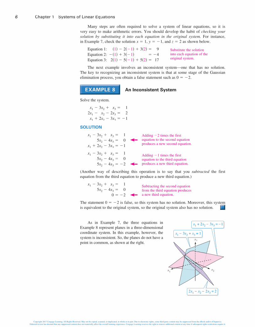
The next example involves an inconsistent system—one that has no solution. The key to recognizing an inconsistent system is that at some stage of the Gaussian elimination process, you obtain a false statement such as 0 = −2.
an Inconsistent System
Solve the system.
x1 −2x1 −x1 +
3x2 +x2 −
2x2 −
x3 =2x3 =3x3 =
12
−1
SoLutIon
x1 − 3x2 +5x2 −
x1 + 2x2 −
x3 =4x3 =3x3 =
10
−1
Adding −2 times the first equation to the second equation produces a new second equation.
x1 − 3x2 +5x2 −5x2 −
x3 =4x3 =4x3 =
10
−2
Adding −1 times the first equation to the third equation produces a new third equation.
(Another way of describing this operation is to say that you subtracted the first equation from the third equation to produce a new third equation.)
x1 − 3x2 +5x2 −
x3 =4x3 =
0 =
10
−2
Subtracting the second equation from the third equation produces a new third equation.
The statement 0 = −2 is false, so this system has no solution. Moreover, this system is equivalent to the original system, so the original system also has no solution.
As in Example 7, the three equations in Example 8 represent planes in a three-dimensional coordinate system. In this example, however, the system is inconsistent. So, the planes do not have a point in common, as shown at the right.
x2x1
x3
2x1 − x2 − 2x3 = 2
x1 + 2x2 − 3x3 = −1
x1 − 3x2 + x3 = 1
Copyright 2017 Cengage Learning. All Rights Reserved. May not be copied, scanned, or duplicated, in whole or in part. Due to electronic rights, some third party content may be suppressed from the eBook and/or eChapter(s). Editorial review has deemed that any suppressed content does not materially affect the overall learning experience. Cengage Learning reserves the right to remove additional content at any time if subsequent rights restrictions require it.
https://www.book4me.xyz/elementary-linear-algebra-larson/

1.1 Introduction to Systems of Linear Equations 9
This section ends with an example of a system of linear equations that has infinitely many solutions. You can represent the solution set for such a system in parametric form, as you did in Examples 2 and 3.
a System with Infinitely many Solutions
Solve the system.
x1
−x1
x2
+ 3x2
−−
x3 =3x3 =
=
0−1
1
SoLutIon
Begin by rewriting the system in row-echelon form, as shown below.
x1
−x1
x2
+ 3x2
−−
3x3 =x3 =
=
−101
Interchange the first two equations.
x1 −x2 −
3x2 −
3x3 =x3 =
3x3 =
−100
Adding the first equation to the third equation produces a new third equation.
x1 − x2 −
3x3 =x3 =0 =
−100
Adding −3 times the second equation to the third equation eliminates the third equation.
The third equation is unnecessary, so omit it to obtain the system shown below.
x1 − x2 −
3x3 =x3 =
−10
To represent the solutions, choose x3 to be the free variable and represent it by the parameter t. Because x2 = x3 and x1 = 3x3 − 1, you can describe the solution set as
x1 = 3t − 1, x2 = t, x3 = t, t is any real number.
DISCOVERY 1. Graph the two lines represented by the system of equations.
x − 2y =
−2x + 3y =1
−3
2. Use Gaussian elimination to solve this system as shown below.
x − 2y =
−1y =1
−1
x − 2y = 1
y = 1
x = 3y = 1
Graph the system of equations you obtain at each step of this process. What do you observe about the lines?
See LarsonLinearAlgebra.com for an interactive version of this type of exercise.
rEmarKYou are asked to repeat this graphical analysis for other systems in Exercises 91 and 92.
Copyright 2017 Cengage Learning. All Rights Reserved. May not be copied, scanned, or duplicated, in whole or in part. Due to electronic rights, some third party content may be suppressed from the eBook and/or eChapter(s). Editorial review has deemed that any suppressed content does not materially affect the overall learning experience. Cengage Learning reserves the right to remove additional content at any time if subsequent rights restrictions require it.
https://www.book4me.xyz/elementary-linear-algebra-larson/

10 Chapter 1 Systems of Linear Equations
1.1 Exercises See CalcChat.com for worked-out solutions to odd-numbered exercises.
Linear Equations In Exercises 1–6, determine whether the equation is linear in the variables x and y.
1. 2x − 3y = 4 2. 3x − 4xy = 0
3. 3y
+2x
− 1 = 0 4. x2 + y2 = 4
5. 2 sin x − y = 14 6. (cos 3)x + y = −16
Parametric representation In Exercises 7–10, find a parametric representation of the solution set of the linear equation.
7. 2x − 4y = 0 8. 3x − 12y = 9
9. x + y + z = 1
10. 12x1 + 24x2 − 36x3 = 12
graphical analysis In Exercises 11–24, graph the system of linear equations. Solve the system and interpret your answer.
11. 2x + y = 4x − y = 2
12.
x + 3y = 2
−x + 2y = 3
13. −x +3x −
y = 13y = 4
14.
12x − 1
3y =−2x + 4
3y =1
−4
15. 3x −2x +
5y = 7y = 9
16.
−x + 3y =4x + 3y =
177
17. 2x − y =5x − y =
511
18.
x − 5y = 21
6x + 5y = 21
19.
x + 34
+y − 1
3=
2x − y =
1
12
20.
x − 12
+y + 2
3= 4
x − 2y = 5
21. 0.05x − 0.03y = 0.070.07x + 0.02y = 0.16
22.
0.2x − 0.5y =0.3x − 0.4y =
−27.868.7
23.
x4
+y6
= 1
x − y = 3
24.
2x3
+
4x +
y6
=
y =
234
back-Substitution In Exercises 25–30, use back‑ substitution to solve the system.
25.
x1 − x2 = 2x2 = 3
26.
2x1 − 4x2 = 6
3x2 = 9
27. −x + y −
2y +z =z =
12z =
030
28.
x − y3y +
=z =
4z =
5118
29. 5x1 +2x1 +
2x2
x2
+ x3 = 0= 0
30.
x1 + x2
x2
+ x3 = 0= 0
graphical analysis In Exercises 31–36, complete parts (a)–(e) for the system of equations.
(a) Use a graphing utility to graph the system.
(b) Use the graph to determine whether the system is consistent or inconsistent.
(c) If the system is consistent, approximate the solution.
(d) Solve the system algebraically.
(e) Compare the solution in part (d) with the approximation in part (c). What can you conclude?
31.
−3x −6x +
y = 32y = 1
32.
4x −
−8x +5y =
10y =3
14
33. 2x −12x +
8y = 3y = 0
34.
9x −12x +
4y = 513y = 0
35.
4x −0.8x −
8y =1.6y =
91.8
36.
−14.7x +
44.1x −2.1y =6.3y =
1.05−3.15
System of Linear Equations In Exercises 37–56, solve the system of linear equations.
37.
x1 −3x1 −
x2 =2x2 =
0−1
38.
3x + 2y =6x + 4y =
214
39. 3u +u +
v = 2403v = 240
40.
x1 − 2x2 = 0
6x1 + 2x2 = 0
41. 9x − 3y = −1
15x + 2
5y = −13
42.
23x1 +4x1 +
16x2 = 0x2 = 0
43.
x − 24
+y − 1
3=
x − 3y =
2
20
44.
x1 + 43
+x2 + 1
2=
3x1 − x2 =
1
−2
45. 0.02x1 − 0.05x2 =0.03x1 + 0.04x2 =
−0.190.52
46. 0.05x1 − 0.03x2 = 0.210.07x1 + 0.02x2 = 0.17
47.
xx
2x
−+
y2y
− z = 0− z = 6− z = 5
48.
x +−x +4x +
y3yy
++
z = 22z = 8
= 4
49. 3x1 −x1 +
2x1 −
2x2 +x2 −
3x2 +
4x3 = 12x3 = 36x3 = 8
The symbol indicates an exercise in which you are instructed to use a graphing utility or software program.
Copyright 2017 Cengage Learning. All Rights Reserved. May not be copied, scanned, or duplicated, in whole or in part. Due to electronic rights, some third party content may be suppressed from the eBook and/or eChapter(s). Editorial review has deemed that any suppressed content does not materially affect the overall learning experience. Cengage Learning reserves the right to remove additional content at any time if subsequent rights restrictions require it.
https://www.book4me.xyz/elementary-linear-algebra-larson/

1.1 Exercises 11
50. 5x1 −2x1 +x1 −
3x2 +4x2 −
11x2 +
2x3 = 3x3 = 7
4x3 = 3
51.
2x1
4x1
−2x1
+
+
x2 −+
3x2 −
3x3 =2x3 =
13x3 =
410
−8
52.
x1
4x1
2x1
− 2x2
− 2x2
++−
4x3 =x3 =
7x3 =
137
−19
53.
x −5x −
3y +15y +
2z = 1810z = 18
54.
x1 − 2x2 +3x1 + 2x2 −
5x3 =x3 =
2−2
55.
x +2x +
−3x +x +
y3y4y2y
+ z
+ z− z
+−++
w = 6w = 0
2w = 4w = 0
56.
−x1
3x1 −
4x2
x2
2x2
−
+
x3
3x3
+−−
2x4 = 1x4 = 2x4 = 0
= 4
System of Linear Equations In Exercises 57–62, use a software program or a graphing utility to solve the system of linear equations.
57. 123.5x + 61.3y − 32.4z =54.7x − 45.6y + 98.2z =42.4x − 89.3y + 12.9z =
−262.74197.4 33.66
58. 120.2x + 62.4y − 36.5z =56.8x − 42.8y + 27.3z =88.1x + 72.5y − 28.5z =
258.64−71.44225.88
59.
x1 +0.5x1 +
0.33x1 +0.25x1 +
0.5x2 +0.33x2 +0.25x2 +0.2x2 +
0.33x3 +0.25x3 +0.2x3 +
0.17x3 +
0.25x4 = 1.10.21x4 = 1.20.17x4 = 1.30.14x4 = 1.4
60.
0.1x − 2.5y + 1.2z −2.4x + 1.5y − 1.8z +0.4x − 3.2y + 1.6z −1.6x + 1.2y − 3.2z +
0.75w =0.25w =1.4w =0.6w =
108−81148
−143.8.2
61.
12x1 − 3
7x2 + 29x3 =
23x1 + 4
9x2 − 25x3 =
45x1 − 1
8x2 + 43x3 =
349630
−1945
139150
62. 18x − 1
7y + 16z − 1
5w = 1
17x + 1
6y − 15z + 1
4w = 1
16x − 1
5y + 14z − 1
3w = 1
15x + 1
4y − 13z + 1
2w = 1
number of Solutions In Exercises 63–66, state why the system of equations must have at least one solution. Then solve the system and determine whether it has exactly one solution or infinitely many solutions.
63. 4x + 3y + 17z = 05x + 4y + 22z = 04x + 2y + 19z = 0
64.
2x + 3y4x + 3y8x + 3y
−+
= 0z = 0
3z = 0
65.
5x +10x +5x +
5y −5y +
15y −
z = 02z = 09z = 0
66. 16x + 3y + z = 0
16x + 2y − z = 0
67. nutrition One eight-ounce glass of apple juice and one eight-ounce glass of orange juice contain a total of 227 milligrams of vitamin C. Two eight-ounce glasses of apple juice and three eight-ounce glasses of orange juice contain a total of 578 milligrams of vitamin C. How much vitamin C is in an eight-ounce glass of each type of juice?
68. airplane Speed Two planes start from Los Angeles International Airport and fly in opposite directions. The second plane starts 1
2 hour after the first plane, but its speed is 80 kilometers per hour faster. Two hours after the first plane departs, the planes are 3200 kilometers apart. Find the airspeed of each plane.
true or False? In Exercises 69 and 70, determine whether each statement is true or false. If a statement is true, give a reason or cite an appropriate statement from the text. If a statement is false, provide an example that shows the statement is not true in all cases or cite an appropriate statement from the text.
69. (a) A system of one linear equation in two variables is always consistent.
(b) A system of two linear equations in three variables is always consistent.
(c) If a linear system is consistent, then it has infinitely many solutions.
70. (a) A linear system can have exactly two solutions.
(b) Two systems of linear equations are equivalent when they have the same solution set.
(c) A system of three linear equations in two variables is always inconsistent.
71. Find a system of two equations in two variables, x1 and x2, that has the solution set given by the parametric representation x1 = t and x2 = 3t − 4, where t is any real number. Then show that the solutions to the system can also be written as
x1 =43
+t3
and x2 = t.
The symbol indicates that electronic data sets for these exercises are available at LarsonLinearAlgebra.com. The data sets are compatible with MATLAB, Mathematica, Maple, TI-83 Plus, TI-84 Plus, TI-89, and Voyage 200.
Copyright 2017 Cengage Learning. All Rights Reserved. May not be copied, scanned, or duplicated, in whole or in part. Due to electronic rights, some third party content may be suppressed from the eBook and/or eChapter(s). Editorial review has deemed that any suppressed content does not materially affect the overall learning experience. Cengage Learning reserves the right to remove additional content at any time if subsequent rights restrictions require it.
https://www.book4me.xyz/elementary-linear-algebra-larson/

12 Chapter 1 Systems of Linear Equations
72. Find a system of two equations in three variables, x1, x2, and x3, that has the solution set given by the parametric representation
x1 = t, x2 = s, and x3 = 3 + s − t
where s and t are any real numbers. Then show that the solutions to the system can also be written as
x1 = 3 + s − t, x2 = s, and x3 = t.
Substitution In Exercises 73–76, solve the system of equations by first letting A = 1�x, B = 1�y, and C = 1�z.
73.
12x
−12y
= 7
3x
+4y
= 0
74.
3x
+2y
=
2x
−3y
=
−1
−176
75.
2x4x
−2x
+1y
+3y
−3z
=
+2z
=
−13z
=
4
10
−8
76.
2x
+1y
3x
−4y
2x
+1y
−2z
=
=
+3z
=
5
−1
0
trigonometric Coefficients In Exercises 77 and 78, solve the system of linear equations for x and y.
77. (cos θ)x + (sin θ)y = 1 (−sin θ)x + (cos θ)y = 0
78. (cos θ)x + (sin θ)y = 1 (−sin θ)x + (cos θ)y = 1
Coefficient Design In Exercises 79–84, determine the value(s) of k such that the sys tem of linear equations has the indicated number of solutions.
79. No solution 80. Exactly one solution
x +
kx +ky = 2y = 4
x +
kx +ky = 0y = 0
81. Exactly one solution 82. No solution
kx +x +
2x −
2ky +y +y +
3kz =z =z =
4k01
x + 2y + kz = 6
3x + 6y + 8z = 4
83. Infinitely many solutions
4x +kx +
ky =y =
6−3
84. Infinitely many solutions
kx +3x −
y =4y =
16−64
85. Determine the values of k such that the system of linear equations does not have a unique solution.
x +x +
kx +
y +ky +y +
kz = 3z = 2z = 1
86. CAPSTONE Find values of a, b, and c such that the system of linear equations has (a) exactly one solution, (b) infinitely many solutions, and (c) no solution. Explain.
x + 5y +x + 6y −
2x + ay +
z = 0z = 0
bz = c
87. Writing Consider the system of linear equations in x and y.
a1x + b1y = c1
a2x + b2y = c2
a3x + b3y = c3
Describe the graphs of these three equations in the xy-plane when the system has (a) exactly one solution, (b) infinitely many solutions, and (c) no solution.
88. Writing Explain why the system of linear equations in Exercise 87 must be consistent when the constant terms c1, c2, and c3 are all zero.
89. Show that if ax2 + bx + c = 0 for all x, then a = b = c = 0.
90. Consider the system of linear equations in x and y.
ax +cx +
by =dy =
ef
Under what conditions will the system have exactly one solution?
Discovery In Exercises 91 and 92, sketch the lines represented by the system of equations. Then use Gaussian elimination to solve the system. At each step of the elimination process, sketch the corresponding lines. What do you observe about the lines?
91.
x − 4y =5x − 6y =
−313
92.
2x −
−4x +3y =6y =
7−14
Writing In Exercises 93 and 94, the graphs of the two equations appear to be parallel. Solve the system of equations algebraically. Explain why the graphs are misleading.
93. 100y − x =99y − x =
200−198
94.
21x − 20y =13x − 12y =
0120
−1−3 1 2 3 4
−3−4
1
34
y
x
−10 10 20
10
20
y
x
Copyright 2017 Cengage Learning. All Rights Reserved. May not be copied, scanned, or duplicated, in whole or in part. Due to electronic rights, some third party content may be suppressed from the eBook and/or eChapter(s). Editorial review has deemed that any suppressed content does not materially affect the overall learning experience. Cengage Learning reserves the right to remove additional content at any time if subsequent rights restrictions require it.
https://www.book4me.xyz/elementary-linear-algebra-larson/

1.2 Gaussian Elimination and Gauss-Jordan Elimination 13
1.2 Gaussian Elimination and Gauss-Jordan Elimination
Determine the size of a matrix and write an augmented or coefficient matrix from a system of linear equations.
Use matrices and Gaussian elimination with back-substitution to solve a system of linear equations.
Use matrices and Gauss-Jordan elimination to solve a system of linear equations.
Solve a homogeneous system of linear equations.
MatricEs
Section 1.1 introduced Gaussian elimination as a procedure for solving a system of linear equations. In this section, you will study this procedure more thoroughly, beginning with some definitions. The first is the definition of a matrix.
The entry aij is located in the ith row and the jth column. The index i is called the row subscript because it identifies the row in which the entry lies, and the index j is called the column subscript because it identifies the column in which the entry lies.
A matrix with m rows and n columns is of size m × n. When m = n, the matrix is square of order n and the entries a11, a22, a33, . . . , ann are the main diagonal entries.
sizes of Matrices
Each matrix has the indicated size.
a. [2] Size: 1 × 1 b. [00
00] Size: 2 × 2 c. [ e
π2
√2−7
4] Size: 2 × 3
One common use of matrices is to represent systems of linear equations. The matrix derived from the coefficients and constant terms of a system of linear equations is the augmented matrix of the system. The matrix containing only the coefficients of the system is the coefficient matrix of the system. Here is an example.
System Augmented Matrix Cofficient Matrix
x−x2x
− 4y+ 3y
+−−
3z =z =
4z =
5−3
6 [
1−1
2
−430
3−1−4
5−3
6] [1
−12
−430
3−1−4]
Definition of a Matrix
If m and n are positive integers, then an m × n (read “m by n”) matrix is a rectangular array
Column 1 Column 2 Column 3 . . . Column n
Row 1
Row 2
Row 3
⋮Row m
[
a11
a21
a31
⋮am1
a12
a22
a32
⋮am2
a13
a23
a33
⋮am3
. . .
. . .
. . .
. . .
a1n
a2n
a3n
⋮amn
]in which each entry, aij, of the matrix is a number. An m × n matrix has m rows and n columns. Matrices are usually denoted by capital letters.
rEMarKThe plural of matrix is matrices. When each entry of a matrix is a real number, the matrix is a real matrix. Unless stated otherwise, assume all matrices in this text are real matrices.
rEMarKBegin by aligning the variables in the equations vertically. Use 0 to show coefficients of zero in the matrix. Note the fourth column of constant terms in the augmented matrix.
Copyright 2017 Cengage Learning. All Rights Reserved. May not be copied, scanned, or duplicated, in whole or in part. Due to electronic rights, some third party content may be suppressed from the eBook and/or eChapter(s). Editorial review has deemed that any suppressed content does not materially affect the overall learning experience. Cengage Learning reserves the right to remove additional content at any time if subsequent rights restrictions require it.
https://www.book4me.xyz/elementary-linear-algebra-larson/
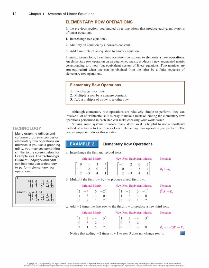
14 Chapter 1 Systems of Linear Equations
ElEMEntary row opErations
In the previous section, you studied three operations that produce equivalent systems of linear equations.
1. Interchange two equations.
2. Multiply an equation by a nonzero constant.
3. Add a multiple of an equation to another equation.
In matrix terminology, these three operations correspond to elementary row operations. An elementary row operation on an augmented matrix produces a new augmented matrix corresponding to a new (but equivalent) system of linear equations. Two matrices are row-equivalent when one can be obtained from the other by a finite sequence of elementary row operations.
Although elementary row operations are relatively simple to perform, they can involve a lot of arithmetic, so it is easy to make a mistake. Noting the elementary row operations performed in each step can make checking your work easier.
Solving some systems involves many steps, so it is helpful to use a shorthand method of notation to keep track of each elementary row operation you perform. The next example introduces this notation.
Elementary row operations
a. Interchange the first and second rows.
Original Matrix New Row-Equivalent Matrix Notation
[0
−12
12
−3
304
431] [
−102
21
−3
034
341] R1↔ R2
b. Multiply the first row by 12 to produce a new first row.
Original Matrix New Row-Equivalent Matrix Notation
[215
−43
−2
6−3
1
−202] [
115
−23
−2
3−3
1
−102]
(12)R1→ R1
c. Add −2 times the first row to the third row to produce a new third row.
Original Matrix New Row-Equivalent Matrix Notation
[102
231
−4−2
5
3−1−2] [
100
23
−3
−4−213
3−1−8]
R3 + (−2)R1 → R3
Notice that adding −2 times row 1 to row 3 does not change row 1.
Elementary row operations
1. Interchange two rows.2. Multiply a row by a nonzero constant.3. Add a multiple of a row to another row.
tEchnoloGyMany graphing utilities and software programs can perform elementary row operations on matrices. If you use a graphing utility, you may see something similar to the screen below for Example 2(c). The technology Guide at CengageBrain.com can help you use technology to perform elementary row operations.
mRAdd(-2,A,1,3) [[1 2 -4 3 ][0 3 -2 -1][0 -3 13 -8]]
[[1 2 -4 3 ][0 3 -2 -1][2 1 5 -2]]
A
Copyright 2017 Cengage Learning. All Rights Reserved. May not be copied, scanned, or duplicated, in whole or in part. Due to electronic rights, some third party content may be suppressed from the eBook and/or eChapter(s). Editorial review has deemed that any suppressed content does not materially affect the overall learning experience. Cengage Learning reserves the right to remove additional content at any time if subsequent rights restrictions require it.
https://www.book4me.xyz/elementary-linear-algebra-larson/

1.2 Gaussian Elimination and Gauss-Jordan Elimination 15
In Example 7 in Section 1.1, you used Gaussian elimination with back-substitution to solve a system of linear equations. The next example demonstrates the matrix version of Gaussian elimination. The two methods are essentially the same. The basic difference is that with matrices you do not need to keep writing the variables.
Using Elementary row operations to solve a system
Linear System Associated Augmented Matrix
x − 2y−x + 3y2x − 5y
+ 3z ==
+ 5z =
9−417
[1
−12
−23
−5
305
9−417]
Add the first equation to the second Add the first row to the second row to equation. produce a new second row.
x − 2y + 3z =y + 3z =
2x − 5y + 5z =
95
17 [
102
−21
−5
335
95
17] R2 + R1 → R2
Add −2 times the first equation to the Add −2 times the first row to the third third equation. row to produce a new third row.
x − 2y +y +
−y −
3z =3z =z =
95
−1 [
100
−21
−1
33
−1
95
−1] R3 + (−2)R1 → R3
Add the second equation to the third Add the second row to the third row toequation. produce a new third row.
x − 2y + 3z = 9y + 3z = 5
2z = 4 [
100
−210
332
954]
R3 + R2 → R3
Multiply the third equation by 12. Multiply the third row by 12 to produce a new third row.
x − 2y + 3z = 9y + 3z = 5
z = 2 [
100
−210
331
952]
(12)R3 → R3
Use back-substitution to find the solution, as in Example 6 in Section 1.1. The solution is x = 1, y = −1, and z = 2.
The last matrix in Example 3 is in row-echelon form. To be in this form, a matrix must have the properties listed below.
row-Echelon Form and reduced row-Echelon Form
A matrix in row-echelon form has the properties below.
1. Any rows consisting entirely of zeros occur at the bottom of the matrix.2. For each row that does not consist entirely of zeros, the first nonzero entry
is 1 (called a leading 1).3. For two successive (nonzero) rows, the leading 1 in the higher row is farther
to the left than the leading 1 in the lower row.
A matrix in row-echelon form is in reduced row-echelon form when every column that has a leading 1 has zeros in every position above and below its leading 1.
rEMarKThe term echelon refers to the stair-step pattern formed by the nonzero elements of the matrix.
Copyright 2017 Cengage Learning. All Rights Reserved. May not be copied, scanned, or duplicated, in whole or in part. Due to electronic rights, some third party content may be suppressed from the eBook and/or eChapter(s). Editorial review has deemed that any suppressed content does not materially affect the overall learning experience. Cengage Learning reserves the right to remove additional content at any time if subsequent rights restrictions require it.
https://www.book4me.xyz/elementary-linear-algebra-larson/

16 Chapter 1 Systems of Linear Equations
row-Echelon Form
Determine whether each matrix is in row-echelon form. If it is, determine whether the matrix is also in reduced row-echelon form.
a. [100
210
−101
43
−2] b. [100
201
−102
20
−4]c. [
1000
−5000
2100
−1310
3−2
41] d. [
1000
0100
0010
−1230]
e. [100
220
−311
4−1−3] f. [
000
100
010
530]
solUtion
The matrices in (a), (c), (d), and (f) are in row-echelon form. The matrices in (d) and (f) are in reduced row-echelon form because every column that has a leading 1 has zeros in every position above and below its leading 1. The matrix in (b) is not in row-echelon form because the row of all zeros does not occur at the bottom of the matrix. The matrix in (e) is not in row-echelon form because the first nonzero entry in Row 2 is not 1.
Every matrix is row-equivalent to a matrix in row-echelon form. For instance, in Example 4(e), multiplying the second row in the matrix by 1
2 changes the matrix to row-echelon form.
The procedure for using Gaussian elimination with back-substitution is summarized below.
Gaussian elimination with back-substitution works well for solving systems of linear equations by hand or with a computer. For this algorithm, the order in which you perform the elementary row operations is important. Operate from left to right by columns, using elementary row operations to obtain zeros in all entries directly below the leading 1’s.
Gaussian Elimination with Back-substitution
1. Write the augmented matrix of the system of linear equations.2. Use elementary row operations to rewrite the matrix in row-echelon form.3. Write the system of linear equations corresponding to the matrix in
row-echelon form, and use back-substitution to find the solution.
tEchnoloGyUse a graphing utility or a software program to find the row-echelon forms of the matrices in Examples 4(b) and 4(e) and the reduced row-echelon forms of the matrices in Examples 4(a), 4(b), 4(c), and 4(e). The technology Guide at CengageBrain.com can help you use technology to find the row-echelon and reduced row-echelon forms of a matrix. Similar exercises and projects are also available on the website.
edobric/Shutterstock.com
linEaralGEBraappliED
The Global Positioning System (GPS) is a network of 24 satellites originally developed by the U.S. military as a navigational tool. Today, GPS technology is used in a wide variety of civilian applications, such as package delivery, farming, mining, surveying, construction, banking, weather forecasting, and disaster relief. A GPS receiver works by using satellite readings to calculate its location. In three dimensions, the receiver uses signals from at least four satellites to “trilaterate” its position. In a simplified mathematical model, a system of three linear equations in four unknowns (three dimensions and time) is used to determine the coordinates of the receiver as functions of time.
Copyright 2017 Cengage Learning. All Rights Reserved. May not be copied, scanned, or duplicated, in whole or in part. Due to electronic rights, some third party content may be suppressed from the eBook and/or eChapter(s). Editorial review has deemed that any suppressed content does not materially affect the overall learning experience. Cengage Learning reserves the right to remove additional content at any time if subsequent rights restrictions require it.
https://www.book4me.xyz/elementary-linear-algebra-larson/

1.2 Gaussian Elimination and Gauss-Jordan Elimination 17
Gaussian Elimination with Back-substitution
Solve the system.
x1 +2x1 +x1 −
x2 +2x2 −4x2 +4x2 −
x3
x3
x3
7x3
−
−−
2x4 ==
3x4 =x4 =
−32
−2−19
solUtion
The augmented matrix for this system is
[0121
124
−4
1−1
1−7
−20
−3−1
−32
−2−19
].
Obtain a leading 1 in the upper left corner and zeros elsewhere in the first column.
[1021
214
−4
−111
−7
0−2−3−1
2−3−2
−19]
Interchange the first two rows.
R1 ↔ R2
[1001
210
−4
−113
−7
0−2−3−1
2−3−6
−19]
Adding −2 times the first row to the third row produces a new third row.
R3 + (−2)R1 → R3
[1000
210
−6
−113
−6
0−2−3−1
2−3−6
−21]
Adding −1 times the first row to the fourth row produces a new fourth row.
R4 + (−1)R1 → R4
Now that the first column is in the desired form, change the second column as shown below.
[1000
2100
−1130
0−2−3
−13
2−3−6
−39]
Adding 6 times the second row to the fourth row produces a new fourth row.
R4 + (6)R2 → R4
To write the third and fourth columns in proper form, multiply the third row by 13 and the fourth row by − 1
13.
[1000
2100
−1110
0−2−1
1
2−3−2
3]
Multiplying the third row by 13 and the fourth row by − 1
13 produces new third and fourth rows.
(13)R3 → R3
(− 113)R4 → R4
The matrix is now in row-echelon form, and the corresponding system is shown below.
x1 + 2x2 − x3
x2 + x3
x3
−−
=2x4 =x4 =x4 =
2−3−2
3
Use back-substitution to find that the solution is x1 = −1, x2 = 2, x3 = 1, and x4 = 3.
Copyright 2017 Cengage Learning. All Rights Reserved. May not be copied, scanned, or duplicated, in whole or in part. Due to electronic rights, some third party content may be suppressed from the eBook and/or eChapter(s). Editorial review has deemed that any suppressed content does not materially affect the overall learning experience. Cengage Learning reserves the right to remove additional content at any time if subsequent rights restrictions require it.
https://www.book4me.xyz/elementary-linear-algebra-larson/
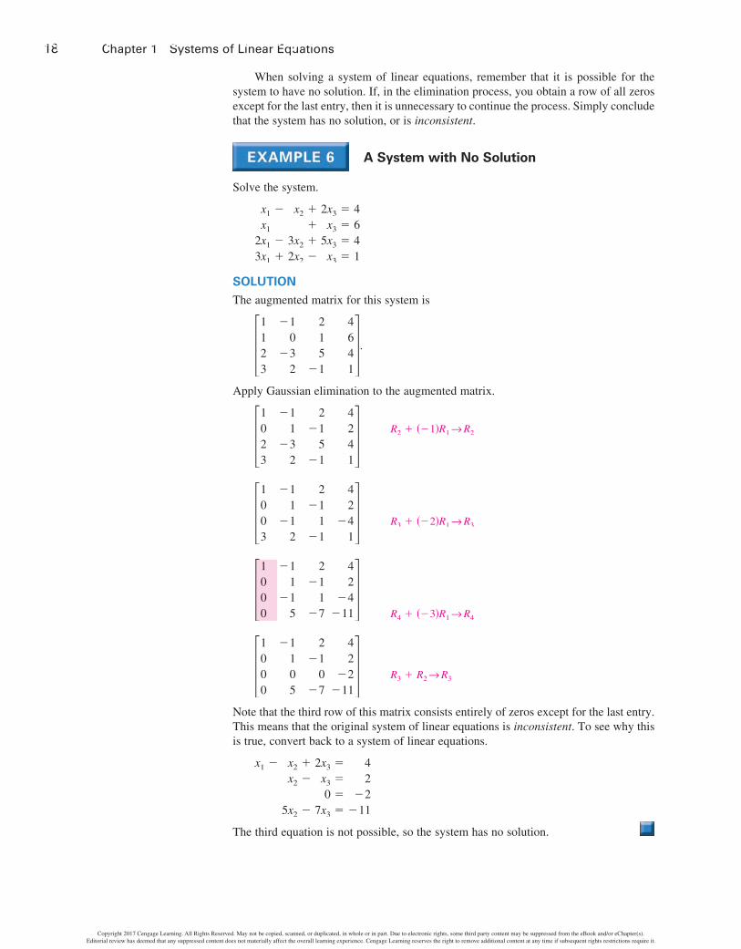
18 Chapter 1 Systems of Linear Equations
When solving a system of linear equations, remember that it is possible for the system to have no solution. If, in the elimination process, you obtain a row of all zeros except for the last entry, then it is unnecessary to continue the process. Simply conclude that the system has no solution, or is inconsistent.
a system with no solution
Solve the system.
x1
x1
2x1
3x1
−
−+
x2 ++
3x2 +2x2 −
2x3 = 4x3 = 6
5x3 = 4x3 = 1
solUtion
The augmented matrix for this system is
[1123
−10
−32
215
−1
4641].
Apply Gaussian elimination to the augmented matrix.
[1023
−11
−32
2−1
5−1
4241]
R2 + (−1)R1 → R2
[1003
−11
−12
2−1
1−1
42
−41]
R3 + (−2)R1 → R3
[1000
−11
−15
2−1
1−7
42
−4−11
]
R4 + (−3)R1 → R4
[1000
−1105
2−1
0−7
42
−2−11
] R3 + R2 → R3
Note that the third row of this matrix consists entirely of zeros except for the last entry. This means that the original system of linear equations is inconsistent. To see why this is true, convert back to a system of linear equations.
x1 − x2 +x2 −
5x2 −
2x3 =x3 =0 =
7x3 =
42
−2−11
The third equation is not possible, so the system has no solution.
Copyright 2017 Cengage Learning. All Rights Reserved. May not be copied, scanned, or duplicated, in whole or in part. Due to electronic rights, some third party content may be suppressed from the eBook and/or eChapter(s). Editorial review has deemed that any suppressed content does not materially affect the overall learning experience. Cengage Learning reserves the right to remove additional content at any time if subsequent rights restrictions require it.
https://www.book4me.xyz/elementary-linear-algebra-larson/
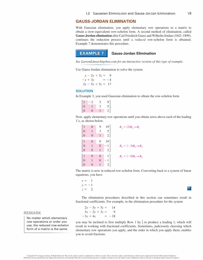
1.2 Gaussian Elimination and Gauss-Jordan Elimination 19
GaUss-JorDan EliMination
With Gaussian elimination, you apply elementary row operations to a matrix to obtain a (row-equivalent) row-echelon form. A second method of elimination, called Gauss-Jordan elimination after Carl Friedrich Gauss and Wilhelm Jordan (1842–1899),continues the reduction process until a reduced row-echelon form is obtained. Example 7 demonstrates this procedure.
Gauss-Jordan Elimination
See LarsonLinearAlgebra.com for an interactive version of this type of example.
Use Gauss-Jordan elimination to solve the system.
x − 2y−x + 3y2x − 5y
+ 3z ==
+ 5z =
9−417
solUtion
In Example 3, you used Gaussian elimination to obtain the row-echelon form
[100
−210
331
952].
Now, apply elementary row operations until you obtain zeros above each of the leading 1’s, as shown below.
[100
010
931
1952]
R1 + (2)R2 → R1
[100
010
901
19−1
2] R2 + (−3)R3 → R2
[100
010
001
1−1
2] R1 + (−9)R3 → R1
The matrix is now in reduced row-echelon form. Converting back to a system of linear equations, you have
x =y =z =
1−1
2.
The elimination procedures described in this section can sometimes result in fractional coefficients. For example, in the elimination procedure for the system
2x − 5y3x − 2y
−3x + 4y
+ 5z =+ 3z =
=
149
−18
you may be inclined to first multiply Row 1 by 12 to produce a leading 1, which will
result in working with fractional coefficients. Sometimes, judiciously choosing which elementary row operations you apply, and the order in which you apply them, enables you to avoid fractions.
rEMarKNo matter which elementary row operations or order you use, the reduced row-echelon form of a matrix is the same.
Copyright 2017 Cengage Learning. All Rights Reserved. May not be copied, scanned, or duplicated, in whole or in part. Due to electronic rights, some third party content may be suppressed from the eBook and/or eChapter(s). Editorial review has deemed that any suppressed content does not materially affect the overall learning experience. Cengage Learning reserves the right to remove additional content at any time if subsequent rights restrictions require it.
https://www.book4me.xyz/elementary-linear-algebra-larson/

20 Chapter 1 Systems of Linear Equations
The next example demonstrates how Gauss-Jordan elimination can be used to solve a system with infinitely many solutions.
a system with infinitely Many solutions
Solve the system of linear equations.
2x1 + 4x2
3x1 + 5x2
− 2x3 = 0= 1
solUtion
The augmented matrix for this system is
[23
45
−20
01].
Using a graphing utility, a software program, or Gauss-Jordan elimination, verify that the reduced row-echelon form of the matrix is
[10
01
5−3
2−1].
The corresponding system of equations is
x1 + 5x3 =x2 − 3x3 =
2−1.
Now, using the parameter t to represent x3, you have
x1 = 2 − 5t, x2 = −1 + 3t, x3 = t, t is any real number.
Note in Example 8 that the arbitrary parameter t represents the nonleading variable x3. The variables x1 and x2 are written as functions of t.
You have looked at two elimination methods for solving a system of linear equations. Which is better? To some degree the answer depends on personal preference. In real-life applications of linear algebra, systems of linear equations are usually solved by computer. Most software uses a form of Gaussian elimination, with special emphasis on ways to reduce rounding errors and minimize storage of data. The examples and exercises in this text focus on the underlying concepts, so you should know both elimination methods.
DISCOVERY 1. Without performing any row operations, explain why the system of
linear equations below is consistent.
2x1 + 3x2 +−5x1 + 6x2 −
7x1 − 4x2 +
5x3 = 017x3 = 03x3 = 0
2. The system below has more variables than equations. Why does it have an infinite number of solutions?
2x1 + 3x2 +−5x1 + 6x2 −
7x1 − 4x2 +
5x3 +17x3 −3x3 +
2x4 = 03x4 = 0
13x4 = 0
Copyright 2017 Cengage Learning. All Rights Reserved. May not be copied, scanned, or duplicated, in whole or in part. Due to electronic rights, some third party content may be suppressed from the eBook and/or eChapter(s). Editorial review has deemed that any suppressed content does not materially affect the overall learning experience. Cengage Learning reserves the right to remove additional content at any time if subsequent rights restrictions require it.
https://www.book4me.xyz/elementary-linear-algebra-larson/

1.2 Gaussian Elimination and Gauss-Jordan Elimination 21
hoMoGEnEoUs systEMs oF linEar EqUations
Systems of linear equations in which each of the constant terms is zero are called homogeneous. A homogeneous system of m equations in n variables has the form
a11x1 +a21x1 +
am1x1 +
a12x2 +a22x2 +
am2x2 +
a13x3 +a23x3 +
am3x3 +
. . . +
. . . +
. . . +
a1nxn = 0a2nxn = 0
⋮ amnxn = 0.
A homogeneous system must have at least one solution. Specifically, if all variables in a homogeneous system have the value zero, then each of the equations is satisfied. Such a solution is trivial (or obvious).
solving a homogeneous system of linear Equations
Solve the system of linear equations.
x1 − x2 + 3x3 = 02x1 + x2 + 3x3 = 0
solUtion
Applying Gauss-Jordan elimination to the augmented matrix
[12
−11
33
00]
yields the matrices shown below.
[10
−13
3−3
00]
R2 + (−2)R1 → R2
[10
−11
3−1
00] (1
3)R2 → R2
[10
01
2−1
00]
R1 + R2 → R1
The system of equations corresponding to this matrix is
x1 +x2 −
2x3 = 0x3 = 0.
Using the parameter t = x3, the solution set is x1 = −2t, x2 = t, and x3 = t, where t is any real number. This system has infinitely many solutions, one of which is the trivial solution (t = 0).
As illustrated in Example 9, a homogeneous system with fewer equations than variables has infinitely many solutions.
To prove Theorem 1.1, use the procedure in Example 9, but for a general matrix.
thEorEM 1.1 the number of solutions of a homogeneous system
Every homogeneous system of linear equations is consistent. Moreover, if the system has fewer equations than variables, then it must have infinitely many solutions.
rEMarKA homogeneous system of three equations in the three variables x1, x2, and x3 has the trivial solution x1 = 0, x2 = 0, and x3 = 0.
Copyright 2017 Cengage Learning. All Rights Reserved. May not be copied, scanned, or duplicated, in whole or in part. Due to electronic rights, some third party content may be suppressed from the eBook and/or eChapter(s). Editorial review has deemed that any suppressed content does not materially affect the overall learning experience. Cengage Learning reserves the right to remove additional content at any time if subsequent rights restrictions require it.
https://www.book4me.xyz/elementary-linear-algebra-larson/

22 Chapter 1 Systems of Linear Equations
1.2 Exercises See CalcChat.com for worked-out solutions to odd-numbered exercises.
Matrix size In Exercises 1–6, determine the size of the matrix.
1. [130
2−4
1
−462] 2. [
−2−1
12]
3. [ 2−6
−12
−10
11]
4. [−1]
5. [8211
611
−1
4−7−1
2
1420
3110]
6. [1 2 3 4 −10]
Elementary row operations In Exercises 7–10, identify the elementary row operation(s) being performed to obtain the new row-equivalent matrix. Original Matrix New Row-Equivalent Matrix
7. [−23
5−1
1−8] [13
30
−1 −39−8]
Original Matrix New Row-Equivalent Matrix
8. [ 3−4
−13
−47] [3
5−1
0−4−5]
Original Matrix New Row-Equivalent Matrix
9. [0
−13
−15
−2
−7−8
1
772] [
−100
5−113
−8−7
−23
77
23] Original Matrix New Row-Equivalent Matrix
10. [−1
25
−2−5
4
31
−7
−2−7
6] [−1
00
−2−9−6
378
−2−11−4]
augmented Matrix In Exercises 11–18, find the solution set of the system of linear equations represented by the augmented matrix.
11. [10
01
02] 12. [1
001
23]
13. [100
−110
0−2
1
31
−1] 14. [100
200
110
0−1
0]15. [
210
1−1
1
−112
301] 16. [
311
−120
111
502]
17. [1000
2100
0210
1121
4314]
18. [1000
2100
0310
1020
3102]
row-Echelon Form In Exercises 19–24, determine whether the matrix is in row-echelon form. If it is, determine whether it is also in reduced row-echelon form.
19. [100
010
010
020]
20. [01
10
02
01]
21. [−2
00
0−1
0
120
512]
22. [100
010
231
140]
23. [000
000
100
012
000]
24. [100
000
000
010]
system of linear Equations In Exercises 25–38, solve the system using ei ther Gaussian elimination with back-substitution or Gauss-Jordan elimination.
25.
x +3x +
3y =y =
119
26.
2x + 6y =−2x − 6y =
16−16
27. −x + 2y =2x − 4y =
13.5
28. 2x −3x +
y =2y =
−0.11.6
29. −3x + 5y =
3x + 4y =4x − 8y =
−224
32
30.
x +x +
3x −
2y = 0y = 6
2y = 8
Copyright 2017 Cengage Learning. All Rights Reserved. May not be copied, scanned, or duplicated, in whole or in part. Due to electronic rights, some third party content may be suppressed from the eBook and/or eChapter(s). Editorial review has deemed that any suppressed content does not materially affect the overall learning experience. Cengage Learning reserves the right to remove additional content at any time if subsequent rights restrictions require it.
https://www.book4me.xyz/elementary-linear-algebra-larson/