Field Scale Geomechanical Modelling Using a New Automated ...

2011 SIMULIA Customer Conference 1

Field Scale Geomechanical Modelling Using a New Automated Workflow in Abaqus

S. Monaco1, G. Capasso

1, D. Datye

2, S. Mantica

1 and R. Vitali

3

1. eni e&p, S. Donato Milanese (MI), Italy

2. Dassault Systèmes Simulia Corporation, Providence (RI), USA

3. Simulia Italia, Lainate (MI), Italy

Abstract: Abaqus has been used for many years in eni as the main stress/strain simulator for

studying the geomechanical behaviour of reservoirs both at field and well scale. In the work

presented in this paper, the new capabilities developed in Abaqus/CAE are applied with reference

to a field scale geomechanical study performed on a realistic test case. As shown in the example

application, the capabilities developed in Abaqus/CAE are particularly suitable for reservoir

geomechanical simulations, and allow one to perform accurate analyses that overcome the

limitations of the previous workflow and simultaneously provide significant automation.

Keywords: Cam-Clay, Constitutive Model, Faults, Geomechanics, Hydrocarbon Production,

Reservoir Compaction, Surface Subsidence.

1. Introduction

Up to now, the study of geomechanical effects due to field scale reservoir depletion has been

performed following the steps of the workflow developed internally by eni and described in

(Capasso and Mantica, 2006).

However, this workflow includes non-automated procedures as well as simplifications related to

the geometry description, such as smearing of faults and simplified treatment of collapsing layers.

The new features implemented in Abaqus 6.11 for soils analyses definitely change the approach to

geomechanical reservoir simulation by allowing a complete automated workflow that can be

managed through Abaqus/CAE.

A reservoir modeler plug-in, which covers all the steps of the standard workflow for subsidence

studies, has been implemented. Each task of the workflow from the creation of the Eclipse odb

using the translator (built in to establish a link between the flow-dynamic simulator Eclipse and

the stress simulator Abaqus) to the final step of computing the plastic properties is listed in the

GUI. The Upscaling and Burdens steps are performed outside of the plug-in, but their statuses are

documented within the plug-in and they are properly executed in Abaqus/CAE. All information

entered by the user is stored on the custom data base on a model-by-model basis and is persistent

across sessions. This allows for providing significant automation and makes it easier to the user to

complete all the steps for the creation of a reservoir model.

2 2011 SIMULIA Customer Conference

2. Overview of the methodology

2.1 Workflow overview

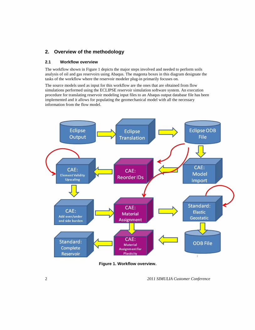
The workflow shown in Figure 1 depicts the major steps involved and needed to perform soils

analysis of oil and gas reservoirs using Abaqus. The magenta boxes in this diagram designate the

tasks of the workflow where the reservoir modeler plug-in primarily focuses on.

The source models used as input for this workflow are the ones that are obtained from flow

simulations performed using the ECLIPSE reservoir simulation software system. An execution

procedure for translating reservoir modeling input files to an Abaqus output database file has been

implemented and it allows for populating the geomechanical model with all the necessary

information from the flow model.

Figure 1. Workflow overview.


2.2 Reservoir Modeler Tree overview

A convenient, model tree-based approach is adopted for the Eclipse reservoir modeler GUI. A

new tab named “Reservoir Modeler” (RM) appears in the model tree when the plug-in is enabled;

this tab is in addition to the standard Abaqus/CAE model tree tabs Model and Results (and any

other custom tabs) as shown in Figure 2.

Figure 2. Expanded Tree of the Reservoir Modeler in Abaqus/CAE.

The creation of a model using the RM involves the completion of a sequence of steps which will

be described in detail in the next section. In order to perform any particular step, all of the

previous steps must have already been completed. The RM provides feedback on the progress of

each step by modifying the icons associated with each step. No icon indicates that the user has not

yet entered this information. A green check indicates that the user has entered this information and

any necessary tasks have been executed successfully. A red check indicates that the information

has been entered, but the step failed execution or is out-of-date due to changes to a previous step.

If changes are made to a given step, all the subsequent steps must then be regenerated.

This is the workflow and the GUI which have been adopted to perform the study of the synthetic

Brugge field. All the steps passed through to create the geomechanical model and to perform

elastic and elasto-plastic simulations are described in detail in the next section.


3. Reservoir geomechanical model generation workflow applied to the Brugge field

3.1 General description of the Brugge field

The Brugge field is a complete synthetic oil field whose structure consists of an E-W elongated

half-dome with a large boundary fault at its northern edge and one internal fault with a modest

throw.

The Eclipse model is composed of 139x48x9 cells in directions I, J and K respectively, adding up

to a total of 60048 cells among which 44464 are active. Figure 3 provides a top view of the first

reservoir layer where the intra-field fault is evident.

Figure 3. Brugge Field Eclipse discretization: top view of Layer 1.

The field has 10 injector and 20 producer wells, but for this study we consider the injectors to be

deactivated. The pressure controls on the bottom hole pressure has also been lowered in order to

obtain higher depletion and associated subsidence problems.

The production start is set for 1st March 2016 and the end on 1

st January 2028.

3.2 Eclipse output file translation

The first step in the creation of the reservoir model is performed by using the fromreservoir

translator to obtain an Abaqus output database (odb) file equivalent to the Eclipse model. The

Eclipse reservoir simulation data translation converts cell data to equivalent Abaqus element

definitions, and pressure history descriptions to pore pressure field output frames. The created odb


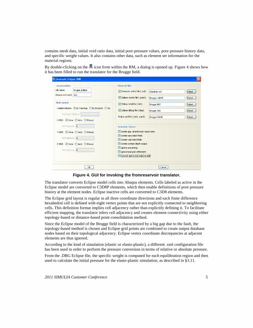
contains mesh data, initial void ratio data, initial pore pressure values, pore pressure history data,

and specific weight values. It also contains other data, such as element set information for the

material regions.

By double-clicking on the icon from within the RM, a dialog is opened up. Figure 4 shows how

it has been filled to run the translator for the Brugge field.

Figure 4. GUI for invoking the fromreservoir translator.

The translator converts Eclipse model cells into Abaqus elements. Cells labeled as active in the

Eclipse model are converted to C3D8P elements, which then enable definitions of pore pressure

history at the element nodes. Eclipse inactive cells are converted to C3D8 elements.

The Eclipse grid layout is regular in all three coordinate directions and each finite difference

hexahedral cell is defined with eight vertex points that are not explicitly connected to neighboring

cells. This definition format implies cell adjacency rather than explicitly defining it. To facilitate

efficient mapping, the translator infers cell adjacency and creates element connectivity using either

topology-based or distance-based point consolidation method.

Since the Eclipse model of the Brugge field is characterized by a big gap due to the fault, the

topology-based method is chosen and Eclipse grid points are combined to create output database

nodes based on their topological adjacency. Eclipse vertex coordinate discrepancies at adjacent

elements are thus ignored.

According to the kind of simulation (elastic or elasto-plastic), a different .xml configuration file

has been used in order to perform the pressure conversion in terms of relative or absolute pressure.

From the .DBG Eclipse file, the specific weight is computed for each equilibration region and then

used to calculate the initial pressure for the elasto-plastic simulation, as described in §3.11.


All the generation options in the GUI are flagged in order to convert Eclipse model cells into

Abaqus elements, ignoring local grid refinement and coarsening, and taking into consideration the

void ratio and saturation fields. The element sets generated by the fromreservoir translator follow

a specific naming convention. These element sets are maintained on the part upon reservoir

creation and are subsequently used by the plug-in for section assignments, load assignments, and

more. The set naming convention is as follows:

Layer_n:

Layer_n_Gas_Region_m

Layer_n_Oil_Region_m

Layer_n_Water_Region_m

Layer_n_Inactive

where n = Eclipse layer number

m = equilibration region number

Since Abaqus is a single phase simulator, it is necessary to choose whether a cell belongs to gas,

oil or water region according to the percentage of fluid saturation. In particular, the following

criterion has been adopted and implemented in the translator in order to preserve as much gas and

oil saturation as possible: an (i,j) cell is assigned to the water region if and only if its water

saturation is equal to 1, otherwise it is gas or oil saturated depending on the biggest value between

them.

3.3 Model and Reservoir Creation

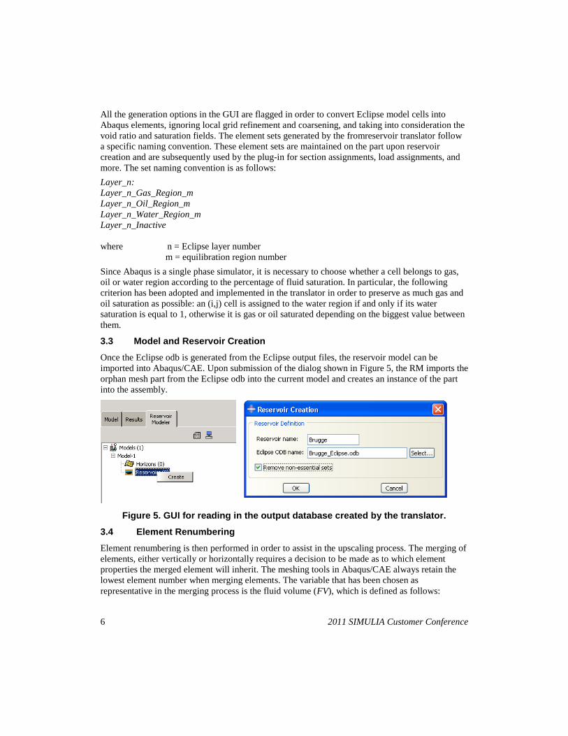
Once the Eclipse odb is generated from the Eclipse output files, the reservoir model can be

imported into Abaqus/CAE. Upon submission of the dialog shown in Figure 5, the RM imports the

orphan mesh part from the Eclipse odb into the current model and creates an instance of the part

into the assembly.

Figure 5. GUI for reading in the output database created by the translator.

3.4 Element Renumbering

Element renumbering is then performed in order to assist in the upscaling process. The merging of

elements, either vertically or horizontally requires a decision to be made as to which element

properties the merged element will inherit. The meshing tools in Abaqus/CAE always retain the

lowest element number when merging elements. The variable that has been chosen as

representative in the merging process is the fluid volume (FV), which is defined as follows:


SatPVFV

where PV = Pore Volume of the cell

Sat = Gas / Oil / Water Saturation

The plug-in renumbers elements so that elements with the most fluid volume are assigned the

lower element numbers and will thus have their material properties assigned to the merged

element.

3.5 Upscaling

A process of upscaling is necessary to improve the quality of the elements of the mesh. Upscaling

involves the merging of entire rows of elements in the horizontal direction while maintaining the

vertical discretization. This process is conducted based on the scheme specified in Table 1:

J direction

start 1 33 35 37

end 32 34 36 48

merges 4 2 1 2

Table 1-Horizontal upscaling.

Upscaling is performed using the Merge Layers item in the mesh edit tools. Selecting the icon

brings up the Edit Mesh dialog shown in Figure 6.

Figure 6. Snapshot of the GUI for performing mesh editing.

Using the same icon, the method „Grow short edges‟ is used for adjusting some elements whose

thickness was less than 2.2 cm.

The quality of the mesh is then verified; it is confirmed that no elements get flagged as erroneous.

It is then possible to carry on with the creation of the burden regions.

The renumber sche


3.6 Burden regions creation

The creation of burden regions is performed entirely outside of the plug-in. The Extrude method of

the Create Bottom-Up Mesh dialog is used to extrude layers of elements from the element faces on

the sides of the reservoir. The elements are extruded in a direction provided by the user until they

intersect chosen planes. The chosen planes can be either datum planes or horizons. The number of

layers comprising the burden regions and the associated bias can also be chosen.

For the Brugge field, datum planes are created to generate the side burden regions, and the option

of extending the original sets is selected as shown in Figure 7. This option modifies any sets that

have elements bordering the sides. The plug-in uses these modified sets to determine which parts

of the burden regions are associated with each reservoir layer. It will then generate additional new

sets which are then used for material property assignments. For this model, five layers have been

created along the four directions with a bias of 5; this bias value leads to creation of elements

whose length increases with increasing distance from the reservoir region.

Figure 7. GUI for creating side burden regions.

The original Eclipse model covers an area of approximately 3x17 km2, while the final

geomechanical model extends to 31x31 km2.

The original grid is then extruded vertically upwards and downwards so as to cover the sea-bed

region at 50 m and up to a depth of 5000 m. The model is divided into 4 layers from the top of the

reservoir up to the top surface (over-burden) and into 4 layers from the bottom of the reservoir up

to the base (under-burden) using the same Create Bottom-Up Mesh dialog. In this case, the

'Extend existing sets' is turned off, and „Create a set for new elements‟ is turned on. Using these


options, new element sets get created for the over-burden and under-burden layers. These sets will

be used later to assign material properties to the over- and under-burden regions (§3.8).

The final geomechanical model results in 83425 elements and 91792 nodes for a total of 304576

degrees of freedom.

3.7 Boundary Conditions

The external nodes belonging to the side-burden and under-burden regions have been restrained

against motion normal to the boundary surface.

Submodel boundary conditions have been used to constrain the pore pressure during the steps

created for the soils analysis.

3.8 Burden Property Assignment

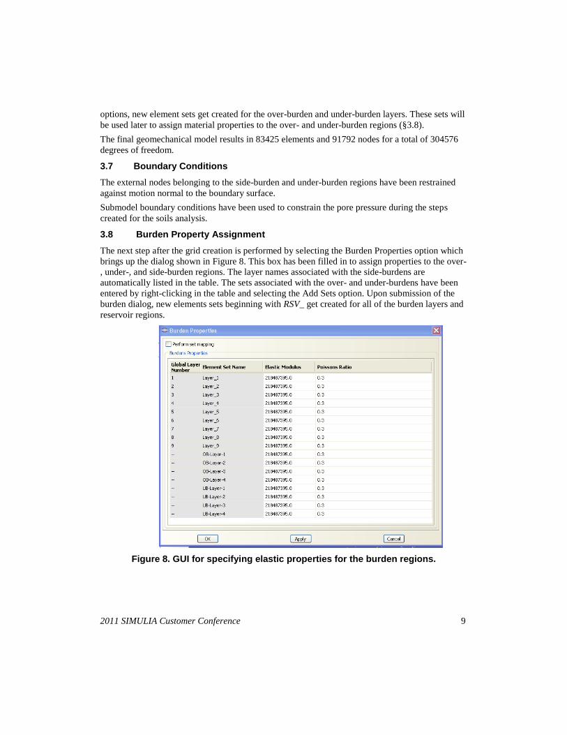
The next step after the grid creation is performed by selecting the Burden Properties option which

brings up the dialog shown in Figure 8. This box has been filled in to assign properties to the over-

, under-, and side-burden regions. The layer names associated with the side-burdens are

automatically listed in the table. The sets associated with the over- and under-burdens have been

entered by right-clicking in the table and selecting the Add Sets option. Upon submission of the

burden dialog, new elements sets beginning with RSV_ get created for all of the burden layers and

reservoir regions.

Figure 8. GUI for specifying elastic properties for the burden regions.


For the elastic simulation, a Poisson‟s ratio ( ) of 0.3 and a constant uniaxial compressibility

( cm ) of 3.40e-4 bar-1

is considered. The elastic modulus ( E ) is then computed using the

following formula:

)1(

)21()1(

cmE

The value of 2.185e8 Pa for E is then assigned to all the burden regions.

Considering plasticity, a compressibility value depending on the depth is computed for each layer

and a resulting elastic bulk modulus is obtained. These initial values are reported in Table 2 and

have been used to run the geostatic simulation. The new stress field obtained after the initialization

will then be used to automatically update these moduli as explained in §3.18.

3.9 Density Assignment

The density required for an analysis within Abaqus is referred to as dry density and is defined as

follows:

fd z)(

where d = Dry density used in *Density definition

f

= Fluid density

)(z = Bulk density

The density of the fluid, necessary to determine the overall density (dry density) that Abaqus

requires for an analysis, is calculated as follows:

g

f

f

where f = Fluid density (varies element-by-element)

= Porosity (varies element-by-element)

f = Specific weight of fluid (constant within an equilibration region)

g = Gravitational constant

The specific weight of the fluid is stored on the Eclipse odb file on an element-by-element basis

but with the same value for each element in an equilibration region. It is computed from the .DBG

Eclipse file specified in the translator dialog box. The porosity, on the other hand, is stored on an

element-by-element basis, consistent with the Eclipse values.

We assume the bulk density to vary based on depth only; it is supposed to be represented by the

mathematical expression reported in Figure 9 where 50 m represents the depth of the seabed.

2011 SIMULIA Customer Conference

11

Figure 9. Bulk Density Definitions.

Upon submission of the Bulk Density dialog, a discrete field gets calculated using the bulk density

values minus the fluid density values that is pulled from the previously described region-level

discrete fields. The discrete field will thus contain densities defined on an element-by-element

basis, and will be referenced in all of the material assignments through distributions.

3.10 Reservoir Region Properties

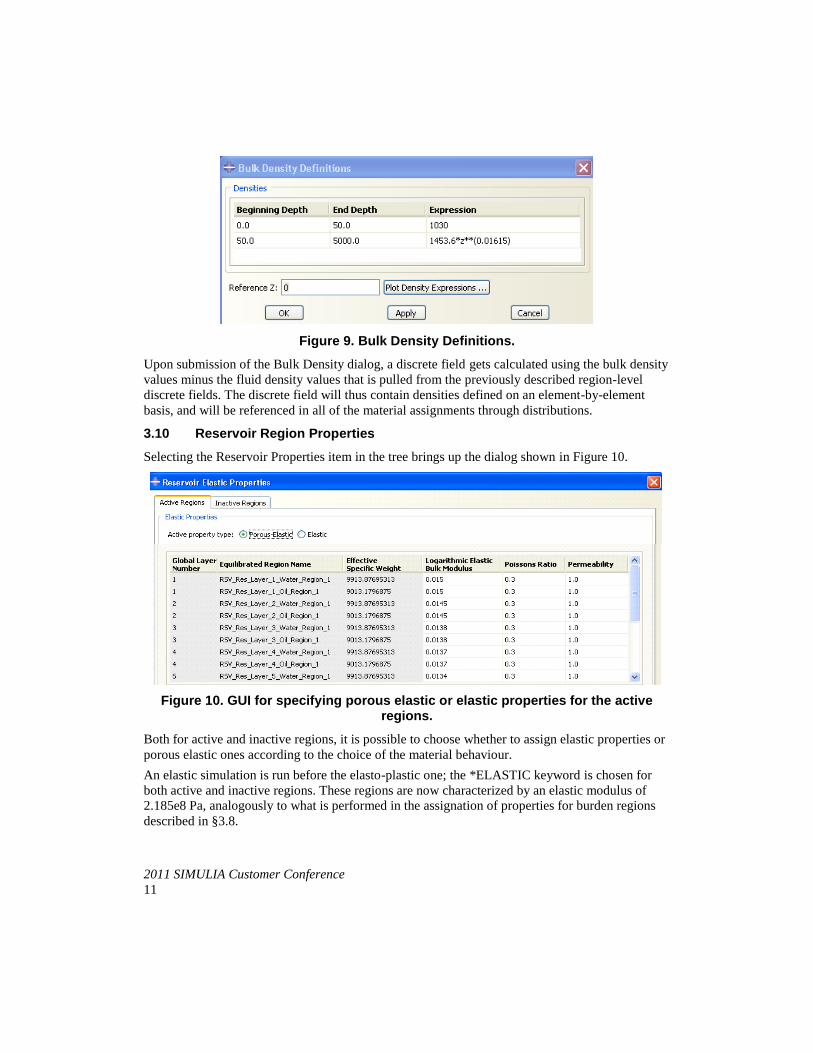
Selecting the Reservoir Properties item in the tree brings up the dialog shown in Figure 10.

Figure 10. GUI for specifying porous elastic or elastic properties for the active regions.

Both for active and inactive regions, it is possible to choose whether to assign elastic properties or

porous elastic ones according to the choice of the material behaviour.

An elastic simulation is run before the elasto-plastic one; the *ELASTIC keyword is chosen for

both active and inactive regions. These regions are now characterized by an elastic modulus of

2.185e8 Pa, analogously to what is performed in the assignation of properties for burden regions

described in §3.8.


For the plastic simulation, the *POROUS ELASTIC keyword is instead selected for the active

regions. The logarithmic elastic bulk modulus is computed for each layer according to its average

depth and vertical effective stress. The Young‟s modulus referring to each reservoir burden region

is similarly calculated and inputted. Table 2 reports the values used for the elasto-plastic

simulations.

It is important to underline that these properties will be recalculated after the reading of the

geostatic results (§3.16) in order to compare the guessed moduli with the ones obtained after

equilibrium is reached.

3.11 Pressure field computation

As already mentioned in §3.2, the translator converts finite volume results to an Abaqus output

database file. This output database file can be used to apply Eclipse generated pore pressure field

history to an Abaqus Standard analysis for performing a soils consolidation study.

To enable use in the submodeling procedure, the translator associates cell pressures with nodes.

The nodal values of the pore pressure, p̂ , are obtained by averaging and combining pore

pressures, ip , in N cells adjacent to each node. Adjacency is determined according to the method

specified for the grid translation and various methods can be chosen as well for controlling the

averaging.

For the Brugge Field, the poreweight averaging method has been specified. With this method, the

pore pressure in the output database is determined according to the expression:

N

m

m

N

m

mm PVPVpp11

ˆ

where mPV are the adjacent cell pore volumes.

Moreover, depending on the .xml configuration file, either relative or absolute pressure can be

computed and written to the odb file as pore pressure history data. Relative values are used in the

elastic simulation. They refer to the first frame field and so they are computed at time step t as

follows:

0ˆˆˆ ppp tt

Absolute pressures are instead used in the plastic simulation.

In the present study, the initial pore pressure field is specified as the one obtained from the flow

model initialization. It is also adjusted to make it consistent with the fluid contacts and the specific

weight of the saturating fluid, both of which are computed from the data values in the .DBG

Eclipse file for each equilibration region.

The pore pressure at any time step t is then calculated taking into consideration the initial pore

pressure and the relative pressure at the time step specified.

3.12 Elastic simulation

The first FE calculations are performed under the hypotheses of a linear elastic behaviour of the

material with homogeneous and isotropic mechanical properties.


13

Choosing the elastic as active property type, the GUI removes all the following items with the

exception of the assignation of initial void ratio which is directly read from the odb file.

In the analysis, the pore pressure history is defined through submodeling techniques. The input file

is written out, and the simulation is then run.

The results obtained in terms of iso-subsidence curves are shown in Figure 11 together with the

results obtained with a semi-analytical solution (Geertsma and Van Opstal, 1973) using the same

homogeneous and isotropic mechanical properties. It is evident that a very good agreement is

achieved.

-12000 -7000 -2000 3000 8000 13000 18000

-8000

-3000

2000

7000

12000

Figure 11-Iso-subsidence lines (in cm) for the elastic run at 2020: semi-analytical (black) and FE (red). The hydrocarbon saturated area of the first layer (green) and

the surrounding aquifer (blue) are also shown.

3.13 Reopen odb

After the elastic simulation is performed, it is possible to maintain the grid and mesh geometry and

run the elasto-plastic simulation using the option Reopen odb.

For this elasto-plastic analysis, one needs to use an odb file that is created using absolute pressure

conversion instead of relative pressure conversion.

The values of the elastic moduli for burden regions are then changed as described in §3.8 . The

property type Elasto-plastic is selected for active regions and different values for each layer are

assigned as explained in §3.10.

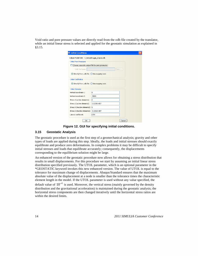
3.14 Initial Conditions

The initial conditions for void ratio, pore pressure and initial geostatic stress are applied by

selecting Initial Conditions from the plug-in and filling in the dialog box as shown in Figure 12.


Void ratio and pore pressure values are directly read from the odb file created by the translator,

while an initial linear stress is selected and applied for the geostatic simulation as explained in

§3.15.

Figure 12. GUI for specifying initial conditions.

3.15 Geostatic Analysis

The geostatic procedure is used as the first step of a geomechanical analysis; gravity and other

types of loads are applied during this step. Ideally, the loads and initial stresses should exactly

equilibrate and produce zero deformations. In complex problems it may be difficult to specify

initial stresses and loads that equilibrate accurately; consequently, the displacements

corresponding to the equilibrium solution might be large.

An enhanced version of the geostatic procedure now allows for obtaining a stress distribution that

results in small displacements. For this procedure we start by assuming an initial linear stress

distribution specified previously. The UTOL parameter, which is an optional parameter in the

*GEOSTATIC keyword invokes this new enhanced version. The value of UTOL is equal to the

tolerance for maximum change of displacements. Abaqus/Standard ensures that the maximum

absolute value of the displacement at a node is smaller than the tolerance times the characteristic

element length in the model. If the UTOL parameter is used without any value specified, the

default value of 510 is used. Moreover, the vertical stress (mainly governed by the density

distribution and the gravitational acceleration) is maintained during the geostatic analysis; the

horizontal stress components are then changed iteratively until the horizontal stress ratios are

within the desired limits.


15

Figure 13 shows the final result in terms of vertical displacement for the geostatic analysis: a ratio

of 0.54 has been specified and 5 iterations were needed to obtain the equilibrium and the final

stress distribution.

Figure 13 - Vertical displacement in the final geostatic analysis.

3.16 Geostatic Results

Upon completion of geostatic analysis, the resulting odb is read and the computed effective

vertical stresses are then used to compute the plastic properties and to update the elastic ones.

3.17 Plastic Property Assignments

Selecting the Update Properties item, it is possible to define on a region-by-region basis the

quantities that are required for the *CLAY PLASTICITY definition. Additional coefficients

and are required to compute the compressibility as a function of the vertical effective stress .

The relationship is as follows:

cm

The compressibility is then used to calculate the logarithmic plastic bulk modulus as follows:

)1(cm

where refers to the element void ratio.

The computations of compressibility and logarithmic plastic bulk modulus are performed on an

element-by-element basis, and then averaged over the entire equilibration region.

For the inactive reservoir regions and burden regions, the elastic modulus E

is computed as

follows:


(1 ) (1 2 )

(1 )E

cm

The logarithmic elastic bulk modulus K is then computed by the relationship: / 3K . The

values used for the plastic simulation are reported in Table 2:

Elastic

modulus [Pa-1

]

Logarithmic

Elastic Bulk

Modulus

Logarithmic

Plastic Bulk

Modulus

Compressibility

Coefficient

Compressibility

Coefficient

Layer 1 1.95E+08 0.015 0.045 0.262 1.122

Layer 2 2.01E+08 0.015 0.044 0.277 1.127

Layer 3 2.06E+08 0.014 0.042 0.293 1.131

Layer 4 2.12E+08 0.014 0.041 0.310 1.136

Layer 5 2.18E+08 0.013 0.040 0.328 1.141

Layer 6 2.25E+08 0.014 0.043 0.348 1.146

Layer 7 2.32E+08 0.014 0.042 0.368 1.151

Layer 8 2.40E+08 0.014 0.041 0.390 1.156

Layer 9 2.48E+08 0.012 0.036 0.420 1.163

Over-burden 1 1.73E+08 0.020 0.898

Over-burden 2 1.55E+08 0.030 0.932

Over-burden 3 1.40E+08 0.068 1.005

Over-burden 4 1.28E+08 1.741 1.286

Under-burden 1 2.97E+08 0.032 0.938

Under-burden 2 3.71E+08 0.029 0.931

Under-burden 3 4.95E+08 0.034 0.945

Under-burden 4 7.43E+08 0.049 0.977

Table 2- Values used for the plastic simulation.

3.18 Property Overrides

The logarithmic elastic and plastic bulk moduli are then recomputed using the vertical stress

obtained after the geostatic step. By clicking on the Update Properties in the tree and then

selecting the Override Moduli option, the user can compare the values assigned before and after

the geostatic step in order to investigate the effects due to the stress field obtained to reach the

equilibrium. Moreover, the user has the ability to override the properties manually; the user can

retain the initially assigned values, or can reassign other different values.

The results obtained for the Brugge field are not too different with respect to the moduli assigned

before the geostatic step; for a comparison, some of them are shown in Figure 14.


17

Figure 14 - Comparison between the original and the computed logarithmic elastic bulk modulus.

The computed moduli have therefore been maintained. The plastic simulation is then run at

different time steps; Figure 15 shows some results obtained in terms of vertical displacement.

2018 2020

2024 2028

2018 2020

2024 2028

2018 2020

2024 2028

Figure 15 - Vertical displacement at the top of the first reservoir layer at different years.


4. Conclusions

This paper describes how the new capabilities of Abaqus 6.11 in combination with the RM plug-in

have allowed for an automation of the workflow used to perform a geomechanical analysis on a

field scale model directly in Abaqus/CAE.

In particular, the following new functionalities in Abaqus 6.11 have been used:

The translator which establishes a link between Eclipse and Abaqus/CAE. All the

information from the reservoir model in terms of grid, properties and pressure are

transmitted to the FE model, which is then populated by these data in a completely

consistent way.

The meshing tools for adjusting elements and nodes where needed and for performing

upscaling. Moreover the burden region creation was properly done through these

capabilities.

The automated geostatic procedure.

The assignation of material properties and load history automatically within Abaqus/CAE

to run both the elastic and elasto-plastic simulations

In addition to these new capabilities, the GUI allows for following a logical scheme in order to

easily and automatically executing all the steps required in the creation of a geomechanical model.

The possibility to clearly have a sequence of steps to be performed significantly improves the

efficiency in terms of user time of the preprocessing phase needed to build a full field

geomechanical model.

The new capabilities implemented in Abaqus/CAE and the RM plug-in have then shown to be

particularly appropriate for reservoir geomechanical simulations. The analysis can now be more

proper and precise, and the automation allows for shortening the time required to setup and run

reservoir geomechanics simulation models.

5. References

1. Abaqus User‟s manual 2011.

2. Boot, R., “Level Control Surveys in the Groningen Gas Field”, Verhandelingen Kon. Ned.

Geol. Mijnbouwk. Gen., Vol. 28, pp. 105-109, 1973.

3. Bruno, M. S., “Subsidence-Induced Well Failure”, SPE Drilling Engineering, 1992.

4. Capasso G., Mantica S., “Numerical Simulation of Compaction and Subsidence Using

Abaqus”, AUC, 2006.

5. Da Silva, F. W., Debande G. F., Pereira C. A., and Plischke B., “Casing Collapse Analysis

Associated With Reservoir Compaction and Overburden Subsidence”, SPE 20953, 1990.

6. Floris, F.J., Bush, M.D., Cuypers, M., Roggero, F., and Syversveen, A.R., “Comparison of

Production Forecast Uncertainty Quantification Methods - An Integrated Study”, paper

presented at 1st Conference on Petroleum Geostatistics, Toulouse 1999.


19

7. Geertsma, J., “A Basic Theory of Subsidence due to Reservoir Compaction: the

Homogeneous Case”, Verhandelingen Kon. Ned. Geol. Mijnbouwk. Gen., Vol. 28, pp. 43-62,

1973.

8. Geertsma J. and Van Opstal G., “A Numerical Technique for Predicting Subsidence Above

Compacting Reservoirs Based on the Nucleus of Strain Concept”, Verhandelingen Kon. Ned.

Geol. Mijnbouwk. Gen., Vol. 28, pp. 63-78, 1973a.

9. Mindlin R.D. and Cheng D.H., “Thermoelastic Stress in the Semi-Infinite Solid”, J. of

Applied Physics, Vol. 21, p. 931-933, 1950.

10. Ostermeier, R. M., “Deepwater Gulf of Mexico Turbidites – Compaction effects on Porosity

and Permeability”, SPE 26468, 1995.

11. Schlumberger, “Eclipse Reference Manual 2009”, 2009.

12. The BRUGGE Field, http://www.isapp.nl/brugge-field-case

13. Terzaghi, K., “The Shearing Resistance of Saturated Soils and the Angle Between the Plane

of Shear”, Proc. of 1st Int. SMFE Conference, Harvard Mass., Vol.1, pp. 54-56, 1936.

14. Zaman, M. M., Abdulrahheem, A. and Roegiers, J. C., “Reservoir Compaction and Surface

Subsidence in the North Sea Ekofisk field”, Subsidence due to fluid withdrawal, Elsevier

Scince, pp. 373-419, 1995.

6. Acknowledgments

The two years fruitful and productive cooperation with Simulia US and Simulia Italia allowed for

developing the work presented in this paper. The authors are very grateful to all the developers

from Simulia who took part on this project implementing new capabilities in the code to enable

this new workflow. In particular, Jeff Haan and his team for developing the translator, Matthew

Rees and Konstantin Kovalev for creating new mesh editing tools and Mike Shubert for creating

the Reservoir Modeler Extension. The contribution of each of them has been necessary and

fundamental for the good outcome of the project.

Field Scale Geomechanical Modelling Using a New Automated ...

Documents

Transcript of Field Scale Geomechanical Modelling Using a New Automated ...