Field Guide and Data Collection Procedures...

Field Guide and Data Collection Procedures (Appendix 1)

Riverine and Slope River Proximal Wetlands in Coastal Southeast & Southcentral Alaska

Operational Draft Guidebook Using the HGM Approach

By: Jim Powell, David D’Amore, Ralph Thompson, Terry Brock, Pete

Huberth, Bruce Bigelow, and M. Todd Walter

Prepared For: State of Alaska, Department of Environmental Conservation

410 Willoughby Ave., Suite 303 Juneau, AK 99801

June 2003

Field Guide and Data Collection Procedures Riverine and Slope River Proximal Wetlands in Coastal Southeast & Southcentral Alaska Operational Draft Guidebook Using the HGM Approach

By: Jim Powell Terry Brock

Wetlands Program Coordinator Soil and Wetland Scientist Division of Air and Water Quality

PWS (retired) USDA Forest Service

Alaska Department of Environmental

Juneau, AK 99801

Conservation 410 Willoughby Ave., Suite 105 Bruce Bigelow Juneau, AK 99801-1795 Hydrologist

David V. D'Amore

U.S. Geological Survey Water Resources Division

Research Soil Scientist Juneau, AK 99801 USDA Forest Service, Pacific Northwest Pete Huberth Research Station 2770 Sherwood Lane,

Forester Forestry Industry Consulting

Suite 2A 6725 Marguerite Street Research Position Juneau, AK 99801

Juneau, AK 99801-9431

Ralph Thompson Todd Walter

Biologist / PWS (Former Position) Juneau Regulatory Field Office

Affiliate Professor, University of Alaska Southeast 11120 Glacier Highway

Regulatory Branch Juneau, AK 99801 U.S. Army Corps of Engineers Senior Research Associate Suite 106, Jordan Creek Center 8800 Glacier Highway

Cornell University Dept. of Biological &

Juneau, AK 99801 Environmental Eng. Ithaca, NY 14853-5701

This document should be cited as: Powell, J.E., D. V. D’Amore, R. Thompson, T. Brock, P. Huberth, B. Bigelow, and M. T. Walter. “Field Guide and Data Collection Procedures for the Wetland Assessment Guidebook, (Appendix 1), Operational Draft Guidebook for Assessing the Functions for Riverine and River Proximal Slope Wetlands in Coastal Southeast and Southwestern Alaska Using the HGM Approach,” State of Alaska Department of Environmental Conservation June 2003 / U.S. Army Corps of Engineers Waterways Experiment Station Technical Report: WRP-DE-__.

Acknowledgments The authors wish to thank all those who helped collect the data and develop the models that are the basis for the field procedures contained in this field guide. The development of this field guide and hydrogeomorphic models requires extraordinary cooperation among many different individuals with diverse knowledge and backgrounds. Expertise in wetland ecology, soil science, hydrology, plant ecology, fish and wildlife biology, statistics, land use, and other disciplines is needed to produce scientifically sound models, which form the basis of the hydrogeomorphic (HGM) functional assessment methodology. In addition, the building of an HGM model requires skill in personnel and funding management as a project usually involves many agencies (state, federal, and local) and private organizations. The agencies and groups providing direct funding, personnel, and logistical support for this project include:

Alaska Department of Natural Resources (ADNR)

USDA Natural Resources Conservation Service (NRCS) U.S. Environmental Protection Agency (EPA) U.S. Army Corps of Engineers (COE) USDA Forest Service (USFS) USDA U.S. Forest Service, Pacific Northwest Research Station Alaska Department of Fish and Game (ADF&G) U.S. Geological Survey, Water Resources Division (USGS) Alaska Department of Environmental Conservation (ADEC).

EPA, Alaska Operations Office, provided the majority of the funding for this project through ADEC.

A great deal of field time and technical support were provided by local wetland experts including Ms. Janet Schempf (ADF&G), Dr. K Koski (NMFS), Mr. Kevin Brownlee (ADF&G), Rick Noll (formerly of ADNR), Mr. Mark Anderson (ADEC), Ms. Ann Leggett (HDR Alaska, Inc.), and Mr. Mark Jen (EPA). Mr. Jack Gustafson and Mr. Dave Hardy (ADF&G) provided local knowledge and expertise in Sitka and Ketchikan, Alaska. Chugachmuit Native Association also provided logistical support in Port Graham and Nanwalik, Alaska.

Furthermore, the authors greatly appreciated the considerable talent and effort Dr. Mark Brinson, Mr. Garrett Hollands, Dr. Lyndon C. Lee, Dr. Wade Nutter,

and Dr. Dennis Whigham provided in terms of field time and technical reviews of the initial draft.

Disclaimer This field guide is the same as Appendix 1 in the “Operational Draft Guidebook For Assessing the Functions of Riverine and Slope River Proximal Wetlands in Coastal Southeast & Southcentral Alaska.”

This field guide was developed for applying an HGM functional assessment model of riverine wetlands and slope river proximal wetlands in Coastal Southeast and Southcentral Alaska. It is intended to be used in its present form consistent with the National Action Plan to Develop the Hydrogeomorphic Approach for Assessing Wetland Functions (Federal Register, August 16, 1996 (Vol. 61, No. 160) at page 42603). This field guide and the Operational Draft Guidebook upon which it is based will be used and reviewed for a two-year period by regulatory and resource agencies. Other organizations, and other parties will have an opportunity to use the Operational Draft Guidebook during this two-year period and provide recommendations for improvement. After the Operational Draft Guidebook has been used in the field for two years it may be revised incorporating comments and corrections identified by the Guidebook Development Team. The revised Operational Draft Guidebook will be reviewed and approved by the COE/WES as a Final Guidebook.

Jim Powell Wetlands Program Coordinator Alaska Department of Environmental Conservation

ladkladkfj

Contents

Preface.............................................................................................1

Purpose of this Field Guide .......................................................................... 1

How to use this Field Guide ..........................................................2

Procedure for Developing an HGM Rapid Assessment Report:................... 3

Functional Assessment Report for Riverine and Slope River Proximal Wetlands Using the HGM Approach ..........................4

Six-Step Process for Developing an HGM Functional Assessment Report.. 4 Step 1. Preliminary HGM Classification .................................................... 6 Step 2. Site Information (Completed in the Field or Office) ....................... 8 Step 3. Sketch a map of Project Assessment Area......................................10 Step 4 (a) Summary of Riverine Variables ..................................................11

Riverine Wetlands........................................................................14 1) Median Pebble Size D50 (Vpebble-D50): .................................. 15 2) Channel Roughness (Vchanrough D84): .................................... 16 3) Embeddedness (Vembedded): .................................................... 184) Potential for Coarse Wood (Vcwpot): ........................................ 185) In - Channel Coarse Wood (Vcwin) ........................................... 19 6) Log jams (Vlogjams) ....................................................................20 7) Subsurface Flow into the Water/Wetland (Vsubin).................... 20 8) Riparian Shade (Vshade) .............................................................219) Alterations of Hydroregime (Valthydro) .................................... 23 10) Barriers to Fish Movement (Vbarrier) ........................................ 24 11) Frequency of Overbank Flooding (Vfreq ) ................................. 25 12) Flood Prone Area Storage Volume (Vstore)................................2713) Soil Permeability (Vsoilperm) .................................................... 28 14) Tree Basal Area (Vtreeba) .......................................................... 29 15) Total Vegetative Cover (Vvegcov)..............................................3016) Number of Vegetative Strata (Vstrata) ....................................... 33 17) Land Use of Project Assessment Area (Vwetuse) ...................... 35 18) Land use of the Watershed (Vwatersheduse)............................. 36

Step 4 (b) Summary of Slope River Proximal Variables ............................ 38 HGM Asessment Area: Slope River Proximal Wetlands ............................39

Slope Riverine Proximal Wetlands. ...........................................40 1) Presence of Redoximorphic Features (Vredox).......................... 40 2) Presence and Structure of the Acrotelm Horizon (Vacro) .......... 41 3) Soil Permeability (Vsoilperm)......................................................42 4) Water Sources (Vsource)............................................................ 42 5) Subsurface Flow From the Wetlands (Vsubout)......................... 43 6) Overbank Flood Frequency (Vfreq) ........................................... 44 7) Flood Prone Area Storage Volume (Vstore)............................... 46 8) Land Use of the Project Assessment Area (Vwetuse) ................ 47 9) Adjacent Land Use (Vadjuse)..................................................... 48 10) Microtopographic Features V(micro) ........................................ 50 11) Presence of Surface Water (Vsurwat)......................................... 53 12) Total Vegetative Cover (Vvegcov)............................................. 54 13) Number of Vegetative Strata (Vstrata) ...................................... 5814) Canopy Gaps (Vgaps)................................................................ 59 15) Basal of Area of Trees (Vtreeba)................................................ 60 16) Log Decomposition (Vdecomp) ................................................. 61 17) Number of Coarse Wood (Vcwslope) .........................................62

Step 5a. Variable Scoring Sheet - Riverine ............................................... 64 Step 5b. Variable Scoring Sheet. – Slope River Proximal............................65 Step 6a. Functional Scoring Sheets - Riverine .......................................... 66 Step 6.b Functional Scoring Sheet - Slope Riverine Proximal .................. 67

HGM Rapid Assessment Report Data Collection Sheets .........68

Preface

Purpose of this Field Guide This field guide is intended to provide guidance and field procedures necessary for completing a rapid assessment report using the HGM approach. It is also designed to supplement the Operational Draft Guidebook for riverine wetlands, and slope river proximal wetlands on low permeability deposits and bedrock in Coastal Southeastern and Southcentral Alaska. This field guide is included in the Operational Draft Guidebook as Appendix 1.

The field guide is designed to be used in the field with the equipment suggested on thefollowing page.

Suggested Equipment List

1 100 ft Measuring Tape (English units)

1 Soil Color Chart (i.e. Munsell Soil Chart)

1 Prism or angle gauge measurement for measuring the basal area of trees

1 Flagging: one to two rolls

1 Shovel (sharp shooter or soil spade)

1 6 inch transparent measurement ruler (metric)

1 Small measuring tape (metric)

2 Small wooden or tent stakes

1 Waterproof hip boots

1 DBH measuring tap (English units)

1 Handheld calculator

1 Plant identification key

How to use this Field Guide This field guide is designed to be used in the field as a reference for collecting the necessary information to rapidly assess wetland functions for riverine and slope river proximal wetlands in Southcentral and Southeast Alaska. If you are familiar with the Hydrogeomorphic Approach and have a copy of the Operational Draft Guidebook for Riverine and Slope River Proximal (http://www.state.ak.us/dec/dawq/nps/wetlands.htm#WET5) the following procedure can be used to develop a HGM Rapid Assessment Report. This report can be used for designing projects, determining mitigation and for fulfilling the requirements for functional assessments for permitting wetland projects.

Procedure for Developing an HGM Rapid Assessment Report: A) Copy the Field Data Collection Sheets For ease of collecting data and

assembling the HGM Rapid Assessment Report the sheets used for recording data and information are located at the end of this field guide. Copy these sheets on rain resistant paper:

Field Data Collection Sheets: 1) Step 1. Preliminary HGM Classification 2) Step 2. Site Information (completed in the office or field)

3) Step 3. Sketch a Map of Project Assessment Area.

4) Pebble Count & Embeddedness Work Sheet 5) Variable (15) Vegetative Cover (Vvegcov) worksheets.

6) Variable and Functional Scoring Sheets (4 pgs. in all) located at

the end of this field guide. These sheets are for recording your results and information collected from the field.

B) Follow the Six -Step Process for Developing an HGM Functional

Assessment Report outlined on the following pages.

C) After completing the Six-Step Process and calculating the Functional Capacity Indexes (FCIs), assemble the Field Data Collection Sheets into one report. This constitutes an HGM rapid assessment report.

Functional Assessment Report for Riverine and Slope River Proximal Wetlands Using the HGM Approach

Six-Step Process for Developing an HGM Functional Assessment Report Before conducting a functional assessment you need to determine if the Project Assessment Area includes jurisdictional wetlands and the type or subclass of wetlands you are assessing. The key on the next page is designed to help in determining if this field guide is appropriate for the type of wetlands you are assessing (i.e., riverine or slope river proximal wetlands). After you have determined that you are assessing riverine and/or river proximal wetlands then the following six-step process can be used to complete a report for a rapid assessment for these wetlands. (Note: If the assessment area includes both wetland classes then the following six-step process is required for each class).

Six-Step Process

1. Conduct a Preliminary HGM Classification. 2. Complete the Site Information Sheet. 3. Sketch a map of the Project Assessment Area. 4. Collect the field measurements for each variable and record them in the

field measurement column of the Variable Scoring Sheet.

5. Determine the variable score using the field measurements and the variable index scoring table. Record the variable score in the Variable Index score column of the Variable Scoring Sheet.

C) Determine the Functional Capacity Index (FCI) of each function by entering

the appropriate score into an electronic spreadsheet (included in the Operational Draft Guidebook’s appendices). Or, manually calculate the score using the Functional Scoring Shee t. A copy of the electronic spreadsheet th at is av ailable on the State of Alaska, Department of Environmental Conservation website: (http://www.state.ak.us/us/dec/dawq/nps/wetlands.htm#wet5).

Key to Riverine & Slope River Proximal Wetlands in Coastal SE & SC Alaska

1a. The assessment area is not a jurisdictional wetland according to the Corps of Engineers Wetland Delineation Manual (U.S. Army Corps of Engineers 1987). For example, (1) the area is a deepwater aquatic habitat. Deepwater aquatic habitats are areas that are permanently inundated at mean annual water depths > 6.6 ft or permanently inundated areas ≤ 6.6 ft that do not support rooted-emergent or woody plant species: Non-wetland: Guidebook not applicable.

1b. The assessment area is a jurisdictional wetland according to the Corps of Engineers Wetland Delineation Manual: 2

2a. The wetland is tidally influenced, glacially driven water source, in a closed depression (e.g., pothole on glacial moraine), or is adjacent to a lake where the water elevation of the lake maintains the water table in the wetland: Guidebook not applicable.

2b. The wetland is a river or within 200 feet adjacent to a river : go to 3

3a. The slope of the land or water surface exceeds 25%: Guidebook not applicable.

3b. The slope of the land or water surface 0.002 ≤ 25%: go to 4

4a. The wetland is located in valley bottoms, within 200 feet of the bankfull of a river channel, and ground or surface waterflow driven. YES. Use the Slope River Proximal Subclass in this guidebook.

4b. The wetland is in an active river channel, a higher order stream reach derived from non-glacial water sources, occurring on valley bottoms, and corresponds with Rosgen Stream types “B” or “C” and USFS Tongass National Forest Channel Types 1) Moderate Gradient Mixed Control, 2) Moderate Gradient Contained, or 3) Flood Plain process groups. YES. Use the Riverine Subclass in this guidebook.

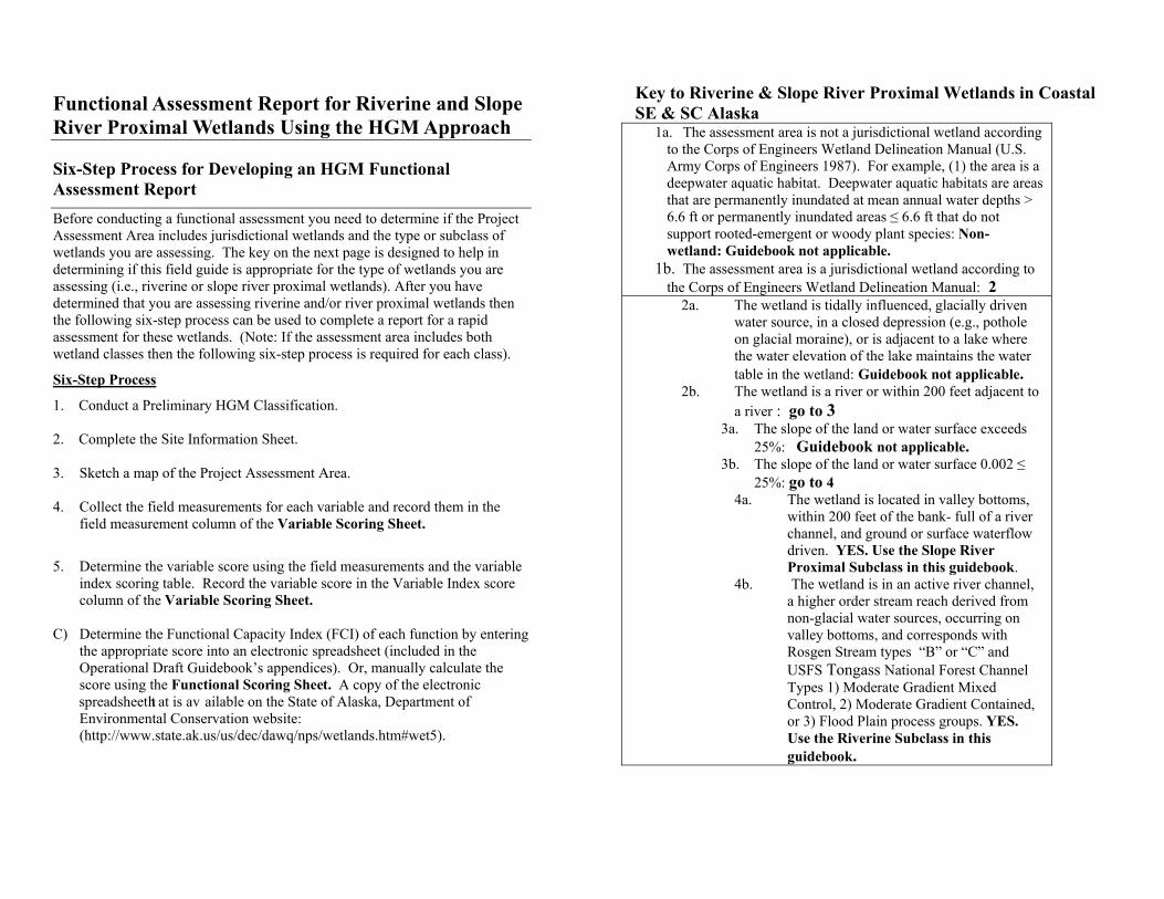
Step 1. Preliminary HGM Classification Identify, verify, and document the rationale used for recognizing HGM classes and subclasses within the project assessment area. Determine if the assessment area is a RIVERINE and/or SLOPE RIVER PROXIMAL Wetland Subclass by using the dominant characteristics outlined below. Show how the project assessment area satisfies a subclass definition provided in the guidebook by completing the form below. Specifically, include a discussion of the site characteristics and show how they are consistent with the dominant characteristics of the subclass.

Riverine Wetland Dominant Characteristics CHARACTERISTIC DESCRIPTION Hydrologic Source Unidirectional flow, higher order streams, derived

from non-glacial water sources

Vegetation Any vegetation life form (e.g., trees, shrubs, herbaceous, etc.) that are not in a marine, or estuarine system, nor directly influenced (i.e., actively flooded) by those systems.

Landforms Occur in valley bottoms, flow predominantly on bedrock, glacial till or glacial marine deposits. Low elevation stream reaches may flow on Pleistocene or Holocene alluvial gravel deposits, or deltaic estuarine deposits raised in elevation by tectonic lift.

Slope 0.001% to ≤ 2.2% Parent Materials Upper reaches: exposed bedrock, glacial till,

and colluvium over bedrock, alluvial sand, and gravel. Lower reaches: dense basal till, marine lucustrine and glacial fluvial sediments, and alluvial sand and gravel.

Soils Sand, silt, and gravel deposits with occasional surface organic matter accumulation.

Provide the site Characteristics:

Hydrologic Source Vegetation Landform, soils Slope

Slope River Proximal Wetland Dominant Characteristics CHARACTERISTIC DESCRIPTION

Location Located within 200 feet of the bankfull of a river channel.

Hydrologic Source Ground or surface water flow. Vegetation Any vegetation life form (e.g., trees, shrubs,

herbaceous, etc.) that are not in a marine, or estuarine system nor directly influenced (i.e., actively flooded) by those systems.

Landforms Occur adjacent to streams and valley sides. Occur in valley bottoms, flow predominantly on bedrock, glacial till or glacial marine deposits. Low elevation stream reaches may flow on Pleistocene or Holocene alluvial gravel deposits, or deltaic estuarine deposits raised in elevation by tectonic lift. Note: wetlands in closed depressions are out of the subclass.

Slope 0.1% to ≤25% Parent Materials Upper reaches: exposed bedrock, thin till, and

colluvium over bedrock. Lower reaches: dense basal till deposited by flowing glacial ice, outwash, gravel.



Hydrologic Source

Vegetation

Landform

Slope

Parent Materials

Soils

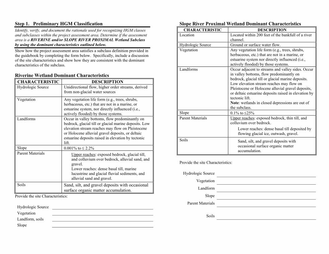
Step 2. Site Information (Completed in the Field or Office)

Dates of Site Visit

Team Members

Field Notes/Observations

Collect and review information relevant to the site. This includes, but is not limited to: USGS, state, local, and other maps (at various scales) Geotechnical, soils, or environmental reports Correspondence, construction plans on the proposed project Published literature

Identify the documents that were collected and reviewed. Include a detailed description of each document (e.g., citation, date, scale, quadrangle name, etc.). If possible, attach copies of each document.

USGS, state, borough, and other maps (at various scales):

1. ______________________________________________

2. ______________________________________________

Air photos and other imagery: 1. ______________________________________________

2. ______________________________________________

Relevant geotechnical, soils, or environmental reports: 1. ______________________________________________

2. ______________________________________________

• Correspondence, construction plans, and specifications, etc. on the proposed project:

______________________________________________________

Relevant published literature: ______________________________________________________

Other documents:

Other Questions:

Is a cataloged anadromous fish stream adjacent to or part of the assessment area?

Is the assessment area used by any federally listed threatened or endangered species?

Is the assessment area adjacent to a state listed impaired waterbody? Is the assessment area listed as a historic or cementary?

Step 3. Sketch a map of Project Assessment Area

Image source, date, and scale: ____________________________

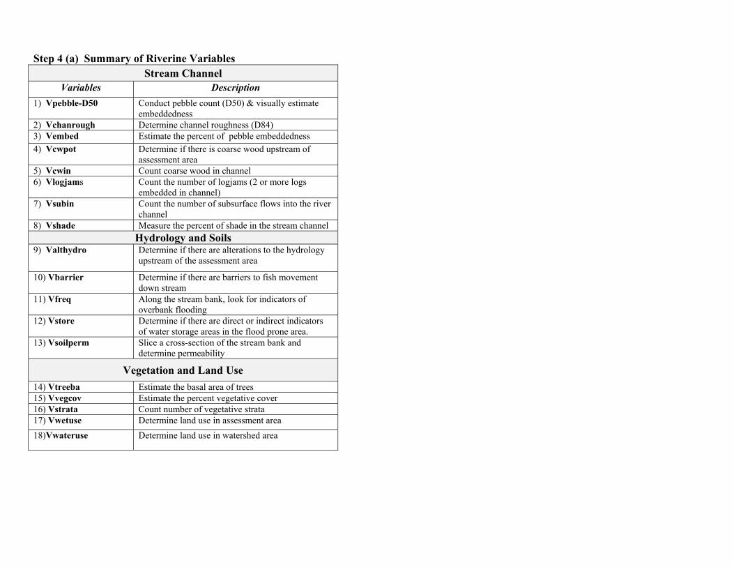
Step 4 (a) Summary of Riverine Variables Stream Channel

Variables Description 1) Vpebble-D50 Conduct pebble count (D50) & visually estimate

embeddedness 2) Vchanrough Determine channel roughness (D84) 3) Vembed Estimate the percent of pebble embeddedness 4) Vcwpot Determine if there is coarse wood upstream of

assessment area 5) Vcwin Count coarse wood in channel 6) Vlogjams Count the number of logjams (2 or more logs

embedded in channel) 7) Vsubin Count the number of subsurface flows into the river

channel 8) Vshade Measure the percent of shade in the stream channel

Hydrology and Soils 9) Valthydro Determine if there are alterations to the hydrology

upstream of the assessment area

10) Vbarrier Determine if there are barriers to fish movement down stream

11) Vfreq Along the stream bank, look for indicators of overbank flooding

12) Vstore Determine if there are direct or indirect indicators of water storage areas in the flood prone area.

13) Vsoilperm Slice a cross-section of the stream bank and determine permeability

Vegetation and Land Use

14) Vtreeba Estimate the basal area of trees 15) Vvegcov Estimate the percent vegetative cover 16) Vstrata Count number of vegetative strata 17) Vwetuse Determine land use in assessment area 18)Vwateruse Determine land use in watershed area

Stream Channel Cross-section and Measurements

NOTE: 1) The floodprone area is the area defined by the projection of a plain at twice the bankfull thalweg depth. 2) In some instances, the floodprone, as defined by the projection of a plain at 2X bankful thalweg depth, will extend into areas that are slope wetlands. Riverine waters/wetlands include those areas that are predominated by fluvial processes (i.e., uni-directional flow, overbank flooding). Slope river proximal wetlands are those areas that are dominated by ground water flow.

Figure 1. HGM Assessment Area Diagram for Riverine Wetlands

900 Arc of Disturbance 1000 ft Watershed Assessment Area For (Vwatersheduse) (90 degree upstream of the Project Assessment Area) 100 ft

.10 Ac. Point Center Quarter Bankfull

Stream Channel 50 ft Channel Transect (Vcwpot)

100 ft 37.5 ft

Project Assessment Area

Stars represent flagging

Water Flow

BankfullThalwegDepth

Extent of Floodprone Area(2X Bankfull Thalweg Depth)

Floodplain SurfaceBankfull

Twice (2X)Bankfull ThalwegDepth

}} Floodplain Surface

(200 ft )SlopeRiverProximal Wetland

(200 ft)Slope River ProximalWetland

Riverine Waters / Wetland

Establish a Channel Transect and Assessment Area (Figures 1 & 2) Mark the channel bankfull width at one side of the stream and extend a measuring tape to the opposite side to establish the cross channel transect. The channel transect should be perpendicular to the stream flow. Measure upstream and downstream 100 ft from the cross channel transect to establish the assessment area. The assessment area will be referred to as such for variable measurement below.

Riverine Wetlands Stream Channel Measurements

1) Median Pebble Size D50, (VpebbleD50) 2) Channel Bed Roughness (Vchanrough) 3) Embeddedness (Vembedded) 4) Potential Coarse Wood (Vcwpot) 5) In-Channel Coarse Wood (Vcwin) 6) Logjams (Vlogjams) 7) Subsurface Flow (Vsubin) 8) Characteristic Riparian Shade (Vshade) For each variable:

a. Collect field measurements as directed below and record them in the field measurement column of the Variable Scoring Sheet.

b. Determine the variable score using the field measurements and the variable index scoring table. Record the variable score in the Variable Index score column of the Variable Scoring Sheet.

c. Determine the Functional Capacity of each function by entering the appropriate score into an electronic spreadsheet included in the Operational Draft Guidebook’s Appendices. Or, manually calculate the score using the Functional Scoring Sheet.

Pebble Count:

Take a random walk in the stream channel within the assessment area. While taking the walk, occasionally stop and plant your right foot. Over the toe of your right boot and with eyes closed or averted, touch an extended finger to the nearest rock or sand grain (includes: gravel, cobble, and boulders >2mm). Pick

up the rock or sand, and using a transparent ruler measure along the intermediate axis (i.e. neither the longest nor the shortest). Record your measurements in millimeters (mm) in the appropriate size class. (Table 4). Start at the bottom of each size class and fill in each row. (Dunne and Leopold, 1978). In doing so, you are constructing a "histogram" (bar chart) that shows the size distribution of the inorganic stream bed materials. The pebble count is used for scaling two variables: Median Pebble Size D50 (VpebbleD50) and Channel Bed Roughness (Vchanrough). Also, during the pebble count determine the percent of sediment surrounding the nearest pebble rock or sand grain for scaling embeddedness (Vembedded).

1) Median Pebble Size D50 (Vpebble-D50): Determine the median pebble size (D50) of the samples by using the Pebble Count Table following the procedure outline above.

Pebble Count & Embeddedness Work sheet

>2 2-4 5-8 9-16 17-32 33-64 65-128

129-256

257-512

512- 1024 > 1024

Embeddness Work Sheet

0 – 25% 26 – 50% 51 – 75% 76 – 100%

Examples of embedded pebbles:

< 25% 75 – 100% 51 – 75% 25 - 50%

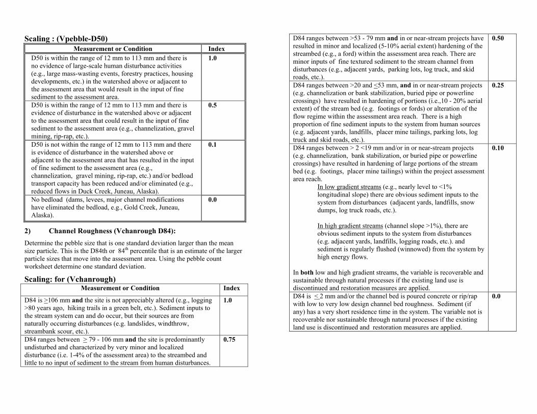
Scaling : (Vpebble-D50) Measurement or Condition Index

D50 is within the range of 12 mm to 113 mm and there is no evidence of large-scale human disturbance activities (e.g., large mass-wasting events, forestry practices, housing developments, etc.) in the watershed above or adjacent to the assessment area that would result in the input of fine sediment to the assessment area.

1.0

D50 is within the range of 12 mm to 113 mm and there is evidence of disturbance in the watershed above or adjacent to the assessment area that could result in the input of fine sediment to the assessment area (e.g., channelization, gravel mining, rip-rap, etc.).

0.5

D50 is not within the range of 12 mm to 113 mm and there is evidence of disturbance in the watershed above or adjacent to the assessment area that has resulted in the input of fine sediment to the assessment area (e.g., channelization, gravel mining, rip-rap, etc.) and/or bedload transport capacity has been reduced and/or eliminated (e.g., reduced flows in Duck Creek, Juneau, Alaska).

0.1

No bedload (dams, levees, major channel modifications have eliminated the bedload, e.g., Gold Creek, Juneau, Alaska).

0.0

2) Channel Roughness (Vchanrough D84): Determine the pebble size that is one standard deviation larger than the mean size particle. This is the D84th or 84th percentile that is an estimate of the larger particle sizes that move into the assessment area. Using the pebble count worksheet determine one standard deviation.

Scaling: for (Vchanrough) Measurement or Condition Index

D84 is >106 mm and the site is not appreciably altered (e.g., logging >80 years ago, hiking trails in a green belt, etc.). Sediment inputs to the stream system can and do occur, but their sources are from naturally occurring disturbances (e.g. landslides, windthrow, streambank scour, etc.).

1.0

D84 ranges between > 79 - 106 mm and the site is predominantly undisturbed and characterized by very minor and localized disturbance (i.e. 1-4% of the assessment area) to the streambed and little to no input of sediment to the stream from human disturbances.

0.75

D84 ranges between >53 - 79 mm and in or near-stream projects have resulted in minor and localized (5-10% aerial extent) hardening of the streambed (e.g., a ford) within the assessment area reach. There are minor inputs of fine textured sediment to the stream channel from disturbances (e.g., adjacent yards, parking lots, log truck, and skid roads, etc.).

0.50

D84 ranges between >20 and <53 mm, and in or near-stream projects (e.g. channelization or bank stabilization, buried pipe or powerline crossings) have resulted in hardening of portions (i.e.,10 - 20% aerial extent) of the stream bed (e.g. footings or fords) or alteration of the flow regime within the assessment area reach. There is a high proportion of fine sediment inputs to the system from human sources (e.g. adjacent yards, landfills, placer mine tailings, parking lots, log truck and skid roads, etc.).

0.25

D84 ranges between > 2 <19 mm and/or in or near-stream projects (e.g. channelization, bank stabilization, or buried pipe or powerline crossings) have resulted in hardening of large portions of the stream bed (e.g. footings, placer mine tailings) within the project assessment area reach.

In low gradient streams (e.g., nearly level to <1% longitudinal slope) there are obvious sediment inputs to the system from disturbances (adjacent yards, landfills, snow dumps, log truck roads, etc.). In high gradient streams (channel slope >1%), there are obvious sediment inputs to the system from disturbances (e.g. adjacent yards, landfills, logging roads, etc.). and sediment is regularly flushed (winnowed) from the system by high energy flows.

In both low and high gradient streams, the variable is recoverable and sustainable through natural processes if the existing land use is discontinued and restoration measures are applied.

0.10

D84 is < 2 mm and/or the channel bed is poured concrete or rip/rap with low to very low design channel bed roughness. Sediment (if any) has a very short residence time in the system. The variable not is recoverable nor sustainable through natural processes if the existing land use is discontinued and restoration measures are applied.

0.0

3) Embeddedness (Vembedded):

Estimate the amount (as percent of particle covered) of fine sediment (<2 mm) surrounding gravel, cobble, and boulder particles.

Scaling : (Vembed) Measurement or Condition Index

Fine sediment surrounds 0 - 25% of particles 1.0




4) Potential for Coarse Wood (Vcwpot): Count the number of live trees >5” DBH within 10 feet on either side of the bankfull margin and 100 feet upstream and 100 feet downstream of the channel cross-section. One transect should be upstream of the channel cross-section and the second transect should be downstream of the channel cross-section. Opposite banks should be sample (i.e., if the left bank is assessed upstream then the right bank is assessed downstream and vice versa).

Scaling: (Vcwpot) Measurement or Condition Index

>5 trees total within 100-foot reach upstream and 100-foot downstream of the stream cross-section and within 10 ft of the bankfull margin; no evidence of human disturbance (i.e., within 10 ft of the bankfull margin).

1.00

2 to 4 trees total within 100-foot reach upstream and 100-foot downstream of the stream cross-section and within 10 ft of the bankfull margin; no evidence of human disturbance (i.e., within 10 ft of the bankfull margin).

0.50

1 tree total within 100-foot reach upstream and 100-foot downstream of the stream cross-section and within 10 ft of the bankfull margin; no evidence of human disturbance (i.e., within 10 ft of the bankfull margin).

0.25

No trees present within 100-foot reach upstream and 100-foot downstream of the stream cross-section and within 10 ft of the bankfull margin; evidence of human disturbance (i.e., within 10 ft of the bankfull margin). Potential for restoration of the riparian forest exists

0.10

No trees present within 100-foot reach upstream and 100-foot downstream of the stream cross-section and within 10 ft of the bankfull margin; evidence of human disturbance (i.e., within 10 ft of the bankfull margin). NO potential for restoration.

0.00

5) In - Channel Coarse Wood (Vcwin) Count the number of single coarse wood pieces or logs >5” DBH that occur below bankfull stage within the assessment area that are not part of logjams. Record the diameter length, of each piece.

Scaling : (Vcwin) Measurement or Condition Index

There are > 8 pieces and < 25 pieces per 200 ft reach of channel. The residence time of coarse wood in the channel is long, because the coarse wood is embedded and/or relatively stable (e.g. portions of the coarse wood are buried by sediments and the pieces are large, possibly interacting with other coarse wood, and thus not capable of moving downstream except in catastrophic floods).

1.0

There are > 8 pieces and < 25 pieces per 200 ft reach of channel. The residence time of CW in the channel is long, because the CW is embedded or partially embedded and/or relatively stable (e.g. portions of the CW are buried by sediments and the pieces are large, possibly interacting with other CW and thus not capable of moving downstream, except in catastrophic floods).

0.75

There are > 4 and <8 pieces or >25 pieces of CW per 200 ft reach of channel. The residence time of CW debris in the channel is such that CW is mobile, but only during significant flood events (e.g. the 2-10 year flood).

0.50

There are < 4 pieces or >25 pieces of CW per 200 ft reach of channel. The residence time of CW in the channel is such that CW is mobile during 1 - 5 year flood events. The variable is recoverable in time through natural processes if the existing land/channel uses are discontinued.

0.25

There <2 pieces of CW per 200 ft reach of the channel and there is not a source of, or roughness to trap CW. The residence time of CW in the channel is very short (i.e. CWD will be moved out of the channel by normal storm flows). This condition is not recoverable through natural processes. However, the variable is recoverable through restoration measures that will eventually restore in-channel CW (e.g. planting trees along the stream banks or placing logs in the channel).

0.10

There are < 2 pieces of CW per 200 ft reach of the channel and there is not a source of, or roughness to trap CW ( e.g. the channel below bankfull is poured concrete or confined in a culvert or flume) and therefore the residence time of wood in the channel is very short (i.e. CW will be moved out of the channel by normal storm flows). This condition is not recoverable through natural processes or through restoration.

0.00

6) Log jams (Vlogjams) Count all logjams within the 200-ft HGM assessment area reach of the channel.

Scaling: (Vlogjams) : Measurement or condition Index

Greater than 4 logjams and the site is undisturbed (e.g. logging > 80 years or no development activity).

1.0

3 to 4 logjams. 0.75 1 to 3 logjams. 0.50 No logjams within bankfull channel. Potential for accumulation of coarse wood into logjams exists.

0.10

No logjams within bankfull channel. No potential for accumulation of coarse wood into logjams exists.

0.0

7) Subsurface Flow into the Water/Wetland (Vsubin) Determine if there are subsurface flow indicators (seeps from the soil) along the channel bank within the HGM assessment area.

Scaling: (Vsubin) Measurement or Condition Index

Areas adjacent to and upstream of the assessment area are predominately undisturbed, native soils, and plant communities AND there is direct evidence of subsurface flow into the assessment area (e.g., seeps, iron flock, artesian flow, upwelling).

1.0

Areas adjacent to and upstream of the assessment area are predominately undisturbed , native soils, and plant communities AND there is NO direct evidence of subsurface flow into the assessment area (e.g.,. seeps, iron flock, artesian flow, upwelling)).

0.75

Areas adjacent to and upstream of the assessment area are predominately disturbed (for example: residential or recreational development), native soils, and plant communities AND there is NO direct evidence of subsurface flow into the assessment area (e.g., seeps, iron flock, artesian flow, upwelling).

0.50

Areas adjacent to and upstream of the assessment area are predominately impervious surfaces and direct evidence of subsurface flow to the water/wetland is observed. (e.g. seeps, iron flock, artesian flow (upwelling).

0.25

Areas adjacent to and upstream of the assessment area are predominately impervious surfaces and no direct evidence of subsurface flow to the water/wetland is observed.

0.1

The assessment area is contained within a concrete channel, culvert, etc.

0.0

8) Riparian Shade (Vshade) Measure the percentage of canopy cover over the entire water surface as if the sun was directly overhead.

Scaling : (Vshade) Measurement or Condition Index

40 % - 60 % vegetative shading of stream surface area. Mixtures of conditions where some areas of water surface are fully exposed to sunlight, and other areas receive various degrees of filtered light.

1.0

20% - 39% or 61% - 80% vegetative shading of stream surface area. Covered by sparse canopy, entire water surface receiving filtered light.

0.50

1% - 19% or 81% - 100% vegetative shading of stream surface area. Water surface is approaching either complete vegetative shading or full exposure to overhead sunlight conditions.

0.25

No vegetative shading of stream surface area. Variable is recoverable and sustainable through natural processes under current conditions (e.g., natural regeneration of riparian vegetation).

.10

No vegetative shading of water surface. Variable is neither recoverable nor sustainable through natural processes.

0.00

Riverine Wetlands: Hydrology and Soils

9) Alterations of Hydroregime (Valthydro) 10) Barriers to Fish Movement (Vbarrier) 11) Frequency of Overbank Flooding (Vfreq) 12) Flood Prone Area Water Storage (Vstore) 13) Soil Permeability (Vsoilperm) For each variable:

a) Collect field measurements as directed below and record them in the field measurement column of the Variable Scoring Sheet.

b) Determine the variable score using the field measurements and the variable index scoring table. Record the variable score in the Variable Index score column of the Variable Scoring Sheet.

c) Determine the Functional Capacity of each function by entering the appropriate score into an electronic spreadsheet included in the Operational Draft Guidebook’s Appendices. Or, manually calculate the score using the Functional Scoring Sheet.

9) Alterations of Hydroregime (Valthydro) Note the human or natural alterations that influence the hydroregime. Examples of alterations include: dams, storm water structures, forest practices, beaver dams, etc. Scaling: (Valthydro)

Measurement or Condition Index No additions, diversions, or damming of flow affecting the assessment area (e.g. no stormwater management structures, water diversion, forest practices, or natural levee not associated with human activity, etc.).

1.0

Evidence of diversions with minor effects to flow. Examples include stabilized beaver dams, well designed bridge embankments and/or bridge pilings that do not restrict the width of the stream or adversely affect stream hydrology (e.g., stabilized slopes, no evidence of scouring or deposition in the vicinity of the structure).

.75

Evidence of additions, diversions, or damming of flow affecting the assessment area that have resulted in some impact, but not an appreciable impact to hydrologic functions. Examples include small stormwater management outfalls, small/stabilized stormwater ditches, individual wells or potable water intakes, forest practices that maintain adequate riparian buffers, road crossings that restrict peak flows, but not ordinary high water flows.

.50

Evidence of additions, diversions, or damming of flow affecting the assessment area that have appreciably impacted hydrologic functions. Examples include extensive storm water management or water withdrawal activities, forest practices or other activities that introduce sediment loading into the stream, undersized and/or unmaintained culverts, gravel dredging, alteration of channel morphology (width/depth ratios), nutrient loading (algae and diatom blooms), water diversion, undersized culverts, and flow reductions. Variable is recoverable and sustainable through natural processes under current conditions

0.1

Permanent alterations to the assessment area hydroregime. Variable is neither recoverable nor sustainable through natural processes under current conditions.

0.0

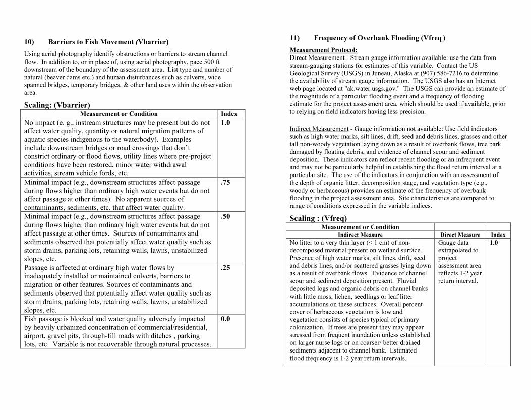
10) Barriers to Fish Movement (Vbarrier) Using aerial photography identify obstructions or barriers to stream channel flow. In addition to, or in place of, using aerial photography, pace 500 ft downstream of the boundary of the assessment area. List type and number of natural (beaver dams etc.) and human disturbances such as culverts, wide spanned bridges, temporary bridges, & other land uses within the observation area.

Scaling: (Vbarrier) Measurement or Condition Index

No impact (e. g., instream structures may be present but do not affect water quality, quantity or natural migration patterns of aquatic species indigenous to the waterbody). Examples include downstream bridges or road crossings that don’t constrict ordinary or flood flows, utility lines where pre-project conditions have been restored, minor water withdrawal activities, stream vehicle fords, etc.

1.0

Minimal impact (e.g., downstream structures affect passage during flows higher than ordinary high water events but do not affect passage at other times). No apparent sources of contaminants, sediments, etc. that affect water quality.

.75

Minimal impact (e.g., downstream structures affect passage during flows higher than ordinary high water events but do not affect passage at other times. Sources of contaminants and sediments observed that potentially affect water quality such as storm drains, parking lots, retaining walls, lawns, unstabilized slopes, etc.

.50

Passage is affected at ordinary high water flows by inadequately installed or maintained culverts, barriers to migration or other features. Sources of contaminants and sediments observed that potentially affect water quality such as storm drains, parking lots, retaining walls, lawns, unstabilized slopes, etc.

.25

Fish passage is blocked and water quality adversely impacted by heavily urbanized concentration of commercial/residential, airport, gravel pits, through-fill roads with ditches , parking lots, etc. Variable is not recoverable through natural processes.

0.0

11) Frequency of Overbank Flooding (Vfreq ) Measurement Protocol: Direct Measurement - Stream gauge information available: use the data from stream-gauging stations for estimates of this variable. Contact the US Geological Survey (USGS) in Juneau, Alaska at (907) 586-7216 to determine the availability of stream gauge information. The USGS also has an Internet web page located at "ak.water.usgs.gov." The USGS can provide an estimate of the magnitude of a particular flooding event and a frequency of flooding estimate for the project assessment area, which should be used if available, prior to relying on field indicators having less precision. Indirect Measurement - Gauge information not available: Use field indicators such as high water marks, silt lines, drift, seed and debris lines, grasses and other tall non-woody vegetation laying down as a result of overbank flows, tree bark damaged by floating debris, and evidence of channel scour and sediment deposition. These indicators can reflect recent flooding or an infrequent event and may not be particularly helpful in establishing the flood return interval at a particular site. The use of the indicators in conjunction with an assessment of the depth of organic litter, decomposition stage, and vegetation type (e.g., woody or herbaceous) provides an estimate of the frequency of overbank flooding in the project assessment area. Site characteristics are compared to range of conditions expressed in the variable indices.

Scaling : (Vfreq) Measurement or Condition

Indirect Measure Direct Measure Index No litter to a very thin layer (< 1 cm) of non-decomposed material present on wetland surface. Presence of high water marks, silt lines, drift, seed and debris lines, and/or scattered grasses lying down as a result of overbank flows. Evidence of channel scour and sediment deposition present. Fluvial deposited logs and organic debris on channel banks with little moss, lichen, seedlings or leaf litter accumulations on these surfaces. Overall percent cover of herbaceous vegetation is low and vegetation consists of species typical of primary colonization. If trees are present they may appear stressed from frequent inundation unless established on larger nurse logs or on coarser/ better drained sediments adjacent to channel bank. Estimated flood frequency is 1-2 year return intervals.

Gauge data extrapolated to project assessment area reflects 1-2 year return interval.

1.0

Measurement or Condition Indirect Measure Direct Measure Index

Thin litter cover (1-3 cm) ranging from recent to partly or completely decomposed material. Fluvial deposited logs and organic debris on channel banks with moss, lichen, seedlings, or decomposing leaf litter accumulations on these surfaces. Natural levees present immediately adjacent to the channel bank. Mature trees present along with some species typical of primary colonization. Bark of trees may show indications of damage from floating debris, and red squirrel midden accumulations may be concentrated at base of larger trees in the wetland. Estimated flood frequency is 2-10 year return intervals.


0.75

Thin litter cover (1-3 cm) ranging from recent to partly or completely decomposed material. Fluvial deposited logs and organic debris on channel banks with moss, lichen, seedlings, or decomposing leaf litter accumulations these surfaces. Natural levees present immediately adjacent to the channel bank. Mature trees present along with some species typical of primary colonization. Bark of trees may show indications of damage from floating debris, and red squirrel midden accumulations may be concentrated at base of larger trees in the wetland. Estimated flood frequency is 2-10 year return intervals.


0.50

Thick litter cover (>3 cm) with lower layer completely decomposed. No evidence of overbank deposits and fluvial transported debris not present. Dominant vegetation is mature trees (unless artificially manipulated - e.g., lawn or timber harvest). Estimated flood frequency is > 10 year return interval.

Gauge data extrapolated to project assessment area reflects > 10 year return interval.

0.5

Artificial flood control features that affect assessment area present (e.g. man-made levees, flood control channels, upstream flood control impoundments, etc.).

Gauge data extrapolated to project assessment area indicates that no overbank flooding is likely.

0.0

12) Flood Prone Area Storage Volume (Vstore) Identification and bounding of the flood prone area are key measurements because they establish the boundary of the assessment area and riverine wetland subclass. 1. Use either of the methods below to determine riverine boundary.

A) Visual Estimate: Estimate the width of the flood prone area visually. A crude estimate can be made using aerial photos or topographic maps. This should be done only if you have experience in the area. OR B) Direct Measurement: The flood prone area can be defined by the projection of a plane at twice the bankfull thalweg depth (deepest part of the stream, see the table and diagram on Riverine Wetland Terminology).

i. Determine the width of the channel by using a measuring tape and measuring from the edge of bankfull on one side of the stream to the bankfull on the opposite side of the stream.

ii. Determine the point on the stream channel transect at the deepest point of the stream. Measure the depth from the transect line.

iii. The flood prone area is defined by the projection of a plane at twice the bankfull thalweg depth. (See fig. 2).

2. Calculate a ratio by dividing the flood prone area width by the channel

width.

3. Based on the estimates above, scale the variable using the scaling index below.

Scaling: (Vstore) Direct measurements Index

Ratio > 2.5 1.0 Ratio 1.3 to 2.5 .50 Ratio 1.0 to 1.3 .10

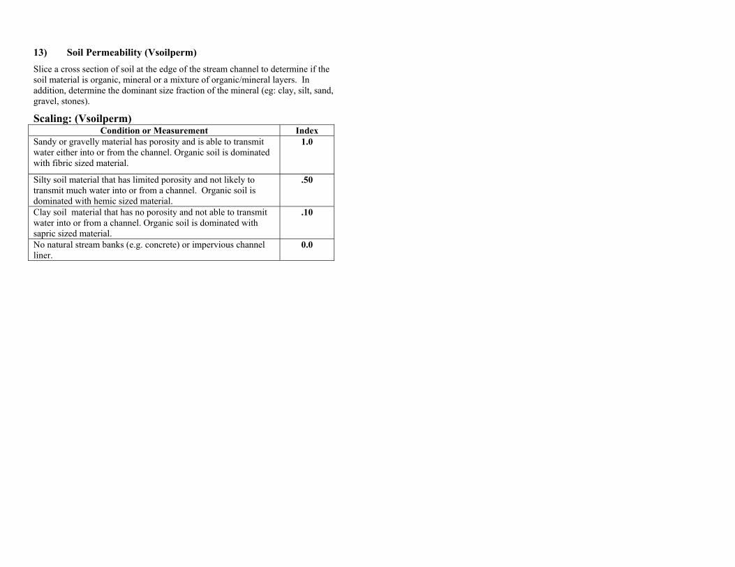
13) Soil Permeability (Vsoilperm) Slice a cross section of soil at the edge of the stream channel to determine if the soil material is organic, mineral or a mixture of organic/mineral layers. In addition, determine the dominant size fraction of the mineral (eg: clay, silt, sand, gravel, stones).

Scaling: (Vsoilperm) Condition or Measurement Index

Sandy or gravelly material has porosity and is able to transmit water either into or from the channel. Organic soil is dominated with fibric sized material.

1.0

Silty soil material that has limited porosity and not likely to transmit much water into or from a channel. Organic soil is dominated with hemic sized material.

.50

Clay soil material that has no porosity and not able to transmit water into or from a channel. Organic soil is dominated with sapric sized material.

.10

No natural stream banks (e.g. concrete) or impervious channel liner.

0.0

Riverine Wetlands: Vegetation and Land use

14) Tree Basal Area (Vtreeba) 15) Total Vegetative Cover (Vvegcov) 16) Number of Vegetative Strata (Vstrata) 17) Land Use of the Project Assessment Area (Vwetuse) 18) Land Use of Watershed Land use (Vwatersheduse)

14) Tree Basal Area (Vtreeba) Establish a point center quarter (PCQ) at least 30 ft from bankfull in a representative area of the floodplain. Using a prism, angle gauge measurement or other comparable instrument, stand at the center of the PCQ and count the trees within a 1/10 acre plot. Multiply the number of trees falling within the range of the cruise angle by the Basal Area Factor (BAF) which is indicated on the prism or angle gauge value, to determine the sq ft/acre of each tree species. Repeat this procedure to take a second measurement at a location that is ecologically similar to the first. For example, if the first BAF is done in coniferous forest, the second one should also be done in coniferous forest and not in emergent vegetation or a large gap, etc. 1) Number of trees (each species) counted ____ X _____BAF value =

_____feet2/acre.

Scaling: (Vtreeba) Measurement or Condition Index

Forest not appreciably altered (i.e., not harvested within > 80 years. Stand basal areas may vary due to natural gap processes.

1.0

Greater evidence of human disturbance ( > 200 feet2/acre). .75 Basal areas range > 150 < 200 feet2/acre.

.50

Basal areas are <150 feet2/acre. Evidence of human activity (e.g. selective logging).

.25

No trees present and riparian forest has been clearcut or modified by human disturbance. Variable is recoverable and sustainable through natural processes under current conditions.

.10

No trees present and riparian forest has been clearcut or modified by human disturbance. Variable is neither recoverable nor sustainable through natural processes under current conditions.

.00

15) Total Vegetative Cover (Vvegcov) 1) Visually estimate the total percent canopy cover by adding each strata

(forested, scrub/shrub, herbaceous, and moss and lichen). within 0.1 acre using the PCQ method. For sites dominated by herbaceous vegetation and low shrub vegetation, a line intercept method is used for cover measurements.

Cover Class Midpoints are obtained from the following table:

Use the following tables to list the most common species and their estimated percent cover using the cover class midpoint.

Tree Species Cover Class

Midpoint

Total Cover

% Cover Midpoint <1 0.5 1-5 3

6-15 10.5 16-25 20.5 26-50 38 51-75 63

76-95 85.5 >95 98

Small Trees Strata (>3’ & <10’, single stem)

Species Cover Class

Midpoint

Total Cover

Shrubs Strata (multiple stems) and Seedlings (<3’, single stem)

Species Cover Class

Midpoint

Total Cover

Herbaceous Strata: Forbs, Graminoids, Ferns and Fern Allies

Species Cover Class

Midpoint

Total Cover

Mosses and Lichens Strata

Species Cover Class

Midpoint

Total Cover 1. Total percent cover of Moss / Lichen Strata 2. Total percent cover of Herbaceous Strata 3. Total percent cover of Shrub Strata 4. Total percent cover of Tree Strata

Total Percent Vegetative Cover

Scaling: (Vvegcov) Condition Index

Greater than or equal to 120% total vegetative cover and site is not appreciably altered by human activity and dominated by native plant species.

1.0

Greater than or equal to 120% total vegetative and site has minimal disturbance by human activity and dominated by native plant species (i.e., foot trails, selective cutting ).

.75

> or equal to 120 % total vegetative and site significantly altered by human activity and dominated by native plant species (tree removal for ROW, heavy selective cutting).

.50

< or equal to 120 % total vegetative and site significantly altered by human activity. The variable is recoverable to reference standard conditions and sustainable through natural processes.

.10

< or equal to 120 % total vegetative and site is not recoverable to reference standard conditions nor sustainable through natural processes.

.00

16) Number of Vegetative Strata (Vstrata) Determine the number of strata that have a total cover of >10 %

Scaling: (Vstrata) Condition Index

Three or more forest strata present and dominated by native plant species.

1.0

Three or more forest strata present and dominated by native plant species (i.e. foot trails, selective cutting).

.75

Two or three forest strata present and dominated by native plant species (tree removal for ROW).

.50

One forest strata present and may include native and non-native plants.

.25

Site historically forested but no forest strata present and site significantly altered by human activity. The variable is recoverable to reference standard conditions and sustainable through natural processes.

.10

Site historically forested but no forest strata present and site significantly altered by human activity. The variable is neither recoverable to reference standard conditions or sustainable through natural processes.

.00

Riverine Land Use Assessment Review of land use is done in the field and with aerial photographs if available. Aerial photographs of the assessment and watershed provide more accurate and efficient evaluation of the land use variables. It is recommended that the aerial photographs be at a scale between 1:12,000 and 1:40,000. When using aerial photographs, obtain or produce a clear template showing a 1,000-foot radius for the photo scale used.

Impacts to the assessment area are described as a 900 arc (measured using a compass) looking upstream from the downstream edge of the project assessment area. The center of the axis of the 900 arc is the fall line (most direct line of water flow). Visually mark the boundaries of the arc using reference marks such as trees, buildings or flagging.

Within the 900 arc described above, angles of disturbance are measured by siting the arc distance of each disturbance (see diagram below). Measurements of

disturbance should be made to the edge of the contributing area or to 1000 feet, which ever is less. The angle of all disturbances are individually measured and categorized (see Table 18). In the example below, urban development has an

arc distance of 150. The remaining portion of the disturbance arc is undisturbed.

If multiple disturbances occur within the same arc, disturbances with the highest ranking (see the table below) take precedence over lower ranking disturbances that occur upslope. The lower ranking impacts are not considered in this case. Lower ranking impacts are measured if they occur down slope of higher-ranking impacts.

Within the arc of source described above, angles of disturbance are measured by siting the arc distance of each disturbance. Below is an example.

The following table shows the four-land use types used in the assessment area and the multiplier applied to each type. Land Use Categories Undisturbed: No significant human induced perturbation, except for natural or controlled burns. Recreation/Historic Forestry: Clearing of vegetation, clearing for right of ways, logging with temporary roads (no fill), pasture, and croplands. Rural: Low density housing (>5 acre lots), through-fill roads without ditches, forestry main haul roads (with through-fill and some ditches). Urban/Recent Forestry: Medium to high-density residential (<5 acre lots),

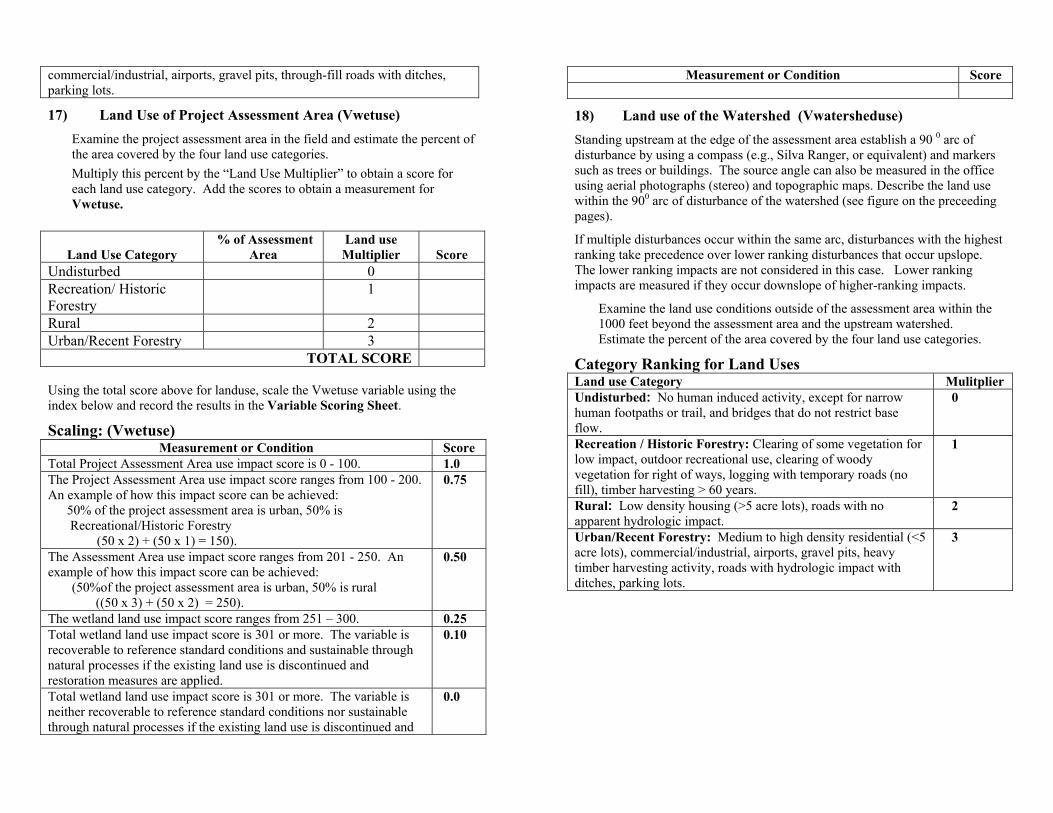
commercial/industrial, airports, gravel pits, through-fill roads with ditches, parking lots.

17) Land Use of Project Assessment Area (Vwetuse) Examine the project assessment area in the field and estimate the percent of

the area covered by the four land use categories. Multiply this percent by the “Land Use Multiplier” to obtain a score for

each land use category. Add the scores to obtain a measurement for Vwetuse.

Land Use Category % of Assessment

Area Land use Multiplier Score

Undisturbed 0 Recreation/ Historic Forestry

1

Rural 2 Urban/Recent Forestry 3

TOTAL SCORE Using the total score above for landuse, scale the Vwetuse variable using the index below and record the results in the Variable Scoring Sheet.

Scaling: (Vwetuse) Measurement or Condition Score

Total Project Assessment Area use impact score is 0 - 100. 1.0 The Project Assessment Area use impact score ranges from 100 - 200. An example of how this impact score can be achieved:

50% of the project assessment area is urban, 50% is Recreational/Historic Forestry

(50 x 2) + (50 x 1) = 150).

0.75

The Assessment Area use impact score ranges from 201 - 250. An example of how this impact score can be achieved: (50%of the project assessment area is urban, 50% is rural

((50 x 3) + (50 x 2) = 250).

0.50

The wetland land use impact score ranges from 251 – 300. 0.25 Total wetland land use impact score is 301 or more. The variable is recoverable to reference standard conditions and sustainable through natural processes if the existing land use is discontinued and restoration measures are applied.

0.10

Total wetland land use impact score is 301 or more. The variable is neither recoverable to reference standard conditions nor sustainable through natural processes if the existing land use is discontinued and

0.0

Measurement or Condition Score

18) Land use of the Watershed (Vwatersheduse) Standing upstream at the edge of the assessment area establish a 90 0 arc of disturbance by using a compass (e.g., Silva Ranger, or equivalent) and markers such as trees or buildings. The source angle can also be measured in the office using aerial photographs (stereo) and topographic maps. Describe the land use within the 900 arc of disturbance of the watershed (see figure on the preceeding pages). If multiple disturbances occur within the same arc, disturbances with the highest ranking take precedence over lower ranking disturbances that occur upslope. The lower ranking impacts are not considered in this case. Lower ranking impacts are measured if they occur downslope of higher-ranking impacts.

Examine the land use conditions outside of the assessment area within the 1000 feet beyond the assessment area and the upstream watershed. Estimate the percent of the area covered by the four land use categories.

Category Ranking for Land Uses Land use Category Mulitplier Undisturbed: No human induced activity, except for narrow human footpaths or trail, and bridges that do not restrict base flow.

0

Recreation / Historic Forestry: Clearing of some vegetation for low impact, outdoor recreational use, clearing of woody vegetation for right of ways, logging with temporary roads (no fill), timber harvesting > 60 years.

1

Rural: Low density housing (>5 acre lots), roads with no apparent hydrologic impact.

2

Urban/Recent Forestry: Medium to high density residential (<5 acre lots), commercial/industrial, airports, gravel pits, heavy timber harvesting activity, roads with hydrologic impact with ditches, parking lots.

3

Multiply this percent by the “Land Use Multiplier” to obtain a score for each land use category using the chart below. Add the scores to obtain a measurement for Vwatersheduse.

Land Use Category % of 900 arc of Disturbance

Land use Multiplier Score

Undisturbed 0 Recreation/Historic Forestry 1 Rural 2 Urban/Recent Forestry 3

TOTAL SCORE

Using the total score above for land use, scale the Vwetuse variable using the index below and record the results in the Variable Scoring Sheet.

Scaling: (Vwatersheduse) Measurement or Condition Index

Total Project Assessment Area use impact score is 0 – 100. 1.0 The Project Assessment Area use impact score ranges from 101-250. An example of how this impact score can be achieved: 50% of the project assessment area is urban , 50% is

Recreational/Historic Forestry (50 x 2 + 50 x 1 = 150).

0.75

The Assessment Area use impact score ranges from 251-400. An example of how this impact score can be achieved: 50%of the project assessment area is urban,

50% is rural ((50 x 3) + (50 x 2) = 250).

0.50

The wetland land use impact score ranges from 401 – 500. 0.25 Total wetland land use impact score is > 500. The variable is recoverable to reference standard conditions and sustainable through natural processes if the existing land use is discontinued and restoration measures are applied.

0.10

Total wetland land use impact score is > 500. The variable is neither recoverable to reference standard conditions nor sustainable through natural processes if the existing land use is discontinued and restoration measures are applied.

0.0

Step 4 (b) Summary of Slope River Proximal Variables

Slope River Proximal Wetlands HGM Rapid Assessment Field Process

Soils, Hydrology & Land Use

1 Vredox Dig a soil pit and examine for redox features

2 Vacro Determine thickness of acrotelm layer

3 Vsoilperm Determine dominant soil characteristics

4 Vsource Determine impact to upslope water source

5 Vsubout Look for indicators of seeps

6 Vfreq Look for indicators of high water marks

7 Vstore Determine if there are direct & indirect indicators of water storage areas

8 Vwetuse Determine land use in project assessment area

9 Vadjuse Determine land use in adjacent area

Microtopography 10 Vmicro Measure microtopography

11 Vsurwat Measure water storage

Vegetation and Coarse Wood 12 Vvegcov Estimate the total % of vegetative cover

13 Vstrata Count the number of vegetative strata

14 Vgaps Count the number of gaps in the veg. canopy

15 Vtreeba Measure tree basal area

16 Vdecomp Count the number of logs in different stages of decomposition

17 Vcwd

Count the number of coarse wood pieces

HGM Asessment Area: Slope River Proximal Wetlands

Water Flow 1000 ft Fall Line Project

Assessment Area 500 ft (adjuse)

Flags 50.0 ft from center

90% Arc of Disturbance

Stream Channel

Flags 37.5’ , 0.10 acre PCQ

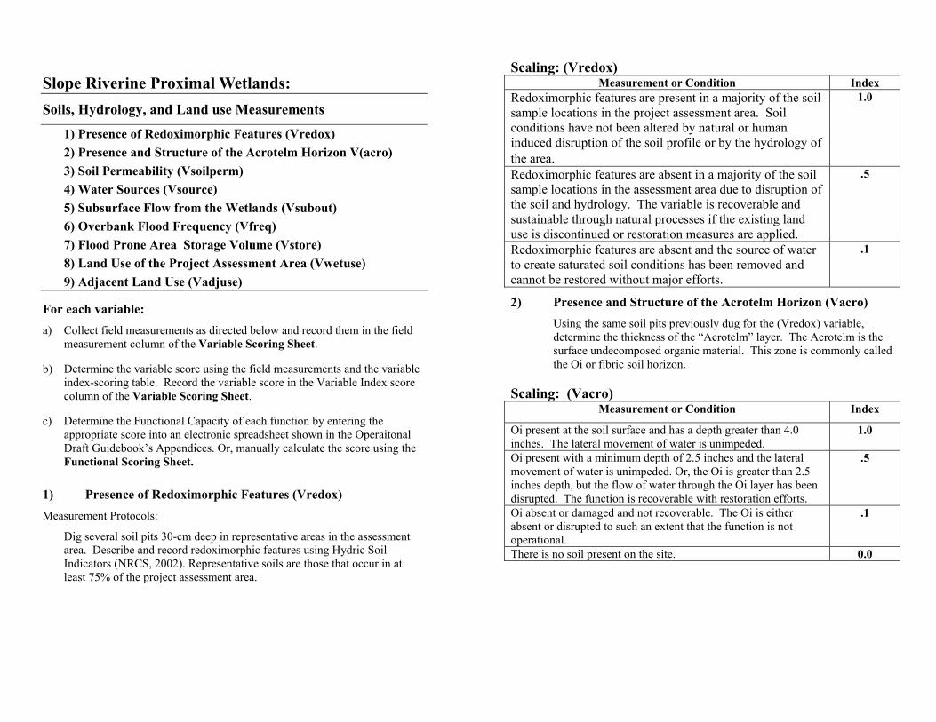
Slope Riverine Proximal Wetlands: Soils, Hydrology, and Land use Measurements

1) Presence of Redoximorphic Features (Vredox) 2) Presence and Structure of the Acrotelm Horizon V(acro) 3) Soil Permeability (Vsoilperm) 4) Water Sources (Vsource) 5) Subsurface Flow from the Wetlands (Vsubout) 6) Overbank Flood Frequency (Vfreq) 7) Flood Prone Area Storage Volume (Vstore) 8) Land Use of the Project Assessment Area (Vwetuse) 9) Adjacent Land Use (Vadjuse)

For each variable: a) Collect field measurements as directed below and record them in the field

measurement column of the Variable Scoring Sheet.

b) Determine the variable score using the field measurements and the variable index-scoring table. Record the variable score in the Variable Index score column of the Variable Scoring Sheet.

c) Determine the Functional Capacity of each function by entering the appropriate score into an electronic spreadsheet shown in the Operaitonal Draft Guidebook’s Appendices. Or, manually calculate the score using the Functional Scoring Sheet.

1) Presence of Redoximorphic Features (Vredox) Measurement Protocols:

Dig several soil pits 30-cm deep in representative areas in the assessment area. Describe and record redoximorphic features using Hydric Soil Indicators (NRCS, 2002). Representative soils are those that occur in at least 75% of the project assessment area.

Scaling: (Vredox) Measurement or Condition Index

Redoximorphic features are present in a majority of the soil sample locations in the project assessment area. Soil conditions have not been altered by natural or human induced disruption of the soil profile or by the hydrology of the area.

1.0

Redoximorphic features are absent in a majority of the soil sample locations in the assessment area due to disruption of the soil and hydrology. The variable is recoverable and sustainable through natural processes if the existing land use is discontinued or restoration measures are applied.

.5

Redoximorphic features are absent and the source of water to create saturated soil conditions has been removed and cannot be restored without major efforts.

.1

2) Presence and Structure of the Acrotelm Horizon (Vacro) Using the same soil pits previously dug for the (Vredox) variable, determine the thickness of the “Acrotelm” layer. The Acrotelm is the surface undecomposed organic material. This zone is commonly called the Oi or fibric soil horizon.

Scaling: (Vacro) Measurement or Condition Index

Oi present at the soil surface and has a depth greater than 4.0 inches. The lateral movement of water is unimpeded.

1.0

Oi present with a minimum depth of 2.5 inches and the lateral movement of water is unimpeded. Or, the Oi is greater than 2.5 inches depth, but the flow of water through the Oi layer has been disrupted. The function is recoverable with restoration efforts.

.5

Oi absent or damaged and not recoverable. The Oi is either absent or disrupted to such an extent that the function is not operational.

.1

There is no soil present on the site. 0.0

3) Soil Permeability (Vsoilperm) Dig a soil pit from bankfull depth to channel bed and determine if the soil

material is organic, mineral or a mixture of organic/mineral layers. Determine the dominant size fraction of the mineral (eg: clay, silt, sand,

gravel, stones).

Scaling: (Vsoilperm) Condition or Measurement Index

Sandy or gravelly material that has high porosity and is able to transmit water either into or from the channel. Organic soil is dominated with fibric sized material.

1.0

Silty soil material that has limited porosity and not likely to transmit much water into or from the channel. Organic soil is dominated with hemic sized material.

.5

Clay soil material that has no porosity and not able to transmit water into or from a channel. Organic soil is dominated with sapric sized material.

.1

No natural stream banks (eg: concrete) or impervious channel liner.

0

4) Water Sources (Vsource) Definition: Vsource is the condition of the contributing area for water (i.e., surface and shallow subsurface waterflow) upslope of the assessment area within a 900 arc. 1) Looking upslope from the center of the assessment area, project a 900 arc using reference points such as trees or buildings. 2) Within the 900 arc, measure the extent of each disturbance as a fraction of the arc in degrees. The angle of all disturbances are individually measured and categorized (see “Category Ranking for disturbance table below). If multiple disturbances occur within the same arc, measure the disturbance with the highest ranking (see the table below) and all other disturbances between that point and the assessment area. The following calculations should then be made: 3) Sum all segments of disturbance arc length that fall into the same category of disturbance (See the following “Category Ranking for Perturbations” table). Express as a percent of total source arc length. 4) Multiply the total arc length for each category by the category rank (provided in the following tables) to achieve a weighted arc length. Add all weighted arc length percentages to get the hydrologic source impact score.

The following table shows the four land use types used in the assessment and the multiplier applied to each type.

Land Uses and Multiplier Undisturbed: No significant human induced disturbance. 0 Recreation/Historic Forestry: Clearing of vegetation, clearing for right of ways, logging with temporary roads (no fill), pasture and croplands.

1

Rural: Low density housing (>5 acre lots), through-fill roads without ditches, forestry main haul roads (with through-fill and some ditches).

3

Urban/Recent Forestry: Medium to high-density residential (<5 acre lots), commercial/industrial, airports, gravel pits, through-fill roads with ditches, parking lots.

4

Scaling: (Vsource) Measurement or Condition Score

Hydrologic source impact scores range from 0 to 180. 1.0

Hydrologic source impact scores range from > 180 to 360. 0.75



Hydrologic source impact scores range from >720 and the variable is recoverable.

Hydrologic source impact score is >720 and the variable is not recoverable (e.g., parking lot, fill pad, paved road).

0.0

5) Subsurface Flow From the Wetlands (Vsubout) Determine presence of seeps, springs, etc. that occur at and downslope of the interface between the riverine and slope wetland. Ice bulges during very cold seasons can be used as a visual indication of this variable.

Scaling: (Vsubout) Measurement or Condition Index

Areas upslope of the riverine/slope interface within the assessment area are predominantly undisturbed, native soils, and plant communities AND direct evidence of subsurface flow is observed along the interface (e.g., seeps, upwellings, iron-floc discharge points, etc.).

1.0

Areas upslope of the riverine/slope interface within the assessment area are predominantly undisturbed, native soils, and plant

0.5

communities AND no direct evidence of subsurface flow along the interface is observed. OR Areas upslope of the riverine/slope interface within the assessment area are predominantly disturbed soils and/or plant communities AND direct evidence of subsurface flow along the interface is observed. Areas upslope of the riverine/slope interface within the assessment area are predominantly hard surfaces or fill AND direct evidence of subsurface flow along the interface is observed.

0.25

Areas upslope of the riverine/slope interface are predominantly hard surfaces or fill AND no direct evidence of subsurface flow along the interface is observed.

0.0

6) Overbank Flood Frequency (Vfreq) Follow the protocol below depending upon whether stream gauge information is available or not.

(a) Stream gauge information available - Data from stream-gauging stations are reliable estimates of this variable. Contact the US Geological Survey (USGS) in Juneau, Alaska at (907) 586-7216 to determine the availability of stream gauge information. The USGS also has an Internet web page located at "ak.water.usgs.gov." The USGS can provide an estimate of the magnitude of a particular flooding event and a frequency of flooding estimate for the project assessment area, which should be used if available, prior to relying on visual field indicators having less precision.

(b) Gauge information not available - Other field indicators include high water marks, silt lines, drift, seed and debris lines, grasses and other tall non-woody vegetation laying down as a result of overbank flows, tree bark damaged by floating debris, and evidence of channel scour and sediment deposition. These indicators can reflect recent flooding or an infrequent event and may not be particularly helpful in establishing the flood return interval at a particular site. However, the use of the indicators in conjunction with an assessment of the depth of organic litter, decomposition stage, and vegetation type (e.g., woody or herbaceous) provides an estimate of the frequency of overbank flooding in the project assessment area. Site characteristics are compared to range of conditions expressed in the variable indexes.

Scaling: (Vfreq)

Indirect Measure Direct Measure Index

No litter to a very thin layer (< 1 cm) of non-decomposed material present on wetland surface. Presence of high water marks, silt lines, drift, seed and debris lines, and/or scattered grasses lying down as a result of overbank flows. Evidence of channel scour and sediment deposition present. Fluvial deposited logs and organic debris on channel banks with little moss, lichen, seedlings or leaf litter accumulations on these surfaces. Overall percent cover of herbaceous vegetation is low and vegetation consists of species typical of primary colonization. If trees are present they may appear stressed from frequent inundation unless established on larger nurse logs or on coarser/ better drained sediments adjacent to channel bank. Estimated flood frequency is 1-2 year return intervals.


1.0

Thin litter cover (1-3 cm) ranging from recent to partly or completely decomposed material. Fluvial deposited logs and organic debris on channel banks with moss, lichen, seedlings, or decomposing leaf litter accumulations on these surfaces. Natural levees present immediately adjacent to the channel bank. Mature trees present along banks with some species typical of primary colonization. Bark of trees may show indications of damage from floating debris, and red squirrel midden accumulations may be concentrated at base of larger trees in the wetland. Estimated flood frequency is 2-10 year return intervals.


0.75

Thick litter cover (>3 cm) with lower layer completely decomposed. No evidence of overbank deposits and fluvial transported debris not present. Dominant vegetation is mature trees (unless artificially manipulated - e.g., lawn or timber harvest). Estimated flood frequency is > 10 year return interval

Gauge data extrapolated to project assessment area reflects > 10 year return interval.

0.5

Indirect Measure Direct Measure Index

Artificial flood control features that affect assessment area present (e.g., man-made levees, flood control channels, upstream flood control impoundments, etc.).

Gauge data extrapolated to project assessment area indicates that no overbank flooding is likely.

0.0

7) Flood Prone Area Storage Volume (Vstore) Definition: Ratio of flood prone area width divided by channel width at bankfull. Use either of the methods below to determine riverine boundary.

A) Visual Estimate: Estimate the width of the flood prone area visually. A crude estimate can be made using aerial photos or topographic maps. This should be done only if you have experience in the area. OR B) Direct Measurement: The flood prone area can be defined by the projection of a plane at twice the bankfull thalweg depth (deepest part of the stream).

1) Determine the width of the channel by using a measuring tape and measuring from the edge of bankfull on one side of the stream to the bankfull on the opposite side of the stream.

2) Determine the point on the stream channel transect at the deepest point of the stream. Measure the depth from the transect line.

3) The flood prone area is defined by the projection of a plane at twice the bankfull thalweg depth.

4) Calculate a ratio by dividing the flood prone area width by the channel width.

5) Based on the estimates above, scale the variable using the scaling index below.

6) Calculate the ratio by dividing the flood prone area width by the channel width. Report the ratio as a unit less number.

Scaling: (Vstore) Direct measurements Index Ratio > 2.5 1.0 Ratio 1.3 to 2.5 .50 Ratio 1.0 to 1.3 .10

8) Land Use of the Project Assessment Area (Vwetuse) Estimate the percent of the project assessment area covered by the following land use categories:

Category Ranking for Observed Wetland Land Uses Undisturbed: No human induced disturbance, except for narrow footpaths, trails, and bridges that do not restrict base flow.

0

Recreation/Historic Forestry: Clearing of vegetation for low impact outdoor recreational use, clearing of woody vegetation for right of ways, logging with temporary roads (no fill), timber harvesting > 60 years.

1

Rural: Low density housing (>5 acre lots), roads with no apparent hydrologic impact.

2

Urban/Recent Forestry: Medium to high density residential (<5 acre lots), commercial/industrial, airports, gravel pits, heavy timber harvesting activity, roads with hydrologic impact with ditches, parking lots.

3

The following calculations should then be made: Multiply the percent for each land use category by the category rank

(provided in Table 10) to achieve a weighted score. Add all weighted scores to get the total for the Project Assessment Area use

impact score.

Land Use Category % area of Disturbance


Undisturbed 0 Recreation/Historic Forestry 1 Rural 2 Urban/Recent Forestry 3 TOTAL :

Using the total score below scale the variable using the index below.

Scaling: (Vwetuse) Measurement or Condition Index

Total Assessment Area use impact score is 0 – 100 1.0 The Assessment Area use impact score ranges from 100- 200. An example of how this impact score can be achieved:

(a) 50% of the project assessment area is urban , 50% is

0.75

Recreational/Historic Forestry (50 x 2) + (50 x 1) = 150). The Assessment Area use impact score ranges from 201 - 250. An example of how this impact score can be achieved: (a) 50% of the project assessment area is urban, 50% is rural ((50 x 3) + (50 x 2) = 250).

0.50

The wetland land use impact score ranges from 251 - 300. 0.25 Total wetland land use impact score is 301 or more. The variable is recoverable to reference standard conditions and sustainable through natural processes if the existing land use is discontinued and restoration measures are applied.

0.10

Total wetland land use impact score is 301 or more. The variable is neither recoverable to reference standard conditions nor sustainable through natural processes if the existing land use is discontinued and restoration measures are applied.

0.0

9) Adjacent Land Use (Vadjuse) Using visual observation, aerial photography, and other office or field resources and tools, follow these steps: Estimate an area 500 feet beyond the boundary of the upstream and

downstream side of the assessment area and determine the land use categories using the table below.

Facing upslope, estimate a 900 arc pointed upslope of the assessment area. Estimate the percent and type of disturbance within 1000 ft upslope staying within the 900 arc.

Estimate the percent of the area covered by the following land use categories below:

Category Ranking for Land Uses Undisturbed: No significant human induced disturbance, except for bridges that do not restrict base flow.

0

Recreation/Historic Forestry: Clearing of vegetation, clearing for right of ways, logging with temporary roads (no fill), pasture, and croplands.

1

Rural: Low density housing (>5 acre lots), through-fill roads without ditches, forestry main haul roads (with through-fill and some ditches).

2

Urban/Recent Forestry: Medium to high-density residential (<5 acre lots), commercial/industrial, airports, gravel pits, through-fill roads with ditches and parking lots.

3

The following calculations should then be made: Multiply the percent for each land use category by the category rank

(provided in Table 13) to achieve a weighted score.

Land Use Category

Disturbance Arc Length / 90 X 100 = % of arc length


Undisturbed 0 = Recreation/Historic Forestry 1 = Rural 2 = Urban/Recent Forestry 3 =

Total Score Add all weighted scores to get the total adjacent land use impact score and scale the variable using the scaling and index below and record your result in the Variable Scoring Sheet.

Scaling: (Vadjuse) Measurement or Condition Score

The adjacent land use impact score ranges from 0 – 100. 1.0 The adjacent land use impact score ranges from 101 - 250. 0.75 The adjacent land use impact score ranges from 251 - 400. 0.50 The adjacent land use impact score ranges from 401 - 500. 0.25 The adjacent land use impact score is > 500. The variable is recoverable to reference standard conditions and sustainable through natural processes, if the existing land use is discontinued and restoration measures are applied.

0.10

The adjacent land use impact score is > 500. The variable is neither recoverable to reference standard conditions nor sustainable through natural processes, if the existing land use is discontinued and restoration measures are applied.

0.0

River Proximal Slope Wetland Measurements for Microtopography

10) Microtopographic Features V(micro) 11) Presence of Surface Water Storage (Vsurwat) For each variable:

a) Collect field measurements as directed below and record them in the field measurement column of the Variable Scoring Sheet.


c) Determine the Functional Capacity of each function by entering the appropriate score into an electronic spreadsheet shown in the Operational Draft Guidebook’s Appendices. Or, manually calculate the score using the Functional Scoring Sheet.

Use a point-center quarter (PCQ) to measure the microtopographic and vegetation variables. Determine the fall line within the assessment area for forming the axis of a 4-quadrat PCQ sampling area. Flag 37.5 ft and 50 ft along the axes of the quadrants. One transect should be perpendicular and one parallel to the stream channel

Use the 50 ft flagging for the two 100 ft transects to measure Vmicro and Vsurwat. In a large parcel you may want to do more to repeat this procedure in another area within the assessment area.

10) Microtopographic Features V(micro) Identify the dominant microtopographic surface at 10 ft intervals along the PCQ axes (within three feet of either side of the transect). Record the presence or evidence of ponding and/or static surface water at the same time. The table below describes the microtopographic surfaces.

Definition of Microtopographic Features Planar Surface Feature Criteria

Plane Level or nearly level ground surface excluding level surfaces contained in channels, pits, or ponds.

Non–Planar Surface Features

Channel Linear feature formed by flowing water.

Pit Depression, hole, burrow. <50 square feet.

Pond Depression >50 square feet (e.g., flark in string bog).

Hummock Mound or raised surface (e.g., shrub dominated strang in string bog). These features usually have different vegetation than surrounding lower areas.

Tussock Surface formation developed from tufted plants such as cottongrass.

Coarse Wood Woody debris >2” diameter that is lying on the surface or is <45 degrees from vertical.

Root Mass Root system and soil uplifted from fallen trees.

Other Describe.

PCQ Perpendicular Transect 1 Feet

Data Point 1 2 3 4 5 6 7 8 9 10 Planar or Non-Planar (0=Planar; 1= Non-Planar)

Presence or Evidence of Ponding (0= no; 1= yes)

PCQ Parallel Transect 2 Feet

Data Point 1 2 3 4 5 6 7 8 9 10 Planar or Non- Planar (0=Planar; 1= Non-Planar)

Presence or Evidence of Ponding (0 = no; 1= yes)

Total number of non-planar surface features recorded on the 2 transect tables: ______. Divide the above number by 20 and multiply the result by 100 to obtain percent of the observed features that are non-planar:

(____ ÷ 20) x 100 = _____ %.

Scaling: (Vmicro) Measurement or Condition Index The project assessment area is characterized by complex microtopographic relief (e.g., 50->80% of observed features are non-planar) AND assessment area is predominantly undisturbed, native soils, and plant communities.

1.0

The project assessment area is characterized by moderately complex microtopographic relief (e.g., 25-50% of observed features are non-planar) AND assessment area is predominantly undisturbed, native soils, and plant communities.

0.75

The project assessment area is characterized by moderately complex microtopographic relief (e.g., 25-50% of observed features are non-planar) AND assessment area is predominantly disturbed, native soils, and/or plant communities.

0.50

The project assessment area is characterized by some microtopographic relief (e.g., 1-25% of observed features are non-planar) AND assessment area is predominantly disturbed or undisturbed, native soils, and/or plant communities.

0.25

Microtopographic features are absent. 0.0

11) Presence of Surface Water (Vsurwat) Determine the percent cover of ponds and other depressions that store water in the assessment area along the 100-ft transects completed for Vmicro. Total number of observations from the 2 transect tables where there was the

presence or evidence of ponding: _____. Divide this number by 20 and multiply the result by 100 to obtain percent of

the observation points where ponding occurs: (____ ÷ 20) x 100 = _____ %.

Scaling: (Vsurwat)

Measurement or Condition Index Observations or evidence of surface water or ponds in >50% or more of the assessment area, project assessment area is either predominantly undisturbed, soils, and native plant communities. OR Observations or evidence of surface water or ponds in >50% or more of the assessment area, minor anthropogenic modifications may be present but no substantial impact to site topography is apparent (e.g., vegetation clearing, footpaths, wooden walkways, etc.).

1.0

Observations or evidence of surface water or ponds in 10-50% of the assessment area; project assessment area is predominantly undisturbed soils and native plant communities. OR Observations or evidence of surface water or ponds in 10-50% of the assessment area, minor human disturbances or modifications may be present but no substantial impact to site topography is apparent (e.g., vegetation clearing, foot paths, wooden walkways, etc.).

.75

Observations or evidence of surface water or ponds in <10% of the assessment area, minor human disturbances or modifications may be present but no substantial impact to site topography is apparent (e.g., vegetation clearing, foot paths, wooden walkways, etc.).

.50

No observations or evidence of surface water or ponds within assessment area, project assessment area is predominantly undisturbed soils and native plant communities.

.25

No observations or evidence of surface water or ponds within assessment area, project assessment area is predominantly disturbed by human activities but recoverable through natural processes.

.10

No observations or evidence of surface water or ponds within assessment area, variable is not recoverable through natural processes.

.00

Slope River Proximal e Wetlands Measurements for Vegetation and Coarse Wood 12) Total Vegetative Cover (vegcov)

13) Number of Vegetative Strata (Vstrata)

14) Canopy Gaps (Vgaps)

15) Basal Area of Trees (Vtreeba)

16) Log Decomposition (Vdecomp)

17) Number of Coarse Wood (Vcwslope)

For each variable: a) Collect field measurements as directed below and record them in the

field measurement column of the Variable Scoring Sheet.


c) Determine the Functional Capacity of each function by entering the appropriate score into an electronic spreadsheet shown in the Operational Draft Guidebook’s Appendices. Or, manually calculate the score using the Functional Scoring Sheet.

Use the point center quarter (PCQ) method for the vegetation variables: vegetative cover (Vvegcov), vegetative strata (Vstrata), gaps in the canopy (Vgaps), basal area of trees (Vtreeba), logs in decomposition (Vdecomp), and number of coarse wood (Vcwslope).

12) Total Vegetative Cover (Vvegcov) 1) Visually estimate the total percent canopy cover by adding each strata




6-15 10.5 16-25 20.5 26-50 38 51-75 63 76-95 85.5 >95 98



Midpoint

Total Cover


Species Cover Class

Midpoint

Total Cover


Species Cover Class

Midpoint

Total Cover


Species Cover Class

Midpoint

Total Cover


Species Cover Class

Midpoint



Using the Total Sum vegetative Cover Scale (Vvegcov) below and record the results in the scoring sheets .

Scaling: (Vvegcov) Condition Index

Greater than or equal to 120% total vegetative cover and site is not appreciably altered by human activity and dominated by native plant species.

1.0

Greater than or equal to 120% total vegetative and site has minimal disturbance by human activity and dominated by native plant species (i.e., foot trails, selective cutting ).

.75

> or equal to 120 % total vegetative and site significantly altered by human activity and dominated by native plant species (tree removal for ROW, heavy selective cutting).

.50

< or equal to 120 % total vegetative and site significantly altered by human activity. The variable is recoverable to reference standard conditions and sustainable through natural processes.

.10

< or equal to 120 % total vegetative and site is not recoverable to reference standard conditions nor sustainable through natural processes.

.00

13) Number of Vegetative Strata (Vstrata) Determine the number of strata that have a total cover of >10 %

Scaling: (Vstrata) Condition Index

Three or more forest strata present and dominated by native plant species.

1.0

Three or more forest strata present and dominated by native plant species (i.e. foot trails, selective cutting).

.75

Two or three forest strata present and dominated by native plant species (tree removal for ROW).

.50

One forest strata present and may include native and non-native plants.

.25

Site historically forested but no forest strata present and site significantly altered by human activity. The variable is recoverable to reference standard conditions and sustainable through natural processes.

.10

Condition Index Site historically forested but no forest strata present and site significantly altered by human activity. The variable is neither recoverable to reference standard conditions or sustainable through natural processes.

.00

14) Canopy Gaps (Vgaps) Using a vertical sitting perspective (rather than oblique), estimate or

measure the abundance of canopy gaps (percent cover as projected to the forest floor) within the forest. Gaps may be measured directly (e.g., project the openings to the forest floor, define with flagging, and measure the footprint), or estimated. If estimated rather than measured, the field assessor may find that mentally moving the openings together to determine the gap percentage within the assessment area will improve precision. For large areas, this variable may be estimated using aerial photography.

Scaling: (Vgaps) Measurement Index

No human disturbance evident within Project Assessment Area however site may reflect minor to severe natural disturbance. Forest canopy can intercept a large portion of snowfall; arboreal lichens typically present. Gaps comprise approximately 25-35% of the forest canopy.

1.0

Canopy gaps comprise 25-35% of the Assessment Area. Anthropogenic disturbance may be present but is minor (i.e., individual tree selection, boardwalks or limited use recreational trails, isolated recreational cabins, small communication towers, etc.). Forest canopy is dense enough to intercept a large portion of snowfall; arboreal lichens typically present.

0.75

Forest has been logged >5 years ago, but is in early successional stage. Herbaceous and shrub vegetation established, some trees reaching mid-canopy levels.

0.50

Forest has been recently (within 5 years) clearcut or second growth is dense with canopy closed such that gaps comprise <5% of forest within Assessment Area. Recovery is possible through forestry management activities or natural processes. Forest floor composed primarily of logging debris or leaf litter with little herbaceous or shrub growth.

0.25

Recovery is not possible due to anthropogenic disturbance (i.e., site is paved and/or all vegetation is otherwise permanently removed).

0.0

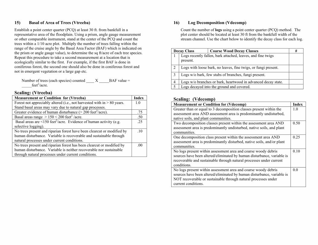
15) Basal of Area of Trees (Vtreeba) Establish a point center quarter (PCQ) at least 30 ft. from bankfull in a representative area of the floodplain. Using a prism, angle gauge measurement or other comparable instrument, stand at the center of the PCQ and count the trees within a 1/10 acre plot. Multiply the number of trees falling within the range of the cruise angle by the Basal Area Factor (BAF) which is indicated on the prism or angle gauge value), to determine the sq ft/acre of each tree species. Repeat this procedure to take a second measurement at a location that is ecologically similar to the first. For example, if the first BAF is done in coniferous forest, the second one should also be done in coniferous forest and not in emergent vegetation or a large gap etc.

Number of trees (each species) counted ____ X _____BAF value = _____feet2/acre.

Scaling: (Vtreeba) Measurement or Condition for (Vtreeba) Index Forest not appreciably altered (i.e., not harvested with in > 80 years. Stand basal areas may vary due to natural gap processes.

1.0

Greater evidence of human disturbance (> 200 feet2/acre). .75 Basal areas range > 150 < 200 feet2 /acre. .50 Basal areas are <150 feet2/acre. Evidence of human activity (e.g. selective logging).

.25

No trees present and riparian forest have been clearcut or modified by human disturbance. Variable is recoverable and sustainable through natural processes under current conditions.

.10

No trees present and riparian forest has been clearcut or modified by human disturbance. Variable is neither recoverable nor sustainable through natural processes under current conditions.

.00

16) Log Decomposition (Vdecomp) Count the number of logs using a point center quarter (PCQ) method. The

plot center should be located at least 30 ft from the bankfull width of the stream channel. Use the chart below to identify the decay class for each log.

Decay Class Coarse Wood Decay Classes # 1 Logs recently fallen, bark attached, leaves, and fine twigs

present.

2 Logs with loose bark, no leaves, fine twigs, or fungi present.

3 Logs w/o bark, few stubs of branches, fungi present.

4 Logs w/o branches or bark, heartwood in advanced decay state. 5 Logs decayed into the ground and covered.

Scaling: (Vdecomp) Measurement or Condition for (Vdecomp) Index Greater than or equal to 3 decomposition classes present within the assessment area AND assessment area is predominantly undisturbed, native soils, and plant communities.

1.0

Two decomposition classes present within the assessment area AND assessment area is predominantly undisturbed, native soils, and plant communities.

0.50

One decomposition class present within the assessment area AND assessment area is predominantly disturbed, native soils, and/or plant communities.

0.25

No logs present within assessment area and coarse woody debris sources have been altered/eliminated by human disturbance, variable is recoverable and sustainable through natural processes under current conditions.

0.10

No logs present within assessment area and coarse woody debris sources have been altered/eliminated by human disturbance, variable is NOT recoverable or sustainable through natural processes under current conditions.

0.0

17) Number of Coarse Wood (Vcwslope) Count the number of downed coarse wood using a point center quarter (PCQ) method. The plot center should be located at least 30ft from the bankfull width of the stream channel. In each quarter, record the distance from plot center to the middle of the nearest piece of downed coarse and dead wood ≥2” diameter. If a piece spans quarter boundaries (e.g., spans the NE - SE quarter boundary), it is counted only in the quarter that contains most of the piece. If a quarter does not contain coarse woody debris, the PCQ method cannot be used. In these cases, record the number of pieces of coarse down and dead wood within a 0.1-acre (0.04-ha) plot to calculate density. This method can also be used if there are a small number of pieces that can be easily counted. Densities on a per-acre basis are calculated from the plot data. Measure and record the distance to nearest piece of coarse woody debris in each quarter. Measure to the center of the piece.

NE Quadrant

SE Quadrant

SW Quadrant

NW Quadrant

Distance to nearest piece (feet)

Vcwslope Measurement

1. Total the distances recorded for the 4 quadrants. 2. Determine the average distance (total distance/4). 3. Square the average distance. 4. Divide 43,560 by the square of the average distance

CWD pieces/acre.

5. Record this result in the Indicator Measurement Result column in the Summary Table.

OR 1. If the PCQ method is not used, determine the CWD pieces/acre from

the pieces counted in a 0.1 - acre plot:

Cwslope pieces in 0.1 acre plot ______ x 10 = CWD pieces/acre

2. Record this result in the Indicator Measurement Result column in the Variable Scoring Sheet.

Scaling: (Vcwslope) Measurement or Condition Index Using the PCQ method, the average distance to the first piece of coarse wood is equal to or < 20 feet.

1.0

Using the PCQ method, the average distance to the first piece of coarse wood is > 20 feet and < 30 feet.

.75

> 30 feet and < 37.5 feet .50 No coarse wood found in the PCQ plot. The variable is recoverable to reference standard conditions and sustainable through natural processes.

.10

No coarse wood found in the PCQ plot. The variable is neither recoverable to reference standard conditions nor sustainable through natural processes.

.00

Point Center Quarter

Step 5a. Variable Scoring Sheet - Riverine

Variable Units of Measurement Field

Measurement

Variable Index Score

Vpebble-D50 Median size Vchanrough One Standard Deviation Vembedded % Embedded Pebbles Vcwpot Coarse Wood Potential

# of Pieces

Vcwin Coarse Wood in Channel

# of Pieces in Channel

Vlogjams Number of Logjams

# of Logjams

Vsubin Surface water into the A. Area

# of Features

Vshade Riparian Shade

% Riparian Shade

Valthydro Alteration of Hydroregime

Hydrologic Connections Disturbed

Vbarrier Downstream Barriers Vfreq # of Features Vstore # of Features Vsoilperm Soil Permeability

Soil Features

Vtreeba Tree Basal Area

Est. of Basal Area

Vvegcov Total Veg. Cover

Sum of % of Six (6)

Vstrata Vegetation Strata

# of Veg. Strata

Vwetuse Assessment Area Land use

% of Area Disturbed

Vwatersheduse Land use in Watershed

% of Area Disturbed

Step 5b. . Variable Scoring Sheet. – Slope River Proximal


Measurement Variable

Index Score Vredox Redoximorphic Features

Presence or Absence

Vacro Acrotelm Layer

Presence & Structure

Vsoilperm Soil Permeability

Condition of Soil

Vsource Water Source

% and Category of Observed Land Use

Vsubout Subsurface Water Flow Out

Evidence of Subsurface Flow

Vfreq Flood Frequency

Indicators of Frequent Flooding

Vstore Ratio of Flood Prone Area Vwetuse Assessment Area Land Use

Inches (cm)

Vadjuse Adjacent Land use

Degree of Slope

Vmicro Microtopography

Ratio of Observed Angle of Impacted Area

Vsurwat Surface water

Surface Water


# per Site


% Features, Presence of Ponding

Vgaps Canopy Gaps

Sum of % of Six (6) Vegetation Covers.

Vtreeba Basal Tree Area

% of Hydrologic Connections Disturbed

Vdecomp Log Decomposition


Vcwslope Coarse Wood

# of Pieces of Coarse Wood

Step 6a.. Functional Scoring Sheets - Riverine

Function Formulae

Functional Capacity

Index (FCI) 1) Channel meander Belt Integrity

= (Vwatersheduse + Vwetuse+ Valthydro + Vfreq + Vchanrough + Vcwpot + Vlogjam + Vcwin) / 8

2) Dynamic Flood Water Retention

= (Vstore + Vpebble-D50 + Vlogjam + Vcwin + Vvegcov) / 5 + Vwatersheduse + Vfreq) / 3

3) Nutrient Spiraling

= (Vsubin + Vcwin + Vcwpot + Vchanrough + Vsoilperm + Vwatersheduse + Vshade) / 7

4) Particulate Retention

= (Vcwin + Vcwpot + Vlogjams + Vtreeba + Vpebble-D50 + Vvegcov) / 6 + Vfreq) / 2

5) Removal of Imported Elements and Compounds

= (Valthydro + Vfreq + Vsubin + (Vvegcov + Vtreeba) / 2 + Vsoilperm) / 5

6) In-Channel Biota

= (Vshade + Vchanrough + Vembedded + Vwetuse + Vsubin) / 5

7) Coarse Wood = (Vcwin + Vlogjam + Vcwpot) / 3 + Vfreq) / 2

8) Riparian Vegetation

= (Vfreq + Vwetuse + Vwatersheduse + Vshade + (Vvegcov + Vstrata) / 2 + Vtreeba) / 6

9) Connectivity and Interspersion

= (Valthydro + Vsubin + Vwetuse + Vwatersheduse + Vbarrier) / 5

Step 6b.. Functional Scoring Sheet - Slope Riverine Proximal

Function Formulae

Functional Capacity

Index (FCI) 1) Dynamic Flood Water Retention Capacity

= (Vfreq + Vcwslope + Vsoilperm + Vmicro + Vvegcov +Vstore) / 6

2) Subsurface Water Retention Capacity

= (Vsource + (Vacro + Vsoilperm + Vdecomp)/ 3 + Vmicro + Vadjuse) / 4

3) Nutrient Cycling

= (Vadjuse + Vsurwat + Vvegcov + (Vsource + Vsubout) / 2 + (Vacro + Vredox + Vdecomp) / 3) / 5

4) Organic Carbon Export

= (Vsource + (Vacro + Vsoilperm + Vdecomp + Vredox + Vegcov) / 4+ Vsubout) / 3

5) Integrity of the Root Zone

= (Vsource +Vsurwat + Vacro + (Vredox + Vsoilperm) / 2) / 4

6) Maintenance of Wildlife Habitat Structure

= (Vvegcov + Vadjuse +Vwetuse + (Vsurwat + Vmicro) / 2 + Vstrata + (Vgaps + Vcwslope) 2) / 6

7) Maintenance of Plants

= (Vwetuse + Vvegcov + Vsource + Vtreeba + (Vsurwat + Vacro) / 2 + (Vredox + Vsoilperm) / 2) / 6

HGM Rapid Assessment Report Data Collection Sheets The following list and data collection sheets are necessary for completing an HGM Rapid Assessment Report

1) Step 1. Preliminary HGM Classification (Riverine) 2) Step 1 Preliminary HGM Classification (Slope River Proxi.) 3) Step 2. Site Information (completed in the office or field) 4) Step 3. Sketch a Map of Project Assessment Area. 5) Pebble Count & Embeddedness Work Sheet 6) Variable (15) Vegetative Cover (Vvegcov) worksheets. 7) Riverine Variable Scoring Sheet 8) Slope Variable Scoring Sheet 9) Riverine Functional Scoring Sheet 10) Slope Functional Scoring Sheet

(1) Step 1. Preliminary HGM Classification Identify, verify, and document the rationale used for recognizing HGM classes and subclasses within the project assessment area. Determine if the assessment area is a RIVERINE and/or SLOPE RIVER PROXIMAL Wetland Subclass by using the dominant characteristics outlined below. Show how the project assessment area satisfies a subclass definition provided in the guidebook by completing the form below. Specifically, include a discussion of the site characteristics and show how they are consistent with the dominant characteristics of the subclass.

Riverine Wetland Dominant Characteristics CHARACTERISTIC DESCRIPTION Hydrologic Source Unidirectional flow, higher order streams, derived

from non-glacial water sources

Vegetation Any vegetation life form (e.g., trees, shrubs, herbaceous, etc.) that are not in a marine, or estuarine system, nor directly influenced (i.e., actively flooded) by those systems.

Landforms Occur in valley bottoms, flow predominantly on bedrock, glacial till or glacial marine deposits. Low elevation stream reaches may flow on Pleistocene or Holocene alluvial gravel deposits, or deltaic estuarine deposits raised in elevation by tectonic lift.

Slope 0.001% to ≤ 2.2% Parent Materials Upper reaches: exposed bedrock, glacial till, and

colluvium over bedrock, alluvial sand, and gravel. Lower reaches: dense basal till, marine lucustrine and glacial fluvial sediments, and alluvial sand and gravel.



Hydrologic Source

Vegetation

Landform, soils

Slope

Slope River Proximal Wetland Dominant Characteristics CHARACTERISTIC DESCRIPTION

Location Located within 200 feet of the bankfull of a river channel.

Hydrologic Source Ground or surface water flow. Vegetation Any vegetation life form (e.g., trees, shrubs,

herbaceous, etc.) that are not in a marine, or estuarine system nor directly influenced (i.e., actively flooded) by those systems.

Landforms Occur adjacent to streams and valley sides. Occur in valley bottoms, flow predominantly on bedrock, glacial till or glacial marine deposits. Low elevation stream reaches may flow on Pleistocene or Holocene alluvial gravel deposits, or deltaic estuarine deposits raised in elevation by tectonic lift. Note: wetlands in closed depressions are out of the subclass.

Slope 0.1% to ≤25% Parent Materials Upper reaches: exposed bedrock, thin till, and

colluvium over bedrock. Lower reaches: dense basal till deposited by flowing glacial ice, outwash, gravel.



Hydrologic Source

Vegetation

Landform

Slope

Parent Materials

Soils

(3) Step 2. Site Information (Completed in the Field or Office)

Dates of Site Visit

Team Members

Field Notes/Observations

Collect and review information relevant to the site. This includes, but is not limited to: USGS, state, local, and other maps (at various scales) Geotechnical, soils, or environmental reports Correspondence, construction plans on the proposed project Published literature

Identify the documents that were collected and reviewed. Include a detailed description of each document (e.g., citation, date, scale, quadrangle name, etc.). If possible, attach copies of each document.

USGS, state, borough, and other maps (at various scales):

1. ______________________________________________

2. ______________________________________________

Air photos and other imagery: 1. ______________________________________________

2. ______________________________________________

Relevant geotechnical, soils, or environmental reports: 1. ______________________________________________

2. ______________________________________________

• Correspondence, construction plans, and specifications, etc. on the proposed project:

______________________________________________________

Relevant published literature: ______________________________________________________

Other documents:

Other Questions: Is a cataloged anadromous fish stream adjacent to or part of the assessment area?

Is the assessment area used by any federally listed threatened or endangered species?

Is the assessment area adjacent to a state listed impaired waterbody? Is the assessment area listed as a historic or cementary?

(4) Step 3. Sketch a map of Project Assessment Area

(5) 1) Median Pebble Size D50 (Vpebble-D50): Determine the median pebble size (D50) of the samples by using the Pebble Count Table following the procedure outline above.

Pebble Count & Embeddedness Work sheet

>2 2-4 5-8 9-16 17-32 33-64 65-128

129-256

257-512

512- 1024 > 1024

Embeddness Work Sheet

0 – 25% 26 – 50% 51 – 75% 76 – 100%

Image source, date, and scale: ____________________________

(6) 15) Total Vegetative Cover (Vvegcov) 1) Visually estimate the total percent canopy cover by adding each strata





Midpoint

Total Cover


Species Cover Class

Midpoint

Total Cover


Species Cover Class

Midpoint

Total Cover


Species Cover Class

Midpoint

Total Cover


6-15 10.5 16-25 20.5 26-50 38 51-75 63 76-95 85.5 >95 98


Species Cover Class

Midpoint



(7) Riverine Variables Scoring Sheet


Measurement

Variable Index Score

Vpebble-D50 Median size Vchanrough One Standard Deviation Vembedded % Embedded Pebbles Vcwpot Coarse Wood Potential

# of Pieces

Vcwin Coarse Wood in Channel

# of Pieces in Channel

Vlogjams Number of Logjams

# of Logjams

Vsubin Surface water into the A. Area

# of Features

Vshade Riparian Shade

% Riparian Shade

Valthydro Alteration of Hydroregime

Hydrologic Connections Disturbed

Vbarrier Downstream Barriers Vfreq # of Features Vstore # of Features Vsoilperm Soil Permeability

Soil Features

Vtreeba Tree Basal Area

Est. of Basal Area


Sum of % of Six (6)


# of Veg. Strata

Vwetuse Assessment Area Land use

% of Area Disturbed

Vwatersheduse Land use in Watershed

% of Area Disturbed

(8) Slope Riverine Proximal Variables Scoring Sheet


Measurement Variable

Index Score Vredox Redoximorphic Features

Presence or Absence

Vacro Acrotelm Layer

Presence & Structure

Vsoilperm Soil Permeability

Condition of Soil

Vsource Water Source


Vsubout Subsurface Water Flow Out

Evidence of Subsurface Flow

Vfreq Flood Frequency

Indicators of Frequent Flooding

Vstore Ratio of Flood Prone Area Vwetuse Assessment Area Land Use

Inches (cm)

Vadjuse Adjacent Land use

Degree of Slope

Vmicro Microtopography

Ratio of Observed Angle of Impacted Area

Vsurwat Surface water

Surface Water


# per Site


% Features, Presence of Ponding

Vgaps Canopy Gaps

Sum of % of Six (6) Vegetation Covers.

Vtreeba Basal Tree Area

% of Hydrologic Connections Disturbed

Vdecomp Log Decomposition


Vcwslope Coarse Wood

# of Pieces of Coarse Wood

(9) Riverine Functional Scoring Sheet

Function Formulae

Functional Capacity

Index (FCI) 1) Channel meander Belt Integrity

= (Vwatersheduse + Vwetuse+ Valthydro + Vfreq + Vchanrough + Vcwpot + Vlogjam + Vcwin) / 8

2) Dynamic Flood Water Retention

= (Vstore + Vpebble-D50 + Vlogjam + Vcwin + Vvegcov) / 5 + Vwatersheduse + Vfreq) / 3

3) Nutrient Spiraling

= (Vsubin + Vcwin + Vcwpot + Vchanrough + Vsoilperm + Vwatersheduse + Vshade) / 7

4) Particulate Retention

= (Vcwin + Vcwpot + Vlogjams + Vtreeba + Vpebble-D50 + Vvegcov) / 6 + Vfreq) / 2

5) Removal of Imported Elements and Compounds

= (Valthydro + Vfreq + Vsubin + (Vvegcov + Vtreeba) / 2 + Vsoilperm) / 5

6) In-Channel Biota

= (Vshade + Vchanrough + Vembedded + Vwetuse + Vsubin) / 5

7) Coarse Wood = (Vcwin + Vlogjam + Vcwpot) / 3 + Vfreq) / 2

8) Riparian Vegetation

= (Vfreq + Vwetuse + Vwatersheduse + Vshade + (Vvegcov + Vstrata) / 2 + Vtreeba) / 6

9) Connectivity and Interspersion

= (Valthydro + Vsubin + Vwetuse + Vwatersheduse + Vbarrier) / 5

(10) Slope Riverine Proximal Functional Scoring Sheet

Function Formulae

Functional Capacity

Index (FCI) 1) Dynamic Flood Water Retention Capacity

= (Vfreq + Vcwslope + Vsoilperm + Vmicro + Vvegcov +Vstore) / 6

2) Subsurface Water Retention Capacity

= (Vsource + (Vacro + Vsoilperm + Vdecomp)/ 3 + Vmicro + Vadjuse) / 4

3) Nutrient Cycling

= (Vadjuse + Vsurwat + Vvegcov + (Vsource + Vsubout) / 2 + (Vacro + Vredox + Vdecomp) / 3) / 5

4) Organic Carbon Export

= (Vsource + (Vacro + Vsoilperm + Vdecomp + Vredox + Vegcov) / 4+ Vsubout) / 3

5) Integrity of the Root Zone

= (Vsource +Vsurwat + Vacro + (Vredox + Vsoilperm) / 2) / 4

6) Maintenance of Wildlife Habitat Structure

= (Vvegcov + Vadjuse +Vwetuse + (Vsurwat + Vmicro) / 2 + Vstrata + (Vgaps + Vcwslope) 2) / 6

7) Maintenance of Plants

= (Vwetuse + Vvegcov + Vsource + Vtreeba + (Vsurwat + Vacro) / 2 + (Vredox + Vsoilperm) / 2) / 6

Field Guide and Data Collection Procedures...

Documents

Transcript of Field Guide and Data Collection Procedures...