1

Field Experiments in Developing Country Agriculture

Alain de Janvry*, Elisabeth Sadoulet*, and Tavneet Suri**1

July 2016

Abstract

This chapter provides a review of the role of field experiments in answering research questions in agriculture that ultimately let us better understand how policy can improve productivity and farmer welfare in developing economies. We first review recent field experiments in this area, highlighting the contributions experiments have already made to this area of research. We then outline areas where experiments can further fill existing gaps in our knowledge on agriculture and how future experiments can address the specific complexities in agriculture. Keywords: agriculture, field experiments, developing economies JEL Codes: Q1, 013, C93

* University of California at Berkeley. ** MIT Sloan School of Management. 1 We are grateful to Shweta Bhogale, Erin Kelley, Gregory Lane and Eleanor Wiseman for excellent research assistance, and to Mushfiq Mobarak, Abhijit Banerjee and Esther Duflo for their reviews of the paper and suggestions for improvements. We also benefited from the review materials on field experiments in agriculture prepared by Craig McIntosh, Rachel Glennerster, Christopher Udry, Ben Jaques-Leslie, and Ellie Porter. Errors and shortcomings are our own.

2

I. Introduction Agriculture is an important sector in most developing economies, often the main form of employment for a majority of individuals, and making up a substantial share of these economies’ GDP. For example, in 2014 for the low-income countries (as defined in the World Bank development indicators), agriculture made up 32% of GDP on average, declining to only 10% of GDP in 2014 in the middle-income countries. Similarly, in low-income countries, 70% of the population lives in rural areas, compared to 51% for middle-income countries. Agriculture may play a key role in the economic growth and industrialization of these economies, and potentially have impacts on poverty reduction, food security, environmental sustainability, and community development (World Bank, 2007). While there are remarkable success stories of agriculture playing a key transitional role, these are few and far between. This raises an important question for research: what can be done to help low-income countries use agriculture to its full potential in achieving development? A large research agenda to address this question has placed agriculture as one of the pillars of development economics, with chapters typically devoted to it in Handbooks of Development Economics and Agricultural Economics. However, many questions still remain unresolved due to the difficulties in establishing causality between determinants and outcomes in both positive and normative analyses. The use of field experiments (FE) offers an immense opportunity to address some of the outstanding issues in a rigorous and causal way. This chapter focuses on the role of FE in this area, briefly describing contributions that have already been made using FE, but also highlighting the specific complexities in the agricultural sector that such FE have had to deal with and that leave room for further experimental research in this area. We discuss six specific features of agricultural environments and farmer behavior that have implications for the design of FE and that illustrate the immense room for further contributions to better understand the questions posed above. They are: (1) the dependence of outcomes on random weather realizations and exposure to risk, (2) the spatial dimension of agriculture with corresponding high heterogeneity and transaction costs, (3) the existence of seasonality and long lags in production, (4) the prevalence of market failures and their implications for farm household decision-making, (5) the occurrence of local spillover effects, externalities, and general equilibrium effects, and (6) difficulties in measurement. For each of these features, we describe in detail the issues in agriculture and then how FE can be designed and implemented to close the remaining knowledge gaps in agriculture. This chapter is structured as follows. In Section II, we review the FE that have been used in agriculture in developing countries to provide a summary of the areas that that experiments have contributed to as well as to highlight the findings from these studies. In Section III, we provide a broad conceptual framework to better understand the role that field experiments can play in agriculture. In Section IV, we discuss each of the six areas where specific features of agriculture and the environment (both natural as well as economic) that farmers face have implications for the design and implementation of field experiments. In Section V, we conclude by summarizing potential new areas of research on agriculture that may benefit from the use of such experiments, including using FE to reveal the production function in agriculture. II. A Review of Field Experiments in Agriculture Over the last decade, there has been a rapid growth in the use of FE to study agricultural issues in development. Supporting the more general growth of FE in social science research, there has been a commitment from donors to better understand some of the outstanding questions in agriculture using this approach. A good example is the Agricultural Technology Adoption Initiative (ATAI) at the Abdul Latif Jameel Poverty Action Lab (J-PAL) and the Center for Effective Global Action (CEGA) that funds studies on the adoption and impact of technologies in agriculture. In the process to starting ATAI, a white paper was prepared on the then outstanding issues with technology adoption (Jack, 2011). Five years later, ATAI

3

alone has funded 42 different studies in Africa and South Asia, across a wide range of topic areas. The overwhelming majority of these studies have focused on the determinants of the modernization of agriculture and, in particular, the adoption, diffusion, and impact of technological and institutional innovations in agriculture. We summarize the experiments in agriculture by looking at the following topics: (1) the role of information about technologies in decision-making and how it affects farmer behavior, (2) the role of liquidity constraints and access to credit in technology adoption, and (3) the availability of financial products and technologies to reduce farmer exposure to risks and mitigate the impact of shocks on farmers welfare, (4) the estimation of price responses and the role of subsidies in agriculture, (5) the role of access to price information for farmers, (6) contracts in agricultural value chains and (7) the heterogeneity of conditions and types in influencing outcomes. 1. When does facilitating access to information about agricultural technologies to farmers make a

contribution to agricultural development, and what is the most cost effective way of doing this? Extension services or training are likely to be most useful when new knowledge, not directly accessible to farmers, is needed to adopt a technological or institutional innovation. Glennerster and Suri (2015) showed that training was instrumental in the profitability of NERICA, a new rice variety with specific cultivation practices. Farmers who received both NERICA and training increased yields by 16%, while those with NERICA and no training experienced a small decline in yields. Information provided by extension agents can, however, be misleading to farmers if these agents pursue a different objective function than that of farmers (typically maximizing yields instead of profit or utility) or do not properly account for the opportunity cost of farmers’ labor time (for example in recommending the adoption of the highly labor intensive System of Rice Intensification (SRI) or the use of Conservation Agriculture (CA) without chemical herbicides). Duflo et al. (2008) thus found that properly timed and dosed fertilizers can be profitable in Kenya, but that they were not profitable if used according in the dosages recommended by the Ministry of Agriculture. Similarly, farmers may fail to use available information, thus leaving money on the table. For example, studying seaweed farmers in Indonesia, Hanna et al. (2014) showed that farmers may be far from the efficiency frontier simply because they “fail to notice” some important aspects of the information they possess, such as the role of pod size as opposed to simply pod spacing on seaweeds. Information can also be conveyed through social networks (Foster and Rosenzweig, 1995), though social learning may be limited by heterogeneity of farmer conditions and types. Beaman et al. (2014) analyze the factors that favor the adoption of pit planting in Malawi, a water harvesting technique commonly used in West Africa but largely unknown in Southern Africa. They found that social networks are useful to convey information, but that they are most effective when information is confirmed by more than one source. This suggests the need for several “seed” farmers for effective diffusion when introducing information on an innovation in a social network with heterogeneity of conditions and types. Cai et al. (2015) randomized the training about a new weather insurance product in China. They found that social networks are effective at transmitting knowledge acquired by those who participated in intensive training sessions, but not at sharing information about adoption decisions taken by particular individuals that is kept private. This suggests that information about individual decisions on the adoption of subsidized innovations, which is quite helpful for others to decide to adopt, needs to be provided through public postings. FE have thus been particularly effective at identifying the role of information in how farmers learn, both directly from what they do and indirectly from what others are doing. They have also shown that learning can be hampered by providing information to farmers which is not adapted to their own circumstances and objectives. The point of entry matters. For example, Emerick (2014) finds that farmer-to-farmer diffusion of seeds in Odisha is constrained by the deep fragmentation of social relations in village communities along caste positions. A socially neutral door-to-door offering at market price secures a much higher level of

4

uptake (40%) than what can be achieved through farmer-to-farmer diffusion (8%). Ben Yishay and Mobarak (2015) analyze the persuasiveness of different agents in communicating information on new technologies in Malawi. In this study, the alternatives are government-employed extension workers, ‘lead farmers’ who are educated and able to sustain experimentation costs, and ‘peer farmers’ who are more representative of the general population and whose experiences may be more analogous to the average recipient farmer’s own conditions. Farmers find communicators who face agricultural conditions and constraints most comparable to themselves to be the most persuasive. In a novel experiment, Beaman et al. (2014) investigate the effectiveness of various diffusion models in the transmission of new technologies within rural networks in Malawi. They find that the technology diffuses best when farmers interact with multiple individuals in their network who have experienced the new technology. Geographical proximity on the other hand does not seem to fuel diffusion. Duflo et al. (ongoing) find little diffusion amongst the control group, but that treatment farmers are more likely to adopt the more treated friends they have, highlighting a compounding or re-emphasis effect of the treatment. Behavior in decision-making can be assisted through information provided under the form of nudges and reminders that countervail frequent behavioral traits such as time inconsistency, narrow bracketing in risk management, and failure to notice (Hanna et al., 2014). In the case of recommended fertilizer applications, the profit maximizing doses may be too complex or too knife-edge for farmers to take advantage of and so additional tools may be needed by farmers. For example, Schilbach et al. (2015) show that calibrated blue spoons can be used to simplify memorization of prescribed doses for farmers. Casaburi et al. (2014) show that text messages can be used to remind sugar cane farmers when to use fertilizers – in this case, treatment farmers had a 12% higher yield than control farmers. Simplifying decision-making and prompting behavior at the right time through simple reminders can thus be quite effective in optimizing the use of technological innovations. FE have shown that farmers have a great degree of agency in decision making on the use of their own resources, but at the same time, behavior can be quite complex, easily deviating from presumed rationality principles. There is therefore a unique role for FE in helping reveal what motivates farmers in doing what they do.

2. Credit markets typically fail differentially more for poor people due to a lack of collateral. For this reason, much attention has been given to developing institutional innovations that can give farmers access to credit without the need for collateral. This has been the essence of the “microfinance revolution” (Armendáriz and Morduch, 2005), but this revolution has been particularly incomplete for agriculture where the turnover of loans is long and outcomes extremely risky. A surprising result, however, is that credit is often not the primary constraint to the adoption and profitability of innovations in agriculture as compared to risk reduction. For example, Karlan et al. (2014) use a field experiment that compares index-based weather insurance (subsidized or actuarially fair priced) with cash grants in Ghana. They find that, once insured, farmers are able to find the necessary financial liquidity to increase input expenditures (perhaps in part because lenders are more willing to extend loans when outcomes are insured for weather shocks), resulting in larger investments and the planting of more risky crops. Similar effects are not there for cash grants. The authors thus conclude that risk was the binding constraint on farmers’ investments, not a lack of liquidity. A FE with risk-reducing flood-tolerant rice technology showed a similar result: the risk reduction crowded-in additional investments and increased the use of credit from existing sources (Emerick et al., 2016). A study conducted by Ashraf, Gine, and Karlan (2009) to help farmers produce high value export crops in Kenya found that lack of access to credit was not the main reason why farmers did not produce export crops, and that those who were producing export crops had found access to credit on their own. Experimentation with post-harvest fertilizer purchases by Duflo et al. (2011) showed that behavioral incentives drove additional demand for credit rather than credit constraints limiting demand. Finally,

5

the take-up of inputs tends to be low even when subsidized. Carter et al. (2014) found that only 50% of farmers took-up fertilizer vouchers in Mozambique. Jack et al (2015) study an in-kind asset collateralized credit product for water tanks for dairy farmers in Kenya and show take up rates of about 42% when the loan requirements are minimal. These are high take up rates for a credit product, considering the low take up rates of microfinance loans (Banerjee, Karlan and Zinman, 2015). However, the study highlights the need for credit products and services that are tailored to the needs and particularities of farmers. Dairy farmers have much more regular incomes (they sell milk every day) than crop farming. Formal financial services such as banks largely stay away from agricultural credit in the developing world so there is much room for innovation in the types of credit products available to farmers that account for the peculiarities of their income streams. More flexible lines of credit with repayment linked to the seasonality of sales can reduce costs and improve repayment rates. For example, Matsumoto, Yamano, and Sserunkuuma (2013) found a large demand for credit to purchase modern inputs for maize production in Uganda when credit repayment could be deferred until after the harvest. In Beaman et al. (2015), loan repayment was scheduled for after harvest, leading to a large demand by self-selected more productive farmers and increased investment in inputs. Access to post-harvest credit, still rarely available, could also be effective in helping farmers avoid selling at low prices at harvest time to subsequently buy at high prices when they run out of grains for consumption (Burke, 2014) – this has yet to be tested. FE therefore already have and can further be useful in the area of credit by experimenting with the design of new financial products better customized to the idiosyncrasies of agriculture.

3. Index-based weather insurance, in spite of its attractiveness in potentially helping deliver insurance to large numbers of smallholder farmers, has met with considerable difficulty in finding effective demand when not heavily subsidized. FE have confirmed that, when actually used, index-based insurance can be quite effective at helping farmers better manage risk, reducing costly self-insurance and increasing expected incomes, but take up remains low at actuarially fair prices. ATAI (2016) summarizes the results from ten different field experiments in four different countries on weather insurance. As they report, discounts and financial literacy interventions increase take up of insurance, but at market prices, demand is low, in the range of 6-18% across these studies. Only a subset of studies measured changes in behavior and in these, farmers were more likely to plant riskier (and higher yielding) crops, more profitable crops or invest in more inputs.

For example, Mobarak and Rosenzweig (2013) show that insurance helps Indian cultivators switch to riskier, higher-yielding crops. While beneficial to farmers, this switch however destabilizes employment opportunities for farm workers, suggesting the need to extend insurance coverage to them as well. In Ghana, Karlan et al. (2014) found that index-based insurance induced farmers to invest more in agriculture (increase fertilizer use, land cultivated and total farming expenditures) and to select more risky activities (increasing the share of land planted with maize and decreasing that planted with drought resistant crops). Cole et al. (2014) gave away free rainfall index insurance policies in Andhra Pradesh and as a result, farmers shifted production from subsistence crops to cash crops that were more rainfall-sensitive. Similar results are found in broader insurance products. For example, Cai et al. (2012) found that insurance for sows significantly increased farmers’ tendency to raise pigs in southwestern China, where sow production is considered a risky production activity with large potential returns. Cai (2013) finds (in a natural experiment) that expanding yield insurance for tobacco in China increased production. In Mali, famers offered insurance for cotton planted more cotton (Elabed and Carter, 2015). Given this, researchers tried to understand whether interlinked products may offer more value to farmers. Gine and Yang (2009) study a bundled credit and insurance product but the bundled product

6

was even lower take up than the credit product alone (18% vs. 33%). In Ethiopia (McIntosh et al., 2013), take up was lower for a credit-insurance interlinked product than for an insurance only contract. We have yet to understand why the take up rates for interlinked products are lower. Overall, for insurance, FE have contributed greatly to our understanding of such products over the last several years given the large number of studies that find similar results across different countries and context. Though they can have large impacts on farmers, demand at market prices is low. This opens the question of how to better design index-based insurance products and use incentive schemes to support learning and induce further take-up. Alternatively, insurance products could be part of government welfare programs. A more recent area has been to study whether risk-reducing technology may be easier for famers to adopt than index-based insurance because it better corresponds to what they do and may have no extra cost. This technology can be effective not only to cope with shocks, but also to induce behavioral responses that can crowd-in other innovations and create incentives to factor deepening through adjustments in risk management. Emerick et al. (2016) found that flood-tolerant rice in India crowded-in the use of fertilizer and labor-intensive planting techniques. This downside risk reducing technology thus has a double benefit: it reduces yield losses in bad years and increases yields in normal years. In this particular case, with one flood year expected every four, over the long run gains from increased investments in normal years (due to behavioral changes) were larger than gains from avoided losses in bad years (principally agronomic). FE were here useful in revealing the full value of investing in agricultural research, with a lot more to be done to better understand such products in different contexts.

4. Setting price subsidies optimally or predicting the extent of effective demand for an innovation under market prices requires estimation of a full price response function. This is difficult to do due to the classical identification problem, i.e. the endogeneity of prices and simultaneity between supply and demand. FE can be uniquely useful for this purpose. Recent results from experiments in other contexts have shown that poor people’s demand for products beneficial to them tends to be highly price elastic around a zero price, falling rapidly to low levels often before the price reaches market equilibrium level (Dupas, 2014). In agriculture, Glennerster and Suri (2015) show the full price response to the uptake of NERICA rice in Sierra Leone, using varying subsidy levels, with take up rates of 98% when the seed is free and rates falling to 20% when the seed is offered at market price. In Ghana (Karlan et al., 2014) and in India (Mobarak and Rosenzweig, 2013), while a 75% subsidy rate can raise the take up for index insurance to 60-70%, it falls to 10-20% at market price. Cai et al. (2016) find that Chinese farmers’ demand is highly price elastic, achieving a 100% take-up when free but falling to 40% with prices still only equal to 70% of the fair price. This creates a huge problem in achieving market-driven take-up by poor people for potentially privately useful innovations. Inducing demand through short-term subsidies can create more opportunities to learn by increasing the likelihood of observing insurance payouts to oneself and to others in one’s social network. Carter et al. (2014) find that subsidies in Mozambique not only induce short-term take-up but that demand persists in the long-run due to both direct and social learning. With subsidies highly costly, and the design of optimum subsidies to induce take-up an important open question, FE can be uniquely effective in estimating demand and experimenting with alternative subsidy schemes to match the complexity of learning, especially when outcomes are stochastic.

5. Providing price information to farmers has been hypothesized to be useful as farmers are typically poorly informed about market prices, particularly when transactions occur at the farm gate, far removed from markets. The question is whether farmers will be able to use this information to obtain better prices when they sell their harvests, which is often not the case. Visaria et al. (2015) provided daily information via SMS to potato farmers in West Bengal on prices on local wholesale markets where

7

traders sell the crops they buy from them. They found that the provision of information did not affect the traders’ average margins that ranged from 34 to 89%. Farmers altered the volume of their sales based on the price information they received, selling more potatoes when prices are high, and less when low. However, the finding of no impact on the traders’ margins suggests that farmers have no direct access to wholesale markets and were thus not able to benefit from the information on prices to bargain with traders for better terms. Fafchamps and Minten (2012) similarly found no effect of market information delivered to Indian farmers through their mobile phones on prices received and cultivation decisions. In other cases, marketing incentives can be useful to change behavior or to solve information asymmetries about quality in markets for traders or sellers (not necessarily for farmers). For example, a FE in China showed that an innovation that improved a sellers’ reputation by allowing consumers to recognize high quality products through credible labeling induced them to differentiate higher quality watermelons, leading to higher profits and welfare for traders (Bai, 2015). Results from FE thus show that access to price information largely does not make a difference in farmers production and sales decisions unless farmers have the ability to adjust where, when, and what they sell in response to that information, which is rarely the case. However, better information may be able to improve trader welfare. For farmers, instead, it seems that it is important to better understand the market structure of the traders that purchase from them – an open area where FE can yet contribute to our knowledge.

6. Contracts along value chains can induce smallholder farmers to switch to the production of high value crops. Ashraf et al. (2009) show that contracts induced smallholder farmers to engage in the production of high value crops in Kenya. Contracts may however be exposed to holdup behavior if not enforceable, and consequently not sustainable as in the case studied by the authors. FE can be used to explore the design of contracts that help reduce risk. In Kenya, insurance contracts were bundled in interlinked transactions between smallholder sugar cane producers and sugar mills. In this case, insurance costs were paid ex-post as they were deducted from final product payments by the sugar mill, securing high effective demand, a rare achievement for index-based weather insurance (Casaburi and Willis, 2015). Casaburi and Reed (2014) used a FE in Sierra Leone to analyze the extent of price pass-through in cocoa value chains where transactions link prices paid and credit contracts. In this context, intermediaries are both buyers of produce and providers of credit service. They found that raising trader wholesale prices were not passed through to farmers, but were translated in a large increase in the likelihood that traders provided credit to farmers. Price and credit pass-through can thus be substitutes. Isolating the price observation from the credit contract would underestimate the passing through of benefits to farmers from rising prices. Here again, FE have been useful in identifying causal channels in the way value chains work.

7. It is well recognized that there is considerable heterogeneity in the conditions faced by farmers and farmer types themselves, implying that innovations, programs, and policies need to be correspondingly differentiated and targeted. Relevant heterogeneity however goes beyond observables. FE can be used to control for non-observables in constructing a counterfactual, and also to identify the role of non-observables on outcomes through induced self-selection. Jack (2013) showed that allocation of subsidized tree-planting contracts across farmers through bidding in an auction helped self-select better farmers. This resulted in higher tree survival over a three-year period than allocation through random assignment. The gains from targeting based on private information led to a 30% cost saving per surviving tree for the implementing agency. Beaman et al. (2015) used a FE in Mali to show that farmers who took loans from a micro-lender had a higher return to investment than those who did not borrow. They did this by showing that the returns to a randomly assigned cash grant to a sample of non-borrowers who had previously been given the option to borrow were lower than the returns obtained by another population not offered loans at all and hence not self-selected out of credit. Finally, Duflo, Kremer, and Robinson (2011) used a FE to reveal farmer types with respect to the timing of the decision to purchase fertilizer in Kenya. They induced self-selection to show that 69% of farmers in their study area were stochastically present-biased, procrastinating in the decision to purchase fertilizer when they

8

had available liquidity after harvest with subsequent under-use of fertilizers at planting time due to liquidity constraints. This result suggests that small, time-limited subsidies can be effective in nudging these particular types of farmers to optimize behavior toward fertilizer purchases. If the heterogeneity in conditions and farmer types is important in making differential use of available technological and institutional innovations, FE are uniquely useful to reveal the role of heterogeneity in influencing outcomes. This in turn can help design technological and institutional innovations that are optimally customized for farmers.

Clearly, there has been a rapid increase in the use of field experiments in agriculture such that they have helped improve our understanding of the determinants of the adoption and impact of technological and institutional innovations in agriculture. These studies have started closing the large gaps in our knowledge of farmer behavior and agriculture, but given the nature and complexity of agriculture, there is still much room for field experiments to add to our knowledge base. There are high payoffs to well-designed FE that identify not only impact but also the causal channels at play. In addition, further experimentation and FE can help shed light on the considerable degree of heterogeneity in agriculture. Next, we explore how future FE in agriculture could be designed to answer outstanding questions, starting with a conceptual framework to set the dimensions of the problem, and then proceeding to explore specific suggestions for the design and implementation of future FE. III. Agriculture and Field Experiments: A Conceptual Framework Natural phenomena play a large role in agriculture. In many developing economies, agriculture is mainly rain-fed, which implies that there is often only one long growing season per year. In areas of the developing world that are irrigated (principally in Asia), while there are frequently two or three growing seasons per year, the seasonal pattern of production are sharply defined as crops grown in different seasons are not the same and interactions between them are important. Different crops have different growing season lengths and draw on different soil nutrients and are affected by plant diseases in different ways. All of this leads farmers to decide on an overall production plan for the year. Within one annual production cycle, the farmer will typically produce multiple crops over multiple plots and seasons and frequently also attend to a herd of different animal species. He may also work off farm to supplement his farm income. In traditional modeling, one thinks of agricultural production as an implicit relationship between a vector of outputs Q, a vector of inputs X chosen by the producer, management practices or technology also chosen by the producer, and a number of fixed factors , with output affected by a given weather realization W:

, , , , 0 (1) In a context of perfect markets for output, inputs, credit, and insurance, the behavior of the decision-making unit (the household in most cases) would consist of choosing inputs to maximize expected profits, subject to constraints and the production function in (1) above. We use expected profit as the farmer has to optimize over his expectations of future prices as well as of weather outcomes. This leads to a set of optimal inputs and technology/management choices, each of which is in itself a function of the fixed factors, input prices,

, expected output prices, , and the distribution function of weather outcomes, , in addition to possible constraints. Output, in turn, depends on all the same variables and the weather realization in a particular year. A key issue in agriculture, and especially when producers face new technology, is imperfect knowledge or uncertainty about the production function itself, meaning that farmers’ decisions are based on a subjective production relationship instead of the true .

9

However, given the more common scenario of imperfect markets for inputs and/or outputs, the quasi-absence of credit and insurance markets for smallholder farmers, and large transactions costs in rural areas, the household will instead maximize its utility over consumption (that includes home-produced and purchased goods and leisure), given some specific household preferences, subject to an internal equilibrium for non-traded goods, a time constraint for own family labor, and a budget constraint over traded goods. An important aspect of agricultural production is its variability, due to both predictable seasonality and annual stochastic weather realizations or other shocks. Consumption smoothing concerns are thus important in household utility, suggesting that even in a simplified model one needs to consider the constraints in transferring goods or cash across seasons as well as across years. This then implies that the optimal input choice depends not just on the production characteristics described above, but also on household preferences, call them , and on constraints and opportunities outside the agricultural sector. Another set of considerations in decision-making, particularly in Africa, is due to the structure of households where men and women each have their own sphere of decision-making in agriculture. All of this leads to a decision-making process that, even if one ignores for now all inter-annual dynamic relationships, implies many interrelated decisions. In a highly stylized fashion that will help categorize the different angles that research on agriculture has taken, we can formalize the decision-maker problem as follows:

max, , ,

,

s.t. , , , , 0 Non-traded products equilibria Time and budget constraints and given opportunity cost of household resources outside the agricultural sector and prices. where , , are vectors of consumption, input, and production chosen for different seasons s, respectively. Note that these optimal input choices will vary from year to year and from location to location. Expected prices and weather realizations up to the time of input choice, and the expectations of weather realizations for the rest of the season until the outputs are produced, all vary from year to year and from one location to another. Prices all have an explicit spatial dimension, depending on harvests that, in turn, partly depend on weather realizations. Similarly, weather distributions and their realizations are very local in nature, both for a given year as well as in a given location. A field experiment will typically introduce a treatment T affecting any of the exogenous decision factors represented in our framework by the fixed factors (physical and human capital endowments, property rights), the set of available technology and information on returns to inputs and technology (information, extension services, etc.), the constraints (access to credit or insurance), or the prices (subsidies, payment for environmental services, and contractual arrangements). To the extent that inputs and outputs are jointly determined, this treatment will usually affect all input decisions taken after the intervention, and then all outputs. Hence, measuring the outcome of a specific intervention will measure first the specific output expected to be directly affected by the intervention, but often also the impact on a variety of other outcomes that may be linked on the input side (which may well be all inputs, given that family labor is an input that spills across all activities). The producer’s response to any treatment that aims at inducing some increase in output could produce substitution into specialization at the cost of decreasing other activities. Or conversely, a strong shock on any input or output could have a very small effect if the farmer re-optimizes all his choices and spreads the shock over all activities. The average treatment effect can be simply computed by the difference in means of the selected outcomes

10

Y. However, given the integrated decision-making process, it is very likely that the many dimensions of heterogeneity described above will translate into heterogeneous treatment effects. As extreme examples, the promotion of a labor intensive technology may have no effect on households that are labor constrained; information on prices will not affect households that are too far removed from markets and hence have no bargaining power with traders who come to their farm gate; a drought resistant crop variety will have no benefit (and even potentially a yield penalty) in a year where there is normal rainfall. The general expression for the conditional impact will thus be:

1 , , , , , , , , 0 , , , , , , , , (2) where is the outcome for farmer i in location l in year t; the are fixed factors that either vary by individual (i) or location (l); the are household preferences; are the farmer’s expectations of output prices ; are the input prices; is the distribution of weather for that location, and Wlt is the weather realization for that location in year t. There is a strong inter-relationship between the multiple inputs and outputs of any agricultural activity, and a potential dependence of these decisions on consumption, which implies that any treatment could have broad impacts across multiple dimensions of a given household. Finally, the spatial dispersion of agriculture and the presence of high transaction costs could create local economies, with concentration of economic activity within the localities and some isolation from the rest of the larger economy. This implies that there may be important spillovers, externalities, and general equilibrium effects. In the framework developed above, for example, an intervention facilitating the accumulation of stocks of harvested products will affect local prices and , which spread the benefits to all sellers in the community and reduce the benefit of arbitrage for the beneficiaries (Burke, 2014). This presentation of the agricultural production process highlights key areas that field experiments in agriculture could build on and contribute further to our knowledge base on: (a) the critical role of weather in affecting production and the treatment effects themselves, such that multiple realizations over time would be useful to better understand expected impacts; (b) the spatial heterogeneity in physical and economic contexts, and the trade-offs between getting precise results on homogenous groups and testing for heterogeneous effects across these contexts; (c) the seasonality and long lags in the production process, that can impose high demands on the information collected by researchers, but that also introduce opportunities for tracing out how shocks and changes may affect behavioral responses across seasons; (d) market failures and the non-separability of household decisions that create an additional dimension of heterogeneity that is hard to characterize but that we still do not know enough about; (e) social spillovers, environmental externalities, and general equilibrium effects that allow us to better understand the broader impact of the intervention through tailored measurement of such effects; and (f) gaps in our knowledge of measurement that stem from the necessity of observing the quantities of so many inputs, outputs and their prices to fully measure impact and the channels of causality in even a fairly targeted and simple intervention. What makes agriculture potentially unique is the level of agency farmers have over what they do, exacerbated by the degree of heterogeneity under which they operate. In other sectors such as education or health, beyond deciding which facilities to use, individuals rely on the school or the hospital to have the necessary knowledge for good decision-making. Parents choose the school their children enroll into, but then largely delegate to the teachers the practice of education. In contrast, farmers tend to believe that they know how to farm and, even more, know what specifically works best for their idiosyncratic piece of land. They thus make multiple decisions about the problems they face such as choice of crops and cultivation

11

methods; and they may be reticent to follow good advice from an extension agent or community members because they believe that it does not apply to their own circumstances. Whether farmers have the right or wrong knowledge, they are typically faced with more choices and are thus required to make more decisions than agents in other sectors. Bad decisions can easily be taken. Understanding how farmers decide based on their particular inner vision of the processes they live in is thus both uniquely important to the study of agriculture and what makes it such a fascinating topic to analyze. Due to its integration with the lives of households, agriculture is clearly more than just a sector of economic activity. We saw above that in the context of imperfect markets, consumption and production decisions are strongly connected. An intervention encouraging specific cropping patterns may have as its main objective improving the family’s nutrition and health. Other interventions may have the explicit purpose of reducing the labor burden on children or of affecting the balance of power between genders in the household. Because of its very large dependency on natural resources, agriculture is also strongly related to the environment. Interventions encouraging certain practices may be seeking to enhance the long-term sustainability of resource use, such as soil, water, and biodiversity conservation. The range of outcomes of interest thus spans a very large domain. Field experiments can be very useful to precisely measure the impact of specific treatments and the channels involved on these multiple outcomes. Other topics are not so easily studied through FEs. Examples are the long-term effects of technological change (because of general equilibrium effects on prices), and agricultural policy interventions (because of lack of degrees of freedom). For this, other approaches are necessary, such as natural experiments capitalizing on the rollout of policies or discontinuities in treatment. Quite often, a natural experiment can be complemented by a FE, for instance to measure a particular impact on behavior or to experiment with the design of a complementary intervention. IV. Agriculture is Different: Implications for the Design and Implementation of FE

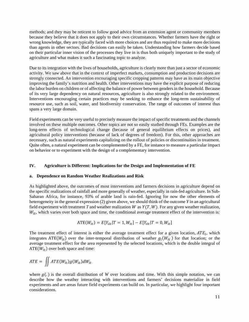
a. Dependence on Random Weather Realizations and Risk As highlighted above, the outcomes of most interventions and farmers decisions in agriculture depend on the specific realizations of rainfall and more generally of weather, especially in rain-fed agriculture. In Sub-Saharan Africa, for instance, 93% of arable land is rain-fed. Ignoring for now the other elements of heterogeneity in the general expression (2) given above, we should think of the outcome Y in an agricultural field experiment with treatment T and weather realization as , . For any given weather realization,

, which varies over both space and time, the conditional average treatment effect of the intervention is:

ATE | 1, | 0, The treatment effect of interest is either the average treatment effect for a given location, , which integrates ATE over the inter-temporal distribution of weather for that location; or the average treatment effect for the area represented by the selected locations, which is the double integral of ATE over both space and time:

where . is the overall distribution of W over locations and time. With this simple notation, we can describe how the weather interacting with interventions and farmers’ decisions materialize in field experiments and are areas future field experiments can build on. In particular, we highlight four important considerations.

12

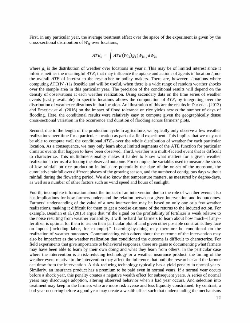
First, in any particular year, the average treatment effect over the space of the experiment is given by the cross-sectional distribution of over locations,

where is the distribution of weather over locations in year t. This may be of limited interest since it informs neither the meaningful that may influence the uptake and actions of agents in location l, nor the overall ATE of interest to the researcher or policy makers. There are, however, situations where computing ATE is feasible and will be useful, when there is a wide range of random weather shocks over the sample area in this particular year. The precision of the conditional results will depend on the density of observations at each weather realization. Using secondary data on the time series of weather events (easily available) in specific locations allows the computation of by integrating over the distribution of weather realizations in that location. An illustration of this are the results in Dar et al. (2013) and Emerick et al. (2016) on the impact of flood tolerance on rice yields across the number of days of flooding. Here, the conditional results were relatively easy to compute given the geographically dense cross-sectional variation in the occurrence and duration of flooding across farmers’ plots. Second, due to the length of the production cycle in agriculture, we typically only observe a few weather realizations over time for a particular location as part of a field experiment. This implies that we may not be able to compute well the conditional over the whole distribution of weather for each particular location. As a consequence, we may only learn about limited segments of the ATE function for particular climatic events that happen to have been observed. Third, weather is a multi-faceted event that is difficult to characterize. This multidimensionality makes it harder to know what matters for a given weather realization in terms of affecting the observed outcome. For example, the variables used to measure the stress of low rainfall on rice production in India are potentially the date of the on-set of the monsoon, the cumulative rainfall over different phases of the growing season, and the number of contiguous days without rainfall during the flowering period. We also know that temperature matters, as measured by degree-days, as well as a number of other factors such as wind speed and hours of sunlight. Fourth, incomplete information about the impact of an intervention due to the role of weather events also has implications for how farmers understand the relation between a given intervention and its outcomes. Farmers’ understanding of the value of a new intervention may be based on only one or a few weather realizations, making it difficult for them to get a precise estimate of the returns to the induced action. For example, Beaman et al. (2013) argue that “if the signal on the profitability of fertilizer is weak relative to the noise resulting from weather variability, it will be hard for farmers to learn about how much--if any--fertilizer is optimal for them to use on their particular plot of land given other possible constraints they face on inputs (including labor, for example).” Learning-by-doing may therefore be conditional on the realization of weather outcomes. Communicating with others about the outcome of the intervention may also be imperfect as the weather realization that conditioned the outcome is difficult to characterize. For field experiments that give importance to behavioral responses, there are gains to documenting what farmers may have been able to learn by their own doing and what they learn from others. In the particular case where the intervention is a risk-reducing technology or a weather insurance product, the timing of the weather event relative to the intervention may affect the inference that both the researcher and the farmer can draw from the intervention. A risk-reducing technology typically has a yield penalty in normal years. Similarly, an insurance product has a premium to be paid even in normal years. If a normal year occurs before a shock year, this penalty creates a negative wealth effect for subsequent years. A series of normal years may discourage adoption, altering observed behavior when a bad year occurs. And selection into treatment may keep in the farmers who are more risk averse and less liquidity constrained. By contrast, a bad year occurring before a good year may create a wealth effect such that understanding the mechanisms

13

underlying the effect of the intervention will be important. In Emerick et al. (2016), the technology tested had no yield penalty. It so happened that a bad year occurred first, identifying the shock-coping value of the innovation. In this case, the first year wealth effect from a seed minikit was sufficiently small not to have meaningful effects on the second year behavioral response. The second year response that occurred under normal weather therefore allowed them to identify the pure risk management response to a reduction in downside risk. As we think of designing future FE in agriculture, the above particularities with regards to weather highlight how such experiments can be designed to make further contributions to our understanding of agriculture: (i) Clustering: Some researchers may want to cluster treatment and control observations to have the

same weather outcomes as much as possible. For example, treatment and control can be located close to the same meteorological station from which the weather realization will be observed by the researcher. This, of course, needs to be done without compromising the risk of spillover effects between treatment and control that we discuss in more detail below.

(ii) Dispersion: To obtain several conditional ATEs will require spreading the experiment over wide geographic areas to observe different weather realizations. The more covariate weather events are, the more geographically dispersed the experiment should be. However, the trade-offs of spreading experiments over large areas include the potential heterogeneity in other factors across a wide area and the difficulty of managing the experiment and collecting data in very distant locations.

(iii) Duration: Having field experiments that run across several time periods to get impacts under different realizations of shocks over time will add great value to our understanding of what works in agriculture, though other factors may interfere with observed outcomes. For example, we may need to allow for learning effects so as not to confound these with outcomes of the particular intervention under study. External conditions will also undoubtedly change, and they may be endogenously affected by the diffusion process itself. The trade-off here is potentially difficulty in maintaining a control group, especially if there is diffusion. .

(iv) Information sharing: If there is rapid loss of learning when there is a sequence of events that makes the innovation unnecessary, then large experiments with information sharing across distant locations will be necessary to preserve the value of learning. This also implies that there will be a lot of fluctuations in individual behavior over time, with many individuals moving in and out of using a particular technology (similar to Suri, 2011), with implications for power calculations in experimental design.

b. The Spatial Dimension of Agriculture: Heterogeneity and Transaction Costs Over the last decade, some of the research in agriculture has highlighted how important local conditions are in economic decision-making in agriculture. Though that is now becoming well recognized, it has also opened up a number of avenues for future research where field experiments can play a role. This heterogeneity of local conditions and their impacts may be quite complex in agriculture for two reasons. First, there are biological or ecological (soil quality for crops) and environmental (climate, altitude) differences across space that make the impacts of farmers decisions (such as which technology to use, whether to use fertilizer, how much fertilizer to use, which crops to grow, which livestock to raise) very heterogeneous (Suri, 2011). Second, there are the more standard dimensions of how the structure of the economy and economic policy affect (broadly) transaction costs. Effective producer prices differ widely according to location and market power and likely from year to year. Factor prices, such as for fertilizer, differ across farmers and may also differ from year to year, especially if these factors are being imported.

14

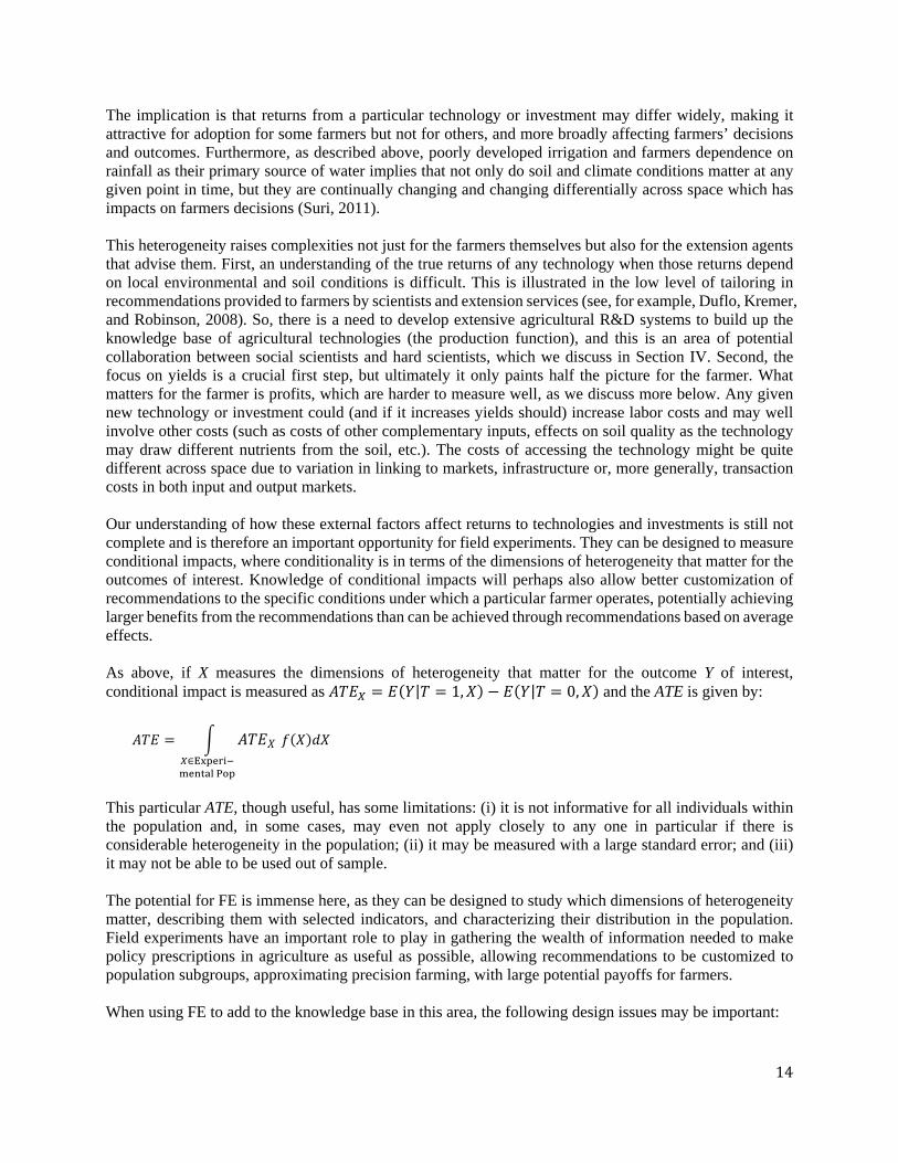
The implication is that returns from a particular technology or investment may differ widely, making it attractive for adoption for some farmers but not for others, and more broadly affecting farmers’ decisions and outcomes. Furthermore, as described above, poorly developed irrigation and farmers dependence on rainfall as their primary source of water implies that not only do soil and climate conditions matter at any given point in time, but they are continually changing and changing differentially across space which has impacts on farmers decisions (Suri, 2011). This heterogeneity raises complexities not just for the farmers themselves but also for the extension agents that advise them. First, an understanding of the true returns of any technology when those returns depend on local environmental and soil conditions is difficult. This is illustrated in the low level of tailoring in recommendations provided to farmers by scientists and extension services (see, for example, Duflo, Kremer, and Robinson, 2008). So, there is a need to develop extensive agricultural R&D systems to build up the knowledge base of agricultural technologies (the production function), and this is an area of potential collaboration between social scientists and hard scientists, which we discuss in Section IV. Second, the focus on yields is a crucial first step, but ultimately it only paints half the picture for the farmer. What matters for the farmer is profits, which are harder to measure well, as we discuss more below. Any given new technology or investment could (and if it increases yields should) increase labor costs and may well involve other costs (such as costs of other complementary inputs, effects on soil quality as the technology may draw different nutrients from the soil, etc.). The costs of accessing the technology might be quite different across space due to variation in linking to markets, infrastructure or, more generally, transaction costs in both input and output markets. Our understanding of how these external factors affect returns to technologies and investments is still not complete and is therefore an important opportunity for field experiments. They can be designed to measure conditional impacts, where conditionality is in terms of the dimensions of heterogeneity that matter for the outcomes of interest. Knowledge of conditional impacts will perhaps also allow better customization of recommendations to the specific conditions under which a particular farmer operates, potentially achieving larger benefits from the recommendations than can be achieved through recommendations based on average effects. As above, if X measures the dimensions of heterogeneity that matter for the outcome Y of interest, conditional impact is measured as | 1, | 0, and the ATE is given by:

∈

This particular ATE, though useful, has some limitations: (i) it is not informative for all individuals within the population and, in some cases, may even not apply closely to any one in particular if there is considerable heterogeneity in the population; (ii) it may be measured with a large standard error; and (iii) it may not be able to be used out of sample. The potential for FE is immense here, as they can be designed to study which dimensions of heterogeneity matter, describing them with selected indicators, and characterizing their distribution in the population. Field experiments have an important role to play in gathering the wealth of information needed to make policy prescriptions in agriculture as useful as possible, allowing recommendations to be customized to population subgroups, approximating precision farming, with large potential payoffs for farmers. When using FE to add to the knowledge base in this area, the following design issues may be important:

15

(i) Heterogeneity of spatial conditions: Ideally, future field experiments would cover a large heterogeneity of spatial conditions so that researchers can better understand whether the benefits of the given farmer decision or investment under study vary by soil type or micro-climate. However, this will come with costs, budgetary as well as the time needed to design, manage, and study an intervention that extends across a large geographical area. An alternative is to work within homogeneous sub-populations, in a way where the homogeneity can be measured based on observable characteristics, leading to findings that can be generalized over these dimensions. Examples of such an approach include Carter et al. (2014) who chose to only work with farmers located along major roads, Burke (2014) who only worked with the highly selected clients of his partner organization, the One Acre Fund and Glennerster and Suri (2015) worked with upland rice farmers.

(ii) Characterizing heterogeneity: There has been little work on (and there is therefore a lot of room for) measuring some of these external factors that matter. An example would be to try to measure soil quality differences to get a sense of local heterogeneity and how much that matters. We know less about how to measure soil quality well, but there are surely many lessons to be learnt from agronomists. There are few studies actively measuring soil quality, with the exception of Fabregas et al. (2015) who study soil testing and the demand for it among farmers in Western Kenya. An alternative is to measure an observable outcome that predicts soil quality deficiencies, as done by Islam (2014), for example, who uses leaf charts in Bangladesh that show how well the plant is taking in nutrients from the soil. In addition, how soil conditions vary over time with climatic events, and with past use of fertilizers, and whether this affects treatment outcomes is an open question. On the climate side, rainfall data is more easily available, both across space and over time. These data can be incorporated to better understand the role of micro-climates in agriculture.

(iii) Heterogeneity along unobservable dimensions. Producers are also heterogeneous along unobserved

dimensions (such as an intrinsic productivity) and in the effort that they are willing to apply to a new process, and hence may enjoy very different benefits from getting access to new technologies. This may explain either large non-compliance or observed low average impact of adoption. In reality, one may be interested in measuring the impact of access to a technology for those who would eventually adopt it rather than for a random sample of the population. Experimental designs can be geared to reveal such heterogeneity and/or foster the desired selection of participants to the experiment. The theory of two-step randomizations to reveal and measure unobserved heterogeneity is developed by Chassang et al. (2012) who suggest the use of “selective trials” as a generalization of RCTs. These selective trials include a mechanism that let the agents reveal their own valuation of the proposed technology, and may furthermore incentivize effort in order to disentangle the role of the product itself from that of the effort applied to its use. Chassang, Dupas, and Snowberg (2013), for example, invited farmers to bid to enhance their chances of winning a new mechanical technology, allowing them to measure the impact of the technology on those most eager to try it. Future field experiments can generalize such approaches, ensuring that the selection mechanism reveals the unobservable characteristics of researcher interest and not other constraints such as wealth or access to liquidity.

(iv) Heterogeneity and learning. Similar heterogeneity may exist along the dimensions that explain the

diffusion of new technologies. If individuals are very different from each other (or their plots are of very different qualities), then there may be limited room for learning. For example, Conley and Udry (2010) find that farmers are more likely to learn from those who are more similar to them or who have a similar experience. Similarly, Tjernstrom (2014) finds that soil quality heterogeneity (at the village level) makes farmers less likely to respond to their peers’ experiences of a new technology. There is still much room to design experiments to better understand the structure of technology diffusion in agriculture, especially with regards to the degree of similarity with specific others in social networks, and how the degree of analogy matters for learning.

16

c. Seasonality and Long Lags

The seasonality of agriculture for cereal or staple crops production makes economic decisions in agriculture more complicated than for, say, a high-turnover vegetable producer. Farmers make investments before or during their planting season, with no returns (i.e., no incomes) until months later when the crop is harvested. Because agricultural cycles depend on rainfall, there is also a commonality in the cycle across all farmers – they all tend to plant and to harvest around the same time. This implies that their demands tend to be quite correlated, especially with regards to labor. Their sales and purchases of food products are also correlated, with a sharp cycle of prices on local markets if there is imperfect tradability. This means that the farmer’s realizations and expectations of output prices are not just indexed by location and year, but also vary within a given year depending on when a farmer chooses to sell. This long cycle in agricultural production also allows for partial revelations of uncertainties and adjustment of behavior along the year. Once rains get started, farmers will update their decisions about the optimal time to plant (Kala, 2014) and what inputs to use. As more of the weather realization is revealed, the farmer will continue to adapt his input choices accordingly. More specifically, these seasonal cycles pose a number of issues for farmers. First farmers face long delays between expenses and revenues. This makes access to credit both all the more important as well as all the more difficult. All the more important because farmers often have to make investments that are costly such as fertilizer purchases long before they earn incomes. All the more difficult to manage as standard microfinance loans with regular payments every week or every month are not relevant since households may have a regular income flow. Second, farmers are often engaged in multiple activities spread over time, so that labor calendars are an important factor in their decisions. For example, if land needs to be cleared for planting, the demand for labor at planting will be high and will involve family labor, possibly supplemented by hired labor. The same is true for harvesting and processing of the crops – both family and hired labor are used. However, in between these two periods, the main activities are crop management, i.e. activities like weeding that are often largely conducted by household labor, partly because less labor is required and partly because monitoring is important for such activities (Bharadwaj, 2010). Designing labor calendars to smooth demands on family labor time becomes an important issue in crop and technological choices (Fafchamps, 1993). This also implies that there will be associated strong seasonalities in other relevant economic variables like the wage rates. Third, due to the long time lags between actions and outcomes, there may be time inconsistencies in decision-making that can have impacts on productivity, sales, and incomes. Commitment devices may be important to overcome these inconsistencies. In this perspective, Duflo et al. (2011) explore a savings commitment device for fertilizer purchases, Brune et al. (2016) a commitment savings product with crop sales paid directly into a bank account as opposed to cash, and Casaburi and Willis (2015) an insurance scheme in Kenya with premiums paid ex-post after harvest. Fourth, the timing of the agricultural cycle leads to an accompanying sales and nutrition cycle in a lot of developing economies. There seems to often be a market failure in crop storage in that most of the farmers who sell grain will tend to sell it at the time of harvests. This implies that sale quantities are high and prices low at harvest. Over the subsequent months, the price of food rises so that right before harvest, there is less food available and its price is quite high. There is evidence that this leads to seasonality in consumption – a lot of farmers report having a hungry season before harvests come in where food availability and consumption are lower than at other times of the year. This seasonality in food consumption could also lead to seasonality in nutrition outcomes of farmers and their household members though this has not been well or widely documented in the literature. Some new agricultural technologies try to shorten the growing cycle of the crop with the hope of allowing multiple cropping over the year with a shorter hungry season, e.g., NERICA rice seed (see Glennerster and Suri, 2015). It remains an open area of research to understanding how farmers should best smooth seasonal fluctuations. One option has been to test ways of improving access to storage (for example, Casaburi et al., 2014 and Burke, 2014). However, storage itself may only be part of the story. Similarly, the hungry season may force farmers into second-best activities such as

17

seasonal migration and participation to the labor market (Fink et al., 2014) that may impact on or take away from the productive activities in agriculture, particularly when technology is labor intensive. On the research side, this seasonality has been important to account for. First, there is a wide heterogeneity in crops and their seasons. Most farmers will invest in a multitude of different crops, with decisions made about one crop affecting others. A technological change in any of these crops (such as adoption of a short duration variety) may affect decision-making in all other crops. Although there may be a season for a lot of cereal and staple crops like maize, wheat, and rice, there are other crops which do not follow such straightforward cycles and may still be a very important part of farmers’ livelihoods. Tree crops like cocoa and coffee are an example, where the tree needs approximately five years to grow before it is productive and so investments are made years before there is a return to them. Another example is cassava which once planted can be left in the ground for multiple years if needs be – farmers often use this as a backup food crop when harvests of their main food crop are poor. Second, it implies long lags between the implementation of any intervention and the outcomes, extending the time horizon for a research project. This usually implies that experiments in agriculture will often span multiple years and are therefore riskier in nature (for example, the second round of the Glennerster and Suri NERICA experiment has been on hold due to the Ebola outbreak in Sierra Leone) with longer term outcomes harder to measure. Given this seasonality and time-lags, future field experiments could build on the following areas: (i) Understanding seasonality. Monitoring outcomes from a given intervention on a seasonal basis rather

than an annual basis could provide important learnings, filling in important steps in the process and reducing dependence on recall data that may be noisy (Beegle et al. 2012). For example, any one intervention may impose short-term seasonal costs, with potential longer-term gains or vice-versa. Measuring all these is important for welfare interpretations. Adoption of a labor-intensive technology, for example, may reduce seasonal migration, with a seasonal cost that is compensated by a higher annual gain. Similarly, data on inputs and behavior should be collected during key periods of the agricultural process. An example is the work of Goldstein and Udry (2008) in Ghana who organized data collection with a round of surveying every six weeks. It is important to note the role that new technologies can play in facilitating this sort of higher frequency data collection: the wide adoption of cell phones in developing economies makes it possible to collect data on labor use, financial transactions, and product sales and purchases by frequent calls (for example, the data collection in the ongoing work of de Janvry et al., 2015 in Jharkhand). There may also be interesting uses of sensors that give real time data, for example, on moisture conditions and on labor movements. We discuss this in more detail in the section below on measurement.

(ii) Successive adjustments. Field experiments that focus on interventions early in the season could be designed to allow adjustments or complementarities later in the season. This would greatly enhance our understanding of complementarities and substitutions across seasons, an area where little is known to date.

(iii) Cost of delays. Studies in agriculture have built in the time lags inherent in agriculture. Missing the

planting season by just a few weeks for any reason can have the heavy cost of a full year lost in the research process. As the timing of planting varies from year to year, for any intervention that needs to happen before planting (like introduction of a new seed or fertilizer), researchers have had to build in enough time to allow for a potentially early planting season that given year. The flip is true for situations when planting happens later than expected in a given year. Finally, a single year may not be enough time to see effects, as discussed above.

d. Market Failures and Non-Separability

18

In the developing country context, production and consumption decisions are integrated. Households cultivate small areas of land and usually provide most of the labor needed on their farms. These households maximize utility, subject to production, and so may not have a single objective defined on their production outlays, such as expected profit or a function of the distribution of net profit to take into account risk and seasonal patterns of income. A household is said to be non-separable when the household’s decisions regarding production (adoption of a technology, use of inputs, choice of activities, desired production levels) are affected by its consumer characteristics (consumption preferences including over leisure, demographic composition, etc.).2 Many papers have demonstrated that a separability test typically fails for smallholder farmers across the developing world (for example, Benjamin, 1992, and Jacoby, 1993). The conceptual framework above (see equation (2)) highlighted how any treatment T introduced to a farmer can affect not just input decisions and hence, outputs, but that the response will also depend on household preferences if separability fails. Some potential symptoms of non-separability are households producing much of what they eat, using exclusively family labor for certain tasks, having excess family labor that cannot find outside employment, etc. These correspond to situations where the household is constrained in the amount of labor or food that it can exchange on the market, or where transaction costs on markets are sufficiently high that the internal equilibrium shadow price of the commodity/factor produced and used by the household makes it suboptimal to either purchase or sell it (Renkow et al., 2004). For example, Fafchamps (1993) shows that farmers select an overall annual cropping pattern that maximally smoothens family labor needs throughout the year. Similarly, farmers maintain the cultivation of several varieties of rice with different maturation lengths or planted at different times to spread the harvest time (Glennerster and Suri, 2015). Farmers often choose to maintain the production of their main staple food (including in India where they have access to cheap government subsidized rice), limiting availability of resources for potentially more profitable cash crops. Since the behavioral models of separable and non-separable households are quite different, we can expect heterogeneity in the uptake of and response to certain agricultural interventions along this dimension. Whether this is important or not of course depends on the intervention. For example, the take up of a new technology may be low because farmers cannot sell any excess output they produce or acquire the labor they need for a labor intensive technology (see Beaman et al., 2013). Alternatively, a farmer may not be able to respond optimally to changes in the price of crops because they are constrained to produce what they want to consume and to use labor as available in the family, which might prevent the household from reallocating its land toward more profitable crops (de Janvry, Fafchamps, and Sadoulet, 1991). There are two relevant aspects of non-separability. First, it is not directly or easily observable, as opposed to say distance to a city or soil quality or rainfall. Whether a household is separable or not is the result of an equilibrium that depends on its resources and preferences. One can sometimes use proxies for this. For example, if the main constraint is on the labor market side (either on sale or purchase), the ratio of available family labor to farm size may provide some indication of the likelihood that the household may be separable or not (Beaman et al., 2013, show that high return to agriculture in Mali is associated with large household size). Future work in this area would account for the quality of the labor force and alternative occupations that determine the opportunity cost of working on the farm and the fact that being “non-separable” is partially an endogenous choice of the household. Second, separable and non-separable households may differ not only in terms of the intensity of their technology uptake or price response, but potentially also across the channels that explain the impact of any intervention. Key with separability are transaction costs in markets that make the household into a net seller 2 We leave aside the cases where risk attitude and time discount are the only ‘preference’ elements that enter the production function,

since these can easily be included in a production model.

19

or a net buyer of a particular food item or of labor. Key with non-separability are resource endowments and internal demand that affect the shadow price of this resource or product. As long as the intervention affects the shadow price without making it affect the effective farm-gate market price as seller or buyer, the household will remain in the non-separability status (Sadoulet and de Janvry, 1995). Future field experiments in agriculture can be designed to shed more light on the issues around separability in the following ways: (i) Household vs. farm as the unit of analysis. Studying the household as a whole as the unit of analysis

will add great value. While any intervention in agriculture may be targeted at the production process of a given crop, hence just the farm operations of a household and perhaps even a given plot, studying the effect on other household decisions can add to what we know about household separability and hence be important in assessing overall outcomes or welfare and shedding light on potential future dynamics around market access.

(ii) Data on production and consumption. There is yet a lot to learn about how interventions will affect both the production and consumption decisions of households. To this end, surveys around a field experiment could collect detailed information not only about farmers’ production but also about their consumption decisions. This can help establish how an intervention targeted at production might be affected by the farmer’s consumption preferences. Similarly, an intervention targeted at consumption, such as a guaranteed employment scheme or a food subsidies program, will have potentially important effects on production decisions.

(iii) Characterizing household-specific market failures. One other open gap in this area is characterization

of prevailing market failures which may well vary from household to household. Particular interventions, for example, that reduce transaction costs and link households to value chains, may transform households from the non-separable to the separable status, with potentially large implications for technology adoption, the elasticity of supply response and ultimately farmer incomes.

(iv) Using FE to test for separation. Testing for separability relies on detecting a causal effect of household

consumption characteristics on production behavior, and has until now been conducted using instrumental variable techniques. An innovative use of field experiments could be to reveal the non-separability of household behavior by, for example, looking at response to an intervention that affects consumption patterns, such as the effective price of food or the opportunity cost of family labor. These would only affect production decisions if the household were non-separable.

e. Spillovers, Externalities, and General Equilibrium Effects In rural settings, people are closely linked to each other, implying that interventions on some individuals may generate a wide range of spillover effects, externalities, and possibly general equilibrium effects. While externalities are not a specificity of agriculture (and hence will be found in many other chapters), spillover effects in the diffusion of new technologies, externalities on the environment, and general equilibrium effects are particularly important in agriculture. In the context of agriculture, we can classify these community links as personal ties among farmers or their households, cost transfers among neighbors through the environment, or price changes through general equilibrium effects in local markets. We discuss each of these in turn briefly. Firstly, a treated farmer will likely inform others in his social network that he is cultivating something new, changing his farming techniques, or adopting a new insurance scheme. This will impact others’ behavior in the community through learning, imitation effects, and potentially economies of scale. Second, there may be large local environmental externalities in agriculture. For example, the effectiveness of biological control

20

methods depends on whether the fields around yours are similarly managed; the cost of underground water depends on the intensity of pumping of farmers extracting water from the same underground basin as you. Finally, as farmers go to sell their products on the local markets, hire labor, and earn some additional income in off-farm activities, prices and wages may change more broadly. Looking back at equation (2) above, for example, externalities and GE effects can affect all aspects of farmers’ decisions via their impacts on the cost side, via input prices (such as wages) and expected output prices. Though these externalities and GE effects may contradict the stable unit treatment value assumption, they should be seen as interesting in themselves, and can, in fact, be a key part of the experimental design. We separate this discussion into three separate areas. First, we look at spillover effects from social interactions, in particular, farmer learning and the diffusion of agricultural technologies. In rural settings, individuals are keenly aware of what their neighbors are doing because they can physically observe their actions. In addition, agricultural communities are closely knit social groups. Individuals within these communities share strong social bonds, which can take the form of informal mutual insurance arrangements, joint production, product sharing, or altruistic behavior. As a result of these two factors, there will undoubtedly be direct spillover effects from one treated farmer to other farmers in the community. The learning (and diffusion) externality around new agricultural technologies has been extensively studied, highlighting when and how learning effects may be important (see the literature section above), For example, we know that the point of entry matters for diffusion (Emerick, 2014, Ben Yishay and Mobarak, 2015 and Beaman et al., 2014). Similarly, the complexity/riskiness of the new technology matters. Some practices or technologies may be easier to learn than others. For example, Tjernström (2014) shows that the extent to which social networks can be relied upon to transmit information depends on the quality of the information environment in which individuals operate. Glennerster and Suri (2015) on the other hand find little evidence of diffusion of a new rice seed in Sierra Leone. Although the literature in this area is vast as highlighted above, there is still room to learn about how extent of diffusion and learning spillovers will depend on the specific structure of the community and its surroundings. Ultimately, there is not overwhelming evidence showing diffusion which leaves large gaps in our understanding of how farmers may learn and an area where field experiments could continue to make important contributions. Second are environmental externalities. There are an additional set of externalities that arise in agriculture that come from crop diseases, pests, water and soil conservation investments, etc. Decisions farmers make about any investments that change the use of water and that affect crop diseases and pests can have broader impacts than just on their own farms. Though there are many examples of such practices (such as integrated pest management, water extraction, etc.), there have been few field experiments to study these spillovers. Water is a very specific resource in agriculture, partly because of its importance to enhance agricultural productivity and partly because it is a communal resource. There are therefore large externalities imposed by water extraction, both across space as well as on future generations (see Foster and Sekhri, 2007, for an example). In addition, the short run benefits and the long run benefits of improved water access are unclear because it is a communal resource across generations (see Hornbeck and Keskin, 2015). There are clearly large gaps in the literature here where field experiments can be designed to help better understand the magnitude of these externalities and their implications for agricultural investments. Third, we discuss the role of market level and GE effects. Agricultural markets are generally small and can be relatively isolated from larger trading networks due to high transaction costs. Local farmers produce a few main crops, and sell any surplus they have in nearby markets. Labor markets are typically local, and land markets even more so. In addition, given the externalities described above, field experiments may be designed as cluster RCTs, i.e., where the level of randomization is a village or a community rather than an individual. This implies, that general equilibrium effects inside the village may well be pervasive and may also occur via non-agricultural outcomes. If the farmers treated by any given intervention see a rise in their agricultural income, they will spend more money on other services provided by the community. This will increase revenue flowing to other non-agricultural activities and contribute to market level changes in prices.

21

Evidence for GE effects is given by Jayachandran (2006) who shows that productivity shocks (in particular, rainfall shocks) cause large changes in the district level wage in India. Similarly, Mobaraq and Rosenzweig (2014) document the general equilibrium effects of rainfall insurance on agricultural wages. The flip side of these isolated markets is that they reveal that transaction costs between markets are high, that there is immense potential for arbitrage, but that there are market failures (potentially credit markets for traders or traders being imperfectly competitive) that restrict these arbitrages from happening. Any given intervention that affects the trading or market environment may well have impacts on prices and hence have broader general equilibrium effects. Understanding these effects is important when wanting to understand the impacts these interventions would have at scale. To date, just a few studies have tried to measure these effects, with much room in the literature for more. Examples include Burke (2014) who tries to measure the price impacts of a crop storage intervention; on-going experiments by de Janvry et al. (2015) on the labor market effects of drought resistant rice seeds in Jharkhand, and the effect of similar technologies on the water market in Bangladesh. In a non-field experiment setting, Evenson and Gollin (2003) showed that prices decreased a lot due to the Green Revolution and this benefited consumers. In general, farmers only benefited from this if there were significant reductions in production costs that were greater than the fall in prices. Finally, there may be strong feedback loops that result in GE effects. The short-term effects of many interventions will differ from their long run impacts. A priori it may be difficult for research to predict what will happen over longer time horizons. As the agricultural and economic systems adapt to a new intervention, many of the original gains from the intervention may be increased or even mitigated. It is important for policy makers to be aware of these effects before they invest in an intervention strategy that they hope will have long run benefits. This scenario is conceptualized in the famous theory of the “technological treadmill” (Cochrane, 1993): early adopters might see larger profits, as they are the first to have access to the new technology. As more and more farmers gain access to the new technology, and “get on the treadmill”, the initial adopters will see their profits decrease. For example, Burke (2014) finds positive effects of a storage intervention in areas where there was a low density of treatment. However, in areas with higher treatment density these positive effects were significantly reduced due to general equilibrium price changes. As prices decline on local markets, the short-run early adopters’ gains typically measured in RCTs will tend to be rapidly dissipated and transferred to consumers on insulated local markets via lower prices, with an ultimately very different incidence of benefits from technological innovations. All these issues have implications for the design of future field experiments. Considering first the case of externalities or spillovers: (i) Designing the FE to avoid or measure spillover effects. Field experiments should be designed to capture

the spillovers that arise (from either learning externalities or the more natural crop disease/pest/water externalities described above) or work to design controls that are largely unaffected by these externalities. On the former, careful designs can also be implemented to accurately measure spillovers (e.g. Baird et al., 2012). The latter would likely affect the level of randomization, which will have cost and power implications.

(ii) Informing spillovers. The field experiment could collect information to measure the effects on surrounding members within the community (even if the unit of analysis is at the village level). This involves measuring effects on farmers that are not treated by the intervention. For example, Glennerster and Suri (2015) designed a field experiment to measure spillovers in the technology, partly because of learning but also because farmers could just share the harvest of the improved rice with their neighbors.

Considering the case of general equilibrium effects and feedback loops:

22

(i) Powering FE to measure GE effects. Measuring general equilibrium effects is challenging. A lot of interventions are small and so the effects they are likely to have on market level prices or other GE outcomes is small, which poses power problems. Future work could focus on larger interventions or designs that vary the concentration of treatment across (say) villages to measure these effects. In addition, some of the effects on non-agriculture could be measure directly through collecting broader data.

(ii) Using market surveys to inform GE effects. Some of these effects will operate through markets. Field

experiments could incorporate the design of market level surveys. These surveys can record prices in nearby markets, as well as wage levels. Researchers could try to measure welfare effects on consumers via falling prices in local markets. As prices fall in local markets, some net seller farmers who did not adopt the technological innovation may start entering the category of more subsistence farmers.

(iii) Measuring the cost side of GE effects. The full set of cost reductions that happen due to any agricultural technology changes may be hard to measure. Researchers conducting field experiments in this area could collect detailed data on as broad a possible set of cost reductions due to a technological intervention as possible.

(iv) Using demand-side interventions to preserve early adopter gains. With shallow local markets, the short

and long-term benefits for adopters of any yield increasing or cost reducing innovation can be dramatically different. This stresses the importance of linking more effectively local to global markets for the benefits from technological change to be at least partially retained by farmers. An open area for new field experiments is therefore to study how supply-side interventions could be complemented with demand-side interventions that may effectively deepen local markets.

(v) Sustaining and scaling-up FE to measure GE effects. Field experiments could extend over longer

periods of time and be scaled up over larger numbers of adopters to trace out how the profitability of the intervention changes as more and more farmers adopt. They can therefore measure whether the benefits to new technologies wear out, and how often new technologies need to be brought in.

f. Measurement

A field experiment will typically aim at measuring how an intervention affects an agricultural outcome along a number of dimensions. As mentioned above, inputs and outputs in agriculture interact in complex ways. For example, promoting the production of a particular cash crop may affect the production of all other crops; promoting fertilizer use on a specific crop may affect the use of other inputs on this crop and also potentially the whole production process. It is therefore important to measure the full set of multiple inputs and outputs, in itself a daunting task due to the extent of the information that needs to be collected and the difficulty of properly characterizing some of these inputs and outputs. In addition, observing the margins on which the farmer has adjusted to the intervention is important in itself, as it can highlight the channels through which the intervention led to the aggregate reduced form effect. For example, Emerick et al. (2016) show how the shock-coping gains from a new risk-reducing rice variety generate further benefits through behavioral responses in risk management. Beaman et al. (2013) show a reduction of the marginal effect of one input through adjustment on another margin. One challenge is to aggregate these outcomes into a performance indicator. In the tradition of agricultural economics, this is done by considering restricted profit that measures the return to the fixed factors or the value of all outputs less the cost of all variable inputs, i.e., using the notation from above, , which involves: (i) establishing the distinction between fixed and variable factors, (ii) measuring all variable inputs, and (iii) measuring all prices that are needed for the aggregation. Finally, while a properly designed field experiment will balance fixed factors over the different treatment arms to allow measuring an average

23

treatment effect over the distribution of these factors, there may be some first-order heterogeneity in the impact of the intervention that ought to be considered so it may be important to measure these fixed factors. In the future, measurement will be key and, from the existing literature, we suggest some areas that can improve the design of future experiments and enhance future learnings:

(i) Concepts difficult to inform. In many cases, farmers may not know the quantities of inputs used or the

quantities of outputs produced. This is particularly the case for an output that is at least partially consumed and that is harvested over a period of time. A good example is cassava that stays in the ground throughout the year (and potentially even multiple years) and is only harvested when needed for consumption, or milk that is collected daily or even twice a day. In this case, surveys cannot ask about total production over the last twelve months as farmers do not think of their production of cassava or milk in this way (Carletto et al. 2015, Zezza et al., 2014). In other cases, the process may be so complex that farmers are not even aware of whether what they do is important (for example, Hanna, et al., 2014). This implies that researchers may have to directly observe input use and/or production rather than ask farmers for it. For the case of continuous use, the researcher may need to rely on recalls or else opt for more frequent data collection (see Goldstein and Udry, 1999). The pervasiveness of cell phones in the developing world will make it much easier to conduct high frequency phone surveys (see de Janvry et al., 2015), though this is not without its own problems as frequent interviews may results in survey fatigue and attrition.

(ii) Quantifying self-provided inputs. Many inputs are self-provided by the household, for example,

household labor. If the household was completely dedicated to agriculture, household labor could be considered as a fixed factor, but this is generally not the case. An additional complication for labor is in defining the proper unit in which to measure labor use, because the work is irregular and dispersed. A labor-day is not a concept used by farmers themselves and hence they do not necessarily know how to quantify it. Similarly, detailed accounting of time use has proved very difficult to do (see Jack et al, 2015 on how they collected time use and their pilots for various ways of collecting time use). Perhaps new electronic tracking devices will provide opportunities to improve data collection on time use.

(iii) Measuring prices. Prices may be observable but often have strong seasonal variations. In a world of

well-functioning markets, neither the spatial nor the seasonal variation of prices presents a conceptual measurement problem. Spatial variation would reflect heterogeneity in transaction costs, and seasonal variation the cost of storage. When there are market failures, with strong seasonal variations, the price chosen to value output can make a difference on the presumed profitability of a farmer. Duflo et al. (2008) chose to price maize at the level it reaches just before the next season’s harvest, as most farmers are then net maize buyers and purchase maize at the end of the season after their own stocks have run out. Beaman et al. (2013) chose to value output at producer prices at the time of harvest. They argue that this, “avoids confounding a potential increase in profits from increased output, with the returns to storage”. Burke (2014) tracks the full time path of maize prices between two harvests since he is interested in the potential returns from arbitraging through storage, with farmers going from sellers when prices are low to buyers when prices are high. Alternatively, Falcao et al. (2014) use traders to obtain high frequency prices from local markets. This is not only an issue for output prices but also for input prices. In general, there is a deficit of information on product and factor prices. If the researcher collects these as self-reports from the farmers, they need to be careful about what set of prices they ask farmers about and whether these are the relevant prices for the problem at hand.

(iv) Pricing family labor. When family labor is sold on the casual labor market, then the opportunity cost of work on the household’s own farm is the wage on that casual market at that particular time (i.e. work on the farm effectively competes with labor allocation outside the farm) (Jack, 2013). However, even in this best-case scenario where there is participation by family labor in the casual labor market,

24

particular on-farm activities may not compete with the off farm time allocation. In this case, the true cost of family labor is the shadow price on their time. If family labor does not work at all off the household farm, then it can be considered a fixed factor shared by all household activities. The shadow price in each activity (and in agriculture) is the equilibrium price internal to the household and is hence endogenous and is not directly observable. It is well known that a large number of family farms do not seem economically viable when family labor is valued at the observed market wage rate in the casual labor market, implying this is not the correct way to value family labor. However, valuing it at the correct shadow price is extremely difficult. In field experiments, we are often more interested in the direction of change in profitability due to a particular intervention than in the absolute value of profits. One solution would therefore be to use a range of labor prices from market price to a fraction of that price and measure the corresponding range of changes in restricted profits as a sufficient indicator of impact. That said, there is room for research that is directed at better understanding agricultural labor markets and the role and productivity of family vs. casual labor in these settings.

(v) Valuing livestock. Many outputs may be difficult to define and/or measure, especially livestock. Livestock plays an important function as a store of value, a producer of organic fertilizers for crops, as well as being a source of income (milk and meat). For many small farmers, their livestock forms a major component of their asset base. Yet, because of the variety of species and ages, the variation in animal quality and herd dynamic, it may be difficult to measure the asset value of the livestock herd. In addition, how their value evolves over time is complex as it depends on investments made by the household as well as age effects on productivity. There has been a lot less research on livestock, which implies that a lot of the measurement issues for livestock have yet to be experimented with and may be more complex than for crops.

(vi) Measuring soil and seed quality. Returns to agricultural technologies and inputs are highly dependent on soil quality, which is often completely unobserved to the researcher. The returns varying with soil quality will, in turn, affect the demand for the new technology. As the use of field experiments in agriculture grows, measuring both true soil quality as well as farmers’ perceptions of it may help advance our understanding of returns. Surveys can elicit farmers’ perceptions, but these may give an incomplete picture of the underlying soil properties. More recently, studies have taken soil samples to help characterize soil quality and potentially discover additional properties of the land not known to the farmer (see Fabregas et al., 2015 and Mahajan et al., 2014). There is still a lot to learn about the relevant variation in soil fertility across plots and over time and how this relates to past use of fertilizers and recent weather events. The same applies to the genetic content of the seeds in use. DNA testing can be used to reveal the origins of seeds, but these tests are expensive, and the extent of relevant heterogeneity in genetic content is not known. These two aspects of soil and seed quality could also make a large difference in the customization of plot-level recommendations.

(vii) Observing technological change. Many field experiments in agriculture study the adoption, diffusion, and impact of technological change. There is much interest in this question for public investment and donor accountability in investing in agricultural research. However, observing technological change can be complex. New seeds may come under the form of a rapid succession of new releases, with each new vintage only making a marginal improvement over the previous. As a sequence, there may be large gains over time, but each release only makes a marginal contribution. This makes it unclear what the appropriate counterfactual is. Only every so often do we observe truly transformative technologies, such as IR6 rice and semi-dwarf wheat cultivars that underpinned the Green Revolution. When “nature does make jumps”, measuring the return to investment in research would use the original traditional varieties as a counterfactual, varieties that may disappear quickly. Future field experiments could be geared to better understanding the dynamics of successive adoption.

25

(viii) Are double blind trials useful in agriculture? A recent measurement issue has been raised is whether the equivalent of double blind trials is useful for FE in agriculture. Researchers have begun to think about behavioral responses to an intervention or a technology in agriculture as separate from the true yield or genetic returns to the technology (see Bulte et al., 2014 for an example). This distinction between genetics and behavior is however, at best, murky. A lot of technologies are only beneficial when they are accompanied by certain practices. These practices typically involve a change in farmer behavior and they are part of the technological package. In addition, any technology that increases yields for a farmer will automatically change some aspects of farmer behavior, for example, labor since there will be more crop to be harvested and therefore more labor required. This is a change in behavior that should be bundled with the technology. The distinction between a behavioral response on the part of the farmer and the technology impact is clearer in the case of Emerick et al. (2016) where they find that the technology helps reduce the yield losses due to flooding (including some element of farmer behavior as recommended by the extension agent). In addition, farmers respond the following year to this change in the risk profile of their outcomes which implies that the second year behavioral response is a lower bound to the role of behavior in contributing to the yield gain of the new technology. In general, there is likely little scope for blind tests in agricultural FE.

(ix) The plot as a unit of analysis. Finally, keeping track of plot-level panels is a challenge as plots are not a static concept. The characterization of production with homogenous conditions is typically at the plot level. Flooding for instance is very much a plot-level event. If the farm is fragmented, as typical in smallholder farming where land has been inherited and divided across family members over generations, a particular household will own several plots with very different features, the very reason why there has been fragmentation (Foster, 2014). Working with plot-level panels would therefore be ideal. However, the definition of a plot is a fluid concept that changes over time. Farmers may not necessarily know how much fertilizer and other inputs they have applied to each plot, while they know how much they have purchased overall. Production from various plots may be combined for threshing, making identification of output per plot difficult. A farmer may change the crop mix on a plot over time, invalidating the previous year’s definition of a given plot and making it impossible to match plots over time, even if one had good GPS maps of plots (which is costly and time consuming).

V. Discussion: Using FE to reveal the production function in agriculture As illustrated above, agriculture is in many aspects different from other productive sectors. Unlike the case of manufacturing, where the production function is a construct of the enterprise, we do not know enough about the true structure of the production function in agriculture. And, because of its link to nature, the production function for agriculture may have more in common with the production function for health than with a standard manufacturing process. One can marvel at the fact that a teaspoon of productive soil typically contains more than one million species of living organisms that are interacting in producing soil fertility. It is now always clear what the full list of inputs into the production function for agricultural products may be – land, labor, climate, soil quality are a small subset of the elements that could possibly matter and each of these cannot easily be represented by a single scalar measure. As an example, the timing of input use is very important for the ultimate outcome. This implies that the combination of quantity and timing of inputs already gives us a long list of entries. We also need to know more about how these inputs may interact with each other in the production function for output: there are almost surely complementarities between labor and soil quality, there are almost surely complementarities between labor and climate. What exact form these complementarities take is not well understood. In the past, the production function has been specified as the product of two sub-functions: a classical production function with the contribution made by factors of production, and a damage function, where damage is done by factors such as pests and bad weather (Lichtenberg and Zilberman, 1986), though this is likely incomplete.

26

In addition, we know little about what farmers themselves know about this production function or how they approximate what this function may be when making their decisions. They may have a very limited or error laden estimate of what the production function looks like, which implies that they are continuously learning themselves and making decisions based on incomplete information. And yet, as T.W. Schultz (1964) taught us, knowing the production function is essential to assess the marginal product of factors and make optimum decisions in factor use. There are three levels at which field experiment research can help reveal the production function. The first is Agricultural Experiment Station (AES) research. Agronomic research has been a pioneer in using statistical experimentation, typically randomization in a Latin Square design analyzed in an ANOVA framework. It was famously introduced into agronomic research by R.A. Fischer at the Rothamsted Experimental Station in Great Britain. Greco-Latin Square designs can be used to test two-by-two combinations of experimental treatments, such as seeds and fertilizer doses. A high yielding variety seed and a traditional seed can thus be tested against various levels of fertilizer use. The problems with AES experiments are twofold. First, the conditions under which the experiment is conducted are generally not reported. For example, what were the levels of irrigation water and pesticides applied in the seed-fertilizer experiment? This limits the applicability of the results obtained. In this case, the particular segment of the production function that has been revealed is not clearly specified. Second, expectedly, with yield as the reported agronomic outcome, the conditions under which the experiment is conducted (such as water, pesticides, and labor practices) are for maximum yield. This does not correspond to what farmers will subsequently do in their farms, where their objective functions will be profit maximization or utility maximization if there is risk aversion. Comparing AES experimental yields with yields in farmers’ fields not surprisingly tend to find that the former are larger than the latter. The second level of useful analysis is in demonstration plots set up by extension agents in farmers’ fields. The farmer is coached by the agent in applying a number of production practices to a new technology. The rest of the production decisions is left to the farmer (in additional to climatic events). The advantage of this approach is that it brings the technology close to potential adopters, with their own objective functions and production conditions. The disadvantage is that the demonstration plot may not always be accompanied by a counterfactual technology (Hancock, 1992). Farmers may be left to compare the treatment outcome to what they does on their own farms, which is for each farmer the next best technology that typically differs from farmer to farmer. There may also not be learning in demonstrating the response function of the new technology. There is room to use the demonstration plot approach to identify the production function by bringing this approach closer to that at AESs. Farmer selection could be formalized and every demonstration plot farmer could be requested to define a counterfactual technology, and cultivate it in an adjacent plot. Information on the impact measured by the difference could then be diffused across farmers so there is an opportunity to learn about the response function. The third is FE in farmers’ fields through randomized control trials. This is the typical seed minikits approach that Dar et al. (2013) followed in testing the flood tolerance value of SwarnaSub1 rice. Minikits are distributed randomly in treatment villages, farmers plant these seeds in a plot of land of their choice (though ideally this should be a randomly chosen plot), they apply their own self-selected cultivation practices in accordance with their objective function, particular climatic events occur, and a yield or any other outcome is observed. If there is a cross-sectional range of climatic events (such as days of flood duration), we can observe the yield advantage of Sub1 over the farmer’s counterfactual seed over that range of events. The advantage is that the outcome corresponds to what farmers will be doing with the technology for their own purpose. The disadvantage is that we only learn about an average treatment effect and some heterogeneity, not the full production function. Because it is difficult to characterize the conditions and events under which the measurement was made, it may be difficult for the farmer to learn from the observed outcomes and it is difficult to use the information to help others learn from these farmers’ outcomes.

27

We see two innovative roles that FE can play in research on agriculture. First, experiments can be designed to reveal the production function. We can gradually uncover the input responses, ideally over a wide range of differing environmental and climatic conditions and begin to better understand what agricultural production functions may look like. This will of course require an almost heroic effort and may lack some of the glamour that motivates economists. A second role that RCTs can play which may be equally important in the short run is to better explore and understand what the implicit production function is that farmers are using in making their own decisions. Here, agronomy meets the social sciences. Understanding this would give us a window into better understanding farmer epistemology, learning and behavior, farmer constraints, and how best can policy respond to inform agents, alter behavior, and relax constraints.

Field experiments can be a powerful tool for project design and policy recommendations in agriculture. The specificities of the production process in agriculture and the agency and social relations in which it is embedded imply an emphasis on design and measurement in these field experiments, matching survey data to data on climactic and soil conditions, so that we can ultimately address questions of first order importance. Above we highlighted opportunities for areas where future field experiments may be able to contribute a great deal to the existing stock of knowledge in this area. Over time, there have been and, no doubt, there will continue to be immense improvements in design and measurement as we adapt to the learnings of earlier experiments and studies. This will be accompanied by improvements in collecting and matching data, including using innovative tools for measurement. As described, field experiments have already contributed important results that help our understanding of the role that agriculture plays in development. The remaining gaps in how to use field experiments in agriculture to address important outstanding development issues create a promising future research agenda.

28

References Armendáriz, Beatriz, and Jonathan Morduch. 2005. The Economics of Microfinance. Cambridge, MA: MIT

Press Books Ashraf, Nava, Xavier Giné, and Dean Karlan. 2009. “Finding Missing Markets (and a Disturbing Epilogue):

Evidence from an Export Crop Adoption and Marketing Intervention in Kenya.” American Journal of Agricultural Economics 91(4): 973-990.

Bai, Jie. 2015. “Melons as Lemons: Asymmetric Information, Consumer Learning, and Seller Reputation.” Working Paper, Department of Economics, Massachusetts Institute of Technology.

Baird, Sarah, Aislinn Bohren, Craig McIntosh, Berk Özler. 2012. “Designing Experiments to Measure Spillover and Threshold Effects.” Policy Research Working Paper Series 6824, The World Bank.

Banerjee, Abhijit, Dean Karlan and Jonathan Zinman. 2015. “Six Randomized Evaluations of Microcredit: Introduction and Further Steps.” American Economic Journal: Applied Economics 7(1): 1-21.

Beaman, Lori, Ariel Ben Yishay, Paul Fatch, Jeremy Magruder, Mushfiq Mobarak. 2014. “Making Networks Work for Policy: Evidence from Agricultural Technology Adoption in Malawi.” Working Paper, Northwestern University.

Beaman, Lori, Dean Karlan, Bram Thuysbaert, and Christopher Udry. 2013. “Profitability of Fertilizer: Experimental Evidence from Female Rice Farmers in Mali.” American Economic Review 103(3): 381-86.

Beaman, Lori, Dean Karlan, Bram Thuysbaert, and Christopher Udry. 2015. “Selection into Credit Markets: Evidence from Agriculture in Mali.” Working Paper, Yale University.

Beegle, Kathleen, Calogero Carletto, and Kristen Himelein. 2012. “Reliability of Recall in Agricultural Data.” Journal of Development Economics 98(1): 34-41.

Ben Yishay, Ariel and Mushfiq Mobarak. 2015. “Social Learning and Incentives for Experimentation and Communication.” Forthcoming Review of Economic Studies.

Benjamin, Dwayne. 1992. “Household Composition, Labor Markets, and Labor Demand: Testing for Separation in Agricultural Household Models.” Econometrica 60(2): 287-322.

Bharadwaj, Prashant. 2010. “Fertility and Rural Labor Market Inefficiencies – Evidence from India.” Journal of Development Economics 115: 217-232.

Brune, Lasse, Xavier Giné, Jessica Goldberg, and Dean Yang. 2016. “Facilitation Savings for Agriculture: Field Experimental Evidence from Malawi.” Economic Development and Cultural Change, 64(2): 187-220.

Bulte, Erwin, Gonne Beekman, Salvatore Di Falco, Lei Pan, and Joseph Hella (2014). “Behavioral responses and the Impact of New Agricultural Technologies: Evidence from a Double-Blind Field Experiment in Tanzania.” American Journal of Agricultural Economics 96(3): 813-30

Burke, Marshall. 2014. “Selling Low and Buying High: An Arbitrage Puzzle in Kenyan Villages.” Working Paper, University of California at Berkeley.

Cai, Hongbin, Yuyu Chen, Hanming Feng and Li-An Zhou. 2010. “Microinsurance, Trust and Economic Development: Evidence from a Randomized Natural Field Experiment.” NBER Working Paper No. 15396.

Cai, Jing, Alain de Janvry and Elisabeth Sadoulet. 2015. “Social Networks and the Decision to Insure.” American Economic Journal: Applied Economics 7(2): 81-108.

Cai, Jing, Alain de Janvry and Elisabeth Sadoulet. 2016. “Subsidy Policies with Learning from Stochastic Experiences.” Working Paper.

Cai, Jing. 2016. “The Impact of Insurance Provision on Households' Production and Financial Decisions.” American Economic Journal: Economic Policy 8(2): 44-88.

Carletto, Gero, Dean Jolliffe, and Raka Banerjee. 2015. “From Tragedy to Renaissance: Improving Agricultural Data for Better Policies.” The Journal of Development Studies 51(2): 133-148.

Carter, Michael, Rachid Laajaj, and Dean Yang. 2014. “Subsidies and the Persistence of Technology Adoption: Field Experimental Evidence from Mozambique.” NBER Working Paper No. 20465.

29

Casaburi, Lorenzo, Rachel Glenenrster, Tavneet Suri and Sullay Kamara. 2014. “Providing Collateral and Improving Product Market Access for Smallholder Farmers: A Randomised Evaluation of Inventory Credit in Sierra Leone.” 3ie Impact Evaluation Report 14, July 2014.

Casaburi, Lorenzo, Michael Kremer, Sendhil Mullainathan, and Ravindra Ramrattan. 2014. “Harnessing ICT to Increase Agricultural Production: Evidence From Kenya.” Harvard University.

Casaburi, Lorenzo, and Tristan Reed. 2014. “Interlinked Transactions and Pass-Through: Experimental Evidence from Sierra Leone.” Stanford Institute for Economic Policy Research, Stanford University.

Casaburi, Lorenzo, and Jack Willis. 2015. “Time vs. State in Insurance: Experimental Evidence from Contract Farming in Kenya. Working Paper, Stanford University.

Chassang, Sylvain, Gerard Padró i Miquel, and Erik Snowberg. 2012. “Selective Trials: A Principal-Agent Approach to Randomized Controlled Experiments” American Economic Review 102(4): 1279–1309.

Chassang, Sylvain, Pascaline Dupas, and Erik Snowberg. 2013. “Selective Trials for Agricultural Technology Evaluation and Adoption: A Pilot.” ATAI Pilot Project, CEGA, University of California Berkeley.

Cochrane, Willard. 1993. The Development of American Agriculture: A Historical Analysis. Minneapolis, MN: University of Minnesota Press.

Cole, Shawn, Xavier Giné, and James Vickery. 2014. “How Does Risk Management Influence Production Decisions? Evidence from a Field Experiment.” Forthcoming Review of Financial Studies.

Conley, Timothy, and Christopher Udry. 2010. “Learning about a New Technology: Pineapple in Ghana." American Economic Review 100(1): 35-69.

Dar, Manzoor, Alain de Janvry, Kyle Emerick, David Raitzer, and Elisabeth Sadoulet. 2013. “Flood-tolerant rice reduces yield variability and raises expected yield, differentially benefitting socially disadvantaged groups.” Scientific Reports 3, Article number 3315, November 22.

de Janvry, Alain, Marcel Fafchamps, and Elisabeth Sadoulet. 1991. “Peasant Household Behavior with Missing Markets: Some Paradoxes Explained.” Economic Journal 101(409): 1400-17.

de Janvry, Alain, Elisabeth Sadoulet, Kyle Emerick, and Manzoor Dar. 2015. “The Impact of Drought-Tolerant Rice on Local Labor Markets in India”. Work in Progress.

Duflo, Esther, and Rohini Pande. 2007. “Dams.” Quarterly Journal of Economics 122(2): 601-46. Duflo, Esther, Michael Kremer, and Jonathan Robinson. 2008. “How High are Rates of Return to Fertilizer?

Evidence from Field Experiments in Kenya.” American Economic Review, Papers and Proceedings 98(2): 482-88.

Duflo, Esther, Jonathan Robinson, and Michael Kremer. 2011. “Nudging Farmers to Use Fertilizer: Theory and Experimental Evidence from Kenya.” American Economic Review 101(6): 2350–90.

Duflo, Esther, Daniel Keniston and Tavneet Suri. “Technology Adoption in Agriculture: Evidence from a Randomized Experiment in Rwanda”. Work in Progress.

Dupas, Pascaline. 2014. “Getting Essential Health Products to Their End Users: Subsidize, but How Much?” Science 345(6202): 1279-1281.

Elabed, Ghada, and Michael Carter. “Ex-ante Impacts of Agricultural Insurance: Evidence from a Field Experiment in Mali.” Working paper, June 2015.

Emerick, Kyle, Alain de Janvry, Elisabeth Sadoulet, and Manzoor Dar. 2016. “Technological Innovations, Downside Risk, and the Modernization of Agriculture.” American Economic Review 106(6): 1537-61.

Emerick, Kyle. 2014. “The Efficiency of Trading in Social Networks: Experimental Measures from India.” Working Paper, Tufts University.

Evenson, Robert, and Douglas Gollin. 2003. “Assessing the Impact of the Green Revolution, 1960-2000.” Science 300(758): 1078710.

Fabregas, Raissa, Michael Kremer, Martins Odendo, Jonathan Robinson, and Frank Schilbach. 2015. “Evaluating Agricultural Information Creation and Dissemination in Western Kenya.” Work in Progress.

Fafchamps, Marcel. 1993. “Sequential Labor Decisions under Uncertainty: An Estimable Household Model of West-African Farmers.” Econometrica 61 (5): 1173-1197.

30

Fafchamps, Marcel, and Bart Minten. 2012. “Impact of SMS-Based Agricultural Information on Indian Farmers.” World Bank Economic Review 26(3): 383-414.

Falcao, Lauren, Paul Gertler, and Craig McIntosh. 2014. E-Warehousing for Smallholder Farmers. ATAI Project, JPAL.

Fink, Gunther, Kelsey Jack, and Felix Masiye. 2014. “Seasonal Credit Constraints and Agricultural Labor Supply: Evidence from Zambia.” NBER Working Paper 20218.

Foster, Andrew, and Mark Rosenzweig. 1995. “Learning by Doing and Learning from Others: Human Capital and Technical Change in Agriculture.” Journal of Political Economy 103 (6): 1176–1209.

Foster, Andrew, and Sheetal Sekhri, 2007. “Can Expansion of Markets for Groundwater Decelerate the Depletion of Groundwater Resource in Rural India?” Brown University Working Paper.

Foster, Andrew. 2014. “Spillovers, Coordination Failures and Land Fragmentation.” Working Paper, Brown University.

Giné, Xavier, and Dean Yang. 2009. “Insurance, Credit, and Technology Adoption: Field Experimental Evidence from Malawi.” Journal of Development Economics 89(2009) 1-11.

Glennerster, Rachel, and Tavneet Suri. 2015. “Measuring the Effects of NERICA, Short Duration Rice, on Harvest Prices.” ATAI Project, MIT.

Goldstein, Markus, and Christopher Udry. 1999. “Agricultural Innovation and Resource Management in Ghana.” International Food Policy Research Institute, Washington D.C.

Goldstein, Markus, and Christopher Udry. 2008. “The Profits of Power: Land Rights and Agricultural Investment in Ghana.” Journal of Political Economy 116(6): 981-1022.

Hancock, John. 1992. “Extension Education: Conducting Effective Agricultural Demonstrations.” Cooperative Extension Service, College of Agriculture, University of Kentucky.

Hanna, Rema, Sendhil Mullainathan, and Josh Schwartzstein. 2014. “Learning by Noticing: Theory and Evidence through a Field Experiment.” Quarterly Journal of Economics 129(3): 1311-53.

Hornbeck, Richard, and Pinar Keskin. 2015. “Does Agriculture Generate Local Economic Spillovers? Short Run and Long Run Evidence from the Ogallala Aquifer.” American Economic Journal: Economic Policy, 7(2): 192-213

Islam, Mahnaz. 2014. “Practice Does Not Make Perfect: Understanding Fertilizer Mismanagement in Bangladesh through Leaf Color Charts.” Working Paper, Harvard University.

Jack, Kelsey. 2011. “Market Inefficiencies and the Adoption of Agricultural Technologies in Developing Countries.” White paper prepared for the Agricultural Technology Adoption Initiative (ATAI), JPAL (MIT) / CEGA (Berkeley).

Jack, Kelsey. 2013. “Private Information and the Allocation of Land Use Subsidies in Malawi.” American Economic Journal: Applied Economics 5(3): 113-35

Jack, William, Joost de Laat, Michael Kremer and Tavneet Suri. 2015. “Joint Liability, Asset Collateralization, and Credit Access: Evidence from Rainwater Harvesting Tanks in Kenya.” Working Paper.

Jacoby, Hanan. 1993. “Shadow Wages and Peasant Family Labor Supply: An Econometric Application to the Peruvian Sierra.” Review of Economic Studies 60: 903-921.

Jayachandran, Seema. 2006. “Selling Labor Low: Wage Responses to Productivity Shocks in Developing Countries.” Journal of Political Economy 114(3): 538-575.

Kala, Namrata. 2014. “Ambiguity Aversion and Learning in a Changing World: The Potential Effects of Climate Change from Indian Agriculture.” Working Paper, Yale University.

Karlan, Dean, Robert Osei, Isaac Osei-Akoto, and Christopher Udry. 2014. “Agricultural decisions after relaxing credit and risk constraints.” The Quarterly Journal of Economics 129 (2): 597-652.

Lichtenberg, Erik, and David Zilberman. 1986. “The Econometrics of Damage Control: Why Specification Matters.” American Journal of Agricultural Economics 68(2): 261-73.

Mahajan, Aprajit, Enrique Seira, and Xavier Gine. 2014. “A Multiple Interventions Approach to Increasing Technology Adoption with a View Towards Scaling-Up: Evidence from Mexico.” BASIS Proposal.

31

Matsumoto, Tomoya, Takashi Yamano, and Dick Sserunkuuma. 2013. “Technology Adoption and Dissemination in Agriculture: Evidence from Sequential Intervention in Maize Production in Uganda.” GRIPS Discussion Papers 13-14, National Graduate Institute for Policy Studies.

McIntosh, Craig, Alexander Sarris, and Fotis Papadopoulos. 2013. “Productivity, Credit, Risk, and the Demand for Weather Index Insurance in Smallholder Agriculture in Ethiopia." Agricultural Economics (44):399–417.

Mobarak, Mushfiq, and Mark Rosenzweig. 2014. “Risk, Insurance and Wages in General Equilibrium.” Working Paper, Yale University.

Mobarak, Mushfiq, and Mark Rosenzweig. 2013. “Selling Formal Insurance to the Informally Insured.” Working paper, Yale University.

Renkow, Mitch, Daniel Hallstrom, and Daniel Karanja. 2004. “Rural Infrastructure, Transactions Costs and Market Participation in Kenya.” Journal of Development Economics 73(1): 349-367.

Sadoulet, Elisabeth, and Alain de Janvry. 1995. Quantitative Development Policy Analysis. Baltimore: The Johns Hopkins University Press.

Schilbach, Frank. 2015. Essays in Development and Behavioral Economics. Doctoral dissertation, Harvard University, Graduate School of Arts & Sciences.

Schultz, T.W. 1964. Transforming Traditional Agriculture. New Haven: Yale University Press. Suri, Tavneet. 2011. “Selection and Comparative Advantage in Technology Adoption.” Econometrica

79(1): 159–209. Tjernström, Emilia. 2014. “Signals, Similarity and Seeds: Social Learning in the Presence of Imperfect

Information and Heterogeneity.” Working Paper, University of California at Davis. Visaria, Sujata and Mitra, Sandip and Mookherjee, Dilip and Torero, Maximo, 2015. Asymmetric

Information and Middleman Margins: An Experiment with Indian Potato Farmers. HKUST IEMS Working Paper No. 2015-29.

World Bank. 2007. Agriculture for Development-World Development Report. The World Bank. World Bank. World Bank Development Indicators. Online Database. The World Bank. Zezza, Alberto, Giovanni Federighi, Kalilou Adamou, and Pierre Hiernaux. 2014. “Milking the Data:

Measuring Income from Milk Production in Extensive Livestock Systems: Experimental Evidence from Niger.” Research working paper WPS 7114. Washington, DC: World Bank Group.