Field comparison of network Sun photometers · Systems (YES) Multifilter Rotating Shadowband...

Field comparison of network Sun photometers

L. J. Bruce McArthur,1 David H. Halliwell,2 Ormanda J. Niebergall,2 Norm T. O’Neill,3

James R. Slusser,4 and Christoph Wehrli5

Received 19 September 2002; revised 3 February 2003; accepted 25 March 2003; published 2 October 2003.

[1] Measurements of aerosol optical depth have become more numerous since the mid-1990s with the onset of commercially available, high-quality, low-maintenance automaticinstrumentation. The development of several networks for aerosol measurements, andthe next day availability of preliminary data for some, have further enhanced interest in theproducts this type of measurement can provide. With several networks operating globallyand others operating either regionally or continentally within North America thecomparability of the data emanating from the various archive centers is an important issue.The Bratt’s Lake Observatory operates four separate types of Sun photometers inconjunction with three different networks: Aerosols in Canada, Global Atmosphere Watch,and the U.S. Department of Agriculture UV-B Monitoring Program. Data collected duringthe summer of 2001, following the protocols established by the networks and theMeteorological Service of Canada, were analyzed to determine the comparability amongthese networks. As the instruments and conversion algorithms are similar to othernetworks from around the globe, it is believed that the results of this comparison can betransferred, at least in part, to other operational networks. The results of the 3-month studyindicate that the data obtained from the networks that operate direct-pointinginstruments are very comparable, being within ±0.01 of an optical depth for instantaneousmeasurements during cloud-free line-of-sight conditions. Over the length of thecomparison the root mean square difference of aerosol optical depth at 500 nm betweenthe direct sun-pointing instruments was 0.0069. The rotating shadowband instruments didnot perform as well. These results indicate that the data from well-maintained networksof direct sun-pointing photometers can provide data of the quality necessary to comparestations from across the globe. INDEX TERMS: 0305 Atmospheric Composition and Structure:

Aerosols and particles (0345, 4801); 0360 Atmospheric Composition and Structure: Transmission and

scattering of radiation; 0394 Atmospheric Composition and Structure: Instruments and techniques; 1640

Global Change: Remote sensing; 3359 Meteorology and Atmospheric Dynamics: Radiative processes;

KEYWORDS: Sun photometer, AOD, Angstrom coefficient

Citation: McArthur, L. J. B., D. H. Halliwell, O. J. Niebergall, N. T. O’Neill, J. R. Slusser, and C. Wehrli, Field comparison of

network Sun photometers, J. Geophys. Res., 108(D19), 4596, doi:10.1029/2002JD002964, 2003.

1. Introduction

[2] Optical depth measurements are regularly acquiredusing Sun photometers or shadowband radiometers from anumber of networks around the world. These measurementsare used to provide global aerosol climatologies [Holben etal., 2001; Michalsky et al., 2001] and to validate satellite

aerosol observations on the one hand and provide atmo-spheric corrections for satellite retrievals on the other[Fedosejevs et al., 2000]. Probably the best known of thesenetworks is the Aerosol Robotic Network (AERONET)[Holben et al., 1998], a NASA-operated network thatemploys the Cimel Sun photometer. The Canadian compo-nent of this network is Aerosols in Canada (AEROCAN)[Bokoye et al., 2001]. The Global Atmosphere WatchProgramme is presently equipping a number of its back-ground sites with Precision Filter Radiometers (PFRs),designed and manufactured at Physikalisch-Meteorolo-gisches Observatorium/World Radiation Centre (PMOD/WRC) (Davos, Switzerland) as part of the Swiss contribu-tion to the World Meteorological Organization. Also capa-ble of providing aerosol optical depth measurements withinthe continental United States (including two Canadianstations) is the U.S. Department of Agriculture (USDA)UV-B Monitoring Program using Yankee EnvironmentalSystems (YES) Multifilter Rotating Shadowband Radio-

JOURNAL OF GEOPHYSICAL RESEARCH, VOL. 108, NO. D19, 4596, doi:10.1029/2002JD002964, 2003

1National Atmospheric Radiation Centre, Meteorological Service ofCanada, Toronto, Ontario, Canada.

2Bratt’s Lake Observatory, Meteorological Service of Canada, Wilcox,Saskatchewan, Canada.

3Le Centre d’applications et de recherches en teledetection, Universitede Sherbrooke, Sherbrooke, Canada.

4U.S. Department of Agriculture UV-B Monitoring and ResearchProgram, Colorado State University, Fort Collins, Colorado, USA.

5Physikalisch-Meteorologisches Observatorium/World RadiationCentre, Davos, Switzerland.

Copyright 2003 by the American Geophysical Union.0148-0227/03/2002JD002964$09.00

AAC 1 - 1

meter (MFRSR) in both the UV and visible portions of thespectrum. These instruments are operated by the NaturalResource Ecology Laboratory (Colorado State University)[Bigelow et al., 1998]. A second regional network operatingMFRSR instruments in the United States is the QuantitativeLinks program [Michalsky et al., 2001]. Further examples ofregional networks are the Swiss national network [Ingold etal., 2001], which uses a sun-pointing photometer, theAustralian combined networks composed of 16 AustralianBureau of Meteorology stations that operate Carter-ScottSP01A and SP02 sun-pointing photometers, and threestations of the Commonwealth Scientific and IndustrialResearch Organisation Aerosol Ground Station Networkthat use the Cimel CE318 sun/sky photometer [Mitchelland Forgan, 2003].[3] With the ever-increasing use of the World Wide Web

as a means of propagating data quickly, results from anumber of networks are now available within hours of theobservations being made. This rapid publication of dataencourages users from various disciplines to create value-added products by combining observations from variousnetworks. Therefore it is important to know if the variousproducts distributed in near-real-time, whether they beaerosol optical depth (AOD) or a parameter calculated fromAOD, such as Angstrom’s coefficients, are comparable.[4] The most commonly defined forms of AOD are based

on the Beer-Lambert law for monochromatic radiation andare expressed, depending on the complexity of the air massterms used, by

da ¼ ln I0=Ið Þm�1 �Xi

ti ð1Þ

or

da ¼ ln I0=Ið Þ �Xi

timi

" #m�1

a ; ð2Þ

where for a given wavelength (l), the AOD (da) is afunction of the monochromatic spectral flux measured at thesurface (I), the extraterrestrial monochromatic flux (I0)corrected for the sun-earth distance, the optical air mass (m),and the optical depth of the various atmospheric constitu-ents (di) that affect the transmission through the atmospheresuch as molecular scattering and gaseous absorption. Themajor difference between the two methods is in thedescription of the vertical structure of atmospheric con-stituents. Equation (1), which is more commonly used,assumes that all constituents are vertically distributed in thesame manner, while equation (2) recognizes that aerosolsand atmospheric gases can be better modeled usingindividual scale-height air mass values (mi).[5] The formulation in the optical domain of Angstrom’s

[1929] relationship, which is based on the simplest form ofthe aerosol size distribution for particles between �0.08 mmand �2 mm, is the Junge power law (r � g) expression[Junge, 1963], between optical depth and wavelength

dl ¼ b l=l0ð Þ�a; ð3Þ

where dl is the aerosol optical depth at wavelength l (in mm),l0 is defined as the 1-mmwavelength. The parameter a is the

log-log slope of the curve (g - 2) and is sensitive to theaerosol size distribution; as a increases, the number of smallparticles increases. The parameter b is the optical depth at awavelength of 1 mm and is proportional to the verticallyintegrated aerosol concentration.[6] Historically, instrument comparisons have consisted

of bringing a number of instruments together to a singlelocation for a period of several days to several weeks [e.g.,Schmid et al., 1999]. These types of comparisons areessential to moving forward the frontiers of instrumentscience. However, there may be little or no relation betweenthe results of these intensive comparisons and the resultsfrom the same instruments when placed in an operationalnetwork setting. The comparison that is being reported onprovides insight into the quality of data output by instru-ments when cared for following operational protocolsdesigned by the various network investigators. Furthermore,the data that are compared comprise the normal productassociated with the various data centers responsible for theroutine handling of the measurements. Therefore the resultsof this comparison should provide an understanding both ofthe comparability between networks and of the overall dataquality of the networks represented.

2. Comparison Locale

[7] The AERONET, Global Atmosphere Watch (GAW),and USDA networks intersect at the Bratt’s Lake Observa-tory (BLO) (50�170N, 104�420W), a Baseline Surface Radi-ation Network (BSRN) station in the southern Canadianprairies. In addition to these network observations the observ-atory derives optical depths from aMeteorological Service ofCanada (MSC) YES visible MFRSR and a pair of MiddletonSP01A Sun photometers, similar to those used by theAustralian Bureau of Meteorology in the combined Austra-lian networks. The inclusion of the GAW PFR photometer inlate spring 2001 provided the opportunity to compare theoutput of each of these different types of instruments over alonger period of time than the more normal high-intensity,short-duration, multinational comparison.[8] The BLO is located in the southern Canadian prairies

�60 km north of the Canada-U.S. border and 25 km southof Regina, Saskatchewan. Geographically, the area isextremely flat with the primary activity being low-intensityagriculture, primarily wheat. The climate is continental, thenormal mean summertime temperature being �18�C. Con-vective cloud occurs most days throughout the summer, butprecipitation is low. The summer of 2001 was particularlydry, and, consequently, the influence of windblown partic-ulates exceeded normal levels. There are no significantlocal sources of anthropogenic air pollution, so aerosoloptical depths are normally low [Fedosejevs et al., 2000],although they peak during the summer period. Low aerosoloptical depths present particular problems with networkconfigurations where assumptions are made concerningpressure and absorbing gases.[9] While measurements of many radiation, meteorolog-

ical, and air quality variables are made at the observatory,two that significantly impact on the reduction of Sunphotometer voltages to aerosol optical depth are air pressureand ozone amount. The local surface pressure is measuredonce per second with a 1-min average recorded. Because

AAC 1 - 2 MCARTHUR ET AL.: NETWORK SUN PHOTOMETER COMPARISON

pressure can vary significantly throughout the day andRayleigh scatter is significant at short wavelengths whenthe optical depth is small, the coinciding pressure was usedin the calculation of Rayleigh optical depth for the GAWinstrumentation. Columnar ozone is measured up to 40 timesper day using a Brewer Mk IV spectrophometer [Kerr andMcElroy, 1993] based on the ozone absorption coefficientsof Bass and Paur [1985]. For the purposes of this compar-ison the daily mean column ozone was used to calculate thevalue of ozone absorption. Figure 1 shows the variation inmean daily temperature, pressure, ozone, and 500-nmaerosol optical depth, as determined from the Cimel Sunphotometer data, for the comparison period.

3. Instrumentation and Network Protocols

[10] This section will briefly describe the network, theinstrumentation used in the network, the protocols associ-ated with the maintenance of the equipment, and thealgorithms associated with the reduction of the electricalsignal to aerosol optical depth, including any screening thenetwork uses to quality assure the data with respect tointerference from clouds. Table 1 provides a brief overviewof each of the instruments, including pertinent facts associ-ated with the collection and analysis of the data.

3.1. AEROCAN

[11] AEROCAN [Boyoke et al., 2001] is the Canadiansubset of the NASA AERONET federation of Sun photom-eter networks [Holben et al., 1998] and consists of stationsmostly in southern Canada. As part of AERONET, CimelSun photometers are used exclusively, and the networkprotocols set out by AERONET (available at http://aeronet.gsfc.nasa.gov/ (under ‘‘Operations’’)) are followed withrespect to maintenance. The Cimel Electronique 318Aphotometer is a dual collimator instrument for the measure-ment of direct solar and sky radiances. The direct sun modeis measured using a solar collimator with a 1.2� field ofview. Sky mode observations are made using a similarcollimator with the incorporation of lenses to increase thesignal. The instrument contains eight ion-assisted deposition

interference filters housed in a rotating wheel. The directbeam signal is measured with a UV-enhanced siliconphotodiode. Corrections for photodiode and filter tempera-ture dependencies are made based on an internal tempera-ture sensor. The optical assembly is attached to a robot armthat uses a four-quadrant sensor to point the instrument withan accuracy of 0.1�. Further details on the filter configura-tion are in Table 1, and a more complete description is givenby Holben et al. [1998]. The Sun photometer is routinelycalibrated by shipping the instrument to NASA Goddard,where outdoor comparisons are made with a group ofstandard Cimel Sun photometers that are calibrated atMauna Loa, Hawaii. The collected data are transmitteddirectly to AERONET, where automatic quality assuranceis performed, including cloud screening [Smirnov et al.,2000]. Part of this quality assurance procedure determinesthe data collection and data transmission offsets for indi-vidual instruments to within 1 s. Data are classified by leveldepending upon the quality assurance processing per-formed. Level 1.0 data has the preinstallation calibrationcoefficients applied to the data. Data that have been auto-matically cloud screened is classified as level 1.5 and areavailable from the AERONET Web site usually the dayfollowing the measurements. A higher-quality data productthat incorporates a calibration stability check is availablefollowing the recalibration of the Cimel instrument(level 2.0). The Cimel instrument used for this comparisonwas calibrated immediately before the comparison period.Because of a mechanical failure in the instrument, thecomparison was terminated and the instrument returned toNASA Goddard for repair and a postcomparison calibration.All three levels of data were used in this comparison. Levels1.0 and 1.5 were employed in determining cloud-screeningstatistics, while the level 2.0 data were used for the AODcomparison. In this particular comparison, differences inAOD between the level 1.5 and level 2.0 data wereinsignificant.[12] Although the Cimel is capable of measuring many

more parameters than the direct beam spectral extinction,these are not considered in this comparison. Level 1.0extinction data is observed once every 15 min and recordedonly if the signal does not indicate severe cloud-inducedinstability (coarse precloud screening triplet rejection) or ifprecipitation is occurring. Subsequent level 1.5 cloud-screening criteria include a triplet check (temporal stabilityof three optical depth measurements) and a second-ordertemporal derivative constraint [Smirnov et al., 2000]. Asthis is the most infrequent measurement of aerosol opticaldepth, the data from the other instruments involved in thecomparison will be presented initially at this temporalinterval.[13] The remote nature of many of the AERONET

locations has required that both the surface pressure (neededfor the calculation of Rayleigh optical depth) and thecolumnar ozone amount (needed to calculate ozone absorp-tion in the Chappuis band) be estimated. The former isbased upon surface elevation and the standard atmosphere,while the latter uses a 5� gridded ozone climatology basedon the work of London et al. [1976]. The determination ofRayleigh optical depth follows Bucholtz [1995], and theozone absorption coefficients used are from Vigroux[1953]. Eck et al. [1999] give the maximum uncertainties

Figure 1. Variation in meteorological variables during thecomparison. Daily temperature, pressure, ozone amount,and 500-nm aerosol optical depth (Aerosol Robotic Net-work (AERONET) Cimel).

MCARTHUR ET AL.: NETWORK SUN PHOTOMETER COMPARISON AAC 1 - 3

Table

1.DescriptionofNetwork

Photometers/RadiometersThat

Participated

intheNetwork

ComparisonofAerosolOpticalDepth

Instrument

Wavelengths,

nm

Methodof

Calibration

Methodof

Measurement

Sam

pling

Rate

O3

Amount

Atm

ospheric

Pressure

Cloud

Screening

Reference

AEROCAN

Cim

el340,379,437,

498,669,

871,1021;

fullwidth

athalf

maxim

um

(FWHM)

10nm

comparisonwith

standardinstrument

directSun,activetracking;

filter

wheel,single

detector;

fieldofview

(FOV)1.2�

Observationtime,

8s;

samplingfrequency,

variable,dependent

uponday

length

tabular;5�lat.

andlong.

clim

atology

based

onsite

elevation;

586.7

m

Smirnovet

al.

[2000]

Bokoye

etal.[2001]

andHolben

etal.

[1998]

GAW

PFR

367.8,411.9,

500.4,862.9;

FWHM

3.8–5.4

nm

comparisonwithabsolute

spectral

radiometer;

refined

Langleyand

ratio-Langleycalibration


multiple

sensors;FOV

2.5�

once

per

minute

on-siteBrewer

column

ozone

measurement

on-board

pressure

transducer

combinationof

Smirnovet

al.

[2000]and

Harrisonand

Michalsky

[1994]

Wehrli[2000]

Middleton

SP01A

368,412,502a,

502b,675,

778,812,862;

FWHM

5nm

Langleycalibration

(equation(1))


multiple

detectors;FOV

2.4�

once

per

minute

on-siteBrewer

column

ozone

measurement

localmean

daily

pressure

modifiedHarrison

andMichalsky

[1994]

USDA

MFRSR

(Yankee

Environmental

System

s,Inc.)

415,500,610,

665,860,

940;FWHM

10nm

on-siteprogressiveLangley

calibration(equation(1))

residual

calculationfrom

global

anddiffuse

irradiance

measurements;multiple

detectors;equivalentFOV

20saveraged

over

3min

300Dobson

units

based

onsite

elevation;

586.7

m

none

Harrisonet

al.[1994]

andBigelow

etal.

[1998]

MSC

MFRSR

415.8,496.4,

613.6,671.6,

869.5,937.5;

FWHM

10nm

on-siteLangleycalibration

(equation(1))

residual

calculationfrom

global

anddiffuse

irradiance

measurements;multiple

detectors;equivalentFOV

15saveraged

over

1min

on-siteBrewer

column

ozone

measurement

localmean

daily

pressure

none

Harrisonet

al.[1994]


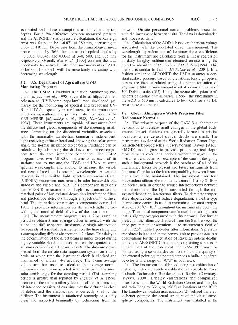
associated with these assumptions as equivalent opticaldepths. For a 3% difference between measured pressureand the AERONET static pressure calculation, the Rayleigherror was found to be �0.021 at 380 nm, decreasing to0.007 at 440 nm. Departures from the climatological meanozone amount by 50% alter the aerosol optical depths by�0.0036, 0.0045, and 0.0063 at 340, 500, and 675 nm,respectively. Overall, Eck et al. [1999] estimate the totaluncertainty for network instrument measurements of AODto be �0.010–0.021, with the uncertainty increasing withdecreasing wavelength.

3.2. U.S. Department of Agriculture UV-BMonitoring Program

[14] The USDA Ultraviolet Radiation Monitoring Pro-gram [Bigelow et al., 1998] (available at http://uvb.nrel.colostate.edu/UVB/home_page.html) was developed pri-marily for the monitoring of spectral and broadband UV-B and UV-A, especially in rural areas, to determine theireffect on agriculture. The primary instrument used is theYES MFRSR [Michalsky et al., 1988; Harrison et al.,1994]. These instruments are capable of measuring boththe diffuse and global components of the incoming irradi-ance. Correcting for the directional variability associatedwith the nominally Lambertian (angularily independent)light-receiving diffuser head and knowing the solar zenithangle, the normal incidence direct beam irradiance can becalculated by subtracting the shadowed irradiance compo-nent from the total irradiance component. The USDAprogram uses two MFRSR instruments at each of itsstations: one to measure the UV-B and UV-A at sevenspectral wavelengths and another to measure the visibleand near-infrared at six spectral wavelengths. A seventhchannel in the visible light spectrometer/near-infrared(VIS/NIR) instrument measures a broader bandwidth thatstraddles the visible and NIR. This comparison uses onlythe VIS/NIR measurements. Light is transmitted tomatched pairs of ion-assisted deposition interference filtersand photodiode detectors through a Spectralon2 diffuserhead. The entire detector canister is temperature controlled.Table 1 provides information on the wavelengths, band-widths, and nominal field of view of the instrument.[15] The measurement program uses a 20-s sampling

period to obtain 3-min average values associated with theglobal and diffuse spectral irradiance. A single observationset consists of a global measurement on the time stamp anda corresponding diffuse observation �7 s later. This delay inthe determination of the direct beam is minor except duringhighly variable cloud conditions and can be equated to anair mass error of �0.01 at air mass 6. The data are down-loaded from the on-site data acquisition system on a dailybasis, at which time the instrument clock is checked andmaintained to within ±4-s accuracy. The 3-min averagevalues are then used to calculate the average normalincidence direct beam spectral irradiance using the meansolar zenith angle for the sampling period. (This samplingperiod is greater than reported by Bigelow et al. [1998]because of the more northerly location of the instruments.)Maintenance consists of ensuring that the diffuser is cleanof debris and the shadowband is correctly shading thediffuser. The instrument is monitored remotely on a dailybasis and inspected biannually by technicians from the

network. On-site personnel correct problems associatedwith the instrument between visits. The data is downloadedand processed daily.[16] Calculation of the AOD is based on the mean voltage

associated with the calculated direct measurement. Thewavelength-dependent top-of-the-atmosphere coefficientsfor the instrument are calculated from a linear regressionof daily Langley calibrations obtained on-site using theobjective algorithm of Harrison and Michalsky [1994]. Thismethod is similar to that of Michalsky et al. [2001]. In afashion similar to AERONET, the USDA assumes a con-stant surface pressure based on elevations. Rayleigh opticaldepths are then calculated using the parameterization ofStephens [1994]. Ozone amount is set at a constant value of300 Dobson units (DU). Using the ozone absorption coef-ficients of Shettle and Anderson [1995], the uncertainty inthe AOD at 610 nm is calculated to be �0.01 for a 75-DUerror in ozone amount.

3.3. Global Atmosphere Watch Precision FilterRadiometer Network

[17] The primary purpose of the GAW Sun photometernetwork is to measure small changes in the global back-ground aerosol. Stations are generally located in pristinelocations where aerosol optical depths are small. Theinstrument, developed at the World Radiation Center Phys-ikalisch-Meteorologisches Observatorium Davos (WRC/PMOD), is designed to provide precise optical depthmeasurements over long periods without changes in theinstrument character. An example of the care in designingsuch a background network is the purchase of all of theinterference filters for present and future instruments fromthe same filter lot so the intercomparability between instru-ments would be maintained. The instrument uses fourindependent silicon photodiode detectors offset by 3� fromthe optical axis in order to reduce interreflections betweenthe detector and the light transmitted through the ion-assisted deposition interference filters. To eliminate temper-ature dependencies and reduce degradation, a Peltier-typethermostatic control is used to maintain a constant temper-ature of 20.5�C ± 0.1� throughout the instrument’s operatingrange. The optical components are housed in an airtight tubethat is slightly overpressured with dry nitrogen. For furtherprotection the filters are shuttered from the Sun between theonce per minute observations. The instrument’s field ofview is 2.5�. Table 1 provides filter information. A pressuretransducer is included in the control unit to provide accurateobservations for the calculation of Rayleigh optical depths.Unlike the AERONET Cimel that has a pointing robot as anintegral part of the instrument, the GAW PFR must bepointed using a separate device. To monitor the quality ofthe external pointing, the photometer has a built-in quadrantdetector with a range of ±0.75� in both axes.[18] The instrument is calibrated using a combination of

methods, including absolute calibrations traceable to Phys-ikalisch-Technische Bundesanstalt Berlin (Germany)[Wehrli, 2000], Langley calibrations and comparisonmeasurements at the World Radiation Centre, and Langleyand ratio-Langley [Forgan, 1988] calibrations at the BLO.The Langley calibration uses equation (2) (refined Langley)to better estimate the actual structure of individual atmo-spheric components. The instrument was installed at the


Observatory in April 2001 and was, in part, the impetus forperforming a comparison of this nature.[19] The maintenance procedures for the PFR instrument

include cleaning the outer quartz window each day as wellas after precipitation events and ensuring that the datacollection time is correct and the tracker on which theinstrument is mounted is operating correctly. At the observ-atory the instrument is mounted on a Kipp and Zonen 2APwith active eye tracking. The data are collected by aCampbell Scientific CR10 datalogger that is interrogatedevery 6 hours, at which time the clock is checked andcorrected to within 1 s. Each night, this data is downloadedto the Meteorological Service of Canada facility in Torontovia the Internet and then placed on an ftp server to becollected by the WRC/PMOD.[20] Observations used in the present study were pro-

cessed and quality assured in Toronto using the softwaredesigned by the WRC/PMOD for processing all GAWnetwork data. Rayleigh optical depths are calculated usingthe observed pressure, the Rayleigh coefficients ofBodhaine et al. [1999], and the air mass calculations ofKasten and Young [1989]. Ozone optical depths are calcu-lated on the basis of the mean daily columnar ozone amountas measured by the MSC Brewer Spectrophotometer [Kerrand McElroy, 1993] using the absorption coefficientsobtained from the Simple Model of the AtmosphericRadiative Transfer of Sunshine 2 (SMARTS2) spectralmodel [Gueymard, 1995] and the Komhyr [1980] correctionfor the ozone air mass. Aerosol optical depth is calculatedon the basis of the water vapor air mass calculation ofKasten [1966]. The data are screened and flagged forinstrument temperature and pointing errors and checkedfor cloud contamination. The first gross check is theremoval of all aerosol optical depths >2.0. Two moresophisticated, objective algorithms are then employed:an objective algorithm similar to that of Harrison andMichalsky [1994] and a triplet comparison method toremove thin cloud.

3.4. Meteorological Service of Canada Instruments

[21] Observations of AOD are obtained by both a YESMFRSR instrument and Middleton SP01A Sun photo-meters. Both are controlled through the BLO local areanetwork by which the appropriate clock settings are main-tained to better than 1 ms by a precision GPS time cardinstalled in the central server (TrueTime, Time Traveller 32).The MFRSR is similar to the USDA instrument thatmeasures in the visible portion of the spectrum. Differencesin the sampling rate and the actual spectral characteristics ofthe interference filters are provided in Table 1. Maintenanceis also similar for the two instruments with the exceptionthat the USDA instrument is inspected twice yearly by theirown technicians. Data are collected using the same type ofdata acquisition system and downloaded for processing atthe observatory. Ongoing calibration of the instrumentbased on half-day Langley analyses in a manner similar tothat of the USDA is performed. The cosine responsefunction of the diffuser is that provided by the manufacturer.A cloud-screening procedure had not been implemented atthe time of the comparison, so data were eliminated ashaving cloud interference using the times associated withcloud-contaminated data of the GAW PFR.

[22] The Middleton SP01A Sun photometer is a temper-ature-controlled four-wavelength instrument that employs amoving shutter to measure both the direct solar signal witha field of view of 2.4� and the solar aureole between 3� and5� by blocking the center portion of the opening aperture.When not making observations, the shutter is closed toreduce solar degradation of the interference filters. Toincrease the number of spectral observations, a two-pho-tometer system is employed where each instrument containsa 500-nm filter to ensure that the photometers are bothcorrectly coaligned and operating in tandem, plus threeother wavelengths (see Table 1). Data are eliminated whenthe difference in optical depth between the two 500-nmfilters is >0.005. Both photometers are mounted on thesame tracker and pointed using their respective diopters.Active tracking is accomplished using a quadrant sensorwith a pointing accuracy of 0.1�. Both instruments and thetracker are controlled by unified software developed by theAustralian Bureau of Meteorology for Middleton Instru-ments. Observations are made once per minute throughoutthe daylight period. Maintenance consists of cleaning thequartz glass covering the apertures, ensuring the correcttime, and checking that the diopter sightings have not beenaltered accidentally. Calibration of the instrument is basedon a combination of biennial Langley calibrations per-formed at Mauna Loa, Hawaii, and ongoing Langleyanalyses between calibration trips. A comparison of Lang-ley calibration results between those obtained at Mauna Loaduring March and April 2000 and those closest to the timeof the comparison indicated no significant change in theresponsivity based on the Langley-to-Langley variability atthe BLO. The aerosol optical depths calculated during thecomparison period are based on the Mauna Loa Langleyanalyses. During routine maintenance of the instrument inMarch 2002, filter transmission functions measured using aPerkin Elmer Lamda 9 spectrometer were compared withthose measured using the same instrument in March 2000.With the exceptions of the 778-nm filter (peak transmit-tance changed from 56.35% in 2000 to 57.25% in 2002)and the 862-nm filter (peak transmittance increased to71.9% from a 2000 value of 70.4%), the transmittancevalues were measured to within 0.1% of the 2000 value.The peak wavelengths were found to have remained un-changed within the instrumental resolution.[23] The calculation of Rayleigh optical depth is based on

mean daily pressure and coefficients based on the work ofChance and Spurr [1997]. Ozone optical depth is calculatedusing the mean daily columnar ozone amount andthe absorption coefficients for a temperature of �40�C[Burrows et al., 1999]. All air mass calculations for thisstudy were based on the work of Kasten and Young [1989].This differs significantly from the Australian networks thatuse component air mass values as a means of betterestimating the very low aerosol optical depth values ofAustralia [Mitchell and Forgan, 2003].[24] A cloud-screening procedure is applied to each half

day of data based on the sum of the eight-channel voltagesfor each minute. The two stages of the process are similar tothe methods outlined by Harrison and Michalsky [1994]. Inthe first stage the change in voltage is tracked from large tosmall air mass to detect decreases in voltage. Any decreasebeyond a threshold voltage value is assumed to mark the


beginning of a cloud passage. The screening process detectsa decrease whether it occurs in a single minute (i.e., betweensuccessive readings) or over several minutes. Once cloudhas been detected, periods continue to be marked as cloudyuntil the value of the voltage increases above the precloudmaximum. The voltage used in the process is the sum of allchannel voltages. This is combined with the requirementthat decreases in the summed voltage must be larger than athreshold value so that minor variations in optical depth orvariations due to measurement noise are less likely to betreated as cloud

Xj�1

k¼j�l

�Vk

!þ�Vj � 0 ) Cloudflag Trueð Þ; ð4Þ

where

�Vj X8i¼1

Vi

!jþ1

�X8i¼1

Vi

!j

24

35 � �VThreshold; ð5Þ

and the subscripts i, j, and k refer to the voltage of anindividual channel, the total voltage associated with anindividual observation, and the summation of voltages fromthe first flagged voltage ( j-l) with decreasing air mass,respectively. The threshold voltage (VThreshold) was set to0.005 V compared to the sum of the extraterrestrial voltage(V0) values for the eight channels of 14.0 V. The use of asummation of the eight channels also implicitly invokes aweighting on different wavelengths. The V0 values rangefrom 0.9 to 4.2 V and depend on both the extraterrestrialradiation value and the variable amplification for eachchannel in the instrument circuitry. Consequently, thegreatest weighting tends to be on the 675-, 778-, and812-nm wavelengths, with the absolute weight of individualchannels varying with air mass.[25] The second stage of the cloud-screening procedure

takes the unscreened data from stage one and regresses log(voltage) against relative optical air mass (i.e., a Langleyplot). Data found to be more than 3 standard errors from theregression line are flagged. After stage one cloud screeningis complete, stage two rarely removes more than a fewpoints.

4. Methodology

[26] The comparison is based on the AOD values pro-vided by the individual networks. These values are calcu-lated using the assumptions described in sections 3.1–3.3for the determination of surface pressure and ozone amount,the selection of gaseous absorption coefficients, the methodof calculating molecular scattering, and the use and methodof calculation of single or multiple air mass values. Each ofthese components will affect the final optical depth calcu-lations, with the differences between networks varyingdifferently by wavelength and optical air mass. While acomplete uncertainty analysis for each instrument andnetwork would provide a means of quantitatively assessingthe differences between observations, that is beyond thescope of this work. Mitchell and Forgan [2003], Ingold etal. [2001], Eck et al. [1999], and Forgan [1994] all provide

uncertainty analyses for instruments or methods of calcu-lating AOD that are used in the present comparison. Whileeach method of determining the uncertainty differs slightlyfrom the others, a reasonable estimate of AOD uncertaintywould be between 0.005 and 0.02 dependent on wave-length, instrument, and the procedure used in calculating theAOD.[27] The comparisons presented consider both the tem-

poral resolution of the data and whether or not the stan-dardized algorithms used in the reduction of the outputvoltages into AOD use cloud screening. In some cases,where the cloud-screened data are flagged but not automat-ically removed, comparisons between instruments are doneusing combinations of the flagged and unflagged observa-tions. During the course of the comparison, 12 half dayswere found to provide a significant number of observationsthat were influenced neither by cloud contamination nor bylarge changes in the AOD. These periods were used tocalculate mean Angstrom coefficients from the data collectedby each of the instruments.[28] As the observation schedule of the NASA Cimel was

the least frequent of the instruments, it was decided that thefirst observational data set would be based on the Cimelobservation times. The number of observations in the Cimelset are reduced from the nominal four times per hour byboth the coarse triplet cloud screening made at the instru-ment and the automatic cloud screening associated with thecalculation of level 1.5 and level 2.0 AOD data. The closestobservation to each Cimel observation was selected for eachof the instruments. For the PFR, SP01A, and MSC MFRSRinstruments, measurements within 30 s of the Cimel obser-vation were chosen, while observations within 90 s of themidpoint of the USDA MFRSR 3-min time average wereselected. There were a number of occurrences when obser-vations were not found within the appropriate time period,primarily due to routine maintenance or instrument mal-functions. In the case of the PFR data set, observations wereflagged as unacceptable because the pointing-accuracy limitwas exceeded or instrument temperature threshold wasexceeded. In the case of the SP01A combination, data wereflagged as unacceptable when the 500-nm AOD thresholdwas exceeded. Although the MSC MFRSR provides 1-mindata, it is based on the average of the 15-s observationscentered on the minute and is therefore a hybrid between theinstantaneous measurements of the three direct-pointinginstruments and the 3-min averaged data produced by theUSDA MFRSR. Following the comparison of the observa-tions on the nominal 15-min sampling rate of AERONET, asimilar procedure was employed using the 1-min data of theGAW PFR and then the MSC SP01A instruments as thereference. Finally, the two MFRSR instruments are evalu-ated at the 3-min averaging times of the USDA network.[29] A second difference between the observation

schedule of the AERONET Cimel and the other instrumentsis that the former limits measurements to lower air massvalues. Therefore, in the comparison of instrument pairsthat do not include the Cimel, two sets of results arepresented: one that includes all quality-assured data andanother that limits the data to air mass values that do notexceed 6.[30] The data reduction algorithms of the three direct-

pointing instruments include automatic cloud-screening pro-


cedures. The GAW network and the MSC SP01A algorithmsflag data as cloud contaminated, while AERONET removesthe data from the published product entirely. Nevertheless, byusing the level 1.0 (coarse instrument screening) and level 2.0(final cloud screened) data from AERONET and the flaggeddata from the other two instruments, a comparison of thecloud screening procedures can be made. As there were nocloud observations made at the observatory, a definitiveconclusion as to the quality of the cloud-screening proce-dures is not possible.[31] In cases where both instruments determined whether

an observation was cloud contaminated, results are pre-sented first when only the reference instrument determinesthe line of sight is cloud-free and then when both AODcalculations indicate no cloud contamination. For thoseinstrument pairs where only one cloud-screening algorithmwas available the results are based on this data. As there isno cloud screening associated with either MFRSR instru-ment, the results have been filtered using the GAW PFRcloud-screened observation times. Even with the time stampcoordination and the combined cloud screening, a numberof obvious outliers remained. If differences in the AOD at agiven wavelength between two instruments was found to be>1.0, the observation pair was eliminated. This type ofscreening usually removed data during periods of consistenttracking problems associated with one of the instruments orwhen the solar intensity was low. A final filter used on eachwavelength pair before comparison statistics were calculatedwas the removal of any data pair that was found to have anAOD difference >3 standard deviations from the overallmean AOD difference. This last filter normally removedvery few observations, and those removed were found to bearbitrarily distributed throughout the observation period.[32] The AERONET, GAW, and MSC algorithms provide

routine calculations of the instantaneous Angstrom Alphaexponents. Using the cloud-screened data sets, these arealso compared during the entire period. For the AERONETdata, which calculates Alpha based on both the completewavelength range and the four wavelengths between 400 and900 nm, the latter were used as to be comparable to the otherinstruments that do not measure at wavelengths >1000 nm.The Angstrom Alpha coefficient is highly dependent on theoverall shape of the aerosol size distribution [O’Neill et al.,2001] and therefore the wavelengths chosen for its calcula-tion [Cachorro et al., 2001]. Nevertheless, most researchersusing such data will probably not consider the type ofaerosol or the manner in which the coefficient is calculatedbut will compare the exponents directly. Therefore, ratherthan rework the Alpha exponent algorithms for each instru-ment in order to arrive at a common set of computationwavelengths, the approach used was to compare the standardalgorithmic outputs. Because this parameter is used soroutinely, the variability of differences in the instantaneousvalues provides a rough measure of the uncertainty in thephysical or optical properties inferred from the spectralbehavior of the aerosol optical depth.

5 Results

5.1. Optical Depth

[33] The data used for the comparison of the five instru-ments were collected between 11 June and 28 August 2001

(days 162–240). The primary analysis compares the opticaldepths calculated using similar wavelengths between instru-ments. The filters in the two instruments having a 368-nmwavelength differ in central wavelength by only 0.2 nm.The range of central wavelengths in the visible portion ofthe spectrum among all instruments is within 6 nm. For theNIR region around 860 nm the difference between centralwavelengths increases to 9 nm. The difference in centralwavelengths in the visible portion of the spectrum iscomparable to the estimated uncertainty quoted by filtermanufacturers on stock filters. Aerosol optical depths, ingeneral, vary slowly with wavelength so that slight changesin filter wavelengths should not significantly alter theoverall results of the experiment. At shorter wavelengthsthe variation in Rayleigh optical depth is significantlygreater than the variation in the AOD and therefore can beused as a means of conceptualizing the maximum differencethat could be expected because of the discrepancy in thewavelength centers. The change in Rayleigh optical depthassociated with the wavelength range about the 368-, 412-,and 500-nm filters is 0.0011, 0.0112, and 0.0062,respectively.[34] Although the primary aim of this comparison was to

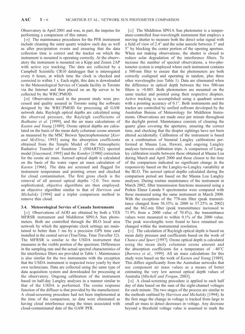
better understand the application of network measurementsto trend studies and the ability to develop a single globalclimatology from multiple networks without introducingnetwork bias, a comparison of the daily progression ofobservations for each instrument was revealing. Figure 2plots the 500-nm AOD for two periods and the 865-nmAOD for the second of these periods. The 6 and 7 July (daynumber 187 and 188) time period is for virtually cloudlessconditions (Figure 2a), while the 26 August graph (daynumber 238) (Figure 2b) illustrates the cloud removalschemes associated with the PFR and SP01A instruments.For all instruments the AOD increases dramatically at largerzenith angles with the exception of the Cimel, which doesnot report data for air mass >5. Although the optical depthsfor each of these 3 days never exceeds 0.1 at zenith angles<80�, several typical characteristics of instrument behaviorare apparent. Overall, the direct-pointing instruments trackwell, with the PFR normally reporting the largest opticaldepths and with the Cimel values being slightly less thanthe SP01A at 500 nm. The data on days 187 and 188 showthe variability in the difference between the PFR and theCimel and SP01A AOD diurnally and from day to day. Onday 238, data from the Cimel and SP01A are stable orgradually declining AOD in the late morning (238.3–238.5) while the PFR data show a gradual increase. TheCimel data also show more variability through this periodthan the other two direct sun instruments, with the SP01Ashowing the lowest variability on day 238 (the variancesbeing 8.7 � 10�5, 6.2 � 10�5, and 3.5 � 10�5 for theCimel, PFR, and SP01A, respectively). Although the AODis low between 238.45 and 238.65, the cloud-screeningalgorithms indicate significant cloud (lighter-colored, opensymbols in Figure 2b for the PFR and SP01A, whileperiods during this time are absent for the AEROCANCimel data). Abrupt changes in the AOD at 238.65 indicatethe onset of what is most probably cloud, but the earlierdata may or may not indicate cloud contamination. Thecapabilities of cloud-screening algorithms are discussed inmore detail in section 5.3.


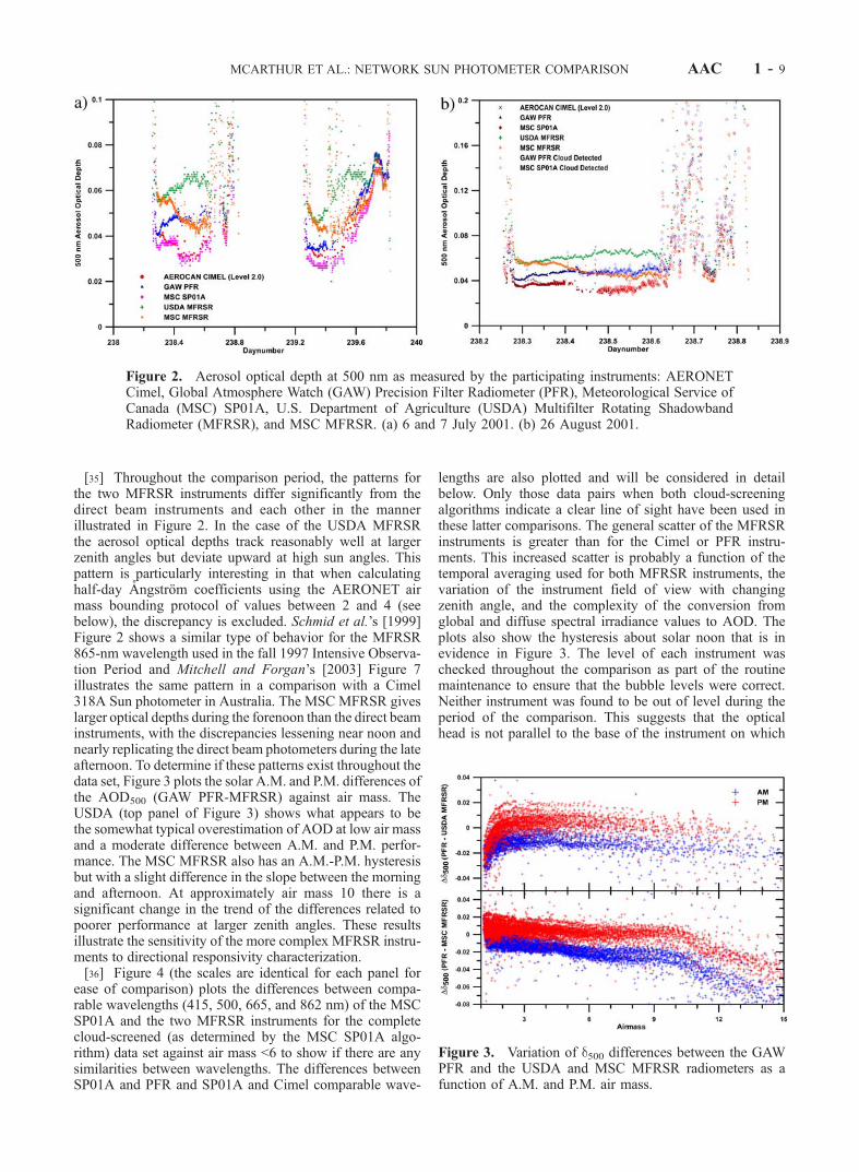
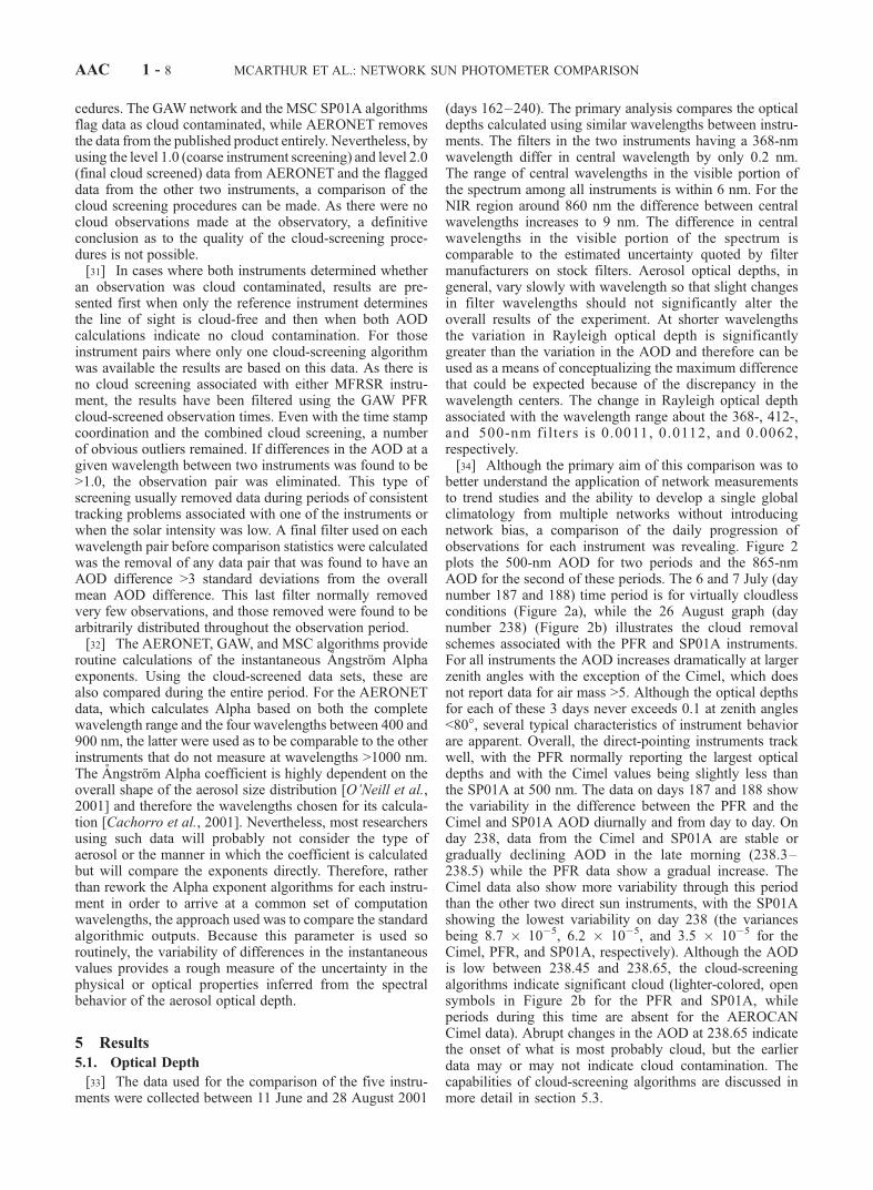
[35] Throughout the comparison period, the patterns forthe two MFRSR instruments differ significantly from thedirect beam instruments and each other in the mannerillustrated in Figure 2. In the case of the USDA MFRSRthe aerosol optical depths track reasonably well at largerzenith angles but deviate upward at high sun angles. Thispattern is particularly interesting in that when calculatinghalf-day Angstrom coefficients using the AERONET airmass bounding protocol of values between 2 and 4 (seebelow), the discrepancy is excluded. Schmid et al.’s [1999]Figure 2 shows a similar type of behavior for the MFRSR865-nm wavelength used in the fall 1997 Intensive Observa-tion Period and Mitchell and Forgan’s [2003] Figure 7illustrates the same pattern in a comparison with a Cimel318A Sun photometer in Australia. The MSC MFRSR giveslarger optical depths during the forenoon than the direct beaminstruments, with the discrepancies lessening near noon andnearly replicating the direct beam photometers during the lateafternoon. To determine if these patterns exist throughout thedata set, Figure 3 plots the solar A.M. and P.M. differences ofthe AOD500 (GAW PFR-MFRSR) against air mass. TheUSDA (top panel of Figure 3) shows what appears to bethe somewhat typical overestimation of AOD at low air massand a moderate difference between A.M. and P.M. perfor-mance. The MSC MFRSR also has an A.M.-P.M. hysteresisbut with a slight difference in the slope between the morningand afternoon. At approximately air mass 10 there is asignificant change in the trend of the differences related topoorer performance at larger zenith angles. These resultsillustrate the sensitivity of the more complex MFRSR instru-ments to directional responsivity characterization.[36] Figure 4 (the scales are identical for each panel for

ease of comparison) plots the differences between compa-rable wavelengths (415, 500, 665, and 862 nm) of the MSCSP01A and the two MFRSR instruments for the completecloud-screened (as determined by the MSC SP01A algo-rithm) data set against air mass <6 to show if there are anysimilarities between wavelengths. The differences betweenSP01A and PFR and SP01A and Cimel comparable wave-

lengths are also plotted and will be considered in detailbelow. Only those data pairs when both cloud-screeningalgorithms indicate a clear line of sight have been used inthese latter comparisons. The general scatter of the MFRSRinstruments is greater than for the Cimel or PFR instru-ments. This increased scatter is probably a function of thetemporal averaging used for both MFRSR instruments, thevariation of the instrument field of view with changingzenith angle, and the complexity of the conversion fromglobal and diffuse spectral irradiance values to AOD. Theplots also show the hysteresis about solar noon that is inevidence in Figure 3. The level of each instrument waschecked throughout the comparison as part of the routinemaintenance to ensure that the bubble levels were correct.Neither instrument was found to be out of level during theperiod of the comparison. This suggests that the opticalhead is not parallel to the base of the instrument on which

Figure 2. Aerosol optical depth at 500 nm as measured by the participating instruments: AERONETCimel, Global Atmosphere Watch (GAW) Precision Filter Radiometer (PFR), Meteorological Service ofCanada (MSC) SP01A, U.S. Department of Agriculture (USDA) Multifilter Rotating ShadowbandRadiometer (MFRSR), and MSC MFRSR. (a) 6 and 7 July 2001. (b) 26 August 2001.

Figure 3. Variation of d500 differences between the GAWPFR and the USDA and MSC MFRSR radiometers as afunction of A.M. and P.M. air mass.


the bubble level is attached. As both instruments wereoperational throughout the 2000–2001 winter, this mayindicate that regular optical leveling of this type of instru-ment is necessary because differential expansion and con-traction between the base and the optical assembly affectsthe overall radiometric alignment of the instrument. Theplacement of the level on the optical assembly of theinstrument could also reduce this type of problem. Anotherproblem associated with the MFRSR instruments is thedeterioration of the Teflon2 diffuser due to natural soilingand deterioration by the elements. Neither of these MFRSRinstruments has had an angular characterization since beingacquired in the late 1990s. These results confirm that the

characterization of the angular response be done frequently(as suggested by the manufacturer) for these types ofinstruments if accurate determinations of AOD are required.[37] The increased differences between the SP01A and

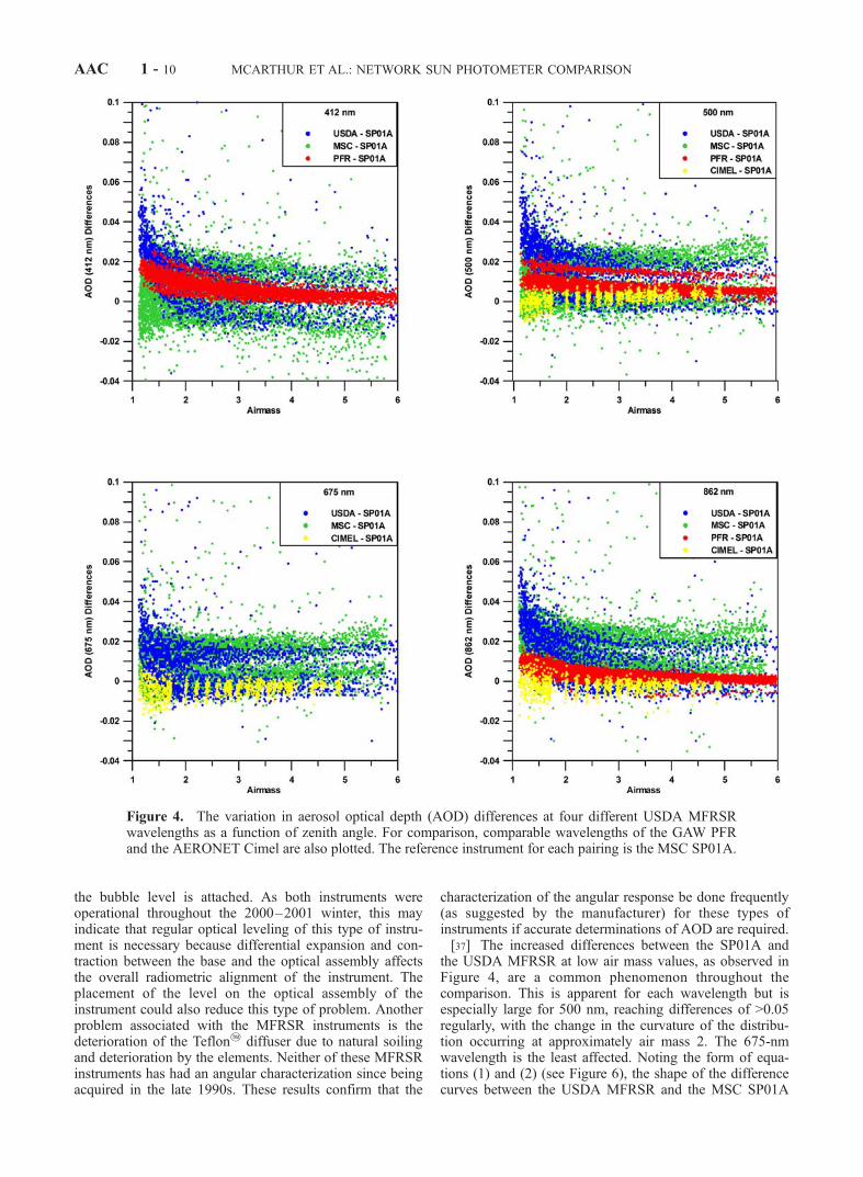
the USDA MFRSR at low air mass values, as observed inFigure 4, are a common phenomenon throughout thecomparison. This is apparent for each wavelength but isespecially large for 500 nm, reaching differences of >0.05regularly, with the change in the curvature of the distribu-tion occurring at approximately air mass 2. The 675-nmwavelength is the least affected. Noting the form of equa-tions (1) and (2) (see Figure 6), the shape of the differencecurves between the USDA MFRSR and the MSC SP01A

Figure 4. The variation in aerosol optical depth (AOD) differences at four different USDA MFRSRwavelengths as a function of zenith angle. For comparison, comparable wavelengths of the GAW PFRand the AERONET Cimel are also plotted. The reference instrument for each pairing is the MSC SP01A.


may be explained as an incorrect extraterrestrial constant(I0) for one of the two instruments. This would increase themagnitude of the differences at small air mass values (thatwould vary as (1/m) dI0/I0 but becomes nearly asymptoticas air mass increases and other error sources become morepredominant. The MSC MFRSR does not exhibit thispattern except for the 862-nm wavelength.[38] Similar changes in trend are also evident between the

SP01A and the PRF instruments for the 412- and 862-nmwavelengths and to a very small extent between the SP01Aand the Cimel at the 862-nm wavelength. In combinationwith the changes in the transmission of the 862-nm filternoted earlier, it would suggest that the calibration coeffi-cient used for the 862-nm filter of the MSC SP01A issuspect. The AOD differences between the SP01A andCimel in Figure 4 show a slight change in slope in the500-nm plot that is not found between the SP01A and thePFR. The use of a constant pressure term in the determina-tion of Rayleigh optical depth and the use of climatologicalozone optical depths yield error dependencies that resemblethese small differences. To a lesser extent, differences in theozone absorption coefficients used by each of the networkswould also account for a small portion of the bias.[39] The AOD differences between the GAW PFR and

the MSC SP01A at 500 nm, and to a lesser extent at 412nm, appear to split into two separate groups of points. Thisdivergence, however, is not related to hysteresis about solarnoon as it occurs as an offset, generally for part of or anentire day, returning to ‘‘normal’’ just as rapidly. Figure 5illustrates these two families for the 500-nm AOD differ-ences for the GAW PFR and MSC SP01A pairing. Super-imposed on the entire data set are several individual daysrepresentative of these variations. This same pattern existsbetween the AERONET Cimel and the GAW PFR, indicat-ing that the problem may be associated with the PFR. Anobvious explanation would be errors associated with the

solar tracking, but examinations of the pointing signalsrecorded within the GAW PFR data records do not showsignificant differences between the days that exhibit largerAOD differences and those within the larger family ofobservations. It should be noted that GAW PFR observa-tions that exceed the pointing criterion of 15 arc min wereeliminated from the data before this analysis. These sys-tematic differences cannot be explained at present.[40] To quantitatively describe the relationship between

the AOD for the wavelength pairs of the various instrumentsover the duration of the comparison, the root mean squaredifference (RMSD) and the mean bias difference (MBD)were computed. These can be considered as components ofthe sample variance (s2)

s2 ffi RMSD2 �MBD2; ð6Þ

where

RMSD ¼ N�1XN1

obsi � refið Þ2 !0:5

ð7Þ

MBD ¼ N�1XN1

obsi � ref ið Þ: ð8Þ

The RMSD is often associated with the nonsystematiccomponent of the differences, being sensitive to extremevalues, while the MBD describes the offset between sets ofobservations. This methodology assumes a stationarydistribution of differences, which would be expected if themethod of calculating the AOD was the same for allnetworks and the extraterrestrial coefficients were correct.However, as observed from Figure 4, this is not the case forsome of the instrument filter pairs. Therefore the resultsshould be regarded as an estimate of the differencesbetween AOD, especially between instrument pairs whereone instrument calculates AOD using equation (1) and theother uses equation (2). Figure 6 illustrates some of the airmass dependencies on AOD when using these twocalculation methods. The differences are based on a

Figure 5. Variation in the 500-nm AOD differencesbetween the GAW PFR and the MSC SP01A Sunphotometers with zenith angle.

Figure 6. Examples of the magnitude of differences inAOD associated with differences in the method ofcalculation, uncertainties in instrument calibration, andincorrect estimates of atmospheric quantities.


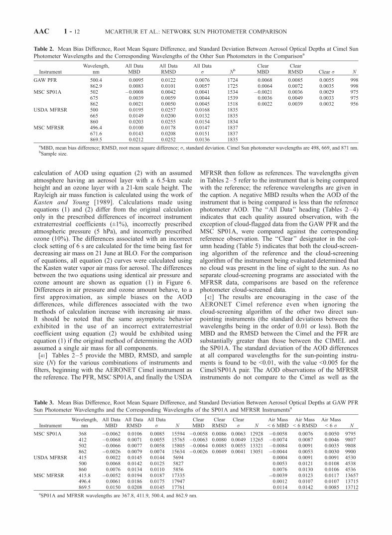
calculation of AOD using equation (2) with an assumedatmosphere having an aerosol layer with a 6.5-km scaleheight and an ozone layer with a 21-km scale height. TheRayleigh air mass function is calculated using the work ofKasten and Young [1989]. Calculations made usingequations (1) and (2) differ from the original calculationonly in the prescribed differences of incorrect instrumentextraterrestrial coefficients (±1%), incorrectly prescribedatmospheric pressure (5 hPa), and incorrectly prescribedozone (10%). The differences associated with an incorrectclock setting of 6 s are calculated for the time being fast fordecreasing air mass on 21 June at BLO. For the comparisonof equations, all equation (2) curves were calculated usingthe Kasten water vapor air mass for aerosol. The differencesbetween the two equations using identical air pressure andozone amount are shown as equation (1) in Figure 6.Differences in air pressure and ozone amount behave, to afirst approximation, as simple biases on the AODdifferences, while differences associated with the twomethods of calculation increase with increasing air mass.It should be noted that the same asymptotic behaviorexhibited in the use of an incorrect extraterrestrialcoefficient using equation (2) would be exhibited usingequation (1) if the original method of determining the AODassumed a single air mass for all components.[41] Tables 2–5 provide the MBD, RMSD, and sample

size (N) for the various combinations of instruments andfilters, beginning with the AERONET Cimel instrument asthe reference. The PFR, MSC SP01A, and finally the USDA

MFRSR then follow as references. The wavelengths givenin Tables 2–5 refer to the instrument that is being comparedwith the reference; the reference wavelengths are given inthe caption. A negative MBD results when the AOD of theinstrument that is being compared is less than the referencephotometer AOD. The ‘‘All Data’’ heading (Tables 2–4)indicates that each quality assured observation, with theexception of cloud-flagged data from the GAW PFR and theMSC SP01A, were compared against the correspondingreference observation. The ‘‘Clear’’ designator in the col-umn heading (Table 5) indicates that both the cloud-screen-ing algorithm of the reference and the cloud-screeningalgorithm of the instrument being evaluated determined thatno cloud was present in the line of sight to the sun. As noseparate cloud-screening programs are associated with theMFRSR data, comparisons are based on the referencephotometer cloud-screened data.[42] The results are encouraging in the case of the

AERONET Cimel reference even when ignoring thecloud-screening algorithm of the other two direct sun-pointing instruments (the standard deviations between thewavelengths being in the order of 0.01 or less). Both theMBD and the RMSD between the Cimel and the PFR aresubstantially greater than those between the CIMEL andthe SP01A. The standard deviation of the AOD differencesat all compared wavelengths for the sun-pointing instru-ments is found to be <0.01, with the value <0.005 for theCimel/SP01A pair. The AOD observations of the MFRSRinstruments do not compare to the Cimel as well as the

Table 2. Mean Bias Difference, Root Mean Square Difference, and Standard Deviation Between Aerosol Optical Depths at Cimel Sun

Photometer Wavelengths and the Corresponding Wavelengths of the Other Sun Photometers in the Comparisona

InstrumentWavelength,

nmAll DataMBD

All DataRMSD

All Datas Nb

ClearMBD

ClearRMSD Clear s N

GAW PFR 500.4 0.0095 0.0122 0.0076 1724 0.0068 0.0085 0.0055 998862.9 0.0083 0.0101 0.0057 1725 0.0064 0.0072 0.0035 998

MSC SP01A 502 �0.0008 0.0042 0.0041 1534 �0.0021 0.0036 0.0029 975675 0.0039 0.0059 0.0044 1539 0.0036 0.0049 0.0033 975862 0.0021 0.0050 0.0045 1518 0.0022 0.0039 0.0032 956

USDA MFRSR 500 0.0195 0.0257 0.0168 1835665 0.0149 0.0200 0.0132 1835860 0.0203 0.0255 0.0154 1834

MSC MFRSR 496.4 0.0100 0.0178 0.0147 1837671.6 0.0143 0.0208 0.0151 1837869.5 0.0212 0.0252 0.0136 1835

aMBD, mean bias difference; RMSD, root mean square difference; s, standard deviation. Cimel Sun photometer wavelengths are 498, 669, and 871 nm.bSample size.

Table 3. Mean Bias Difference, Root Mean Square Difference, and Standard Deviation Between Aerosol Optical Depths at GAW PFR

Sun Photometer Wavelengths and the Corresponding Wavelengths of the SP01A and MFRSR Instrumentsa


nmAll DataMBD

All DataRMSD

All Datas N

ClearMBD

ClearRMSD

Clears N

Air Mass< 6 MBD

Air Mass< 6 RMSD

Air Mass< 6 s N

MSC SP01A 368 �0.0062 0.0106 0.0085 15594 �0.0058 0.0086 0.0063 12928 �0.0058 0.0076 0.0050 9795412 �0.0068 0.0071 0.0055 15765 �0.0063 0.0080 0.0049 13265 �0.0074 0.0087 0.0046 9807502 �0.0066 0.0077 0.0058 15805 �0.0064 0.0085 0.0055 13321 �0.0084 0.0091 0.0035 9808862 �0.0026 0.0079 0.0074 15634 �0.0026 0.0049 0.0041 13051 �0.0044 0.0053 0.0030 9900

USDA MFRSR 415 0.0022 0.0145 0.0144 5694 0.0004 0.0091 0.0091 4530500 0.0068 0.0142 0.0125 5827 0.0053 0.0121 0.0108 4538860 0.0076 0.0134 0.0110 5856 0.0076 0.0130 0.0106 4536

MSC MFRSR 415.8 �0.0052 0.0194 0.0187 17335 �0.0039 0.0123 0.0117 13657496.4 0.0061 0.0186 0.0175 17947 0.0012 0.0107 0.0107 13715869.5 0.0150 0.0208 0.0145 17761 0.0114 0.0142 0.0085 13712

aSP01A and MFRSR wavelengths are 367.8, 411.9, 500.4, and 862.9 nm.


sun-pointing instruments, but the standard deviation of theAOD differences at all wavelengths for both instrumentsremains well <0.02. The MBD and RMSD between theCimel and the MFRSR are generally greater than twice thatcalculated for the sun-pointing instruments, possibly indi-cating the difficulty in calculating low AOD values from adifferencing methodology that also depends on averageddata. The increase in the value of both the MBD and theRMSD may be attributed to the influence of cloud duringthe duration of the averaging period. However, if this werethe sole reason for such differences, it would be expectedthat the MSC MFRSR would have performed significantlybetter than the USDA instrument because of the shorteraveraging period. The larger discrepancy between thesetwo types of instruments is probably due to the incorrectcharacterization of the directional responsivity of the instru-ments and the changing field of view with increasing airmass.[43] The MBD and the RMSD for the MSC SP01A are

found to be smaller than for the GAW PFR by approxi-mately a factor of 2 before the cloud-screening algorithmsof these two instruments are considered. When the data isexamined following application of these cloud-screeningalgorithms, the results improve, but the number of obser-vations is reduced substantially. A discussion of the dis-crepancies among cloud contamination algorithms follows.The agreement between the Cimel level 2.0 data and thecloud-screened data of the PFR and SP01A is excellent.With the exception of the Cimel/PFR 500-nm pair, the 2sdeviations are <0.01. This indicates that direct-pointinginstruments with the appropriate cloud-screening techniquescan provide data that meets the World Climate ResearchProgramme BSRN AOD accuracy criterion of 0.01 [WorldClimate Research Programme (WCRP), 1998]. However,the AOD values obtained from the two MFRSR instrumentsare in much poorer agreement, even considering the poten-

tial problems associated with cloud contamination. Thereare no cases where the RMSD is <0.01 and only one casewhere it is <0.02. The MBDs are also significantly greaterthan those associated with the direct-pointing instruments.[44] Table 3 is a comparison of the remaining instruments

against the GAW PFR. The results in the columns labeled‘‘All Data’’ in Table 3 are based on the PFR cloud-screeningalgorithm. As each of these instruments begins takingmeasurements at sunrise, the initial comparison results useall the observations that have passed through the qualityassurance procedures described earlier. The results aresimilar to those seen between the Cimel and the otherinstruments when only a single cloud-screening method isemployed. The comparison of the 368-nm filters betweenthe PFR and the SP01A show larger RMSD than at longerwavelengths, which in turn is reflected in the increasedstandard deviation over the other filters. This may indicatethe increased variability that can be expected at shorterwavelengths because of differences in the methods used incalculating Rayleigh scatter and the differences associatedwith individual pressure observations versus daily averages.The second set of columns in Table 3 (‘‘Clear’’) give theresults for all zenith angles, but only when both the SP01Aand the PFR algorithms indicate no cloud contamination.The difference in the number of observations flagged byonly one cloud-screening algorithm, but not both betweenthe PFR and the SP01A, is much smaller than in the case ofthe AERONETcomparison. However, the discrepancy in thenumber of cloud-screened observations between the variousmethods remains significant. The RMSD between the GAWPFR and MSC SP01A is smaller than between the GAWPFR and the AERONET Cimel, as expected from thecomparison of each of these instruments against the Cimel.The scatter is shown to have increased somewhat over theCimel values when all data are considered. Nevertheless,the 2s values for the 412- and 862-nm pairs remain below

Table 5. Mean Bias Difference, Root Mean Square Difference, and Standard Deviation Between Aerosol Optical Depths for the Two

MFRSR Instruments With the USDA Instrument Considered the Reference Instrumenta


nmClearMBD

ClearRMSD

Clears N

Air Mass< 6 MBD

Air Mass< 6 RMSD

Air Mass< 6 s N

MSC MFRSR 415.8 �0.0109 0.0226 0.0308 6509 �0.0068 0.0250 0.0240 5309496.4 �0.0038 0.0240 0.0237 6614 �0.0068 0.0226 0.0215 5300613.6 0.0039 0.0215 0.0212 6605 0.0016 0.0188 0.0186 5292671.6 0.0024 0.0223 0.0232 6637 0.0005 0.0189 0.0189 5297869.5 0.0050 0.0235 0.0229 6627 0.0023 0.0195 0.0193 5294

aAerosol optical depths for the MFRSR instruments are 415, 500, 610, 665, and 860 nm. The removal of cloud contaminated data was based on thecloud-screened GAW PFR observations.

Table 4. Mean Bias Difference, Root Mean Square Difference, and Standard Deviation Between Aerosol Optical Depths at MSC SP01A

Sun Photometer Wavelengths and the Corresponding Wavelengths of the MFRSR Instrumentsa


nmAll DataMBD

All DataRMSD

All Datas N

Air Mass< 6 MBD

Air Mass< 6 RMSD

Air Mass< 6 s N

USDA MFRSR 415 0.0114 0.0257 0.0231 5817 0.0122 0.0209 0.0169 4464500 0.0175 0.0251 0.0180 5880 0.0178 0.0244 0.0167 4663665 0.0101 0.0186 0.0157 5872 0.0099 0.0181 0.0152 4661860 0.0142 0.0232 0.0174 5803 0.0161 0.0240 0.0170 4604

MSC MFRSR 415.8 �0.0001 0.0345 0.0344 17961 0.0065 0.0227 0.0217 14164496.4 0.0153 0.0287 0.0243 17960 0.0119 0.0248 0.0218 14045671.6 0.0139 0.0264 0.0224 17958 0.0109 0.0242 0.0217 14162869.5 0.0200 0.0305 0.0229 17736 0.0185 0.0292 0.0226 13994

aMSC SP10A wavelengths are 412, 502, 675, and 862 nm.


0.01, while the 368- and 500-nm pairs only slightly exceedthis value.[45] The results of the two MFRSR instruments are

poorer than the direct-pointing instruments, but bothMFRSR instruments are found to have smaller MBD withrespect to the PFR than the Cimel when the evaluation isbased on the complete PFR cloud-screened data set. TheRMSDs are also found to be smaller for the USDAMFRSR. The MSC MFRSR RMSD values are marginallylarger at the 500-nm wavelength and smaller at the 869-nmwavelength. The overall standard deviation is found to besmaller for the USDA MFRSR at the two comparablewavelengths of 500 and 860 nm when compared againstthe PFR over the Cimel instrument.[46] To better compare the results obtained with the PFR

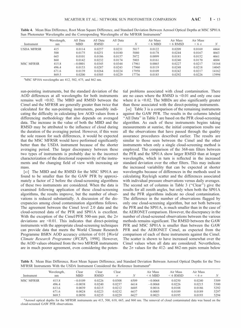
as the reference instrument with those using the Cimel asthe reference instrument, the statistics were recalculated fordata that were collected at air mass values <6. The finalfour columns of Table 3 present these results. The dataused in the comparison between the PFR and SP01A usedare those that both algorithms indicated were free of cloudcontamination. Again, the results of the comparison be-tween the direct-pointing instruments are exceptionallygood, with even the 368-nm channel having a standarddeviation of only 0.005. This implied level of opticaldepth accuracy is particularly encouraging because of theincreasingly significant role that the determination ofRayleigh optical depth plays at shorter wavelengths; avariation of 10-hPa pressure would result in a change inRayleigh optical depth at 368 nm of 0.007 that would bedirectly attributed to the AOD. While the GAW PFRinstrument includes an onboard pressure transducer, theMSC SP01A data have been calculated on the basis of adaily mean pressure, indicating that in the UV-A, pressurecorrections may be crucial in obtaining the high-qualityAOD observations required for monitoring climate vari-ability (i.e., the pressure-induced uncertainty may be amajor component of the 0.0076 value computed for 368nm in Table 3). The statistics for the MFRSR instrumentsalso improve dramatically when only values for air mass<6 are used in the analyses. The standard deviation aboutthe AOD differences between the PFR and the MFRSRinstruments are on the order of 0.01. This agreement ismuch better than between the Cimel and the MFRSRinstruments, although the difference between the direct-pointing instruments versus the rotating shadowbandinstruments still differs by a factor of two.[47] Table 4 compares the two MFRSR instruments

against the MSC SP01A. The results of the comparisonbetween the SP01A and the USDA MFRSR for air massvalues <6 are similar to the results presented between theCimel and the USDA MFRSR in Table 2. The MSCMFRSR results for air mass <6, however, are characterizedby larger RMSD values than those calculated using eitherthe Cimel or the PFR as the reference instrument.[48] Table 5 completes the comparison of AOD values by

presenting the differences between the two MFRSR instru-ments. The USDA instrument was selected as the reference.To overcome the problem associated with determiningwhether cloud was interfering with the measurements, thedata used in the comparison was matched with the times theGAW PFR cloud-screening algorithm indicated clear line-

of-sight conditions. Overall, for Air Mass <6 the standarddeviation of AOD differences between the two instrumentsis found to be only marginally larger than between theindividual MFRSR instruments and the three direct-pointinginstruments.

5.2. Angstrom Coefficients

[49] While the determination of Angstrom coefficients islinear on a log-log scale and therefore very easy to calculate,the actual optical depth spectrum is typically characterizedby nonlinear spectral curvature in the optical domain[O’Neill et al., 2001] and is sensitive to the wavelengthrange used in the determination of the coefficients[Cachorro et al., 2001]. Although these considerationswould indicate that comparing Angstrom values may beerror prone, many aerosol networks produce the a exponentas a prime indicator of the aerosol character. It has also beenused to interpolate AOD values for unknown wavelengthsin comparisons [Schmid et al., 1999] and climatologies[Holben et al., 2001], indicating its importance in aerosolobservation science. Therefore comparison between net-work values is inevitable.[50] The atmospheric aerosols encountered over the BLO

are continental in nature, well aged, and distant from pointsources. These characteristics are similar to those associatedwith the original use of Angstrom’s coefficients for deter-mining aerosol optical properties for visible wavelengths[Junge, 1963].[51] The algorithms associated with the three direct-

pointing instruments calculate the a coefficient for eachobservation. The comparability of these values providesboth an overall assessment of the similarity of the AODvalues at all wavelengths measured by each instrument andan independent measure of the confidence that can beplaced on the more complex radiative properties derivedfrom the instruments through various inversion techniques[e.g., Dubovik et al., 2000]. The MBD and RMSD betweenthe computations obtained from the three instruments aregiven in Table 6. The mean a value in Table 6 is calculatedas the average of both sets of observations and is providedto assist in assessing the quality of the agreement amongthe various instruments. The calculations followed thesame selection methodology as used in determining theAOD results. It is readily apparent that the agreementbetween the GAW PFR and the MSC SP01A is signifi-cantly better than between those instruments and theAERONET Cimel. The larger MBD and RMSD valuesassociated with the AERONET Cimel were found to besurprising considering the general good agreement betweenthe aerosol optical depths at the compared wavelengths.The calculations of MBD and RMSD were repeated usingthe AERONET reported a calculated using the full Cimelwavelength set, but no improvement was found.[52] The differences between the calculated a are a

function of the uncertainty associated with the determina-tion of a from individual instrument AODs, which isrelated to the uncertainty in the determination of the AODsand the quality of the calculation of a and the uncertaintydue to the differences in the AOD values between instru-ments. To determine the uncertainty associated with indi-vidual a, the Angstrom coefficients were recalculated sothat the standard deviation about the regression equation


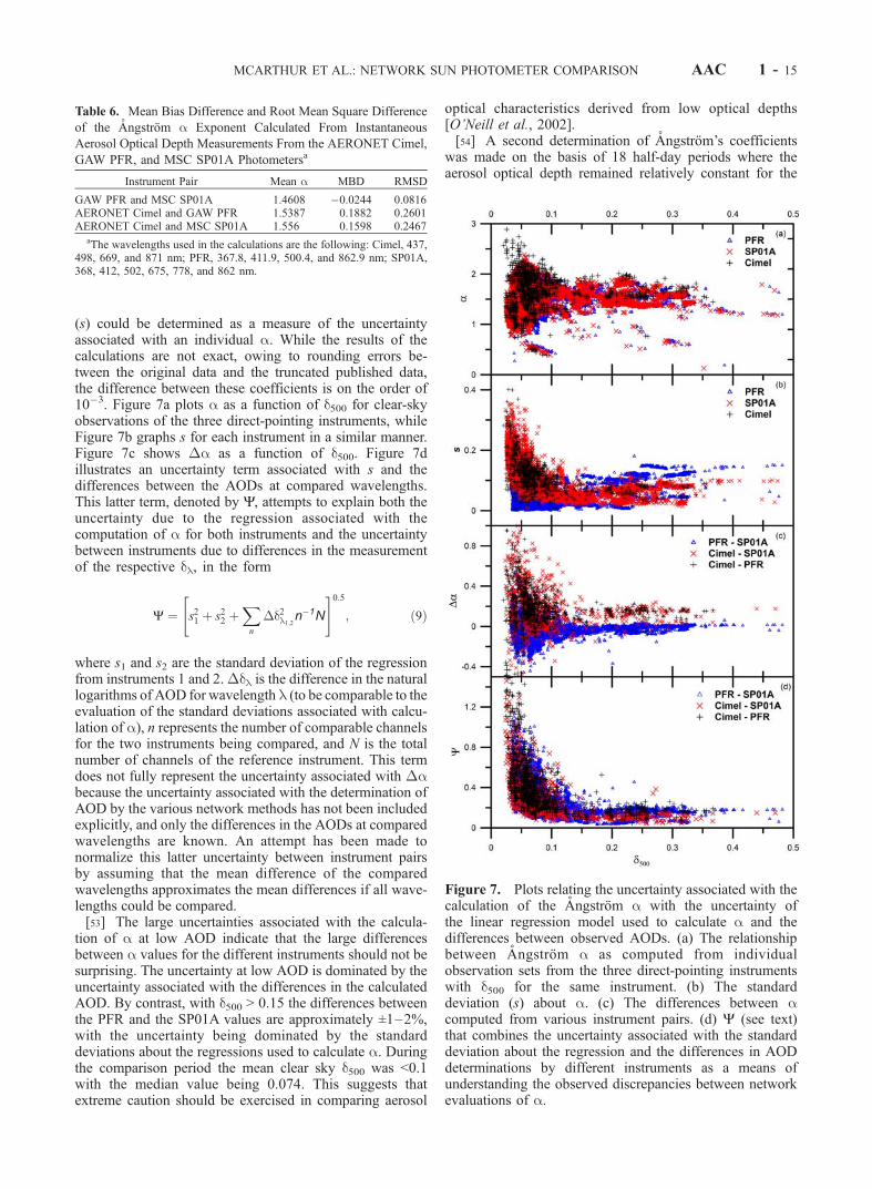
(s) could be determined as a measure of the uncertaintyassociated with an individual a. While the results of thecalculations are not exact, owing to rounding errors be-tween the original data and the truncated published data,the difference between these coefficients is on the order of10�3. Figure 7a plots a as a function of d500 for clear-skyobservations of the three direct-pointing instruments, whileFigure 7b graphs s for each instrument in a similar manner.Figure 7c shows �a as a function of d500. Figure 7dillustrates an uncertainty term associated with s and thedifferences between the AODs at compared wavelengths.This latter term, denoted by Y, attempts to explain both theuncertainty due to the regression associated with thecomputation of a for both instruments and the uncertaintybetween instruments due to differences in the measurementof the respective dl, in the form

Y ¼ s21 þ s22 þXn

�d2l1;2n�1N

" #0:5; ð9Þ

where s1 and s2 are the standard deviation of the regressionfrom instruments 1 and 2.�dl is the difference in the naturallogarithms of AOD for wavelength l (to be comparable to theevaluation of the standard deviations associated with calcu-lation of a), n represents the number of comparable channelsfor the two instruments being compared, and N is the totalnumber of channels of the reference instrument. This termdoes not fully represent the uncertainty associated with �abecause the uncertainty associated with the determination ofAOD by the various network methods has not been includedexplicitly, and only the differences in the AODs at comparedwavelengths are known. An attempt has been made tonormalize this latter uncertainty between instrument pairsby assuming that the mean difference of the comparedwavelengths approximates the mean differences if all wave-lengths could be compared.[53] The large uncertainties associated with the calcula-

tion of a at low AOD indicate that the large differencesbetween a values for the different instruments should not besurprising. The uncertainty at low AOD is dominated by theuncertainty associated with the differences in the calculatedAOD. By contrast, with d500 > 0.15 the differences betweenthe PFR and the SP01A values are approximately ±1–2%,with the uncertainty being dominated by the standarddeviations about the regressions used to calculate a. Duringthe comparison period the mean clear sky d500 was <0.1with the median value being 0.074. This suggests thatextreme caution should be exercised in comparing aerosol

optical characteristics derived from low optical depths[O’Neill et al., 2002].[54] A second determination of Angstrom’s coefficients

was made on the basis of 18 half-day periods where theaerosol optical depth remained relatively constant for the

Table 6. Mean Bias Difference and Root Mean Square Difference

of the Angstrom a Exponent Calculated From Instantaneous

Aerosol Optical Depth Measurements From the AERONET Cimel,

GAW PFR, and MSC SP01A Photometersa

Instrument Pair Mean a MBD RMSD

GAW PFR and MSC SP01A 1.4608 �0.0244 0.0816AERONET Cimel and GAW PFR 1.5387 0.1882 0.2601AERONET Cimel and MSC SP01A 1.556 0.1598 0.2467

aThe wavelengths used in the calculations are the following: Cimel, 437,498, 669, and 871 nm; PFR, 367.8, 411.9, 500.4, and 862.9 nm; SP01A,368, 412, 502, 675, 778, and 862 nm.

Figure 7. Plots relating the uncertainty associated with thecalculation of the Angstrom a with the uncertainty ofthe linear regression model used to calculate a and thedifferences between observed AODs. (a) The relationshipbetween Angstrom a as computed from individualobservation sets from the three direct-pointing instrumentswith d500 for the same instrument. (b) The standarddeviation (s) about a. (c) The differences between acomputed from various instrument pairs. (d) Y (see text)that combines the uncertainty associated with the standarddeviation about the regression and the differences in AODdeterminations by different instruments as a means ofunderstanding the observed discrepancies between networkevaluations of a.


entire period. The mean AOD for each wavelength from allfive instruments was determined over the air mass range of2–6. These data were then used to obtain the a coefficientsfor the period (Figure 8). The results confirm the discrep-ancies between the AERONET Cimel, GAW PFR, andMSC SP01A results reported above. In all cases the adetermined from the AERONET Cimel data is larger thanthose calculated using data from the other photometers inthe comparison. The MFRSR results in this graph indicatethat the MSC instrument significantly underestimates a forall periods. This corresponds to the significant and generallyincreasing bias with wavelength between the MSC instru-ment and the direct-pointing instruments (Tables 2–4) thatis indicative of a spectral flattening compared to the otherinstruments. The USDA MFRSR results suggest a solarposition dependency, the morning values being smaller thanthe a calculated from both the GAW PFR and MSC SP01Adata, with the afternoon values being greater or nearlyequal. The rapid increase in AOD near midday exhibitedby this instrument (Figure 2) occurs at air mass values <2and so does not enter into these calculations. The largerange in a seen in Figure 8 indicates the magnitude of theuncertainties that may exist between Angstrom coefficientsderived from the various network instruments. These resultswould indicate that using such parameters, as part of aglobal climatology, should be discouraged at present.

5.3. Cloud Screening Algorithms

[55] The AOD observations that have been used in thiscomparison are based on automatic cloud-screening techni-ques. The discrepancies in the number of observations thatwere removed because of apparent cloud contamination bythe different quality assurance procedures were found to begreater than anticipated. Therefore a brief analysis has beenundertaken to determine the differences between themethods. Unfortunately, continuous cloud observations arenot made at present at the BLO, so no definitive conclusioncan be made as to the overall quality of the screeningalgorithms. However, it is believed that comparing thedifferences between the instruments will encourage moreeffort in testing the present approaches and the developmentof new algorithms.[56] The AERONET data are both prescreened for data

quality at the time of the observation and screened during anautomatic quality control procedure. Neither the GAW PFRnor the MSC SP01A data are prescreened, but both useautomatic quality assurance procedures that indicate whethercloud is present during the observation. In both cases theflagged data remain as part of the data set. Details ofthe screening procedures are given in section 3. Before thecloud-screening algorithms were compared, any data asso-ciated with instrument malfunctions or pointing errors wereremoved. For the AERONET data it was assumed that allobservations removed between level 1.0, unscreened dataand level 1.5 cloud-screened data were due only to the cloud-screening process and that the difference in the number ofobservations between level 1.5 data and the level 2.0 dataused in the comparison were for reasons other than cloudcontamination. The slight differences in the times ofmatched observations are not expected to alter the overallresults of the comparison. It is recognized that on days whereobservations were made during conditions of scattered

clouds, individual observations among the three might showdifferences, but it is expected that the randomness of thisprocess will not result in significantly different numbers ofscreened observations overall.[57] Between 11 June and 28 August the AERONET

Cimel reported 2782 valid level 1.0 observations (level 1.0less the difference between level 1.5 and level 2.0 obser-vations), of which 67% were determined to be cloud-freeby the AERONET cloud-screening algorithm (Table 7).During the same period the GAW algorithm screened out69% of its observations as cloud contaminated and theMSC algorithm screened out 49% of all observations ascontaminated by cloud. AERONET employs a ‘‘coarsetriplet rejection’’ criterion on three observations taken 30s apart over a 1-min period, and data not passing the testare not transmitted. As the number of AERONET Cimelobservations not reported because of this is unknown, thepre-cloud-screened data from the GAW and MSC data setswere paired with the valid Cimel level 1.0 data to permit asimilar reference for determining the percentage of cloud-free data. In contrast to the general percentages of datarejected as cloud contaminated, the GAW algorithm appliedto the PFR observations obtained at the same time as theAERONET Cimel level 1.0 observations, determined only51% to be cloud-free, 16% less than the AERONETalgorithm resolved. Not only is there a significant differ-ence in the number of observations that were determined tobe uncontaminated by cloud, but there is also a discrepancybetween which observations were determined to be cloudcontaminated. As the comparison between the AERONETalgorithm and the algorithms used for the PFR and SP01Ais based on the level 1.0 and above data, the issue of offsettime is eliminated because observations were obtainedwithin the period of the Cimel triplet observation. Usingthe GAW rejection criteria, 42% of the AERONET level 2.0data would have been determined to be cloud contaminated.This does not imply, however, that the GAW algorithm issimply more conservative in its determination of cloudlessconditions. Approximately 12% of the Cimel level 1.0temporally matched data were determined to be cloud

Figure 8. Comparison of the Angstrom Alpha exponentcalculated from half-day mean AODs calculated by the fivenetwork instruments.


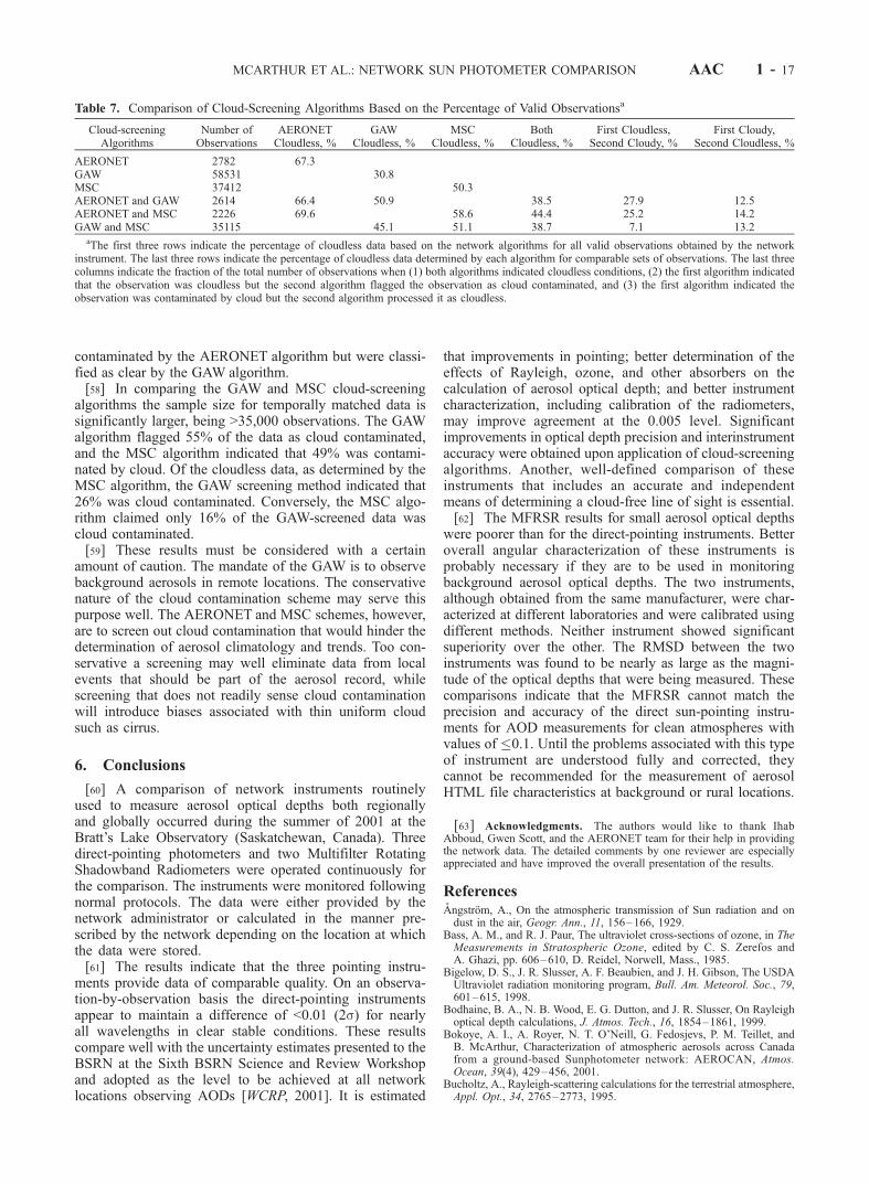
contaminated by the AERONET algorithm but were classi-fied as clear by the GAW algorithm.[58] In comparing the GAW and MSC cloud-screening

algorithms the sample size for temporally matched data issignificantly larger, being >35,000 observations. The GAWalgorithm flagged 55% of the data as cloud contaminated,and the MSC algorithm indicated that 49% was contami-nated by cloud. Of the cloudless data, as determined by theMSC algorithm, the GAW screening method indicated that26% was cloud contaminated. Conversely, the MSC algo-rithm claimed only 16% of the GAW-screened data wascloud contaminated.[59] These results must be considered with a certain

amount of caution. The mandate of the GAW is to observebackground aerosols in remote locations. The conservativenature of the cloud contamination scheme may serve thispurpose well. The AERONET and MSC schemes, however,are to screen out cloud contamination that would hinder thedetermination of aerosol climatology and trends. Too con-servative a screening may well eliminate data from localevents that should be part of the aerosol record, whilescreening that does not readily sense cloud contaminationwill introduce biases associated with thin uniform cloudsuch as cirrus.

6. Conclusions

[60] A comparison of network instruments routinelyused to measure aerosol optical depths both regionallyand globally occurred during the summer of 2001 at theBratt’s Lake Observatory (Saskatchewan, Canada). Threedirect-pointing photometers and two Multifilter RotatingShadowband Radiometers were operated continuously forthe comparison. The instruments were monitored followingnormal protocols. The data were either provided by thenetwork administrator or calculated in the manner pre-scribed by the network depending on the location at whichthe data were stored.[61] The results indicate that the three pointing instru-

ments provide data of comparable quality. On an observa-tion-by-observation basis the direct-pointing instrumentsappear to maintain a difference of <0.01 (2s) for nearlyall wavelengths in clear stable conditions. These resultscompare well with the uncertainty estimates presented to theBSRN at the Sixth BSRN Science and Review Workshopand adopted as the level to be achieved at all networklocations observing AODs [WCRP, 2001]. It is estimated

that improvements in pointing; better determination of theeffects of Rayleigh, ozone, and other absorbers on thecalculation of aerosol optical depth; and better instrumentcharacterization, including calibration of the radiometers,may improve agreement at the 0.005 level. Significantimprovements in optical depth precision and interinstrumentaccuracy were obtained upon application of cloud-screeningalgorithms. Another, well-defined comparison of theseinstruments that includes an accurate and independentmeans of determining a cloud-free line of sight is essential.[62] The MFRSR results for small aerosol optical depths

were poorer than for the direct-pointing instruments. Betteroverall angular characterization of these instruments isprobably necessary if they are to be used in monitoringbackground aerosol optical depths. The two instruments,although obtained from the same manufacturer, were char-acterized at different laboratories and were calibrated usingdifferent methods. Neither instrument showed significantsuperiority over the other. The RMSD between the twoinstruments was found to be nearly as large as the magni-tude of the optical depths that were being measured. Thesecomparisons indicate that the MFRSR cannot match theprecision and accuracy of the direct sun-pointing instru-ments for AOD measurements for clean atmospheres withvalues of �0.1. Until the problems associated with this typeof instrument are understood fully and corrected, theycannot be recommended for the measurement of aerosolHTML file characteristics at background or rural locations.

[63] Acknowledgments. The authors would like to thank IhabAbboud, Gwen Scott, and the AERONET team for their help in providingthe network data. The detailed comments by one reviewer are especiallyappreciated and have improved the overall presentation of the results.

ReferencesAngstrom, A., On the atmospheric transmission of Sun radiation and ondust in the air, Geogr. Ann., 11, 156–166, 1929.

Bass, A. M., and R. J. Paur, The ultraviolet cross-sections of ozone, in TheMeasurements in Stratospheric Ozone, edited by C. S. Zerefos andA. Ghazi, pp. 606–610, D. Reidel, Norwell, Mass., 1985.

Bigelow, D. S., J. R. Slusser, A. F. Beaubien, and J. H. Gibson, The USDAUltraviolet radiation monitoring program, Bull. Am. Meteorol. Soc., 79,601–615, 1998.

Bodhaine, B. A., N. B. Wood, E. G. Dutton, and J. R. Slusser, On Rayleighoptical depth calculations, J. Atmos. Tech., 16, 1854–1861, 1999.

Bokoye, A. I., A. Royer, N. T. O’Neill, G. Fedosjevs, P. M. Teillet, andB. McArthur, Characterization of atmospheric aerosols across Canadafrom a ground-based Sunphotometer network: AEROCAN, Atmos.Ocean, 39(4), 429–456, 2001.

Bucholtz, A., Rayleigh-scattering calculations for the terrestrial atmosphere,Appl. Opt., 34, 2765–2773, 1995.

Table 7. Comparison of Cloud-Screening Algorithms Based on the Percentage of Valid Observationsa

Cloud-screeningAlgorithms

Number ofObservations

AERONETCloudless, %

GAWCloudless, %

MSCCloudless, %

BothCloudless, %

First Cloudless,Second Cloudy, %

First Cloudy,Second Cloudless, %

AERONET 2782 67.3GAW 58531 30.8MSC 37412 50.3AERONET and GAW 2614 66.4 50.9 38.5 27.9 12.5AERONET and MSC 2226 69.6 58.6 44.4 25.2 14.2GAW and MSC 35115 45.1 51.1 38.7 7.1 13.2

aThe first three rows indicate the percentage of cloudless data based on the network algorithms for all valid observations obtained by the networkinstrument. The last three rows indicate the percentage of cloudless data determined by each algorithm for comparable sets of observations. The last threecolumns indicate the fraction of the total number of observations when (1) both algorithms indicated cloudless conditions, (2) the first algorithm indicatedthat the observation was cloudless but the second algorithm flagged the observation as cloud contaminated, and (3) the first algorithm indicated theobservation was contaminated by cloud but the second algorithm processed it as cloudless.


Burrows, J. P., A. Richter, A. Dern, B. Deters, S. Himmelmann, S. Voight,and J. Orphal, Atmospheric remote-sensing reference data from GOME:Part 2. Temperature dependent absorption cross-sections of O3 in the231–794 nm range, J. Quant. Spectrosc. Radiat. Transfer, 61, 509–517, 1999.

Cachorro, V. E., R. Vergaz, and A. M. de Frutos, A quantitative comparisonof a-A turbidity parameter retrieved in different spectral ranges based onspectroradiometer solar radiation measurements, Atmos. Environ., 35,5117–5124, 2001.

Chance, K., and R. J. D. Spurr, Ring effect studies: Rayleigh scattering,including molecular parameters for rotational Raman scattering, and theFraunhofer spectrum, Appl. Opt., 36, 5224–5230, 1997.

Dubovik, O., A. Smirnov, B. N. Holben, M. D. King, Y. J. Kaufman, T. F.Eck, and I. Slutsker, Accuracy assessments of aerosol optical propertiesretrieved from Aerosol Robotic Network (AERONET) Sun and skyradiance measurements, J. Geophys. Res., 105, 9791–9806, 2000.

Eck, T. F., B. N. Holben, J. S. Reid, O. Dubovik, A. Smirnov, N. T. O’Neill,I. Slutsker, and S. Kinne, Wavelength dependence of the optical depth ofbiomass burning, urban, and desert dust aerosols, J. Geophys. Res., 104,31,333–31,349, 1999.

Fedosejevs, G., N. T. O’Neill, A. Royer, P. M. Teillet, A. I. Bokoye, andB. McArthur, Aerosol optical depth for atmospheric correction ofAVHRR composite data, Can. J. Remote Sens., 26, 273–284, 2000.

Forgan, B. W., Sun photometer calibration by the ratio-Langley method, inBaseline Atmospheric Program (Australia) 1986, edited by B. W. Forganand P. J. Fraser, pp. 22–26, Bur. of Meteorol., Melbourne, Australia,1988.

Forgan, B. W., General method for calibration sun photometers, Appl. Opt.,33, 4841–4850, 1994.

Gueymard, C., SMARTS2, a simple model of the atmospheric radiativetransfer of sunshine: Algorithms and performance assessment, Rep.FSEC-PF-270-95, Fla. Sol. Energy Cent., Cocoa, Florida, 1995.

Harrison, L., and J. Michalsky, Objective algorithms for the retrieval ofoptical depths from ground-based measurements, Appl. Opt., 33, 5126–5132, 1994.

Harrison, L., J. Michalsky, and J. Berndt, Automated multifilter rotatingshadow-band radiometer: An instrument for optical depth and radiationmeasurements, Appl. Opt., 33, 5118–5125, 1994.

Holben, B. N., et al., AERONET—A federated instrument network anddata archive for aerosol characterization, Remote Sens. Environ., 66,1–16, 1998.

Holben, B. N., et al., An emerging ground-based aerosol Climatology:Aerosol optical depth from AERONET, J. Geophys. Res., 106,12,067–12,097, 2001.

Ingold, T., C. Matzler, N. Kampfer, and A. Heimo, Aerosol optical depthmeasurements by means of a Sun photometer network in Switzerland,J. Geophys. Res., 106, 27,537–27,554, 2001.

Junge, C. E., Air Chemistry and Radioactivity, Academic, San Diego,Calif., 1963.

Kasten, F., A new talbe and approximation formula for relative optical airmass, Arch. Meteorol. Geophys. Bioklimatol., Ser. B, 14, 206–223, 1966.

Kasten, F., and A. T. Young, Revised optical air mass tables and approx-imation formula, Appl. Opt., 28, 4735–4738, 1989.

Kerr, J. B., and C. T. McElroy, Evidence for large upward trends of ultra-violet-B radiation linked to ozone depletion, Science, 262, 1032–1034,1993.

Komhyr, W. D., Operations Handbook—Ozone observations with aDobson Spectrometer, WMO Global Ozone Res. and Monit. Proj.No. 6., Natl. Ocean. and Atmos. Admin., Environ. Res. Lab., Air Resour.Lab., Boulder, Colo., 1980.

London, J., R. D. Bojkov, S. Oltmans, and J. I. Kelley, Atlas of the GlobalDistribution of Total Ozone July 1957–June 1967, NCAR Tech. Note133+STR, 276 pp., Natl. Cent. for Atmos. Res., Boulder, Colo., 1976.

Michalsky, J. J., R. Perez, and R. Stewart, Design and development of arotating shadowband radiometer solar radiation/daylight network, Sol.Energy, 6, 577–581, 1988.

Michalsky, J. J., J. A. Schlemmer, W. E. Berkheiser, J. L. Berndt, L. C.Harrison, N. S. Laulainen, N. R. Larson, and J. C. Barnard, Multiyearmeasurements of aerosol optical depth in the Atmospheric RadiationMeasurement and Quantitative Links programs, J. Geophys. Res., 106,12,099–12,107, 2001.

Mitchell, R. M., and B. W. Forgan, Aerosol measurement in the AustralianOutback: Intercomparison of Sun photometers, J. Atmos. Oceanic Tech-nol., 20, 54–66, 2003.

O’Neill, N. T., T. F. Eck, B. N. Holben, A. Smirnov, O. Dubovik, andA. Royer, Bi-modal size distribution influences on the variation of Ang-strom derivatives in spectral and optical depth space, J. Geophys. Res.,106, 9787–9806, 2001.

O’Neill, N. T., T. F. Eck, B. N. Holben, A. Smirnov, A. Royer, and Z. Li,Optical properties of boreal forest fire smoke derived from Sun photo-metry, J. Geophys. Res., 107(D11), 4125, doi:10.1029/2001JD000877,2002.

Schmid, B., J. Michalsky, R. Halthorne, M. Beauharnois, L. Harrison,J. Livingston, P. Russell, B. Holben, T. Eck, and A. Smirnov, Comparisonof aerosol optical depth from four solar radiometers during the fall 1997ARM intensive observation period, Geophys. Res. Lett., 26(17), 2725–2728, 1999.

Shettle, E. P., and S. M. Anderson, New visible and near IR ozone absorp-tion cross-sections for MODTRAN, in Proc. 17th Annu. Rev. Conf.Atmos. Trans. Models, 8–9 June 1994, PL-TR-95-2060 Special Reports,no. 274, edited by G. P. Anderson, R. H. Picard, and J. H. Chetwind, pp.335–350, Phillips Lab., Directorate of Geophys., Hanscom Air ForceBase, Mass., 1995.

Smirnov, A., B. N. Holben, T. F. Eck, O. Dubovik, and I. Slutsker, Cloud-screening and quality control algorithms for the AERONET database,Remote Sens. Environ., 73, 337–349, 2000.

Stephens, G. L., Remote Sensing of the Lower Atmosphere, Oxford Univ.Press, New York, 1994.

Vigroux, E., Contribution a l’etude experimentale de l’absorption de l’ox-one, Ann. Phys., 8, 709, 1953.

Wehrli, C., Calibrations of filter radiometers for determination of atmo-spheric optical depth, Metrologia, 37, 419–422, 2000.

World Climate Research Programme (WCRP), Report of the fifth BSRNscience and review workshop, World Climate Research Programme Base-line Surface Radiation Network (BSRN), Budapest, Hungary, 18–22May 1998, WCRP Informal Rep. 10/1998, Geneva, Switzerland, 1998.

WCRP, Report of the sixth BSRN science and review workshop, WorldClimate Research Programme Baseline Surface Radiation Network(BSRN), Melbourne, Australia, 1–5 May 2000, WCRP Informal Rep.17/2001, Geneva, Switzerland, 2001.

��D. H. Halliwell and O. J. Niebergall, Bratt’s Lake Observatory,

Meteorological Service of Canada, P.O. Box 160, Wilcox, Saskatchewan,Canada, S0G 5E0. ([email protected]; [email protected])L. J. B. McArthur, Meteorological Service of Canada, 4905 Dufferin

Street, Downsview, Ontario, Canada M3H 5T4. ([email protected])N. T. O’Neill, Le Centre d’applications et de recherches en teledetection,

Univeristy of Sherbrooke, Sherbrooke, Quebec, Canada J1K 2R1. ([email protected])J. R. Slusser, U.S. Department of Agriculture UV-B Monitoring and

Research Program, Colorado State University, Fort Collins, CO 80523-1499, USA. ([email protected])C. Wehrli, Physikalisch-Meteorologisches Observatorium/World Radia-

tion Centre, 33, CH-7260 Davos, Switzerland. ([email protected])


Field comparison of network Sun photometers · Systems (YES) Multifilter Rotating Shadowband...

Documents

Transcript of Field comparison of network Sun photometers · Systems (YES) Multifilter Rotating Shadowband...