Field Application of a Permeable Reactive Barrier for Treatment of Arsenic in Ground Water

Office of Research and Development National Risk Management Research Laboratory, Ada, Oklahoma 74820

EPA 600/R-08/093 | September 2008 | www.epa.gov/ada

Field Application of a Permeable Reactive Barrier for Treatment of Arsenic in Ground Water

Richard T. Wilkin, Steven D. Acree, Douglas G. Beak, Randall R. Ross, Tony R. Lee, and Cindy J. Paul Ground Water and Ecosystems Restoration Division

Office of Research and Development National Risk Management Research Laboratory, Ada, Oklahoma 74820

Notice

The U.S. Environmental Protection Agency through its Office of Research and Development funded the research described here. It has been subjected to the Agency’s peer and administrative review and has been approved for publication as an EPA document. Mention of trade names or commercial products does not constitute endorsement or recommendation for use.

All research projects making conclusions or recommendations based on en­vironmentally related measurements and funded by the Environmental Protection Agency are required to participate in the Agency Quality Assurance Program. This project was conducted under an approved Quality Assurance Project Plan. The procedures specified in this plan were used without exception. Information on the plan and documentation of the quality assurance activities and results are available from the Principal Investigator.

ii

Robert W. Puls, Acting Director Ground Water and Ecosystems Restoration Division National Risk Management Research Laboratory

Foreword

The U.S. Environmental Protection Agency (EPA) is charged by Congress with protecting the Nation’s land, air, and water resources. Under a mandate of national environmental laws, the Agency strives to formulate and implement actions leading to a compatible balance between human activities and the ability of natural systems to support and nurture life. To meet this mandate, EPA’s research program is providing data and technical support for solving environmental problems today and building a science knowledge base necessary to manage our ecological resources wisely, understand how pollutants affect our health, and prevent or reduce environmental risks in the future.

The National Risk Management Research Laboratory (NRMRL) is the Agency’s center for investigation of technological and management approaches for preventing and reducing risks from pollution that threatens human health and the environment. The focus of the Laboratory’s research program is on methods and their cost-effectiveness for prevention and control of pollution to air, land, water, and subsurface resources; protection of water quality in public water systems; remediation of contaminated sites, sediments and ground water; prevention and control of indoor air pollution; and restoration of ecosystems. NRMRL collaborates with both public and private sector partners to foster technologies that reduce the cost of compliance and to anticipate emerging problems. NRMRL’s research provides solutions to environmental problems by: developing and promoting technologies that protect and improve the environment; advancing scientific and engineering information to support regulatory and policy decisions; and providing the technical support and information transfer to ensure implementation of environmental regulations and strategies at the national, state, and community levels.

This publication has been produced as part of the Laboratory’s strategic long-term research plan. It is published and made available by EPA’s Office of Research and Development (ORD) to assist the user community and to link researchers with their clients. Arsenic is a common ground-water contaminant at hazardous waste sites. The purpose of this document is to provide a hydrologic and geochemical analysis of a pilot-scale Permeable Reactive Barrier (PRB) installed to treat ground water contaminated with arsenic. This report will fill a need for a readily available source of information for site managers and others who are faced with the need to remediate ground water contaminated with inorganic compounds and are considering the use of this cost-effective technology. The information provided in this document will be of use to stakeholders such as state and federal regulators, Native American tribes, consultants, contractors, and other interested parties.

iii

ContentsContents

Notice . . . . . . . . . . . . . . . . . . . . . . . . . . . . . . . . . . . . . . . . . . . . . . . . . . . . . . . . . . . . . . . . . . . . . . . . . . . . . ii Foreword . . . . . . . . . . . . . . . . . . . . . . . . . . . . . . . . . . . . . . . . . . . . . . . . . . . . . . . . . . . . . . . . . . . . . . . . . . . iii Figures . . . . . . . . . . . . . . . . . . . . . . . . . . . . . . . . . . . . . . . . . . . . . . . . . . . . . . . . . . . . . . . . . . . . . . . . . . . . . vi Tables . . . . . . . . . . . . . . . . . . . . . . . . . . . . . . . . . . . . . . . . . . . . . . . . . . . . . . . . . . . . . . . . . . . . . . . . . . . . . ix

Acknowledgments . . . . . . . . . . . . . . . . . . . . . . . . . . . . . . . . . . . . . . . . . . . . . . . . . . . . . . . . . . . . . . . . . . . . x

Abstract . . . . . . . . . . . . . . . . . . . . . . . . . . . . . . . . . . . . . . . . . . . . . . . . . . . . . . . . . . . . . . . . . . . . . . . . . . . . xi1.0 Introduction . . . . . . . . . . . . . . . . . . . . . . . . . . . . . . . . . . . . . . . . . . . . . . . . . . . . . . . . . . . . . . . . . . . . 1

2.0 Background . . . . . . . . . . . . . . . . . . . . . . . . . . . . . . . . . . . . . . . . . . . . . . . . . . . . . . . . . . . . . . . . . . . . 2 Arsenic in ground water . . . . . . . . . . . . . . . . . . . . . . . . . . . . . . . . . . . . . . . . . . . . . . . . . . . . . . . . . 2 Arsenic removal from water by zerovalent iron . . . . . . . . . . . . . . . . . . . . . . . . . . . . . . . . . . . . . . 3

3.0 Site Background . . . . . . . . . . . . . . . . . . . . . . . . . . . . . . . . . . . . . . . . . . . . . . . . . . . . . . . . . . . . . . . . 4

4.0 PRB Installation . . . . . . . . . . . . . . . . . . . . . . . . . . . . . . . . . . . . . . . . . . . . . . . . . . . . . . . . . . . . . . . . 6 Construction details . . . . . . . . . . . . . . . . . . . . . . . . . . . . . . . . . . . . . . . . . . . . . . . . . . . . . . . . . . . . 6

5.0 Methodology . . . . . . . . . . . . . . . . . . . . . . . . . . . . . . . . . . . . . . . . . . . . . . . . . . . . . . . . . . . . . . . . . . . 8 Well network . . . . . . . . . . . . . . . . . . . . . . . . . . . . . . . . . . . . . . . . . . . . . . . . . . . . . . . . . . . . . . . . . 8 Water sampling and analysis . . . . . . . . . . . . . . . . . . . . . . . . . . . . . . . . . . . . . . . . . . . . . . . . . . . . . 9 Arsenic speciation modeling . . . . . . . . . . . . . . . . . . . . . . . . . . . . . . . . . . . . . . . . . . . . . . . . . . . . . 10 Core sampling and analysis . . . . . . . . . . . . . . . . . . . . . . . . . . . . . . . . . . . . . . . . . . . . . . . . . . . . . . 11 X-ray spectroscopy . . . . . . . . . . . . . . . . . . . . . . . . . . . . . . . . . . . . . . . . . . . . . . . . . . . . . . . . . . . . 12 Hydrologic methods . . . . . . . . . . . . . . . . . . . . . . . . . . . . . . . . . . . . . . . . . . . . . . . . . . . . . . . . . . . . 13

6.0 Results and Discussion . . . . . . . . . . . . . . . . . . . . . . . . . . . . . . . . . . . . . . . . . . . . . . . . . . . . . . . . . . . 17 Ground-water geochemistry . . . . . . . . . . . . . . . . . . . . . . . . . . . . . . . . . . . . . . . . . . . . . . . . . . . . . 17 PRB behavior . . . . . . . . . . . . . . . . . . . . . . . . . . . . . . . . . . . . . . . . . . . . . . . . . . . . . . . . . . . . . . . . . 22 Hydraulic investigation . . . . . . . . . . . . . . . . . . . . . . . . . . . . . . . . . . . . . . . . . . . . . . . . . . . . . . . . . 26 Flux evaluations . . . . . . . . . . . . . . . . . . . . . . . . . . . . . . . . . . . . . . . . . . . . . . . . . . . . . . . . . . . . . . . 34 PRB performance . . . . . . . . . . . . . . . . . . . . . . . . . . . . . . . . . . . . . . . . . . . . . . . . . . . . . . . . . . . . . . 35 Scanning electron microscopy . . . . . . . . . . . . . . . . . . . . . . . . . . . . . . . . . . . . . . . . . . . . . . . . . . . . 38 X-ray absorption spectroscopy . . . . . . . . . . . . . . . . . . . . . . . . . . . . . . . . . . . . . . . . . . . . . . . . . . . 40

7.0 Future Study Improvements . . . . . . . . . . . . . . . . . . . . . . . . . . . . . . . . . . . . . . . . . . . . . . . . . . . . . . . 45

8.0 Summary and Relevance to Other Sites . . . . . . . . . . . . . . . . . . . . . . . . . . . . . . . . . . . . . . . . . . . . . . 46

9.0 References . . . . . . . . . . . . . . . . . . . . . . . . . . . . . . . . . . . . . . . . . . . . . . . . . . . . . . . . . . . . . . . . . . . . . 48

Appendices . . . . . . . . . . . . . . . . . . . . . . . . . . . . . . . . . . . . . . . . . . . . . . . . . . . . . . . . . . . . . . . . . . . . . . . . . 52 Appendix A . . . . . . . . . . . . . . . . . . . . . . . . . . . . . . . . . . . . . . . . . . . . . . . . . . . . . . . . . . . . . . . . . . . . . . 52 Appendix B . . . . . . . . . . . . . . . . . . . . . . . . . . . . . . . . . . . . . . . . . . . . . . . . . . . . . . . . . . . . . . . . . . . . . . 54 Appendix C . . . . . . . . . . . . . . . . . . . . . . . . . . . . . . . . . . . . . . . . . . . . . . . . . . . . . . . . . . . . . . . . . . . . . . 56 Appendix D . . . . . . . . . . . . . . . . . . . . . . . . . . . . . . . . . . . . . . . . . . . . . . . . . . . . . . . . . . . . . . . . . . . . . . 57 Appendix E . . . . . . . . . . . . . . . . . . . . . . . . . . . . . . . . . . . . . . . . . . . . . . . . . . . . . . . . . . . . . . . . . . . . . . 59

v

Figures

Figure 1. Site aerial photograph showing the ASARCO East Helena smelter, town of East Helena (MT), primary arsenic source zones, and location of the pilot-scale PRB. . . . . . . . . . . 4

Figure 2. Installation photos: a) long-arm excavator, b) custom bucket, c) trench with biopolymer slurry, d) excavated materials, e) bucket with aquifer materials, f) tremie and trench backfill with granular iron, g) granular iron in super sacks, and h) construction site. . . . . . . . . . . . . . . . . . . . . . . . . . . . . . . . . . . . . . . . . . . . . . . . . . . . . . . . . . . . 7

Figure 3. Aerial photos and map showing: a) arsenic concentrations in ground water (June 2006), b) locations of pilot-PRB and monitoring wells in the test area, and c) map showing well locations around and in the PRB. . . . . . . . . . . . . . . . . . . . . . . . . . . . . . . . . . . 8

Figure 4. Discrete multilevel sampler (DMLS) design and application in monitoring wells. . . . . . . . . . 9

Figure 5. Specially designed discrete interval sampler used with a mini bladder pump. . . . . . . . . . . . . 10

Figure 6. Photograph of a core segment collected from the PRB after 15 months of operation (September 2006). . . . . . . . . . . . . . . . . . . . . . . . . . . . . . . . . . . . . . . . . . . . . . . . . . . . . . . . 11

Figure 7. Typical equipment used in performance of pneumatic slug tests. . . . . . . . . . . . . . . . . . . . . . . 14

Figure 8. Schematic diagram of electromagnetic borehole flowmeter test design. . . . . . . . . . . . . . . . . 15

Figure 9. Modified Durov diagram showing trends in major cations, anions, total dissolved solids, and arsenic concentrations from the former speiss handling area to the northern site boundary (data collected June 2006). . . . . . . . . . . . . . . . . . . . . . . . . . . . . . . . . . 17

Figure 10. Long-term trends in the major ion chemistry of ground water collected from monitoring well PBTW-1. . . . . . . . . . . . . . . . . . . . . . . . . . . . . . . . . . . . . . . . . . . . . . . . . . . . . . 18

Figure 11. Geochemical profiles across the saturated aquifer in selected wells: a) PBTW-1, b) PBTW-2, c) EPA04, and d) DH-50 (see Figure 3 for well locations). . . . . . . . . . . . 19

Figure 12. Comparison of total dissolved arsenic concentrations and the sum of arsenate plus arsenite. . . . . . . . . . . . . . . . . . . . . . . . . . . . . . . . . . . . . . . . . . . . . . . . . . . . . . . . . . . . . 21

Figure 13. Arsenic concentrations in solutions saturated with As2O5 and As2O3 and site ground water (open red circles) compared to the MCL for arsenic. . . . . . . . . . . . . . . . . . . . . . . 21

Figure 14. Comparison of total dissolved arsenic and the fraction of total dissolved arsenic present as arsenite, As(III). . . . . . . . . . . . . . . . . . . . . . . . . . . . . . . . . . . . . . . . . . . . . . . . . . . 21

Figure 15. Distribution of redox indicators in ground water near the PRB: a) Fe(II) contoured from data collected in 8/2003, and b) Eh values in ground water in 7/2007. . . . . . . . . . . 22

Figure 16. Arsenic concentration trends in ground water upgradient from the PRB: a) total dissolved arsenic as a function of time in ground water from monitoring wells EPA02 and EPA08, b) fraction of total dissolved arsenic as arsenite, and c) depth-resolved concentration trends in monitoring well EPA08. . . . . . . . . . . . . . . . . . . . . . . . . . 24

Figure 17. Plots showing trends with time: a) DOC concentrations, b) arsenic concentrations, c) pH, and d) Eh for wells sampling ground water from the pilot-PRB. . . . . . . . . . 24

Figure 18. Eh-pH diagram for arsenic. Data points show measured pH and Eh for ground water in the PRB and plume; color code of points shows the measured speciation of arsenic. . . . . . . . . . . . . . . . . . . . . . . . . . . . . . . . . . . . . . . . . . . . . . . . . . . . . . . . . . . . . . . . . . . . . . . 25

vi

Figure 19. Comparison of Eh values of ground water measured using a platinum electrode and calculated using the As(III)-As(V) redox couple. . . . . . . . . . . . . . . . . . . . . . . . . . . . . 26

Figure 20. Depth dependent arsenic concentrations in wells EPA08 and EPA09 and conceptual model of ground-water transport underneath the pilot-PRB. . . . . . . . . . . . . . . . . . . . . . 27

Figure 21. Ground-water elevations obtained using data from a pressure transducer/data logger installed in well DH-17 located approximately 30 m upgradient of the PRB. . . . . . . . . . . . . 27

Figure 22. Shallow potentiometric surface interpreted from ground-water elevation measurements obtained using an electronic water level indicator on April 1, 2008. . . . . . . . . . . . . 28

Figure 23. Wells instrumented with pressure transducers/data loggers and used to characterize hydraulic gradient fluctuations on a daily basis. . . . . . . . . . . . . . . . . . . . . . . . . . . . . . . 29

Figure 24. Distribution of the magnitude of the hydraulic gradient near the PRB estimated on a daily basis using data obtained from pressure transducers/data loggers installed in wells DH-17, PBTW-2, and EPA06. . . . . . . . . . . . . . . . . . . . . . . . . . . . . . . . . . . . . . . . . . . . . . . . 29

Figure 25. Ground-water monitoring wells within the tracer test area of the PRB. . . . . . . . . . . . . . . . . 30

Figure 26. Ratio of the measured bromide ion concentration to the concentration in the injected slug as a function of time. . . . . . . . . . . . . . . . . . . . . . . . . . . . . . . . . . . . . . . . . . . . . . . . . . . 30

Figure 27. Distance of tracer migration as a function of the time required for the first arrival at each monitoring location. . . . . . . . . . . . . . . . . . . . . . . . . . . . . . . . . . . . . . . . . . . . . . . . . . 30

Figure 28. Results of pneumatic slug tests within the PRB using a series of wells each screening a 0.76 m vertical interval. . . . . . . . . . . . . . . . . . . . . . . . . . . . . . . . . . . . . . . . . . . . . . . . . . 32

Figure 29. Results of pneumatic slug tests within the PRB after 5 months and 16 months. . . . . . . . . . 32

Figure 30. Hydraulic conductivity distribution estimated for materials adjacent to the screened intervals of wells DH-17, PBTW-1, and PBTW-2 based on characterization using borehole flowmeter techniques. . . . . . . . . . . . . . . . . . . . . . . . . . . . . . . . . . . . . . . . . . . . . . . . . 33

Figure 31. Hydraulic conductivity distribution estimated for materials adjacent to the screened intervals of wells EPA02, EPA08, EPA09, and EPA10 based on characterization using borehole flowmeter techniques. . . . . . . . . . . . . . . . . . . . . . . . . . . . . . . . . . . . . . . . . . . . . . . . . 33

Figure 32. Comparison of hydraulic conductivity distribution adjacent to well EPA08 estimated using borehole flowmeter techniques and the results of slug tests performed in a series short-screened wells within the PRB. . . . . . . . . . . . . . . . . . . . . . . . . . . . . . . . . . . . . . . . 34

Figure 33. Estimation of arsenic flux entering and leaving the PRB as a function of depth. . . . . . . . . . 35

Figure 34. Aragonite saturation indices in ground water as a function of pH, upgradient and within the PRB. . . . . . . . . . . . . . . . . . . . . . . . . . . . . . . . . . . . . . . . . . . . . . . . . . . . . . . . . . . . . . . . . . 35

Figure 35. Solid-phase concentrations of inorganic carbon, sulfur, and arsenic in PRB core materials. . . . . . . . . . . . . . . . . . . . . . . . . . . . . . . . . . . . . . . . . . . . . . . . . . . . . . . . . . . . . . . . . . . 36

Figure 36. Sulfate removal within the PRB as a function of time and depth. . . . . . . . . . . . . . . . . . . . . 36

Figure 37. Chromatograph of arsenic speciation for ground water entering the PRB (well EPA08) and ground water from well TR9 containing thioarsenic species. . . . . . . . . . . . 37

Figure 38. Solubility of As(III) phases as a function of pH and dissolved sulfide concentration. . . . . 37

Figure 39. Solubility of As(V) phases as a function of pH. . . . . . . . . . . . . . . . . . . . . . . . . . . . . . . . . . . 37 Figure 40. Concentration of selenium in ground water upgradient, in, and downgradient

of the PRB. . . . . . . . . . . . . . . . . . . . . . . . . . . . . . . . . . . . . . . . . . . . . . . . . . . . . . . . . . . . . . . . . . . . . . 38

vii

Figure 41. SEM photomicrographs: A) image of polished thin-section showing development of corrosion products. B) platy particles formed on the surface of an iron granule with EDX spectra and elemental composition. . . . . . . . . . . . . . . . . . . . . . . . . . . . . . . . . . . . . . . . . . . . . . 39

Figure 42. Normalized XANES spectra for arsenic reference materials used for the XANES analysis and LCF fitting of unknown samples. . . . . . . . . . . . . . . . . . . . . . . . . . . . . . . . . . 40

Figure 43. Normalized XANES spectra for unknown samples from the ASARCO Smelter site. . . . . . 41

Figure 44. a) Depth-dependent concentrations of total arsenic in aquifer solids retrieved from the well boring near the location of the PRB, and b) speciation of arsenic expressed as the fraction of total arsenic as As(V) in the solid samples. . . . . . . . . . . . . . . . . . . . . . . . . . . . . . . . . . . . 42

Figure 45. Powder x-ray diffraction scans of aquifer materials collected from a well boring taken adjacent to the pilot-PRB. . . . . . . . . . . . . . . . . . . . . . . . . . . . . . . . . . . . . . . . . . . . . . . . . . . . . . . . . . . 42

Figure 46. Comparison of LCF fitting results using: a) coordinated or b) sorbed reference materials for PRB core sample Core 1 30-34F. . . . . . . . . . . . . . . . . . . . . . . . . . . . . . . . . . . . . . . . . 44

Figure 47. Ternary diagram showing the solid-phase arsenic speciation based on XANES LCF in samples collected from the PRB, source zone, and aquifer adjacent to the pilot-PRB. . . . . . . . . 44

Figure D1. Hydrograph of ground-water elevations measured at well DH-17. . . . . . . . . . . . . . . . . . . . 57

Figure D2. Hydrograph of ground-water elevations measured at well EPA02. . . . . . . . . . . . . . . . . . . . 57

Figure D3. Hydrograph of ground-water elevations measured at well EPA06. . . . . . . . . . . . . . . . . . . . 57

Figure D4. Hydrograph of ground-water elevations measured at well PBTW-2. . . . . . . . . . . . . . . . . . . 57

Figure D5. Hydrograph of ground-water elevations measured at well TR8. . . . . . . . . . . . . . . . . . . . . . 58

Figure E1. Potentiometric surface at the water table in vicinity of PRB on June 19, 2002. . . . . . . . . . . 59

Figure E2. Potentiometric surface at the water table in vicinity of PRB on September 26, 2002.. . . . . . 59

Figure E3. Potentiometric surface at the water table in vicinity of PRB on August 14, 2003. . . . . . . . . 60

Figure E4. Potentiometric surface at the water table in vicinity of PRB on May 31, 2005. . . . . . . . . . . 60

Figure E5. Potentiometric surface at the water table in vicinity of PRB on July 20, 2005. . . . . . . . . . . 61

Figure E6. Potentiometric surface at the water table in vicinity of PRB on October 6, 2005. . . . . . . . . 61

Figure E7. Potentiometric surface at the water table in vicinity of PRB on June 6, 2006. . . . . . . . . . . . 62

Figure E8. Potentiometric surface at the water table in vicinity of PRB on September 18, 2006. . . . . . 62

Figure E9. Potentiometric surface at the water table in vicinity of PRB on January 24, 2007. . . . . . . . 63

Figure E10. Potentiometric surface at the water table in vicinity of PRB on July 18/19, 2007. . . . . . . . 63

Figure E11. Potentiometric surface at the water table in vicinity of PRB on October 1, 2007. . . . . . . . 64

Figure E12. Potentiometric surface at the water table in vicinity of PRB on April 1, 2008. . . . . . . . . . 64

Figure E13. Potentiometric surface at the water table in vicinity of PRB on June 24, 2008. . . . . . . . . . 65

viii

Tables

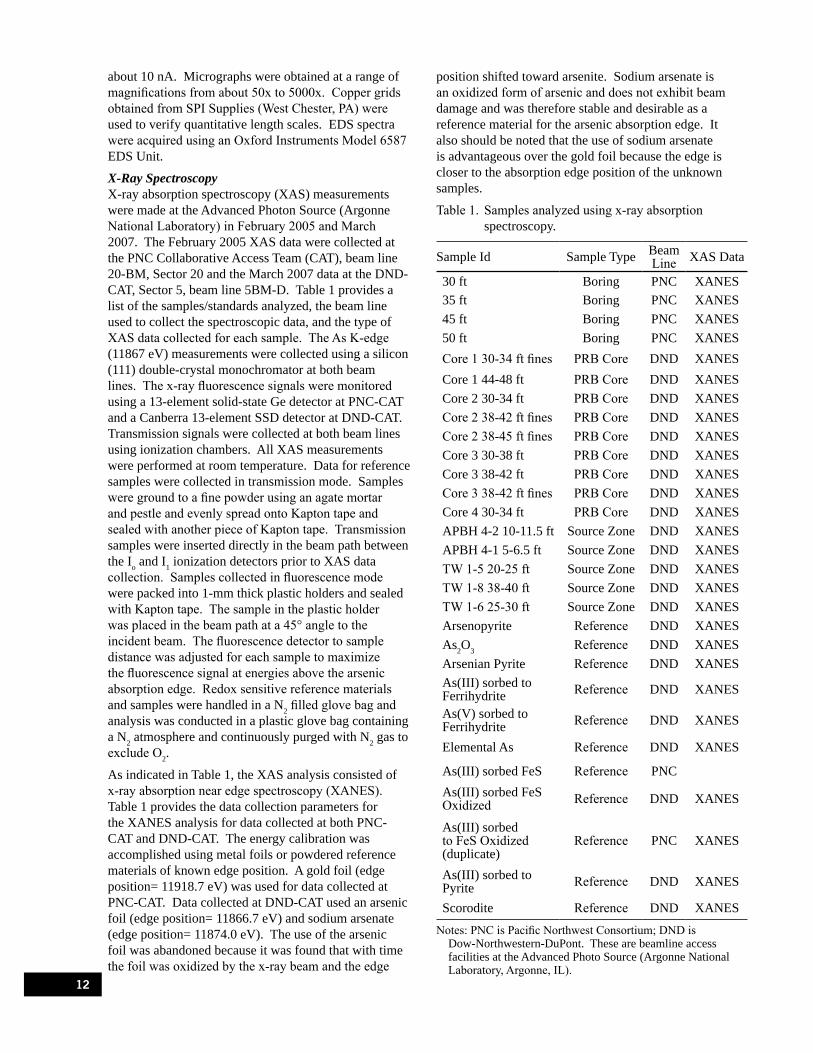
Table 1. Samples analyzed using x-ray absorption spectroscopy. . . . . . . . . . . . . . . . . . . . . . . . . . . . . . 12

Table 2. Edge and white-line positions for reference materials used in data analysis of the PRB cores, source zone materials and well borings. . . . . . . . . . . . . . . . . . . . . . . . . . . . . . . . . 13

Table 3. Comparison of hydraulic gradients calculated using multiple wells in the vicinity of the PRB and using data from three wells (DH-17, PBTW-2, and EPA08). . . . . . . . . . . . . . . . . . 14

Table 4. Ground-water parameters in selected wells. . . . . . . . . . . . . . . . . . . . . . . . . . . . . . . . . . . . . . . . 23

Table 5. Estimates of hydraulic conductivity in units of m d-1 obtained from pneumatic slug tests performed in wells located within the PRB. . . . . . . . . . . . . . . . . . . . . . . . . . . . . . . . . . . . 31

Table 6. Results of the LCF fitting of the unknown samples collected from the Asarco smelter. . . . . . 43

Table A1. Wells used in the design and assessment of the PRB. . . . . . . . . . . . . . . . . . . . . . . . . . . . . . . . 52

Table B1. Method reporting limits for selected analytes during five separate PRB sampling events and results of selected duplicate analyses. . . . . . . . . . . . . . . . . . . . . . . . . . . . . . . . . . . . . . . . 54

Table B2. Results of blank tests and pump rinsate results. . . . . . . . . . . . . . . . . . . . . . . . . . . . . . . . . . . . 55

Table C1. Thermodynamic data for arsenic oxyanions. . . . . . . . . . . . . . . . . . . . . . . . . . . . . . . . . . . . . . 56

ix

Acknowledgments

Research described in this report was partially funded by a Cooperative Research and Development Agreement (CRADA, 278-03) between ASARCO, Inc. and the U.S. EPA. The authors would like to acknowledge cooperation with ASARCO and U.S. EPA Region 8 for the successful completion of this project. Jon Nickel and Robert Miller from ASARCO are especially thanked for their helpfulness and knowledge shared during many site visits. Linda Jacobson, Randy Breeden, Chuck Figur, and Scott Brown (U.S. EPA) are thanked for their efforts in seeing this project through. Susan Zazzali (U.S. EPA) is thanked for initially focusing our attention on the East Helena site. Shaw Environmental provided support both in the field and laboratory, especially Elaine Coombe, Sujith Kumar, Don Janz, and Steve Markham. We thank Mary Sue McNeil, Pat Clark, Michael Brooks, Ken Jewell, Chunming Su, Frank Beck, Linda Callaway, Brad Scroggins, Ralph Ludwig, Robert Puls (U.S. EPA), Hsing-Lung Lien (National University of Kaohsiung, Taiwan), and Joanne Smieja (Gonzaga University) for discussions and help in the field and lab.

The authors greatly appreciate support provided by the staff of the Dow-Northwestern-DuPont Collaborative Access Team and the Pacific Northwest Consortium Collaborative Access Team at Argonne National Laboratory. Use of Argonne’s Advanced Photon Source is supported by the U. S. Department of Energy (US DOE), Office of Science, Office of Basic Energy Sciences, under Contract DE-AC02-06CH11357. PNC-XOR facilities at the Advanced Photon Source, and research at these facilities, are supported by the US DOE Basic Energy Science, a major facilities access grant from NSERC, the University of Washington, Simon Fraser University and the Advanced Photon Source. DND-CAT is supported by E.I. Dupont de Nemours & Co., the Dow Chemical Company and the State of Illinois.

The report was reviewed by Bruce Manning (San Francisco State University), Ralf Köber (University of Kiel), Kirk Scheckel (U.S. EPA), and Charles Pace (NewFields Companies LLC). Their comments helped improve the presentation and discussion of the study results.

x

Abstract

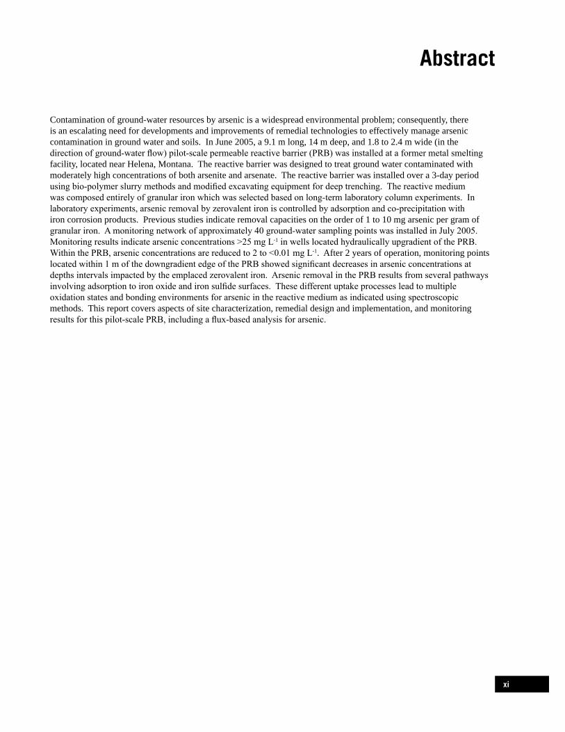
Contamination of ground-water resources by arsenic is a widespread environmental problem; consequently, there is an escalating need for developments and improvements of remedial technologies to effectively manage arsenic contamination in ground water and soils. In June 2005, a 9.1 m long, 14 m deep, and 1.8 to 2.4 m wide (in the direction of ground-water flow) pilot-scale permeable reactive barrier (PRB) was installed at a former metal smelting facility, located near Helena, Montana. The reactive barrier was designed to treat ground water contaminated with moderately high concentrations of both arsenite and arsenate. The reactive barrier was installed over a 3-day period using bio-polymer slurry methods and modified excavating equipment for deep trenching. The reactive medium was composed entirely of granular iron which was selected based on long-term laboratory column experiments. In laboratory experiments, arsenic removal by zerovalent iron is controlled by adsorption and co-precipitation with iron corrosion products. Previous studies indicate removal capacities on the order of 1 to 10 mg arsenic per gram of granular iron. A monitoring network of approximately 40 ground-water sampling points was installed in July 2005. Monitoring results indicate arsenic concentrations >25 mg L-1 in wells located hydraulically upgradient of the PRB. Within the PRB, arsenic concentrations are reduced to 2 to <0.01 mg L-1. After 2 years of operation, monitoring points located within 1 m of the downgradient edge of the PRB showed significant decreases in arsenic concentrations at depths intervals impacted by the emplaced zerovalent iron. Arsenic removal in the PRB results from several pathways involving adsorption to iron oxide and iron sulfide surfaces. These different uptake processes lead to multiple oxidation states and bonding environments for arsenic in the reactive medium as indicated using spectroscopic methods. This report covers aspects of site characterization, remedial design and implementation, and monitoring results for this pilot-scale PRB, including a flux-based analysis for arsenic.

xi

The permeable reactive barrier (PRB) technology has gained acceptance as an effective passive remediation strategy for the treatment of a variety of chlorinated organic and inorganic contaminants in ground water (e.g., O’Hannesin and Gillham, 1998; Blowes et al., 2000). The technology combines subsurface fluid-flow management with contaminant treatment by combinations of chemical, physical and/or biological processes. Application of PRBs for treatment of contaminated ground water has advantages over traditional pump-and-treat systems in that PRBs are passive and are expected to require minimal operation and maintenance expenditures. More than two hundred implementations of the technology worldwide have proven that passive reactive barriers can be cost-effective and efficient approaches to remediate a variety of hazardous compounds of environmental concern (ITRC, 2005).

Few well documented case studies are available that evaluate the field performance of these in-situ systems, especially with respect to the treatment efficiency of a variety of contaminant types and including examples from complex hydrogeologic environments. In some cases, PRB applications for ground-water remediation have failed to achieve cleanup results as expected from bench-scale tests. For example, Morrison et al. (2006) reported on a zerovalent iron system that showed

1.0 Introduction

sooner than expected breakthrough of molybdenum and uranium. Performance failure was determined to be related to a sequence of events from the continual buildup of mineral precipitates on the reactive medium, loss of pore space, development of preferential flow paths, and finally to complete bypass of the zerovalent iron and loss of hydraulic control. Research efforts over the past decade point to complex behavior in PRB systems, as biogeochemical processes in the reactive medium govern contaminant removal and influence processes that control fluid flow through porous media (e.g., U.S. EPA, 2003a; Liang et al., 2005; Li et al., 2006). Clearly these factors need to be better understood in order to improve the design and implementation of PRBs for ground-water remediation.

This report presents a pilot-scale examination of the PRB technology with zerovalent iron for treatment of arsenic in contaminated ground water. The goals of this report are to (1) document the design and construction of the pilot-scale PRB; (2) describe the hydraulic and reactive performance of the PRB; and (3) document variation in arsenic behavior and related geochemical factors within the PRB and the contaminated aquifer system. The study serves to fill in a needed aspect of the technology continuum that encompasses bench-scale testing, pilot-scale field testing, and full-scale field applications.

1

2.0 Background Arsenic in Ground Water Arsenic is a well-known toxic element that the U.S. Environmental Protection Agency and the World Health Organization list as a carcinogen. In subsurface systems, including soils, sediments, and ground water, arsenic is present in a variety of chemical forms that are influenced by changes in biogeochemical conditions. Arsenic occurs in association with minerals, such as sulfides (e.g., pyrite), metal oxides (e.g., goethite), clays, silicates, and carbonates. The most important natural sources of elevated arsenic in ground water are iron sulfides and iron oxides, partly because of the abundance of iron-containing minerals in aquifers (Smedley and Kinniburgh, 2002). Polizzoto et al. (2006) provide evidence that arsenic present in sulfide minerals is the dominant source of arsenic in Holocene aquifer sediments of Bangladesh. There arsenic released from sulfide minerals in near-surface oxidizing environments subsequently adheres to iron oxyhydroxides which are then subject to dissolution in anaerobic environments. In the anaerobic aquifer, arsenic is not retained by the aquifer solids but instead remains in the aqueous phase where tragically it is pumped through wells and consumed as drinking water by an estimated 57 million people.

As suggested above in the Bangladesh example, arsenic exhibits fairly complex chemical behavior in the environment and may be present in several oxidation states (-III, 0, III, V). In aquatic environments, two oxidation states are mainly encountered (Cherry et al., 1979; Ferguson and Gavis, 1972). The dominant form in oxic waters is arsenate, an oxyanion with the +5 oxidation state. Arsenate can be present as various protonated forms depending on pH: H3AsO4, H AsO -, HAsO 2-, and AsO 3-. In anoxic waters, the2 4 4 4 most common form of arsenic is arsenite, an uncharged species (below pH 9.2, H3AsO3) with a +3 oxidation state. Because arsenite is typically uncharged in ground-water systems, it is usually found to be mobile in solution. Ferrous iron is able to reduce arsenate to arsenite in the presence of iron oxyhydroxide surfaces, but not in homogeneous solution (Johnston and Singer, 2007a). In some ground-water settings oxygen is an available, thermodynamically favorable oxidant for arsenite. However, the rate of arsenate formation via oxidation of arsenite by molecular oxygen is generally sluggish and highly pH dependent (Cherry et al., 1979).

Toxicological studies show arsenite to be the more hazardous form of arsenic. Thus, reducing conditions, which generally favor arsenic mobility, also favor the

formation of the more toxic oxyanion of arsenic. Ground water can also contain organoarsenic species, such as monomethylarsenic acid and dimethylarsenic acid (Cullen and Reimer, 1989). In general, organoarsenic compounds are less toxic than their corresponding oxyanions. There are also arsenic-sulfur species (thioarsenic species) that provide additional complexity to arsenic speciation in reducing environments. Beak et al. (2008) indicate that at sulfide concentrations >100 µM, thioarsenic species can become dominant over the oxyanion species, arsenite and arsenate. Conversion from arsenite to thioarsenite species is believed to reduce arsenic toxicity (Rader et al., 2004). Under extremely reducing conditions elemental arsenic and arsine may be present, although their occurrence in ground water systems has not been widely documented.

Arsenate, arsenite, and thioarsenic species are highly soluble anions and will tend to remain in solution after being released from the mineral-water interface. Indeed, Magalhães (2002) points out that the primary challenge in mitigating arsenic mobility in the environment is tied to the high solubility of metal arsenites and arsenates. Under oxic conditions, arsenic can be released to ground water by dissolution of iron sulfides or by desorption from iron oxides due to an increase in pH or competition with other anions (Welch et al., 2000; Smedley and Kinniburgh, 2002). As pointed out above in the Bangladesh study, a particular geochemical environment that favors release of arsenic is the onset of iron-reducing conditions, which results from the degradation of organic carbon. Under iron-reducing conditions, arsenic associated with iron hydroxides, oxyhydroxides, or oxides can be released to ground water by reductive desorption or reductive dissolution. Reductive desorption occurs when arsenate is reduced to arsenite, which is less strongly sorbed to iron oxides; reductive dissolution of iron minerals releases arsenic that is part of the iron-mineral structure or sorbed at the mineral-water interface. On the other hand, in sulfate-reducing environments and environments where iron oxides are stable, iron sulfides and iron oxides are important sinks for arsenic, so the formation and stability of these minerals can retard the migration arsenic in ground water (U.S. EPA, 2007).

In January 2006 the U.S. Environmental Protection Agency adopted a new maximum contaminant level (MCL) for arsenic of 0.01 mg L-1, decreased from the previous level of 0.05 mg L-1. This revision of the MCL recognizes the detrimental health effects associated with arsenic in drinking water, including bladder, skin, and

2

lung cancers, diabetes, and neurological dysfunction (National Research Council, 1999). Elevated concentrations of arsenic from natural sources (>0.05 mg L-1) have been widely documented, for example, in Argentina, Bangladesh, Chile, West Bengal, Mexico, Taiwan, Mexico, and parts of the United States (e.g., Mandal, 1997; Nickson et al., 1998; Welch et al., 1988; Del Razo et al., 1990; McArthur et al., 2001; Rahman et al., 2001; Nordstrom, 2002). While arsenic occurs naturally, it may also be found as a result of a variety of industrial processes, including mining, metal refining, manufacture and use of arsenical pesticides and herbicides, release of industrial effluents, leather and wood treatments, and chemical waste disposal. These industrial activities have created a long legacy of arsenic pollution throughout the United States where arsenic is a common contaminant of concern at Superfund and RCRA sites. For example, in 1996 arsenic contamination was found at 226 Superfund sites (U.S. EPA, 1997). Levels of arsenic in ground water >1-10 mg L-1 are not unusual at many Superfund and RCRA sites in the United States. The combination of high toxicity and widespread occurrence of arsenic has created a pressing need for the development of arsenic treatment strategies in ground water. Furthermore, it is expected that the new MCL for arsenic will impact cleanup expectations at Superfund and RCRA sites across the country.

Arsenic Removal from Water by Zerovalent Iron Lackovic et al. (2000) concluded that zerovalent iron could be used in PRBs to remove inorganic forms of arsenic from ground water, including arsenate and arsenite. These researchers noted that the removal mechanism for arsenic contrasted with that of chlorinated hydrocarbons (reductive dechlorination) and hexavalent chromium (reductive precipitation), and involved either adsorption or precipitation on the iron surface. Lackovic et al. (2000) further found that arsenic removal efficiency improved with time, perhaps related to corrosion of the zerovalent iron and production of new sorption sites for arsenic uptake.

Since the Lackovic et al. (2000) study there has been a considerable research effort focused on zerovalent iron and its potential for removing arsenic from water (e.g., Ramaswami et al., 2001; Su and Puls, 2001a,b; Farrell et al., 2001; Morrison et al., 2002; Manning et al., 2002; Melitas et al., 2002; Su and Puls, 2003; Nikolaidis et al., 2003; Bang et al., 2005a,b; Lien and Wilkin, 2005; Leupin and Hug, 2005; Köber et al., 2005; Sun et al., 2006; Yuan and Chiang, 2007; Biterna et al., 2007). A common finding of these studies is that arsenic removal from water is attributable to adsorption onto corrosion products of zerovalent iron, including iron hydroxides, oxyhydroxides, and mixed valance Fe(II)-Fe(III) green rusts (Farrell et al., 2001; Melitas et al., 2002; Manning

et al., 2002; Su and Puls, 2003; Leupin and Hug, 2005; Lien and Wilkin, 2005; Bang et al., 2005b; Yuan and Chiang, 2007). Batch studies to examine the effects of anion competition for arsenite and arsenate adsorption indicate that phosphate causes a significant decrease in the removal rate of arsenic, followed by silicate, chromate, molybdate, carbonate, and nitrate (Su and Puls, 2001b). Borate and sulfate caused only slight reductions in arsenic uptake rates. Uptake capacities determined in controlled laboratory column tests have ranged from about 1 to 7.5 mg As per g of zerovalent iron (Su and Puls, 2003; Nikolaidis et al., 2003; Lien and Wilkin, 2005).

The detailed nature of arsenic uptake mechanisms onto zerovalent iron has been probed with solid-phase characterization tools sensitive to arsenic, including x-ray absorption spectroscopy, Auger electron spectroscopy, x-ray photoelectron spectroscopy, and wet chemical extractions (e.g., Su and Puls, 2001a; Farrell et al., 2001; Manning et al., 2002; Melitas et al., 2002; Nikolaidis et al., 2003; Lien and Wilkin, 2005; Bang et al., 2005a). Application of these techniques suggests that several processes may be important during the initial removal of arsenic from water and during long-term aging processes, such as adsorption, precipitation, co­precipitation, and redox transformation. For example, studies suggest that sorbed As(III) can transform to As(0) (Bang et al., 2005a) or As(V) (Su and Puls, 2001a; Manning et al., 2002; Lien and Wilkin, 2005; Leupin and Hug, 2005) depending on aging conditions, but reduction of sorbed As(V) to As(0) has not been observed (Farrell et al., 2001; Bang et al., 2005a). Reduction of As(V) to As(III) is indicated in some studies (e.g., Su and Puls, 2001a) but not in others (e.g., Farrell et al., 2001), possibly due to the variable nature of zerovalent iron and water chemistries used in laboratory experiments.

Field-based applications of zerovalent iron for arsenic treatment are few in comparison to laboratory bench tests (e.g., Morrison et al., 2002; Nikolaidis et al., 2003; Vlassopoulos et al., 2005; Bain et al., 2006), and evaluations of uptake mechanisms are not available to compare with laboratory tests. An additional factor that needs to be accounted for in field tests is the impact of microorganisms. Activity of sulfate-reducing bacteria in zerovalent iron PRBs has been documented (Roh et al., 2000; Furukawa et al., 2002; Wilkin et al., 2003, 2005). Production of biotic sulfide adds additional pathways for removal of inorganic contaminants via adsorption to and precipitation of insoluble metal sulfide precipitates. Indeed, several studies suggest that arsenic removal processes in zerovalent iron are linked to interactions with sulfur (Ramaswami et al., 2001; Nikolaidis et al., 2003; Köber et al., 2005). This pilot-scale study allows for an examination of arsenic uptake processes in a complex field setting.

3

3.0 Site Background

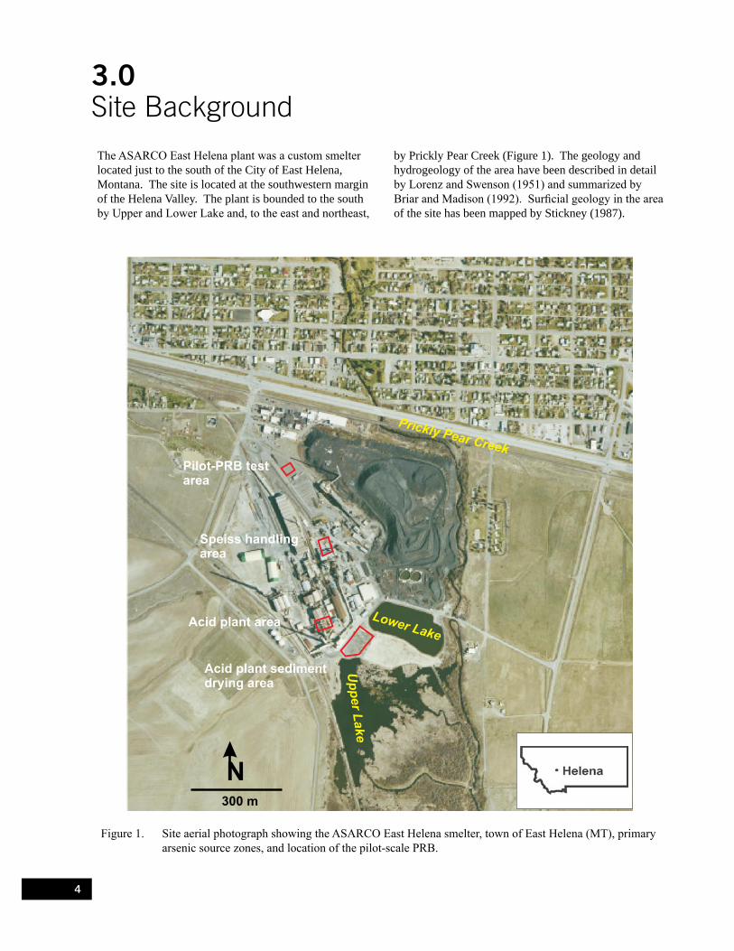
The ASARCO East Helena plant was a custom smelter located just to the south of the City of East Helena, Montana. The site is located at the southwestern margin of the Helena Valley. The plant is bounded to the south by Upper and Lower Lake and, to the east and northeast,

by Prickly Pear Creek (Figure 1). The geology and hydrogeology of the area have been described in detail by Lorenz and Swenson (1951) and summarized by Briar and Madison (1992). Surficial geology in the area of the site has been mapped by Stickney (1987).

Figure 1. Site aerial photograph showing the ASARCO East Helena smelter, town of East Helena (MT), primary arsenic source zones, and location of the pilot-scale PRB.

4

The Helena Valley is an intermontane basin bounded by sedimentary, metamorphic, and igneous rocks (Briar and Madison, 1992). The valley is underlain by a sequence of layered sediments that are not well characterized at depth. During the Quaternary period of the Cenozoic era, streams, including Prickly Pear Creek, deposited sediments in channel-fill and alluvial-plain environments over much of the central portion of the valley. The geology of the valley near the site was also affected by glaciation during the Pleistocene period. Alpine glaciers at the headwaters of Prickly Pear Creek increased the coarse sediment load of the creek through increased stream discharge during spring melting and the draining of glacial lakes. With respect to the shallow portion of the valley-fill aquifer system, these processes have resulted in a complex sequence of stratified lenses of cobbles, gravel, and sand with interlayered silt and clay. The sequence grades from predominantly cobbles, gravel, and coarse sand where streams such as Prickly Pear Creek enter the valley to predominantly sand, silt and clay near Lake Helena in the northern part of the valley.

Surface sediments at much of the plant site have been mapped by Stickney (1987) as smelter tailings. The native geologic materials bounding the northern, southern, and eastern margins of the plant are described as Holocene-age stream-channel deposits that are moderately sorted, fine to coarse sandy pebble to cobble gravel and Holocene terrace and alluvial fan deposits consisting of moderately sorted pebble to cobble gravel in a silty sandy matrix. Based on geologic logs produced from continuous split-spoon sampling at wells PBTW-1 and PBTW-2 in the area of the PRB (Figure 1), the shallow aquifer consists of relatively coarse-grained but highly variable, unconsolidated alluvial deposits containing mixtures of cobbles, gravel, sand with some silt. Fine-grained material, described as volcanic ash deposits, underlie the shallow aquifer materials in this area of the site.

The climate of the Helena Valley is semiarid with average annual precipitation between 10 and 12 inches per year in the vicinity of the site (Briar and Madison,

1992). Precipitation is generally highest during the late spring/summer months and lowest during the fall and winter months. Prickly Pear Creek, bounding the eastern portion of the smelter site and supplying water to Upper Lake at the southern site boundary, is the largest of the four principal streams flowing into the valley. During a hydrologic study performed by the U.S. Geological Survey in 1990/1991 (Briar and Madison, 1992), streamflow in Prickly Pear Creek was highest during the months of May and June and lowest during the months of December and January. The principal sources of recharge to the Helena Valley aquifer system as inferred by the 1990/1991 study are infiltration from streams, infiltration from irrigation-related sources, and inflow from fractures in surrounding bedrock.

The plant operated for over 100 years starting around 1888. Lead and zinc smelting operations resulted in the deposition of lead, arsenic, copper, zinc, cadmium, and other hazardous substances into soil and surface waters around the plant. Ground water underneath the site is contaminated in locations with arsenic, selenium, lead, cadmium, and zinc; plumes of arsenic and selenium have migrated offsite whereas the occurrence of other dissolved metals appears to be restricted within site boundaries. The East Helena Site was listed on the National Priorities List (NPL) in 1984. ASARCO shut down plant operations in April 2001 and currently plant demolitions and remedial investigations are underway.

Arsenic contamination in the ground water stems from several identified source areas. The primary source area for arsenic is located near the former speiss handling area (Figure 1). Speiss is the lightest molten phase produced in lead smelting operations and is characteristically enriched in arsenic and sometimes antimony. Other source areas include Lower Lake and the former acid plant sediment drying area. Arsenic concentrations in ground water exceed the 0.01 mg L-1 maximum concentration limit on the plant site and in an area hydraulically downgradient of the plant site. The highest concentrations occur in the former speiss handling area, the acid plant area, and the former acid plant sediment drying area.

5

4.0 PRB Installation

The pilot-PRB is a 9.1 m long (perpendicular to ground water flow), 13.7 m deep, and 1.8 to 2.4 m wide (parallel to ground water flow) installation of granular zerovalent iron (-8 + 50 mesh, Peerless Metal Powders and Abrasives, Detroit, MI). The reactive barrier was installed over a 3-day period using bio-polymer slurry methods and modified excavating equipment for deep trenching (see Figure 2 for installation photos). The reactive medium was composed entirely of granular iron which was selected based on long-term laboratory column experiments (Lien and Wilkin, 2005). The trench, located approximately 280 m hydraulically downgradient of the speiss handling area, was backfilled with a 7.6-m thick layer of granular iron (from 13.7 to 6.1 m below ground surface) and a 6.1-m thick layer of sand (from 0 to 6.1 m below ground surface). The top of the granular iron zone is located >1 m above the maximum ground water level observed during site characterization studies. The base of the granular iron zone is located approximately 1 m above the confining ash tuff deposit, and therefore the PRB is a “hanging wall”. This configuration was a planned aspect of the study in order to ensure that the lower confining unit was not breached during construction of the pilot system, to minimize costs, and to examine potential by-pass processes. The PRB contains approximately 174 t of granular iron with an initial porosity of over 50%.

After completing the backfill of granular iron and sand there was excess bio-polymer slurry in the trench and within the pore space of the zerovalent iron medium. In order to re-establish the permeability of the surrounding aquifer and to permit ground water to flow through the PRB, it was necessary to initiate breakdown of the slurry. This was accomplished by (1) breaking down the bio-polymer slurry to simple carbohydrates (monomers) and (2) encouraging native soil microbes to consume the carbohydrates. Two air lift pumps were set up to extract slurry from eight temporary wells and discharge the slurry over the surface of the backfill. The set up of the airlift pumps permitted slurry to circulate from the wells through the backfill layers and back to the wells into the reactive medium. Liquid enzyme breaker was placed into the temporary wells. The degradation or “breaking” process of the bio-polymer slurry took 3 d to complete. A Marsh funnel viscosity of less than 30 seconds indicated the slurry was broken. The pumping and slurry recirculation continued until a minimum of 3 pore volumes of the trench was circulated to flush and develop the trench.

Construction Details Shaw Environmental, Inc. performed the construction in accordance with Work Assignment WA-RB-1-8 issued by the EPA under Contract No. 68-C-03-097 (Shaw, 2005a) and described in Shaw (2005b) from which the following narrative on construction details is derived. Geo-Solutions was the subcontractor to Shaw for the bio-polymer slurry portion of the project. Prior to excavation, asphalt was cut with a walk behind saw; approximately 13 cubic yards (cy) of asphalt were disposed of offsite at the local sanitary landfill. Excavation started on June 4, 2005. The PRB trench was excavated initially with a Cat 320 smooth bucket excavator in the utility corridor. Spotters with shovels were also utilized during the first 1 m of the excavation to ensure that no underground utilities were present. A long-arm excavator (Komatsu PC750) with a ~1-m wide bucket completed the remaining trench excavation. Excavated soils were placed in a lined spoils containment area, which was located within the reach of the long-arm excavator.

Bio-polymer slurry was added to the PRB trench in order to stabilize the trench walls. Excess water in the excavated soil was allowed to spill from the excavator bucket back into the trench before unloading the soil into a lined spoils containment area. Measurement below the bio-polymer slurry level was made with a sounding cable. The slurry consisted of guar gum (Rantec G150), water, and additives. A 20,000 gallon frac tank was used to temporarily store the mixed slurry. A smaller tank was used to hold potable water prior to mixing.

Zerovalent iron was placed into the trench using tremie equipment. The tremie method was used to minimize the potential for segregation and to ensure adequate backfill density. The tremie consisted of jointed vertical pipe connected to a hopper that had legs that straddled the trench. Granular iron was backfilled into the trench from the bottom or 13.7 m below ground surface to 6.1 m below ground surface. The granular iron was delivered in “super sacks” that weighed about 3,000 pounds each. Prior to installing the PRB, the super sacks were stored at an ASARCO warehouse. The super sacks were transported to the PRB location. The granular iron was moisture conditioned and mixed with bio-polymer slurry in a bedding box prior to backfilling. The conditioned zerovalent iron was placed in the tremie hopper where it fell through a tremie pipe and flowed out on to the bottom of the trench. It was necessary to move the tremie laterally three times and raise the

6

tremie equipment vertically when the tremie pipe was filled in order to continue the backfill process. A total of 116 iron-filled super sacks was used to backfill the PRB trench.

Sand material, which consisted of coarse bedding sand, was then placed into the trench on top of the zerovalent iron. The installation work plan called for backfilling

the sand layer using the tremie system (Shaw, 2005a) to avoid segregation issues. However, the sand was backfilled using a loader bucket because segregation was not an issue with the coarse bedding sand used. The sand material was backfilled to near ground surface. Approximately 228 tons of coarse bedding sand was used.

Figure 2. Installation photos: a) long-arm excavator, b) custom bucket, c) trench with biopolymer slurry, d) excavated materials, e) bucket with aquifer materials, f) tremie and trench backfill with granular iron, g) granular iron in super sacks, and h) construction site

7

5.0 Methodology

Well Network Ground-water monitoring wells were installed in a selected region of the site for site characterization purposes prior to the installation of the pilot-PRB. Subsequently, additional monitoring wells were installed upgradient, within, and downgradient of the PRB following installation to monitor reactive and hydraulic performance of the pilot system (Figure 3). Wells within the PRB were installed using direct push methods (Geoprobe Systems). Specifically, the wells were

installed through steel rods allowing the iron to collapse around the well as the rods were removed. Most of the wells within the PRB are constructed using either 2.54 cm (1 in) or 5.08 cm (2 in) schedule 40 PVC casing and screen with a slot size of 0.051 cm (0.020 in), and are completed between 7.6 m and 14.6 m below ground surface. In addition, five wells were installed using 3.175 cm (1.25 in) OD three-channel tubing. In other wells screened across the entire saturated zone, detailed concentration and geochemical profiles were obtained

Figure 3. Aerial photos and map showing: a) arsenic concentrations in ground water (June 2006), b) locations of pilot-PRB and monitoring wells in the test area, and c) map showing well locations around and in the PRB.

8

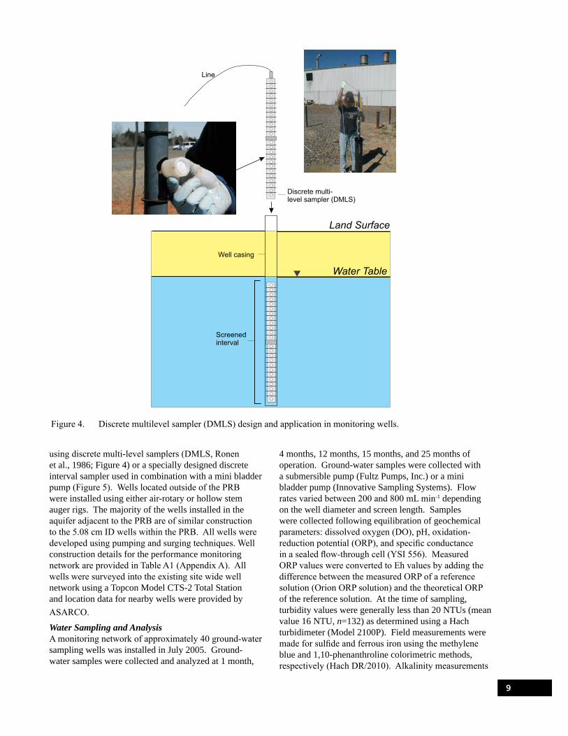
Figure 4. Discrete multilevel sampler (DMLS) design and application in monitoring wells.

using discrete multi-level samplers (DMLS, Ronen et al., 1986; Figure 4) or a specially designed discrete interval sampler used in combination with a mini bladder pump (Figure 5). Wells located outside of the PRB were installed using either air-rotary or hollow stem auger rigs. The majority of the wells installed in the aquifer adjacent to the PRB are of similar construction to the 5.08 cm ID wells within the PRB. All wells were developed using pumping and surging techniques. Well construction details for the performance monitoring network are provided in Table A1 (Appendix A). All wells were surveyed into the existing site wide well network using a Topcon Model CTS-2 Total Station and location data for nearby wells were provided by ASARCO.

Water Sampling and Analysis A monitoring network of approximately 40 ground-water sampling wells was installed in July 2005. Ground­water samples were collected and analyzed at 1 month,

4 months, 12 months, 15 months, and 25 months of operation. Ground-water samples were collected with a submersible pump (Fultz Pumps, Inc.) or a mini bladder pump (Innovative Sampling Systems). Flow rates varied between 200 and 800 mL min-1 depending on the well diameter and screen length. Samples were collected following equilibration of geochemical parameters: dissolved oxygen (DO), pH, oxidation-reduction potential (ORP), and specific conductance in a sealed flow-through cell (YSI 556). Measured ORP values were converted to Eh values by adding the difference between the measured ORP of a reference solution (Orion ORP solution) and the theoretical ORP of the reference solution. At the time of sampling, turbidity values were generally less than 20 NTUs (mean value 16 NTU, n=132) as determined using a Hach turbidimeter (Model 2100P). Field measurements were made for sulfide and ferrous iron using the methylene blue and 1,10-phenanthroline colorimetric methods, respectively (Hach DR/2010). Alkalinity measurements

9

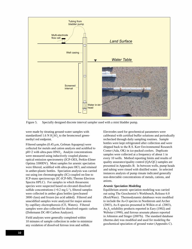
Figure 5. Specially designed discrete interval sampler used with a mini bladder pump.

were made by titrating ground-water samples with standardized 1.6 N H2SO4 to the bromcresol green-methyl red endpoint.

Filtered samples (0.45 µm, Gelman Aquaprep) were collected for metals and cation analysis and acidified to pH<2 with ultra-pure HNO3. Analyte concentrations were measured using inductively coupled plasma – optical emission spectrometry (ICP-OES, Perkin-Elmer Optima 3300DV). Most samples for arsenic speciation were filtered, acidified with ultra-pure HCl, and retained in amber-plastic bottles. Speciation analysis was carried out using ion chromatography (IC) coupled on-line to ICP-mass spectroscopy (IC-ICP-MS; Thermo Electron Spectra HPLC). For samples in which thioarsenic species were suspected based on elevated dissolved sulfide concentrations (>0.2 mg L-1), filtered samples were collected in amber glass bottles (precleaned 3000 class) and frozen (no acid added). Filtered and unacidified samples were analyzed for major anions by capillary electrophoresis (CE, Waters). Filtered samples were also collected for dissolved organic carbon (Dohrmann DC-80 Carbon Analyzer).

Field analyses were generally completed within 10 minutes of sample collection in order to minimize any oxidation of dissolved ferrous iron and sulfide.

Electrodes used for geochemical parameters were calibrated with certified buffer solutions and periodically rechecked through daily sampling routines. Sample bottles were kept refrigerated after collection and were shipped back to the R.S. Kerr Environmental Research Center (Ada, OK) in ice-packed coolers. Duplicate samples were collected at a frequency of about 1 in every 10 wells. Method reporting limits and results of quality assurance/quality control (QA/QC) samples are presented in Appendix B. In between wells, pump heads and tubing were rinsed with distilled water. In selected instances analysis of pump rinsate indicated generally non-detectable concentrations of metals, cations, and anions.

Arsenic Speciation Modeling Equilibrium arsenic speciation modeling was carried out using The Geochemist’s Workbench, Release 6.0 (RockWare). Thermodynamic databases were modified to include the As-O species in Nordstrom and Archer (2003), As-S species presented in Wilkin et al. (2003), As2S3 solubility products reported in Eary (1992) and Webster (1990), and ferrous arsenate phases reported in Johnston and Singer (2007b). The standard database (thermo.dat) was modified and used for modeling the geochemical speciation of ground water (Appendix C).

10

Core Sampling and Analysis Core samples from the PRB were collected after 15 months to assess the uptake of arsenic and to evaluate corrosion and mineral buildup on the iron surfaces. Core collection methods and analysis procedures are described in previous publications on PRB long-term performance (U.S. EPA, 2003a,b). In all cases 5 cm inner diameter cores were collected using a Geoprobe™. Core barrels were driven using a pneumatic hammer to the desired sampling location and continuous, up to 110 cm, sections of iron or iron + soil were retrieved. Vertical cores were collected in order to determine the spatial distribution of mineral buildup in the reactive medium. Angle cores were not collected; direct push methods were incapable of advancing core barrels through the subsurface but were amenable in the gravelly fill directly above the iron and in the PRB. Core materials from the East Helena PRB were black to gray in color without any obvious signs of cementation or oxidation (Figure 6).

Figure 6. Photograph of a core segment collected from the PRB after 15 months of operation (September 2006).

Immediately after collection, the cores were frozen and shipped back to the R.S. Kerr Environmental Research Center for sub-sampling and analysis. The frozen cores were partially thawed and then placed in an anaerobic chamber with a maintained H2-N2 atmosphere. Each core was logged and partitioned into 5 to 10 cm

segments. Each segment was homogenized by stirring in the glove box and then split into 3 sub-samples for: (1) inorganic carbon analyses, (2) sulfur analyses/x-ray diffraction (XRD)/x-ray absorption spectroscopy, and (3) Scanning electron microscopy (SEM). All sub-samples were retained in airtight vials to prevent any air oxidation of redox-sensitive constituents.

To determine elemental concentrations in bulk solids, samples were digested in a microwave oven in 10% nitric acid, and digestates were analyzed for metals and non-metals by the same methods as those used for ground water analysis. Concentrations of inorganic carbon in core samples were determined with a carbon coulometer system (UIC, Inc. Model CM5014). Inorganic carbon analysis results are given in weight percent C based upon carbon released from a sample after acidification with hot 5% perchloric acid. This acid digestion procedure releases inorganic carbon present in minerals such as calcite (trigonal CaCO3), aragonite (orthorhombic CaCO3), siderite (FeCO3), magnesite (MgCO3), rhodochrosite (MnCO3), ferrous carbonate hydroxide (Fe2(OH)2CO3), and carbonate green rust (Fe6(OH)12CO3·2H2O). Measurements of totalsulfur in the solid phase were carried out using a sulfur coulometer (UIC, Inc. Model CM5014S) in combustion mode. Details of the sulfur measurement method are described in Wilkin and Bischoff (2006).

Powder x-ray diffraction analysis of core samples collected from the East Helena site was conducted to determine the mineralogy of the aquifer materials and precipitates formed in the iron treatment zones. Materials for analysis were prepared by sonicating iron core samples in acetone for 10 minutes followed by filtration of the released particulates through 47 mm diameter, 0.2-µm filter paper (polycarbonate). The separated particles were mounted on a zero-background quartz plate and scanned with Fe Kα radiation from 10° to 90° 2-theta using a Rigaku Miniflex Diffractometer. Scanning electron microscopy (SEM) and energy dispersive x-ray spectroscopy (EDS) was used to evaluate the morphology and composition of mineral precipitates on the surfaces of zero-valent iron particles collected at the East Helena site. Measurements were conducted on polished samples to determine the composition of surface precipitates on a semi-quantitative basis. Samples for SEM and EDS analyses were stored in an anaerobic glove box and then embedded in an epoxy resin. The sample mounts (2.5 cm diameter round mounts) were ground and polished using diamond abrasives and coated with a thin layer of gold prior to being placed within the SEM sample chamber. Secondary electron and back-scattered electron images were obtained using a JEOL JSM-6360 SEM. The instrument was operated using a 20 kV electron accelerating potential and a beam current of

11

about 10 nA. Micrographs were obtained at a range of magnifications from about 50x to 5000x. Copper grids obtained from SPI Supplies (West Chester, PA) were used to verify quantitative length scales. EDS spectra were acquired using an Oxford Instruments Model 6587 EDS Unit.

X-Ray Spectroscopy X-ray absorption spectroscopy (XAS) measurements were made at the Advanced Photon Source (Argonne National Laboratory) in February 2005 and March 2007. The February 2005 XAS data were collected at the PNC Collaborative Access Team (CAT), beam line 20-BM, Sector 20 and the March 2007 data at the DND­CAT, Sector 5, beam line 5BM-D. Table 1 provides a list of the samples/standards analyzed, the beam line used to collect the spectroscopic data, and the type of XAS data collected for each sample. The As K-edge (11867 eV) measurements were collected using a silicon (111) double-crystal monochromator at both beam lines. The x-ray fluorescence signals were monitored using a 13-element solid-state Ge detector at PNC-CAT and a Canberra 13-element SSD detector at DND-CAT. Transmission signals were collected at both beam lines using ionization chambers. All XAS measurements were performed at room temperature. Data for reference samples were collected in transmission mode. Samples were ground to a fine powder using an agate mortar and pestle and evenly spread onto Kapton tape and sealed with another piece of Kapton tape. Transmission samples were inserted directly in the beam path between the Io and I1 ionization detectors prior to XAS data collection. Samples collected in fluorescence mode were packed into 1-mm thick plastic holders and sealed with Kapton tape. The sample in the plastic holder was placed in the beam path at a 45° angle to the incident beam. The fluorescence detector to sample distance was adjusted for each sample to maximize the fluorescence signal at energies above the arsenic absorption edge. Redox sensitive reference materials and samples were handled in a N2 filled glove bag and analysis was conducted in a plastic glove bag containing a N2 atmosphere and continuously purged with N2 gas to exclude O2.

As indicated in Table 1, the XAS analysis consisted of x-ray absorption near edge spectroscopy (XANES). Table 1 provides the data collection parameters for the XANES analysis for data collected at both PNC­CAT and DND-CAT. The energy calibration was accomplished using metal foils or powdered reference materials of known edge position. A gold foil (edge position= 11918.7 eV) was used for data collected at PNC-CAT. Data collected at DND-CAT used an arsenic foil (edge position= 11866.7 eV) and sodium arsenate (edge position= 11874.0 eV). The use of the arsenic foil was abandoned because it was found that with time the foil was oxidized by the x-ray beam and the edge

position shifted toward arsenite. Sodium arsenate is an oxidized form of arsenic and does not exhibit beam damage and was therefore stable and desirable as a reference material for the arsenic absorption edge. It also should be noted that the use of sodium arsenate is advantageous over the gold foil because the edge is closer to the absorption edge position of the unknown samples.

Table 1. Samples analyzed using x-ray absorption spectroscopy.

Sample Id Sample Type Beam Line XAS Data

30 ft Boring PNC XANES 35 ft Boring PNC XANES 45 ft Boring PNC XANES 50 ft Boring PNC XANES Core 1 30-34 ft fines PRB Core DND XANES Core 1 44-48 ft PRB Core DND XANES Core 2 30-34 ft PRB Core DND XANES Core 2 38-42 ft fines PRB Core DND XANES Core 2 38-45 ft fines PRB Core DND XANES Core 3 30-38 ft PRB Core DND XANES Core 3 38-42 ft PRB Core DND XANES Core 3 38-42 ft fines PRB Core DND XANES Core 4 30-34 ft PRB Core DND XANES APBH 4-2 10-11.5 ft Source Zone DND XANES APBH 4-1 5-6.5 ft Source Zone DND XANES TW 1-5 20-25 ft Source Zone DND XANES TW 1-8 38-40 ft Source Zone DND XANES TW 1-6 25-30 ft Source Zone DND XANES Arsenopyrite Reference DND XANES As2O3 Reference DND XANES Arsenian Pyrite Reference DND XANES As(III) sorbed toFerrihydrite Reference DND XANES

As(V) sorbed toFerrihydrite Reference DND XANES

Elemental As Reference DND XANES

As(III) sorbed FeS Reference PNC As(III) sorbed FeSOxidized Reference DND XANES

As(III) sorbedto FeS Oxidized Reference PNC XANES (duplicate) As(III) sorbed toPyrite Reference DND XANES

Scorodite Reference DND XANES Notes: PNC is Pacific Northwest Consortium; DND is

Dow-Northwestern-DuPont. These are beamline access facilities at the Advanced Photo Source (Argonne National Laboratory, Argonne, IL).

12

Raw XANES data were processed using the Athena software package (Ravel and Newville, 2005) that is based on the IFEFFIT procedures (Newville, 2001). Multiple scans (2 to 10 scans depending on data quality and depending on whether the scans were collected in fluorescence or transmission mode) of each sample were collected and each scan was aligned using a reference spectrum shown in Table 1. The aligned spectra were merged into a final spectrum for each sample. The merged averaged spectra were background corrected and step height normalized. The normalized data were used for XANES and linear combination of fits (LCF) analysis. XANES and LCF operations were processed using Athena. XANES analysis consisted of examining the first derivative of the spectrum to determine the edge position and comparing the edge position to standard reference materials. The edge position of the standard reference materials was used to help determine the local bonding environment surrounding the arsenic atom (see Table 2). Similarly, the white line position could be determined using the raw spectrum and the white line position could also be used to determine the local bonding environment around the central arsenic atom (Table 2).

Table 2. Absorption edge and white-line positions of reference materials used in data analysis of the PRB cores, source zone materials and well borings.

Compound Edge Position (eV)

White Line (eV)

Elemental As

Orpiment

As(III) sorbed FeS

11866.7

11868.7

11867.6

11868.7

11870.1

11870.5

As(III) sorbed to Ferrihydrite

Sodium Arsenite

11869.9

11870.1

11871.9

11871.8

Enargite

Sodium Arsenate

As(V) sorbed to Ferrihydrite

11870.2

11874.0

11873.8

11871.7

11875.5

11875.5

Scorodite 11874.0 11875.8

Notes: Edge position is defined as the maximum in the first-derivative of the energy vs. absorption function. White line position is defined as the maximum in the energy vs. absorption function.

LCF analysis was accomplished using the Athena software package. The LCF analysis was used to determine the types of bonding environments in the samples. In addition, LCF can be used to give the relative contribution of each bond type in the analyzed samples. The LCF fitting was accomplished using the normalized XANES over the fit range: -20 eV < E0 < 30 eV . The data were fitted using all possible combinations of standards and the fit weights were forced to be ≥ 0. Initially LCF analysis was used to determine the types of arsenic bonds present (e.g., As-S, As-O) as well as the formal oxidation state of arsenic. This type of fitting was accomplished using mineral phases of known valence and bond type: elemental arsenic (As(0)), sodium arsenite (As(III)-O), sodium arsenate (As(V)-O), orpiment (As(III)-S), enargite (4:1 As(V)-S), and dimethyl thioarsenate (2:1 As(V)-S, DMTA). In all samples it was found that only As(V)-O, As(III)-O, and As(III)-S had contributing fractions above 0. Additional LCF analysis was carried out on the samples using As(III) or As(V) sorbed to specific iron mineral phases. The significant phases were likely As(III) sorbed to ferrihydrite, As(V) sorbed to ferrihydrite, and As(III) sorbed to FeS.

Hydrologic Methods Hydraulic gradients at the water table were estimated using both potentiometric surfaces interpreted from manual ground-water elevation measurements and from solution of the three-point problem using data from wells instrumented with pressure transducers/data loggers. A method similar to that described in Devlin (2003) was used for automated solution of the three-point problem. Gradients were estimated by fitting a plane to the hydraulic head data using multiple linear regression techniques. The hydraulic gradients calculated using the three-point solution were compared with estimates of gradients from potentiometric surfaces and found to be similar (Table 3). This allowed gradients to be estimated on a daily basis and averages more representative of the full range of hydrologic conditions to be calculated.

13

Table 3. Comparison of hydraulic gradients calculated using multiple wells in the vicinity of the PRB and using data from three wells (DH-17, PBTW-2, and EPA08).

Measurement Date

Multi-Point Estimate Three-Point Estimate Direction DirectionMagnitude Magnitude(degrees) (degrees)

10/6/05 0.005 336 0.005 335

6/6/06 0.008 342 0.008 323

9/18/06 0.005 338 0.005 339

7/19/07 0.005 331 0.005 345

10/1/07 0.005 335 0.005 335

4/1/08 0.006 329 0.006 331

Field measurements of hydraulic conductivity were made using single-well pumping tests and pneumatic slug testing. Pneumatic slug tests within the PRB have been performed using equipment similar to that depicted in Figure 7. This method is based on recommendations derived from Butler (1997) and utilizes air pressure and vacuum to initiate instantaneous changes in head within the well combined with high frequency monitoring of the aquifer response using data loggers and pressure transducers. This type of test provides the instantaneous change in hydraulic head needed for the performance of meaningful slug tests in media with high hydraulic conductivity. The response data were analyzed using the methods of Bouwer and Rice (1976), Springer and Gelhar (1991), and Butler and Garnett (2000).

A sensitive electromagnetic borehole flowmeter was used to define the relative hydraulic conductivity

14

Figure 7. Typical equipment used in performance of pneumatic slug tests.

distribution of aquifer materials within and in the vicinity of the pilot-PRB. The studies consisted of measuring the vertical component of ground water flow at fixed intervals in the wells under undisturbed (ambient) and pumping conditions (Figure 8). Measurements were made during constant-rate ground water extraction to define the distribution of ground water flow to the well. The rate of water flow to the well from an individual interval is proportional to the hydraulic conductivity of the materials adjacent to the screen. Therefore, knowledge of the contribution of flow from each measurement interval allows interpretation of the hydraulic conductivity structure relative to the average hydraulic conductivity of materials screened by the well (Molz et al., 1994; Young et al., 1998).

Figure 8. Schematic diagram of electromagnetic borehole flowmeter test design.

The electromagnetic borehole flowmeter used in these studies was a commercially available system manufactured by Tisco, Inc., consisting of a 1.3-cm ID downhole probe, a 2.5-cm ID downhole probe, and an electronics module. Probe design is based on Faraday’s Law which states that the voltage induced by an electrical conductor moving through a magnetic field is directly proportional to the velocity of the conductor. The major components of the probe include an electromagnet and a pair of electrodes mounted at right

angles to the poles of the magnet. The downhole probe is designed as a hollow iron core through which water flows. The electromagnet surrounding the core produces a strong magnetic field. A voltage that is proportional to the average water velocity is generated as the conductor (i.e., ground water) flows through the magnetic field. An uphole electronics package connected to the probe amplifies and displays the voltage signal. Real-time data acquisition is controlled by an associated computer. The system is capable of measuring flow rates ranging from less than 0.040 L min-1 to 40 L min-1.

Prior to conducting the study, the flowmeter was calibrated in test cells constructed of materials identical to those of well construction. Calibration was performed by measuring water discharge from the test cell using graduated cylinders and comparison with the associated voltage measured by the flowmeter. Flow rates were chosen to span the range of rates that would be used in the field. Data obtained during the calibration phase indicated that the meter responses for both the 1.3-cm ID probe and the 2.5-cm ID probe were linear over the range of potentially applicable flow rates.

The field tests were conducted using a procedure based on the methods of Molz et al. (1994) and Young et al. (1998). Flow rate measurements using the electromagnetic borehole flowmeter were made under ambient and constant-rate pumping conditions at a measurement interval between 30 cm and 60 cm within the well screen. The use of the 1.3-cm ID probe was attempted for flow measurements under ambient conditions. However, extreme variability, which was likely due to electromagnetic interference from outside sources, necessitated the use of the less sensitive, 2.5-cm ID probe which was used for all measurements under pumping conditions. The tests were performed at constant pumping rates ranging from 3 L min-1 to 7 L min-1. The rates were chosen to induce sufficient flow from each test interval with negligible head loss across the downhole probe. Each test was performed using the following general protocol:

1. Ambient vertical flow rates were measured from total depth to the top of the screen or water table under static conditions.

2. The 2.5-cm ID probe was lowered to the bottom of the well. A submersible pump was installed at the water table and pumping was initiated to establish a horizontal flow field. A pressure transducer and data logger were used to monitor the water-level response to groundwater extraction. The discharge rate from the pump was measured using a graduated cylinder and a stop watch at intervals not exceeding approximately 30 min.

3. The establishment of a steady horizontal flow field was indicated by stability in the pressure response to

15

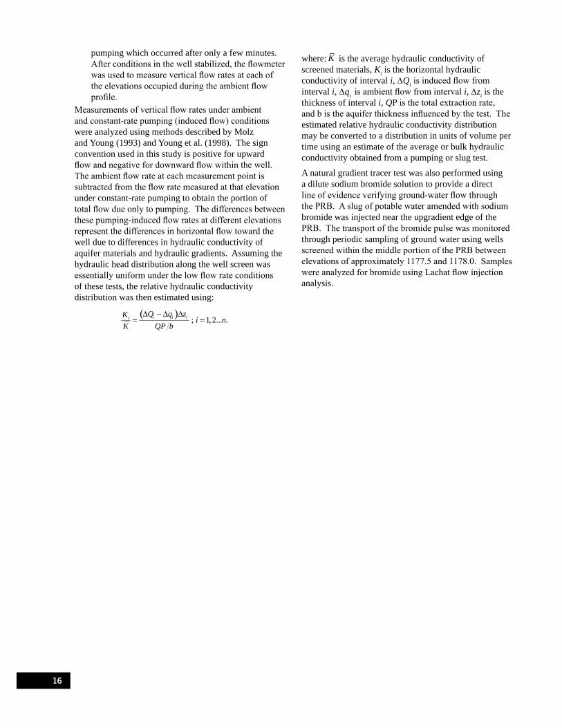
K (∆Q − ∆ q )∆zi i i i= ; i = 1, 2... n.K QP b

pumping which occurred after only a few minutes. After conditions in the well stabilized, the flowmeter was used to measure vertical flow rates at each of the elevations occupied during the ambient flow profile.

Measurements of vertical flow rates under ambient and constant-rate pumping (induced flow) conditions were analyzed using methods described by Molz and Young (1993) and Young et al. (1998). The sign convention used in this study is positive for upward flow and negative for downward flow within the well. The ambient flow rate at each measurement point is subtracted from the flow rate measured at that elevation under constant-rate pumping to obtain the portion of total flow due only to pumping. The differences between these pumping-induced flow rates at different elevations represent the differences in horizontal flow toward the well due to differences in hydraulic conductivity of aquifer materials and hydraulic gradients. Assuming the hydraulic head distribution along the well screen was essentially uniform under the low flow rate conditions of these tests, the relative hydraulic conductivity distribution was then estimated using:

where: K is the average hydraulic conductivity of screened materials, Ki is the horizontal hydraulic conductivity of interval i, ∆Qi is induced flow from interval i, ∆qi is ambient flow from interval i, ∆zi is the thickness of interval i, QP is the total extraction rate, and b is the aquifer thickness influenced by the test. The estimated relative hydraulic conductivity distribution may be converted to a distribution in units of volume per time using an estimate of the average or bulk hydraulic conductivity obtained from a pumping or slug test.

A natural gradient tracer test was also performed using a dilute sodium bromide solution to provide a direct line of evidence verifying ground-water flow through the PRB. A slug of potable water amended with sodium bromide was injected near the upgradient edge of the PRB. The transport of the bromide pulse was monitored through periodic sampling of ground water using wells screened within the middle portion of the PRB between elevations of approximately 1177.5 and 1178.0. Samples were analyzed for bromide using Lachat flow injection analysis.

16

Ground-water Geochemistry A snapshot trend of major ion chemistry across the site, from the primary source area for arsenic downgradient to the PRB location and further to the site boundary, is shown using a modified Durov diagram (Figure 9). Ground water in the former speiss handling area is slightly alkaline (pH ~10), and elevated in total dissolved solids (TDS>3500 mg L-1) and arsenic (>100 mg L-1). Sodium is the major cation and approximately equimolar concentrations of bicarbonate and sulfate are present in ground water near the source area for arsenic. Downgradient from the former speiss handling area, ground water evolves to lower pH (~6.5), TDS values (<1500 mg L-1), and arsenic concentrations (<50 mg L-1); sulfate becomes the dominant anion and the proportion increases of calcium and magnesium relative to sodium (Figure 9).

6.0 Results and Discussion

Long-term trends in the major ion chemistry of ground water near the PRB test area are shown in a series of Stiff diagrams on Figure 10 constructed using data from well PBTW-1 (see Figure 3). These plots show little variation over about six years in the proportions and absolute concentrations of major cations and anions sampled from monitoring well PBTW-1. In the area of the pilot-PRB and over most of the site, ground water is generally of Na+-SO4

2- type, with Na+ (150-900 mg L-1) and SO4

2- (300-1000 mg L-1). On a molar basis, sodium is enriched over calcium by about 6 times and sulfate is enriched over bicarbonate by about 3 times. Variations in ground water chemistry can be attributed to interactions between ground water, aquifer minerals, and wastes generated on the plant site.

Geochemical profiles across the entire saturated zone for selected wells are shown on Figure 11. These depth

Figure 9. Modified Durov diagram showing trends in major cations, anions, total dissolved solids, and arsenic concentrations from the former speiss handling area to the northern site boundary (data collected June 2006).

17

profiles were obtained using a multi-layer sampler with baffles fit flush to the well casing, enabling sampling of discrete depth intervals in the saturated zone (Ronen et al., 1986). At well locations PBTW-1 and PBTW-2, solute profiles are relatively uniform with no sharp concentration gradients. Concentrations of total arsenic vary between about 40 and 50 mg L-1 across the entire saturated thickness in these wells. Arsenic speciation results indicate that arsenite is the dominant form of arsenic with some As(V) detected (2 to 14% of the total arsenic, excluding the shallowest sampling point in well PBTW-1). Wells DH-50 and EPA04 show more pronounced chemical gradients (Figure 11c,d). For example, a 3-fold increase in arsenic concentration is observed at the base of well DH-50, which corresponds with a change in aquifer geology from a sandy matrix to a sandy matrix mixed with coarse gravel and cobbles. In well EPA04, located near the pilot-scale PRB (Figure 11c), a transition in arsenic concentration is observed at a depth of about 12 m below ground surface, a concentration trend mirrored by sulfate and specific conductance. Monitoring well results are also shown on Figure 11 for samples collected at comparable

times for which the discrete interval sampling was carried out. In most cases, the bulk well results give a good representation of the average chemistry across the saturated aquifer.

Arsenic concentrations in ground-water samples collected over a period of 6 y vary from below detection limits to a high value of 238 mg L-1. A comparison between total dissolved arsenic concentrations and the sum of arsenic species (arsenite + arsenate) is shown on Figure 12. In over 90% of the samples, total arsenic values are in very good agreement with the sum of arsenic species (±10%). There appears to be a tendency for the sum of arsenite plus arsenate to be slightly less than the measured total arsenic value. This slight discrepancy is likely related to a bias stemming from the large dilutions often necessary to conduct the speciation analysis on high concentration samples rather than to the possibility of there being a missing species of arsenic unaccounted for in the speciation analysis. As will be discussed later, thioarsenic species are present in some wells located within the PRB. Organic species of arsenic were not detected during this study.

18

Figure 10. Long-term trends in the major ion chemistry of ground water collected from monitoring well PBTW-1.

Figure 11. Geochemical profiles across the saturated aquifer in selected wells: a) PBTW-1, b) PBTW-2, c) EPA04, and d) DH-50 (see Figure 3 for well locations).

19

Figure 11. Geochemical profiles across the saturated aquifer in selected wells: a) PBTW-1, b) PBTW-2, c) EPA04, and d) DH-50 (see Figure 3 for well locations).

20

Figure 12. Comparison of total dissolved arsenic concentrations and the sum of arsenate plus arsenite.

Figure 13 shows a comparison between arsenic concentrations in ground water and the pH-dependent solubility of As2O3 and As2O5. This figure illustrates that site ground water, even with high levels of arsenic present, is still highly undersaturated with respect to possible solubility controlling phases, As2O3 and As2O5. In a following section this analysis is extended to examine other possible phases that form in and around the PRB, yet the trends indicate that factors controlling arsenic concentrations in ground water are primarily controlled by mineral-water reactions taking place in the source area and dilution during transport, rather than to retardation and arsenic attenuation by aquifer solids. Redox conditions also impact the mobility and observed arsenic concentration distributions. The highest total arsenic concentrations are typically observed when arsenic is dominated by arsenite (Figure 14); thus, reducing conditions presumably play a role in governing the plume dynamics. This correlation between reducing conditions and elevated arsenic concentrations is also shown on Figure 15 where ferrous iron concentrations and Eh in ground water are contoured in the area around the PRB. Note that ferrous iron and Eh values <150 mV are typical in areas where arsenic concentrations are high. Where ferrous iron concentrations are low (<0.5 mg L-1), arsenic is generally present at lower concentrations (<10 mg L-1) as arsenate.

Figure 13. Arsenic concentrations in solutions saturated with As2O5 and As2O3 and site ground water (open red circles) compared to the MCL for arsenic.

Figure 14. Comparison of total dissolved arsenic and the fraction of total dissolved arsenic present as arsenite, As(III).

21

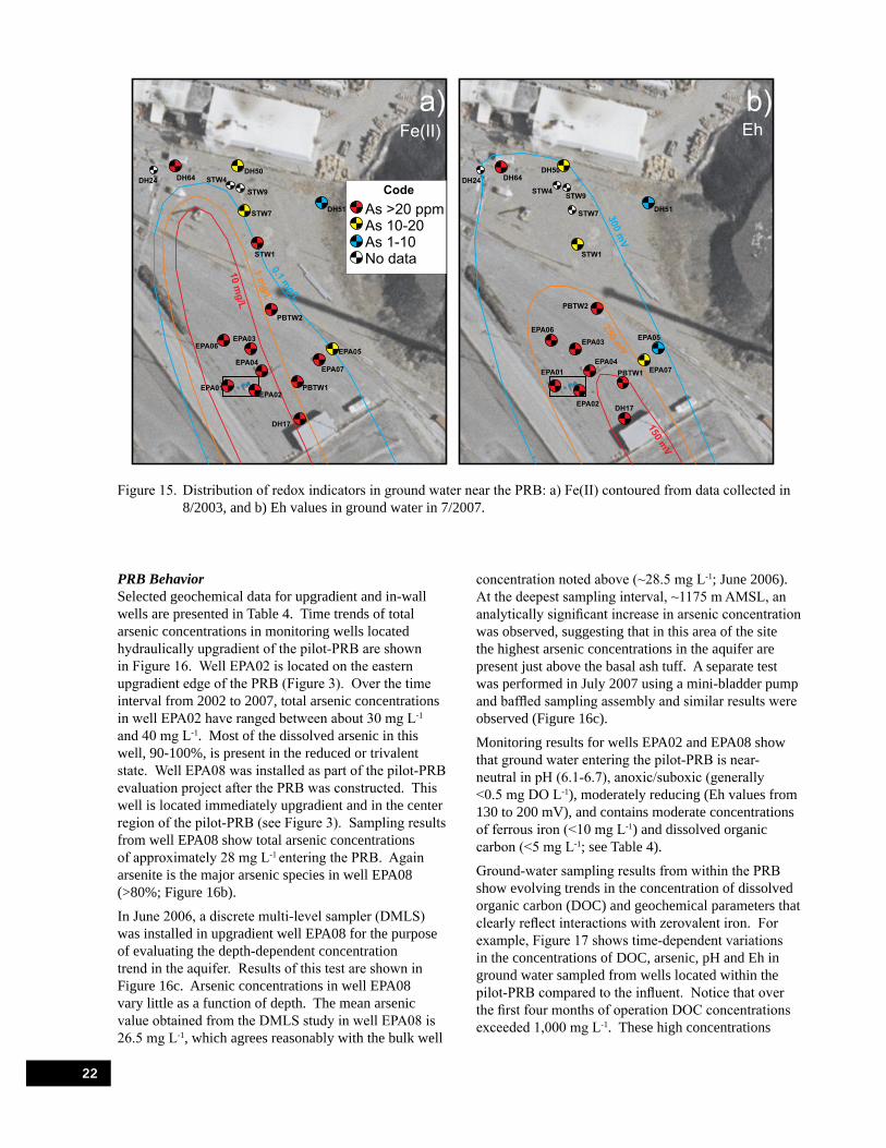
Figure 15. Distribution of redox indicators in ground water near the PRB: a) Fe(II) contoured from data collected in 8/2003, and b) Eh values in ground water in 7/2007.

PRB Behavior Selected geochemical data for upgradient and in-wall wells are presented in Table 4. Time trends of total arsenic concentrations in monitoring wells located hydraulically upgradient of the pilot-PRB are shown in Figure 16. Well EPA02 is located on the eastern upgradient edge of the PRB (Figure 3). Over the time interval from 2002 to 2007, total arsenic concentrations in well EPA02 have ranged between about 30 mg L-1

and 40 mg L-1. Most of the dissolved arsenic in this well, 90-100%, is present in the reduced or trivalent state. Well EPA08 was installed as part of the pilot-PRB evaluation project after the PRB was constructed. This well is located immediately upgradient and in the center region of the pilot-PRB (see Figure 3). Sampling results from well EPA08 show total arsenic concentrations of approximately 28 mg L-1 entering the PRB. Again arsenite is the major arsenic species in well EPA08 (>80%; Figure 16b).

In June 2006, a discrete multi-level sampler (DMLS) was installed in upgradient well EPA08 for the purpose of evaluating the depth-dependent concentration trend in the aquifer. Results of this test are shown in Figure 16c. Arsenic concentrations in well EPA08 vary little as a function of depth. The mean arsenic value obtained from the DMLS study in well EPA08 is 26.5 mg L-1, which agrees reasonably with the bulk well

concentration noted above (~28.5 mg L-1; June 2006). At the deepest sampling interval, ~1175 m AMSL, an analytically significant increase in arsenic concentration was observed, suggesting that in this area of the site the highest arsenic concentrations in the aquifer are present just above the basal ash tuff. A separate test was performed in July 2007 using a mini-bladder pump and baffled sampling assembly and similar results were observed (Figure 16c).

Monitoring results for wells EPA02 and EPA08 show that ground water entering the pilot-PRB is near-neutral in pH (6.1-6.7), anoxic/suboxic (generally <0.5 mg DO L-1), moderately reducing (Eh values from 130 to 200 mV), and contains moderate concentrations of ferrous iron (<10 mg L-1) and dissolved organic carbon (<5 mg L-1; see Table 4).

Ground-water sampling results from within the PRB show evolving trends in the concentration of dissolved organic carbon (DOC) and geochemical parameters that clearly reflect interactions with zerovalent iron. For example, Figure 17 shows time-dependent variations in the concentrations of DOC, arsenic, pH and Eh in ground water sampled from wells located within the pilot-PRB compared to the influent. Notice that over the first four months of operation DOC concentrations exceeded 1,000 mg L-1. These high concentrations

22

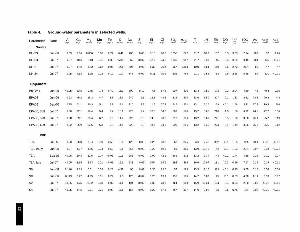
Table 4. Ground-water parameters in selected wells.

Parameter Date Al(mg/L)

Ca(mg/L)

Mg(mg/L)

Mn(mg/L)

Fe(mg/L)

K(mg/L)

Na(mg/L)

Zn(mg/L)

Si(mg/L)

Cl(mg/L)

SO4(mg/L)

HCO3(mg/L)

T(°C)

pH(SU)

Eh(mV)

DO(mg/L)

SC(mS/cm)

TOC(mg/L)

As(mg/L)

As(III)(mg/L)

As(V)(mg/L)

Source

DH-33 Jun-06 0.09 2.96 0.836 0.10 0.27 6.41 786 0.06 3.10 60.0 1050 672 11.7 10.2 157 0.3 3.03 7.14 103 87 1.26

DH-33 Jul-07 0.07 10.6 8.43 0.31 0.36 5.85 869 <0.02 3.17 74.8 1050 917 11.7 9.39 15 0.5 3.29 9.45 104 105 <0.01

DH-21 Jul-07 0.07 14.2 6.82 0.62 0.06 14.5 807 0.03 6.30 25.4 557 1383 10.9 8.81 189 3.6 2.73 21.4 89 47 47

DH-34 Jul-07 0.05 4.13 1.78 0.02 0.12 19.0 548 <0.02 6.11 30.2 502 786 11.1 9.58 68 0.6 2.38 5.88 99 101 <0.01

Upgradient

PBTW-1 Jun-06 <0.05 32.5 9.45 1.4 0.40 11.9 509 0.10 7.8 67.3 907 420 13.4 7.50 173 0.2 2.04 4.50 45 40.4 0.95

EPA08 Jun-06 0.23 45.2 18.3 4.7 5.5 13.9 249 2.1 13.5 42.5 514 300 13.6 6.50 207 0.1 1.33 3.62 28.5 20.2 4.8

EPA08 Sep-06 0.25 51.1 20.3 5.1 6.9 13.1 220 2.3 11.5 37.2 545 221 13.1 6.20 159 <0.1 1.48 3.11 27.3 19.3 5.6

EPA08, 33ft Jul-07 1.30 72.1 28.4 9.4 8.2 15.1 223 7.9 16.6 34.0 593 180 13.2 5.85 210 1.0 1.58 6.12 24.5 22.2 0.36

EPA08, 37ft Jul-07 0.28 59.1 23.4 6.2 6.9 14.4 222 3.5 14.0 33.5 510 196 13.2 5.89 221 0.5 1.50 3.58 25.1 25.2 0.19

EPA08, 42ft Jul-07 0.22 55.9 22.5 5.8 5.6 14.5 228 3.3 13.7 34.8 509 206 13.2 6.25 224 0.4 1.49 3.96 25.6 25.5 0.12

PRB

T3A Jul-05 0.03 26.0 7.94 0.99 3.52 3.4 126 0.03 0.26 38.8 63 325 nm 7.42 -382 <0.1 1.25 905 <0.1 <0.01 <0.01

T3A, early Jun-06 0.07 4.97 1.55 0.04 0.50 9.5 255 <0.02 1.29 50.3 81 385 13.9 10.10 42 <0.1 1.03 20.4 0.07 0.03 <0.01

T3A Sep-06 <0.05 10.8 12.6 0.07 <0.01 10.5 281 <0.02 1.99 42.6 365 372 13.2 9.34 -43 <0.1 1.44 4.38 0.25 0.11 0.07

T3A, late Jul-07 <0.05 3.15 3.73 0.01 <0.01 15.1 233 <0.02 0.54 34.6 192 366 16.6 10.07 181 0.3 0.99 7.17 0.15 0.19 <0.01

S5 Jun-06 0.146 4.63 0.61 0.03 0.28 4.59 95 0.03 3.30 23.0 52 175 13.5 9.10 113 <0.1 0.45 9.69 0.15 0.08 0.06

S8 Jun-06 0.113 3.22 4.95 0.01 0.22 7.3 120 <0.02 1.28 19.7 191 106 14.2 6.80 25 <0.1 0.63 4.98 0.11 0.09 0.02

S2 Jul-07 <0.05 1.25 <0.02 0.00 0.02 11.1 194 <0.02 0.35 23.8 8.4 368 15.9 10.31 -134 0.4 0.93 28.0 0.03 <0.01 <0.01

S4 Jul-07 <0.05 14.5 0.31 0.01 0.02 17.6 155 <0.02 0.20 17.5 9.7 337 14.0 9.92 -75 0.5 0.75 171 0.02 <0.01 <0.01

23

Figure 16. Arsenic concentration trends in ground water upgradient from the PRB: a) total dissolved arsenic as a function of time in ground water from monitoring wells EPA02 and EPA08, b) fraction of total dissolved arsenic as arsenite, and c) depth-resolved concentration trends in monitoring well EPA08.

24

Figure 17. Plots showing trends with time: a) DOC, b) arsenic concentrations, c) pH, and d) Eh for wells sampling ground water from the pilot-PRB.

of DOC were likely residual carbon leftover from the guar bio-slurry. During the first two sampling events, ground water sampled from within the pilot-PRB was difficult to filter (using 0.45 µm disc filters) and slightly malodorous. After 12 months, however, DOC concentrations decreased to near-background levels (mean value 9 mg L-1), and after 15 months DOC concentrations in the PRB were indistinguishable from concentrations present upgradient of the PRB (mean value 5 mg L-1). Consequently, approximately 1 year passed before the guar had fully broken down or passed through the PRB. Generally low values of DOC were also observed after 25 months, yet in some wells increases in DOC concentrations were observed, perhaps related to changing water levels or subsurface movement of residual guar gum.

Concentrations of arsenic entering the PRB are >25 mg L-1. Within the PRB, arsenic concentrations have generally been <0.50 mg L-1. Of 80 samples collected from the pilot-PRB, only 11 samples exceeded 0.50 mg As L-1 (see Figure 17b); 62 samples had concentrations of arsenic at or below 0.50 mg L-1; and, 24 samples were at or below the MCL for arsenic of 0.01 mg L-1. The highest concentrations of arsenic appear to be restricted to the deeper wells within the PRB and this is likely reflective of regions where ground-water seepage velocities are fast and/or where less iron was emplaced in the subsurface possibly due to collapse of the trench walls. Interestingly, the oxidation state of arsenic within the PRB varies widely. The fractional abundance of As(III) ranges from 0.20 to 1.00, with a mean value of 0.52, which is low compared to the mean oxidation state of arsenic entering the PRB (fractional abundance of arsenite >0.8). This observation is consistent with laboratory tests with arsenite and zerovalent iron that often show some degree of arsenite oxidation to arsenate, perhaps due to oxidation reactions with iron corrosion products (e.g., Manning et al., 2002; Lien and Wilkin, 2005). Overall the arsenic concentration distribution inside the PRB is similar between the 15 and 25 month sampling periods.

Geochemical parameters, pH and Eh, in the PRB show expected trends. For example, the pH of ground-water entering the PRB ranged from about 6.1 to 6.5. Whereas the pH of ground water samples collected from the PRB ranged from 6.2 to 10.8 (Figure 17c). As water reacts with zerovalent iron the pH is expected to increase due to the reaction: Fe(0) + 2H2O = Fe2+ + 2OH- + H2. The Eh of ground water entering the PRB ranges from about 130 to 200 mV, that is, the ground water is moderately reducing. Within the PRB, Eh values ranged from about 140 mV to values as low as -380 mV. The lowest Eh values (highly reducing) were recorded within the first 4 months of operation. After about 1 y, and continuing through the second year of operation, Eh values

increased to a range typical for zerovalent iron PRB systems, 100 to -200 mV (U.S. EPA, 2003a). Regions of limited pH and Eh changes can be attributed to high velocity and short residence time in the PRB, whereas increases in pH and decreases in Eh are indicative of longer reaction times between ground water and the reactive medium (e.g., Liang et al., 2005).

Figure 18 shows an Eh-pH diagram for arsenic with points plotted that contrast ground water collected from the plume and the PRB. The data points also indicate the measured speciation of arsenic in order to compare analytical results with an equilibrium model. Within the plume, pH is near-neutral and measured Eh values would suggest the presence of mainly H2AsO4

-, HAsO42-,

and H3AsO30. This expected distribution of As(V) and

As(III) is generally observed, in that samples dominated by arsenate tend to be elevated in Eh, whereas arsenite is dominant in low Eh samples. Note in many cases, however, measured arsenic speciation was dominated by arsenite, but the equilibrium model, based on the Pt-electrode response, predicted arsenate dominance. Similar trends are observed for ground water collected from the PRB, although higher pH values are present in many cases. Interestingly, several measured points in the PRB (after 1 month of operation) indicate highly reducing conditions and fall within the stability field for elemental arsenic. These highly reducing conditions were not sustained past the very earliest operation of the PRB.

Figure 18. Eh-pH diagram for arsenic. Data points show measured pH and Eh for ground water in the PRB and plume; color code of points shows the measured speciation of arsenic. Diagram constructed for 25°C and ΣAs=10-4.

25

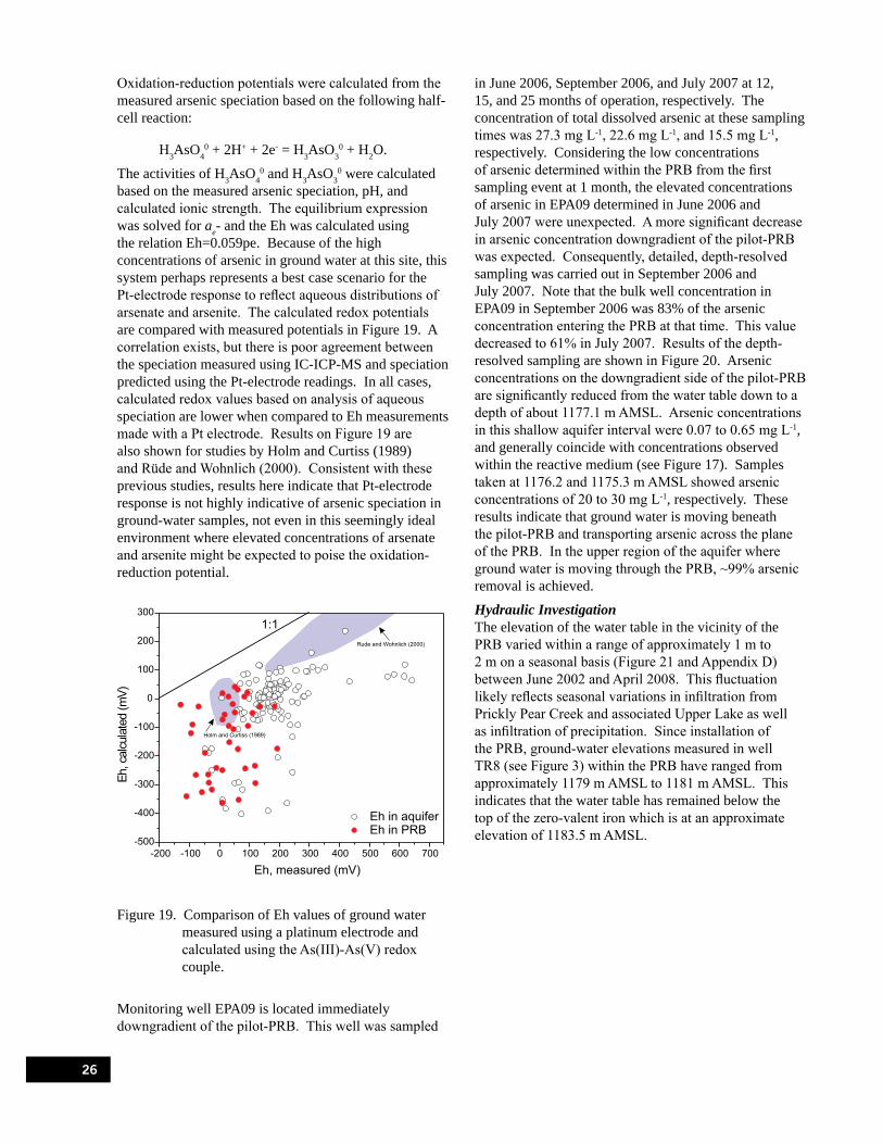
H AsO 0 + 2H+ + 2e- = H AsO 0 + H O.3 4 3 3 2

Oxidation-reduction potentials were calculated from the measured arsenic speciation based on the following half-cell reaction:

The activities of H AsO 0 and H AsO 0 were calculated3 4 3 3 based on the measured arsenic speciation, pH, and calculated ionic strength. The equilibrium expression was solved for ae- and the Eh was calculated using the relation Eh=0.059pe. Because of the high concentrations of arsenic in ground water at this site, this system perhaps represents a best case scenario for the Pt-electrode response to reflect aqueous distributions of arsenate and arsenite. The calculated redox potentials are compared with measured potentials in Figure 19. A correlation exists, but there is poor agreement between the speciation measured using IC-ICP-MS and speciation predicted using the Pt-electrode readings. In all cases, calculated redox values based on analysis of aqueous speciation are lower when compared to Eh measurements made with a Pt electrode. Results on Figure 19 are also shown for studies by Holm and Curtiss (1989) and Rüde and Wohnlich (2000). Consistent with these previous studies, results here indicate that Pt-electrode response is not highly indicative of arsenic speciation in ground-water samples, not even in this seemingly ideal environment where elevated concentrations of arsenate and arsenite might be expected to poise the oxidation-reduction potential.

Figure 19. Comparison of Eh values of ground water measured using a platinum electrode and calculated using the As(III)-As(V) redox couple.

Monitoring well EPA09 is located immediately downgradient of the pilot-PRB. This well was sampled

in June 2006, September 2006, and July 2007 at 12, 15, and 25 months of operation, respectively. The concentration of total dissolved arsenic at these sampling times was 27.3 mg L-1, 22.6 mg L-1, and 15.5 mg L-1, respectively. Considering the low concentrations of arsenic determined within the PRB from the first sampling event at 1 month, the elevated concentrations of arsenic in EPA09 determined in June 2006 and July 2007 were unexpected. A more significant decrease in arsenic concentration downgradient of the pilot-PRB was expected. Consequently, detailed, depth-resolved sampling was carried out in September 2006 and July 2007. Note that the bulk well concentration in EPA09 in September 2006 was 83% of the arsenic concentration entering the PRB at that time. This value decreased to 61% in July 2007. Results of the depth-resolved sampling are shown in Figure 20. Arsenic concentrations on the downgradient side of the pilot-PRB are significantly reduced from the water table down to a depth of about 1177.1 m AMSL. Arsenic concentrations in this shallow aquifer interval were 0.07 to 0.65 mg L-1, and generally coincide with concentrations observed within the reactive medium (see Figure 17). Samples taken at 1176.2 and 1175.3 m AMSL showed arsenic concentrations of 20 to 30 mg L-1, respectively. These results indicate that ground water is moving beneath the pilot-PRB and transporting arsenic across the plane of the PRB. In the upper region of the aquifer where ground water is moving through the PRB, ~99% arsenic removal is achieved.

Hydraulic Investigation The elevation of the water table in the vicinity of the PRB varied within a range of approximately 1 m to 2 m on a seasonal basis (Figure 21 and Appendix D) between June 2002 and April 2008. This fluctuation likely reflects seasonal variations in infiltration from Prickly Pear Creek and associated Upper Lake as well as infiltration of precipitation. Since installation of the PRB, ground-water elevations measured in well TR8 (see Figure 3) within the PRB have ranged from approximately 1179 m AMSL to 1181 m AMSL. This indicates that the water table has remained below the top of the zero-valent iron which is at an approximate elevation of 1183.5 m AMSL.

26

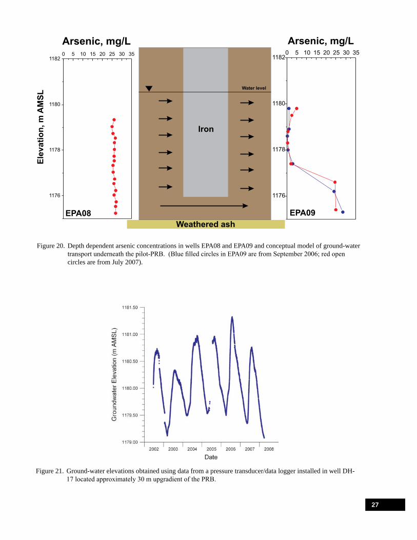
Figure 20. Depth dependent arsenic concentrations in wells EPA08 and EPA09 and conceptual model of ground-water transport underneath the pilot-PRB. (Blue filled circles in EPA09 are from September 2006; red open circles are from July 2007).

Figure 21. Ground-water elevations obtained using data from a pressure transducer/data logger installed in well DH­17 located approximately 30 m upgradient of the PRB.

27

Temporal variations in the potentiometric surface near the PRB were interpreted from data obtained by manual measurements of ground-water elevations on nine dates between July 2005 and June 2008. Based on these data, there is no evidence of ground-water mounding upgradient of the PRB that would indicate the PRB is acting as a significant impediment to ground-water flow. The surfaces (Appendix E) were similar

to that interpreted from data obtained on April 1, 2008 (Figure 22), indicating that the hydraulic gradient was relatively stable in both magnitude and direction through time. In each case, the data indicated a northwest direction of flow. The magnitude of the hydraulic gradient near the PRB ranged from approximately 0.005 to 0.008 with an average of 0.006.

Figure 22. Shallow potentiometric surface interpreted from ground-water elevation measurements obtained using an electronic water level indicator on April 1, 2008. The contour interval between equipotential lines is 0.1 m. The approximate location of the PRB is depicted in red.

To better evaluate the full range of variation in hydraulic gradient potentially associated with seasonal changes in ground-water elevations, data obtained from pressure transducers/data loggers installed in wells DH-17, PBTW-2, and EPA06 (Figure 23) were used to estimate the direction and magnitude of the gradient approximately every four hours between July 2005 and April 2008. The estimated magnitude and direction

of the gradient were averaged on a daily basis. The magnitude of the gradient calculated from this expanded data set also ranged from approximately 0.005 to 0.008 (Figure 24) with an average of 0.006. The estimated direction of ground-water flow ranged from an azimuth of 322 deg to 350 deg (Figure 23) with an average azimuth of 334 deg.

28

Figure 23. Wells instrumented with pressure transducers/data loggers and used to characterize hydraulic gradient fluctuations on a daily basis. The azimuthal distribution in degrees of the calculated hydraulic gradient vectors is depicted using a Rose diagram in the figure inset. Locations of the wells and approximate location of the PRB (red line) are overlain on the potentiometric surface on April 1, 2008, for reference. The contour interval between equipotential lines is 0.1 m.

A natural gradient tracer test was performed from June 23 to 29, 2008, using a solution of potable water amended with sodium bromide to provide another direct line of evidence verifying ground-water flow through the PRB. A slug of approximately 95 L of potable water with a bromide ion concentration of approximately 500 mg L-1 was injected into well TR1 (Figure 25) over a period of approximately 5 min. The injection was restricted to a 0.9 m zone between approximately 1177.4 m and 1178.3 m AMSL by isolating this zone with mechanical packers. The injection pipe consisted of hand perforated 3/4” Schedule 40 PVC.

Figure 24. Distribution of the magnitude of the hydraulic gradient near the PRB estimated on a daily basis using data obtained from pressure transducers/data loggers installed in wells DH-17, PBTW-2, and EPA06.

29

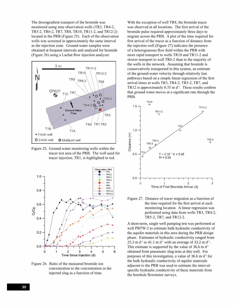
The downgradient transport of the bromide was monitored using nine observation wells (TR3, TR4-2, TR5-2, TR6-2, TR7, TR8, TR10, TR11-2, and TR12-2) located in the PRB (Figure 25). Each of the observation wells was screened in approximately the same interval as the injection zone. Ground-water samples were obtained at frequent intervals and analyzed for bromide (Figure 26) using a Lachat flow injection analyzer.

Figure 25. Ground-water monitoring wells within the tracer test area of the PRB. The well used for tracer injection, TR1, is highlighted in red.

Figure 26. Ratio of the measured bromide ion concentration to the concentration in the injected slug as a function of time.

With the exception of well TR8, the bromide tracer was observed at all locations. The first arrival of the bromide pulse required approximately three days to migrate across the PRB. A plot of the time required for first arrival of the tracer as a function of distance from the injection well (Figure 27) indicates the presence of a heterogeneous flow field within the PRB with more rapid transport to wells TR10 and TR11-2 and slower transport to well TR6-2 than to the majority of the wells in the network. Assuming that bromide is conservatively transported in this system, an estimate of the ground-water velocity through relatively fast pathways based on a simple linear regression of the first arrival times at wells TR3, TR4-2, TR5-2, TR7, and TR12 is approximately 0.35 m d-1. These results confirm that ground water moves at a significant rate through the PRB.

Figure 27. Distance of tracer migration as a function of the time required for the first arrival at each monitoring location. A linear regression was performed using data from wells TR3, TR4-2, TR5-2, TR7, and TR12-2.

A short-term, single well pumping test was performed at well PBTW-2 to estimate bulk hydraulic conductivity of the aquifer materials in this area during the PRB design phase. Estimates of hydraulic conductivity ranged from 25.3 m d-1 to 41.1 m d-1 with an average of 33.2 m d-1. This estimate is supported by the value of 36.6 m d-1

obtained from pneumatic slug tests at this well. For purposes of this investigation, a value of 36.6 m d-1 for the bulk hydraulic conductivity of aquifer materials adjacent to the PRB was used to estimate the interval-specific hydraulic conductivity of these materials from the borehole flowmeter surveys.

30

Results of pneumatic slug tests performed in short (0.76 m) screened wells located within the PRB (Table 5, Figure 28) ranged from 2.1 m d-1 to 110 m d-1 with an average of approximately 58 m d-1. The highest estimates for the hydraulic conductivity of the PRB were consistently obtained from wells screened below approximately 1177.4 m AMSL. No changes were observed in the distribution of hydraulic conductivity between measurements made after 5 months and after 16 months (Figure 29). Pneumatic slug tests were also performed in July 2007 in two wells, TR1 and EPA10, that screen the majority of the PRB and are located (see Figure 3) near the western end and center of the PRB, respectively. Results indicate the average hydraulic conductivity of materials adjacent to these wells is approximately 43 m d-1 (well TR1) and 49 m d-1

(well EPA10). It is noted that the majority of these values are equal to or significantly greater than the permeability estimated for a sample of the zerovalent iron material (30 m d-1 to 58 m d-1) using laboratory test method ASTM 2434 during the PRB design phase. This indicates that the PRB installation method did not significantly reduce the hydraulic conductivity of the PRB materials.

Table 5. Estimates of hydraulic conductivity in units of m d-1 obtained from pneumatic slug tests performed in wells located within the PRB.

Well October 2005

September 2006 July 2007

EPA10 49

S01 88

S02 75

S03 98 98

S04 7.3 11

S05 56 42

S06 100 110

S07 95 92

S08 70 69

TR1 32 43

TR2 55

TR3 51

TR7 43

TR8 47

TR9 2.1

TR10 34

The borehole flowmeter methodology has been used to characterize the hydraulic conductivity of aquifer materials adjacent to six wells (PBTW-1, PBTW-2, DH-17, EPA02, EPA08, EPA09, and EPA10) (Figure 3). With the exception of existing well DH-17, each of these wells is screened from approximately the water table to the top of the ash unit underlying the upper aquifer. Three of the wells bound the study area to the east (PBTW-1 and PBTW-2) and south (DH-17), providing information concerning the scale of heterogeneity in this portion of the site. At well PBTW-1 (Figure 30), aquifer materials immediately above the ash unit at the bottom of the well screen appear to have higher hydraulic conductivity than the average for materials in this portion of the site.

31

Figure 28. Results of pneumatic slug tests within the PRB using a series of wells each screening a 0.76 m vertical interval. The screened elevations are depicted by the length of the line representing each well. The results of laboratory permeameter measurements of the zero-valent iron used in construction of the PRB are provided for reference.

32

Figure 29. Results of pneumatic slug tests within the PRB after 5 months and 16 months.

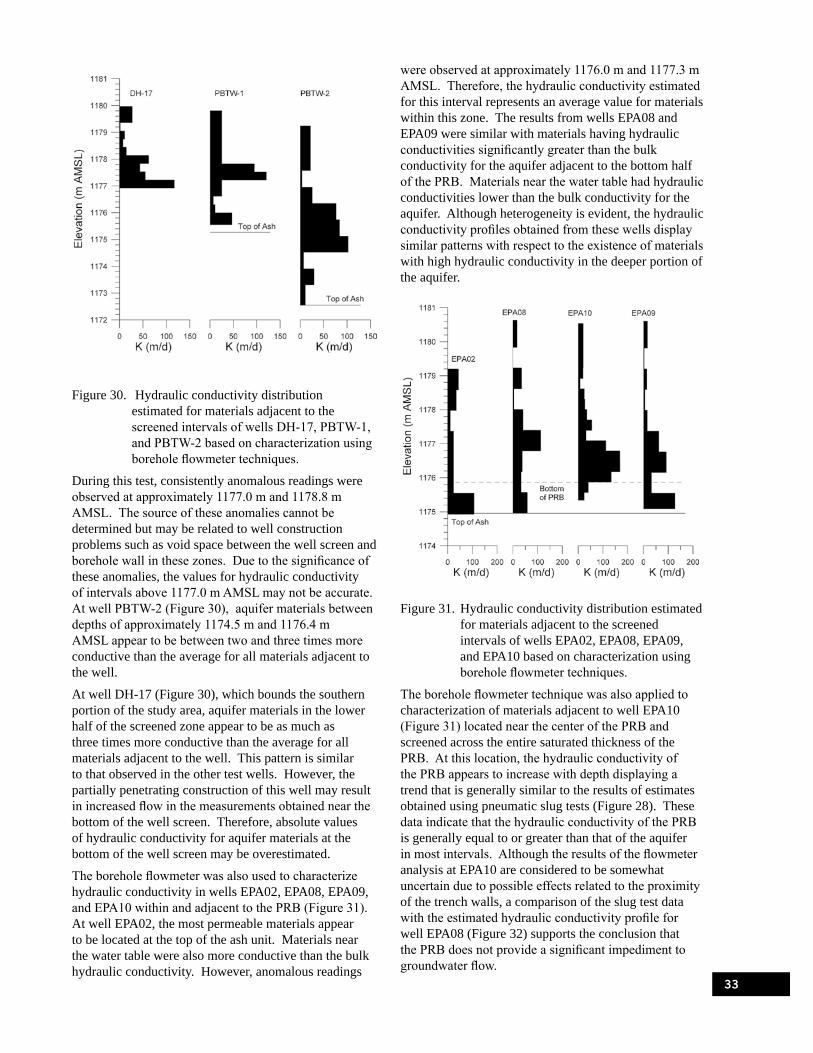
Figure 30. Hydraulic conductivity distribution estimated for materials adjacent to the screened intervals of wells DH-17, PBTW-1, and PBTW-2 based on characterization using borehole flowmeter techniques.

During this test, consistently anomalous readings were observed at approximately 1177.0 m and 1178.8 m AMSL. The source of these anomalies cannot be determined but may be related to well construction problems such as void space between the well screen and borehole wall in these zones. Due to the significance of these anomalies, the values for hydraulic conductivity of intervals above 1177.0 m AMSL may not be accurate. At well PBTW-2 (Figure 30), aquifer materials between depths of approximately 1174.5 m and 1176.4 m AMSL appear to be between two and three times more conductive than the average for all materials adjacent to the well.

At well DH-17 (Figure 30), which bounds the southern portion of the study area, aquifer materials in the lower half of the screened zone appear to be as much as three times more conductive than the average for all materials adjacent to the well. This pattern is similar to that observed in the other test wells. However, the partially penetrating construction of this well may result in increased flow in the measurements obtained near the bottom of the well screen. Therefore, absolute values of hydraulic conductivity for aquifer materials at the bottom of the well screen may be overestimated.

The borehole flowmeter was also used to characterize hydraulic conductivity in wells EPA02, EPA08, EPA09, and EPA10 within and adjacent to the PRB (Figure 31). At well EPA02, the most permeable materials appear to be located at the top of the ash unit. Materials near the water table were also more conductive than the bulk hydraulic conductivity. However, anomalous readings

were observed at approximately 1176.0 m and 1177.3 m AMSL. Therefore, the hydraulic conductivity estimated for this interval represents an average value for materials within this zone. The results from wells EPA08 and EPA09 were similar with materials having hydraulic conductivities significantly greater than the bulk conductivity for the aquifer adjacent to the bottom half of the PRB. Materials near the water table had hydraulic conductivities lower than the bulk conductivity for the aquifer. Although heterogeneity is evident, the hydraulic conductivity profiles obtained from these wells display similar patterns with respect to the existence of materials with high hydraulic conductivity in the deeper portion of the aquifer.

Figure 31. Hydraulic conductivity distribution estimated for materials adjacent to the screened intervals of wells EPA02, EPA08, EPA09, and EPA10 based on characterization using borehole flowmeter techniques.

The borehole flowmeter technique was also applied to characterization of materials adjacent to well EPA10 (Figure 31) located near the center of the PRB and screened across the entire saturated thickness of the PRB. At this location, the hydraulic conductivity of the PRB appears to increase with depth displaying a trend that is generally similar to the results of estimates obtained using pneumatic slug tests (Figure 28). These data indicate that the hydraulic conductivity of the PRB is generally equal to or greater than that of the aquifer in most intervals. Although the results of the flowmeter analysis at EPA10 are considered to be somewhat uncertain due to possible effects related to the proximity of the trench walls, a comparison of the slug test data with the estimated hydraulic conductivity profile for well EPA08 (Figure 32) supports the conclusion that the PRB does not provide a significant impediment to groundwater flow.

33

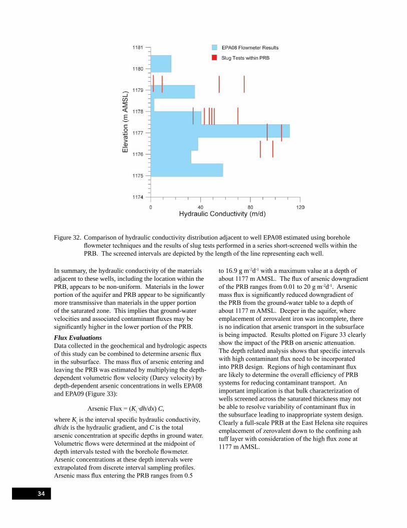
Figure 32. Comparison of hydraulic conductivity distribution adjacent to well EPA08 estimated using borehole flowmeter techniques and the results of slug tests performed in a series short-screened wells within the PRB. The screened intervals are depicted by the length of the line representing each well.

In summary, the hydraulic conductivity of the materials adjacent to these wells, including the location within the PRB, appears to be non-uniform. Materials in the lower portion of the aquifer and PRB appear to be significantly more transmissive than materials in the upper portion of the saturated zone. This implies that ground-water velocities and associated contaminant fluxes may be significantly higher in the lower portion of the PRB.

Flux Evaluations Data collected in the geochemical and hydrologic aspects of this study can be combined to determine arsenic flux in the subsurface. The mass flux of arsenic entering and leaving the PRB was estimated by multiplying the depth-dependent volumetric flow velocity (Darcy velocity) by depth-dependent arsenic concentrations in wells EPA08 and EPA09 (Figure 33):

Arsenic Flux = (Ki ·dh/dx) C,

where Ki is the interval specific hydraulic conductivity, dh/dx is the hydraulic gradient, and C is the total arsenic concentration at specific depths in ground water. Volumetric flows were determined at the midpoint of depth intervals tested with the borehole flowmeter. Arsenic concentrations at these depth intervals were extrapolated from discrete interval sampling profiles. Arsenic mass flux entering the PRB ranges from 0.5

to 16.9 g m-2d-1 with a maximum value at a depth of about 1177 m AMSL. The flux of arsenic downgradient of the PRB ranges from 0.01 to 20 g m-2d-1. Arsenic mass flux is significantly reduced downgradient of the PRB from the ground-water table to a depth of about 1177 m AMSL. Deeper in the aquifer, where emplacement of zerovalent iron was incomplete, there is no indication that arsenic transport in the subsurface is being impacted. Results plotted on Figure 33 clearly show the impact of the PRB on arsenic attenuation. The depth related analysis shows that specific intervals with high contaminant flux need to be incorporated into PRB design. Regions of high contaminant flux are likely to determine the overall efficiency of PRB systems for reducing contaminant transport. An important implication is that bulk characterization of wells screened across the saturated thickness may not be able to resolve variability of contaminant flux in the subsurface leading to inappropriate system design. Clearly a full-scale PRB at the East Helena site requires emplacement of zerovalent down to the confining ash tuff layer with consideration of the high flux zone at 1177 m AMSL.

34

Figure 33. Estimation of arsenic flux entering and leaving the PRB as a function of depth.

PRB Performance A number of factors have been shown to be important in controlling the long-term performance of zerovalent iron reactive barriers. Key among these factors are reaction processes that lead to excessive oxidative corrosion of iron granules and/or excessive carbonate mineral precipitation (e.g., U.S. EPA, 2003a, Liang et al., 2005; Li et al., 2006). Both of these processes degrade the reactive and hydraulic performance of zerovalent iron PRBs. Dissolved oxygen (DO), for example, rapidly reacts with zerovalent iron and drives the formation of various ferric oxide, oxyhydroxide, and hydroxide minerals. In situations where ground water containing several mg L-1 of DO interacts with zerovalent iron, rapid cementation and loss of pore space and hydraulic conductivity occurs due to the precipitation of ferric-iron bearing minerals. Although the formation of these Fe(III) corrosion products may be a benefit from the standpoint of arsenic removal (e.g., Furukawa et al., 2002), excessive corrosion can lead to the complete bypass of the reactive medium. This particular problem is not a concern at the East Helena Site. As noted above DO concentrations entering the PRB are very low and core samples show no evidence of nodule formation or cementation after 15 months of operation.

Carbonate mineral precipitation in PRBs is primarily driven by the pH increase that comes about during anaerobic corrosion of metallic iron. Typically ground water is saturated or undersaturated with respect to calcium carbonate phases (e.g., calcite and aragonite); however, as ground-water pH increases, saturation with respect to various carbonate minerals is approached and is usually exceeded at pH>9. This situation drives precipitation of fairly low density minerals that over time can impact the performance of PRBs by decreasing

reactivity (by coating iron surfaces and removing reactive sites) and decreasing porosity and permeability and thereby affecting hydraulic performance (U.S. EPA, 2003a; Li et al., 2006). Geochemical modeling results indicate that ground water upgradient of the PRB is saturated to near-saturated with aragonite (CaCO3; Figure 34). Ground water within the PRB is slightly oversaturated with respect to aragonite at pH>8. These model results and the observed decrease in calcium concentrations between upgradient and in-wall sampling points suggest that precipitation of aragonite is occurring in the PRB. However, ground water entering the PRB is sodium-sulfate type water (see Figure 10 and discussion above). Concentrations of calcium and bicarbonate are comparatively low (~50 mg L-1 and 200 mg L-1, respectively) in the influent ground water. Consequently, rapid buildup of carbonate phases is not expected. Measurements of inorganic carbon concentrations accumulated on the reactive medium after 15 months range from 0.01 to 0.46 wt% (mean 0.09 wt%, n=29, Figure 35), with the highest values observed near the leading edge of the barrier and at shallow depths where pH is elevated. The maximum carbonate concentration observed after 15 months corresponds to an equivalent reduction in the fractional porosity of <0.05 (U.S. EPA, 2003a).

Figure 34. Aragonite saturation indices in ground water as a function of pH upgradient and within the PRB.

35

Figure 35. Solid-phase concentrations of inorganic carbon, sulfur, and arsenic in PRB core materials.

Elevated concentrations of sulfate (~530 mg L-1) in ground water entering the PRB coupled with moderately to highly reducing conditions in the PRB have led to the reduction of sulfate and production of sulfide, which has precipitated in the PRB, likely as an iron sulfide. Evidence for sulfate reduction in the PRB includes decreases in sulfate concentrations (up to 100%; Figure 36), detection of dissolved sulfide within and downgradient of the PRB (up to 13 mg L-1), and accumulation of sulfur on the reactive medium. Reduction in sulfate concentrations is greatest at shallower depths where residence time in the PRB is the greatest (Figure 36 inset). Total sulfur values determined in core samples range from 100 to 1200 mg kg-1 (mean 400 mg kg-1, n=43, Figure 35). Previous studies have shown that sulfur accumulation in zerovalent iron PRBs is mainly due to precipitation of mackinawite (FeS, e.g., Roh et al., 2000; Furukawa et al., 2002; Wilkin et al., 2003). The sulfate reduction process is microbially mediated. Sulfate-reducing bacteria in this system utilize either hydrogen (formed during the anaerobic iron corrosion) or possibly organic carbon (derived from broken-down guar gum), or both. Column and batch experiments performed during the design phase of the study were abiotic; sulfate was present in the systems but behaved as a conservative tracer and was not reduced to sulfide. Consequently this important aspect of PRB behavior is typically not captured in laboratory experimentation (but see Nooten et al., 2008).

Figure 36. Sulfate removal within the PRB as a function of time and depth. Sulfate concentration entering the PRB, C0, is 530 mg L-1.

The role of arsenic-sulfur interactions in zerovalent iron systems has been previously noted by Ramaswami et al. (2001), Nikolaidis et al. (2003), and Köber et al. (2005). Reduction of sulfate to sulfide can impact: 1) the aqueous speciation of arsenic by driving the formation of thioarsenic species and, 2) the removal process of arsenic in the reactive medium. Aqueous thioarsenic formation was noted within the PRB in several wells with sulfide concentrations above 0.2 mg L-1. Figure 37 shows an IC-ICP-MS chromatogram for ground water from influent well EPA08 and PRB well TR9. As noted previously, arsenite dominates the aqueous speciation of arsenic in influent ground water. In well TR9, the dissolved arsenic and sulfide concentrations were 0.38 mg L-1 and 0.42 mg L-1, respectively. Arsenite is present in trace amounts. Note that the arsenate concentration in TR9 is similar to the influent and two additional As-S species are present. The additional species are thioarsenic ions that contain S and As in the ratio of 1:1 and 2:1, respectively (Figure 37).

36

Figure 37. Chromatograph of arsenic speciation for ground water entering the PRB (well EPA08) and ground water from well TR9 containing thioarsenic species.

Because arsenic and sulfur form bonded ions in the aqueous phase, it is reasonable to expect solid-phase associations of arsenic and sulfur in the reactive medium. The nature of arsenic bonding in the solid-phase is examined in a following section describing x-ray absorption spectroscopy results. The problem is explored here with the aid of geochemical modeling. Removal of arsenic via the precipitation of an As(III)-bearing phase is considered on Figure 38 showing the pH-dependent solubility of As2O3 and As2S3. Claudetite (As2O3) is highly soluble and this phase is not expected to play a role in arsenic removal. Solubility of orpiment (As2S3) is highly pH dependent and influenced by the concentration of dissolved sulfide at pH<10. Based on solubility reasoning, at pH>8 it is unlikely that precipitation of As2S3 is an important arsenic removal mechanism in zerovalent iron PRBs (Köber et al., 2005). However, at lower pH it is possible that orpiment precipitation could play a role in arsenic uptake. This modeling does not rule out arsenic sorption to iron monosulfides or thioarsenic sorption to iron corrosion products (e.g., Gallegos et al., 2007; Wolthers et al., 2005). Removal of arsenate via precipitation of calcium and ferrous salts is examined on Figure 39. Note the contrasting pH dependencies of arsenite and arsenate precipitation. Arsenate removal is favored with increasing pH, whereas arsenite is expected to become increasingly more soluble at higher pH. Although there is some uncertainty in the thermodynamic data for symplesite (ferrous arsenate), the modeling results suggest that symplesite, Fe3(AsO4)2·8H2O, may precipitate in the PRB at typical conditions.

Figure 38. Solubility of As(III) phases as a function of pH and dissolved sulfide concentration. Data points are measured As(III) concentrations within the PRB.

Figure 39. Solubility of As(V) phases as a function of pH. Data points are measured As(V) concentrations within the PRB (blue circles, Fe=0.1 mM; red circles, Fe=10 µm; green circles, Fe=1 µm).

Arsenic is obviously the main contaminant of concern for which the PRB performance is critical at this site. Several other metals are present in the ground water entering the PRB, including Zn (2300 µg L-1), Cd (50 µg L-1), Co (20 µg L-1), and Ni (10 µg L-1).

Concentrations of Cd, Co, and Ni within ground water from the PRB are below detection (generally < 1 µg L-1), and Zn concentrations have decreased to <50 µg L-1. All of these metals form insoluble precipitates with sulfide, so that metal sulfide precipitation is one possible removal mechanism for these contaminants, as is adsorption onto iron corrosion products.

37

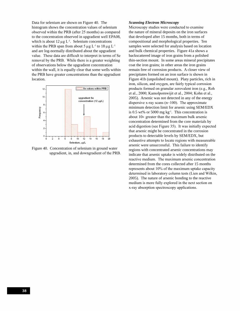
Data for selenium are shown on Figure 40. The histogram shows the concentration values of selenium observed within the PRB (after 25 months) as compared to the concentration observed in upgradient well EPA08, which is about 12 µg L-1. Selenium concentrations within the PRB span from about 5 µg L-1 to 18 µg L-1

and are log-normally distributed about the upgradient value. These data are difficult to interpret in terms of Se removal by the PRB. While there is a greater weighting of observations below the upgradient concentration within the wall, it is equally clear that some wells within the PRB have greater concentrations than the upgradient location.

Figure 40. Concentration of selenium in ground water upgradient, in, and downgradient of the PRB.

Scanning Electron Microscopy Microscopy studies were conducted to examine the nature of mineral deposits on the iron surfaces that developed after 15 months, both in terms of compositional and morphological properties. Ten samples were selected for analysis based on location and bulk chemical properties. Figure 41a shows a backscattered image of iron grains from a polished thin-section mount. In some areas mineral precipitates coat the iron grains; in other areas the iron grains remain free of corrosion products. A closer view of precipitates formed on an iron surface is shown in Figure 41b (unpolished mount). Platy particles, rich in iron, silicon, and oxygen, are fairly typical corrosion products formed on granular zerovalent iron (e.g., Roh et al., 2000; Kamolpornwijit et al., 2004; Kohn et al., 2005). Arsenic was not detected in any of the energy dispersive x-ray scans (n~100). The approximate minimum detection limit for arsenic using SEM/EDX is 0.5 wt% or 5000 mg kg-1. This concentration is about 10× greater than the maximum bulk arsenic concentration determined from the core materials by acid digestion (see Figure 35). It was initially expected that arsenic might be concentrated in the corrosion products to detectable levels by SEM/EDX, but exhaustive attempts to locate regions with measureable arsenic were unsuccessful. This failure to identify regions with concentrated arsenic concentrations may indicate that arsenic uptake is widely distributed on the reactive medium. The maximum arsenic concentration determined from the cores collected after 15 months represents about 10% of the maximum uptake capacity determined in laboratory column tests (Lien and Wilkin, 2005). The nature of arsenic bonding to the reactive medium is more fully explored in the next section on x-ray absorption spectroscopy applications.

38

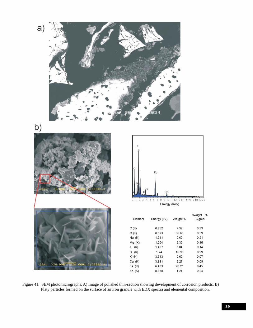
Figure 41. SEM photomicrographs. A) Image of polished thin-section showing development of corrosion products. B) Platy particles formed on the surface of an iron granule with EDX spectra and elemental composition.

39

X-ray Absorption Spectroscopy XANES analysis was conducted on reference materials, PRB core samples, source zone materials, and well boring samples collected in the aquifer near the location of the pilot-PRB. These analyses were conducted to determine the oxidation state and bonding environment of arsenic in these different environments.

XANES spectra for the reference materials are shown on Figure 42 and the corresponding absorption edge and white-line positions are listed in Table 2. Reference materials were used to analyze XANES spectra of the

unknown samples shown on Figure 43. Examination of Figure 43 indicates no contribution of elemental arsenic to any of the unknown samples. For this reason the reference line for elemental arsenic has been removed from Figure 43. Panels A and B show XANES data for PRB core materials collected in September 2006. Panel C shows XANES data for cores taken near the arsenic source zone in August 2006, and Panel D provides data for well borings collected prior to installation of the PRB in November 2004.

Figure 42. Normalized XANES spectra for arsenic reference materials used for the XANES analysis and LCF fitting of unknown samples. (A) is the absorption edge position for elemental As (11866.7 eV); (B) is the absorption edge position for As(III)-S bonds (11868.7 eV); (C) is the absorption edge position for As(III)-O bonds or As(V)-S bonds (~11870.1 eV); and, (D) is the absorption edge position for As(V)-O bonds (11874.0 eV). Orpiment (As2S3) is used as a model As(III)-S compound; FeS is disordered mackinawite (FeS); enargite (Cu3AsS4) is used as a model As(V)-S compound and scorodite (FeAsO4) is used as a model for As(V)-O.

40

Figure 43. Normalized XANES spectra for unknown samples from the ASARCO Smelter site. PRB core sample spectra are shown in Panels A (shallow depths) and B (deep depths). Panel C shows spectra for samples collected from the source zone and Panel D shows spectra of samples from a well boring taken prior to installation of the PRB. (a) is the white-line position for As(III)-S, (b) is the white-line for the As(III)-O, and (c) is the white-line position for the As(V)-O.

XANES spectra from the PRB samples show that there are multiple solid-phase arsenic species present. Arsenic in all the PRB samples includes at least two species: As(III)-O and As(V)-O, but in many samples As(III)-S appears to be present as well. It should be noted that As(V)-S cannot be ruled out in any of the samples because the As(III)-O and As(V)-S white line positions overlap (Beak et al., 2008), although this solid-phase coordination is considered to be unlikely in this environment. The source zone samples appear to contain only As(V)-O. The presence of As(III) oxyanions in the source zone ground water suggests the possibility of microbial reduction of arsenate to arsenite in the subsurface.

Multiple arsenic species are also present in well borings collected from the aquifer near the location of the pilot-PRB. In shallow samples the speciation appears to be an unusual mixture of As(V)-O and As(III)-S (Figure 43a). To our knowledge this unique arsenic speciation has not been observed in other subsurface environments. However, the observed As(III)-S speciation can be explained by the presence of a petroleum hydrocarbon plume that induces microbially mediated redox reactions. Degradation of the hydrocarbon leads to local iron- and sulfate-reducing conditions that result in the formation of Fe-S surfaces and As(III)-S speciation at shallow depths. Deeper in the aquifer, arsenic speciation is a more typical mixture

41

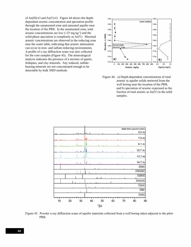
of As(III)-O and As(V)-O. Figure 44 shows the depth-dependent arsenic concentration and speciation profile through the unsaturated zone and saturated aquifer near the location of the PRB. In the unsaturated zone, total arsenic concentrations are low (<25 mg kg-1) and the solid-phase speciation is completely as As(V). Maximal arsenic concentrations are observed in the reducing zone near the water table, indicating that arsenic attenuation can occur in iron- and sulfate-reducing environments. A profile of x-ray diffraction scans was also collected for the core samples (Figure 45). The mineralogical analysis indicates the presence of a mixture of quartz, feldspars, and clay minerals. Any reduced, sulfide-bearing minerals are not concentrated enough to be detectable by bulk XRD methods.

arsenic in aquifer solids retrieved from the well boring near the location of the PRB, and b) speciation of arsenic expressed as the fraction of total arsenic as As(V) in the solid samples.

Figure 44. a) Depth-dependent concentrations of total

42

Figure 45. Powder x-ray diffraction scans of aquifer materials collected from a well boring taken adjacent to the pilot-PRB.

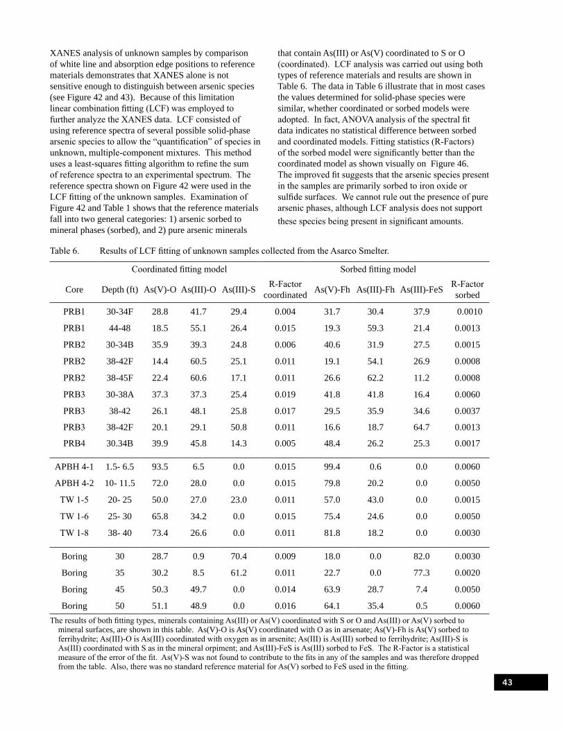
XANES analysis of unknown samples by comparison of white line and absorption edge positions to reference materials demonstrates that XANES alone is not sensitive enough to distinguish between arsenic species (see Figure 42 and 43). Because of this limitation linear combination fitting (LCF) was employed to further analyze the XANES data. LCF consisted of using reference spectra of several possible solid-phase arsenic species to allow the “quantification” of species in unknown, multiple-component mixtures. This method uses a least-squares fitting algorithm to refine the sum of reference spectra to an experimental spectrum. The reference spectra shown on Figure 42 were used in the LCF fitting of the unknown samples. Examination of Figure 42 and Table 1 shows that the reference materials fall into two general categories: 1) arsenic sorbed to mineral phases (sorbed), and 2) pure arsenic minerals

that contain As(III) or As(V) coordinated to S or O (coordinated). LCF analysis was carried out using both types of reference materials and results are shown in Table 6. The data in Table 6 illustrate that in most cases the values determined for solid-phase species were similar, whether coordinated or sorbed models were adopted. In fact, ANOVA analysis of the spectral fit data indicates no statistical difference between sorbed and coordinated models. Fitting statistics (R-Factors) of the sorbed model were significantly better than the coordinated model as shown visually on Figure 46. The improved fit suggests that the arsenic species present in the samples are primarily sorbed to iron oxide or sulfide surfaces. We cannot rule out the presence of pure arsenic phases, although LCF analysis does not support these species being present in significant amounts.

Table 6. Results of LCF fitting of unknown samples collected from the Asarco Smelter.

Core

Coordinated fitting model

Depth (ft) As(V)-O As(III)-O As(III)-S R-Factor coordinated

Sorbed fitting model

As(V)-Fh As(III)-Fh As(III)-FeS R-Factor sorbed

PRB1

PRB1

PRB2

PRB2

PRB2

PRB3

PRB3

PRB3

PRB4

30-34F

44-48

30-34B

38-42F

38-45F

30-38A

38-42

38-42F

30.34B

28.8

18.5

35.9

14.4

22.4

37.3

26.1

20.1

39.9

41.7

55.1

39.3

60.5

60.6

37.3

48.1

29.1

45.8

29.4

26.4

24.8

25.1

17.1

25.4

25.8

50.8

14.3

0.004

0.015

0.006

0.011

0.011

0.019

0.017

0.011

0.005

31.7

19.3

40.6

19.1

26.6

41.8

29.5

16.6

48.4

30.4

59.3

31.9

54.1

62.2

41.8

35.9

18.7

26.2

37.9

21.4

27.5

26.9

11.2

16.4

34.6

64.7

25.3

0.0010

0.0013

0.0015

0.0008

0.0008

0.0060

0.0037

0.0013

0.0017

APBH 4-1

APBH 4-2

TW 1-5

TW 1-6

TW 1-8

1.5- 6.5

10- 11.5

20- 25

25- 30

38- 40

93.5

72.0

50.0

65.8

73.4

6.5

28.0

27.0

34.2

26.6

0.0

0.0

23.0

0.0

0.0

0.015

0.015

0.011

0.015

0.011

99.4

79.8

57.0

75.4

81.8

0.6

20.2

43.0

24.6

18.2

0.0

0.0

0.0

0.0

0.0

0.0060

0.0050

0.0015

0.0050

0.0030

Boring

Boring

Boring

Boring

30

35

45

50

28.7

30.2

50.3

51.1

0.9

8.5

49.7

48.9

70.4

61.2

0.0

0.0

0.009

0.011

0.014

0.016

18.0

22.7

63.9

64.1

0.0

0.0

28.7

35.4

82.0

77.3

7.4

0.5

0.0030

0.0020

0.0050

0.0060 The results of both fitting types, minerals containing As(III) or As(V) coordinated with S or O and As(III) or As(V) sorbed to

mineral surfaces, are shown in this table. As(V)-O is As(V) coordinated with O as in arsenate; As(V)-Fh is As(V) sorbed to ferrihydrite; As(III)-O is As(III) coordinated with oxygen as in arsenite; As(III) is As(III) sorbed to ferrihydrite; As(III)-S is As(III) coordinated with S as in the mineral orpiment; and As(III)-FeS is As(III) sorbed to FeS. The R-Factor is a statistical measure of the error of the fit. As(V)-S was not found to contribute to the fits in any of the samples and was therefore dropped from the table. Also, there was no standard reference material for As(V) sorbed to FeS used in the fitting.

43

Figure 46. Comparison of LCF fitting results using a) coordinated or b) sorbed reference materials for PRB core sample Core 1 30-34F. The solid black line is the measured spectra and the open red circles are the fits.

Keeping the previous discussion in mind and using the LCF and XANES data we can make some generalizations about the speciation of arsenic in the solid samples collected from the source zone, aquifer adjacent to the PRB, and the PRB. A ternary diagram is shown in Figure 47 that shows the relative proportions of As(III)-O, As(V)-O, and As(III)-S bonding environments. In all cases the PRB core samples likely contained three species, As(V) and As(III) sorbed to Fe (oxy)hydroxides and As(III) sorbed to Fe sulfide phases. Samples collected in the source zone contained two As species As(V) and As(III) sorbed to Fe (oxy)hydroxides and in the case of sample APBH 4-1 the speciation was primarily As(V) sorbed to Fe (oxy)hydroxides, although there was a small amount of As(III) sorbed to (oxy) hydroxides. The well borings collected prior to PRB installation show that the speciation in the shallow depths was primarily As(III) sorbed to FeS, with a small fraction of the speciation being As(V) sorbed to Fe (oxy) hydroxides. Again this is likely because of hydrocarbon contamination driving microbial processes that result in iron- and sulfate-reducing conditions. Finally, in the deeper depths the speciation was As(V) and As(III) sorbed to Fe (oxy)hydroxides.

44

Figure 47. Ternary diagram showing the solid-phase arsenic speciation based on XANES LCF in samples collected from the PRB, source zone, and aquifer adjacent to the pilot-PRB.

7.0 Future Study Improvements

At this point it may be worthwhile to point out areas where this study could have been improved to help future efforts of this sort and to indicate planned continued studies. One obvious shortcoming of the study is the fact that the lower confining unit was not tagged during construction of the pilot PRB. As noted in the report, however, the negative consequences exceeded the possible benefit. More information is needed at this site regarding the continuity and thickness of the lower ash confining unit. The initial high DOC concentrations were a bit surprising and were not helpful in the early ground-water sampling campaigns. While it is possible

that microbial populations were stimulated by this dose of organic carbon, it may have been beneficial to spend more time and effort in attempts to actively degrade the residual bioslurry. Future plans involve more detailed tracer studies that combine heat and chemical tracers. Spectroscopic studies that move beyond the near-edge region of arsenic are also planned on a new set of cores to be collected after about 3.5 y of operation. These cores will be subjected to XRD analysis, as well as As EXAFS and Fe EXAFS analysis, to better fingerprint the important arsenic uptake and iron corrosion processes.

45

8.0 Summary and Relevance to Other Sites

In June 2005, a 9.1 m long, 14 m deep, and 1.8 to 2.4 m wide (in the direction of ground-water flow) pilot-scale permeable reactive barrier (PRB) was installed at a former metal smelting facility, located near Helena, Montana. The reactive barrier was installed over a 3-day period using bio-polymer slurry methods and modified excavating equipment for deep trenching. The reactive medium was composed entirely of granular iron. A monitoring network of approximately 40 ground-water sampling wells was installed in July 2005. Ground water samples were collected and analyzed at 1 month, 4 months, 12 months, 15 and 25 months of operation.

After over 2 years of monitoring, results indicate arsenic concentrations >25 mg L-1 in wells located hydraulically upgradient of the PRB. Within the PRB, arsenic concentrations are reduced to 2 to <0.01 mg L-1. Detailed studies in the aquifer downgradient of the PRB show an upper zone of the saturated aquifer (8.8 m to 12.8 m below land surface) where arsenic concentrations are reduced to <0.5 mg L-1 after 25 months of operation. Arsenic concentrations in the lower zone of the downgradient region, from 12.8 m to 14.6 m below land surface, increase with increasing depth to a maximum value of about 27 mg L-1, or roughly the same arsenic concentration observed on the upgradient side of the PRB. Ineffective treatment of arsenic over the lower depth interval is likely due to the fact that the maximum PRB depth is 13.7-14.0 m below land surface, about 1 m short of the depth of the basal weathered ash. The pilot-PRB was not anchored into the weathered ash because of uncertainties about the ash thickness in the area of the site where the PRB was installed and to insure that the lower confining unit was not breached during the excavation. In short, where hydraulic connection between the upgradient aquifer and the PRB is established, the pilot PRB is performing as expected.

Monitoring of the water table upgradient of the PRB indicates that mounding of groundwater on the leading edge of the barrier is negligible. In addition, slug testing in the PRB indicates hydraulic conductivities average approximately 60 m d-1, a value that is comparable to the native aquifer materials in this region of the site. These data, along with other geochemical indicators (such as reduced arsenic concentrations in the PRB), indicate that the system is meeting hydraulic performance expectations.

General conclusions and observations can be made regarding the application of PRB technology with granular iron for treatment of arsenic in ground water.

•Zerovalent iron can be effectively used to treat ground water contaminated with arsenic given appropriate geochemical and hydrological conditions. Results of pilot testing are promising in that significant concentration reductions for arsenic have been achieved for over 2 years in the downgradient aquifer directly impacted by the PRB and the system is meeting hydraulic performance expectations. Solid-phase tests indicate that <10% of the arsenic uptake capacity of the reactive medium was used after about 1 year of operation.

•Arsenic removal processes appear to be complex as multiple bonding and coordination environments around arsenic are revealed using advanced spectroscopic techniques. Sequestration mechanisms taking place in the field are more varied compared to those previously indicated in highly controlled laboratory tests. PRB core samples likely contain arsenic in three solid-phase species: As(V) and As(III) sorbed to Fe (oxy)hydroxides and As(III) sorbed to Fe sulfide phases. This study demonstrated a relationship between observed distributions of aqueous species of arsenic with solid-phase species as determined using spectroscopic analyses.

•Granular iron has a finite capacity to remove arsenic from solution. Therefore, successful applications of PRB technology for arsenic removal require detailed subsurface characterization data that capture geochemical and hydrogeologic variability. Evaluation of depth-dependent arsenic flux is critical. Zones with maximal contaminant flux will necessarily dictate system design requirements. This study employed discrete interval sampling for geochemical profiles, interval-specific probes of hydraulic conductivity, and continuous water level logging to evaluate long-term arsenic transport in the subsurface. Flux evaluations indicate that arsenic removal by zerovalent is highly effective at loadings below 5 g As/m2d.

•Sodium-sulfate-type ground water is better suited for contaminant treatment by zerovalent iron over calcium-bicarbonate-type ground water. Carbonate

46

precipitation is an undesirable consequence of zerovalent iron applications and is expected to reduce long-term reactive and hydraulic performance. Microbial reduction of sulfate to sulfide and precipitation of low-density iron sulfides within the reactive medium creates additional mineral surfaces for arsenic removal.

• Source control measures will reduce arsenic loading to the PRB and implementation of such measures should result in increased PRB lifetimes. The increase in effective lifetime should be directly proportional to the level of concentration reduction achieved by isolating and/or treating the source of contamination.

47

9.0 References

Bain, J., D. Blowes, D. Smyth, C. Ptacek, J. Wilkens, and R. Ludwig. “Permeable reactive barriers for the in-situ treatment of arsenic contaminated groundwater.” In Proceedings of the 5th International Conference on Remediation of Chlorinated and Recalcitrant Compounds, Battelle Press, Columbus, OH, 2006.

Bang, S., M. D. Johnson, G. P. Korfiatis, and X. Meng. Chemical reactions between arsenic and zero-valent iron in water. Water Research 39: 763-770 (2005a).

Bang, S., G. P. Korfiatis, and X. Meng. Removal of arsenic from water by zero-valent iron. Journal of Hazardous Materials 121: 61-67 (2005b).

Beak, D., R. T. Wilkin, R. G. Ford, and S. Kelly. An examination of arsenic speciation in sulfidic solutions using x-ray absorption spectroscopy. Environmental Science and Technology 42: 1643-1650 (2008).

Blowes, D. W., C. J. Ptacek, S. G. Benner, C. W. T. McRae, T. A. Bennett, and R. W. Puls. Treament of inorganic contaminants using permeable reactive barriers. Journal of Contaminant Hydrology 45: 123-137 (2000).

Biterna, M., A. Arditsoglou, E. Tsikouras, and D. Voutsa. Arsenate removal by zero valent iron: Batch and column tests. Journal of Hazardous Materials 149: 548-552 (2007).

Bouwer, H. and R. C. Rice. A slug test method for determining hydraulic conductivity of unconfined aquifers with completely or partially penetrating wells. Water Resources Research 12: 423-428 (1976).

Briar, D. W. and J. P. Madison. Hydrogeology of the Helena valley-fill aquifer system, west-central Montana. Water-Resources Investigations Report 92-4023, U.S. Geological Survey, Reston, VA, 1992.

Butler, J. J., Jr. The Design, Performance, and Analysis of Slug Tests, Lewis Publishers, Boca Raton, 1997.

Butler, J. J., Jr. and E. J. Garnett. Simple procedures for analyses of slug tests in formations of high hydraulic conductivity using spreadsheet and scientific graphics software. Kansas Geological Survey, Open File Report 2000-40, 2000.

Cherry, J. A., A. U. Shaikh, D. E. Tallman, and R. V. Nicholson. Arsenic species as an indicator of redox conditions in groundwater. Journal of Hydrology 43: 373-392 (1979).

Cullen, W. R. and K. J. Reimer. Arsenic speciation in the environment. Chemical Reviews 89: 713-764 (1989).

Del Razo, L. M., M. A. Arellano, and M. E. Cebrian,. The oxidation states of arsenic in well water from a chronic arsenicism area of northern Mexico. Environmental Pollution 64: 143-153 (1990).

Devlin, J. F. A spreadsheet method of estimating best-fit hydraulic gradients using head data from multiple wells. Ground Water 41: 316-320 (2003).

Eary, L. E. The solubility of amorphous As2S3 from 25 to 90 °C. Geochimica et Cosmochimica Acta 56: 2267­2280 (1992).

Farrell, J., J. Wang, P. O’Day, and M. Conklin. Electrochemical and spectroscopic study of arsenate removal from water using zero-valent iron media. Environmental Science and Technology 35: 2026-2032 (2001).

Ferguson, J. F. and J. Gavis. A review of the arsenic cycle in natural waters. Water Research 6: 1259-1274 (1972).

Furukawa, Y., J. Kim, J. Watkins, and R. T. Wilkin. Formation of ferrihydrite and associated corrosion products in Permeable Reactive Barriers of zero-valent iron. Environmental Science and Technology 36: 5469­5475 (2002).

Gallegos, T. J., S. P. Hyun, and K. F. Hayes. Spectroscopic investigation of the uptake of arsenite from solution by synthetic mackinawite. Environmental Science and Technology 41: 7781-7786 (2007).

Holm, T. R. and C. D. Curtiss. A comparison of oxidation-reduction potentials calculated from the As(V)/As(III) and Fe(III)/Fe(II) couples with measured platinum-electrode potentials in groundwater. Journal of Contaminant Hydrology 5: 67-81 (1989).

ITRC. Permeable Reactive Barriers: Lessons learned/ new directions. Interstate Technology and Regulatory Council, Report PRB-4, Washington, DC, 2005.

48

Johnston, R. B. and P. C. Singer. Redox reactions in the Fe-As-O2 system. Chemosphere 69: 517-525 (2007a).

Johnston, R. B. and Singer, P. C. Solubility of symplesite (ferrous arsenate): implications for reduced groundwaters and other geochemical environments. Soil Science Society of America Journal 71: 101-107 (2007b).

Kamolpornwijit, W., L. Liang, G. R. Moline, T. Hart, and O. R. West. Identification and quantification of mineral precipitation in Fe0 filings from a column study. Environmental Science and Technology 38: 5757-5765 (2004).

Keys, W. S. and R. F. Brown. The use of temperature logs to trace the movement of injected water. Ground Water 16: 32-48 (1978).

Köber, R., E. Welter, M. Ebert, and A. Dahmke. Removal of arsenic from groundwater by zerovalent iron and the role of sulfide. Environmental Science and Technology 39: 8038-8044 (2005).

Kohn, T., K. J. T. Livi, A. L. Roberts, and P. J. Vikesland. Longevity of granular iron in groundwater treatment processes: Corrosion product development. Environmental Science and Technology 39: 2867-2879 (2005).

Lackovic, J. A., N. P. Nikolaidis, and G. M. Dobbs. Inorganic arsenic removal by zero-valent iron. Environmental Engineering Science 17: 29-39 (2000).

Leupin, O. X. and S. J. Hug. Oxidation and removal of arsenic(III) from aerated groundwater by filtration through sand and zero-valent iron. Water Research 39: 1729-1740 (2005).

Li, L., C. H. Benson, and E. M. Lawson. Modeling porosity reductions caused by mineral fouling in continuous-wall permeable reactive barriers. Journal of Contaminant Hydrogeology 83: 89-121 (2006).

Liang, L., G. R. Moline, W. Kamolpornwijit, and O. R. West. Influence of hydrochemical processes on zero-valent iron reactive barrier performance: A field investigation. Journal of Contaminant Hydrogeology 80: 71-91 (2005).

Lien, H.-L. and R. T. Wilkin. High-level arsenite removal from groundwater by zero-valent iron. Chemosphere 59: 377-386 (2005).

Lorenz, H. W. and F. A. Swenson. Geology and ground-water resources of the Helena Valley, Montana. Circular 83, U.S. Geological Survey, Reston, VA, 1951.

Magalhães, M. C. F. Arsenic. An environmental problem limited by solubility. Pure and Applied Chemistry 74: 1843-1850 (2002).

Mandal, B. Chronic arsenic toxicity in West Bengal. Current Science 72: 917-924 (1997).

Manning, B. A., M. L. Hunt, C. Amrhein, and J. A. Yarmoff. Arsenic(III) and arsenic(V) reactions with zerovalent iron corrosion products. Environmental Science and Technology 36: 5455-5461 (2002).

McArthur, J. M., P. Ravenscroft, S. Safiulla, and M. F. Thirlwall. Arsenic in groundwater: Testing pollution mechanisms for sedimentary aquifers in Bangladesh. Water Resources Research 37: 109-117 (2001).

Melitas, N., J. Wang, M. Conklin, P. O’Day, and J. Farrell. Understanding soluble arsenate removal kinetics by zerovalent iron media. Environmental Science and Technology 36: 2074-2081 (2002).

Molz, F. J. and S. C. Young. Development and application of borehole flowmeters for environmental assessment. The Log Analyst 34: 13-23 (1993).

Molz, F. J., G. K. Boman, S. C. Young, and W. R. Waldrop. Borehole flowmeters: field application and data analysis. Journal of Hydrology 163: 347-371 (1994).

Morrison, S. J., D. R. Metzler, and B. P. Dwyer. Removal of As, Mn, Mo, U, V, and Zn from groundwater by zero-valent iron in a passive treatment cell: reaction progress modeling. Journal of Contaminant Hydrology 56: 99-116 (2002).

Morrison, S. J., P. S. Mushovic, and P. L. Niesen. Early breakthrough of molybdenum and uranium in a permeable reactive barrier. Environmental Science and Technology 40: 2018-2024 (2006).

National Research Council. Arsenic in Drinking Water. National Academy Press, Washington, DC, 1999.

Newville, M. IFEFFIT: Interactive EXAFS analysis and FEFF fitting. Journal of Synchrotron Radiation 322-324 (2001).

Nickson, R., J. McArthur, W. Burgess, K. M. Ahmed, P. Ravenscroft, and M. Rahman. Arsenic poisoning of Bangladesh groundwater. Nature 395: 338 (1998).

Nikolaidis, N. P., G. M. Dobbs, and J. A. Lackovic. Arsenic removal by zero-valent iron: field, laboratory and modeling studies. Water Research 37: 1417-1425 (2003).

49

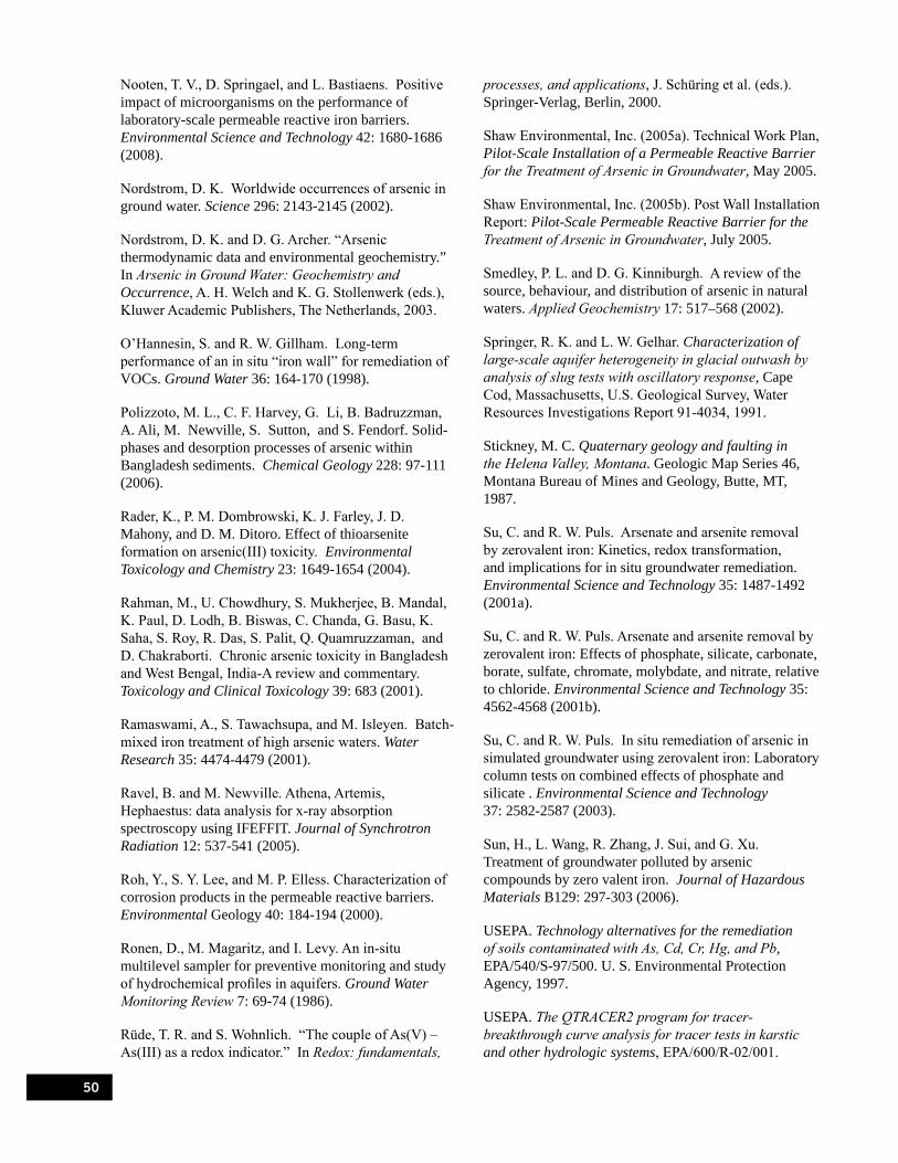
Nooten, T. V., D. Springael, and L. Bastiaens. Positive impact of microorganisms on the performance of laboratory-scale permeable reactive iron barriers. Environmental Science and Technology 42: 1680-1686 (2008).

Nordstrom, D. K. Worldwide occurrences of arsenic in ground water. Science 296: 2143-2145 (2002).

Nordstrom, D. K. and D. G. Archer. “Arsenic thermodynamic data and environmental geochemistry.” In Arsenic in Ground Water: Geochemistry and Occurrence, A. H. Welch and K. G. Stollenwerk (eds.), Kluwer Academic Publishers, The Netherlands, 2003.

O’Hannesin, S. and R. W. Gillham. Long-term performance of an in situ “iron wall” for remediation of VOCs. Ground Water 36: 164-170 (1998).

Polizzoto, M. L., C. F. Harvey, G. Li, B. Badruzzman, A. Ali, M. Newville, S. Sutton, and S. Fendorf. Solid-phases and desorption processes of arsenic within Bangladesh sediments. Chemical Geology 228: 97-111 (2006).

Rader, K., P. M. Dombrowski, K. J. Farley, J. D. Mahony, and D. M. Ditoro. Effect of thioarsenite formation on arsenic(III) toxicity. Environmental Toxicology and Chemistry 23: 1649-1654 (2004).

Rahman, M., U. Chowdhury, S. Mukherjee, B. Mandal, K. Paul, D. Lodh, B. Biswas, C. Chanda, G. Basu, K. Saha, S. Roy, R. Das, S. Palit, Q. Quamruzzaman, and D. Chakraborti. Chronic arsenic toxicity in Bangladesh and West Bengal, India-A review and commentary. Toxicology and Clinical Toxicology 39: 683 (2001).

Ramaswami, A., S. Tawachsupa, and M. Isleyen. Batch-mixed iron treatment of high arsenic waters. Water Research 35: 4474-4479 (2001).

Ravel, B. and M. Newville. Athena, Artemis, Hephaestus: data analysis for x-ray absorption spectroscopy using IFEFFIT. Journal of Synchrotron Radiation 12: 537-541 (2005).

Roh, Y., S. Y. Lee, and M. P. Elless. Characterization of corrosion products in the permeable reactive barriers. Environmental Geology 40: 184-194 (2000).

Ronen, D., M. Magaritz, and I. Levy. An in-situ multilevel sampler for preventive monitoring and study of hydrochemical profiles in aquifers. Ground Water Monitoring Review 7: 69-74 (1986).

Rüde, T. R. and S. Wohnlich. “The couple of As(V) – As(III) as a redox indicator.” In Redox: fundamentals,

processes, and applications, J. Schüring et al. (eds.). Springer-Verlag, Berlin, 2000.

Shaw Environmental, Inc. (2005a). Technical Work Plan, Pilot-Scale Installation of a Permeable Reactive Barrier for the Treatment of Arsenic in Groundwater, May 2005.

Shaw Environmental, Inc. (2005b). Post Wall Installation Report: Pilot-Scale Permeable Reactive Barrier for the Treatment of Arsenic in Groundwater, July 2005.

Smedley, P. L. and D. G. Kinniburgh. A review of the source, behaviour, and distribution of arsenic in natural waters. Applied Geochemistry 17: 517–568 (2002).

Springer, R. K. and L. W. Gelhar. Characterization of large-scale aquifer heterogeneity in glacial outwash by analysis of slug tests with oscillatory response, Cape Cod, Massachusetts, U.S. Geological Survey, Water Resources Investigations Report 91-4034, 1991.

Stickney, M. C. Quaternary geology and faulting in the Helena Valley, Montana. Geologic Map Series 46, Montana Bureau of Mines and Geology, Butte, MT, 1987.

Su, C. and R. W. Puls. Arsenate and arsenite removal by zerovalent iron: Kinetics, redox transformation, and implications for in situ groundwater remediation. Environmental Science and Technology 35: 1487-1492 (2001a).

Su, C. and R. W. Puls. Arsenate and arsenite removal by zerovalent iron: Effects of phosphate, silicate, carbonate, borate, sulfate, chromate, molybdate, and nitrate, relative to chloride. Environmental Science and Technology 35: 4562-4568 (2001b).

Su, C. and R. W. Puls. In situ remediation of arsenic in simulated groundwater using zerovalent iron: Laboratory column tests on combined effects of phosphate and silicate . Environmental Science and Technology 37: 2582-2587 (2003).

Sun, H., L. Wang, R. Zhang, J. Sui, and G. Xu. Treatment of groundwater polluted by arsenic compounds by zero valent iron. Journal of Hazardous Materials B129: 297-303 (2006).

USEPA. Technology alternatives for the remediation of soils contaminated with As, Cd, Cr, Hg, and Pb, EPA/540/S-97/500. U. S. Environmental Protection Agency, 1997.

USEPA. The QTRACER2 program for tracer-breakthrough curve analysis for tracer tests in karstic and other hydrologic systems, EPA/600/R-02/001.

50

Washington, D. C.: U. S. Environmental Protection Agency, 2002.

USEPA. Capstone report on the application, monitoring, and performance of permeable reactive barriers for ground-water remediation; Volume 1, Performance evaluations at two sites, EPA/600/R-03/045a. Cincinnati, OH: USEPA National Risk Management Research Laboratory, 2003a.

USEPA. Capstone report on the application, monitoring, and performance of permeable reactive barriers for ground-water remediation; Volume 2, Soiling sampling and ground water sampling, EPA/600/ R-03/045b. Cincinnati, OH: USEPA National Risk Management Research Laboratory, 2003b.

USEPA. Monitored Natural Attenuation of Inorganic Contaminants in Ground Water: Volume 2, Assessment for Non-radionuclides Including Arsenic, Cadmium, Chromium, Copper, Lead, Nickel, Nitrate, Perchlorate, and Selenium, EPA Report, EPA/600/R07/140, 2007.

Vlassopoulos, D., N. Rivera, P. A. O’Day, M. T. Rafferty, and C. B. Andrews. “Arsenic removal by zero-valent iron: a field study of rates, mechanisms, and long term performance.” In Advances in Arsenic Research: Integration of Experimental and Observational Studies and Implications for Migration, P.A. O’Day et al. (eds.). American Chemical Society Symposium Series 915, Ch. 25, 2005.

Webster, J. G. The solubility of As2S3 and speciation of As in dilute and sulphide-bearing fluids at 25 and 90 °C. Geochimica et Cosmochimica Acta 54: 1009-1017 (1990).

Welch, A. H., M. S. Lico, and J. L. Hughes. Arsenic in ground water of the western United States. Ground Water 26: 333-347 (1988).

Welch, A. H., D. B. Westjohn, D. R. Helsel, and R. B. Wanty. Arsenic in ground water of the United States: occurrence and geochemistry. Ground Water 38: 589-604 (2000).

Wilkin, R. T., D. Wallschläger, and R. G. Ford. Speciation of arsenic in sulfidic waters. Geochemical Transactions 4: 1-7 (2003).

Wilkin, R. T., R. W. Puls, and G. W. Sewell. Long-term performance of Permeable Reactive Barriers using zero-valent iron: geochemical and microbiological effects. Ground Water 41: 493-503 (2003).

Wilkin, R. T., C. Su, R. G. Ford, and C. J. Paul. Chromium removal processes during groundwater remediation by a zerovalent iron permeable reactive barrier. Environmental Science and Technology 39: 4599-4605 (2005).

Wilkin, R. T. and K. J. Bischoff. Coulometric determination of total sulfur and reduced inorganic sulfur fractions in environmental samples. Talanta 70: 766-773 (2006).

Wolthers, M., L. Charlet, C. H. van der Weijden, P. R. van der Linde, and D. Rickard. Arsenic mobility in the ambient sulfidic environment: sorption of arsenic(V) and arsenic(III) onto disordered mackinawite. Geochimica et Cosmochimica Acta 69: 3483-3492 (2005).

Young, S. C., H. E. Julian, H. S. Pearson, F. J. Molz, and G. K. Boman. Application of the electromagnetic borehole flowmeter, EPA/600/R-98/058. Ada, OK: U.S. Environmental Protection Agency, 1998.

Yuan, C. and T.-S. Chiang, The mechanisms of arsenic removal from soil by electrokinetic process coupled with iron permeable reaction barrier. Chemosphere 67: 1533­1542 (2007).

51

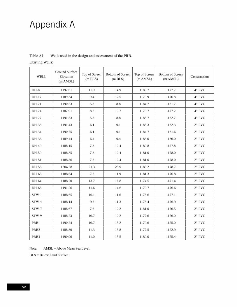
Appendix A

Table A1. Wells used in the design and assessment of the PRB.

Existing Wells:

WELL Ground Surface

Elevation (m AMSL)

Top of Screen (m BLS)

Bottom of Screen (m BLS)

Top of Screen (m AMSL)

Bottom of Screen (m AMSL)

Construction

DH-8 1192.61 11.9 14.9 1180.7 1177.7 4” PVC

DH-17 1189.34 9.4 12.5 1179.9 1176.8 4” PVC

DH-21 1190.53 5.8 8.8 1184.7 1181.7 4” PVC

DH-24 1187.91 8.2 10.7 1179.7 1177.2 4” PVC

DH-27 1191.53 5.8 8.8 1185.7 1182.7 4” PVC

DH-33 1191.43 6.1 9.1 1185.3 1182.3 2” PVC

DH-34 1190.75 6.1 9.1 1184.7 1181.6 2” PVC

DH-36 1189.44 6.4 9.4 1183.0 1180.0 2” PVC

DH-49 1188.15 7.3 10.4 1180.8 1177.8 2” PVC

DH-50 1188.35 7.3 10.4 1181.0 1178.0 2” PVC

DH-51 1188.36 7.3 10.4 1181.0 1178.0 2” PVC

DH-56 1204.58 21.3 25.9 1183.2 1178.7 2” PVC

DH-63 1188.64 7.3 11.9 1181.3 1176.8 2” PVC

DH-64 1188.20 13.7 16.8 1174.5 1171.4 2” PVC

DH-66 1191.26 11.6 14.6 1179.7 1176.6 2” PVC

STW-1 1188.65 10.1 11.6 1178.6 1177.1 2” PVC

STW-4 1188.14 9.8 11.3 1178.4 1176.9 2” PVC

STW-7 1188.67 7.6 12.2 1181.0 1176.5 2” PVC

STW-9 1188.23 10.7 12.2 1177.6 1176.0 2” PVC

PRB1 1190.24 10.7 15.2 1179.6 1175.0 2” PVC

PRB2 1188.80 11.3 15.8 1177.5 1172.9 2” PVC

PRB3 1190.96 11.0 15.5 1180.0 1175.4 2” PVC

Note: AMSL = Above Mean Sea Level.

BLS = Below Land Surface.

52

Wells Installed by USEPA:

WELL Ground Surface

Elevation (m AMSL)

Top of Screen

(m BLS)

Bottom of Screen (m BLS)

Top of Screen

(m AMSL)

Bottom of Screen

(m AMSL) Construction

EPA01 1189.72 10.1 14.6 1179.7 1175.1 2” PVC EPA02 1189.59 10.1 14.6 1179.5 1175.0 4” PVC EPA03 1189.35 10.1 14.6 1179.3 1174.7 2” PVC EPA04 1189.41 10.1 14.6 1179.4 1174.8 2” PVC EPA05 1188.89 10.1 14.6 1178.8 1174.3 2” PVC EPA06 1189.45 10.1 14.6 1179.4 1174.8 2” PVC EPA07 1188.99 10.1 14.6 1178.9 1174.4 2” PVC EPA08 1189.63 10.1 14.6 1179.6 1175.0 2” PVC EPA09 1189.60 10.1 14.6 1179.5 1175.0 2” PVC EPA10 1189.57 9.1 14.3 1180.4 1175.2 2” PVC PBTW-1 1189.29 9.4 13.7 1179.8 1175.6 2” PVC PBTW-2 1189.01 9.8 16.5 1179.3 1172.6 2” PVC S01 1189.57 13.0 13.7 1176.6 1175.9 1” PVC S02 1189.57 9.9 10.7 1179.7 1178.9 1” PVC S03 1189.58 13.0 13.7 1176.6 1175.9 1” PVC S04 1189.57 9.9 10.7 1179.7 1178.9 1” PVC S05 1189.59 11.4 12.2 1178.2 1177.4 1” PVC S06 1189.57 12.2 13.0 1177.4 1176.6 1” PVC S07 1189.61 12.2 13.0 1177.4 1176.7 1” PVC S08 1189.61 11.4 12.2 1178.2 1177.4 1” PVC T1A 1189.70 9.6 11.9 1180.1 1177.8 2” PVC T1B 1189.72 9.4 11.6 1180.4 1178.1 2” PVC T1C 1189.72 9.4 11.7 1180.3 1178.0 2” PVC T2A 1189.58 9.2 13.8 1180.4 1175.8 2” PVC T2B 1189.57 8.8 13.4 1180.8 1176.2 2” PVC T2C 1189.59 8.8 13.4 1180.8 1176.2 2” PVC T3A 1189.56 8.6 13.2 1181.0 1176.4 2” PVC T3B 1189.55 9.3 13.8 1180.3 1175.7 2” PVC T3C 1189.56 8.7 13.2 1180.9 1176.3 2” PVC TR1 1189.61 10.4 13.4 1179.2 1176.2 2” PVC TR2 1189.56 9.9 10.7 1179.7 1178.9 1” PVC TR3 1189.58 11.4 12.2 1178.1 1177.4 1” PVC TR4-1 1189.57 10.0 10.6 1179.6 1179.0 3 channel CMT TR4-2 1189.57 11.5 12.1 1178.1 1177.5 3 channel CMT TR4-3 1189.57 13.0 13.6 1176.6 1176.0 3 channel CMT TR5-1 1189.57 10.0 10.6 1179.6 1178.9 3 channel CMT TR5-2 1189.57 11.5 12.1 1178.0 1177.4 3 channel CMT TR5-3 1189.57 13.1 13.7 1176.5 1175.9 3 channel CMT TR6-1 1189.57 10.0 10.6 1179.6 1179.0 3 channel CMT TR6-2 1189.57 11.5 12.1 1178.1 1177.5 3 channel CMT TR6-3 1189.57 13.0 13.6 1176.6 1176.0 3 channel CMT TR7 1189.59 11.4 12.2 1178.2 1177.4 1” PVC TR8 1189.60 11.4 12.2 1178.2 1177.4 1” PVC TR9 1189.60 9.9 10.7 1179.7 1178.9 1” PVC TR10 1189.61 11.4 12.2 1178.2 1177.4 1” PVC TR11-1 1189.60 10.0 10.6 1179.6 1179.0 3 channel CMT TR11-2 1189.60 11.5 12.1 1178.1 1177.5 3 channel CMT TR11-3 1189.60 13.0 13.6 1176.6 1176.0 3 channel CMT TR12-1 1189.60 10.0 10.6 1179.6 1179.0 3 channel CMT TR12-2 1189.60 11.6 12.2 1178.1 1177.4 3 channel CMT TR12-3 1189.60 13.1 13.7 1176.5 1175.9 3 channel CMT

53

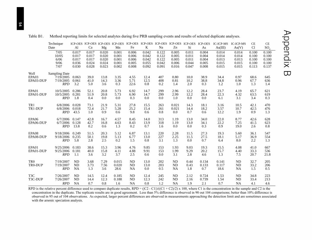
TechniqueDate

ICP-OES ICP-OES ICP-OES ICP-OESAl Ca Mg Mn

ICP-OESFe

ICP-OESK

ICP-OESNa

ICP-OESZn

ICP-OES Si

ICP-OESAs

IC-ICP-MSAs(III)

IC-ICP-MSAs(V)

CECl

CESO4

7/05 10/05 6/06 9/06 7/07

0.017 0.017 0.020 0.001 0.017 0.017 0.020 0.001 0.017 0.017 0.020 0.001 0.036 0.024 0.024 0.001 0.030 0.028 0.023 0.002

0.006 0.006 0.006 0.005 0.008

0.042 0.042 0.042 0.055 0.092

0.122 0.122 0.122 0.042 0.091

0.005 0.005 0.005 0.006 0.016

0.011 0.011 0.011 0.044 0.047

0.004 0.004 0.004 0.005 0.008

0.014 0.014 0.013 0.015 0.015

0.014 0.014 0.013 0.015 0.015

0.100 0.100 0.100 0.100 0.113

0.100 0.100 0.100 0.100 0.137

Well EPA03 EPA03-DUP

Sampling Date7/19/2005 7/19/2005

RPD

0.063 39.0 13.8 3.35 0.061 41.0 14.3 3.36 3.2 5.0 3.6 0.3

4.55 5.71 22.6

12.4 12.5 0.8

407 408 0.2

0.80 0.81 1.4

10.0 10.2 2.0

38.9 38.8 0.3

34.4 34.8 1.2

0.97 0.96 1.0

68.6 67.7 1.3

645 636 1.4

EPA01 EPA01-DUP

10/5/2005 10/5/2005

RPD

0.286 52.1 20.8 5.73 0.281 51.9 20.8 5.73 1.8 0.4 0.0 0.0

6.92 6.90 0.3

14.7 14.7 0.0

299 299 0.0

2.96 2.99 1.0

12.2 12.2 0.0

28.4 28.4 0.0

23.7 22.3 6.1

4.19 4.32 3.1

65.7 63.5 3.4

621 619 0.3

TR1 TR1-DUP

6/8/2006 6/8/2006

RPD

0.028 73.1 21.9 5.31 0.018 72.4 21.7 5.28 43.5 1.0 0.9 0.6

27.8 25.2 9.8

15.5 15.4 0.6

263 261 0.8

0.021 0.021 0.0

14.3 14.4 0.7

18.1 18.2 0.6

3.16 3.57 12.2

10.5 10.7 1.9

42.1 42.5 0.9

470 476 1.3

EPA06 EPA06-DUP

6/7/2006 6/7/2006

RPD

0.147 42.8 16.7 4.57 0.128 42.7 16.8 4.63 13.8 0.2 0.6 1.3

8.45 8.43 0.2

14.0 13.9 0.7

313 318 1.6

1.19 1.19 0.0

13.0 13.0 0.0

34.0 34.1 0.3

22.0 22.2 0.9

8.77 7.25 19.0

42.6 41.5 2.6

628 623 0.8

EPA08 EPA08-DUP

9/18/2006 9/18/2006

RPD

0.249 51.5 20.3 5.12 0.235 50.1 19.8 5.13 5.8 2.8 2.5 0.2

6.87 6.77 1.5

13.1 13.0 0.8

220 227 3.1

2.28 2.25 1.3

11.5 11.5 0.0

27.3 27.5 0.7

19.3 18.1 6.4

5.60 5.17 8.0

36.1 36.9 2.2

547 554 1.3

EPA01 EPA01-DUP

9/25/2006 9/25/2006

RPD

0.183 38.6 15.3 3.96 0.181 40.0 15.8 4.11 1.1 3.6 3.2 3.7

4.76 4.88 2.5

9.85 9.91 0.6

153 153 0.0

1.93 1.99 3.1

9.03 9.29 2.8

19.3 20.2 4.6

15.5 15.7 1.3

4.08 4.40 7.5

41.0 33.3 20.7

667 536 21.8

TR0 TR0-DUP

7/19/2007 7/19/2007

RPD

ND 3.68 7.29 0.015 ND 3.73 7.56 0.020 NA 1.3 3.6 28.6

ND ND NA

13.0 13.0 0.0

202 203 0.5

ND ND NA

0.44 0.43 1.8

0.134 0.133 0.7

0.141 0.117 18.6

ND ND NA

32.7 33.2 1.5

205 206 0.5

T3C T3C-DUP

7/26/2007 7/26/2007

ND 14.5 12.4 0.185 ND 14.4 12.3 0.188

ND ND

12.4 12.3

245 242

ND ND

2.12 2.16

0.724 0.739

1.53 1.54

ND ND

34.8 33.4

223 213

RPD NA 0.7 0.8 1.6 NA 0.8 1.2 NA 1.9 2.1 0.7 NA 4.1 4.6

54

Table B1. Method reporting limits for selected analytes during five PRB sampling events and results of selected duplicate analyses.

RPD is the relative percent difference used to compare duplicate results, RPD = (|C2 - C1|)/((C1 + C2)/2) x 100, where C1 is the concentration in the sample and C2 is the concentration in the duplicate. The replicate results are in good agreement. Less than 5% difference is observed in 90 out 104 comparisons; better than 10% difference is observed in 95 out of 104 observations. As expected, larger percent differences are observed in measurements approaching the detection limit and are sometimes associated with the arsenic speciation analysis.

Appendix B

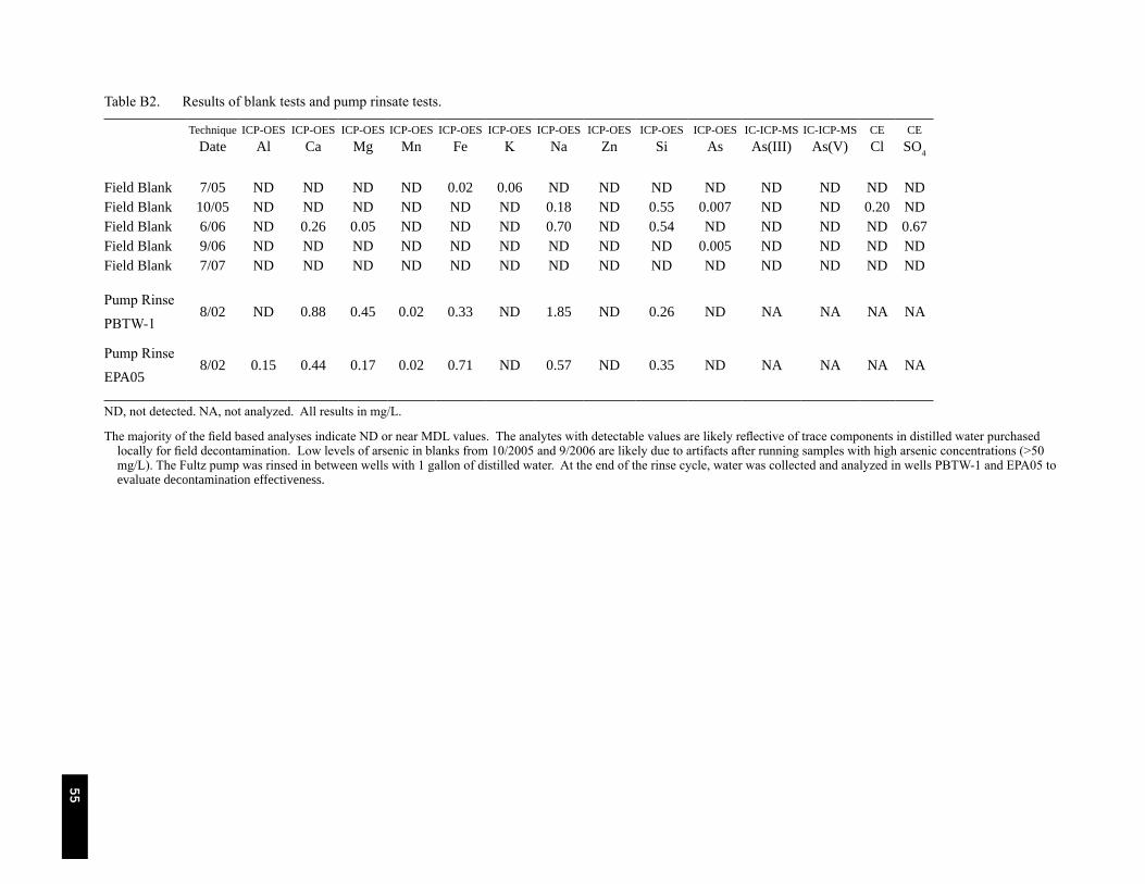
Technique ICP-OES ICP-OES ICP-OES ICP-OES ICP-OES ICP-OES ICP-OES ICP-OES ICP-OES ICP-OES IC-ICP-MS IC-ICP-MS CE CEDate Al Ca Mg Mn Fe K Na Zn Si As As(III) As(V) Cl SO4

Field Blank 7/05 ND ND ND ND 0.02 0.06 ND ND ND ND ND ND ND ND Field Blank 10/05 ND ND ND ND ND ND 0.18 ND 0.55 0.007 ND ND 0.20 ND Field Blank 6/06 ND 0.26 0.05 ND ND ND 0.70 ND 0.54 ND ND ND ND 0.67 Field Blank 9/06 ND ND ND ND ND ND ND ND ND 0.005 ND ND ND ND Field Blank 7/07 ND ND ND ND ND ND ND ND ND ND ND ND ND ND

Pump Rinse

PBTW-1 8/02 ND 0.88 0.45 0.02 0.33 ND 1.85 ND 0.26 ND NA NA NA NA

Pump Rinse

EPA05 8/02 0.15 0.44 0.17 0.02 0.71 ND 0.57 ND 0.35 ND NA NA NA NA

Table B2. Results of blank tests and pump rinsate tests.

ND, not detected. NA, not analyzed. All results in mg/L.

The majority of the field based analyses indicate ND or near MDL values. The analytes with detectable values are likely reflective of trace components in distilled water purchasedlocally for field decontamination. Low levels of arsenic in blanks from 10/2005 and 9/2006 are likely due to artifacts after running samples with high arsenic concentrations (>50mg/L). The Fultz pump was rinsed in between wells with 1 gallon of distilled water. At the end of the rinse cycle, water was collected and analyzed in wells PBTW-1 and EPA05 to evaluate decontamination effectiveness.

55

Appendix C

Table C1. Thermodynamic data for arsenic oxyanions.

MINTEQA21 WATEQ4f2 LLNL3 Nordstrom and Archer

(2003)

Raposo et al. (2004)

Zakaznova-Herzog et al.

(2006)

Reaction As(III) species

H3AsO3(aq) = H2AsO3 - + H+ -9.38 -9.36 -9.23 -9.15 -9.25

H2AsO3 - = HAsO3

2- + H+ -14.35 -14.70 -11.01 -14.70

HAsO3 2­ = AsO3

3- + H+ ND -15.70 ND -15.70

As(V) species

H3AsO4(aq) = H2AsO4 - + H+ -2.24 -2.25 -2.25 -2.30 -2.25

H2AsO4 - = HAsO4

2- + H+ -7.01 -7.18 -6.75 -7.16 -7.06

HAsO4 2- = AsO4

3- + H+ -11.94 -11.79 -11.90 -11.65 -11.58

Redox H3AsO4(aq) + H2(g) = H3AsO3(aq) + H2O(l) 22.96 23.40 22.56 19.35

1 Allison, J. D., Brown, D. S., and Nova-Gradac, K. J. (1990). MINTEQA2/PRODEFA2, A geochemical assessment model for environmental systems. USEPA, EPA/600/3-91/021.

2 Ball, J. W. and Nordstrom, D. K. (1991). User’s manual for WATEQ4F, with revised thermodynamic data base. USGS Open File Report 91-183.

3 Dataset from Lawrence Livermore National Laboratory, thermo.dat. Wolery, T. J. (1992). EQ3/6, a software package for geochemical modeling of aqueous systems, package overview and installation guide (version 7.0). Technical Report UCRL-MA-110662, Part 1, Lawrence Livermore National Laboratory.

Nordstrom, D. K. and Archer, D. G. (2003). Arsenic thermodynamic data and environmental geochemistry. In Arsenic in Ground Water: Geochemistry and Occurrence, Welch, A. H. and Stollenwerk, K. G., eds. Kluwer Academic Publishers, The Netherlands.

Raposo, J. C., Zuloaga, O., Olazabal, M. A., and Madariaga, J. M. (2004). Study of the precipitation equilibria of arsenate anion with calcium and magnesium in sodium perchlorate at 25°C. Applied Geochemistry, v. 19, p. 855-862.

Zakaznova-Herzog, V. P., Seward, T. M., and Suleimenov, O. M. (2006). Arsenous acid ionization in aqueous solutions from 25 to 300 °C. Geochimica et Cosmochimica Acta, v. 70, p. 1928-1938.

56

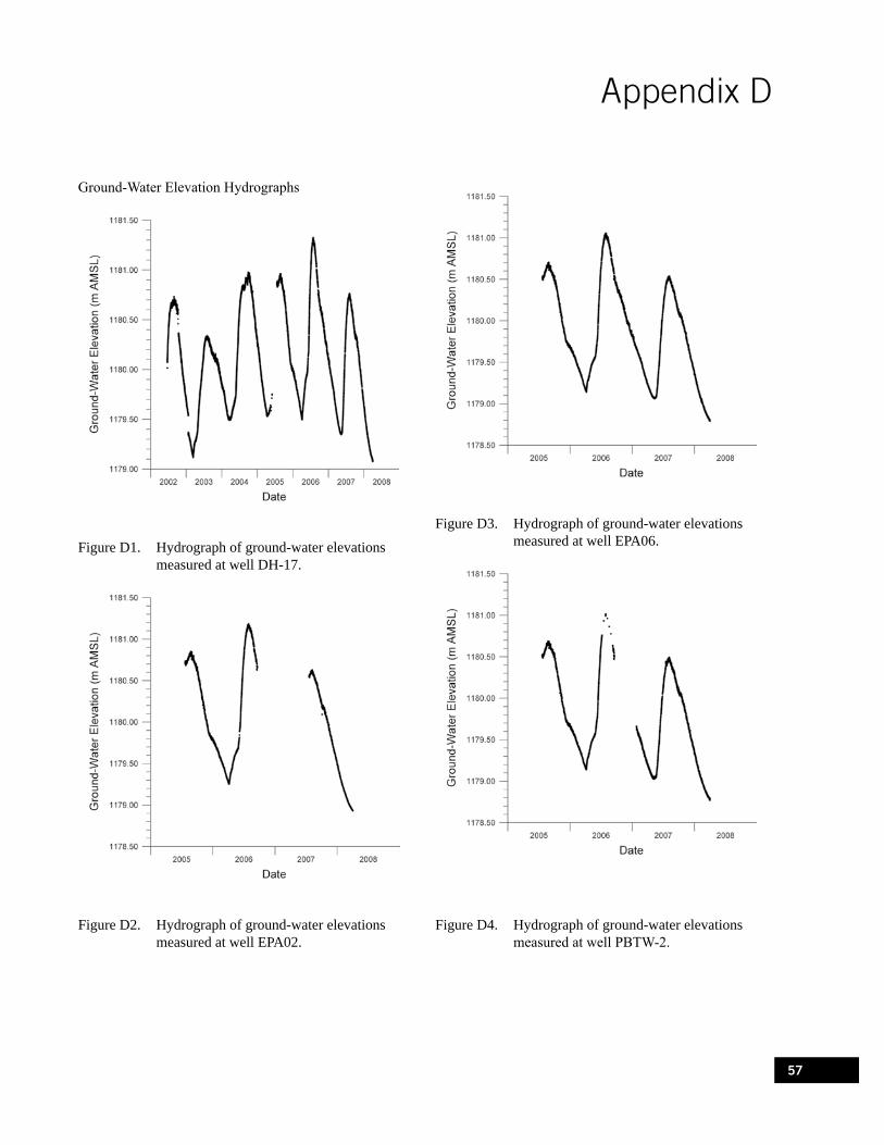
Figure D1. Hydrograph of ground-water elevations measured at well DH-17.

Figure D2. Hydrograph of ground-water elevations measured at well EPA02.

Figure D3. Hydrograph of ground-water elevations measured at well EPA06.

Figure D4. Hydrograph of ground-water elevations measured at well PBTW-2.

Appendix D

Ground-Water Elevation Hydrographs

57

Figure D5. Hydrograph of ground-water elevations measured at well TR8.

58

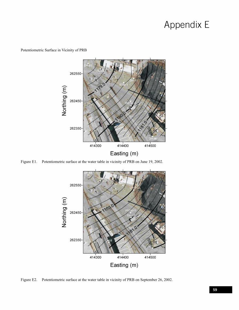
Appendix E

Potentiometric Surface in Vicinity of PRB

Figure E1. Potentiometric surface at the water table in vicinity of PRB on June 19, 2002.

Figure E2. Potentiometric surface at the water table in vicinity of PRB on September 26, 2002.

59

Figure E3. Potentiometric surface at the water table in vicinity of PRB on August 14, 2003.

60

Figure E4. Potentiometric surface at the water table in vicinity of PRB on May 31, 2005.

Figure E5. Potentiometric surface at the water table in vicinity of PRB on July 20, 2005.

Figure E6. Potentiometric surface at the water table in vicinity of PRB on October 6, 2005.

61

Figure E7. Potentiometric surface at the water table in vicinity of PRB on June 6, 2006.

62

Figure E8. Potentiometric surface at the water table in vicinity of PRB on September 18, 2006.

Figure E9. Potentiometric surface at the water table in vicinity of PRB on January 24, 2007.

Figure E10. Potentiometric surface at the water table in vicinity of PRB on July 18/19, 2007.

63

Figure E11. Potentiometric surface at the water table in vicinity of PRB on October 1, 2007.

64

Figure E12. Potentiometric surface at the water table in vicinity of PRB on April 1, 2008.

Figure E13. Potentiometric surface at the water table in vicinity of PRB on June 24, 2008.

65

Office of Research and Development (8101R) Washington, DC 20460

Official Business Penalty for Private Use $300

PRESORTED STANDARD POSTAGE & FEES PAID

EPA PERMIT NO. G-35