
FICHA CATALOGRÁFICA ELABORADA PELArocha/pub/papers/2009-phd-thesis-ander… · FICHA...
199
Transcript of FICHA CATALOGRÁFICA ELABORADA PELArocha/pub/papers/2009-phd-thesis-ander… · FICHA...


FICHA CATALOGRÁFICA ELABORADA PELA BIBLIOTECA DO IMECC DA UNICAMP
Bibliotecária: Crisllene Queiroz Custódio – CRB8 / 7966
Rocha, Anderson de Rezende
R582c Classificadores e aprendizado em processamento de imagens e visão
computacional / Anderson de Rezende Rocha -- Campinas, [S.P. : s.n.], 2009.
Orientador : Siome Klein Goldenstein
Tese (Doutorado) - Universidade Estadual de Campinas, Instituto de
Computação.
1. Aprendizado de máquina - Técnicas. 2. Análise forense de imagens.
3. Esteganálise. 4. Fusão de características. 5. Fusão de classificadores.
6. Classificação multi-classe. 7. Categorização de imagens. I. Goldenstein,
Siome Klein. II. Universidade Estadual de Campinas. Instituto de Computação.
III. Título
(cqc/imecc)
Título em inglês: Classifiers and machine learning techniques for image processing and computer vision
Palavras-chave em inglês (Keywords): 1. Machine learning - Techniques. 2. Digital forensics. 3. Steganalysis. 4. Feature fusion. 5. Classifier fusion. 6. Multi-class classification. 7. Image categorization.
Área de concentração: Visão Computacional
Titulação: Doutor em Ciência da Computação
Banca examinadora: Prof. Dr. Siome Klein Goldenstein (IC-UNICAMP)Prof. Dr. Fábio Gagliardi Cozman (Mecatrônica-Poli/USP)Prof. Dr. Luciano da Fontoura Costa (IF-USP/São Carlos)Prof. Dr. Ricardo Dahab (IC-UNICAMP)Prof. Dr. Roberto de Alencar Lotufo (FEEC-UNICAMP)
Data da defesa: 03/03/2009
Programa de Pós-Graduação: Doutorado em Ciência da Computação


Instituto de Computacao
Universidade Estadual de Campinas
Classificadores e Aprendizado em
Processamento de Imagens e Visao Computacional
Anderson de Rezende Rocha1
3 de marco de 2009
Banca Examinadora:
• Prof. Dr. Siome Klein Goldenstein (Orientador)
• Prof. Dr. Fabio Gagliardi Cozman
Depto. de Mecatronica e Sistemas Mecanicos (Poli-USP)
• Prof. Dr. Luciano da Fontoura Costa
Instituto de Fısica de Sao Carlos (USP)
• Prof. Dr. Ricardo Dahab
Instituto de Computacao (Unicamp)
• Prof. Dr. Roberto de Alencar Lotufo
Faculdade de Engenharia Eletrica e de Computacao (Unicamp)
1Financiado pela Fundacao de Amparo a Pesquisa do Estado de Sao Paulo (FAPESP), processonumero 05/58103-3.
v


Resumo
Neste trabalho de doutorado, propomos a utilizacao de classificadores e tecnicas de aprendizado
de maquina para extrair informacoes relevantes de um conjunto de dados (e.g., imagens) para
solucao de alguns problemas em Processamento de Imagens e Visao Computacional.
Os problemas de nosso interesse sao: categorizacao de imagens em duas ou mais classes,
deteccao de mensagens escondidas, distincao entre imagens digitalmente adulteradas e imagens
naturais, autenticacao, multi-classificacao, entre outros.
Inicialmente, apresentamos uma revisao comparativa e crıtica do estado da arte em analise
forense de imagens e deteccao de mensagens escondidas em imagens. Nosso objetivo e mostrar
as potencialidades das tecnicas existentes e, mais importante, apontar suas limitacoes. Com
esse estudo, mostramos que boa parte dos problemas nessa area apontam para dois pontos em
comum: a selecao de caracterısticas e as tecnicas de aprendizado a serem utilizadas. Nesse
estudo, tambem discutimos questoes legais associadas a analise forense de imagens como, por
exemplo, o uso de fotografias digitais por criminosos.
Em seguida, introduzimos uma tecnica para analise forense de imagens testada no contexto
de deteccao de mensagens escondidas e de classificacao geral de imagens em categorias como
indoors, outdoors, geradas em computador e obras de arte.
Ao estudarmos esse problema de multi-classificacao, surgem algumas questoes: como re-
solver um problema multi-classe de modo a poder combinar, por exemplo, caracterısticas de
classificacao de imagens baseadas em cor, textura, forma e silhueta, sem nos preocuparmos
demasiadamente em como normalizar o vetor-comum de caracterısticas gerado? Como utili-
zar diversos classificadores diferentes, cada um, especializado e melhor configurado para um
conjunto de caracterısticas ou classes em confusao? Nesse sentido, apresentamos, uma tecnica
para fusao de classificadores e caracterısticas no cenario multi-classe atraves da combinacao de
classificadores binarios. Nos validamos nossa abordagem numa aplicacao real para classificacao
automatica de frutas e legumes.
Finalmente, nos deparamos com mais um problema interessante: como tornar a utilizacao
de poderosos classificadores binarios no contexto multi-classe mais eficiente e eficaz? Assim,
introduzimos uma tecnica para combinacao de classificadores binarios (chamados classificadores
base) para a resolucao de problemas no contexto geral de multi-classificacao.
vii


Abstract
In this work, we propose the use of classifiers and machine learning techniques to extract useful
information from data sets (e.g., images) to solve important problems in Image Processing and
Computer Vision.
We are particularly interested in: two and multi-class image categorization, hidden mes-
sages detection, discrimination among natural and forged images, authentication, and multi-
classification.
To start with, we present a comparative survey of the state-of-the-art in digital image foren-
sics as well as hidden messages detection. Our objective is to show the importance of the existing
solutions and discuss their limitations. In this study, we show that most of these techniques
strive to solve two common problems in Machine Learning: the feature selection and the classi-
fication techniques to be used. Furthermore, we discuss the legal and ethical aspects of image
forensics analysis, such as, the use of digital images by criminals.
We introduce a technique for image forensics analysis in the context of hidden messages
detection and image classification in categories such as indoors, outdoors, computer generated,
and art works.
From this multi-class classification, we found some important questions: how to solve a
multi-class problem in order to combine, for instance, several different features such as color,
texture, shape, and silhouette without worrying about the pre-processing and normalization of
the combined feature vector? How to take advantage of different classifiers, each one custom
tailored to a specific set of classes in confusion? To cope with most of these problems, we present
a feature and classifier fusion technique based on combinations of binary classifiers. We validate
our solution with a real application for automatic produce classification.
Finally, we address another interesting problem: how to combine powerful binary classifiers
in the multi-class scenario more effectively? How to boost their efficiency? In this context,
we present a solution that boosts the efficiency and effectiveness of multi-class from binary
techniques.
ix

Agradecimentos
Toda caminhada apresenta desafios e dificuldades. O que seria de nos se, nesses momentos, nao
pudessemos contar com nossos amigos e colegas?
Estou realizando o sonho de ser doutor. Quando saı de minha pequena cidade aos 10 anos de
idade para estudar esse nem parecia ser um sonho alcancavel. No entanto, os dia se passaram, e
aqui estou hoje amadurecido pelo tempo e agradecendo a ajuda das muitas pessoas com quem
cruzei durante a vida. Gostaria de citar algumas delas, mesmo correndo o risco de deixar algumas
de fora. A estas, desculpo-me antecipadamente.
Primeiramente, agradeco as duas pessoas mais importantes de minha vida: minha mae
Lucılia e minha esposa Aninha. Voces sao minha inspiracao.
Gostaria de estender os agradecimentos ao meu pai Antonio Carlos que, mesmo em sua
simplicidade, entende as dificuldades de uma caminhada como essa. As minhas irmas Aline
e Ana Carla por sempre acreditarem em mim. Agradeco tambem a Regina Celia pelo apoio
constante.
Quero agradecer ao meu orientador Siome Goldenstein. Suas dicas foram muito importantes
para o meu crescimento nao so como estudante mas tambem como pesquisador e cidadao. Com
voce, Siome, aprendi muita coisa, principalmente a fazer as perguntas corretas e a ser crıtico.
Estendo meus agradecimentos aos professores da Unicamp com quem tive a oportunidade de
ser aluno como: Alexandre Falcao, Anamaria Gomide, Jacques Wainer, Neucimar Leite, Ricardo
Anido, Ricardo Panain, Ricardo Torres e Yuzo Iano.
Agradeco aos meus muitos colegas de laboratorio por discussoes importantes. Em especial
agradeco aos diversos colegas com quem tive a oportunidade de ser um colaborador de pesquisa.
Agradeco tambem aos meus colegas de apartamento Luıs Meira e Wilson Pavon. Obrigado a
todos pela amizade.
Nao posso esquecer de mencionar o agradecimento a Unicamp. Esta e uma universidade que
apoia o estudante em todos os momentos. E bom saber que o Brasil possui lugares como esse.
Ajuda-nos a crer que o paıs tem jeito, basta acreditarmos. Finalmente, agradeco a FAPESP
pelo apoio financeiro sem o qual eu nao poderia me dedicar integralmente a essa pesquisa.
xi


Epıgrafe
Every day I remind myself that my inner and
outer life are based on the labors of other men,
living and dead, and that I must exert myself
in order to give in the same measure as I have
received and am still receiving.
(Albert Einstein)
xiii


Dedicatoria
Dedico este trabalho a minha mae Lucılia.
Mae, os pobres tambem podem. Dedico tambem
a minha esposa Aninha, por ser minha “prin-
cipeza”. Aninha, voce e um presente para mim.
Isso e para voces.
xv


Sumario
Resumo vii
Abstract ix
Agradecimentos xi
1 Introducao 1
1.1 Deteccao de adulteracoes em imagens digitais . . . . . . . . . . . . . . . . . . . . 3
1.2 Esteganalise e categorizacao de imagens . . . . . . . . . . . . . . . . . . . . . . . 5
1.2.1 Deteccao de mensagens escondidas . . . . . . . . . . . . . . . . . . . . . . 5
1.2.2 Categorizacao de imagens – Cenario de duas classes . . . . . . . . . . . . 5
1.2.3 Categorizacao de imagens – Cenario multi-classe . . . . . . . . . . . . . . 5
1.2.4 Randomizacao Progressiva (PR) . . . . . . . . . . . . . . . . . . . . . . . 6
1.2.5 Resultados obtidos . . . . . . . . . . . . . . . . . . . . . . . . . . . . . . . 9
1.3 Fusao multi-classe de caracterısticas e classificadores . . . . . . . . . . . . . . . . 9
1.3.1 Solucao proposta . . . . . . . . . . . . . . . . . . . . . . . . . . . . . . . . 10
1.3.2 Resultados obtidos . . . . . . . . . . . . . . . . . . . . . . . . . . . . . . . 13
1.4 Multi-classe a partir de classificadores binarios . . . . . . . . . . . . . . . . . . . 13
1.4.1 Affine-Bayes . . . . . . . . . . . . . . . . . . . . . . . . . . . . . . . . . . . 13
1.4.2 Resultados obtidos . . . . . . . . . . . . . . . . . . . . . . . . . . . . . . . 15
2 Current Trends and Challenges in Digital Image Forensics 19
2.1 Introduction . . . . . . . . . . . . . . . . . . . . . . . . . . . . . . . . . . . . . . . 19
2.2 Vision techniques for the Unseen . . . . . . . . . . . . . . . . . . . . . . . . . . . 23
2.2.1 Image manipulation techniques . . . . . . . . . . . . . . . . . . . . . . . . 23
2.2.2 Important questions . . . . . . . . . . . . . . . . . . . . . . . . . . . . . . 24
2.2.3 Source Camera Identification . . . . . . . . . . . . . . . . . . . . . . . . . 25
2.2.4 Image and video tampering detection . . . . . . . . . . . . . . . . . . . . 34
2.2.5 Image and video hidden content detection/recovery . . . . . . . . . . . . . 43
2.3 Conclusions . . . . . . . . . . . . . . . . . . . . . . . . . . . . . . . . . . . . . . . 54
2.4 Acknowledgments . . . . . . . . . . . . . . . . . . . . . . . . . . . . . . . . . . . . 55
xvii

3 Steganography and Steganalysis in Digital Multimedia: Hype or Hallelujah? 59
3.1 Introduction . . . . . . . . . . . . . . . . . . . . . . . . . . . . . . . . . . . . . . . 59
3.2 Terminology . . . . . . . . . . . . . . . . . . . . . . . . . . . . . . . . . . . . . . . 60
3.3 Historical remarks . . . . . . . . . . . . . . . . . . . . . . . . . . . . . . . . . . . 62
3.4 Social impacts . . . . . . . . . . . . . . . . . . . . . . . . . . . . . . . . . . . . . 63
3.5 Scientific and commercial applications . . . . . . . . . . . . . . . . . . . . . . . . 64
3.6 Steganography . . . . . . . . . . . . . . . . . . . . . . . . . . . . . . . . . . . . . 65
3.6.1 LSB insertion/modification . . . . . . . . . . . . . . . . . . . . . . . . . . 66
3.6.2 FFTs and DCTs . . . . . . . . . . . . . . . . . . . . . . . . . . . . . . . . 67
3.6.3 How to improve security . . . . . . . . . . . . . . . . . . . . . . . . . . . . 69
3.7 Steganalysis . . . . . . . . . . . . . . . . . . . . . . . . . . . . . . . . . . . . . . . 70
3.7.1 χ2 analysis . . . . . . . . . . . . . . . . . . . . . . . . . . . . . . . . . . . 71
3.7.2 RS analysis . . . . . . . . . . . . . . . . . . . . . . . . . . . . . . . . . . . 72
3.7.3 Gradient-energy flipping rate . . . . . . . . . . . . . . . . . . . . . . . . . 73
3.7.4 High-order statistical analysis . . . . . . . . . . . . . . . . . . . . . . . . . 74
3.7.5 Image quality metrics . . . . . . . . . . . . . . . . . . . . . . . . . . . . . 75
3.7.6 Progressive Randomization (PR) . . . . . . . . . . . . . . . . . . . . . . . 76
3.8 Freely available tools and software . . . . . . . . . . . . . . . . . . . . . . . . . . 79
3.9 Open research topics . . . . . . . . . . . . . . . . . . . . . . . . . . . . . . . . . . 80
3.10 Conclusions . . . . . . . . . . . . . . . . . . . . . . . . . . . . . . . . . . . . . . . 80
3.11 Acknowledgments . . . . . . . . . . . . . . . . . . . . . . . . . . . . . . . . . . . . 80
4 Progressive Randomization: Seeing the Unseen 83
4.1 Introduction . . . . . . . . . . . . . . . . . . . . . . . . . . . . . . . . . . . . . . . 83
4.2 Related work . . . . . . . . . . . . . . . . . . . . . . . . . . . . . . . . . . . . . . 85
4.2.1 Image Categorization . . . . . . . . . . . . . . . . . . . . . . . . . . . . . 85
4.2.2 Digital Steganalysis . . . . . . . . . . . . . . . . . . . . . . . . . . . . . . 86
4.3 Progressive Randomization approach (PR) . . . . . . . . . . . . . . . . . . . . . . 87
4.3.1 Pixel perturbation . . . . . . . . . . . . . . . . . . . . . . . . . . . . . . . 87
4.3.2 The randomization process . . . . . . . . . . . . . . . . . . . . . . . . . . 88
4.3.3 Feature region selection . . . . . . . . . . . . . . . . . . . . . . . . . . . . 88
4.3.4 Statistical descriptors . . . . . . . . . . . . . . . . . . . . . . . . . . . . . 89
4.3.5 Invariance . . . . . . . . . . . . . . . . . . . . . . . . . . . . . . . . . . . . 91
4.4 Experiments and results – Image Categorization . . . . . . . . . . . . . . . . . . 92
4.4.1 Experiment 1 . . . . . . . . . . . . . . . . . . . . . . . . . . . . . . . . . . 93
4.4.2 Experiment 2 . . . . . . . . . . . . . . . . . . . . . . . . . . . . . . . . . . 96
4.4.3 Experiment 3 . . . . . . . . . . . . . . . . . . . . . . . . . . . . . . . . . . 96
4.4.4 Experiment 4 . . . . . . . . . . . . . . . . . . . . . . . . . . . . . . . . . . 97
4.5 Experiments and results – Steganalysis . . . . . . . . . . . . . . . . . . . . . . . . 97
4.5.1 Overall results . . . . . . . . . . . . . . . . . . . . . . . . . . . . . . . . . 98
4.5.2 Class-based Steganalysis . . . . . . . . . . . . . . . . . . . . . . . . . . . . 99
xviii
4.5.3 Comparison . . . . . . . . . . . . . . . . . . . . . . . . . . . . . . . . . . . 100
4.6 Why does PR work? . . . . . . . . . . . . . . . . . . . . . . . . . . . . . . . . . . 102
4.7 Limitations . . . . . . . . . . . . . . . . . . . . . . . . . . . . . . . . . . . . . . . 104
4.8 Conclusions and remarks . . . . . . . . . . . . . . . . . . . . . . . . . . . . . . . . 105
5 Automatic Fruit and Vegetable Classification from Images 111
5.1 Introduction . . . . . . . . . . . . . . . . . . . . . . . . . . . . . . . . . . . . . . . 111
5.2 Literature review . . . . . . . . . . . . . . . . . . . . . . . . . . . . . . . . . . . . 113
5.3 Materials and methods . . . . . . . . . . . . . . . . . . . . . . . . . . . . . . . . . 114
5.3.1 Supermarket Produce data set . . . . . . . . . . . . . . . . . . . . . . . . 114
5.3.2 Image descriptors . . . . . . . . . . . . . . . . . . . . . . . . . . . . . . . . 117
5.3.3 Supervised learning . . . . . . . . . . . . . . . . . . . . . . . . . . . . . . 119
5.4 Background subtraction . . . . . . . . . . . . . . . . . . . . . . . . . . . . . . . . 123
5.5 Preliminary results . . . . . . . . . . . . . . . . . . . . . . . . . . . . . . . . . . . 125
5.6 Feature and classifier fusion . . . . . . . . . . . . . . . . . . . . . . . . . . . . . . 128
5.7 Fusion results . . . . . . . . . . . . . . . . . . . . . . . . . . . . . . . . . . . . . . 130
5.7.1 General fusion results . . . . . . . . . . . . . . . . . . . . . . . . . . . . . 131
5.7.2 Top two responses . . . . . . . . . . . . . . . . . . . . . . . . . . . . . . . 132
5.8 Conclusions and remarks . . . . . . . . . . . . . . . . . . . . . . . . . . . . . . . . 133
6 From Binary to Multi-class: A Bayesian Evolution 139
6.1 Introduction . . . . . . . . . . . . . . . . . . . . . . . . . . . . . . . . . . . . . . . 139
6.2 State-of-the-Art . . . . . . . . . . . . . . . . . . . . . . . . . . . . . . . . . . . . . 141
6.3 Affine-Bayes Multi-class . . . . . . . . . . . . . . . . . . . . . . . . . . . . . . . . 143
6.3.1 Affinity matrix A . . . . . . . . . . . . . . . . . . . . . . . . . . . . . . . . 145
6.3.2 Clustering . . . . . . . . . . . . . . . . . . . . . . . . . . . . . . . . . . . . 146
6.3.3 Shrinking . . . . . . . . . . . . . . . . . . . . . . . . . . . . . . . . . . . . 148
6.3.4 Augmenting . . . . . . . . . . . . . . . . . . . . . . . . . . . . . . . . . . . 148
6.4 Experiments and Results . . . . . . . . . . . . . . . . . . . . . . . . . . . . . . . . 151
6.4.1 Scenario 1 (10 to 26 classes) . . . . . . . . . . . . . . . . . . . . . . . . . . 152
6.4.2 Scenario 2 (95 to 1,000 classes) . . . . . . . . . . . . . . . . . . . . . . . . 154
6.5 Conclusions and Remarks . . . . . . . . . . . . . . . . . . . . . . . . . . . . . . . 158
7 Conclusoes 161
7.1 Deteccao de adulteracoes em imagens digitais . . . . . . . . . . . . . . . . . . . . 161
7.2 Randomizacao Progressiva . . . . . . . . . . . . . . . . . . . . . . . . . . . . . . . 162
7.3 Fusao multi-classe de caracterısticas e classificadores . . . . . . . . . . . . . . . . 163
7.4 Multi-classe a partir de classificadores binarios . . . . . . . . . . . . . . . . . . . 163
Bibliografia 165
xix


Capıtulo 1
Introducao
Em Processamento de Imagens e Visao Computacional, muitas vezes, a solucao de determinados
problemas pode exigir o correto entendimento do contexto da cena analisada ou mesmo das
inter-relacoes compartilhadas por cenas de um mesmo grupo semantico. No entanto, definir
precisamente as nuancas e caracterısticas que gostarıamos de selecionar nao e uma tarefa facil.
Nesse contexto, tecnicas de aprendizado de maquina e reconhecimento de padroes podem tornar-
se ferramentas valiosas.
A extracao de caracterısticas representativas de um conjunto de dados (e.g., imagens) e uma
tarefa complexa, e exige modelos sofisticados. Nao ha uma forma unica e sistematica para extrair
caracterısticas ou relacoes metricas entre exemplos. Como passo inicial, podemos utilizar duas
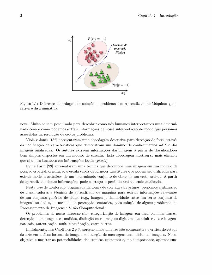
abordagens principais: generativa e discriminativa [146].
Com a abordagem generativa, procuramos resolver um problema dando enfase no processo
de geracao dos dados sob analise. Normalmente, modelamos o sistema como uma distribuicao
conjunta de probabilidade (Joint probability function) e, desta forma, podemos criar exemplos
artificiais que podem ser inseridos no sistema. Exemplos de modelos que utilizam a abordagem
generativa sao: Classificadores Bayesianos, Markov Random Fields e Gaussian Mixture Mo-
dels [55]. Por outro lado, na abordagem discriminativa, procuramos encontrar as fronteiras que
melhor separam um conjunto de classes do nosso problema. Classificadores como Support Vector
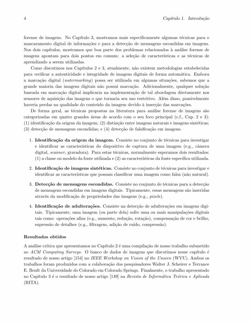
Machines (SVMs) [31] utilizam esta abordagem. Para entender melhor, considere a Figura 1.1.
Nesse problema de classificacao, a abordagem generativa objetiva encontrar relacoes metricas na
classe dos cırculos (+1) e dos triangulos (−1), de modo a modelar o processo de geracao desses
dados. Em contrapartida, a abordagem discriminativa procura modelar a melhor fronteira de
separacao das duas classes.
De forma geral, os modelos generativo e discriminativo podem variar de acordo com cada
aplicacao. Nesta pesquisa de doutorado, nos avaliamos e aplicamos a melhor abordagem de
acordo com o problema analisado. Em alguns casos, pode ser necessario utilizar uma associacao
destas duas abordagens [69] construindo um modelo de extracao/classificacao de caracterısticas
mais robusto.
A associacao de informacoes aprendidas a partir de um conjunto de dados nao e uma ideia
1
2 Capıtulo 1. Introducao
Figura 1.1: Diferentes abordagens de solucao de problemas em Aprendizado de Maquina: gene-rativa e discriminativa.
nova. Muito se tem pesquisado para descobrir como nos humanos interpretamos uma determi-
nada cena e como podemos extrair informacoes de nossa interpretacao de modo que possamos
associa-las na resolucao de certos problemas.
Viola e Jones [182] apresentaram uma abordagem descritiva para deteccao de faces atraves
da codificacao de caracterısticas que demonstram um domınio de conhecimentos ad hoc das
imagens analisadas. Os autores extraem informacoes das imagens a partir de classificadores
bem simples dispostos em um modelo de cascata. Esta abordagem mostrou-se mais eficiente
que sistemas baseados em informacoes locais (pixels).
Lyu e Farid [99] apresentaram uma tecnica que decompoe uma imagem em um modelo de
posicao espacial, orientacao e escala capaz de fornecer descritores que podem ser utilizados para
extrair modelos artısticos de um determinado conjunto de obras de um certo artista. A partir
do aprendizado dessas informacoes, pode-se tracar o perfil do artista sendo analisado.
Nesta tese de doutorado, organizada na forma de coletanea de artigos, propomos a utilizacao
de classificadores e tecnicas de aprendizado de maquina para extrair informacoes relevantes
de um conjunto generico de dados (e.g., imagens), similaridade entre um certo conjunto de
imagens ou dados, ou mesmo sua percepcao semantica, para solucao de alguns problemas em
Processamento de Imagens e Visao Computacional.
Os problemas de nosso interesse sao: categorizacao de imagens em duas ou mais classes,
deteccao de mensagens escondidas, distincao entre imagens digitalmente adulteradas e imagens
naturais, autenticacao, multi-classificacao, entre outros.
Inicialmente, nos Capıtulos 2 e 3, apresentamos uma revisao comparativa e crıtica do estado
da arte em analise forense de imagens e deteccao de mensagens escondidas em imagens. Nosso
objetivo e mostrar as potencialidades das tecnicas existentes e, mais importante, apontar suas

1.1. Deteccao de adulteracoes em imagens digitais 3
limitacoes. Com esse estudo, mostramos que boa parte dos problemas nessa area apontam
para dois pontos em comum: a selecao de caracterısticas e as tecnicas de aprendizado a serem
utilizadas. Nesse estudo, tambem discutimos questoes legais associadas a analise forense de
imagens como, por exemplo, o uso de fotografias digitais por criminosos.
Em seguida, no Capıtulo 4, introduzimos uma tecnica para analise forense de imagens tes-
tada no contexto de deteccao de mensagens escondidas e de classificacao geral de imagens em
categorias como indoors, outdoors, geradas em computador e obras de arte.
Ao estudarmos esse problema de multi-classificacao, surgem algumas questoes: como re-
solver um problema multi-classe de modo a poder combinar, por exemplo, caracterısticas de
classificacao de imagens baseadas em cor, textura, forma e silhueta, sem nos preocuparmos de-
masiadamente em como normalizar o vetor-comum de caracterısticas gerado? Como utilizar
diversos classificadores diferentes, cada um, especializado e melhor configurado para um con-
junto de caracterısticas ou classes em confusao? Nesse sentido, no Capıtulo 5, apresentamos
uma tecnica para fusao de classificadores e caracterısticas no cenario multi-classe atraves da
combinacao de classificadores binarios. Nos validamos nossa abordagem numa aplicacao real
para classificacao automatica de frutas e legumes.
Finalmente, nos deparamos com mais um problema interessante: como tornar a utilizacao
de poderosos classificadores binarios no contexto multi-classe mais eficiente e eficaz? Assim, no
Capıtulo 6, introduzimos uma tecnica para combinacao de classificadores binarios (chamados
classificadores base) para a resolucao de problemas no contexto geral de multi-classificacao.
No restante do Capıtulo 1, apresentamos um resumo de nossas contribuicoes nesse trabalho
de doutorado. Os capıtulos posteriores apresentam mais detalhes sobre cada uma das contri-
buicoes. Antes de cada capıtulo, apresentamos um breve resumo, em portugues, sobre o assunto
a ser tratado e, em seguida, apresentamos o capıtulo em ingles. Ao final, apresentamos as
consideracoes finais de nosso trabalho.
1.1 Deteccao de adulteracoes em imagens digitais
Ao campo de pesquisas relacionado a analise de imagens para verificacao de sua autenticidade e
integridade denominamos Analise Forense de Imagens. Com o advento da internet e das cameras
de alta performance e de baixo custo juntamente com poderosos pacotes de software de edicao
de imagens (Photoshop, Adobe Illustrator, Gimp), usuarios comuns tornaram-se potenciais es-
pecialistas na criacao e manipulacao de imagens digitais. Quando estas modificacoes deixam de
ser inocentes e passam a implicar em questoes legais, torna-se necessario o desenvolvimento de
abordagens eficientes e eficazes para sua deteccao.
A identificacao de imagens que foram digitalmente adulteradas e de fundamental importancia
atualmente [43,138,141]. O julgamento de um crime, por exemplo, pode estar sendo baseado em
evidencias que foram fabricadas especificamente para enganar e mudar a opiniao de um juri. Um
polıtico pode ter a opiniao publica lancada contra ele por ter aparecido ao lado de um traficante
procurado mesmo sem nunca ter visto este traficante antes.
No Capıtulo 2, apresentamos um estudo crıtico das principais tecnicas existentes na analise
4 Capıtulo 1. Introducao
forense de imagens. No Capıtulo 3, mostramos mais especificamente algumas tecnicas para o
mascaramento digital de informacoes e para a deteccao de mensagens escondidas em imagens.
Nos dois capıtulos, mostramos que boa parte dos problemas relacionados a analise forense de
imagens apontam para dois pontos em comum: a selecao de caracterısticas e as tecnicas de
aprendizado a serem utilizadas.
Como discutimos nos Capıtulos 2 e 3, atualmente, nao existem metodologias estabelecidas
para verificar a autenticidade e integridade de imagens digitais de forma automatica. Embora
a marcacao digital (watermarking) possa ser utilizada em algumas situacoes, sabemos que a
grande maioria das imagens digitais nao possui marcacao. Adicionalmente, qualquer solucao
baseada em marcacao digital implicaria na implementacao de tal abordagem diretamente nos
sensores de aquisicao das imagens o que tornaria seu uso restritivo. Alem disso, possivelmente
haveria perdas na qualidade do conteudo da imagem devido a insercao das marcacoes.
De forma geral, as tecnicas propostas na literatura para analise forense de imagens sao
categorizadas em quatro grandes areas de acordo com o seu foco principal (c.f., Cap. 2 e 3):
(1) identificacao da origem da imagem; (2) distincao entre imagens naturais e imagens sinteticas;
(3) deteccao de mensagens escondidas; e (4) deteccao de falsificacao em imagens.
1. Identificacao da origem da imagem. Consiste no conjunto de tecnicas para investigar
e identificar as caracterısticas do dispositivo de captura de uma imagem (e.g., camera
digital, scanner, gravadora). Para estas tecnicas, normalmente esperamos dois resultados:
(1) a classe ou modelo da fonte utilizada e (2) as caracterısticas da fonte especıfica utilizada.
2. Identificacao de imagens sinteticas. Consiste no conjunto de tecnicas para investigar e
identificar as caracterısticas que possam classificar uma imagem como falsa (nao natural).
3. Deteccao de mensagens escondidas. Consiste no conjunto de tecnicas para a deteccao
de mensagens escondidas em imagens digitais. Tipicamente, essas mensagens sao inseridas
atraves da modificacao de propriedades das imagens (e.g., pixels).
4. Identificacao de adulteracoes. Consiste na deteccao de adulteracoes em imagens digi-
tais. Tipicamente, uma imagem (ou parte dela) sofre uma ou mais manipulacoes digitais
tais como: operacoes afins (e.g., aumento, reducao, rotacao), compensacao de cor e brilho,
supressao de detalhes (e.g., filtragem, adicao de ruıdo, compressao).
Resultados obtidos
A analise crıtica que apresentamos no Capıtulo 2 e uma compilacao de nosso trabalho submetido
ao ACM Computing Surveys. O banco de dados de imagens que discutimos nesse capıtulo e
resultado de nosso artigo [154] no IEEE Workshop on Vision of the Unseen (WVU). Ambos os
trabalhos foram produzidos com a colaboracao dos pesquisadores Walter J. Scheirer e Terrance
E. Boult da Universidade do Colorado em Colorado Springs. Finalmente, o trabalho apresentado
no Capıtulo 3 e o resultado de nosso artigo [149] na Revista de Informatica Teorica e Aplicada
(RITA).
1.2. Esteganalise e categorizacao de imagens 5
1.2 Esteganalise e categorizacao de imagens
Pequenas perturbacoes feitas nos canais menos significativos de imagens digitais (e.g., canal LSB)
sao imperceptıveis aos humanos mas sao estatisticamente detectaveis no contexto de analise de
imagens [147,188].
Nesse sentido, no Capıtulo 4, apresentamos uma abordagem para meta-descricao de imagens
denominada Randomizacao Progressiva (PR1) para nos auxiliar nos problemas de: (1) Deteccao
de mensagens escondidas em imagens digitais; e (2) Categorizacao de imagens.
1.2.1 Deteccao de mensagens escondidas
Neste problema, procuramos aperfeicoar e dar robustez ao trabalho desenvolvido em meu mes-
trado [35]. Estudamos e desenvolvemos tecnicas capazes de permitir a deteccao de mensagens
escondidas em imagens digitais.
Grande parte das tecnicas de esteganografia, a arte das comunicacoes escondidas, possuem fa-
lhas e/ou inserem artefatos (padroes) detectaveis nos objetos de cobertura (utilizados para escon-
der uma determinada mensagem). A identificacao destes artefatos e sua correta utilizacao na de-
teccao de mensagens escondidas constituem a arte e a ciencia conhecida como esteganalise [149].
O metodo de randomizacao progressiva proposto permite a deteccao de mensagens escondidas
em imagens com compressao sem perdas (e.g., PNGs). Alem disso, o metodo permite apontar
quais os tipos de imagens sao mais sensıveis ao mascaramento de mensagens bem como quais
tipos de imagens sao mais propıcios a este tipo de operacoes.
1.2.2 Categorizacao de imagens – Cenario de duas classes
O conhecimento semantico sobre uma determinada mıdia nos permite desenvolver tecnicas inteli-
gentes de processamento dessas mıdias baseadas em seu conteudo. Cameras digitais ou aplicacoes
de computador podem corrigir cor e brilho automaticamente levando em consideracao propri-
edades da cena analisada. Nesses casos, informacoes locais das mıdias podem ser insuficientes
para determinados problemas.
Nesse trabalho de doutorado, procuramos desenvolver uma tecnica capaz de associar in-
formacoes coletadas atraves de relacoes encontradas em um grande banco de dados de imagens
para separar imagens naturais de imagens geradas em computador [37, 98, 119], imagens em
ambiente externo (outdoors) de imagens em ambiente interno (indoors) [92,128,162], e imagens
naturais de imagens de obras de arte [34]. Nossa abordagem consiste em capturar propriedades
estatısticas das duas classes analisadas de cada vez e buscar diferencas nestas propriedades.
1.2.3 Categorizacao de imagens – Cenario multi-classe
Denomina-se categorizacao de imagens ao conjunto de tecnicas que distinguem classes de ima-
gens, apontando o tipo de uma imagem. Nesse problema, objetivamos desenvolver uma abor-
1Originalmente, denominamos nosso meta-descritor como Progressive Randomization (PR).

6 Capıtulo 1. Introducao
dagem de categorizacao de imagens para as classes indoors, outdoors, geradas em computador e
artes. Nao consideramos classes especıficas de objetos tais como carros ou pessoas. Um cenario
tıpico para uma aplicacao e o agrupamento de fotos em albuns automaticamente de acordo com
classes. A solucao que apresentamos e simples, unificada e relativamente possui baixa dimensi-
onalidade2.
1.2.4 Randomizacao Progressiva (PR)
PR e um novo meta-descritor que captura as diferencas entre classes gerais de imagens usando
os artefatos estatısticos inseridos durante um processo de perturbacao sucessiva das imagens
analisadas. Nossos experimentos demonstraram que esta tecnica captura bem a separabilidade
de algumas classes de imagens. A observacao mais importante e que classes diferentes de imagens
possuem comportamentos distintos quando submetidas a sucessivas perturbacoes. Por exemplo,
um conjunto de imagens que nao possui mensagens escondidas apresenta diferentes artefatos
mediante sucessivas perturbacoes que um conjunto de imagens que possui mensagens escondidas.
No Algoritmo 1, resumimos os quatro passos principais da Randomizacao Progressiva apli-
cada a Esteganalise e a Categorizacao de Imagens. Os quatro passos sao: (1) o processo de
randomizacao; (2) selecao de regioes caracterısticas; (3) descricao estatıstica; e (4) invariancia.
Algorithm 1 Meta-descritor de Randomizacao Progressiva (PR).
Require: Imagem de entrada I; Porcentagens P = P1, . . . Pn;1: Randomizacao: faca n perturbacoes nos bits menos significativos de I
Oii=0...n. = I, T (I, P1), . . . , T (I, Pn).
2: Selecao de regioes: selecione r regioes de cada imagem i ∈ Oii=0...n
Oij i = 0 . . . n,
j = 1 . . . r.
= O01, . . . , Onr.
3: Descricao estatıstica: calcule m descritores estatısticos para cada regiao
dijk = dk(Oij) i = 0 . . . n,
j = 1 . . . r,
k = 1 . . . m.
4: Invariancia: normalize os descritores de acordo com seus valores na imagem de entrada I
F = fee=1...n×r×m =
dijk
d0jk
i = 0 . . . n,
j = 1 . . . r,
k = 1 . . . m.
,
5: Use as caracterısticas dijk ∈ R(n+1)×r×m (nao-normalizadas) ou dijk ∈ R
n×r×m (nor-malizadas) em seu classificador de padroes favorito.
2Baixa dimensionalidade refere-se a um baixo numero de caracterısticas no processo de descricao dos elementosanalisados.
1.2. Esteganalise e categorizacao de imagens 7
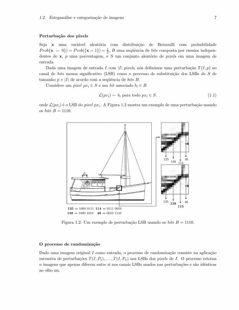
Perturbacao dos pixels
Seja x uma variavel aleatoria com distribuicao de Bernoulli com probabilidade
Probx = 0) = Prob(x = 1) = 12 , B uma sequencia de bits composta por ensaios indepen-
dentes de x, p uma porcentagem, e S um conjunto aleatorio de pixels em uma imagem de
entrada.
Dada uma imagem de entrada I com |I| pixels, nos definimos uma perturbacao T (I, p) no
canal de bits menos significativo (LSB) como o processo de substituicao dos LSBs de S de
tamanho p× |I| de acordo com a sequencia de bits B.
Considere um pixel pxi ∈ S e um bit associado bi ∈ B
L(pxi)← bi para todo pxi ∈ S. (1.1)
onde L(pxi) e o LSB do pixel pxi. A Figura 1.2 mostra um exemplo de uma perturbacao usando
os bits B = 1110.
135 = 1000 0111
138 = 1000 1010
114 = 0111 0010
46 = 0010 1110
135138 114
46
135139
115
46
Figura 1.2: Um exemplo de perturbacao LSB usando os bits B = 1110.
O processo de randomizacao
Dado uma imagem original I como entrada, o processo de randomizacao consiste na aplicacao
sucessiva de perturbacoes T (I, P1), . . . , T (I, Pn) nos LSBs dos pixels de I. O processo retorna
n imagens que apenas diferem entre si nos canais LSBs usados nas perturbacoes e sao identicas
ao olho nu.

8 Capıtulo 1. Introducao
As T (I, Pi) transformacoes sao perturbacoes de diferentes porcentagens (pesos) nos LSBs dis-
ponıveis. Em nosso trabalho base, utilizamos n = 6 onde P = 1%, 5%, 10%, 25%, 50%, 75%,Pi ∈ P denota os tamanhos relativos dos conjuntos de pixels selecionados S.
Selecao de regioes
Propriedades locais nao aparecem diretamente sob uma investigacao global [188]. Nos utilizamos
descritores estatısticos em regioes locais para capturar as mudancas inseridas pelas perturbacoes
sucessivas (c.f., Sec. 1.2.4).
Dada uma imagem I, nos usamos r regioes com tamanho l×l pixels para produzir descritores
estatısticos localizados. Na Figura 1.3, nos mostramos uma configuracao com r = 8 regioes com
sobreposicao de informacoes.
Figura 1.3: Oito regioes de interesse considerando sobreposicao de informacoes.
Descricao estatıstica
As perturbacoes LSB mudam o conteudo de um conjunto selecionado de pixels e induzem mu-
dancas localizadas nas estatısticas dos pixels. Um pixel com L bits possui 2L valores possıveis
e representa 2L−1 classes de invariancia se consideramos possıveis mudancas apenas no canal
LSB (c.f., Sec. 1.2.4). Chamamos estas classes de invariancia de pares de valores (PoV3).
Quando perturbamos todos os LSBs disponıveis em S com uma sequencia B, a distribuicao
de valores 0/1 de um PoV sera a mesma de B. A analise estatıstica compara os valores teoricos
esperados com os observados dos PoVs apos o processo de perturbacao.
Nos aplicamos os descritores estatısticos χ2 (Teste do Chi-quadrado) [191] e UT (Teste Uni-
versal de Ueli Maurer) [102] para analisar estas mudancas.
3Pair of Values.

1.3. Fusao multi-classe de caracterısticas e classificadores 9
Invariancia
Em algumas situacoes, e necessario usar um descritor de caracterısticas invariante. Para tal, usa-
mos a taxa de variacao de nossos descritores estatısticos em relacao a cada perturbacao sucessiva,
ao inves de seus valores diretos. Nos normalizamos todos os valores de descritores decorrentes
das transformacoes em relacao aos seus valores na imagem de entrada (sem perturbacao)
F = fee=1...n×r×m =
dijk
d0jk
i = 0 . . . n,
j = 1 . . . r,
k = 1 . . . m.
, (1.2)
onde d denota um descritor 1 ≤ k ≤ m de uma regiao 1 ≤ j ≤ r de uma imagem 0 ≤ i ≤ n e F
e o vetor de caracterısticas final gerado para a imagem I.
A necessidade da etapa de invariancia depende da aplicacao. Por exemplo, ela e necessaria
no contexto de deteccao de mensagens escondidas uma vez que queremos diferenciar imagens que
contem mensagens escondidas daquelas que nao contem. A classe das imagens nao e relevante.
No contexto de categorizacao de imagens, os valores em si sao mais importantes que a taxa de
variabilidade em perturbacoes sucessivas.
1.2.5 Resultados obtidos
O Capıtulo 4 e uma compilacao de nosso trabalho submetido a Elsevier Computer Vision and
Image Understanding (CVIU). Apos um estudo que mostrou viabilidade comercial de nossa
tecnica, conseguimos o deposito de uma patente nacional4 junto ao INPI5 e sua versao interna-
cional6 junto ao PCT7.
Finalmente, o trabalho de deteccao de mensagens nos rendeu a publicacao [147] no IEEE
Intl. Workshop on Multimedia and Signal Processing (MMSP). A extensao da tecnica para
o cenario multi-classe (indoors, outdoors, geradas em computador, e obras de arte) resultou o
artigo [148] no IEEE Intl. Conference on Computer Vision (ICCV).
1.3 Fusao multi-classe de caracterısticas e classificadores
Algumas vezes, problemas de categorizacao multi-classe sao complexos e a fusao de informacoes
de varios descritores torna-se importante.
Embora a fusao de caracterısticas seja bastante eficaz para alguns problemas, ela pode produ-
zir resultados inesperados quando as diferentes caracterısticas nao estao normalizadas e prepara-
das de forma adequada. Alem disso, esse tipo de combinacao tem a desvantagem de aumentar o
numero de caracterısticas do vetor base de descricao o que, por sua vez, pode levar a necessidade
de mais elementos para o treinamento.
4http://www.inovacao.unicamp.br/report/patentes_ano2006-inova.pdf5Instituto Nacional de Propriedade Industrial.6http://www.inovacao.unicamp.br/report/inte-allpatentes2007-unicamp071228.pdf7Patent Cooperation Treaty.

10 Capıtulo 1. Introducao
Alem disso, em certas ocasioes, alguns classificadores produzem melhores resultados para
determinados descritores do que para outros. Isto sugere que a combinacao de classificadores
em problemas multi-classe, cada um especializado em um caso particular, pode ser interessante.
Embora a combinacao de classificadores e caracterısticas nao seja tao direta no cenario
multi-classe, ela e um problema simples para problemas de classificacao binarios. Nesse caso, e
possıvel combinar diferentes classificadores e caracterısticas usando regras simples de fusao tais
como and, or, max, sum, ou min [16]. No entanto, para problemas multi-classe, a fusao torna-se
um pouco mais complicada dado que uma caracterıstica pode apontar como resultado a classe
Ci, outra caracterıstica apontar a classe Cj, e ainda outra poderia produzir o resultado Ck.
Com muitos resultados diferentes para um mesmo exemplo de teste, torna-se difıcil definir uma
polıtica consistente para combinar as caracterısticas selecionadas.
Uma abordagem muito usada consiste na combinacao dos vetores caracterısticos em um
grande vetor de descricao. Embora bem eficaz em alguns casos, esta abordagem pode, tambem,
produzir resultados inesperados quando o vetor nao e normalizado e preparado da forma ade-
quada. Em primeiro lugar, para criar o vetor combinado de caracterısticas, precisamos lidar
com a natureza diferente de cada vetor caracterıstico. Alguns podem ser bem condicionados
possuindo apenas variaveis contınuas e limitadas, outros podem ser mal-condicionados para
essa combinacao tais como aqueles que possuem variaveis categoricas. Adicionalmente, algumas
variaveis podem ser contınuas e nao limitadas. Em resumo, para unificar todas as caracterısticas,
precisamos de um pre-processamento e normalizacao adequados. Entretanto, algumas vezes esse
pre-processamento e trabalhoso.
Esse tipo de combinacao de caracterısticas eventualmente pode levar a maldicao da dimen-
sionalidade. Dado que temos mais dimensoes no vetor caracterıstico combinado, precisamos de
mais exemplos de treinamento.
Finalmente, se precisarmos adicionar mais uma caracterıstica aquelas existentes, temos que
pre-processar os dados novamente para uma nova normalizacao.
1.3.1 Solucao proposta
No Capıtulo 5, nos apresentamos uma abordagem para combinar classificadores e caracterısticas
capaz de lidar com a maior parte dos problemas citados anteriormente. Nosso objetivo e combi-
nar um conjunto de caracterısticas e os classificadores mais apropriados para cada uma de modo
a melhorar a performance sem comprometer a eficiencia.
Nos propomos lidar com um problema multi-classe a partir da combinacao de um conjunto de
classificadores binarios. Podemos definir a binarizacao de classes como um mapeamento de um
problema multi-classe para varios problemas binarios (dividir para conquistar) e a subsequente
combinacao de seus resultados para derivar a predicao multi-classe. Nos referimos aos classifica-
dores binarios como classificadores base. A binarizacao de classes tem sido utilizada na literatura
para estender classificadores naturalmente binarios tais como SVM para multi-classe [5,38,115].
Entretanto, de acordo com nosso conhecimento, esta abordagem nao foi utilizada anteriormente
para a fusao de classificadores e caracterısticas.

1.3. Fusao multi-classe de caracterısticas e classificadores 11
Para entender a binarizacao de classes, considere um problema com tres classes. Nesse caso,
uma binarizacao simples consiste no treinamento de tres classificadores binarios. Nesse sentido,
nos precisamos O(N2) classificadores base, onde N e o numero de classes.
Nos treinamos o ijesimo classificador binario utilizando os padroes da classe i como positivos
e os padroes da classe j como negativos. Para obter o resultado final, calculamos a distancia
mınima do vetor binario gerado para o padrao binario que representa cada classe.
Considere novamente o exemplo com tres classes como mostramos na Figura 1.4. Nesse
exemplo, nos temos as classes: Triangulos , Cırculos ©, e Quadrados 2. Claramente, uma
primeira caracterıstica que podemos usar para categorizar os elementos dessas classes pode ser
baseado na forma. Podemos tambem utilizar propriedades de cor e textura. Para resolver esse
problema, treinamos alguns classificadores binarios diferenciando duas classes por vez, tais como:
ש, × 2, e ©× 2. Adicionalmente, nos representamos cada uma das classes com um
identificador unico ( = 〈+1, +1, 0〉).
Figura 1.4: Pequeno exemplo para combinacao de classificadores e caracterısticas.
Ao recebermos um exemplo para classificar, digamos um com a forma de triangulo, como
mostramos na Figura 1.4, primeiro aplicamos nossos classificadores binarios para verificar se o
exemplo testado e um triangulo ou um cırculo baseado na forma, textura e cor. Cada classi-
ficador nos da uma resposta binaria. Por exemplo, digamos que nosso resultado seja os votos
〈+1, +1,−1〉 para o classificador binario ש. Dessa forma, nos podemos usar o voto ma-
12 Capıtulo 1. Introducao
joritario e selecionar uma resposta (+1, neste caso, ou ). Entao, repetimos o procedimento
e testamos se o exemplo analisado e um triangulo ou um quadrado para cada uma das carac-
terısticas de interesse. Finalmente, depois de efetuar o ultimo teste, temos como resultado um
vetor binario. Basta entao calcularmos o mınima distancia deste vetor aos vetores identificadores
de cada classe. Nesse exemplo, a resposta final e dada pela mınima distancia de
min dist(〈1, 1,−1〉, 〈1, 1, 0〉, 〈−1, 0, 1〉, 〈0,−1,−1〉). (1.3)
Um aspecto importante dessa abordagem e que ela requer mais armazenamento dado que
apos o treinamento dos classificadores binarios nos precisamos armazenar seus parametros. Dado
que nos analisamos mais caracterısticas, precisamos de mais espaco. Com respeito ao tempo de
execucao, tem tambem um crescimento dado que precisamos testar mais classificadores binarios
para obter uma resposta. Entretanto, muitos classificadores em nosso dia-a-dia empregam algum
tipo de binarizacao de classes (e.g., SVMs). Alem disso, como apresentamos no Capıtulo 6,
existem solucoes efetivas para combinar tais classificadores binarios de forma eficiente.
Embora precisemos de mais espaco de armazenamento, a abordagem apresentada tem as
seguintes vantagens:
1. Com a combinacao independente de caracterısticas, temos mais confianca na resposta
produzida dado que ela e calculada a partir de mais de uma simples caracterıstica. Dessa
forma, temos um mecanismo simples de correcao de erros que pode resistir a algumas
classificacoes erradas;
2. Podemos desenvolver classificadores e caracterısticas especıficas para separar classes em
confusao;
3. Podemos selecionar as caracterısticas que realmente sao importantes na fusao. Esse proce-
dimento nao e direto quando temos apenas um grande vetor de caracterısticas combinadas.
4. A adicao de novas classes requer apenas o treinamento para os novos classificadores binarios
relacionados aquelas classes.
5. A adicao de novas caracterısticas e simples e requer apenas treinamento parcial.
6. Como nao aumentamos o tamanho de nenhum vetor de caracterısticas, temos menor pro-
babilidade de sofrermos da maldicao da dimensionalidade, nao necessitando, portanto,
adicionar mais exemplos de treinamento quando combinando mais caracterısticas.
Finalmente, nos validamos nossa abordagem de fusao de classificadores e caracterısticas
numa aplicacao real para categorizacao automatica de frutas e legumes, como apresentamos no
Capıtulo 5.

1.4. Multi-classe a partir de classificadores binarios 13
1.3.2 Resultados obtidos
O Capıtulo 5 e uma compilacao de nosso trabalho submetido a Elsevier Computers and Electro-
nics in Agriculture (Compag) e do artigo [153] no Brazilian Symposium of Computer Graphics
and Image Processing (Sibgrapi). Esses trabalhos foram produzidos com a colaboracao dos
pesquisadores Daniel C. Hauagge e Jacques Wainer do Instituto de Computacao da Unicamp.
1.4 Multi-classe a partir de classificadores binarios
Muitos problemas reais de reconhecimento e de classificacao frequentemente necessitam ma-
pear varias entradas em uma dentre centenas ou milhares de possıveis categorias. Muitos pes-
quisadores tem proposto tecnicas efetivas para classificacao de duas classes nos ultimos anos.
No entanto, alguns classificadores poderosos tais como SVMs sao difıceis de estender para o
cenario multi-classe. Em tais casos, a abordagem mais comum e a de reduzir a complexidade do
problema multi-classe para pequenos e mais simples problemas binarios (dividir para conquis-
tar) [38,82,127,145].
Ao utilizar classificadores binarios com algum criterio final de combinacao (reducao de com-
plexidade), muitas abordagens descritas na literatura partem do princıpio de que os classificado-
res binarios utilizados na classificacao sao independentes e aplicam um sistema de votacao como
polıtica final de combinacao. Entretanto, a hipotese da independencia nao e a melhor escolha
em todos os casos.
Nesse trabalho, nos abordamos o problema de classificacao multi-classe apresentando uma
forma efetiva de agrupar dicotomias altamente correlacionadas (nao supondo independencia
entre todas elas). Nos denominamos a tecnica de Affine-Bayes (c.f., Sec. 1.4.1).
1.4.1 Affine-Bayes
Apresentamos, a seguir, nossa abordagem generativa Bayesiana para multi-classificacao. Um
problema multi-classe tıpico resolvido a partir da combinacao de classificadores binarios possui
tres etapas basicas [145]: (1) a criacao da matriz de codificacao dos classificadores; (2) a escolha
dos classificadores binarios base; e (3) a estrategia de decodificacao. A solucao que propomos
enquadra-se, principalmente, na parte 3.
Considerando a etapa de decodificacao, nos introduzimos o conceito de relacoes afins entre
classificadores binarios e apresentamos uma abordagem efetiva para achar grupos de classifi-
cadores binarios altamente correlacionados. Finalmente, apresentamos duas novas estrategias:
uma para reduzir o numero necessario de dicotomias na classificacao multi-classe e a outra para
achar novas dicotomias para substituir aquelas menos discriminativas. Esses dois procedimentos
podem ser utilizados iterativamente para complementar a abordagem basica de Affine-Bayes e
melhorar a performance geral de classificacao.
Para classificar uma determinada entrada, nos usamos um time de classificadores binarios
base T . Nos chamamos OT uma realizacao de T . Cada elemento de T e um classificador binario
base (dicotomia) e produz uma saıda ∈ −1, +1.
14 Capıtulo 1. Introducao
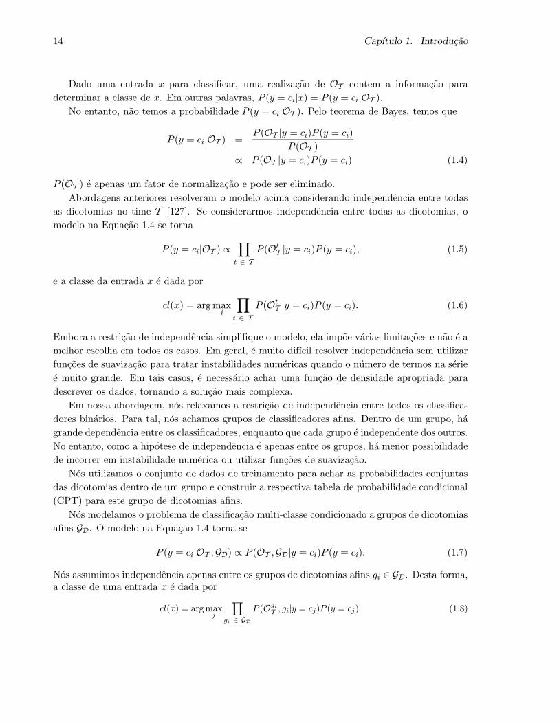
Dado uma entrada x para classificar, uma realizacao de OT contem a informacao para
determinar a classe de x. Em outras palavras, P (y = ci|x) = P (y = ci|OT ).
No entanto, nao temos a probabilidade P (y = ci|OT ). Pelo teorema de Bayes, temos que
P (y = ci|OT ) =P (OT |y = ci)P (y = ci)
P (OT )
∝ P (OT |y = ci)P (y = ci) (1.4)
P (OT ) e apenas um fator de normalizacao e pode ser eliminado.
Abordagens anteriores resolveram o modelo acima considerando independencia entre todas
as dicotomias no time T [127]. Se considerarmos independencia entre todas as dicotomias, o
modelo na Equacao 1.4 se torna
P (y = ci|OT ) ∝∏
t ∈ T
P (OtT |y = ci)P (y = ci), (1.5)
e a classe da entrada x e dada por
cl(x) = arg maxi
∏
t ∈ T
P (OtT |y = ci)P (y = ci). (1.6)
Embora a restricao de independencia simplifique o modelo, ela impoe varias limitacoes e nao e a
melhor escolha em todos os casos. Em geral, e muito difıcil resolver independencia sem utilizar
funcoes de suavizacao para tratar instabilidades numericas quando o numero de termos na serie
e muito grande. Em tais casos, e necessario achar uma funcao de densidade apropriada para
descrever os dados, tornando a solucao mais complexa.
Em nossa abordagem, nos relaxamos a restricao de independencia entre todos os classifica-
dores binarios. Para tal, nos achamos grupos de classificadores afins. Dentro de um grupo, ha
grande dependencia entre os classificadores, enquanto que cada grupo e independente dos outros.
No entanto, como a hipotese de independencia e apenas entre os grupos, ha menor possibilidade
de incorrer em instabilidade numerica ou utilizar funcoes de suavizacao.
Nos utilizamos o conjunto de dados de treinamento para achar as probabilidades conjuntas
das dicotomias dentro de um grupo e construir a respectiva tabela de probabilidade condicional
(CPT) para este grupo de dicotomias afins.
Nos modelamos o problema de classificacao multi-classe condicionado a grupos de dicotomias
afins GD. O modelo na Equacao 1.4 torna-se
P (y = ci|OT ,GD) ∝ P (OT ,GD|y = ci)P (y = ci). (1.7)
Nos assumimos independencia apenas entre os grupos de dicotomias afins gi ∈ GD. Desta forma,a classe de uma entrada x e dada por
cl(x) = arg maxj
∏
gi ∈ GD
P (Ogi
T, gi|y = cj)P (y = cj). (1.8)

1.4. Multi-classe a partir de classificadores binarios 15
Para achar os grupos de classificadores binarios afins GD, nos definimos uma matriz de
afinidade A entre os classificadores. Esta matriz indica quao afins (correlacionadas) sao duas
dicotomias quando classificando um conjunto de dados de treinamento X. Se as dicotomias
produzem saıdas todas iguais (diferentes), elas sao correlacionadas e tem alta afinidade. Por
outro lado, se seus resultados sao metade iguais e metade diferentes, elas sao nao-correlacionadas
e, portanto, possuem baixa afinidade.
Apos o calculo da matriz de afinidade A, nos utilizamos um algoritmo de clusterizacao para
achar grupos de classificadores binarios afins emA. Os grupos de classificadores afins podem con-
ter classificadores que nao contribuem muito para o processo geral de classificacao. No processo
de Shrinking, apresentamos um procedimento para identificar as dicotomias menos importan-
tes dentro de um grupo de classificadores binarios afins e elimina-los. Para isso, calculamos a
entropia acumulada de cada grupo testando um elemento do grupo de cada vez. Aqueles que
produzem o menor ganho de informacao sao marcados como menos importantes.
A eliminacao de dicotomias menos importantes nos abre a oportunidade de substituı-las
por outras mais discriminativas. No processo de Augmenting, encontramos novas dicotomias
candidatas para repor aquelas eliminadas na etapa de Shrinking. Para isso, analisamos a matriz
de confusao calculada durante o treinamento. Em seguida, representamos as classes como um
grafo onde os nos sao os identificadores das classes e as arestas o grau de confusao. A partir do
grafo, conseguimos criar uma hierarquia de classes em confusao. Apos ordenarmos os grupos de
classes de acordo com a sua confusao, achamos o corte de cada subgrafo que nos permite separar
otimamente os nos. Isso nos da conjuntos de dicotomias que representam classes em confusao e
podem ser substitutas daquelas eliminadas no processo de Shrinking.
Finalmente, podemos utilizar as etapas de Shrinking e Augmenting iterativamente de modo
a otimizar ainda mais o algoritmo base do Affine-Bayes.
1.4.2 Resultados obtidos
O Capıtulo 6 e uma compilacao de nosso trabalho submetido a IEEE Transactions on Pattern
Analysis and Machine Intelligence (TPAMI) e do artigo [150] no Intl. Conference on Computer
Vision Theory and Applications (VISAPP).


Deteccao de Adulteracoes em
Imagens Digitais
No Capıtulo 2, apresentamos um estudo crıtico das principais tecnicas existentes na analise
forense de imagens. Discutimos que boa parte dos problemas relacionados a analise forense
apontam para dois pontos em comum: a selecao de caracterısticas e as tecnicas de aprendizado
a serem utilizadas.
Conforme argumentamos, ainda nao existem metodologias estabelecidas para verificar a au-
tenticidade e integridade de imagens digitais de forma automatica.
A identificacao de imagens que foram digitalmente adulteradas e de fundamental importancia
atualmente [43,138,141]. O julgamento de um crime, por exemplo, pode estar sendo baseado em
evidencias que foram fabricadas especificamente para enganar e mudar a opiniao de um juri. Um
polıtico pode ter a opiniao publica lancada contra ele por ter aparecido ao lado de um traficante
procurado mesmo sem nunca ter visto este traficante antes. Dessa forma, discutimos tambem
questoes legais associadas a analise forense de imagens como, por exemplo, o uso de fotografias
digitais por criminosos.
O trabalho apresentado no Capıtulo 2 e uma compilacao de nosso artigo submetido ao
ACM Computing Surveys. Os autores desse artigo, em ordem, sao: Anderson Rocha, Walter J.
Scheirer, Terrance E. Boult e Siome Goldenstein.
O banco de dados de imagens que discutimos nesse capıtulo e resultado de nosso artigo [154]
no IEEE Workshop on Vision of the Unseen (WVU).
17


Chapter 2
Current Trends and Challenges in
Digital Image Forensics
Abstract
Digital images are everywhere — from our cell phones to the pages of our newspapers. How
we choose to use digital image processing raises a surprising host of legal and ethical questions
we must address. What are the ramifications of hiding data within an innocent image? Is
this security when used legitimately, or intentional deception? Is tampering with an image
appropriate in cases where the image might affect public behavior? Does an image represent a
crime, or is it simply a representation of a scene that has never existed? Before action can even
be taken on the basis of a questionable image, we must detect something about the image itself.
Investigators from a diverse set of fields require the best possible tools to tackle the challenges
presented by the malicious use of today’s digital image processing techniques.
In this paper, we introduce the emerging field of digital image forensics, including the main
topic areas of source camera identification, forgery detection, and steganalysis. In source camera
identification, we seek to identify the particular model of a camera, or the exact camera, that
produced an image. Forgery detection’s goal is to establish the authenticity of an image, or
to expose any potential tampering the image might have undergone. With steganalysis, the
detection of hidden data within an image is performed, with a possible attempt to recover any
detected data. Each of these components of digital image forensics is described in detail, along
with a critical analysis of the state of the art, and recommendations for the direction of future
research.
2.1 Introduction
With the advent of the Internet and low-price digital cameras, as well as powerful image edition
software tools (Adobe Photoshop and Illustrator, GNU Gimp), normal users have become digital
doctoring specialists. At the same time our understanding of the technological, ethical, and
19

20 Chapter 2. Current Trends and Challenges in Digital Image Forensics
legal implications associated with image editing falls far behind. When such modifications are
no longer innocent image tinkerings and start implying legal threats to a society, it becomes
paramount to devise and deploy efficient and effective approaches to detect such activities [141].
Digital Image and Video Forensics research aims at uncovering and analyzing the underlying
facts about an image/video. Its main objectives comprise: tampering detection (cloning, healing,
retouching, splicing), hidden data detection/recovery, and source identification with no prior
measurement or registration of the image (the availability of the original reference image or
video).
Image doctoring in order to represent a scene that never happened is as old as the art
of the photograph itself. Shortly after the Frenchman Nicephore Niepce [29] created the first
photograph in 18141, there were the first indications of doctored photographs. Figure 2.1 depicts
one of the first examples of image forgery. The photograph, an analog composition comprising
30 images2, is known as The Two Ways of Life and was created by Oscar G. Rejland in 1857.
Figure 2.1: Oscar Rejland’s analog composition, 1857.
Though image manipulation is not new, its prevalence in criminal activity has surged over
the past two decades, as the necessary tools have become more readily available, and easier
to use. In the criminal justice arena, we most often find tampered images in connection with
child pornography cases. The 1996 Child Pornography Prevention Act (CPPA) extended the
existing federal criminal laws against child pornography to include certain types of “virtual
porn”. Notwithstanding, in 2002, the United States Supreme Court found that portions of the
CPPA, being excessively broad and restrictive, violated First Amendment rights. The Court
ruled that images containing an actual minor or portions of a minor are not protected, while
computer generated images depicting a fictitious “computer generated” minor are constitution-
ally protected. However, with computer graphics, it is possible to create fake scenes visually
indistinguishable from real ones. In this sense, one can apply sophisticated approaches to give
1Recent studies [101] have pointed out that the photograph was, indeed, invented concurrently by severalresearchers such as Nicephore Niepce, Louis Daguerre, Fox Talbot, and Hercule Florence.
2Available in http://www.bradley.edu/exhibit96/about/twoways.html

2.1. Introduction 21
more realism to the created scenes deceiving the casual eye and conveying a criminal activity.
In the United States, a legal burden exists to “a strong showing of the photograph’s competency
and authenticity3” when such evidence is presented in court. In response, tampering detection
and source identification are tools to satisfy this requirement.
Data hidden within digital imagery represents a new opportunity for classic crimes. Most
notably, the investigation of Juan Carlos Ramirez Abadia, a Columbian drug trafficker arrested
in Brazil in 2008, uncovered voice and text messages hidden within images of a popular cartoon
character4 on the suspect’s computer. Similarly, a 2007 study5 performed by Purdue University
found data hiding tools on numerous computers seized in conjunction with child pornography
and financial fraud cases. While a serious hinderance to a criminal investigation, data hiding is
not a crime in itself; crimes can be masked by its use. Thus, an investigator’s goal here is to
identify and recover any hidden evidence within suspect imagery.
In our digital age, images and videos fly to us at remarkable speed and frequency. Unfortu-
nately, there are currently no established methodologies to verify their authenticity and integrity
in an automatic manner. Digital image and video forensics are still emerging research fields with
important implications for ensuring the credibility of digital contents. As a consequence, on a
daily basis we are faced with numerous images and videos — and it is likely that at least a
few have undergone some level of manipulation. The implications of such tampering are only
beginning to be understood.
Beyond crime, the scientific community has also been subject to these forgeries. A recent
case of scientific fraud involving doctored images in a renowned scientific publication has shed
light to a problem believed to be far from the academy. In 2004, the South Korean professor
Hwang Woo-Suk and colleagues published in Science important results regarding advances in
stem cell research. Less than one year later, an investigative panel pointed out that nine out of
eleven customized stem cell colonies that Hwang had claimed to have made involved doctored
photographs of two other, authentic, colonies. Sadly, this is not a detached case. In at least one
journal6 [129], it is estimated that as many as 20% of the accepted manuscripts contain figures
with improper manipulations, and +1% with fraudulent manipulations [45,129].
Photo and video retouching and manipulation are also present in general press media. On
July 10th, 2008, various major daily newspapers published a photograph of four Iranian missiles
streaking heavenward (see Figure 2.2(a)). Surprisingly, shortly after the photo’s publication,
a small blog provided evidence that the photograph had been doctored. Many of those same
newspapers needed to publish a plethora of retractions and apologies [107].
On March 31st, 2003 the Los Angeles Times showed on its front cover an image from pho-
tojournalist Brian Walki, in which a British soldier in Iraq stood trying to control a crowd
of civilians in a passionate manner. The problem was that the moment depicted never hap-
pened (see Figure 2.2(b)). The photograph was a composite of two different photographs merged
3Bergner v. State, 397 N.E.2d 1012, 1016 (Ind. Ct. App. 1979).4http://afp.google.com/article/ALeqM5ieuIvbrvmfofmOt8o0YfXzbysVuQ5http://www.darkreading.com/security/encryption/showArticle.jhtml?articleID=2088047886Journal of Cell Biology.

22 Chapter 2. Current Trends and Challenges in Digital Image Forensics
to create a more appealing image. The doctoring was discovered and Walski was fired.
In the 2004 presidential campaign, John Kerry’s allies were surprised by a photomontage that
appeared in several newspapers purporting to show Kerry and Jane Fonda standing together at
a podium during a 1970s anti-war rally (see Figure 2.2(c)). As a matter of fact, the photograph
was a fake. Kerry’s picture was taken at an anti-war rally in Mineola, NY., on June 13th, 1971
by photographer Ken Light. Fonda’s picture was taken during a speech at Miami Beach, FL. in
August, 1972 by photographer Owen Franken.
(a) Iranian montage of missiles streaking heav-enward.
(b) Montage of a British soldier in Iraq tryingto control a crowd of civilians in a passionatemanner. Credits to Brian Walski.
(c) Montage of John Kerry and Jane Fonda standing together at a podium during a 1970santi-war rally. Credits to Ken Light (left), AP Photo (middle), and Owen Franken (right).
Figure 2.2: Some common press media photomontages.
It has long been said that an image worth a thousand words. Recently, a study conducted
by Italian Psychologists have investigated how doctored photographs of past public events affect
memory of those events. Their results indicate that doctored photographs of past public events
can influence memory, attitudes and behavioral intentions [158]. That might be one of the
reasons that several dictatorial regimes used to wipe out of their photographic records images
of people who had fallen out of favor with the system [44].
In the following sections, we provide a comprehensive survey of the most relevant works with
respect to this exciting new field of the unseen in digital imagery. We emphasize approaches

2.2. Vision techniques for the Unseen 23
that we believe to be more applicable to forensics. Notwithstanding, most publications in
this emerging field still lack important discussions about resilience to counter-attacks, which
anticipate the existence of forensic techniques [58]. As a result, the question of trustworthiness
of digital forensics arises, for which we try to provide some positive insights.
2.2 Vision techniques for the Unseen
In this section, we survey several state-of-the-art approaches for image and video forgery detec-
tion, pointing out their advantages and limitations.
2.2.1 Image manipulation techniques
In the forensic point of view, it is paramount to distinguish simple image enhancements from
image doctoring. Although there is a thin edge separating both, in the following we try to make
this distinction clear.
On one extreme, we define image enhancements as operations performed in one image with
the intention to improve its visibility. There is no local manipulation or pixel combination. Some
image operations in this category are contrast and brightness adjustments, gamma correction,
scaling, and rotation, among others. On the other extreme, image tampering operations are
those with the intention to deceive the viewer at some level. In these operations, normally one
performs localized image operations such as pixel combinations and tweaks, copy/paste, and
composition with other images. In between these extremes, there are some image operations
that by themselves are not considered forgery creation operations but might be combined for
such objective. Image sharpening, blurring, and compression are some of such operations.
Some common image manipulations with the intention of deceiving a viewer:
1. Composition or splicing. It consists in the composition (merging) of an image Ic using
parts of one or more parts of images I1 . . . Ik. For example, with this approach, a politician
in I1 can be merged beside a person from I2, without even knowing such person.
2. Retouching, healing, cloning. These approaches consist in the alteration of parts of an
image or video using parts or properties of the same image or video. Using such techniques,
one can make a person 10 or 20 years younger (retouching and healing) or even change a
crime scene eliminating a person in a photograph (cloning).
3. Content embedding or Steganography. It consists in the alteration of statistical or
structural properties of images and videos in order to embed hidden contents. Most of the
changes are not visually detectable.
Figure 2.3 depicts some possible image manipulations. From the original image (top left), we
clone several small parts of the same image in order to eliminate some parts of it (for example,
the two people standing in front of the hills). Then we can use a process of smoothing to feather
edges and make the cloning less noticeable. We can use this image as a host for another image
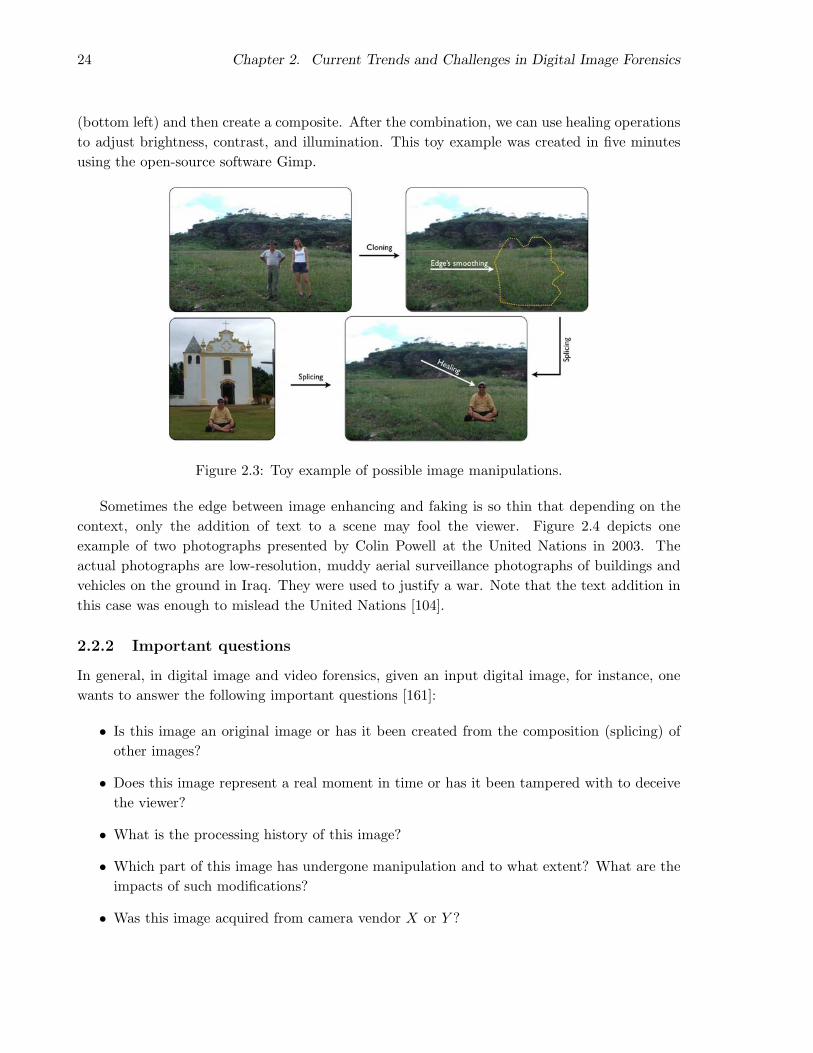
24 Chapter 2. Current Trends and Challenges in Digital Image Forensics
(bottom left) and then create a composite. After the combination, we can use healing operations
to adjust brightness, contrast, and illumination. This toy example was created in five minutes
using the open-source software Gimp.
Figure 2.3: Toy example of possible image manipulations.
Sometimes the edge between image enhancing and faking is so thin that depending on the
context, only the addition of text to a scene may fool the viewer. Figure 2.4 depicts one
example of two photographs presented by Colin Powell at the United Nations in 2003. The
actual photographs are low-resolution, muddy aerial surveillance photographs of buildings and
vehicles on the ground in Iraq. They were used to justify a war. Note that the text addition in
this case was enough to mislead the United Nations [104].
2.2.2 Important questions
In general, in digital image and video forensics, given an input digital image, for instance, one
wants to answer the following important questions [161]:
• Is this image an original image or has it been created from the composition (splicing) of
other images?
• Does this image represent a real moment in time or has it been tampered with to deceive
the viewer?
• What is the processing history of this image?
• Which part of this image has undergone manipulation and to what extent? What are the
impacts of such modifications?
• Was this image acquired from camera vendor X or Y ?

2.2. Vision techniques for the Unseen 25
Figure 2.4: Photographs presented by Colin Powell at the United Nations in 2003. (U.S. De-partment of State)
• Was this image originally acquired with camera C as claimed?
• Does this image conceal any hidden content? Which algorithm or software has been used
to perform the hiding? Is it possible to recover the hidden content?
It is worth noting that most of such techniques are blind and passive. The approach is blind
when it does not use the original content for the analysis. The approach is passive when it does
not use any watermarking-based solution for the analysis.
Although digital watermarking can be used in some situations, the vast majority of digital
contents do not have any digital marking. Any watermarking-based solution would require an
implementation directly in the acquisition sensor, making its use restrictive. Furthermore, such
approaches might lead to quality loss due to the markings [118,161].
We break up the image and video forensics approaches proposed in the literature in three
categories:
1. Camera sensor fingerprinting or source identification;
2. Image and video tampering detection;
3. Image and video hidden content detection/recovery.
2.2.3 Source Camera Identification
With Source Camera Identification, we are interested in identifying the data acquisition device
that generated a given image for forensics purposes. Source camera identification may be bro-
ken into two classes: device class identification and specific device identification. In general,
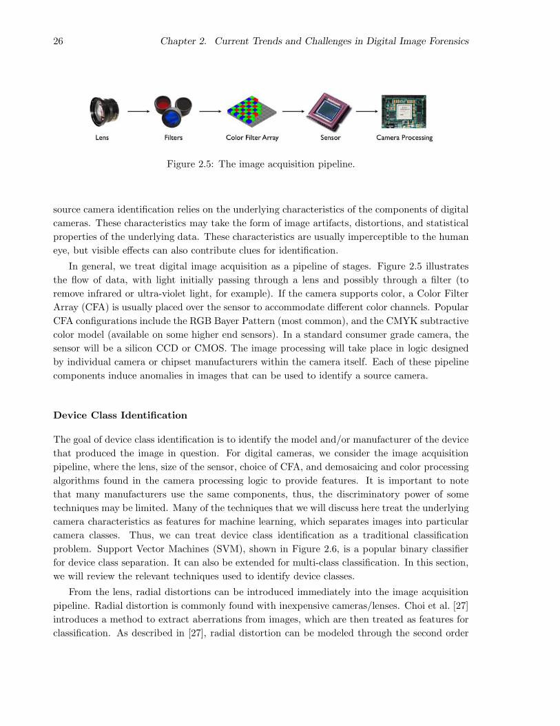
26 Chapter 2. Current Trends and Challenges in Digital Image Forensics
Figure 2.5: The image acquisition pipeline.
source camera identification relies on the underlying characteristics of the components of digital
cameras. These characteristics may take the form of image artifacts, distortions, and statistical
properties of the underlying data. These characteristics are usually imperceptible to the human
eye, but visible effects can also contribute clues for identification.
In general, we treat digital image acquisition as a pipeline of stages. Figure 2.5 illustrates
the flow of data, with light initially passing through a lens and possibly through a filter (to
remove infrared or ultra-violet light, for example). If the camera supports color, a Color Filter
Array (CFA) is usually placed over the sensor to accommodate different color channels. Popular
CFA configurations include the RGB Bayer Pattern (most common), and the CMYK subtractive
color model (available on some higher end sensors). In a standard consumer grade camera, the
sensor will be a silicon CCD or CMOS. The image processing will take place in logic designed
by individual camera or chipset manufacturers within the camera itself. Each of these pipeline
components induce anomalies in images that can be used to identify a source camera.
Device Class Identification
The goal of device class identification is to identify the model and/or manufacturer of the device
that produced the image in question. For digital cameras, we consider the image acquisition
pipeline, where the lens, size of the sensor, choice of CFA, and demosaicing and color processing
algorithms found in the camera processing logic to provide features. It is important to note
that many manufacturers use the same components, thus, the discriminatory power of some
techniques may be limited. Many of the techniques that we will discuss here treat the underlying
camera characteristics as features for machine learning, which separates images into particular
camera classes. Thus, we can treat device class identification as a traditional classification
problem. Support Vector Machines (SVM), shown in Figure 2.6, is a popular binary classifier
for device class separation. It can also be extended for multi-class classification. In this section,
we will review the relevant techniques used to identify device classes.
From the lens, radial distortions can be introduced immediately into the image acquisition
pipeline. Radial distortion is commonly found with inexpensive cameras/lenses. Choi et al. [27]
introduces a method to extract aberrations from images, which are then treated as features for
classification. As described in [27], radial distortion can be modeled through the second order
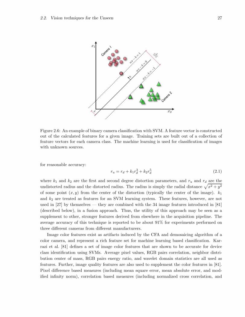
2.2. Vision techniques for the Unseen 27
Figure 2.6: An example of binary camera classification with SVM. A feature vector is constructedout of the calculated features for a given image. Training sets are built out of a collection offeature vectors for each camera class. The machine learning is used for classification of imageswith unknown sources.
for reasonable accuracy:
ru = rd + k1r3d + k2r
5d (2.1)
where k1 and k2 are the first and second degree distortion parameters, and ru and rd are the
undistorted radius and the distorted radius. The radius is simply the radial distance√
x2 + y2
of some point (x, y) from the center of the distortion (typically the center of the image). k1
and k2 are treated as features for an SVM learning system. These features, however, are not
used in [27] by themselves — they are combined with the 34 image features introduced in [81]
(described below), in a fusion approach. Thus, the utility of this approach may be seen as a
supplement to other, stronger features derived from elsewhere in the acquisition pipeline. The
average accuracy of this technique is reported to be about 91% for experiments performed on
three different cameras from different manufacturers.
Image color features exist as artifacts induced by the CFA and demosaicing algorithm of a
color camera, and represent a rich feature set for machine learning based classification. Kar-
razi et al. [81] defines a set of image color features that are shown to be accurate for device
class identification using SVMs. Average pixel values, RGB pairs correlation, neighbor distri-
bution center of mass, RGB pairs energy ratio, and wavelet domain statistics are all used as
features. Further, image quality features are also used to supplement the color features in [81].
Pixel difference based measures (including mean square error, mean absolute error, and mod-
ified infinity norm), correlation based measures (including normalized cross correlation, and
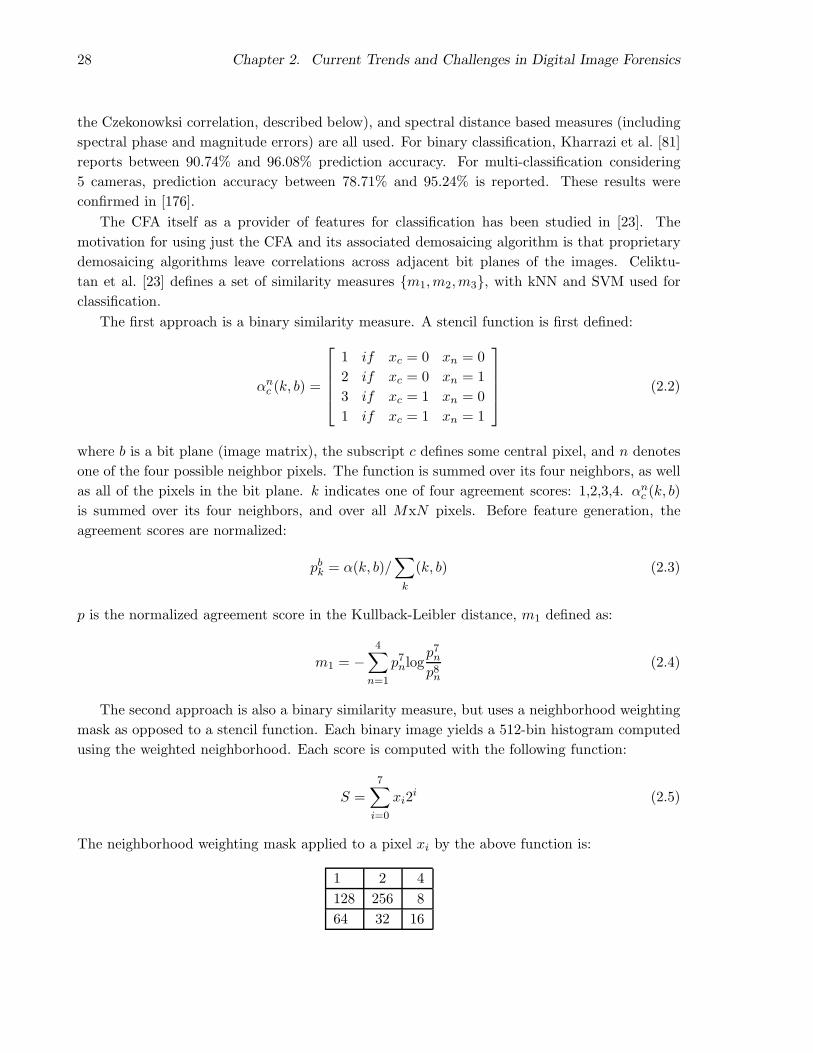
28 Chapter 2. Current Trends and Challenges in Digital Image Forensics
the Czekonowksi correlation, described below), and spectral distance based measures (including
spectral phase and magnitude errors) are all used. For binary classification, Kharrazi et al. [81]
reports between 90.74% and 96.08% prediction accuracy. For multi-classification considering
5 cameras, prediction accuracy between 78.71% and 95.24% is reported. These results were
confirmed in [176].
The CFA itself as a provider of features for classification has been studied in [23]. The
motivation for using just the CFA and its associated demosaicing algorithm is that proprietary
demosaicing algorithms leave correlations across adjacent bit planes of the images. Celiktu-
tan et al. [23] defines a set of similarity measures m1,m2,m3, with kNN and SVM used for
classification.
The first approach is a binary similarity measure. A stencil function is first defined:
αnc (k, b) =
1 if xc = 0 xn = 0
2 if xc = 0 xn = 1
3 if xc = 1 xn = 0
1 if xc = 1 xn = 1
(2.2)
where b is a bit plane (image matrix), the subscript c defines some central pixel, and n denotes
one of the four possible neighbor pixels. The function is summed over its four neighbors, as well
as all of the pixels in the bit plane. k indicates one of four agreement scores: 1,2,3,4. αnc (k, b)
is summed over its four neighbors, and over all MxN pixels. Before feature generation, the
agreement scores are normalized:
pbk = α(k, b)/
∑
k
(k, b) (2.3)
p is the normalized agreement score in the Kullback-Leibler distance, m1 defined as:
m1 = −4∑
n=1
p7nlog
p7n
p8n
(2.4)
The second approach is also a binary similarity measure, but uses a neighborhood weighting
mask as opposed to a stencil function. Each binary image yields a 512-bin histogram computed
using the weighted neighborhood. Each score is computed with the following function:
S =7∑
i=0
xi2i (2.5)
The neighborhood weighting mask applied to a pixel xi by the above function is:
1 2 4
128 256 8
64 32 16

2.2. Vision techniques for the Unseen 29
The final binary similarity is computed based on the absolute difference between the nth his-
togram bin in the 7th bit plane and same of the 8th after normalization:
m2 =511∑
n=0
|S7n − S8
n| (2.6)
Quality measures, as mentioned earlier, make excellent features for classification. The
Czenakowski distance is a popular feature for CFA identification because it is able to com-
pare vectors with non-negative components — exactly what we find in color images. The third
feature of [23] is the Czenakowski distance defined as:
m3 =1
MN
M−1∑
i=0
N−1∑
j=0
(
1− 2∑3
k=1 min(Ck(i, j), Ck(i, j))∑3
k=1(Ck(i, j) + Ck(i, j))
)
(2.7)
Denoising is necessary for calculating this distance metric. Ck(i, j) represents the (i, j)th pixel
of the kth band of a color image, with Ck being the denoised version. With these three simi-
larity measures the authors of [23] generate 108 binary similarity features and 10 image quality
similarity features per image. The best reported performance for this technique (using SVM for
classification) is near 100% accuracy for the two camera classification problem, 95% accuracy
for the three camera classification problem, and 62.3% accuracy for a six camera classification
problem.
A major weakness of the approaches described thus far is a lack of rigor in the analysis
of the experimental results reported, compared with other security related vision and pattern
recognition fields such as biometrics and tracking. All report raw classification results for only
a handful of different cameras. Thus, it is often difficult to determine how well these techniques
perform in practice. This is a common problem of this sub-field in general. By varying the SVM
margin after classification, a set of marginal distances can be used to build a Receiver Operator
Characteristic curve. From this curve, a more thorough understanding of the False Reject Rate
(FRR) and False Accept Rate (FAR) can be gained. Also of interest is more comprehensive
testing beyond limited camera classes. For a more accurate picture of the FAR, a statistically
large sampling of images from cameras outside the known camera classes should be submitted
to a system. None of the papers surveyed attempted this experiment. Further, the techniques
introduced thus far are all shown to succeed on images with low levels of JPEG compression.
How well these techniques work with high levels of compression has yet to be shown. Not all
work suffers from a dearth of analysis, however.
The Expectation/Maximization algorithm [138] is a powerful technique for identifying demo-
saicing algorithms, and does not rely on classification techniques directly, but can take advantage
of them in extensions to the base work ( [12] , [13]). The motivating assumption of the E/M
algorithm is that rows and columns of interpolated images are likely to be correlated with their
neighbors. Kernels of a specified size (3 × 3, 4 × 4, and 5 × 5 are popular choices) provide
this neighborhood information to the algorithm. The algorithm itself can be broken into two
steps. In the Expectation step, the probability of each sample belonging to a particular model
30 Chapter 2. Current Trends and Challenges in Digital Image Forensics
is estimated. In the Maximization step, the specific form of the correlations between samples is
estimated. Both steps are iterated till convergence.
In detail, we can assume that each sample belongs to one of two models. If a sample is
linearly correlated with its neighbors, it belongs to M1. If a sample is not correlated with its
neighbors, it belongs to M2. The linear correlation function is defined as:
f(x, y) =
N∑
u,v=−N
αu,vf(x + u, y + v) + n(x, y) (2.8)
In this linear model, f(·, ·) is a color channel (R, G, or B) from a demosaiced image, N is
an integer, and n(x, y) represents independent, identically distributed samples drawn from a
Gaussian distribution with zero mean and unknown variance. ~α is a vector of linear coefficients
that express the correlations, with α0,0 = 0.
The expectation step estimates the probability of each sample belonging to M1 using Bayes’
rule:
Prf(x, y) ∈M1|f(x, y) =Prf(x, y)|f(x, y) ∈M1Prf(x, y) ∈M1
∑2i=1 Prf(x, y)|f(x, y) ∈MiPrf(x, y) ∈Mi
(2.9)
Prf(x, y) ∈ M1 and Prf(x, y) ∈ M2 are prior probabilities assumed to be equal to 1/2. Ifwe assume a sample f(x, y) is generated by M1, the probability of this is:
Prf(x, y)|f(x, y) ∈M1 =1
σ√
2π
[
− 1
2σ2
(
f(x, y)−N∑
u,v=−N
αu,vf(x + u, y + v)
)2]
. (2.10)
We estimate the variance σ2 in the Maximization step. M2 is assumed to have a uniform
distribution.
The Maximization step computes an estimate of ~α using weighted least squares (in the first
round of the Expectation step, ~α is chosen randomly):
E(~α =∑
x,y
w(x, y)
(
f(x, y)−N∑
u,v=−N
αu,vf(x + u, y + v)
)2
(2.11)
The weights w(x, y) are equivalent to Prf(x, y) ∈M1|f(x, y). This error function is minimized
via a system of linear equations before yielding its estimate. Both the steps are executed until
a stable ~α results. The final result maximizes the likelihood of observed samples.
Popescu [138] asserts that the probability maps generated by the E/M algorithm can be used
to determine which demosaicing algorithm a particular camera is using. These probabilities tend
to cluster — thus, an external machine learning algorithm for classification is not necessary. For
a test using eight different demosaicing algorithms [138], the E/M algorithm achieves an average
classification accuracy of 97%. In the worst case presented (3 × 3 median filter vs. variable
number of gradients), the algorithm achieves an accuracy of 87%. Several extensions to the
E/M algorithm have been proposed. Bayram et al. [12] applies the E/M algorithm to a camera
identification problem, using SVM to classify the probability maps. Bayram et al. [12] reports
2.2. Vision techniques for the Unseen 31
success as high as 96.43% for the binary classification problem, and 89.28% for the multi-class
problem. Bayram et al. [13] introduces better detection of interpolation artifacts in smooth
images as a feature to fuse with the standard E/M results. For a three camera identification
problem, Bayram et al. [13] achieves results as high as 97.74% classification accuracy. Other
variations include the use of modeling error, instead of interpolation filter coefficients [89], and
the computation of error based on the assumption of CFA patterns in an image [172].
Specific Device Identification
The goal of specific device identification is to identify the exact device that produced the image in
question. For specific device identification, we require more detail beyond what we’ve discussed
so far with source model identification. Features in this case may be derived from:
• hardware and component imperfections, defects, and faults
• effects of manufacturing process, environment, operating conditions
• aberrations produced by a lens, noisy sensor, dust on the lens
It is important to note that these artifacts may be temporal by nature, and thus, not reliable
in certain circumstances.
Early work [76] in imaging sensor imperfections for specific device identification focused on
detecting fixed pattern noise caused by dark current in digital video cameras. Dark current is
the rate that electrons accumulate in each pixel due to thermal action. This thermal energy is
found within inverse pin junctions of the sensor, and is independent of light falling on it. The
work, as presented in [76], provides no quantitative analysis, and thus, the actual utility of dark
currents cannot be assessed.
A more comprehensive use of sensor imperfections is presented in [57], where “hot pixels,”
cold/dead pixels, pixel traps, and cluster defects are used for detection. Hot pixels are individual
pixels on the sensor with higher than normal charge leakage. Cold or dead pixels (figure 2.7) are
pixels where no charge ever registers. Pixel traps are an interference with the charge transfer
process and results in either a partial or whole bad line, that is either all white or all dark. While
these features are compelling for identifying an individual sensor, Geradts et at. [57] also does
not provide a quantitative analysis. Thus, we turn to more extensive work for reliable forensics.
Lukas et al. [91] presents a more formal quantification and analysis of sensor noise for iden-
tification, with work that is the strongest for this type of forensics. Referring to the hierarchy
of sensor noise in Figure 2.8, we see two main types of pattern noise: fixed pattern noise and
photo-response non-uniformity noise. Fixed pattern noise (FPN) is caused by the dark currents
described above, and is not considered in [91]. Photo-response non-uniformity noise (PRNU)
is primarily cause by pixel non-uniformity noise (PNU). PNU is defined as different sensitivity
various pixels have to light caused by the inconsistencies of the sensor manufacturing process.
Low frequency defects are caused by light refraction on particles on or near the camera, optical
surfaces, and zoom settings. Lukas et al. [91] does not consider this type of noise, but [39] does.

32 Chapter 2. Current Trends and Challenges in Digital Image Forensics
Figure 2.7: Dead pixels (circled in yellow) present in an image from a thermal surveillancecamera.
Figure 2.8: Hierarchy of Pattern Noise.

2.2. Vision techniques for the Unseen 33
The temporal nature of such particle artifacts brings into question their reliability, except when
dealing with short sequences of images from the same period, in most cases.
To use PNU as a characteristic for sensor fingerprinting, the nature of the noise must first be
isolated. An image signal r exhibits properties of a white noise signal with an attenuated high
frequency band. The attenuation is attributed to the low-pass character of the CFA algorithm
(which, in this case, we are not interested in). If a large portion of the image is saturated
(pixel values set to 255), it will not be possible to separate the PNU from the image signal.
In a forensics scenario, we will likely not have a blank reference image that will easily allow
us to gather the PNU characteristics. Thus, the first stage of the PNU camera identification
algorithm is to establish a reference pattern Pc, which is an approximation to the PNU. The
approximation, p(k) is built from the average of N different images:
p(k) =1
N
N∑
i=1
pi (2.12)
The approximation can be optimized to suppress the scene content by applying a de-noising
filter F , and averaging the noise residuals n(k) instead of the original images P (k):
n(k) = (p(k) − F (p(k)))/N (2.13)
Lukas et al. [91] reports that a wavelet-based denoising filter works the best.
To determine if an image belongs to a particular known camera, a correlation ρc is simply
calculated between the noise residual of the image in question n = p − F (p) and the reference
pattern Pc:
ρc(p) =(n − n) · (Pc − Pc)
‖n− n‖‖Pc − Pc‖(2.14)
The results of [91] are expressed in terms of FRR and FAR (proper ROC curves are not provided,
however), with very low FRR (between 5.75× 10⁻¹¹ and 1.87 × 10⁻³) reported when a FAR of
10−3 is set for an experiment with images from nine different cameras. Excellent correlations
are shown for all tests, indicating the power this technique has for digital image forensics. An
enhancement to this work has been proposed by [171], with a technique to fuse the demosaicing
characteristics of a camera described earlier with the PNU noise. Performance is enhanced by
as much as 17% in that work over the base PNU classification accuracy.
Counter Forensic Techniques Against Camera Identification
Like any sub-field of digital forensics, camera identification is susceptible to counter forensic
techniques. Gloe et al. [58] introduces two techniques for manipulating the image source iden-
tification of [91]. This work makes the observation that applying the wavelet denoising filter
of [91] is not sufficient for creating a quality image. Thus, a different method, flatfielding, is
applied to estimate the FPN and the PRNU. FPN is a signal independent additive noise source,
while PRNU is a signal dependent multiplicative noise source. For the FPN estimate, a dark
34 Chapter 2. Current Trends and Challenges in Digital Image Forensics
frame d is created by averaging K images xdark taken in the dark (with the lens cap on, for
instance):
d =1
K
∑
K
xdark (2.15)
For the PRNU estimate, L images of a homogeneously illuminated scene xlight with d subtracted
are required. To calculate the flatfield frame f , these images are averaged:
f =1
L
∑
L
(xlight − d) (2.16)
With an estimate of the FPN and PRNU of a camera, a nefarious individual can suppress
the noise characteristics of an image from a particular camera to avoid identification. An image
x with suppressed noise characteristics is simply created by noise minimization:
x =x− d
f(2.17)
The authors of [58] note that perfect flatfielding is, of course, not achievable, as an immense
number of parameters (exposure time, shutter speed, and ISO speed) would be needed to gen-
erate d and f . Thus, they fix upon a single parameter set for their experiments. Results for this
technique are reported for RAW and TIFF images. While powerful, flatfielding is not able to
prevent identification in all images it is applied to.
Simply reducing the impact of camera identification by PRNU is not the only thing one can
do with flatfielding. After the above technique has been applied, a noise pattern from a different
camera can be added with inverse flatfielding. An image y with forged noise characteristics is
created from the pre-computed flatfielding information from any desired camera:
y = x · fforge + dforge (2.18)
Experiments for this technique are also presented in [58], where images from a Canon Powershot
S70 are altered to appear to be from a Canon Powershot S45. While most correlation coefficients
mimic the S45, some still remain characteristic of the S70. The counter forensic techniques of [58]
are indeed powerful, but are shown to be too simplistic to fool a detection system absolutely.
Further, such limited testing only hints at the potential of such techniques. As the “arms race”
continues, we expect attacks against camera identification to increase in sophistication, allowing
for more comprehensive parameter coverage and better noise modeling.
2.2.4 Image and video tampering detection
In general, image and video tampering detection approaches rely on analyzing several properties
such as: detection of cloned regions, analysis of features’ variations collected from sets of original
and tampered scenes, inconsistencies in the features, inconsistencies regarding the acquisition
process, or even structural inconsistencies present in targeted attacks. In the following, we
describe each one of such approaches and their limitations.
2.2. Vision techniques for the Unseen 35
Image cloning detection
Cloning is one of the simplest forgeries an image can undergo. It is known as copy/move and
also is present in more sophisticated operations such as healing. Often, the objective of the
cloning operation is to make an object “disappear” from one scene using properties of the
same scene (for example, neighboring pixels with similar properties). Cloning detection is a
problem technically easy to solve using exhaustive search. However, brute-force solutions are
computationally expensive.
Fridrich et al. [53] have proposed a faster and more robust approach for detecting image
duplicated regions in images. The authors use a sliding window over the image and calculate
the discrete cosine transform (DCT) for each region. Each calculated DCT window is stored
row-wise in a matrix A. The authors propose to calculate a quantized DCT in order to be
more robust and perform matchings for non-exact cloned regions. The next step consists of
lexicographically sorting matrix A and searching for similar rows. To reduce the resulting false
positives, the authors proposed a post-processing step in which they only consider two rows as a
clone candidate if more rows share the same condition and are close in the image space to these
two rows. Popescu and Farid [139] proposed a similar approach switching the DCT calculation
to a Karhunen-Loeve Transform and reported comparable results.
As we discussed in Section 2.1, forgeries are also present in the scientific community. Some
authors may use image tampering to improve their results and make them look more attrac-
tive. Farid [45] has framed the detection of some scientific image manipulations as a two-stage
segmentation problem. The proposed solution is suited for grayscale images such as gel DNA
response maps. In the first iteration, the image is grouped, using intensity-based segmentation
into regions corresponding to the bands (gray pixels) and the background. In the second itera-
tion, the background region is further grouped into two regions (black and white pixels) using
the texture-based segmentation. Both segmentations are performed using Normalized cuts [165].
The authors suggest that the healing and cloning operations will result in large segmented cohe-
sive regions in the background that are detectable using a sliding window and ad-hoc thresholds.
This approach seems to work well for naive healing and cloning operations, but only a few images
were tested. It would be interesting to verify if a copied band of another image still would lead
to the same artifacts when spliced in the host image.
Video splicing and cloning detection
Wang and Farid [187] have argued that the two previous approaches are too computationally
inefficient to be used in videos or even for small sequences of frames and proposed an alternative
solution to detect duplicated regions across frames. Given a pair of frames f(x, y, τ1) and
f(x, y, τ2), from a stationary camera, the objective is to estimate a spatial offset (∆x, ∆y)
corresponding to a duplicated region of one frame placed in another frame in a different spatial
location. Towards this objective, the authors use phase correlation estimation [22]. First, the

36 Chapter 2. Current Trends and Challenges in Digital Image Forensics
normalized cross power spectrum is defined:
P (ωx, ωy) =F (ωx, ωy, τ1)F ∗(ωx, ωy, τ2)
||F (ωx, ωy, τ1)F ∗(ωx, ωy, τ2||, (2.19)
where F (·) is the Fourier transform of a frame, ∗ is the complex conjugate, and || · || is the
complex magnitude. Phase correlation techniques estimate spatial offsets by extracting peaks
in p(x, y), the inverse Fourier transform of P (ωx, ωy). A peak is expected at origin (0,0) as it is
a stationary camera. Peaks at other positions denote secondary alignments that may represent
a duplication but also simple camera translations (for non-stationary cameras). The spatial
location of a peak corresponds to candidate spatial offsets (∆x, ∆y). For each spatial offset,
the authors calculate the correlation between f(x, y, τ1) and f(x, y, τ2) to determine if an offset
corresponds to a determined duplication. Toward this objective, each frame is tiled into 16× 16
overlapping (1 pixel) blocks and the correlation coefficient between each pair of corresponding
blocks is computed. Blocks whose correlation is above a threshold are flagged as duplications.
The authors also propose an extension for non-stationary cameras. For that, they calculate a
rough measure of the camera motion and compensate the calculation by selecting subsequent
non-overlapping frames. One drawback of this approach is that it assumes that the duplicated
regions are rough operations (do not undergo significant adjustments in the host frame).
Wang and Farid [186] presented an approach for detecting traces of tampering in interlaced
and de-interlaced videos. For de-interlaced videos, the authors use an expectation maximization
algorithm to estimate the parameters of the underlying de-interlacing algorithm. With this
model, the authors can point out the spatial/temporal correlations. Tampering in the video is
likely to leave telltale artifacts that disturb the spatial/temporal correlations. For interlaced
videos, the authors measure the inter-field and inter-frame motion which are often the same
for an authentic video, but may be different for a doctored video. Although effective to some
extent, it is worth discussing some possible limitations. The solution suitable for interlaced
videos is sensitive to compression artifacts hardening the correlations estimation. In addition,
a counter-attack to the de-interlacing approach consists of performing the video tampering and
then generating an interlaced video (splitting the even and odd scan lines), and applying a de-
interlacing algorithm on top of that to generate a new de-interlaced video whose correlations
will be intact.
Variations in image features
Avcibas et al. [11] have framed the image forgery detection problem as a feature and classification
fusion problem. The authors claim that doctoring typically involves multiple steps, which often
demand a sequence of elementary image processing operations such as scaling, rotation, contrast
shift, smoothing, among others. The authors develop single weak “experts” to detect each
such elementary operations. Thereafter, these weak classifiers are fused. The authors have
used features borrowed from the Steganalysis literature (c.f., Sec. 2.2.5) such as image quality
metrics [10], binary similarity measures [8], and high order separable quadrature mirror filters
statistics [97]. The main limitation with such approach is that the elementary operations by
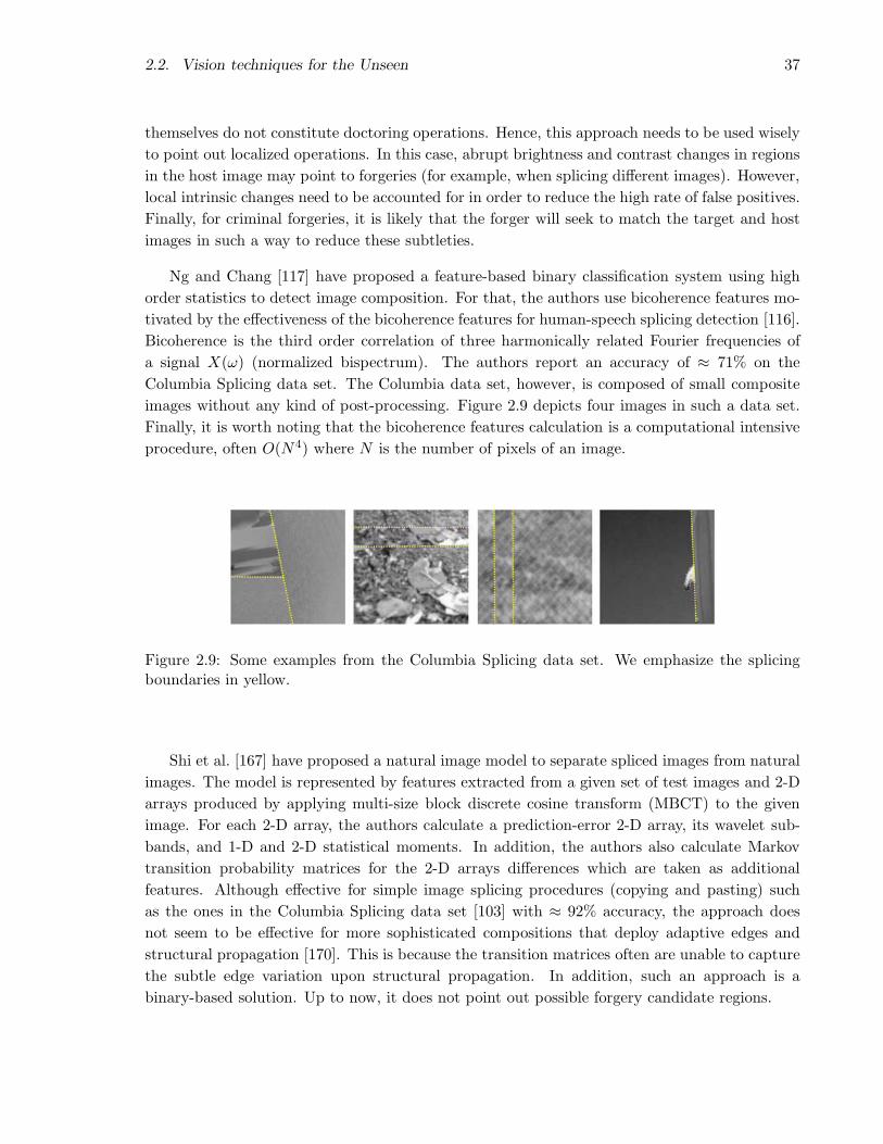
2.2. Vision techniques for the Unseen 37
themselves do not constitute doctoring operations. Hence, this approach needs to be used wisely
to point out localized operations. In this case, abrupt brightness and contrast changes in regions
in the host image may point to forgeries (for example, when splicing different images). However,
local intrinsic changes need to be accounted for in order to reduce the high rate of false positives.
Finally, for criminal forgeries, it is likely that the forger will seek to match the target and host
images in such a way to reduce these subtleties.
Ng and Chang [117] have proposed a feature-based binary classification system using high
order statistics to detect image composition. For that, the authors use bicoherence features mo-
tivated by the effectiveness of the bicoherence features for human-speech splicing detection [116].
Bicoherence is the third order correlation of three harmonically related Fourier frequencies of
a signal X(ω) (normalized bispectrum). The authors report an accuracy of ≈ 71% on the
Columbia Splicing data set. The Columbia data set, however, is composed of small composite
images without any kind of post-processing. Figure 2.9 depicts four images in such a data set.
Finally, it is worth noting that the bicoherence features calculation is a computational intensive
procedure, often O(N4) where N is the number of pixels of an image.
Figure 2.9: Some examples from the Columbia Splicing data set. We emphasize the splicingboundaries in yellow.
Shi et al. [167] have proposed a natural image model to separate spliced images from natural
images. The model is represented by features extracted from a given set of test images and 2-D
arrays produced by applying multi-size block discrete cosine transform (MBCT) to the given
image. For each 2-D array, the authors calculate a prediction-error 2-D array, its wavelet sub-
bands, and 1-D and 2-D statistical moments. In addition, the authors also calculate Markov
transition probability matrices for the 2-D arrays differences which are taken as additional
features. Although effective for simple image splicing procedures (copying and pasting) such
as the ones in the Columbia Splicing data set [103] with ≈ 92% accuracy, the approach does
not seem to be effective for more sophisticated compositions that deploy adaptive edges and
structural propagation [170]. This is because the transition matrices often are unable to capture
the subtle edge variation upon structural propagation. In addition, such an approach is a
binary-based solution. Up to now, it does not point out possible forgery candidate regions.

38 Chapter 2. Current Trends and Challenges in Digital Image Forensics
Inconsistencies in image features
When splicing two images to create a composite, one often needs to re-sample an image onto a
new sampling lattice using an interpolation technique (such as bi-cubic). Although impercepti-
ble, the re-sampling contains specific correlations that, when detected, may represent evidence of
tampering. Popescu and Farid [141] have described the form of these correlations, and proposed
an algorithm for detecting them in an image. The authors showed that the specific form of the
correlations can be determined by finding the neighborhood size, N , and the set of coefficients,
~α, that satisfy: ~ai =∑N
k=−N αk~ai+k in the equation
(
~ai −N∑
k=−N
αk~ai+k
)
· ~x = 0, (2.20)
where ~x is the signal, and ~ai is the ith row of the re-sampled matrix. The authors pointed out
that, in practice, neither the samples that are correlated, nor the specific form of the correlations
are known. Therefore, the authors employ an expectation maximization algorithm (EM) similar
to the one in Section 2.2.3 to simultaneously estimate a set of periodic samples correlated to
their neighbors and, an approximation form for these correlations. The authors assume that
each sample belongs to one of two models. The first model M1, corresponds to those samples yi
that are correlated to their neighbors and are generated according to the following model:
M1 : y1 =
−N∑
k
Nαkyi+k + n(i), (2.21)
where n(i) denote independently, and identically distributed samples drawn from a Gaussian
distribution with zero mean an unknown variance σ2. In the E-step, the probability that each
sample yi belonging to model M1 can be estimated through Bayes rule similarly to the Equa-
tion 2.9, Section 2.2.3, where yi replaces f(x, y). The probability of observing a sample yi know-
ing it was generated by M1 is calculated in the same way as in Equation 2.10, Section 2.2.3,
where yi replaces f(x, y). The authors claim that the generalization of their algorithm to color
images is fairly straightforward. The authors propose to analyze each color channel indepen-
dently. However, the authors do not show experiments for the performance of their algorithm
under such circumstances and to what extent such independence assumption is valid. Given
that demosaiced color images present high pixel correlation, such analysis would be valuable.
It is assumed that the probability of observing samples generated by the outlier model,
Pryi|yi ∈ M2, is uniformly distributed over the range of possible values of yi. Although, it
might seem a strong assumption, the authors do not go into more detail justifying the choice
of the uniform distribution for this particular problem. In the M-step, the specific form of the
correlations between samples is estimated minimizing a quadratic error function. It is important
to note that the re-sampling itself does not constitute tampering. One could just save space by
down-sampling every picture in a collection of pictures. However, when different correlations
are present in one image, there is a strong indication of image composition. The authors have
2.2. Vision techniques for the Unseen 39
reported very good results for high-quality images. As the image is compressed, specially under
JPEG 2000, the re-sampling correlates and hence tampering becomes harder to detect. It is
worth noting that it is also possible to perform a counter attack anticipating the tampering
detection and, therefore, destroying traces of re-sampling. Gloe et al. [58] presented a targeted
attack in which the pixel correlations are destroyed by small controlled geometric distortions.
The authors superimpose a random disturbance vector ~e to each individual pixel’s position. To
deal with possible jitter effects, the strength of distortion is adaptively modulated by the local
image content using simple edge detectors.
When creating a digital composite (for example, two people standing together), it is often dif-
ficult to match the lighting conditions from the individual photographs. Johnson and Farid [70]
have presented a solution that analyzes lighting inconsistencies to reveal traces of digital tamper-
ing. Standard approaches for estimating light source direction begin by making some simplifying
assumptions such as: (1) the surface is Lambertian (it reflects light isotropically); (2) it has a
constant reflectance value; (3) it is illuminated by a point light source infinitely far away; among
others. However, to estimate the lighting direction, standard solutions require knowledge of the
3-D surface normals from, at least, four distinct points on a surface with same reflectance, which
is hard to find from a single image and no objects of known geometry in the scene. The authors
have used a clever solution first proposed by [121] that estimates two components of the light
source direction from a single image. The authors also relax the constant reflectance assumption
by assuming that the reflectance for a local surface patch is constant. This requires the tech-
nique to estimate individual light source directions for each patch along a surface. Figure 2.10(a)
depicts an example where lighting inconsistencies can point out traces of tampering.
More recently, Johnson and Farid [71] have extended this solution to complex lighting en-
vironments by using spherical harmonics. Under the aforementioned simplifying assumptions,
an arbitrary lighting environment can be expressed as a non-negative function on the sphere,
L(~V ), ~V is a unit vector in Cartesian coordinates and the value of L(~V ) is the intensity of the
incident light along direction ~V . If the object being illuminated is convex, the irradiance (light
received) at any point on the surface is due to only lighting environment (no cast shadows or
inter-reflections).
It is worth noting, however, that even if the authors’ assumptions were true for an object,
which is rather limiting, they are virtually never true for a scene of interest given that a collection
of convex objects is no longer convex.
As a result, the irradiance, E( ~N), can be parametrized by the unit length surface normal~N and written as a convolution of the reflectance function on the surface, R(~V , ~N), with the
lighting environment L(~V ):
E( ~N ) =
∫
ΩL(~V )R(~V , ~N )dΩ (2.22)
where Ω represents the surface. For a Lambertian surface, the reflectance function is a clamped
cosine:
R(~V , ~N) = max(~V · ~N, 0). (2.23)

40 Chapter 2. Current Trends and Challenges in Digital Image Forensics
The convolution in Equation 2.22 can be simplified by expressing both the lighting envi-
ronment and the reflectance functions in terms of spherical harmonics. The main drawback of
such an approach is that in order to generate a good estimation of the lighting environment it
is necessary to learn the light behavior on a series of light probe images. A light probe image is
an omnidirectional, high dynamic range image that records the incident illumination conditions
at a particular point in space (see Figure 2.10(b)). Lighting environments can be captured by a
variety of methods such as photographing a mirror sphere or through panoramic photographic
techniques [36]. This is necessary to represent the lighting environment function L(~V ) that is
then integrated to result in the spherical harmonics representing the scene lighting.
(a) Composite example with lighting inconsis-tencies.
(b) Four light probes from different lighting environments.Credits to Paul Debevec and Dan Lemmon.
Figure 2.10: Lighting and forgeries.
More recently, Johnson and Farid [72] have also investigated lighting inconsistencies across
specular highlights on the eyes to identify composites of people. The position of a specular
highlight is determined by the relative positions of the light source, the reflective surface and
the viewer (or camera). According to the authors, specular highlights that appear on the eye
are a powerful cue as to the shape, color, and location of the light source(s). Inconsistencies
in these properties of the light can be used as telltales of tampering. It is worth noting that
specular highlights tend to be relatively small on the eye giving room to a more skilled forger
to manipulate them to conceal traces of tampering. To do so, shape, color, and location of the
highlight would have to be constructed so as to be globally consistent with the lighting in other
parts of the image.

2.2. Vision techniques for the Unseen 41
Acquisition inconsistencies
In the same way that we can use camera properties to point out the sensor that captured an
image, we also can use them as a digital X-ray for revealing forgeries [25].
Lin et al. [87] have presented an approach that explores camera response normality and
consistency functions to find tampering footprints. An image is tagged as doctored if the response
functions are abnormal or inconsistent to each other. The camera response function is a mapping
relationship between the pixel irradiance and the pixel value. For instance, suppose a pixel
is on an edge and the scene radiance changes across the edge and is constant on both sides
of the edge (Figure 2.11(a)). Therefore, the irradiance of the pixel on the edge should be a
linear combination of those of the pixels clear off the edges (Figure 2.11(b)). Due to nonlinear
response of the camera, the linear relationship breaks up among the read-out values of these
pixels (Figure 2.11(c)). The authors estimate the original linear relationship when calculating
the inverse camera response function [86]. Although effective in some situations, this approach
(a) (b) (c)
Figure 2.11: Camera Response Function Estimation. (a) R1 and R2 are two regions withconstant radiance. The third column images are a combination of R1 and R2. (b) The irradiancesof pixels in R1 map to the same point I1, in RGB color space. The same happens for pixelsin R2 which maps to I2. However, the colors of the pixels in the third column is the linearcombination of I1 and I2. (c) The camera response function f warps the line segment in (b)into a curve during read-out.
has several drawbacks. Namely, (1) to estimate the camera response function, the authors must
calculate an inverse camera response function which requires learning a Gaussian Mixture Model
from a database with several known camera response functions (DoRF) [87]. If the analyzed
image is a composite of regions from unknown cameras, the model is unable to point out an
estimation for the camera response function; (2) the approach requires the user to manually select
points on edges believed to be candidates for splicing; (3) the solution requires high contrast

42 Chapter 2. Current Trends and Challenges in Digital Image Forensics
images to perform accurate edge and camera normality estimations; (4) the approach might fail
if the spliced images are captured by the same camera and not synthesized along the edges of
an object; (5) Finally, it is likely the solution does not work with CMOS adaptive sensors that
dynamically calculate the camera response function to produce more pleasing pictures.
Chen et al. [25] have proposed to use inconsistencies in the photo-response non-uniformity
noise (c.f., Sec. 2.2.3) to detect traces of tampering. The method assumes that either the camera
that took the image or at least some other pristine images taken by the camera are available. The
algorithm starts by sliding a 128 × 128 block across the image and calculating the value of the
test statistics, pB, for each block B. The probability distribution function p(x|H0) of pB under
H0 is estimated by correlating the PRNU noise residuals from other cameras and is modeled as
a generalized Gaussian. For each block, the pdf p(x|H1) is obtained from a block correlation
predictor and is also modeled as a generalized Gaussian. For each block B, the authors perform
a Neyman-Pearson hypothesis testing by fixing the false alarm rate α and decide that B has been
tampered if pB < Th. The threshold Th is determined from the condition α =∫
Th p(x|H0)dx.
Structural inconsistencies
Some forgery detection approaches are devised specifically for a target. Popescu and Farid [140]
have discussed the effects of double quantization for JPEG images and presented a solution to
detect such effects. Double JPEG compression introduces specific artifacts not present in single
compressed images. The authors also note that evidence of double JPEG compression, however,
does not necessarily prove malicious tampering. For example, it is possible for a user to simply
re-save a high quality JPEG image with a lower quality. Figure 2.2.4 depicts an example of the
double quantization effect over a 1-d toy example signal x[t] normally distributed in the range
[0, 127].
(a) (b)
(c) (d)
Figure 2.12: The top row depicts histograms of single quantized signals with steps 2 (left) and3 (right). The bottom row depicts histograms of double quantized signals with steps 3 followedby 2 (left), and 2 followed by 3 (right). Note the periodic artifacts in the histograms of doublequantized signals. Credits to Alin Popescu.

2.2. Vision techniques for the Unseen 43
Inspired by the pioneering work of [140] regarding double quantization effects and their use
in forensics, He et al. [65] have proposed an approach to locate doctored parts in JPEG images
by examining the double quantization effect hidden among DCT coefficients. The idea is that
as long as a JPEG image contains both the doctored part and the pristine part, the discrete
cosine coefficient histograms of the pristine part will still have the double quantization effect
(DQ), because this part of the image is the same as that of the double compressed original
JPEG image. However, the histograms of a doctored part will not have the same DQ effects.
Some possible reasons for these observations are: (1) absence of the first JPEG compression in
the doctored part; (2) mismatch of the DCT grid of the doctored part with that of the pristine
part; or (3) composition of DCT blocks along the boundary may carry traces of the doctored
and pristine parts given that it is not likely that the doctored part exactly consists of 8 × 8
blocks. It is worth noting, however, that this solution will not work in some circumstances. For
instance, if the original image to contribute to the pristine part is not a JPEG image, the double
quantization effect of the pristine part cannot be detected. In addition, the compression levels
also affect the detection. Roughly speaking, the smaller the ratio of the second quantization
step with respect to the first one, the harder the detection of the DQ effects. Finally, if the
forger re-samples the grid of the DCT (shift the image one pixel), it is possible to destroy the
traces of the double quantization and generate a complete new quantization table.
2.2.5 Image and video hidden content detection/recovery
Steganography is the art of secret communication. Its purpose is to hide the presence of com-
munication — a very different goal than Cryptography, which aims to make communication
unintelligible for those that do not possess the correct access rights [6].
Applications of Steganography can include feature location (identification of subcomponents
within a data set), captioning, time-stamping, and tamper-proofing (demonstration that original
contents have not been altered). Unfortunately, not all applications are harmless, and there
are strong indications that Steganography has been used to spread child pornography on the
Internet [64, 113], and as an advanced communication tool for terrorists and drug-dealers [105,
106].
In response to such problems, the forensic analysis of such systems is paramount. We refer
to Forensic Steganalysis as the area related to the detection and recovery of hidden messages. In
this forensic scenario, we want to distinguish non-stego or cover objects, those that do not contain
a hidden message, and stego-objects, those that contain a hidden message with the additional
requirement of recovering its content as a possible proof basis for the court.
Steganography and Steganalysis have received a lot of attention around the world in the
past few years [149]. Some are interested in securing their communications through hiding the
very fact that they are exchanging information. On the other hand, others are interested in
detecting the existence of these communications — possibly because they might be related to
illegal activities. In the aftermath of 9/11 events, some researchers have suggested that Osama
Bin Laden and Al Qaeda used Steganography techniques to coordinate the World Trade Center
44 Chapter 2. Current Trends and Challenges in Digital Image Forensics
attacks. Almost six years later, nothing was proved [21,83,149,184]. However, since then, there
has been strong evidences that Steganography has been used as a private communication means
for drug-dealers and child pornographers in their illegal activities [64, 105, 106, 113]. Indeed,
according to the High Technology Crimes Annual Report [108,120], Steganography threats can
also appear in conjunction with dozens of other cyber-crimes such as: fraud and theft, terrorism,
computer cracking, online defamation, intellectual property offenses, and online harassment.
In the following sections, we present representative research with respect to the identification
and recovery of hidden messages in digital multimedia. When possible, we emphasize approaches
that can be used as an aid for criminal prosecution in a court of law. The fundamental goal
of Steganalysis is to reliably detect the existence of hidden messages in communications and,
indeed, most of the approaches in the literature have addressed only the detection problem.
However, for forensics purposes, we are interested in the higher level of analysis going one step
further and attempting to recover the hidden content.
We can model the detection of hidden messages in a cover medium as a classification problem.
In Steganalysis, we have two extreme scenarios: (1) Eve has only some level of suspicion that
Alice and Bob are covertly communicating; and (2) Eve may have some additional information
about Alice and Bob’s covert communications such as the algorithm they have used, for instance.
In the first case, we have a difficult forensic scenario where Eve would need to deploy a system
able to detect all forms of Steganography (Blind Steganalysis). In the latter case, Eve might
have additional information reducing her universe of possible hiding algorithms and cover media
(Targeted Steganalysis).
In general, steganographic algorithms rely on the replacement of some component of a digital
object with a pseudo-random secret message [6]. In digital images, common components used to
conceal data are: (1) the least significant bits (LSBs); (2) DCT coefficients in JPEG-compressed
images; and (3) areas with richness in details [32].
Figure 2.13 depicts a typical Steganography and Steganalysis scenario. When embedding
a message in an image, one can take several steps in order to avoid message detection such
as choosing an embedding key, compressing the message, and applying statistical profiling in
the message and the cover media in order to minimize the amount of changes. On the other
hand, in the Steganalysis scenario, we can try to point out the concealment whether making
statistical analysis on the input image, or on the image and on a set of positive and negative
training examples. If we have additional information, we can also use them in order to perform
a targeted attack. In the following, we present some approaches used to detect such activities
using either targeted or blind attacks.
Targeted Steganalysis
Some successful approaches for targeted Steganalysis proposed in the literature can estimate
the embedding ratio or even reveal the secret message with the knowledge of the steganographic
algorithm being very useful for forensics.
Basic LSB embedding can be reliably detected using the histogram attack as proposed

2.2. Vision techniques for the Unseen 45
Figure 2.13: Typical Steganography and Steganalysis scenario.
by [191]. Any possible LSB embedding procedure will change the contents of a selected number
of pixels and therefore will change the pixel value statistics in a local neighborhood.
An L-bit color channel can represent 2L possible values. If we split these values into 2L−1
pairs that only differ in the LSBs, we are considering all possible patterns of neighboring bits
for the LSBs. Each of these pairs are called pair of value (PoV) in the sequence [191].
When we use all the available LSB fields to hide a message in an image, the distribution of
odd and even values of a PoV will be the same as the 0/1 distribution of the message bits. The
idea of the statistical analysis is to compare the theoretically expected frequency distribution
of the PoVs with the real observed ones [191]. However, we do not have the original image and
thus the expected frequency. In the original image, the theoretically expected frequency is the
arithmetical mean of the two frequencies in a PoV. As we know, the embedding function only
affects the LSBs, so it does not affect the PoV’s distribution after an embedding. Therefore the
arithmetical mean remains the same in each PoV, and we can derive the expected frequency
through the arithmetic mean between the two frequencies in each PoV.
As presented in [143,191], we can apply the χ2 (chi squared-test) S over these PoVs to detect
hidden messages
S =
k∑
i=1
(f obsi − f exp
i )2
f expi
, (2.24)
where k is the number of analyzed PoVs, f obsi and f exp
i are the observed frequencies and the
expected frequencies respectively. A small value of S points out that the data follows the
expected distribution and we can conclude that the image was tweaked. We can measure the

46 Chapter 2. Current Trends and Challenges in Digital Image Forensics
statistical significance of S by calculating the p-value, which is the probability that a chi-square
distributed random variable with k − 1 degrees of freedom would attain a value larger than or
equal to S:
p(S) =1
2k−1
2 Γ(k−12 )
∫ ∞
Se
−x2 x
k−1
2−1dx. (2.25)
If the image does not have a hidden message, S is large and p(S) is small. In practice, we
calculate a threshold value Sth so that p(Sth) = α where α is the chosen significance level. The
main limitation with this approach is that it only detects sequential embeddings. For random
embeddings, we could apply this approach window-wise. However, in this case it is effective
only for large embeddings such as the ones that modify, at least, 50% of the available LSBs. For
small embeddings, there is a simple counter-attack that breaks down this detection technique.
For that, it is possible to learn the basic statistics about the image and to keep such statistics
when embedding the message. For instance, for each bit modified to one, another one is flipped
to zero. Indeed, as we shall show later, Outguess7 is one approach that uses such tricks when
performing embeddings in digital images.
Fridrich et al. [50] have presented RS analysis. It consists of the analysis of the LSB loss-
less embedding capacity in color and gray-scale images. The loss-less capacity reflects the fact
that the LSB plane — even though it looks random — is related to the other bit planes [50].
Modifications in the LSB plane can lead to statistically detectable artifacts in the other bit
planes of the image. The authors have reported good results (detection for message-sizes as
small as ≈ 2 − 5% on a limited set of images for the Steganography tools: Steganos, S-Tools,
Hide4PGP, among others8.
A similar approach was devised by [40] and is known as sample pair analysis. Such an
approach relies on the formation of some subsets of pixels whose cardinalities change with
LSB embedding, and such changes can be precisely quantified under the assumption that the
embedded bits form a random walk on the image. Consider the partitioning of the input image
in vectorized form V into pairs of pixels (u, v). Let P be the set of all pairs. Let us partition Pinto three disjoint sets X,Y , and Z, where
X = (u, v) ∈ P | (v is even and u < v) or (v is odd and u > v) Y = (u, v) ∈ P | (v is even and u > v) or (v is odd and u < v) Z = (u, v) ∈ P | (u = v) (2.26)
Furthermore, let us partition the subset Y into two subsets, W , and V , where V = Y \W , and
Y = (u, v) ∈ P | (u = 2k, v = 2k + 1) or (u = 2k + 1, v = 2k) (2.27)
The sets X,W,V, and Z are called primary sets and P = X ∪W ∪ V ∪ Z. When one embeds
content in an image, the LSB values are altered and therefore the cardinalities of the sets will
change accordingly. As we show in Figure 2.14, we have four possible cases π ∈ 00, 01, 10, 11.7http://www.outguess.org/8http://members.tripod.com/steganography/stego/software.html
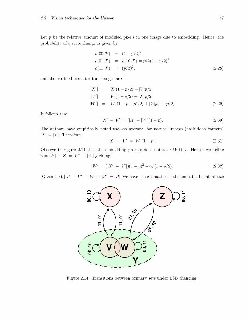
2.2. Vision techniques for the Unseen 47
Let p be the relative amount of modified pixels in one image due to embedding. Hence, the
probability of a state change is given by
ρ(00,P) = (1− p/2)2
ρ(01,P) = ρ(10,P) = p/2(1− p/2)2
ρ(11,P) = (p/2)2. (2.28)
and the cardinalities after the changes are
|X ′| = |X|(1 − p/2) + |V |p/2
|V ′| = |V |(1 − p/2) + |X|p/2
|W ′| = |W |(1− p + p2/2) + |Z|p(1− p/2) (2.29)
It follows that
|X ′| − |V ′| = (|X| − |V |)(1 − p). (2.30)
The authors have empirically noted the, on average, for natural images (no hidden content)
|X| = |Y |. Therefore,
|X ′| − |V ′| = |W |(1− p). (2.31)
Observe in Figure 2.14 that the embedding process does not alter W ∪ Z. Hence, we define
γ = |W |+ |Z| = |W ′|+ |Z ′| yielding
|W ′| = (|X ′| − |V ′|)(1 − p)2 + γp(1− p/2). (2.32)
Given that |X ′|+ |V ′|+ |W ′|+ |Z ′| = |P|, we have the estimation of the embedded content size
Figure 2.14: Transitions between primary sets under LSB changing.

48 Chapter 2. Current Trends and Challenges in Digital Image Forensics
0.5γp2 + (2|X ′| − |P|)p + |Y ′| − |X ′| = 0. (2.33)
This approach has been tested in [32] over three data sets summing up to 5,000 images. The
data sets comprise raw, compressed, and also scanned images. The approach is able to detect
messages as small as 5% of the available space for normal LSB embedding with no statistical
profiling.
Ker [80] has studied the statistical properties of the analysis of pairs and also proposed
an extension using weighted least squares [80]. Recently, Bohme [17] presented an extension
for JPEG covers. Several other approaches have been designed to detect targeted Steganalysis
specifically in the JPEG domain [49,56,133].
Shi et al. [166] have analyzed the gradient energy flipping rate during the embedding process.
The hypothesis is that the gradient energy varies consistently when the image is altered to conceal
data.
For most of the above techniques, the authors do not discuss possible counter-attacks to
their solutions. For instance, the sample pairs solution [40] and the RS analysis [50] rely on the
analysis of groups of modified and non-modified pixels. What happens if someone knows these
detection solutions and compensates for the group distribution for each modified pixel? Do the
solutions still work after such kind of embedding statistical profiling?
Blind Steganalysis
Most of the blind- and semi-blind detection approaches rely on supervised learning techniques.
The classifiers used in existing blind and semi-blind Steganalysis refer to virtually all categories
of classical classification such as regression, multi-variate regression, one class, two class, and
hyper-geometric classifications, among others.
Both in blind and semi-blind scenarios, the classifier is a mapping that depends on one or
more parameters that are determined through training and based on the desired tradeoff between
both type of errors (false alarm and false detection) that the classifier can make. Therefore,
Steganalysis begins with the appropriate choice of features to represent both the stego and
non-stego objects.
In the semi-blind scenario, we select a set of stego algorithms and train a classifier in the hope
that when analyzing an object concealing a message embedded with an unknown algorithm, the
detector will be able to generalize. On the other hand, in the complete blind scenario, we only
train a set of cover objects based on features we believe will be altered during the concealment
of data. In this case, we train one-class classifiers and use the trained model to detect outliers.
Some of the most common features used in the literature to feed classifiers are based on
wavelet image decompositions, image quality metrics, controlled perturbations, moment func-
tions, and histogram characteristic functions.
Lyu and Farid [95,96] have introduced a detection approach based on probability distribution
functions of image sub-bands coefficients. This work has become a basis for several others. The
motivation is that natural images have regularities that can be detected by high-order statistics
through quadrature mirror filter (QMF) decompositions [180].

2.2. Vision techniques for the Unseen 49
The QMF decomposition divides the image into multiple scales and orientations. We denotethe vertical, horizontal, and diagonal sub-bands in a given scale i = 1 . . . n as Vi(x, y),Hi(x, y), Di(x, y), respectively. Figure 2.15 depicts one image decomposition with three scales.The authors of [95,96] propose to detect hidden messages using two sets of statistics collected
Figure 2.15: Image sub-bands QMF decomposition.
throughout the multiple scales and orientations. The first set of statistics comprises mean,variance, skewness, and kurtosis. These statistics are unlikely to capture the strong correlationsthat exist across space, orientation, scale and color. Therefore, the authors calculate a secondset of statistics based on the errors in a linear predictor of coefficient magnitude. For the sake ofillustration, consider a vertical sub-band of a gray image at scale i, Vi(x, y). A linear predictorfor the magnitude of these coefficients in a subset of all possible spatial, orientation, and scaleneighbors is given by
|Vi(x, y)| = w1|Vi(x − 1, y)|+ w2|Vi(x + 1, y)|+ w3|Vi(x, y − 1)|+ w4|Vi(x, y + 1)|+ w5
∣
∣
∣Vi+1
(x
2,y
2
)∣
∣
∣+ w6|Di(x, y)|+ w7
∣
∣
∣Di+1
(x
2,y
2
)∣
∣
∣ , (2.34)
where | · | represents absolute value and wk are the weights. We can represent this linear
relationship in matrix form as ~V = Q~w, where the column vector ~w = (w1, . . . , w7)T , the
vector ~V contains the coefficient magnitudes of Vi(x, y) strung out into a column vector, and
the columns of the matrix Q contain the neighboring coefficient magnitudes as in Equation 2.34
also strung out into column vectors. The coefficients are determined through the minimization
of the quadratic error function
E(~w) = [~V −Q~w]2. (2.35)
This error is minimized through differentiation with respect to ~w. Setting the result equal to
zero, and solving for ~w, we have
~w = (QTQ)−1QT~V . (2.36)
Finally, the log error in the linear predictor is given by
~E = log2~V − log2(Q~w). (2.37)

50 Chapter 2. Current Trends and Challenges in Digital Image Forensics
It is from this error that the additional mean, variance, skewness, and kurtosis statistics are
collected. This process is repeated for each sub-band, and scale. From this set of statistics, the
authors train the detector with images with and without hidden messages.
Lyu and Farid [93, 97] have extended this set of features to color images and proposed an
one-class classifier with hyper-spheres representing cover objects. Outliers of this model are
tagged as stego objects. A similar procedure using Parzen-Windows was devised by [156] to
detect anomalies in stego systems.
Rocha and Goldenstein [147] have presented the Progressive Randomization meta-descriptor
for Steganalysis. The principle is that it captures the difference between image classes (with
and without hidden messages) by analyzing the statistical artifacts inserted during controlled
perturbation processes with increasing randomness.
Avcibas et al. [10] have presented a detection scheme based on image quality metrics (IQMs).
The motivation is that the embedding can be understood as an addition of noise to the image
therefore degrading its quality. They have used multivariate regression analysis. Avcibas et al. [8]
have introduced an approach that explores binary similarity measures within image bit planes.
The basic idea is that the correlation between the bit planes as well as the binary texture
characteristics within the bit planes differ between a stego image and a cover image.
Histogram characteristic functions and statistics of empirical co-occurrence matrices also
have been presented with relative success [26,49,168,193,194].
Despite of all the advances, one major drawback of the previous approaches is that most
of them are only able to point out whether or not a given image contains a hidden message.
Currently, with classifier-based blind or semi-blind approaches it is extremely difficult or even
impossible to identify portions of the image where a message is hidden and perform message
extraction or even only point out possible tools used in the embedding process. A second
drawback in this body of work is the lack of counter-analysis techniques to assess the viability
of the existing research. Outguess9 [142] and F5 [190] are two early examples of such works.
Outguess is a steganographic algorithm that relies on data specific handlers that extract
redundant bits and write them back after modification. For JPEG images, Outguess preserves
statistics based on frequency counts. As a result, statistical tests based on simple frequency
counts are unable to detect the presence of steganographic content [142]. Outguess uses a
generic iterator object to select which bits in the data should be modified. In addition, F5 was
proposed with the goal of providing high steganographic capacity without sacrificing security.
Instead of LSB flipping (traditional embedding approaches), the embedding operation in F5
preserves the shape of the DCT histogram. The embedding is performed according to a pseudo-
random path determined from a user pass-phrase. Later on, Fridrich et al. [52] have provided
a targeted attack that detects embedded messages using F5 algorithm throughout a process
called calibration. We estimate the original cover-object from the suspected stego-object. In
the case of JPEG images, for instance, this is possible because the quantized DCT coefficients
are robust to small distortions (the ones performed by some steganographic algorithms) [32].
9http://www.outguess.org/

2.2. Vision techniques for the Unseen 51
Fridrich et al.’s [52] approach is no longer as effective if we improve F5 with some sort of
statistical profiling preserving not only the DCT histogram shape but also compensating for the
modified coefficients.
Much more work of this sort is essential, given that this scenario looks like an arm’s race in
which Steganographers and Steganalyzers compete to produce better approaches in a techno-
logical escalation.
In the Stegi@Work section, we present a common framework that allows us to combine most
of the state of the art solutions in a compact and efficient way toward the objective of recovering
the hidden content.
Some other flaws related to the classifier-based blind or semi-blind approaches are
• The choice of proper features to train the classifier upon is a key step. There is no
systematic rule for feature selection. It is mostly a heuristic, trial and error method [24].
• Some classifiers have several parameters that have to be chosen (type of kernels, learning
rate, training conditions) making the process a hard task [24].
• To our knowledge, a standard reference set has yet to emerge in the Steganalysis field
to allow fair comparison across different approaches. One step in that direction is the
work of [154] which presents two controlled data sets to test hidden message detection
approaches and the work of [79] which presents a new benchmark for binary steganalysis
methods.
Stegi@Work
What is needed for today’s forensics applications is a scalable framework that is able to process a
large volume of images (the sheer volume of images on sites such as Flickr and Picasa is testament
to this). As we have repeatedly seen throughout this paper, individual techniques for forensic
analysis have been developed for specific tools, image characteristics, and imaging hardware,
with results presented in the limited capacity of each individual work’s focus. If a high capacity
framework for digital image forensics was available, the forensic tools presented in this paper
could be deployed in a common way, allowing the application of many tools against a candidate
image, with the fusion of results giving a high-confidence answer as to whether an image contains
steganographic content, is a forgery, or has been produced by a particular imaging system. In
our own work in the “Vision of the Unseen,” we have focused on the development of a cross-
platform distributed framework specifically for Steganalysis, embodying the above ideas, that
we call Stegi@Work. In this section, we will summarize the overall architecture and capabilities
of the Stegi@Work framework as an example of what a distributed forensics framework should
encompass.
Stegi@Work, at the highest architectural level (details in Figure 2.16), consists of three
entities. A requester client issues jobs for the system to process. Each job consists of a file that
does or does not contain steganographic content. This file is transmitted to the Stegi server,
which in turn, dispatches the job’s processing to the worker clients. Much like other distributed
52 Chapter 2. Current Trends and Challenges in Digital Image Forensics
computing frameworks such as Seti@home10 and Folding@home11, worker clients can be ordinary
workstations on a network with CPU cycles to spare. The Stegi server collects the results for
each job, and performs fusion over the set of results, to come to a final conclusion about the
status of the file in question. Each network entity may be connected via a LAN, or logically
separated by firewalls in a WAN, facilitating the use of worker clients or requestor clients on
a secure or classified network, while maintaining presence on an insecure network, such as the
Internet. The Stegi server exists as the common point of contact for both.
The specifics of job communication (details in Figure 2.17), include the specific definitions
for each job packet transmitted between network entities. Between the requester client and
the Stegi server, both job request and job results packets are exchanged. In a job request, the
file in question is transmitted to the server, along with optional tool selection and response
requests. If these are not specified, the server can choose them automatically based on the
type of the submitted file, as well as a defined site policy. The server receives a detailed report
packet from each worker client, including the results of all of the tools applied against a file, as
well as additional details about the job, such as execution time. Additional status packets are
transmitted between all network entities, including server status to a worker client, notifying
it that a job (with the file and appropriate tools) is ready, worker client status to the server,
indicating the current state of a job, and server status to a worker client indicating what should
be known about a job that is in the system.
The Stegi@Work architecture provides tool support for each worker client in the form of a
wrapper API around the tool for each native platform. This API defines process handling, pro-
cess status, and control signaling, allowing the Stegi server full control over each process on each
worker client. The current system as implemented supports wrappers written in C/C++, Java,
and Matlab, thus supporting a wide range of tools on multiple platforms. Network communica-
tion between each native tool on the worker client and the Stegi@Work system is defined via a
set of XML messages. We have created wrappers for the popular analysis tools stegdetect12 and
Digital Invisible Ink Toolkit13, as well as a custom tool supporting signature-based detection,
as well as the statistical χ2 test.
In order for high portability, allowing for many worker clients, the Stegi@Work framework
has been implemented in Java, with tool support, as mentioned above, in a variety of different
languages. This is accomplished through the use of Java Native Interface14 (JNI), with Win32
and Linux calls currently supported. The Stegi@Work server is built on top of JBOSS15, with
an Enterprise Java Beans16 (EJB) 3.0 object model for all network entities. GUI level dialogues
are available for system control at each entity throughout the framework.
The actual use cases for a system like Stegi@Work extend beyond large-scale forensics for
10http://setiathome.berkeley.edu/11http://folding.stanford.edu/12http://www.outguess.org/detection.php13http://diit.sourceforge.net/14http://swik.net/JNI+Tutorial15http://www.jboss.org/16http://www.conceptgo.com/gsejb/index.html
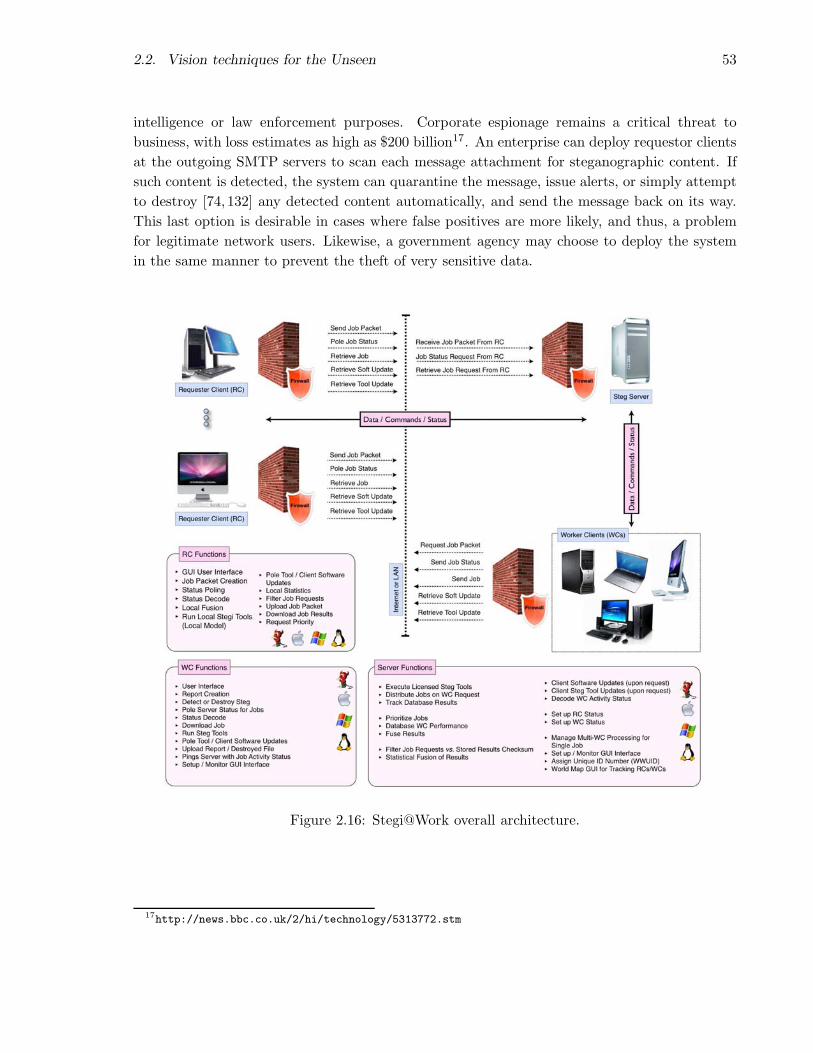
2.2. Vision techniques for the Unseen 53
intelligence or law enforcement purposes. Corporate espionage remains a critical threat to
business, with loss estimates as high as $200 billion17. An enterprise can deploy requestor clients
at the outgoing SMTP servers to scan each message attachment for steganographic content. If
such content is detected, the system can quarantine the message, issue alerts, or simply attempt
to destroy [74, 132] any detected content automatically, and send the message back on its way.
This last option is desirable in cases where false positives are more likely, and thus, a problem
for legitimate network users. Likewise, a government agency may choose to deploy the system
in the same manner to prevent the theft of very sensitive data.
Figure 2.16: Stegi@Work overall architecture.
17http://news.bbc.co.uk/2/hi/technology/5313772.stm

54 Chapter 2. Current Trends and Challenges in Digital Image Forensics
Figure 2.17: Stegi@Work communications architecture.
2.3 Conclusions
A remarkable demand for image-based forensics has emerged in recent years in response to a
growing need for investigative tools for a diverse set of needs. From the law enforcement com-
munity’s perspective, image based analysis is crucial for the investigation of many crimes, most
notably child pornography. Yet, crime that utilizes images is not limited to just pornography,
with entities as diverse as Colombian drug cartels taking advantage of steganography to mask
their activities. From the intelligence community’s perspective, the ability to scan large amounts
of secret and public data for tampering and hidden content is of interest for strategic national
security. As the case of the Iranian missiles has shown, state based actors are just as willing to
abuse image processing as common criminals.
But the obvious crimes are not necessarily the most damaging. The digital world presents
its denizens with a staggering number of images of dubious authenticity. Disinformation via the
media has been prevalent throughout the last century, with doctored images routinely being used
for political propaganda. But now, with the near universal accessibility of digital publishing,
disinformation has spread to commercial advertising, news media, and the work of malicious
pranksters. Is it at all possible to determine whether an image is authentic or not? If we cannot
determine the authenticity, what are we to believe about the information the image represents?
Digital Image and Video Forensics research aims at uncovering and analyzing the underlying
facts about an image/video. Its main objectives comprise: tampering detection (cloning, healing,
retouching, splicing), hidden messages detection/recovery, and source identification with no
prior measurement or registration of the image (the availability of the original reference image
or video). In this paper, we have taken a look at many individual algorithms and techniques
designed for very specific detection goals. However, the specific nature of the entire body of
digital image and video forensics work is its main limitation at this point in time. How is an
investigator able to choose the correct method for an image at hand? Moreover, the shear

2.4. Acknowledgments 55
magnitude of images that proliferate throughout the Internet poses a serious challenge for large-
scale hidden content detection or authenticity verification.
In response to this challenge, we make several recommendations. First, work on decision level
and temporal fusion serves as an excellent basis for operational systems. Combining information
from many algorithms and techniques yields more accurate results — especially when we do not
know precisely what we are looking for. Second, the need for large distributed (or clustered)
systems for parallel evaluation fills an important role for national and corporate security. Our
Stegi@Work system is an example of this. Third, the evaluation of existing and new algorithms
must be improved. The analysis of detection results in nearly all papers surveyed lacks the rigor
found in other areas of digital image processing and computer vision, making the assessment of
their utility difficult. More troubling, in our paper, only a few papers on counter-forensics for
image based forensics were found, leading us to question the robustness of much of the work
presented here to a clever manipulator. Finally, for forgery detection and steganalysis, more
powerful algorithms are needed to detect specifics about manipulations found in images, not
just that an image has been tampered with. Despite these shortcoming, the advancement of the
state of the art will continue to improve our Vision of the Unseen.
2.4 Acknowledgments
We would like to thank the financial support of Fapesp (Contracts 05/58103-3 and 07/52015-0),
CNPq (Contracts 309254/2007-8 and 551007/2007-9), and United States Air Force STTR (Con-
tract FA9550-05-C-0172).


Esteganografia e Esteganalise nos
Meios Digitais
No Capıtulo 3, discutimos algumas das principais tecnicas para o mascaramento digital de
informacoes e para a deteccao de mensagens escondidas em imagens.
Mostramos que uma das areas que tem recebido muita atencao recentemente e a estegano-
grafia. Esta e a arte de mascarar informacoes e evitar a sua deteccao. Esteganografia deriva
do grego, onde estegano = “esconder, mascarar” e grafia = “escrita”. Logo, esteganografia e a
arte da escrita encoberta.
Aplicacoes de esteganografia incluem identificacao de componentes dentro de um subconjunto
de dados, legendagem (captioning), rastreamento de documentos e certificacao digital (time-
stamping) e demonstracao de que um conteudo original nao foi alterado (tamper-proofing).
Entretanto, ha indıcios recentes de que a esteganografia tem sido utilizada para divulgar imagens
de pornografia infantil na internet [64,113].
Desta forma, e importante desenvolvermos algoritmos para detectar a existencia de mensa-
gens escondidas. Neste contexto, aparece a esteganalise digital, que se refere ao conjunto de
tecnicas que sao desenvolvidas para distinguir entre objetos que possuem conteudo escondido
(estego-objetos) daqueles que nao o possuem (nao-estego).
Finalmente, apresentamos as principais tendencias relacionadas a Esteganografia e Este-
ganalise digitais bem como algumas oportunidades de pesquisa.
O trabalho apresentado no Capıtulo 3 e o resultado de nosso artigo [149] na Revista de
Informatica Teorica e Aplicada (RITA).
57


Chapter 3
Steganography and Steganalysis in
Digital Multimedia: Hype or
Hallelujah?
Abstract
In this paper, we introduce the basic theory behind Steganography and Steganalysis, and present
some recent algorithms and developments of these fields. We show how the existing techniques
used nowadays are related to Image Processing and Computer Vision, point out several trendy
applications of Steganography and Steganalysis, and list a few great research opportunities just
waiting to be addressed.
3.1 Introduction
De artificio sine secreti latentis suspicione scribendi!1. (David Kahn)
More than just a science, Steganography is the art of secret communication. Its purpose is
to hide the presence of communication, a very different goal than Cryptography, that aims to
make communication unintelligible for those that do not possess the correct access rights [6].
Applications of Steganography can include feature location (identification of subcomponents
within a data set), captioning, time-stamping, and tamper-proofing (demonstration that original
contents have not been altered). Unfortunately, not all applications are harmless, and there are
strong indications that Steganography has been used to spread child pornography pictures on
the internet [64,113].
In this way, it is important to study and develop algorithms to detect the existence of hidden
messages. Digital Steganalysis is the body of techniques that attempts to distinguish between
1The effort of secret communication without raising suspicions.
59

60 Chapter 3. Steganography and Steganalysis in Digital Multimedia: Hype or Hallelujah?
non-stego or cover objects, those that do not contain a hidden message, and stego-objects, those
that contain a hidden message.
Steganography and Steganalysis have received a lot of attention around the world in the
past few years. Some are interested in securing their communications through hiding the very
own fact that they are exchanging information. On the other hand, others are interested in
detecting the existence of these communications — possibly because they might be related to
illegal activities.
In this paper, we introduce the basic theory behind Steganography and Steganalysis, and
present some recent algorithms and developments of these fields. We show how the existing
techniques used nowadays are related to Image Processing and Computer Vision, point out
several trendy applications of Steganography and Steganalysis, and list a few great research
opportunities just waiting to be addressed.
The remainder of this paper is organized as follows. In Section 3.2, we introduce the main
concepts of Steganography and Steganalysis. Then, we present historical remarks and social
impacts in Sections 3.3 and 3.4, respectively. In Section 3.5, we discuss information hiding for
scientific and commercial applications. In Sections 3.6 and 3.7, we point out the main techniques
of Steganography and Steganalysis. In Section 3.8, we present common-available information
hiding tools and software. Finally, in Sections 3.9 and 3.10, we point out open research topics
and conclusions.
3.2 Terminology
According to the general model of Information Hiding : embedded data is the message we want
to send secretly. Often, we hide the embedded data in an innocuous medium, called cover
message. There are many kinds of cover messages such as cover text, when we use text to hide
a message; or cover image, when we use an image to hide a message. The embedding process
produces a stego object which contains the hidden message. We can use a stego key to control
the embedding process, so we can also restrict detection and/or recovery of the embedded data
to other parties with the appropriate permissions to access this data.
Figure 3.1 shows the process of hiding a message in an image. First we choose the data we
want to hide. Further, we use a selected key to hide the message in a previously selected cover
image which produces the stego image.
When designing information hiding techniques, we have to consider three competing aspects:
capacity, security, and robustness [144]. Capacity refers to the amount of information we can
embed in a cover object. Security relates to an eavesdropper’s inability to detect the hidden
information. Robustness refers to the amount of modification the stego-object can withstand
before an adversary can destroy the information [144]. Steganography strives for high security
and capacity. Hence, a successful attack to the Steganography consists of the detection of the
hidden content. On the other hand, in some applications, such as watermarking, there is the
additional requirement of robustness. In these cases, a successful attack consists in the detection
and removal of the copyright marking.

3.2. Terminology 61
Message to be hidden
The cover medium
to be used
The produced stego image
Figure 3.1: A data hiding example.
Figure 3.2 presents the Information Hiding hierarchy [135]. Covert channels consist of the
use of a secret and secure channel for communication purposes (e.g., military covert channels).
Steganography is the art, and science, of hiding the information to avoid its detection. It derives
from the Greek steganos ∼ “hide, embed” and graph ∼ “writing”.
We classify Steganography as technical and linguistic. When we use physical means to conceal
the information, such as invisible inks or micro-dots, we are using technical Steganography. On
the other hand, if we use only “linguistic” properties of the cover object, such as changes in
image pixels or letter positions, in a cover text we are using linguistic Steganography.
Information Hiding
Covert channels Steganography
Linguistic Technical
Anonymity Copyright marking
Robust watermarking Fragile watermarking
Fingerprinting Watermarking
Perceptible Imperceptible
Figure 3.2: Information Hiding hierarchy.
Copyright marking refers to the group of techniques devised to identify the ownership of
intellectual property over information. It can be fragile, when any modification on the media
leads to the loss of the marking; or robust, when the marking is robust to some destructive

62 Chapter 3. Steganography and Steganalysis in Digital Multimedia: Hype or Hallelujah?
attacks.
Robust copyright marking can be of two types: fingerprinting and watermarking. Finger-
printing hides an unique identifier of the customer who originally acquired the information,
recording in the media its ownership. If the copyright owner finds the document in the posses-
sion of an unwanted party, she can use the fingerprint information to identify, and prosecute,
the customer who violated the license agreement.
Unlike fingerprints, watermarks identify the copyright owner of the document, not the iden-
tity of the customer. Furthermore, we can classify watermarking according to its visibility to
the naked eye as perceptible or imperceptible.
In short, fingerprints are used to identify violators of the license agreement, while watermarks
help with prosecuting those who have an illegal copy of a digital document [131,135].
Anonymity is the body of techniques devised to surf the Web secretly. This is done using
sites like Anonymizer2 or remailers (blind e-mailing services).
3.3 Historical remarks
Throughout history, people always have aspired to more privacy and security for their commu-
nications [77, 122]. One of the first documents describing Steganography comes from Histories
by Herodotus, the Father of History. In this work, Herodotus gives us several cases of such
activities. A man named Harpagus killed a hare and hid a message in its belly. Then, he sent
the hare with a messenger who pretended to be a hunter [122].
In order to convince his allies that it was time to begin a revolt against Medes and the
Persians, Histaieus shaved the head of his most trusted slave, tattooed the message on his head
and waited until his hair grew back. After that, he sent him along with the instruction to shave
his head only in the presence of his allies.
Another technique was the use of tablets covered by wax, first used by Demeratus, a Greek
who wanted to report from the Persian court back to his friends in Greece that Xerxes, the Great,
was about to invade them. The normal use of wax tablets consisted in writing the text in the
wax over the wood. Demeratus, however, decided to melt the wax, write the message directly
to the wood, and then put a new layer of wax on the wood in such a way that the message
was not visible anymore. With this ingenious action, the tablets were sent as apparently blank
tablets to Greece. This worked for a while, until a woman named Gorgo guessed that maybe
the wax was hiding something. She removed the wax and became the first woman cryptanalyst
in History.
During the Renaissance, the Harpagus’ hare technique was “improved” by Giovanni Porta,
one of the greatest cryptologists of his time, who proposed feeding a message to a dog and then
killing the dog [77].
Drawings were also used to conceal information. It is a simple matter to hide information
by varying the length of a line, shadings, or other elements of the picture. Nowadays, we have
2www.anonymizer.com

3.4. Social impacts 63
proof that great artists, such as Leonardo Da Vinci, Michelangelo, and Rafael, have used their
drawings to conceal information [77]. However, we still do not have any means to identify the
real contents, or even intention, of these messages.
Sympathetic inks were a widespread technique. Who has not heard about lemon-based ink
during childhood? With this type of ink, it is possible to write an innocent letter having a very
different message written between its lines.
Science has developed new chemical substances that, combined with other substances, cause
a reaction that makes the result visible. One of them is gallotanic acid, made from gall nuts,
that becomes visible when coming in contact with copper sulfate [137].
With the continuous improvement of lenses, photo cameras, and films, people were able to
reduce the size of a photo down to the size of a printed period [77, 122]. One such example
is micro-dot technology, developed by the Germans during the Second World War, referred to
as the “enemy’s masterpiece of espionage” by the FBI’s director J. Edgar Hoover. Micro-dots
are photographs the size of a printed period that have the clarity of standard-sized typewritten
pages. Generally, micro-dots were not hidden, nor encrypted messages. They were just so
small as to not draw attention to themselves. The micro-dots allowed the transmission of large
amounts of data (e.g., texts, drawings, and photographs) during the war.
There are also other forms of hidden communications, like null ciphers. Using such tech-
niques, the real message is “camouflaged” in an innocuous message. The messages are very hard
to construct and usually look like strange text. This strangeness factor can be reduced if the
constructor has enough space and time. A famous case of a null cipher is the book Hypterono-
machia Poliphili of 1499. A Catholic priest named Colona decided to declare his love to a young
lady named Polya by putting the message “Father Colona Passionately loves Polia” in the first
letter of each chapter of his book.
3.4 Social impacts
Science and technology changed the way we lived in the 20th century. However, this progress
is not without risk. Evolution may have a high social impact, and digital Steganography is no
different.
Over the past few years, Steganography has received a lot of attention. Since September 11th,
2001, some researchers have suggested that Osama Bin Laden and Al Qaeda used Steganography
techniques to coordinate the World Trade Center attacks. Several years later, nothing was
proved [21,83,147,184]. However, since then, Steganography has been a hype.
As a matter of fact, it is important to differentiate what is merely a suspicion from what is
real — the hype or the hallelujah. There are many legal uses for Steganography and Steganaly-
sis, as we show in Section 3.5. For instance, we can employ Steganography to create smart data
structures and robust watermarking to track and authenticate documents, to communicate pri-
vately, to manage digital elections and electronic money, to produce advanced medical imagery,
and to devise modern transit radar systems. Unfortunately, there are also illegal uses of these
techniques. According to the High Technology Crimes Annual Report [108,120], Steganography

64 Chapter 3. Steganography and Steganalysis in Digital Multimedia: Hype or Hallelujah?
and Steganalysis can be used in conjunction with dozens of other cyber-crimes such as: fraud
and theft, child pornography, terrorism, hacking, online defamation, intellectual property of-
fenses, and online harassment. There are strong indications that Steganography has been used
to spread child pornography pictures on the internet [64,113].
In this work, we present some possible techniques and legal applications of Steganography
and Steganalysis. Of course, the correct use of the information therein is all part of the reader’s
responsibility.
3.5 Scientific and commercial applications
In this section, we show that there are many applications for Information Hiding.
• Advanced data structures. We can devise data structures to conceal unplanned infor-
mation without breaking compatibility with old software. For instance, if we need extra
information about photos, we can put it in the photos themselves. The information will
travel with the photos, but it will not disturb old software that does not know of its exis-
tence. Furthermore, we can devise advanced data structures that enable us to use small
pieces of our hard disks to secretly conceal important information [63,125].
• Medical imagery. Hospitals and clinical doctors can put together patient’s exams, im-
agery, and their information. When a doctor analyzes a radiological exam, the patient’s
information is embedded in the image, reducing the possibility of wrong diagnosis and/or
fraud. Medical-image steganography requires extreme care when embedding additional
data within the medical images: the additional information must not affect the image
quality [85,157].
• Strong watermarks. Creators of digital content are always devising techniques to de-
scribe the restrictions they place on their content. These technique can be as simple as
the message “Copyright 2007 by Someone” [188], as complex as the digital rights man-
agement system (DRM) devised by Apple Inc. in its iTunes store’s contents [175], or the
watermarks in the contents of the Vatican Library [110].
• Military agencies. Militaries’ actions can be based on hidden and protected communica-
tions. Even with crypto-graphed content, the detection of a signal in a modern battlefield
can lead to the rapid identification and attack of the involved parties in the communi-
cation. For this reason, military-grade equipment uses modulation and spread spectrum
techniques in its communications [188].
• Intelligence agencies. Justice and Intelligence agencies are interested in studying these
technologies, and identifying their weaknesses to be able to detect and track hidden mes-
sages [64,109,113].

3.6. Steganography 65
• Document tracking tools. We can use hidden information to identify the legitimate
owner of a document. If the document is leaked, or distributed to unauthorized parties,
we can track it back to the rightful owner and perhaps discover which party has broken
the license distribution agreement [188].
• Document authentication. Hidden information bundled into a document can contain
a digital signature that certifies its authenticity [188].
• General communication. People are interested in these techniques to provide more
security in their daily communications [184, 188]. Many governments continue to see the
internet, corporations, and electronic conversations as an opportunity for surveillance [164].
• Digital elections and electronic money. Digital elections and electronic money are
based on secret and anonymous communications techniques [135,188].
• Radar systems. Modern transit radar systems can integrate information collected in a
radar base station, avoiding the need to send separate text and pictures to the receiver’s
base stations.
• Remote sensing. Remote sensing can put together vector maps and digital imagery of a
site, further improving the analysis of cultivated areas, including urban and natural sites,
among others.
3.6 Steganography
In this section, we present some of the most common techniques used to embed messages in
digital images. We choose digital images as cover objects because they are more related to
Computer Vision and Image Processing. However, these techniques can be extended to other
types of digital media as cover objects, such as text, video, and audio files.
In general, steganographic algorithms rely on the replacement of some noise component of
a digital object with a pseudo-random secret message [6]. In digital images, the most common
noise component is the least significant bits (LSBs). To the human eye, changes in the value
of the LSB are imperceptible, thus making it an ideal place for hiding information without any
perceptual change in the cover object.
The original LSB information may have statistical properties, so changing some of them
could result in the loss of those properties. Thus, we have to embed the message mimicking the
characteristics of the cover bits’ [137]. One possibility is to use a selection method in which we
generate a large number of cover messages in the same way, and we choose the one having the
secret embedded in it. However, this method is computationally expensive and only allows small
embeddings. Another possibility is to use a constructive method. In this approach, we build a
mimic function that also simulates characteristics of the cover bits noise.
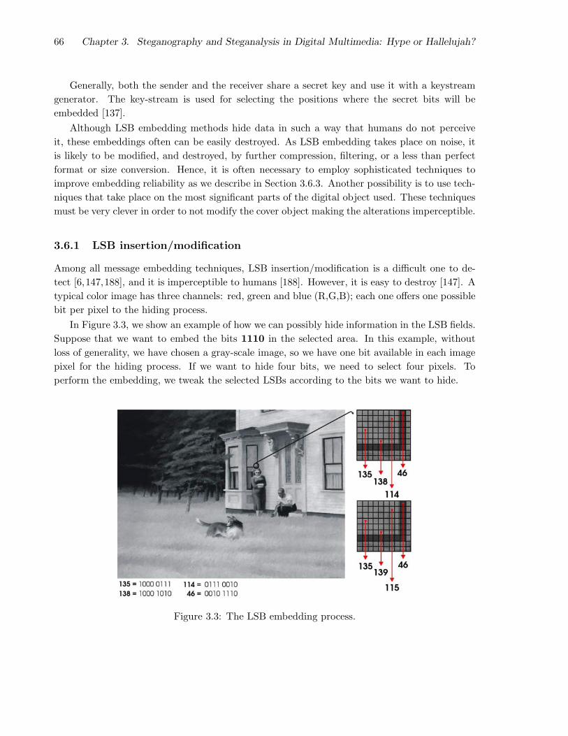
66 Chapter 3. Steganography and Steganalysis in Digital Multimedia: Hype or Hallelujah?
Generally, both the sender and the receiver share a secret key and use it with a keystream
generator. The key-stream is used for selecting the positions where the secret bits will be
embedded [137].
Although LSB embedding methods hide data in such a way that humans do not perceive
it, these embeddings often can be easily destroyed. As LSB embedding takes place on noise, it
is likely to be modified, and destroyed, by further compression, filtering, or a less than perfect
format or size conversion. Hence, it is often necessary to employ sophisticated techniques to
improve embedding reliability as we describe in Section 3.6.3. Another possibility is to use tech-
niques that take place on the most significant parts of the digital object used. These techniques
must be very clever in order to not modify the cover object making the alterations imperceptible.
3.6.1 LSB insertion/modification
Among all message embedding techniques, LSB insertion/modification is a difficult one to de-
tect [6,147,188], and it is imperceptible to humans [188]. However, it is easy to destroy [147]. A
typical color image has three channels: red, green and blue (R,G,B); each one offers one possible
bit per pixel to the hiding process.
In Figure 3.3, we show an example of how we can possibly hide information in the LSB fields.
Suppose that we want to embed the bits 1110 in the selected area. In this example, without
loss of generality, we have chosen a gray-scale image, so we have one bit available in each image
pixel for the hiding process. If we want to hide four bits, we need to select four pixels. To
perform the embedding, we tweak the selected LSBs according to the bits we want to hide.
Figure 3.3: The LSB embedding process.

3.6. Steganography 67
3.6.2 FFTs and DCTs
A very effective way of hiding data in digital images is to use a Direct Cosine Transform (DCT),
or a Fast Fourier Transform (FFT), to hide the information in the frequency domain. The DCT
algorithm is one of the main components of the JPEG compression technique [60]. In general,
DCT and FFT work as follows:
1. Split the image into 8× 8 blocks.
2. Transform each block via a DCT/FFT. This outputs a multi-dimensional array of 64
coefficients.
3. Use a quantizer to round each of these coefficients. This is essentially the compression
stage and it is where data is lost. Small unimportant coefficients are rounded to 0 while
larger ones lose some of their precision.
4. At this stage you should have an array of streamlined coefficients, which are further com-
pressed via a Huffman encoding scheme or something similar.
5. To decompress, use the inverse DCT/FFT.
The hiding process using a DCT/FFT is useful because anyone that looks at pixel values of
the image would be unaware that anything is different [188].
Least significant coefficients.
It is possible to use LSB of the quantized DCT/FFT coefficients as redundant bits, and embed
the hidden message there. The modification of a single DCT/FFT coefficient affects all 64 image
pixels in the block [144]. Two of the simpler frequency-hiding algorithms are JSteg [179] and
Outguess [142].
JSteg, Algorithm 2, sequentially replaces the least significant bit of DCT, or FFT, coefficients
with the message’s data. The algorithm does not use a shared key, hence, anyone who knows
the algorithm can recover the message’s hidden bits.
On the other hand, Outguess, Algorithm 3, is an improvement over JSteg, because it uses a
pseudo-random number generator (PRNG) and a shared key as the PRNG’s seed to choose the
coefficients to be used.
Block tweaking.
It is possible to hide data during the quantization stage [188]. If we want to encode the bit value
0 in a specific 8× 8 square of pixels, we can do this by making sure that all the coefficients are
even in such a block, for example by tweaking them. In a similar approach, bit value 1 can be
stored by tweaking the coefficients so that they are odd.
With the block tweaking technique, a large image can store some data that is quite difficult
to destroy when compared to the LSB method. Although this is a very simple method and
works well in keeping down distortions, it is vulnerable to noise [6, 188].

68 Chapter 3. Steganography and Steganalysis in Digital Multimedia: Hype or Hallelujah?
Algorithm 2 JSteg general algorithm
Require: message M , cover image I;1: procedure JSteg(M, I)2: while M 6= NULL do3: get next DCT coefficient from I;4: if DCT 6= 0 and DCT 6= 1 then ⊲ We only change non-0/1 coefficients5: b ← next bit from M ;6: replace DCT LSB with message bit b;7: M ←M − b;8: end if9: Insert DCT into stego image S;
10: end whilereturn S;
11: end procedure
Algorithm 3 Outguess general algorithm
Require: message M , cover image I, shared key k;1: procedure Outguess(M, I, k)2: Initialize PRNG with the shared key k3: while M 6= NULL do4: get pseudo-random DCT coefficient from I;5: if DCT 6= 0 and DCT 6= 1 then ⊲ We only change non-0/1 coefficients6: b ← next bit from M ;7: replace DCT LSB with message bit b;8: M ←M − b;9: end if
10: Insert DCT into stego image S;11: end while
return S;12: end procedure

3.6. Steganography 69
Coefficient selection.
This technique consists of the selection of the k largest DCT or FFT coefficients γ1 . . . γk and
modify them according to a function f that also takes into account a measure α of the required
strength of the embedding process. Larger values of α are more resistant to error, but they also
introduce more distortions.
The selection of the coefficients can be based on visual significance (e.g., given by zigzag
ordering [188]). The factors α and k are user-dependent. The function f(·) can be
f(γ′i) = γi + αbi, (3.1)
where bi is a bit we want to embed in the coefficient γi.
Wavelets.
DCT/FFT transformations are not so effective at higher-compression levels. In such scenarios,
we can use wavelet transformations instead of DCT/FFTs to improve robustness and reliability.
Wavelet-based techniques work by taking many wavelets to encode a whole image. They
allow images to be compressed by storing the high and low frequency details separately in the
image. We can use the low frequencies to compress the data, and use a quantization step to
compress even more. Information hiding techniques using wavelets are similar to the ones with
DCT/FFT [188].
3.6.3 How to improve security
Robust Steganography systems must observe the Kerckhoffs’ Principle [160] in Cryptography,
which holds that a cryptographic system’s security should rely solely on the key material. Fur-
thermore, to remain undetected, the unmodified cover medium used in the hiding process must
be kept secret or destroyed. If it is exposed, a comparison between the cover and stego media
immediately reveals the changes.
Further procedures to improve security in the hiding process are:
• Cryptography. Steganography supplements Cryptography, it does not replace it. If
a hidden message is encrypted, it must also be decrypted if discovered, which provides
another layer of protection [73].
• Statistical profiling. Data embedding alters statistical properties of the cover medium.
To overcome such alterations, the embedding procedure can learn the statistics about the
cover medium in order to minimize the amount of changes. For instance, for each bit
changed to zero, the embedding procedure changes another bit to one.
• Structural profiling. Mimicking the statistics of a file is just the beginning. We can
use the structure of the cover medium to better hide the information. For instance, if our
cover medium is an image of a person, we can choose regions of this image that are rich in

70 Chapter 3. Steganography and Steganalysis in Digital Multimedia: Hype or Hallelujah?
details such as the eyes, mouth and nose. These areas are more resilient to compression
and conversion artifacts [60].
• Change of the order. Change the order in which the message is presented. The order
itself can carry the message. For instance, if the message is a list of items, the order of the
items can itself carry another message.
• Split the information. We can split the data into any number of packets and send them
through different routes to their destination. We can apply sophisticated techniques in
order to need only k out of n parts to reconstruct the whole message [188].
• Compaction. Less information to embed means fewer changes in the cover medium,
lowering the probability of detection. We can use compaction to shrink the message and
the amount of needed alterations in the cover medium.
3.7 Steganalysis
With the indications that steganography techniques have been used to spread child pornography
pictures on the internet [64, 113], there is a need to design and evaluate powerful detection
techniques able to avoid or minimize such actions. In this section, we present an overview of
current approaches, attacks, and statistical techniques available in Steganalysis.
Steganalysis refers to the body of techniques devised to detect hidden contents in digital
media. It is an allusion to Cryptanalysis which refers to the body of techniques devised to break
codes and cyphers [160].
In general, it is enough to detect whether a message is hidden in a digital content. For
instance, law enforcement agencies can track access logs of hidden contents to create a network
graph of suspects. Later, using other techniques, such as physical inspection of apprehended
material, they can uncover the actual contents and apprehend the guilty parties [73,147]. There
are three types of Steganalysis attacks: (1) aural; (2) structural; and (3) statistical.
1. Aural attacks. They consist of striping away the significant parts of a digital content in
order to facilitate a human’s visual inspection for anomalies [188]. A common test is to
show the LSBs of an image.
2. Structural attacks. Sometimes, the format of the digital file changes as hidden infor-
mation is embedded. Often, these changes lead to an easily detectable pattern in the
structure of the file format. For instance, it is not advisable to hide messages in images
stored in GIF format. In such a format an image’s visual structure exists to some degree
in all of an image’s bit layers due to the color indexing that represents 224 colors using
only 256 values [191].
3. Statistical attacks. Digital pictures of natural scenes have distinct statistical behavior.
With proper statistical analysis, we can determine whether or not an image has been

3.7. Steganalysis 71
altered, making forgeries mathematically detectable [109]. In this case, the general purpose
of Steganalysis is to collect sufficient statistical evidence about the presence of hidden
messages in images, and use them to classify [16] whether or not a given image contains
a hidden content. In the following section, we present some available statistical-based
techniques for hidden message detection.
3.7.1 χ2 analysis
Westfeld and Pfitzmann [191] have present χ2 analysis to detect hidden messages. They showed
that an L-bit color channel can represent 2L possible values. If we split these values into 2L−1
pairs which only differ in the LSBs, we are considering all possible patterns of neighboring bits
for the LSBs. Each of these pairs is called a pair of value (PoV) in the sequence [191].
When we use all the available LSB fields to hide a message in an image, the distribution
of odd and even values of a PoV will be the same as the 0/1 distribution of the message bits.
The idea of the χ2 analysis is to compare the theoretically expected frequency distribution of
the PoVs with the real observed ones [191]. However, we do not have the original image and
thus the expected frequency. In the original image, the theoretically expected frequency is the
arithmetical mean of the two frequencies in a PoV. As we know, the embedding function only
affects the LSBs, so it does not affect the PoV’s distribution after an embedding. Given that,
the arithmetical mean remains the same in each PoV, and we can derive the expected frequency
through the arithmetic mean between the two frequencies in each PoV.
Westfeld and Pfitzmann [191] have showed that we can apply the χ2 (chi squared-test) over
these PoVs to detect hidden messages. The χ2 test general formula is
χ2 =ν+1∑
i=1
(f obsi − f exp
i )2
f expi
, (3.2)
where ν is the number of analyzed PoVs, f obsi and f exp
i are the observed frequencies and the
expected frequencies respectively.
The probability of hiding, ph, in a region is given by the complement of the cumulative
distribution
ph = 1−∫ χ2
0
t(ν−2)/2e−t/2
2ν/2Γ(ν/2)dt, (3.3)
where Γ(·) is the Euler-Gamma function. We can calculate this probability in different regions
of the image.
This approach can only detect sequential messages hidden in the first available pixels’ LSBs,
as it only considers the descriptors’ value. It does not take into account that, for different
images, the threshold value for detection may be quite distinct [147].
Simply measuring the descriptors constitutes a low-order statistic measurement. This ap-
proach can be defeated by techniques that maintain basic statistical profiles in the hiding pro-
cess [143,147].
72 Chapter 3. Steganography and Steganalysis in Digital Multimedia: Hype or Hallelujah?
Improved techniques such as Progressive Randomization (PR) [147] addresses the low-order
statistics problem by looking at the descriptors’ behavior along selected regions (feature regions).
3.7.2 RS analysis
Fridrich et al. have presented RS analysis [50]. It consists of the analysis of the LSB loss-
less embedding capacity in color and gray-scale images. The loss-less capacity reflects the fact
that the LSB plane — even though it looks random — is related to the other bit planes [50].
Modifications in the LSB plane can lead to statistically detectable artifacts in the other bit
planes of the image.
To measure this behavior, Fridrich and colleagues have proposed simulation of artificial new
embeddings in the analyzed images using some defined functions.
Let I be the image to be analyzed with width W and height H pixels. Each pixel has values
in P . For an 8 bits per pixel image, we have P = 0 . . . 255. We divide I into G disjoint
groups of n adjacent pixels. For instance, we can choose n = 4 adjacent pixels. We define a
discriminant function f responsible to give a real number f(x1, . . . , xn) ∈ ℜ for each group of
pixels G = (x1, . . . , xn). Our objective using f is to capture the smoothness of G. Let the
discrimination function be
f(x1, . . . , xn) =
n−1∑
i=1
|xi+1 − xi|. (3.4)
Furthermore, let F1 be a flipping invertible function F1 : 0↔ 1, 2↔ 3, . . . , 254↔ 255, and F−1
be a shifting function F−1 : −1↔ 0, 1 ↔ 2, . . . , 255 ↔ 256 over P . For completeness, let F0 be
the identity function such as F0(x) = x ∀ x ∈ P .
Define a maskM that represents which function to apply to each element of a group G. The
mask M is an n-tuple with values in −1, 0, 1. The value -1 stands for the application of the
function F−1; 1 stands for the function F1; and 0 stands for the identity function F0. Similarly,
we define −M as M’s complement.
We apply the discriminant function f with the functions F−1,0,1 defined through a mask
M over all G groups to classify them into three categories:
• Regular. G ∈ RM ⇔ f(FM(G)) > f(G)
• Singular. G ∈ SM ⇔ f(FM(G)) < f(G)
• Unusable. G ∈ UM ⇔ f(FM(G)) = f(G)
Similarly, we classify the groups R−M, S−M, and U−M for the mask −M. As a matter of
fact, it holds that
RM + SM
T≤ 1 and
R−M + S−M
T≤ 1,
where T is the total number of G groups.
3.7. Steganalysis 73
The method’s statistical hypothesis is that, for typical images
RM ≈ R−M and SM ≈ S−M.
What is interesting is that, in an image with a hidden content, the greater the message size, the
greater the R−M and S−M difference, and the lower the difference between RM and SM. This
behavior points out to high-probability chance of embedding in the analyzed image [50].
3.7.3 Gradient-energy flipping rate
Li Shi et al. have presented the Gradient-Energy Flipping Rate (GEFR) technique for Steganal-
ysis. It consists in the analysis of the gradient-energy variation due to the hiding process [166].
Let I(n) be an unidimensional signal. The gradient r(n), before the hiding is
r(n) = I(n)− I(n− 1), (3.5)
and the I(n)’s gradient energy (GE), is
GE =∑
|I(n)− I(n− 1)|2 =∑
r(n)2. (3.6)
After the hiding of a signal S(n) in the original signal, I(n) becomes I ′(n) and the gradient
becomes
r(n) = I(n)− I(n− 1)
= (I(n) + S(n))− (I(n− 1) + S(n− 1))
= r(n) + S(n)− S(n − 1). (3.7)
The probability distribution function of S(n) is
ρ(S(n)) ≈ 0 = 12
ρ(S(n)) ≈ ±1 = 14
(3.8)
After any kind of embedding, the new gradient energy GE′ is
GE′ =∑
|r(n)|2 =∑
|r(n) + S(n)− S(n− 1)|2
=∑
|r(n) + ∆(n)|2, where ∆(n) = S(n)− S(n− 1). (3.9)
To perform the detection, it is necessary to define a process of inverting the bits of an
image’s LSB plane. For that, we can use a function F which is similar to the one we described
in Section 3.7.2.
Let I be the cover image with W × H pixels and p ≤ W × H be the size of the hidden
message. The application of the function F results in the properties:
• For p = W×H, there isW ×H
2pixels with inverted LSB. That means that the embedding
rate is 50% and the gradient energy is given by GE =
(
W ×H
2
)
.
74 Chapter 3. Steganography and Steganalysis in Digital Multimedia: Hype or Hallelujah?
• The original image’s gradient energy is given by EG(0). After inverting all available LSBs
using F , the gradient energy becomes GE′ = W ×H.
• For p < W ×H, there isp
2pixels with inverted LSB. Let I(
p
2) be the modified image. The
resulting gradient energy is GE =p/2
W ×H= EG(0) + p. If F is applied over I(
p
2), the
resulting gradient energy is EG =W ×H − p/2
W ×H.
With these properties, Li Shi et al. have proposed the following detection procedure:
1. Find the test image’s gradient energy GE
(
p/2
W ×H
)
;
2. Apply F over the test image and calculate GE
(
W ×H − p/2
W ×H
)
;
3. Find GE
(
W ×H
2
)
=
[
EG
(
p/2
W ×H
)
+ GE
(
W ×H − p/2
W ×H
)]
/2;
4. GE(0) is based on GE
(
W ×H
2
)
= GE(0) + W ×H;
5. Finally, the estimated size of the hidden message is given by
p′ = GE
(
p/2
W ×H
)
−GE(0).
3.7.4 High-order statistical analysis
Lyu and Farid [41, 42, 95, 96] have introduced a detection approach based on high-order statis-
tical descriptors. Natural images have regularities that can be detected by high-order statistics
through wavelet decompositions [96]. To decompose the images, Lyu and colleagues have used
quadrature mirror filters (QMFs) [180]. This decomposition divides the image into multiple
scales and orientations resulting in four subbands: vertical, horizontal, diagonal, and low-pass
which can be recursively used to produce subsequent scales.
Let Vi(x, y), Hi(x, y), and Di(x, y) be the vertical, horizontal, and diagonal subbands for a
given scale i ∈ 1 . . . n. Figure 3.4 depicts this process.
From the QMF decomposition, the authors create a statistical model composed of mean,
variance, skewness, and kurtosis for all subbands and scales. These statistics characterize the
basic coefficients’ distribution. The second set of statistics is based on the errors in an optimal
linear predictor of coefficient magnitude. The subband coefficients are correlated to their spatial,
orientation, and scale neighbors [20]. For illustration purposes, consider first a vertical band,
Vi(x, y), at scale i. A linear predictor for the magnitude of these coefficients in a subset of all
possible neighbors is given by
Vi(x, y) = w1Vi(x− 1, y) + w2Vi(x + 1, y) + w3Vi(x, y − 1) + w4Vi(x, y + 1) +
+w5Vi+1(x
2,y
2) + w6Di(x, y) + w7Di+1(
x
2,y
2), (3.10)

3.7. Steganalysis 75
ωy
ωx
Figure 3.4: QMF decomposition scheme.
where wk denotes the scalar weighting values. The error coefficients are calculated using
quadratic minimization of the error function
E(w) = [V −Qw]2, (3.11)
where w = (w1, . . . , w7)T , V is a column vector of magnitude coefficients, and Q is the magnitude
neighbors’ coefficients as proposed in Equation 3.10. The error function is minimized through
differentiation with respect to w
dE(w)
dw= 2QT [V −Qw]. (3.12)
After simplifications, we calculate wk directly with the linear predictor log error
E = log2(V )− log2(|Qw|). (3.13)
With a recursive application of this process to all subbands, scales, and orientation, we have
a total of 12(n− 1) error statistics plus 12(n− 1) basic ones. This amounts to a 24(n− 1)-sized
feature vector. This feature vector feeds a classifier, which is able to output whether or not an
unknown image contains a hidden message. Lyu and colleagues have used Linear Discriminant
Analysis and Support Vector Machines to perform the classification stage [16].
3.7.5 Image quality metrics
Avcibas et al. have presented a detection scheme based on image quality metrics (IQMs) [1,9,10].
Image quality metrics are often used for coding artifact evaluation, performance prediction of
vision algorithms, quality loss due to sensor inadequacy, etc.
76 Chapter 3. Steganography and Steganalysis in Digital Multimedia: Hype or Hallelujah?
Steganographic schemes, whether by spread-spectrum, quantization modulation, or LSB
insertion/modification, can be represented as a signal addition to the cover image. In this
context, Avcibas and colleagues’ hypothesis is that steganographic schemes leave statistical
evidences that can be exploited for detection with the aid of IQMs and multivariate regression
analysis (ANOVA).
Using ANOVA, the authors have pointed out that the following IQMs are the best feature
generators: mean absolute error, mean square error, Czekznowski correlation, image fidelity,
cross correlation, spectral magnitude distance, normalized mean square, HVS error, angle mean,
median block spectral phase distance, and median block weighted spectral distance.
After measuring the IQMs in a training set of images with and without hidden messages,
the authors propose a multivariate normalized regression to values −1 and 1. In the regression
model, each decision is expressed by yi in a set of n observation images and q available IQMs.
A linear function of the IQMs is given by
y1 = β1x11 + β2x12 + . . . + βqx1q + ǫ1
y2 = β2x21 + β2x22 + . . . + βqx2q + ǫ2...
yN = βnxn1 + β2x12 + . . . + βqxnq + ǫn,
(3.14)
where xij is the quality coefficient for the image i ∈ 1 . . . n and IQM j ∈ 1 . . . q. Finally, βk
is the regression coefficient, and ǫ is random error.
Once we calculate these coefficients, we can use the resulting coefficient vector to any new
image in order to classify it as stego or non-stego image.
3.7.6 Progressive Randomization (PR)
Rocha and Goldenstein [147] have presented the Progressive Randomization descriptor for Ste-
ganalysis. It is a new image descriptor that captures the difference between image classes (with
and without hidden messages) using the statistical artifacts inserted during a perturbation pro-
cess that increases randomness with each step.
Algorithm 4 summarizes the four stages of PR applied to Steganalysis: the randomization
process (c.f., Sec. 3.7.6); the selection of feature regions (c.f., Sec. 3.7.6); the statistical descriptors
analysis (c.f., Sec. 3.7.6), and invariance (c.f., Sec. 3.7.6).
Pixel perturbation.
Let x be a Bernoulli distributed random variable with Probx = 0) = Prob(x = 1) = 1/2,
B be a sequence of bits composed by independent trials of x, p be a percentage, and S be a
random set of pixels of an input image.
Given an input image I of |I| pixels, we define the LSB pixel perturbation T (I, p) the process
of substitution of the LSBs of S of size p×|I| according to the bit sequence B. Consider a pixel
pxi ∈ S and an associated bit bi ∈ B
L(pxi)← bi for all pxi ∈ S. (3.15)

3.7. Steganalysis 77
Algorithm 4 The PR descriptor
Require: Input image I; Percentages P = P1, . . . Pn;1: Randomization: perform n LSB pixel disturbances of the original image ⊲ Sec. 3.7.6
Oii=0...n. = I, T (I, P1), . . . , T (I, Pn).
2: Region selection: select r feature regions of each image i ∈ Oii=0...n ⊲ Sec. 3.7.6
Oij i = 0 . . . n,
j = 1 . . . r.
= O01, . . . , Onr.
3: Statistical descriptors: calculate m descriptors for each region ⊲ Sec. 3.7.6
dijk = dk(Oij) i = 0 . . . n,
j = 1 . . . r,
k = 1 . . . m.
4: Invariance: normalize the descriptors based on I ⊲ Sec. 3.7.6
F = fee=1...n×r×m =
dijk
d0jk
i = 0 . . . n,
j = 1 . . . r,
k = 1 . . . m.
5: Classification. Use F ∈ ℜn×r×m in your favorite machine learning black box.
where L(pxi) is the LSB of the pixel pxi.
The randomization process.
Given an original image I as input, the randomization process consists of the progressive ap-
plication I, T (I, P1), . . . , T (I, Pn) of LSB pixel disturbances. The process returns n images that
only differ in the LSB from the original image and are identical to the naked eye.
The T (I, Pi) transformations are perturbations of different percentages of the available LSBs.
Here, we use n = 6 where P = 1%, 5%, 10%, 25%, 50%, 75%, Pi ∈ P denotes the relative sizes
of the set of selected pixels S. The greater the LSB pixel disturbance, the greater the resulting
LSB entropy of the transformation.
Feature region selection.
Local image properties do not show up under a global analysis [188]. The authors use statistical
descriptors of local regions to capture the changing dynamics of the statistical artifacts inserted
during the randomization process (c.f., Sec. 3.7.6).
Given an image I, they use r regions with size l × l pixels to produce localized statistical
descriptors (Figure 3.5).

78 Chapter 3. Steganography and Steganalysis in Digital Multimedia: Hype or Hallelujah?
1
2
3
4
1 2
34
1 2
34
1 2
34
Len
gth
l
Length l
Figure 3.5: The PR eight overlapping regions.
Statistical descriptors.
When we disturb all the available LSBs in S with a sequence B, the distribution of 0/1 values
of a PoV (see Section 3.7.1) will be the same as in B. The authors apply the χ2 (chi-squared
test) [191] and UT (Ueli Maurer Universal Test) [102] to analyze the images.
• χ2 test. The χ2 test [48] compares two histograms f obs and f exp. Histogram f obs repre-
sents the observations and f exp represents the expected histogram. The procedure com-
putes the sum of the square differences of f obs and f exp divided by f exp,
χ2 =∑
i
(f obsi − f exp
i )2
f expi
. (3.16)
• Ueli test. The Ueli test (UT ) [102] is an effective way to evaluate the randomness of a
given sequence of numbers. UT splits an input data S into n blocks. For each block bi, it
analyzes each of the n−1 remaining blocks, looks for the most recent occurrence of bi, and
takes the log of the summed temporal occurrences. Let B(S) = (b1, b2, . . . , bN ) be a set of
n blocks such that ∪∀bi= S. Let |bi| = L be the block size for each i and |B(S)| = N be
the number of blocks. We define UT : B(S)→ ℜ+ as
UT (B(S)) =1
K
Q+K∑
i=Q
ln A(bi), (3.17)
where K is the number of analyzed bits (e.g., K = N), Q is a shift in B(S) (e.g., Q =K10 [102]), and
A(bi) =
i 6 ∃i′ ∈ N, i′ < i|bi′ = bi,
mini′ : bi′ = bi otherwise.(3.18)
Invariance transformation.
The variation rate of the statistical descriptors is more interesting than their values. The authors
propose the normalization of all descriptors from the transformations with regard to their values

3.8. Freely available tools and software 79
in the original image I
F = fee=1...n×r×m =
dijk
d0jk
i = 0 . . . n,
j = 1 . . . r,
k = 1 . . . m.
, (3.19)
where d denotes a descriptor 1 ≤ k ≤ m of a region 1 ≤ j ≤ r of an image 0 ≤ i ≤ n, and F is
the final generated descriptor vector of the image I.
Classification.
The authors use a labeled set of images to learn the behavior of the selected statistical descriptors
and train different classifiers (supervised learning). The goal is to determine whether a new
incoming image contains a hidden message. They have trained and validated the technique
using a series of classifiers such as CTREES, SVMS, LDA and Bagging ensembles [147].
The statistical hypothesis is that the greater the embedded message, the lower the ratio
between subsequent iterations of the progressive randomization operation. Images with no
hidden content have different behavior under PR than images that have suffered some process
of message embedding [147].
3.8 Freely available tools and software
Many Steganography and Steganalysis applications are freely available on the internet for a
great variety of platforms which includes DOS, Windows, Mac OS, Unix, and Linux.
Romana Machado has introduced Ezstego and Stego Online3, two tools designed in Java
language suitable to Steganography in 8-bits indexed images stored in the GIF format [174].
Henry Hastur has presented two other tools: Mandelsteg e Stealth4. Mandelsteg generates
fractal images to hide the messages. Stealth is a software that uses PGP Cryptography [197] in
the embedding process. Two other software tools that incorporate Cryptography in the hiding
process are White Noise Storm5 by Ray Arachelian and S-Tools6.
Colin Maroney has devised Hide and Seek7. This tool is able to hide a list of files in one
image. However, it does not use Cryptography. Derek Upham has presented Jsteg8, which is
able to hide messages using the DCT/FFT transformed space. Niels Provos has introduced
Outguess9 which is an improvement over JSteg-based techniques.
Finally, Anderson Rocha and colleagues have introduced Camaleao10 [151, 152], which uses
cyclic permutations and block cyphering to hide messages in the least significant bits of loss-less
compression images.
3http://www.stego.com4ftp://idea.sec.dsi.unimi.it/pub/security/crypt/code/5ftp.csua.berkeley.edu/pub/cypherpunks/steganography/wns210.zip6ftp://idea.sec.dsi.unimi.it/pub/security/crypt/code/s-tools4.zip7ftp://csua.berkeley.edu/pub/cypherpunks/steganography/hdsk41b.zip8ftp.funet.fi/pub/crypt/steganography9http://www.outguess.org/
10http://andersonrocha.cjb.net

80 Chapter 3. Steganography and Steganalysis in Digital Multimedia: Hype or Hallelujah?
3.9 Open research topics
When performing data-hiding in digital images, we have an additional problem: images are
expected to be subjected to many operations, ranging from simple transformations, such as
translations, to nonlinear transformations, such as blurring, filtering, lossy compression, printing,
and rescanning. The hidden messages should survive all attacks that do not degrade the image’s
perceived quality [6].
Steganography’s main problem involves designing robust information-hiding techniques. It
is crucial to derive approaches that are robust to geometrical attacks as well as nonlinear trans-
formations, and to find detail-rich regions in the image that do not lead to artifacts in the hiding
process. The hidden messages should not degrade the perceived quality of the work, implying
the need for good image-quality metrics.
Hiding techniques often rely on private key sharing, which involves previous communication.
It is important to work on algorithms that use asymmetric key schemes.
If multiple messages are inserted in a single object, they should not interfere with each
other [6].
We need new powerful Steganalysis techniques that can detect messages without prior knowl-
edge of the hiding algorithm (blind detection). The detection of very small messages is also a
significant problem. Finally, we need adaptive techniques that do not involve complex training
stages.
3.10 Conclusions
In this paper, we have presented an overview of the past few years of Steganography and Ste-
ganalysis, we have showed some of the most interesting hiding and detection techniques, and we
have discussed a series of applications on both topics.
Terrorism has infiltrated the public’s perception of this technology for a long period. Public
fear created by mainstream press reports, which often featured US intelligence agents claiming
that terrorists were using Steganography, created a mystique around data hiding techniques.
Legislators in several US states have either considered or passed laws prohibiting the use and
dissemination of technology to conceal data [61].
Six years after September 11th, 2001’s tragic incidents, Steganography and Steganalysis
have become mature disciplines, and data hiding approaches have outlived their period of hype.
Public perception should now move beyond the initial notion that these techniques are suitable
only for terrorist-cells’ communications. Steganography and Steganalysis have many legitimate
applications, and represent great research opportunities waiting to be addressed.
3.11 Acknowledgments
We thank the support of FAPESP (05/58103-3 and 07/52015-0) and CNPq (301278/2004 and
551007/2007-9). We also thank Dr. Valerie Miller for proof reading this article.
Esteganalise e Categorizacao de
Imagens
No Capıtulo 4, apresentamos uma abordagem para meta-descricao de imagens denominada
Randomizacao Progressiva (PR) para nos auxiliar nos problemas de: (1) Deteccao de mensagens
escondidas em imagens digitais; e (2) Categorizacao de imagens.
PR e um novo meta-descritor que captura as diferencas entre classes gerais de imagens
usando os artefatos estatısticos inseridos durante um processo de perturbacao sucessiva das
imagens analisadas.
Nossos experimentos mostram que esta tecnica captura bem a separabilidade de algumas
classes de imagens. A observacao mais importante e que classes diferentes de imagens possuem
comportamentos distintos quando submetidas a sucessivas perturbacoes. Por exemplo, um con-
junto de imagens que nao possui mensagens escondidas apresenta diferentes artefatos mediante
sucessivas perturbacoes comparado com um conjunto de imagens que possui mensagens escon-
didas.
Testamos a tecnica no contexto da analise forense de imagens para deteccao de mensagens
escondidas bem como para a classificacao geral de imagens em categorias como indoors, outdoors,
geradas em computador e obras de arte.
O trabalho apresentado no Capıtulo 4 e uma compilacao de nosso artigo submetido a Elsevier
Computer Vision and Image Understanding (CVIU). Apos um estudo que mostrou viabilidade
comercial de nossa tecnica, conseguimos o deposito de uma patente nacional junto ao INPI e
sua versao internacional junto ao PCT.
Finalmente, o trabalho de deteccao de mensagens nos rendeu a publicacao [147] no IEEE
Intl. Workshop on Multimedia and Signal Processing (MMSP). A extensao da tecnica para
o cenario multi-classe (indoors, outdoors, geradas em computador, e obras de arte) resultou o
artigo [148] no IEEE Intl. Conference on Computer Vision (ICCV).
81

Chapter 4
Progressive Randomization: Seeing
the Unseen
Abstract
In this paper, we introduce the Progressive Randomization (PR): a new image meta-description
approach suitable for different image inference applications such as broad class Image Catego-
rization and Steganalysis. The main difference among PR and the state-of-the-art algorithms is
that it is based on progressive perturbations on pixel values of images. With such perturbations,
PR captures the image class separability allowing us to successfully infer high-level information
about images. Even when only a limited number of training examples are available, the method
still achieves good separability, and its accuracy increases with the size of the training set. We
validate our method using two different inference scenarios and four image databases.
4.1 Introduction
In many real-life applications, we have to make decisions based only on images. In this paper,
we introduce a new image meta-description approach based only on information invisible to the
naked eye. We apply and validate our new technique on two very distinct problems that use
supervised learning: Image Categorization and Digital Steganalysis.
Image Categorization is the body of techniques that distinguish between image classes, point-
ing out the global semantic type of an image. Here, we want to distinguish the class of an image
(e.g., Indoors from Outdoors), or the type of an object in restricted domains (e.g., vegetables in
a supermarket cashier). One possible scenario for a consumer application is to group a photo al-
bum, automatically, according to classes. Another situation can be to automate a supermarket
cashier. Common techniques in content-based image retrieval use color histograms and tex-
ture [60], bag of features [62,68,100], and shape and layout measures [196] to perform queries in
massive image databases. With our solution, we can improve these techniques by automatically
restraining the search to one or more classes.
83

84 Chapter 4. Progressive Randomization: Seeing the Unseen
Digital Steganalysis is the body of techniques that attempts to distinguish between non-stego
or cover objects, those that do not contain a hidden message, and stego-objects, those that contain
a hidden message. Steganalysis is the opposite of Steganography : the body of techniques devised
to hide the presence of communication. In turn, Steganography is different from Cryptography,
that aims to make communication unintelligible for those that do not possess the correct ac-
cess rights. Recently, Steganography has received a lot of attention around the world mainly
because its possible applications which includes: feature location (identification of subcompo-
nents within a data set), captioning, time-stamping, and tamper-proofing (demonstration that
original contents have not been altered) [149]. Unfortunately, not all applications are harmless,
and there are strong indications that Steganography has been used to spread child pornography
pictures on the internet [64,113]. Hence, robust algorithms to detect the very existence of hidden
messages in digital contents can help further forensic and police work. Discovering the content
of the hidden message is a much more complex problem than Steganalysis, and involves solving
the general problem of breaking a cryptographic code [188].
In this paper, we introduce the Progressive Randomization (PR): a new image meta-
description approach suitable for different image inference applications such as broad class Image
Categorization and Steganalysis. This technique captures statistical properties of the images’
LSB channel, information that are invisible to the naked eye. With such perturbations, PR cap-
tures the image class separability allowing us to successfully infer high-level information about
images.
The PR image meta-description approach has four stages: (1) the randomization process,
that progressively perturbates the LSB value of a selected number of pixels; (2) the selection of
feature regions, that makes global descriptors work locally; (3) the statistical descriptors analysis,
that finds a set of measurements to describe the image; and (4) the invariance transformation,
that allows us to make the descriptor’s behavior image independent.
With enough training examples, PR is able to categorize images as a full self-contained
classification framework. Even when only a limited number of training examples are available,
the method still achieves good separability. The method also provides interesting properties for
association with other image descriptors for scene reasoning purposes.
To validate our image meta-description approach for Image Categorization and Steganal-
ysis, we have created two validation scenarios: (1) Image Categorization; and (2) Hidden
Messages Detection. In the Image Categorization scenario, we have performed four experi-
ments. In the first experiment, we show PR as a complete self-contained multi-class classification
procedure. For that, we have used a 40,000-image database with 12,000 outdoors, 10,000 in-
doors, 13,500 art photographs, and 4,500 computer generated images (CGIs) with two different
classification approaches: All Pairs majority voting of the binary classifier Bagging of Linear
Discriminant Analysis (All-Pairs-BLDA), and SVMs [16]. In addition, we have tested the PR
technique in three other categorization experiments: one to provide another interpretation of the
first experiment, one for 3,354 FreeFoto images categorization into nine classes and finally, one
for categorizaton of 2,950 image of fruits into 15 classes. In the Hidden Messages Dectection
scenario, we have used the 40,000-image database first scenario to detect the very existence of

4.2. Related work 85
hidden messages in digital images. We have used the binary classifiers: Linear Discriminant
Analysis with and without Bagging ensemble, and SVMs [16].
We organize the remainder of this paper as follows. In Section 4.2, we present the Image
Categorization and Steganalysis’ state-of-the-art. In Section 4.3, we introduce the Progressive
Randomization (PR) image meta-description approach. In Section 4.4, we validate our method
for Image Categorization and, in Section 4.5, for Steganalysis, and compare our results with
related work in the literature. In Section 4.6, we give a close study to the reasons of why PR
works. Finally, we present the conclusions and remarks in Section 4.8.
4.2 Related work
In this section, we present recent and important achievements of Image Categorization and
Steganalysis. For Image Categorization we have considered techniques from color, edge and
texture properties to bag-of-features. For Steganalysis, we have considered techniques from
application-specific schemes to blind detection frameworks.
4.2.1 Image Categorization
Recently, there has been a lot of activity in the area of Image Categorization. Previous ap-
proaches have considered patterns in color, edge and texture properties to differentiate pho-
tographs of real scenes from photographs of art [34]; low- and middle-level features integrated
by a Bayesian network to distinguish indoor from outdoor images [92,162]; histogram and DCT
coefficients features to differentiate city images from landscape images [181]; and first- and
higher-order wavelet statistics to distinguish photographs from photorealistic images [94]. Ad-
ditional works to categorize images have considered color and texture information [111], color
histograms and color correlograms [67], and border/interior pixel classification [169]
Also, there are efforts in the use of shape and silhouette [3], and moment invariants [159] to
reduce the ‘semantic gap’ problem: images with high feature similarities may be from different
categories in terms of user perception.
Fei-Fei et al. [46] have used a Bayesian approach to unsupervised one-shot learning of object
categories; Oliva and Torralba [123] have proposed a computational model for scene recognition
using perceptual dimensions, coined Spatial Envelope, such as naturalness, openness, roughness,
expansion and ruggedness. Bosch et al [19]. have presented an unsupervised scene recognition
procedure using probabilistic Latent Semantic Analysis (pLSA). Vogel and Schiele [183] have
presented a semantic typicality measure for natural scene categorization.
Recent developments have used middle- and high-level information to improve the low-level
features. Li et al. [84] have performed architectonics building recognition using color, orientation,
and spatial features of line segments. Raghavan et al. [163] have designed a similarity-preserving
space transformation method of low-level image space into a high-level vector space to improve
retrieval. Some researchers have used bag of features for image categorization [62, 68, 100].

86 Chapter 4. Progressive Randomization: Seeing the Unseen
However, these approaches often require complex learning stages and can not be directly used
for image retrieval tasks.
4.2.2 Digital Steganalysis
Steganography techniques can be used in medical imagery, advanced data structures designing,
strong watermarking, document tracking tools, general communication, modern transit radar
systems, digital elections and electronic money, document authentication, among others [149].
Unfortunately, not all applications are harmless, and there are strong indications that Steganog-
raphy has been used to spread child pornography pictures on the internet [64, 113]. Hence,
robust algorithms to detect the very existence of hidden messages in digital contents can help
further forensic and police work.
In general, steganographic algorithms rely on the replacement of some noise component of a
digital object with a pseudo-random secret message [149]. In digital images, the most common
noise component is the Least Significant Bits (LSBs). To the human eye, changes in the value
of the LSB are imperceptible, thus making it an ideal place for hidding information without any
perceptual change in the cover object. LSB insertion/modification is considered a difficult one
to detect [188].
The original LSB information may have statistical properties, so changing some of them
could result in the loss of those properties. With proper statistical analysis, we can determine
whether or not an image has been altered, making forgeries mathematically detectable [109].
Hence, the general purpose of Steganalysis is to collect sufficient statistical evidence about the
presence of hidden messages in images, and use them to classify whether or not a given image
contains a hidden content.
Westfeld and Pfitzmann [191] have introduced a powerful chi-square steganalytic technique
that can detect images with secret messages that are embedded in consecutive pixels. However,
their technique is not effective for raw high-color images and for messages that are randomly
scattered in the image. Fridrich et al. [54] have developed a detection method based on close
pairs of colors created by the embedding process. However, this approach only works when the
number of colors in the images is less than 30 percent of the number of pixels. Fridrich et al [51]
have analyzed the capacity for lossless data embedding in the least significant bits and how this
capacity is altered when a message is embedded. It is not clear how this approach is sensible to
different images given that no training stage was applied. Ker [80] have introduced a weighted
least-squares steganalysis technique in order to estimate the amount of payload in a stego object.
Notwithstanding, often payload estimators are subject to errors. Furthermore, their magnitude
seem tightly dependent on properties of the analyzed images.
Lyu and Farid [95] have designed a classification technique that decomposes the image into
quadrature mirror filters and analyzes the effect of the embedding process.
Fridrich and Pevny [134] have merged Markov and Discrete Cossine Transform features for
multi-class steganalysis on JPEG images. Their approach is capable of assigning stego images
to six popular steganographic algorithms. Ker [79] has introduced a new benchmark for binary

4.3. Progressive Randomization approach (PR) 87
steganalysis based on an asymptotic information about the presence of hidden data. The objec-
tive is to provide foundations to improve any detection method. However, there are some issues
in computing benchmarks empirically and no definitive answer emerge. Rodriguez and Peter-
son [155] have presented an investigation of using Expectation Maximization for hidden messages
detection. The contribution of their approach is to use a clustering stage to improve detection
descriptors.
4.3 Progressive Randomization approach (PR)
Small perturbations in the LSB channel are imperceptible to humans [188] but are statisti-
cally detectable for image analysis. Here, we introduce the Progressive Randomization image
meta-description approach for Image Categorization and Steganalysis. It is a new image meta-
description approach that captures the differences between broad-image classes using the statis-
tical artifacts inserted during the perturbation process. Our experiments in Sections 4.4 and 4.5
demonstrate PR captures the image class separability allowing us to successfully infer high-level
information about images.
Algorithm 5 summarizes the four stages of PR applied to Image Categorization and Ste-
ganalysis: (1) the randomization process (c.f., Sec. 4.3.2); (2) the selection of feature re-
gions (c.f. Sec. 4.3.3); (3) the statistical descriptors analysis (c.f. Sec. 4.3.4); and (4) the in-
variance transformation (c.f. Sec. 4.3.5).
In summary, if we use n = 6 controlled transformations, we have to analyze the perturbation
artifacts in seven images (the input plus the perturbed ones). Furthermore, if we analyze r = 8
regions per image and use m = 2 statistical descriptors for each region, we have to assess
r ×m = 16 features for each image. In this context, the final PR description vector amounts
to (n + 1) × r ×m = 112 features. If we perform the last step of invariance (which depends on
the application), we normalize each group of features of one perturbed image with respect to
the feature values in the input image. Therefore, the final description vector after normalization
amounts to n× r ×m = 96 features.
4.3.1 Pixel perturbation
Let x be a Bernoulli distributed random variable with Probx = 0) = Prob(x = 1) = 12 ,
B be a sequence of bits composed by independent trials of x, p be a percentage, and S be a
random set of pixels of an input image.
Given an input image I of |I| pixels, we define the LSB pixel perturbation T (I, p) the process
of substitution of the LSBs of S of size p×|I| according to the bit sequence B. Consider a pixel
pxi ∈ S and an associated bit bi ∈ B
L(pxi)← bi for all pxi ∈ S. (4.2)
where L(pxi) is the LSB of the pixel pxi.
Figure 4.1 shows an example of a perturbation using the bits B = 1110.
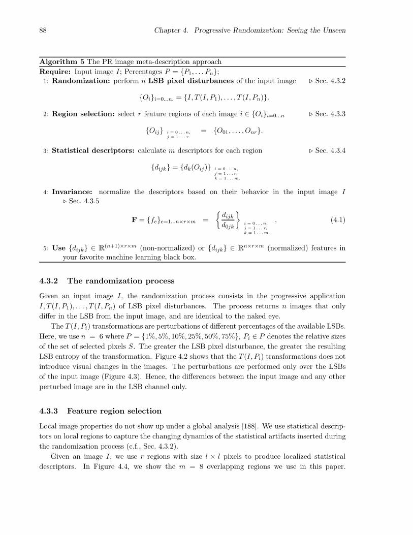
88 Chapter 4. Progressive Randomization: Seeing the Unseen
Algorithm 5 The PR image meta-description approach
Require: Input image I; Percentages P = P1, . . . Pn;1: Randomization: perform n LSB pixel disturbances of the input image ⊲ Sec. 4.3.2
Oii=0...n. = I, T (I, P1), . . . , T (I, Pn).
2: Region selection: select r feature regions of each image i ∈ Oii=0...n ⊲ Sec. 4.3.3
Oij i = 0 . . . n,
j = 1 . . . r.
= O01, . . . , Onr.
3: Statistical descriptors: calculate m descriptors for each region ⊲ Sec. 4.3.4
dijk = dk(Oij) i = 0 . . . n,
j = 1 . . . r,
k = 1 . . . m.
4: Invariance: normalize the descriptors based on their behavior in the input image I⊲ Sec. 4.3.5
F = fee=1...n×r×m =
dijk
d0jk
i = 0 . . . n,
j = 1 . . . r,
k = 1 . . . m.
, (4.1)
5: Use dijk ∈ R(n+1)×r×m (non-normalized) or dijk ∈ R
n×r×m (normalized) features inyour favorite machine learning black box.
4.3.2 The randomization process
Given an input image I, the randomization process consists in the progressive application
I, T (I, P1), . . . , T (I, Pn) of LSB pixel disturbances. The process returns n images that only
differ in the LSB from the input image, and are identical to the naked eye.
The T (I, Pi) transformations are perturbations of different percentages of the available LSBs.
Here, we use n = 6 where P = 1%, 5%, 10%, 25%, 50%, 75%, Pi ∈ P denotes the relative sizes
of the set of selected pixels S. The greater the LSB pixel disturbance, the greater the resulting
LSB entropy of the transformation. Figure 4.2 shows that the T (I, Pi) transformations does not
introduce visual changes in the images. The perturbations are performed only over the LSBs
of the input image (Figure 4.3). Hence, the differences between the input image and any other
perturbed image are in the LSB channel only.
4.3.3 Feature region selection
Local image properties do not show up under a global analysis [188]. We use statistical descrip-
tors on local regions to capture the changing dynamics of the statistical artifacts inserted during
the randomization process (c.f., Sec. 4.3.2).
Given an image I, we use r regions with size l × l pixels to produce localized statistical
descriptors. In Figure 4.4, we show the m = 8 overlapping regions we use in this paper.
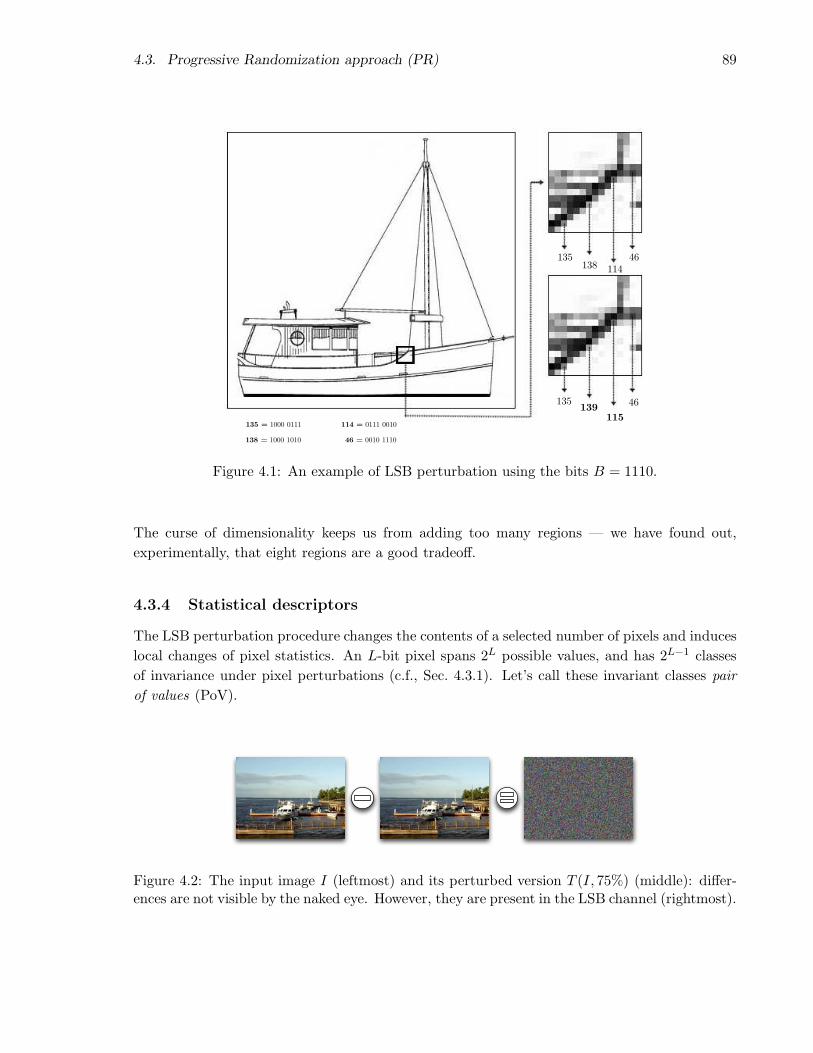
4.3. Progressive Randomization approach (PR) 89
135 = 1000 0111
138 = 1000 1010
114 = 0111 0010
46 = 0010 1110
135138 114
46
135139
115
46
Figure 4.1: An example of LSB perturbation using the bits B = 1110.
The curse of dimensionality keeps us from adding too many regions — we have found out,
experimentally, that eight regions are a good tradeoff.
4.3.4 Statistical descriptors
The LSB perturbation procedure changes the contents of a selected number of pixels and induces
local changes of pixel statistics. An L-bit pixel spans 2L possible values, and has 2L−1 classes
of invariance under pixel perturbations (c.f., Sec. 4.3.1). Let’s call these invariant classes pair
of values (PoV).
Figure 4.2: The input image I (leftmost) and its perturbed version T (I, 75%) (middle): differ-ences are not visible by the naked eye. However, they are present in the LSB channel (rightmost).

90 Chapter 4. Progressive Randomization: Seeing the Unseen
Input I
LSBs(I) T (I, 1%)
T (I, 5
%)
T(I
, 10%
)
T(I
,25%
) T(I, 75%
)
T (I, 50%)
Figure 4.3: The Progressive Randomization behavior over the LSBs. T (I, Pi) represents a PRperturbation with percentage Pi over the LSBs of the input image I.
When we disturb all the available LSBs in S with a sequence B, the distribution of 0/1 values
of a PoV will be the same as in B. The statistical analysis compares the theoretically expected
frequency distribution of the PoVs with the observed ones after the perturbation process.
We apply the χ2 (chi-squared test) [191] and UT (Ueli Maurer Universal Test) [102] to analyze
the images.
χ2 test
The χ2 test [48] compares two histograms f obs and f exp. Histogram f obs represents the obser-
vations and f exp represents the expected histogram. The procedure computes the sum of the
square differences of f obs and f exp divided by f exp,
χ2 =∑
i
(f obsi − f exp
i )2
f expi
. (4.3)
Ueli test
The Ueli test (UT ) [102] is an effective way to evaluate the randomness of a given sequence of
numbers. UT splits an input data S into n blocks. For each block bi, it analyzes each of the n−1

4.3. Progressive Randomization approach (PR) 91
Figure 4.4: The eight overlapping regions used in the experiments.
remaining blocks, looks for the most recent occurrence of bi, and takes the log of the summed
temporal occurrences. Let B(S) = (b1, b2, . . . , bN ) be a set of n blocks such that ∪∀bi= S.
Let |bi| = L be the block size for each i and |B(S)| = N be the number of blocks. We define
UT : B(S)→ R+ as a function
UT (B(S)) =1
K
Q+K∑
i=Q
ln A(bi), (4.4)
where K is the number of analyzed bits (e.g., K = N), Q is a shift in B(S) (e.g., Q = K10 [102]),
and
A(bi) =
i 6 ∃i′ ∈ N, i′ < i→ bi′ = bi,
mini′ : bi′ = bi otherwise.
In practice, if UT is close to 7.1836, we have a high randomness condition. On the other
hand, the lower UT , the more predictable is the condition in S.
4.3.5 Invariance
In some situations, it is necessary to use an image-invariant feature vector. For that, we use
the variation rate of our statistical descriptors with regard to the PR, rather than their values.
We normalize all descriptors from the transformations with regard to their values in the input
image
F = fee=1...n×r×m =
dijk
d0jk
i = 0 . . . n,
j = 1 . . . r,
k = 1 . . . m.
, (4.5)
where d denotes a descriptor 1 ≤ k ≤ m of a region 1 ≤ j ≤ r of an image 0 ≤ i ≤ n and F is
the final generated descriptor vector of the image I. Figures 4.5(a-b) show the behavior of our
statistical descriptors along the progressive randomization of one selected image I.

92 Chapter 4. Progressive Randomization: Seeing the Unseen
BaseT1
T2
T3
T4
T5
T6
T1 T2 T3 T4 T5 T6
PR transformation
χ2
des
crip
tor
valu
e
0
0.2
0.4
0.6
0.8
1
1.2
(a) χ2 descriptor.
BaseT1
T2
T3
T4
T5
T6
T1 T2 T3 T4 T5 T6
PR transformation
UT
des
crip
tor
valu
e
0.81
0.82
0.83
0.84
0.85
0.86
0.87
0.88
0.89
0.9
0.91
(b) UT descriptor.
Figure 4.5: Normalized descriptor’s behavior along the progressive randomization. Ti representsthe PR operation T (I, Pi).
The need for invariance depends on the application. For instance, it is necessary for Ste-
ganalysis but harmful for Image Categorization. In Steganalysis, we want to differentiate images
that do not contain hidden messages from those that contain hidden messages, and the image
class is not important. On the other hand, in Image Categorization, the descriptor values are
important to improve the class differentiation. Different classes do have distinct behavior under
Progressive Randomization approach (c.f., Sec. 4.4, 4.5, and 4.6).
4.4 Experiments and results – Image Categorization
In this section, we describe how we train, test and validate PR image meta-description approach
for Image Categorization. We validate the multi-class classification as a complete self-contained
classification procedure in Experiment 1. In that experiment, we use a 40,000-image database
with 12,000 outdoors, 10,000 indoors, 13,500 art photographs, and 4,500 computer generated
images (CGIs) with three different classification approaches.
The images in Experiment 1 come from five main sources: Mark Harden’s Artchive1, the
European Web Gallery of Art2, FreeFoto34, Berkeley CalPhotos5, and from The Internet Ray
Tracing Competition (IRTC)6. Figure 4.6 show some examples of each category.
We also validate the PR image meta-description approach in three other categorization
1http://www.artchive.com2http://www.wga.hu3http://www.freefoto.com4http://www.ic.unicamp.br/~rocha/pub/communications.html5http://calphotos.berkeley.edu6http://www.irtc.org

4.4. Experiments and results – Image Categorization 93
(a) Outdoors. c©FreeFoto. (b) Indoors. Personalcollection.
(c) Arts. Portrait of Nicolaes Ruts by Rembrandtvan Rijn and A Farmstead Near a Stream by Cor-nelis Saftleven.
(d) Computer Generated Images. Autoban byJaime Vives Piqueres and Glasses by GillesTran.
Figure 4.6: Examples of each analyzed category: Outdoors, Indoors, CGIs, and Arts.
scenarios. In Experiment 2, we provide another interpretation of Experiment 1 using a
second carefully assembled image database. In Experiment 3, we perform a 9-class image
categorization using 3,354 FreeFoto photographs. Finally, Experiment 4, we perform a 15-
class image categorization using 2,950 images of fruits.
4.4.1 Experiment 1
We compare our method to the state of the art two-class separation approaches in the lit-
erature [34, 92, 94, 128, 162] using a simple Bagging ensemble of Linear Discriminant Analysis
(BLDA) [55]. Furthermore, we also perform multi-class image-categorization, separating Out-
door photographs, Art images, Photorealistic Computer Generated Images, and Indoors pho-
tographs. Here, we use the BLDA classifier with 13 iterations and 10-fold cross validation.
Two-class classification
Cutzu et al. [34] have addressed the problem of differentiating photographs of real scenes from
photographs of art works. They validated over a database with 6,000 photographs from FreeFoto
and 6,000 photographs from Mark Harden’s Artchive and from Indiana Image Collection7.
The authors have used color and intensity edges, color variation, saturation, and Gabor
features in a complex classifier. We use a similar image set reported in [34]. We have selected
7http://www.dlib.indiana.edu/collections/dido
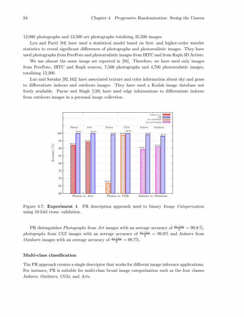
94 Chapter 4. Progressive Randomization: Seeing the Unseen
12,000 photographs and 13,500 art photographs totalizing 25,500 images.
Lyu and Farid [94] have used a statistical model based on first- and higher-order wavelet
statistics to reveal significant differences of photographs and photorealistic images. They have
used photographs from FreeFoto and photorealistic images from IRTC and from Raph 3D Artists.
We use almost the same image set reported in [94]. Therefore, we have used only images
from FreeFoto, IRTC and Raph sources, 7,500 photographs and 4,700 photorealistic images,
totalizing 12,200.
Luo and Savakis [92,162] have associated texture and color information about sky and grass
to differentiate indoors and outdoors images. They have used a Kodak image database not
freely available. Payne and Singh [128] have used edge informations to differentiate indoors
from outdoors images in a personal image collection.
92.0%
99.9%
94.0%
99.9%
66.8%
99.8% 98.8%99.9%
89.3%
99.8%
91.0%
99.7%
Photos Arts Photos CGIs Indoors Outdoors
Cutzu et al.PR
Lyu and Farid
Luo and Savakis
Acc
ura
cy(%
)
Photos vs. Arts Photos vs. CGIs Indoors vs. Outdoors60
65
70
75
80
85
90
95
100
Figure 4.7: Experiment 1. PR description approach used to binary Image Categorizationusing 10-fold cross- validation.
PR distinguishes Photographs from Art images with an average accuracy of µ1+µ2
2 = 99.9.%,
photographs from CGI images with an average accuracy of µ1+µ2
2 = 99.9% and Indoors from
Outdoors images with an average accuracy of µ1+µ2
2 = 99.7%.
Multi-class classification
The PR approach creates a single descriptor that works for different image inference applications.
For instance, PR is suitable for multi-class broad image categorization such as the four classes
Indoors, Outdoors, CGIs, and Arts.

4.4. Experiments and results – Image Categorization 95
In order to validate the multi-class classification, we have used two different approaches that
are combinations of binary classifiers: All Pairs majority voting of the binary classifier BLDA
(All-Pairs-BLDA); and Support Vector Machines (SVMs). LibSVM uses an internal mechanism
that put together all 1 × 1 combinations of the classes and performs a majority voting in the
final stage. We have used the radial basis function SVM. All-Pairs-BLDA uses sets of binary
classifiers. Note that, any other binary classifier could be used rather than All-Pairs-BLDA.
Tables 4.1 and 4.2 show the resulting classification using All-Pairs-BLDA, and SVMs. The
diagonal represents the classification accuracy. For instance, using All-Pairs-BLDA multi-class
approach 89.4%, of the images that represent an Art scenario are correctly classified, while only
8.17% of them are misclassified as Indoors.
All-Pairs-BLDA PredictionsArts CGIs Indoors Outdoors
Arts 89.4% ± 1.04% 4.41% ± 0.49% 6.16% ± 0.80% 0.00% ± 0.00%CGIs 33.66% ± 2.36% 53.3% ± 2.09% 13.0% ± 1.22% 0.00% ± 0.00%
Indoors 8.97% ± 0.54% 5.58% ± 0.34% 85.44% ± 0.62% 0.01% ± 0.03%Outdoors 0.00% ± 0.00% 0.06% ± 0.07% 0.02% ± 0.05% 99.9% ± 0.11%
Table 4.1: Experiment 1. PR multi-class Image Categorization using All-Pairs-BLDA.
The PR approach is independent of the multi-class technique. Figure 4.8 shows the minimum
accuracy of the two approaches as well as the average accuracy and the geometric average
accuracy.
All-Pairs-BLDAlibSVM
Average Acc Geometric Average AccMinimum Acc
Acc
ura
cy(%
)
56.9%
52.9%
82.6%
82.0%
80.9%
79.8%
min(Di)
1|D|
∑
Di|D|√∏
Di
40
45
50
55
60
65
70
75
80
85
90
95
100
Figure 4.8: Experiment 1. Multi-class overall accuracy. D is the diagonal of the confusionmatrix.

96 Chapter 4. Progressive Randomization: Seeing the Unseen
SVM PredictionsArts CGIs Indoors Outdoors
Arts 86.4% ± 1.16% 2.10% ± 0.43% 11.5% ± 0.85% 0.00% ± 0.00%CGIs 36.2% ± 2.32% 45.3% ± 1.55% 18.2% ± 1.34% 0.20% ± 0.20%
Indoors 17.5% ± 1.28% 4.90% ± 0.41% 77.6% ± 1.47% 0.00% ± 0.00%Outdoors 0.02% ± 0.03% 0.37% ± 0.18% 0.01% ± 0.03% 99.6% ± 0.21%
Table 4.2: Experiment 1. PR multi-class Image Categorization using SVM.
4.4.2 Experiment 2
Experiment 1 provides good performance in two-class and multi-class categorization. However,
some can argue that the number of training examples is too large and that it might have suffered
from bias due to different compression applied to each category, given that they come from
different sources. It is important to notice that almost all images come from well known image
repositories and most of them are built up from user contributions.
So, we have created a second scenario for multi-class categorization of Indoors, Outdoors,
CGIs and Art photographs. In this experiment, we have manually selected 500 images for each
class totalizing 2,000 images. Each category contains images from at least 75 different internet
sources and there are no more than seven images from the same place. There is no intersection
among the images in this scenario with the scenario presented in Experiment 1. In this
experiment, there are at least 400 different cameras with many different compression scenarios.
Figure 4.9 presents the results using the All-Pairs BLDA multi-class approach with 13 iterations.
We show that the results using PR descriptor are not biased due to possible different com-
pression levels. The results are better than the priors of each class (about 25% per class).
Therefore, the PR descriptor provides good separation among classes. Even with few training
examples, the descriptor still presents a good performance. The more examples we provide in
the training phase, the better the classification performance (Figure 4.9).
4.4.3 Experiment 3
Here, we select 3,354 images from FreeFoto and divide them into nine classes. Figure 4.10 shows
some examples of each category. Sky and Clouds category represents sunny and clear days. Cum-
mulonimbus Clouds comprises images associated with heavy precipitation and thunderstorms.
The other categories are self explanatory.
We do not pre-process any image. All images come from FreeFoto and were originally stored
in JPEG format with 72 DPIs using similar compression levels. Figure 4.11 presents the results
for this experiment using the All-Pairs BLDA multi-class approach with 13 iterations.
The PR meta-description approach generalyzes from the priors (about 19 for each category).
The accuracy increases with the number of training examples (left plot of Figure 4.11). The
more images in the training phase, the more accurate the classification. This suggests that
PR technique can be combined with other image descriptors for categorization purposes. The
average standard deviation σ is bellow 5%. For all classes, the classification results are far above

4.5. Experiments and results – Steganalysis 97
Acc
ura
cy(%
)
Training Size Per Class
Minimum AccuracyAverage Accuracy
Geometric Average Accuracy
028
30
32
34
36
38
40
42
50 100 150 200 250 300 350 400 450
Acc
ura
cy(%
)
Classes
Average accuracy
38.8%
35.7%
41.6%
45.7%
Ou
tdoor
s
Ind
oor
s
CG
Is
Art
s
0
10
20
30
40
50
60
Figure 4.9: Experiment 2. Out × Ind × CGI × Arts using All-Pairs BLDA(13) .:. 4 classes.Left plot : average performance for variable training sizes. Right plot : class’ performance for450-sized training sets.
the expected priors (2σ minimum).
4.4.4 Experiment 4
In this experiment, we perform categorization of images of fruits8 and we want to show that the
PR results are not biased due to camera properties. Here, we have used the same camera and
setup in the capture. The JPEG compression level is the same for all images.
We personally acquired the 2,950 images at our local fruits and vegetables distribution center
(CEASA), using a Canon PowerShot P1 camera, at a resolution of 1, 024× 768 against a white
background. Figure 4.12 depicts the 15 different classes. Even in the same category, there are
many illumination differences (Figure 4.13).
Figure 4.14 presents the results for this experiment using the All-Pairs BLDA multi-class
approach with 13 iterations. Clearly, PR generalyzes from the priors (about 115 for each category)
and the accuracy increases with the number of training examples (left plot of Figure 4.14).
4.5 Experiments and results – Steganalysis
In this section, we describe how we train, test and validate the PR image meta-description
approach for Steganalysis. In this scenario, our objective is to detect whether or not a given image
contains an embedded content. Here, we have used the same image database of Experiment 1
in Section 4.4.1.
8http://www.ic.unicamp.br/~rocha/pub/communications.html
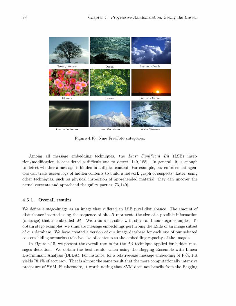
98 Chapter 4. Progressive Randomization: Seeing the Unseen
Trees / Forests Ocean Sky and Clouds
Flowers Leaves Sunrise / Sunset
Cummulonimbus Snow Mountains Water Streams
Figure 4.10: Nine FreeFoto categories.
Among all message embedding techniques, the Least Significant Bit (LSB) inser-
tion/modification is considered a difficult one to detect [149, 188]. In general, it is enough
to detect whether a message is hidden in a digital content. For example, law enforcement agen-
cies can track access logs of hidden contents to build a network graph of suspects. Later, using
other techniques, such as physical inspection of apprehended material, they can uncover the
actual contents and apprehend the guilty parties [73,149].
4.5.1 Overall results
We define a stego-image as an image that suffered an LSB pixel disturbance. The amount of
disturbance inserted using the sequence of bits B represents the size of a possible information
(message) that is embedded |M |. We train a classifier with stego and non-stego examples. To
obtain stego examples, we simulate message embeddings perturbing the LSBs of an image subset
of our database. We have created a version of our image database for each one of our selected
content-hiding scenarios (relative size of contents to the embedding capacity of the image).
In Figure 4.15, we present the overall results for the PR technique applied for hidden mes-
sages detection. We obtain the best results when using the Bagging Ensemble with Linear
Discriminant Analysis (BLDA). For instance, for a relative-size message embedding of 10%, PR
yields 78.1% of accuracy. That is almost the same result that the more computationally intensive
procedure of SVM. Furthermore, it worth noting that SVM does not benefit from the Bagging

4.5. Experiments and results – Steganalysis 99
Acc
ura
cy(%
)
Training Size Per Class
Minimum AccuracyAverage Accuracy
Geometric Average Accuracy
10 50 60 7015
20
20
25
30
30
35
40
40
45
Acc
ura
cy(%
)
Classes
Average accuracy
Tre
es/F
ores
ts
Oce
an
Sky/C
lou
ds
Flo
wer
s
Lea
ves
Su
nri
se/S
un
set
Cu
mu
lon
imb
us
Clo
ud
s
Ice
Mon
tain
s
Wat
erS
trea
ms
0
10
50
60
70
20
30
40
30.9%
44.1%
29.5%
36.5% 36.0%37.9%
58.2%
41.3%43.5%
Figure 4.11: Experiment 3. FreeFoto categorization using All-Pairs BLDA(13) .:. 9 classes.Left plot : average performance for variable training sizes. Right plot : class’ performance for70-sized training sets.
ensemble. That is because SVM uses only the elements close to the margins in the classification
procedure.
PR descriptor scales with the number of examples in the training stage. Overall, the more
examples we provide in the training phase, the greater the detection accuracy regardless the
message size. In Figure 4.16, we present the PR descriptor with different training set sizes.
The detection of very small relative-size contents is very hard, and still an open problem.
Nevertheless, in practical situations, like when pornographers use images to sell their child-porn
images, they usually use a reasonable portion of the LSB channel available space (e.g., 25%). In
this class of problem, PR meta-description approach detects such activities with accuracy just
under 90% which shows that it is an effective approach for embedding content detection.
4.5.2 Class-based Steganalysis
Different classes/categories of images have a very distinct behavior in properties. We explored
their different LSB behavior earlier in this paper for proper image categorization.
In this section, we show how the PR descriptor is still able to perform Steganalysis despite
all these differences, and gives us a strong insight about which types of images are better for
information hiding.
We have found that the detection of hidden content in images with low richness of detail
(e.g., Indoors) is easier. The inserted artifacts of the embedding process in these images are more
obvious than those artifacts inserted in images with more complex details. In these experiment,
we have considered four image classes Outdoors, Indoors, Arts, and CGIs. We have used the
same image database of Experiment 1 in Section 4.4.1.
In each analysis, we train our classifier with examples sampled without replacement from
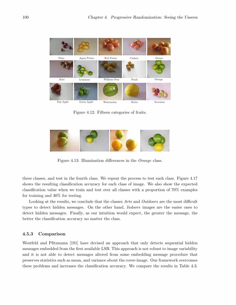
100 Chapter 4. Progressive Randomization: Seeing the Unseen
Plum Agata Potato Red Potato Cashew Onions
Kiwi OrangeLemmons
Fuji Apple Green Apple Watermelon Melon Nectarine
Williams Pear Peach
Figure 4.12: Fifteen categories of fruits.
Figure 4.13: Illumination differences in the Orange class.
three classes, and test in the fourth class. We repeat the process to test each class. Figure 4.17
shows the resulting classification accuracy for each class of image. We also show the expected
classification value when we train and test over all classes with a proportion of 70% examples
for training and 30% for testing.
Looking at the results, we conclude that the classes Arts and Outdoors are the most difficult
types to detect hidden messages. On the other hand, Indoors images are the easier ones to
detect hidden messages. Finally, as our intuition would expect, the greater the message, the
better the classification accuracy no matter the class.
4.5.3 Comparison
Westfeld and Pfitzmann [191] have devised an approach that only detects sequential hidden
messages embedded from the first available LSB. This approach is not robust to image variability
and it is not able to detect messages altered from some embedding message procedure that
preserves statistics such as mean, and variance about the cover-image. Our framework overcomes
these problems and increases the classification accuracy. We compare the results in Table 4.3.

4.5. Experiments and results – Steganalysis 101
Acc
ura
cy(%
)
Training Size Per Class
Minimum AccuracyAverage Accuracy
Geometric Average Accuracy
015
20
20
25
30
35
40
40
45
50
55
60
60
65
70
80 100 120 140
Acc
ura
cy(%
)
Classes
Average accuracy
Plu
m
Aga
taP
otat
o
Ast
erix
Red
Pot
ato
Cas
hew
On
ion
Kiw
i
Ora
nge
Lem
on
Fu
jiA
pp
le
Gra
nn
-Sm
ith
Ap
ple
Wat
erm
elon
Hon
eyd
ewM
elon
Nec
tari
ne
William
sP
ear
Pea
ch
79.4%
56.8%
68.4%
79.5%
59.1%
42.9%
50.0%
71.6%
77.8%
58.5%
71.5%
61.2%63.5%
70.7%73.0%
0
20
40
60
80
100
Figure 4.14: Experiment 4. Fruits categorization using All-Pairs BLDA(13) .:. 15 classes.Left plot : average performance for variable training sizes. Right plot : class’ performance for140-sized training sets.
In this experiment, we have used the SVM binary classifier [16].
Other approaches for Steganalysis include the works of Shi et al. [168],
Pevny and Fridrich [134], and Goljan et al. [59]. However, these approaches have been
designed for embedding techniques based on lossy compression properties such as those present
in JPEG images. In this paper, we present a detection framework designed for lossless
embedding detection.
It is not intended that PR outperforms all the best Steganalysis algorithms in the literature.
It is worth noting that we are not providing a complete Steganalysis framework. Indeed, in this
paper, we present a new image meta-description approach that can be used for Steganalysis.
For this reason, we compare our descriptor with two well-known state-of-the-art solutions. PR
association with other image descriptors is straightforward.
WP PR
µ± σ µ± σ
01% 52.6% ± 0.1% 54.1% ± 0.9%
05% 52.6% ± 0.1% 70.7% ± 0.9%
10% 54.6% ± 4.1% 80.2% ± 0.5%
25% 72.9% ± 1.9% 89.3% ± 0.6%
50% 83.0% ± 0.6% 94.0% ± 0.5%
75% 84.8% ± 0.9% 96.3% ± 0.3%
Table 4.3: Westfeld and Pfitzmann’s detection approach (WP) vs. Progressive Randomiza-tion (PR). µ and σ from cross-validation.
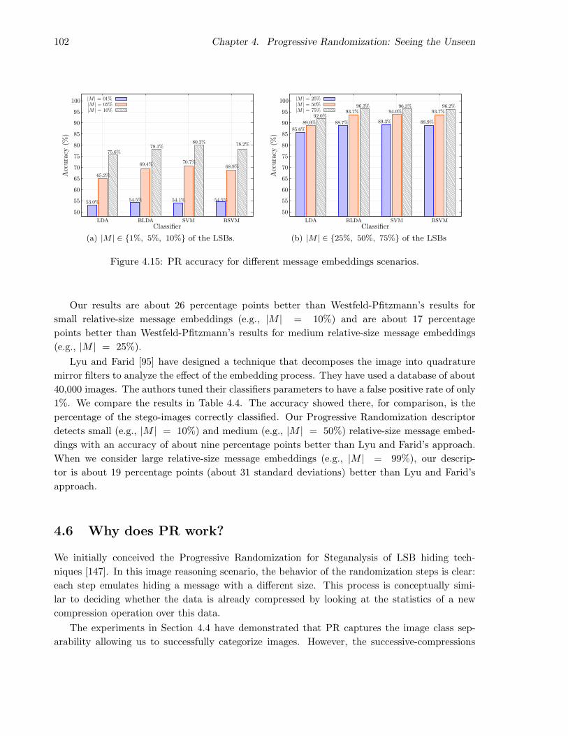
102 Chapter 4. Progressive Randomization: Seeing the Unseen
LDA BLDA SVM BSVM
|M | = 01%|M | = 05%|M | = 10%
Acc
ura
cy(%
)
Classifier
50
55
60
65
70
75
80
85
90
95
100
53.0%
65.2%
75.6%
54.5%
69.4%
78.1%
54.1%
70.7%
80.2%
54.5%
68.9%
78.2%
(a) |M | ∈ 1%, 5%, 10% of the LSBs.
LDA BLDA SVM BSVM
|M | = 25%|M | = 50%|M | = 75%
Acc
ura
cy(%
)
Classifier
50
55
60
65
70
75
80
85
90
95
100
85.6%
89.0%
92.0%
88.7%
93.7%96.3%
89.3%
94.0%96.3%
88.9%
93.7%96.2%
(b) |M | ∈ 25%, 50%, 75% of the LSBs
Figure 4.15: PR accuracy for different message embeddings scenarios.
Our results are about 26 percentage points better than Westfeld-Pfitzmann’s results for
small relative-size message embeddings (e.g., |M | = 10%) and are about 17 percentage
points better than Westfeld-Pfitzmann’s results for medium relative-size message embeddings
(e.g., |M | = 25%).
Lyu and Farid [95] have designed a technique that decomposes the image into quadrature
mirror filters to analyze the effect of the embedding process. They have used a database of about
40,000 images. The authors tuned their classifiers parameters to have a false positive rate of only
1%. We compare the results in Table 4.4. The accuracy showed there, for comparison, is the
percentage of the stego-images correctly classified. Our Progressive Randomization descriptor
detects small (e.g., |M | = 10%) and medium (e.g., |M | = 50%) relative-size message embed-
dings with an accuracy of about nine percentage points better than Lyu and Farid’s approach.
When we consider large relative-size message embeddings (e.g., |M | = 99%), our descrip-
tor is about 19 percentage points (about 31 standard deviations) better than Lyu and Farid’s
approach.
4.6 Why does PR work?
We initially conceived the Progressive Randomization for Steganalysis of LSB hiding tech-
niques [147]. In this image reasoning scenario, the behavior of the randomization steps is clear:
each step emulates hiding a message with a different size. This process is conceptually simi-
lar to deciding whether the data is already compressed by looking at the statistics of a new
compression operation over this data.
The experiments in Section 4.4 have demonstrated that PR captures the image class sep-
arability allowing us to successfully categorize images. However, the successive-compressions

4.6. Why does PR work? 103
Acc
ura
cy(%
)T = 01%
50
52
54
56
58
60
2,500 5,000 7,500 10,000 12,500 15,000 17,500 20,000
(a) |M | = 1%.
Acc
ura
cy(%
)
T = 05%
T = 10%
66
68
70
72
74
76
78
80
2,500 5,000 7,500 10,000 12,500 15,000 17,500 20,000
(b) |M | ∈ 5%, 10%.
Acc
ura
cy(%
)
T = 25%
T = 50%
86
88
90
92
94
2,500 5,000 7,500 10,000 12,500 15,000 17,500 20,000
(c) |M | ∈ 25%, 50%.
Acc
ura
cy(%
)
T = 75%
96
98
100
2,500 5,000 7,500 10,000 12,500 15,000 17,500 20,000
(d) |M | = 75%.
Figure 4.16: PR accuracy for different training set sizes and stego scenarios.
analogy, so intuitive in Steganalysis, is not convincing for this new problem. Our conjecture
is that the distinct class behavior comes from the interaction between different light spectrum
and the sensors during the acquisition process. That supports that fact that Outdoors is easier
to differentiate from the other classes, and that Indoors and Arts are harder to differentiate
amongst each other, as both use artificial illumination.
To show that the separability is not due to different patterns of luminance/color amongst
classes, we have devised an experiment to measure the expected value of the Ueli descriptor
conditioned to the luminance of the region.
We use a local sliding window to calculate local luminance and Ueli, and compute them on all
possible 32× 32-pixel windows in 300 examples of each class to estimate the E[UT |Lum,Class],
the conditional expectation of Ueli for given luminance and class.
We approximate the continuous function using histograms of expected values of UT for each

104 Chapter 4. Progressive Randomization: Seeing the Unseen
Acc
ura
cy(%
)
Relative message size|M | = 1% |M | = 5% |M | = 10%
51.7%50.3%
47.7%
51.0%52.8%
55.2%55.8%
61.9%
69.5%
64.3%
60.1%
64.7%
68.5%
81.7%
73.2%
Arts
Indoors
Outdoors
CGIs
Expected value
45
50
55
60
65
70
75
80
85
90
95
100
(a)
Acc
ura
cy(%
)
Relative message size|M | = 25% |M | = 50% |M | = 75%
76.4%
81.0%
78.3%
93.3%
85.9%88.6%
90.2%89.4%
95.5%93.5% 94.6%
95.2%95.1%
98.5%96.4%
Arts
Indoors
Outdoors
CGIs
Expected value
45
50
55
60
65
70
75
80
85
90
95
100
(b)
Figure 4.17: PR Steganalysis along with different image classes and different relative messagesizes.
class HEi , i ∈ Outdoor, Indoor
HEi ← E[Ueli|L ∈ 1 . . . 255], (4.6)
where E[.] is the statistical expectation, and L is the luminance such that L = (0.3∗R)+(0.59∗G) + (0.11 ∗B).
The upper plot of Figure 4.18 displays the Ueli conditional expectation for unmodified Out-
doors and Indoors classes. There is a consistent difference between classes, showing that the
separability of the LSB statistical descriptors is not due to different class patterns of luminance.
We also observe the effect of the limited dynamic range on the statistical descriptor. Lumi-
nance components that are too small are squished to zero, while color components that should
be very high are clamped to the maximum (255 in the 8-bit case). In these extreme cases, there
is no randomness, and the Ueli value goes down to zero. As we calculate the expected values in
sliding windows, the decrease along the borders of the dynamic range demonstrate the decrease
of the randomness as more elements of the window are clamped to an extreme value.
4.7 Limitations
In this paper, we have introduced a new image meta-description approach. Its main difference
with respect to the state-of-the-art techniques is that it is based on controlled perturbations on
least significant properties of images.
PR technique is not intended to be the final word for Image Categorization and Steganalysis
on its own. Of course, there are some limitations with the method. First of all, it is more suitable
for loss-less images or high-quality lossy-compressed images, i.e., if one performs a medium-to-

4.8. Conclusions and remarks 105
LDA SVM-RBF Type
µ σ µ σ
01%1.3% – 1.9% – LF3.2% 0.5% 3.6% 1.0% PR
10%2.8% – 6.2% – LF7.0% 0.8% 15.8% 1.1% PR
50%16.8% – 44.7% – LF24.2% 1.5% 53.1% 1.6% PR
99%42.3% – 78.0% – LF95.8% 0.5% 97.0% 0.6% PR
Table 4.4: Lyu and Farid’s detection approach (LF) vs. Progressive Randomization (PR) con-sidering FPR = 1%. µ and σ from cross-validation. Lyu and Farid’s results from [95].
high-rate lossy compression (e.g., +25% of loss), it is possible that the method will fail. However,
there are a lot of available images in the internet with low-to-medium compression levels.
In the case of Steganalysis, if one destroys the LSB channel information using a pseudo-
random number generator (PRNG), the method potentially will fail. However, in this case, even
the message will be destroyed.
Finally, PR technique probably will fail when used for Image Categorization of images ac-
quired with old cameras with low-quality capturing sensors. In such situations, it is likely
that the LSB channel information is related to noise in the process of acquisition. Hence, the
relationship of the LSB channel with the other bit channels becomes weaker.
4.8 Conclusions and remarks
We have introduced a new image descriptor descriptor that captures the changing dynamics of
the statistical artifacts inserted during a perturbation process in each of the broad-image classes
of our interest.
We have applied and validated the Progressive Randomization descriptor in two real image
inference scenarios: Image Categorization and Steganalysis.
The main difference among PR and the state-of-the-art algorithms is that it is based on
perturbations on the values of the Least Significant Bits of images. With such perturbations,
PR captures the image class separability allowing us to successfully infer high-level information
about images. Our conjecture is that the interaction of different light spectrum with the camera
sensors induces different patterns in the LSB field. PR does not consider semantical information
about scenes.
The most important features in the PR descriptor are its low dimensionality and its unified
approach for different applications (e.g., the class of an image, the class of an object in a restricted
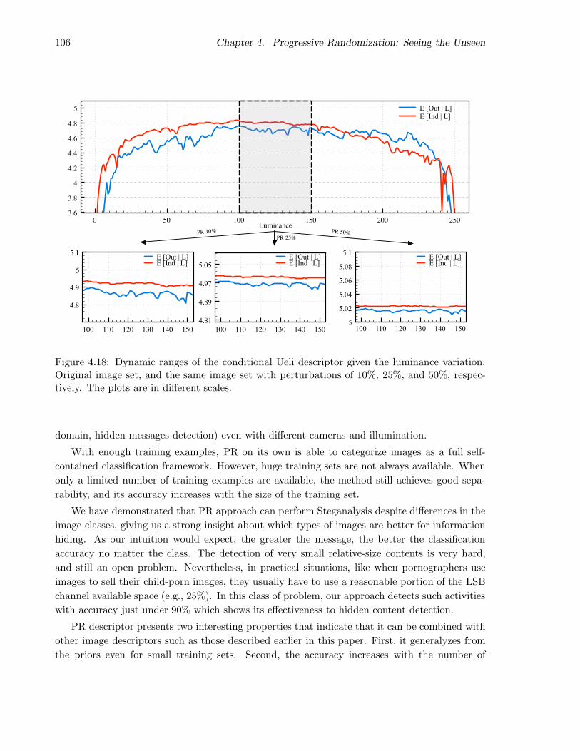
106 Chapter 4. Progressive Randomization: Seeing the Unseen
0 50 100 150 200 250
3.6
3.8
4
4.2
4.4
4.6
4.8
5 E [Out | L]E [Ind | L]
LuminancePR 10%
PR 25%
PR 50%
100 110 120 130 140 150
4.8
4.9
5
5.1E [Out | L]E [Ind | L]
100 110 120 130 140 150
4.81
4.89
4.97
5.05
E [Out | L]E [Ind | L]
100 110 120 130 140 1505
5.02
5.04
5.06
5.08
5.1E [Out | L]E [Ind | L]
Figure 4.18: Dynamic ranges of the conditional Ueli descriptor given the luminance variation.Original image set, and the same image set with perturbations of 10%, 25%, and 50%, respec-tively. The plots are in different scales.
domain, hidden messages detection) even with different cameras and illumination.
With enough training examples, PR on its own is able to categorize images as a full self-
contained classification framework. However, huge training sets are not always available. When
only a limited number of training examples are available, the method still achieves good sepa-
rability, and its accuracy increases with the size of the training set.
We have demonstrated that PR approach can perform Steganalysis despite differences in the
image classes, giving us a strong insight about which types of images are better for information
hiding. As our intuition would expect, the greater the message, the better the classification
accuracy no matter the class. The detection of very small relative-size contents is very hard,
and still an open problem. Nevertheless, in practical situations, like when pornographers use
images to sell their child-porn images, they usually have to use a reasonable portion of the LSB
channel available space (e.g., 25%). In this class of problem, our approach detects such activities
with accuracy just under 90% which shows its effectiveness to hidden content detection.
PR descriptor presents two interesting properties that indicate that it can be combined with
other image descriptors such as those described earlier in this paper. First, it generalyzes from
the priors even for small training sets. Second, the accuracy increases with the number of

4.8. Conclusions and remarks 107
training examples in all applications we have showed.
Future work include: to select image regions rich in details and analyze how they are affected
using PR descriptor; to investigate other statistical descriptors besides χ2 and UT such as kurtosis
and skewness; and to apply PR descriptor to other image inference scenarios such as image
forgery detection.


Fusao Multi-classe de Caracterısticas
e Classificadores
Algumas vezes, problemas de categorizacao multi-classe sao complexos e a fusao de informacoes
de varios descritores torna-se importante.
Embora a fusao de caracterısticas seja bastante eficaz para alguns problemas, ela pode produ-
zir resultados inesperados quando as diferentes caracterısticas nao estao normalizadas e prepara-
das de forma adequada. Alem disso, esse tipo de combinacao tem a desvantagem de aumentar o
numero de caracterısticas do vetor base de descricao o que, por sua vez, pode levar a necessidade
de mais elementos para o treinamento.
No Capıtulo 5, nos apresentamos uma abordagem para combinar classificadores e carac-
terısticas capaz de lidar com a maior parte dos problemas citados anteriormente. Nosso objetivo
e combinar um conjunto de caracterısticas e os classificadores mais apropriados para cada uma
de modo a melhorar a performance sem comprometer a eficiencia.
Nos propomos lidar com um problema multi-classe a partir da combinacao de um conjunto de
classificadores binarios. Nos validamos nossa abordagem numa aplicacao real para classificacao
automatica de frutas e legumes.
O trabalho apresentado no Capıtulo 5 e uma compilacao de nosso artigo submetido a Elsevier
Computers and Electronics in Agriculture (Compag). Os autores desse artigo, em ordem, sao:
Anderson Rocha, Daniel C. Hauagge, Jacques Wainer e Siome Goldenstein.
Este trabalho nos rendeu, inicialmente, o artigo [153] no Brazilian Symposium of Computer
Graphics and Image Processing (Sibgrapi).
109


Chapter 5
Automatic Fruit and Vegetable
Classification from Images
Abstract
In this paper, we address a multi-class fruit-and-vegetable categorization task in a semi-
controlled environment, such as a distribution center or the supermarket cashier. To solve
such a complex problem using just one feature descriptor is a difficult task and feature fusion
becomes mandatory. Although normal feature fusion is quite effective for some problems, it can
yield unexpected classification results when the different features are not properly normalized
and prepared. Besides it has the drawback of increasing the dimensionality which might require
more training data. To cope with these problems, we propose a unified approach that can com-
bine many features and classifiers, requires less training, and is more adequate to some problems
than a naıve method, where all features are simply concatenated and fed independently to each
classification algorithm. Besides that, the algorithm proposed is amenable to continuous learn-
ing, both when refining a learned model and also when adding new classes to be discriminated.
We validate the system using an image data set we collected at a local produce distribution
center. Since this data set can help further research by the overall scientific community, we also
make it publicly available over the internet.
5.1 Introduction
Recognizing different kinds of vegetables and fruits is a recurrent task in supermarkets, where
the cashier must be able to point out not only the species of a particular fruit (i.e., banana,
apple, pear) but also it’s variety (i.e., Golden Delicious, Jonagold, Fuji), which will determine it’s
price. The use of barcodes has mostly ended this problem for packaged products but given that
111

112 Chapter 5. Automatic Fruit and Vegetable Classification from Images
consumers want to pick their produce, they can not be packaged, and thus must be weighted.
A common solution to this problem is issuing codes for each kind of fruit/vegetable; which has
problems given that the memorization is hard, leading to errors in pricing.
As an aid to the cashier, many supermarkets issue a small book with pictures and codes; the
problem with this solution is that flipping over the booklet is time-consuming. In this paper, we
review several image descriptors in order to propose a system to solve the problem by adapting
a camera to the supermarket scale that identifies fruits and vegetables based on color, texture,
and appearance cues.
Formally, we state our problem in the following manner: given an image of fruits or vegetables
of only one variety, in arbitrary position and number, the system must return a list of possible
candidates of the form (species, variety). Sometimes, the object can be inside a plastic bag that
can add specular reflections and hue shifts.
Given that the big variety and the impossibility of predicting which kinds of fruit/vegetables
are sold, training must be done on site by someone with little or no technical knowledge. There-
fore, the system must be able to achieve a high level of precision with only a few training
examples (e.g., up to 30 images). Another desirable characteristic would be continuous learn-
ing. On one hand, more training data would be generated as the system commits mistakes and
the cashier corrects them. On the other hand, in this semi-supervised scenario, eventually the
operator will commit mistakes and the learning algorithm must be robust to noisy training data.
Here, we combine local and global features using different classification procedures. We used
global color histograms, local texture, shape, and correlation descriptors with distinctive fruit
parts.
Our contribution in this paper is twofold. The first is that we evaluate several image de-
scriptors in the literature and point out the best ones to solve our multi-class fruits/vegetables
categorization problem. Important questions about such descriptors are: which ones require
less training? Is it necessary to use complex approaches such as bag-of-features or constellation
models? How do the descriptors perform when increasing the number of training examples?
What combinations and parameters of the descriptors provide better effectiveness? How do the
descriptors behave under the curse-of-dimensionality? In the experiments we show answers for
such questions.
We end up with a unified approach that can combine many features and classifiers that
requires less training and is more adequate to some problems than a naıve method, where all
features are simply concatenated and fed independently to each classification algorithm. Besides
that, the algorithm proposed is amenable to continuous learning, both when refining a learned
model and also when adding new classes to be discriminated.
The second contribution is that we create an image data set collected from our local fruits and
vegetables distribution center and make it public. In general, there are a few well-documented
image data sets freely available for testing algorithm performance in image categorization and
content-based image retrieval tasks. In this context, we provide an image data set with 15
produce categories comprising 2,633 images collected on site with all its creation details. The
images were collected in a period of five months under diverse conditions.

5.2. Literature review 113
In Section 5.2, we give a brief overview of previous work in object recognition and image
categorization. In Section 5.3, we present the different kinds of image descriptors we used in
this paper as well as the produce data set. Section 5.4 presents results for diverse background
subtraction approaches and analyzes the one we used in this paper. Section 5.5, reports results
for the image data set we created for each feature and classifier with no fusion. Section 5.6 intro-
duces our solution for feature and classifier fusion, and Section 5.7 presents experimental results.
Section 5.8 draws some considerations about the proposed technique, as well as conclusions and
future directions.
5.2 Literature review
Recently, there has been a lot of activity in the area of Image Categorization. Previous ap-
proaches considered patterns in color, edge and texture properties [126, 169, 178]; low- and
middle-level features to distinguish broad classes of images [34, 98, 148, 162]; In addition, Hei-
demann [66] has presented an approach to establish image categories automatically using his-
tograms, colors and shape descriptors with an unsupervised learning method.
With respect to our problem, VeggieVision [18] was the first attempt of a supermarket
produce recognition system. The system uses color, texture and density (thus requiring extra
information from the scale). However, as this system was presented long time ago, it does not
take advantage of recent developments. The reported accuracy was ≈ 95% in some scenarios
but to achieve such result it uses the top four responses. Our data set is also more demanding in
some respects; while theirs had more classes the image capturing hardware gave a more uniform
color and suppressed specular lights. The dataset we assembled have much greater illumination
and color variation among images, also we take no measure to suppress specularities.
In general, we can view our problem as a special instance of object’s categorization.
Turk and Pentland [177] employed principal component analysis and measured the reconstruc-
tion error of projecting the image to a subspace and returning to the original image space. We
believe this is ill suited for our purpose because it depends heavily on illumination, pose and
shape.
Viola and Jones [182] presented an approach with localization speed and precision in recog-
nition employing a cascade of classifiers composed of simple features and trained with the
Ada-Boost algorithm. The drawback of this method is that its training is very costly, often
requiring thousands of images.
Recently, Agarwal et al. [2] and Jurie and Triggs [75] adopted approaches that break down
the categorization problem to the recognition of specific parts that are characteristic of each
object class. These techniques, generally called bag-of-features [62, 68, 100], showed promising
results even though they do not try to model spatial constraints among features.
Weber [189] takes into account spatial constraints using a generative constellation model.
The algorithm can cope with occlusion in a very elegant manner, albeit very costly (exponential
in the number of parts). A further development made by Fei-Fei et al. [46] introduced prior

114 Chapter 5. Automatic Fruit and Vegetable Classification from Images
knowledge into the estimation of the distribution, thus reducing the number of training examples
to around 10 images while preserving a good recognition rate. Notwithstanding, even with this
improvement, the problem of exponential growth with the number of parts persists, which makes
it unpractical for our problem, which requires speed for on-line operation.
Another interesting technique was proposed by Malik [15]. In this work, feature points are
found in a gradient image. The points are connected by a joining path and a match is signalized
if the found contour is similar enough to the one in the database. A serious drawback of this
method for our problem is that it requires a nonlinear optimization step to find the best contour;
besides that it relies too heavily on the silhouette cues, which are not a very informative feature
for fruits like oranges, lemons and melons.
5.3 Materials and methods
In general, image categorization relies on combinations of statistical, structural and spectral
approaches. In statistical approaches, we describe the objects using global and local descriptors
such as mean, variance, and entropy. In structural approaches, we represent the object’s ap-
pearance using well-known primitives such as patches of important parts of the object. Finally,
in spectral approaches, we describe the objects using some spectral space representation such as
Fourier spectrum [60]. In this paper, we analyze statistical color and texture descriptors as well
as structural appearance descriptors to categorize fruits and vegetables in a multi-class scenario.
As the best combination of features was not known for our problem, we analyze several state-
of-the-art computer vision features in many different ways, and assemble a system with good
overall accuracy using underpinned cross-validation procedures that allows us to combine the
best features and classifiers in a single and unified approach. Feature description combination
is of particular interest in the literature and has demonstrated important results over the last
years [88, 185]. However, the approach presented in [88] employs EXIF information which are
not relevant for our produce classification system. In addition, the solution presented in [185]
uses relevance feedback which would be a tiresome requirement to the supermarket cashier.
In the following, we present the statistical and structural descriptors we analyzed and used
in this paper, as well as the data set we created for the validation process.
5.3.1 Supermarket Produce data set
The Supermarket Produce data set is one of our contributions in this paper1. In general, there
are a few well-documented image data sets available for image categorization and content-based
image retrieval tasks for testing algorithm performance. ALOI2 and Caltech3 are two examples
of such data sets for general categorization. In this paper, we provide an image data set with
15 produce categories comprising 2,633 images collected on site.
1Freely available from http://www.liv.ic.unicamp.br/~undersun/pub/communications.html2http://staff.science.uva.nl/~aloi3http://www.vision.caltech.edu/Image Datasets/

5.3. Materials and methods 115
The Supermarket Produce data set is the result of five months of on site collecting in our
local fruits and vegetables distribution center.
We used a Canon PowerShot P1 camera, at a resolution of 1, 024×768 pixels. For the exper-
iments in this paper we down-sampled the images to 640× 480. For all images, we used a clear
background. Illumination varies greatly among images. We acquired images from 15 different
categories: Plum (264), Agata Potato (201), Asterix Potato (182), Cashew (210), Onion (75),
Orange (103), Taiti Lime (106), Kiwi (171), Fuji Apple (212), Granny-Smith Apple (155), Wa-
termelon (192), Honeydew Melon (145), Nectarine (247), Williams Pear (159), and Diamond
Peach (211); totalizing 2,633 images. Figure 5.1 depicts some of the classes of our image data
set.
(a) Plum (b) Cashew (c) Kiwi (d) Fuji Apple
(e) Melon (f) Nectarine (g) Pear (h) Peach
(i) Watermelon (j) Agata Potato (k) Asterix Potato (l) Granny-Smith Apple
(m) Onion (n) Orange (o) Taiti Lime
Figure 5.1: Supermarket Produce data set.
All the images were stored in RGB color-space at 8 bits per channel. We gathered images
at various times of the day and in different days for the same category. These features increase
the data set variability and represent a more realistic scenario. Figure 5.2 shows an example
of Kiwi and Granny-Smith Apple categories with different lighting. The differences are due to

116 Chapter 5. Automatic Fruit and Vegetable Classification from Images
illumination, no image pre-processing was done.
(a) Kiwi Category.
(b) Granny-Smith Apple Category.
Figure 5.2: Illumination differences within categories.
The Supermarket Produce data set also comprises differences in pose and in the number of
elements within an image. Figure 5.3 shows examples of the Cashew category. Note that there
are variations in the pose of the Cashew’s plastic repository. In addition, Figure 5.4 shows the
variability in the number of elements within an image.
Figure 5.3: Pose differences. Cashew category.
Figure 5.4: Variability on the number of elements. Plum category.
Sometimes, the elements are inside a plastic bag which adds specular reflections to the
analyzed image. Furthermore, the presence of shadows (e.g., second and third images of Fig-
ure 5.2(a)) and cropping/occlusions (e.g., Figure 5.5) makes the data set more realistic.

5.3. Materials and methods 117
Figure 5.5: Examples of cropping and partial occlusion.
5.3.2 Image descriptors
In this section, we analyze statistical color, texture, and structural appearance descriptors (bag-
of-features) in order to propose a system to solve a multi-class fruits/vegetables categorization
problem.
Global Color Histogram (GCH)
The simplest approach to encode the information present in an image is the Global Color His-
togram (GCH) [60]. A GCH is a set of ordered values, one for each distinct color, representing
the probability of a pixel being of that color. Uniform quantization and normalization are used
to reduce the number of distinct colors and to avoid scaling bias [60]. In this paper, we use a
64-d GCH feature vector.
Unser’s descriptors
Unser [178] has shown that the sum and difference of two random variables with same variances
are de-correlated and define the principal axes of their associated joint probability function.
Hence, the author introduces sum s and difference d histograms as an alternative to the usual
co-occurrence matrices for image texture description.
The non-normalized sum and difference associated with a relative displacement (δ1, δ2 for an
image I, are defined as
sk,l = Ik,l + Ik+δ1,l+δ2 , (5.1)
dk,l = Ik,l − Ik+δ1,l+δ2. (5.2)
The sum and difference histograms over the domain D are defined in a manner similar to
the spatial level co-occurrence or dependence matrix definition:
hs(i; δ1, δ2) = hs(i) = Card(k, l) ∈ D, sk,l = i, (5.3)
hd(j; δ1, δ2) = hd(j) = Card(k, l) ∈ D, dk,l = j. (5.4)
In addition to the histograms, as we show in Table 5.1, we use some associated global
measures: mean (µ), contrast (Cn), homogeneity (Hg), energy (En), variance (σ2), correlation
(Cr), and entropy (Hn)) over the histograms.

118 Chapter 5. Automatic Fruit and Vegetable Classification from Images
Mean µ = 12
∑
i ihs[i]Contrast Cn =
∑
j j2hd[j]
Homogeneity Hg = 11+j2 hd[j]
Energy En =∑
i hs[i]2∑
j hd[j]2
Variance σ2 = 12
(
∑
i (i− 2µ)2hs[i] +∑
j j2hd[j])
Correlation Cr = 12
(
∑
i (i− 2µ)2hs[i]−∑
j j2hd[j])
Entropy Hn = −∑i hs[i] log (hs[i]) −∑
j hd[j] log (hd[j])
Table 5.1: Histogram-associated global measures.
In this paper, we use a 32-d Unser feature vector calculated in the grayscale representation
of the images.
Color Coherence Vectors (CCVs)
Pass et al. [126] presented an approach to compare images based on color coherence vectors.
They define color’s coherence as the degree to which pixels of that color are members of a large
region with homogeneous color. They refer to these significant regions as coherent regions.
Coherent pixels are part of some sizable contiguous region, while incoherent pixels are not.
In order to compute the CCVs, first the method blurs and discretizes the image’s color-space
to eliminate small variations between neighboring pixels. Thereafter, it finds the connected
components in the image aiming to classify the pixels within a given color bucket as either
coherent or incoherent.
After classifying the image pixels, CCV computes two color histograms: one for coherent
pixels and another for incoherent pixels. The two histograms are stored as a single histogram.
In this paper, we use a 64-d CCV feature vector.
Border/Interior (BIC)
Stehling et al. [169] presented the border/interior pixel classification (BIC), a compact approach
to describe images. BIC relies on the RGB color-space uniformly quantized in 4 × 4 × 4 = 64
colors. After the quantization, the image pixels are classified as border or interior. A pixel is
classified as interior if its 4-neighbors (top, bottom, left, and right) have the same quantized
color. Otherwise, it is classified as border.
After the image pixels are classified, two color histograms are computed: one for border
pixels and another for interior pixels. The two histograms are stored as a single histogram with
128 bins.
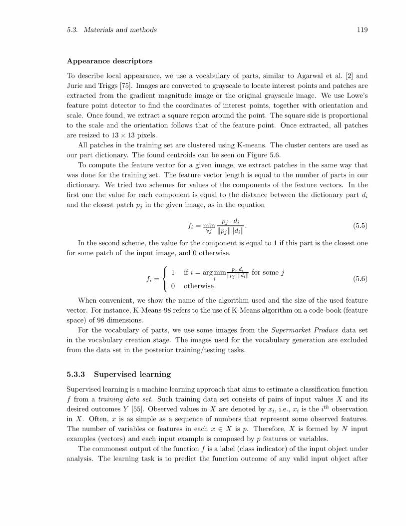
5.3. Materials and methods 119
Appearance descriptors
To describe local appearance, we use a vocabulary of parts, similar to Agarwal et al. [2] and
Jurie and Triggs [75]. Images are converted to grayscale to locate interest points and patches are
extracted from the gradient magnitude image or the original grayscale image. We use Lowe’s
feature point detector to find the coordinates of interest points, together with orientation and
scale. Once found, we extract a square region around the point. The square side is proportional
to the scale and the orientation follows that of the feature point. Once extracted, all patches
are resized to 13× 13 pixels.
All patches in the training set are clustered using K-means. The cluster centers are used as
our part dictionary. The found centroids can be seen on Figure 5.6.
To compute the feature vector for a given image, we extract patches in the same way that
was done for the training set. The feature vector length is equal to the number of parts in our
dictionary. We tried two schemes for values of the components of the feature vectors. In the
first one the value for each component is equal to the distance between the dictionary part di
and the closest patch pj in the given image, as in the equation
fi = min∀j
pj · di
‖pj‖‖di‖. (5.5)
In the second scheme, the value for the component is equal to 1 if this part is the closest one
for some patch of the input image, and 0 otherwise.
fi =
1 if i = arg mini
pj ·di
‖pj‖‖di‖for some j
0 otherwise(5.6)
When convenient, we show the name of the algorithm used and the size of the used feature
vector. For instance, K-Means-98 refers to the use of K-Means algorithm on a code-book (feature
space) of 98 dimensions.
For the vocabulary of parts, we use some images from the Supermarket Produce data set
in the vocabulary creation stage. The images used for the vocabulary generation are excluded
from the data set in the posterior training/testing tasks.
5.3.3 Supervised learning
Supervised learning is a machine learning approach that aims to estimate a classification function
f from a training data set. Such training data set consists of pairs of input values X and its
desired outcomes Y [55]. Observed values in X are denoted by xi, i.e., xi is the ith observation
in X. Often, x is as simple as a sequence of numbers that represent some observed features.
The number of variables or features in each x ∈ X is p. Therefore, X is formed by N input
examples (vectors) and each input example is composed by p features or variables.
The commonest output of the function f is a label (class indicator) of the input object under
analysis. The learning task is to predict the function outcome of any valid input object after

120 Chapter 5. Automatic Fruit and Vegetable Classification from Images
(a) Grayscale. (b) Gradients.
Figure 5.6: Dictionary of parts, clustered using K-means.
having seen a sufficient number of training examples.
In the literature, there are many different approaches for supervised learning such as Linear
Discriminant Analysis, Support Vector Machines, Classification Trees, and Neural Networks.
Linear Discriminant Analysis
Also known as Fisher discriminant, Linear Discriminant Analysis (LDA) consists of selecting
the components that maximize the between-class differences while minimizing the within-class
variability [16].
For the sake of simplicity, consider a two-class classification problem Y (-1 = a | +1 = b).
Let Xa be a set of examples belonging to the class a and Xb be a set of examples belonging to
class b in the training set. Consider the number of elements in Xa to be Na and the number of
elements in Xb to be Nb.
Let’s suppose that both classes a and b have a Gaussian distribution. Therefore, we can
define the within-class means as
µa =1
Na
∑
xi∈Xa
xi and µb =1
Nb
∑
xj∈Xb
xj. (5.7)
We define the between-class (a, b) means as
µ =1
Na + Nb
∑
x∈Xa∪Xb
x
. (5.8)

5.3. Materials and methods 121
We define the within-class scatter matrix Sw as
Sw = MaMTa + MbM
Tb , (5.9)
where the ith column of matrix Ma contains the difference (xai − µa). We can apply the same
procedure to Mb. The scatter matrix Sbet between the classes is
Sbet = Na(µa − µ)(µa − µ)T + Nb(µb − µ)(µb − µ)T . (5.10)
In order to maximize the between-class differences and to minimize the within-class variability
in one single dimension (1-D), it is enough to calculate the generalized eigenvalue-eigenvector ~e
of Sbet and Sw
Sbet~e = λSw~e.
With the generalized eigenvalue-eigenvector, we can project the samples to a linear subspace
and use a single threshold to perform the classification.
Support Vector Machine (SVM)
In the SVM model, we are looking for an optimal separating hyper-plane between two classes.
This is done maximizing the margin (minimal distance of an example to the decision surface).
When it is not possible to find a linear separator, we project the data into a higher space
using techniques known as kernels [16]. SVMs can be linear separable, linear non-separable and
non-linear.
In the linear separable SVMs, the points that lie on the hyper-plane satisfy the constraint
wtxi + b = 0, (5.11)
where w is the normal to the hyper-plane, b is the bias of the hyper-plane, |b|/‖w‖ is the
perpendicular distance from the origin to the hyper-plane and ‖.‖ is the Euclidean norm. To
find out w and maximize the margin, we can use Lagrangian multipliers
L(α) =N∑
i=1
αi −1
2
N∑
i=1
N∑
j=1
αiαjxtixjyiyj, (5.12)
where α is the positive Lagrangian multipliers, x are the samples of the X input vector and y
are the expected outputs. A solution to the linear separable classifier, if it exists, yields values
of αi. Using the αi values, we can calculate the normal to the hyperplane w
w =N∑
i=1
αixiyi. (5.13)
From w we can calculate the bias b of the separating hyperplane applying the Karush-Kuhn-
Tucker [16] condition
b =1
N
N∑
i=1
yi − wtxi. (5.14)
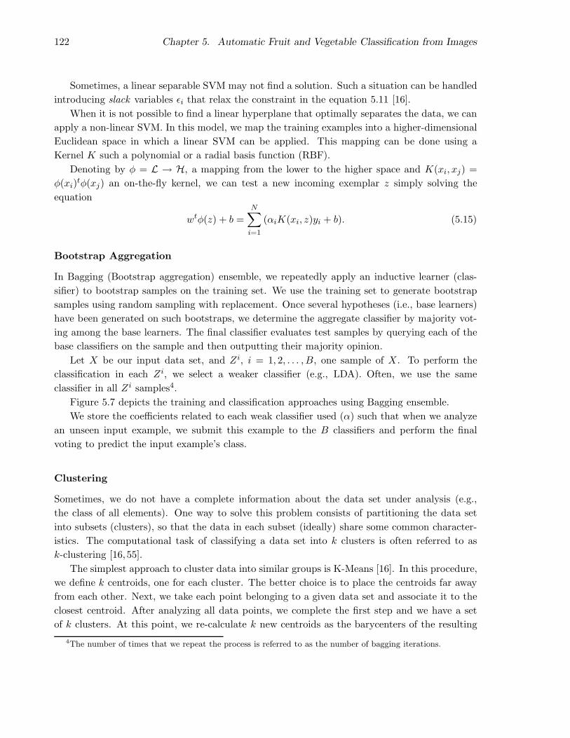
122 Chapter 5. Automatic Fruit and Vegetable Classification from Images
Sometimes, a linear separable SVM may not find a solution. Such a situation can be handled
introducing slack variables ǫi that relax the constraint in the equation 5.11 [16].
When it is not possible to find a linear hyperplane that optimally separates the data, we can
apply a non-linear SVM. In this model, we map the training examples into a higher-dimensional
Euclidean space in which a linear SVM can be applied. This mapping can be done using a
Kernel K such a polynomial or a radial basis function (RBF).
Denoting by φ = L → H, a mapping from the lower to the higher space and K(xi, xj) =
φ(xi)tφ(xj) an on-the-fly kernel, we can test a new incoming exemplar z simply solving the
equation
wtφ(z) + b =
N∑
i=1
(αiK(xi, z)yi + b). (5.15)
Bootstrap Aggregation
In Bagging (Bootstrap aggregation) ensemble, we repeatedly apply an inductive learner (clas-
sifier) to bootstrap samples on the training set. We use the training set to generate bootstrap
samples using random sampling with replacement. Once several hypotheses (i.e., base learners)
have been generated on such bootstraps, we determine the aggregate classifier by majority vot-
ing among the base learners. The final classifier evaluates test samples by querying each of the
base classifiers on the sample and then outputting their majority opinion.
Let X be our input data set, and Zi, i = 1, 2, . . . , B, one sample of X. To perform the
classification in each Zi, we select a weaker classifier (e.g., LDA). Often, we use the same
classifier in all Zi samples4.
Figure 5.7 depicts the training and classification approaches using Bagging ensemble.
We store the coefficients related to each weak classifier used (α) such that when we analyze
an unseen input example, we submit this example to the B classifiers and perform the final
voting to predict the input example’s class.
Clustering
Sometimes, we do not have a complete information about the data set under analysis (e.g.,
the class of all elements). One way to solve this problem consists of partitioning the data set
into subsets (clusters), so that the data in each subset (ideally) share some common character-
istics. The computational task of classifying a data set into k clusters is often referred to as
k-clustering [16,55].
The simplest approach to cluster data into similar groups is K-Means [16]. In this procedure,
we define k centroids, one for each cluster. The better choice is to place the centroids far away
from each other. Next, we take each point belonging to a given data set and associate it to the
closest centroid. After analyzing all data points, we complete the first step and we have a set
of k clusters. At this point, we re-calculate k new centroids as the barycenters of the resulting
4The number of times that we repeat the process is referred to as the number of bagging iterations.

5.4. Background subtraction 123
Training Classification
[x1, y1][x2, y2]
[xn, yn]
[x, y][x′
1, y′1]
[x′1, y
′1]
[x′1, y
′1]
[x′2, y
′2]
[x′2, y
′2]
[x′2, y
′2]
[x′n, y′n]
[x′n, y′n]
[x′n, y′n]
...
...
...
...
...
...
...
Z1
Z2
ZB
α1
α1
α2
α2
αBαB
Classifier1
Classifier2
ClassifierB
Voting
Sam
plin
g
with
repe
tition
fbag(x)
Figure 5.7: Training and classification using Bagging ensemble.
clusters from the previous step. With the k new centroids, we perform a new binding between
the same data set points and the closest new centroid. We repeat this process until we reach a
stabilization criterion.
5.4 Background subtraction
Background subtraction is a convenient and effective method for detecting foreground objects
in images with stationary background.
This task has been widely studied in the literature. Background subtraction techniques can
be seen as a two-object image segmentation and, often, need to cope with illumination variations
and sensor capturing artifacts such as blur. For our problem we also face specular reflections,
background clutter, shading and shadows.
For a real application in a supermarket, background subtraction needs to be fast, requiring
only fractions of a second to be performed.
In this paper, we tested several background subtraction techniques. After analyzing the cost
effectiveness of each one, we present a solution that gives us good solutions in less than a second.
In the following, we present some results for the different approaches we studied.
For the following experiments, we used a 2.1GHz machine with 2GB of RAM. No other
program was executed in parallel. We discovered that, for our problem, the best channel to per-
form the background subtraction is the S channel of HSV-stored images. This is understandable
given that the S channel is much less sensitive to lighting variations than any of the RGB color
channels [60]. Therefore, for all tests reported, we performed the segmentation in the S channel.
Figure 5.8 depicts results for four different approaches. Otsu background algorithm [124] is

124 Chapter 5. Automatic Fruit and Vegetable Classification from Images
the fastest tested approach requiring only 0.3 seconds to segment an input image of 640 × 480
pixels. However, as we see, it misses most of the produce under analysis. Meanshift [30] provides
a good image segmentation within 1.5 seconds in average. However, it requires the correct tuning
of parameters for different image classes. The affinity threshold for merging regions, also known
as bandwidth in Meanshift, is different for each image class and sometimes even within the same
class. Although, in general, the Normalized cuts [165] approach provided the best segmentation
results, it has a serious drawback for our problem. Given that the approach needs to calculate
the eigenvectors of the image, even for a reduced image (128×96 pixels), it requires ≈ 5 seconds
to perform the segmentation, not counting the image resizing operation.
Finally, K-Means is the approach that yields good segmentation results within acceptable
computing time. To analyze an image of 640 × 480, it requires 0.8 seconds for the whole
procedure described in Algorithm 6. We also tested Watershed transform [90] followed by some
morphological operations and the results are similar to Otsu’s algorithm.
(a) Original. (b) Otsu. (c) Meanshift. (d) Normalized Cuts.
(e) K-Means.
Figure 5.8: Background subtraction results for four different approaches.
In this sense, we chose the approach based on K-Means to perform the background subtrac-
tion and reduce most of the artifacts due to lighting variation conditions. Algorithm 6 presents
the complete procedure for this task.
Algorithm 6 Background subtraction based on K-MeansRequire: Input image I stored in HSV;1: Idown ← Down-sample the image to 25% of its original size using simple linear interpolation.2: Get the S channel of Idown and consider it as an 1-d vector V of pixel intensities.3: Perform Dbin = K-Means(V , k=2) ⊲ Sec. 5.3.34: Map M ← Dbin back to image space. For that just do a linear scan of Dbin.5: Mup ← Up-sample the generated binary map M back to the input image size.6: Close small holes on Mup using the Closing morphological operator with a disk structuring element
of radius 7 pixels.
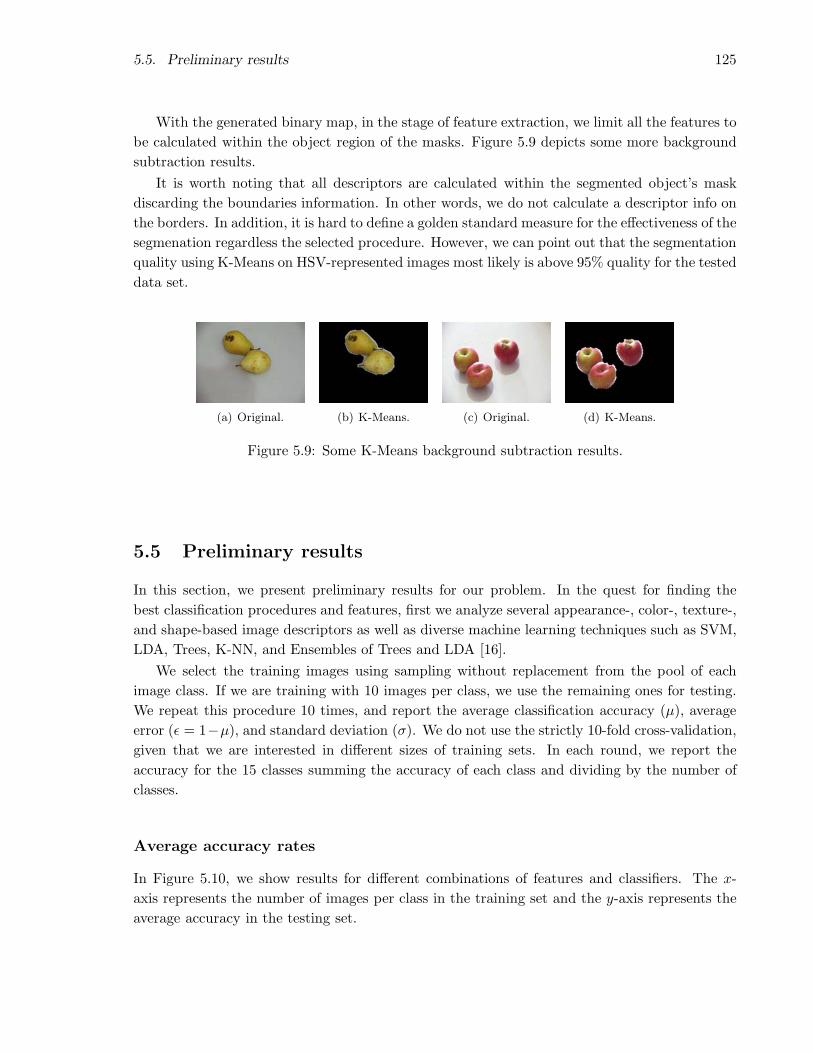
5.5. Preliminary results 125
With the generated binary map, in the stage of feature extraction, we limit all the features to
be calculated within the object region of the masks. Figure 5.9 depicts some more background
subtraction results.
It is worth noting that all descriptors are calculated within the segmented object’s mask
discarding the boundaries information. In other words, we do not calculate a descriptor info on
the borders. In addition, it is hard to define a golden standard measure for the effectiveness of the
segmenation regardless the selected procedure. However, we can point out that the segmentation
quality using K-Means on HSV-represented images most likely is above 95% quality for the tested
data set.
(a) Original. (b) K-Means. (c) Original. (d) K-Means.
Figure 5.9: Some K-Means background subtraction results.
5.5 Preliminary results
In this section, we present preliminary results for our problem. In the quest for finding the
best classification procedures and features, first we analyze several appearance-, color-, texture-,
and shape-based image descriptors as well as diverse machine learning techniques such as SVM,
LDA, Trees, K-NN, and Ensembles of Trees and LDA [16].
We select the training images using sampling without replacement from the pool of each
image class. If we are training with 10 images per class, we use the remaining ones for testing.
We repeat this procedure 10 times, and report the average classification accuracy (µ), average
error (ǫ = 1−µ), and standard deviation (σ). We do not use the strictly 10-fold cross-validation,
given that we are interested in different sizes of training sets. In each round, we report the
accuracy for the 15 classes summing the accuracy of each class and dividing by the number of
classes.
Average accuracy rates
In Figure 5.10, we show results for different combinations of features and classifiers. The x-
axis represents the number of images per class in the training set and the y-axis represents the
average accuracy in the testing set.

126 Chapter 5. Automatic Fruit and Vegetable Classification from Images
LDA−BICSVM−BICTree−BIC
BLDA−17−BICBAGG−17−BIC
KNN−3−BIC
Training examples per class
Acc
ura
cy(%
)
8 16 2430
32 40
40
48
50
56
60
64
70
80
90
100
(a) Feature: BIC
LDA−GCHSVM−GCHTree−GCH
BLDA−17−GCHBAGG−17−GCH
KNN−3−GCH
Training examples per class
Acc
ura
cy(%
)
8 16 2430
32 40
40
48
50
56
60
64
70
80
90
100
(b) Feature: GCH
LDA−CCVSVM−CCVTree−CCV
BLDA−17−CCVBAGG−17−CCV
KNN−3−CCV
Training examples per class
Acc
ura
cy(%
)
8 16 2430
32 40
40
48
50
56
60
64
70
80
90
100
(c) Feature: CCV
LDA−UnserSVM−UnserTree−Unser
BLDA−17−UnserBAGG−17−Unser
KNN−3−Unser
Training examples per class
Acc
ura
cy(%
)
8 16 2430
32 40
40
48
50
56
60
64
70
80
90
100
(d) Feature: Unser
SVM−Patches−98−GradientSVM−Patches−98−No−Gradient
SVM−Patches−98−Binary
Training examples per class
Acc
ura
cy(%
)
8 1620
24
25
30
32
35
40
40
45
48 56 64
(e) Feature: Appearance Patches
Figure 5.10: Average accuracy per class considering diverse classifiers and features.
5.5. Preliminary results 127
In this experiment, we see that Breiman’s decision Tree does not perform very well. One
possible explanation is that the descriptor data is not suitable for this kind of classifier. For
instance, the Unser descriptor feature vector is continuous and unbounded which naturally makes
decision trees unstable.
In this sense, the ensemble of trees (BAGG), with 17 iterations performs better than simple
decision Trees as far as it is more stable.
We also observe across the plots that LDA accuracy curves practically become flat for more
than 32 examples. When we use an ensemble of LDA (BLDA), we are performing random
sampling across the training data that makes a better use of the provided information in such
a way it can improve the classification. Therefore, as we observe in the plots, the ensemble
of LDA with 17 iterations performs better than straight LDA, Trees, or ensemble of Trees.
Complementing, the simple K-Nearest Neighbors here is as good as ensemble of Trees no matter
the descriptor. K-NN is also not well suited for unbounded and unrestricted data like Unser
descriptor (c.f., Fig. 5.10(d)). In particular, SVM is a classifier that performs well regardless the
used features.
As we can see, for this problem, BIC descriptor performs best yielding an accuracy ≈ 94%
for 32 examples per class in the training under SVM classifier.
Furthermore, a more complex approach such as the appearance descriptor for this particu-
lar problem does not yield a good classification accuracy, as Figure 5.10(e) depicts. We tested
three different approaches for the appearance-based descriptor in Figure 5.10(e). Two interest-
ing observations: (1) the approach based on patches with no gradient orientation is the only
tested feature which does not benefit from more examples in the training; and (2) the approach
based on patches with gradient orientation is the one which benefits more with more training
examples. This suggests us that with enough training it might provide much better results.
Notwithstanding, the training data is limited for the particular problem in this paper.
We believe that the appearance descriptor does not provide a significant classification accu-
racy given that the used patches do not represent well all the images classes we are trying to
classify. Further investigation must be done in this direction to validate the use of appearance
descriptor or any other similar model. However, one observation that pops up is that this model
requires more sophisticated training. Although, previous results in literature argue that it re-
quires less examples for training, we noted that it requires lots of good representative images to
create good appearance patches and accomplish such claims.
We can draw some important general conclusions when analyzing these results. First, it
is hard to solve a multi-class problem using just one feature descriptor. Hence feature fusion
becomes mandatory. Second, we see that the classifier results for different features are quite
different suggesting us that it would be worth also combining the classifiers each one tailored
and best-suited for a particular feature.
In spite of the fact that feature-level combination is not straightforward for multi-class prob-
lems, for binary problems this is a simple task. In this scenario, it is possible to combine different
classifiers and features by using classic rules such as and, or, max, sum, or min [16]. For multi-
class problems, this is more difficult given that one feature might point out to an outcome class

128 Chapter 5. Automatic Fruit and Vegetable Classification from Images
Ci and another feature might result the outcome class Cj, and even another one could result
Ck. With many different resulting classes for the same input example, it becomes difficult to
define a consistent policy to combine the selected features.
In this context, one approach sometimes used is to combine the feature vectors for different
features into a single and big feature vector. Although quite effective for some problems, this
approach can also yield unexpected classification results when not properly prepared. First,
in order to create the combined feature vector, we need to tackle the different nature of each
feature. Some can be well conditioned such as continuous and bounded variables, others can be
ill-conditioned for this combination such as categorical ones. In addition, some variables can be
continuous and unbounded. To put everything together, we need a well-suited normalization.
However, this normalization is not always possible or, sometimes, it leads to undesirable prop-
erties in the new generated feature vector such as equally weighting all the feature coefficients,
a property that in general we do not want.
When combining feature vectors this way, eventually we would need to cope with the curse
of dimensionality. Given that we add new features, we increase the number of dimensions which
then might require more training data.
Finally, if we want to add a new feature, we might need to redesign the normalization in
order to deal with all the aforementioned problems. In Section 5.6, we present a simple and
effective way to feature and classifier fusion that cope with most of the previously discussed
concerns.
5.6 Feature and classifier fusion
Our objective is to combine a set of features and the most appropriate classifier for each one in
such a way we improve the overall classification accuracy. Given that we do not want to face the
inherent problems of proper normalization and curse of dimensionality, we do not create a big
feature vector combining the selected features. Furthermore, doing that we would only perform
feature fusion and we would still be limited in doing the classifier fusion.
To accomplish our objective, we propose to cope with the multi-class problem as a set of
binary problems. In this context, we define a class binarization as a mapping of a multi-class
problem onto two-class problems (divide-and-conquer) and the subsequent combination of their
outcomes to derive the multi-class prediction. We refer to the binary classifiers as base learners.
Class binarization has been used in the literature to extend naturally binary classifiers to multi-
class and SVM is one example of this [5,38,115]. However, to our knowledge, this approach was
not used before for classifier and feature fusion.
In order to understand the class binarization, consider a problem with 3 classes. In this case,
a simple binarization consists in training three base learners, each one for two classes. In this
sense, we need O(N2) binary classifiers, where N is the number of classes.
We train the ijth binary classifier using the patterns of class i as positive and the patterns
of class j as negative examples. To obtain the final outcome we just calculate the minimum

5.6. Feature and classifier fusion 129
distance of the generated vector (binary outcomes) to the binary pattern representing each class.
Consider again a toy example with three classes as we show in Figure 5.11. In this example,
we have the classes: Triangles , Circles ©, and Squares 2. Clearly, one first feature we
can use to categorize elements of these classes can be based on shape. As we can see, we can
also use texture and color properties. To solve this problem, we train some binary classifiers
differentiating two classes at a time, such as ש, ×2, and ©×2. Also, we give each one
of our classes a unique identifier (e.g., = 〈+1, +1, 0〉).
Figure 5.11: Toy example for feature and classifier fusion.
When we receive an input example to classify, let’s say a triangle-shaped one, as we show
in the picture, we first apply our binary classifiers to verify if the input example is a triangle
or a circle based on shape, texture and color features. Each classifier will give us a binary
response. Let’s say we obtain the votes 〈+1, +1,−1〉 for the binary classifier ש. Thereafter,
we can use majority voting and select one response (+1 in this case, or ). Then we repeat
the procedure and test if the input example is a triangle or a square, again for each one of the

130 Chapter 5. Automatic Fruit and Vegetable Classification from Images
considered features. Finally, after performing the last test, we end up with a binary vector.
Then we calculate the minimum distance from this binary vector to each one of the class unique
IDs. In this example, the final answer is given by the minimum distance of
min dist(〈1, 1,−1〉, 〈1, 1, 0〉, 〈−1, 0, 1〉, 〈0,−1,−1〉. (5.16)
One aspect of this approach is that it requires more storage given that once we train the
binary classifiers we need to store their parameters. Given that we analyze more features we
need more space. With respect to running time, there is also a small increase given that we
need to test more binary classifiers to provide an outcome. However, many classifiers in our
daily-basis employ some sort of class binarization (e.g., SVM) and are considered fast. The
majority voting for each binary classifier and the distance calculation to the unique class IDs
are simple and efficient operations.
Although we require more storage and increase the classification time with respect to a
normal multi-class approach, there are some advantages using this approach:
1. By combining independent features, we have more confidence in a resulting outcome given
that it is calculated from the agreement of more than one single feature. Hence, we have
a simple error correcting mechanism that can withstand some misclassifications;
2. If we find some classes that are in confusion and are driving down our classification results,
we can design special and well-tuned binary classifiers and features to separate them;
3. We can easily point out if one feature is indeed helping the classification or not. This is
not straightforward with normal binding in a big feature vector;
4. The addition of new classes only require training for the new binary classifiers;
5. The addition of new features is simple and also just require partial training;
6. As we do not increase the size of any feature vector, we are less prone to the curse of
dimensionality not requiring more training examples when adding more features.
Finally, there is no requirement to combine the binary classifiers using all combinations of
two classes at a time. We can reduce storage requirements and speed up the classification itself
by selecting classes that are in confusion and designing specific binary classifiers to separate
them. The expectation in this case is that much less binary classifiers would be needed. In fact,
there is room for more research in this direction.
5.7 Fusion results
We have seen in Section 5.5 that it is hard to solve a complex problem such as the one in this
paper using just one feature descriptor. Therefore, we face the need for feature fusion to improve
classification. In addition, we also observed that some classifiers are better for some features
5.7. Fusion results 131
than others which suggests us that it would be worth also combining the classifiers, each one
tailored and best-suited for a particular feature. We also discussed that common feature fusion
approaches, although effective and powerful in some cases, require careful understanding of the
used features and their proper normalization. Furthermore, this kind of feature combination
increase the dimensionality of the feature vectors and may require more training examples. In
this context, we presented in Section 5.6 an alternative approach that allows us to combine
features and classifiers in a simple way.
In this section, we present results for our approach and show that the combined features
and classifiers indeed improve classification results when compared to the standalone features
and classifiers. In the following experiments, we report results showing the average error in
classification and we seek to minimize this error. Finally, we show that with the top first
responses we have less than 2% error in classification and with the top two we have less than
1%.
5.7.1 General fusion results
Figure 5.13 shows one example of the combination of the BIC, CCV, and Unser descriptors.
This combination is interesting given that, BIC is a descriptor that analyzes color and shape
in the sense that it codifies the object’s border and interior, CCV codifies the color connected
components and Unser accounts for the image’s textures.
In Figure 5.13, we see that the fusion works well regardless the classifier used. Consider
the SVM classifier, with 32 examples per class in the training, the fusion yields an average
error of ǫ = 3, 0% and standard deviation of σ = 0.43%. This is better than the best
standalone feature, BIC, that is ǫ = 4.2% and standard deviation of σ = 0.32%. Although
the absolute difference here seems small, it is about 3 standard deviations which means it is
statistical significant. In general, to reduce one percentual point in the average error when
the baseline accuracy is ≈ 95% is a hard problem. For LDA classifier, the fusion requires at
least 24 examples per class in the training to yield error reduction. Recall that we observed in
Section 5.5 that LDA curves become flat with more than 32 examples per class in the training
and adding more training data does yield better results. On the other hand, when combining
different features, LDA does benefit from more training and indeed results lower error rates
(ǫ = 3%, σ = 0.59%), 9.8 standard deviations better than LDA on the straight BIC feature.
In Figure 5.14, we switch the BIC descriptor to a simpler one with half of the dimensionality
(64-d). As we note, the results are comparable to the ones obtained with the fusion before. But
now, the fusion show even more power.

132 Chapter 5. Automatic Fruit and Vegetable Classification from Images
5.7.2 Top two responses
Figure 5.12 shows the results when we require the system to show the top 2 responses. In this
case, the system provides the user the two most probable classes for a given input example
considering the different classifiers and features used. Using SVM classifier and fusion of BIC,
GCH, and Unser features, with 32 examples per class in the training, the average error is
ǫ ≤ 1%.
SVM−Fusion (BIC, Unser, CCV) − Top 2SVM−Fusion (GCH, Unser, CCV) − Top 2SVM−Fusion (GCH, Unser, CCV) − Top 1SVM−Fusion (BIC, Unser, CCV) − Top 1
Training examples per class
Ave
rage
Err
or(%
)
0
2
4
6
8
8
12
14
16
16
18
24 32 48 56 64
10
40
Figure 5.12: Top one, and two responses for SVM classifier considering fusion.
Average error per class
One important aspect when dealing with classification is the average error, or its counterpart,
average expected accuracy per class. This information, shows which class of our data needs
more attention when solving the confusions. Figure 5.15 shows us the average expected error
for each one of our 15 classes. Clearly, we see that Fuji apple is one class that needs particular
attention. It yields the highest error when compared to the other classes. Another class the has
an interesting error behavior is Onions. After the error decreases when using up to 40 training
examples it becomes higher as the number of training examples increases.
This experiments shows that for some classes, it might be worth performing the training
with less examples. Indeed, this is possible when using our fusion approach, since we analyze
each pair of classes with a separate classifier.
Average time
The average time for the image descriptors feature extraction and classification using any of the
classifiers under our feature and classifier fusion approach still is less than 1 second. However, the
more examples in the training set the more time consuming are the combinations in the training
stage. For instance, to train a multi-class classifier using our approach with SVM classifier, 48

5.8. Conclusions and remarks 133
SVM−Fusion (BIC, Unser, CCV)SVM−BIC
SVM−UnserSVM−CCV
Training examples per class
Ave
rage
Err
or(%
)
0
5
8
10
15
16
20
24
25
30
32
35
40 48 56 64
(a) SVM classifier
LDA−Fusion (BIC, Unser, CCV)LDA−BIC
LDA−UnserLDA−CCV
Training examples per class
Ave
rage
Err
or(%
)
0
5
8
10
15
16
20
24
25
30
32
35
40 48 56 64
(b) LDA classifier
BLDA−3−Fusion (BIC, Unser, CCV)BLDA−17−BIC
BLDA−17−UnserBLDA−17−CCV
Training examples per class
Ave
rage
Err
or(%
)
0
5
8
10
15
16
20
24
25
30
32
35
40
40
45
48 56 64
(c) BLDA classifier
Tree−Fusion (BIC, Unser, CCV)Tree−BIC
Tree−UnserTree−CCV
Training examples per class
Ave
rage
Err
or(%
)
08
10
16
20
24
30
32 40
40
48
50
56
60
64
70
(d) Tree classifier
Figure 5.13: Average error results for fusion of BIC, CCV, and Unser features.
training examples per class, and the combination of the features BIC, CCV, and Unser, it is
necessary about one hour in one 2.1GHz machine with 2GB of RAM.
Finally, the use of complex appearance descriptors such as appearance part-based ones can
impact the training set without yielding significant improvements on the overall effectiveness of
the classification system.
5.8 Conclusions and remarks
To solve a complex problem such us the one in this paper using just one feature descriptor is a
difficult task. We discussed that although normal feature fusion is quite effective for some prob-
lems, it can yield unexpected classification results when not properly normalized and prepared.
Besides it has the drawback of increasing the dimensionality which might require more training
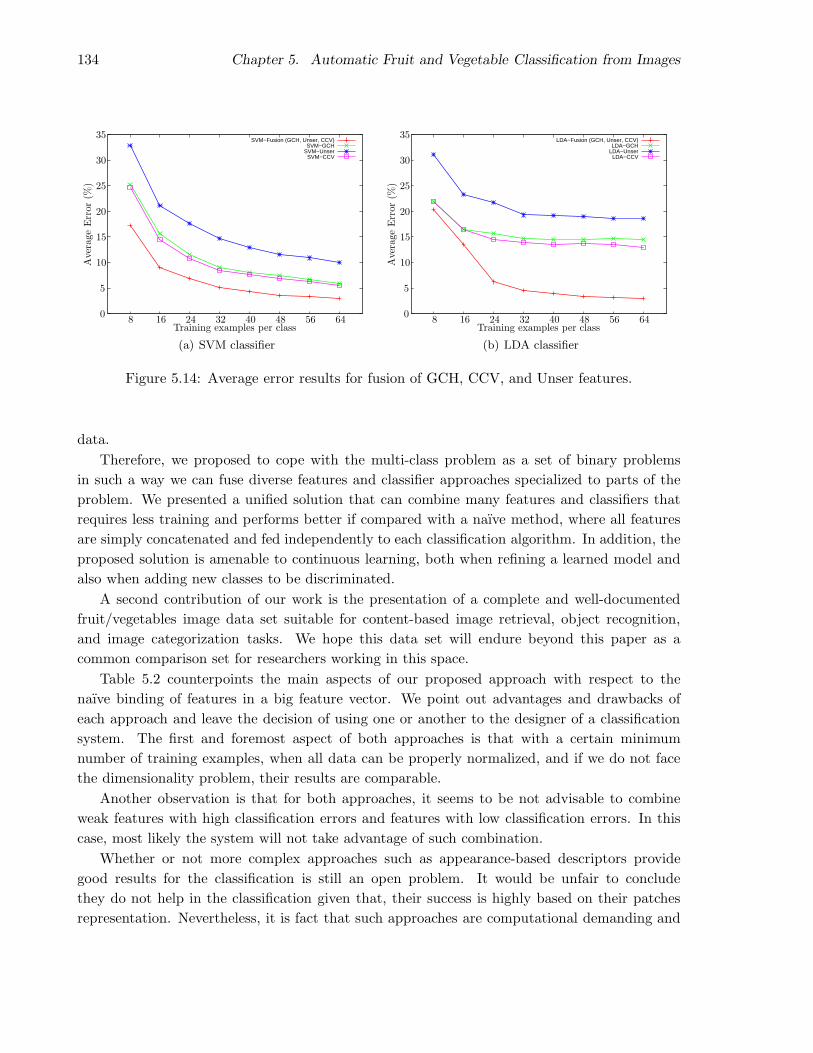
134 Chapter 5. Automatic Fruit and Vegetable Classification from Images
SVM−Fusion (GCH, Unser, CCV)SVM−GCH
SVM−UnserSVM−CCV
Training examples per class
Ave
rage
Err
or(%
)
0
5
8
10
15
16
20
24
25
30
32
35
40 48 56 64
(a) SVM classifier
LDA−Fusion (GCH, Unser, CCV)LDA−GCH
LDA−UnserLDA−CCV
Training examples per class
Ave
rage
Err
or(%
)
0
5
8
10
15
16
20
24
25
30
32
35
40 48 56 64
(b) LDA classifier
Figure 5.14: Average error results for fusion of GCH, CCV, and Unser features.
data.
Therefore, we proposed to cope with the multi-class problem as a set of binary problems
in such a way we can fuse diverse features and classifier approaches specialized to parts of the
problem. We presented a unified solution that can combine many features and classifiers that
requires less training and performs better if compared with a naıve method, where all features
are simply concatenated and fed independently to each classification algorithm. In addition, the
proposed solution is amenable to continuous learning, both when refining a learned model and
also when adding new classes to be discriminated.
A second contribution of our work is the presentation of a complete and well-documented
fruit/vegetables image data set suitable for content-based image retrieval, object recognition,
and image categorization tasks. We hope this data set will endure beyond this paper as a
common comparison set for researchers working in this space.
Table 5.2 counterpoints the main aspects of our proposed approach with respect to the
naıve binding of features in a big feature vector. We point out advantages and drawbacks of
each approach and leave the decision of using one or another to the designer of a classification
system. The first and foremost aspect of both approaches is that with a certain minimum
number of training examples, when all data can be properly normalized, and if we do not face
the dimensionality problem, their results are comparable.
Another observation is that for both approaches, it seems to be not advisable to combine
weak features with high classification errors and features with low classification errors. In this
case, most likely the system will not take advantage of such combination.
Whether or not more complex approaches such as appearance-based descriptors provide
good results for the classification is still an open problem. It would be unfair to conclude
they do not help in the classification given that, their success is highly based on their patches
representation. Nevertheless, it is fact that such approaches are computational demanding and

5.8. Conclusions and remarks 135
PlumAgata Potato
Asterix PotatoCashew
OnionKiwi
OrangeTaiti Lime
Training examples per class
Ave
rage
Err
or(%
)
0
5
8
10
15
16
20
24
25
30
32
35
40
40
48 56 64
Fuji AppleGranny Smith Apple
WatermelonHonneydew Melon
NectarineSpanish Pear
Diamond Peach
Training examples per class
Ave
rage
Err
or(%
)
0
5
8
10
15
16
20
24
25
30
32
35
40
40
48 56 64
Figure 5.15: Average error per class using fusion of the features BIC, CCV, and Unser, for anSVM classifier.
perhaps not advisable in some scenarios.
Further work include the improvement of the fruits/vegetables representative patches, and
the analysis of other appearance and texture image descriptors. Furthermore, we are interested
in the incorporation of spatial constraints among the local descriptors. In addition, we want
to create the conditions for a semi-supervised approach that leads us to continuous learning,
taking advantage of misclassified examples. In a semi-supervised scenario, the initial training
stage can be simplified requiring only a few examples for each analyzed class.
Acknowledgments
We are grateful to the people at our local fruits and vegetables distribution center for their
patience and help. In special, we thank Francisco Domingos of Agro Comercial Bella Vista
Ltda. Finally, we thank FAPESP (Grants 05/58103-3 and 07/52015-0) and CNPq (Grants
309254/2007-8 and 551007/2007-9) for their financial support.

136 Chapter 5. Automatic Fruit and Vegetable Classification from Images
Feature binding fusion Feature and classifier fusion using multi-class from binary
Short definition. It performs feature fusionby assembling together (binding) the diversefeature vectors resulting in a big feature vec-tor.
Short definition. It performs feature andclassifier fusion by considering the multi-classproblem as a set of binary problems and usingspecialized binary classifiers tuned for specificparts (divide-and-conquer).
Dimensionality problem. It might face thedimensionality problem when binding manyfeatures and creating a big feature vector.
Dimensionality problem. Less prone to thedimensionality problem in the feature fusion be-cause it uses each feature independently.
Selection of best features. Given that all thefeatures are addressed as just one feature, it ishard to point out which ones are more effectivein the fusion.
Selection of best features. It is straightfor-ward to point out which features are effectivein the fusion.
Training. New features and classes usually re-quire a complete new training.
Training. New features and classes would re-quire partial training. It only needs to trainnew binary classifiers for the new features andfor the new classes compared to the previousones.
In some cases, due to the dimensionality prob-lems, adding new features might require moretraining data.
Usually, more features do not require moretraining data.
Data normalization. It requires proper nor-malization of the data. Once new featuresare added, a new normalization and retrainingmust be performed.
Data normalization. It does not require spe-cial normalization given that each feature is in-dependently analyzed.
Testing. If the normalization is possible andproperly handled, the classification is easy.
Testing. The classification requires more stor-age for the classifier parameters. Furthermore,the classification itself is more time consuming.
Combining classifiers. The classifier is tiedto the features. It is not straightforward to usedifferent classifiers for different features.
Combining classifiers. Different classifiersand features can be combined with no restric-tions.
Table 5.2: Comparison between feature binding fusion and feature/classifier fusion using multi-class from binary.

Multi-classe a Partir de
Classificadores Binarios
Muitos problemas reais de reconhecimento e de classificacao frequentemente necessitam mapear
varias entradas em uma dentre centenas ou milhares de possıveis categorias.
Muitos pesquisadores tem proposto tecnicas efetivas para classificacao de duas classes nos
ultimos anos. No entanto, alguns classificadores poderosos tais como SVMs sao difıceis de
estender para o cenario multi-classe. Em tais casos, a abordagem mais comum e a de reduzir a
complexidade do problema multi-classe para pequenos e mais simples problemas binarios (dividir
para conquistar).
Ao utilizar classificadores binarios com algum criterio final de combinacao (reducao de com-
plexidade), muitas abordagens descritas na literatura partem do princıpio de que os classificado-
res binarios utilizados na classificacao sao independentes e aplicam um sistema de votacao como
polıtica final de combinacao. Entretanto, a hipotese da independencia nao e a melhor escolha
em todos os casos.
Nesse sentido, nos deparamos com um problema interessante: como tornar a utilizacao de
poderosos classificadores binarios no contexto multi-classe mais eficiente e eficaz?
No Capıtulo 6, introduzimos uma tecnica para combinacao de classificadores binarios (chama-
dos classificadores base) para a resolucao de problemas no contexto geral de multi-classificacao.
Nos denominamos a tecnica de Affine-Bayes. Finalmente, mostramos que nossa solucao torna
possıvel resolver problemas complexos tais como de 100 ou 1000 classes a partir da combinacao
de poucos, mas poderosos, classificadores binarios.
O Capıtulo 6 e uma compilacao de nosso trabalho submetido a IEEE Transactions on Pattern
Analysis and Machine Intelligence (TPAMI) e do artigo [150] no Intl. Conference on Computer
Vision Theory and Applications (VISAPP).
137

Chapter 6
From Binary to Multi-class: A
Bayesian Evolution
Abstract
Recently, there has been a lot of success in the development of effective binary classifiers. Al-
though many statistical classification techniques do have natural multi-class extensions, some,
such as the SVMs, do not. Therefore, it is important to know how to map the multi-class
problem into a set of simpler binary classification problems. In this paper, we introduce a new
Bayesian multi-class from binary reduction method: the Affine-Bayes Multi-class. First, we
introduce the concept of affine relations among the binary classifiers (dichotomies), and then we
present a principled way to find groups of highly correlated base learners. With that in hand, we
can learn the proper joint probabilities that allow us to predict the class. Finally, we present two
additional strategies: one to reduce the number of required dichotomies in the multi-class clas-
sification and the other to find new dichotomies in order to replace the less discriminative ones.
We can use these two new procedures iteratively to complement the base Affine-Bayes Multi-
class and boost the overall multi-class classification performance. We validate and compare our
approach to the literature in several open datasets that range from small (10 to 26 classes) to
large multi-class problems (1,000 classes) always using simple reproducible descriptors.
6.1 Introduction
Supervised learning is a Machine Learning strategy to create a prediction function from training
data. The task of the supervised learner is to predict the value of the function for any valid input
object after having seen a number of domain-related training examples [16]. Many supervised
learning techniques are conceived for binary classification [127]. However, a lot of real-world
139

140 Chapter 6. From Binary to Multi-class: A Bayesian Evolution
recognition and classification problems often require that we map inputs to one out of hundreds
or thousands of possible categories.
Several researchers have proposed effective approaches for binary classification in the last
years. Successful examples of such approaches are margin and linear classifiers, decision trees,
and ensembles. We can easily extend some of those techniques to multi-class problems (e.g.,
decision trees). However, we can not easily extend to multi-class some others powerful and
popular classifiers such as SVMs [31]. In such situations, the usual approach is to reduce the
multi-class problem complexity into multiple simpler binary classification problems. Binary
classifiers are more robust to the curse of dimensionality than multi-class approaches. Hence, it
is worth dealing with a larger number of binary problems.
A class binarization is a mapping of a multi-class problem onto several two-class problems
(divide-and-conquer) and the subsequent combination of their outcomes to derive the multi-class
prediction [130]. We refer to the binary classifiers as base learners or dichotomies.
There are many possible approaches to reduce multi-class to binary classification problems.
We can classify such approaches into three broad groups [145]: (1) One-vs-All (OVA), (2) One-
vs-One (OVO), and (3) Error Correcting Output Codes (ECOC). Also, the multi-class decom-
position into binary problems usually contains three main parts: (1) the ECOC matrix creation;
(2) the choice of the base learner; and (3) the decoding strategy.
Our focus here is on the creation of the ECOC matrix and on the decoding strategy. Although
we shall explain latter, for the creation of the ECOC matrix, it is important to choose a feasible
number of dichotomies to use. In general, the more base learners we use, the more complex is
the overall procedure. For the decoding strategy, it is essential to choose a deterministic strategy
robust to ties and errors in the dichotomies’ prediction.
In this paper, we introduce a brand new way to combine binary classifiers to perform large
multi-class classification. We present a new Bayesian treatment for the decoding strategy, the
Affine-Bayes Multi-class.
We propose a decoding approach based on the conditional probabilities of groups of high-
correlated binary classifiers. For that, we introduce the concept of affine relations among binary
classifiers and present a principled way to find groups of high correlated dichotomies.
Furthermore, we introduce two additional strategies: one to reduce the number of required
dichotomies in the multi-class classification and the other to find new dichotomies in order to
replace the less discriminative ones. These two new procedures are optional and can iteratively
complement the base Affine-Bayes Multi-class to boost the overall multi-class classification
performance.
Contemporary Vision and Pattern Recognition problems such as face recognition, finger-
printing identification, image categorization, and DNA sequencing often have an arbitrarily
large number of classes to cope with. Finding the right descriptor is just the first step to solve
a problem. Here, we show how to use a small number of simple, fast, and weak or strong base
learners to achieve good results, no matter the choice of the descriptor. This is a relevant issue
for large-scale classification problems.
We validate our approach using data sets from the UCI repository, NIST digits, Corel Photo

6.2. State-of-the-Art 141
Gallery, and the Amsterdam Library of Objects. We show that our approach provides better
results than all comparable approaches in the literature. Furthermore, we also compare our
approach to Passerini et al. [127], who proposed a Bayesian treatment for decoding assuming
independence among all binary classifiers.
We organize this paper as follows. In Section 6.2, we outline the state-of-the-art in multi-class
classification. In Section 6.3, we present our new Bayesian treatment for the decoding strategy:
the Affine-Bayes Multi-class as well as two new strategies to boost performance: the Shrinking
and Augmenting stages. Section 6.4 presents our experiments and results. In Section 6.5, we
draw conclusions and point out some future directions. Finally, in the Appendix, we provide a
table of symbols.
6.2 State-of-the-Art
Most of the existing literature addresses one or more of the three main parts of a multi-class de-
composition problem: (1) the ECOC matrix creation; (2) the dichotomies choice; and (3) the de-
coding.
In the following, let T be the team (set) of used dichotomies D in a multi-class problem, NT
be the size of T , and Nc be the number of classes1.
There are three broad groups for reducing multi-class to binary: One-vs-All, One-vs-One,
and Error Correcting Output Codes based methods [130].
1. One-vs-All (OVA). Here, we use NT = Nc = O(Nc) binary classifiers (dichotomies) [5,
28]. We train the ith classifier using all patterns of class i as positive (+1) examples and
the remaining class patterns as negative (−1) examples. We classify an input example x
to the class with the highest response.
2. One-vs-One (OVO). Here, we use NT =(Nc
2
)
= O(N2c ) binary classifiers. We train
the ijth dichotomy using all patterns of class i as positive and all patterns of class j as
negative examples. In this framework, there are many approaches to combine the obtained
outcomes such as voting, and decision directed acyclic graphs (DDAGs) [136].
3. Error Correcting Output Codes (ECOC). Proposed by Dietterich and Bakiri [38],
in this approach, we use a coding matrix M ∈ −1, 1Nc×NT to point out which classes to
train as positive and negative examples. Allwein et al. [4] have extended such approach and
proposed to use a coding matrix M ∈ −1, 0, 1Nc×NT . In this model, the jth column of
the matrix induces a partition of the classes into two meta-classes. An instance x belonging
to a class i is a positive instance for the jth dichotomy if and only if Mij = +1. If Mij = 0,
then it indicates that the ith class is not part of the training of the jth dichotomy. In this
framework, there are many approaches to combine the obtained outcomes such as voting,
Hamming and Euclidean distances, and loss-based functions [192].
1In the Appendix, we provide a table of symbols.
142 Chapter 6. From Binary to Multi-class: A Bayesian Evolution
When the dichotomies are margin-based learners, Allwein et al. [4] have showed the ad-
vantage and the theoretical bounds of using a loss-based function of the margin. Klau-
tau et al. [82] have extended such bounds to other functions.
It is worth noting that the asymptotic complexity O(Nc) refers to the number of required
dichotomies to perform a classification. It is not the only measure used to calculate the time
required for training and testing.
For training, we need to consider the number of training examples of each dichotomy, the
number of dichotomies used, and the complexity of each binary classifier with respect to the
number of minimum required operations to perform a classification. For testing, we need to
consider the number of dichotomies used and the complexity of each binary classifier.
In the case of OVO, the time complexity refers to the O(N2c ) dichotomies, each one requiring
positive and negative examples of the two classes being trained each time. For the testing, OVO
requires O(N2c ) binary classifications for each tested instance.
In the case of OVA, the time complexity refers to the O(Nc) dichotomies, each one requiring
positive examples of the class of interest and the negative examples of all the remaining classes.
For the testing, OVA requires O(Nc) binary classifications for each tested instance.
Pedrajas et al. [130] have proposed to combine the strategies of OVO and OVA. Although
the combination improves the overall multi-class effectiveness, the proposed approach uses
NT =(
Nc
2
)
+ Nc = O(N2c ) dichotomies in the training stage. Moreira and Mayoraz [112]
also developed a combination of different classifiers. They have considered the output of each
dichotomy as a probability of the pattern of belonging to a given class. This method requiresNc(Nc+1)
2 = O(N2c ) base learners. Athisos et al. [7] have proposed class embeddings to choose
the best dichotomies from a set of trained base learners.
Pujol et al. [145] have presented a heuristic method for learning ECOC matrices based on a
hierarchical partition of the class space that maximizes a discriminative criterion. The proposed
technique finds the potentially best Nc − 1 = O(Nc) dichotomies to the classification.
Crammer and Singer [33] have proven that the problem of finding optimal discrete codes is
NP-complete. Hence, Pujol et al. have used a heuristic solution for finding the best candidate
dichotomies. Even such solution is computationally expensive, and the authors only report
results for Nc ≤ 28.
Takenouchi and Ishii [173] have used the information transmission theory to combine
ECOC dichotomies. The authors use the full coding matrix M for the dichotomies, i.e.,
NT = 3Nc−2Nc+1+12 = O(3Nc) dichotomies. The authors only report results for Nc ≤ 7
classes.
Young et al. [195] have used dynamic programming to design an one-class-at-a-time removal
sequence planning method for multi-class decomposition. Although their approach only requires
NT = Nc − 1 dichotomies in the testing phase, the removal policy in the training phase is
expensive. The removal sequence for a problem with Nc classes is formulated as a multi-stage
decision-making problem and requires Nc−2 classification stages. In the first stage, the method
uses Nc dichotomies. In each one of the Nc − 3 remaining stages, the method uses Nc(Nc−1)2

6.3. Affine-Bayes Multi-class 143
dichotomies. Therefore, the total number of required base learners are N3c −4N2
c +5Nc
2 = O(N3c ).
Passerini et al. [127] have introduced a decoding function that combines the margins through
an estimation of their class conditional probabilities. The authors have assumed that all base
learners are independent and solved the problem using a Naıve Bayes approach. Their solution
works regardless of the number of selected dichotomies and can be associated with each one of
the previous approaches.
6.3 Affine-Bayes Multi-class
In this section, we present our new Bayesian treatment for the decoding strategy: the Affine-
Bayes Multi-class. We propose a decoding approach based on the conditional probabilities of
groups of affine binary classifiers. For that, we introduce the concept of affine relations among
binary classifiers, and present a principled way to find groups of high correlated dichotomies.
Finally, we present two additional strategies: one to reduce the number of required dichotomies
in the multi-class classification and the other to find new dichotomies in order to replace the less
discriminative ones. We can use these two new procedures iteratively to complement the base
Affine-Bayes Multi-class to boost the overall multi-class classification performance.
To classify an input, we use a team of trained base learners T . We call OT a realization of
T . Each element of T is a binary classifier (dichotomy) and produces an output ∈ −1, +1.Given an input element x to classify, a realization OT contains the information to determine the
class of x. In other words, P (y = ci|x) = P (y = ci|OT ).
However, we do not have the probability P (y = ci | OT ). From Bayes theorem,
P (y = ci|OT ) =P (OT |y = ci)P (y = ci)
P (OT )
∝ P (OT |y = ci)P (y = ci) (6.1)
P (OT ) is just a normalizing factor and it is suppressed.
Previous approaches have solved the above model by considering the independence of the
dichotomies in the team T [127]. If we consider independence among all dichotomies, the model
in Equation 6.1 becomes
P (y = ci|OT ) ∝∏
t ∈ T
P (OtT |y = ci)P (y = ci), (6.2)
and the class of the input x is given by
cl(x) = arg maxi
∏
t ∈ T
P (OtT |y = ci)P (y = ci). (6.3)
Although the independence assumption simplifies the model, it comes with limitations and it
is not the best choice in all cases [114]. In general, it is quite difficult to handle independence
without using smoothing functions to deal with numerical instabilities when the number of terms

144 Chapter 6. From Binary to Multi-class: A Bayesian Evolution
in the series is too large. In such cases, it is necessary to find a suitable density distribution to
describe the data, making the solution more complex.
We relax the assumption of independence among all binary classifiers. When two of these
dichotomies have a lot in common, it would be unwise to threat their results as independent
random variables (RVs). In our approach, we find groups of affine classifiers (high correlated
dichotomies) and represent their outcomes as dependent RVs, using a single conditional proba-
bility table (CPT) as an underlying distribution model. Each group then has its own CPT, and
we combine the groups as if they are independent from each other — to avoid a dimensionality
explosion.
Our technique is a Bayesian-Network-inspired approach for RV estimation. We decide the
RV that represents the class based on the RVs that represent the outcomes of the dichotomies.
We model the multi-class classification problem conditioned to groups of affine dichotomies
GD. The model in Equation 6.1 becomes
P (y = ci|OT ,GD) ∝ P (OT ,GD|y = ci)P (y = ci). (6.4)
We assume independence only among the groups of affine dichotomies gi ∈ GD. Therefore, the
class of an input x is given by
cl(x) = arg maxj
∏
gi ∈ GD
P (Ogi
T , gi|y = cj)P (y = cj). (6.5)
To find the groups of affine classifiers GD, we define an affinity matrix A among the classifiers.
The affinity matrix measures how affine are two dichotomies when classifying a set of training
examples X. In Section 6.3.1, we show how to create the affinity matrix A. After calculating the
affinity matrix A, we use a clustering algorithm to find the groups of correlated binary classifiers
in A. In Section 6.3.2, we show how to find the groups of affine dichotomies from an affinity
matrix A.
The groups of affine classifiers can contain classifiers that do not contribute significantly to
the overall classification. Therefore, we can deploy a procedure to identify the less important
dichotomies within an affine group and eliminate them.
With this shrinking stage, we can have two different objectives. On one hand, we might
want just to reduce the number of required dichotomies to perform the multi-class classification
and hence speed-up the overall process and make robust CPTs estimations. On the other hand,
we might want to eliminate less discriminative classifiers in order to replace them with more
powerful ones.
In Section 6.3.3, we show a consistent approach to eliminate the less important dichotomies
within an affine group. In addition, in Section 6.3.4, we introduce a simple idea to find di-
chotomies to replace the ones tagged as less discriminative in the Shrinking stage.
We can apply the Shrinking and Augmenting procedures iteratively until a convergence
criterion is satisfied. These two procedures are very fast since most of the information they need
is already calculated during the earlier training.
6.3. Affine-Bayes Multi-class 145
In Algorithm 7, we present the main steps of our model for multi-class classification. In
line 1, we divide the training data into five parts and use four parts to train the dichotomies and
one part to validate the trained dichotomies and to construct the conditional probability tables2.
In lines 3–6, we train and validate each dichotomy using a selected method. The method can
be any binary classifier such as LDA, or SVM.
Each dichotomy produces an output ∈ −1, +1 for each input x. In line 8, O contains all
realizations of the available dichotomies for the input data X ′. In lines 10 and 11, we find groups
of affine dichotomies using the realization Oi.
Using the information of groups of affine dichotomies, in line 12, we create a CPT for each
affine group. These CPTs provide the joint probabilities of a realization OT and the affine
groups gi ⊂ GD when testing an unseen input data x.
In line 13, our approach verifies if the user wants to find the less discriminative dichotomies
and replace them with better ones iteratively. If so, in line 14, we perform the shrinking stage
in order to tag the best dichotomies in the multi-class process.
In line 15, we use the error calculated in the training to find new dichotomies. In line 16, we
train the new dichotomies found in line 15. Note that in each iteration there are only a few of
them.
Afterwards, in line 17, we update the affinity matrix A to consider only the best dichotomies
tagged in the shrinking stage and, naturally, the new ones produced by the augmenting pro-
cedure. We also update the realizations Oi and the conditional probabilities accordingly. In
line 18, we perform clustering on the affinity matrix and find the updated groups of representa-
tive dichotomies GD′.
In line 19, we repeat lines 14–18 until a convergence criterion is satisfied. In our case, if
the training error produced by the updated team of classifiers is bigger than the error of the
previous step, we stop the iteration and discard the proposed augmented dichotomies. This is a
simple criterion and, as we show in the experiments, it yields good results.
If the user does not want to iteratively find the dichotomies, she might be interested in
the reduced set of dichotomies. Therefore, line 20 finds the best dichotomies within the affine
groups. This information can be used in the testing phase, for instance, simply to reduce the
number of used dichotomies.
6.3.1 Affinity matrix A
Given a training data set X, we introduce a metric to find the affinity between two dichotomies
realizations Di, Dj whose outputs ∈ −1, +1
Ai,j =1
N
∣
∣
∣
∣
∣
∑
∀ x ∈ X
Di(x)Dj(x)
∣
∣
∣
∣
∣
,∀ Di and Dj ∈ T . (6.6)
2The cross-validation is not a required step to our approach. We perform cross-validation in order to providefair results across the data sets.
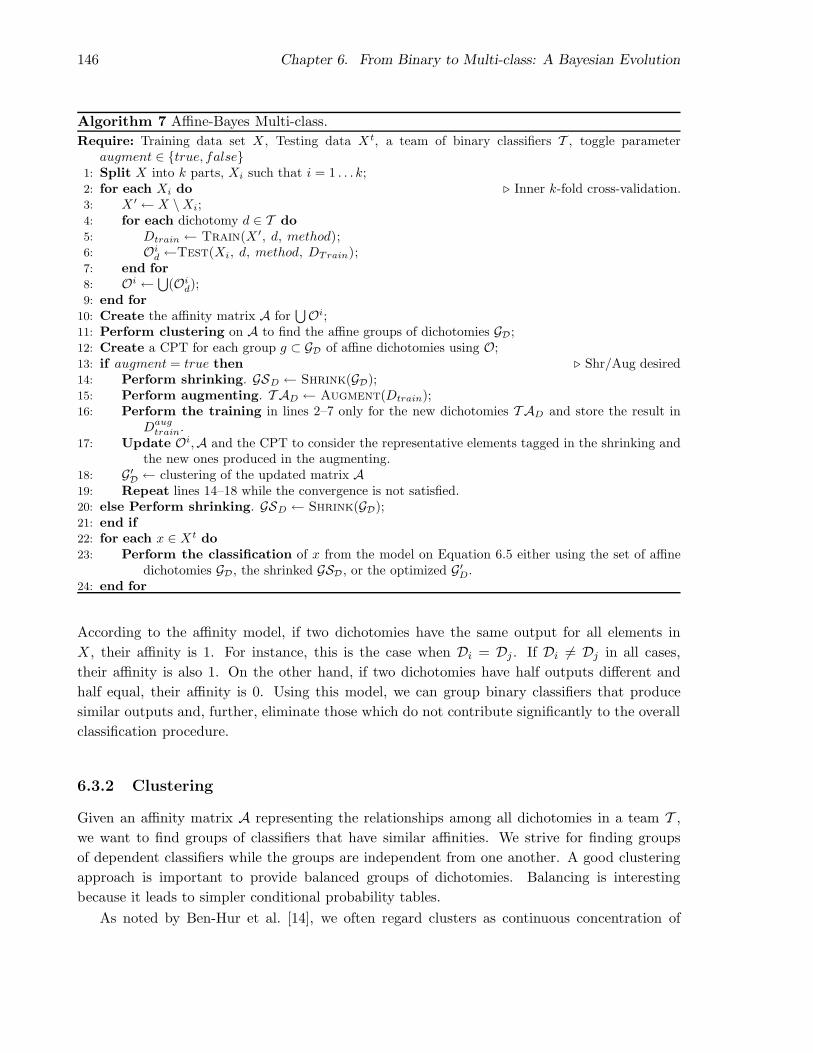
146 Chapter 6. From Binary to Multi-class: A Bayesian Evolution
Algorithm 7 Affine-Bayes Multi-class.
Require: Training data set X , Testing data Xt, a team of binary classifiers T , toggle parameteraugment ∈ true, false
1: Split X into k parts, Xi such that i = 1 . . . k;2: for each Xi do ⊲ Inner k-fold cross-validation.3: X ′ ← X \Xi;4: for each dichotomy d ∈ T do5: Dtrain ← Train(X ′, d, method);6: Oi
d ←Test(Xi, d, method, DTrain);7: end for8: Oi ← ⋃
(Oid);
9: end for10: Create the affinity matrix A for
⋃
Oi;11: Perform clustering on A to find the affine groups of dichotomies GD;12: Create a CPT for each group g ⊂ GD of affine dichotomies using O;13: if augment = true then ⊲ Shr/Aug desired14: Perform shrinking. GSD ← Shrink(GD);15: Perform augmenting. T AD ← Augment(Dtrain);16: Perform the training in lines 2–7 only for the new dichotomies T AD and store the result in
Daugtrain.
17: Update Oi,A and the CPT to consider the representative elements tagged in the shrinking andthe new ones produced in the augmenting.
18: G′D ← clustering of the updated matrix A19: Repeat lines 14–18 while the convergence is not satisfied.20: else Perform shrinking. GSD ← Shrink(GD);21: end if22: for each x ∈ Xt do23: Perform the classification of x from the model on Equation 6.5 either using the set of affine
dichotomies GD, the shrinked GSD , or the optimized G′D.24: end for
According to the affinity model, if two dichotomies have the same output for all elements in
X, their affinity is 1. For instance, this is the case when Di = Dj . If Di 6= Dj in all cases,
their affinity is also 1. On the other hand, if two dichotomies have half outputs different and
half equal, their affinity is 0. Using this model, we can group binary classifiers that produce
similar outputs and, further, eliminate those which do not contribute significantly to the overall
classification procedure.
6.3.2 Clustering
Given an affinity matrix A representing the relationships among all dichotomies in a team T ,
we want to find groups of classifiers that have similar affinities. We strive for finding groups
of dependent classifiers while the groups are independent from one another. A good clustering
approach is important to provide balanced groups of dichotomies. Balancing is interesting
because it leads to simpler conditional probability tables.
As noted by Ben-Hur et al. [14], we often regard clusters as continuous concentration of
6.3. Affine-Bayes Multi-class 147
data points. Two points belong to a cluster if they are close to each other, or if they are well
connected by paths of short “hops” over other points. The more we have such paths, the higher
are the chances the points belong to a cluster [47]. In this sense, Fisher and Poland [47], have
introduced a spectral clustering approach which we use in this paper. Instead of considering
two points similar if they are connected by a high-weight edge, the authors propose assign them
a high correlation if the overall graph conductivity between them is high. These considerations
exhibit an analogy to electrical networks: the conductivity between two nodes depends not only
on the conductivity of the direct path between them, but also on other indirect paths.
To find the conductivity for any two points xp and xq, we first solve the system of linear
equations:
Gϕ = η, (6.7)
where G is a matrix constructed from the original affinity matrix A:
G(p, q)=
for p = 1:
1 for q = 1
0 otherwise
otherwise:
∑
k6=pA(p, q) for p = q
−A(p, q) otherwise
(6.8)
and η is the vector representing points for which the conductivity is computed:
η(k) =
−1 for k = p and p > 1
1 for k = q
0 otherwise
(6.9)
Then the conductivity between xp and xq, p < q, due to the way η is constructed, is given by
C(p, q) =(
G−1(p, p) + G−1(q, q)−G−1(p, q)−G−1(q, p))−1
. (6.10)
Due to symmetry, C(p, q) = C(q, p) and it is necessary to compute G−1 only once.
The conductivity matrix C can be computed in O(N2) time. After building the conductivity
matrix from A, we can perform the clustering using any simple cluster method such as klines as
proposed in [47]. Although Fisher and Poland’s algorithm [47] has provided very good results for
our problem, we also have observed similar results using a simpler, yet effective, approach with
a greedy algorithm for finding the dependent groups of dichotomies from the affinity matrix.
In the greedy clustering approach, first we find the dichotomy with the highest affinity sum
with respect to all its neighbors (row with highest sum inA). After that, we select the neighbors
with affinity greater or equal than a threshold t. Next, we check if each dichotomy in the group
is affine to the others and select those satisfying this requirement. This procedure results the
first affine group. Afterwards, we remove the selected dichotomies from the main team T and
repeat the process until we analyze all available dichotomies. Throughout experiments, we have
found that t = 0.6 is a good threshold.

148 Chapter 6. From Binary to Multi-class: A Bayesian Evolution
6.3.3 Shrinking
Sometimes, when modeling a problem using conditional probabilities, we have to deal with large
conditional probability tables which can lead to over-fitting. One approach to cope with this
problem is to suppose independence among all dichotomies which results in the smallest possible
CPT. However, as we show in this paper, this approach limits the representative power of the
Bayes approach. In the following, we show an alternative approach.
In the shrinking stage, we want to find the dichotomies within a group that are more relevant
for the overall multi-class classification. For that, we find the accumulative entropy of each
classifier within a group from the examples in the training data X. The higher the accumulative
entropy, the more representative is a specific dichotomy. Let hij be the accumulative entropy
for the classifier j within a group of affine dichotomies i. We define hij as
hij =∑
c∈CL
∑
x∈X
(
pxc log2(p
xc)+(1− px
c) log2 (1− pxc))
(6.11)
where pxc = P (y = c | x, gj
i ,Og
ji
x ), gji is the jth dichotomy within the affine group gi, O
gji
x is
its realization for the input x, and c ∈ CL the available class labels.
We choose the classifiers with the highest cumulative entropy to select the best classifiers
within an affine group. We have found in the experiments, that selecting 60% of the classifiers
is a good tradeoff between multi-class overall effectiveness and efficiency. One could use another
cutting criterion, such as the maximum CPT size. It is worth noting that this procedure is very
fast once we already have the required probabilities stored in the previously computed CPTs.
Hence, we do not need to scan the data to perform it.
During the training phase, our approach finds the affine groups of binary classifiers and tags
the most relevant dichotomies within each group. On one hand, this information can be used
in association with the Augmenting step (c.f., Sec. 6.3.4) that finds new substitutes for the non-
selected dichotomies. Both procedures, Shrinking and Augmenting can be performed until a
convergence criterion is satisfied. On the other hand, if no optimization for finding replacements
for the dichotomies is intended, the selected group of dichotomies can be used in the testing
phase simply to reduce the number of required classifiers in the multi-class task.
In summary, with our solution, we measure the affinity on the training data to learn the
binary classifiers relationship and decision surface. It is a simple and fast way to estimate the
distribution. Sometimes, a dichotomy may be in the team because it is critical for discriminating
between two particular classes. If so, it is unlikely it will share a group of high-correlated
classifiers because it would require this dichotomy to be high-correlated with all dichotomies in
such group. We have performed some experiments to test that and, in all tested cases, such
dichotomies specific for rare classes are kept in the final pool of dichotomies.
6.3.4 Augmenting
As we showed in Section 6.3.3, we are able to find and tag the dichotomies that are more
relevant for the overall multi-class performance with a simple approach. This leads us to the

6.3. Affine-Bayes Multi-class 149
natural consequence of finding new dichotomies to replace the ones that are less discriminative.
For this intent, in the augmenting stage, we want to find new dichotomies (rather than simple
random choice) to replace the less representative ones eliminated in the shrinking stage in order
to improve the overall multi-class performance.
To perform the augmenting, we use the confusion matrix generated in the training stage.
From such confusion matrix, we are able to point out the classes that are in more confusion
with each other. We use such information to build a representation of the confusions through
hierarchical clustering in order to determine the ones that need urgent dichotomies to solve them.
Afterwards, we sort the clusters according to the sum of the number of confusions normalized
by by the number of edges connecting the elements in that cluster excluding the self-references.
For each cluster, in order, we apply normalized cuts [165] to find the cut that maximizes the
separability of the cluster and, therefore, its confusion.
We summarize these procedures in Algorithm 8.
Algorithm 8 Augmenting procedure for Affine-Bayes.Require: A confusion matrix C already calculated in the training stage, and the number of dichotomies
n to generate1: Set the diagonal elements of C to zero2: Cij ← 1− Cij/
∑
i,j Cij ∀Cij ∈ C ⊲ Normalizing C3: H ← hierarchical clustering of C using, for instance, the simple Agnes [78] algorithm.4: Sort H according to the sum of the confusions of each group hi ⊆ H normalized by the number of
edges connecting the elements in the group hi excluding the self-references.5: for each group hi ⊆ H do6: d← normalized cuts of hi
7: TA ← TA ∪ d8: end for9: TAS ← the top n dichotomies ⊆ TA
10: Return TAS
In order to illustrate the augmenting process, let’s consider a step-by-step example. Let
C be a confusion matrix for a multi-class problem with five classes as we show in Table 6.1.
Here, we already set the diagonal of C to zero. This is required because we want to find the
classes that are in confusion and the diagonal represents the correct classifications rather than
the mis-classifications.
C1 C2 C3 C4 C5
C1 0 0 22 13 2C2 0 0 48 26 2C3 22 48 0 37 31C4 13 26 37 0 1C5 2 2 31 1 0
Table 6.1: An example of a confusion matrix C.
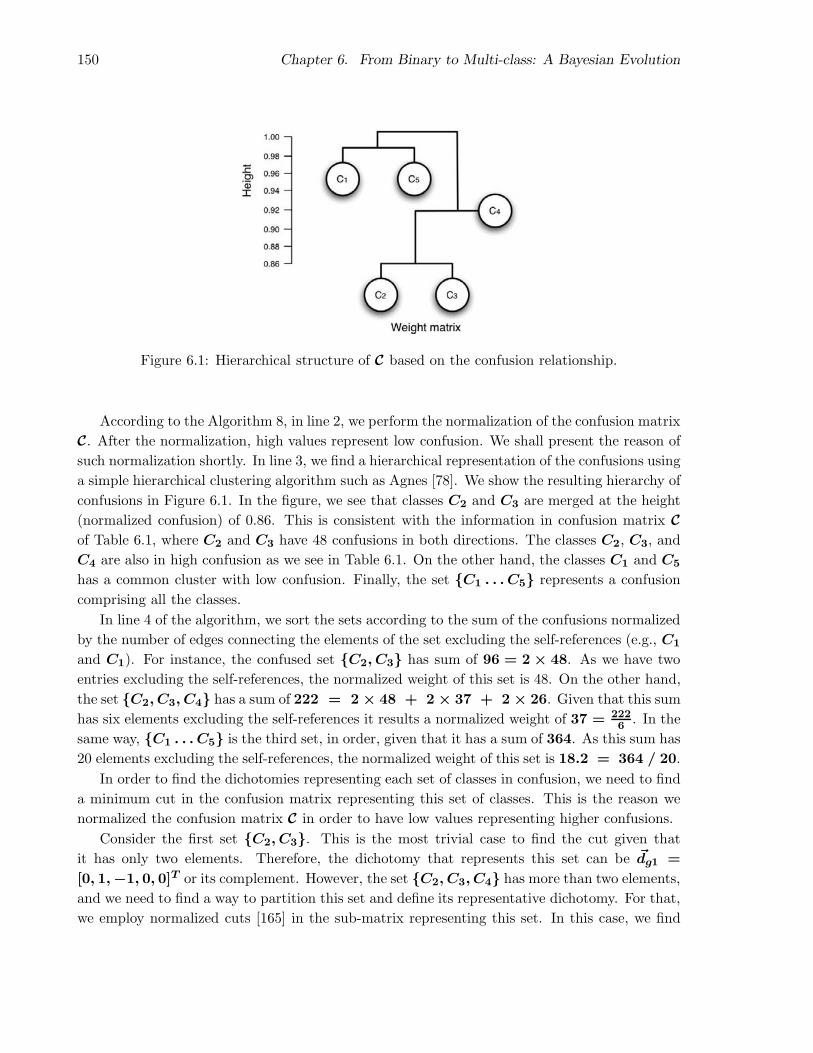
150 Chapter 6. From Binary to Multi-class: A Bayesian Evolution
Figure 6.1: Hierarchical structure of C based on the confusion relationship.
According to the Algorithm 8, in line 2, we perform the normalization of the confusion matrix
C. After the normalization, high values represent low confusion. We shall present the reason of
such normalization shortly. In line 3, we find a hierarchical representation of the confusions using
a simple hierarchical clustering algorithm such as Agnes [78]. We show the resulting hierarchy of
confusions in Figure 6.1. In the figure, we see that classes C2 and C3 are merged at the height
(normalized confusion) of 0.86. This is consistent with the information in confusion matrix C
of Table 6.1, where C2 and C3 have 48 confusions in both directions. The classes C2, C3, and
C4 are also in high confusion as we see in Table 6.1. On the other hand, the classes C1 and C5
has a common cluster with low confusion. Finally, the set C1 . . . C5 represents a confusion
comprising all the classes.
In line 4 of the algorithm, we sort the sets according to the sum of the confusions normalized
by the number of edges connecting the elements of the set excluding the self-references (e.g., C1
and C1). For instance, the confused set C2, C3 has sum of 96 = 2× 48. As we have two
entries excluding the self-references, the normalized weight of this set is 48. On the other hand,
the set C2, C3, C4 has a sum of 222 = 2× 48 + 2× 37 + 2× 26. Given that this sum
has six elements excluding the self-references it results a normalized weight of 37 = 222
6. In the
same way, C1 . . . C5 is the third set, in order, given that it has a sum of 364. As this sum has
20 elements excluding the self-references, the normalized weight of this set is 18.2 = 364 / 20.
In order to find the dichotomies representing each set of classes in confusion, we need to find
a minimum cut in the confusion matrix representing this set of classes. This is the reason we
normalized the confusion matrix C in order to have low values representing higher confusions.
Consider the first set C2, C3. This is the most trivial case to find the cut given that
it has only two elements. Therefore, the dichotomy that represents this set can be ~dg1 =
[0, 1,−1, 0, 0]T or its complement. However, the set C2, C3, C4 has more than two elements,
and we need to find a way to partition this set and define its representative dichotomy. For that,
we employ normalized cuts [165] in the sub-matrix representing this set. In this case, we find

6.4. Experiments and Results 151
the best cut to be between C2, C4 and C3. Therefore, the dichotomy that represents this
set can be ~dg2 = [0, 1,−1, 1, 0]T or its complement. Recall that such dichotomy means that
we are interested in solving the confusion among classes C2, C3, and C4, designing a binary
classifier specialized in separating elements from the classes C2, and C4 from elements of the
class C3 and disregarding the rest.
6.4 Experiments and Results
In this section, we compare our Affine-Bayes Multi-class approach to: OVO, OVA, and
ECOC approaches based on distances decoding strategies. We also compare our approach to
Passerini et al. [127], who have proposed a Bayesian treatment for decoding assuming indepen-
dence among all binary classifiers. For our Affine-Bayes Multi-class, we present three different
results: one for normal Affine-Bayes (AB), one for Affine-Bayes and one stage of Shrinking
(ABS), and finally, one with the iterative Shrinking-Augmenting (AB-OPT).
We validate our approach using two scenarios. In the first scenario, we use data sets with a
relative small number of classes (Nc < 30). For that, we use several UCI3, and one NIST4 data
sets. In the second scenario, we have considered three large-scale multi-class applications: one
for the Corel Photo Gallery (Corel)5 data set, one for the Australian Sign Language (Auslan)6,
and one for the Amsterdam Library of Objects (ALOI)7. Table 6.2 presents the main properties
of each data set we have used in the validation. Recall that, Nc is the number of classes, Nd if
the number of features, and N is the number of instances.
Data set Source Nc Nd N
Pendigits UCI 10 16 10,992Mnist digits NIST 10 785 10,000Vowel UCI 11 10 990Isolet UCI 26 617 7,797Letter-2 UCI 26 16 20,000
Auslan Auslan 95 128 2,565Corel Corel 200 128 20,000ALOI ALOI 1,000 128 108,000
Table 6.2: Data sets’ summary. For the Auslan data set, we perform a dimensionality reductionto 128 features.
In the ECOC-based experiments, we have selected 10 random coding matrices. For each
coding matrix, we perform 5-fold cross validation. For each cross-validation fold, we perform a
5-fold cross validation on the training set to estimate the CPTs. In all experiments, we have
3http://mlearn.ics.uci.edu/MLRepository.html
4http://yann.lecun.com/exdb/mnist/
5http://www.corel.com
6http://mlearn.ics.uci.edu/MLRepository.html
7http://www.science.uva.nl/~aloi/

152 Chapter 6. From Binary to Multi-class: A Bayesian Evolution
used both Linear Discriminant Analysis (LDA) and Support Vector Machines (SVMs) [16] as
base learners (examples of a week and a strong classifiers). For the clustering stage in our
Affine-Bayes Multi-class solution, we report results using Fisher and Poland technique, as we
showed in Section 6.3.2.
6.4.1 Scenario 1 (10 to 26 classes)
In Figures 6.2–6.4, we compare Affine-Bayes (AB) to ECOC based on Hamming decoding
(ECOC), One-vs-One (OVO), One-vs-All (OVA), and Passerini’s approach (PASSERINI) [127].
We show the One-vs-All (OVA) as the baseline and not as a function of the number of used
base-leaners. In this experiment, Affine-Bayes uses three different coding matrices: AB-ECOC
(normal Affine-Bayes), ABS-ECOC (Affine-Bayes with one stage of Shrinking), and AB-ECOC-
OPT (Affine-Bayes with the Shrinking-Augmenting iterations).
The use of conditional probabilities and affine groups on Affine-Bayes to decode the binary
classifications and create a multi-class prediction boosts the performance of ECOC-based ap-
proaches. This is also true for other UCI data sets not shown here such as abalone, covtype, and
yeast.
For multi-class instances with small number of classes (e.g., Nc ≤ 26), weak classifiers (e.g.,
LDA) benefits more from Affine-Bayes than strong ones (e.g., SVMs). This important result
shows us that when we have a problem with many classes, it may be worth using weak classifiers
(e.g., LDA) which often are considerably faster than strong ones (e.g., SVMs).
When possible, all One-vs-One dichotomies (OVO) produce better results. However, this
approach implies in the use of all one-by-one dichotomies in the testing as well.
For the UCI and Nist small data sets, the Affine Bayes results are, in average, one standard
deviation above Passerini’s results when using SVM and, at least, two standard deviations above
when using LDA. However, we have found that Passerini’s assumption on independence for all di-
chotomies is not as robust as Affine-Bayes when the number of dichotomies and classes becomes
larger (c.f., Sec. 6.4.2). This is also true for the all One-vs-One combinations. When the number
of classes becomes larger, we have observed that these solutions becomes less discriminative.
For small data sets, there is no much gain in using anything sophisticated.
This behavior is closely related to the curse of dimensionality, and most papers in the lit-
erature only show the performance going up to 30 classes which is not useful for large-scale
problems. Here, we validate our approach for up to 1,000 classes.
Let’s take a closer look at results in Figure 6.2. Here, Affine-Bayes with Shrinking-
Augmenting option performs considerably well for Mnist and Pendigits data sets. For the SVM
base learner, Affine-Bayes with Shrinking-Augmenting option is slightly better than its main
competitor Passerini’s solution. Clearly, the normal ECOC solution without the improvements
of Affine-Bayes or Passerini is not as powerful. The most interesting lesson here is the cutoff
we can use to obtain the same performance that we would get when using all One-vs-One base
learners. Using 15 base learners in both data sets and both algorithms we already obtain very
good results using Affine-Bayes. The second observation is that the One-vs-One combinations

6.4. Experiments and Results 153
are only effective if they have all dichotomies at hand. It is not as powerful when some of them
are missing.
For the experiments in this section, the average number of iterations for Affine-Bayes with
the Shrinking-Augmenting option was 3.5 and the average number of dichotomies effectively
replaced were 10% to 25%.
Acc
ura
cy(%
)
Number of Base Learners (NT )
AB-ECOC-OPTAB-ECOC
ABS-ECOCECOC
OVOPASSERINI-ECOC
OVA reference
0 5 10 15 2020
25 30
30
35 40
40
45
50
60
70
80
90
100
(a) Pendigits .:. Base learner = LDA.A
ccu
racy
(%)
Number of Base Learners (NT )
AB-ECOC-OPTAB-ECOC
ABS-ECOCECOC
OVOPASSERINI-ECOC
OVA reference
0 5 10 15 2020
25 30
30
35 40
40
45
50
60
70
80
90
100
(b) Pendigits .:. Base learner = SVM.
Acc
ura
cy(%
)
Number of Base Learners (NT )
AB-ECOC-OPTAB-ECOC
ABS-ECOCECOC
OVOPASSERINI-ECOC
OVA reference
0 5 10 15 2020
25 30
30
35 40
40
45
50
60
70
80
90
(c) Mnist .:. Base learner = LDA.
Acc
ura
cy(%
)
Number of Base Learners (NT )
AB-ECOC-OPTAB-ECOC
ABS-ECOCECOC
OVOPASSERINI-ECOC
OVA reference
0 5 10 15 2020
25 30
30
35 40
40
45
50
60
70
80
90
100
(d) Mnist .:. Base learner = SVM.
Figure 6.2: Affine-Bayes and derivatives (AB*) vs. ECOC vs. OVA vs. OVO vs. Passerini forPendigits, and Mnist data sets considering LDA and SVM base learners.
We can draw similar conclusions from the experiments we show in Figure 6.3, for the Vowel
data set. In this case, note how bad is the baseline approach of One-vs-All. Affine-Bayes with
Shrinking-Augmenting option provides good performance as well as its version without such
option. Here, we can use a cutoff of ≈ 20 base learners and still obtain good classification
effectiveness.
In Figure 6.4, we present results for Isolet and Letter-2 data sets. All approaches based
on Affine-Bayes present better performance than the Passerini, ECOC, and the baseline OVA
solutions. Using LDA base learner, Affine-Bayes is, at least, five standard deviations more

154 Chapter 6. From Binary to Multi-class: A Bayesian Evolution
Acc
ura
cy(%
)
Number of Base Learners (NT )
AB-ECOC-OPTAB-ECOC
ABS-ECOCECOC
OVOPASSERINI-ECOC
OVA reference
0 1010
20
20
30
30
40
40
50
50
60
60
70
80
(a) Vowel .:. Base learner = LDA.
Acc
ura
cy(%
)
Number of Base Learners (NT )
AB-ECOC-OPTAB-ECOC
ABS-ECOCECOC
OVOPASSERINI-ECOC
OVA reference
0 10 2020
30
30
40
40
50
50
60
60
70
80
90
100
(b) Vowel .:. Base learner = SVM.
Figure 6.3: Affine-Bayes and derivatives (AB*) vs. ECOC vs. OVA vs. OVO vs. Passerini forVowel data set considering LDA and SVM base learners.
effective than Passerini’s approch. Using SVM, this difference is about two standard deviations.
In these experiments, we could use a cutoff of 50 base learners and still obtain acceptable results.
6.4.2 Scenario 2 (95 to 1,000 classes)
In this section, we consider three large-scale Vision applications: Auslan (Nc = 95),
Corel (Nc = 200), and ALOI (Nc = 1, 000) categorization. In such applications, OVO
is computationally expensive. For these scenarios, ECOC approaches with a few base learners
seems to be more appropriate. In Figures 6.5–6.6, we show results using Affine-Bayes (AB-
ECOC) vs. ECOC Hamming decoding and Passerini et al. [127] approaches for LDA and SVM
classifiers.
Here, we emphasize the performance for a small number of base learners in comparison
with the number of all possible separation choices. As we increase the number of classifiers, all
approaches fare steadily better. As we show in the experiments, for scenarios with more than
30 classes, the independence restriction plays an important role and does not yield the best
performance.
As the image descriptor is not our focus in this paper, we have used a simple extended color
histogram with 128 dimensions [169] for Corel and ALOI data sets. Corel collection comprises
broad-class images and it is more difficult to classify than the ALOI collection of controlled
objects.

6.4. Experiments and Results 155
Acc
ura
cy(%
)
Number of Base Learners (NT )
AB-ECOC-OPTAB-ECOC
ABS-ECOCECOC
OVOPASSERINI-ECOC
OVA reference
00
10
20
25
30
40
50
50
60
70
75
80
90
100 125 150 175 200 225 250 275 300 325
(a) Isolet .:. Base learner = LDA.
Acc
ura
cy(%
)
Number of Base Learners (NT )
AB-ECOC-OPTAB-ECOC
ABS-ECOCECOC
OVOPASSERINI-ECOC
OVA reference
010
20
25
30
40
50
50
60
70
75
80
90
100 125 150 175 200 225 250 275 300 325
(b) Isolet .:. Base learner = SVM.
Acc
ura
cy(%
)
Number of Base Learners (NT )
AB-ECOC-OPTAB-ECOC
ABS-ECOCECOC
OVOPASSERINI-ECOC
OVA reference
00
10
20
25
30
40
50
50
60
70
75
80
90
100 125 150 175 200 225 250 275 300 325
(c) Letter-2 .:. Base learner = LDA.
Acc
ura
cy(%
)
Number of Base Learners (NT )
AB-ECOC-OPTAB-ECOC
ABS-ECOCECOC
OVOPASSERINI-ECOC
OVA reference
010
20
25
30
40
50
50
60
70
75
80
90
100
100
125 150 175 200 225 250 275 300 325
(d) Letter-2 .:. Base learner = SVM.
Figure 6.4: Affine-Bayes and derivatives (AB*) vs. ECOC vs. OVA vs. OVO vs. Passerini forIsolet and Letter-2 data sets considering LDA and SVM base learners.
Auslan
We show the experiments for Auslan data set in Figure 6.5. In this case, we provide the results
for OVO and OVA as baselines. Auslan data set comprises Nc = 95 classes. Therefore, OVO
approach uses(
95
2
)
= 4, 465 base learners.
With LDA base learners, OVO with 4,465 dichotomies provides ≈ 80% of accuracy while
for 95 dichotomies, Passerini et al.’s approach results in ≈ 86%, and Affine-Bayes solutions
provide ≈ 90% accuracy. As the maximum standard deviation (SD) across the cross-validation
folds and different executions is ≈ 1%, Affine-Bayes is four SDs more reliable than Passerini’s
solution.
With 400 dichotomies, or approximately 10% of all the One-vs-One combinations, Affine-
Bayes yields ≈ 96% accuracy for LDA base learner while Passerini et al.’s technique results in
≈ 92.4% accuracy. The maximum SD here is ≈ 0.85%.

156 Chapter 6. From Binary to Multi-class: A Bayesian Evolution
With SVM base learners, OVO provides ≈ 90.3% accuracy. With 95 dichotomies,
Passerini’s solution results in ≈ 90% accuracy. On the other hand, Affine-Bayes results
in ≈ 92.2% accuracy. The maximum standard deviation here is 0.98%. Therefore, using
95 dichotomies Affine-Bayes is ≈ 2 SDs above Passerini’s solution and OVO.
With SVM and 400 dichotomies, or approximately 10% of all the One-vs-One combinations,
Affine-Bayes provides≈ 95% accuracy or, at least,≈ 2 SDs more effective than Passerini et al.’s
solution and ≈ 5 SDs than OVO and the other solutions. Just for the sake of comparison, k-
Nearest Neighbor8 (k-NN, k = 1) provides ≈ 77% accuracy on this data set.
Finally, for this data set, Affine-Bayes-OPT is not statistically different than the normal
Affine-Bayes regardless the base learner.
OVO reference
Acc
ura
cy(%
)
Number of Base Learners (NT )
AB-ECOC-OPTAB-ECOC
ECOCPASSERINI-ECOC
OVA reference
05
1015202530354045
50
50556065707580859095
100
100
150 200 250 300 350 400
(a) Auslan .:. Base learner = LDA.
OVO reference
Acc
ura
cy(%
)
Number of Base Learners (NT )
AB-ECOC-OPTAB-ECOC
ECOCPASSERINI-ECOC
OVA reference
045
50
50
55
60
65
70
75
80
85
90
95
100
100
150 200 250 300 350 400
(b) Auslan .:. Base learner = SVM.
Figure 6.5: Affine-Bayes and derivatives (AB*) vs. ECOC vs. OVA vs. OVO vs. Passerini forAuslan data set considering LDA and SVM base learners.
Corel and ALOI
In this section, we provide results for Corel and ALOI data sets. In Figure 6.6, we show
results for Corel collection. In this case, Affine-Bayes improves the effectiveness with respect to
Passerini’s and other approaches. For 200 dichotomies and base learner, Affine-Bayes results in
21% accuracy. In spite of the reduction in the number of dichotomies, Affine-Bayes with one
stage of Shrinking still provides good effectiveness with respect to the other solutions. Recall
that Corel data set comprises broad-class images and it is more difficult to classify than the
ALOI collection of controlled objects.
Figure 6.7 shows results for ALOI collection. When we use 200 dichotomies and LDA base
learner in the training for ALOI data set, Affine-Bayes provides an average accuracy of 80%
against 68% accuracy of Passerini’s solution. In addition, for SVM base learner, with the
8Not shown in the plots.

6.4. Experiments and Results 157
Acc
ura
cy(%
)
Number of Base Learners (NT )
AB-ECOCABS-ECOC
ECOCPASSERINI
00
3
6
9
12
15
18
21
24
50 100 150 200 250 300 350 400
Figure 6.6: Affine-Bayes and derivatives (AB*) vs. ECOC vs. Passerini for Corel data setconsidering LDA base learner.
same 200 dichotomies, Affine-Bayes provides ≈ 88% accuracy against ≈ 80% of Passerini.
The maximum standard deviation across the cross-validation folds and different executions is
≈ 1.2%. Affine-Bayes using 1,000 SVM base learners results in ≈ 93% effectiveness against
Passerini’s ≈ 84%. Note that it was not viable to calculate the all One-vs-One accuracy here.
It would require(
1,000
2
)
= 499, 500 base learners in the training and testing.
Acc
ura
cy(%
)
Number of Base Learners (NT )
AB-ECOC-OPTAB-ECOC
ECOCPASSERINI-ECOC
00
10
20
30
40
50
60
70
80
90
100 200 300 400 500 600 700 800 900 1,000
(a) ALOI .:. Base learner = LDA.
Acc
ura
cy(%
)
Number of Base Learners (NT )
AB-ECOC-OPTAB-ECOC
ECOCPASSERINI-ECOC
00
10
20
30
40
50
60
70
80
90
100
100
200 300 400 500 600 700 800 900 1,000
(b) ALOI .:. Base learner = SVM.
Figure 6.7: Affine-Bayes and derivatives (AB*) vs. ECOC vs. Passerini for ALOI data setconsidering LDA and SVM base learners.

158 Chapter 6. From Binary to Multi-class: A Bayesian Evolution
6.5 Conclusions and Remarks
In this paper, we have addressed two key issues of multi-class classification: the choice of the
coding matrix and the decoding strategy. For that, we have presented a new Bayesian treatment
for the decoding strategy: Affine-Bayes multi-class.
We have introduced the concept of affine relations among binary classifiers and presented a
principled way to find groups of high correlated base learners. Furthermore, we have presented
a strategy to reduce the number of required dichotomies in the multi-class process and eliminate
the less discriminative ones. In addition, we devised a strategy to automatically find new
dichotomies and replace the ones tagged as less representatives in the Shrinking stage. We
showed that we can use the two new procedures iteratively to complement the base Affine-
Bayes Multi-class and boost the overall multi-class classification performance.
The advantages of our approach are: (1) it works independent of the number of selected
dichotomies; (2) it can be associated with each one of the previous approaches such as OVO,
OVA, ECOC, and their combinations; (3) it does not rely on the independence restriction among
all dichotomies; (4) its implementation is simple and it uses only basic probability theory; (5)
it is fast and does not impact the multi-class procedure.
Future work include the deployment of better policies to choose the initial coding matrix
rather than random choice and the design of alternative ways to store the conditional probability
tables other than sparse matrices and hashes.
Appendix
Table 6.3 presents some useful symbols we use throughout the text.
Acknowledgments
We thank FAPESP (Grants 05/58103-3, 07/52015-0, and 08/54443-2), and CNPq (Grants
309254/2007-8, 472402/2007-2, and 551007/2007-9) for the financial support.

6.5. Conclusions and Remarks 159
X Data samples.x An element of X.Y The class’ labels of X.y An element of Y .N Number of elements of X.Nc Number of classes.Nd The dimensionality X.CL The class labels.c A class such that ci ∈ CL.Ω All possible dichotomies for C.T A team of dichotomies such that T ⊂ Ω.d A dichotomy such that d ∈ T .NT The number of dichotomies in T .M A coding matrixOT A realization of T .A The affine matrix.GD The groups of affine dichotomies.gi Group of affine dichotomies such that gi ⊂ GD.C A confusion matrix.H A hierarchical clustering representation of a confusion matrix C.
Table 6.3: List of useful symbols.


Capıtulo 7
Conclusoes
Nesta tese de doutorado, organizada na forma de coletanea de artigos, utilizamos varias tecnicas
de aprendizado de maquina e de classificacao para extrair informacoes relevantes a partir de
conjuntos de dados.
Mostramos que essas informacoes sao valiosas e podem ser utilizadas para resolver diversos
problemas em Processamento de Imagens e Visao Computacional. Particularmente, mostra-
mos interesse em: categorizacao de imagens em duas ou mais classes, deteccao de mensagens
escondidas, distincao entre imagens digitalmente adulteradas e imagens naturais, autenticacao,
multi-classificacao, entre outros.
7.1 Deteccao de adulteracoes em imagens digitais
Com relacao a analise forense de imagens, apresentamos um estudo comparativo e crıtico das
principais tecnicas utilizadas atualmente. Mostramos que solucoes para deteccao de falsificacoes
e mensagens escondidas em imagens ainda estao em sua infancia. Discutimos tambem que
a maior parte dessas solucoes apontam para dois problemas relacionados ao aprendizado de
maquina: a selecao das caracterısticas a serem utilizadas no processo de classificacao bem como
as tecnicas de classificacao a serem empregadas.
Nos ultimos anos temos visto uma crescente demanda por ferramentas para analise forense
de imagens por diversas razoes. Por um lado, segundo a perspectiva legal, essas tecnicas podem
ser essenciais para a investigacao de muitos crimes, notadamente pornografia infantil. Sabemos
que os crimes que utilizam imagens nao se limitam a pornografia, vide o exemplo das atividades
exercidas pelos carteis colombianos comandados por Juan Carlos Abadıa que tiravam vantagem
da esteganografia para mascarar suas atividades ilegais. Por outro lado, segundo a perspectiva
da comunidade de inteligencia, a habilidade de analisar uma grande quantidade de dados para
deteccao de falsificacoes e conteudo escondido e de interesse estrategico e de seguranca nacional.
No entanto, os crimes obvios nao sao necessariamente os mais perigosos. Diariamente, te-
161
162 Capıtulo 7. Conclusoes
mos acesso a uma serie de imagens com autenticidade duvidosa. A desinformacao via meios de
comunicacao prevaleceu no ultimo seculo, com imagens falsificadas sendo utilizadas constante-
mente como propaganda. Mas agora, com imagens sendo rotineiramente trabalhadas e utilizadas
demagogicamente, e possıvel determinar sua autenticidade?
Em resposta a este desafio, apresentamos, nos Capıtulos 2 e 3, varias consideracoes. Primei-
ramente, trabalhos a nıvel de decisao e fusao temporal de informacoes podem servir como uma
excelente base para sistemas operacionais. A combinacao de informacao de varios algoritmos
e tecnicas pode nos trazer resultados mais confiaveis — especialmente quando nao conhecemos
exatamente o que estamos procurando. Segundo, o desenvolvimento de sistemas distribuıdos
com computacao paralela pode exercer um importante papel para resolucao de problemas rela-
cionados a analise forense.
Finalmente, para a deteccao de falsificacoes e de mensagens escondidas, a licao aprendida e
que a comunidade tem agora um novo desafio: precisamos de algoritmos mais sofisticados para
detectar os detalhes a respeito das manipulacoes encontradas nas imagens, nao apenas o fato de
que uma imagem foi manipulada. A despeito das limitacoes levantadas, o avanco do estado da
arte nesta area continuara a melhorar nossa visao do desconhecido.
7.2 Randomizacao Progressiva
No Capıtulo 4, apresentamos uma abordagem para meta-descricao de imagens denominada
Randomizacao Progressiva (PR) para analise forense no contexto de deteccao de mensagens
escondidas e de classificacao geral de imagens em categorias como indoors, outdoors, geradas em
computador e obras de arte.
Como mostramos, a Randomizacao Progressiva e baseada em perturbacoes controladas dos
bits menos significativos das imagens. Com tais perturbacoes, PR captura a separabilidade de
algumas classes nos permitindo inferir algumas importantes informacoes a respeito das imagens
analisadas.
A observacao mais importante a respeito da Randomizacao Progressiva e que classes diferen-
tes de imagens possuem comportamentos distintos quando submetidas a sucessivas perturbacoes.
Por exemplo, um conjunto de imagens que nao possui mensagens escondidas apresenta diferen-
tes artefatos mediante sucessivas perturbacoes comparado a um conjunto de imagens que possui
mensagens escondidas. Podemos fazer uma analogia com a compressao de arquivos. Ao compri-
mirmos um arquivo natural, sem nenhuma compressao previa, temos um resultado. No entanto,
ao comprimirmos um arquivo que ja sofreu alguma compressao, o resultado dessa operacao sera
diferente e, possivelmente, produzira um arquivo maior que o arquivo de entrada.
Os bons resultados apresentados com essa tecnica sugerem que ela, possivelmente, pode ser
estendida tambem para outros cenarios forenses. A tecnica apresentada e capaz de detectar
mensagens escondidas de tamanho medio (e.g., ≈ 25% da capacidade) com qualidade superior
a 90%. Esse valor seria, por exemplo, o mınimo de informacao que um indivıduo interessado em
distribuir pornografia infantil iria alterar em uma imagem tıpica de papel de parede (1280×1024
7.3. Fusao multi-classe de caracterısticas e classificadores 163
pixels) para esconder uma imagem JPEG de tamanho aproximadamente 80 a 100 kilobytes.
7.3 Fusao multi-classe de caracterısticas e classificadores
Ao estudarmos o problema de categorizacao multi-classe com imagens indoors, outdoors, gera-
das em computador e obras de arte, descobrimos que um problema de classificacao multi-classe
poderia ser mais bem resolvido a partir da combinacao de diferentes caracterısticas e classifica-
dores. A principal licao desse capıtulo e que a combinacao de caracterısticas e classificadores
pode ser mais promissora do que o tradicional enfoque na busca de um descritor universal que
resolva todo o problema.
Dado que cada classe tem certas particularidades, encontrar uma unica caracterıstica geral
que capture todas as propriedades e uma tarefa complexa. Embora a fusao de caracterısticas
seja bastante eficaz para alguns problemas, ela pode produzir resultados inesperados quando as
diferentes caracterısticas nao estao normalizadas e preparadas de forma adequada. De forma
geral, a combinacao de varias caracterısticas no mesmo vetor de descricao tende a requerer mais
mais elementos para o treinamento devido a maldicao da dimensionalidade. Adicionalmente,
em certas ocasioes, alguns classificadores produzem melhores resultados para determinados des-
critores do que para outros, sugerindo que a fusao em nıvel de classificadores tambem poderia
trazer bons resultados.
Nesse sentido, no Capıtulo 5, nos desenvolvemos uma tecnica para fusao de classificadores e
caracterısticas no cenario multi-classe atraves da combinacao de classificadores binarios. Nos de-
finimos a binarizacao de classes como um mapeamento de um problema multi-classe para varios
problemas binarios (dividir para conquistar) e a subsequente combinacao de seus resultados
para derivar a predicao multi-classe. Com essa tecnica, podemos utilizar as caracterısticas mais
descritivas para determinadas configuracoes do problema bem como classificadores especıficos
para um conjunto de classes em confusao.
Nos validamos nossa abordagem numa aplicacao real para classificacao automatica de frutas
e legumes. Para essa aplicacao, criamos um banco de dados com mais de 2600 imagens coletadas
no centro de abastecimento de frutas e legumes de Campinas (CEASA). Esse banco de dados
esta disponıvel gratuitamente na internet1.
7.4 Multi-classe a partir de classificadores binarios
Outra questao importante que encontramos no decorrer desse trabalho diz respeito a como
alguns poderosos classificadores binarios (e.g., SVMs) podem ser estendidos para o cenario multi-
classe de forma efetiva e eficaz. Sabemos que, como o SVM, varios outros classificadores foram
originalmente desenvolvidos para classificacao de problemas binarios.
1http://www.liv.ic.unicamp.br/~undersun/pub/communications.html

164 Capıtulo 7. Conclusoes
Em tais casos, a abordagem mais comum e a de reduzir a complexidade do problema multi-
classe para pequenos e mais simples problemas binarios (dividir para conquistar).
Ao utilizar classificadores binarios com algum criterio final de combinacao, muitas aborda-
gens descritas na literatura partem do princıpio de que os classificadores binarios utilizados na
classificacao sao independentes e aplicam um sistema de votacao como polıtica final de com-
binacao. Entretanto, como discutimos no Capıtulo 6, a hipotese da independencia nao e a
melhor escolha em todos os casos.
Nesse sentido, no Capıtulo 6, nos abordamos o problema de classificacao multi-classe in-
troduzindo o conceito de relacoes afins entre classificadores binarios conhecidos tambem por
dicotomias ou classificadores base. Denominamos a tecnica de Affine-Bayes. A principal licao
desse capıtulo e que a combinacao de pequenos classificadores pode ser bastante efetiva na
resolucao de um problema multi-classe.
Nos apresentamos uma forma efetiva de agrupar dicotomias altamente correlacionadas nao
supondo independencia entre todas elas. Dentro de um grupo, ha grande dependencia entre os
classificadores, enquanto que cada grupo e independente dos outros.
Introduzimos tambem uma estrategia para eliminar as dicotomias menos importantes no
processo de multi-classificacao e uma estrategia para desenvolver novas dicotomias para reposicao
daquelas menos eficazes. Mostramos tambem que essas duas estrategias podem ser utilizadas
iterativamente para refinar os resultados do algoritmo base do Affine-Bayes.
Finalmente, nossos experimentos comprovam que a solucao apresentada torna possıvel resol-
ver problemas complexos tais como de 100 ou 1000 classes a partir da combinacao de poucos,
mas poderosos, classificadores binarios.

Referencias Bibliograficas
[1] Ismail Acbibas, Nasir Memon, and Bulent Sankur. Image steganalysis with binary simila-
rity measures. In Intl. Conference on Image Processing (ICIP), volume 3, pages 645–648,
Rochester, USA, 2002. IEEE.
[2] Shivani Agarwal, Aatif Awan, and Dan Roth. Learning to detect objects in images via a
sparse, part-based representation. IEEE Transactions on Pattern Analysis and Machine
Intelligence (TPAMI), 26(11):1475–1490, November 2004.
[3] Naif Alajlan, Mohamed S. Kamela, and George Freeman. Multi-object image retrieval
based on shape and topology. Signal Processing: Image Communication, 21(10):904–918,
2006.
[4] E. Allwein, R. Shapire, and Y. Singer. Reducing multi-class to binary: A unifying approach
for margin classifiers. Journal of Machine Learning Research (JMLR), 1(1):113–141, Jan
2000.
[5] R. Anand, K. G. Mehrotra, C. K. Mohan, and S. Ranka. Efficient classification for multi-
class problems using modular neural networks. IEEE Transactions on Neural Networks
(TNN), 6(1):117–124, January 1995.
[6] Ross Anderson and Fabien Petitcolas. On the limits of steganography. Journal of Selected
Areas in Communications (JSAC), 16(4):474–481, May 1998.
[7] V. Athisos, A. Stefan, Q. Yuan, and S. Sclaroff. Classmap: Efficient multiclass recognition
via embeddings. In Intl. Conference on Computer Vision (ICCV), 2007.
[8] Ismail Avcibas, Mehdi Kharrazi, Nasir Memon, and Bulent Sankur. Image steganalysis
with binary similarity measures. Journal on Applied Signal Processing, 2005:2749–2757,
May 2005.
[9] Ismail Avcibas, Nasir Memon, and Bulent Sankur. Steganalysis based on image quality
metrics. In Intl. Workshop on Multimedia and Signal Processing (MMSP), 2001.
[10] Ismail Avcibas, Nasir Memon, and Bulent Sankur. Steganalysis using image quality me-
trics. IEEE Transactions On Image Processing, 12:221–229, Feb 2003.
165

166 REFERENCIAS BIBLIOGRAFICAS
[11] Sevinc Bayaram, Ismail Avcibas, Bulent Sankur, and Nasir Memon. Image manipulation
detection. Journal of Electronic Imaging (JEI), 15(4):1–17, October 2006.
[12] S. Bayram, H. Sencar, and N. Memon. Source camera identification based on CFA inter-
polation. In Intl. Conference on Image Processing (ICIP), Genova, Italy, 2005. IEEE.
[13] S. Bayram, H.T. Sencar, and N. Memon. Improvements on source camera-model identici-
ation based on CFA interpolation. In WG 11.9 Int. Conf. on Digital Forensics, Orlando,
USA, 2006. IFIP.
[14] A. Ben-Hur, H.T. Siegelmann, D. Horn, and V. Vapnik. Support vector clustering. Journal
of Machine Learning Research (JMLR), 2:125–137, Feb 2001.
[15] Alexander Berg, Tamara Berg, and Jitendra Malik. Shape matching and object recognition
using low distortion correspondences. In Intl. Conference on Computer Vision and Pattern
Recognition (CVPR), volume 1, pages 26–33, 2005.
[16] Christopher M. Bishop. Pattern Recognition and Machine Learning. Springer, 1 edition,
2006.
[17] Rainer Bohme. Weighted stego-image steganalysis for jpeg covers. In Intl. Workshop in
Information Hiding (IHW), Santa Barbara, USA, 2008. Springer.
[18] R. M. Bolle, J. H. Connell, N. Haas, R. Mohan, and G. Taubin. Veggievision: A produce
recognition system. In Intl. Workshop on Applications of Computer Vision (WACV),
pages 1–8, Sarasota, USA, 1996.
[19] Anna Bosch, Andrew Zisserman, and Xavier Munoz. Scene classification via pLSA. In
European Conference on Computer Vision (ECCV). Springer, 2006.
[20] Robert W. Buccigrossi and Eero P. Simoncelli. Image compression via joint statistical
characterization in the wavelet domain. IEEE Transactions on Image Processing (TIP),
8(12):1688–1701, December 1999.
[21] Stephen Cass. Listening in. IEEE Spectrum, 40(4):32–37, April 2003.
[22] E. D. Castro and C. Morandi. Registration of translated and rotated images using finite
fourier transforms. IEEE Transactions on Pattern Analysis and Machine Intelligence
(TPAMI), 9:700–703, May 1987.
[23] O. Celiktutan, I. Avcibas, B. Sankur, and N. Memon. Source cell-phone identification. In
Intl. Conference on Advanced Computing and Communication (ADCOM), Tamil Nadu,
India, 2005. Computer Society of India.
[24] R. Chandramouli and K. P. Subbalakshmi. Current trends in steganalysis: a critical survey.
In Intl. Conf. on Control, Automation, Robotics and Vision, pages 964–967, Kunming,
China, 2004. IEEE.

REFERENCIAS BIBLIOGRAFICAS 167
[25] Mo Chen, Jessica Fridrich, Jan Lukas, and Miroslav Goljan. Imaging sensor noise as
digital X-Ray for revealing forgeries. In Intl. Workshop in Information Hiding (IHW),
Saint Malo, France, 2007. Springer.
[26] X.C. Chen, Y.H. Wang, T.N. Tan, and L. Guo. Blind image steganalysis based on sta-
tistical analysis of empirical matrix. In Intl. Conference on Pattern Recognition (ICPR),
pages 1107–1110, Hong Kong, China, 2006. IAPR.
[27] Kai San Choi, Edmund Lam, and Kenneth Wong. Automatic source camera identification
using the intrinsic lens radial distortion. Optics Express, 14(24):11551–11565, November
2006.
[28] P. Clark and R. Boswell. Rule induction with CN2: Some improvements. In European
Working Session on Learning (EWSL), pages 151–163, 1991.
[29] Brian Coe. The Birth of Photography: The Story of the Formative Years, 1800-1900. Book
Sales, –, 1 edition, 1990.
[30] Dorin Comaniciu and Peter Meer. Mean shift: A robust approach toward feature space
analysis. IEEE Transactions on Pattern Analysis and Machine Intelligence (TPAMI),
24(5):603–619, May 2002.
[31] Corinna Cortes and Vladimir Vapnik. Support-vector networks. Machine Learning (ML),
20(3):273–297, March 1995.
[32] Ingemar J. Cox, Matthew L. Miller, Jeffrey A. Bloom, Jessica Fridrich, and Tom Kalker.
Digital Watermarking and Steganography. Morgan Kauffman, Burlington, USA, 2 edition,
2008.
[33] K. Crammer and Y. Singer. On the learnability and design of output codes for multi-class
problems. Journal of Machine Learning Research (JMLR), 47(2–3):201–233, Mar 2002.
[34] Florin Cutzu, Riad Hammoud, and Alex Leykin. Distinguishing paintings from pho-
tographs. Computer Vision and Image Understanding (CVIU), 100(3):249–273, March
2005.
[35] Anderson de Rezende Rocha. Randomizacao progressiva para esteganalise. Master thesis,
Instituto de Computacao, Universidade Estadual de Campinas (Unicamp), 2006.
[36] P. Debevec. Rendering synthetic objects into real scenes: bridging traditional and imge-
based graphics with global illumination and high dynamic range photograph. In ACM
Siggraph, pages 189–198, Orlando, US, 1998. ACM Press.
[37] Sintayehu Dehnie, Taha Sencar, and Nasir Memon. Identification of computer genera-
ted and digital camera images for digital image forensics. In Intl. Conference on Image
Processing (ICIP), Atlanta, USA, 2006. IEEE.

168 REFERENCIAS BIBLIOGRAFICAS
[38] T. G. Dietterich and G. Bakiri. Solving multi-class learning problems via error-correcting
output codes. Artificial Intelligence Research (JAIR), 2(1):263–286, January 1996.
[39] A. Dirik, H. Sencar, and N. Memon. Digital single lens reflex camera identification from
traces of sensor dust. IEEE Trans. On Inf. Forensics and Security, 3(3):539–552, 2008.
[40] Sorina Dumitrescu, Xiaolin Wu, and Nasir Memon. On steganalysis of random LSB
embedding in continuous-tone images. In Intl. Conference on Image Processing (ICIP),
volume 3, pages 641–644, Rochester, USA, Jun 2002. IEEE.
[41] Hany Farid. Detecting steganographic messages in digital images. Technical Report
TR2001-412, Department of Computer Science - Dartmouth College, Hanover, USA,
March 2001.
[42] Hany Farid. Detecting hidden messages using higher-order statistical models. In Intl.
Conference on Image Processing (ICIP), volume 2, pages 905–908, Rochester, USA, Jun
2002. IEEE.
[43] Hany Farid. Creating and detecting doctored and virtual images: implications to the child
pornography prevenction act. Technical Report TR 2004-518, Department of Computer
Science - Dartmouth College, Hanover, USA, 2004.
[44] Hany Farid. Digital doctoring: How to tell the real from the fake. Significance, 3(4):162–
166, 2006.
[45] Hany Farid. Exposing digital forgeries in scientific images. In Multimedia and Security
Workshop, Geneva, Switzerland, 2006. ACM.
[46] Li Fei Fei, R. Fergus, and P. Perona. One-shot learning of object categories. IEEE Tran-
sactions on Pattern Analysis and Machine Intelligence (TPAMI), 28(4):594–611, 2006.
[47] I. Fisher and J. Poland. New methods for spectral clustering. Technical Report IDSIA-
12-04, Dalle Molle Institute for Artificial Intelligence, Jun 2004.
[48] David Freedman, Robert Pisani, and Roger Purves. Statistics. W. W. Norton, 3 edition,
1978.
[49] Jessica Fridrich. Feature-based steganalysis for jpeg images and its implications for future
design of steganographic schemes. In Intl. Workshop in Information Hiding (IHW), pages
67–81, Toronto, Canada, 2004. Springer.
[50] Jessica Fridrich, Miroslav Goljan, and Rui Du. Detecting LSB steganography in color and
grayscale images. IEEE Multimedia, 8:22–28, Jan 2001.
[51] Jessica Fridrich, Miroslav Goljan, and Rui Du. Reliable detection of LSB steganography
in color and grayscale images. In Proc. of ACM Workshop on Multimedia and Security,
pages 27–30, Ottawa, Canada, Oct 2001. ACM.

REFERENCIAS BIBLIOGRAFICAS 169
[52] Jessica Fridrich, D. Hogea, and M. Goljan. Steganalysis of jpeg images: Breaking the F5
algorithm. In Intl. Workshop in Information Hiding (IHW), pages 310–323, Noordwij-
kerhout, Germany, 2002. Springer-Verlag.
[53] Jessica Fridrich, David Soukal, and Jan Lukas. Detection of copy-move forgery in digital
images. In Digital Forensic Research Workshop, Cleveland, USA, 2003. DFRWS.
[54] Jiri Fridrich, Rui Du, and Meng Long. Steganalysis of LSB enconding in color images. In
Intl. Conference on Multimedia and Expo (ICME), volume 3, pages 1279–1282, 2000.
[55] Jerome Friedman, Trevor Hastie, and Robert Tibshirani. The elements of statistical lear-
ning. Springer Verlag, 2001.
[56] D.D. Fu, Y.Q. Shi, D.K. Zou, and G.R. Xuan. JPEG steganalysis using empirical transition
matrix in block dct domain. In Intl. Workshop on Multimedia and Signal Processing
(MMSP), pages 310–313, Victoria, Canada, 2006. IEEE.
[57] Z. Geradts, J. Bijhold, M. Kieft, K. Kurusawa, K. Kuroki, and N Saitoh. Methods for
identification of images acquired with digital cameras. In Enabling Technologies for Law
Enforcement and Security, volume 4232, –, 2001. SPIE.
[58] Thomas Gloe, Matthias Kirchner, Antje Winkler, and Rainer Bohme. Can we trust digital
image forensics? In ACM Multimedia (ACMMM), pages 78–86, Augsburg, Germany, 2007.
ACM.
[59] Miroslav Goljan, Jessica Fridrich, and T. Holotyak. New blind steganalysis and its impli-
cations. In Prof. of SPIE, volume 6072, pages 1–13, 2006.
[60] Rafael Gonzalez and Richard Woods. Digital Image Processing. Prentice-Hall, 3 edition,
2007.
[61] Greg Goth. Steganography gets past the hype. IEEE Distributed Systems Online, 6(4):1–5,
April 2005.
[62] K. Grauman and T. Darrell. Efficient Image Matching with Distributions of Local Invariant
Features. In Intl. Conference on Computer Vision and Pattern Recognition (CVPR), pages
627–634, 2005.
[63] Steven Hand and Timothy Roscoe. Mnemosyne: Peer-to-peer steganographic storage. In
Intl. Workshop on Peer-to-Peer Systems, volume 2429, pages 130–140, March 2002.
[64] Sarah V. Hart. Forensic examination of digital evidence: a guide for law enforcement.
Technical Report NCJ 199408, National Institute of Justice NIJ-US, Washington DC,
USA, September 2004.

170 REFERENCIAS BIBLIOGRAFICAS
[65] Jungfeng He, Zhouchen Lin, Lifeng Wang, and Xiaoou Tang. Detecting doctored JPEG
images via DCT coefficient analysis. In European Conference on Computer Vision
(ECCV), pages 423–435, Graz, Austria, 2006. Springer.
[66] Gunther Heidemann. Unsupervised image categorization. Image and Vision Computing
(IVC), 23(10):861–876, October 2004.
[67] J. Huang, S. R. Kumar, M. Mitra, W-J Zhu, and R. Zabih. Spatial color indexing and
applications. Intl. Journal on Computer Vision (IJCV), 35(3):245–268, 1999.
[68] J. Sivic and B. Russell and A. Efros and A. Zisserman and and W. Freeman. Discovering
objects and their location in images. In Intl. Conference on Computer Vision (ICCV),
pages 370–377, 2005.
[69] Tommi Jaakkola and David Haussler. Exploiting generative models in discriminative clas-
sifiers. In Advances in Neural Information Processing Systems (NIPS), pages 487–493,
1998.
[70] Micah K. Johnson and Hany Farid. Exposing digital forgeries by detecting inconsistencies
in lighting. In ACM Multimedia and Security Workshop, New York, USA, 2005. ACM.
[71] Micah K. Johnson and Hany Farid. Exposing digital forgeries in complex lighting environ-
ments. IEEE Transactions on Information Forensics and Security (TIFS), 2(3):450–461,
2007.
[72] Micah K. Johnson and Hany Farid. Exposing digital forgeries through specular highlights
on the eye. In Intl. Workshop in Information Hiding (IHW), Saint Malo, France, 2007.
Springer.
[73] Neil F. Johnson and Sushil Jajodia. Exploring steganography: Seeing the unseen. IEEE
Computer, 31(2):26–34, February 1998.
[74] Neil F. Johnson and Sushil Jajodia. Steganalysis of images created using current stega-
nography software. In Intl. Workshop in Information Hiding (IHW), Portland, Oregon,
1998. Springer-Verlag.
[75] Frederic Jurie and Bill Triggs. Creating efficient codebooks for visual recognition. In Intl.
Conference on Computer Vision (ICCV), volume 1, pages 604–610, 2005.
[76] K. Kuroki K. Kurosawa and N. Saitoh. CCD fingerprint method. In Intl. Conference on
Image Processing (ICIP), Kobe, Japan, 1999. IEEE.
[77] David Kahn. The history of steganography. In Intl. Workshop in Information Hiding
(IHW), pages 1–5, 1996.
[78] L. Kaufman and P. J. Rousseeuw. Finding Groups in Data: An Introduction to Cluster
Analysis. Wiley, 1 edition, 1990.

REFERENCIAS BIBLIOGRAFICAS 171
[79] Andrew Ker. The ultimate steganalysis benchmark? In Intl. Conference on Multimedia
& Security (MM&Sec), pages 141–148, Dallas, USA, 2007. ACM.
[80] Andrew D. Ker. Optimally weighted least-squares steganalysis. In Steganography and
Watermarking of Multimedia Contents, San Jose, USA, 2007. SPIE.
[81] Mehdi Kharrazi, Husrev Sencar, and Nasir Memon. Blind source camera identification. In
Intl. Conference on Image Processing (ICIP), Singapore, 2004. IEEE.
[82] A. Klautau, N. Jevtic, and A. Orlitsky. On nearest-neighbor ECOC with application
to all-pairs multiclass support vector machines. Journal of Machine Learning Research
(JMLR), 4(1):1–15, Jan 2004.
[83] Jean Kumagai. Mission impossible? IEEE Spectrum, 40(4):26–31, April 2003.
[84] Yi Li and Linda G. Shapiro. Consistent line clusters for building recognition in cbir. In
Intl. Conference on Pattern Recognition (ICPR), volume 3, pages 30952–30957, 2002.
[85] Yue Li, Chang-Tsun Li, and Chia-Hung Wei. Protection of mammograms using blind
steganography and watermarking. In Intl. Symposium on Information Assurance and
Security, pages 496–500, August 2007.
[86] S. Lin, J. Gu, S. Yamazaki, and H. Y. Shum. Radimetric calibration from a single image.
In Intl. Conference on Computer Vision and Pattern Recognition (CVPR), pages 938–945,
Washington, USA, 2004. IEEE.
[87] Zhouchen Lin, Rongrong Wang, Xiaoou Tang, and Heung-Yeung Shum. Detecting doc-
tored images using camera response normality and consistency. In Intl. Conference on
Computer Vision and Pattern Recognition (CVPR), New York, USA, 2005. IEEE.
[88] Xuezheng Liu, Lei Zhang, Mingjing Lib, Hongjiang Zhang, and Dingxing Wang. Boosting
image classification with lda-based feature combination for digital photograph manage-
ment. Pattern Recognition, 38(6):887–901, June 2005.
[89] Y. Long and Y. Huang. Image based source camera identification using demosaicing. In
Intl. Workshop on Multimedia Signal Processing (MMSP), Victoria, Canada, 2006. IEEE.
[90] Roberto A. Lotufo and Alexandre Falcao. Mathematical Morphology and its Applications
to Image and Signal Processing, volume 18, chapter The ordered queue and the optimality
of the watershed approaches. Kluwer Academic Publishers, 1 edition, June 2001.
[91] J. Lukas, J. Fridrich, and M. Goljan. Digital camera identification from sensor pattern
noise. IEEE Trans. On Inf. Forensics and Security, 1(2):205–214, 2006.
[92] Jiebo Luo and Andreas Savakis. Indoor vs. outdoor classification of consumer photographs
using low-level and semantic features. In Intl. Conference on Image Processing (ICIP),
pages 745–748. IEEE, 2001.
172 REFERENCIAS BIBLIOGRAFICAS
[93] S. Lyu and H. Farid. Steganalysis using higher-order image statistics. IEEE Transactions
on Information Forensics and Security, 1:111–119, 2006.
[94] Siwei Lyu. Natural Image Statistics for Digital Image Forensics. Phd thesis, Department
of Computer Science - Dartmouth College, Hanover, USA, August 2005.
[95] Siwei Lyu and Hany Farid. Detecting hidden messages using higher-order statistics and
support vector machines. In Proc. of the Fifth Intl. Workshop on Information Hiding,
pages 340–354, Noordwijkerhout, The Netherlands, 2002. Springer-Verlag.
[96] Siwei Lyu and Hany Farid. Detecting hidden messages using higher-order statistics and
support vector machines. In Intl. Workshop in Information Hiding (IHW), pages 340–354,
Dresden, Germany, 2002. Springer.
[97] Siwei Lyu and Hany Farid. Steganalysis using color wavelet statistics and one-class support
vector machines. In Symposium on Electronic Imaging, San Jose, USA, 2004. SPIE.
[98] Siwei Lyu and Hany Farid. How realistic is photorealistic? IEEE Transactions on Signal
Processing (TSP), 53(2):845–850, 2005.
[99] Siwei Lyu, Daniel Rockmore, and Hany Farid. A digital technique for art authentication.
Proc. of the National Academy of Sciences (PNAS), 101(49):17006–17010, November 2004.
[100] M. Marsza lek and C. Schmid. Spatial Weighting for Bag-of-Features. In Intl. Conference
on Computer Vision and Pattern Recognition (CVPR), pages 2118–2125, 2006.
[101] Mary Warner Marien. Photography: A Cultural History. Prentice Hall, –, 2 edition, 2006.
[102] Ueli Maurer. A universal statistical test for random bit generators. Intl. Journal of
Cryptology, 5(2):89–105, February 1992.
[103] Columbia DVMM Research Lab. Columbia image splicing detection evaluation data set.
Available at http://www.ee.columbia.edu/ln/dvmm/downloads/AuthSplicedDataSet/
AuthSplicedDataSet.htm, 2004.
[104] Errol Morris. Photography as a weapon. Available at http://morris.blogs.nytimes.
com/2008/08/11/photography-as-a-weapon/index.html, The New York Times, July
11th, 2008.
[105] Folha de Sao Paulo. Para agencia dos EUA, Abadıa traficou no Brasil. Available at
http://www1.folha.uol.com.br/fsp/cotidian/ff1003200801.htm (In Portuguese), March
10th, 2008.
[106] Herald Sun. Hello Kitty was drug lord’s messenger. Available at http://www.news.com.
au/heraldsun/story/0,21985,23354813-5005961,00.html, March 11th, 2008.
REFERENCIAS BIBLIOGRAFICAS 173
[107] Mike Nizza and Patrick Witty. In an iranian image, a missile too
many. Available at http://thelede.blogs.nytimes.com/2008/07/10/
in-an-iranian-image-a-missile-too-many, The New York Times, July 10th,
2008.
[108] USPS. USPS – US Postal Inspection Service. Available at www.usps.com/
postalinspectors/ar01intr.pdf, 2003.
[109] Rebecca T. Mercuri. The many colors of multimedia security. Communications of the
ACM, 47:25–29, 2004.
[110] F. C. Mintzer, L. E. Boyle, A. N. Cases, B. S. Christian, S. C. Cox, F. P. Giordano, H. M.
Gladney, J. C. Lee, M. L. Kelmanson, A. C. Lirani, K. A. Magerlein, A. M. B. Pavani,
and F. Schiattarella. Toward online, worldwide access to vatican library materials. IBM
Journal of Research and Development, 40(2):139–162, February 1996.
[111] M. Mirmehdi and M. Petrou. Segmentation of color texture. IEEE Transactions on
Pattern Analysis and Machine Intelligence (TPAMI), 22(2):142–159, 2000.
[112] M. Moreira and E. Mayoraz. Improved pairwise coupling classification with correcting
classifiers. In European Conference on Machine Learning (ECML), 1998.
[113] Sheridan Morris. The future of netcrime now: Part 1 – threats and challenges. Technical
Report 62/04, Home Office Crime and Policing Group, Washington DC, USA, 2004.
[114] A. Narasimhamrthy. Theoretical bounds of majority voting performance for a binary
classification problem. IEEE Transactions on Pattern Analysis and Machine Intelligence
(TPAMI), 27(12):1988–1995, Dec 2005.
[115] Anand Narasimhamurthy. Theoretical bounds of majority voting performance for a binary
classification problem. IEEE Transactions on Pattern Analysis and Machine Intelligence
(TPAMI), 27(12):1988–1995, December 2005.
[116] Ellias Nemer, Rafik Goubran, and Samy Mahmoud. Robust voice activity detection using
higher-order statistics in the LPC residual domain. IEEE Transactions on Speech and
Audio Processing, 9(3):217–231, March 2001.
[117] Tian-Tsong Ng and Shih-Fu Chang. Blind detection of photomontage using higher order
statistics. In Intl. Symposium on Circuits and Systems (ISCAS), pages 688–691, Vancou-
ver, Canada, 2004. IEEE.
[118] Tian-Tsong Ng, Shih-Fu Chang, Ching-Yung Lin, and Qibin Sun. Multimedia Security
Technologies for Digital Rights Management, chapter Passive-blind image Forensics, pages
1–30. Academic Press, Burlington, USA, 2006.

174 REFERENCIAS BIBLIOGRAFICAS
[119] Tian-Tsong Ng, Shih-Fu Chang, and Mao-Pei Tsui. Physics-motivated features for distin-
guishing photographic images and computer graphics. In ACM Multimedia (ACMMM),
pages 239–248, Singapore, 2005.
[120] NHTCU. National High Tech Crime Unit. www.nhtcu.org, 2008.
[121] Peter Nillius and Jan-Olof Eklundh. Automatic estimation of the projected light source
direction. In Intl. Conference on Computer Vision and Pattern Recognition (CVPR),
pages 1076–1082, Hawaii, US, 2001. IEEE.
[122] Bruce Norman. Secret warfare, the battle of Codes and Ciphers. Acropolis Books, 1 edition,
1980.
[123] Aude Oliva and Antonio B. Torralba. Modeling the shape of the scene: A holistic represen-
tation of the spatial envelope. Intl. Journal on Computer Vision (IJCV), 42(3):145–175,
2001.
[124] Nobuyuki Otsu. A threshold selection method from gray level histogram. IEEE Transac-
tions on Systems, Man and Cybernetics, 9(1):66–66, January 1979.
[125] HweeHwa Pang, Kian-Lee Tan, and Xuan Zhou. StegFS: A steganographic file system. In
Intl. Conference on Data Engineering, pages 657–667, March 2003.
[126] Greg Pass, Ramin Zabih, and Justin Miller. Comparing images using color coherence
vectors. In ACM Multimedia (ACMMM), pages 1–14, 1997.
[127] A. Passerini, M. Pontil, and P. Frasconi. New results on error correcting output codes of
kernel machines. IEEE Transactions on Neural Networks (TNN), 15(1):45–54, Jan 2004.
[128] Andrew Payne and Sameer Singh. Indoor vs. outdoor scene classification in digital pho-
tographs. Pattern Recognition, 38(10):1533–1545, 2005.
[129] Helen Pearson. Image manipulation: Csi: Cell biology. Nature, 434:952–953, April 2005.
[130] N. Pedrajas and D. Boyer. Improving multi-class pattern recognition by the combina-
tion of two strategies. IEEE Transactions on Pattern Analysis and Machine Intelligence
(TPAMI), 28(6):1001–1006, Jun 2006.
[131] Fabien Petitcolas, Ross Anderson, and Markus Kuhn. Information hiding - a survey. Proc.
of the IEEE, 87(7):1062–1078, July 1999.
[132] Fabien A. P. Petitcolas, Ross J. Anderson, and Markus G. Kuhn. Attacks on copyright
marking systems. In Intl. Workshop in Information Hiding (IHW), pages 219–239, Por-
tland, Oregon, 1998. Springer-Verlag.
[133] T. Pevny and J. Fridrich. Toward multi-class blind steganalyzer for jpeg images. In Intl.
Workshop on Digital Watermarking (IWDW), pages 39–53, Siena, Italy, 2005. Springer.

REFERENCIAS BIBLIOGRAFICAS 175
[134] Tomaz Pevny and Jessica Fridrich. Merging markov and dct features for multi-class jpeg
steganalysis. In Proc. of SPIE, volume 6505, 2007.
[135] Birgit Pfitzmann. Information hiding terminology. In Intl. Workshop in Information
Hiding (IHW), volume 1174, pages 347–350, 1996.
[136] J. Platt, N. Christiani, and J. Taylor. Large margin DAGs for multi-class classification.
In Neural Information Processing Systems (NIPS), pages 547–553, 1999.
[137] Richard Popa. An analysis of steganographic techniques. Master thesis, Faculty of Auto-
matics and Computers, The Politecnica University of Timisoara, 1998.
[138] Alin C. Popescu. Statistical tools for digital image forensics. PhD thesis, Department of
Computer Science - Dartmouth College, Hanover, USA, December 2004.
[139] Alin C. Popescu and Hany Farid. Exposing digital forgeries by detecting duplicated image
regions. Technical Report TR 2004-515, Department of Computer Science - Dartmouth
College, Hanover, USA, 2004.
[140] Alin C. Popescu and Hany Farid. Statistical tools for digital forensics. In Intl. Workshop
in Information Hiding (IHW), Toronto, Canada, 2004. Springer.
[141] Alin C. Popescu and Hany Farid. Exposing digital forgeries by detecting traces of re-
sampling. IEEE Transactions on Signal Processing (TSP), 53(2):758–767, 2005.
[142] Niels Provos. Defending against statistical steganalysis. In Usenix Security Symposium,
volume 10, pages 24–36, Washington, USA, 2001. Usenix.
[143] Niels Provos and Peter Honeyman. Detecting steganographic content on the internet.
Ann Arbor, USA CITI 01-11, Department of Computer Science - University of Michigan,
August 2001.
[144] Niels Provos and Peter Honeyman. Hide and seek: an introduction to steganography.
IEEE Security & Privacy Magazine, 1(3):32–44, March 2003.
[145] O. Pujol, P. Radeva, and J. Vitria. Discriminant ECOC: A heuristic method for applica-
tion dependent design of ECOC. IEEE Transactions on Pattern Analysis and Machine
Intelligence (TPAMI), 28(6):1007–1012, Jun 2006.
[146] Rajat Raina, Yirong Shen, Andrew Ng, and Andrew McCallum. Classification with hybrid
generative/discriminative models. In Advances in Neural Information Processing Systems
(NIPS), 2003.
[147] Anderson Rocha and Siome Goldenstein. Progressive randomization for steganalysis. In
Intl. Workshop on Multimedia and Signal Processing (MMSP), pages 314–319, Victoria,
Canada, 2006. IEEE.
176 REFERENCIAS BIBLIOGRAFICAS
[148] Anderson Rocha and Siome Goldenstein. PR: More than Meets the Eye. In Intl. Conference
on Computer Vision (ICCV), pages 1–8. IEEE, 2007.
[149] Anderson Rocha and Siome Goldenstein. Steganography and steganalysis in digital multi-
media: Hype or hallelujah? Revista de Informatica Teorica e Aplicada (RITA), 15(1):83–
110, 2008.
[150] Anderson Rocha and Siome Goldenstein. Multi-class from binary: Divide-to-conquer. In
Intl. Conference on Computer Vision Theory and Applications, pages –, Lisbon, Portugal,
2009. INSTICC.
[151] Anderson Rocha, Siome Goldenstein, Heitor A. X. Costa, and Lucas M. Chaves. Camaleao:
um software de esteganografia para protecao e seguranca digital. In Simposio de Seguranca
em Informatica (SSI), 2004.
[152] Anderson Rocha, Siome Goldenstein, Heitor A. X. Costa, and Lucas M. Chaves. Seguranca
e privacidade na internet por esteganografia em imagens. In Webmedia & LA-Web Joint
Conference, 2004.
[153] Anderson Rocha, Daniel C. Hauagge, Jacques Wainer, and Siome Goldenstein. Automatic
produce classification from images using color, texture and appearance cues. In Brazilian
Symposium of Computer Graphics and Image Processing (SIBGRAPI), pages 3–10, Campo
Grande, Brazil, 2008. IEEE.
[154] Anderson Rocha, Walter Scheirer, Siome Goldenstein, and Terrance E. Boult. The Unseen
Challenge Data Sets. In Intl. CVPR Workshop on Vision of the Unseen (WVU), pages
1–8, Anchorage, USA, 2008. IEEE.
[155] Benjamim Rodriguez and Gilbert Peterson. Steganalysis feature improvement using ex-
pectation maximization. In Proc. of SPIE, volume 6575, 2007.
[156] B.M. Rodriguez, G.L. Peterson, and S.S. Agaian. Steganography anomaly detection using
simple one-class classification. In Mobile Multimedia/Image Processing for Military and
Security Applications, pages 65790E.1–65790E.9, Orlando, USA, 2007. SPIE.
[157] Raul Rodriguez-Colin, Claudia Feregrino-Uribe, and Gershom Trinidad-Blas. Data hiding
scheme for medical images. In Intl. Conference on Electronics, Communications, and
Computers (CONIELECOMP), pages 32–37, February 2007.
[158] Dario L. M. Sacchi, Franca Agnoli, and Elizabeth F. Loftus. Changing history: Doc-
tored photographs affect memory for past public events. Applied Cognitive Psychology,
21(8):249–273, August 2007.
[159] Challa S. Sastry, Arun K. Pujari, and B. L. Deekshatulu. A fourier-radial descriptor for
invariant feature extraction. Intl. Journal of Wavelets, Multiresolution and Information
Processing (IJWMIP), 4(1):197–212, 2006.
REFERENCIAS BIBLIOGRAFICAS 177
[160] Bruce Schneier. Applied Cryptography: Protocols, Algorithms, and Source Code in C.
Wiley & Sons, 2 edition, 1996.
[161] Taha Sencar and Nasir Memon. Statistical Science and Interdisciplinary Research, chapter
Overview of State-of-the-art in Digital Image Forensics, pages –. World Scientific Press,
Mountain View, USA, 2008.
[162] Navid Serrano, Andreas Savakis, and Jiebo Luo. A computationally efficient approach to
indoor/outdoor scene classification. In Intl. Conference on Pattern Recognition (ICPR),
pages 146–149. IAPR, 2002.
[163] Biren Shah, Vijay Raghavan, Praveen Dhatric, and Xiaoquan Zhao. A cluster-based
approach for efficient content-based image retrieval using a similarity-preserving space
transformation method. Journal of the American Society for Information Science and
Technology (JASIST), 57(12):1694–1707, 2006.
[164] Toby Sharp. An implementation of key-based digital signal steganography. In Intl.
Workshop in Information Hiding (IHW), volume 2137, pages 13–26, 2001.
[165] Jianbo Shi and Jitendra Malik. Normalized cuts and image segmentation. IEEE Tran-
sactions on Pattern Analysis and Machine Intelligence (TPAMI), 22(8):888–905, August
2000.
[166] Li Shi, Sui Ai Fen, and Yang Yi Xian. A LSB steganography detection algorithm. In
Personal, Indoor and Mobile Radio Communications (PIMRC), volume 3, pages 2780–
2783, Beijing, China, Sep 2003. IEEE.
[167] Yun Q. Shi, Chunhua Chen, and Wen Chen. A natural image model approach to splicing
detection. In ACM Multimedia and Security Workshop, pages 51–62, Dallas, USA, 2007.
ACM.
[168] Yun Q. Shi, Guorong Xuan, Dekun Zou, Jianjiong Gao, Chengyum Yang, Zhenping Zhang,
Peiqi Chai, Wen Chen, and Chunhua Chen. Image steganalysis based on moments of
characteristic functions and wavelet decomposition, prediction, error-image, and neural
network. In Intl. Conference on Multimedia and Expo (ICME), pages 268–272, Amsterdam,
The Netherlands, 2005. IEEE.
[169] R. Stehling, M. Nascimento, and A. Falcao. A compact and efficient image retrieval
approach based on border/interior pixel classification. In Intl. Conference on Information
and Knowledge Management (CIKM), pages 102–109. ACM, 2002.
[170] Jian Sun, Lu Yuan, Jiaya Jia, and Heung-Yeung Shum. Image completion with structure
propagation. ACM Transactions on Graphics (ToG), 24(3):861–868, 2005.

178 REFERENCIAS BIBLIOGRAFICAS
[171] Yagiz Sutcu, Sevinc Bayaram, Husrev Sencar, and Nasir Memon. Improvements on sensor
noise based source camera identification. In Intl. Conference on Multimedia and Expo
(ICME), Beijing, China, 2007. IEEE.
[172] A. Swaminathan, M. Wu, and K. Ray Liu. Non-instrusive forensics analysis of visual
sensors using output images. In Intl Conference on Image Processing (ICIP), Atlanta,
USA, 2006. IEEE.
[173] T. Takenouchi and S. Ishii. Multi-class classification as a decoding problem. In IEEE Intl.
Symposium on Foundations of Computational Intelligence (FOCI), pages 470–475, 2007.
[174] The Compuserve Group. Specification of the GIF image format. Online, July 1990.
[175] The Electronic Frontier Foundation. The customer is always wrong: a user’s guide to
DRM in online music. Online, 2007.
[176] Min Tsai and Guan Wu. Using image features to identify camera sources. In Intl. Con-
ference on Acoustics, Speech, and Signal Processing (ICASSP), Toulouse, France, 2006.
IEEE.
[177] Matthew Turk and Alex Pentland. Eigenfaces for recognition. Journal of Cognitive Neu-
roscience, 3(1):71–86, 1991.
[178] Michael Unser. Sum and difference histograms for texture classification. IEEE Tran-
sactions on Pattern Analysis and Machine Intelligence (TPAMI), 8(1):118–125, January
1986.
[179] Derek Upham. JSteg Shell. Online, 1999.
[180] P. P. Vaidyanathan. Quadrature mirror filter banks, m-band extensions and perfect re-
construction techniques. IEEE Signal Processing Magazine, 4(3):4–20, 1987.
[181] Aditya Vailaya, Anil Jain, and Hong Jiang Zhang. On image classification: city images
vs. landscapes. Pattern Recognition, 31:1921–1935, 1998.
[182] Paul Viola and Michael Jones. Robust real-time face detection. Intl. Journal on Computer
Vision (IJCV), 57(2):137–154, February 2004.
[183] Julia Vogel and Bernt Schiele. A semantic typicality measure for natural scene categori-
zation. In DAGM Annual Pattern Recognition Symposium, 2004.
[184] Paul Wallich. Getting the message. IEEE Spectrum, 40(4):38–40, April 2003.
[185] Tong Wang and Ji-Fu Zhang. A novel method of image categorization and retrieval based
on the combination of visual and semantic features. In Intl. Conference on Machine
Learning and Cybernetics (ICMLC), pages 5279–5283, Guangzhou, China, 2005.

REFERENCIAS BIBLIOGRAFICAS 179
[186] Weihong Wang and Hany Farid. Exposing digital forgeries in interlaced and deinterlaced
video. IEEE Transactions on Information Forensics and Security (TIFS), 2:438–449, Mar
2007.
[187] Weihong Wang and Hany Farid. Exposing digital forgeries in video by detecting duplica-
tion. In ACM Multimedia and Security Workshop, Dallas, USA, 2007. ACM.
[188] Peter Wayner. Disappearing Cryptography – Information Hiding: Steganography & Wa-
termarking. Morgan Kaufmann, 2 edition, 2002.
[189] Markus Weber. Unsupervised learning of models for object recognition. Phd thesis, Caltech,
Pasadena, United States, May 2000.
[190] Andreas Westfeld. F5 — a steganographic algorithm high capacity despite better stega-
nalysis. In Intl. Workshop in Information Hiding (IHW), volume 2137, pages 289–302,
Pittsburgh, US, 2001. Springer-Verlag.
[191] Andreas Westfeld and Andreas Pfitzmann. Attacks on steganographic systems. In Intl.
Workshop in Information Hiding (IHW), pages 61–76, Dresden, Germany, 1999. Springer.
[192] T. Windeatt and R. Ghaderi. Coding and decoding strategies for multi-class learning
problems. Information Fusion, 4(1):11–21, Jan 2003.
[193] G.R. Xuan, J.J. Gao, Y.Q. Shi, and D.K. Zou. Image steganalysis based on statistical
moments of wavelet subband histograms in dft domain. In Intl. Workshop on Multimedia
Signal Processing (MMSP), pages 1–4, Shanghai, China, 2005. IEEE.
[194] G.R. Xuan, Y.Q. Shi, C. Huang, D.D. Fu, X.M. Zhu, P.Q. Chai, and J.J. Gao. Steganalysis
using high-dimensional features derived from co-occurrence matrix and class-wise non-
principal components analysis (CNPCA). In Intl. Workshop on Digital Watermarking
(IWDW), pages 49–60, Jeju Island, South Korea, 2006. IEEE.
[195] C. Young, C. Yen, Yi Pao, and M. Nagurka. One-class-at-time removal sequence plan-
ning method for multi-class problems. IEEE Transactions on Neural Networks (TNN),
17(6):1544–1549, Nov 2006.
[196] D. Zhang and G. Lu. Review of shape representation and description. Pattern Recognition,
37(1):1–19, 2004.
[197] Philip Zimmermann. The Official PGP User’s Guide. MIT Press, 1 edition, 1995.