გაეროს შეზღუდული შესაძლებლობის მქონე პირთაუფლებების კონვენციის (UNCRPD)
1
მიკროსტრუქტურის მქონე ბლანტი დრეკადი სხეულების
არაკლასიკური ამოცანები
მაია სვანაძე
ივ. ჯავახიშვილის სახელობის თბილისის გეორგ აუგუსტის სახელობის
სახელმწიფო უნივერსიტეტი, საქართველო გეტინგენის უნივერსიტეტი, გერმანია
სადისერტაციო ნაშრომის თეზისი
წარდგენილი
მათემატიკის დოქტორის და ფილოსოფიის დოქტორის
სამეცნიერო ხარისხების მოსაპოვებლად
2
2014
სადისერტაციო ნაშრომი შესრულებულია ივ. ჯავახიშვილის სახ. თბილისის
სახელმწიფო უნივერსიტეტის ზუსტ და საბუნებისმეტყველო ფაკულტეტზე და გეორგ
აუგუსტის სახ. გეტინგენის უნივერსიტეტის მათემატიკის ინსტიტუტში.
სამეცნიერო ხელმძღვანელები:
გიორგი ჯაიანი, პროფესორი, ფიზიკა-მათემატიკის მეცნიერებათა დოქტორი,
ივ. ჯავახიშვილის სახ. თბილისის სახელმწიფო უნივერსიტეტი.
ინგო ვიტი, პროფესორი, ფიზიკა-მათემატიკის მეცნიერებათა დოქტორი,
გეორგ აუგუსტის სახ. გეტინგენის უნივერსიტეტი.
3
ნაშომის ზოგადი დახასიათება
თემის აქტუალობა. ბლანტი დრეკადი მასალების საინჟინრო საქმეში, ტექნოლოგიაში,
გეოფიზიკაში, მედიცინასა და ბიოლოგიაში ფართო გამოყენებამ გამოიწვია
მიკროსტრუქტურის მქონე ბლანტ უწყვეტ გარემოთა თეორიების აგება და მათი
ინტენსიური კვლევა [1-4].
ბლანტი დრეკადობის თავდაპირველი თეორიები განხილულია მაქსველის (1867),
მეიერის (1874), ბოლცმანის (1874) შრომებში და შესწავლილია ფოიგტის (1889),
კელვინის (1875), ზარემბას (1903), ვოლტერას (1930) და სხვების მიერ. ეს თეორიები,
რომლებიც მოიცავს მაქსველის მოდელს, კელვინ-ფოიგტის მოდელსა და სტანდარტულ
წრფივ მყარ მოდელს, გამოიყენება სხეულის სიბლანტის დასადგენად სხვადასხვა
დატვირთვების პირობებში (დეტალებისათვის იხ. [4-8]). ბლანტი მასალები
მნიშვნელოვან როლს თამაშობენ ბიომექანიკაში [1], კერძოდ, ძვლის მექანიკაში. ბლანტი
დრეკადი სხეულების მათემატიკური მოდელების დახმარებით შესაძლებელია
დადგინდეს სხეულის შიგნით ძაბვები, დეფორმაციები და ტემპერატურის ცვლილებები
[8]. ამასთანავე, ბლანტი დრეკადი ტალღების თვისებების შესწავლა და სეისმური
ტალღების გავრცელების დადგენა არის გეოფიზიკის ძალზედ მნიშვნელოვანი საკითხი
[2].
მიკროსტრუქტურების მქონე ბლანტი დრეკადი მასალების ახალი თვისებების დადგენა,
ძირითადი და ახალი არაკლასიკური სასაზღვრო ამოცანების გამოკვლევა არის
საინჟინრო საქმის, ტექნოლოგიის, მედიცინისა და ბიოლოგიის რთული და ძალზედ
მნიშვნელოვანი პრობლემა [1, 3, 8]. ერთი მხრივ, მეცნიერების ამ დარგების განვითარება
არსებითადაა დამოკიდებული უწყვეტ გარემოს მექანიკის ახალ მიღწევებზე. კერძოდ,
მიკროსტრუქტურების მქონე ბლანტ დრეკად მასალათა მექანიკის ახალ შედეგებზე.
მეორე მხრივ, კვლევები მიკროსტრუქტურის მქონე ბლანტ დრეკად მასალათა
მექანიკაში არა მარტო წარმოშობს ახალ შედეგებს მეცნიერებაში და საინჟინრო საქმეში,
არამედ იგი ბუნებისმეტყველებისა და საინჟინრო დისციპლინების განუყოფელი
ნაწილია. მექანიკის ამ სფეროს მათემატიკური თეორიების ახალი შედეგები
გამოიყენება საინჟინრო საქმის, ტექნოლოგიის, მედიცინის, ბიოლოგიისა და
გამოყენებითი მათემატიკის მრავალი ინტერდისციპლინარული პრობლემის
გადაწყვეტაში. ამასთანავე, ცხადია, რომ ამ ამოცანების გამოკვლევა გაცილებით
რთულია, ვიდრე ანალოგიური ამოცანების შესწავლა ერთგვაროვანი მასალებისათვის
დრეკადობისა და თერმოდრეკადობის კლასიკურ თეორიებში.
ამრიგად, სასაზღვრო ამოცანების გამოკვლევა მიკროსტრუქტურების მქონე მასალის
დრეკადობისა და თერმოდრეკადობის თეორიებში არის მნიშვნელოვანი და
აქტუალური. ამ თეორიების ახალი შედეგები იქნება გამოყენებული საინჟინრო საქმის,
მედიცინის, ბიოლოგიისა და გამოყენებითი მათემატიკის მრავალი პრობლემის
გადაწყვეტაში.
4
თემასთან დაკავშირებული უახლესი სამეცნიერო შედეგების მოკლე მიმოხილვა. ბოლო
ათწლეულში განსაკუთრებით დიდი ყურადღება ეთმობა როგორც ბლანტი
დრეკადობისა და თერმოდრეკადობის კლასიკური თეორიების შესწავლას, ასევე
სხვადასხვა ველების გათვალისწინებით ახალი მათემატიკური მოდელების აგებასა და
მათ გამოკვლევას. ბლანტი დრეკადობისა და თერმოდრეკადობის დიფერენციალური
და ინტეგრალური ტიპის თეორიების განვითარების ისტორია და ძირითადი შედეგები
მოცემულია შრომებში [3, 6-22] და იქვე მითითებულ ლიტერატურაში.
ბლანტი დრეკადობის თეორიის ერთ-ერთი უმარტივესი მოდელი არის კელვინ-
ფოიგტის კლასიკური მოდელი, რომელშიც ძაბვის ტენზორის კომპონენტები წრფივად
დამოკიდებულია როგორც დეფორმაციის ტენზორის კომპონენტებზე, ასევე ამ
კომპონენტების დროით წარმოებულზე [5, 6]. კელვინ-ფოიგტის მასალების
დრეკადობის კლასიკურ თეორიაში ჰარმონიული ტალღების თვისებები დადგენილია
[22]-ში, ხოლო ამ მასალების დრეკადობისა და თერმოდრეკადობის კლასიკური
თეორიების სასაზღვრო ამოცანები პოტენციალთა მეთოდისა და სინგულარულ
ინტეგრალურ განტოლებათა თეორიის გამოყენებით გამოკვლეულია [23-25]-ში.
ბლანტი თერმოდრეკადობის თეორია კელვინ-ფოიგტის მასალებისათვის სიცარიელით
ააგო დ. იეშანმა [26] და განაზოგადა ნუნციატო-კოუინის მოდელი [27, 28] სიცარიელის
მქონე დრეკადი სხეულებისათვის.
კელვინ-ფოიგტის კლასიკური მოდელი განზოგადებულია [9]-ში და აგებულია
ფოროვანი სხეულისა და ბლანტი სითხის ნარევის თერმოდრეკადობის თეორია. ამ
თეორიაში ამოცანების ამონახსნების არსებობის თეორემები და ექსპონენციალური
ქრობადობის შეფასებები მიღებულია რ. ქვინტანილას მიერ [10]. ბინარულ ნარევთა
ბლანტი თერმოდრეკადობის თეორია, როცა ნარევის ერთი კომპონენტი დრეკადია,
ხოლო მეორე კელვინ-ფოიგტის მასალაა, აგებულია [11]-ში და შესწავლილია
ამონახსნების ერთადერთობისა და ექსპონენციალურად ქრობის საკითხები. ბინარულ
ნარევთა ბლანტი თერმოდრეკადობის თეორია, რომელშიც გათვალისწინებულია
სითბოს გავრცელება სასრული სიჩქარით, ააგეს დ. იეშანმა და ა. სკალიამ [12].
მიკროპოლარული თერმოდრეკადობის თეორია ბლანტი მასალების
კომპოზიტებისათვის განხილულია [13]-ში. ფოროვან ბინარულ ნარევთა ბლანტი
თერმოდრეკადობის თეორია აგებულია [14]-ში. ბლანტი თერმოდრეკადობის თეორიები
მიკროდაჭიმული სხეულების ბინარულ ნარევებისა და კომპოზიტებისათვის
შესაბამისად აგებულია [15] და [16] ნაშრომებში. დღეისათვის მიმდინარეობს ამ
თეორიების ინტენსიური კვლევა (დეტალებისათვის იხ. [17-22] და იქვე მითითებული
ლიტერატურა). ამასთანავე, [29-32]-ში სადისერტაციო ნაშრომის ავტორის მიერ
გამოკვლეულია ბლანტი დრეკადობისა და თერმოდრეკადობის წრფივი თეორიების
არაკლასიკური სასაზღვრო ამოცანები კელვინ-ფოიგტის მასალებისათვის სიცარიელით.
5
კვლევის ობიექტი და ნაშრომის მიზანი. სადისერტაციო ნაშრომის კვლევის ობიექტია
ბლანტი დრეკადობისა და თერმოდრეკადობის წრფივი თეორიების მდგრადი რხევის
არაკლასიკური სასაზღვრო ამოცანები კელვინ-ფოიგტის მასალებისათვის სიცარიელით
[26], ხოლო ნაშრომის მიზანია ამ ამოცანების სრულყოფილი გამოკვლევა პოტენციალთა
მეთოდისა (სასაზღვრო ინტეგრალურ განტოლებათა მეთოდისა) და სინგულარულ
ინტეგრალურ განტოლებათა თეორიის გამოყენებით.
ნაშრომის მეცნიერული სიახლე, პუბლიკაციები და აპრობაცია. სადისერტაციო
ნაშრომში მიღებული ყველა შედეგი სამეცნიერო თვალსაზრისით ახალი და
საერთაშორისო დონის შესაბამისია. ყველა შედეგი გამოქვეყნებულია საერთაშორისო
ჟურნალებში [29-32]. კერძოდ, ნაშრომები [31, 32] გამოქვეყნდა ჟურნალში Journal of
Thermal Stresses (იმპაქტ ფაქტორი - 0.734), ხოლო [30] და [29] ნაშრომები - შესაბამისად
ჟურნალებში Journal of Elasticity (იმპაქტ ფაქტორი - 1.038) და Proceedings for Applied
Mathematics and Mechanics.
სადისერტაციო ნაშრომში მიღებული შედეგების შესახებ მოხსენებები წაკითხულია: ა)
თბილისის სახელმწიფო უნივერსიტეტის ი. ვეკუას სახ. გამოყენებითი მათემატიკის
ინსტიტუტის სემინარზე და მის გაფართოებულ სხდომებზე, ბ) გეტინგენის
უნივერსიტეტის მათემატიკის ინსტიტუტის სემინარზე, გ) მე-2 საერთაშორისო
კონფერენციაზე მასალათა მოდელირებაში (2011, პარიზი, საფრანგეთი) [33], დ) 83-ე და
85-ე საერთაშორისო კონფერენციებზე გამოყენებით მათემატიკასა და მექანიკაში (2012,
დარმშტადტი და 2014, ერლანგენი, გერმანია) [34, 35], ე) საერთაშორისო კონფერენციაზე
გამოყენებითი მათემატიკის თანამედროვე პრობლემებში (2013, თბილისი,
საქართველო) [36], ვ) მე-3 საერთაშორისო კონფერენციაზე მასალათა მოდელირებაში
(2013, ვარშავა, პოლონეთი) [37] .
ნაშრომის მეცნიერული მნიშვნელობა. სადისერტაციო ნაშრომში მიღებული შედეგების
გამოყენებით შესაძლებელი გახდება მიკროსტრუქტურების მქონე ბლანტ უწყვეტ
გარემოს ველთა სხვა თეორიების (მაგ., კელვინ-ფოიგტის მასალათა ბინარული
ნარევების ბლანტი დრეკადობისა და თერმოდრეკადობის თეორიები, კელვინ-ფოიგტის
მასალათა ნარევების ბლანტი დრეკადობისა და თერმოდრეკადობის მიკროპოლარული
თეორიები და სხვა) ამოცანათა გამოკვლევა პოტენციალთა მეთოდისა და სინგულარულ
ინტეგრალურ განტოლებათა თეორიის გამოყენებით.
კვლევის ძირითადი მეთოდები. კვლევის ძირითადი მეთოდებია:
პოტენციალთა მეთოდი;
სინგულარულ ინტეგრალურ განტოლებათა მეთოდი;
დიფერენციალურ განტოლებათა სისტემის ფუნდამენტური ამონახსნის აგების
მეთოდი;
რეგულარული ვექტორის ინტეგრალური წარმოდგენის მეთოდი;
გრინის ფორმულების მიღების მეთოდი.
6
პოტენციალთა მეთოდი და სინგულარულ ინტეგრალურ განტოლებათა თანამედროვე
თეორია არის კვლევის მთავარი საშუალება.
კვლევის მთავარი მეთოდების მოკლე მიმოხილვა. 1828 წელს, გ. გრინმა
ელექტროსტატიკის ამოცანების შესწავლისას შემოიღო ფუნქცია, რომელსაც
“პოტენციალური ფუნქცია” უწოდა. დღეისათვის ასეთი ტიპის ფუნქციები
უმნიშვნელოვანეს როლს ასრულებს მათემატიკურ ფიზიკასა და უწყვეტ გარემოთა
მექანიკაში. მეთოდს, რომელიც პოტენციალური ფუნქციების გამოყენებით სასაზღვრო
ამოცანების გამოკვლევის საშუალებას იძლევა, პოტენციალთა მეთოდი ეწოდება. იგი
ერთ-ერთი ყველაზე სრულყოფილი და ელეგანტური საშუალებაა ელიფსური
სასაზღვრო ამოცანების გამოსაკვლევად. ამ მეთოდით შესაძლებელია დადგინილ იქნას
მათემატიკური ფიზიკისა და მექანიკის ფართო კლასის ამოცანების ამონახსნების
როგორც არსებობა და მისი ფორმა, ასევე ამ ამოცანების რიცხვითი ამონახსნების მიღება.
ძირითადი შედეგები პოტენციალთა მეთოდის ჰარმონიულ ფუნქციათა თეორიაში
გამოყენებაზე მოცემულია [38]-ში, ხოლო ამ მიმართულებით ნაშრომთა ფართო
მიმოხილვა - [39]-ში.
პოტენციალთა მეთოდით მყარი სხეულის მექანიკის ამოცანების გამოკვლევას აქვს ას
წელზე მეტი ხნის ისტორია. ამ მეთოდის გამოყენებით დრეკადობის სივრცითი
(ბრტყელი) თეორიის სასაზღვრო ამოცანები დაიყვანება ორგანზომილებიან
(ერთგანზომილებიან) სინგულარულ ინტეგრალურ განტოლებებზე [40-44]. ნ.
მუსხელიშვილმა მონოგრაფიებში [40, 41] განავითარა ერთგანზომილებიანი
სინგულარულ ინტეგრალურ განტოლებათა თეორია და ამ თეორიის გამოყენებით
გამოიკვლია დრეკადობის კლასიკური ბრტყელი თეორიის სასაზღვრო ამოცანები. ს.
მიხლინის [45], ვ. კუპრაძისა და მისი მოწაფეების [42-44] შრომებში
მრავალგანზომილებიანმა სინგულარულ ინტეგრალურ განტოლებათა თეორიამ მიიღო
სრულყოფილი სახე, რომლის საფუძველზე შესწავლილი იქნა როგორც დრეკადობის
კლასიკური თეორიის, ასევე თანამედროვე თეორიების ამოცანები სხვადასხვა ველების
გათვალისწინებით (დეტალური ინფორმაცია იხ. [42-44]-ში). პოტენციალთა მეთოდის
შესახებ ლიტერატურის ფართო მიმოხილვა მოყვანილია [46]-ში.
სადისერტაციო ნაშრომის სტრუქტურა და მოცულობა. ნაშრომი შესრულებულია
ინგლისურ ენაზე. იგი შედგება შემდეგი ნაწილებისაგან: მადლობის გადახდა, მოკლე
თეზისი, შინაარსი, 6 თავისა და 105 დასახელების ლიტერატურის ნუსხისაგან. ნაშრომი
შეიცავს 108 გვერდს.
7
სადისერტაციო ნაშრომის მოკლე შინაარსი
პირველი თავი (შესავალი) შედგება სამი პარაგრაფისაგან: ნაშრომის სტრუქტურა,
ბლანტი დრეკადობისა და თერმოდრეკადობის თეორიებში მიღებული შედეგების
შესახებ ლიტერატურის მიმოხილვა და ძირითადი აღნიშვნები.
მეორე თავი (განტოლებების ამონახსნები ბლანტი დრეკადობის თეორიაში
მასალებისათვის სიცარიელით) შედგება 4 პარაგრაფისაგან. პირველ პარაგრაფში
მოყვანილია ბლანტი დრეკადობის წრფივი თეორიის დინამიკისა და მდგრადი რხევის
განტოლებათა სისტემები მასალებისათვის სიცარიელით. მეორე პარაგრაფში
შესწავლილია გრძივი და განივი ბრტყელი ჰარმონიული ტალღების შესაბამისი
დისპერსიული განტოლებები და დადგენილია ამ ტალღების ძირითადი თვისებები.
კერძოდ, განხილული თეორიის მიხედვით მასალაში ვრცელდება ოთხი (ორი გრძივი
და ორი განივი) მილევადი ტალღა. მესამე პარაგრაფში ელემენტარული
(მეტაჰარმონიული) ფუნქციების საშუალებით აგებულია მდგრადი რხევის
განტოლებათა სისტემის ფუნდამენტური ამონახსნი და დადგენილია მისი ძირითადი
თვისებები, ხოლო მეოთხე პარაგრაფში მიღებულია გრინის ფორმულების ანალოგები,
მდგრადი რხევის არაერთგვაროვან განტოლებათა სისტემის ამონახსნების
გალიორკინის ტიპის ფორმულები და რეგულარული ვექტორის (რეგულარული
ამონახსნის) ინტეგრალური წარმოდგენის ფორმულები (სომილიანას ტიპის
წარმოდგენები).
მესამე თავი (სასაზღვრო ამოცანები ბლანტი დრეკადობის თეორიაში მასალებისათვის
სიცარიელით) შედგება 4 პარაგრაფისაგან. პირველ პარაგრაფში ჩამოყალიბებულია
ბლანტი დრეკადობის წრფივი თეორიის მდგრადი რხევის შიგა და გარე სასაზღვრო
ამოცანები მასალებისათვის სიცარიელით. მეორე პარაგრაფში დამტკიცებულია ამ
ამოცანების რეგულარული (კლასიკური ამონახსნების) ერთადერთობის თეორემები.
მესამე პარაგრაფში აგებულია ზედაპირული (მარტივი და ორმაგი ფენის) და
მოცულობითი პოტენციალები და დადგენილია მათი ძირითადი თვისებები. ასევე,
შესწავლილია იმ სინგულარულ ინტეგრალურ ოპერატორთა თვისებები, რომლებიც
მიიღება მომდევნო მეოთხე პარაგრაფში სასაზღვრო ამოცანების რეგულარული
ამონახსნების არსებობის თეორემების დამტკიცებისას. აღნიშნული თეორემები
მტკიცდება პოტენციალთა მეთოდისა და სინგულარულ ინტეგრალურ განტოლებათა
თეორიის გამოყენებით.
მეოთხე თავი (განტოლებების ამონახსნები ბლანტი თერმოდრეკადობის თეორიაში
მასალებისათვის სიცარიელით) შედგება 5 პარაგრაფისაგან. პირველ პარაგრაფში
მოყვანილია ბლანტი თერმოდრეკადობის წრფივი თეორიის დინამიკისა და მდგრადი
რხევის განტოლებათა სისტემები მასალებისათვის სიცარიელით. მეორე პარაგრაფში
ელემენტარული (მეტაჰარმონიული) ფუნქციების საშუალებით აგებულია მდგრადი
რხევის განტოლებათა სისტემის ფუნდამენტური ამონახსნი და დადგენილია მისი
8
ძირითადი თვისებები. მესამე პარაგრაფში მიღებულია მდგრადი რხევის
არაერთგვაროვან განტოლებათა სისტემის ამონახსნების გალიორკინის ტიპის
ფორმულები. მეოთხე პარაგრაფში დადგენილია მდგრადი რხევის ერთგვაროვან
განტოლებათა სისტემის ამონახსნის მეტაჰარმონიული ფუნქციებით წარმოდგენის
ფორმულები, ხოლო მეხუთე პარაგრაფში მიღებულია გრინის ფორმულების ანალოგები
და რეგულარული ვექტორის (რეგულარული ამონახსნის) ინტეგრალური წარმოდგენის
ფორმულები (სომილიანას ტიპის წარმოდგენები).
მეხუთე თავი (სასაზღვრო ამოცანები ბლანტი თერმოდრეკადობის თეორიაში
მასალებისათვის სიცარიელით) შედგება 4 პარაგრაფისაგან. პირველ პარაგრაფში
ჩამოყალიბებულია ბლანტი თერმოდრეკადობის წრფივი თეორიის მდგრადი რხევის
შიგა და გარე სასაზღვრო ამოცანები მასალებისათვის სიცარიელით. მეორე პარაგრაფში
დამტკიცებულია ამ ამოცანების რეგულარული (კლასიკური ამონახსნების)
ერთადერთობის თეორემები. მესამე პარაგრაფში აგებულია ზედაპირული (მარტივი და
ორმაგი ფენის) და მოცულობითი პოტენციალები და დადგენილია მათი ძირითადი
თვისებები. ასევე, შესწავლილია იმ სინგულარულ ინტეგრალურ ოპერატორთა
თვისებები, რომლებიც მიიღება მომდევნო მეოთხე პარაგრაფში სასაზღვრო ამოცანების
რეგულარული ამონახსნების არსებობის თეორემების დამტკიცებისას. აღნიშნული
თეორემები მტკიცდება პოტენციალთა მეთოდისა და სინგულარულ ინტეგრალურ
განტოლებათა თეორიის გამოყენებით.
მეექვსე თავში (შემაჯამებელი შენიშვნები) მოყვანილია სადისერტაციო ნაშრომის
ძირითადი შედეგები და ამ შედეგების გამოყენების შესაძლო სფეროები.
ლიტერატურა
1. R. Lakes, Viscoelastic Materials, Cambridge University Press, Cambridge, New York,
Melbourne, 2009.
2. G. Z. Voyiadjis and C. R. Song, The Coupled Theory of Mixtures in Geomechanics with
Applications, Springer-Verlag, Berlin, Heidelberg, 2006.
3. D. L. Chen, P. F. Yang and Y. S. Lai, A Review of Three-Dimensional Viscoelastic Models
with an Application to Viscoelasticity Characterization using Nanoindentation, Microelectr.
Reliability, vol. 52, pp. 541–558, 2012.
4. R. M. Christensen, Theory of Viscoelasticity, 2nd ed., Dover Publ. Inc., Mineola, New York,
2010.
5. C. Truesdell and W. Noll, The Non-linear Field Theories of Mechanics, 3rd ed., Springer-
Verlag, Berlin Haidelberg, New York, 2004.
6. A. C. Eringen, Mechanics of Continua, R. E. Krieger Publ. Com. Inc, Huntington, New York,
1980.
7. M. Fabrizio and A. Morro, Mathematical Problems in Linear Viscoelasticity, SIAM,
Philadelphia, 1992.
9
8. G. Amendola, M. Fabrizio and J. M. Golden, Thermodynamics of Materials with Memory:
Theory and Applications, Springer, New York, Dordrecht, Heidelberg, London, 2012.
9. D. Iesan, On the Theory of Viscoelastic Mixtures, J. Thermal Stresses, vol. 27, pp. 1125–
1148, 2004.
10. R. Quintanilla, Existence and Exponential Decay in the Linear Theory of Viscoelastic
Mixtures, European J. Mech. A/Solids, vol. 24, pp. 311–324, 2005.
11. D. Iesan and L. Nappa, On the Theory of Viscoelastic Mixtures and Stability, Math. Mech.
Solids, vol. 13, pp. 55–80, 2008.
12. D. Iesan and A. Scalia, On a Theory of Thermoviscoelastic Mixtures, J. Thermal Stresses, vol.
34, pp. 228–243, 2011.
13. D. Iesan, A Theory of Thermoviscoelastic Composites Modelled as Interacting Cosserat
Continua, J. Thermal Stresses, vol. 30, pp. 1269–1289, 2007.
14. D. Iesan and R. Quintanilla, A Theory of Porous Thermoviscoelastic Mixtures, J. Thermal
Stresses, vol. 30, pp. 693–714, 2007.
15. S. Chirita and C. Gales, A Mixture Theory for Microstretch Thermoviscoelastic Solids, J.
Thermal Stresses, vol. 31, pp. 1099–1124, 2008.
16. F. Passarella, V. Tibullo and V. Zampoli, On Microstretch Thermoviscoelastic Composite
Materials, Europ. J. Mechanics, A/Solids, vol. 37, pp. 294–303, 2013.
17. K. Sharma and P. Kumar, Propagation of Plane Waves and Fundamental Solution in
Thermoviscoelastic Medium with Voids, J. Thermal Stresses, vol. 36, pp. 94–111, 2013.
18. S. Chirita, M. Ciarletta and V. Tibullo, Rayleigh Surface Waves on a Kelvin-Voigt
Viscoelastic Half-Space, J. Elasticity, 2013, DOI 10.1007/s10659-013-9447-0.
19. C. Gales, On Spatial Behavior in the Theory of Viscoelastic Mixtures, J. Thermal Stresses,
vol. 30, pp. 1–24, 2007.
20. C. Gales, On Spatial Behavior of the Harmonic Vibrations in Thermoviscoelastic Mixtures, J.
Thermal Stresses, vol. 32, pp. 512–529, 2009.
21. C. Gales, On Uniqueness and Continuous Dependence in Nonlinear Thermoviscoelasticity, J.
Thermal Stresses, vol. 34, pp. 366–377, 2011.
22. S. Chirita, C. Gales and I. D. Ghiba, On Spatial Behavior of the Harmonic Vibrations in
Kelvin-Voigt Materials, J. Elasticity, vol. 93, pp. 81–92, 2008.
23. M. M. Svanadze, Boundary Value Problems of the Theory of Viscoelasticity for Kelvin-Voigt
Materials, PAMM, Proc. Appl. Math. Mech., vol. 10, Issue 1, pp. 307-308, 2010.
24. M. M. Svanadze, Boundary Value Problems of Steady Vibrations in the Theory of
Thermoviscoelasticity for Kelvin-Voigt Materials, Proc. 9th Int. Congress on Thermal
stresses, TS2011, 5-9 June, 2011, Budapest, Hungary, CD of Papers.
http://ts2011.mm.bme.hu/kivonatok/Maia%20M.%20Svanadze_TS2011_1294776902.pdf. 25. M. M. Svanadze, Potential Method in the Linear Theories of Viscoelasticity and
Thermoviscoelasticity for Kelvin-Voigt Materials, Tech. Mechanik, vol. 32, pp. 554–563,
2012.
26. D. Iesan, On a Theory of Thermoviscoelastic Materials with Voids, J. Elasticity, vol. 104, pp.
369–384, 2011.
27. J. W. Nunziato and S. C. Cowin, A Non-Linear Theory of Elastic Materials with Voids, Arch.
Ration. Mech. Anal., vol. 72, pp. 175–201, 1979.
28. S. C. Cowin and J. W. Nunziato, Linear Elastic Materials with Voids, J. Elasticity, vol. 13, pp.
125–147, 1983.
10
29. M. M. Svanadze, Steady Vibrations Problem in the Theory of Viscoelasticity for Kelvin‐Voigt
Materials with Voids, PAMM, Proc. Appl. Math. Mech., vol. 12, Issue 1, pp. 283–284, 2012.
30. M. M. Svanadze, Potential Method in the Linear Theory of Viscoelastic Materials with Voids,
J. Elasticity, vol. 114, pp. 101-126, 2014.
31. M. M. Svanadze, On the Solutions of Equations of the Linear Thermoviscoelasticity Theory
for Kelvin-Voigt Materials with Voids, J. Thermal Stresses, vol. 37, pp. 253-269, 2014.
32. M.M. Svanadze, Potential method in the theory of thermoviscoelasticity for materials with
voids, J. Thermal Stresses, 2014, DOI:10.1080/01495739.2014.912938.
33. M. M. Svanadze, Potential method in the linear theories of viscoelasticity and
thermoviscoelasticity for Kelvin-Voigt materials, 2nd Inter. Conference on Material
Modelling, 31 Aug. - 2 Sep., 2011, Paris, France, Book of Abstracts, p.10.
34. M. M. Svanadze, Steady Vibrations Problems in the Theory of Viscoelasticity for Kelvin-
Voigt Materials with Voids, GAMM2012, 83th Annual Scientific Conference, 26-30 March,
2012, Darmstadt, Germany, Book of Abstracts, p. 145, 2012.
35. M. M. Svanadze, Potential method in the steady vibrations problems of the theory of
thermoviscoelasticity for Kelvin-Voigt materials with voids, GAMM2014, 85th Annual
Scientific Conference, 10-14 March, 2014, Erlangen-Nürnberg, Germany, Book of Abstracts
p. 259, 2014.
36. M. M. Svanadze, Boundary Value Problems of the Linear Theory of Viscoelasticity for
Kelvin-Voigt Materials with Voids, Inter. Conf. "Modern Problems in Appl. Math.", 4–7
September, 2013, Tbilisi, Georgia, Book of Abstracts, p. 37.
37. M. M. Svanadze, Boundary Value Problems in the Theory of Thermoviscoelasticity for
Kelvin-Voigt Materials with Voids, Third International Conference on Material Modelling,
8–11 September, 2013, Warsaw, Poland, Book of Abstracts, p. 21.
38. G. C. Hsiao and W. L. Wendland, Boundary Integral Equations, Springer-Verlag, Berlin,
Heidelberg, 2008.
39. A. H. D. Cheng and D. T. Cheng, Heritage and Early History of the Boundary Element
Method, Engng. Anal. Boundary Elem., vol. 29, pp. 268–302, 2005.
40. N. I. Muskhelishvili, Singular Integral Equations, Noordhoff, Groningen, Holland, 1953.
41. N. I. Muskhelishvili, Some Basic Problems of the Mathematical Theory of Elasticity,
Noordhoff, Groningen, Holland, 1953.
42. V. D. Kupradze, T. G. Gegelia, M. O. Basheleishvili and T. V. Burchuladze, Three-
Dimensional Problems of the Mathematical Theory of Elasticity and Thermoelasticity, North-
Holland Publ. Comp., Amsterdam, New York, Oxford, 1979.
43. V. D. Kupradze, Potential Methods in the Theory of Elasticity, Israel Program Sci. Trans.,
Jerusalem, 1965.
44. T. V. Burchuladze and T. G. Gegelia, The Development of the Potential Methods in the
Elasticity Theory, Metsniereba, Tbilisi, 1985 (Russian).
45. S. G. Mikhlin, Multidimensional Singular Integrals and Integral Equations, Pergamon Press,
Oxford, 1965.
46. T. Gegelia and L. Jentsch, Potential Methods in Continuum Mechanics, Georgian Math. J.,
vol. 1, pp. 599–640, 1994.
Non-classical problems for
viscoelastic solids with
microstructure
Maia M. Svanadze
I. Javakhishvili Tbilisi Georg-August-Universitat
State University Gottingen
A thesis submitted for the degree of
PhD in Mathematics Doctor of Philosophy
2014

i
Acknowledgements
I am enormously grateful to my supervisors Professor George Jaiani
(I. Javakhishvili Tbilisi State University) and Professor Ingo Witt
(University of Gottingen) for their invaluable guidance and encour-
agement.
In addition, I would like to thank Shota Rustaveli National Sciences
Foundation (Georgia) for PhD student grant and The University of
Gottingen (Germany) for two years grant scholarship.
Maia M. Svanadze
Tbilisi, Gottingen
May, 2014
Abstract
In the present thesis the linear theories of viscoelasticity and ther-
moviscoelasticity for isotropic and homogeneous Kelvin-Voigt mate-
rials with voids are considered and some basic results of the classical
theories of elasticity and thermoelasticity are generalized. Indeed,
the basic properties of plane harmonic waves in the linear theory of
viscoelasticity for Kelvin-Voigt materials with voids are established.
There are two longitudinal and two transverse attenuated plane waves
in the Kelvin-Voigt material with voids. In the considered theories
the fundamental solutions of the systems of equations of steady vi-
brations are constructed by means of elementary functions and their
basic properties are established. The representations of Galerkin type
solutions of the systems of equations of steady vibrations are obtained.
The Green’s formulas and integral representations of Somigliana type
of regular vector and classical solutions are obtained. The formulas of
representations of the general solution for the system of homogeneous
equations of steady vibrations are established. The completeness of
these representations of solutions is proved. The uniqueness theo-
rems of the internal and external boundary value problems (BVPs) of
steady vibrations in the linear theories of viscoelasticity and thermo-
viscoelasticity for Kelvin-Voigt materials with voids are proved. The
basic properties of surface (single-layer and double-layer) and volume
potentials are studied. On the basis of these potentials the BVPs are
reduced to the singular integral equations. The corresponding sin-
gular integral operators are of the normal type with an index equal
to zero. The Fredholm’s theorems are valid for these singular inte-
gral operators. Finally, the existence theorems of classical solutions of
the above mentioned BVPs of the linear theories of viscoelasticity and
thermoviscoelasticity for Kelvin-Voigt materials with voids are proved
by using the potential method (boundary integral equation method)
and the theory of singular integral equations.
Contents
Contents iv
1 Introduction 1
1.1 Thesis structure . . . . . . . . . . . . . . . . . . . . . . . . . . . . 1
1.2 On the theories of viscoelasticity and thermoviscoelasticity: Liter-
ature review . . . . . . . . . . . . . . . . . . . . . . . . . . . . . . 3
1.3 Basic notations . . . . . . . . . . . . . . . . . . . . . . . . . . . . 7
2 Solutions of equations in the theory of viscoelasticity for mate-
rials with voids 10
2.1 Basic equations . . . . . . . . . . . . . . . . . . . . . . . . . . . . 10
2.2 Solution of the dispersion equations. Plane harmonic waves . . . . 13
2.3 Fundamental solution . . . . . . . . . . . . . . . . . . . . . . . . . 17
2.4 Green’s formulas. Representations of general solutions . . . . . . . 22
3 Boundary value problems in the theory of viscoelasticity for ma-
terials with voids 30
3.1 Basic boundary value problems . . . . . . . . . . . . . . . . . . . 30
3.2 Uniqueness theorems . . . . . . . . . . . . . . . . . . . . . . . . . 31
3.3 Basic properties of elastopotentials . . . . . . . . . . . . . . . . . 36
3.4 Existence theorems . . . . . . . . . . . . . . . . . . . . . . . . . . 41
4 Solutions of equations in the theory of thermoviscoelasticity for
materials with voids 46
4.1 Basic Equations . . . . . . . . . . . . . . . . . . . . . . . . . . . . 46
iv
CONTENTS
4.2 Fundamental solution . . . . . . . . . . . . . . . . . . . . . . . . . 50
4.3 Galerkin type solution . . . . . . . . . . . . . . . . . . . . . . . . 56
4.4 Representation of general solution of system of homogeneous equa-
tions . . . . . . . . . . . . . . . . . . . . . . . . . . . . . . . . . . 59
4.5 Green’s formulas. Integral representation of solution . . . . . . . . 66
5 Boundary value problems in the theory of thermoviscoelasticity
for materials with voids 72
5.1 Basic boundary value problems . . . . . . . . . . . . . . . . . . . 72
5.2 Uniqueness theorems . . . . . . . . . . . . . . . . . . . . . . . . . 74
5.3 Basic properties of thermoelastopotentials . . . . . . . . . . . . . 81
5.4 Existence theorems . . . . . . . . . . . . . . . . . . . . . . . . . . 85
6 Concluding remarks 91
References 94
v
Chapter 1
Introduction
1.1 Thesis structure
The structure of the thesis is as follows: the content of this thesis is divided into
six chapters. Chapters 2 to 5 can be roughly divided into two parts. The first part
(Chapters 2 and 3) and the second part (Chapters 4 and 5) include the investiga-
tion of problems of the linear theories of viscoelasticity and thermoviscoelasticity
for Kelvin-Voigt materials with voids, respectively. In the final chapter the basis
results of this thesis are summarized and some fields of application of these results
are analyzed.
Each Chapter is articulated as follows:
In the next sections of this chapter (Sections 1.2 and 1.3) a review of the
literature on the theories of viscoelasticity and thermoviscoelasticity is presented
and the basic notations are given. These notations are used throughout this
thesis.
Chapter 2 (Sections 2.1 to 2.4) is focused on the solutions of the system of
equations of steady vibrations in the linear theory of viscoelasticity for isotropic
and homogeneous Kelvin-Voigt materials with voids. Indeed, the governing equa-
tions of steady vibrations of the linear theory of viscoelasticity are given. The
basic properties of solutions of the dispersion equations of longitudinal and trans-
verse plane harmonic waves are studied. The fundamental solution of the system
of equations of steady vibrations is constructed by means of elementary func-
1
1.1 Thesis structure
tions and its some basic properties are established. Finally, Green’s formulas and
integral representations of general solutions of the above mentioned system of
equations are obtained.
In Chapter 3 (Sections 3.1 to 3.4) the basic internal and external BVPs of
steady vibrations of the linear theory of viscoelasticity for Kelvin-Voigt materials
with voids are investigated using the potential method and the theory of singular
integral equations. Indeed, the basic BVPs are formulated and the uniqueness
theorems of classical solutions of these BVPs are proved. The basic properties of
the elastopotentials and the singular integral operators are established. On the
basis of these potentials the BVPs are reduced to the singular integral equations.
The corresponding singular integral operators are of the normal type with an
index equal to zero. The Fredholm’s theorems are valid for these singular integral
operators. Finally, the existence theorems of classical solutions of the BVPs of
steady vibrations are proved.
Chapter 4 (Sections 4.1 to 4.5) treats the solutions of the system of equations
of steady vibrations in the the linear theory of thermoviscoelasticity for Kelvin-
Voigt materials with voids. Indeed, the governing equations of steady vibrations
of the linear theory of thermoviscoelasticity are given. The fundamental solution
of the system of equations of steady vibrations is constructed by means of ele-
mentary functions and its some basic properties are established. The Galerkin
type solution of the system of nonhomogeneous equations and the representation
of general solution of the system of homogeneous equations are obtained. The
Green’s formulas and integral representations of general solutions of the systems
of equations of steady vibrations are presented.
In Chapter 5 (Sections 5.1 to 5.4) the basic internal and external BVPs of
steady vibrations of the linear theory of thermoviscoelasticity for Kelvin-Voigt
materials with voids are investigated using the potential method and the theory
of singular integral equations. Indeed, the basic BVPs are formulated and the
uniqueness theorems of classical solutions of these BVPs are proved. The basic
properties of the thermoelastopotentials (single-layer, double-layer and volume
potentials) and the singular integral operators are established. On the basis of
these potentials the BVPs are reduced to the singular integral equations. The
corresponding singular integral operators are of the normal type with an index
2
1.2 On the theories of viscoelasticity and thermoviscoelasticity:Literature review
equal to zero. Therefore, Fredholm’s theorems are valid for these singular integral
operators. Finally, the existence theorems of classical solutions of the BVPs of
steady vibrations are proved.
The main results of the Chapters 2 to 5 are published in the papers of author
of this thesis (see Svanadze [1 - 4]).
1.2 On the theories of viscoelasticity and ther-
moviscoelasticity: Literature review
The theories of viscoelasticity initiated by J. C. Maxwell, O. E. Meyer, L. Boltz-
mann, and studied by W. Voigt, Lord Kelvin (W. Thomson), S. Zaremba, V.
Volterra and others. These theories, which include the Maxwell model, the
Kelvin-Voigt model, and the standard linear solid model, were used to predict a
material’s response under different loading conditions (see Eringen [5], Truesdell
and Noll [6], Christensen [7], Amendola et al. [8]).
Viscoelastic materials play an important role in many branches of civil engi-
neering, geotechnical engineering, technology and, in recent years, biomechanics.
Viscoelastic materials, such as amorphous polymers, semicrystalline polymers,
and biopolymers, can be modeled in order to determine their stress or strain in-
teractions as well as their temporal dependencies (see Shaw and MacKnight [9],
Ferry [10]). Study of bone viscoelasticity is best placed in the context of strain
levels and frequency components associated with normal activities and with appli-
cations of diagnostic tools (see Lakes [11]). The investigations of the solutions of
viscoelastic wave equations and the attenuation of seismic wave in the viscoelas-
tic media are very important for geophysical prospecting technology. In addition,
the behavior of viscoelastic porous materials can be understood and predicted
in great detail using nano-mechanics. The applications of these materials are
many. One of the applications may be to the NASA space program, such as the
prediction of soils behavior in the Moon and Mars (for details, see Voyiadjis and
Song [12], Polarz and Smarsly [13], Chen et al. [14], Gutierrez-Lemini [15] and
references therein).
A great attention has been paid to the theories taking into account the vis-
3
1.2 On the theories of viscoelasticity and thermoviscoelasticity:Literature review
coelastic effects (see Amendola et al. [8], Fabrizio and Morro [16], Di Paola and
Zingales [17, 18]). The existence and the asymptotic stability of solutions in the
linear theory of viscoelasticity for solids are investigated by Fabrizio and Lazzari
[19], and Appleby et al. [20]. The main results on the free energy in the linear
viscoelasticity are obtained in the series of papers [21 - 28]. A general way to
provide existence of the initial and BVPs for linear viscoelastic bodies is provided
without the need of appealing to transient solutions is presented by Fabrizio and
Morro [16], Fabrizio and Lazzari [19], and Deseri et al. [21].
Material having small distributed voids may be called porous material or ma-
terial with voids. The intended application of the theory of elastic material with
voids may be found in geological materials like rocks and soils, in biological and
manufactured porous materials for which the theory of elasticity is inadequate.
But seismology represents only one of the many fields where the theories of elas-
ticity and viscoelasticity of materials with voids is applied. Medicine, various
branches of biology, the oil exploration industry and nanotechnology are other
important fields of application.
The theories of elasticity and thermoelasticity for materials with voids have
been a subject of intensive study in recent years. The initial variant (linear and
non-linear) of the theory of elasticity for materials with voids proposed by Nun-
ziato and Cowin [29, 30] and developed by several authors in the series of papers
[31 - 40]. A linear theory of thermoelastic materials with voids was considered
and the acceleration waves were studied by Iesan [41]. Scalia [42] considered a
grade consistent micropolar theory of thermoelasticity for materials with voids.
The Galerkin type solution in the theory of thermoelastic materials with voids
was constructed by Ciarletta [43]. The steady vibrations problems of this theory
was investigated by Pompei and Scalia [44]. The spatial and temporal behavior
of solutions in linear thermoelasticity of solids with voids were studied by Chirita
and Scalia [45]. The basis properties of the acceleration and plane harmonic
waves in this theory were established by Ciarletta and Straughan [46], Singh [47],
Singh and Tomar [48]. Passarella [49] introduced a theory of micropolar ther-
moelasticity for materials with voids based on the Lebon [50] law for the heat
conduction (hyperbolic-type heat equation). A theory of thermoelastic materials
with voids without energy dissipation was presented by De Cicco and Diaco [51].
4
1.2 On the theories of viscoelasticity and thermoviscoelasticity:Literature review
Various theories of viscoelastic materials with voids of integral type have been
proposed and a wide class of problems was studied by Cowin [52], Ciarletta and
Scalia [53], Scalia [54], De Cicco and Nappa [55], and Martınez and Quintanilla
[56]. In the last decade there are been interest in formulation of the mechanical
theories of viscoelastic materials with voids of differential type. In this connec-
tion, Iesan [57] has developed a nonlinear theory for a viscoelastic composite as a
mixture of a porous elastic solid and a Kelvin-Voigt material. A linear variant of
this theory was developed by Quintanilla [58], and existence and exponential de-
cay of solutions were proved. A theory of thermoviscoelastic composites modelled
as interacting Cosserat continua was presented by Iesan [59]. Iesan and Nappa
[60] introduced a nonlinear theory of heat conducting mixtures where the indi-
vidual components were modelled as Kelvin-Voigt viscoelastic materials. Some
exponential decay estimates of solutions of equations of steady vibrations in the
theory of viscoelastricity for Kelvin-Voigt materials were obtained by Chirita et
al. [61].
In [62], Iesan extends theory of elastic materials with voids (see Nunziato and
Cowin [29, 30]), the basic equations of the nonlinear theory of thermoviscoelastic-
ity for Kelvin-Voigt materials with voids were established, the linearized version
of this theory was derived, a uniqueness result and the continuous dependence of
solution upon the initial data and supply terms were proved. The basic BVPs of
steady vibrations in the linear theories of viscoelasticity and thermoviscoelastic-
ity (see Iesan [62]) for materials with voids were investigated by using potential
method and the theory of singular integral equation in [1 - 4]. This method was
also developed in the classical theories of viscoelasticity and thermoviscoelastic-
ity for Kelvin-Voigt materials without voids and the uniqueness and existence
theorems were proved by Svanadze [63 - 65].
Recently, the theory of thermoviscoelasticity for Kelvin-Voigt microstretch
composite materials was presented by Passarella et al. [66]. The propagation of
plane harmonic waves in an isotropic generalized thermoviscoelastic medium with
voids is studied and the fundamental solution of system of differential equations
in the theory of generalized thermoviscoelasticity with voids is constructed by
Sharma and Kumar [67], Tomar et al. [68].
An account of the historical developments of the theory of porous media as
5
1.2 On the theories of viscoelasticity and thermoviscoelasticity:Literature review
well as references to various contributions may be found in the books by de Boer
[69], Iesan [70], Straughan [71, 72] and the references therein. A new approach
may be found in Amendola et al. [8], although this is not limited just to voids.
The investigation of the BVPs of mathematical physics by the classical po-
tential method has more that a hundred year history. The application of this
method to the 3D (2D) basic BVPs of mathematical physics and the theory of
elasticity reduces these problems to 2D (1D) integral equations. In mathematical
physics the Dirichlet, Neumann, Robin and mixed type BVPs were reduced to the
equivalent Fredholms integral equations by the virtue of the harmonic potentials
(for details, see Kellogg [73], Gunther [74], Hsiao and Wendland [75], Cheng and
Cheng [76]). The existence theorems for the internal and external BVPs were
proved by Fredholm’s [77] theory of integral equations.
In the beginning of the 20th century the basic BVPs of the classical theory of
elasticity were reduced to the equivalent integral equations by using the elastopo-
tentials. The boundary integrals were strongly singular and need to be defined in
terms of Cauchy principal value integrals. It was necessary to construct the the-
ory of 1D and multidimensional singular integral equations for proof the existence
theorems by potential method.
The corresponding potentials were constructed and applied to BVPs of the
classical theory of elasticity in the works of representatives of the Italian mathe-
matical school (E. Betti, T. Boggio, G. Lauricella, R. Marcolongo, F. Tricomi, V.
Volterra and others). The main results in this subject are obtained by J. Boussi-
nesq, K. Korn, H. Weyl, H. Poincare, Georgian scientists (N. Muskhelishvili, I.
Vekua, V. Kupradze, T. Gegelia, M. Basheleishvili, T. Burchuladze) and others.
Indeed, Muskhelishvili [78, 79] developed the theory of 1D singular integral
equations and, using this theory, studied plane BVPs of the classical theory of
elasticity. Vekua [80] presented the general methods of construction of the Shell
theory. Owing to the works of Mikhlin [81], Kupradze [82], Kupradze et al.
[83], and Burchuladze and Gegelia [84], the theory of multidimensional singular
integral equations has presently been worked out with sufficient completeness.
In the 60ies of the 20th century singular potentials had been studied com-
pletely by A. Calderon, A. Zygmund, F. Tricomi, G. Giraud, T. Gegelia and
others, and the existence of solutions of the basic BVPs of the 3D classical the-
6
1.3 Basic notations
ory of elasticity was proved by the potential method. Then, in the 70ies, the
dynamical and contact problems of the classical theories of elasticity and ther-
moelasticity were studied completely by the Georgian mathematicians led by V.
Kupradze (for details, see Kupradze et al. [83], and Burchuladze and Gegelia [84]
and references therein). An extensive review of works on the potential method
can be found in the survey paper by Gegelia and Jentsch [85].
In the next chapters the basic BVPs of the linear theories of viscoelasticity
and thermoviscoelasticity for Kelvin-Voigt materials with voids are investigated
by using the potential method and the theory of singular integral equations.
1.3 Basic notations
Each chapter has its own numeration of formulas. The formula number is denoted
by two figures enclosed in brackets; for example, (3.2) means the second formula
in the third chapter. Theorems, lemmas, definitions and remarks are numerated
in the same manner but without brackets; for example, theorem 3.2 means the
second theorem in the third chapter.
We denote the vectors (vectors fields), matrices (matrices fields) and points of
the Euclidean three-dimensional space R3 by boldface letter, and scalars (scalar
fields) by Italic lightface letters.
Let x = (x1, x2, x3) be a point of R3, the t denotes the time variable, t ≥ 0,
Dx =(
∂∂x1, ∂∂x2, ∂∂x3
); the nabla (gradient) and the Laplacian operators will be
designated by ∇ and ∆, respectively; δlj and δ(x) denote the Kronecker’s and
Dirac delta, respectively; the unit matrices will always denote by I = (δlj)3×3,
J = (δlj)4×4 and J′ = (δlj)5×5.
The inner (scalar) product of two vectors w = (w1, w2, · · · , wl) and v =
(v1, v2, · · · , vl) is denoted by w · v =l∑
j=1
wj vj, where vj is the complex conjugate
of vj. If l = 3, then the vector product of vectors w and v is denoted by [w × v].
We consider an isotropic homogeneous viscoelastic Kelvin-Voigt material with
voids that occupies the region Ω of R3. In the sequel we shall use the following
notations from the theories of viscoelasticity and thermoviscoelasticity for Kelvin-
Voigt materials with voids (see Iesan [62]):
7
1.3 Basic notations
t′lj is the component of the total stress tensor;
H ′j is the component of the equilibrated stress;
H ′0 is the intrinsic equilibrated body force;
u′ = (u′1, u′2, u′3) and u = (u1, u2, u3) are the displacement vectors;
ϕ ′ and ϕ are the volume fraction fields;
F′ = (F′1,F′2,F
′3) and F = (F1,F2,F3) are the body forces per unit mass;
F′4 and F4 are the extrinsic equilibrated body forces per unit mass;
F′5 and F5 are the heat supply per unit mass and unit time;
η′ is the entropy per unit mass and unit time;
Q′j is the component of heat flux vector;
e′lj is the component of the strain tensor;
ρ is the reference mass density, ρ > 0;
κ′ is the equilibrated inertia, κ′ > 0, ρ0 = ρκ′;
ω is the oscillation (angular) frequency, ω > 0;
T0 is the constant absolute temperature of the body in the reference configuration,
T0 > 0;
θ′ and θ are the temperatures measured from T0;
λ, λ∗, µ, µ∗, b, b∗, α, α∗, ξ, ξ∗, ν∗, k, τ ∗,m, a, β, ζ∗ are the constitutive coefficients.
Throughout this thesis, we employ the Einstein summation convention ac-
cording to which summation over the range 1, 2, 3 is implied for any index that
is repeated twice in any term, a subscript preceded by a comma denotes par-
tial differentiation with respect to the corresponding Cartesian coordinate, and a
superposed dot denotes differentiation with respect to t, so that, for instance,
ϕ,j =∂ϕ
∂xj, ϕ,jj =
3∑j=1
∂2ϕ
∂x2j
= ∆ϕ,
ϕ ′(x, t) =∂ϕ ′(x, t)
∂t, ϕ ′(x, t) =
∂2ϕ ′(x, t)
∂t2.
Let S be the smooth closed surface surrounding the finite domain Ω+ in
R3, Ω+ = Ω+ ∪ S, Ω− = R3\Ω+, Ω− = Ω− ∪ S.
A vector function U = (U1, U2, · · · , Ul) is called regular in Ω− (or Ω+) if
8
1.3 Basic notations
1)
Uj ∈ C2(Ω−) ∩ C1(Ω−) (or Uj ∈ C2(Ω+) ∩ C1(Ω+)),
2)
Uj(x) = O(|x|−1), Uj,r(x) = o(|x|−1) for |x| 1, (1.1)
where j = 1, 2, · · · , l and r = 1, 2, 3.
In the Chapters 2 and 3 (Chapters 4 and 5) we consider a class of four-
component (five-component) regular vectors.
9
Chapter 2
Solutions of equations in the
theory of viscoelasticity for
materials with voids
2.1 Basic equations
The theory of elasticity for solids with voids (see Nunziato and Cowin [29, 30]) is
extended by Iesan [62] to the case when the time derivative of the strain tensor
and the time derivative of the gradient of the volume fraction field are included
in the set of independent constitutive variables. The complete system of field
equations in the linear theory of viscoelasticity for Kelvin-Voigt material with
voids consists of the following equations (Iesan [62]):
1) The equations of motion
t′lj,j = ρ (u′l − F′l) (2.1)
and
H ′j,j +H ′0 = ρ0ϕ′ − ρF′4, l = 1, 2, 3; (2.2)
10
2.1 Basic equations
2) The constitutive equations
t′lj = 2µ e′lj + λ e′rrδlj + bϕ′δlj + 2µ∗ e′lj + λ∗ e′rrδlj + b∗ϕ′ δlj,
H ′j = αϕ′,j + α∗ϕ′,j,
H ′0 = −be′rr − ξϕ′ − ν∗e′rr − ξ∗ϕ′, l, j = 1, 2, 3;
(2.3)
3) The geometrical equations
e′lj =1
2
(u′l,j + u′j,l
), l, j = 1, 2, 3. (2.4)
Substituting (2.3) and (2.4) into (2.1) and (2.2), we obtain the following sys-
tem of equations of motion in the linear theory of viscoelasticity for Kelvin-Voigt
materials with voids expressed in terms of the displacement vector u′ and the
volume fraction field ϕ ′ (Iesan [62])
µ∆u′ + (λ+ µ)∇div u′ + b∇ϕ ′ + µ∗∆u′ + (λ∗ + µ∗)∇div u′ + b∗∇ ϕ ′
= ρ(u′ −F′
),
(α∆− ξ)ϕ ′ − b div u′ + (α∗∆− ξ∗) ϕ ′ − ν∗ div u′
= ρ0ϕ′ − ρF′4.
(2.5)
If the displacement vector u′ and the volume fraction function ϕ ′, the body
force F′ and the extrinsic equilibrated body force F′4 are postulated to have a
harmonic time variation, that is,
u′, ϕ ′,F′,F′4
(x, t) = Re
[u, ϕ,F,F4 (x) e−iωt
],
then from system of equations of motion (2.5) we obtain the following system of
equations of steady vibrations in the linear theory of viscoelasticity for Kelvin-
11
2.1 Basic equations
Voigt materials with voids
µ1 ∆u + (λ1 + µ1)∇div u + b1∇ϕ+ ρω2 u = −ρF,
(α1 ∆ + ξ2)ϕ− ν1 div u = −ρF4,
(2.6)
whereλ1 = λ− iωλ∗, µ1 = µ− iωµ∗, b1 = b− iω b∗,
α1 = α− iωα∗, ν1 = b− iων∗,
ξ1 = ξ − iωξ∗, ξ2 = ρ0ω2 − ξ1.
(2.7)
Obviously, (2.6) is the system of partial differential equations with complex
coefficients in which are 14 real parameters: λ, λ∗, µ, µ∗, b, b∗, α, α∗, ξ, ξ∗, ν∗, ω, ρ
and ρ0.
We introduce the matrix differential operator
A(Dx) = (Apq(Dx))4×4 ,
Alj(Dx) = (µ1∆ + ρω2)δlj + (λ1 + µ1)∂2
∂xl∂xj,
Al4(Dx) = b1∂
∂xl, A4l(Dx) = −ν1
∂
∂xl,
A44(Dx) = α1∆ + ξ2, l, j = 1, 2, 3.
(2.8)
The system (2.6) can be written as
A(Dx)U(x) = F, (2.9)
where U = (u, ϕ) and F = (−ρF,−ρF4) are the four-component vector functions
and x ∈ Ω.
Obviously, if F = 0, then from (2.6) and (2.9) we obtain the following homo-
12
2.2 Solution of the dispersion equations. Plane harmonic waves
geneous equations
µ1 ∆u + (λ1 + µ1)∇div u + b1∇ϕ+ ρω2 u = 0,
(α1 ∆ + ξ2)ϕ− ν1 div u = 0
(2.10)
and
A(Dx)U(x) = 0, (2.11)
respectively.
Throughout this chapter, we suggest that ξ2 6= 0 (the case ξ2 = 0 is to simple
to be considered).
2.2 Solution of the dispersion equations. Plane
harmonic waves
We introduce the notations
µ0 = λ+ 2µ, µ∗0 = λ∗ + 2µ∗, µ2 = µ0 − iωµ∗0,
ξ0 = ρ0ω2 − ξ, d∗ = 4µ∗0ξ
∗ − (b∗ + ν∗)2 ,
d = µ∗0ξ∗ − b∗ν∗ =
1
4
[d∗ + (b∗ − ν∗)2] , a1 = b2 + ω2d,
a2 = b (b∗ + ν∗) , a3 = ω2α∗µ∗0, a4 = α∗a1 + ξ∗a3.
(2.12)
In this section, it is assumed that
µ∗ > 0, µ∗0 > 0, α∗ > 0, d∗ > 0. (2.13)
On the basis of (2.13) from (2.12) we get
µ∗0 > 0, ξ∗ > 0, d > 0, a1 > 0, a3 > 0, a4 > 0. (2.14)
13
2.2 Solution of the dispersion equations. Plane harmonic waves
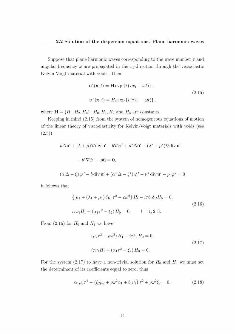
Suppose that plane harmonic waves corresponding to the wave number τ and
angular frequency ω are propagated in the x1-direction through the viscoelastic
Kelvin-Voigt material with voids. Then
u′ (x, t) = H exp i (τx1 − ωt) ,
ϕ ′ (x, t) = H0 exp i (τx1 − ωt) ,(2.15)
where H = (H1, H2, H3) ; H0, H1, H2 and H3 are constants.
Keeping in mind (2.15) from the system of homogeneous equations of motion
of the linear theory of viscoelasticity for Kelvin-Voigt materials with voids (see
(2.5))
µ∆u′ + (λ+ µ)∇div u′ + b∇ϕ ′ + µ∗∆u′ + (λ∗ + µ∗)∇div u′
+b∗∇ϕ ′ − ρu = 0,
(α∆− ξ)ϕ ′ − b div u′ + (α∗∆− ξ∗) ϕ ′ − ν∗ div u′ − ρ0ϕ′ = 0
it follows that
[µ1 + (λ1 + µ1) δ1l] τ2 − ρω2Hl − iτb1δ1lH0 = 0,
iτν1H1 + (α1τ2 − ξ2)H0 = 0, l = 1, 2, 3.
(2.16)
From (2.16) for H0 and H1 we have
(µ2τ2 − ρω2)H1 − iτb1H0 = 0,
iτν1H1 + (α1τ2 − ξ2)H0 = 0.
(2.17)
For the system (2.17) to have a non-trivial solution for H0 and H1 we must set
the determinant of its coefficients equal to zero, thus
α1µ2τ4 −
(ξ2µ2 + ρω2α1 + b1ν1
)τ 2 + ρω2ξ2 = 0. (2.18)
14
2.2 Solution of the dispersion equations. Plane harmonic waves
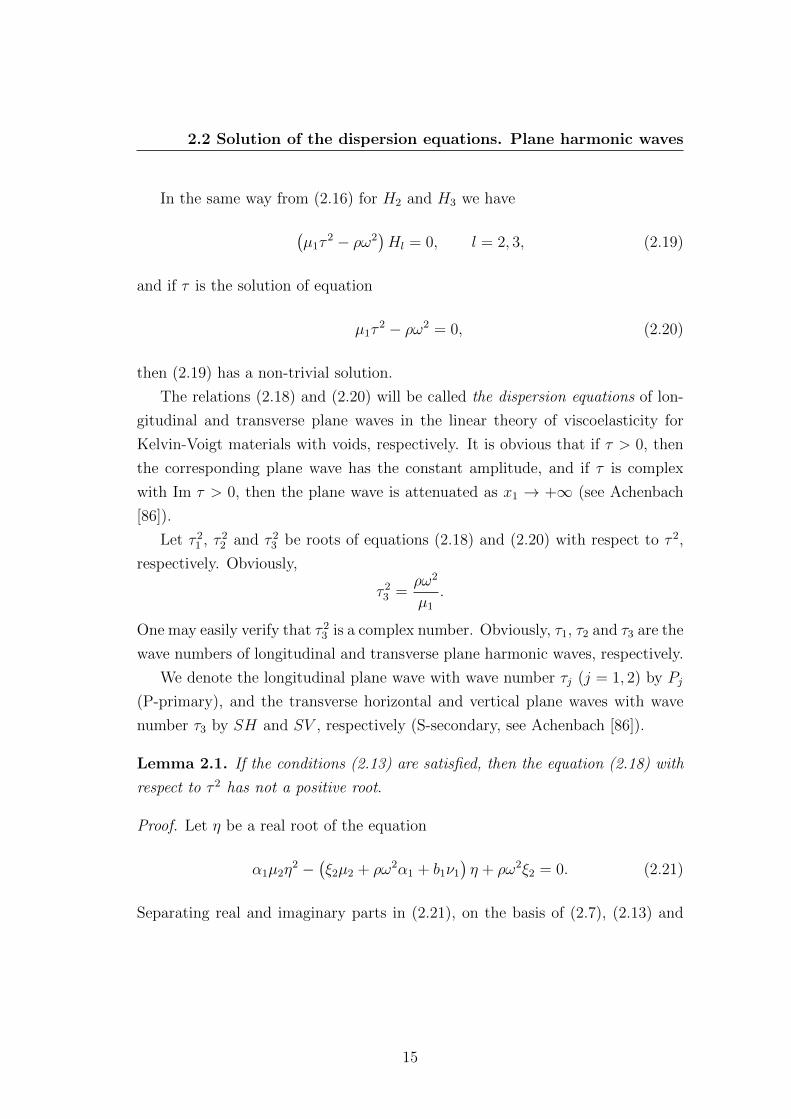
In the same way from (2.16) for H2 and H3 we have
(µ1τ
2 − ρω2)Hl = 0, l = 2, 3, (2.19)
and if τ is the solution of equation
µ1τ2 − ρω2 = 0, (2.20)
then (2.19) has a non-trivial solution.
The relations (2.18) and (2.20) will be called the dispersion equations of lon-
gitudinal and transverse plane waves in the linear theory of viscoelasticity for
Kelvin-Voigt materials with voids, respectively. It is obvious that if τ > 0, then
the corresponding plane wave has the constant amplitude, and if τ is complex
with Im τ > 0, then the plane wave is attenuated as x1 → +∞ (see Achenbach
[86]).
Let τ 21 , τ 2
2 and τ 23 be roots of equations (2.18) and (2.20) with respect to τ 2,
respectively. Obviously,
τ 23 =
ρω2
µ1
.
One may easily verify that τ 23 is a complex number. Obviously, τ1, τ2 and τ3 are the
wave numbers of longitudinal and transverse plane harmonic waves, respectively.
We denote the longitudinal plane wave with wave number τj (j = 1, 2) by Pj
(P-primary), and the transverse horizontal and vertical plane waves with wave
number τ3 by SH and SV , respectively (S-secondary, see Achenbach [86]).
Lemma 2.1. If the conditions (2.13) are satisfied, then the equation (2.18) with
respect to τ 2 has not a positive root.
Proof. Let η be a real root of the equation
α1µ2η2 −
(ξ2µ2 + ρω2α1 + b1ν1
)η + ρω2ξ2 = 0. (2.21)
Separating real and imaginary parts in (2.21), on the basis of (2.7), (2.13) and
15
2.2 Solution of the dispersion equations. Plane harmonic waves
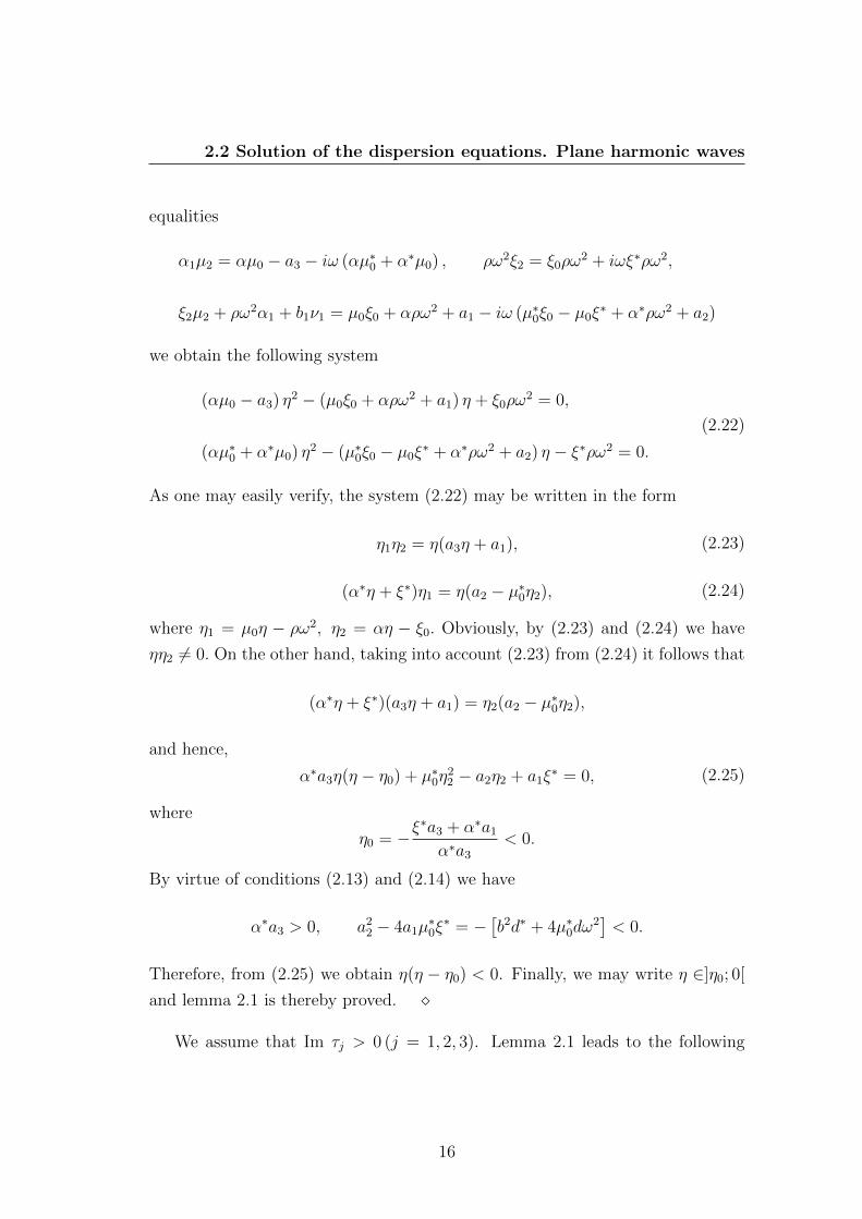
equalities
α1µ2 = αµ0 − a3 − iω (αµ∗0 + α∗µ0) , ρω2ξ2 = ξ0ρω2 + iωξ∗ρω2,
ξ2µ2 + ρω2α1 + b1ν1 = µ0ξ0 + αρω2 + a1 − iω (µ∗0ξ0 − µ0ξ∗ + α∗ρω2 + a2)
we obtain the following system
(αµ0 − a3) η2 − (µ0ξ0 + αρω2 + a1) η + ξ0ρω2 = 0,
(αµ∗0 + α∗µ0) η2 − (µ∗0ξ0 − µ0ξ∗ + α∗ρω2 + a2) η − ξ∗ρω2 = 0.
(2.22)
As one may easily verify, the system (2.22) may be written in the form
η1η2 = η(a3η + a1), (2.23)
(α∗η + ξ∗)η1 = η(a2 − µ∗0η2), (2.24)
where η1 = µ0η − ρω2, η2 = αη − ξ0. Obviously, by (2.23) and (2.24) we have
ηη2 6= 0. On the other hand, taking into account (2.23) from (2.24) it follows that
(α∗η + ξ∗)(a3η + a1) = η2(a2 − µ∗0η2),
and hence,
α∗a3η(η − η0) + µ∗0η22 − a2η2 + a1ξ
∗ = 0, (2.25)
where
η0 = −ξ∗a3 + α∗a1
α∗a3
< 0.
By virtue of conditions (2.13) and (2.14) we have
α∗a3 > 0, a22 − 4a1µ
∗0ξ∗ = −
[b2d∗ + 4µ∗0dω
2]< 0.
Therefore, from (2.25) we obtain η(η − η0) < 0. Finally, we may write η ∈]η0; 0[
and lemma 2.1 is thereby proved.
We assume that Im τj > 0 (j = 1, 2, 3). Lemma 2.1 leads to the following
16
2.3 Fundamental solution
result.
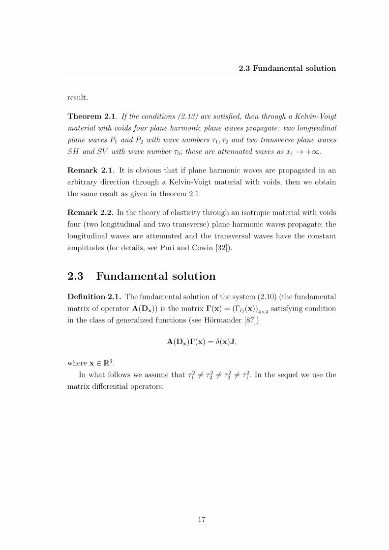
Theorem 2.1. If the conditions (2.13) are satisfied, then through a Kelvin-Voigt
material with voids four plane harmonic plane waves propagate: two longitudinal
plane waves P1 and P2 with wave numbers τ1, τ2 and two transverse plane waves
SH and SV with wave number τ3; these are attenuated waves as x1 → +∞.
Remark 2.1. It is obvious that if plane harmonic waves are propagated in an
arbitrary direction through a Kelvin-Voigt material with voids, then we obtain
the same result as given in theorem 2.1.
Remark 2.2. In the theory of elasticity through an isotropic material with voids
four (two longitudinal and two transverse) plane harmonic waves propagate; the
longitudinal waves are attenuated and the transversal waves have the constant
amplitudes (for details, see Puri and Cowin [32]).
2.3 Fundamental solution
Definition 2.1. The fundamental solution of the system (2.10) (the fundamental
matrix of operator A(Dx)) is the matrix Γ(x) = (Γlj(x))4×4 satisfying condition
in the class of generalized functions (see Hormander [87])
A(Dx)Γ(x) = δ(x)J,
where x ∈ R3.
In what follows we assume that τ 21 6= τ 2
2 6= τ 23 6= τ 2
1 . In the sequel we use the
matrix differential operators:
17
2.3 Fundamental solution
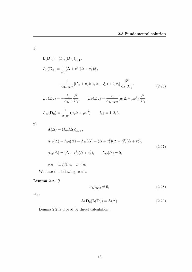
1)
L(Dx) = (Lpq(Dx))4×4 ,
Llj(Dx) =1
µ1
(∆ + τ 21 )(∆ + τ 2
2 )δlj
− 1
α1µ1µ2
[(λ1 + µ1)(α1∆ + ξ2) + b1ν1]∂2
∂xl∂xj,
Ll4(Dx) = − b1
α1µ1
∂
∂xl, L4l(Dx) =
ν1
α1µ1µ2
(µ1∆ + ρω2)∂
∂xl,
L44(Dx) =1
α1µ1
(µ2∆ + ρω2), l, j = 1, 2, 3.
(2.26)
2)
Λ(∆) = (Lpq(∆))4×4 ,
Λ11(∆) = Λ22(∆) = Λ33(∆) = (∆ + τ 21 )(∆ + τ 2
2 )(∆ + τ 23 ),
Λ44(∆) = (∆ + τ 21 )(∆ + τ 2
2 ), Λpq(∆) = 0,
p, q = 1, 2, 3, 4, p 6= q.
(2.27)
We have the following result.
Lemma 2.2. If
α1µ1µ2 6= 0, (2.28)
then
A(Dx)L(Dx) = Λ(∆). (2.29)
Lemma 2.2 is proved by direct calculation.
18
2.3 Fundamental solution
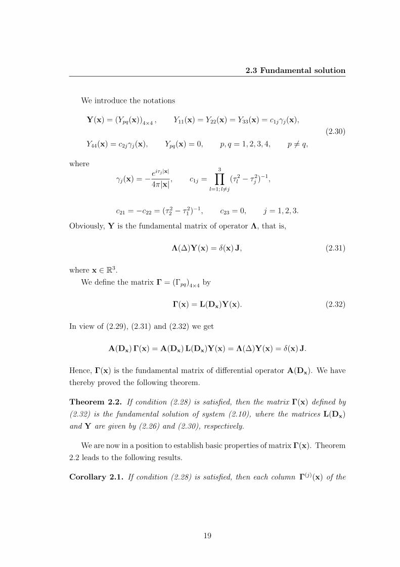
We introduce the notations
Y(x) = (Ypq(x))4×4 , Y11(x) = Y22(x) = Y33(x) = c1jγj(x),
Y44(x) = c2jγj(x), Ypq(x) = 0, p, q = 1, 2, 3, 4, p 6= q,
(2.30)
where
γj(x) = −eiτj |x|
4π|x|, c1j =
3∏l=1; l 6=j
(τ 2l − τ 2
j )−1,
c21 = −c22 = (τ 22 − τ 2
1 )−1, c23 = 0, j = 1, 2, 3.
Obviously, Y is the fundamental matrix of operator Λ, that is,
Λ(∆)Y(x) = δ(x) J, (2.31)
where x ∈ R3.
We define the matrix Γ = (Γpq)4×4 by
Γ(x) = L(Dx)Y(x). (2.32)
In view of (2.29), (2.31) and (2.32) we get
A(Dx) Γ(x) = A(Dx) L(Dx)Y(x) = Λ(∆)Y(x) = δ(x) J.
Hence, Γ(x) is the fundamental matrix of differential operator A(Dx). We have
thereby proved the following theorem.
Theorem 2.2. If condition (2.28) is satisfied, then the matrix Γ(x) defined by
(2.32) is the fundamental solution of system (2.10), where the matrices L(Dx)
and Y are given by (2.26) and (2.30), respectively.
We are now in a position to establish basic properties of matrix Γ(x). Theorem
2.2 leads to the following results.
Corollary 2.1. If condition (2.28) is satisfied, then each column Γ(j)(x) of the
19
2.3 Fundamental solution
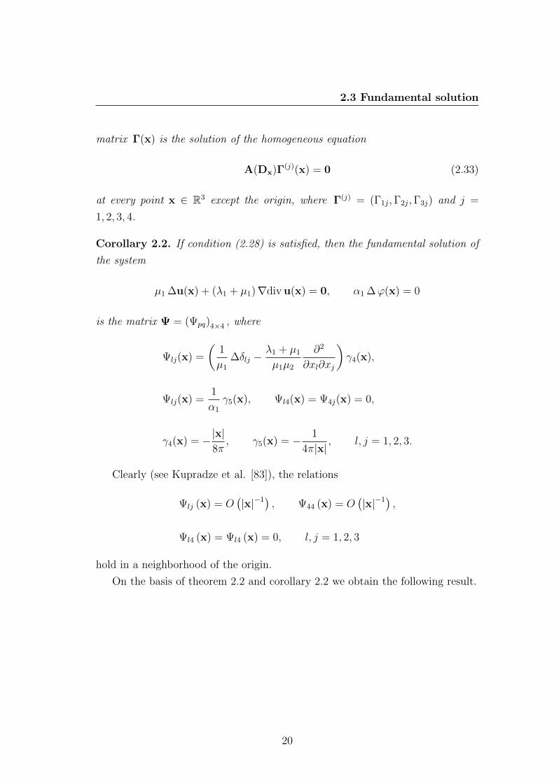
matrix Γ(x) is the solution of the homogeneous equation
A(Dx)Γ(j)(x) = 0 (2.33)
at every point x ∈ R3 except the origin, where Γ(j) = (Γ1j,Γ2j,Γ3j) and j =
1, 2, 3, 4.
Corollary 2.2. If condition (2.28) is satisfied, then the fundamental solution of
the system
µ1 ∆u(x) + (λ1 + µ1)∇div u(x) = 0, α1 ∆ϕ(x) = 0
is the matrix Ψ = (Ψpq)4×4 , where
Ψlj(x) =
(1
µ1
∆δlj −λ1 + µ1
µ1µ2
∂2
∂xl∂xj
)γ4(x),
Ψlj(x) =1
α1
γ5(x), Ψl4(x) = Ψ4j(x) = 0,
γ4(x) = −|x|8π, γ5(x) = − 1
4π|x|, l, j = 1, 2, 3.
Clearly (see Kupradze et al. [83]), the relations
Ψlj (x) = O(|x|−1) , Ψ44 (x) = O
(|x|−1) ,
Ψl4 (x) = Ψl4 (x) = 0, l, j = 1, 2, 3
hold in a neighborhood of the origin.
On the basis of theorem 2.2 and corollary 2.2 we obtain the following result.
20
2.3 Fundamental solution
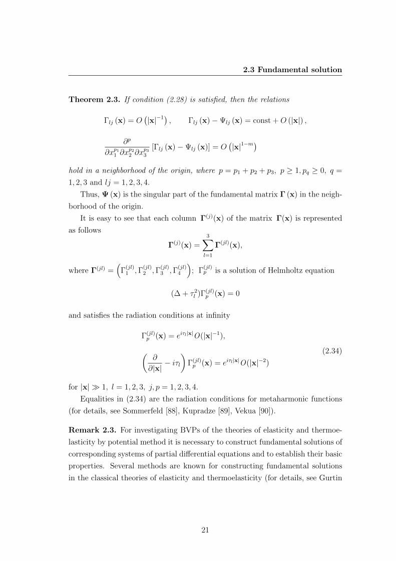
Theorem 2.3. If condition (2.28) is satisfied, then the relations
Γlj (x) = O(|x|−1) , Γlj (x)−Ψlj (x) = const +O (|x|) ,
∂p
∂xp11 ∂xp22 ∂x
p33
[Γlj (x)−Ψlj (x)] = O(|x|1−m
)hold in a neighborhood of the origin, where p = p1 + p2 + p3, p ≥ 1, pq ≥ 0, q =
1, 2, 3 and lj = 1, 2, 3, 4.
Thus, Ψ (x) is the singular part of the fundamental matrix Γ (x) in the neigh-
borhood of the origin.
It is easy to see that each column Γ(j)(x) of the matrix Γ(x) is represented
as follows
Γ(j)(x) =3∑l=1
Γ(jl)(x),
where Γ(jl) =(
Γ(jl)1 ,Γ
(jl)2 ,Γ
(jl)3 ,Γ
(jl)4
); Γ
(jl)p is a solution of Helmholtz equation
(∆ + τ 2l )Γ(jl)
p (x) = 0
and satisfies the radiation conditions at infinity
Γ(jl)p (x) = eiτl|x|O(|x|−1),
(∂
∂|x|− iτl
)Γ(jl)p (x) = eiτl|x|O(|x|−2)
(2.34)
for |x| 1, l = 1, 2, 3, j, p = 1, 2, 3, 4.
Equalities in (2.34) are the radiation conditions for metaharmonic functions
(for details, see Sommerfeld [88], Kupradze [89], Vekua [90]).
Remark 2.3. For investigating BVPs of the theories of elasticity and thermoe-
lasticity by potential method it is necessary to construct fundamental solutions of
corresponding systems of partial differential equations and to establish their basic
properties. Several methods are known for constructing fundamental solutions
in the classical theories of elasticity and thermoelasticity (for details, see Gurtin
21
2.4 Green’s formulas. Representations of general solutions
[91], Hetnarski and Ignaczak [92], Nowacki [93]). The explicit expressions of fun-
damental solutions in the theory of elasticity, thermoelasticity and micropolar
theory were obtained in different manner by Kupradze et al. [83], Sandru [94],
Dragos [95]. The basic properties of fundamental solutions of partial differential
equations are given in the book of Hormander [87].
2.4 Green’s formulas. Representations of gen-
eral solutions
In this section, first, we establish the Green’s formulas in the linear theory of
viscoelasticity for Kelvin-Voigt materials with voids, then we obtain the inte-
gral representation of regular vector (representation of Somigliana-type) and the
Galerkin-type solution of the system (2.6). Finally, we establish the representa-
tion of the general solution of the system of homogeneous equations (2.11) by
using metaharmonic functions.
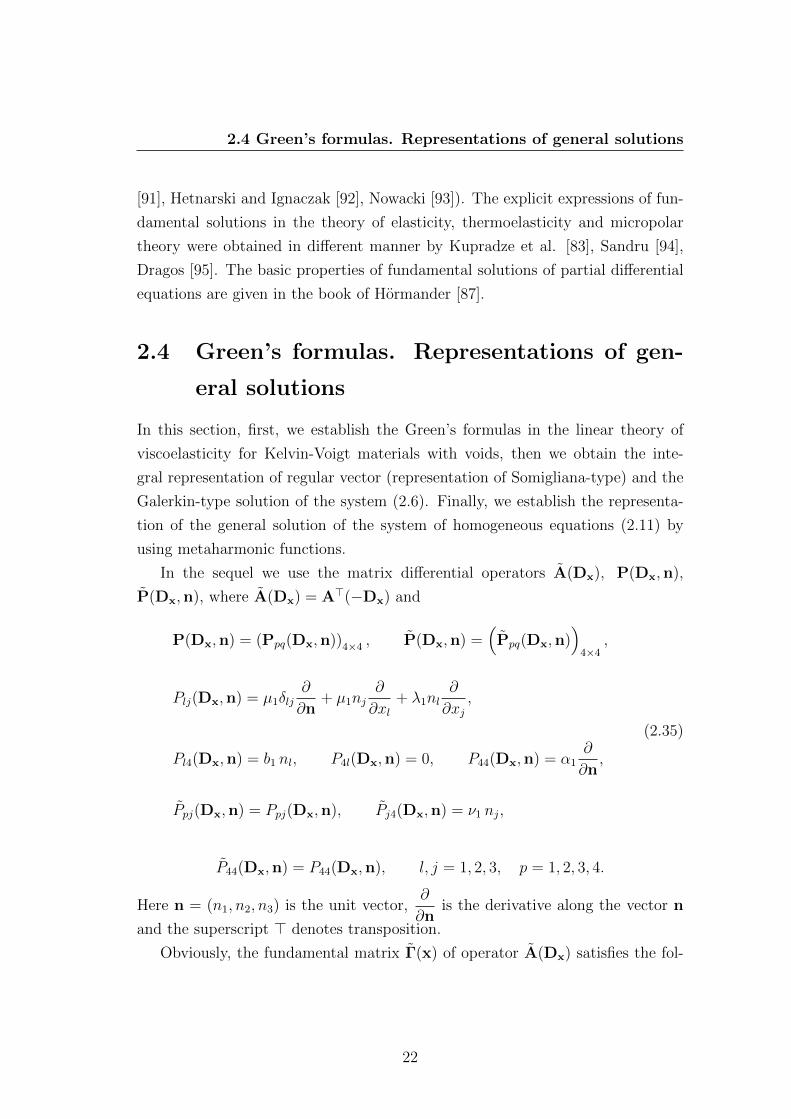
In the sequel we use the matrix differential operators A(Dx), P(Dx,n),
P(Dx,n), where A(Dx) = A>(−Dx) and
P(Dx,n) = (Ppq(Dx,n))4×4 , P(Dx,n) =(Ppq(Dx,n)
)4×4
,
Plj(Dx,n) = µ1δlj∂
∂n+ µ1nj
∂
∂xl+ λ1nl
∂
∂xj,
Pl4(Dx,n) = b1 nl, P4l(Dx,n) = 0, P44(Dx,n) = α1∂
∂n,
Ppj(Dx,n) = Ppj(Dx,n), Pj4(Dx,n) = ν1 nj,
(2.35)
P44(Dx,n) = P44(Dx,n), l, j = 1, 2, 3, p = 1, 2, 3, 4.
Here n = (n1, n2, n3) is the unit vector,∂
∂nis the derivative along the vector n
and the superscript > denotes transposition.
Obviously, the fundamental matrix Γ(x) of operator A(Dx) satisfies the fol-
22
2.4 Green’s formulas. Representations of general solutions
lowing condition
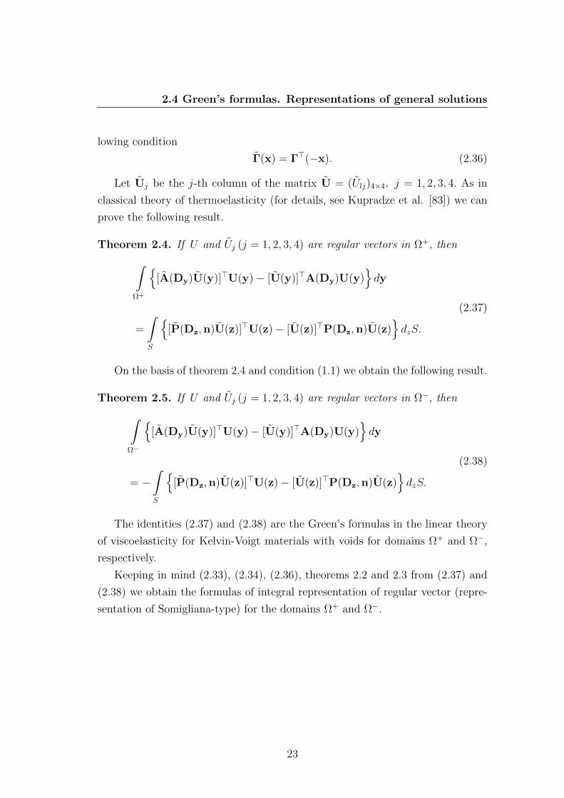
Γ(x) = Γ>(−x). (2.36)
Let Uj be the j-th column of the matrix U = (Ulj)4×4, j = 1, 2, 3, 4. As in
classical theory of thermoelasticity (for details, see Kupradze et al. [83]) we can
prove the following result.
Theorem 2.4. If U and Uj (j = 1, 2, 3, 4) are regular vectors in Ω+, then∫Ω+
[A(Dy)U(y)]>U(y)− [U(y)]>A(Dy)U(y)
dy
=
∫S
[P(Dz,n)U(z)]>U(z)− [U(z)]>P(Dz,n)U(z)
dzS.
(2.37)
On the basis of theorem 2.4 and condition (1.1) we obtain the following result.
Theorem 2.5. If U and Uj (j = 1, 2, 3, 4) are regular vectors in Ω−, then∫Ω−
[A(Dy)U(y)]>U(y)− [U(y)]>A(Dy)U(y)
dy
= −∫S
[P(Dz,n)U(z)]>U(z)− [U(z)]>P(Dz,n)U(z)
dzS.
(2.38)
The identities (2.37) and (2.38) are the Green’s formulas in the linear theory
of viscoelasticity for Kelvin-Voigt materials with voids for domains Ω+ and Ω−,
respectively.
Keeping in mind (2.33), (2.34), (2.36), theorems 2.2 and 2.3 from (2.37) and
(2.38) we obtain the formulas of integral representation of regular vector (repre-
sentation of Somigliana-type) for the domains Ω+ and Ω−.
23
2.4 Green’s formulas. Representations of general solutions
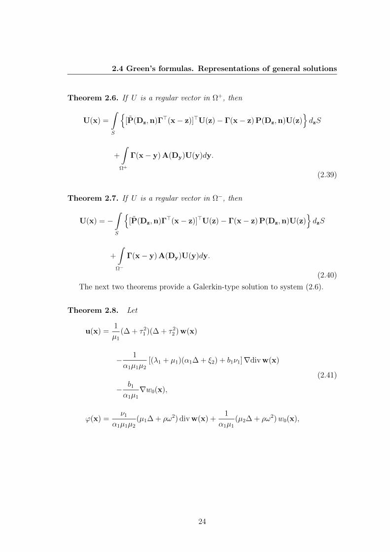
Theorem 2.6. If U is a regular vector in Ω+, then
U(x) =
∫S
[P(Dz,n)Γ>(x− z)]>U(z)− Γ(x− z) P(Dz,n)U(z)
dzS
+
∫Ω+
Γ(x− y) A(Dy)U(y)dy.
(2.39)
Theorem 2.7. If U is a regular vector in Ω−, then
U(x) = −∫S
[P(Dz,n)Γ>(x− z)]>U(z)− Γ(x− z) P(Dz,n)U(z)
dzS
+
∫Ω−
Γ(x− y) A(Dy)U(y)dy.
(2.40)
The next two theorems provide a Galerkin-type solution to system (2.6).
Theorem 2.8. Let
u(x) =1
µ1
(∆ + τ 21 )(∆ + τ 2
2 ) w(x)
− 1
α1µ1µ2
[(λ1 + µ1)(α1∆ + ξ2) + b1ν1]∇div w(x)
− b1
α1µ1
∇w0(x),
ϕ(x) =ν1
α1µ1µ2
(µ1∆ + ρω2) div w(x) +1
α1µ1
(µ2∆ + ρω2)w0(x),
(2.41)
24
2.4 Green’s formulas. Representations of general solutions
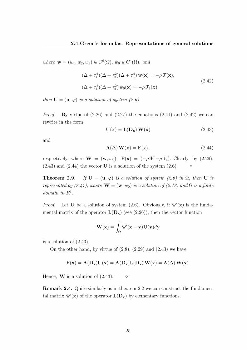
where w = (w1, w2, w3) ∈ C6(Ω), w0 ∈ C4(Ω), and
(∆ + τ 21 )(∆ + τ 2
2 )(∆ + τ 23 ) w(x) = −ρF(x),
(∆ + τ 21 )(∆ + τ 2
2 )w0(x) = −ρF4(x),
(2.42)
then U = (u, ϕ) is a solution of system (2.6).
Proof. By virtue of (2.26) and (2.27) the equations (2.41) and (2.42) we can
rewrite in the form
U(x) = L(Dx) W(x) (2.43)
and
Λ(∆) W(x) = F(x), (2.44)
respectively, where W = (w, w0), F(x) = (−ρF,−ρF4). Clearly, by (2.29),
(2.43) and (2.44) the vector U is a solution of the system (2.6).
Theorem 2.9. If U = (u, ϕ) is a solution of system (2.6) in Ω, then U is
represented by (2.41), where W = (w, w0) is a solution of (2.42) and Ω is a finite
domain in R3.
Proof. Let U be a solution of system (2.6). Obviously, if Ψ′(x) is the funda-
mental matrix of the operator L(Dx) (see (2.26)), then the vector function
W(x) =
∫Ω
Ψ′(x− y)U(y)dy
is a solution of (2.43).
On the other hand, by virtue of (2.8), (2.29) and (2.43) we have
F(x) = A(Dx)U(x) = A(Dx)L(Dx) W(x) = Λ(∆) W(x).
Hence, W is a solution of (2.43).
Remark 2.4. Quite similarly as in theorem 2.2 we can construct the fundamen-
tal matrix Ψ′(x) of the operator L(Dx) by elementary functions.
25
2.4 Green’s formulas. Representations of general solutions
Thus, on the basis of theorems 2.8 and 2.9 the completeness of Galerkin-type
solution of system (2.6) is proved.
Now we consider the system of homogeneous equations (2.10). We have the
following results.
Theorem 2.10. If metaharmonic function ϕj and metaharmonic vector func-
tion ψ = (ψ1, ψ2, ψ3) are solutions of equations
(∆ + τ 2j )ϕj(x) = 0, j = 1, 2 (2.45)
and
(∆ + τ 23 )ψ(x) = 0, divψ(x) = 0, (2.46)
respectively, then U = (u, ϕ) is a solution of the homogeneous equation (2.10),
whereu(x) = ∇ [c1 ϕ1(x) + c2 ϕ2(x)] +ψ(x),
ϕ(x) = ϕ1(x) + ϕ2(x)
(2.47)
for x ∈ Ω; Ω is an arbitrary domain in R3 and
cj =1
ρω2ν1
[(α1τ
2j − ξ2)µ2 − b1ν1
], j = 1, 2. (2.48)
Proof. Keeping in mind the relations (2.45)-(2.48) and
(−µ2τ2j + ρω2) cj + b1 = 0, j = 1, 2
26
2.4 Green’s formulas. Representations of general solutions
we obtain by direct calculation
µ1 ∆u + (λ1 + µ1)∇ div u + b1 gradϕ+ ρω2 u
= −µ1∇(c1τ21ϕ1 + c2τ
22ϕ2)− (λ1 + µ1)∇(c1τ
21ϕ1 + c2τ
22ϕ2)
+b1∇(ϕ1 + ϕ2) + ρω2∇(c1ϕ1 + c2ϕ2) + µ1∆ψ + ρω2ψ
= [(−µ2τ21 + ρω2) c1 + b1]∇ϕ1 + [(−µ2τ
22 + ρω2) c2 + b1]∇ϕ2 = 0.
Quite similarly, by virtue of (2.47) and
ν1τ2j cj − α1τ
2j + ξ2 = 0, j = 1, 2
we have
(α1 ∆ + ξ2)ϕ− ν1 div u = −(α1τ21 − ξ2)ϕ1 − (α1τ
22 − ξ2)ϕ2 + ν1(c1τ
21ϕ1 + c2τ
22ϕ2)
= (ν1τ21 c1 − α1τ
21 + ξ2)ϕ1 + (ν1τ
22 c2 − α1τ
21 + ξ2)ϕ2 = 0.
Theorem 2.11. If U = (u, ϕ) is a solution of the homogeneous equation (2.10)
in Ω, then U is represented by (2.47), where ϕj and ψ = (ψ1, ψ2, ψ3) are so-
lutions of (2.45) and (2.46), respectively; Ω is an arbitrary domain in R3 and
cj (j = 1, 2) is given by (2.48).
Proof. Applying the operator div to the first equation of (2.10) from system
(2.10) we have
(µ2 ∆ + ρω2) div u + b1 ∆ϕ = 0,
(α1 ∆ + ξ2)ϕ− ν1 div u = 0.
(2.49)
Clearly, we obtain from (2.49)
(∆ + τ 21 )(∆ + τ 2
2 )ϕ = 0. (2.50)
27
2.4 Green’s formulas. Representations of general solutions
Now applying the operator curl to the first equation of (2.10) it follows that
(∆ + τ 23 ) curl u = 0. (2.51)
We introduce the notation
ϕ1 =1
τ 22 − τ 2
1
(∆ + τ 22 )ϕ, ϕ2 =
1
τ 21 − τ 2
2
(∆ + τ 21 )ϕ,
ψ =µ1
ρω2curl curl u.
(2.52)
Taking into account (2.50) - (2.52), the function ϕj and vector function ψ are
the solutions of (2.45) and (2.46), respectively, and the function ϕ is represented
by (2.47).
Now we prove the first relation of (2.47). Obviously, on the basis of (2.45) the
second equation of (2.49) we can rewrite in the form
div u = c3ϕ1 + c4ϕ2, (2.53)
where
cj =1
ν1
(ξ2 − α1τ2j−2), j = 3, 4.
Keeping in mind (2.52), (2.53) and identity
∆u = ∇div u− curl curl u
from (2.49) we obtain
u = − 1
ρω2∇[µ2 div u + b1 ϕ] +ψ
= − 1
ρω2∇[(µ2c3 + b1)ϕ1 + (µ2c4 + b1)ϕ2] +ψ.
(2.54)
Finally, from (2.54) we get the first relation of (2.47).
Hence, on the basis of theorems 2.10 and 2.11 the completeness of solution of
28
2.4 Green’s formulas. Representations of general solutions
the homogeneous equation (2.10) is proved.
Remark 2.5. Contemporary treatment of the various BVPs of the theories of
elasticity and thermoelasticity usually begins with the representation of a solution
of field equations in terms of elementary (harmonic, biharmonic, metaharmonic
and etc.) functions. In the classical theories of elasticity and thermoelastic-
ity the Boussinesq-Somigliana-Galerkin, Boussinesq-Papkovitch-Neuber, Green-
Lame, Naghdi-Hsu and Cauchy-Kovalevski-Somigliana solutions are well known
(for details, see Gurtin [91], Hetnarski and Ignaczak [92]). A review of the history
of these solutions is given in Wang et al. [96]. The Galerkin type solution (see
Galerkin [97]) of equations of classical elastokinetics was obtained by Iacovache
[99]. In the linear theory of elasticity for materials with voids, the Boussinesq-
Papkovitch-Neuber, Green-Lame and Cauchy-Kovalevski-Somigliana type solu-
tions were obtained by Chandrasekharaiah [99, 100]. The representation theorem
of Galerkin type in the theory of thermoelasticity for materials with voids was
proved by Ciarletta [43].
29
Chapter 3
Boundary value problems in the
theory of viscoelasticity for
materials with voids
3.1 Basic boundary value problems
The basic internal and external BVPs of steady vibration in the theory of vis-
coelasticity for Kelvin-Voigt materials with voids are formulated as follows.
Find a regular (classical) solution to system (2.9) for x ∈ Ω+ satisfying the
boundary condition
limΩ+3x→z∈S
U(x) ≡ U(z)+ = f(z) (3.1)
in the Problem (I)+F,f , and
P(Dz,n(z))U(z)+ = f(z) (3.2)
in the Problem (II)+F,f , where the matrix differential operator P(Dz,n(z)) is
defined by (2.35), F and f are the known four-component vector functions.
Find a regular (classical) solution to system (2.9) for x ∈ Ω− satisfying the
30
3.2 Uniqueness theorems
boundary condition
limΩ−3x→z∈S
U(x) ≡ U(z)− = f(z) (3.3)
in the Problem (I)−F,f , and
P(Dz,n(z))U(z)− = f(z) (3.4)
in the Problem (II)−F,f . Here F and f are the known four-component vector
functions, supp F is a finite domain in Ω−, and n(z) is the external (with respect
to Ω+) unit normal vector to S at z.
In the Sections 3.2 and 3.4 the uniqueness and existence theorems for classical
solutions of the BVPs (K)+F,f and (K)−F,f are proved by using the potential method
and the theory of singular integral equations, respectively, where K = I, II.
3.2 Uniqueness theorems
In the sequel we use the matrix differential operators
B(Dx) = (Blj(Dx))3×3, T(Dx,n) = (Tlj(Dx,n))3×3,
where
Blj(Dx) = µ1∆δlj + (λ1 + µ1)∂2
∂xl∂xj,
Tlj(Dx,n) = µ1δlj∂
∂n+ µ1nj
∂
∂xl+ λ1nl
∂
∂xj, l, j = 1, 2, 3.
Obviously, T(Dx,n) is the stress operator in the classical theory of elasticity (see
Kupradze et al. [83]).
31
3.2 Uniqueness theorems
Theorem 3.1. If conditions
µ∗ > 0, 3λ∗ + 2µ∗ > 0, α∗ > 0,
(3λ∗ + 2µ∗)ξ∗ >3
4(b∗ + ν∗)2
(3.5)
are satisfied, then the internal BVP (K)+F,f admits at most one regular solution,
where K = I, II.
Proof. Suppose that there are two regular solutions of problem (K)+F,f . Then their
difference U corresponds to zero data (F = f = 0), i.e. U is a regular solution of
problem (K)+0,0.
On account of (2.10) from Green’s formulas of the classical theory of elasticity
(see Kupradze et al. [83])∫Ω+
[B(Dx) u · u +W (u, λ1, µ1)] dx =
∫S
Tu · u dzS,
∫Ω+
[∆ϕϕ+ |∇ϕ|2
]dx =
∫S
∂ϕ
∂nϕ dzS
and identity ∫Ω+
(∇ϕ · u + ϕ divu) dx =
∫S
ϕn · u dzS
it follows that∫Ω+
[W (u, λ1, µ1)− ρω2 |u|2 + b1 ϕ div u
]dx =
∫S
(Tu + b1 ϕn) · u dzS,
∫Ω+
[α1 |∇ϕ|2 − ξ2 |ϕ|2 + ν1 div u ϕ
]dx = α1
∫S
∂ϕ
∂nϕ dzS,
(3.6)
32
3.2 Uniqueness theorems
where
W (u, λ1, µ1) =1
3(3λ1 + 2µ1) |div u|2
+µ1
[1
2
3∑l,j=1; l 6=j
∣∣∣∣∂uj∂xl+∂ul∂xj
∣∣∣∣2 +1
3
3∑l,j=1
∣∣∣∣∂ul∂xl− ∂uj∂xj
∣∣∣∣2].
(3.7)
Clearly, W (u, λ1, µ1) = W (u, λ, µ)− iωW (u, λ∗, µ∗). In view of (3.6) we get∫Ω+
[W (u, λ1, µ1)− ρω2 |u|2 + α1 |∇ϕ|2 − ξ2 |ϕ|2 + (b1 ϕ div u + ν1 div u ϕ)
]dx
=
∫S
[(Tu + b1 ϕn) · u + α1
∂ϕ
∂nϕ
]dzS,
and on the basis of homogeneous boundary condition and the identity
Im (b1 ϕ div u + ν1 div u ϕ) = −ω(b∗ + ν∗) Re(ϕ div u)
we obtain∫Ω+
[W (u, λ∗, µ∗)− (b∗ + ν∗) Re(ϕ div u) + ξ∗ |ϕ|2 + α∗ |∇ϕ|2
]dx = 0. (3.8)
Obviously, with the help of (3.5) it follows that
1
3(3λ∗ + 2µ∗)|div u|2 − (b∗ + ν∗) Re(ϕ div u) + ξ∗ |ϕ|2 ≥ 0
and from (3.8) we have
W (u, λ∗, µ∗)− (b∗ + ν∗) Re(ϕ div u) + ξ∗ |ϕ|2 + α∗ |gradϕ|2 = 0.
It is easy to verify that on the basis of (3.5) the last equation leads to the following
33
3.2 Uniqueness theorems
relations
ϕ(x) = 0, div u(x) = 0,∂uj∂xl
+∂ul∂xj
= 0,
∂ul∂xl− ∂uj∂xj
= 0, l, j = 1, 2, 3
(3.9)
for x ∈ Ω+. In view of (3.9) we get W (u, λ, µ) = 0 and W (u, λ∗, µ∗) = 0. Hence,
W (u, λ1, µ1) = 0. Finally, from the first equation of (3.6) we obtain u(x) = 0.
Thus, U(x) = 0 for x ∈ Ω+.
Lemma 3.1. If U = (u, ϕ) ∈ C2(Ω) is a solution of the system (2.10) for x ∈ Ω,
then
u(x) =3∑j=1
u(j)(x), ϕ(x) =2∑l=1
ϕ(l)(x), (3.10)
where Ω is an arbitrary domain in R3, u(j) and ϕ(l) satisfy the following equations
(∆ + τ 2j )u(j)(x) = 0, (∆ + τ 2
l )ϕ(l)(x) = 0,
l = 1, 2, j = 1, 2, 3.
(3.11)
Proof. Applying the operator div to the first equation of (2.10) we get
(µ2∆ + ρω2) div u + b1 ∆ϕ = 0,
(α1 ∆ + ξ2)ϕ− ν1 div u = 0.
(3.12)
Clearly, from system (3.12) we have
(∆ + τ 21 ) (∆ + τ 2
2 ) div u = 0,
(∆ + τ 21 ) (∆ + τ 2
2 )ϕ = 0.
(3.13)
Now, applying the operator (∆ + τ 21 ) (∆ + τ 2
2 ) to the first equation of (2.10)
and using (3.13) we obtain
(∆ + τ 21 ) (∆ + τ 2
2 ) (∆ + τ 23 ) u = 0. (3.14)
34
3.2 Uniqueness theorems
We introduce the notation
u(j) =3∏
p=1;p6=j
(τ 2p − τ 2
j )−1(∆ + τ 2p ) u, j = 1, 2, 3,
ϕ(l) =2∏
p=1;p 6=l
(τ 2p − τ 2
l )−1(∆ + τ 2p )ϕ, l = 1, 2.
(3.15)
By virtue of (3.13) and (3.14) the relations (3.10) and (3.11) can be easily
obtained from (3.15). Now let us establish the uniqueness of a regular solution of external BVPs.
Theorem 3.2. If conditions (3.5) are satisfied, then the external BVP (K)−F,fadmits at most one regular solution, where K = I, II.
Proof. Suppose that there are two regular solutions of problem (K)−F,f . Then
their difference U = (U1, U2, U3, U4) corresponds to zero data (F = f = 0), i.e. U
is a regular solution of the problem (K)−0,0.
Let Ωr be a sphere of sufficiently large radius r so that Ω+ ⊂ Ωr . By virtue
of homogeneous boundary condition (f = 0), the formula (2.36) for the domain
Ω−r = Ω− ∩ Ωr can be rewritten as∫Ω−r
[W (u, λ1, µ1)− ρω2|u|2 + α1|∇ϕ|2 − ξ2|ϕ|2 + (b1 ϕ div u + ν1 div u ϕ)
]dx
=
∫Sr
[(Tu + b1 ϕn) · u + α1
∂ϕ
∂nϕ
]dzS,
(3.16)
where Sr is the boundary of the sphere Ωr. From (3.16) we have
N = limr→∞
∫Sr
[(Tu + b1 ϕn) · u + α1
∂ϕ
∂nϕ
]dzS, (3.17)
35
3.3 Basic properties of elastopotentials
where
N =
∫Ω−
[W (u, λ∗, µ∗)− (b∗ + ν∗) Re(ϕ div u) + ξ∗ |ϕ|2 + α∗ |∇ϕ|2
]dx. (3.18)
Obviously, by condition (3.5) it follows from (3.18) that N ≥ 0.
On the other hand, keeping in mind the conditions (1.1), (2.34) and (3.10)
from (2.40) we obtain
Uj(x) = e−τ0|x|O(|x|−1),
Uj,l(x) = e−τ0|x|O(|x|−1) for |x| 1,
(3.19)
where τ0 = min Im τ1, Im τ2, Im τ3 > 0, l = 1, 2, 3, j = 1, 2, 3, 4. On account of
(3.19) from (3.17) it follows that N = 0. Hence, from (3.18) we get∫Ω−
[W (u, λ∗, µ∗)− (b∗ + ν∗) Re(ϕ div u) + ξ∗ |ϕ|2 + α∗ |gradϕ|2
]dx = 0. (3.20)
Quite similarly as in theorem 3.1 on the basis of (3.5) from (3.20) we obtain
U(x) = 0 for x ∈ Ω−.
Remark 3.1. The uniqueness theorems in the linear theory of elasticity for
materials with voids are proved by Chandrasekharaiah [34]. Basic results as well
as an extensive review on uniqueness theorems in the classical theory of elasticity
can be found in the books by Knops and Payne [101], Kupradze et al. [83].
3.3 Basic properties of elastopotentials
On the basis of Somigliana-type integral representation of regular vector (see,
(2.39)) we introduce the following notations
Z(1)(x,g) =
∫S
Γ(x− y)g(y)dyS,
36
3.3 Basic properties of elastopotentials
Z(2)(x,g) =
∫S
[P(Dy,n(y))Γ>(x− y)]>g(y)dyS,
Z(3)(x,φ,Ω±) =
∫Ω±
Γ(x− y)φ(y)dy,
where g and φ are four-component vectors.
As in classical theory of elasticity (see, e.g. Kupradze et al. [83]), the vector
functions Z(1)(x,g), Z(2)(x,g) and Z(3)(x,φ,Ω±) are called single-layer, double-
layer and volume potentials in the linear theory of viscoelasticity for Kelvin-Voigt
materials with voids, respectively.
Obviously, on the basis of (2.39) and (2.40), the regular vector in Ω+ and Ω−
is represented by sum of the elastopotentials as follows
U(x) = Z(2)(x, U+
)− Z(1)
(x, PU+
)+ Z(3)
(x,AU,Ω+
)for x ∈ Ω+
and
U(x) = −Z(2)(x, U−
)+ Z(1)
(x, PU−
)+ Z(3)
(x,AU,Ω−
)for x ∈ Ω−,
respectively.
First we establish the basic properties of elastopotentials.
Theorem 3.3. If S ∈ Cj+1,p, g ∈ Cj,p ′(S), 0 < p ′ < p ≤ 1, and j is a non-
negative integer, then:
a)
Z(1)(·,g) ∈ C0,p ′(R3) ∩ Cj+1,p ′(Ω±) ∩ C∞(Ω±),
b)
A(Dx) Z(1)(x,g) = 0, x ∈ Ω±,
c)
P(Dz,n(z)) Z(1)(z,g)± = ∓ 1
2g(z) + P(Dz,n(z)) Z(1)(z,g), z ∈ S, (3.21)
37
3.3 Basic properties of elastopotentials
d)
P(Dz,n(z)) Z(1)(z,g)
is a singular integral for z ∈ S.
Theorem 3.4. If S ∈ Cj+1,p, g ∈ Cj,p ′(S), 0 < p ′ < p ≤ 1, then:
a)
Z(2)(·,g) ∈ Cj,p ′(Ω±) ∩ C∞(Ω±),
b)
A(Dx) Z(2)(x,g) = 0, x ∈ Ω±,
c)
Z(2)(z,g)± = ± 1
2g(z) + Z(2)(z,g), z ∈ S (3.22)
for the non-negative integer j,
d)
Z(2)(z,g)
is a singular integral for z ∈ S,e)
P(Dz,n(z)) Z(2)(z,g)+ = P(Dz,n(z)) Z(2)(z,g)−,
for the natural number j and z ∈ S.
Theorem 3.5. If S ∈ C1,p, φ ∈ C0,p ′(Ω+), 0 < p ′ < p ≤ 1, then:
a)
Z(3)(·,φ,Ω+) ∈ C1,p′(R3) ∩ C2(Ω+) ∩ C2,p′(Ω+0 ),
b)
A(Dx) Z(3)(x,φ,Ω+) = φ(x), x ∈ Ω+,
where Ω+0 is a domain in R3 and Ω+
0 ⊂ Ω+.
Theorem 3.6. If S ∈ C1,p, suppφ = Ω ⊂ Ω−, φ ∈ C0,p ′(Ω−), 0 < p ′ < p ≤ 1,
then:
a)
Z(3)(·,φ,Ω−) ∈ C1,p′(R3) ∩ C2(Ω−) ∩ C2,p′(Ω−0 ),
38
3.3 Basic properties of elastopotentials
b)
A(Dx) Z(3)(x,φ,Ω−) = φ(x), x ∈ Ω−,
where Ω is a finite domain in R3 and Ω−0 ⊂ Ω−.
Theorems 3.3 to 3.6 can be proved similarly to the corresponding theorems in
the classical theory of thermoelasticity (for details, see Kupradze et al. [83]).
We introduce the notations
K(1)g(z) ≡ 1
2g(z) + Z(2)(z,g),
K(2)g(z) ≡ −1
2g(z) + P(Dz,n(z))Z(1)(z,g),
K(3)g(z) ≡ −1
2g(z) + Z(2)(z,g),
K(4)g(z) ≡ 1
2g(z) + P(Dz,n(z))Z(1)(z,g),
Kζg(z) ≡ −1
2g(z) + ζ Z(2)(z,g) for z ∈ S,
(3.23)
where ζ is a complex parameter. On the basis of theorems 3.3 and 3.4, K(j) (j =
1, 2, 3, 4) and Kζ are singular integral operators (for the definition a singular
integral operator see, e.g. Mikhlin [81]).
In the sequel we need the following Lemmas.
Lemma 3.2. If conditions (3.5) are satisfied, then the singular integral oper-
ator K(j)(j = 1, 2, 3, 4) is of the normal type.
Proof: Let σ(j) = (σ(j)lm)4×4 be the symbol of the singular integral operator
K(j) (j = 1, 2, 3.4) (see, e.g. Mikhlin [81]). Taking into account (3.23) we find
(for details, see, Kupradze et al. [83], Ch. IV)
det σ(j) =
(−1
2
)4 [1− µ2
1
(λ1 + 2µ1)2
]=
(λ1 + µ1)(λ1 + 3µ1)
16(λ1 + 2µ1)2. (3.24)
39
3.3 Basic properties of elastopotentials
Keeping in mind the relations (3.5) from (3.24) we have
det σ(j) 6= 0. (3.25)
Hence, the operator K(j) is of the normal type, where j = 1, 2, 3, 4.
Lemma 3.3. If L is a continuous curve on the complex plane connecting the
origin with the point ζ0 and Kζ is a normal type operator for any ζ ∈ L, then the
index of the operator Kζ0 vanishes, i.e.
ind Kζ0 = 0.
Lemma 3.3 for the singular integral operators is proved in Kupradze et al.
[83], Ch. IV.
Lemma 3.4. If conditions (3.5) are satisfied, then the Fredholm’s theorems
are valid for the singular integral operator K(j) (K(j) is Fredholmian), where
j = 1, 2, 3, 4.
Proof: Let σζ and indKζ be the symbol and the index of the operator Kζ ,
respectively. It may be easily shown that
det σζ =(λ1 + 2µ1)2 − µ2
1ζ2
16(λ1 + 2µ1)2
and detσζ vanishes only at two points ζ1 and ζ2 of the complex plane. By virtue
of (3.25) and detσ1 = detσ(1) we get ζj 6= 1 for j = 1, 2. By Lemma 3.3 we
obtain
indK(1) = indK1 = 0.
Equation indK(2) = 0 is proved in a quite similar manner. Obviously, the
operators K(3) and K(4) are the adjoint operators for K(2) and K(1), respectively.
Evidently,
indK(3) = −indK(2) = 0, indK(4) = −indK(1) = 0.
40
3.4 Existence theorems
Thus, the singular integral operator K(j) (j = 1, 2, 3, 4) is of the normal type
with an index equal to zero. Consequently, the Fredholm’s theorems are valid for
K(j) (for details, see, e.g. Mikhlin [81]).
Remark 3.2. The definitions of a normal type singular integral operator, the
symbol and the index of operator are given in Mikhlin [81] and Kupradze et al.
[83].
3.4 Existence theorems
Obviously, by theorems 3.5 and 3.6 the volume potential Z(3)(x,F,Ω±) is a regular
solution of (2.9), where F ∈ C0,p ′(Ω±), 0 < p ′ ≤ 1; supp F is a finite domain in
Ω−. Therefore, further we will consider problem (K)±0,f for K = I, II. In addition,
we assume that the conditions (3.5) are satisfied.
Now we prove the existence theorems of a regular (classical) solution of prob-
lems (K)−0,f and (K)−0,f for K = I, II.
Problem (I)+0,f . We seek a regular solution to problem (I)+
0,f in the form
U(x) = Z(2)(x,g) for x ∈ Ω+, (3.26)
where g is the required four-component vector function.
By theorem 3.4 the vector function U is a solution of (2.11) for x ∈ Ω+.
Keeping in mind the boundary condition (3.1) and using (3.22), from (3.26) we
obtain, for determining the unknown vector g, a singular integral equation
K(1)g(z) = f(z) for z ∈ S. (3.27)
By lemma 3.4 the Fredholm’s theorems are valid for operator K(1). We prove that
(3.27) is always solvable for an arbitrary vector f . Let us consider the associate
homogeneous equation
K(4)h0(z) = 0 for z ∈ S, (3.28)
41
3.4 Existence theorems
where h0 is the required four-component vector function. Now we prove that
(3.28) has only the trivial solution.
Indeed, let h0 be a solution of the homogeneous equation (3.28). On the basis
of theorem 3.3 and (3.28) the vector function V(x) = Z(1)(x,h0) is a regular
solution of problem (II)−0,0. Using theorem 3.2, the problem (II)−0,0 has only the
trivial solution, that is
V(x) = 0 for x ∈ Ω−. (3.29)
On other hand, by theorem 3.3 and (3.29) we get
V(z)+ = V(z)− = 0 for z ∈ S,
i.e., the vector V(x) is a regular solution of problem (I)+0,0. Using theorem 3.1,
the problem (I)+0,0 has only the trivial solution, that is
V(x) = 0 for x ∈ Ω+. (3.30)
By virtue of (3.29), (3.30) and identity (3.21) we obtain
h0(z) = P(Dz,n)V(z)− − P(Dz,n)V(z)+ = 0 for z ∈ S.
Thus, the homogeneous equation (3.28) has only the trivial solution and therefore
(3.27) is always solvable for an arbitrary vector f .
We have thereby proved
Theorem 3.7. If S ∈ C2,p, f ∈ C1,p ′(S), 0 < p ′ < p ≤ 1, then a regular
solution of problem (I)+0,f exists, is unique and is represented by double-layer
potential (3.26), where g is a solution of the singular integral equation (3.27)
which is always solvable for an arbitrary vector f .
Problem (II)−0,f . We seek a regular solution to problem (II)−0,f in the form
U(x) = Z(1)(x,h) for x ∈ Ω−, (3.31)
42
3.4 Existence theorems
where h is the required four-component vector function.
Obviously, by theorem 3.3 the vector function U is a solution of (2.11) for x ∈Ω−. Keeping in mind the boundary condition (3.4) and using (3.21), from (3.31)
we obtain, for determining the unknown vector h, a singular integral equation
K(4)h(z) = f(z) for z ∈ S. (3.32)
It has been proved above that the corresponding homogeneous equation (3.28)
has only the trivial solution. Hence, it follows that (3.32) is always solvable.
We have thereby proved
Theorem 3.8. If S ∈ C2,p, f ∈ C0,p ′(S), 0 < p ′ < p ≤ 1, then a regular
solution of problem (II)−0,f exists, is unique and is represented by single-layer
potential (3.31), where h is a solution of the singular integral equation (3.32)
which is always solvable for an arbitrary vector f .
Problem (II)+0,f . We seek a regular solution to problem (II)+
0,f in the form
U(x) = Z(1)(x,g) for x ∈ Ω+, (3.33)
where g is the required four-component vector function.
Obviously, by theorem 3.3 the vector function U is a solution of (2.11) for x ∈Ω+. Keeping in mind the boundary condition (3.2) and using (3.21), from (3.33)
we obtain, for determining the unknown vector g, a singular integral equation
K(2)g(z) = f(z) for z ∈ S. (3.34)
By lemma 3.4 the Fredholm’s theorems are valid for operator K(2). We prove
that (3.34) is always solvable for an arbitrary vector f . Let us consider the
corresponding homogeneous equation
K(2)g0(z) = 0 for z ∈ S, (3.35)
where g0 is the required four-component vector function. Now we prove that
(3.35) has only the trivial solution.
43
3.4 Existence theorems
Indeed, let g0 be a solution of the homogeneous equation (3.35). On the basis
of theorem 3.3 and (3.35) the vector V(x) = Z(1)(x,g0) is a regular solution
of problem (II)+0,0. Using theorem 3.1, the problem (II)+
0,0 has only the trivial
solution, that is
V(x) = 0 for x ∈ Ω+. (3.36)
On other hand, by theorem 3.3 and (3.36) we get V(z)− = 0 for z ∈ S, i.e.,
the vector V(x) is a regular solution of problem (I)−0,0. On the basis of theorem
3.2, the problem (I)−0,0 has only the trivial solution, that is
V(x) = 0 for x ∈ Ω−. (3.37)
By virtue of (3.36), (3.37) and identity (3.21) we obtain
g0(z) = P(Dz,n)V(z)− − P(Dz,n)V(z)+ = 0 for z ∈ S.
Thus, the homogeneous equation (3.35) has only a trivial solution and therefore
(3.34) is always solvable for an arbitrary vector f .
We have thereby proved
Theorem 3.9. If S ∈ C2,p, f ∈ C0,p ′(S), 0 < p ′ < p ≤ 1, then a regular
solution of problem (II)+0,f exists, is unique and is represented by single-layer
potential (3.33), where g is a solution of the singular integral equation (3.34)
which is always solvable for an arbitrary vector f .
Problem (I)−0,f . We seek a regular solution to problem (I)−0,f in the form
U(x) = Z(2)(x,h) for x ∈ Ω−, (3.38)
where h is the required four-component vector function.
Obviously, by theorem 3.4 the vector function U is a solution of (2.11) for x ∈Ω−. Keeping in mind the boundary condition (3.3) and using (3.22), from (3.38)
we obtain, for determining the unknown vector h, a singular integral equation
K(3)h(z) = f(z) for z ∈ S. (3.39)
44
3.4 Existence theorems
It has been proved above that the corresponding homogeneous equation (3.35)
has only the trivial solution. Hence, it follows that (3.39) is always solvable.
We have thereby proved
Theorem 3.10. If S ∈ C2,p, f ∈ C1,p ′(S), 0 < p ′ < p ≤ 1, then a regular
solution of problem (I)−0,f exists, is unique and is represented by double-layer
potential (3.38), where h is a solution of the singular integral equation (3.39)
which is always solvable for an arbitrary vector f .
Remark 3.3. In Pompei and Scalia [102], the BVPs of steady vibrations of
the linear theory of elasticity for materials with voids are investigated. The
potentials of single layer and double layer are used to reduce the BVPs to singular
integral equations for which Fredholm’s basic theorems are valid. Existence and
uniqueness results for external problems are established.
45

Chapter 4
Solutions of equations in the
theory of thermoviscoelasticity
for materials with voids
4.1 Basic Equations
The complete system of field equations in the linear theory of thermoviscoelastic-
ity for Kelvin-Voigt material with voids consists of the following equations (Iesan
[62]):
1) The equations of motion (2.1) and (2.2);
2) The constitutive equations
t′lj = 2µ e′lj + λ e′rrδlj + bϕ′δlj + 2µ∗ e′lj + λ∗ e′rrδlj + b∗ϕ′ δlj − β θ′ δlj,
H ′j = αϕ′,j + α∗ϕ′,j + τ ∗ θ′,j,
H ′0 = −be′rr − ξϕ′ − ν∗e′rr − ξ∗ϕ′ +mθ′,
ρη′ = β e′rr + a θ′ +mϕ′,
Q′j = k θ′j + ζ∗ ϕ′j, l, j = 1, 2, 3;
(4.1)
46
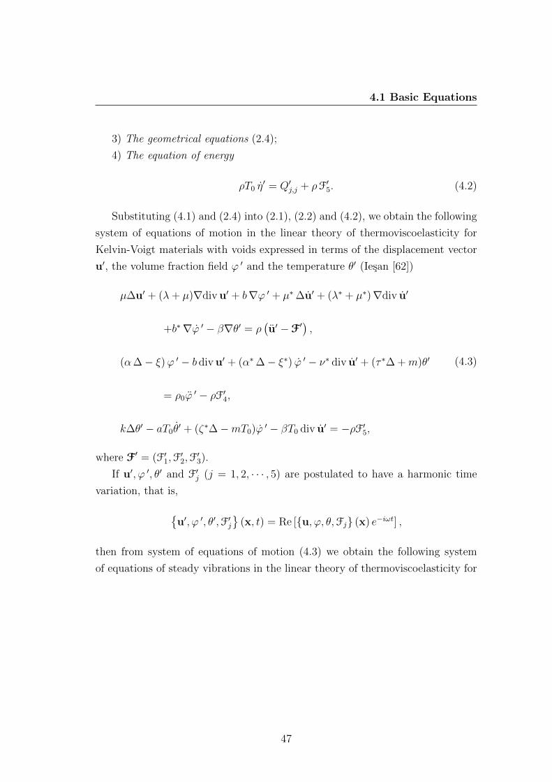
4.1 Basic Equations
3) The geometrical equations (2.4);
4) The equation of energy
ρT0 η′ = Q′j,j + ρF′5. (4.2)
Substituting (4.1) and (2.4) into (2.1), (2.2) and (4.2), we obtain the following
system of equations of motion in the linear theory of thermoviscoelasticity for
Kelvin-Voigt materials with voids expressed in terms of the displacement vector
u′, the volume fraction field ϕ ′ and the temperature θ′ (Iesan [62])
µ∆u′ + (λ+ µ)∇div u′ + b∇ϕ ′ + µ∗∆u′ + (λ∗ + µ∗)∇div u′
+b∗∇ϕ ′ − β∇θ′ = ρ(u′ −F′
),
(α∆− ξ)ϕ ′ − b div u′ + (α∗∆− ξ∗) ϕ ′ − ν∗ div u′ + (τ ∗∆ +m)θ′
= ρ0ϕ′ − ρF′4,
k∆θ′ − aT0θ′ + (ζ∗∆−mT0)ϕ ′ − βT0 div u′ = −ρF′5,
(4.3)
where F′ = (F′1,F′2,F
′3).
If u′, ϕ ′, θ′ and F′j (j = 1, 2, · · · , 5) are postulated to have a harmonic time
variation, that is,
u′, ϕ ′, θ′,F′j
(x, t) = Re [u, ϕ, θ,Fj (x) e−iωt] ,
then from system of equations of motion (4.3) we obtain the following system
of equations of steady vibrations in the linear theory of thermoviscoelasticity for
47
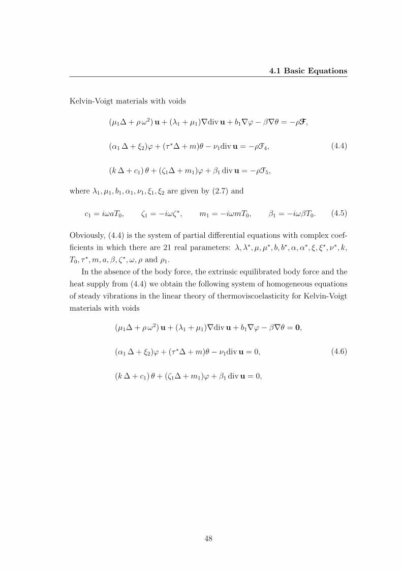
4.1 Basic Equations
Kelvin-Voigt materials with voids
(µ1∆ + ρω2) u + (λ1 + µ1)∇div u + b1∇ϕ− β∇θ = −ρF,
(α1 ∆ + ξ2)ϕ+ (τ ∗∆ +m)θ − ν1div u = −ρF4,
(k∆ + c1) θ + (ζ1∆ +m1)ϕ+ β1 div u = −ρF5,
(4.4)
where λ1, µ1, b1, α1, ν1, ξ1, ξ2 are given by (2.7) and
c1 = iωaT0, ζ1 = −iωζ∗, m1 = −iωmT0, β1 = −iωβT0. (4.5)
Obviously, (4.4) is the system of partial differential equations with complex coef-
ficients in which there are 21 real parameters: λ, λ∗, µ, µ∗, b, b∗, α, α∗, ξ, ξ∗, ν∗, k,
T0, τ∗,m, a, β, ζ∗, ω, ρ and ρ1.
In the absence of the body force, the extrinsic equilibrated body force and the
heat supply from (4.4) we obtain the following system of homogeneous equations
of steady vibrations in the linear theory of thermoviscoelasticity for Kelvin-Voigt
materials with voids
(µ1∆ + ρω2) u + (λ1 + µ1)∇div u + b1∇ϕ− β∇θ = 0,
(α1 ∆ + ξ2)ϕ+ (τ ∗∆ +m)θ − ν1div u = 0,
(k∆ + c1) θ + (ζ1∆ +m1)ϕ+ β1 div u = 0,
(4.6)
48
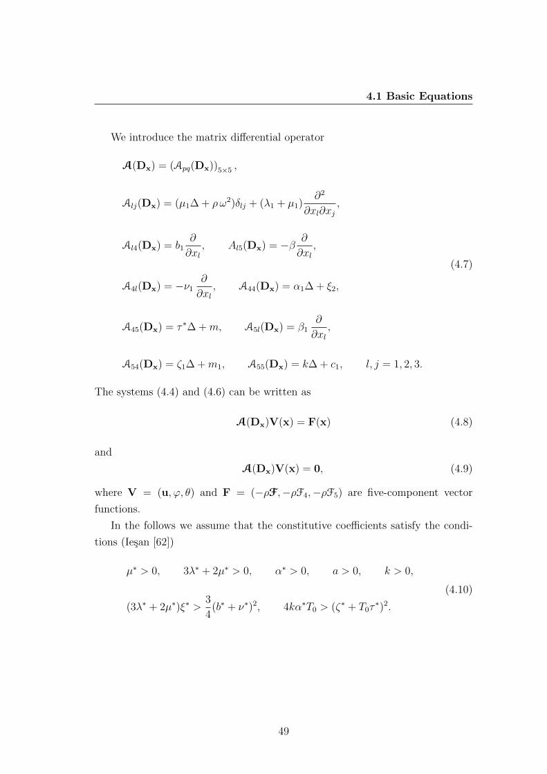
4.1 Basic Equations
We introduce the matrix differential operator
A(Dx) = (Apq(Dx))5×5 ,
Alj(Dx) = (µ1∆ + ρω2)δlj + (λ1 + µ1)∂2
∂xl∂xj,
Al4(Dx) = b1∂
∂xl, Al5(Dx) = −β ∂
∂xl,
A4l(Dx) = −ν1∂
∂xl, A44(Dx) = α1∆ + ξ2,
A45(Dx) = τ ∗∆ +m, A5l(Dx) = β1∂
∂xl,
A54(Dx) = ζ1∆ +m1, A55(Dx) = k∆ + c1, l, j = 1, 2, 3.
(4.7)
The systems (4.4) and (4.6) can be written as
A(Dx)V(x) = F(x) (4.8)
and
A(Dx)V(x) = 0, (4.9)
where V = (u, ϕ, θ) and F = (−ρF,−ρF4,−ρF5) are five-component vector
functions.
In the follows we assume that the constitutive coefficients satisfy the condi-
tions (Iesan [62])
µ∗ > 0, 3λ∗ + 2µ∗ > 0, α∗ > 0, a > 0, k > 0,
(3λ∗ + 2µ∗)ξ∗ >3
4(b∗ + ν∗)2, 4kα∗T0 > (ζ∗ + T0τ
∗)2.
(4.10)
49
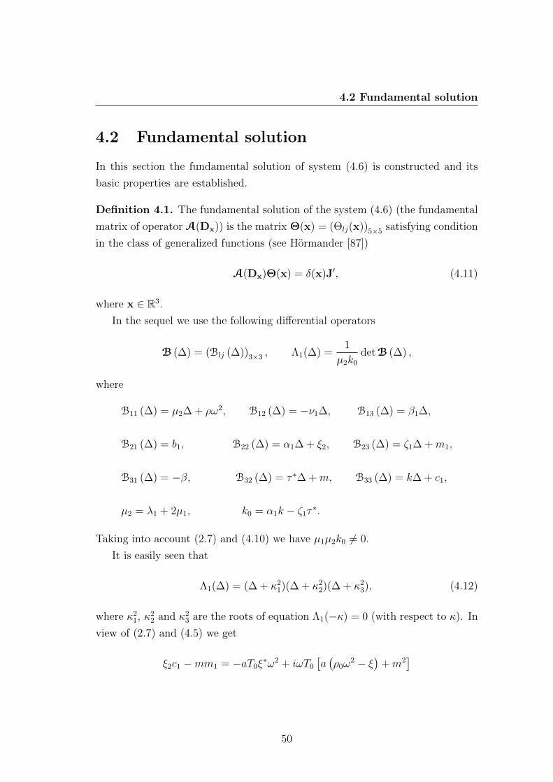
4.2 Fundamental solution
4.2 Fundamental solution
In this section the fundamental solution of system (4.6) is constructed and its
basic properties are established.
Definition 4.1. The fundamental solution of the system (4.6) (the fundamental
matrix of operator A(Dx)) is the matrix Θ(x) = (Θlj(x))5×5 satisfying condition
in the class of generalized functions (see Hormander [87])
A(Dx)Θ(x) = δ(x)J′, (4.11)
where x ∈ R3.
In the sequel we use the following differential operators
B (∆) = (Blj (∆))3×3 , Λ1(∆) =1
µ2k0
detB (∆) ,
where
B11 (∆) = µ2∆ + ρω2, B12 (∆) = −ν1∆, B13 (∆) = β1∆,
B21 (∆) = b1, B22 (∆) = α1∆ + ξ2, B23 (∆) = ζ1∆ +m1,
B31 (∆) = −β, B32 (∆) = τ ∗∆ +m, B33 (∆) = k∆ + c1,
µ2 = λ1 + 2µ1, k0 = α1k − ζ1τ∗.
Taking into account (2.7) and (4.10) we have µ1µ2k0 6= 0.
It is easily seen that
Λ1(∆) = (∆ + κ21)(∆ + κ2
2)(∆ + κ23), (4.12)
where κ21, κ
22 and κ2
3 are the roots of equation Λ1(−κ) = 0 (with respect to κ). In
view of (2.7) and (4.5) we get
ξ2c1 −mm1 = −aT0ξ∗ω2 + iωT0
[a(ρ0ω
2 − ξ)
+m2]
50
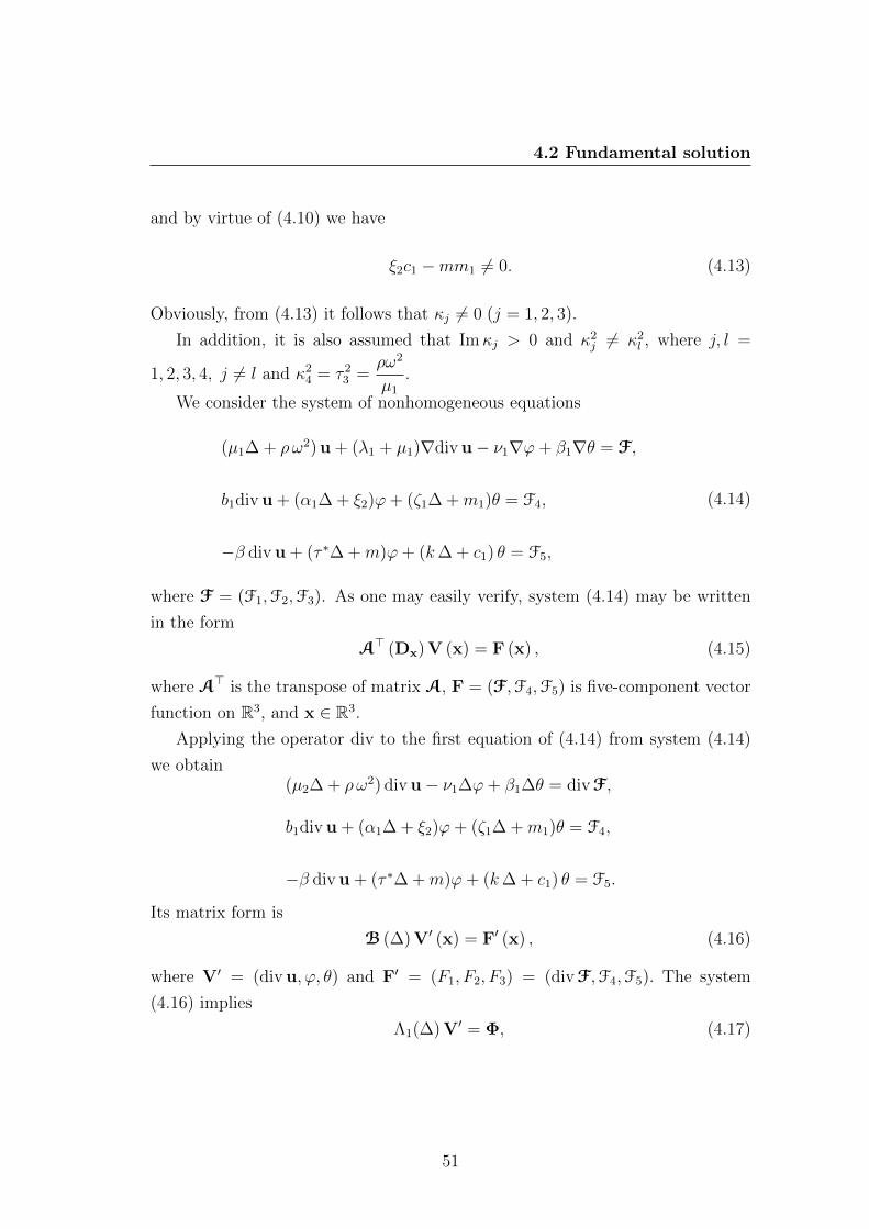
4.2 Fundamental solution
and by virtue of (4.10) we have
ξ2c1 −mm1 6= 0. (4.13)
Obviously, from (4.13) it follows that κj 6= 0 (j = 1, 2, 3).
In addition, it is also assumed that Imκj > 0 and κ2j 6= κ2
l , where j, l =
1, 2, 3, 4, j 6= l and κ24 = τ 2
3 =ρω2
µ1
.
We consider the system of nonhomogeneous equations
(µ1∆ + ρω2) u + (λ1 + µ1)∇div u− ν1∇ϕ+ β1∇θ = F,
b1div u + (α1∆ + ξ2)ϕ+ (ζ1∆ +m1)θ = F4,
−β div u + (τ ∗∆ +m)ϕ+ (k∆ + c1) θ = F5,
(4.14)
where F = (F1,F2,F3). As one may easily verify, system (4.14) may be written
in the form
A> (Dx) V (x) = F (x) , (4.15)
where A> is the transpose of matrix A, F = (F,F4,F5) is five-component vector
function on R3, and x ∈ R3.
Applying the operator div to the first equation of (4.14) from system (4.14)
we obtain(µ2∆ + ρω2) div u− ν1∆ϕ+ β1∆θ = divF,
b1div u + (α1∆ + ξ2)ϕ+ (ζ1∆ +m1)θ = F4,
−β div u + (τ ∗∆ +m)ϕ+ (k∆ + c1) θ = F5.
Its matrix form is
B (∆) V′ (x) = F′ (x) , (4.16)
where V′ = (div u, ϕ, θ) and F′ = (F1, F2, F3) = (divF,F4,F5). The system
(4.16) implies
Λ1(∆) V′ = Φ, (4.17)
51
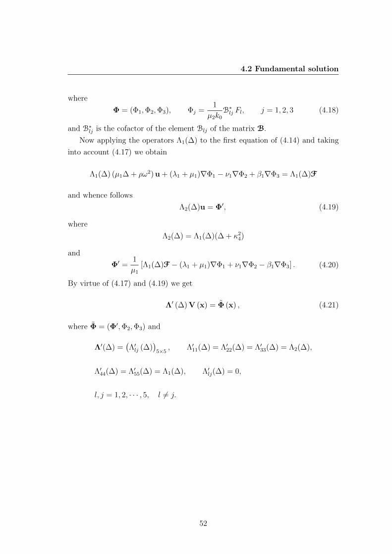
4.2 Fundamental solution
where
Φ = (Φ1,Φ2,Φ3), Φj =1
µ2k0
B∗lj Fl, j = 1, 2, 3 (4.18)
and B∗lj is the cofactor of the element Blj of the matrix B.
Now applying the operators Λ1(∆) to the first equation of (4.14) and taking
into account (4.17) we obtain
Λ1(∆) (µ1∆ + ρω2) u + (λ1 + µ1)∇Φ1 − ν1∇Φ2 + β1∇Φ3 = Λ1(∆)F
and whence follows
Λ2(∆)u = Φ′, (4.19)
where
Λ2(∆) = Λ1(∆)(∆ + κ24)
and
Φ′ =1
µ1
[Λ1(∆)F− (λ1 + µ1)∇Φ1 + ν1∇Φ2 − β1∇Φ3] . (4.20)
By virtue of (4.17) and (4.19) we get
Λ′ (∆) V (x) = Φ (x) , (4.21)
where Φ = (Φ′,Φ2,Φ3) and
Λ′(∆) =(Λ′lj (∆)
)5×5
, Λ′11(∆) = Λ′22(∆) = Λ′33(∆) = Λ2(∆),
Λ′44(∆) = Λ′55(∆) = Λ1(∆), Λ′lj(∆) = 0,
l, j = 1, 2, · · · , 5, l 6= j.
52
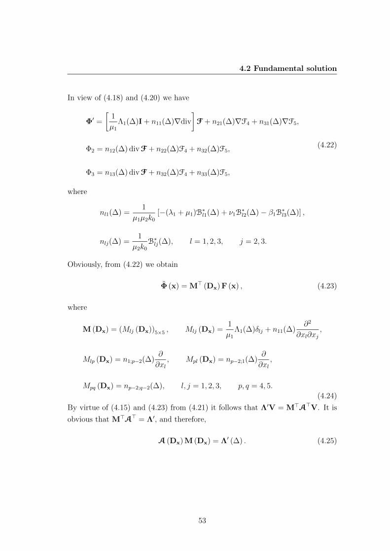
4.2 Fundamental solution
In view of (4.18) and (4.20) we have
Φ′ =
[1
µ1
Λ1(∆)I + n11(∆)∇div
]F + n21(∆)∇F4 + n31(∆)∇F5,
Φ2 = n12(∆) divF + n22(∆)F4 + n32(∆)F5,
Φ3 = n13(∆) divF + n32(∆)F4 + n33(∆)F5,
(4.22)
where
nl1(∆) =1
µ1µ2k0
[−(λ1 + µ1)B∗l1(∆) + ν1B∗l2(∆)− β1B
∗l3(∆)] ,
nlj(∆) =1
µ2k0
B∗lj(∆), l = 1, 2, 3, j = 2, 3.
Obviously, from (4.22) we obtain
Φ (x) = M> (Dx) F (x) , (4.23)
where
M (Dx) = (Mlj (Dx))5×5 , Mlj (Dx) =1
µ1
Λ1(∆)δlj + n11(∆)∂2
∂xl∂xj,
Mlp (Dx) = n1;p−2(∆)∂
∂xl, Mpl (Dx) = np−2;1(∆)
∂
∂xl,
Mpq (Dx) = np−2;q−2(∆), l, j = 1, 2, 3, p, q = 4, 5.
(4.24)
By virtue of (4.15) and (4.23) from (4.21) it follows that Λ′V = M>A>V. It is
obvious that M>A> = Λ′, and therefore,
A (Dx) M (Dx) = Λ′ (∆) . (4.25)
53
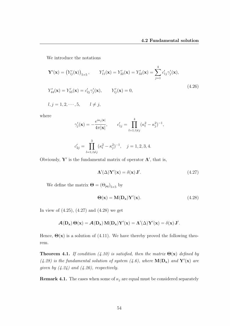
4.2 Fundamental solution
We introduce the notations
Y′(x) =(Y ′lj(x)
)5×5
, Y ′11(x) = Y ′22(x) = Y ′33(x) =4∑j=1
c′1jγ′j(x),
Y ′44(x) = Y ′55(x) = c′2jγ′j(x), Y ′lj(x) = 0,
l, j = 1, 2, · · · , 5, l 6= j,
(4.26)
where
γ′j(x) = −eiκj |x|
4π|x|, c′1j =
4∏l=1; l 6=j
(κ2l − κ2
j)−1,
c′2j =3∏
l=1; l 6=j
(κ2l − κ2
j)−1, j = 1, 2, 3, 4.
Obviously, Y′ is the fundamental matrix of operator Λ′, that is,
Λ′(∆)Y′(x) = δ(x) J′. (4.27)
We define the matrix Θ = (Θpq)5×5 by
Θ(x) = M(Dx)Y′(x). (4.28)
In view of (4.25), (4.27) and (4.28) we get
A(Dx) Θ(x) = A(Dx) M(Dx)Y′(x) = Λ′(∆)Y′(x) = δ(x) J′.
Hence, Θ(x) is a solution of (4.11). We have thereby proved the following theo-
rem.
Theorem 4.1. If condition (4.10) is satisfied, then the matrix Θ(x) defined by
(4.28) is the fundamental solution of system (4.6), where M(Dx) and Y′(x) are
given by (4.24) and (4.26), respectively.
Remark 4.1. The cases when some of κj are equal must be considered separately
54
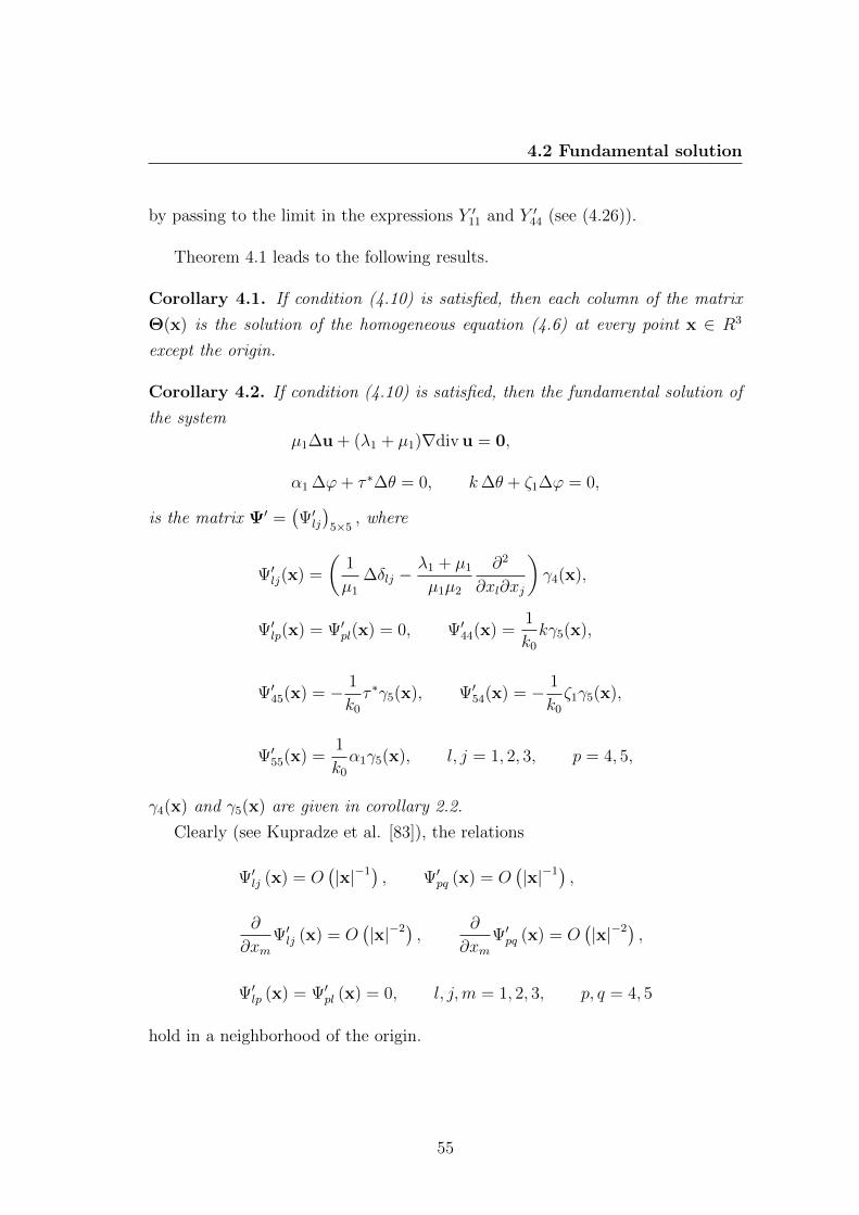
4.2 Fundamental solution
by passing to the limit in the expressions Y ′11 and Y ′44 (see (4.26)).
Theorem 4.1 leads to the following results.
Corollary 4.1. If condition (4.10) is satisfied, then each column of the matrix
Θ(x) is the solution of the homogeneous equation (4.6) at every point x ∈ R3
except the origin.
Corollary 4.2. If condition (4.10) is satisfied, then the fundamental solution of
the system
µ1∆u + (λ1 + µ1)∇div u = 0,
α1 ∆ϕ+ τ ∗∆θ = 0, k∆θ + ζ1∆ϕ = 0,
is the matrix Ψ′ =(Ψ′lj)
5×5, where
Ψ′lj(x) =
(1
µ1
∆δlj −λ1 + µ1
µ1µ2
∂2
∂xl∂xj
)γ4(x),
Ψ′lp(x) = Ψ′pl(x) = 0, Ψ′44(x) =1
k0
kγ5(x),
Ψ′45(x) = − 1
k0
τ ∗γ5(x), Ψ′54(x) = − 1
k0
ζ1γ5(x),
Ψ′55(x) =1
k0
α1γ5(x), l, j = 1, 2, 3, p = 4, 5,
γ4(x) and γ5(x) are given in corollary 2.2.
Clearly (see Kupradze et al. [83]), the relations
Ψ′lj (x) = O(|x|−1) , Ψ′pq (x) = O
(|x|−1) ,
∂
∂xmΨ′lj (x) = O
(|x|−2) , ∂
∂xmΨ′pq (x) = O
(|x|−2) ,
Ψ′lp (x) = Ψ′pl (x) = 0, l, j,m = 1, 2, 3, p, q = 4, 5
hold in a neighborhood of the origin.
55
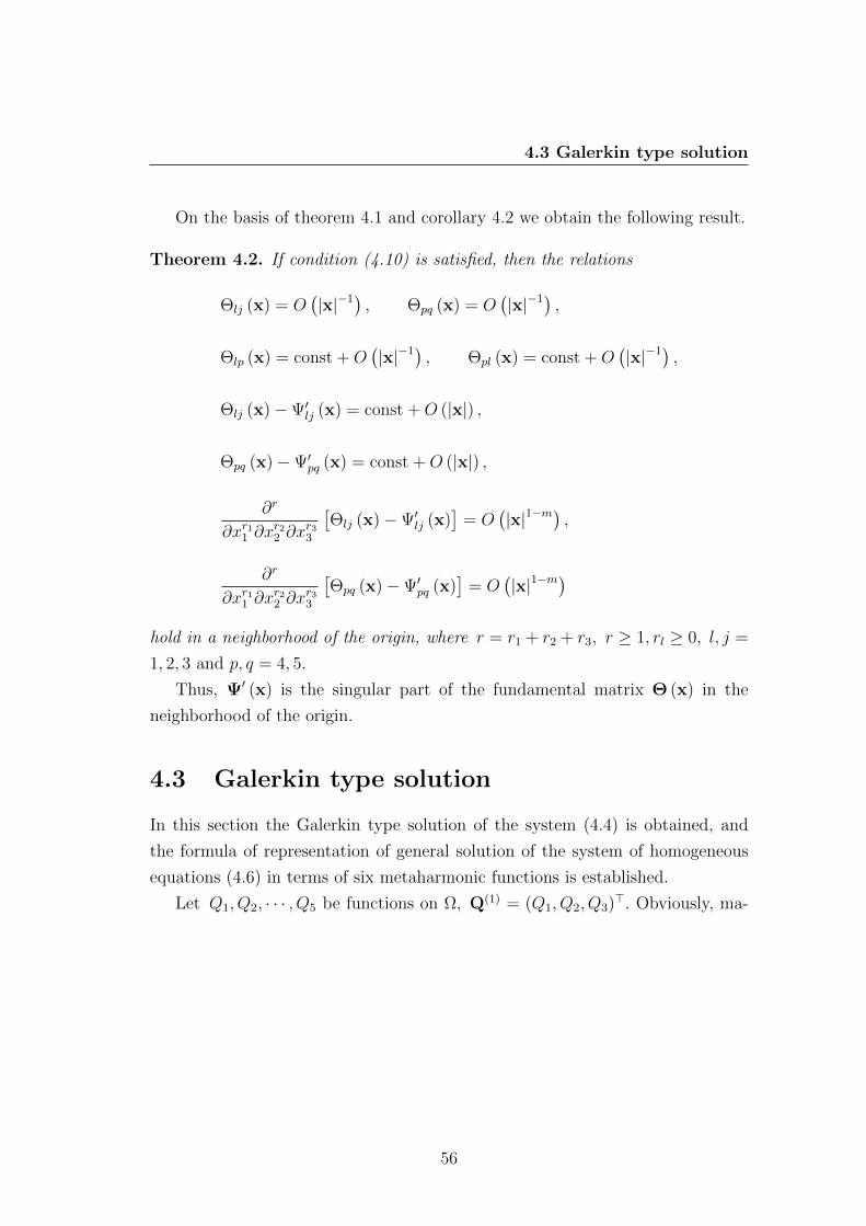
4.3 Galerkin type solution
On the basis of theorem 4.1 and corollary 4.2 we obtain the following result.
Theorem 4.2. If condition (4.10) is satisfied, then the relations
Θlj (x) = O(|x|−1) , Θpq (x) = O
(|x|−1) ,
Θlp (x) = const +O(|x|−1) , Θpl (x) = const +O
(|x|−1) ,
Θlj (x)−Ψ′lj (x) = const +O (|x|) ,
Θpq (x)−Ψ′pq (x) = const +O (|x|) ,
∂r
∂xr11 ∂xr22 ∂x
r33
[Θlj (x)−Ψ′lj (x)
]= O
(|x|1−m
),
∂r
∂xr11 ∂xr22 ∂x
r33
[Θpq (x)−Ψ′pq (x)
]= O
(|x|1−m
)hold in a neighborhood of the origin, where r = r1 + r2 + r3, r ≥ 1, rl ≥ 0, l, j =
1, 2, 3 and p, q = 4, 5.
Thus, Ψ′ (x) is the singular part of the fundamental matrix Θ (x) in the
neighborhood of the origin.
4.3 Galerkin type solution
In this section the Galerkin type solution of the system (4.4) is obtained, and
the formula of representation of general solution of the system of homogeneous
equations (4.6) in terms of six metaharmonic functions is established.
Let Q1, Q2, · · · , Q5 be functions on Ω, Q(1) = (Q1, Q2, Q3)>. Obviously, ma-
56
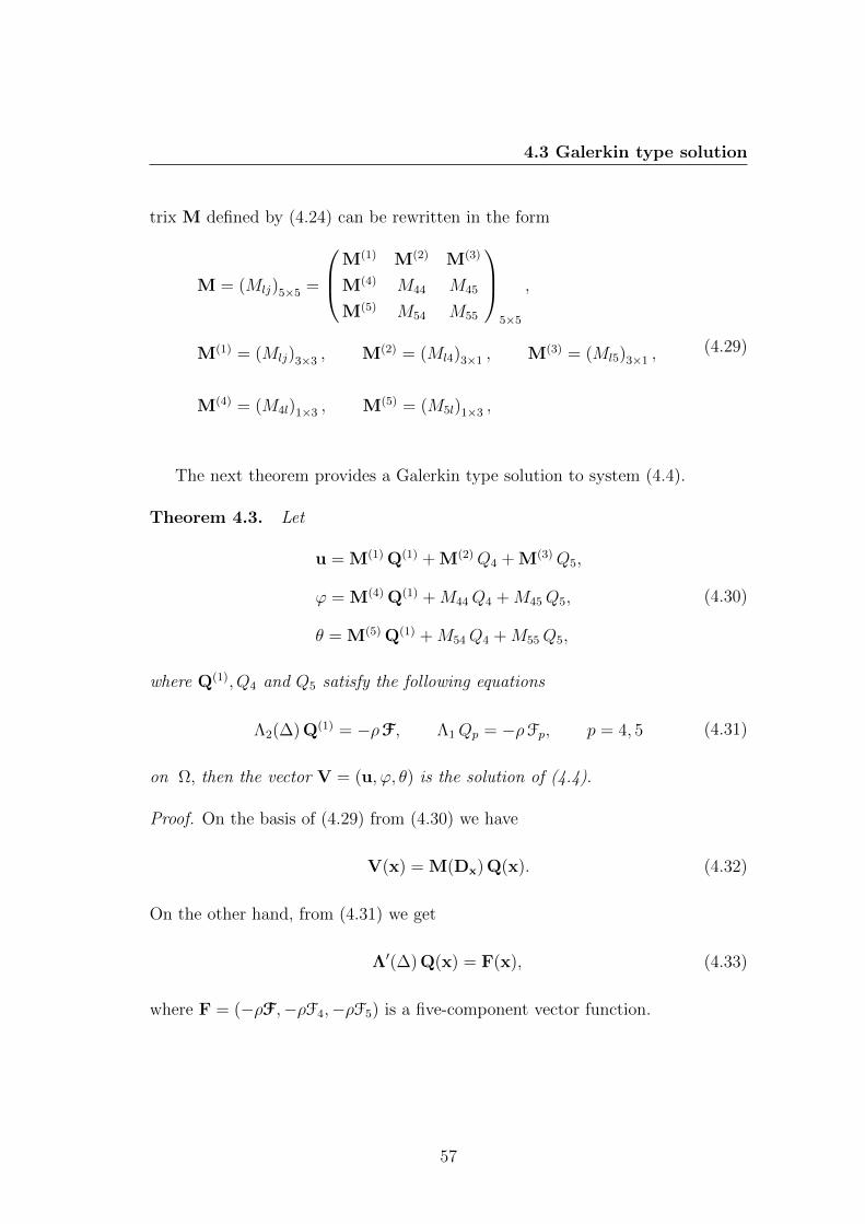
4.3 Galerkin type solution
trix M defined by (4.24) can be rewritten in the form
M = (Mlj)5×5 =
M(1) M(2) M(3)
M(4) M44 M45
M(5) M54 M55
5×5
,
M(1) = (Mlj)3×3 , M(2) = (Ml4)3×1 , M(3) = (Ml5)3×1 ,
M(4) = (M4l)1×3 , M(5) = (M5l)1×3 ,
(4.29)
The next theorem provides a Galerkin type solution to system (4.4).
Theorem 4.3. Let
u = M(1) Q(1) + M(2)Q4 + M(3) Q5,
ϕ = M(4) Q(1) +M44Q4 +M45Q5,
θ = M(5) Q(1) +M54Q4 +M55Q5,
(4.30)
where Q(1), Q4 and Q5 satisfy the following equations
Λ2(∆) Q(1) = −ρF, Λ1Qp = −ρFp, p = 4, 5 (4.31)
on Ω, then the vector V = (u, ϕ, θ) is the solution of (4.4).
Proof. On the basis of (4.29) from (4.30) we have
V(x) = M(Dx) Q(x). (4.32)
On the other hand, from (4.31) we get
Λ′(∆) Q(x) = F(x), (4.33)
where F = (−ρF,−ρF4,−ρF5) is a five-component vector function.
57
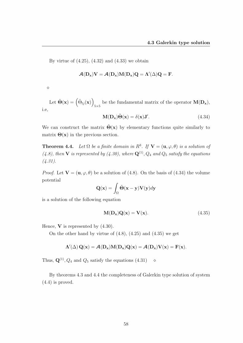
4.3 Galerkin type solution
By virtue of (4.25), (4.32) and (4.33) we obtain
A(Dx)V = A(Dx)M(Dx)Q = Λ′(∆)Q = F.
Let Θ(x) =(
Θlj(x))
5×5be the fundamental matrix of the operator M(Dx),
i.e,
M(Dx)Θ(x) = δ(x)J′. (4.34)
We can construct the matrix Θ(x) by elementary functions quite similarly to
matrix Θ(x) in the previous section.
Theorem 4.4. Let Ω be a finite domain in R3. If V = (u, ϕ, θ) is a solution of
(4.8), then V is represented by (4.30), where Q(1), Q4 and Q5 satisfy the equations
(4.31).
Proof. Let V = (u, ϕ, θ) be a solution of (4.8). On the basis of (4.34) the volume
potential
Q(x) =
∫Ω
Θ(x− y)V(y)dy
is a solution of the following equation
M(Dx)Q(x) = V(x). (4.35)
Hence, V is represented by (4.30).
On the other hand by virtue of (4.8), (4.25) and (4.35) we get
Λ′(∆) Q(x) = A(Dx)M(Dx)Q(x) = A(Dx)V(x) = F(x).
Thus, Q(1), Q4 and Q5 satisfy the equations (4.31)
By theorems 4.3 and 4.4 the completeness of Galerkin type solution of system
(4.4) is proved.
58
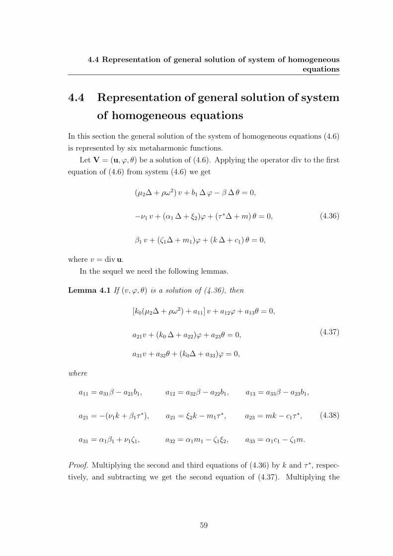
4.4 Representation of general solution of system of homogeneousequations
4.4 Representation of general solution of system
of homogeneous equations
In this section the general solution of the system of homogeneous equations (4.6)
is represented by six metaharmonic functions.
Let V = (u, ϕ, θ) be a solution of (4.6). Applying the operator div to the first
equation of (4.6) from system (4.6) we get
(µ2∆ + ρω2) v + b1 ∆ϕ− β∆ θ = 0,
−ν1 v + (α1 ∆ + ξ2)ϕ+ (τ ∗∆ +m) θ = 0,
β1 v + (ζ1∆ +m1)ϕ+ (k∆ + c1) θ = 0,
(4.36)
where v = div u.
In the sequel we need the following lemmas.
Lemma 4.1 If (v, ϕ, θ) is a solution of (4.36), then
[k0(µ2∆ + ρω2) + a11] v + a12ϕ+ a13θ = 0,
a21v + (k0 ∆ + a22)ϕ+ a23θ = 0,
a31v + a32θ + (k0∆ + a33)ϕ = 0,
(4.37)
where
a11 = a31β − a21b1, a12 = a32β − a22b1, a13 = a33β − a23b1,
a21 = −(ν1k + β1τ∗), a21 = ξ2k −m1τ
∗, a23 = mk − c1τ∗,
a31 = α1β1 + ν1ζ1, a32 = α1m1 − ζ1ξ2, a33 = α1c1 − ζ1m.
(4.38)
Proof. Multiplying the second and third equations of (4.36) by k and τ ∗, respec-
tively, and subtracting we get the second equation of (4.37). Multiplying the
59
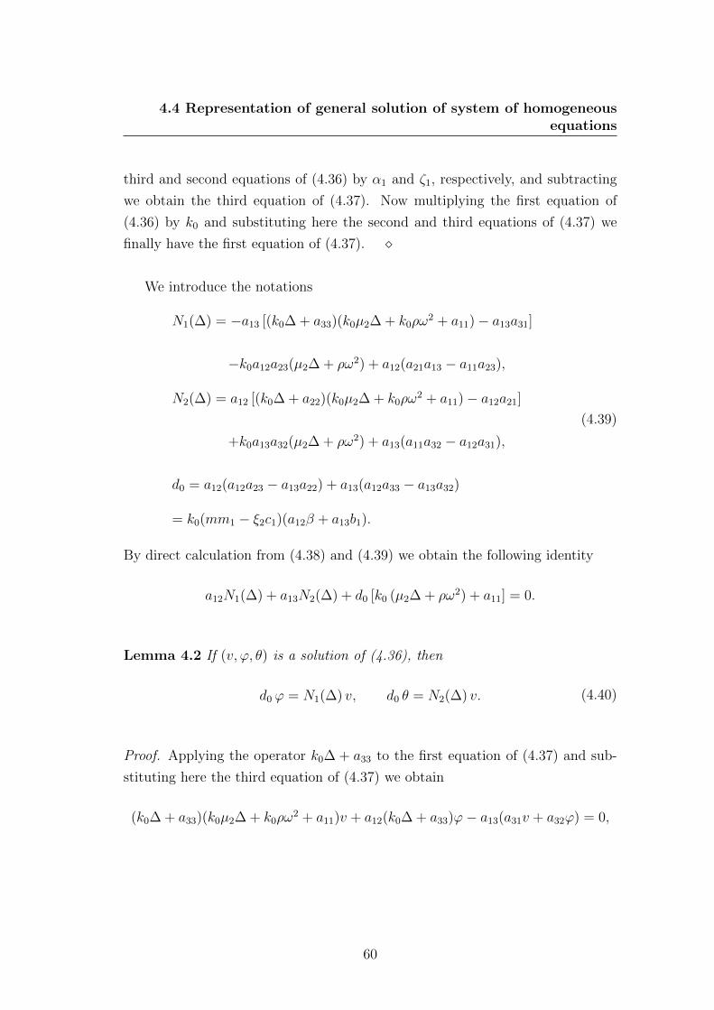
4.4 Representation of general solution of system of homogeneousequations
third and second equations of (4.36) by α1 and ζ1, respectively, and subtracting
we obtain the third equation of (4.37). Now multiplying the first equation of
(4.36) by k0 and substituting here the second and third equations of (4.37) we
finally have the first equation of (4.37).
We introduce the notations
N1(∆) = −a13 [(k0∆ + a33)(k0µ2∆ + k0ρω2 + a11)− a13a31]
−k0a12a23(µ2∆ + ρω2) + a12(a21a13 − a11a23),
N2(∆) = a12 [(k0∆ + a22)(k0µ2∆ + k0ρω2 + a11)− a12a21]
+k0a13a32(µ2∆ + ρω2) + a13(a11a32 − a12a31),
d0 = a12(a12a23 − a13a22) + a13(a12a33 − a13a32)
= k0(mm1 − ξ2c1)(a12β + a13b1).
(4.39)
By direct calculation from (4.38) and (4.39) we obtain the following identity
a12N1(∆) + a13N2(∆) + d0 [k0 (µ2∆ + ρω2) + a11] = 0.
Lemma 4.2 If (v, ϕ, θ) is a solution of (4.36), then
d0 ϕ = N1(∆) v, d0 θ = N2(∆) v. (4.40)
Proof. Applying the operator k0∆ + a33 to the first equation of (4.37) and sub-
stituting here the third equation of (4.37) we obtain
(k0∆ + a33)(k0µ2∆ + k0ρω2 + a11)v + a12(k0∆ + a33)ϕ− a13(a31v + a32ϕ) = 0,
60
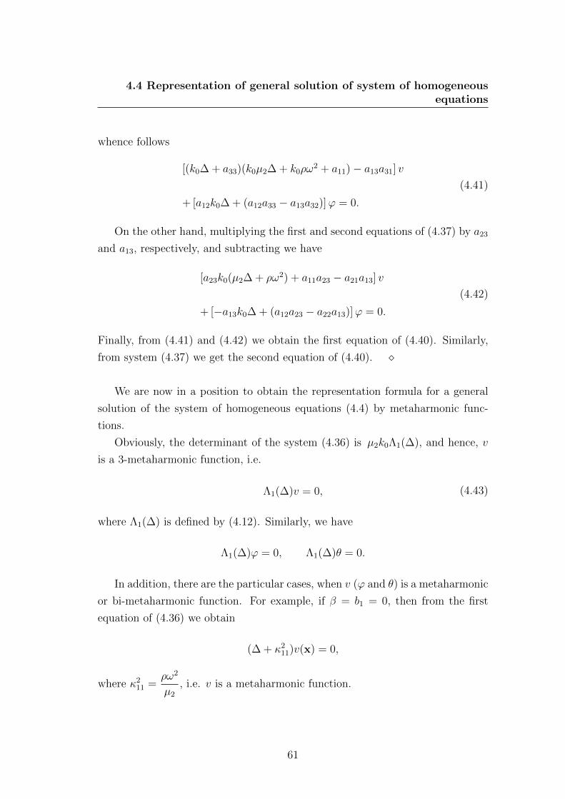
4.4 Representation of general solution of system of homogeneousequations
whence follows
[(k0∆ + a33)(k0µ2∆ + k0ρω2 + a11)− a13a31] v
+ [a12k0∆ + (a12a33 − a13a32)]ϕ = 0.
(4.41)
On the other hand, multiplying the first and second equations of (4.37) by a23
and a13, respectively, and subtracting we have
[a23k0(µ2∆ + ρω2) + a11a23 − a21a13] v
+ [−a13k0∆ + (a12a23 − a22a13)]ϕ = 0.
(4.42)
Finally, from (4.41) and (4.42) we obtain the first equation of (4.40). Similarly,
from system (4.37) we get the second equation of (4.40).
We are now in a position to obtain the representation formula for a general
solution of the system of homogeneous equations (4.4) by metaharmonic func-
tions.
Obviously, the determinant of the system (4.36) is µ2k0Λ1(∆), and hence, v
is a 3-metaharmonic function, i.e.
Λ1(∆)v = 0, (4.43)
where Λ1(∆) is defined by (4.12). Similarly, we have
Λ1(∆)ϕ = 0, Λ1(∆)θ = 0.
In addition, there are the particular cases, when v (ϕ and θ) is a metaharmonic
or bi-metaharmonic function. For example, if β = b1 = 0, then from the first
equation of (4.36) we obtain
(∆ + κ211)v(x) = 0,
where κ211 =
ρω2
µ2
, i.e. v is a metaharmonic function.
61
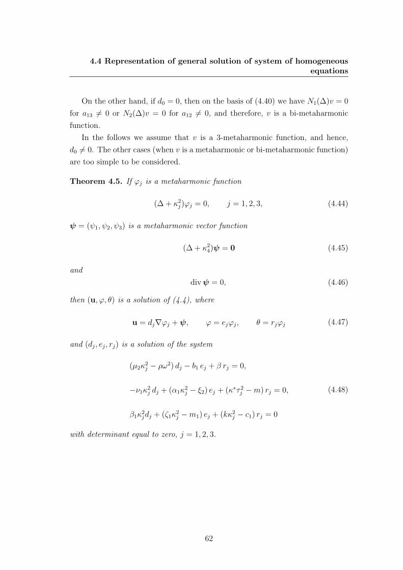
4.4 Representation of general solution of system of homogeneousequations
On the other hand, if d0 = 0, then on the basis of (4.40) we have N1(∆)v = 0
for a13 6= 0 or N2(∆)v = 0 for a12 6= 0, and therefore, v is a bi-metaharmonic
function.
In the follows we assume that v is a 3-metaharmonic function, and hence,
d0 6= 0. The other cases (when v is a metaharmonic or bi-metaharmonic function)
are too simple to be considered.
Theorem 4.5. If ϕj is a metaharmonic function
(∆ + κ2j)ϕj = 0, j = 1, 2, 3, (4.44)
ψ = (ψ1, ψ2, ψ3) is a metaharmonic vector function
(∆ + κ24)ψ = 0 (4.45)
and
divψ = 0, (4.46)
then (u, ϕ, θ) is a solution of (4.4), where
u = dj∇ϕj +ψ, ϕ = ejϕj, θ = rjϕj (4.47)
and (dj, ej, rj) is a solution of the system
(µ2κ2j − ρω2) dj − b1 ej + β rj = 0,
−ν1κ2j dj + (α1κ
2j − ξ2) ej + (κ∗τ 2
j −m) rj = 0,
β1κ2jdj + (ζ1κ
2j −m1) ej + (kκ2
j − c1) rj = 0
(4.48)
with determinant equal to zero, j = 1, 2, 3.
62
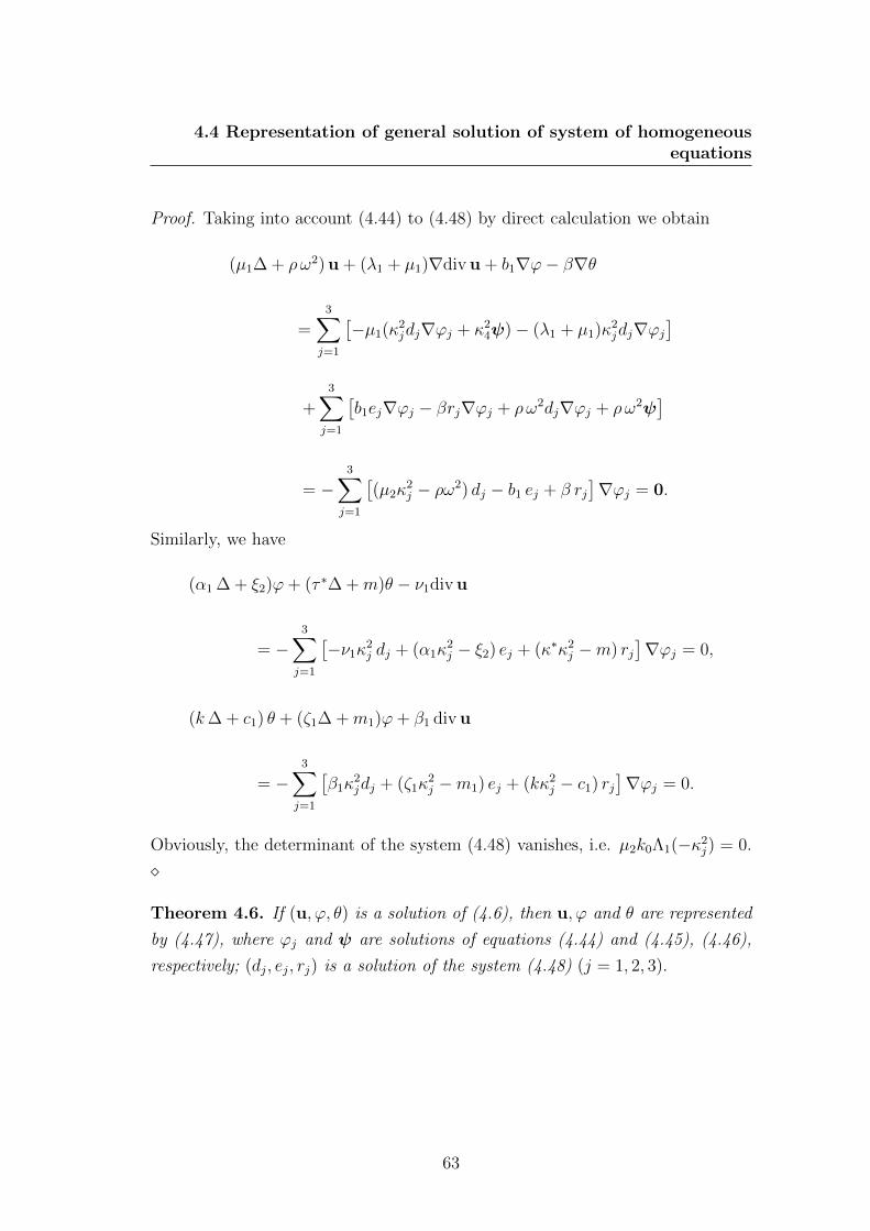
4.4 Representation of general solution of system of homogeneousequations
Proof. Taking into account (4.44) to (4.48) by direct calculation we obtain
(µ1∆ + ρω2) u + (λ1 + µ1)∇div u + b1∇ϕ− β∇θ
=3∑j=1
[−µ1(κ2
jdj∇ϕj + κ24ψ)− (λ1 + µ1)κ2
jdj∇ϕj]
+3∑j=1
[b1ej∇ϕj − βrj∇ϕj + ρω2dj∇ϕj + ρω2ψ
]
= −3∑j=1
[(µ2κ
2j − ρω2) dj − b1 ej + β rj
]∇ϕj = 0.
Similarly, we have
(α1 ∆ + ξ2)ϕ+ (τ ∗∆ +m)θ − ν1div u
= −3∑j=1
[−ν1κ
2j dj + (α1κ
2j − ξ2) ej + (κ∗κ2
j −m) rj]∇ϕj = 0,
(k∆ + c1) θ + (ζ1∆ +m1)ϕ+ β1 div u
= −3∑j=1
[β1κ
2jdj + (ζ1κ
2j −m1) ej + (kκ2
j − c1) rj]∇ϕj = 0.
Obviously, the determinant of the system (4.48) vanishes, i.e. µ2k0Λ1(−κ2j) = 0.
Theorem 4.6. If (u, ϕ, θ) is a solution of (4.6), then u, ϕ and θ are represented
by (4.47), where ϕj and ψ are solutions of equations (4.44) and (4.45), (4.46),
respectively; (dj, ej, rj) is a solution of the system (4.48) (j = 1, 2, 3).
63
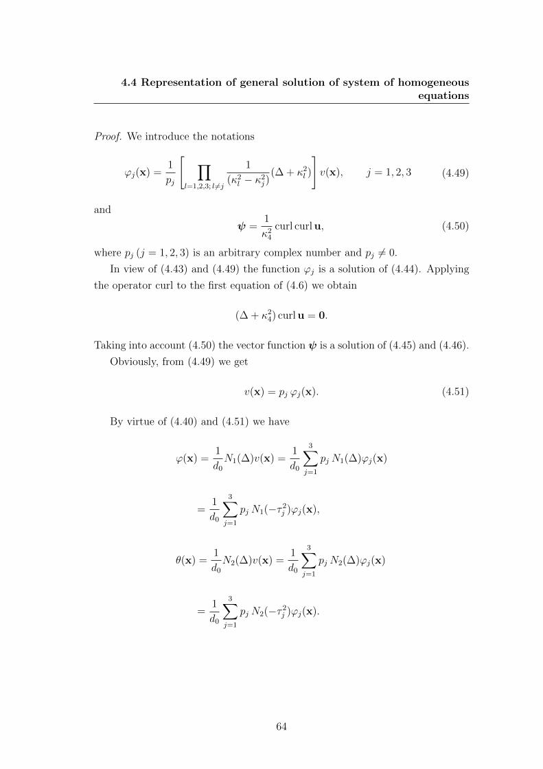
4.4 Representation of general solution of system of homogeneousequations
Proof. We introduce the notations
ϕj(x) =1
pj
[ ∏l=1,2,3; l 6=j
1
(κ2l − κ2
j)(∆ + κ2
l )
]v(x), j = 1, 2, 3 (4.49)
and
ψ =1
κ24
curl curl u, (4.50)
where pj (j = 1, 2, 3) is an arbitrary complex number and pj 6= 0.
In view of (4.43) and (4.49) the function ϕj is a solution of (4.44). Applying
the operator curl to the first equation of (4.6) we obtain
(∆ + κ24) curl u = 0.
Taking into account (4.50) the vector function ψ is a solution of (4.45) and (4.46).
Obviously, from (4.49) we get
v(x) = pj ϕj(x). (4.51)
By virtue of (4.40) and (4.51) we have
ϕ(x) =1
d0
N1(∆)v(x) =1
d0
3∑j=1
pj N1(∆)ϕj(x)
=1
d0
3∑j=1
pj N1(−τ 2j )ϕj(x),
θ(x) =1
d0
N2(∆)v(x) =1
d0
3∑j=1
pj N2(∆)ϕj(x)
=1
d0
3∑j=1
pj N2(−τ 2j )ϕj(x).
64
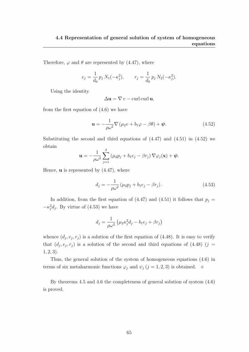
4.4 Representation of general solution of system of homogeneousequations
Therefore, ϕ and θ are represented by (4.47), where
ej =1
d0
pj N1(−κ2j), rj =
1
d0
pj N2(−κ2j).
Using the identity
∆u = ∇ v − curl curl u,
from the first equation of (4.6) we have
u = − 1
ρω2∇ (µ2v + b1ϕ− βθ) +ψ. (4.52)
Substituting the second and third equations of (4.47) and (4.51) in (4.52) we
obtain
u = − 1
ρω2
3∑j=1
(µ2pj + b1ej − βrj)∇ϕj(x) +ψ.
Hence, u is represented by (4.47), where
dj = − 1
ρω2(µ2pj + b1ej − βrj) . (4.53)
In addition, from the first equation of (4.47) and (4.51) it follows that pj =
−κ2jdj. By virtue of (4.53) we have
dj =1
ρω2
(µ2κ
2jdj − b1ej + βrj
)whence (dj, ej, rj) is a solution of the first equation of (4.48). It is easy to verify
that (dj, ej, rj) is a solution of the second and third equations of (4.48) (j =
1, 2, 3).
Thus, the general solution of the system of homogeneous equations (4.6) in
terms of six metaharmonic functions ϕj and ψj (j = 1, 2, 3) is obtained.
By theorems 4.5 and 4.6 the completeness of general solution of system (4.6)
is proved.
65
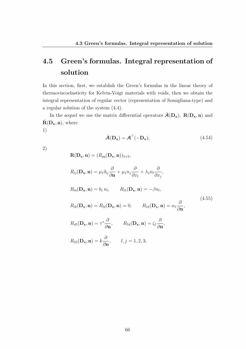
4.3 Green’s formulas. Integral representation of solution
4.5 Green’s formulas. Integral representation of
solution
In this section, first, we establish the Green’s formulas in the linear theory of
thermoviscoelasticity for Kelvin-Voigt materials with voids, then we obtain the
integral representation of regular vector (representation of Somigliana-type) and
a regular solution of the system (4.4).
In the sequel we use the matrix differential operators A(Dx), R(Dx,n) and
R(Dx,n), where
1)
A(Dx) = A>(−Dx); (4.54)
2)
R(Dx,n) = (Rpq(Dx,n))5×5,
Rlj(Dx,n) = µ1δlj∂
∂n+ µ1nj
∂
∂xl+ λ1nl
∂
∂xj,
Rl4(Dx,n) = b1 nl, Rl5(Dx,n) = −βnl,
R4l(Dx,n) = R5l(Dx,n) = 0, R44(Dx,n) = α1∂
∂n,
R45(Dx,n) = τ ∗∂
∂n, R54(Dx,n) = ζ1
∂
∂n,
R55(Dx,n) = k∂
∂n, l, j = 1, 2, 3;
(4.55)
66
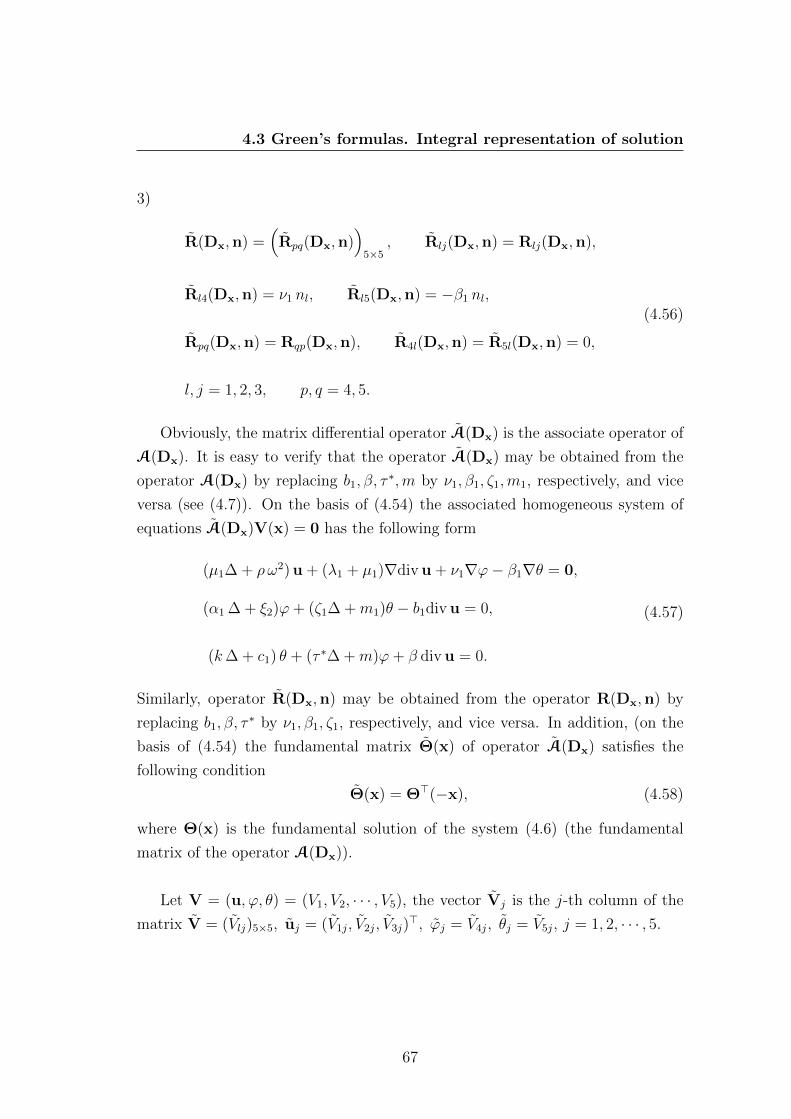
4.3 Green’s formulas. Integral representation of solution
3)
R(Dx,n) =(Rpq(Dx,n)
)5×5
, Rlj(Dx,n) = Rlj(Dx,n),
Rl4(Dx,n) = ν1 nl, Rl5(Dx,n) = −β1 nl,
Rpq(Dx,n) = Rqp(Dx,n), R4l(Dx,n) = R5l(Dx,n) = 0,
l, j = 1, 2, 3, p, q = 4, 5.
(4.56)
Obviously, the matrix differential operator A(Dx) is the associate operator of
A(Dx). It is easy to verify that the operator A(Dx) may be obtained from the
operator A(Dx) by replacing b1, β, τ∗,m by ν1, β1, ζ1,m1, respectively, and vice
versa (see (4.7)). On the basis of (4.54) the associated homogeneous system of
equations A(Dx)V(x) = 0 has the following form
(µ1∆ + ρω2) u + (λ1 + µ1)∇div u + ν1∇ϕ− β1∇θ = 0,
(α1 ∆ + ξ2)ϕ+ (ζ1∆ +m1)θ − b1div u = 0,
(k∆ + c1) θ + (τ ∗∆ +m)ϕ+ β div u = 0.
(4.57)
Similarly, operator R(Dx,n) may be obtained from the operator R(Dx,n) by
replacing b1, β, τ∗ by ν1, β1, ζ1, respectively, and vice versa. In addition, (on the
basis of (4.54) the fundamental matrix Θ(x) of operator A(Dx) satisfies the
following condition
Θ(x) = Θ>(−x), (4.58)
where Θ(x) is the fundamental solution of the system (4.6) (the fundamental
matrix of the operator A(Dx)).
Let V = (u, ϕ, θ) = (V1, V2, · · · , V5), the vector Vj is the j-th column of the
matrix V = (Vlj)5×5, uj = (V1j, V2j, V3j)>, ϕj = V4j, θj = V5j, j = 1, 2, · · · , 5.
67
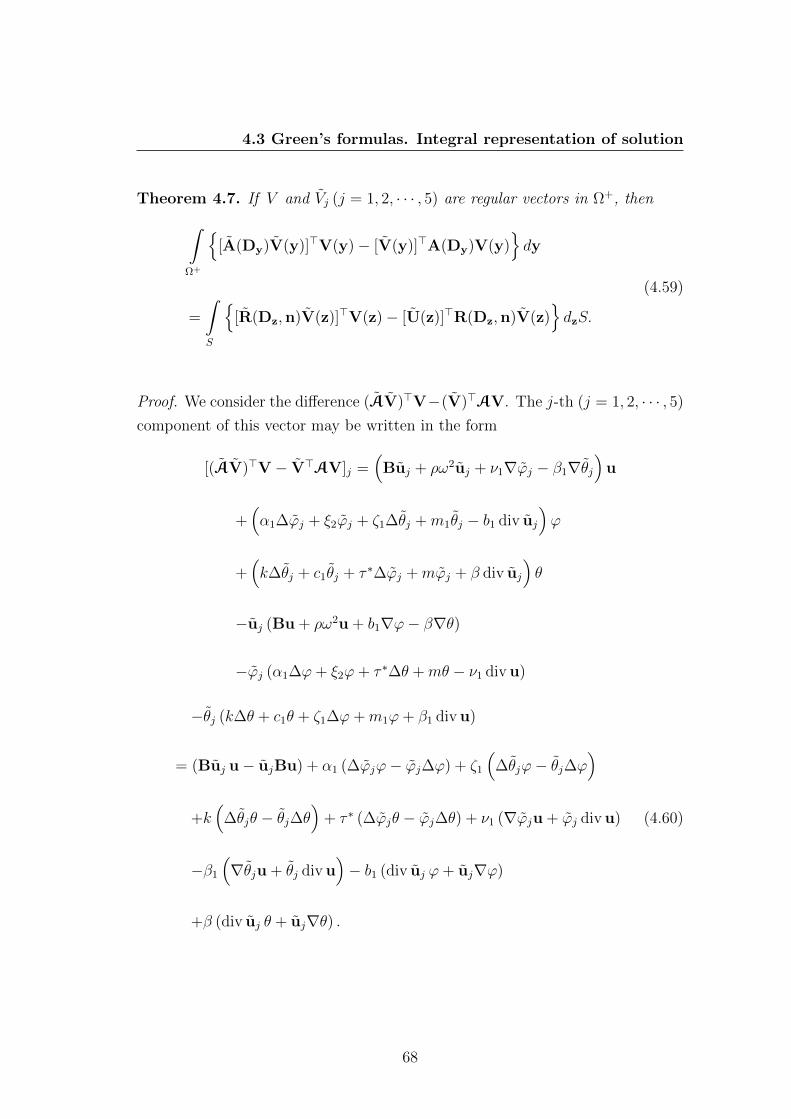
4.3 Green’s formulas. Integral representation of solution
Theorem 4.7. If V and Vj (j = 1, 2, · · · , 5) are regular vectors in Ω+, then∫Ω+
[A(Dy)V(y)]>V(y)− [V(y)]>A(Dy)V(y)
dy
=
∫S
[R(Dz,n)V(z)]>V(z)− [U(z)]>R(Dz,n)V(z)
dzS.
(4.59)
Proof. We consider the difference (AV)>V−(V)>AV. The j-th (j = 1, 2, · · · , 5)
component of this vector may be written in the form
[(AV)>V − V>AV]j =(Buj + ρω2uj + ν1∇ϕj − β1∇θj
)u
+(α1∆ϕj + ξ2ϕj + ζ1∆θj +m1θj − b1 div uj
)ϕ
+(k∆θj + c1θj + τ ∗∆ϕj +mϕj + β div uj
)θ
−uj (Bu + ρω2u + b1∇ϕ− β∇θ)
−ϕj (α1∆ϕ+ ξ2ϕ+ τ ∗∆θ +mθ − ν1 div u)
−θj (k∆θ + c1θ + ζ1∆ϕ+m1ϕ+ β1 div u)
= (Buj u− ujBu) + α1 (∆ϕjϕ− ϕj∆ϕ) + ζ1
(∆θjϕ− θj∆ϕ
)+k(
∆θjθ − θj∆θ)
+ τ ∗ (∆ϕjθ − ϕj∆θ) + ν1 (∇ϕju + ϕj div u)
−β1
(∇θju + θj div u
)− b1 (div uj ϕ+ uj∇ϕ)
+β (div uj θ + uj∇θ) .
(4.60)
68
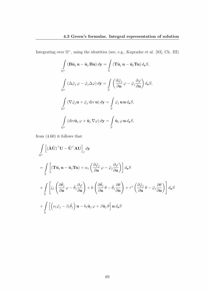
4.3 Green’s formulas. Integral representation of solution
Integrating over Ω+, using the identities (see, e.g., Kupradze et al. [83], Ch. III)∫Ω+
(Buj u− uj Bu) dy =
∫S
(Tuj u− ujTu) dzS,
∫Ω+
(∆ϕj ϕ− ϕj∆ϕ) dy =
∫S
(∂ϕj∂n
ϕ− ϕj∂ϕ
∂n
)dzS,
∫Ω+
(∇ϕju + ϕj div u) dy =
∫S
ϕj u n dzS,
∫Ω+
(divuj ϕ+ uj∇ϕ) dy =
∫S
uj ϕn dzS,
from (4.60) it follows that∫Ω+
[(AU)>U− U>AU
]jdy
=
∫S
[(Tuj u− ujTu) + α1
(∂ϕj∂n
ϕ− ϕj∂ϕ
∂n
)]dzS
+
∫S
[ζ1
(∂θj∂n
ϕ− θj∂ϕ
∂n
)+ k
(∂θj∂n
θ − θj∂θ
∂n
)+ τ ∗
(∂ϕj∂n
θ − ϕj∂θ
∂n
)]dzS
+
∫S
[(ν1ϕj − β1θj
)u− b1uj ϕ+ βuj θ
]n dzS
69
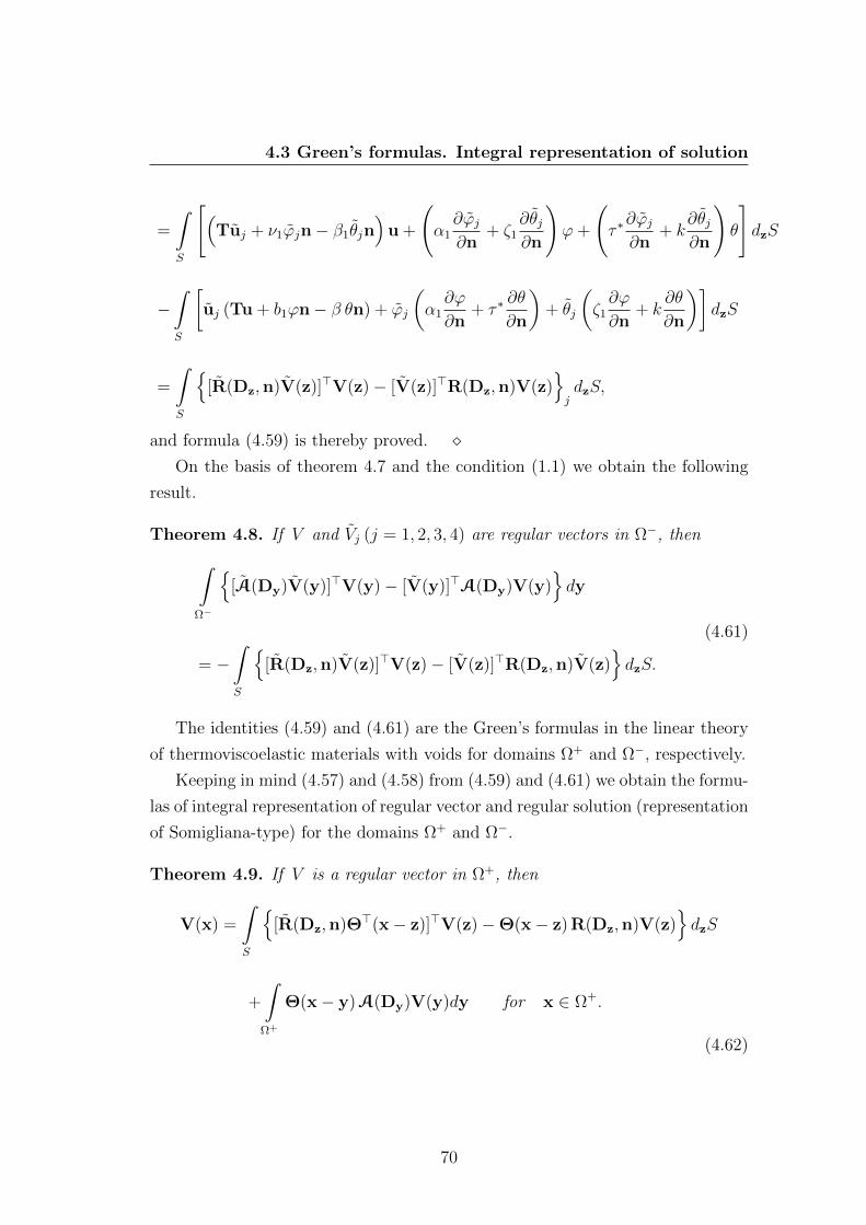
4.3 Green’s formulas. Integral representation of solution
=
∫S
[(Tuj + ν1ϕjn− β1θjn
)u +
(α1∂ϕj∂n
+ ζ1∂θj∂n
)ϕ+
(τ ∗∂ϕj∂n
+ k∂θj∂n
)θ
]dzS
−∫S
[uj (Tu + b1ϕn− β θn) + ϕj
(α1∂ϕ
∂n+ τ ∗
∂θ
∂n
)+ θj
(ζ1∂ϕ
∂n+ k
∂θ
∂n
)]dzS
=
∫S
[R(Dz,n)V(z)]>V(z)− [V(z)]>R(Dz,n)V(z)
jdzS,
and formula (4.59) is thereby proved. On the basis of theorem 4.7 and the condition (1.1) we obtain the following
result.
Theorem 4.8. If V and Vj (j = 1, 2, 3, 4) are regular vectors in Ω−, then∫Ω−
[A(Dy)V(y)]>V(y)− [V(y)]>A(Dy)V(y)
dy
= −∫S
[R(Dz,n)V(z)]>V(z)− [V(z)]>R(Dz,n)V(z)
dzS.
(4.61)
The identities (4.59) and (4.61) are the Green’s formulas in the linear theory
of thermoviscoelastic materials with voids for domains Ω+ and Ω−, respectively.
Keeping in mind (4.57) and (4.58) from (4.59) and (4.61) we obtain the formu-
las of integral representation of regular vector and regular solution (representation
of Somigliana-type) for the domains Ω+ and Ω−.
Theorem 4.9. If V is a regular vector in Ω+, then
V(x) =
∫S
[R(Dz,n)Θ>(x− z)]>V(z)−Θ(x− z) R(Dz,n)V(z)
dzS
+
∫Ω+
Θ(x− y)A(Dy)V(y)dy for x ∈ Ω+.
(4.62)
70
4.3 Green’s formulas. Integral representation of solution
Theorem 4.10. If V is a regular vector in Ω−, then
V(x) = −∫S
[R(Dz,n)Θ>(x− z)]>V(z)−Θ(x− z) R(Dz,n)V(z)
dzS
+
∫Ω−
Θ(x− y)A(Dy)V(y)dy for x ∈ Ω−.
(4.63)
Obviously, on the basis of (4.62) and (4.63) we have the following results.
Corollary 4.3. If V is a regular solution of (4.4) in Ω+, then
V(x) =
∫S
[R(Dz,n)Θ>(x− z)]>V(z)−Θ(x− z) R(Dz,n)V(z)
dzS
for x ∈ Ω+.
Corollary 4.4. If V is a regular solution of (4.4) in Ω−, then
V(x) = −∫S
[R(Dz,n)Θ>(x− z)]>V(z)−Θ(x− z) R(Dz,n)V(z)
dzS
(4.64)
for x ∈ Ω−.
Keeping in mind the conditions (1.1) and (4.10) from (4.64) we obtain
Vj(x) = e−κ0|x|O(|x|−1),
Vj,l(x) = e−κ0|x|O(|x|−1) for |x| 1,
(4.65)
where κ0 = min Imκ1, Imκ2, Imκ3, Imκ4 > 0, l = 1, 2, 3, j = 1, 2, 3, 4.
71
Chapter 5
Boundary value problems in the
theory of thermoviscoelasticity
for materials with voids
5.1 Basic boundary value problems
In the sequel we use the matrix differential operators
1)
R(1)(Dx,n) = (R(1)pq (Dx,n))3×5,
R(1)lj (Dx,n) = µ1δlj
∂
∂n+ µ1nj
∂
∂xl+ λ1nl
∂
∂xj,
R(1)l4 (Dx,n) = b1 nl, R
(1)l5 (Dx,n) = −βnl;
2)
R(2)(Dx,n) = (R(2)pq (Dx,n))1×5, R
(2)1l (Dx,n) = 0,
R(2)14 (Dx,n) = α1
∂
∂n, R
(2)15 (Dx,n) = τ ∗
∂
∂n;
72
5.1 Basic boundary value problems
3)
R(3)(Dx,n) = (R(3)pq (Dx,n))1×5, R
(3)1j (Dx,n) = 0,
R(3)14 (Dx,n) = ζ1
∂
∂n, R
(3)14 (Dx,n) = k
∂
∂n,
where l, j = 1, 2, 3.
Obviously, we can rewrite the matrix differential operator R(Dx,n) (see
(4.55)) in the form
R(Dx,n) = (Rpq(Dx,n))5×5, Rlq(Dx,n) = R(1)lq (Dx,n),
R4q(Dx,n) = R(2)1q (Dx,n), R5q(Dx,n) = R
(3)1q (Dx,n),
where l = 1, 2, 3, q = 1, 2, · · · , 5.The basic internal and external BVPs of steady vibrations in the theory of
thermoviscoelasticity for Kelvin-Voigt materials with voids are formulated as fol-
lows.
Find a regular (classical) solution to system (4.8) for x ∈ Ω+ satisfying the
boundary condition
limΩ+3x→z∈S
V(x) ≡ V(z)+ = f(z) (5.1)
in the Problem (III)+F,f , and
limΩ+3x→z∈S
R(Dx,n(z))V(x) ≡ R(Dz,n(z))V(z)+ = f(z) (5.2)
in the Problem (IV )+F,f , where F and f are the known five-component vector
functions.
Find a regular (classical) solution to system (4.8) for x ∈ Ω− satisfying the
boundary condition
limΩ−3x→z∈S
V(x) ≡ V(z)− = f(z) (5.3)
73
5.2 Uniqueness theorems
in the Problem (III)−F,f , and
limΩ−3x→z∈S
R(Dx,n(z))V(x) ≡ R(Dz,n(z))V(z)− = f(z) (5.4)
in the Problem (IV )−F,f , where F and f are the known five-component vector
functions, and supp F is a finite domain in Ω−.
5.2 Uniqueness theorems
In this section we prove uniqueness of regular solutions of BVPs (K)+F,f and
(K)−F,f , where K = III, IV .
Theorem 5.1. If condition (4.10) is satisfied, then the internal BVP (K)+F,f
admits at most one regular solution, where K = III, IV.
Proof. Suppose that there are two regular solutions of problem (K)+F,f . Then their
difference V corresponds to zero data (F = f = 0), i.e. V is a regular solution
of problem (K)+0,0, i.e. the vector V = (u, ϕ, θ) is a solution of the system of
homogeneous equations (4.6) satisfying the homogeneous boundary condition
U(z)+ = 0 (5.5)
in the case K = III, and
R(Dz,n(z))U(z)+ = 0 (5.6)
in the case K = IV . Obviously, we can rewrite the boundary condition (5.6) in
the form
R(j)(Dz,n(z))V(z)+ = 0, j = 1, 2, 3. (5.7)
On account of (4.6) from Green’s formula of the classical theory of elasticity
74
5.2 Uniqueness theorems
(see Section 3.2)∫Ω+
[B(Dx) u · u +W (u, λ1, µ1)] dx =
∫S
Tu · u dzS
and identities ∫Ω+
(∇ϕ · u + ϕ divu) dx =
∫S
ϕn · u dzS,
∫Ω+
(∇ θ · u + θ divu) dx =
∫S
θn · u dzS,
it follows that∫Ω+
[B(Dx) u + b1∇ϕ− β∇θ + ρω2 |u|2
]· u +W (1)(V)
dx
=
∫S
R(1)(Dz,n)U(z) · u(z) dzS,
(5.8)
where W (u, λ1, µ1) are given by (3.7) and
W (1)(V) = W (u, λ1, µ1)− ρω2 |u|2 + (b1 ϕ− βθ) div u. (5.9)
By virtue of the first equation of (4.6), the boundary condition (5.5) in the
case K = III and (5.7) in the case K = IV , from (5.8) we get∫Ω+
W (1)(V)dx = 0. (5.10)
75
5.2 Uniqueness theorems
On the other hand, on the basis of identities∫Ω+
[∆ϕ ϕ+ |∇ϕ|2
]dx =
∫S
∂ϕ
∂nϕ dzS,
∫Ω+
[∆ θ ϕ+∇θ · ∇ϕ] dx =
∫S
∂θ
∂nϕ dzS,
we have∫Ω+
[(α1 ∆ + ξ2)ϕ+ (τ ∗∆ +m)θ − ν1div u] ϕ+W (2)(U)
dx
=
∫S
R(2)(Dz,n)U(z) ϕ dzS,
(5.11)
where
W (2)(V) = α1 |∇ϕ|2 − ξ2 |ϕ|2 + τ ∗∇θ∇ϕ−mθϕ+ ν1 div u ϕ. (5.12)
On account of the second equation of (4.6), the boundary condition (5.5) in
the case K = III and (5.7) in the case K = IV , from (5.11) we get∫Ω+
W (2)(V)dx = 0. (5.13)
Quite similarly, from third equation of (4.6) and conditions (5.5) and (5.7) it
follows that ∫Ω+
W (3)(V)dx = 0, (5.14)
where
W (3)(V) = k|∇θ|2 − c1 |θ|2 + ζ1∇ϕ∇θ −m1ϕθ − β1 div u θ. (5.15)
76
5.2 Uniqueness theorems
Hence, from (5.10), (5.13) and (5.14) we have∫Ω+
ωT0 Im
[W (1)(V) +W (2)(V)
]− ReW (3)(V)
dx = 0. (5.16)
On the other hand, by virtue of (2.7), (4.5) and the identity
Im (b1 ϕ div u + ν1 div u ϕ) = −ω(b∗ + ν∗) Re(ϕ div u),
from (5.9), (5.12), (5.15) we obtain
Im[W (1)(V) +W (2)(V)
]= −ωW (u, λ∗, µ∗)− ω(b∗ + ν∗) Re(ϕ div u)− βIm(θ divu)
−ωα∗|∇ϕ|2 − ωξ∗|ϕ|2 + τ ∗ Im(∇θ∇ϕ)−m Im(θϕ),
ReW (3)(V) = k|∇θ|2 − ωβT0 Im(θdiv u)− ωζ∗Im(∇θ∇ϕ)− ωmT0Im(θϕ)
and consequently, we get
ωT0 Im[W (1)(V) +W (2)(V)
]− ReW (3)(V)
= −ω2T0 [W (u, λ∗, µ∗) + (b∗ + ν∗) Re(ϕ div u) + ξ∗|ϕ|2]
−[k |∇θ|2 − ω(ζ∗ + τ ∗T0) Im(∇θ∇ϕ) + ω2T0α
∗|∇ϕ|2]
= −ω2T0
[1
3(3λ∗ + 2µ∗) |div u|2 + (b∗ + ν∗) Re(ϕ div u) + ξ∗|ϕ|2
]
−ω2T0µ∗
[1
2
3∑l,j=1; l 6=j
∣∣∣∣∂uj∂xl+∂ul∂xj
∣∣∣∣2 +1
3
3∑l,j=1
∣∣∣∣∂ul∂xl− ∂uj∂xj
∣∣∣∣2]
−[k |∇θ|2 − ω(ζ∗ + τ ∗T0) Im(∇θ∇ϕ) + ω2T0α
∗|∇ϕ|2].
(5.17)
77
5.2 Uniqueness theorems
Obviously, with the help of (4.10) it follows that
1
3(3λ∗ + 2µ∗)|div u|2 − (b∗ + ν∗) Re(ϕ div u) + ξ∗ |ϕ|2 ≥ 0,
k |∇θ|2 − ω(ζ∗ + τ ∗T0) Im(∇θ∇ϕ) + ω2T0α∗|∇ϕ|2 ≥ 0.
From (5.17) we have ωT0 Im[W (1)(V) +W (2)(V)
]− ReW (3)(V) ≤ 0. On the
basis of (5.16) we obtain
ωT0 Im[W (1)(V) +W (2)(V)
]− ReW (3)(V) = 0.
It is easy to verify that the last equation and (5.17) lead to the following relations
1
3(3λ∗ + 2µ∗)|div u|2 − (b∗ + ν∗) Re(ϕ div u) + ξ∗ |ϕ|2 = 0,
1
2
3∑l,j=1; l 6=j
∣∣∣∣∂uj∂xl+∂ul∂xj
∣∣∣∣2 +1
3
3∑l,j=1
∣∣∣∣∂ul∂xl− ∂uj∂xj
∣∣∣∣2 = 0,
k |∇θ|2 − ω(ζ∗ + τ ∗T0) Im(∇θ∇ϕ) + ω2T0α∗|∇ϕ|2 = 0.
(5.18)
On account of inequalities of (4.10) from (5.18) we have
div u(x) = 0,∂uj(x)
∂xl+∂ul(x)
∂xj= 0,
∂ul(x)
∂xl− ∂uj(x)
∂xj= 0, ϕ(x) = 0,
θ(x) = const, l, j = 1, 2, 3
(5.19)
for x ∈ Ω+. On the basis of (5.19) from third equation of system (4.6) it follows
that θ(x) = 0. In view of (4.7) we get W (u, λ1, µ1) = 0. From (5.9) and (5.10)
we obtain u(x) = 0. Thus, V(x) = 0 for x ∈ Ω+.
Lemma 5.1. If V = (u, ϕ, θ) ∈ C2(Ω) is a solution of the system (4.9) for
78
5.2 Uniqueness theorems
x ∈ Ω, then
u(x) =4∑j=1
u(j)(x), ϕ(x) =3∑l=1
ϕ(l)(x), θ(x) =3∑l=1
θ(l)(x), (5.20)
where Ω is an arbitrary domain in R3, u(j), ϕ(l) and θ(l) satisfy the following
equations
(∆ + κ2j)u
(j)(x) = 0, (∆ + κ2l )ϕ
(l)(x) = 0,
(∆ + κ2l )θ
(l)(x) = 0, l = 1, 2, 3, j = 1, 2, 3, 4.
(5.21)
Proof. Applying the operator div to the first equation of (4.6) we have
(µ2∆ + ρω2) div u + b1 ∆ϕ− β∆θ = 0,
(α1 ∆ + ξ2)ϕ+ (τ ∗∆ +m)θ − ν1div u = 0,
(k∆ + c1) θ + (ζ1∆ +m1)ϕ+ β1 div u = 0.
(5.22)
Clearly, from system (5.22) it follows that
Λ1(∆) div u = 0, Λ1(∆)ϕ = 0, Λ1(∆) θ = 0. (5.23)
Now, applying the operator Λ1(∆) to the first equation of (4.6) and using (5.23)
we obtain
Λ1(∆) (∆ + κ24) u = 0. (5.24)
We introduce the notation
u(j) =
[4∏
p=1;p 6=j
(κ2p − κ2
j)−1(∆ + κ2
p)
]u, j = 1, 2, 3, 4,
ϕ(l) =
[3∏
p=1;p6=l
(κ2p − κ2
l )−1(∆ + κ2
p)
]ϕ, l = 1, 2, 3.
(5.25)
79
5.2 Uniqueness theorems
By virtue of (5.23) and (5.24) the relations (5.20) and (5.21) can be easily
obtained from (5.25). Now let us establish the uniqueness of a regular solution of the external BVPs.
Theorem 5.2. If condition (4.10) is satisfied, then the external BVP (K)−F,fadmits at most one regular solution, where K = III, IV.
Proof. Suppose that there are two regular solutions of problem (K)−F,f . Then
their difference V corresponds to zero data (F = f = 0), i.e. V is a regular
solution of the problem (K)−0,0.
Let Ωr be a sphere of sufficiently large radius r so that Ω+ ⊂ Ωr . By virtue
of (4.6) and the homogeneous boundary condition (f = 0), the formula (5.8) for
the domain Ω−r = Ω− ∩ Ωr can be rewritten as∫Ω−r
W (1)(V)dx =
∫Sr
P(1)(Dz,n)V(z) · u(z) dzS, (5.26)
where Sr is the boundary of the sphere Ωr and n(z) is the external (with respect
to Ωr) unit normal vector to Sr at z. From (5.26) we have∫Ω−
W (1)(V) dx = limr→∞
∫Sr
P(1)(Dz,n)V(z) · u(z) dzS. (5.27)
In addition, on account of (4.65) we have
limr→∞
∫Sr
P(1)(Dz,n)V(z) · u(z) dzS = 0.
Hence, from (5.27) we get ∫Ω−
W (1)(V) dx = 0. (5.28)
80
5.4 Basic properties of thermoelastopotentials
On the other hand, by virtue of (4.65) we obtain∫Ω−
W (j)(V) dx = 0, j = 2, 3. (5.29)
Quite similarly, as in theorem 5.1, on the basis of (4.6), (4.10) from (5.28) and
(5.29) it follows that U(x) = 0 for x ∈ Ω−.
Remark 5.1. In Pamplona et al. [103], the uniqueness and analyticity of
solutions of the initial-BVPs in the linear theory of thermoviscoelasticity for
anisotropic Kelvin-Voigt materials with voids are proved.
5.3 Basic properties of thermoelastopotentials
On the basis of Somigliana-type integral representation of regular vector (see,
(4.62) and (4.63)) we introduce the following notations
Z(1)(x,g) =
∫S
Θ(x− y)g(y)dyS,
Z(2)(x,g) =
∫S
[P(Dy,n(y))Θ>(x− y)]>g(y)dyS,
Z(3)(x,φ,Ω±) =
∫Ω±
Θ(x− y)φ(y)dy,
where g and φ are five-component vectors.
As in classical theory of thermoelasticity (see, e.g. Kupradze et al. [83]), the
vector functions Z(1)(x,g), Z(2)(x,g) and Z(3)(x,φ,Ω±) are called single-layer,
double-layer and volume potentials in the linear theory of thermoviscoelasticity
for Kelvin-Voigt materials with voids, respectively.
Obviously, on the basis of (4.62) and (4.63), the regular vector V(x) in Ω+
81
5.4 Basic properties of thermoelastopotentials
and Ω− is represented by sum of the thermoelastopotentials as follows
V(x) = Z(2)(x, V+
)−Z(1)
(x, RV+
)+ Z(3)
(x,AV,Ω+
)for x ∈ Ω+
and
V(x) = −Z(2)(x, V−
)+Z(1)
(x, RV−
)+Z(3)
(x,AV,Ω−
)for x ∈ Ω−,
respectively.
The basic properties of potentials Z(1)(x,g), Z(2)(x,g) and Z(3)(x,φ,Ω±) are
given in the following theorems.
Theorem 5.3. If S ∈ C2,p, g ∈ C1,p ′(S), 0 < p ′ < p ≤ 1, then:
a)
Z(1)(·,g) ∈ C0,p ′(R3) ∩ C2,p ′(Ω±) ∩ C∞(Ω±),
b)
A(Dx)Z(1)(x,g) = 0 for x ∈ Ω±,
c)
R(Dz,n(z))Z(1)(z,g)± = ∓ 1
2g(z) + R(Dz,n(z))Z(1)(z,g) for z ∈ S,
(5.30)
d) R(Dz,n(z))Z(1)(z,g) is a singular integral for z ∈ S.
Theorem 5.4. If S ∈ C2,p, g ∈ C1,p ′(S), 0 < p ′ < p ≤ 1, then:
a)
Z(2)(·,g) ∈ C1,p ′(Ω±) ∩ C∞(Ω±),
b)
A(Dx)Z(2)(x,g) = 0 for x ∈ Ω±,
c)
Z(2)(z,g)± = ± 1
2g(z) + Z(2)(z,g) for z ∈ S, (5.31)
d) Z(2)(z,g) is a singular integral for z ∈ S,
82
5.4 Basic properties of thermoelastopotentials
e)
R(Dz,n(z))Z(2)(z,g)+ = R(Dz,n(z))Z(2)(z,g)− for z ∈ S.
Theorem 5.5. If S ∈ C1,p, φ ∈ C0,p ′(Ω+), 0 < p ′ < p ≤ 1, then:
a)
A(3)(·,φ,Ω+) ∈ C1,p′(R3) ∩ C2(Ω+) ∩ C2,p′(Ω+0 )
b)
A(Dx)Z(3)(x,φ,Ω+) = φ(x) for x ∈ Ω+
where Ω+0 is a domain in R3 and Ω+
0 ⊂ Ω+.
Theorem 5.6. If S ∈ C1,p, suppφ = Ω ⊂ Ω−, φ ∈ C0,p ′(Ω−), 0 < p ′ < p ≤ 1,
then:
a)
Z(3)(·,φ,Ω−) ∈ C1,p′(R3) ∩ C2(Ω−) ∩ C2,p′(Ω−0 ),
b)
A(Dx)Z(3)(x,φ,Ω−) = φ(x) for x ∈ Ω−,
where Ω is a finite domain in R3 and Ω−0 ⊂ Ω−.
Theorems 5.3 to 5.6 can be proved similarly to the corresponding theorems in
the classical theory of thermoelasticity (for details, see Kupradze et al. [83], Ch.
X).
83
5.4 Basic properties of thermoelastopotentials
We introduce the notation
K(5)g(z) ≡ 1
2g(z) + Z(2)(z,g),
K(6)g(z) ≡ −1
2g(z) + P(Dz,n(z))Z(1)(z,g),
K(7)g(z) ≡ −1
2g(z) + Z(2)(z,g),
K(8)g(z) ≡ 1
2g(z) + P(Dz,n(z))Z(1)(z,g),
Kχg(z) ≡ −1
2g(z) + χZ(2)(z,g) for z ∈ S,
(5.32)
where χ is a complex parameter. On the basis of theorems 5.3 and 5.4, K(j) (j =
5, 6, 7, 8) and Kχ are singular integral operators (see Mikhlin [81], Kupradze et
al. [83]).
In the sequel we need the following Lemmas.
Lemma 5.2. If condition (4.10) is satisfied, then the singular integral operators
K(j)(j = 5, 6, 7, 8) are of the normal type.
Proof: Let σ(j) = (σ(j)lm)5×5 be the symbol of the singular integral operator
K(j) (j = 5, 6, 7, 8) (see, Mikhlin [81]). Taking into account (5.32) we find
det σ(j) =
(−1
2
)5 [1− µ2
1
(λ1 + 2µ1)2
]= −(λ1 + µ1)(λ1 + 3µ1)
32(λ1 + 2µ1)2. (5.33)
Keeping in mind the relations (4.10) from (5.33) we have
det σ(j) 6= 0. (5.34)
Hence, the operator K(j) is of the normal type, where j = 5, 6, 7, 8.
Lemma 5.3. If L is a continuous curve on the complex plane connecting the
origin with the point χ0 and Kχ is a normal type operator for any χ ∈ L, then
84
5.5 Existence theorems
the index of the operator Kχ0 vanishes, i.e.
ind Kχ0 = 0.
Lemma 5.3 for an arbitrary singular integral operator is proved in Kupradze
et al. [83], Ch. IV.
Lemma 5.4. If conditions (4.10) are satisfied, then the Fredholm’s theorems
are valid for the singular integral operator K(j) (K(j) is Fredholmian), where
j = 5, 6, 7, 8.
Proof: Let σχ and ind Kχ be the symbol and the index of the operator Kχ,
respectively. It may be easily shown that
det σχ = −(λ1 + 2µ1)2 − µ21χ
2
32(λ1 + 2µ1)2
and det σχ vanishes only at two points χ1 and χ2 of the complex plane. By virtue
of (5.34) and det σ1 = detσ(5) we get χl 6= 1 for l = 1, 2. By Lemma 5.3 we have
indK(5) = ind K1 = 0.
Quite similarly we obtain indK(6) = 0. Obviously, the operators K(7) and
K(8) are the adjoint operators for K(6) and K(5), respectively. Evidently,
indK(7) = −indK(6) = 0, indK(8) = −indK(5) = 0.
Thus, the singular integral operator K(j) (j = 5, 6, 7, 8) is of the normal type
with an index equal to zero. Consequently, the Fredholm’s theorems are valid for
K(j).
5.4 Existence theorems
Obviously, by theorems 5.5 and 5.6 the volume potential Z(3)(x,F,Ω±) is a
regular solution of the system of nonhomogeneous equations (4.8), where F ∈
85
5.5 Existence theorems
C0,p ′(Ω±), 0 < p ′ ≤ 1; supp F is a finite domain in Ω−. Therefore, further we
will consider problem (K)±0,f for K = III, IV.
Now we prove the existence theorems of the regular (classical) solutions of
problems (K)+0,f and (K)−0,f for K = III, IV.
Problem (III)+0,f . We seek a regular solution to internal BVP (III)+
0,f in the
form
V(x) = Z(2)(x,g) for x ∈ Ω+, (5.35)
where g is the required five-component vector function.
By theorem 5.4 the vector function V is a solution of homogeneous equation
(4.9) for x ∈ Ω+. Keeping in mind the boundary condition (5.1), using (5.31) and
(5.32), from (5.35) we obtain, for determining the unknown vector g, a singular
integral equation
K(5)g(z) = f(z) for z ∈ S. (5.36)
By lemma 5.4 the Fredholm’s theorems are valid for operator K(5). We prove that
(5.36) is always solvable for an arbitrary vector f . Let us consider the associate
homogeneous equation
K(8)h0(z) = 0 for z ∈ S, (5.37)
where h0 is the required five-component vector function. Now we prove that
(5.37) has only the trivial solution.
Indeed, let h0 be a solution of the homogeneous equation (5.37). On the basis
of theorem 5.3 and (5.37) the vector function V(x) = Z(1)(x,h0) is a regular so-
lution of the homogeneous BVP (IV )−0,0. Using theorem 5.2, the problem (IV )−0,0
has only the trivial solution, that is
V(x) = 0 for x ∈ Ω−. (5.38)
On the other hand, by theorem 5.3 and (5.38) we get
V(z)+ = V(z)− = 0 for z ∈ S,
86
5.5 Existence theorems
i.e., the vector V(x) is a regular solution of problem (III)+0,0. Using theorem 5.1,
the problem (III)+0,0 has only the trivial solution, that is
V(x) = 0 for x ∈ Ω+. (5.39)
By virtue of (5.38), (5.39) and identity (5.30) we obtain
h0(z) = R(Dz,n)V(z)− − R(Dz,n)V(z)+ = 0 for z ∈ S.
Thus, the homogeneous equation (5.37) has only the trivial solution and therefore
(5.36) is always solvable for an arbitrary vector f .
We have thereby proved
Theorem 5.7. If S ∈ C2,p, f ∈ C1,p ′(S), 0 < p ′ < p ≤ 1, then a regular solution
of problem (III)+0,f exists, is unique and is represented by double-layer potential
(5.35), where g is a solution of the singular integral equation (5.36) which is al-
ways solvable for an arbitrary vector f .
Problem (IV )−0,f . We seek a regular solution to problem (IV )−0,f in the form
V(x) = Z(1)(x,h) for x ∈ Ω−, (5.40)
where h is the required five-component vector function.
Obviously, by theorem 5.3 the vector function V is a solution of (4.9) for
x ∈ Ω−. Keeping in mind the boundary condition (5.4), using (5.30) and (5.32),
from (5.40) we obtain, for determining the unknown vector h, a singular integral
equation
K(8)h(z) = f(z) for z ∈ S. (5.41)
It has been proved above that the corresponding homogeneous equation (5.37)
has only the trivial solution. Hence, it follows that (5.41) is always solvable for
an arbitrary vector f .
We have thereby proved
Theorem 5.8. If S ∈ C2,p, f ∈ C0,p ′(S), 0 < p ′ < p ≤ 1, then a regular solution
87
5.5 Existence theorems
of problem (IV )−0,f exists, is unique and is represented by single-layer potential
(5.40), where h is a solution of the singular integral equation (5.41) which is al-
ways solvable for an arbitrary vector f .
Problem (IV )+0,f . We seek a regular solution to problem (IV )+
0,f in the form
V(x) = Z(1)(x,g) for x ∈ Ω+, (5.42)
where g is the required five-component vector function.
Obviously, by theorem 5.3 the vector function V is a solution of (4.9) for
x ∈ Ω+. Keeping in mind the boundary condition (5.2), using (5.30) and (5.32),
from (5.42) we obtain, for determining the unknown vector g, a singular integral
equation
K(6)g(z) = f(z) for z ∈ S. (5.43)
By lemma 5.4 the Fredholm’s theorems are valid for operator K(6). We prove
that (5.43) is always solvable for an arbitrary vector f . Let us consider the
corresponding homogeneous equation
K(6)g0(z) = 0 for z ∈ S, (5.44)
where g0 is the required five-component vector function. Now we prove that
(5.44) has only the trivial solution.
Indeed, let g0 be a solution of the homogeneous equation (5.44). On the basis
of theorem 5.3 and (5.44) the vector V(x) = Z(1)(x,g0) is a regular solution of
problem (IV )+0,0. Using theorem 5.1, the problem (IV )+
0,0 has only the trivial
solution, i.e., we have the condition (5.39).
On the other hand, by theorem 5.3 and (5.39) we get V(z)− = 0 for z ∈ S.
Hence, the vector V(x) is a regular solution of problem (III)−0,0. On the basis of
theorem 5.2, the problem (III)−0,0 has only the trivial solution, i.e., we obtain the
condition (5.38). By virtue of (5.38), (5.39) and identity (5.30) it follows that
g0(z) = R(Dz,n)V(z)− − R(Dz,n)V(z)+ = 0 for z ∈ S.
88
5.5 Existence theorems
Thus, the homogeneous equation (5.44) has only a trivial solution and therefore
(5.43) is always solvable for an arbitrary vector f .
We have thereby proved
Theorem 5.9. If S ∈ C2,p, f ∈ C0,p ′(S), 0 < p ′ < p ≤ 1, then a regular solution
of problem (IV )+0,f exists, is unique and is represented by single-layer potential
(5.42), where g is a solution of the singular integral equation (5.43) which is al-
ways solvable for an arbitrary vector f .
Problem (III)−0,f . We seek a regular solution to problem (III)−0,f in the form
V(x) = Z(2)(x,h) for x ∈ Ω−, (5.45)
where h is the required five-component vector function.
Obviously, by theorem 5.3 the vector function V is a solution of (4.9) for
x ∈ Ω−. Keeping in mind the boundary condition (5.3), using (5.31) and (5.32),
from (5.45) we obtain, for determining the unknown vector h, a singular integral
equation
K(7)h(z) = f(z) for z ∈ S. (5.46)
It has been proved above that the corresponding associate homogeneous equation
(5.44) has only the trivial solution. Hence, it follows that (5.46) is always solvable
for an arbitrary vector f .
We have thereby proved
Theorem 5.10. If S ∈ C2,p, f ∈ C1,p ′(S), 0 < p ′ < p ≤ 1, then a regular
solution of problem (III)−0,f exists, is unique and is represented by double-layer
potential (5.45), where h is a solution of the singular integral equation (5.46)
which is always solvable for an arbitrary vector f .
Remark 5.2. In Pompei and Scalia [44], the BVPs of steady vibrations in a
linear theory of homogeneous and isotropic thermoelastic solids with voids is
considered. First, integral relations of Betti type are established. The singular
solutions corresponding to concentrated sources are used to derive representations
of Somigliana type. Then, radiation conditions are introduced and a uniqueness
89
5.5 Existence theorems
result for the external problem is established. The potentials of single layer and
double layer are used to reduce the BVPs to singular integral equations for which
Fredholm’s theorems hold. The existence theorems for external problems are
proved.
Remark 5.3. In Pamplona et al. [104], the analyticity of solutions of the initial-
BVPs in the linear theory of thermoviscoelasticity with microtemperatures for
porous materials is proved.
Remark 5.4. Recently, Iesan and Quintanilla [105] presented a strain gradient
theory of thermoviscoelasticity in which the time derivatives of the strain tensors
are included in the set of independent constitutive variables. The basic equations
of the linear theory are derived. The uniqueness and existence theorems in the
considered theory are proved.
90
Chapter 6
Concluding remarks
In this chapter the basis results of the presented thesis are summarized and some
fields of application of there results are analyzed.
In the Chapters 2 to 5 the 3D linear theories of viscoelasticity and thermovis-
coelasticity for Kelvin-Voigt materials with voids are investigated and some basic
results of the classical theories of elasticity and thermoelasticity are generalized.
Indeed:
1. The basic properties of plane harmonic waves in the linear theory of vis-
coelasticity for Kelvin-Voigt materials with voids are established. There are two
(P1 and P2) longitudinal and two (SH and SV ) transverse attenuated plane waves
in the Kelvin-Voigt material with voids;
2. The explicit expressions of fundamental solutions for the systems of equa-
tions of steady vibrations in the linear theories of viscoelasticity and thermo-
viscoelasticity for Kelvin-Voigt materials with voids is constructed by means of
elementary functions. The Green’s formulas in the considered theories are ob-
tained;
3. The representations of Galerkin type solutions of the systems of nonhomo-
geneous equations of steady vibrations in the linear theories of viscoelasticity and
thermoviscoelasticity for Kelvin-Voigt materials with voids are presented and the
completeness of these solutions is established;
4. The formulas of integral representations of Somigliana type of regular vec-
tor and regular (classical) solution are obtained;
91
6. Concluding remarks
5. The representations of general solutions of the systems of homogeneous
equations of steady vibrations in the linear theories of viscoelasticity and ther-
moviscoelasticity for Kelvin-Voigt materials with voids are obtained by using
metaharmonic functions and the completeness of these solutions is established;
6. The basic properties of surface (singe-layer and double-layer) and volume
potentials and singular integral operators are presented. These potentials are
used to reduce the BVPs to singular integral equations for which Fredholm’s the-
orems hold;
7. The uniqueness and existence theorems for classical solutions of the BVPs
of steady vibrations in the linear theories of viscoelasticity and thermoviscoelas-
ticity for Kelvin-Voigt materials with voids are proved by using the potential
method and the theory of singular integral equations.
On the basis of results of this thesis it is possible:
1. To investigate the non-classical problems of the 2D linear theories of vis-
coelasticity and thermoviscoelasticity for Kelvin-Voigt materials with voids;
2. To investigate the non-classical problems in the modern linear theories
of viscoelasticity and thermoviscoelasticity by using potential method and the
theory of singular integral equations for the following materials:
a) a viscoelastic composite as a mixture of a porous elastic solid and a Kelvin-
Voigt material (Iesan [57], Quintanilla [58]),
b) composites modelled as interacting Cosserat continua (Iesan [59]),
c) mixtures where the individual components is modelled as Kelvin-Voigt vis-
coelastic materials (Iesan and Nappa [60]), and
d) Kelvin-Voigt microstretch composite materials (Passarella et al. [66]);
3. To obtain numerical solutions of the BVPs of the linear theory of viscoelas-
ticity for Kelvin-Voigt materials with voids by using of the boundary element
method;
4) To establish basic properties of plane harmonic waves in the linear theories
of viscoelasticity and thermoviscoelasticity for materials with microstructure (see
92
6. Concluding remarks
[58, 59, 60, 66]);
5) To construct the fundamental solutions and to obtain the representations
of general solutions for the systems of governing equations of steady vibrations in
the linear theories of viscoelasticity and thermoviscoelasticity for materials with
microstructure (see [58, 59, 60, 66]);
6) To prove the uniqueness and existence theorems in the modern linear the-
ories of viscoelasticity and thermoviscoelasticity for solids with micro and nanos-
tructures.
93
References
1. Svanadze, M. M.: Steady vibrations problem in the theory of viscoelasticity
for Kelvin-Voigt materials with voids, Proc. Appl. Math. Mech. 12, 283–
284 (2012).
2. Svanadze, M. M.: Potential method in the linear theory of viscoelastic mate-
rials with voids, J. Elasticity 114, 101-126 (2014).
3. Svanadze, M. M.: On the solutions of equations of the linear thermoviscoelas-
ticity theory for Kelvin-Voigt materials with voids, J. Thermal Stresses, 37,
253-269 (2014).
4. Svanadze, M. M.: Potential method in the theory of thermoviscoelasticity for
materials with voids, J. Thermal Stresses, 37, 905-927 (2014).
5. Eringen, A. C.: Mechanics of Continua. R. E. Krieger Publ. Com. Inc, Hunt-
ington, New York (1980), 592 p.
6. Truesdell, C., Noll, W.: The Non-linear Field Theories of Mechanics, 3rd ed.,
Springer-Verlag, Berlin, Haidelberg, New York (2004), 602 p.
7. Christensen, R. M.: Theory of Viscoelasticity, 2nd ed., Dover Publ. Inc., Mi-
neola, New York (2010).
8. Amendola, G., Fabrizio, M., Golden, J. M.: Thermodynamics of Materials
with Memory: Theory and Applications. Springer, New York, Dordrecht,
Heidelberg, London (2012), 572 p.
9. Shaw, M. T., MacKnight, W. J.: Introduction to Polymer Viscoelasticity, 3rd
Ed., John Wiley & Sons, Inc., Hoboken, New Jersey (2005), 316 p.
10. Ferry, J. D.: Viscoelastic Properties of Polymers, 3rd Ed., John Wiley &
Sons, New York, (1980), 672 p.
11. Lakes, R.: Viscoelastic Materials. Cambridge University Press, Cambridge,
94
References
New York, Melbourne (2009), 461 p.
12. Voyiadjis, G. Z., Song, C. R.: The Coupled Theory of Mixtures in Geome-
chanics with Applications. Springer-Verlag, Berlin, Heidelberg (2006), 438 p.
13. Polarz, S., Smarsly, B.: Nanoporous Materials. Nanosci. Nanothech. 2, 581–
612 (2001).
14. Chen, D. L., Yang, P. F., Lai, Y. S.: A review of three-dimensional viscoelastic
models with an application to viscoelasticity characterization using nanoin-
dentation. Microelectr. Reliability 52, 541–558 (2012).
15. Gutierrez-Lemini, D.: Engineering Viscoelasticity. Springer, New York, Hei-
delberg, Dordrecht, London (2014), 353 p.
16. Fabrizio, M., Morro, A.: Mathematical Problems in Linear Viscoelasticity.
SIAM, Philadelphia (1992), 203 p.
17. Di Paola, M., Zingales, M.: Exact mechanical models for fractional viscoelas-
tic material, J. Rheology 56, 983 (2012); http://dx.doi.org/10.1122/1.4717492
(22 pages).
18. Di Paola, M., Pinnola, F. P., Zingales, M.: A discrete mechanical model of
fractional hereditary materials, Meccanica 48, 1573–1586 (2013).
19. Fabrizio, M., Lazzari, B.: On the existence and the asymptotic stability of
solutions for linearly viscoelastic solids, Arch. Ration. Mech. Anal. 116,
139–152 (1991).
20. Appleby, J. A. D., Fabrizio, M., Lazzari, B., Reynolds, D.W.: On exponential
asymptotic stability in linear viscoelasticity. Math. Mod. Meth. Appl. Sci.
16, 1677–1694 (2006).
21. Deseri, L., Fabrizio, M., Golden M.: The concept of a minimal state in
viscoelasticity: new free energies and applications to PDEs, Arch. Ration.
Mech. Anal. 181, 43–96 (2006).
22. Fabrizio, M., Giorgi, C., Morro, A.: Free energies and dissipation properties
for systems with memory, Arch. Ration. Mech. Anal. 125, 341–373 (1994).
23. Del Piero, G., Deseri, L.: Monotonic, completely monotonic and exponential
relaxation functions in linear viscoelasticity. Quart. Appl. Math. 53, 273–
300 (1995).
24. Del Piero, G., Deseri, L.: On the analytic expression of the free energy in
95
References
linear viscoelasticity. J. Elasticity 43, 247–278 (1996).
25. Deseri, L., Gentili, G., Golden, M.J.: An explicit formula for the minimum
free energy in linear viscoelasticity. J. Elasticity 54, 141–185 (1999).
26. Deseri, L., Golden, J. M., The minimum free energy for continuous spectrum
materials, SIAM J. Appl. Math. 67, 869–892 (2007).
27. Graffi, D., Fabrizio, M.: Sulla nozione di stato per materiali viscoelastici di
tipo ”rate”, Atti Acc. Lincei, Rend. Fis. 83, 201–208 (1989).
28. Del Piero G., Deseri L.: On the concepts of state and free energy in linear
viscoelasticity, Arch. Ration. Mech. Anal. 138, 1–35 (1997).
29. Nunziato, J. W., Cowin, S. C.: A non-linear theory of elastic materials with
voids, Arch. Ration. Mech. Anal. 72, 175–201 (1979)
30. Cowin, S. C., Nunziato, J. W.: Linear elastic materials with voids, J. Elas-
ticity 13, 125–147 (1983)
31. Cowin, S. C., Puri, P.: The classical pressure vessel problems for linear elastic
materials with voids, J. Elasticity 13, 157–163 (1983).
32. Puri, P., Cowin, S. C.: Plane waves in linear elastic materials with voids, J.
Elast. 15, 167–178 (1985).
33. Iesan, D.: Some theorems in the theory of elastic materials with voids, J.
Elasticity 15, 215–224 (1985).
34. Chandrasekharaiah, D. S.: A uniqueness theorem in the theory of elastic
materials with voids, J. Elasticity 18, 173–179 (1987).
35. Chandrasekharaiah, D. S., Cowin, S. C.: Unified complete solutions for the
theories of thermoelasticity and poroelasticity. J. Elasticity 21, 121–126
(1989).
36. Scarpetta, E.: On the fundamental solutions in micropolar elasticity with
voids, Acta Mechanica 82, 151–158 (1990).
37. Munoz-Rivera, J. E., Quintanilla, R.: On the time polynomial decay in elastic
solids with voids, J. Math. Anal. Appl. 338, 1296-1309 (2008).
38. Pamplona, P., Munoz-Rivera, J. E., Quintanilla, R.: Stabilization in elastic
solids with voids, J. Math. Anal. Appl. 350, 37–49 (2009).
39. Chirita, S., Ghiba, I. D.: Inhomogeneous plane waves in elastic materials
with voids, Wave Motion 47, 333–342 (2010).
40. Chirita, S., Ghiba, I. D.: Strong ellipticity and progressive waves in elastic
96
References
materials with voids, Proc. R. Soc. A 466, 439–458 (2010).
41. Iesan, D.: A theory of thermoelastic materials with voids, Acta Mech. 60,
67-89 (1986).
42. Scalia, A.: A grade consistent micropolar theory of thermoelastic materials
with voids, ZAMM 72, 133–140 (1990).
43. Ciarletta, M.: A solution of Galerkin type in the theory of thermoelastic
materials with voids, J. Thermal Stresses 14, 409-417 (1991).
44. Pompei, A., Scalia, A.: On the steady vibrations of the thermoelastic porous
materials, Int. J. Solids Struc. 31, 2819–2834 (1994).
45. Chirita, S., Scalia, A.: On the spatial and temporal behavior in linear ther-
moelasticity of materials with voids, J. Thermal Stresses 24, 433–455 (2001).
46. Ciarletta, M., Straughan, B.: Thermo-poroacoustic acceleration waves in
elastic materials with voids, J. Math. Anal. Appl. 333, 142-150 (2007).
47. Singh, B.: Wave propagation in a generalized thermoelastic material with
voids, Appl. Math. Comput. 189, 698–709 (2007).
48. Singh, J., Tomar, S. K.: Plane waves in thermo-elastic material with voids,
Mech. Materials 39, 932–940 (2007).
49. Passarella, F.: Some results in micropolar thermoelasticity, Mech. Res. Com.
23, 349–357 (1996).
50. Lebon, G.: A generalized theory of thermoelasticity, J. Tech. Phys. 23,
37–46 (1982).
51. De Cicco, S., Diaco, M.: A theory of thermoelastic materials with voids
without energy dissipation, J. Thermal Stresses 25, 493–503 (2002).
52. Cowin, S. C.: The viscoelastic behavior of linear elastic materials with voids,
J. Elasticity 15, 185–191 (1985).
53. Ciarletta, M., Scalia, A.: On some theorems in the linear theory of viscoelastic
materials with voids, J. Elasticity 25, 149–158 (1991).
54. Scalia, A.: Shock waves in viscoelastic materials with voids. Wave Motion 9,
125-133 (1994).
55. De Cicco, S., Nappa L.: Singular surfaces in thermoviscoelastic materials
with voids, J. Elasticity 73, 191-210 (2003).
56. Martınez, F., Quintanilla, R.: Existence, uniqueness and asymptotic be-
haviour of solutions to the equations of viscoelasticity with voids, Int. J.
97
References
Solids Struct. 35, 3347–3361 (1998).
57. Iesan, D.: On the theory of viscoelastic mixtures, J. Thermal Stresses 27,
1125–1148 (2004).
58. Quintanilla, R.: Existence and exponential decay in the linear theory of
viscoelastic mixtures, European J. Mech. A/Solids 24, 311–324 (2005).
59. Iesan, D.: A theory of thermoviscoelastic composites modelled as interacting
Cosserat continua, J. Thermal Stresses 30, 1269–1289 (2007).
60. Iesan, D., Nappa, L.: On the theory of viscoelastic mixtures and stability,
Math. Mech. Solids 13, 55–80 (2008).
61. Chirita, S., Gales, C., Ghiba, I.D.: On spatial behavior of the harmonic
vibrations in Kelvin-Voigt materials, J. Elasticity 93, 81–92 (2008).
62. Iesan, D.: On a theory of thermoviscoelastic materials with voids, J. Elasticity
104, 369–384 (2011).
63. Svanadze, M. M.: Boundary value problems of the theory of viscoelasticity
for Kelvin-Voigt materials, Proc. Appl. Math. Mech. 10, 307–308 (2010).
64. Svanadze, M. M.: Boundary value problems of steady vibrations in the theory
of thermoviscoelasticity for Kelvin-Voigt materials, Proc. 9th Int. Congress
on Thermal stresses, TS2011, 5–9 June, 2011, Budapest, Hungary, CD of
Papers and http : //ts2011.mm.bme.hu/kivonatok/Maia%20M.%20Svanadze
TS2011 1294776902.pdf.
65. Svanadze, M. M.: Potential method in the linear theories of viscoelasticity
and thermoviscoelasticity for Kelvin-Voigt materials, Technische Mechanik
32, 554–563 (2012).
66. Passarella, F., Tibullo, V., Zampoli, V.: On microstretch thermoviscoelastic
composite materials, Europ. J. Mechanics, A/Solids 37, 294–303 (2013).
67. Sharma, K., Kumar, P.: Propagation of plane waves and fundamental solution
in thermoviscoelastic medium with voids, J. Thermal Stresses 36, 94–111
(2013).
68. Tomar, S. K., Bhagwan, J., Steeb, H.: Time harmonic waves in a thermo-
viscoelastic material with voids, J. Vibr. Control (2013),
DOI: 10.1177/1077546312470479.
69. de Boer, R.: Theory of Porous Media: Highlights in the historical develop-
ment and current state. Springer, Berlin (2000), 618 p.
98
References
70. Iesan, D.: Thermoelastic Models of Continua. Kluwer, Boston (2004), 298 p.
71. Straughan, B.: Stability and wave motion in porous media, Springer, New
York (2008), 437 p.
72. Straughan, B.: Heat Waves, Springer, New York, Dordrecht, Heidelberg,
London (2011), 318 p.
73. Kellogg, O. D.: Foundations of Potential Theory, Berlin, Springer (1929),
384 p.
74. Gunther, N. M.: Potential Theory and its Applications to Basic Problems of
Mathematical Physics, New York, Ungar Publ Co (1967), 338 p.
75. Hsiao, G. C., Wendland, W. L.: Boundary Integral Equations, Springer-
Verlag, Berlin, Heidelberg (2008), 618 p.
76. Cheng, A. H. D., Cheng, D. T.: Heritage and early history of the boundary
element method, Engng. Anal. Boundary Elem. 29, 268–302 (2005).
77. Fredholm, E. I.: Sur une classe d’equations fonctionnelles, Acta Mathematica
27, 365-390 (1903).
78. Muskhelishvili, N. I.: Singular Integral Equations, Noordhoff, Groningen,
Holland (1958), 447 p.
79. Muskhelishvili, N. I.: Some Basic Problems of the Mathematical Theory of
Elasticity, Springer Science+Business Media, Dordrecht, (1977), 732 p.
80. Vekua, I. N.: Shell Theory: General Methods of Construction, Pitman
Advanced Publishing Program, Boston-London-Melbourne (1985), 287 p.
81. Mikhlin, S. G.: Multidimensional Singular Integrals and Integral Equations.
Pergamon Press, Oxford (1965), 259 p.
82. Kupradze, V. D.: Potential Methods in the Theory of Elasticity. Israel Pro-
gram Sci. Trans., Jerusalem (1965), 340p.
83. Kupradze, V. D., Gegelia, T. G., Basheleishvili, M. O., Burchuladze, T. V.:
Three-Dimensional Problems of the Mathematical Theory of Elasticity and
Thermoelasticity, North-Holland Publ. Comp., Amsterdam, New York,
Oxford (1979), 929 p.
84. Burchuladze, T. V., Gegelia, T. G.: The Development of the Potential
Methods in the Elasticity Theory. Metsniereba, Tbilisi (1985), 228 p. (Rus-
sian).
85. Gegelia, T., Jentsch, L.: Potential methods in continuum mechanics. Geor-
99
References
gian Math. J. 1, 599–640 (1994).
86. Achenbach, J. D.: Wave Propagation in Elastic Solids. North-Holland Publ.
Comp., Amsterdam, Oxford, American Elsevier Publ. Comp., Inc., New York
(1975), 425 p.
87. Hormander, L.: The Analysis of Linear Partial Differential Operators II:
differential operators with constant coefficients. Springer-Verlag: Berlin,
Heidelberg, New York, Tokyo, 1983.
88. Sommerfeld, A.: Die Grensche Funktion der Schwingungsgleichung. Jber.
Deutsch. Math. Verein. 21, 309–353 (1912).
89. Kupradze, V. D.: Sommerfeld principle of radiation. Reports Acad. Sci.
USSR 2, 1–7 (1934) (Russian).
90. Vekua, I. N.: On metaharmonic functions. Proc. Tbilisi Math. Inst. Acad.
Sci. Georgian SSR 12, 105–174 (1943) (Russian).
91. Gurtin, M. E.: The linear theory of elasticity. In: Truesdell, C. (ed): Hand-
buch der Physik, vol VIa/2, Springer-Verlag, Berlin, Heidelberg, New York,
1–296 (1972).
92. Hetnarski, R. B., Ignaczak, J.: Mathematical Theory of Elasticity, Taylor &
Francis, New York, London (2004), 821 p.
93. Nowacki, W.: Thermoelasticity, Pergamon Press, Oxford (2004).
94. Sandru, N.: On some problems of the linear theory of asymmetric elasticity,
Int. J. Engng. Sci. 4, 81–96 (1966).
95. Dragos, L.: Fundamental solutions in micropolar elasticity, Int. J. Engng.
Sci. 22, 265–275 (1984).
96. Wang, M. Z., Xu, B. X., Gao, C. F.: Recent general solutions in linear elas-
ticity and their applications, Appl. Mech. Rev. 61, 030803–1–20 (2008).
97. Galerkin, B.: Contribution a la solution generale du probleme de la theorie
de l’elasticite dans le cas de trois dimensions, C. R. Acad. Sci. Paris 190,
1047–1048 (1930).
98. Iacovache, M.: O extindere a metodei lui Galerkin pentru sistemul ecuatiilor
elasticitatii, Bul. St. Acad. Rep. Pop. Romane, Ser. A 1, 593–596 (1949).
99. Chandrasekharaiah, D. S.: Complete solutions in the theory of elastic mate-
rials with voids -I, Quart. J. Mech. Appl. Math. 40, 401–414 (1987).
100. Chandrasekharaiah, D. S.: Complete solutions in the theory of elastic ma-
100
References
terials with voids -II, Quart. J. Mech. Appl. Math. 42, 41–54 (1989).
101. Knops, R. J., Payne, L. E.: Uniqueness Theorems in Linear Elasticity,
Springer, Berlin, Heidelberg, New York (1971).
102. Pompei, A., Scalia, A.: On the steady vibrations of elastic materials with
voids, J. Elasticity 36, 1–26 (1994).
103. Pamplona, P. X., Munoz-Rivera, J. E., Quintanilla, R.: On uniqueness and
analyticity in thermoviscoelastic solids with voids, J. Appl. Anal. Comput.
1, 251–266 (2011).
104. Pamplona, P. X., Munoz-Rivera, J. E., Quintanilla, R.: Analyticity in
porous-thermoelasticity with microtemperatures, J. Math. Anal. Appl.
394, 645–655 (2012).
105. Iesan, D., Quintanilla, R.: On a strain gradient theory of thermoviscoelas-
ticity, Mech. Res. Commun. 48, 52–58 (2013).
101