システム信頼性におけるモンテ・カルロ法の研究

学位授与機関 東京商船大学学位授与年度 1996URL http://id.nii.ac.jp/1342/00000872/

修 士 塾ロ冊 文

題 目

指導教官 伍

課程名

）ス私儲員枇、窃獅ンノ汐・し磁の撤

藤吉信「三

廻電飛圃4

学籍番号・

ラ年’月31日提出 も

9・1，37

薮務・

頁

eONTENTS

工nセ：roduc七ion － 1

Chapter Z ConventionaZ Methods for Analyses

of Sysセem Reユiabiユi七y 5

Chapter 2 Monte Carlo Methods 7

2．1 Basic Definitions 7 2．2 General Principles 9 2．3 ：Basic Characteristics Of Monte Carlo Methods コ．1

Chapter 3 Random Numbers 13

3．1 General RemaTks 13 3．2 Uniform Random Numbers ’ 14 3．3 Other Random Variables 15

Chapter 4 System Reユiability Evaユuation

with Restricted Sampling Z6

4．1 General Rernarks 一 16

Contents 頁

4．2 ProbZem Statements 20 4．3 Nomenc lature 2 Z 4．4 Crude Monte Carlo Method 22 4．5 Variance－Reduc ing Monte Carlo Methods 24

Chapeer 5 Compa＝ison between erude Monte Carlo Method and New Monte Carlo Method

Using a NumericaZ ExampZe 34

5．1 General Remarks 34 5．2 Examp l e 34 5．3 Results and AnaZyses 41

頁 〆

工NTRODUCT’工ON

With the possible exception of environmental and

computer technology， no other branch of applied science

has developed and broadened so dramatically during thi s 20

years as reliability analysis （1）． 工n the early 19601s the

word reliability was used only in isolated sectors of the

aerospace and weapon industries． 工n the liしerature of the

world’s largest manufacturing industry， the chendcal，

there was no article on reliability until 1966， and only a

few before 1970．

For obvious reasons， the earliest impetu＄ forreliability quantification came from the aircraft

industry． After Wor：Ld War 工， as air tra：Efic and crashes

increased， reliability criteria and necessary safety

levels for aircraft performance emerged． Comparisons

between single and multi－engine aircraft were made from

the points oE view of successfuZ flights， and requirements

in terms of accident rates per hours of flying time were

developed．

工n general terms， reliabilit二y．evaluation is the

application of techniques in the quantification o£ the

Introduction頁 2

reliability of a system． The most widely used techniques

of qUant二ification are analyt二ical including fault tree

analysis， F”］7A （2），’ event t ree analys i s， ETA and failure

modes and effect analysis， Frqi A （Z）． The calculations of

reliability evaluation become increasingly difficult as

the system size increases． Monte Carlo methods are used to

evaluate the reliability of such a system．

Monte Carlo simulation（3） is an alt二ernative to t：he

analytical methods since it is by nature iterative． Monte

Carlo simulation functions by observing random numbers

chosen in such a way that they s imulate the phys ical

randorn processes oE the system being evaluated． The

solution i s inferred by the resultant behavior and

interaction of t二he random numbers．

The sys ternatic development of Monte Carlo s iTnula．t±on

st二arted in eamest in 1944， however， the：re are isolat二ed

re ferences to the usage of undeveloped Monte Carlo

techniques long before this． The nuclear industry was one

of the f irst user of Monte Carlo simulation rnethods（3）．

［Vhey have found extens ive applications in the ti eld of

operational research and nuclear physics， where there are

a variety of problems beyond available resources of

theoret二ical mathemat：ics． They have also been employed

sporadically innumerous other fields of science including

chemi stry ， biology， and medicine．．The large demand of

memory and computer t二ime， which in the past was an

rntroduction 頁 3

obstacle for practical applications in reliability

engineering， i s now being met by the high speed modern

computers and by the ava i lability and abundancy of mini－

and even mi cro－cornputers．

The original appeal of the Monte Carlo method lay in the

observation that one could estimat二e re］．iability

straight forwardly by designing a relatively simple （crude

Monte Carlo） sampling plan that required littleinformation about the system under s tudy． However， i t i s

quickly recognized that using moderately advanced sampling

techniques and exploiting even a modest amount of prior

system information could produce estimates with

considerably smaller sampling error for less eost than

the crude Monte Carlo sampling requires． ln the present

paper， a Monte Carlo method is shown to estimate the

reiiability of a large complex system represented by a

reliability block diagram or by a fault tree． Tl Le Monte

Carlo method i s obtained by applying importance sampling

and variance－reducing techniques． ． Chapter 1 discusses conventional methods for analyses of

system reliabilit二y． A simple example of the apPlication is

described． Chapter 2 deals with following： some basic

definitions Eor analyses oE system reliability， thegenerai principles and basic characteristics of Monte

Carlo methods． Chapter 3 introduces the concept of random

mユmbers and their general remarks showing how to generate

a variety of randorn variables．

Introduction．fi” 一一 rr fi一 4CLr一” ．T一一．T

工n Chapter 4， we present a new Monte Carlo meしhod for

system reliability evaluation by using irnportance sampling

and va：riance－reducing t二echniqUes． 工n orde：r to understand，

the new Monte Carlo method i s described by the Venn

diagram representation． Compared wi th the crude Monte

Carlo method， it i s proven that the new Monte Carlo method

can obtain a respectably small st二andard deviation in the

fina1 ：results． This is t二he main conce：rn in Monte Ca：rlo

work（3）． Chapter 5 illustrates a numerical example by the

re l iability block diagram． The example furthermore

veri£ies the results as shown in Chapter 4， i．e．， the new

Monte Carlo method can reduce a srnall standard deviation

than the crude Monte Carlo．

頁 5隔

CHAPTER 1

Conven’ヒiona＝L Meしhods for

Analysis of System ReZiability

The reliability of a system can usually be Eound by

apPlication of probability しheory and it二s combinatorial

properties （4）． The reliability evaluation i s the

application of techniques in the quantification of the

reliability of a system （5）． The most widely used

techniques oE quantification are analytical． Although

several approximations （1）， such as lower and upper

bounds using the inclusion－exclusion principle， ’Esary

and Pro s chan lower and upper bounds， and lowey and upper

bounds using partial minimal cut and pass sets， have been

proposed， they yield only lower and upper bounds of the

reliability． The usual t二ermwise calculation （cut or Pass

sets） becomes impractical for large systems since the

reliability invoives a large number of terms．

Monte Carlo simulation is an alternative to the

analytical methods since it is by nature iterative．

Examples of t二he application of Monte Carlo

techniques to reliability problems are described in

the literatures （4），

Ch．1 Convent ional Methods頁 6

（6）一（10）． Some of them use the direct sampling techniques，

and oしhers employ more sophisticated apProaches． lthen t二he

di rect sampling techniques are used， a large number of

trials are required to obtain reasonably precise estimates

of the ：reliability． 工f， for example， the exact： system

reliability is O．99999， then 1，000，000 trails would yield

about 10 system failures， whereas 10，000 trail couldresult in no system failure and might lead us to conc lude

that the system is completely reliable． On the average，

we reqUire at least 100，000 t二：rails to have a fai］．ure， and

about 10，000，000 trails are required to produce Monte

Carlo estimates with one significant tigure． （13）

proposed the Monte Carlo method with variance－reducing

techniques （3）． Ethere i s， however， no．guarantee that the

method always reduces the variance．

亘＿エ＿一＿

CHAPTER 2

Mon’ヒe Carlo Methods

2．1 Basic definitions

Monte Carlo simulation includes the chance variat±on

ir血erenし in most二real－life problems， hence the descriptive

narne Monte Carlo． Monte Carlo simulation is alternative to

the analytical methods because of its nature it二erative．

Monte Carlo simulation （11）， as shown in Figure 1，

functions by observing random numbers chosen in such a

way t二hat they simulate the physical random processes of

the system to be evaluated． The solution is inferred by

the resultant behavior and interaction oE the random

numbers．

Monte Carlo methods comprise that branch of experimental

mathematics whi ch concerns with experiments on random

nurubers． Here， the experimental mathematics contrasts with

the theoretical mathematics． Mathernatics is often

elassified as either pure or applied， and the fashions

change as the charact：er of mat二hematics does． A relat：ively

Ch．2 Monte Cario Methods頁 8

recent dichotomy contrasts t：he theoretical mathemat二ics

with the experimental mathematics． These designations are

like those commonly used for theoretical and experimental

physics． The essential difference is that theoreticians

deduce conclusions from post二ulates， whereas

experimentalists infer conclusions from observations．エt

is the difference between deduction and induction．

Prob藍ems

Probabilistic pro㏄sses ←一Unknown ・ ●

曹浮≠獅ttles

Sample extraction 一 Statistics

Fig．1 Monte Carlo rRethods

Ch．2 Monte Carlo Methods頁 9

2．2 General principles

Problems handled by Monte Carlo methods are of t二wo types

called probabilistic or deterrninistic according to

whether or not they are directly concerned with the

behavior and outcome of random processes． 工nしhe case of a

probabilistic problem the s implest Monte Carlo approach

is to observe random numbers， chosen in such a way that

they directly simulate the physical random process of the

original problem， and to infer the desired solution from

t二he behavio：r of these random numbers． One of the main

strengthes of theoretical mathematics is its concern with

abstraction and generaユit二y： one can write down symbolic

exPressions or ：Eormal e（luations which abstract二 しhe essence

oE a problem and reveal its underlying struct二ure．

However， this same strength carries with it an inherent

weakness： the more genera l and forrnal i t s language， the

less is theory ready to provide a numerical solution in a

particular application． The idea behind the Monte Carlo

approach to deterministic problems is to exploit its

strengt：h of t：heoret二ical maしhematics while avoiding its

associated weakness with replacing theory by experiment

whenever the fommer falters． SpeciEically， suppose we have

a detertninistic problem which can be formulated in

theoretical language but can not be solved by theoretical

means． Being detertninistic， this problem has no

Ch．2 Monte Carlo Methods頁 ／0

association with random processes； but， when the theory

has exposed it二s underlying st二ructure， we may perhaps

recognize that this structure or formal expression also

describes sorne apparently unrelated raridom processes， and

hence we can so：Lve the det二ermini stic problem numerically

by Monte Carlo s irnulation of the cencomitant probabilistic

problem．

Probabilistic

Problems

Direct

Reproductio

Monte Carlo Methods

×

xxx

Deterministic

Problems

N lndirect

Conversion

Fig．2 Monte Carlo methods

Ch．2 Monte Cario Methods．夏．＿．．［！

2．3 Basic Characteristics of Monte CarZo methods

Monte Carlo methods， as will be briefly shown lat二er， are

theoretically weZl developed to provide a basis for

analyzing system far more complicated than t二hose to which

analytical or probabilistic methods （12），（13） can apPly，

yet二 it is scarcely used． Monte Carlo simulation can be

used for reliability problems where the system under

investigation is too complex or too large し。 solve

realisしically in any other manner． Electrical power

ロgenerat■on systems represent二 examples of processes where

Monte Carlo tec㎞iques provide the oniy practical

approach to reliability analysis． These systems have large

networks with on一］．ine and standby generaしors at each code．

Inspection of t二he eqUipment may be concu：rrent or on a

st二aggered basis． The sysしem maintenance may be scheduled

or unschedu］．ed， and repair times may vary due to component

types， failure types， and availabi］． ity of repair

personnel． Clearly， any attempt to obtain reliability

parameter for these kinds of problems by deterministic

meしhods is virtually impossible．

Another advanしage of the Monte Carlo techniqUe is the

ease wi th which the number and characteristics of

components may be changed． The crit二ical component s and

fact二〇rs in a system can （luickly be determined by usingしhe

Monte Carlo techni（四e． Most deterministic solutions only

give expected values as results： for examplet expected

Ch．2 Monte Carlo Methods真一＿コ2一＿一＿一

time between failures． Using Monte Carlo methods， a

di stribution of the results can be obtained． The

distribution is usually described as a histogram， but in

most cases， that is sufficient二； nothing rnore is gained by

fitting classic distribution to the results．

Another subtle advantage of the Monte Carlo technique

is that the deve lopment and manipulation oE the Monte

Carlo model provides planing engineers with some

noperating experience” with the system， as well as an

insight into its structure and behavior． Often， that is of

more value than the ouしput二 from a det二ermini stic model，

since the simplifying assumptions’ required to solve a

deterministic model are such that the true complexity of a

large system is seldom understood．

頁 ／3

Chap七er 3

Random Numbers

3．1 General remarks

The essential feature common to all Monte Carlo

computations is t；hat at some points we have t二〇 subsしiしute

for a random variable a corresponding set of actual

values， having t二he stat二istical properties of the random

variable． The values that we substitute are called random

numbers， on the ground that they could we l l have been

produced by chance for a suit二able random process． Thi s

approach mns into in superable practical difficulties

because st二rictly speaking it reqUires us to provide

infinitely many randorn numbers and make intinitely many

statistical tests on them to ensure fully that they meet

the postulates． 工n practice， we produce only finitely many

numbers， subゴect二them to only a few tests， and hope （with

some justificat二ion） that they would have satisfied the

remaining unmade tests． 工n Monte Carlo simulation， using

the random numbers， we can obtain the results whi ch corne

Ch．3 Randorn Numbers 頁 呼

out approximately rights． These random

pseudo－random or quasi－random．

numbers are called

3．2 Uユifor＝n ra二do颯numbers

Monte Carlo simulation includes the change variation

inherent in most real一一life problems， hence the descriptive

name Monte Carlo． The device used to create this variation

when the models are ］un on a digital computer is the

random number generator． Thi s generator usually i s a

subprogram that returns values from a uniforrn di stribution

of the intervals O．O to 1．O． Figure 3 shows a hist二〇gram

constructed from one thousand vaZues generated from RND．

As expected， each of the 10 intervals contains close to

the same number of values． L

100

豊

彗5・

Z

o O．1 O．2 03 O．4 O．5 O．6 Values

Fig．3 Histogram oE values

O．7 O．8

from RND

O．9 1．0

Ch．3 Randorn Numbers頁 ！5

3．3 Other random va＝iables

Algorithrns are available to generate random variables

from distributions by making transformations on one or

several value s generated frorn the uni forrn random number

generator． Binary random variables can be generated as

fOllows： t

Subrouしine binary（P，工） returns one or zero with

probability P or 1－P， respectively． Here， function R］N［D（L）

is used to gene：rate uniform random mユmbers． 工f a uni fo：rm

random number falls in interval（O，P） then value one i s

generated． Otherwise， value zero i s produced．

頁 ／5

Chapter 4

System Reliability Evaluation with Restricted Sampling

4．1 General remarks

Examples of the application oE Monte Carlo techniques to

reliability problems are described in the literature

（4），（6）一（11）． Some of them use the direct sampling

techniques， and the others employ more sophisticqted

apProaches． 工n the direct：sampling cases a large number of

trials are required to obtain reasonably precise estimates

of the reliability．

工n thi s section an improved Monte Carlo method is

developed by applying the importance sampling and

variance－reducingしec㎞iques（3）．工n orderし。 understand，

at first， we use t二he syst：em unavailability to describe the

improved Mont二e Carlo meしhod． We begin by denoting by

rectangle D of Figure 4 as the area from which the direct

Monte Carlo trials are sampled． Assume that the area of D

is unity． Circle s designates the area in which trials

Ch．4 System Reliability Evaluation 夏．，一．エ7．

result in sy＄tem failures． The area of disk s corresponds

to the system unavailability 2s． Note that only a few

trials result in the system・ failures； i’．e． the Venn

diagram representation is not on scale．

Circle S

Rectangle L

Rectangle U

Rectangle D

ロFig．4 Vem diagram representatl．on

Ch．4 System Reliability Evaluation 頁 ／δ

Disk s consists of various system failure modes． Let us

assume now that we can analytically calculate

contribution 2L to system unavailability 2s， 2L which is the

part of the system fiailure modes denoted by rectangle L．

Since the area of rectangle L is 2L， th’e calculation of the

systern unavailability i s reduced to carrying out the

subtraction ［2sr－eL］， which i s repre sented by the shaded area

between circle s and rectangle L． Zn other words， i f M－out

lV trails falユ in the shaded area， t二hen the system

unavailability 2， is

2，＝［2，一 e．］十 2． （4 ．2．O

siE 1）（ll＋2，． （4．2．2）

Similarly， the system reliability Rs is

R，窪好＋R、・ （4・2・3）

Since， part of the system reZiability is calculated

analytically， it can be proven that thi s Mont’e Carlo

estimator has a small variance than the regulqr Monte

Carlo estimator． The technique of subtracting RL is

regarded as an application of a variance－reducing

techmique called the control variate method （3）．

Ch．4 System Reliability Evaluation一一fi－u－uu一一IJgu 一一一一一J一

Let us cons ider now another rectangle， u， which encloses

di sk s． As surne the area u can be calculated analyticaZly

as 2ひ． Let二us restrict the Monte Car］．o trials to the area

between rectangle u and L． In other words， that area is a

universal set． Assume that M－out－of－N Monte Carlo trials

from the area fall on t二he shaded area between circle S and

rectangle L． Then ratio ［2，一2．］／［2．一2．］ is estimated by

！3af，一S？L2L．zl！．一 （4．2．4）

2．一2． N’

Thus， the di f ference ［2s－2L］ i s

2s－2L gi ［2u－2ilבilCl］ （4．2．s）

and the system unavailability 2s i s

2s s；1 ［2u’2L］ב3i｛一＋2L・ （4 ・2・6）

Similarly， the systeni reliab“ity R， is

Rsg［Ru－RL］×l15＋RL・ （4・2・7）’

Since the variance of M／N i s cpmpressed by factor

［Ru－RL］， it can be proven that the Monte Carlo estimator on

the right－hand s ide of （4’．2．7） has smaller variance than

the other one described by （4．2．3）． The following sections

present a formal description of the Monte Carlo method．

Ch．4 System Reliability Evaluation 頁 20

4．2 Problem statement

4．2・1 As sumpt■ons：

：L）．The system has K components， number 1，…ノζ．

2）．Each component is either f㎜ctioning or failed．

3）．States of components are statistically independent．

4）．The system is either furlct二ioning’or failed． The

sysしem is s－coherent．

5）．Some path＆cut sets are㎞own．

ロ4．2．2． NQtat］．on

We

all b，

xi

b

¢（x）

inequality is

O〈 Pr ｛X ＝ b｝ ＝ 1．lll．， Pr〈Xi＝ b i｝ 〈 1’

The prcoblem i s to calculate the

R

assume

the 」

component state

xi＝1， i i component i i‘s £unctioning，

xi＝O， otherwise．

（xi，一・， xk） i s a component state vector．

（b，，…，bk） is a sample vector o£ x．

bi血ary funcしion of フr

ip（x）＝1， iE the system is functioning，

¢（x）＝O， if the system is failed．

sample size．

the reliability o£ the systems

that every state vector is possible， i．e．，

t － t

（4．2．8）

for

system reliability （Z4）

Ch．4 System Reliability Evaiuation 夏＿」≧1

R1Pr ｛¢ （X）＝1｝ （4 ・2・9）

＝2， ip （b） P，｛x＝b｝ （4 ．2．io）

＝．］S¢（X，， … ，J）C，） ”． P，Xt21’一Xt （4．2．11）

＝E． ｛ip （X）〉． （4 ．2．12）

4．3．Nomenclature

Boolea n polynomial： A 2－valued function defining a set

ofi system state vectors； 1 denotes inclusion in the set

and（0差工）noninc lusion．

S－coherent system： A system for which the minimal paths

have only 1－valued e l ernent s and the minimal cuts have only

O－valued elements．

Cornponent： A 2－valued element， where 1 for a success， O

for a faiZure．

Contiguration： A system logic defining which state

vectors are pat二hs， and which are cuts．

Fau：Lt． t：ree： A ：Logica】・ configuration of zero－va］一ued

components， represent ing system failuxe， in an s－coherent

system．

Lattice： A set oE systern－state vector described by a

Boolean Polynomial．

Minimal form： A Boolean polynomial with fewest t二e：rms；

any polynomial wi th the same number of terms has no f ewer

indicator variables．

Ch．4 System Reliability Evaluation 頁 22

Cut： A K－dimensional state vector， representing a

system failure．

Minimal cut： A smallest subset of O－valued components

for system failure； a term of the minirnal form for system

failure， in an s－coherent systera．

Path： A K－dimensional state vector， representing a

system success．

Minima］． path： A smallest subset二〇f］．一valued component：s

Eor system success， in a n s－coherent system； a term of the

minimal form for ¢．

Psuedora ndom variate： A computer－generated uniformly

di s tributed random nuMber between zero and one．

System： A collection of K ？一valued components and their

configuration

Universal set U： The set of 2K state－vectors described

by a Boolean Polynomial．

4．4 Crude Monte Carlo method

Let gs generate ’N statistically independent samples

Ci，一一，CN of x． Figure 5 illustrates the generation of N

samples for component 1． 工n genera1， N×K independent，

dnif。叫rand・m number・are used f・F the generati。n。f N

samples Ci，・一，CN． Each element of sample vector C， can be

obtained by using f㎜ction B工NARY（P，工）of Chapter 3．3． We

evaluate R by the u！［biased binomial estimator Rc （the

subscript c stands ．Eor i’crude”）．

C2tL．2．一SzEgggL1S£ua2i一，3ix一1i“lg131g1iA，ga4StRlabltElt 頁 2う

戎。＝N一・老φ（C，）

工ts variance （15） is

呵箆。｝＝呵N－1煮φ（cル

Us ing the propert±es of expectation and

can obtain the variance．

Var ｛R ．〉 ＝ N一’R （1 一 R）．

Trial no． Random numbers （t）

1

（4．4．1）

（4．4．2）

コvay：Lance， we

（4．4．3）

Blnary value

2

3

1

1

1

N

o．o P，

o．o P，

o．o P，

0．O

コF：L9． 5 Generation oE N sarnples

P，

Eor

1．0

1．0

1 ．0

1．0

component

Cl＝1D

C2＝O

C3＝1

e．＝1

1

Ch．4 System Reliability Evaluation 頁 24・ ｛

4．5Variance－reducing Monte Carlo met：hod

Given a fault tree or a logic diagram for a system with

Kbinary－valued co叩onents， all with㎞own minimal pass

sets Pl，…，Pk， respective工y， we identify a subset of m o：E

the mirlimal paths， calculate the system function assuming

that these are the only minimal paths and define the

binary function as φL． Similarly， let us identify a subset

of the minimal cuしs， calculate the system function by the

only minimal cuts， and define the binary functionφu． The

two binary functions satisfy （4．5．1） and （4．5．2）．

φL（b）≦φ（b）≦φu（b）， for all b （4．5．1）

φL（b）≠0，φゴ（h）≠1． （4．5．2）

We take some， say 配， path sets 1）1，…，P，． of the

statistically cohererlt structure φ． According as it is

shown in Figure 6， we define

φ、（b）§ln【1－lfi bJ． （4・5・3）

j＝1 i∈P／

SupPose that φ五（b）冒1， then， using （4．5．3）， at least one

path seし among 1）1，…，1）m is functioning． Hence φ（b）旨1 resulting

in （4．5．1），（4．5．2） is satisfied by （4．5．3）．

According to Lemma Theorem（15）， the structure function

φ（x）can be simplified by part二ial pivotal decomposition．

Ch．4 Systern ReZiability Evaluation 頁 25

for all x

gb （x） iEE J）c，¢ （1 ，，x） ＋ （1 一xD ¢ （O ．x）

（ご＝1，…ノの． 工t is：

（・ i，」c） ＝ （xl，一一・，xi－1， ’ ，JCi．1，…，X．）

（1 ，，x） i： （x，，‘t・，x，一i， 1 ，xi．i，…，JU．）

（O i，x） i （x ，，…，x，． ，， O ，x，． ，，・・t，x．）．

（4．5．4）

Topevent

G，

B 1．1

Gj

BnLl

Gm

First min path

Fig．6 Minimal path representation of fault trees

Bi．j） k Bni． rp

jth min path

B1．rn） （Bitm

mth min path

Ch．4 System Reliability Evaluation 頁 26

ip（1，，x） and ip（O，，x） are binary functions obtained by setting

the i th indicator variable x， to unity and zero，

respectively． ［the bina］y functions can be pivoted around

other indicator variables until the result二ing binary

functions cons i st from only independent factors．

The function（4．5．3） can be rewritten as

m＊ ip．（b） ＝ ，．．2E7．， L， （b） ＝ h ， （b）． （4 ． s ．s）

Where each argument二 b， appears at most once in each

polynomial L，（b）．

We take some， say n， cut sets k，，…，k． of the statistically

coherent structureφ． According as it二is shown in Figure 7，

let us define

¢dib） ＝一 1， ［i 一 ，n．．．， （i 一b ）］・

Similarly， by using partial pivotal

the function （4．5．6） can be rewritten as

（4．5．6）

decomposition （1）

π掌

φ・（b）＝憲L・（わ）≡編（わ）・ （4・5・7）

For any given i， O s i s k and （b，，…，b，）， let us define

RL， i（わ1，…，わ）§≡ Σ φL（わ）P7〈κ＝わ｝，

b，．1，”．，b，

（4．5．8）

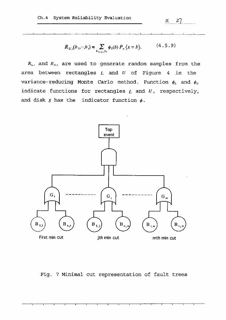
Ch．4 System Reliability Evaluation 夏＿茎7一一一＿

R砿‘（わ1，…，b，）≡ Σ φu（わ）P，｛x＝わ｝．

わご＋1凸b発

（4．5．9）

RL，， and R u， i are used to generate random samples Erorn the

area between rectangles L and U of Figure 4 in the

variance－reducing Monte Carlo method． Funct二ion φL and φσ

indicate functions for rectangles L and U， respectively，

and di sk s has the indicator function ¢．

Topevent

G， Gj Gm

B 1，1 Bni．！

First min cut

B 1，j

jth min cut

Bn，．pa Bi，m Bn，，m

mt．h min cut

Fig． 7 Minirnal cut representation of Eault trees

Ch．4 Systern Reliability Evaluation 耳＿≧δ

RLo and Rσ，o are the reliabilities of the system

represented by φL and φu ， respectively， and are

abbreviated by RL and Rσ respectively． Since RL can never

be higher than the system ：reliability R， as shown in

（16），and 瓦｝ can neve r be lower than i～． The fo］． lowing

ineqμalities hOld

O〈RL≦R≦Rひ＜1． （4．5。10）

工f the e（pUality Rひ＝RL holds， then R＝Rび＝Rゐ and the

problem is trivia1； R can be obtained without the use of

Monte Carlo methods． Therefore let us assume that ’

Ru＞R，． （4．5．ユ1）

This means that rectangle L is included in rect：angle U．

After obtaining t二he reliability functions h乙a：nd hひ， the

funcしions （4．5．8） and （4．5．9） can be ca］．culated．

Rム、（わ、，…，の1h、（わ1，・ψ、，P，｛Xi．1＝1＞，…，P，〈κk＝1｝）

ゴ ・πP・｛Xl＝b，｝ （4・5・1？）

R。，、（わP…，わ、）動。（わ1，…，b、，P，｛κ、．1＝1｝，…，P，｛Xk＝1＞）

ま ・μP，〈Xl＝bi｝ （4・5・・3）

Ch．4 System Reliability Evaluation 頁 zg

Us ing the straight－forward contro l variate method which

is described in the reference （3） to （4．2．10）， the system

reliability can be written．

R＝ “1 7 ［ip （b） 一 ¢L（b）］Pr｛X ： b｝ ＋“F ¢L（b）Pr｛X ＝ b｝ （4 ・5・14）

＝」1 7［¢ （b）一¢L（b）］Pr｛X＝b｝＋RL （4 ・5・15）

［this equation corresponds to （4．2．1）．

For any system－state vector b iE（b，，・一，bD， the structure

function ¢（b）＝1 denotes that b is included ±n the set of

system－success state （17）， （paths）， and ¢（b）＝O membership

in the set of system failure states （cuts）． the terms of

the minimal fo］m of ¢ are the minimal paths， which are

frequently called minimal path sets． For the subset of m

minimal paths and the corresponding lower bound RL， the

structure function ipL（b）＝1 denotes that b i s a mernber of the

set of paths generated by the subset． And ¢L（b）＝O denotes

that b is not a member of that set． On the contrary，

（corresponding to the subset of minimal cuts and the

upper bound R，，）， ¢u（b）＝O denotes that b is in the set of

cuts generated by the subset， and ¢dib）＝1 denotes that b is

not included in the set．

Some of the 2k state vectors in the universal set U are

rlot accounted by either φL or φu．． According to t二he

importance sampling method （3）， let

Ch．4 System Rel±ability Evaluation 頁 30

y謹｛わ：φ。（b）一φ。（わ）＝1｝ （4．5．16）

＝ （PU ¢L

denote the set of st二at二e vectors which are identified

neither as paths under ¢L ， nor as cut s under ipu， and

Xi ｛b： ip （b）一¢．（b）＝1｝ （4 ．5．17）

＝ ip （PL

is the subset of y consisting only of paths．

Using （4．5．11）， and since X E Y， （4．5．15） can be

rewritten as follows：

R＝ ，fF． ［（P （b） 一一 ipL （b）］P．｛x ＝ b｝ ＋ R．

＝【RグR・］、茗，［φ（b）一φ・（わ）齢＝わ｝＋R・ （4・5・・8）

whe re ： y EE （y i， …，y k） E Y i s a random ve c t o r and

P，｛y＝わ｝≡P，｛」C＝わ｝／［RジR」．． （4．5．19）

Since ¢L（b）eO for all b E Y， （4．5．18） becomes：

R ” ［IR u－R“，fF，¢ （b）Pr｛Y ＝ b｝ ＋ RL

Ch．4 System Reliability Evaluation 頁 多ノ

＝［R。一Ril E，〈φω｝＋R，・ （4．5．20）

The variance－reducing Monte Carコ．o method is obtained

from （4．5．20）．

工n the same way as the crude MOnte Carlo method， we

gene：rate N statistically independent sample S1，…，SN of Y． We

ロ

evalugte R by the unbiased binomial est■mator RN as

follOWS：

R”・≡N““”［R・一R」，ヨφ（S，）＋R・・ （4・5・2・）

工tS VarianCe iS

Va・｛i？N｝＝呵N－1脈。一蝋φ（S，）＋碕（4．5．22）

We apPly usefu］． properties of expect二ations （3），so しhat

（4．5．22） can be rewritten to the form

Var〈12．｝＝Var｛N一’［R・．一R躇φ（S ，）〉’（4・5・23）

（4．5．23）is the variance of the arit㎞etical卑ean ofNli．i．d． samples。f［R。一R」φω．且ence

Ch．4 System Reliability Evaluation 亘．．．3≧＿＿＿一

Var｛RA ．｝ ＝N一’ Var｛ ［R ．一Ril¢ （y）｝ （4 ．5．24）

＝ IV 一’E ，｛ ［R ．一R，］ 2ip 2 （y）｝

一’ AI－i｛E，［R ．’R“ip （y）｝ 2． （4 ・5・25）

Since the value of ip（b） is either O or 1， the identity

¢2 （b）s¢（b）． （4 ．5・26）

Us ing （4．5．20） and （4．5．26）， we receive

E，｛（R u－Ri） ¢（Y）｝ ＝R一 RL （4 ．5．27）

E，｛（R ．一 RD 2 ¢2（y）｝ ＝ （R u－RD E，｛（R u ’一 RD ¢（Y）｝

＝ （R．一RD （R 一RD． （4 ．5．28）

工f we use （4．5．27） and （4．5．28） fo：r calcuユation into

（4．5．25）， we can obtain its variance．

Var｛ji？N｝＝N－1（Rひ一R）（R－RD． （4．5．29）

The difference of variance between crude Monte Carlo

method and the variance－reducing Monte Carlo method i s as

follows：

Ch．4 System Rel±ability Evaluation 頁 33

Var｛R ．〉 一 Var｛R ．｝＝ N－i［R （1 一R ．） ＋ R，（R ．一 R）］ 〉 O・（4．5．30）

ThereEore

Var｛乱｝＜Var〈」吏。｝． （4．5．31）

According to definitions（3）， the mean is a measure of

コ のlocation of a random variable， whereas the var■ance エs a

measure oE di spersion about that mean． The standard

deviation is defined by （variance）’h．

The main puηpose in the work with Monte Carlo methods is

to obtain a respecta上）1y small standard deviation in the

fina］． result． In thi s paper， using importance sampling and

variance－reducing tec㎞i（Xues， the standa：ごd deviation is

reduced in t二he fina］． estimator． Moreove：r， Bias a：re pot

introduced into the estimation／ and thus the

variance－reducing Monte Carユ。 makes resu：Lts more precise

without sacrificing reliability．

頁 54

Chapter 5

Comparison between Crude MonteCarlo and New Monte Carlo MethodsUsing A NumeTicaZ ExampZe

5．1． General remarks

1n the previous Chapters， the principles and natures of

Monte Carlo methods are described． Tn the Chapter 4， us±ng

±mportant sample and variance－reducing techniques，

compared wi th the crude Monte Carlo method， a respectabZy

small variance is obtained in the final estimator． We also

use a nurnerical example to evaluate whether or not the

variance－reducing Mont e Carlo method can reduce the

varlance．

5．2 Example

The bridge system is represented by the reliabiZity

block diagram as shown in Figure 8． The reliab±lity of the

component s are P．〈x，＝ 1｝ ＝ ．9 for i＝ 1， … ，5 ．

Ch．5 A Numerical Example 耳一一35＿一一

N ？

5

3 隊

Fig．8 Reliability Block Diagrarn of an Example

The minimal path sets are：

P，＝｛1，2｝

P， ＝ ｛3， 4｝

P， ＝ ｛1， 4， 5｝

P， ＝ ｛2， 3， 5｝．

Ch．5 A Numerical Example

The minimal cut sets are：

K1＝｛1，3｝

κ2＝〈2，4｝

K3＝｛1，4，5｝

K4＝｛2，3，5｝．

We take the pass sets （m＝2）

1）1＝｛1，2＞

P、＝｛3，4＞

and the cut sets （n＝2）

K1＝｛1，3｝

K2＝〈2，4｝．

According to the ident ity，

ア φ（b）≡1一μ［1－P・（わ）］

ア ≡1一据［1一、｛．， b・】

頁 35

（5．1）

Ch．5 A Numerical Example 頁 37

alower bound structure f㎜ctionφLψ）can be written as

follows：

φ。（b）＝1一（1一わ1り（1一わ3わ4）

＝わ1わ2→騨わ3わ4一わ1わ2わ3わ4＝h．（b）． （5．2）

Similarly， the identity

た φψ）…1， Ki（b）・ （5・3）

An upPer bound structure fmctignφひ（b）is：

φσψ）＝［1一（1一わ1）（1一わ，）］［1一（1一り（1一わ、）】

＝わ1わ2＋わ2∂3＋わ1わ4＋わ3わ4＋わ1わ2わ3わ4

一わ1わ2わべわ、わ，ゐ、一わ1わ、わ，一わ1わ，わ．4．

＝hσ（b）． （5．4）

The subsets r and X a：re：

y＝〈わ：φ〆わ）一φ、（b）＝1｝ （5．5）

X＝〈わ：φψ）一φ、（b）＝1｝． （5．6）

Ch．5 A Numerical Example 頁 38

For each component，we can determine whether it is

deterministically l or deterministically O according to Y．

If whichever value is relevant， the subset of stat：e

vect二〇rs with the complementary va lue for which component

is automatically deleted． For those components ／ that are

free to assume eit二her va：Lue， a l is assigned with

probability 1）ノand a O with probability Pノ ． t－

For each random state vector Sγ， γ＝1，…，N which is

generated，φ（Sγ）＝1 denotes that SY is in X， andφ（Sr）ニO

den。tes n・nmembership in X・The fracti・n恩φ（S，）／N den。tes

the estimated proportion of the probability of Y accounted

by X、 weighed by the di fference Rv－RL． The result is added

to RL to yield the statistical：Ly ur丘）iased binomial

ロ ム

estユmator RN：

＾ ム「

R・＝N”1（RゴR∂惹φ（S・）＋R・ （5・7）

The algorithm for generat二ing stat二e vectors S y for the

Monte Carlo trials obtains only elements of y， by

assigning binary component values in order， and one by one

and simultaneously eliminating candidates not in Y． ：Let

b＝（b、，…b，，…，外）denotes a耳y state vector， wit二h the first i－1

componentS b，，…，b、一1 all Specified， the value of b i to be

determined， and the remaining 〃一i component s b，．1，…，b， all

unspeci：Eied．

Ch．5 A Numerical Example 頁 37

Some value are obtained dete］rmini stically．

P．｛b ，｝＝1， if （b i， ”’ bp ”’）EY ， （b i， ”’Si， ”’）eY；

P．｛b ，｝＝O ， if （b ，， …b，， …）¢Y．

And the others are obt二ained by the Monte Carlo method．

P，｛b ，＝ O｝ ＝ 1 一p，， if （b ，， tt・ ，b， 一・一） E Y， （b ，， ・tt S ，， …） G Y；

P，｛b，＝ 1｝ ＝p，， if （b ，， … ，b，・i一）EY， （b ，， ・・tb，， …）EY．

From （4．5．12） and （4．5．13）

RL＝PiP2十PfP，一P，P，P，P， （5．8）

Ru＝PiP2＋P2P3＋P3P4＋PiP4＋PiP2P3P4

－PiP2P4MP2PfP4－PiP2P3－PiP3P4・ （5．9）

The l owe r bound R． and upper bound R u are：

R， ＝O． 964 （s．10）

R． ＝O．980． （5．11）

Ch．5 A NumericaZ Example一fi一．一 ．一 rr ”一． 4一 q一 ．．mJ一 一

The results are clearer in temms of the system

probability． From （5，8） and （5，9）， we obtain

failure

1－R，＝36×10－3 （s．12）

1一一 R．＝ 20×10 ’3． （s．13）

The inequality of （4．5．10） ensures that the system

Eailure probability 1－R lies in the internal［ 20 × 10 一3， 36 × IQ 一3］ ．

The reliability R i s the sum of 25＝32 terms． The minimal

pass sets give the exact system relial）ility R which is

R ＝ O．978 （5．14）

［lie exact system failure probability is

1－R＝ 22 × lo－3 （5．15）

From ．（4．4．5） and （4．529）， we know that the estimators

Rc and RN

deviations：

with N＝2000

UR．＝ 33・1 × 10’‘

UR．＝ 1 × lo－4．

have the following s tandard

（5．16）

（5．17）

Ch．5 A Numerical Exarnple 夏＿41．＿＿

5．3 Resu：Lセs and analyses

ヘ パ

The esしimator．Rc and RN with N are shown in Table 1．

From the Table 1， it is very clear that the standard コロ コ ム ロ ロ

devユ．atユon of RN ：L s much lower than the standard dev■atユon

of 爺。 ， and also much lower thar1 16×10－3， which is the

Zengt4。f intemal【20・10－3・36・10曽3】。f the system failure

probability．

This certifies that the variance－reducing Monte Carlo

method can reduce ▽ariance in the fina］． estimator without

sacrificing reliability．

Ch．5 A Numerical Exarnple 頁 42

Trial

獅浮高b??i

Crude MonteCarIo New Monte Carlo

ARc VarV2o良。｝・10－4 ARN Varv2o食。｝・10”4

100 0，980 145．3 0，978 4．90

200 0，980 102．5 0，978 3．46

300 0，980 83．7 0，978 2．83

400 0，980 72．8 0，978 2．45

500 0，980 64．8 0，978 2．34

600 0，980 59．2 0，978 2．20

700 0，980 54．8 0，978 t73

800 0，980 51．0 0，978 t73

900 0，980 47．9 0，978 1．73

1000 0，980 45．8 0，978 1．41

1200 0，980 42．4 0，978 t41

1500 0，979 37．4 0，978 1．41

1800 0，979 34．6 0，978 1．00

2000 0，979 33」 O，978 tOO

2500 0，979 28．3 0，978 1．00

3000 0，979 26．5 0，978 tOO

3500 0，979 24．5 0，978 1．00

4000 0，979 22．4 0，978 ．tOO

5000 0，979 20．0 0，978 0．00

Table 1． Results of two kinds of Monte CarZo method

．’

Dfi一一”L－T4．TsT 7一一rrnt T

ConcZusion

This pape：r presents』a new ，Monte Carユ。 method for

）stimating the reliability o’ ?large complex systemrepresented by bracketing it between determin±stic lower a nd

rpper bounds， and then positioning R between the bounds as a

ie ighed average of the s txucture function． ［［Wo binary

iunctions are introduced； one dominates the system structure

iunction and the other i s dominated by the structure

iunction． These functions can be constnユcted easily by using

）art of path s ets and cut sets of the sys tem． Tlirough the

Lse of these binary funetions， two variance－reducing

；echniques （controZ variate and import－ance sampZing） are

Lpplied to the Monte Carlo evaluation of the system

reliability．

［ilhe new Monte Carlo method includes following two phases：

1． subset selection． Through using part of minimal path

；ets and cut sets， the reliability R is bracketed between

；he bound R L and R u．

2． Monte Carlo s imulation． By ．applying importance

；ampling and variance－reducing techniques， a reiiability

）stimate with a small variance is obtained．

Conclusion 頁44・

3． Monte Carlo s imulation． By applying ±mportance

sampling and variance－reducing techmiques， a reliability

est二imate wit二h a small variance is obtained．

The procedures is illustrated with a bridge system

represented by the reliability block diagram． 工t is proved

that the new Monte Carlo method gives a reliability

estirnate with a small variance than that of the crude

Monte Carlo method．

With new Monte Carlo method， there are still some

difficulties in using the method． The new Monte Carlo

method cannot be programmed easily as a general pu］fpose

（GP） program． Therefore， we need more theoretical work to

develop an efficient GP prograrn in the next stage．

Acknowledgement

The present auther wishe s to express her s incere thanks

for the consistent guidance given by Professor Y． Sato．

Her thanks are also due for the correction of the English

manuscript carried out by Dr T． 工shimori and for the

research staffs！ assistance． The auther wishes to thank

Association of 工nternational Education， Japan because they

provide her with the scholarship．

頁 4．5’

REFERENCES

1． Ernest 」． Henley， Hiromitsu Kurnamoto， Probabilistic

Risk Assessment， The 工nstitute of E：Lectrical and

Electronics Engineers 工nc．， New York， 199］．．

2． 」． B． Fussel， A Formal Methodology for Fault Tree

Construction， Nuclear Science and Engineers 52， 1973．

3． 」． M． Hammers ley， D． C． Handscomb， Monte Carlo

Me thods， Methuen and Co． Ltd．， London， 1967．

4． Satish J． Kamat， Michael W Ri Zey， Determination of

Relia：bility Using Event－Based Monte Carlo Simulation， 工EEE

Trans． Reliability， vol． R－24， no． 1， Apr． 1975， pp 73－75．

5． A． M． Featherstone， the Application of Monte CarZo

Computer Simulation Techniques Relia：biZity Assessment，

University of Aston， Birmingham， 1986．

6． Satish J． Kamat， William E． Franzmeir， Determination

of Reliability Event－Based Monte Carlo Simulation Part 2，

：EEE Trans． Reliability， vol R－25， Oct． 1976， pp 254－255．

7． P．． W． Becker， Finding the Better of TWo SimUar

Designs by Monte Car］．o Tec㎞iques， 工EEE Trans．

Rel±ability， vol． R－23， Oct． 1974， pp 242－246．

8． M． Mazumbar， 工mporta nce Sa㎎）ling in Reliabi：L ity

Estimation， Reliability and Fault Tree Analysis， SrAM，

1975．

9． Van． Slyke， R． H． Frank， Network Reliability Anaiysis

Part 1， Networks， vol 1， 1972．

Reference

一一g－N．．r“一tt．IP61一一LJ一一一．一．rr

10． Van． S lyke R．， H． Frank， A． Kershenbaum， Network

Reliability AnaZysis Part 2， Reliability and Fault Tree

Analys i s， S工AM， 1975．

li．近藤 次郎，応用確率論，日刊技連，1978

12． M． C． Easton， C． K． Wong， Sequential Destruction

Reliabilityt 工EEE Trans． Reliability， vol R－29， Apr． 1980，

pp 27－32．

13． A． GoZdfeid， A Dubi， Monte Carlo Methods in

Reliability工nternational，σo㎞Wiley 一＆Sons， ししd．， vol 3，

1987．

14． Himomi t su Kumamoし。， ：Ka zuo Tanaka， ：Ko i chi 工noue，

Efficient Evaluation of Syst二em Re：Liability by Monte Carlo

Method， IEEE Trans． ReZiability， vol R－26， Dec． 1977， pp

311 一一315．

15． Richard E． BarZow， Frank Proschan， Statistical

Theory of Reliability and Life Testing ProbabiUity

Mode l s、 Holt， Reinhart and Wins ton 工nc．， 1975．

16． M． O． Lock， the Maximum Error in System Reliability

Ca：Lcu］，ations by Using a Subset of the Minima：L States， 工EEE

Trans． Reliability， vol R－20， Nov． 1971， pp 231－234．

17． Evaiuating the ］M71 Monte Carlo Method for System

Reliability Calculation， IEEE ［rrans． Reliability vol R－28，

No． 5， Dec． Z 979， pp 368－372．

18．森口 繁一，FOR㎜，東京大学出版会，1984

19． Koelbel Charles H， the High Performance Fortran Hand

book Scientific and Engineering Computation， Cambridge，

1994．