
Comparison of Regularization Methods for Feynman Diagrams ...
feynMF:
Drawing Feynman Diagrams
with LATEX and METAFONT∗
Thorsten Ohl†
Technische Hochschule DarmstadtSchloßgartenstr. 9
D-64289 DarmstadtGermany
December 30, 1997
Abstract
feynMF is a LATEX package for easy drawing of professional qualityFeynman diagrams with METAFONT (or META O T). feynMF lays outmost diagrams satisfactorily from the structure of the graph without anyneed for manual intervention. Nevertheless all the power of METAFONT
(or META O T) is available for obscure cases.
Copying
feynMF is free software; you can redistribute it and/or modify it under theterms of the GNU General Public License as published by the Free SoftwareFoundation; either version 2, or (at your option) any later version.feynMF is distributed in the hope that it will be useful, but without any war-ranty; without even the implied warranty of merchantability or fitness for aparticular purpose. See the GNU General Public License for more details.You should have received a copy of the GNU General Public License along withthis program; if not, write to the Free Software Foundation, Inc., 675 Mass Ave,Cambridge, MA 02139, USA.
∗This is feynmf.dtx, version v1.08, revision 1.30, date 1996/12/02.†e-mail: [email protected]
1
Contents
1 Introduction 41.1 Purpose and scope . . . . . . . . . . . . . . . . . . . . . . . . . . 41.2 Relation to similar packages . . . . . . . . . . . . . . . . . . . . . 51.3 Historical note . . . . . . . . . . . . . . . . . . . . . . . . . . . . 61.4 Architecture . . . . . . . . . . . . . . . . . . . . . . . . . . . . . . 61.5 Conclusion . . . . . . . . . . . . . . . . . . . . . . . . . . . . . . 6
2 Usage 82.1 LATEX package and environments . . . . . . . . . . . . . . . . . . 82.2 Auxiliary files . . . . . . . . . . . . . . . . . . . . . . . . . . . . . 92.3 Running METAFONT . . . . . . . . . . . . . . . . . . . . . . . . . 102.4 The feynmf perl script . . . . . . . . . . . . . . . . . . . . . . . . 122.5 Vertex mode . . . . . . . . . . . . . . . . . . . . . . . . . . . . . 13
2.5.1 External vertices . . . . . . . . . . . . . . . . . . . . . . . 142.5.2 Arcs and internal vertices . . . . . . . . . . . . . . . . . . 142.5.3 Polygons . . . . . . . . . . . . . . . . . . . . . . . . . . . 182.5.4 Color . . . . . . . . . . . . . . . . . . . . . . . . . . . . . 192.5.5 Examples . . . . . . . . . . . . . . . . . . . . . . . . . . . 192.5.6 Labels . . . . . . . . . . . . . . . . . . . . . . . . . . . . . 232.5.7 Manipulating the layout . . . . . . . . . . . . . . . . . . . 242.5.8 Skeletons . . . . . . . . . . . . . . . . . . . . . . . . . . . 252.5.9 Pulling strings . . . . . . . . . . . . . . . . . . . . . . . . 27
2.6 Miscellaneous commands . . . . . . . . . . . . . . . . . . . . . . . 292.6.1 Graphs in graphs . . . . . . . . . . . . . . . . . . . . . . . 292.6.2 Reusing diagrams . . . . . . . . . . . . . . . . . . . . . . . 302.6.3 Grouping . . . . . . . . . . . . . . . . . . . . . . . . . . . 302.6.4 Changing parameters . . . . . . . . . . . . . . . . . . . . 312.6.5 Shrinking . . . . . . . . . . . . . . . . . . . . . . . . . . . 312.6.6 Debugging . . . . . . . . . . . . . . . . . . . . . . . . . . . 312.6.7 Multiple vertices and arcs . . . . . . . . . . . . . . . . . . 31
2.7 Immediate mode . . . . . . . . . . . . . . . . . . . . . . . . . . . 322.7.1 Arcs . . . . . . . . . . . . . . . . . . . . . . . . . . . . . . 332.7.2 Vertices . . . . . . . . . . . . . . . . . . . . . . . . . . . . 332.7.3 Declarations . . . . . . . . . . . . . . . . . . . . . . . . . . 332.7.4 Assignments . . . . . . . . . . . . . . . . . . . . . . . . . 342.7.5 Examples . . . . . . . . . . . . . . . . . . . . . . . . . . . 34
2.8 Raw METAFONT . . . . . . . . . . . . . . . . . . . . . . . . . . . 352.8.1 Extending feynMF . . . . . . . . . . . . . . . . . . . . . . 36
2.9 Common traps, trouble shooting and frequently asked questions(FAQs) . . . . . . . . . . . . . . . . . . . . . . . . . . . . . . . . 392.9.1 ! Value is too large . . . . . . . . . . . . . . . . . . 392.9.2 Diagrams in the document are never updated . . . . . . . 402.9.3 Disgrams show up in the wrong spot . . . . . . . . . . . . 402.9.4 Spurious labels show up . . . . . . . . . . . . . . . . . . . 40
2.10 Known bugs . . . . . . . . . . . . . . . . . . . . . . . . . . . . . . 412.10.1 Chaotic manual . . . . . . . . . . . . . . . . . . . . . . . . 412.10.2 Delayed error messages . . . . . . . . . . . . . . . . . . . 412.10.3 Multiple tadpoles . . . . . . . . . . . . . . . . . . . . . . . 41
2

2.10.4 Hard limits . . . . . . . . . . . . . . . . . . . . . . . . . . 41
3
1 Introduction
1.1 Purpose and scope
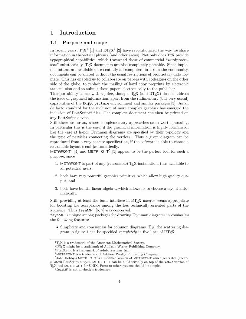
In recent years, TEX1 [1] and LATEX2 [2] have revolutionized the way we shareinformation in theoretical physics (and other areas). Not only does TEX providetypographical capabilities, which transcend those of commercial “wordproces-sors” substantially, TEX documents are also completely portable. Since imple-mentations are available on essentially all computers in use in the community,documents can be shared without the usual restrictions of proprietary data for-mats. This has enabled us to collaborate on papers with colleagues on the otherside of the globe, to replace the mailing of hard copy preprints by electronictransmission and to submit these papers electronically to the publisher.This portability comes with a price, though. TEX (and LATEX) do not addressthe issue of graphical information, apart from the rudimentary (but very useful)capabilities of the LATEX picture environment and similar packages [3]. As ande facto standard for the inclusion of more complex graphics has emerged theinclusion of PostScript3 files. The complete document can then be printed onany PostScript device.Still there are areas, where complementary approaches seem worth pursuing.In particular this is the case, if the graphical information is highly formalized,like the case at hand. Feynman diagrams are specified by their topology andthe type of particles connecting the vertices. Thus a given diagram can bereproduced from a very concise specification, if the software is able to choose areasonable layout (semi-)automatically.METAFONT
4 [4] and META O T5 [5] appear to be the perfect tool for such a
purpose, since
1. METAFONT is part of any (reasonable) TEX installation, thus available toall potential users,
2. both have very powerful graphics primitivs, which allow high quality out-put, and
3. both have builtin linear algebra, which allows us to choose a layout auto-matically.
Still, providing at least the basic interface in LATEX macros seems appropriatefor boosting the acceptance among the less technically oriented parts of theaudience. Thus feynMF
6 [6, 7] was conceived.feynMF is unique among packages for drawing Feynman diagrams in combiningthe following features:
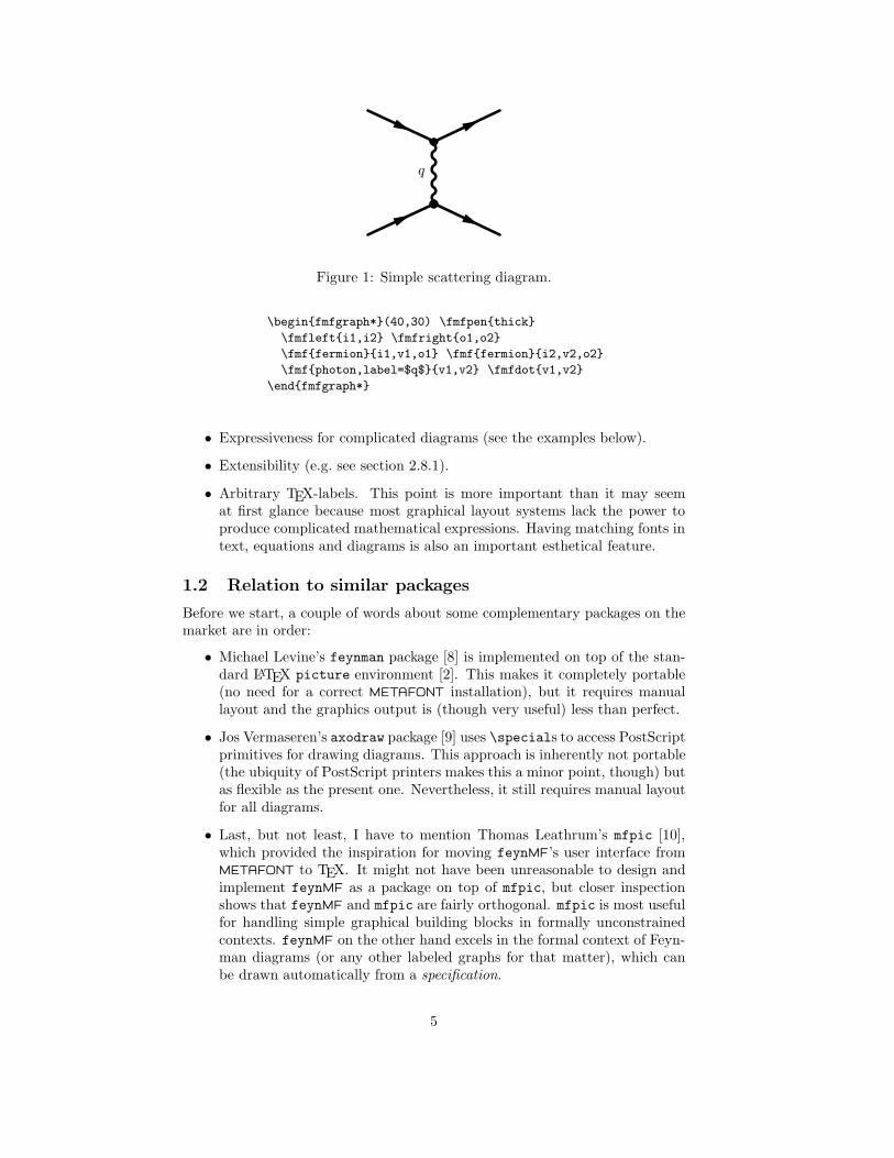
• Simplicity and conciseness for common diagrams. E.g. the scattering dia-gram in figure 1 can be specified completely in five lines of LATEX:
1TEX is a trademark of the American Mathematical Society.2LATEX might be a trademark of Addison Wesley Publishing Company.3PostScript is a trademark of Adobe Systems Inc.4METAFONT is a trademark of Addison Wesley Publishing Company.
5John Hobby’s META O T is a modified version of METAFONT which generates (encap-sulated) PostScript output. META O T can be build trivially on top of the web2c version ofTEX and METAFONT for UNIX. Ports to other systems should be simple.
6feynMF is not anybody’s trademark.
4
q
Figure 1: Simple scattering diagram.
\begin{fmfgraph*}(40,30) \fmfpen{thick}
\fmfleft{i1,i2} \fmfright{o1,o2}
\fmf{fermion}{i1,v1,o1} \fmf{fermion}{i2,v2,o2}
\fmf{photon,label=$q$}{v1,v2} \fmfdot{v1,v2}
\end{fmfgraph*}
• Expressiveness for complicated diagrams (see the examples below).
• Extensibility (e.g. see section 2.8.1).
• Arbitrary TEX-labels. This point is more important than it may seemat first glance because most graphical layout systems lack the power toproduce complicated mathematical expressions. Having matching fonts intext, equations and diagrams is also an important esthetical feature.
1.2 Relation to similar packages
Before we start, a couple of words about some complementary packages on themarket are in order:
• Michael Levine’s feynman package [8] is implemented on top of the stan-dard LATEX picture environment [2]. This makes it completely portable(no need for a correct METAFONT installation), but it requires manuallayout and the graphics output is (though very useful) less than perfect.
• Jos Vermaseren’s axodraw package [9] uses \specials to access PostScriptprimitives for drawing diagrams. This approach is inherently not portable(the ubiquity of PostScript printers makes this a minor point, though) butas flexible as the present one. Nevertheless, it still requires manual layoutfor all diagrams.
• Last, but not least, I have to mention Thomas Leathrum’s mfpic [10],which provided the inspiration for moving feynMF’s user interface fromMETAFONT to TEX. It might not have been unreasonable to design andimplement feynMF as a package on top of mfpic, but closer inspectionshows that feynMF and mfpic are fairly orthogonal. mfpic is most usefulfor handling simple graphical building blocks in formally unconstrainedcontexts. feynMF on the other hand excels in the formal context of Feyn-man diagrams (or any other labeled graphs for that matter), which canbe drawn automatically from a specification.
5
1.3 Historical note
Parts of this code have a rather long history7. Some of the drawing primitivesstarted in 1989 as feynman.mf, a library of METAFONT macros for drawingFeynman diagrams in my thesis. The layout had to be specified completely byhand, which required a long edit-process-preview cycle and made feynman.mfawkward to use. Nevertheless, it suited my and other’s neeeds and survivedfor five years without major modifications. Early in 1994, I became aware ofThomas Leathrum’s mfpic [10]. This inspired me to shift the user interfacefrom METAFONT to LATEX, because this allows a smoother blending of theLATEX picture environment with feynMF for the purpose of labeling the graphs.While doing this and after having been taught by Tim Stelzer’s and Bill Long’sMADGRAPH [11] that simply minimizing the length of the graph gives much betterresults than I had anticipated, I added the graph manipulation and layout code.
1.4 Architecture
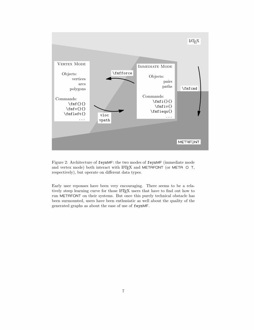
Even though there has never been a proper design phase in the development offeynMF, a certain structure has emerged, which is depicted in figure 2. A userwho is aware of this architecture should be able to use feynMF more effectively.The most crucial aspect of the architecture is the existence of two distinct modeswith different fundamental datatypes:
• vertex mode, which deals with graphs as structures consisting of verticesand arcs and (almost) never deals with their physical locations.
• immediate mode, which deals with METAFONT paths and pairs (i.e. co-ordinates) and allows complete control over the physical locations.
It is of course possible to mix these modes in advanced applications. Commandsare provided to translate vertices and arcs to pairs and paths and vice versa.Novice users with little experience in METAFONT programming should startwith vertex mode to get their job done. Later, immediate mode can be used tocreate more and more complex diagrams. It is possible to create most diagramsthat can actually be calculated in vertex mode. Immediate mode is most usefulfor extending line feynMF and for drawing diagrams with fancy decorations.A word on portability: feynMF is implemented as a LATEX package. But itshould be straightforward to adapt it to other TEX macro packages becauseLATEX macros have been used for convenience only and can easily be replaced orprovided in a compatibility package. The LATEX specific environment constructcan also easily be replaced by the equivalent construct in another macro package.
1.5 Conclusion
It goes without saying that feynMF is not perfect. There might be cases whereusing a graphical drawing tool with a mouse can give more pleasing results inless time. But in most cases, feynMF will give satisfactory results without anyfine tuning. These will be reproducible and independent from the computer itis running on.
7Which is a partial explanation, if not excuse, for its slightly incoherent structure.
6
\fmfforce
vlocvpath
\fmfcmd
Immediate Mode
Objects:pairspaths
Commands:\fmfi{}{}\fmfiv{}
\fmfiequ{}...
Vertex Mode
Objects:vertices
arcspolygons
Commands:\fmf{}{}\fmfv{}{}\fmfleft{}
...
LaTEX
METAFONT
Figure 2: Architecture of feynMF: the two modes of feynMF (immediate modeand vertex mode) both interact with LATEX and METAFONT (or META O T,respectively), but operate on different data types.
Early user reponses have been very encouraging. There seems to be a rela-tively steep learning curve for those LATEX users that have to find out how torun METAFONT on their systems. But once this purely technical obstacle hasbeen surmounted, users have been enthusiatic as well about the quality of thegenerated graphs as about the ease of use of feynMF.
7
2 Usage
In addition to this manual, there exists also a concise description of feynMF ina journal article [6], as well as a three part tutorial [7].
2.1 LATEX package and environments
Instructing LATEX to use feynMF is as simple as8
\usepackage{feynmf}
If you have META O T, then you can use it alternatively by placing
\usepackage{feynmp}
in your LATEX source.9
feynMF has to switch interactions mode and switches to \errorstopmode, be-cause it is impossible in TEX to switch back. If a different default is required (forautomated preprint processing, in particular), it can be specified as a packageoption:
\usepackage[errorstop]{feynmf}\usepackage[scroll]{feynmf}\usepackage[batch]{feynmf}\usepackage[nonstop]{feynmf}
All descriptions that should go into one METAFONT file are placed inside afmffile
fmffile environment which takes the name of the METAFONT file as an argu-ment:
\begin{fmffile}{〈METAFONT-file〉}. . .
\end{fmffile}
8As given, this applies to LATEX. But the installation file feynmf209.ins allows to generatespecial versions feynmf209.sty and feynmp209.sty which are compatible with the obsoleteLATEX version 2.09. These files are to be used as documentstyle options
\documentstyle[...,feynmf209,...]{...}or
\documentstyle[...,feynmp209,...]{...}If you cannot use epsf.sty for including PostScript files, you can either hack feynmp209.sty
or upgrade to LATEX2e. Please keep in mind that feynMF has been developed for LATEX 2εand the LATEX 2.09 compatibility version will always be a retrofitted hack. I will accept bugreports for the 2.09 version, but I urge everybody to move to LATEX2e, which is the one andonly supported LATEX right now.
9feynMF understands an option pre-1.03, that is of interest for veteran users:
\usepackage[pre-1.03]{feynmf}or
\usepackage[pre-1.03]{feynmp}The purpose of this option is to enable processing of old input files (pre v1.02) that use\noexpand in labels. Since the method for processing these files can clash (in rare cases) withLATEX 2ε’s font loading procedure, it has been disabled by default.
8
Upto 255 graphs can be placed into one METAFONT file. Currently feynMF
does not check that the 255 graph limit per file is not overrun.10 Note thatthe filename for the METAFONT file given in the argument of the fmffileenvironment must not be identical to the LATEX source file name, because theMETAFONT .log would be overwritten and LATEX can no longer access theinformation in this .log file. It should be obvious that any umber of diagramscan be generated by using more than one fmffile environment with differentfilenames.The fmfgraph environment contains the description of a single Feynman dia-fmfgraph
gram which will be placed a the location of the environment. Arguments arethe width and the height of the diagram, in units of \unitlength:
\begin{fmfgraph}(〈width〉,〈height〉). . .
\end{fmfgraph}
This environment does not support labels, use fmfgraph* if your diagramscontains labels.Same as fmfgraph, but enclosed in a picture environment of the same size andfmfgraph*
supporting LATEX labels.
\begin{fmfgraph*}(〈width〉,〈height〉). . .
\end{fmfgraph*}
Allows to allocate additional space around a fmfgraph*, since the labels (or the\fmfframe
diagram itself) might overshoot:
\fmfframe(〈left〉,〈top〉)(〈right〉,〈bottom〉){〈box 〉}
puts an invisible frame of the given dimensions (measured in \unitlength)around 〈box 〉.
2.2 Auxiliary files
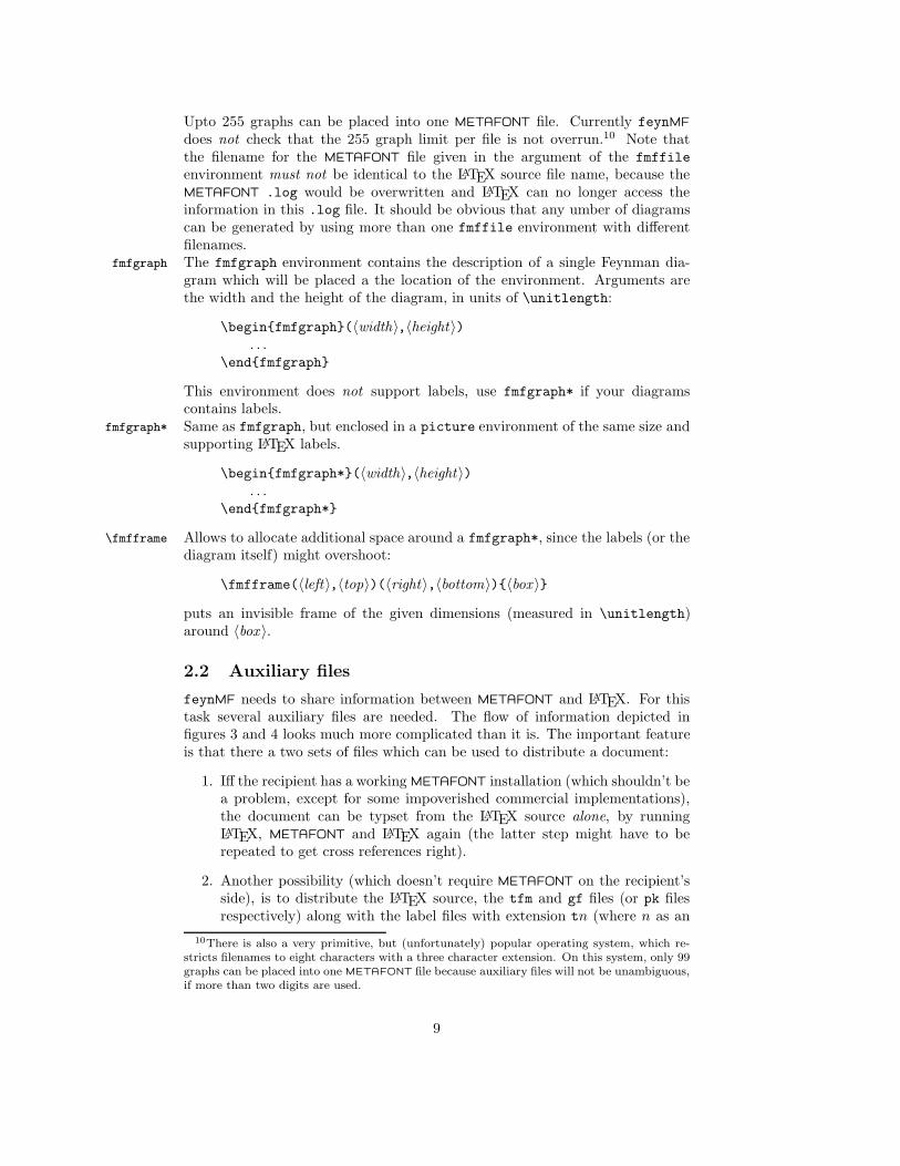
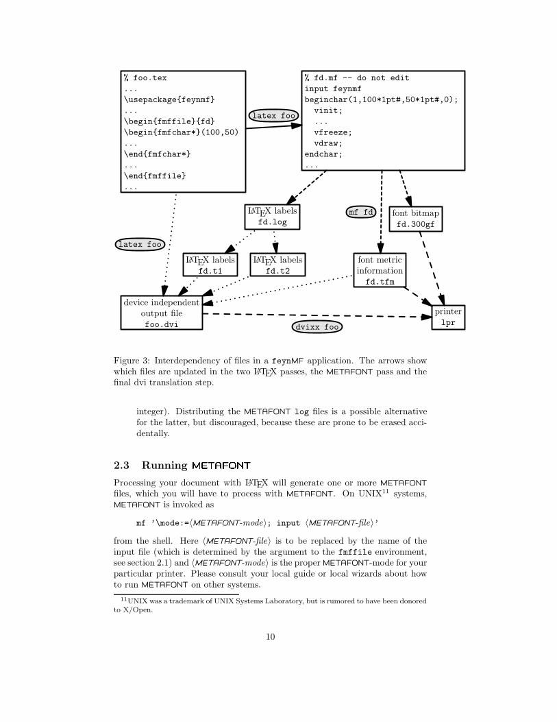
feynMF needs to share information between METAFONT and LATEX. For thistask several auxiliary files are needed. The flow of information depicted infigures 3 and 4 looks much more complicated than it is. The important featureis that there a two sets of files which can be used to distribute a document:
1. Iff the recipient has a working METAFONT installation (which shouldn’t bea problem, except for some impoverished commercial implementations),the document can be typset from the LATEX source alone, by runningLATEX, METAFONT and LATEX again (the latter step might have to berepeated to get cross references right).
2. Another possibility (which doesn’t require METAFONT on the recipient’sside), is to distribute the LATEX source, the tfm and gf files (or pk filesrespectively) along with the label files with extension tn (where n as an
10There is also a very primitive, but (unfortunately) popular operating system, which re-stricts filenames to eight characters with a three character extension. On this system, only 99graphs can be placed into one METAFONT file because auxiliary files will not be unambiguous,if more than two digits are used.
9
% foo.tex...\usepackage{feynmf}...\begin{fmffile}{fd}\begin{fmfchar*}(100,50)...\end{fmfchar*}...\end{fmffile}...
% fd.mf -- do not editinput feynmfbeginchar(1,100*1pt#,50*1pt#,0);
vinit;...vfreeze;vdraw;
endchar;...
LaTEX labelsfd.log
font metricinformationfd.tfm
font bitmapfd.300gf
LaTEX labelsfd.t1
LaTEX labelsfd.t2
device independentoutput filefoo.dvi
printerlpr
latex foo
latex foo
mf fd
dvixx foo
Figure 3: Interdependency of files in a feynMF application. The arrows showwhich files are updated in the two LATEX passes, the METAFONT pass and thefinal dvi translation step.
integer). Distributing the METAFONT log files is a possible alternativefor the latter, but discouraged, because these are prone to be erased acci-dentally.
2.3 Running METAFONT
Processing your document with LATEX will generate one or more METAFONT
files, which you will have to process with METAFONT. On UNIX11 systems,METAFONT is invoked as
mf ’\mode:=〈METAFONT-mode〉; input 〈METAFONT-file〉’
from the shell. Here 〈METAFONT-file〉 is to be replaced by the name of theinput file (which is determined by the argument to the fmffile environment,see section 2.1) and 〈METAFONT-mode〉 is the proper METAFONT-mode for yourparticular printer. Please consult your local guide or local wizards about howto run METAFONT on other systems.
11UNIX was a trademark of UNIX Systems Laboratory, but is rumored to have been donoredto X/Open.
10
% foo.tex...\usepackage{feynmp}...\begin{fmffile}{fd}\begin{fmfchar*}(100,50)...\end{fmfchar*}...\end{fmffile}...
% fd.mp -- do not editinput feynmpbeginchar(1,100*1pt#,50*1pt#,0);
vinit;...vfreeze;vdraw;
endchar;...
LaTEX labelsfd.t1
LaTEX labelsfd.t2
encapsulatedPostScript
filefd.1
encapsulatedPostScript
filefd.2
device independentoutput filefoo.dvi
printerlpr
latex foo
latex foo
mp fd
dvixx foo
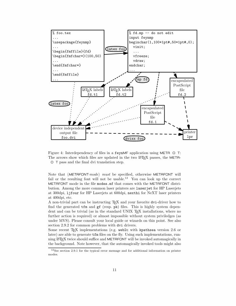
Figure 4: Interdependency of files in a feynMF application using META O T:The arrows show which files are updated in the two LATEX passes, the META-
O T pass and the final dvi translation step.
Note that 〈METAFONT-mode〉 must be specified, otherwise METAFONT willfail or the resulting font will not be usable.12 You can look up the correctMETAFONT mode in the file modes.mf that comes with the METAFONT distri-bution. Among the more common laser printers are laserjet for HP Laserjetsat 300dpi, ljfour for HP Laserjets at 600dpi, nexthi for NeXT laser printersat 400dpi, etc.A non-trivial part can be instructing TEX and your favorite dvi-driver how tofind the generated tfm and gf (resp. pk) files. This is highly system depen-dent and can be trivial (as in the standard UNIX TEX installations, where nofurther action is required) or almost impossible without system priviledges (asunder MVS). Please consult your local guide or wizards on this point. See alsosection 2.9.2 for common problems with dvi drivers.Some recent TEX implementations (e.g. web2c with kpathsea version 2.6 orlater) are able to generate tfm files on the fly. Using such implementations, run-ning LATEX twice should suffice and METAFONT will be invoked automagically inthe background. Note however, that the automagically invoked tools might also
12See section 2.9.1 for the typical error message and for additional information on printermodes.
11
install the “fonts” corresponding to the Feynman diagrams in a system direc-tory, where they don’t belong. Adding the following lines to the maketex.sitescript will prevent this mishap in the teTEX distribution for UNIX (which isderived from web2c):
if [ -r $KPSE_DOT/$NAME.mf ]; then
MT_PKDESTDIR=$KPSE_DOT
MT_TFMDESTDIR=$KPSE_DOT
MT_NAMEPART=
fi
The automagic tools will also not notice when a diagram has changed. Theseproblems suggest that it is a generally a good idea to invoke METAFONT ex-plicitely, instead of relying on the automagic tools.Running META O T is usually trivial, because not printer specific mode isneeded:
mp 〈META O T-file〉
2.4 The feynmf perl script
UNIX users will be able to take advantage of the feynmf perl script, that auto-mates the invocation of LATEX and META O T. In particular it tries to guessthe correct METAFONT-mode and magnification. The latter is often differentfrom 1 in slide classes. Here is the man page of feynmf:
NAME
feynmf — Process LaTeX files using FeynMF
SYNOPSIS
feynmf [-hvqncfT] [-t tfm [-t tfm ...]] [-m mode] file [file ...]feynmf [--help] [--version] [--quiet] [--noexec] [--clean] [--force][--notfm] [--tfm tfm [--tfm tfm ...]] [--mode mode] file [file ...]
DESCRIPTION
The most complicated part of using the FeynMF style appears to be the properinvocation of Metafont. The feynmf script provides a convenient front end andwill automagically invoke Metafont with the proper mode and magnifincation.It will also avoid cluttering system font directories and offers an option to cleanthem.
OPTIONS
-h, --helpPrint a short help text.
-v, --versionPrint the version of feynmf.
12
-q, --quietDon’t echo the commands being executed.
-n, --noexecDon’t execute LaTeX or Metafont.
-c, --cleanOffer to delete font files that have accidentally been placed in a system di-rectory by the MakeTeXTFM and MakeTeXPK scripts (these scriptsare run by tex (and latex) in the background). This option has only beentested with recent versions of UNIX TeX.
-f, --forceDon’t ask any questions.
-T, --notfmDon’t try to prepare fake .tfm files for the first run.
-t, --tfm tfmDon’t try guess the names of the .tfm files to fake for the first run anduse the given name(s) instead. This option can be useful if our incompleteparsing of the LaTeX input files fails.
-m mode, --mode modeSelect the METAFONT mode mode. The default is guessed or localfontif the guess fails.
fileMain LaTeX input files.
file ...Other LaTeX input files that are included by the main file.
AUTHOR
Thorsten Ohl <[email protected]>
BUGS
The preparation of .tfm files is not foolproof yet, because we can parse TeXfiles only superficially.This script has only been tested for recent teTeX distributions of UNIX TeX,though it will probably work with other versions of UNIX TeX. The author willbe grateful for portability suggestions, even concerning Borg operating systems,for the benefit of those users that are forced to live with DOS or Windows.
2.5 Vertex mode
These basic features of feynMF are (or rather “should be”) available throughthe LATEX interface. No knowledge of METAFONT is necessary.
13
v1 v2 v3v4 v1
v2
v3
v4
v1
v2v3
v4
v5
v6v7
v1v2 v3 v4
v1
v2
v3
v4
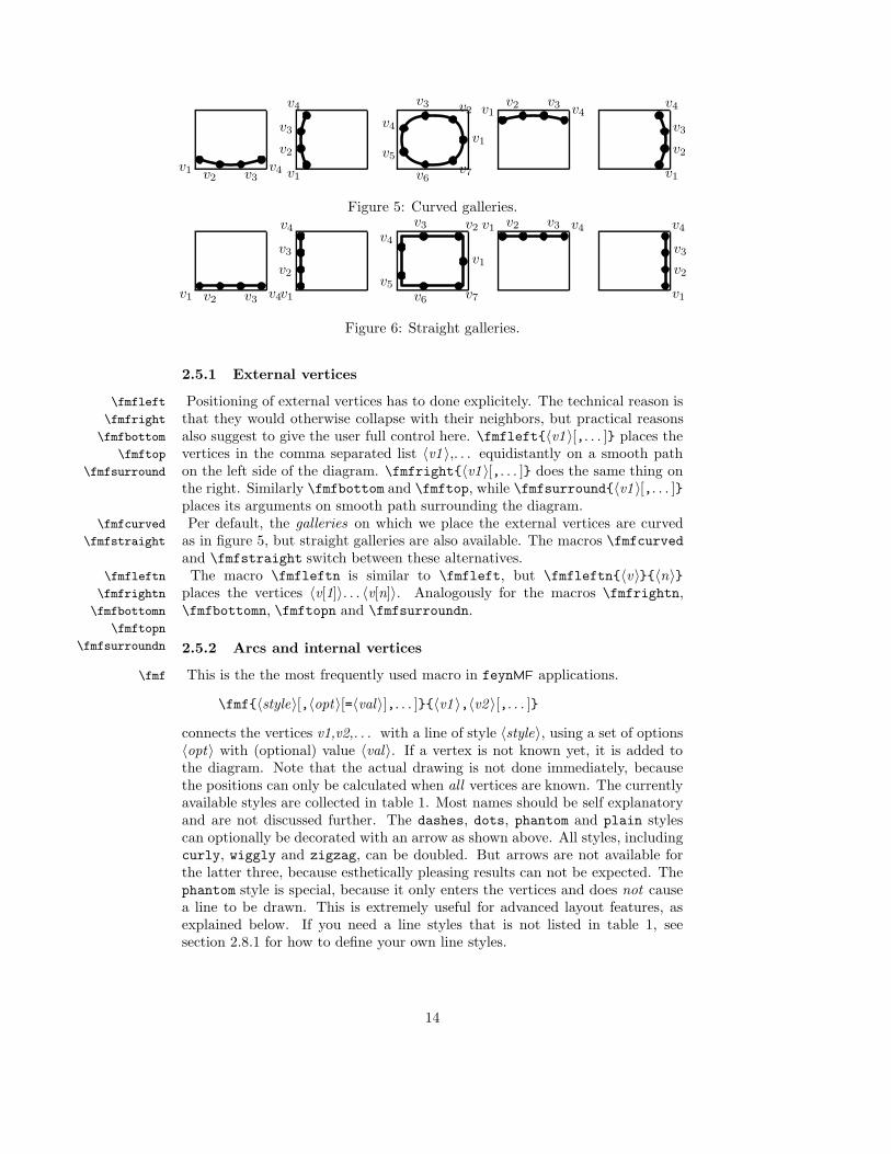
Figure 5: Curved galleries.
v1 v2 v3 v4v1
v2
v3
v4
v1
v2v3
v4
v5
v6 v7
v1 v2 v3 v4
v1
v2
v3
v4
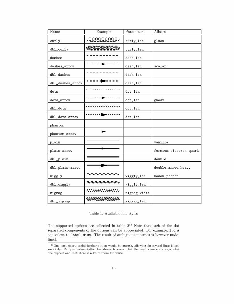
Figure 6: Straight galleries.
2.5.1 External vertices
Positioning of external vertices has to done explicitely. The technical reason is\fmfleft
\fmfright
\fmfbottom
\fmftop
\fmfsurround
that they would otherwise collapse with their neighbors, but practical reasonsalso suggest to give the user full control here. \fmfleft{〈v1 〉[,. . . ]} places thevertices in the comma separated list 〈v1 〉,. . . equidistantly on a smooth pathon the left side of the diagram. \fmfright{〈v1 〉[,. . . ]} does the same thing onthe right. Similarly \fmfbottom and \fmftop, while \fmfsurround{〈v1 〉[,. . . ]}places its arguments on smooth path surrounding the diagram.Per default, the galleries on which we place the external vertices are curved\fmfcurved
\fmfstraight as in figure 5, but straight galleries are also available. The macros \fmfcurvedand \fmfstraight switch between these alternatives.
The macro \fmfleftn is similar to \fmfleft, but \fmfleftn{〈v〉}{〈n〉}\fmfleftn
\fmfrightn
\fmfbottomn
\fmftopn
\fmfsurroundn
places the vertices 〈v[1]〉. . . 〈v[n]〉. Analogously for the macros \fmfrightn,\fmfbottomn, \fmftopn and \fmfsurroundn.
2.5.2 Arcs and internal vertices
This is the the most frequently used macro in feynMF applications.\fmf
\fmf{〈style〉[,〈opt〉[=〈val〉],. . . ]}{〈v1 〉,〈v2 〉[,. . . ]}
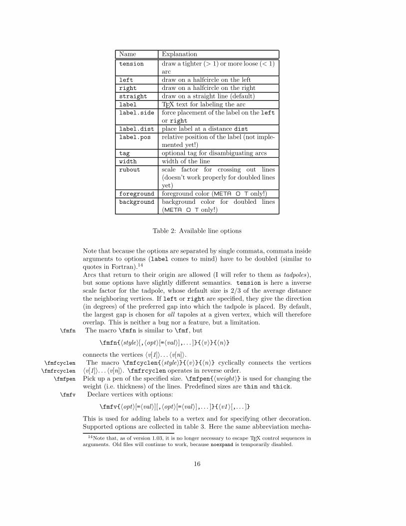
connects the vertices v1,v2,. . . with a line of style 〈style〉, using a set of options〈opt〉 with (optional) value 〈val〉. If a vertex is not known yet, it is added tothe diagram. Note that the actual drawing is not done immediately, becausethe positions can only be calculated when all vertices are known. The currentlyavailable styles are collected in table 1. Most names should be self explanatoryand are not discussed further. The dashes, dots, phantom and plain stylescan optionally be decorated with an arrow as shown above. All styles, includingcurly, wiggly and zigzag, can be doubled. But arrows are not available forthe latter three, because esthetically pleasing results can not be expected. Thephantom style is special, because it only enters the vertices and does not causea line to be drawn. This is extremely useful for advanced layout features, asexplained below. If you need a line styles that is not listed in table 1, seesection 2.8.1 for how to define your own line styles.
14
Name Example Parameters Aliases
curly curly_len gluon
dbl_curly curly_len
dashes dash_len
dashes_arrow dash_len scalar
dbl_dashes dash_len
dbl_dashes_arrow dash_len
dots dot_len
dots_arrow dot_len ghost
dbl_dots dot_len
dbl_dots_arrow dot_len
phantom
phantom_arrow
plain vanilla
plain_arrow fermion, electron, quark
dbl_plain double
dbl_plain_arrow double_arrow, heavy
wiggly wiggly_len boson, photon
dbl_wiggly wiggly_len
zigzag zigzag_width
dbl_zigzag zigzag_len
Table 1: Available line styles
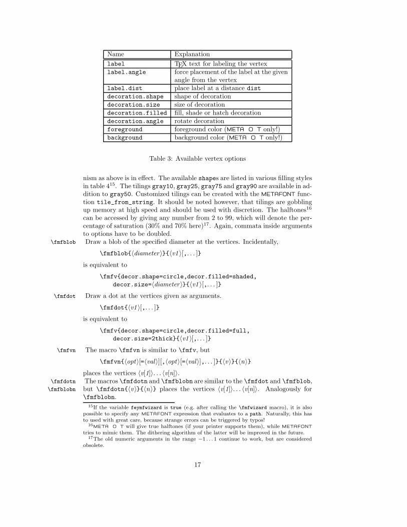
The supported options are collected in table 213 Note that each of the dotseparated components of the options can be abbreviated. For example, l.d isequivalent to label.dist. The result of ambiguous matches is however unde-fined.
13One particulary useful further option would be smooth, allowing for several lines joinedsmoothly. Early experimentation has shown however, that the results are not always whatone expects and that there is a lot of room for abuse.
15
Name Explanationtension draw a tighter (> 1) or more loose (< 1)
arcleft draw on a halfcircle on the leftright draw on a halfcircle on the rightstraight draw on a straight line (default)label TEX text for labeling the arclabel.side force placement of the label on the left
or rightlabel.dist place label at a distance distlabel.pos relative position of the label (not imple-
mented yet!)tag optional tag for disambiguating arcswidth width of the linerubout scale factor for crossing out lines
(doesn’t work properly for doubled linesyet)
foreground foreground color (META O T only!)background background color for doubled lines
(META O T only!)
Table 2: Available line options
Note that because the options are separated by single commata, commata insidearguments to options (label comes to mind) have to be doubled (similar toquotes in Fortran).14
Arcs that return to their origin are allowed (I will refer to them as tadpoles),but some options have slightly different semantics. tension is here a inversescale factor for the tadpole, whose default size is 2/3 of the average distancethe neighboring vertices. If left or right are specified, they give the direction(in degrees) of the preferred gap into which the tadpole is placed. By default,the largest gap is chosen for all tapoles at a given vertex, which will thereforeoverlap. This is neither a bug nor a feature, but a limitation.The macro \fmfn is similar to \fmf, but\fmfn
\fmfn{〈style〉[,〈opt〉[=〈val〉],. . . ]}{〈v〉}{〈n〉}
connects the vertices 〈v[1]〉. . . 〈v[n]〉.The macro \fmfcyclen{〈style〉}{〈v〉}{〈n〉} cyclically connects the vertices\fmfcyclen
\fmfrcyclen 〈v[1]〉. . . 〈v[n]〉. \fmfrcyclen operates in reverse order.Pick up a pen of the specified size. \fmfpen{〈weight〉} is used for changing the\fmfpen
weight (i.e. thickness) of the lines. Predefined sizes are thin and thick.Declare vertices with options:\fmfv
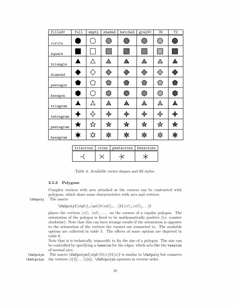
\fmfv{〈opt〉[=〈val〉][,〈opt〉[=〈val〉],. . . ]}{〈v1 〉[,. . . ]}
This is used for adding labels to a vertex and for specifying other decoration.Supported options are collected in table 3. Here the same abbreviation mecha-
14Note that, as of version 1.03, it is no longer necessary to escape TEX control sequences inarguments. Old files will continue to work, because noexpand is temporarily disabled.
16
Name Explanationlabel TEX text for labeling the vertexlabel.angle force placement of the label at the given
angle from the vertexlabel.dist place label at a distance distdecoration.shape shape of decorationdecoration.size size of decorationdecoration.filled fill, shade or hatch decorationdecoration.angle rotate decorationforeground foreground color (META O T only!)background background color (META O T only!)
Table 3: Available vertex options
nism as above is in effect. The available shapes are listed in various filling stylesin table 415. The tilings gray10, gray25, gray75 and gray90 are available in ad-dition to gray50. Customized tilings can be created with the METAFONT func-tion tile_from_string. It should be noted however, that tilings are gobblingup memory at high speed and should be used with discretion. The halftones16
can be accessed by giving any number from 2 to 99, which will denote the per-centage of saturation (30% and 70% here)17. Again, commata inside argumentsto options have to be doubled.Draw a blob of the specified diameter at the vertices. Incidentally,\fmfblob
\fmfblob{〈diameter〉}{〈v1 〉[,. . . ]}
is equivalent to
\fmfv{decor.shape=circle,decor.filled=shaded,decor.size=〈diameter〉}{〈v1 〉[,. . . ]}
Draw a dot at the vertices given as arguments.\fmfdot
\fmfdot{〈v1 〉[,. . . ]}
is equivalent to
\fmfv{decor.shape=circle,decor.filled=full,decor.size=2thick}{〈v1 〉[,. . . ]}
The macro \fmfvn is similar to \fmfv, but\fmfvn
\fmfvn{〈opt〉[=〈val〉][,〈opt〉[=〈val〉],. . . ]}{〈v〉}{〈n〉}places the vertices 〈v[1]〉. . . 〈v[n]〉.The macros \fmfdotn and \fmfblobn are similar to the \fmfdot and \fmfblob,\fmfdotn
\fmfblobn but \fmfdotn{〈v〉}{〈n〉} places the vertices 〈v[1]〉. . . 〈v[n]〉. Analogously for\fmfblobn.
15If the variable feymfwizard is true (e.g. after calling the \fmfwizard macro), it is alsopossible to specify any METAFONT expression that evaluates to a path. Naturally, this hasto used with great care, because strange errors can be triggered by typos!
16META O T will give true halftones (if your printer supports them), while METAFONT
tries to mimic them. The dithering algorithm of the latter will be improved in the future.17The old numeric arguments in the range −1 . . . 1 continue to work, but are considered
obsolete.
17
filled= full empty shaded hatched gray50 30 70
circle
square
triangle
diamond
pentagon
hexagon
triagram
tetragram
pentagram
hexagram
triacross cross pentacross hexacross
Table 4: Available vertex shapes and fill styles.
2.5.3 Polygons
Complex vertices with arcs attached at the corners can be contructed withpolygons, which share some characteristics with arcs and vertices.The macro\fmfpoly
\fmfpoly{〈style〉[,〈opt〉[=〈val〉],. . . ]}{〈v1 〉,〈v2 〉[,. . . ]}
places the vertices 〈v1 〉, 〈v2 〉, . . . on the corners of a regular polygon. Theorientation of the polygon is fixed to be mathematically positive (i.e. counterclockwise). Note that this can have strange results if the orientation is oppositeto the orientation of the vertices the corners are connected to. The availableoptions are collected in table 5. The effects of some options are depicted intable 6.Note that is is technically impossible to fix the size of a polygon. The size canbe controlled by specifying a tension for the edges, which acts like the tensionof normal arcs.The macro \fmfpolyn{〈style〉}{〈v〉}{〈n〉} is similar to \fmfpoly but connects\fmfpolyn
\fmfrpolyn the vertices 〈v[1]〉. . . 〈v[n]〉. \fmfrpolyn operates in reverse order.
18
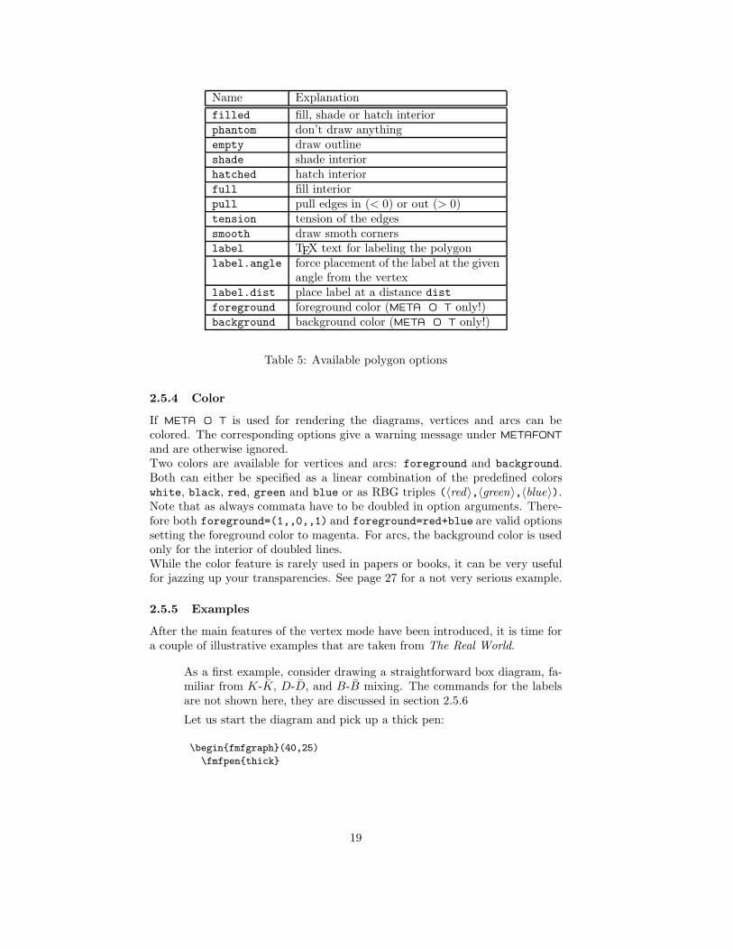
Name Explanationfilled fill, shade or hatch interiorphantom don’t draw anythingempty draw outlineshade shade interiorhatched hatch interiorfull fill interiorpull pull edges in (< 0) or out (> 0)tension tension of the edgessmooth draw smoth cornerslabel TEX text for labeling the polygonlabel.angle force placement of the label at the given
angle from the vertexlabel.dist place label at a distance distforeground foreground color (META O T only!)background background color (META O T only!)
Table 5: Available polygon options
2.5.4 Color
If META O T is used for rendering the diagrams, vertices and arcs can becolored. The corresponding options give a warning message under METAFONT
and are otherwise ignored.Two colors are available for vertices and arcs: foreground and background.Both can either be specified as a linear combination of the predefined colorswhite, black, red, green and blue or as RBG triples (〈red〉,〈green〉,〈blue〉).Note that as always commata have to be doubled in option arguments. There-fore both foreground=(1,,0,,1) and foreground=red+blue are valid optionssetting the foreground color to magenta. For arcs, the background color is usedonly for the interior of doubled lines.While the color feature is rarely used in papers or books, it can be very usefulfor jazzing up your transparencies. See page 27 for a not very serious example.
2.5.5 Examples
After the main features of the vertex mode have been introduced, it is time fora couple of illustrative examples that are taken from The Real World.
As a first example, consider drawing a straightforward box diagram, fa-miliar from K-K, D-D, and B-B mixing. The commands for the labelsare not shown here, they are discussed in section 2.5.6
Let us start the diagram and pick up a thick pen:
\begin{fmfgraph}(40,25)
\fmfpen{thick}
19
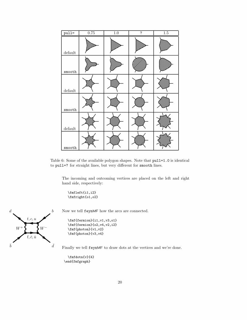
pull= 0.75 1.0 ? 1.5
default
smooth
default
smooth
default
smooth
Table 6: Some of the available polygon shapes. Note that pull=1.0 is identicalto pull=? for straight lines, but very different for smooth lines.
The incoming and outcoming vertices are placed on the left and righthand side, respectively:
\fmfleft{i1,i2}
\fmfright{o1,o2}
Now we tell feynMF how the arcs are connected.
\fmf{fermion}{i1,v1,v3,o1}
\fmf{fermion}{o2,v4,v2,i2}
\fmf{photon}{v1,v2}
\fmf{photon}{v3,v4}t, c, u
W+ W−
t, c, u
b
d
d
b
Finally we tell feynMF to draw dots at the vertices and we’re done.
\fmfdotn{v}{4}
\end{fmfgraph}
20

With a little effort the layout of this diagram can actually be improvedby enlarging the inner box, see page 29 below.
Here is the resonant s-channel contribution to e+e− → 4f . (From nowon, we do no longer display the
\begin{fmfgraph}(40,25)
\fmfpen{thick}
...
\end{fmfgraph}
environment surrounding all pictures.)
\fmfleftn{i}{2}
\fmfrightn{o}{4}
\fmf{fermion}{i1,v1,i2}
\fmf{photon}{v1,v2}
\fmfblob{.15w}{v2}
\fmf{photon}{v2,v3}
\fmf{fermion}{o1,v3,o2}
\fmf{photon}{v2,v4}
\fmf{fermion}{o4,v4,o3}
e−
e+
µ+
νµ
s
c
And the resonant t-channel contribution:
\fmfleftn{i}{2}
\fmfrightn{o}{4}
\fmf{fermion}{i1,v1,v2,i2}
\fmf{photon}{v1,v3}
\fmf{fermion}{o1,v3,o2}
\fmf{photon}{v2,v4}
\fmf{fermion}{o4,v4,o3}
e−
e+
µ+
νµ
s
c
Two point loop diagrams pose another set of problems. We must havea way of specifying that one or more of the lines connecting the twovertices are not connected by a straight line. The options left, rightand straight offer the possibility to connect two vertices by a semicircledetour, either on the left or on the right. Since by default all lines con-tribute to the tension between two vertices, the tension option allows usto reduce this tension. The next examples shows both options in action.The lower fermion line is given an tension of 1/3 to make is symmetricalwith the upper line with consists of three parts. The loop photon is usinga detour on the right and does not contribute any tension.
\fmfleft{i1,i2}
\fmfright{o1}
\fmf{fermion,tension=1/3}{i1,v1}
\fmf{plain}{v1,v2}
\fmf{fermion}{v2,v3}
\fmf{photon,right,tension=0}{v2,v3}
21
\fmf{plain}{v3,i2}
\fmf{photon}{v1,o1}
p− k
k
p′
p
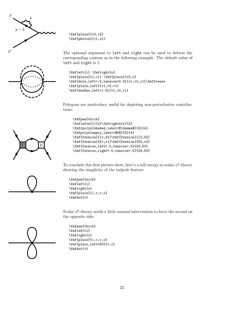
The optional argument to left and right can be used to deform thecorresponding contour as in the following example. The default value ofleft and right is 1.
\fmfleft{i} \fmfright{o}
\fmf{plain}{i,v1} \fmf{plain}{v2,o}
\fmf{dots,left=.5,tension=0.3}{v1,v2,v1}\fmffreeze
\fmf{plain,left}{v1,v2,v1}
\fmf{dashes,left=1.5}{v1,v2,v1}
Polygons are particulary useful for depicting non-perturbative contribu-tions:
\fmfpen{thick}
\fmfleftn{l}{2}\fmfrightn{r}{2}
\fmfrpolyn{shaded,label=$\Gamma$}{G}{4}
\fmfpolyn{empty,label=$K$}{K}{4}
\fmf{fermion}{l1,G1}\fmf{fermion}{l2,G2}
\fmf{fermion}{K1,r1}\fmf{fermion}{K2,r2}
\fmf{fermion,left=.5,tension=.5}{G3,K3}
\fmf{fermion,right=.5,tension=.5}{G4,K4}
Γ K
To conclude this first picture show, here’s a self energy in scalar φ4-theoryshowing the simplicity of the tadpole feature:
\fmfpen{thick}
\fmfleft{i}
\fmfright{o}
\fmf{plain}{i,v,v,o}
\fmfdot{v}
Scalar φ6-theory needs a little manual intervention to force the second onthe opposite side:
\fmfpen{thick}
\fmfleft{i}
\fmfright{o}
\fmf{plain}{i,v,v,o}
\fmf{plain,left=90}{v,v}
\fmfdot{v}
22
2.5.6 Labels
Let us now come back to the examples on page 21 and discuss how to add thelabels.The macro\fmflabel
\fmflabel{〈label〉}{〈v〉}
is equivalent to
\fmfv{label=〈label〉}{〈v〉}
and adds the label 〈label〉 to the vertex 〈v〉. In the current implementation, therecan be only a single label for each vertex. Thus earlier calls to \fmflabel for thesame vertex will be overwritten. 〈label〉 will be placed with the \put commandof the LATEX picture environment.18 Note that the fmfgraph* environmentmust be used to use labels, they will silently disappear in fmfgraph.\fmflabel gives the user no control on the placement of the the label (use the\fmfv macro for a more fine-grained control). The label is placed using thefollowing algorithm:
1. The reference point of the box containing 〈label〉 is placed at the distance3thick on the continuation of the straight line connecting the center ofthe picture with the vertex 〈v〉.
2. The reference point of the box is chosen such that the contents of the boxis on the outside of the vertex (with respect to the center of the diagram).It is chosen from the four corners and the four midpoints of the sides.
Therefore the four external particles in the B-B mixing diagram on page 21 arelabelled simply by:
\fmflabel{$\bar{b}$}{i1}
\fmflabel{$d$}{i2}
\fmflabel{$\bar{d}$}{o1}
\fmflabel{$b$}{o2}
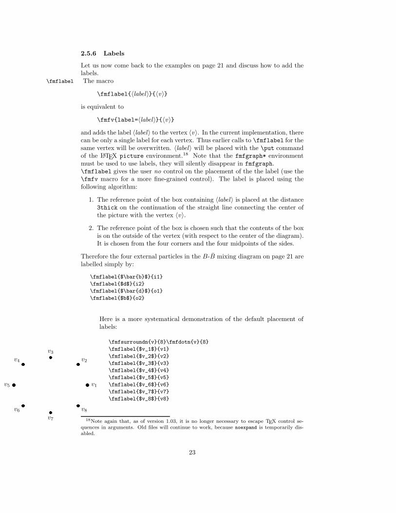
Here is a more systematical demonstration of the default placement oflabels:
\fmfsurroundn{v}{8}\fmfdotn{v}{8}
\fmflabel{$v_1$}{v1}
\fmflabel{$v_2$}{v2}
\fmflabel{$v_3$}{v3}
\fmflabel{$v_4$}{v4}
\fmflabel{$v_5$}{v5}
\fmflabel{$v_6$}{v6}
\fmflabel{$v_7$}{v7}
\fmflabel{$v_8$}{v8}
v1
v2
v3
v4
v5
v6
v7
v8
18Note again that, as of version 1.03, it is no longer necessary to escape TEX control se-quences in arguments. Old files will continue to work, because noexpand is temporarily dis-abled.
23
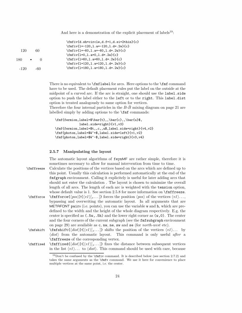
And here is a demonstration of the explicit placement of labels19:
\fmfiv{d.sh=circle,d.f=1,d.si=2thin}{c}
\fmfiv{l=-120,l.a=-120,l.d=.2w}{c}
\fmfiv{l=-60,l.a=-60,l.d=.2w}{c}
\fmfiv{l=0,l.a=0,l.d=.2w}{c}
\fmfiv{l=60,l.a=60,l.d=.2w}{c}
\fmfiv{l=120,l.a=120,l.d=.2w}{c}
\fmfiv{l=180,l.a=180,l.d=.2w}{c}-120 -60
0
60120
180
There is no equivalent to \fmflabel for arcs. Here options to the \fmf commandhave to be used. The default placement rules put the label on the outside at themidpoint of a curved arc. If the arc is straight, one should use the label.sideoption to push the label either to the left or to the right. This label.distoption is treated analogously to same option for vertices.Therefore the four internal particles in the B-B mixing diagram on page 21 arelabelled simply by adding options to the \fmf commands:
\fmf{fermion,label=$\bar{t},,\bar{c},,\bar{u}$,
label.side=right}{v1,v3}
\fmf{fermion,label=$t,,c,,u$,label.side=right}{v4,v2}
\fmf{photon,label=$W^+$,label.side=left}{v1,v2}
\fmf{photon,label=$W^-$,label.side=right}{v3,v4}
2.5.7 Manipulating the layout
The automatic layout algorithms of feynMF are rather simple, therefore it issometimes necessary to allow for manual intervention from time to time.Calculate the positions of the vertices based on the arcs which are defined up to\fmffreeze
this point. Usually this calculation is performed automatically at the end of thefmfgraph environment. Calling it explicitely is useful for later adding arcs thatshould not enter the calculation . The layout is chosen to minimize the overalllength of all arcs. The length of each arc is weighted with the tension option,whose default value is 1. See section 2.5.8 for more information on \fmffreeze.\fmfforce{〈pos〉}{〈v1 〉[,. . . ]} forces the position 〈pos〉 of the vertices 〈v1 〉. . . ,\fmfforce
bypassing and overwriting the automatic layout. In all arguments that areMETAFONT pairs (i.e. points), you can use the variable w and h, which are pre-defined to the width and the height of the whole diagram respectively. E.g. thecenter is specified as (.5w,.5h) and the lower right corner as (w,0). The centerand the four corners of the current subgraph (see the fmfsubgraph environmenton page 29) are available as c, nw, ne, sw and se (for north-west etc).\fmfshift{〈dist〉}{〈v1 〉[,. . . ]} shifts the position of the vertices 〈v1 〉. . . by\fmfshift
〈dist〉 from the automatic layout. This command is only useful after a\fmffreeze of the corresponding vertex.\fmffixed{〈dist〉}{〈v1 〉[,. . . ]} fixes the distance between subsequent vertices\fmffixed
in the list 〈v1 〉. . . to 〈dist〉. This command should be used with care, because
19Don’t be confused by the \fmfiv command. It is described below (see section 2.7.2) andtakes the same arguments as the \fmfv command. We use it here for convenience to placemultiple vertices at the same point, i.e. the center.
24
it is possible to overconstrain the layout of the graph and the error messageswill be obscure for a novice user.\fmffixedx{〈dx 〉}{〈v1 〉[,. . . ]} is identical to \fmffixed{(〈dx 〉,whatever)}{〈v1 〉\fmffixedx
\fmffixedy [,. . . ]} and \fmffixedy{〈dy〉}{〈v1 〉[,. . . ]} is identical to \fmffixed{(whatever,〈dy〉)}{〈v1 〉[,. . . ]}. These commands can be used to fix relative positions in one coordinate,while allowing movement in the other coordinate.
2.5.8 Skeletons
The single most powerful concept for adjusting feynMF’s layout decisions is theuse of skeletons. By issuing a \fmffreeze after specifying a subgraph (skeleton),we can fix the location of the skeleton as if the other arcs were not there. Wecan then successively add more subgraphs whose layout will be chosen with theskeleton remaining fixed. Similar effects can be achieved by giving some arcs avanishing tension.
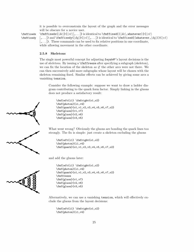
Consider the following example: suppose we want to draw a ladder dia-gram contributing to the quark form factor. Simply linking in the gluonsdoes not produce a satisfactory result:
\fmfleft{i1} \fmfright{o1,o2}
\fmf{photon}{i1,v4}
\fmf{quark}{o1,v1,v2,v3,v4,v5,v6,v7,o2}
\fmf{gluon}{v1,v7}
\fmf{gluon}{v2,v6}
\fmf{gluon}{v3,v5}
What went wrong? Obviously the gluons are bonding the quark lines toostrongly. The fix is simple: just create a skeleton excluding the gluons
\fmfleft{i1} \fmfright{o1,o2}
\fmf{photon}{i1,v4}
\fmf{quark}{o1,v1,v2,v3,v4,v5,v6,v7,o2}
and add the gluons later:
\fmfleft{i1} \fmfright{o1,o2}
\fmf{photon}{i1,v4}
\fmf{quark}{o1,v1,v2,v3,v4,v5,v6,v7,o2}
\fmffreeze
\fmf{gluon}{v1,v7}
\fmf{gluon}{v2,v6}
\fmf{gluon}{v3,v5}
Alternatively, we can use a vanishing tension, which will effectively ex-clude the gluons from the layout decisions:
\fmfleft{i1} \fmfright{o1,o2}
\fmf{photon}{i1,v4}
25
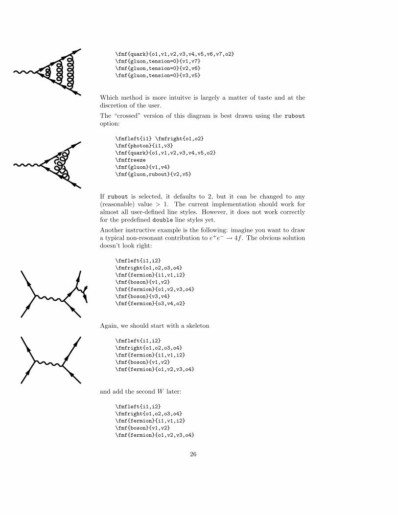
\fmf{quark}{o1,v1,v2,v3,v4,v5,v6,v7,o2}
\fmf{gluon,tension=0}{v1,v7}
\fmf{gluon,tension=0}{v2,v6}
\fmf{gluon,tension=0}{v3,v5}
Which method is more intuitve is largely a matter of taste and at thediscretion of the user.
The “crossed” version of this diagram is best drawn using the ruboutoption:
\fmfleft{i1} \fmfright{o1,o2}
\fmf{photon}{i1,v3}
\fmf{quark}{o1,v1,v2,v3,v4,v5,o2}
\fmffreeze
\fmf{gluon}{v1,v4}
\fmf{gluon,rubout}{v2,v5}
If rubout is selected, it defaults to 2, but it can be changed to any(reasonable) value > 1. The current implementation should work foralmost all user-defined line styles. However, it does not work correctlyfor the predefined double line styles yet.
Another instructive example is the following: imagine you want to drawa typical non-resonant contribution to e+e− → 4f . The obvious solutiondoesn’t look right:
\fmfleft{i1,i2}
\fmfright{o1,o2,o3,o4}
\fmf{fermion}{i1,v1,i2}
\fmf{boson}{v1,v2}
\fmf{fermion}{o1,v2,v3,o4}
\fmf{boson}{v3,v4}
\fmf{fermion}{o3,v4,o2}
Again, we should start with a skeleton
\fmfleft{i1,i2}
\fmfright{o1,o2,o3,o4}
\fmf{fermion}{i1,v1,i2}
\fmf{boson}{v1,v2}
\fmf{fermion}{o1,v2,v3,o4}
and add the second W later:
\fmfleft{i1,i2}
\fmfright{o1,o2,o3,o4}
\fmf{fermion}{i1,v1,i2}
\fmf{boson}{v1,v2}
\fmf{fermion}{o1,v2,v3,o4}
26
\fmffreeze
\fmf{boson}{v3,v4}
\fmf{fermion}{o3,v4,o2}
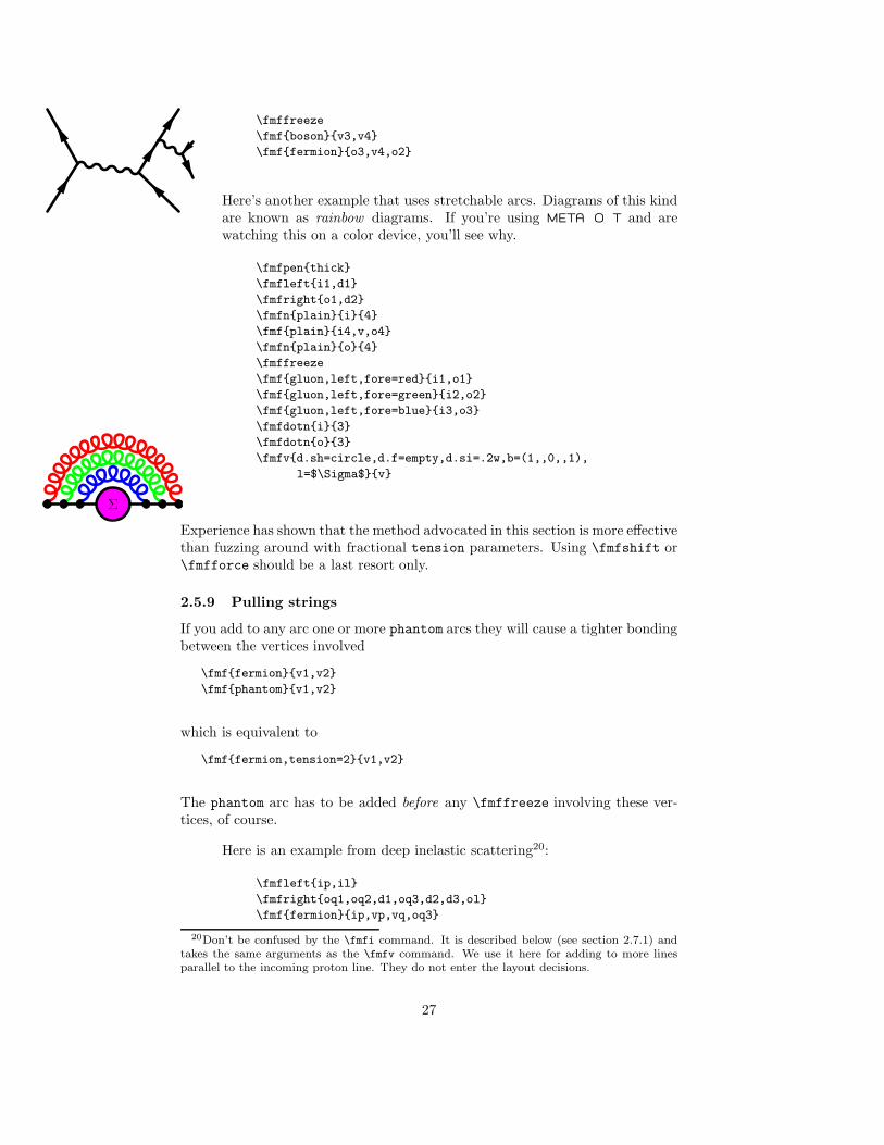
Here’s another example that uses stretchable arcs. Diagrams of this kindare known as rainbow diagrams. If you’re using META O T and arewatching this on a color device, you’ll see why.
\fmfpen{thick}
\fmfleft{i1,d1}
\fmfright{o1,d2}
\fmfn{plain}{i}{4}
\fmf{plain}{i4,v,o4}
\fmfn{plain}{o}{4}
\fmffreeze
\fmf{gluon,left,fore=red}{i1,o1}
\fmf{gluon,left,fore=green}{i2,o2}
\fmf{gluon,left,fore=blue}{i3,o3}
\fmfdotn{i}{3}
\fmfdotn{o}{3}
\fmfv{d.sh=circle,d.f=empty,d.si=.2w,b=(1,,0,,1),
l=$\Sigma$}{v}
Σ
Experience has shown that the method advocated in this section is more effectivethan fuzzing around with fractional tension parameters. Using \fmfshift or\fmfforce should be a last resort only.
2.5.9 Pulling strings
If you add to any arc one or more phantom arcs they will cause a tighter bondingbetween the vertices involved
\fmf{fermion}{v1,v2}
\fmf{phantom}{v1,v2}
which is equivalent to
\fmf{fermion,tension=2}{v1,v2}
The phantom arc has to be added before any \fmffreeze involving these ver-tices, of course.
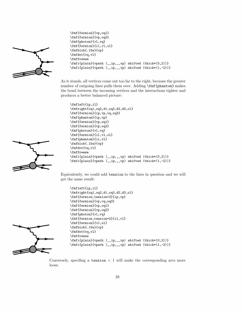
Here is an example from deep inelastic scattering20:
\fmfleft{ip,il}
\fmfright{oq1,oq2,d1,oq3,d2,d3,ol}
\fmf{fermion}{ip,vp,vq,oq3}
20Don’t be confused by the \fmfi command. It is described below (see section 2.7.1) andtakes the same arguments as the \fmfv command. We use it here for adding to more linesparallel to the incoming proton line. They do not enter the layout decisions.
27
\fmf{fermion}{vp,oq1}
\fmf{fermion}{vp,oq2}
\fmf{photon}{vl,vq}
\fmf{fermion}{il,vl,ol}
\fmfblob{.15w}{vp}
\fmfdot{vq,vl}
\fmffreeze
\fmfi{plain}{vpath (__ip,__vp) shifted (thick*(0,2))}
\fmfi{plain}{vpath (__ip,__vp) shifted (thick*(1,-2))}
As it stands, all vertices come out too far to the right, because the greaternumber of outgoing lines pulls them over. Adding \fmf{phantom} makesthe bond between the incoming vertices and the interactions tighter andproduces a better balanced picture:
\fmfleft{ip,il}
\fmfright{oq1,oq2,d1,oq3,d2,d3,ol}
\fmf{fermion}{ip,vp,vq,oq3}
\fmf{phantom}{ip,vp}
\fmf{fermion}{vp,oq1}
\fmf{fermion}{vp,oq2}
\fmf{photon}{vl,vq}
\fmf{fermion}{il,vl,ol}
\fmf{phantom}{il,vl}
\fmfblob{.15w}{vp}
\fmfdot{vq,vl}
\fmffreeze
\fmfi{plain}{vpath (__ip,__vp) shifted (thick*(0,2))}
\fmfi{plain}{vpath (__ip,__vp) shifted (thick*(1,-2))}
Equivalently, we could add tension to the lines in question and we willget the same result:
\fmfleft{ip,il}
\fmfright{oq1,oq2,d1,oq3,d2,d3,ol}
\fmf{fermion,tension=2}{ip,vp}
\fmf{fermion}{vp,vq,oq3}
\fmf{fermion}{vp,oq1}
\fmf{fermion}{vp,oq2}
\fmf{photon}{vl,vq}
\fmf{fermion,tension=2}{il,vl}
\fmf{fermion}{vl,ol}
\fmfblob{.15w}{vp}
\fmfdot{vq,vl}
\fmffreeze
\fmfi{plain}{vpath (__ip,__vp) shifted (thick*(0,2))}
\fmfi{plain}{vpath (__ip,__vp) shifted (thick*(1,-2))}
Conversely, specifing a tension < 1 will make the corresponding arcs moreloose.
28
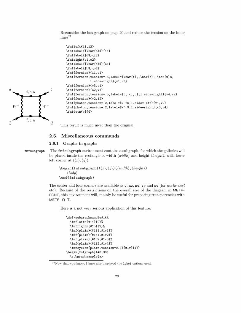
Reconsider the box graph on page 20 and reduce the tension on the innerlines21
\fmfleft{i1,i2}
\fmflabel{$\bar{b}$}{i1}
\fmflabel{$d$}{i2}
\fmfright{o1,o2}
\fmflabel{$\bar{d}$}{o1}
\fmflabel{$b$}{o2}
\fmf{fermion}{i1,v1}
\fmf{fermion,tension=.5,label=$\bar{t},,\bar{c},,\bar{u}$,
l.side=right}{v1,v3}
\fmf{fermion}{v3,o1}
\fmf{fermion}{o2,v4}
\fmf{fermion,tension=.5,label=$t,,c,,u$,l.side=right}{v4,v2}
\fmf{fermion}{v2,i2}
\fmf{photon,tension=.2,label=$W^+$,l.side=left}{v1,v2}
\fmf{photon,tension=.2,label=$W^-$,l.side=right}{v3,v4}
\fmfdotn{v}{4}
t, c, u
W+ W−
t, c, u
b
d
d
b
This result is much nicer than the original.
2.6 Miscellaneous commands
2.6.1 Graphs in graphs
The fmfsubgraph environment contains a subgraph, for which the galleries willfmfsubgraph
be placed inside the rectangle of width 〈width〉 and height 〈height〉, with lowerleft corner at (〈x 〉, 〈y〉):
\begin{fmfsubgraph}(〈x 〉,〈y〉)(〈width〉,〈height〉)〈body〉
\end{fmfsubgraph}
The center and four corners are available as c, nw, ne, sw and se (for north-westetc). Because of the restrictions on the overall size of the diagram in META-FONT, this environment will, mainly be useful for preparing transparencies withMETA O T.
Here is a not very serious application of this feature:
\def\subgraphsample#1{%
\fmfleftn{#1i}{2}%
\fmfrightn{#1o}{2}%
\fmf{plain}{#1i1,#1v1}%
\fmf{plain}{#1o1,#1v2}%
\fmf{plain}{#1o2,#1v3}%
\fmf{plain}{#1i2,#1v4}%
\fmfcyclen{plain,tension=0.3}{#1v}{4}}
\begin{fmfgraph}(40,30)
\subgraphsample{a}
21Now that you know, I have also displayed the label options used.
29
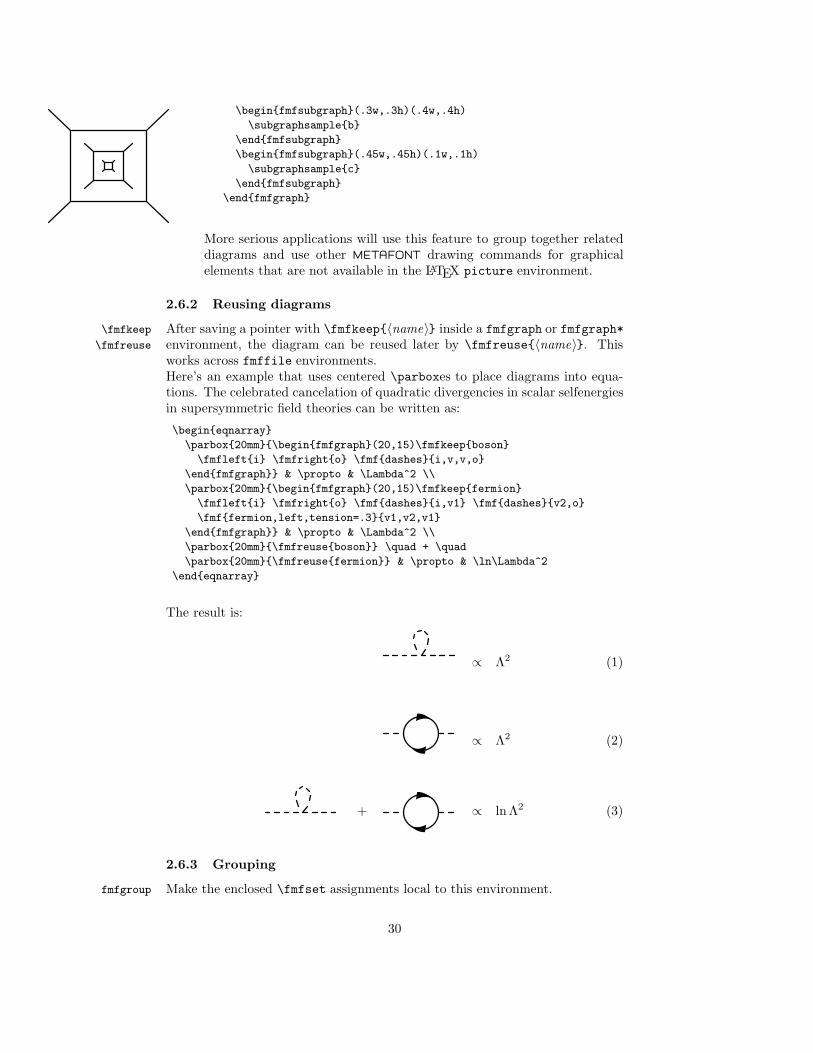
\begin{fmfsubgraph}(.3w,.3h)(.4w,.4h)
\subgraphsample{b}
\end{fmfsubgraph}
\begin{fmfsubgraph}(.45w,.45h)(.1w,.1h)
\subgraphsample{c}
\end{fmfsubgraph}
\end{fmfgraph}
More serious applications will use this feature to group together relateddiagrams and use other METAFONT drawing commands for graphicalelements that are not available in the LATEX picture environment.
2.6.2 Reusing diagrams
After saving a pointer with \fmfkeep{〈name〉} inside a fmfgraph or fmfgraph*\fmfkeep
\fmfreuse environment, the diagram can be reused later by \fmfreuse{〈name〉}. Thisworks across fmffile environments.Here’s an example that uses centered \parboxes to place diagrams into equa-tions. The celebrated cancelation of quadratic divergencies in scalar selfenergiesin supersymmetric field theories can be written as:
\begin{eqnarray}
\parbox{20mm}{\begin{fmfgraph}(20,15)\fmfkeep{boson}
\fmfleft{i} \fmfright{o} \fmf{dashes}{i,v,v,o}
\end{fmfgraph}} & \propto & \Lambda^2 \\
\parbox{20mm}{\begin{fmfgraph}(20,15)\fmfkeep{fermion}
\fmfleft{i} \fmfright{o} \fmf{dashes}{i,v1} \fmf{dashes}{v2,o}
\fmf{fermion,left,tension=.3}{v1,v2,v1}
\end{fmfgraph}} & \propto & \Lambda^2 \\
\parbox{20mm}{\fmfreuse{boson}} \quad + \quad
\parbox{20mm}{\fmfreuse{fermion}} & \propto & \ln\Lambda^2
\end{eqnarray}
The result is:
∝ Λ2 (1)
∝ Λ2 (2)
+ ∝ ln Λ2 (3)
2.6.3 Grouping
Make the enclosed \fmfset assignments local to this environment.fmfgroup
30
Parameter Default Semanticsthin 1pt thin arcsthick 1.5thin thicker arcsarrow_len 4mm length of arrow headarrow_ang 15 opening angle of arrow headcurly_len 3mm length of one curldash_len 3mm length of one dashdot_len 2mm distance of two dotswiggly_len 4mm length of one wigglewiggly_slope 60 inclination of wiggleszigzag_len 2mm length of a zig-zag periodzigzag_width 2thick width of zig-zag linesdecor_size 5mm default size of vertex decorsdot_size 4thick diameter of dots
Table 7: Available style parameters.
2.6.4 Changing parameters
This command can be used to change the parameters in table 7 as follows:\fmfset
\fmfset{〈parameter〉}{〈value〉}
Note that these parameters are not stored in the graph data structure for theindividual vertices and arcs. Instead the current values at the time of \fmfdraware used.
2.6.5 Shrinking
Shrink the linewidths and similar parameters in the enclosed section.fmfshrink
2.6.6 Debugging
Enable and disable tracing of the layout decisions. This is not necessarily\fmftrace
\fmfnotrace printed in an intuitive format, but can be helpful for debugging.Enable online displays. \fmfstopdisplay will halt METAFONT everytime a\fmfdisplay
\fmfstopdisplay graph is complete.
2.6.7 Multiple vertices and arcs
The environmentfmffor
\begin{fmffor}{〈var〉}{〈from〉}{〈step〉}{〈to〉}〈body〉
\end{fmffor}
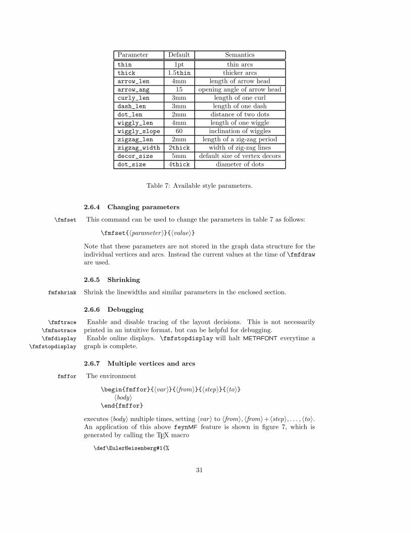
executes 〈body〉 multiple times, setting 〈var〉 to 〈from〉, 〈from〉+〈step〉, . . . , 〈to〉.An application of this above feynMF feature is shown in figure 7, which isgenerated by calling the TEX macro
\def\EulerHeisenberg#1{%
31
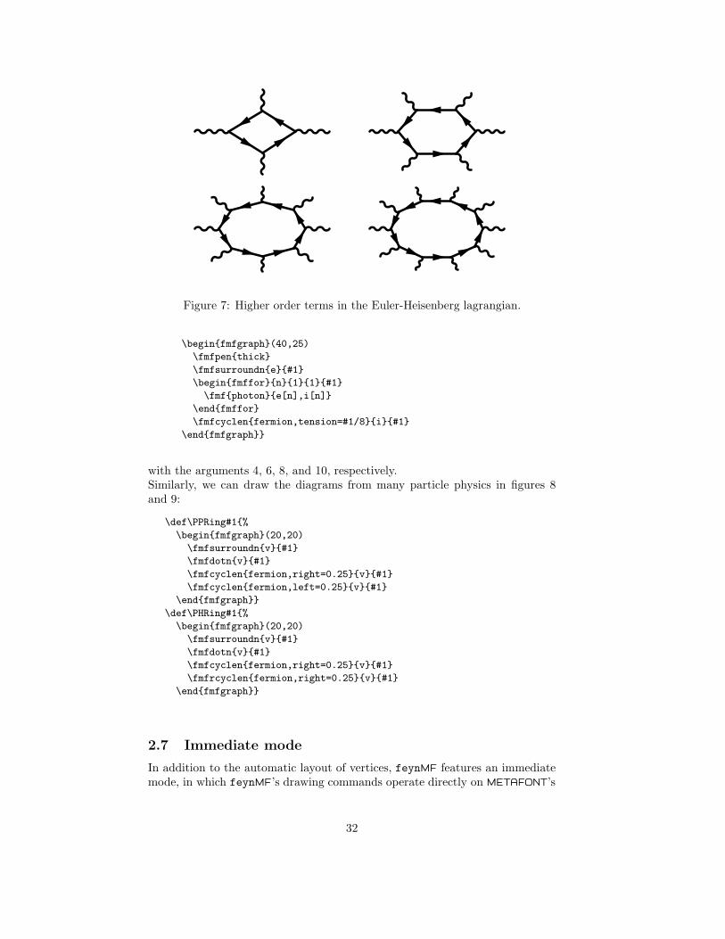
Figure 7: Higher order terms in the Euler-Heisenberg lagrangian.
\begin{fmfgraph}(40,25)
\fmfpen{thick}
\fmfsurroundn{e}{#1}
\begin{fmffor}{n}{1}{1}{#1}
\fmf{photon}{e[n],i[n]}
\end{fmffor}
\fmfcyclen{fermion,tension=#1/8}{i}{#1}
\end{fmfgraph}}
with the arguments 4, 6, 8, and 10, respectively.Similarly, we can draw the diagrams from many particle physics in figures 8and 9:
\def\PPRing#1{%
\begin{fmfgraph}(20,20)
\fmfsurroundn{v}{#1}
\fmfdotn{v}{#1}
\fmfcyclen{fermion,right=0.25}{v}{#1}
\fmfcyclen{fermion,left=0.25}{v}{#1}
\end{fmfgraph}}
\def\PHRing#1{%
\begin{fmfgraph}(20,20)
\fmfsurroundn{v}{#1}
\fmfdotn{v}{#1}
\fmfcyclen{fermion,right=0.25}{v}{#1}
\fmfrcyclen{fermion,right=0.25}{v}{#1}
\end{fmfgraph}}
2.7 Immediate mode
In addition to the automatic layout of vertices, feynMF features an immediatemode, in which feynMF’s drawing commands operate directly on METAFONT’s
32
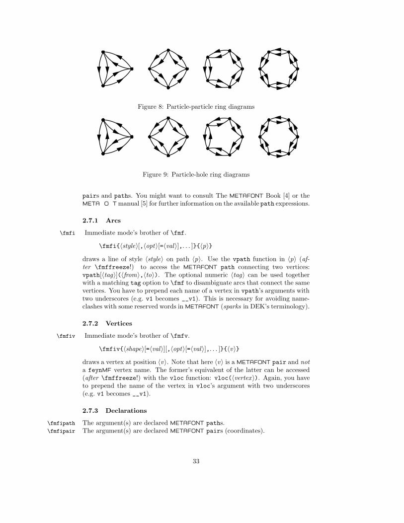
Figure 8: Particle-particle ring diagrams
Figure 9: Particle-hole ring diagrams
pairs and paths. You might want to consult The METAFONT Book [4] or theMETA O T manual [5] for further information on the available path expressions.
2.7.1 Arcs
Immediate mode’s brother of \fmf.\fmfi
\fmfi{〈style〉[,〈opt〉[=〈val〉],. . . ]}{〈p〉}
draws a line of style 〈style〉 on path 〈p〉. Use the vpath function in 〈p〉 (af-ter \fmffreeze!) to access the METAFONT path connecting two vertices:vpath[〈tag〉](〈from〉,〈to〉). The optional numeric 〈tag〉 can be used togetherwith a matching tag option to \fmf to disambiguate arcs that connect the samevertices. You have to prepend each name of a vertex in vpath’s arguments withtwo underscores (e.g. v1 becomes __v1). This is necessary for avoiding name-clashes with some reserved words in METAFONT (sparks in DEK’s terminology).
2.7.2 Vertices
Immediate mode’s brother of \fmfv.\fmfiv
\fmfiv{〈shape〉[=〈val〉][,〈opt〉[=〈val〉],. . . ]}{〈v〉}
draws a vertex at position 〈v〉. Note that here 〈v〉 is a METAFONT pair and nota feynMF vertex name. The former’s equivalent of the latter can be accessed(after \fmffreeze!) with the vloc function: vloc(〈vertex 〉). Again, you haveto prepend the name of the vertex in vloc’s argument with two underscores(e.g. v1 becomes __v1).
2.7.3 Declarations
The argument(s) are declared METAFONT paths.\fmfipath
The argument(s) are declared METAFONT pairs (coordinates).\fmfipair
33
2.7.4 Assignments
Establish equality for the two arguments, i.e. \fmfiequ{lval}{rval} translates\fmfiequ
to lval=rval.Assign the second argument to the first, i.e. \fmfiset{lval}{rval} translates\fmfiset
to lval:=rval.Specifying equality of two variables is a very different operation from assignmentin METAFONT. See The METAFONT Book [4] for details on METAFONT’s builtinequation solver.
2.7.5 Examples
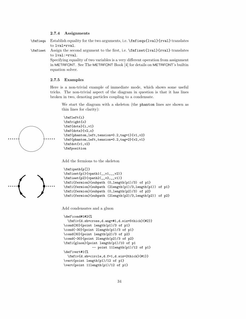
Here is a non-trivial example of immediate mode, which shows some usefultricks. The non-trivial aspect of the diagram in question is that it has linesbroken in two, denoting particles coupling to a condensate.
We start the diagram with a skeleton (the phantom lines are shown asthin lines for clarity):
\fmfleft{i}
\fmfright{o}
\fmf{dots}{i,v1}
\fmf{dots}{v2,o}
\fmf{phantom,left,tension=0.2,tag=1}{v1,v2}
\fmf{phantom,left,tension=0.2,tag=2}{v2,v1}
\fmfdot{v1,v2}
\fmfposition
Add the fermions to the skeleton
\fmfipath{p[]}
\fmfiset{p1}{vpath1(__v1,__v2)}
\fmfiset{p2}{vpath2(__v2,__v1)}
\fmfi{fermion}{subpath (0,length(p1)/3) of p1}
\fmfi{fermion}{subpath (2length(p1)/3,length(p1)) of p1}
\fmfi{fermion}{subpath (0,length(p2)/3) of p2}
\fmfi{fermion}{subpath (2length(p2)/3,length(p2)) of p2}
Add condensates and a gluon
\def\cond#1#2{%
\fmfiv{d.sh=cross,d.ang=#1,d.siz=5thick}{#2}}
\cond{30}{point length(p1)/3 of p1}
\cond{-30}{point 2length(p1)/3 of p1}
\cond{30}{point length(p2)/3 of p2}
\cond{-30}{point 2length(p2)/3 of p2}
\fmfi{gluon}{point length(p1)/10 of p1
-- point 11length(p1)/12 of p1}
\def\vert#1{%
\fmfiv{d.sh=circle,d.f=1,d.siz=2thick}{#1}}
\vert{point length(p1)/12 of p1}
\vert{point 11length(p1)/12 of p1}
34
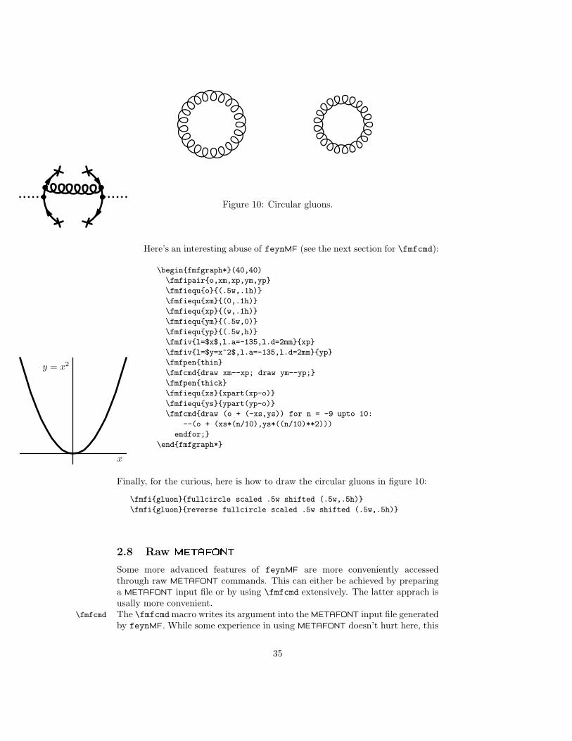
Figure 10: Circular gluons.
Here’s an interesting abuse of feynMF (see the next section for \fmfcmd):
\begin{fmfgraph*}(40,40)
\fmfipair{o,xm,xp,ym,yp}
\fmfiequ{o}{(.5w,.1h)}
\fmfiequ{xm}{(0,.1h)}
\fmfiequ{xp}{(w,.1h)}
\fmfiequ{ym}{(.5w,0)}
\fmfiequ{yp}{(.5w,h)}
\fmfiv{l=$x$,l.a=-135,l.d=2mm}{xp}
\fmfiv{l=$y=x^2$,l.a=-135,l.d=2mm}{yp}
\fmfpen{thin}
\fmfcmd{draw xm--xp; draw ym--yp;}
\fmfpen{thick}
\fmfiequ{xs}{xpart(xp-o)}
\fmfiequ{ys}{ypart(yp-o)}
\fmfcmd{draw (o + (-xs,ys)) for n = -9 upto 10:
--(o + (xs*(n/10),ys*((n/10)**2)))
endfor;}
\end{fmfgraph*}
x
y = x2
Finally, for the curious, here is how to draw the circular gluons in figure 10:
\fmfi{gluon}{fullcircle scaled .5w shifted (.5w,.5h)}
\fmfi{gluon}{reverse fullcircle scaled .5w shifted (.5w,.5h)}
2.8 Raw METAFONT
Some more advanced features of feynMF are more conveniently accessedthrough raw METAFONT commands. This can either be achieved by preparinga METAFONT input file or by using \fmfcmd extensively. The latter apprach isusally more convenient.The \fmfcmdmacro writes its argument into the METAFONT input file generated\fmfcmd
by feynMF. While some experience in using METAFONT doesn’t hurt here, this
35
approach can simplify the production of complex diagrams considerably. Notethat no semicolon is appended, the user has to provide it explicitely.
2.8.1 Extending feynMF
A prominent example for using raw METAFONT is provided by the option to addnew styles for arcs. There is of course always one more style that must be addedto the default list. But increasing this list without bounds will eventually slowdown feynMF and increase its memory requirements. It is therefore better toallow users to define their own styles. This is done with the METAFONT macrostyle_def, which defines a macro that will be called to do the drawing andregisters this macro with feynMF so that it can be used in the first argumentto \fmf.The macro takes one argument of type path and is responsible for drawing thearc on this path. If META O T’s color functionality is to be used, the coloraware functions cdraw, cfill, cfilldraw, ccutdraw and cdrawdot should beused instead of draw, etc.
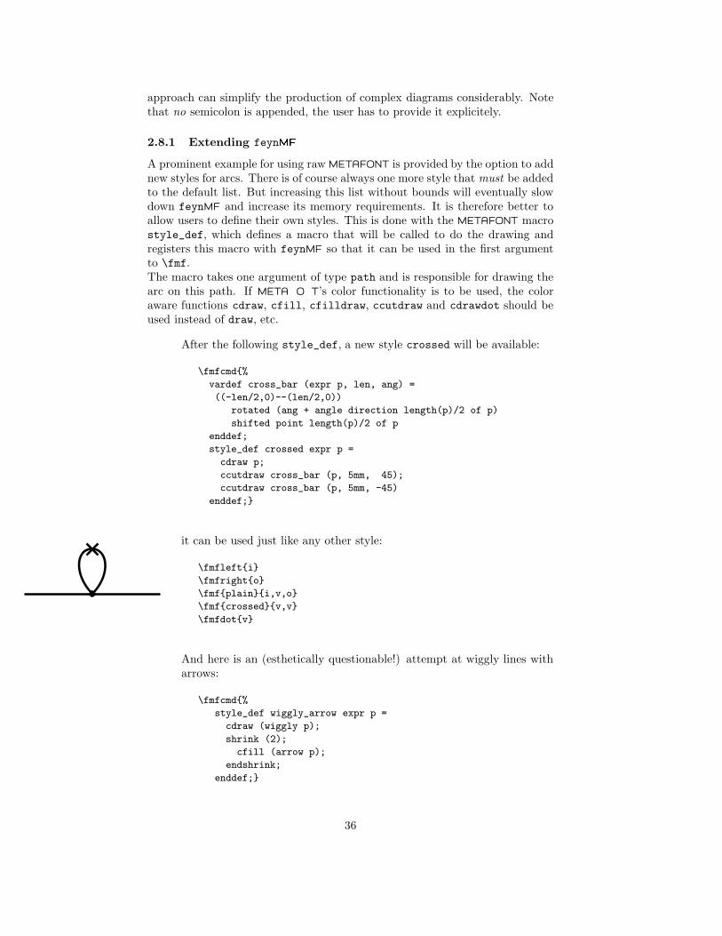
After the following style_def, a new style crossed will be available:
\fmfcmd{%
vardef cross_bar (expr p, len, ang) =
((-len/2,0)--(len/2,0))
rotated (ang + angle direction length(p)/2 of p)
shifted point length(p)/2 of p
enddef;
style_def crossed expr p =
cdraw p;
ccutdraw cross_bar (p, 5mm, 45);
ccutdraw cross_bar (p, 5mm, -45)
enddef;}
it can be used just like any other style:
\fmfleft{i}
\fmfright{o}
\fmf{plain}{i,v,o}
\fmf{crossed}{v,v}
\fmfdot{v}
And here is an (esthetically questionable!) attempt at wiggly lines witharrows:
\fmfcmd{%
style_def wiggly_arrow expr p =
cdraw (wiggly p);
shrink (2);
cfill (arrow p);
endshrink;
enddef;}
36
Note how the shrink macro (which is the METAFONT equivalent of thefmfshrink environment) is used to temporarily double the dimensions ofthe arrowhead which is constructed by the arrow macro.
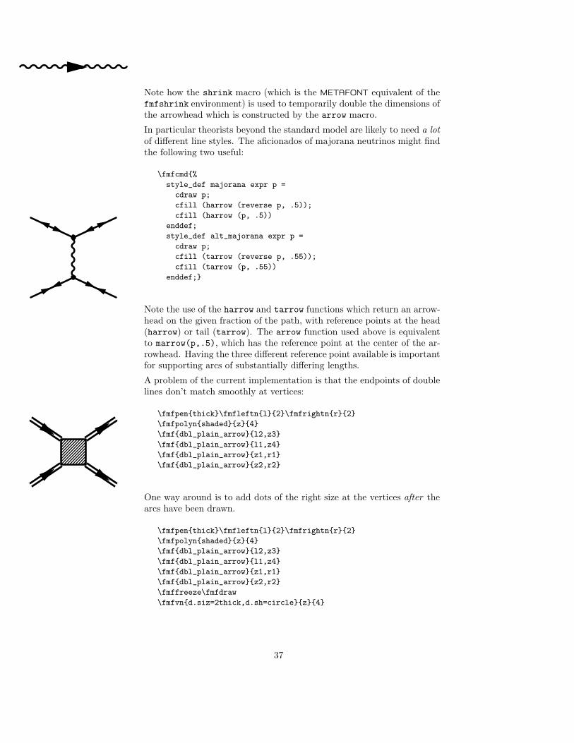
In particular theorists beyond the standard model are likely to need a lotof different line styles. The aficionados of majorana neutrinos might findthe following two useful:
\fmfcmd{%
style_def majorana expr p =
cdraw p;
cfill (harrow (reverse p, .5));
cfill (harrow (p, .5))
enddef;
style_def alt_majorana expr p =
cdraw p;
cfill (tarrow (reverse p, .55));
cfill (tarrow (p, .55))
enddef;}
Note the use of the harrow and tarrow functions which return an arrow-head on the given fraction of the path, with reference points at the head(harrow) or tail (tarrow). The arrow function used above is equivalentto marrow(p,.5), which has the reference point at the center of the ar-rowhead. Having the three different reference point available is importantfor supporting arcs of substantially differing lengths.
A problem of the current implementation is that the endpoints of doublelines don’t match smoothly at vertices:
\fmfpen{thick}\fmfleftn{l}{2}\fmfrightn{r}{2}
\fmfpolyn{shaded}{z}{4}
\fmf{dbl_plain_arrow}{l2,z3}
\fmf{dbl_plain_arrow}{l1,z4}
\fmf{dbl_plain_arrow}{z1,r1}
\fmf{dbl_plain_arrow}{z2,r2}
One way around is to add dots of the right size at the vertices after thearcs have been drawn.
\fmfpen{thick}\fmfleftn{l}{2}\fmfrightn{r}{2}
\fmfpolyn{shaded}{z}{4}
\fmf{dbl_plain_arrow}{l2,z3}
\fmf{dbl_plain_arrow}{l1,z4}
\fmf{dbl_plain_arrow}{z1,r1}
\fmf{dbl_plain_arrow}{z2,r2}
\fmffreeze\fmfdraw
\fmfvn{d.siz=2thick,d.sh=circle}{z}{4}
37
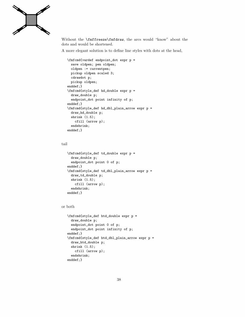
Without the \fmffreeze\fmfdraw, the arcs would “know” about thedots and would be shortened.
A more elegant solution is to define line styles with dots at the head,
\fmfcmd{vardef endpoint_dot expr p =
save oldpen; pen oldpen;
oldpen := currentpen;
pickup oldpen scaled 3;
cdrawdot p;
pickup oldpen;
enddef;}
\fmfcmd{style_def hd_double expr p =
draw_double p;
endpoint_dot point infinity of p;
enddef;}
\fmfcmd{style_def hd_dbl_plain_arrow expr p =
draw_hd_double p;
shrink (1.5);
cfill (arrow p);
endshrink;
enddef;}
tail
\fmfcmd{style_def td_double expr p =
draw_double p;
endpoint_dot point 0 of p;
enddef;}
\fmfcmd{style_def td_dbl_plain_arrow expr p =
draw_td_double p;
shrink (1.5);
cfill (arrow p);
endshrink;
enddef;}
or both
\fmfcmd{style_def htd_double expr p =
draw_double p;
endpoint_dot point 0 of p;
endpoint_dot point infinity of p;
enddef;}
\fmfcmd{style_def htd_dbl_plain_arrow expr p =
draw_htd_double p;
shrink (1.5);
cfill (arrow p);
endshrink;
enddef;}
38
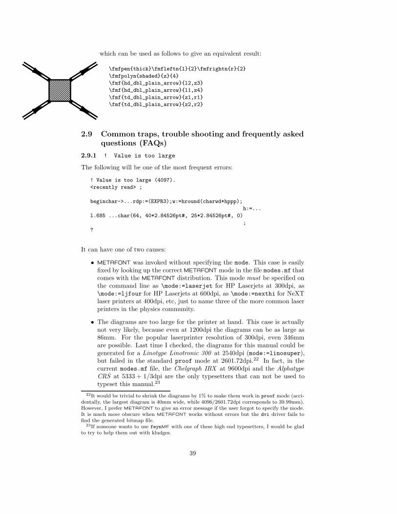
which can be used as follows to give an equivalent result:
\fmfpen{thick}\fmfleftn{l}{2}\fmfrightn{r}{2}
\fmfpolyn{shaded}{z}{4}
\fmf{hd_dbl_plain_arrow}{l2,z3}
\fmf{hd_dbl_plain_arrow}{l1,z4}
\fmf{td_dbl_plain_arrow}{z1,r1}
\fmf{td_dbl_plain_arrow}{z2,r2}
2.9 Common traps, trouble shooting and frequently askedquestions (FAQs)
2.9.1 ! Value is too large
The following will be one of the most frequent errors:
! Value is too large (4097).
<recently read> ;
beginchar->...rdp:=(EXPR3);w:=hround(charwd*hppp);
h:=...
l.685 ...char(64, 40*2.84526pt#, 25*2.84526pt#, 0)
;
?
It can have one of two causes:
• METAFONT was invoked without specifying the mode. This case is easilyfixed by looking up the correct METAFONT mode in the file modes.mf thatcomes with the METAFONT distribution. This mode must be specified onthe command line as \mode:=laserjet for HP Laserjets at 300dpi, as\mode:=ljfour for HP Laserjets at 600dpi, as \mode:=nexthi for NeXTlaser printers at 400dpi, etc, just to name three of the more common laserprinters in the physics community.
• The diagrams are too large for the printer at hand. This case is actuallynot very likely, because even at 1200dpi the diagrams can be as large as86mm. For the popular laserprinter resolution of 300dpi, even 346mmare possible. Last time I checked, the diagrams for this manual could begenerated for a Linotype Linotronic 300 at 2540dpi (mode:=linosuper),but failed in the standard proof mode at 2601.72dpi.22 In fact, in thecurrent modes.mf file, the Chelgraph IBX at 9600dpi and the AlphatypeCRS at 5333 + 1/3dpi are the only typesetters that can not be used totypeset this manual.23
22It would be trivial to shrink the diagrams by 1% to make them work in proof mode (acci-dentally, the largest diagram is 40mm wide, while 4096/2601.72dpi corresponds to 39.99mm).However, I prefer METAFONT to give an error message if the user forgot to specify the mode.It is much more obscure when METAFONT works without errors but the dvi driver fails tofind the generated bitmap file.
23If someone wants to use feynMF with one of these high end typesetters, I would be gladto try to help them out with kludges.
39
2.9.2 Diagrams in the document are never updated
There are two known reasons why diagrams may not be updated the documentafter the source file has been changed:
• Some dvi file previewers (e.g. xdvi(1) under UNIX) do not reread fontinformation if the tfm or pk files have changed, even though they rereadthe dvi file if it has changed. Therefore you have to restart such previewersif you have made changes in diagrams to see these changes on the screen.
• Some dvi drivers (e.g. dvips(1) under UNIX) do not work with the gffiles directly, but convert them with an external program to pk formatfirst. On later occasions, the dvi driver will then use the pk file which isout of date with respect to the sources and the gf file. The only knownfix is to delete the pk fils before running the dvi driver.
2.9.3 Disgrams show up in the wrong spot
If you are using feynMF with LATEX’s \includeonly feature, you should watchout for the following situation:
\includeonly{bar1,bar3}
\begin{fmffile}{foograph}
\include{bar1}
\include{bar2}
\include{bar3}
\end{fmffile}
where bar1.tex defines graph #1, bar2.tex graph #2 and bar3.tex definesgraph #3. If you now proceeded to add graphs to bar1.tex, you will noticethat a second graph is accepted, but instead of the new third graph, the oldgraph #3 appears. What happens is that LATEX stores the value of the counterfor fmfgraphs in each .aux file so that because bar2.tex is not processed, thiscounter is always reset to 3 at the beginning of bar3.tex.Even though this situation appears to be contrived, it actually occured in reallife applications and the resulting error is very confusing.The only “fix” for this problem would be to use a private counter behind LATEX’sback. Unfortunately, it appears that this will violate the principle of minimalsurprise even more. It is therefore usually a good idea to reprocess the completedocument when the number of graphs has changed in an \included file. Theother solution is to have a separate fmfgraph environment for each \includedfile.
2.9.4 Spurious labels show up
If spurious labels show up in your diagrams, this is most likely caused by oldlabel files (e.g. foo.t〈n〉) still lying around. Just delete these files and rerunTEX and METAFONT (or META O T respectively).
40

2.10 Known bugs
2.10.1 Chaotic manual
This is being worked on. It should probably be rewritten from scratch, but Idon’t have enough time at the moment (this is a spare time activity).
2.10.2 Delayed error messages
This can’t be fixed. The problem is that errors can manifest themselves only along time after the corresponding source line has been read. Since TEX doesn’tallow to access the current source line number, there is no way to store thisinformation along with the other information on the graph. I can only hope tohave enough sanity checks in place some day that error messages from META-FONT won’t occur.
2.10.3 Multiple tadpoles
Currently, feynMF will not layout multiple tadpoles at a single vertex auto-matically. This could be fixed in principle, but these fixes would cause otherproblems which are more inconvenient than having to lay out tadpoles manually.
2.10.4 Hard limits
Currently the most severe limitation lies in the size of the generated pictures.The largest number METAFONT can represent internally is 4095.99998 and thisis also the largest value any coordinate measured in pixels can assume. Atthe most popular laserprinter resolution of 300 dots per inch (dpi), this corre-sponds to a horizontal and vertical extension of about 346mm, which is plentyand we’re more likely to hit the internal limits on the complexity of a picture.However, at the proof mode resolution of 2601.72dpi, this is reduced to slightlyless than 40mm and we’re running the risk of arithmetic overflow in internalcalculations much earlier.There are two potential solutions of different scope and complexity:
• Since John Hobby’s META O T is now available without a non-disclosureagreement from AT&T, one solution is to replace METAFONT by META-
O T, which doesn’t suffer from the size limitations. This comes witha small price paid in reduced portability of the generated output, but asalready stated above in the case of axodraw, the ubiquity of PostScriptprinters (and the free GhostScript interpreter) makes this a minor point.
• The more ambitious solutions would be virtual graphs, i.e. graphs whichare larger than the current limit enforced by numeric overflow at higherresolutions. This could be implemented by calculating the layout of aminiature graph and afterwards distributing the full graph among severalMETAFONT characters.
Acknowledgements
I am most grateful to Wolfgang Kilian, who pushed feynMF’s predecessorfeynman.mf to its limits [12]. Discussions with him triggered a lot of good
41
ideas. Thanks also to my students and the people on The Net for suggestions,portability fixes and for volunteering as guinea pigs.
References
[1] Donald E. Knuth, The TEXbook, Addison-Wesley, Reading MA, 1986.
[2] Leslie Lamport, LATEX — A Documentation Preparation System, Addison-Wesley, Reading MA, 1985.
[3] Michel Goosens, Frank Mittelbach, and Alexander Samarin, The LATEXCompanion, Addison-Wesley, Reading MA, 1994.
[4] Donald E. Knuth, The METAFONTbook, Addison-Wesley, Reading MA,1986.
[5] John D. Hobby, A User’s Manual for META O T, Computer Science Re-port #162, AT&T Bell Laboratories, April 1992.
[6] Thorsten Ohl, Comp. Phys. Comm. 90 (1995) 340.
[7] Thorsten Ohl, CERN Computer Newsletter 220 (1995) 22; 221 (1995) 46;222 (1996) 24.
[8] Micheal J. S. Levine, Comp. Phys. Comm. 58 (1990) 181.
[9] Jos Vermaseren, Comp. Phys. Comm. 83 (1994) 45. axodraw is availablefrom CTAN (cf. p. 42), in the graphics directory.
[10] Thomas E. Leathrum, mfpic, available from CTAN (cf. p. 42), in thegraphics directory.
[11] Tim Stelzer and Bill Long, Comp. Phys. Comm. 81 (1994) 357.
[12] Wolfgang Kilian, Doctoral Thesis, Technical University Darmstadt, 1994.
[13] Alan Jeffrey, Lists in TEX’s Mouth, TUGboat 199?.
Distribution
feynMF is available by anonymous internet ftp from any of the ComprehensiveTEX Archive Network (CTAN) hosts
ftp.shsu.edu, ftp.tex.ac.uk, ttp.dante.de
in the directory
macros/latex/contrib/supported/feynmf
It is also available from the host
crunch.ikp.physik.th-darmstadt.de
in the directory
42
pub/ohl/feynmf
Unsupported snapshots of my work in progress are provided as
pub/ohl/feynmf.versions/feynmf-current.tar.gz
There are two mailing lists
[email protected]@crunch.ikp.physik.th-darmstadt.de
open for subscription. The former should carry only important announcements,of new versions in particular. To subscribe, send mail to the (electronic) mailinglist manager
and not to the lists itself. The following commands (on a line in the body ofthe mail, not in the subject) are useful:
subscribe feynmf-announceunsubscribe feynmf-announcehelp
Index
Numbers written in italic refer to the page where the corresponding entry isdescribed, the ones underlined to the code line of the definition, the rest to thecode lines where the entry is used.
-T, --notfm, 13-c, --clean, 13-f, --force, 13-h, --help, 12-m mode, --mode
mode, 13-n, --noexec, 13-q, --quiet, 13-t, --tfm tfm, 13-v, --version, 12
arcs=arcs, 14, 16, 33
blobs=blobs, 17
color=color, 19crossed arcs=crossed
arcs, 36
defining newstyles=definingnew styles, 36
displays, on-line=displays,online, 31
dots=dots, 17
environments:¿fmffile,8
environments:¿fmffor, 31environments:¿fmfgraph*,
9environments:¿fmfgraph,
9environments:¿fmfgroup,
30environments:¿fmfshrink,
31environments:¿fmfsubgraph,
29extensions=extensions, 36external ver-
tices=externalvertices, 14
file, 13file ..., 13fmf= \subitem *+\fmf+, \usage{14}
fmfblob= \subitem *+\fmfblob+, \usage{17}
fmfblobn= \subitem *+\fmfblobn+, \usage{17}
fmfbottom= \subitem *+\fmfbottom+, \usage{14}
fmfbottomn= \subitem *+\fmfbottomn+, \usage{14}
fmfcmd= \subitem *+\fmfcmd+, \usage{35}
fmfcurved= \subitem *+\fmfcurved+, \usage{14}
fmfcyclen= \subitem *+\fmfcyclen+, \usage{16}
fmfdisplay= \subitem *+\fmfdisplay+, \usage{31}
fmfdot= \subitem *+\fmfdot+, \usage{17}
fmfdotn= \subitem *+\fmfdotn+, \usage{17}
fmffile=fmffile (en-vironment), 8
fmffixed= \subitem *+\fmffixed+, \usage{24}
fmffixedx= \subitem *+\fmffixedx+, \usage{25}
fmffixedy= \subitem *+\fmffixedy+, \usage{25}
fmffor=fmffor (en-vironment), 31
fmfforce= \subitem *+\fmfforce+, \usage{24}
fmfframe= \subitem *+\fmfframe+, \usage{9}
fmffreeze= \subitem *+\fmffreeze+, \usage{24}
fmfgraph*=fmfgraph*
(environment), 9
fmfgraph=fmfgraph
(environment), 9
43
fmfgroup=fmfgroup
(environment), 30fmfi= \subitem *+\fmfi+, \usage{33}
fmfiequ= \subitem *+\fmfiequ+, \usage{34}
fmfipair= \subitem *+\fmfipair+, \usage{33}
fmfipath= \subitem *+\fmfipath+, \usage{33}
fmfiset= \subitem *+\fmfiset+, \usage{34}
fmfiv= \subitem *+\fmfiv+, \usage{33}
fmfkeep= \subitem *+\fmfkeep+, \usage{30}
fmflabel= \subitem *+\fmflabel+, \usage{23}
fmfleft= \subitem *+\fmfleft+, \usage{14}
fmfleftn= \subitem *+\fmfleftn+, \usage{14}
fmfn= \subitem *+\fmfn+, \usage{16}
fmfnotrace= \subitem *+\fmfnotrace+, \usage{31}
fmfpen= \subitem *+\fmfpen+, \usage{16}
fmfpoly= \subitem *+\fmfpoly+, \usage{18}
fmfpolyn= \subitem *+\fmfpolyn+, \usage{18}
fmfrcyclen= \subitem *+\fmfrcyclen+, \usage{16}
fmfreuse= \subitem *+\fmfreuse+, \usage{30}
fmfright= \subitem *+\fmfright+, \usage{14}
fmfrightn= \subitem *+\fmfrightn+, \usage{14}
fmfrpolyn= \subitem *+\fmfrpolyn+, \usage{18}
fmfset= \subitem *+\fmfset+, \usage{31}
fmfshift= \subitem *+\fmfshift+, \usage{24}
fmfshrink=fmfshrink
(environment), 31fmfstopdisplay= \subitem *+\fmfstopdisplay+, \usage{31}
fmfstraight= \subitem *+\fmfstraight+, \usage{14}
fmfsubgraph=fmfsubgraph
(environment), 29fmfsurround= \subitem *+\fmfsurround+, \usage{14}
fmfsurroundn= \subitem *+\fmfsurroundn+, \usage{14}
fmftop= \subitem *+\fmftop+, \usage{14}
fmftopn= \subitem *+\fmftopn+, \usage{14}
fmftrace= \subitem *+\fmftrace+, \usage{31}
fmfv= \subitem *+\fmfv+, \usage{16}
fmfvn= \subitem *+\fmfvn+, \usage{17}
galleries=galleries, 14
internal ver-tices=internalvertices, 16, 17
labels=labels, 14,16, 23, 24
looping=looping, 31
online displays=onlinedisplays, 31
OPTIONS, 12
parameters=parameters,31
polygons=polygons, 18
styles, definingnew=styles,defining new, 36
subgraphs=subgraphs, 29
tadpoles=tadpoles, 22
tracing=tracing, 31
vertices, exter-nal=vertices,external, 14
vertices, inter-nal=vertices,internal, 16, 17
vertices=vertices, 33
44


![feynMF Drawing Feynman Diagrams with LTEX and METAFONTmirror.las.iastate.edu/tex-archive/macros/latex/contrib/feynmf/fmfman.p… · METAFONT4 [4] and METAPOST5 [5] appear to be the](https://static.fdocuments.net/doc/165x107/606dbf35d306c022274addd3/feynmf-drawing-feynman-diagrams-with-ltex-and-metafont4-4-and-metapost5-5-appear.jpg)


