DIGITAL OUTCROP MAPPING OF A RESERVOIR-SCALE INCISED VALLEY FILL,

SEGO SANDSTONE, BOOK CLIFFS, UTAH

A Thesis

by

MATTHEW F. FEY

Submitted to the Office of Graduate Studies of Texas A&M University

in partial fulfillment of the requirements for the degree of

MASTER OF SCIENCE

August 2006

Major Subject: Geology

DIGITAL OUTCROP MAPPING OF A RESERVOIR-SCALE INCISED VALLEY FILL,

SEGO SANDSTONE, BOOK CLIFFS, UTAH

A Thesis

by

MATTHEW F. FEY

Submitted to the Office of Graduate Studies of Texas A&M University

in partial fulfillment of the requirements for the degree of

MASTER OF SCIENCE

Approved by:

Chair of Committee, Brian Willis Committee Members, Steven Dorobek William Bryant Head of Department, Richard Carlson

August 2006

Major Subject: Geology

iii

ABSTRACT

Digital Outcrop Mapping of a Reservoir-scale Incised Valley Fill, Sego Sandstone,

Book Cliffs, Utah. (August 2006)

Matthew F. Fey, B.S., State University of New York at New Paltz

Chair of Advisory Committee: Dr. Brian Willis

Outcrop analog studies have long been used to define subsurface correlation

strategies and improve predictions of reservoir heterogeneities that can complicate

production behavior. Recent advancements in geographic information software, 3D

geologic modeling techniques, and survey equipment have the potential to revolutionize

outcrop analog studies. A workflow is developed to create digital outcrop models using a

reflectorless total station, a digital camera, Erdas Photogrammetry Module™, and

Gocad™ to document complex stratal variations across kilometers-long outcrops.

Combining outcrop digital elevation models with orthorectified photographs and detailed

sedimentologic logs provides a framework for static 3D reservoir analog models.

Developed methodologies are demonstrated by mapping rock variations and stratal

geometries within several kilometers-long, sub-parallel exposures of the Lower Sego

Sandstone in San Arroyo Canyon, Book Cliffs, Utah.

The digital outcrop model of the Lower Sego Sandstone documents complex bedding

geometry and facies distribution within two sharp-based sandstone layers. A mapping of

allostratigraphic surfaces through the digital outcrop model provided a framework in

which to analyze facies variations. These surfaces included: 1) Basal erosion surfaces of

iv

these layers interpreted to have formed by tidal erosion of the sea floor during shoreline

regression; 2) a high relief erosion surface within the upper layer interpreted to have

formed during lowstand fluvial incision; and 3) top contacts of layers defined by abrupt

fining to marine shale, which are interpreted to record marine ravinement during

transgression. Facies variations within the lower layer include low sinuosity distributary

channel deposits incised into highly marine bioturbated sandstone. Deposits above the

high-relief erosion surface within the upper layer are a classic valley fill succession,

which processes upward from lowstand fluvial channel deposits, to heterolithic estuarine

deposits, and finally to sandy landward-dipping beds of an estuarine mouth shoal deposit.

The digital outcrop model allows surfaces and facies observation to be mapped within a

structured 3D coordinate system to define reservoir analog models.

v

TABLE OF CONTENTS

Page

ABSTRACT....................................................................................................................... iii

TABLE OF CONTENTS.....................................................................................................v

LIST OF TABLES............................................................................................................ vii

LIST OF FIGURES ......................................................................................................... viii

INTRODUCTION ...............................................................................................................1

DIGITAL OUTCROP MODELS ........................................................................................3

Photogrammetry...............................................................................................................6

Close-range outcrop photogrammetry with Leica Geosystems Suite™......................9

Digital Outcrop Models for Geologic Mapping.............................................................19

Accuracy of Digital Outcrop Models.............................................................................22

Surveying control points along an extensive outcrop................................................22

Camera optical distortion...........................................................................................24

Photogrammetric triangulation and automatic tie point generation...........................26

Surface fitting, orthorectification, and image mosaics ..............................................33

APPLICATION OF DIGITAL OUTCROP MAPPING ...................................................37

Sego Depositional Models .............................................................................................38

Study Area and Methods................................................................................................43

Depositional Interpretations of the Lower Sego Sandstone...........................................51

CONCLUSIONS................................................................................................................64

APPENDIX 1.....................................................................................................................67

APPENDIX 2.....................................................................................................................68

vi

Page

REFERENCES ..................................................................................................................69

VITA..................................................................................................................................71

vii

LIST OF TABLES

Page

Table 1. Test case nomenclature........................................................................................28

Table 2. Test case statistical analysis.................................................................................31

Table 3. Statistical analysis of DOM errors in meters .......................................................35

viii

LIST OF FIGURES

Page

Fig. 1.─ Digital elevation model................................................................................5

Fig. 2. ─ Digital outcrop model. .................................................................................6

Fig. 3.─ Transformation of control point coordinates for use in the LPS suite ............................................................................................................11

Fig. 4.─ Camera positioning diagram......................................................................12

Fig. 5. ─ Point measurement dialog box Within Erdas’ LPS ...................................15

Fig. 6.─ DEM point clouds ......................................................................................17

Fig. 7.─ 3D surfaces.................................................................................................20

Fig. 8.─ Triangulation accuracy test photographs. ..................................................25

Fig. 9.─ Map view of three test cases showing position and number of control and tie points..................................................................................29

Fig. 10.─ Test case accuracy bar graphs....................................................................32

Fig. 11.─ Erroneous DOM.........................................................................................36

Fig. 12.─ Stratigraphy and time scale of the Mesaverde Group in the Book Cliffs of eastern Utah (from A. Willis, 2000, after Fouch et al., 1983 and Obradovich, 1993)......................................................................38

Fig. 13.─ Regional cross section of deposits exposed in the Book Cliffs from Price, Utah, to Grand Junction, Colorado (Modified from Willis and Gabel, 2001)........................................................................................40

ix

Page

Fig. 14.─ Cross-section of the Sego Member showing Van Wagoner’s interpretations of relationships between tidal sandstones and offshore marine deposits (from Willis and Gabel, 2001; after Van Wagoner, 1991)..........................................................................................41

Fig. 15.─ Cross section of the lower Sego Member interval along the southern Book Cliffs outcrop belt. ( Willis and Gabel, 2003). ..................41

Fig. 16.─ Study area location.....................................................................................45

Fig. 17.─ USGS topographic map of the study area..................................................46

Fig. 18.─ Sedimentological logs, datumed on the middle Lower Sego Shale, show lithology, relative amount of bioturbation and paleocurrent in their measured position (see locations in Fig. 3 and key to symbols in Fig. 19)...................................................................................................47

Fig. 19.─ Bedding diagram constructed by tracing of surfaces and facies variations in the field between sedimentological logs. ..............................48

Fig. 20.─ Isopach map of lower sandstone layer .......................................................55

Fig. 21.─ Channel erosion of the middle Lower Sego Shale observed along the middle of the Northern Side Canyon (see Fig. 4..................................58

Fig. 22.─ Lower Sego channels observed in West Wall............................................59

Fig. 23.─ Interpretational lines ..................................................................................60

Fig. 24.─ Channel surface erosion into the middle Lower Sego Shale .....................61

Fig. 25.─ Isopach maps of sequence boundary..........................................................62

1

INTRODUCTION

Outcrop analog studies have long been used to develop subsurface correlation

strategies and to improve predictions of reservoir heterogeneities that can complicate

production behavior. Rock heterogeneities observed in outcrops commonly occur at a

wide variety of scales: (1) core-scale changes in lithofacies that influence local

permeability: (2) interwell-scale variations that complicate local flow patterns; and (3)

field-scale variations that define reservoir compartments. Analog outcrop studies are time

consuming because it is laborious to define and document the character of these diverse

scales within an integrated framework, and it can be difficult to predict in advance which

types and scales of variability will have significant impacts on reservoir behavior. In most

cases reservoir analog studies have consisted of 2D cross sections based on outcrop

photomosaics or the tracing of stratal surfaces between vertical sedimentologic logs.

While these records have proved insightful, more quantitative predictions of

heterogeneity affects on reservoir performance require documentation of rock property

variations in three dimensions; preferably in gridded formats that can be used in dynamic

models of subsurface flow.

Recent advancements in geographic information software, 3D geologic modeling

techniques and survey equipment have the potential to revolutionize outcrop analog

studies; by speeding data acquisition, allowing more accurate documentation of rock

property variations within a complex hierarchy of strata, and providing data formats and

methodologies to accurately define the 3D coordinates of outcrop observations.

___________ This thesis follows the style of Journal of Sedimentary Research.

2

Although there has been a flurry of recent research activity aimed at applying these

new technologies to outcrop reservoir analog studies, most studies completed to date

have focused on developing 3D visualizations of outcrops, rather than on documenting

the 3D geometry of strata and quantifying their internal rock property variations. More

work is required to develop efficient workflows for data acquisition and processing and

to use new types of spatially-oriented outcrop records to improve 3D reservoir modeling.

This study develops a workflow for using a digital camera, a reflectorless laser total

station, Leica Geosystems™ GIS and Mapping suite software (LPS), and Earth

Decision’s Gocad™ geospatial modeling software to document complex stratal variations

across kilometers-long outcrops. Optimization of data collection procedures and accuracy

are examined using controlled studies of a building on the Texas A&M campus. The

utility of these techniques are then demonstrated by the mapping of strata exposed in

several sub-parallel, kilometers-long outcrops of the Sego Sandstone in Utah. These

outcrops were photographed with a digital camera. Digital elevation models of these

outcrops are constructed using surveyed control points and photogrammetry techniques.

The elevation models are used to project photographs into orthorectified photomontages.

Digital elevation models and orthorectified photomontages were combined within

Gocad™ to construct digital outcrop models that are used as 3D base maps to define the

geometry of key stratigraphic surfaces and the positions of measured sedimentologic

logs. The results demonstrate that 3D rock body maps can be constructed to provide a

framework for development of future static and dynamic reservoir analog models.

3

DIGITAL OUTCROP MODELS

Photographs and photomontages are used in geological outcrop studies as base maps

on which to define the hierarchy of stratal geometries and spatial variations in rock

properties (facies) needed to interpret depositional processes. A problem with these

records is that the irregular geometry of most natural outcrop exposes result in camera

perspective distortions that hinder the accurate definition of stratal variations. These

limitations have been overcome across selected short segments of relatively vertical

outcrops by keeping the camera film plane normal to the outcrop face and correcting the

coarsest perspective distortions with an image processing program (e.g., Photoshop™)

before photomontages are constructed. These methods seldom provide satisfactory results

for longer exposures, across which outcrops inevitably change in orientation and deviate

from vertical. Because of this difficultly, larger scales of stratal variability are commonly

documented by correlating vertical logs positioned along outcrop exposures, at the

expense of simplifying records of smaller-scale variations exposed in these outcrops.

Although the construction of bedding diagrams of local outcrops have provided important

insights into the distribution of reservoir heterogeneities within different depositional

systems, it is recognized that heterogeneity affects on reservoir behavior are controlled by

interactions of rock property variations across multiple scales and thus it is desirable to

integrate different scales of outcrop observation within a unified framework.

Accurate mapping of geologic variations across complex outcrops requires

construction of detailed digital elevation models of the exposures (Fig. 1). Where strata

geometries are relatively simple and are exposed in nearly planar outcrops, digital

4

elevation models can be used to ortho-project outcrop photographs into different

horizontal or vertical mapping planes for the construction of 2D cross sections and

planview maps. Where stratal geometries, internal lithologic variations, or the geometry

of outcrop exposures are more complex, orthorectified outcrop photos need to be draped

onto the elevation models to produce “digital outcrop models” (DOM) for three-

dimensional visualization and surface mapping (Fig. 2; Dueholm and Olsen 1993; Pringle

et al. 2001; Pringle et al. 2004b). The newest and most advanced techniques for

construction of digital outcrop models use color light detection and ranging equipment

(LIDAR combined with a digital color CCD) to directly measure digital evaluations and

color variations that can be used to define bedding and rock property variations within the

outcrop (Pringle et al. 2004a). This type of equipment has only become available in the

last few years, and it prohibitively expensive for most geologic mapping projects. A goal

of this study has been to develop an alternative for constructing digital outcrop models

using less expensive survey equipment and photogrammetry techniques.

5

Fig. 1.─Digital elevation model. A) West Wall model (see location in Fig. 4). B) Closer view of model. C) Orthorectified view of model (some area as in B). D) This view of model in a simple 3D format requires standard blue/red 3D. Width of model shown in B is 1.4 km.

6

Fig. 2. ─Digital outcrop model. Digital outcrop model of West Wall constructed from digital elevation model in Fig. 1 and associated orthorectified photomossaic. B) Closer view of model. C) Orthorectified view of model (some area as in B). D) This view of model in a simple 3D format requires standard blue/red 3D. Width of model shown in B is 1.4 km.

Photogrammetry

Photogrammetry, based on optical and geometric principles, allows the position of

points observed on photographs with different optical planes to be determined within 3D

space. Traditionally these techniques have required expensive othrorectified cameras and

7

large optical triangulation equipment to calculate the coordinates of points observed in

photographs. The development of computerized photogrammetry techniques and

advancements in digital camera manufacture now allow the rapid calculation of point

locations using relatively inexpensive equipment. Photogrammetry techniques have some

significant advantages over similar data generated with most LIDAR systems currently

available, including: (1) lower cost of both equipment and data processing; (2)

photography can be taken quickly from many different angles and from moving aircraft

(because camera positions do not need to be surveyed,); (3) Image files and digital

elevation models originate from the same data and thus remain intergraded during

processing; 4) The same equipment and data processing workflows can be used to

document a variety of scales, from individual sedimentary structures to large cliff faces

and regional air photos.

Two commercial photogrammetry software programs were examined for use in this

project, Photomodeler™ and Leica Geosystems Suite™ photogrammetry module. In both

cases relationships between surveyed control-points and the optical properties of the

camera are used to define spatial coordinates recorded by pixels within the photographic

plane. Both software had limitations for use in outcrop mapping, but had the advantage

over specialize close-range photogrammetry software used in engineering projects (e.g.,

Vexcel’s FotoG-FMS ™ and Supresoft’s Virtuozo™) in being well established software

that is relatively inexpensive for academic licensing.

Photomodeler™, which calculates the coordinates of unknown points on photographs

based on a few surveyed points and the convergence of optical angles thought a camera

lens focal point, was easy to use and defined coordinates on photographs accurately. It

8

also has internal routines that make it easy to define lens distortion correction files, which

increases accuracy of the calculated coordinates. It projects orthorectified photographs

into specified plans from triangular planer surfaces defined by each 3 points marked on at

least two overlapping photographs. The main disadvantage of this software for outcrop

mapping projects is that all tie points specifying the same location on different

photographs must be marked by hand. This method is reasonably efficient for measuring

a few points to define the length or thickness of observed objects or for orthorectifing

photographs of broadly planar outcrop exposures (e.g., road cuts or quarry walls) that can

be orthorectified based on projection from a relatively few large planer triangular

surfaces. It proved prohibitally time consuming for use in construction of a high

resolution digital elevation model required to orthorectify photographs of more natural

outcrops that have significant rugosity.

Leica Geosystems Suite™ photogrammetry module, which calculates the coordinates

of unknown points on photographs based on surveyed control points and parallax

calculations, has the significant advantage of being able to automatically define

thousands of tie-points between overlapping photographs. This allows for rapid

construction of dense digital elevation models of an irregular outcrop. The disadvantage

of the software is that the photogrammetry and automatic tie-point generation algorisms

are optimized for use with satellite and nearly vertical air photos, in which horizontal

distances are significantly greater than vertical variations in topography. These algorisms

proved significantly less stable for use in close-range photogrammetry applications based

on oblique photographs of objects with significant variations in surface coordinates

across all three dimensions. It was discovered after significant experimentation, however,

9

that acceptable digital elevation models of outcrops could be obtained if the coordinates

of surveyed outcrop photographs were manipulated to better match those inferred by the

algorithms used within the photogrammetry software before processing. After processing

the coordinates of the calculated digital elevation models could then be transformed back

into those of the “real world” outcrop survey. Because the capability of automatic tie-

point generation proved critical to generating accurate models of irregular natural

outcrops, Leica Geosystems Suite™ photogrammetry module was adopted for use in this

study. The following sections address data manipulations and processing workflows

required to use Leica Geosystems Suite™ photogrammetry module for close-range

applications, and to generate outcrop digital elevation models, othorectified images, and

finally digital outcrop models that can be used for 3D geologic mapping.

Close-range outcrop photogrammetry with Leica Geosystems Suite™

An initial goal of this project was to determine best practices for the use of Leica

Geosystems’ photogrammetry module in construction of digital outcrop models,

including the best number of overlapping photographs, camera spacing, amount of

overlap between photograph pairs, methods for pre- and post- processing of the

photographic and survey data and the accuracy of the resulting digital outcrop models.

Algorism’s used within Leica Geosystems Suite™ photogrammetry module appear to

assume that variance in map view directions (X and Y) are large relative to those in the

vertical (Z) direction. While this is generally true for aerial photographs, it is not true for

nearly vertical outcrop cliffs. Although this photogrammetry software supplies a method

to rotate coordinates for the use of close-range photographs shot with vertical optical

planes, these methods produced unstable results in tests of our outcrop applications.

10

Following extensive experimentation with a variety of stereoscopic photograph

configurations and methods of coordinate system transformation, it was determined that

more accurate photogrammetry models could be constructed using sets of photographs

that had: 1) optical planes nearly normal to the plane of individual segments of the

outcrop; 2) camera optical planes with normal vectors that varied by small angles

(generally by about 5-10o) and had similar axial center points; 3) and which contained

marked surveyed control points specified in a coordinate system that defined distance

from a plane parallel to the general trend of the outcrop face as the Z coordinate axis.

This configuration minimized variations in the Z-coordinate direction relative to those

specified by X and Y coordinate directions along an outcrop face; producing a data

configuration more similar to that defined by vertical sets of stereoscopic aerial

photographs (Fig. 3).

Workflows to construct digital elevations models and othorectified images of

extensive outcrops using Leica Geosystems Suite™ photogrammetry module are

described in general terms below. This photogrammetry software includes a variety of

settings for photogrammetric calculations and automatic tie-point generation that are too

elaborate to describe in detail here. Specific software settings and work flow procedures

determined from extensive experimentation are demonstrated in an instructional video,

included as Appendix A.

11

Fig. 3.─Transformation of control point coordinates for use in the LPS suite. A) Rotation about the Z axis moves position of yellow model to that of red. B) Rotation about the X-axis (viewed looking west). moves position of red model to that of purple. C) Translation of purple model to position of light green dot minimizes coordinate values). D) Same translation as in C, viewed from the NE and at a slight downward angle.

12

Fig. 4.─Camera positioning diagram. A) Optimal camera configuration for stereoscopic photograph sets. B) Minimum and maximum suggested separation of photographs within a stereoscopic set defined by distance from the outcrop face.

13

Extensive outcrops need to be subdivided into a number of more or less planer

segments. Several photographs of each outcrop segment are taken from multiple positions

to collect a stereoscopic set. Each photograph in a set had an optical plane nearly parallel

to the outcrop face and optical axis vectors that converge at low angles to a common

point on the outcrop (Fig. 4). Generally outcrop segments less than a few 100 meters in

length were photographed to allowed adequate photographic resolution for detailed

sedimentologic studies using an 8 megapixal camera. The position of several control

points, selected so that they could be easily marked on each photograph of a stereoscopic

set, are then surveyed. This is completed by defining a set of stations along the base of

the outcrop in a consistent coordinate system using standard surveying techniques.

A reflectorless total station (Sokkia PowerSet series 030R) was then able to measure

the position of control points defined on photographs of the outcrop to within a few

millimeters at distances of up to 350 meters from a surveyed base station.

Each stereoscopic set of photographs is loaded into Lieca’s Photogrammetry Suite™

(LPS) and the locations of control points on each photograph are remarked digitally on

these imported images. Optical information for the camera and lens are also entered. The

surveyed positions of control points need to be redefined before Photogrammetric

processing: 1) A best fit line is defined by regression of the X and Y (map view)

coordinates of the surveyed control points; 2) the surveyed coordinates are rotated to

define a new left-handed coordinate system with new X positions defined parallel to this

best fit line, new Y coordinates positions defined upward within a vertical plane that

contains this best fit line, and new Z coordinates positions defined as the orthogonal

distance from this new XY plane toward the camera; 3) Control point coordinates are

14

then translated so that all values are positive numbers and minimum values in each

orthogonal direction are zero. These rotated and translated control point positions

(referred to below as “Erdas processing coordinates”) are then associated with positions

of control points marked on each photograph of the a stereoscopic set within Lieca’s

Photogrammetry Suite™.

The first photogrammetry processing step triangulates control point positions based

on the camera optics to determine the location and orientation of the camera when it took

each photograph in the stereoscopic set. A detailed report of the triangulation model

accuracy is produced, including root mean square residual errors (RMSE) in the predicted

camera locations based on different combinations of controls points. Initial triangulation

model RMSE values are calculated based on surveyed control points are generally

between 2 to 8 meters. When initial RMSE values were greater than 8 meters, further

calculations generally did not converge to define a stable photogrammetric model.

A second processing step determines locations recorded by individual pixels within

photographs based on triangulations from the initial estimates of camera positions and the

specified camera optics. Tie points, defining the same position on multiple photographs,

are then defined using these triangulations and a pattern matching algorithm that

compares the separate RGB (red, green and blue) intensity values of pixels within the

different photographic files. Although there are a number of user-specified constraints

that can influence this automatic tie point generation process (for details see Leica’s

OrthoBASE User’s Guide, 2003), in general pixel patterns that have color distinct from

adjacent pixels are used to define tie points (Fig. 5).

15

Fig. 5. ─Point measurement dialog box Within Erdas’ LPS. Green marks are surveyed control points and automatically generated tie points (3,536 tie points).

16

It is this processes that requires low angles between focal axis vectors of adjacent

images, because images shot from highly divergent directions tend to have few matching

pixel patterns. Since this process compares pixel RGB values, it is also important that

adjacent photographs within a stereoscopic set were taken within a short enough period

of time to ensure consistent lighting. Once defined, automatically generated tie-points can

be used as additional control points for the development of improved photogrammetric

models that better predict camera positions and triangulation geometries. In general

RMSE values decrease as this process is iterated using an increasing number of tie points.

Although most of the Photogrammetric models developed during this study had final

RMSE values on the order of parts per million of surveyed distances, in some cases errors

were greater. The accuracy of these methods is addressed in a following section of this

thesis.

Lieca’s Photogrammetry Suite™ typically generates thousands of tie points on

photographs within a stereoscopic set that span a hundred meters long outcrop segment.

Coordinates of these points are used to define a high-resolution digital elevation model of

the outcrop segment. Computing time of a 3 GHz personal computer required to generate

digital elevation models from individual stereoscopic photograph sets was on the order of

an hour. Multiple digital elevation models generated from stereoscopic sets that span

adjacent segments of an outcrop can be combined within Gocad™ to define digital

elevations models of longer outcrop segments (Fig 6).

17

Fig. 6.─DEM point clouds. Digital elevation model point sets of the San Arroyo study area. Surveyed control points are magenta . Data points from adjacent stereoscopic photograph sets used to generate digital elevation models are alternatively red and white. B) Closer view of insert area in A. C) Digital elevation model of boxed area in B (see also this model in Fig. 1).

18

Because the digital elevation models calculated using photogrammetry are based

directly on the photographs themselves, it is straight forward to create orthorectified

images and then to stitch these images together using mosaic tools in Lieca’s

Photogrammetry Suite™ to produce orthorectified photomontages with specified corner

coordinates and plane-normal projection vector. Orthorectification minimizes

photographic distortion associated with lens perspective and topographic relief by

projecting images into a plane normal to the outcrop face. Orthorectifications of smaller

digital elevation models based on a single stereoscopic photograph set (Fig. 6) can have

distortions around the outer 2% of the image, whereas larger digital elevation model

constructed by combining digital elevation models of several stereoscopic photograph

sets tend to have proportionally less fringe distortions. On the other hand Lieca’s

Photogrammetry Suite™ had trouble orthorectify images based on larger digital elevation

models, particularly when outcrops had greater rogosity. Therefore it generally proved

easiest to make orthoimages from individual stereoscopic photograph sets, and then to

crop and mosaic these images within Erdas’ mosaic images application. To accommodate

this procedure adjacent stereoscopic photograph sets must overlap (a 20% overlap is

desirable). The upper left and lower right XY coordinates of the orthorectification plane

of the corrected photograph can be obtained in Erdas’ viewer application.

Digital elevation model values can be exported from the Photogrammetry Suite as

XYZ values in ASCII file format. Orthorectified photos can be exported in a variety of

standard image file formats (e.g., Tag Image File Format (TIFF), and Joint Pictures

Expert Group format, JPEG). The exported digital elevation model and orthorectified

photomontage corner coordinates then need to be translated and rotated back into “real

19

world” survey coordinates, reversing the transforms defined at the start of the

photogrammetry processing.

Digital Outcrop Models for Geologic Mapping

For these digital outcrop models to be useful for geologic mapping projects, they

must be imported into software that can delineate surfaces and lithic variations observed

in digital elevation models and model this information as 3D surfaces and spatially

varying rock bodies. Digital elevation models can be textured with pixel color values

within Earth Decision’s Gocad™ (Geologic Object Computer Added Drafting) geospatial

modeling software to visualize in three-dimensions stratal surfaces and lithologic

variations exposed in outcrops. Gocad™ provides a variety of drafting and editing tools

for 3D objects. Using Gocad™ it is possible to: 1) import the three-dimensional point

coordinates defined by digital elevation models, 2) fit surfaces to these point clouds to

define the geometry of outcrop faces, 3) texture these modeled outcrop surfaces with

projections from imported othorectified photomontoges, 4) draw line segments on these

surfaces to mark the boundaries of mapped geologic units on multiple outcrops, and 5) fit

surfaces to multiple line segments to interpolate horizons between outcrop exposures

(Fig. 7).

20

Fig. 7.─3D surfaces. Three-dimentional polygon lines mapped on digitial outcrop models are used to construct surfaces. Regressive surface of erosion at base of the Sego Sandstone is magenta, the valley floor sequence boundary is red, the flooding surface that caps the Lower Sego Sandstone is blue. A) Orthorectified view of the Hat Rock digital outcrop model. B) Oblique view of the Hat Rock digital outcrop model in simple 3D format (red/blue glasses required). C) Same as B but without using simple 3D. D) Curves traced along stratagraphic surfaces viewed in the outcrop model (7X vertical exaggeration). E) Horizons interpolated from 3D curve traces(10x vertical exaggeration). Note three faults.

21

Gocad™ , developed as a platform to define more geologically realistic static models

of hydrocarbon reservoirs, can also import rock property information collected along

measured outcrop sections, and interpolate these properties within mapped rock bodies

using a variety of geostatistical and object modeling methods. Although beyond the scope

of this study, these surface and rock property definitions can then be combined to

produce the fully-gridded 3D data formats required by dynamic reservoir simulators that

predict reservoir behavior. In the following section is a brief description of the editing

processes used in Gocad™ to obtain an accurate digital outcrop model (see appendix 1

for additional details).

A surface is fit to the digital elevation model exported in ASCII format as a cloud of

points defined by their X, Y and Z values. Gocad™ allows the user to define a vector

normal for making a surface from a point cloud. By assigning the vector normal to be

parallel to the normal of the outcrop face, a triangulated surface is created that accurately

represents the outcrop face. When the outcrops are highly rugose this feature also allows

the user the make several surfaces of the same digital elevation model point cloud, each

with different vector normals. These surfaces can then be stitched together. By assigning

the digital elevation model point cloud as constraints on a surface, the user can

interpolate and smooth the surface without losing the surface fit to the point cloud. The

orthomosaic is imported into Gocad™ as a 2D plane called a 2D voxet, whose position

and orientation is defined by the coordinates of its corner points. Once the orthomosaic is

properly oriented it may be draped onto the surface of the digital elevation model by

projecting pixel color values onto the surface along a vector parallel to the normal of the

2D voxet.

22

There are several applications for these types of data. One is to make “Digital

Outcrop Models” (DOM) that can be rotated and examined in a visualization

environment. There an audience can be taken on a virtual field trip to rapidly fly past the

outcrops and learn about the geologic features exposed in these outcrop videos (Appendix

2). These digital outcrop models allow outcrop observations in the office rather than

making extra trips to the field. Stratigraphic interpretation is aided by the ability to view

multiple outcrops simultaneously in different orientations and positions impossible to

access in the field. A second and broader use of these data is geologic mapping in 3D.

Digitized outcrop models provide means to quantify geologic observations (e.g., lengths

and widths of different scales of geologic features that may define reservoir

heterogeneities) and to construct well constrained rock body models that can be used in

dynamic models to predict heterogeneity affects of subsurface fluid flow.

Accuracy of Digital Outcrop Models

A Digital outcrop model is only as accurate as the data on which it is based. This

section examines data collection and processing steps to access inaccuracies in final 3D

digital outcrop models. Errors can be introduced during the following steps of this

workflow: (1) Survey of control points along an extensive outcrop, (2) Camera optical

distortion, (3) Photogrammetric triangulation and automatic tie point generation, (4)

Digital terrain model surface fitting, image mosaicing and orthorectification. These

sources of inaccuracy are assessed below.

Surveying control points along an extensive outcrop

Methods to access the accuracy of land surveys are well known and vary with the

23

equipment used, and thus inaccuracies associated with defining the locations of control

points will be discussed only briefly here. Inaccuracies can be introduced defining base

station locations along the outcrop, measuring locations of tie points marked on

photographs, and transferring the position of pixels marked on photographs into Lieca’s

Photogrammetry Suite™. Surveys for the field example described below were completed

with a total station (Sokkia PowerSet series 030R), which has an instrument accuracy of

3 mm+2 mm/km. Although straight forward, the setup of base stations along outcrops

within an area of high-walled, narrow canyons can be challenging. For the test case

completed during this study various survey stations were defined by sighting from a

distant hill to a staff mounted reflector, stepwise traverses, and recursion from previously

surveyed locations. Although in most cases the steep topography did not allow us to

formally loop tie the survey to determine accuracy, in some cases previously surveyed

sites in widely different locations along the outcrop belt were re-surveyed from a distant

point and found to be accurate to within two centimeters. Therefore total accuracy

defining survey station locations along the base of these kilometers long outcrops is

inferred to be within a few centimeters, well within the accuracy required. A total station

defines an orthogonal (Cartesian) coordinate system, that is not corrected for the

curvature of Earth. This does not induce significant error over the few kilometer

distances, but this error would increase over more regional digital outcrop model studies.

Control points on the outcrop face are selected on photographs and then directly

surveyed using the reflectorless measurement capabilities of the total station.

Reflectorless measurements can be collected from distances of 300-350 m from the

outcrop, depending on the albedo of the outcrop face to the total station’s laser light.

24

Control point positions are marked on photographs such that the exact location of the

control point is easily identifiable when viewed from different angles. The survey

instrument accuracy error is less than the width of the pixels in photographs. Transfer of

the control point marked on the photo to Lieca’s Photogrammetry Suite™ is probably

accurate to within 3 pixels of an 8 megapixal file. The greatest error in defining a control

point position relative to a surveyed base station is the operators positioning of control

point on the photograph, not instrumentation. This error is probably on the order of

centimeters, similar to the entire survey errors in defining base station locations.

Camera optical distortion

Photogrammetry requires an accurate specification of camera optics. Although the

construction quality of even relatively inexpensive digital cameras produced today is very

high, lens quality can vary. Generally it is better to use a camera with a fixed focal length

lens, because it has fewer optical elements and a more consistently-defined focal-length

setting than zoom lens. Distortion correction files generated in Photomodeler™ indicated

that the Nikon D100 camera with professional f2 50mm focal length Nikon lens used

during this study produced only very minor distortions on the focal plane. Triangulation

processing within Lieca’s Photogrammetry Suite™ also corrects for some systematic

distortions on the focal plane, a correction that depends ultimately on the accuracy of the

surveyed control points.

25

Fig. 8.─Triangulation accuracy test photographs. The two photographs used for the triangulation accuracy test. Note the high angle between photos.

26

Photogrammetric triangulation and automatic tie point generation

The accuracy of photogrammetric triangulation models employed within Lieca’s

Photogrammetry Suite™ is critical to assessment of the accuracy of the final digital

elevation models and orthorectification projects. Experiments using a building on the

Texas A&M campus was conducted to access different stereographic photograph

configurations, photogrammetric triangulation models, and the automatic tie point

generation algorithm (Fig. 8; see also Leica, 2003).

Triangulation models define mathematical relationships between the optics of the

camera, the ground positions and orientations of the camera that collected photographic

images, and real world location of objects recorded by pixels in the camera’s focal plane.

A least squares statistical method is used to estimate unknown parameters in these

calculations. By iteratively solving a series of simultaneous optically defined equations, a

triangulation model fits: (1) XYZ position and orientation (Omega, Phi, Kappa) of the

camera at image capture, (2) XYZ coordinates of tie points collected manually or

automatically, (3) corresponding locations of tie points on the focal plane within the

camera, (4) Systematic errors associated with lens distortion. Lieca’s Photogrammetry

Suite™ provides several triangulation modeling algorithms, of which we examined the

accuracy of: (1) uncorrected optical triangulation (2) Bauer’s Simple Model, (3)

Jacobsen’s Simple Model. Each of these triangulation models was run with and without

an additional blunder checking algorithm. Details of these different triangulation models

are beyond the scope of this work (see references in Leica, 2003). Bauer’s Simple Model

and Jacobsen’s Simple Model differ from the uncorrected optical triangulation in that

they include statistical methods to address imperfections in the optical system, including

27

deviation of the focal axis from a normal to the center focal plane and lens distortion. The

blunder checking algorithm removes control and tie points with largest deviations from

the triangulation model in an attempt to remove incorrectly chosen tie point locations

from consideration during the iterative model fitting process

An experiment to test the accuracy of photogrammetric calculations is based in 18

photographs of a flat brick wall on the southwest side of the Doherty Building on the

A&M campus (Fig. 8). These 18 photographs were taken with a tri-pod mounted Nikon

D100 digital camera equipped with a 50mm Nikon lens. A reflectorless total station was

used define 100 control points along the wall, positioned to an accuracy within 5 mm.

The 18 photographs were loaded into Lieca’s Photogrammetry Suite™ after being

converted from Nikon Raw to Tiff files without LZW Compression using Adobe

Photoshop 6.0. Additional camera information such as pixel size, focal length and interior

principle point location were also entered. Coordinates of surveyed control points were

identified on all 18 digital photographs. Two of the 18 photographs were chosen for the

primary accuracy assessment based on their high angular offset (Fig. 8), a configuration

that matches least well with that assumed by Lieca’s triangulation models. It provides a

worse case scenario.

Sixteen triangulation models were generated with varying numbers of surveyed

control point coordinates entered, and varying triangulation and blunder checking

algorithms (Table 1). Results of these 16 triangulation models can be separated into 3

groups based on the number of control points used. Group 1, which defines the base case,

included all of the surveyed control points, whereas group 2 and 3 triangulation models

used lesser numbers of control points (Fig. 9).

28

Table 1. Test case nomenclature. Classification of the 16 test sets.

Case1 All total station points entered into LPS as Ground Control Points (Fig. 11).

Case2 One half of the total station points entered as GCPs while the other half was entered as Tie Points (Fig. 11)..

Case3 Only three total station points were entered as GCPs and the rest were entered as Tie Points (Fig. 11).

Case# Unk The triangulation process was applied without any bundle block adjustments or additional parameters applied.

Case# Unk/W The triangulation process was applied with robust bundle block adjustments but without additional parameters applied.

Case# B/wo The triangulation process was applied without any bundle block adjustments but used the Bauer’s Simple Model as an additional parameter.

Case# B/w The triangulation process was applied with a robust bundle block adjustments and used the Bauer’s Simple Model as an additional parameter.

Case # J/wo The triangulation process was applied without any bundle block adjustments but used the Jacobsen’s Simple Model as an additional parameter.

Case # J/w The triangulation process was applied with a robust bundle block adjustments and used the Jacobsen’s Simple Model as an additional parameter.

29

Fig. 9.─Map view of three test cases showing position and number of control and tie points. A) Case 1. B) Case 2. C) Case 3.

30

Triangulation models were fit in each case using standard procedures indicated in

Lieca’s Photogrammetry Suite™; camera positions were calculated, automatic tie points

were generated, and the final triangulation model was then iteratively fit to the tie points.

Results of triangulation models within groups 2 and 3 (based on fewer control points)

were compared with those processed by the same algorithms in group 1 (based on all the

control points). Group 2 and 3 results were also compared with surveyed positions of the

control points not used in fitting of these models. A statistical summary of residuals

between the results of different models and position locations directly measured by the

total station are in Table 2.

At a confidence of 90% predicted tie points are located on average within 1.2 mm

from the surveyed location. Standard deviations were highest in group 3 and lowest in

group 1 (Fig. 10). Bauer’s Simple Model was most accurate. Robust blunder checking did

not improve predictions, which may not be a surprise given the controlled conditions of

this experiment and the accurate marking of all the control points. In models of groups 2

and 3, robust blunder checking resulted in non-convergent triangulation models.

Estimates of tie point positions using Bauer’s and Jacobsen’s Simple triangulation

models without any robust blunder checking generally had maximum errors of less than a

centimeter.

31

Table 2. Test case statistical analysis of triangulation errors for X, Y, and Z coordinates in meters. Most numbers are in scientific format. See Table 1 for explain of parameters used for test cases.

32

Fig. 10.─Test case accuracy bar graphs. A) Accuracy of X, Y, and Z value predictions for each of the 16 runs (90% confidence level). B) Standard deviation in the X, Y, and Z values for each run.

33

The accuracy of photogrammetric triangulation models clearly depends on a suitable

configuration of stereoscopic photographs (as described in the photogrammetry section

above). For the field test study (described in a following section), photographs were all

taken from the ground, generally with the camera’s focal axis pointing upward toward the

outcrop face. The greatest inaccuracies were commonly associated with benches in these

cliffs, where the slope of the outcrop face was highly oblique to the camera’s focal plain.

Better photographs for photogrammetry could be collected from the air in a helicopter.

Surface fitting, orthorectification, and image mosaics

Construction of a digital outcrop model requires the fitting of a surface between

digital elevation model points, orthoprojection of images onto these surfaces and the

mosaicing of the different images. Lieca’s Photogrammetry Suite™ projects individual

photographs onto triangular facets defined by each three adjacent tie points. It then

mosaics the different photographs by adjusting the transparency (relative weighting),

density, and RGB values of pixels within the associated photographic files before

summing values to define pixels within each facet. Errors associated with this process

depend on the accuracy of the digital elevation model (described above), the tie point

density, and the angle of the planar surface of a triangular facet to that of the image plane.

Errors will increase where the digital elevation model is less accurate, where tie points

have greater spacing, and where a triangular facet plane is more deviated from that of the

photograph focal plane. Orthorectification of the photomosaic into a specific plane is by

simple linear project from this faceted surface. Errors associated directly with this

projection are negligible.

Additional inaccuracy is generated after digital elevation models and orthorectified

34

images are imported into Gocad™. A complex proprietary algorithm is used to fit

surfaces to the digital elevation model point cloud, which under some conditions does not

honor the digital elevation model values exactly (particularly were they may suggest a

fold in the fitted surface). Although Gocad™ provides point by point indications of the

surface model fit, and provides surface editing tools to make adjustments where required,

it does not provide quantitative indications of their surface model accuracy. Errors are

created when the orthorectified image defined by projection from the faceted surface

constructed in Lieca’s software is projected onto the more smoothly varying surface

modeled in Gocad. Although the surface fitting algorithms in Gocad™ are usually very

good, in areas of high outcrop rugosity, modeled surfaces can very significantly from the

control points used to create the digital elevation models. In these locations multiple

surfaces can be made from a sub-set of the digital elevation model data, each having a

different fitting vector normal.

Although surface fitting, mosaicing, orthoprojection errors are difficult to quantify,

they probably comprise the greatest source of error in the final digital outcrop model. The

misfit of outcrop models generated from the processing of overlapping sets of

stereoscopic photographs provides one indication of the total error (generally order of

decimeters). Obvious image distortions associated with the areas of greatest inaccuracies

(particularly along the edges of orthorectified photographs), are easily seen and may be

avoided while mapping in Gocad. These inaccuracies are the cumulative effect of the

triangulation model errors, locally bad mosaicing errors, and surface fitting errors.

Tests of general digital model accuracy may be more relevant in an assessment of

these models for geologic mapping. The accuracy of the digital outcrop model

35

constructed during the field test study (described below) is assessed by an examination of

130 widely-distributed, randomly-picked, surveyed control points. Positions of these

control points were relocated on the final Gocad™ outcrop model, and their coordinators

defined by the model were compared to those measured with the total station in the field.

Residuals between measured and modeled values define inaccuracies (Table 3). Errors

along the map view axis (X and Y) are greater than vertical errors. Maximum X, Y and Z

inaccuracy between the digital outcrop model and the survey points are 2.375, 2.825 and

0.863 meters respectively. The modeled control point positions at a confidence level of

90% were off by less a decimeter (0.104m in X, 0.103m in Y, 0.05m in Z). Modeled

control point positions with greater errors where generally from predictable locations;

near the edge of mosaics, high rogosity areas along outcrops (like where walls extend up

side canyons and in outcrop benches and scree piles where ground slope is low

slope)(Fig. 11).

Table 3. Statistical analysis of DOM errors in meters.

36

Fig. 11.─Erroneous DOM. A) portion of the South Side Canyon (Fig. 4) where the digital outcrop model contains obvious errors. A) The orientation of this digital outcrop model is near normal to the viewer. Notice how the photograph contains obvious distortion errors that were obtained during the orthorectification and mosaicing processes. B) This is the map view of the same digital outcrop model as seen in Figure 14A. From this vantage one can see how the orthorectification projected the photo at a highly oblique angle (marked by the arrow) to the normal of the outcrop face.

37

APPLICATION OF DIGITAL OUTCROP MAPPING

The digital outcrop modeling methods using Leica Geosystems photogrammetry

module™ and Earth Decision’s Gocad™ software were tested during a field study of the

Cretaceous Lower Sego Sandstone exposed in the Book Cliffs of east-central Utah. The

area near San Arroyo Canyon, accessed from the Westwater exit of Interstate 90, was

chosen for the following reasons: 1) Exceptional exposures of this 40 m thick sandstone

occur in three parallel cliffs; along each side of San Arroyo Canyon and along the main

Book Cliffs trend on the margin of Grand Valley. There are also several smaller side

canyons that give these exposures a 3D aspect. 2) Roads of the San Arroyo gas field

provide easy access to the base of these cliffs. 3) Extensive previous studies of this unit

indicated complex internal stratal architectures and facies distributions. 4) Although the

Sego sandstone is widely cited as a classic outcrop analog of reservoirs found in deposits

formed in a tide-influenced shoreline setting, depositional interpretations of this unit

remain controversial. 5) This sandstone has been widely used in industry training courses

as an analog for reservoirs with complex internal heterogeneities that are characterized by

particularly poor recovery and complex production behavior. 6) A digital outcrop model

of exposures in San Arroyo Canyon has the potential to be combined with previous

sedimentologic studies and well logs in the adjacent gas field to construct an integrated

gridded reservoir analog model that could be used in subsurface flow simulators to

predict rock heterogeneity influences on reservoir behavior. Although the main goal of

this thesis is to test methods of digital outcrop model construction using photogramity,

38

interpretations of depositional processes that formed the Lower Sego Sandstone are also

advanced. A brief review of depositional models proposed in previous studies of the Sego

Sandstone is presented below to provide a geologic context, before methods and results

of this field test are presented

Sego Depositional Models

It is generally agreed that the depositional architecture of the Sego Sandstone is

defined by a complex arrangement of major erosion and marine flooding surfaces (e.g.

c.f. Van Wagoner 1991; A. Willis 2000; Yoshida 2000; Willis and Gabel 2001, 2003,

Fig. 12).

Fig. 12.─Stratigraphy and time scale of the Mesaverde Group in the Book Cliffs of eastern Utah (from

A. Willis, 2000, after Fouch et al., 1983 and Obradovich, 1993).

39

Differences in interpretation reflect contrasting ideas about the development of

erosion surfaces and the timing of deposition relative to sea level changes. Development

of major erosion surfaces may exclusively reflect fluvial incision during lowstands in sea

level and deposits may have been mostly preserved within transgressive estuary valley

fills formed during subsequence periods of sea level rise (Van Wagoner 1991).

Alternatively these deposits may have formed mostly during the regression of tide-

influenced deltas that are truncated only locally by river valleys and their associated

transgressive fills (Willis and Gabel 2001, 2003). Documentation of the geometry of

important stratigraphic surfaces and the distribution of facies between these surfaces is

key to interpreting depositional processes that formed this complex sandstone.

The Sego Sandstone overlies the Buck Tongue Member of the Mancos Shale, which

records a major transgression onto the underlying, kilometers-thick, prograding

Blackhawk-Castlegate clastic wedge. It is overlain by coals and fluvial channels of the

Neslen Formation (Erdman 1934, Fisher 1936, Young 1955), deposited as shorelines

stacked vertically along the Utah-Colorado boulder (Fig. 13). The Sego Sandstone is

divided into Lower and Upper members separated by the Anchor Mine Tongue of the

Mancos Shale. This study addresses only the Lower Sego Sandstone. Van Wagoner

(1991) suggested that the Lower Sego Member could be divided into five erosionally-

based sequences (Fig. 14), whereas Willis and Gabel (2001, 2003) suggested that this unit

could instead be divided into two progradational deltaic sandstones separated by a

transgressive shale (Fig. 15).

40

Fig. 13.─Regional cross section of deposits exposed in the Book Cliffs from Price, Utah, to Grand Junction, Colorado (Modified from Willis and Gabel, 2001). Diagram was constructed by combining simplified versions of Young’s (1955) diagram of the Blackhawk–Sego Member interval with Kirschbaum and Hettinger’s (1998) diagram of the Neslen–Blue Castle Tongue interval in the southern Book Cliffs. The correlation of units above the Buck Tongue from the southern Book Cliffs northward (landward) toward Price remains controversial (cf. Willis, 2000 and Mc Laurin and Steel, 2000; Fig. 9).

41

Fig. 14.─Cross-section of the Sego Member showing Van Wagoner’s interpretations of relationships between tidal sandstones and offshore marine deposits (from Willis and Gabel, 2001; after Van Wagoner, 1991). Nine levels of deep erosion are interpreted to record valley incision during episodes of sea-level fall (labeled v1- v9), that were filled during intervening transgressions.

Fig. 15.─Cross section of the lower Sego Member interval along the southern Book Cliffs outcrop belt. ( Willis and Gabel, 2003).

42

Van Wagoner (1991) suggested that sequences within the Sego Sandstone are marked

by erosional sequence boundaries carved exclusively into open marine facies, which

therefore could not be tidal inlet or distributary channel deposits. The lack of lowstand

equivalent interfluve shoreline deposits or downdip lowstand shoreline deposits support

the drop in relative sea level during erosion of each sequence boundary. Van Wagoner

(1991) gave three explanations for apparent lack of regressive shoreline facies: 1) the

terminal lowstand shoreline could have been deposited further downdip at locations later

eroded during the Uncompahgre uplift and thus each of the incised valleys exposed in

outcrop probably eroded completely through, and largely removed, prograding shoreline

deposits; 2) Thin shoreline facies can also be completely reworked (ravined) during a

subsequent transgression; 3) Sediments deposited during falling sea level may have been

trapped within the incised valleys rather than by-passing to lowstand shorelines. These

inferences suggested to him that most of the Sego Sandstone is composed of multiple,

stacked transgressive estuarine valley fills.

Willis and Gabel (2001 & 2003) in contrast argued that: 1) the position of the Sego

Sandstone between marine Buck Tongue shale and overlying Neslen Formation coastal

deposits suggests overall regression; 2) Erosion surfaces, like those observed in the Sego

Sandstone, can be formed by tidal reworking along shorelines during sea level fall; 3) It

is unlikely that multiple regional falls and rises in sea level would not have preserved

regressive shoreline deposits; 4) Larger lateral variations along the outcrop belt can be

interpreted in terms of tide-influenced deltaic shorelines. These inferences suggested to

them that most of the Sego Sandstone is composed of regressive, falling-stage, deltaic

deposits cut only locally by lowstand-incised valleys that filled during transgressions.

43

A fundamental difference between these two schools of thought is the degree of

basinward shifts in deposition associated with erosion. VanWagoner (1991) interprets all

surfaces of erosion as sequence boundaries, which provide direct evidence that lowstand

shoreface deposits will be found basinward. Willis and Gabel (2003) suggest that only a

few of the Lower Sego erosional surfaces can be interpreted as Exxon “sequence

boudaries” that indicate sediment bypass to more basinward locations. These differences

in interpretation hinge on inferences about the ability of tidal currents to gouge channels

into the sea floor, basinward of prograding shorefaces. The utility of these different

stratigraphic divisions and depositional interpretations are difficult to assess based on

examination of one relatively short interval of the Sego Sandstone outcrop belt. This

project examines only the Lower Member of the Sego Sandstone along a five kilometer

stretch of the more than one hundred kilometer-long outcrop belt exposed in the Book

Cliffs. During this study continuous stratigraphic surfaces and intervals with large-scale

vertical internal facies trends were recognized, and these can be used to interpret the

evolution of local depositional environments within the context of these broader

stratigraphic models.

Study Area and Methods

San Arroyo Canyon extends north-south at a low oblique angle to the main northeast-

southwest trend of the Book Cliffs (Fig. 16). Cliffs overlooking Grand Valley, those on

either side of San Arroyo Canyon, and those in several smaller side canyons provide 3D

exposes of the Lower Sego Sandstone within a 9 km2 area (Fig. 17). These generally

vertical cliff exposures of the lower Sego Sandstone provide an exceptional location to

test methods of digital outcrop model construction for stratigraphic mapping. Previous

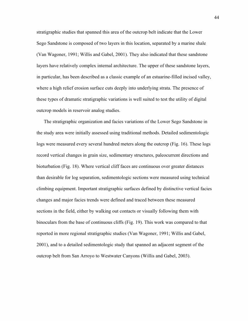
44

stratigraphic studies that spanned this area of the outcrop belt indicate that the Lower

Sego Sandstone is composed of two layers in this location, separated by a marine shale

(Van Wagoner, 1991; Willis and Gabel, 2001). They also indicated that these sandstone

layers have relatively complex internal architecture. The upper of these sandstone layers,

in particular, has been described as a classic example of an estuarine-filled incised valley,

where a high relief erosion surface cuts deeply into underlying strata. The presence of

these types of dramatic stratigraphic variations is well suited to test the utility of digital

outcrop models in reservoir analog studies.

The stratigraphic organization and facies variations of the Lower Sego Sandstone in

the study area were initially assessed using traditional methods. Detailed sedimentologic

logs were measured every several hundred meters along the outcrop (Fig. 16). These logs

record vertical changes in grain size, sedimentary structures, paleocurrent directions and

bioturbation (Fig. 18). Where vertical cliff faces are continuous over greater distances

than desirable for log separation, sedimentologic sections were measured using technical

climbing equipment. Important stratigraphic surfaces defined by distinctive vertical facies

changes and major facies trends were defined and traced between these measured

sections in the field, either by walking out contacts or visually following them with

binoculars from the base of continuous cliffs (Fig. 19). This work was compared to that

reported in more regional stratigraphic studies (Van Wagoner, 1991; Willis and Gabel,

2001), and to a detailed sedimentologic study that spanned an adjacent segment of the

outcrop belt from San Arroyo to Westwater Canyons (Willis and Gabel, 2003).

45

Fig. 16.─Study area location. A) Sego Sandstone outcrop belt in grey. Rose diagrams summarize mean paleocurrents within bedsets (modified from Willis and Gabel 2003). B) Shaded relief map of study area. Limits of the study area (large box), of the 3D outcrop model (smaller box), limits of the ~ 6.8-km wide valley fill (marked by X and Y), and the 12 sedimentological logs are shown. Exposures within San Arroyo Canyon (west side), and along the main Book Cliffs outcrop belt (east side) were used to construct outcrop models.

46

Fig. 17.─USGS topographic map of the study area. Sego Sandstone outcrops mapped and digitally

modeled shown by color codes and surveyed points in magenta. Distances between exposures in San Arroyo Canyon and those in the main Book Cliffs are between 0.7-1.7 km.

47

Fig. 18.─Sedimentological logs, datumed on the middle Lower Sego Shale, show lithology, relative amount of bioturbation and paleocurrent in their measured position (see locations in Fig. 3 and key to symbols in Fig. 19).

48

Fig. 19.─Bedding diagram constructed by tracing of surfaces and facies variations in the field between sedimentological logs. Southeast portion of bedding diagram after Willis and Gabel (2001).

49

A collection of survey base stations were placed every few hundred meters along the

axis of San Arroyo Canyon and along a road on top of the Castlegate Sandstone that

follows the margin of Grand Valley. Additional surveyed base stations were placed

within two side canyons that extended farther from the Castlegate capping road into the

Book Cliffs. One hundred and one stereographic photograph sets of the east and west

walls of San Arroyo Canyon, of exposures along the main Book Cliffs trend, and of cliffs

within smaller side canyons were collected using a Nikon D100 digital camera and a 50

mm lens. Individual sets span between 50 and 200 meters of the outcrop, with a few

exceptions that span as much as 500 meters. These photos were taken with adequate

resolution to reveal details of bedding and facies within the exposed cliff faces.

Stereographic photograph set configurations followed methods previously described in

the digital outcrop modeling workflow (Fig. 4): 1) Each set contains at least two

photographs taken from different locations; 2) Photographs were taken as normal as

possible to the outcrop face, 3) Camera lens axial vectors of these photographs vary by a

low angle (5-10˚) and converge to similar point on the outcrop, 4) the coverage of

adjacent sets overlap by at least 20 %. The configuration of some sets for

photogrammetry is better than others, reflecting lessons learned that improved methods

during the course of this study.

At least one photograph from each set was printed and taken to the field. Distinctive

small features that can be easily recognized on each set of overlapping photographs were

marked and their location determined using the reflectorless total station set up on the

nearest surveyed base station. In a few locations, where outcrops were farther from the

road, control points were surveyed from longer distances to a pole mounted reflector that

50

was carried to the appropriate location on the outcrop. For these instances it was found

that the person carrying the reflector was in a better position to mark control point

locations on the photographs than was the total station operator.

Each set of control point locations (i.e., associated with each of the 101 stereographic

photograph sets) were transformed individually into Erdas processing coordinates (as

described previously). Each set of stereographic photographs and associated transformed

control point coordinates were loaded into Leica Geosystems Suite™ and control point

locations were marked with this software on each photograph in the set. Preliminary

photogrammetric triangulations to determine camera position for each photograph used

Jacobsen’s Simple Model with robust blunder checking, because this method gave the

lowest overall RMSE of the available methods. Auto tie points were then generated, and,

if necessary, edited. In general the final model processing did not include blunder

checking, because this tended to hinder the model from converging on an iterative

solution. Although final triangulations using Jacobsen’s simple model tended to report

lower overall RMSE values than those that used Bauer’s modeling method, in some cases

the resulting digital elevation model fit less well with their neighbors in the compiled

digital outcrop model. This problem was fixed by using unmodified optical triangulation

or Bauer’s modeling method before recreation of digital elevation models and the

orthorectified photographs.

The 101 digital elevation models produced from stereographic photograph sets were

saved and transformed back into the coordinates of the field survey. Orthorectified

photographs based on each stereographic photograph set were generated. These

Orthorectified photographs were mosaiced in Erdas’ mosaic images application. The

51

corner point coordinates of each orthorectified photomosaic were saved and transformed

into coordinates of the field survey. All this data were loaded into Gocad™ for final

compilation and editing as described above in “Digital outcrop models for geologic

mapping”. Once the digital outcrop models were compiled within Gocad™ , stratigraphic

horizons were defined using 3D polygonal curves to demonstrate the usefulness of this

model for geologic mapping (Fig. 10). Three erosion surfaces (one at the base of each

sandstone layer within the Lower Sego Sandstone, and one within the upper of these two

sandstone layers), and two abrupt fining surfaces (defining the top of each of the

sandstone layers) were mapped. Isopach maps recording the stratigraphic distance from

two of these erosion surfaces to one of the abrupt fining surfaces were constructed to

demonstrate the capabilities of Gocad™ to extend surfaces mapped along outcrops into

three dimensions.

Depositional Interpretations of the Lower Sego Sandstone

The digital outcrop model produced from exposures in the area of San Arroyo

Canyon provides an unprecedented view of the stratigraphy and facies variations within

one area of the Lower Sego Sandstone. While it is beyond the scope of this project to

describe and interpret the sedimentology of these deposits in detail, general

interpretations of observed facies trends are presented below within the context of the

regional sequence stratigraphic framework developed by Willis and Gabel (2001, 2003).

General stratigraphic variations along this segment of the Book Cliffs outcrop belt are

shown in a bedding diagram constructed from the correlated logs measured along the

cliffs bordering Grand Valley (Fig. 18). Details of facies variations in different locations

along this cross section are shown in the sedimentogical logs used to construct this cross

52

section (Fig. 18). An annotated video showing a “flight” along different outcrops within

the study area shows the bedding architecture in more detail (Appendix 2).

Dark shales in the center of the Buck Tongue of the Mancos Shales record maximum

transgression of the underlying Blackhawk-Castlegate clastic wedge. Willis and Gabel

(2001, 2003) interpreted the upper Buck Tongue and Lower Sego Sandstone to record a

period of falling stage shoreline regression. Deposits of the upper Buck Tongue gradually

coarsen upward; initial shales pass upward into a mix of thoroughly marine bioturbated

clayey siltstones, and then into decimeters-thick interbeds of bioturbated clayey-

siltstones and relatively unbioturbated very-fine-grained, hummocky cross-stratified

sandstones. Ichnofossils include Planolites, Thalassinoides, Asterosoma and

Paleophycos. The upper 20 meters of this succession contains meters-thick upward-

coarsening bedsets capped by thicker beds of hummocky cross stratified sandstone. Some

of these bedsets gradually thin along depositional strike when traced for tens of

kilometers, and locally they are eroded by channel-form bodies of tidal sandstone (Willis

and Gabel, 2001). These very broadly lobate bedsets are interpreted to be distal marine

extensions of shoreline depositional lobes that were locally eroded by tidal currents.

Although the boundary between the Buck Tongue and the Lower Sego Sandstone is

formally defined lithostratigraphically as where the deposits gradually become more than

50% sandstone, in practice the base of the Lower Sego is commonly defined in local

areas at the first erosionally-based, fine- to medium-grained, tide-influenced sandstone.

Although it has been shown that such “first” erosion surfaces occur at slightly different

stratigraphic horizons along the Sego Sandstone outcrop belt, this criterion provides a

useful definition of the base of the Sego in this local study area. The first tidal erosion

53

surface is continuous across this area and displays significant erosional relief, cutting up

to 8 meters into the underlying broadly-horizontal beds of hummocky cross stratified

sandstone. Above this erosion surface is the 30 m thick interval of the Lower Sego

Sandstone (dominated by fine- to medium-grained sandstone), which ends abruptly at the

base of the nearly 10 meter thick, regionally-continuous, marine-shale-dominated interval

of the overlying Anchor Mine Tongue. The digital outcrop model presented here was

constructed to examine the internal architecture of this Lower Sego Sandstone.

The lower Sego Sandstone can be divided into two sandstone-dominated layers

separated, in most locations, by a decimeters-thick, marine-bioturbated shale (referred to

here as the middle Lower Sego shale). Both sandy layers have erosional bases.

Interpretations of the erosion surfaces at the base of these sandy layers is controversial;

Van Wagoner (1991) interpret them to be “sequence boundaries” that define the base of

fluvial incised valleys, whereas Willis and Gabel (2001) suggest that they formed by tidal

erosion in front of prograding deltaic shorelines. The later interpretation is adapted here

(they are labeled “regressive surfaces of erosion” 1 and 2 on Fig. 18, respectively).

Abrupt fining of deposits at the top of each of these sandstone-dominated layers are

interpreted by both Van Wagoner (1991) and Willis and Gabel (2001) to record

transgression (these surface, across which deposits abruptly fine, are labeled “Flooding

Surfaces” 1 and 2 on Fig. 18, respectively). The remainder of this discussion focuses on

bedding architecture and facies variations within these two sandy layers, from a

regressive surfaceof erosion to a flooding surface.

The first sandstone layer is mostly very-fine to fine grained. An isopach of this layer,

determined by mapping the basal regressive and top flooding surface on the digital

54

outcrop model, shows 6 meters of relief (Fig. 19). Although much of this relief reflects a

thinning of the deposits to the west, there are also distinct northwest-southeast trending

thicks related to local basal scours. In some locations this sandstone layer coarsens

upward, and in others it fines upward. Deposits comprise a number of meters-thick

bedsets with sheet-like or channel-form geometry. Sheet-like bedsets tend to: 1) coarsen

upward slightly as depositional beds thicken and contain fewer shale drapes, or 2) they

are extensively bioturbated by Ophiomorpha or, less commonly, Thalassinoides,

Paleophycos and Planolites.

The less bioturbated examples display abundant evidence of reversing tidal currents,

including sigmoidal dune-scale cross strata with reactivation surfaces, reversing-current

ripple scale cross lamination, and a profusion of thin mud drapes. In general more

completely bioturbated bedsets tend to be thinner, and it is common for bedsets that are

less bioturbated lower down to become more bioturbated at their top.

In a few locations channel-form bedsets cut from within this sandstone layer into the

underlying basal regressive surface, and this defines the NW-SE elongate isopach tends

(Fig. 20). These basal channel-form bedsets tend to be sandy, and contain dune-scale bi-

directional cross stratification. Most channel-form bedsets cut downward from the top of

this sandy layer (Figs. 14, 15 and 20). Those cut from the top of the sandy layer are

typically only a few hundred meters long and can fine upward and laterally from sandier

into more heterolithic beds. Many contain a set of inclined, decimeter-thick beds dipping

away from one margin, and more horizontal, channel-filling beds adjacent to an opposite

steeper cut-bank margin. The ratio of laterally-accreted (inclined) beds to channel filling

beds (on the order of 1) indicates low sinuosity channels.

55

Fig. 20.─Isopach map of lower sandstone layer. A) Thickness between the first surface of regression and overlying flooding surface (see Fig. 19). Warm colors are thicker areas associated with two basal channel belts in the southern half of the 3D volume, and an isolated channel in the northern portion of the map near Hat Rock. Blue and black points are curves mapped on the 3D model that were used as constraints for surface mapping. B) Shaded relief map of the first surface of regression (10x vertical exaggeration). C) Same shaded relief map with the isopach contours displayed. D) An isopach map of first surface of regression contoured in meters.

56

This is supported by the mapping of some of these channel bodies between adjacent sub-

parallel canyon exposures in the digital outcrop model. Internal facies locally indicate a

tidal influence. Pronounced cements, which follow basal erosion surfaces of bedsets, and

are particularly pronounced within channel filling deposits, probably reflect locations that

had thick shell lag accumulations (Fig. 20). In a few locations oyster shell casts are

observed within these cements. The top contact of this sandy layer is abrupt and

extensively bioturbated. It is interpreted to have formed during transgressive ravinement,

making it hard to infer the depositional setting of the of the underlying channel deposits.

They may be tidally-influenced fluvial or delta top tidal channels, which remained

after transgessive ravinement stripped off adjacent floodplain or tidal flat deposits.

Alternatively these deposits may record tidal channels and bars formed in subtidal area of

the shoreline.

The architecture of the second sandy layer in the Lower Sego Sandstone is more

complicated than the first. It starts at an erosional contract above the decimeters-thick

middle Lower Sego shale (i.e. the second regression surface of erosion in Fig. 18, and

Fig. 21). In many places the basal deposits of this layer are very heteroliothic and

extensively marine bioturbated (Ophiomorpha, Thalassinoides, Asterosoma Paleophycos

and Planolites). Decimeter-thick sandstones interbedded with mudstones contain

reversing dune and ripple-scale cross stratification. Just to the west of this study area

Willis and Gabel (2001) report that this layer is composed of a stack of meters-thick,

upward-coarsening tidal bar deposits, in which successive bars generally become thicker,

and sandier upsection (Fig. 19).

Within this study area the upward-coarsening succession they describe is variably

57

truncated by a high relief erosion surface that locally cuts entirely through this sandy

layer, through the middle Lower Sego Shale below, and then into the upper part of the

basal layer of the Lower Sego Sandstone (Fig. 22). This high relief erosion surface is

interpreted to be the base of a valley, incised by fluvial channels during a sea level

lowstand (an Exxon “sequence boundary”).

An isopach of the thickness between the valley floor and the underlying flooding

surface shows three NW-SE elongate areas of deeper erosion into the middle Lower Sego

shale (Fig. 23). The underlying flooding surface was used as a datum for this isopach

map instead of the overlying flooding surface because it contained less topographic relief.

Along each of these more deeply eroded trends, some recognized in the digital outcrop

models in more than one of the sub-parallel cliff exposures, are sandy channel-form

deposits dominated by ebb-oriented dune-scale cross stratification. These are interpreted

to be lowstand fluvial bypass channel deposits (Fig 22C and D).

58

Fig. 21.─Channel erosion of the middle Lower Sego Shale observed along the middle of the Northern Side Canyon (see Fig. 4). There the middle Lower Sego Shale has been eroded by tidal scour during initial sea-level fall. Overlying heterolithic tidal deposits are seen as low angle, decimeter-scale accretionary bedsets dipping to the left (Southwest). These deposits are incised by the valley.

59

Fig. 22.─Lower Sego channels observed in West Wall. A) Channel incised down from the first flooding surface cuts into underlying channel deposits along this horizon (to the right). B) Oblique view of the Northern West Wall digital outcrop model showing deepest Lower Sego channel, which completely cuts out the underlying heterolithic tidal deposits and partially erodes a hummocky sandstone deposit (see also Fig. 19, Log 6). C) Close-up view of a hummocky sandstone bed cut out by the deepest Lower Sego channel. D) Cement nodules along lateral accretion surfaces within Lower Sego channel bedsets.

60

Fig. 23.─Interpretational lines. A) Hat Rock digital outcrop model. B) Hat Rock digital outcrop model interpretation lines showing low angle tidal clinoform deposits dipping in a landward direction (see also Fig. 18, Logs 7-11).

61

Fig. 24.─Channel surface erosion into the middle Lower Sego Shale. A) Mapped surfaces of the valley floor sequence boundary (red), and base of the middle Lower Sego Shale horizon (green). Where the valley floor horizon has dropped below the base of the middle Lower Sego Shale horizon are areas where the shale is completely eroded. Note the low sinuosity channel form. B) Shaded relief map of the valley floor sequence boundary (red), and the top of the middle Lower Sego Shale (light green). Regions where the middle Lower Sego Shale is partially eroded along the sequence boundary are seen as light green (where the interpreted sequence boundary horizon drops below the top of the middle Lower Sego Shale horizon). Two minor channels flank the major channel in the middle of this diagram. C) Channel-form bedset in the West Wall outcrop. The interpretation valley floor (red) is nearly normal to this photograph (see also Fig. 23A at point X). D) Classic location in North San Arroyo Canyon where the valley’s central channel cuts through the lower Middle Sego Shale and into the underlying Lower Sego Sands (see location marked by Z in Fig. 3B).

62

Fig. 25.─Isopach maps of sequence boundary. A) Thickness between valley floor sequence boundary and the underlying flooding surface (see also Fig. 19). Warmer colors are thinner areas associated with channel erosion along the valley axis. Cooler colors are thicker areas where the base of the valley floor rises toward valley margins. Interpretation curves are seen in black. B) Shaded relief map of sequence boundary (7x vertical exaggeration). C) Shaded relief map with the isopach contours. D) Isopach map of the sequence boundary with meter contours.

63

Above the basal fluvial channel deposits the facies become more heterolithic and

evidence for tidal influence on deposition is abundant. These deposits are interpreted to

have formed in the late lowstand estuaries of the flooded river valley. There is a

pronounced cemented horizon within these heterolithic deposits that locally contains

preserved oyster shells, which could define a tidal ravinement surface formed where tides

accelerated into the mouth of the estuary.

This cemented layer becomes particularly thick where it passes over a lowstand

channel deposit, which may indicate either that these deposits remained highs during

transgression that nucleated oyster shoals, or that they allowed greater movement of

diagenetic fluids after burial. The layer is capped by a sandier bedset that is 6 m thick

near the axis of the valley fill and thins toward the valley fill margins. Inclined beds dip

northwest at a low angle from the top to base of these sets over several hundred meters (a

direction inferred to generally be landward, Fig. 24). This sandier bedset is interpreted to

record deposition of an estuary mouth shoal formed as open marine currents moved sands

along shore into the estuary mouth. The top of this bedset is heavily bioturbated by

Ophiomorpha and occasionally displays channel form geometries (Fig 25.). Like the

basal sandy interval of the lower Sego Sandstone, this one ends abruptly at a thin

erosional oyster shell lag directly overlain by marine shale. This shell lag is interpreted to

record transgressive ravinement.

64

CONCLUSIONS

Photogrammetry provides a flexible and relatively inexpensive method to construct

3D Digital Outcrop Models. Photographic sets for photogrammetric processing should: 1)

have camera lens axial vectors that vary by a low angle (5-10˚), 2) converge to a similar

point on the outcrop, 3) be nearly normal to the outcrop face, 4) adjacent photograph sets

should overlap by about 20 %. Surveyed control points should be spaced such that they

record a wide distribution of coordinate positions on photographs. Surveyed coordinates

must be rotated and transformed before photogrammetry triangulation models and

automatic tie points are generated in Erdas Photogrammetry Suite™. Digital elevation

models generated using photogrammetry can be used to orthorectify and mosaic

photograph sets within specified projection planes. Digital elevation models and

orthorectified photomossacs and be exported for use in visualization and geologic

modeling software. Gocad’s Earth Modeling software allows the coupling of digital

elevation models surfaces with orthorectified photomosaics to produce digital outcrop

models.

A field test of photogrammetry-based outcrop modeling methods was completed for

kilometers-long, sub-parallel outcrops of the Sego Sandstone in the San Arroyo Canyon

area of central Utah. Overall accuracy of digital outcrop models is 0.104m in X, 0.103m

in Y, 0.05m in Z at 90% confidence. Greatest inaccuracies within the test model were

generally associated with areas where the configuration of photographic sets relative of

the outcrop was not ideal for photogrammetry triangulation; were the focal axis and the

65

outcrop face where not normal, or where the convergence of photographs within a set

was at high angles. Geologic mapping in three dimensions using digital outcrop models

compiled in Gocad™ allows rapid surveys of stratal geometries and facies observations.

Three dimensional curves mapped on outcrop models can be interpolated between

exposures to define continuous horizons. This type of geologic mapping within a

structured, 3D coordinate system will allow the construction of outcrop analogs models

in the 3D gridded data formats required by dynamic reservoir simulators that predict

reservoir behavior.

Visualizations and surface mapping completed during the testing of photogrammetry-

based outcrop modeling methods provided insights into depositional processes within a

19 km2 area of the Lower Sego Sandstone. The model documents two progradational

sandy layers separated by a shale bed. Each layer is based by an erosion surface

(interrupted to have formed by tidal current erosion of the sea floor during falling-stage

regression), and is capped by a surface of abrupt fining to marine shale (interpreted to

record ravinement and transgression).

Complex lateral and vertical facies patterns within the first sandy layer reflect

variations across channel bodies cut into highly marine bioturbated sandstones. Local

channel bodies along the base of the layer may record subtidal erosion, whereas those

that cut downward from the top of the layer are probably distributary channels. The

proportion of inclined lateral accretion to channel filling beds within channel bodies

(about 1/1) and the mapping of individual bodies across multiple exposures documented

by the outcrop model suggest deposition in low sinuosity channels. The lateral extent of

individual inclined beds suggests channel widths less than 100 meters. Thick carbonate

66

cement nodules along bases of channel bodies and, particularly, within finer grained

channel fills are interpreted to reflect locations where shelly material was concentrated

during deposition. The lack of delta top paralic facies may indicate shoreline ravinement

during transgression.

Facies trends within the second layer are segregated by a high-relief erosion surface

that extends across the mapped area from nearly the top of this layer down through its

base. Facies below this erosion surface are initially heterolithic upward-coarsening-

bedsets that have previously been interpreted to be deposits of subtidal bars. Three areas

of deepest incision along this erosion surface are overlain by relatively sandy channel

bodies, interpreted to be the deposits of an incised lowstand fluvial system that have

subsequently been reworked by tidal processes. More heterolithic deposits higher within

the layer are interpreted to be deposits of a valley filling estuary. A capping sandstone

bedset with internal landward-dipping inclined beds is interpreted to be deposits of an

estuary mouth sand shoal. A discontinuous oyster shell lag at the top of this layer records

transgressive ravinement before deposition of marine shales of the overlying Anchor

Mine Tounge.

67

APPENDIX 1

This appendix is an instructional video of how to create a digital outcrop model.

Each chapter of the video represents a major step in the overall workflow. The techniques

used to create the faults and surfaces have not been shown.

68

APPENDIX 2

This video is a fly-by of the digital outcrop models as seen in Gocad™. Each chapter

in this video represents a single continuous digital outcrop model. This video was

constructed to provide a virtual field-trip through the study area.

69

REFERENCES

Dueholm, K.S., & Olsen, T., 1993, Reservoir analog studies using multimodel

photogrammetry: a new tool for the petroleum industry: American Association of

Petroleum Geologists Bulletin, v. 77, p. 2023–2031.

Erdman, C.E., 1934, The Book Cliffs coal field in Garfield and Mesa Counties, Colorado:

US Geol. Surv. Bull., v. 851, p. 150.

Fisher, D.J., 1936, The Book Cliffs coal field in Emert and Grand Counties, Utah: US

Geol. Surv. Bull., v. 852, p. 104

Leica, 2003, Photogrammetry Suite OrthoBASE & OrthoBASE Pro User’s Guide,

Bethesda, Maryland, American Society for Photogrammetry & Remote Sensing,.

Mc Laurin, B.T., and Steel, R.J., 2000, Fourth-order nonmarine to marine sequences,

middle Castlegate Formation, Book Cliffs, Utah: Geology, v. 28, p. 359–362.

Pringle, J., Gardiner, A. and Westerman, R., 2004a, Virtual geologic outcrops –

fieldwork and analysis made less exhaustive?: Geology Today, v. 20, p. 67-72.

Pringle, J., Westerman, A.R., Clark, J.D., Drinkwater, N.J., and Gardiner, A.R., 2004b,

3D high-resolution digital models of outcrop analogue study sites to constrain

reservoir model uncertainty: an example from Alport Castles, Derbyshire, UK:

Petroleum Geoscience, v. 10, p. 343-352.

Pringle, J.K., Clark, J.D., Westerman, A.R., Stanbrook, D.A., Gardiner, A.R., & Morgan,

B.E.F., 2001. Virtual outcrops: 3-D reservoir analogues. in: Ailleres, L. & Rawling,

T. (eds) Animations in Geology. Journal of the Virtual Explorer, v. 3. p. 2.

70

Willis, A., 2000, Tectonic control of nested sequence architecture in the Sego Sandstone,

Neslen Formation and Upper Castlegate Sandstone (Upper Cretaceous), Sevier

Foreland Basin, Utah, U.S.A.: Sedimentary Geology, v. 136, p. 277–317.

Willis, B.J., and Gabel, S.L., 2001, Sharp-based, tide-dominated deltas of the Sego

Sandstone, Book Cliffs, Utah, U.S.A.: Sedimentology, v. 48, p. 479–506.

Willis, B.J., and Gabel, S.L., 2003, Formation of deep incisions into tide dominated river

deltas: implications for the stratigraphy of the Sego Sandstone, Book Cliffs, Utah,

U.S.A.: Journal of Sedimentary Research, v. 73, p. 246-263.

Van Wagoner, J.C., 1991, High-frequency sequence stratigraphy and facies architecture

of the Sego Sandstone in the Book Cliffs of western Colorado and eastern Utah. in:

Van Wagoner, J.C., et al. (Eds.), Sequence Stratigraphy- Applications to Shelf

Sandstone Reservoirs. Tulsa, OK: American Association of Petroleum Geologists

Field Conference Guidebook, unpaginated.

Yoshida, S., 2000, Sequence and facies architecture of the upper Blackhawk Formation

and the lower Castlegate Sandstone (Upper Cretaceous), Book Cliffs, Utah, U.S.A.:

Sedimentary Geology, v. 136, p. 239–276.

Young, R.G., 1955, Sedimentary facies and intertonguing in the Upper Cretaceous of the

Book Cliffs, Utah–Colorado: Geol. Soc. Am. Bull. v. 66, p. 177–202.

71

VITA

Name: Matthew F. Fey

Address: 3410 Cartagena Dr. Corpus Christi, TX 78418

Email Address: mfey@geo.tamu.edu

Education: B.S., Geology, The State University of New York at New Paltz, 2003

M.S. Geology, Texas A&M University, 2006