FET SMALL-SIGNAL MODELLING BASED ON THE DST AND MEL ...

Progress In Electromagnetics Research B, Vol. 18, 185–204, 2009

FET SMALL-SIGNAL MODELLING BASED ON THE DSTAND MEL FREQUENCY CEPSTRAL COEFFICIENTS

R. R. Elsharkawy

Microstrip Department, Electronics Research InstituteDokki, Cairo 12622, Egypt

S. El-Rabaie

Faculty of Electronic EngineeringMenouf 32952, Egypt

M. Hindy and R. S. Ghoname

Microstrip Department, Electronics Research InstituteDokki, Cairo 12622, Egypt

M. I. Dessouky

Faculty of Electronic EngineeringMenouf 32952, Egypt

Abstract—In this paper, a new technique is proposed for field effecttransistor (FET) small-signal modeling using neural networks. Thistechnique is based on the combination of the Mel frequency cepstralcoefficients (MFCCs) and discrete sine transform (DST) of the inputsto the neural networks. The input data sets to traditional neuralsystems for FET small-signal modeling are the scattering parametersand corresponding frequencies in a certain band, and the outputs arethe circuit elements. In the proposed approach, these data sets areconsidered as forming random signals. The MFCCs of the randomsignals are used to generate a small number of features characterizingthe signals. In addition, other MFCCs vectors are calculated fromthe DST of the random signals and appended to the MFCCs vectorscalculated from the signals. The new feature vectors are used to trainthe neural networks. The objective of using these new vectors is tocharacterize the random input sequences with much more featuresto be robust against measurement errors. There are two benefits

Corresponding author: R. R. Elsharkawy ([email protected]).

186 Elsharkawy et al.

for this approach: a reduction in the number of neural networksinputs and hence a faster convergence of the neural training algorithmand robustness against measurement errors in the testing phase.Experimental results show that the proposed technique is less sensitiveto measurement errors than using the actual measured scatteringparameters.

1. INTRODUCTION

Knowledge of the equivalent circuit of an FET is very useful for thedevice performance analysis. Therefore, it is very important to useefficient tools to predict the small-signal circuit elements. Two majorsolution categories have been proposed by researchers to solve thesmall-signal modeling problem of transistors. The first trend is basedon the direct extraction of the small-signal circuit elements throughanalytic solutions [1–4]. This trend is very complicated because itdepends on finding closed form expressions to relate the scatteringparameters of the FET to the small-signal circuit elements.

The second trend is directed towards optimizing the componentvalues to closely fit the small-signal microwave scattering parametersmeasured or published for the device [5–8]. However, theequivalent circuit determination needs accurate broad-band S-parameters measurements. In fact, there are inherent errors invector network analyzer measurements, which cannot be avoided easily.Therefore, there is a need of a new approach which is more robust toerrors in the scattering parameters measurements.

Several modeling approaches based on artificial neural networksand belonging to the second category of solutions have been presentedin the literature [9–11]. Neural networks have the ability to simulatenonlinear relations with high accuracy. They can achieve a trade-off between efficiency and accuracy. Based on these advantagesof neural networks, they found a great popularity in modeling thenonlinear relations between the measured or published FET scatteringparameters and the values of the small-signal circuit elements. Thetraditional approach for this purpose is to build a single neural networkto relate all the measured scattering parameters to the small-signalcircuit elements, but this approach is time consuming and does notguarantee convergence in the training phase of the neural network.

In this paper, the MFCCs of the neural inputs in the traditionalmethod and the MFCCs of their DSTs are extracted and concatenatedto form feature vectors to be used as the new neural input vectors. Thepaper presents a study of the sensitivity of the traditional and proposed

Progress In Electromagnetics Research B, Vol. 18, 2009 187

neural models to measurement errors in the testing phase. The paperis organized as follows. Section 2 gives the basics of neural small-signal modeling. Section 3 gives the small-signal models for two metalsemiconductor field effect transistors (MESFETs), which will be usedthroughout the paper. Section 4 presents the proposed technique forFET small-signal modeling. Section 5 gives the experimental results.Finally, Section 6 gives the concluding remarks.

2. NEURAL SMALL-SIGNAL MODELLING

Artificial Neural Networks are programming paradigms that seekto emulate the microstructure of the brain, and they are usedextensively in artificial intelligence problems from simple pattern-recognition tasks to advanced symbolic manipulation. Generally,artificial neural networks are basic input and output devices, with theneurons organised in layers. They have the ability to model nonlinearrelations such as the relations between the scattering parameters andsmall-signal circuit elements in FETs. Several neural structures canbe implemented for this purpose. The multilayer perceptron (MLP)Network is one of such configurations [12, 13]. It is a feed-forwardartificial neural network that maps sets of input data onto a set ofappropriate outputs. A standard MLP neural network is shown inFig. 1. It consists of an input and an output layer with one or morehidden layers of nonlinearly-activated nodes. Each node in a layerconnects with a certain weight wij to every other node in the followinglayer, but there are no connections between the same layer neurons.

An MLP with one or more hidden layers can be used for FETsmall-signal modeling. The sigmoid function F (u) = 1/(1 + e−u) can

Layer 0

Outputs

Inputs

Layer 1

Layer L

Layer N L

. . .

. . .

. . .

. . .

Figure 1. Standard MLP neural network.


be used as an activation function for the hidden layers, and the neuronsfrom the input and output layers can have linear activation functions.Let X be the input vector to a single hidden layer neural network, theoutput vector Y can be obtained according to the following matrixequation [12, 13]:

Y = W2 ∗ F (W1∗X + B1) + B2 (1)

where W1 and W2 are weight matrices between the input and hiddenlayers and between the hidden and output layers, respectively. B1 andB2 are bias matrices for the hidden and output layers, respectively. Theneural network learns the relationship among sets of input/output data(training sets) that represents the characteristics of the componentunder consideration. First, input vectors are presented to the inputneurons and output vectors are computed. These output vectors arethen compared with desired values, and errors are computed. Errorderivatives are then calculated and summed up for each weight andbias until the whole training set has been presented to the network.These error derivatives are then used to update the weights and biasesfor neurons in the model. The training process proceeds until errorsbecome lower than the prescribed values or until the maximum numberof epochs is reached. Once a neural network is trained, its structureremains unchanged, and it will be capable of predicting outputs for allinputs whether they have been used for the training or not.

3. FET SMALL-SIGNAL MODELS

Many researchers are interested in FET small-signal modeling. Theyintroduced several models. Of such models, the model presented by

C f

CoRoR i

R f

C i

Rs

Ls

L oL i

V1

gmV1

+_

g m=gmo e-jωτ

(a) Vendelin model for a GaAs MESFET. (b) The model of the CF001-01 MESFET.

Figure 2. Two MESFET small-signal models.


Vendelin for a GaAs MESFET [14] and the model of the Mimix CF001-01 MESFET published in its datasheet in 2008. These models areillustrated in Fig. 2. The Vendelin model is valid up to 12GHz,and the model of the CF001-01 MESFET is valid up to 26 GHz.The Mimix CF001-01 MESFET is a 300µm gate in width, sub-half-micron gate in length GaAs device with Silicon Nitride passivation.The purpose of using these two models in the paper is to provethat the proposed technique for FET small-signal modeling is validfor different device types such as MESFETs and for different circuitconfigurations. Application of the proposed technique for other devicescan be performed in the future work.

4. PROPOSED NEURAL MODELLING TECHNIQUE

A direct approach to generate a neural model for a MESFET is touse the frequency values, magnitude and phase of the S-parametersas inputs to a single MLP neural network and circuit elements as theoutputs. In the proposed technique, we take the parameters of theGaAs MESFET shown in Table 1 or the CF001-01 MESFET as inputsto several neural networks and circuit elements as outputs for eachnetwork, separately. A training process can be performed with thesedata sets or other data sets.

Using all the data in any of Tables 1 or 2 as inputs for the neuralnetwork and circuit elements as outputs in a single neural structure asin the traditional method causes two problems. The first problem isthat the amount of data will be very large. The second one is that theconvergence will not be guaranteed. Thus, the proposed technique willbe used to achieve convergence and reduce the amount of input data.

Table 1. Published S-parameters for which, the Vendelin small-signalelements are given by Rf = 100Ω, Ro = 192 Ω, Cf = 0.018 pF,Ci = 0.5 pF, Co = 0.16 pF, Ri = 6.5Ω, and gm = 43 mS.

f

(GHz)S11 S21 S12 S22

Mag. Angle Mag. Angle Mag. Angle Mag. Angle2 0.96 −36 2.95 151 0.61 −15 0.021 73

4 0.89 −65.3 2.49 128 0.6 −28.56 0.036 61

6 0.83 −87.8 2.05 109.7 0.6 −40.34 0.043 55.6

8 0.78 −104.4 1.69 95 0.6 −51.18 0.047 54.8

10 0.75 −116.9 1.41 83 0.61 −61 0.049 57

12 0.73 −126 1.2 73.55 0.63 −70.13 0.052 63.4


Table 2. Published S-parameters for which, the values of the small-signal elements of the CF001-01 MESFET are given by Lg = 0.19 nH,Rg = 1 Ω, Cgs = 0.32 pF, Ri = 1.9Ω, Cgd = 0.023 pF, Gm = 66 mS,τ = 2.7 ps, Cds = 0.12 pF, Rds = 161 Ω, Rd = 1.3Ω, Ld = 0.21 nH,Rs = 1.1Ω, Ls = 0.04 nH.

f

(GHz)S11 S21 S12 S22

Mag. Angle Mag. Angle Mag. Angle Mag. Angle2 0.98 −24 4.56 156 0.02 73 0.53 −10

4 0.93 −51 4.31 136 0.04 62 0.5 −25

6 0.88 −72 3.83 118 0.05 51 0.48 −35

8 0.84 −98 3.47 100 0.06 38 0.43 −51

10 0.79 −122 2.99 82 0.06 23 0.38 −68

12 0.79 −140 2.64 67 0.07 18 0.38 −83

14 0.78 −154 2.41 55 0.07 10 0.39 −93

16 0.78 −166 2.27 44 0.07 5 0.36 −101

18 0.77 178 2.16 30 0.08 −2 0.32 −113

20 0.76 159 2.04 15 0.09 −13 0.27 −131

22 0.79 141 1.82 −2 0.09 −20 0.27 −163

24 0.78 132 1.52 −13 0.09 −21 0.3 176

26 0.81 129 1.31 −21 0.09 −19 0.39 168

The steps of the proposed technique can be summarized as follows:1. Calculate the MFCCs for the original input data considering it as

a random signal.2. Calculate the DST for the original data.3. Calculate the MFCCs for the output of step 2.4. Make a concatenation between the two vectors obtained from

steps 1 and 3 and use them as input for multiple neural networksto estimate each circuit element, separately.

5. In the training phase, use the output of step 4 with each circuitelement of the training set to train a neural network belonging tothis element.

6. In the testing phase, the measured S-parameters with measure-ment errors are used to predict the circuit elements with theirneural networks.The MFCCs technique is used to reduce the amount of input

data as all the inputs are replaced by a small number of MFCCs.


Measurement errors are similar in nature to random noise. It is knownin speaker identification, that the MFCCs can be used to characterizespeech signals in the presence of noise rather than using all the signalsamples in the identification process. The same idea is exploitedhere considering the measurement errors as noise. Extracting theMFCCs from the DST of the neural inputs can add more features tocharacterize the neural inputs in the presence of measurement errorsleading to more robust modeling.

4.1. The Discrete Sine Transform

The DST is a mathematical transform that uses sine functionsoscillating at different frequencies to transform time signals into a

Table 3. Number of epochs required in the training phase formodelling the relation between each circuit element in the Vendelinmodel and the published device parameters with the differentmodelling methods.

Method ofEstimation

R0 gm Rf Ri Ci Co CfAvg.

EpochesTraditional

Methodsingle layer

119 1668 1308 3780 333 2079 1027 1473

TraditionalMethodtwo layers

9844 959 355 154 552 2705 3434 2572

MFCCMethod

single layer138 78 1092 7 4 135 22 211

MFCCMethod

two layers2984 329 465 12 10 8 8 545

MFCC+DSTMethod

single layer5 46 478 572 140 198 155 228

MFCC+DSTMethodtwo layers

10 71 297 21 345 15 10 110


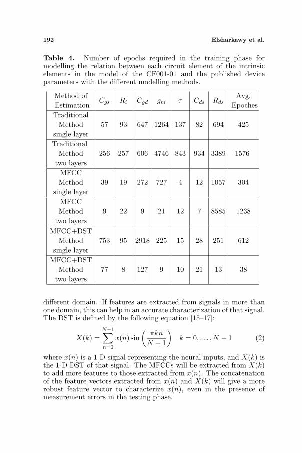
Table 4. Number of epochs required in the training phase formodelling the relation between each circuit element of the intrinsicelements in the model of the CF001-01 and the published deviceparameters with the different modelling methods.

Method ofEstimation

Cgs Ri Cgd gm τ Cds RdsAvg.

EpochesTraditional

Methodsingle layer

57 93 647 1264 137 82 694 425

TraditionalMethod

two layers256 257 606 4746 843 934 3389 1576

MFCCMethod

single layer39 19 272 727 4 12 1057 304

MFCCMethod

two layers9 22 9 21 12 7 8585 1238

MFCC+DSTMethod

single layer753 95 2918 225 15 28 251 612

MFCC+DSTMethod

two layers77 8 127 9 10 21 13 38

different domain. If features are extracted from signals in more thanone domain, this can help in an accurate characterization of that signal.The DST is defined by the following equation [15–17]:

X(k) =N−1∑

n=0

x(n) sin(

πkn

N + 1

)k = 0, . . . , N − 1 (2)

where x(n) is a 1-D signal representing the neural inputs, and X(k) isthe 1-D DST of that signal. The MFCCs will be extracted from X(k)to add more features to those extracted from x(n). The concatenationof the feature vectors extracted from x(n) and X(k) will give a morerobust feature vector to characterize x(n), even in the presence ofmeasurement errors in the testing phase.


Table 5. Number of epochs required in the training phase formodelling the relation between each circuit element of the extrinsicelements in the model of the CF001-01 and the published deviceparameters with the different modelling methods.

Method ofEstimation

Lg Rg Rd Ld Rs LsAvg.

EpochesTraditional

Methodsingle layer

64 92 6793 58 5818 1365 2365

TraditionalMethod

two layers598 8846 8325 473 10000 1756 5000

MFCCMethod

single layer6 6 6 138 13 226 66

MFCCMethod

two layers285 10 198 8 36 19 93

MFCC+DSTMethod

single layer23 511 4 36 57 1655 381

MFCC+DSTMethod

two layers243 747 11 215 22 141 230

4.2. Extraction of the MFCCs

The MFCCs of a data sequence are a representation of the short-term coefficients derived from a type of cepstral transformation of thisdata sequence. The calculation of the MFCCs is based on a linearcosine transform of a log power spectrum on a nonlinear Mel-scale offrequencies [14]. The MFCCs of a signal are commonly derived asfollows:

1. Take the Fourier transform of the signal.2. Map the powers of the spectrum obtained above onto the Mel-

scale, using triangular overlapping windows.3. Take the logs of the powers at each of the Mel-frequencies.


4. Take the DCT of the list of Mel log powers, as if they constitutea signal.

5. The MFCCs are the amplitudes of the resulting spectrum.

The Mel scale is calculated as follows:

Mel(f) = 2595 log10

(1 +

f

700

)(3)

where Mel(f) gives the Mel-scale frequency corresponding to the actualfrequency f . If the energy of the mth Mel-filter output is S(m), theMFCCs will be given as follows [2]:

cj =

√2

Nf

Nf∑

m=1

log(S(m)

)cos

(jπ

Nf(m− 0.5)

)(4)

where j = 0, 1, . . . J − 1, J is the number of MFCCs; Nf is the numberof Mel-filters; cj are the MFCCs. The number of resulting MFCCsis chosen between 12 and 20, since most of the signal information isrepresented by the first few coefficients. The 0th coefficient representsthe average log energy of the data sequence. We will choose 13coefficients in our experiments.

5. EXPERIMENTAL RESULTS

In this section, several experiments are carried out to test the proposedtechnique for FET small-signal modeling. The published S-parametersat certain frequencies for two small-signal models are used in theseexperiments. The models used are the Vendelin small-signal model ofa GaAs MESFET and the small-signal model of the Mimix CF001-01 GaAs MESFET. The published S-parameters for these models aretabulated in Tables 1 and 2.

Three methods are tested for creating neural models to estimatethe small-signal circuit elements from the published parameters. Thesemethods are the traditional neural network modeling method using allpublished data as inputs, the proposed method using the MFCCs ofthe published data, and the proposed method using a concatenationof the MFCCs obtained from the original data and MFCCs obtainedfrom the DST of this data. For all the experiments, a neural networkis created through training to relate each circuit element to the neuralinputs, whether they are the published data or features extracted fromthis data.

Two types of neural networks are considered and compared tocreate the neural models with different three methods for each circuit


element, single and two hidden layer networks. The error back-propagation algorithm is used in the network training phase for eachcase. The average numbers of epochs required in the training phasefor each neural network are tabulated in Tables 3 to 5. From thesetables, it is clear that the number of epochs required for creating the

-25 -20 -15 -10 -5 0 5 10 15 20 250

40

60

80

100

120

Max. Percentage error in measured values

Pe

rce

nta

ge

err

or

in e

stim

ate

d R

(a) (b)

0

20

40

60

80

100

120

140

160

180

200

(c) (d)

(e) (f)

o

-25 -20 -15 -10 -5 0 5 10 15 20 250

20

40

60

80

100

120


-25 -20 -15 -10 -5 0 5 10 15 20 25

0

20

40

60

80

100

120


-25 -20 -15 -10 -5 0 5 10 15 20 25

0

20

40

60

80

100

120


-25 -20 -15 -10 -5 0 5 10 15 20 250

20

40

60

80

100

120


-25 -20 -15 -10 -5 0 5 10 15 20 25


Pe

rce

nta

ge

err

or

in e

stim

ate

d g

m

Pe

rce

nta

ge

err

or

in e

stim

ate

d R

f

Pe

rce

nta

ge

err

or

in e

stim

ate

d R

i

Pe

rce

nta

ge

err

or

in e

stim

ate

d C

o

Pe

rce

nta

ge

err

or

in e

stim

ate

d C

i

20


(g)

-25 -20 -15 -10 -5 0 5 10 15 20 250

20

40

60

80

100

120


Pe

rce

nta

ge

err

or

in e

stim

ate

d C

f

Figure 3. Estimation errors for the circuit elements of Vendelin modelfor random measurement errors in the case of single hidden layer neuralnetworks.

-25 -20 -15 -10 -5 0 5 10 15 20 250

40

60

80

100

120


Pe

rce

nta

ge

err

or

in e

stim

ate

d R

(a) (b)

(c) (d)

o

-20 -15 -10 -5 0 5 10 15 20 250

20

40

60

80

100

120


-25 -20 -15 -10 -5 0 5 10 15 20 25

0

20

40

60

80

100

120


-20 -15 -10 -5 0 5 10 15 20 25

0

20

40

60

80

100

120


Pe

rce

nta

ge

err

or

in e

stim

ate

d g

m

Pe

rce

nta

ge

err

or

in e

stim

ate

d R

f

Pe

rce

nta

ge

err

or

in e

stim

ate

d R

i

-25

20


0

20

40

60

80

100

120

140

160

180

(e) (f)

-25 -20 -15 -10 -5 0 5 10 15 20 250

50

100

150

200

250


-25 -20 -15 -10 -5 0 5 10 15 20 25


Pe

rce

nta

ge

err

or

in e

stim

ate

d C

o

Pe

rce

nta

ge

err

or

in e

stim

ate

d C

i

(g)

-25 -20 -15 -10 -5 0 5 10 15 20 250

100

200

300

400

500

600


Pe

rce

nta

ge

err

or

in e

stim

ate

d C

f

700

800

Figure 4. Estimation errors for the circuit elements of Vendelin modelfor random measurement errors in the case of two hidden layers neuralnetworks.

-25 -20 -15 -10 -5 0 5 10 15 20 250

40

60

80

100

120


Pe

rce

nta

ge

err

or

in e

stim

ate

d C

(a) (b)

gs

-20 -15 -10 -5 0 5 10 15 20 250

20

40

60

80

100

120


Pe

rce

nta

ge

err

or

in e

stim

ate

d R

i

-25

20


(c) (d)

(e) (f)

-25 -20 -15 -10 -5 0 5 10 15 20 25

0

20

40

60

80

100

120


-20 -15 -10 -5 0 5 10 15 20 25

0

20

40

60

80

100

120


-25 -20 -15 -10 -5 0 5 10 15 20 250

20

40

60

80

100

120


-25 -20 -15 -10 -5 0 5 10 15 20 25


Pe

rce

nta

ge

err

or

in e

stim

ate

d C

gd

Pe

rce

nta

ge

err

or

in e

stim

ate

d g

m

Pe

rce

nta

ge

err

or

in e

stim

ate

d t

ime

de

lay

Pe

rce

nta

ge

err

or

in e

stim

ate

d C

ds

(g)

-25 -20 -15 -10 -5 0 5 10 15 20 250

20

40

60

80

100


Pe

rce

nta

ge

err

or

in e

stim

ate

d R

ds

-25

0

20

40

60

80

100

120

10

30

50

70

90

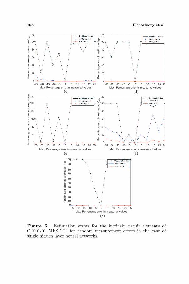
Figure 5. Estimation errors for the intrinsic circuit elements ofCF001-01 MESFET for random measurement errors in the case ofsingle hidden layer neural networks.


-25 -20 -15 -10 -5 0 5 10 15 20 250

40

60

80

100

120


Pe

rce

nta

ge

err

or

in e

stim

ate

d L

(a) (b)

(c) (d)

(e) (f)

d

-20 -15 -10 -5 0 5 10 15 20 250

20

40

60

80

100

120


-25 -20 -15 -10 -5 0 5 10 15 20 250

20

40

60

80

100

120


-20 -15 -10 -5 0 5 10 15 20 250

20

40

60

80

100

120


-25 -20 -15 -10 -5 0 5 10 15 20 250

20

40

60

80

100

120


-25 -20 -15 -10 -5 0 5 10 15 20 25


Pe

rce

nta

ge

err

or

in e

stim

ate

d R

d

Pe

rce

nta

ge

err

or

in e

stim

ate

d L

s

Pe

rce

nta

ge

err

or

in e

stim

ate

d R

s

Pe

rce

nta

ge

err

or

in e

stim

ate

d L

g

Pe

rce

nta

ge

err

or

in e

stim

ate

d R

g

-25

20

0

20

40

60

80

100

120

Figure 6. Estimation errors for the extrinsic circuit elements ofCF001-01 MESFET for random measurement errors in the case ofsingle hidden layer neural networks.


neural networks is lower for the two proposed methods than that forthe traditional method in most cases, which reveals that the proposedmethods are time saving.

In the testing phase, the neural networks are tested with inputdata subject to measurement errors. The measurement errors are

-25 -20 -15 -10 -5 0 5 10 15 2025

0

40

60

80

100

120


Pe

rce

nta

ge

err

or

in e

stim

ate

d C

(a) (b)

1000

2000

3000

4000

5000

6000

(c) (d)

(e) (f)

gs

-20 -15 -10 -5 0 5 10 15 20 250

20

40

60

80

100

120


-25 -20 -15 -10 -5 0 5 10 15 20 25

0

50

100

150

200

250

300


-20 -15 -10 -5 0 5 10 15 20 25

0

20

40

60

80

100

120


-25 -20 -15 -10 -5 0 5 10 15 20 250

50

100

150


-25 -20 -15 -10 -5 0 5 10 15 20 25


Pe

rce

nta

ge

err

or

in e

stim

ate

d R

i

Pe

rce

nta

ge

err

or

in e

stim

ate

d C

gd

Pe

rce

nta

ge

err

or

in e

stim

ate

d g

m

Pe

rce

nta

ge

err

or

in e

stim

ate

d t

ime

de

lay

Pe

rce

nta

ge

err

or

in e

stim

ate

d C

-25

20

0

-25


(g)

-25 -20 -15 -10 -5 0 5 10 15 20 250

20

40

60

80

100

120


Pe

rce

nta

ge

err

or

in e

stim

ate

d R

ds

Figure 7. Estimation errors for the intrinsic circuit elements ofCF001-01 MESFET for random measurement errors in the case of twohidden layers neural networks.

simulated as uniformly distributed random errors added to thepublished data. A comparison study is held between the sensitivityof the three methods to the measurement errors in the publishedparameters. The results of this comparison study for all elementsare given in Figs. 3 to 8. In these experiments, each circuit elementis estimated using its created neural networks for all methods witherrors having a uniform distribution added to the neural inputs. Sincethe errors in all neural inputs are not fixed, the maximum percentageerror among the neural inputs is taken as the horizontal axis, and thepercentage error in the estimated value of the circuit element is takenas the vertical axis.

Figures 3 to 8 show that the method based on the MFCCs ofthe inputs and MFCCs of DSTs of the inputs is more robust tomeasurement errors than the traditional method and in most casesbetter that using the MFCCs only based on the error pattern used.The studied cases for single and two hidden layers neural networksreveal that the use of two hidden layers does not add an advantage inthe performance of the proposed method. So, single hidden layer neuralnetworks are preferred for the task of small-signal modeling because oftheir simplicity.


-25 -20 -15 -10 -5 0 5 10 15 20 250

40

60

80

100

120


Pe

rce

nta

ge

err

or

in e

stim

ate

d L

(a) (b)

0

50

100

150

(c) (d)

(e) (f)

d

-20 -15 -10 -5 0 5 10 15 20 250

20

40

60

80

100

120


-25 -20 -15 -10 -5 0 5 10 15 20 25

050

100

150

200

250

300


-20 -15 -10 -5 0 5 10 15 20 25

0

20

40

60

80

100

120


-25 -20 -15 -10 -5 0 5 10 15 20 250

50

100

150

200

250

300


-25 -20 -15 -10 -5 0 5 10 15 20 25


Pe

rce

nta

ge

err

or

in e

stim

ate

d R

d

Pe

rce

nta

ge

err

or

in e

stim

ate

d L

s

Pe

rce

nta

ge

err

or

in e

stim

ate

d R

s

Pe

rce

nta

ge

err

or

in e

stim

ate

d L

g

Pe

rce

nta

ge

err

or

in e

stim

ate

d R

g

-25

20

180

160

140

160

140

350

400

450

500

350

Figure 8. Estimation errors for the intrinsic circuit elements ofCF001-01 MESFET for random measurement errors in the case of twohidden layers neural networks.


6. CONCLUSION

This paper has presented a new neural technique for small-signalmodeling of FET transistors. This technique is based on estimating theMFCCs of the available data sets of S-parameters and frequencies andMFCCs of DSTs of these dataset. The advantages of this techniqueare the reduction in the neural networks size and storage capacity, areduction in the training time and a large immunity to measurementerrors in the testing phase. The proposed technique has been testedon published data and succeeded to avoid the effect of measurementerrors on the estimated values of the circuit elements. Although twoMESFET models have been used for the validation of the proposedtechnique, all circuit models proposed for FETs and HEMTs can alsobe used as the method is independent on the configuration of the small-signal circuit.

ACKNOWLEDGMENT

The authors would like to acknowledge Mimix Broadband Inc. andthe Electronics group in the University of Liverpool for their supportduring the course of this research work.

REFERENCES

1. Curtice, W. R. and R. L. Camisa, “Self-consistent GaAs FETmodels for amplifier design and device diagnostics,” IEEETransactions on Microwave Theory and Techniques, Vol. 32,No. 12, December 1984.

2. Vendelin, G. D. and M. Omori, “Circuit model for the GaAsm.e.s.f.e.t. valid to 12GHz,” Electronics Letters, Vol. 11, No. 3,February 1975.

3. Berroth, M. and R. Bosch, “Broad-band determination of the FETsmall-signal equivalent circuit,” IEEE Transactions on MicrowaveTheory and Techniques, Vol. 38, No. 7, July 1990.

4. Ooi, B., Z. Zhong, and M. Leong, “Analytical extraction ofextrinsic and intrinsic FET parameters,” IEEE Transactions onMicrowave Theory and Techniques, Vol. 57, No. 2, February 2009.

5. Eskandanan, A. and S. Weinreb, “A note on experimentaldetermination of small-signal equivalent circuit of millimeter-waveFETs,” IEEE Transactions on Microwave Theory and Techniques,Vol. 41, No. 1, January 1993.


6. Ooi, B. L., M. S. Leong, and P. S. Kooi, “A novel approachfor determining the gaas MESFET small-signal equivalent-circuit elements,” IEEE Transactions on Microwave Theory andTechniques, Vol. 45, No. 12, December 1997.

7. Jarndal, A. and G. Kompa, “A new small-signal modelling ap-proach applied to GaN devices,” IEEE Transactions on MicrowaveTheory and Techniques, Vol. 53, No. 11, November 2005.

8. Shirakawa, K., H. Oikawa, T. Shimura, Y. Kawasaki, Y. Ohashi,T. Saito, and Y. Daido, “An approach to determining anequivalent circuit for HEMT’s,” IEEE Transactions on MicrowaveTheory and Techniques, Vol. 43, No. 3, March 1995.

9. Lazaro, M., I. Santamarıa, and C. Pantaleon, “Neural networksfor large- and small-signal modelling of MESFET/HEMT transis-tors,” IEEE Transactions on Instrumentation and Measurement,Vol. 50, No. 6, December 2001.

10. Devabhaktuni, V., M. Yagoub, and Q. Zhang, “A robustalgorithm for automatic development of neural-network modelsfor microwave applications,” IEEE Transactions on MicrowaveTheory and Techniques, Vol. 49, No. 12, December 2001.

11. Shirakawa, K., M. Shimiz, N. Okubo, and Y. Daido, “Alarge-signal characterization of an HEMT using a multilayeredneural network,” IEEE Transactions on Microwave Theory andTechniques, Vol. 45, No. 9, September 1997.

12. Galushkin, A. I., Neural Networks Theory, Springer-Verlag,Berlin, Heidelberg, 2007.

13. Dreyfus, G., Neural Networks Methodology and Applications,Springer-Verlag, Berlin, Heidelberg, 2005.

14. Vendelin, G. D., “Feedback effects in the GaAs MESFET model,”IEEE Transactions on Microwave Theory and Techniques,June 1976.

15. Guillemain, P. and R. K. Martinet, “Characterization of acousticsignals through continuous linear time-frequency representations,”Proceedings of the IEEE, Vol. 84, No. 4, 561–585, April 1996.

16. Prochazka, A., J. Uhlir, P. J. W. Rayner, and N. J. Kingsbury,Signal Analysis and Prediction, Birkhauser Inc., 1998.

17. Wornell, G. W., “Emerging applications of multirate signalprocessing and wavelets in digital communications,” Proceedingsof the IEEE, Vol. 84, No. 4, 586–603, April 1996.

FET SMALL-SIGNAL MODELLING BASED ON THE DST AND MEL ...

Documents

Transcript of FET SMALL-SIGNAL MODELLING BASED ON THE DST AND MEL ...