
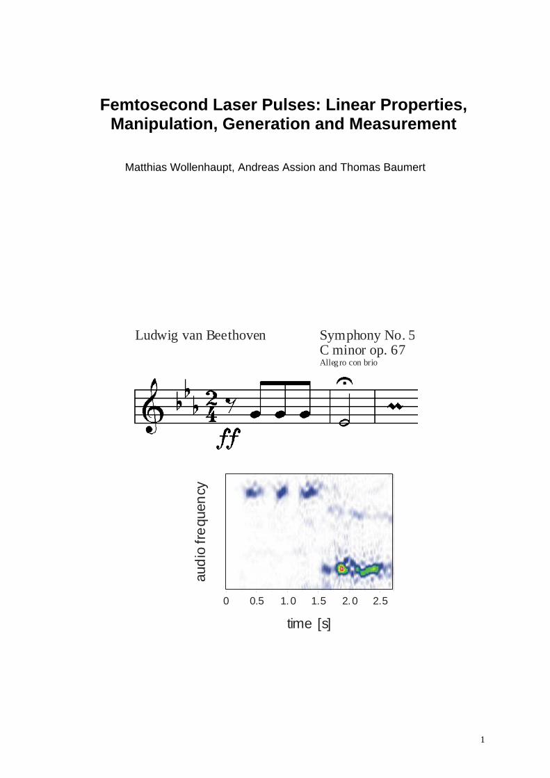
Measuring the Frequency of Light using Femtosecond Laser Pulses
1
Femtosecond Laser Pulses: Linear Properties, Manipulation, Generation and Measurement
Matthias Wollenhaupt, Andreas Assion and Thomas Baumert
time [s]
aud
io fr
equ
ency
Ludwig van Beethoven Symphony No. 5C minor op. 67Allegro con brio
0 0.5 1.0 1.5 2.0 2.5
2
Femtosecond Laser Pulses: Linear Properties, Manipulation, Generation and Measurement
Matthias Wollenhaupt, Andreas Assion and Thomas Baumert*
Universität Kassel, Fachbereich Naturwissenschaften, Institut für Physik and
Center for Interdisciplinary Nanostructure Science and Technology (CINSaT)
CONTENT
1. Introduction 2. Linear properties of ultrashort light pulses 2.1 Descriptive introduction 2.2 Mathematical description 2.3 Changing the temporal shape via the frequency domain 2.3.1 Dispersion due to transparent media 2.3.2 Angular dispersion 2.3.2.1 Prism sequences 2.3.2.2 Grating arrangements 2.3.3 Dispersion due to interference (Gires-Tournois interferometers and chirped mirrors) 2.3.4 Pulse shaping 3. Generation of femtosecond laser pulses via mode locking 4. Measurement techniques for femtosecond laser pulses 4.1 Streak camera 4.2 Intensity autocorrelation and crosscorrelation 4.3 Interferometric autocorrelations 4.4 Time frequency methods 4.4.1 Spectrogram based methods 4.4.2 Sonogram based methods 4.3 Spectral interferometry * corresponding author
3
1. Introduction A central building block for generating femtosecond light pulses are lasers. Only within two decades after the invention of the laser the duration of the shortest pulse shrunk by six orders of magnitude from the nanosecond regime to the femtosecond regime. Nowadays femtosecond pulses in the range of 10 fs and below can be generated directly from compact and reliable laser oscillators and the temporal resolution of measurements has outpaced the resolution even of modern sampling oscilloscopes by orders of magnitude. With the help of some simple comparisons the incredibly fast femtosecond time scale can be put into perspective: For example on a logarithmic time scale one minute is approximately half-way between 10 fs and the age of the universe. Taking the speed of light in vacuum into account, a 10 fs light pulse can be considered as a 3 µm thick slice of light whereas a light pulse of one second spans approximately the distance between earth and moon. It is also useful to realize that the fastest molecular vibrations in nature have an oscillation time of about 10 fs. It is the unique attributes of these light pulses that open up new frontiers both in basic research and for applications: The ultrashort pulse duration for example allows to freeze the motion of electrons and molecules by making use of so called pump probe techniques that work similar to strobe light techniques. In chemistry complex reaction dynamics have been measured directly in the time domain and this work was rewarded with the Nobel price in chemistry for A.H. Zewail in 1999. The broad spectral width can be used for example in medical diagnostics or - by taking the longitudinal frequency comb mode structure into account - for high precision optical frequency metrology. The latter is expected to outperform today’s state of the art caesium clocks and was rewarded with the 2005 Nobel price in physics for J.L. Hall and T.W. Hänsch. The extreme concentration of a modest energy content in focused femtosecond pulses delivers high peak intensities that are used for example in a reversible light matter interaction regime for the development of nonlinear microscopy techniques. The irreversible light matter regime can be for example applied to non thermal material processing leading to precise microstructures in a whole variety of solid state materials. Finally the high pulse repetition rate is exploited for example in telecommunication applications. These topics have been reviewed recently in (Keller, 2003). The biannual international conference series “Ultrafast Phenomena” and “Ultrafast Optics” including the corresponding conference proceedings cover a broad range of applications and latest developments. In this contribution some basic properties of femtosecond laser pulses are summarized. In chapter two we start with the linear properties of ultrashort light pulses. Nonlinear optical effects that would alter the frequency spectrum of an ultrashort pulse are not considered. However, due to the large bandwidth, the linear dispersion is responsible for dramatic effects. For example, a 10 fs laser pulse at a center wavelength of 800 nm propagating through 4 mm of BK7 glas will be temporally broadened to 50 fs. In order to describe and manage such dispersion effects a mathematical description of an ultrashort laser pulse is given first before we continue with methods how to change the temporal shape via the frequency domain. The chapter ends with a paragraph on the powerful technique of pulse shaping which can be used to create complex shaped ultrashort laser pulses with respect to phase, amplitude and polarization state.

4
In chapter 3 the generation of femtosecond laser pulses via mode locking is described in simple physical terms. As femtosecond laser pulses can be generated directly from a wide variety of lasers with wavelengths ranging from the ultraviolet to the infrared no attempt is made to cover the different technical approaches. In chapter 4 we deal with the measurement of ultrashort pulses. Traditionally a short event has been characterized with the aid of an even shorter event. This is not an option for ultrashort light pulses. The characterization of ultrashort pulses with respect to amplitude and phase is therefore based on optical correlation techniques that make use of the short pulse itself. Methods operating in the time-frequency domain are especially useful. Besides the specific literature given in the individual chapters some textbooks devoted to ultrafast laser pulses are recommended for a more in depth discussion of the topics presented here and beyond (see for example (Wilhelmi and Herrmann, 1987) (Akhmanov et al., 1992) (Diels and Rudolph, 1996) (Rulliere, 1998) and especially for the measurement of ultrashort pulses see (Trebino, 2000)). Finally the authors would like to acknowledge Marc Winter for help in preparing various figures.
5
2. Linear properties of ultrashort light pulses 2.1 Descriptive introduction It is quite easy to construct the electric field of a “Gedanken” optical pulse at a fixed position in space, corresponding to the physical situation of a fixed detector in space. Assuming the light field to be linearly polarized, we may write the real electric field strength E(t) as a scalar quantity whereas a harmonic wave is multiplied with a temporal amplitude or envelope function A(t) (2.1) 0 0( ) ( )cos( )E t A t tω= Φ +
with ω0 being the carrier circular (or angular) frequency. The light frequency is given
by 00 2
ωνπ
= . In the following angular frequencies and frequencies are only
distinguished from each other via their notation. For illustration we will use optical pulses centered at 800 nm corresponding to a carrier frequency of ω0 = 2.35 rad/fs (oscillation period T = 2.67 fs) with a Gaussian envelope function (the numbers refer to pulses that are generated by the widely spread femtosecond laser systems based on Titanium:Sapphire as the active medium). For simple envelope functions the pulse duration ∆t is usually defined by the FWHM (full width at half maximum) of the temporal intensity function I(t)
(2.2) 20
1( ) ( )
2=I t c n A tε
with ε0 being the vacuum permittivity, c the speed of light and n the refractive index. The factor ½ arises from averaging the oscillations. If the temporal intensity is given in W/cm2 the temporal amplitude A(t) (in V/cm for n = 1) is given by
(2.3) 0
2( ) ( ) 27.4 ( )A t I t I t
cε= =
Fig. 2.1 (a) displays E(t) for a Gaussian pulse with ∆t = 5 fs and Φ0 = 0. At t = 0 the electric field strength reaches its maximum value. This situation is called a “cosine pulse”: For Φ0 = -π/2 we get a ”sine pulse” E(t) = A(t) sin(ω0t) (see Fig 2.1 (b)) where the maxima of the carrier oscillations do not coincide with the maximum of the envelope A(t) at t = 0 and the maximum value of E(t) is therefore smaller than in a cosine pulse. In general Φ0 is termed the absolute phase or carrier-envelope phase and determines the temporal relation of the pulse envelope with respect to the underlying carrier oscillation. The absolute phase is not important if the pulse envelope A(t) does not significantly vary within one oscillation period T. The longer the temporal duration of the pulses the better this condition is met and the decomposition of the electric field into an envelope function and a harmonic oscillation with carrier frequency ω0 (see Eq. (2.1)) is meaningful. Conventional pulse characterization methods as described in chapter 4 are not able to measure the absolute value of Φ0. Furthermore the absolute phase does not remain stable in a conventional femtosecond laser system. Progress in controlling and measuring the

6
t [fs]
(b)
-10 100 5-5
t [fs]
(c)
-10 100 5-5
0
t [fs]
(a)
-10 100 5-5
0
A(t)
t [fs]
(d)
-10 100 5-5
0
E(t
)
E(t
)
E(t
)
E(t
)
0
Figure 2.1 Electric field E(t) and temporal amplitude function A(t) for a cosine pulse (a), a sine pulse (b), an up chirped pulse (c) and a down chirped pulse (d). The pulse duration in all cases is ∆t = 5 fs. For (c) and (d) the parameter a was chosen to be ± 0.15 / fs2 respectively. absolute phase has been made only recently (Jones et al., 2000;Apolonski et al., 2000;Helbing et al., 2002;Kakehata et al., 2002) and experiments depending on the absolute phase start to appear (Paulus et al., 2001) (Ye et al., 2002) (Baltuska et al., 2003). In the following we will not emphasize the role of Φ0 any more. In general we may add an additional time dependent phase function Φa(t) to the temporal phase term in Eq. (2.1) (2.4) Φ(t )= Φ0 + ω0t + Φa(t) and define the momentary or instantaneous light frequency ω(t) as
(2.5) 0
( )( )( ) ad td tt
dt dtω ω ΦΦ= = +
This additional phase function describes variations of the frequency in time denoted as chirp. In Fig. 2.1 (c) and (d) Φa(t) is set to be at2. For a = 0.15 / fs2 we see a linear increase of the frequency in time denoted as linear up chirp. For a = -0.15 / fs2 a linear down chirped pulse is obtained with a linear decrease of the frequency in time. However, a direct manipulation of the temporal phase cannot be achieved by any electronic device. Note that nonlinear optical processes like for example self phase modulation (SPM) are able to influence the temporal phase and lead to a change in the frequency spectrum of the pulse. In this contribution we will mainly focus on linear optical effects where the spectrum of the pulse is unchanged and changes in the temporal pulse shape are due to manipulations in the frequency domain (see chapter 2.3). Before we start, a more mathematical description of an ultrashort light pulse is presented.

7
2.2 Mathematical description For the mathematical description we followed the approaches of (Bradley and New, 1974;Cohen, 1995;Mandel and Wolf, 1995;Iaconis and Walmsley, 1999;Feurer et al., 2000;Bracewell, 2000), (Diels and Rudolph, 1996). In linear optics the superposition principle holds and the real-valued electric field E(t) of an ultrashort optical pulse at a fixed point in space has the Fourier decomposition into monochromatic waves
(2.6) 1
( ) ( )2
i tE t E e dωω ωπ
∞
−∞
= ∫ �
The in general complex valued spectrum ( )E ω� is obtained by the Fourier inversion theorem
(2.7) ( ) ( ) i tE E t e dtωω∞
−
−∞
= ∫�
Since E(t) is real valued ( )E ω� is hermitian, i.e. obeys the condition (2.8) * *( ) ( ) and denotes complex conjugationE Eω ω= −� � Hence knowledge of the spectrum for positive frequencies is sufficient for a full characterization of the light field and we can define the positive part of the spectrum (2.9) ( ) ( ) 0 0 0E E for and forω ω ω ω+ = ≥ <� � The negative part of the spectrum ( )E ω−� is defined as (2.10) ( ) ( ) 0 0 0E E for and forω ω ω ω− = < ≥� � Just as the replacement of real-valued sines and cosines by complex exponentials often simplifies Fourier analysis, so too does the use of complex valued functions in place of the real electric field E(t). For this purpose we separate the Fourier transform integral of E(t) into two parts. The complex valued temporal function ( )E t+ contains only the positive frequency segment of the spectrum. In communication theory and optics ( )E t+ is termed the analytic signal (its complex conjugate is
( )E t− and contains the negative frequency part). By definition ( )E t+ and ( )E ω+� as
well as ( )E t− and ( )E ω−� are Fourierpairs where only the relations for the positive frequency part are given below
(2.11) 1
( ) ( )2
i tE t E e dωω ωπ
∞+ +
−∞
= ∫ �
(2.12) ( ) ( ) i tE E t e dtωω∞
+ + −
−∞
= ∫�
These quantities relate to the real electric field
8
(2.13) { } { }( ) ( ) ( ) 2Re ( ) 2Re ( )E t E t E t E t E t+ − + −= + = =
and its complex Fourier transform (2.14) ( ) ( ) ( )E E Eω ω ω+ −= +� � �
( )E t+ is complex valued and can therefore be expressed uniquely in terms of its amplitude and phase
(2.15)
0 0
0 0
0 0
0 0
( )
( )
( )
0
( )
( ) ( )
( )
( )
2
1( )
2
( )
a
a
a
i t
i i t i t
i i t i t
i i t i t
i i tc
E t E t e
E t e e e
I te e e
cn
A t e e e
E t e e
ω
ω
ω
ω
ε
+ + Φ
Φ Φ+
Φ Φ
Φ Φ
Φ
=
=
=
=
=
where the meaning of A(t), Φ0, ω0 and Φa(t) is the same as in chapter 2.1 and Ec(t) is the complex valued envelope function without the absolute phase and without the rapidly oscillating carrier frequency phase factor, a quantity often used in ultrafast optics. The envelope function A(t) is given by
(2.16) ( ) 2 ( ) 2 ( ) 2 ( ) ( )A t E t E t E t E t+ − + −= = =
and coincides with the less general expression in Eq. (2.1). The complex positive frequency part ( )E ω+� can be analogoulsy decomposed into amplitude and phase
(2.17)
( )
( )
0
( ) ( )
( )
i
i
E E e
I ecn
φ ω
φ ω
ω ω
π ωε
+ + −
−
=
=
� �
( )E ω+� is the spectral amplitude, φ(ω) is the spectral phase and ( )I ω is the spectral
intensity – the familiar quantity measured with a spectrometer. From Eq. (2.8) the relation -φ(ω) = φ(-ω) is obtained. As will be shown in chapter 2.3 it is precisely the manipulation of this spectral phase φ(ω) in the experiment which - by virtue of the Fourier transformation Eq. (2.11) – creates changes in the real electric field strength E(t) (Eq. (2.13)) without changing ( )I ω . If the spectral intensity ( )I ω is manipulated as well, additional degrees of freedom are accessible for generating temporal pulse shapes at the expense of lower energy. Note that the distinction between positive and negative frequency parts is made for mathematical correctness. In practice only real electric fields and positive frequencies are displayed. Moreover, as usually only the shape and not the absolute magnitude of the envelope functions in addition to the phase function are the quantities of interest, all the prefactors are commonly omitted.
9
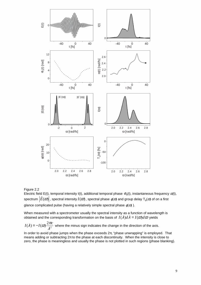
Figure 2.2 Electric field E(t), temporal intensity I(t), additional temporal phase Φa(t), instantaneous frequency ω(t),
spectrum ( )E ω� , spectral intensity ( )I ω , spectral phase φ(ω) and group delay Tg(ω) of on a first
glance complicated pulse (having a relatively simple spectral phase φ(ω) ). When measured with a spectrometer usually the spectral intensity as a function of wavelength is obtained and the corresponding transformation on the basis of ( ) ( )I d I dλ λ ω ω= yields
2
2( ) ( )
cI I
πλ ωλ
= − where the minus sign indicates the change in the direction of the axis.
In order to avoid phase jumps when the phase exceeds 2π, “phase unwrapping” is employed. That means adding or subtracting 2π to the phase at each discontinuity. When the intensity is close to zero, the phase is meaningless and usually the phase is not plotted in such regions (phase blanking).
I(t)
-40 0 40
0
E(t
)-40 0 40
0
-40 0 40
Φa(
t) [r
ad]
12
8
4
0
ω(t
) [r
ad/fs
]
-40 0 40
2.6
2.4
2.2
2.0
t [fs]
t [fs]
t [fs]
t [fs]
φω(
) [r
ad]
ω [rad/fs]2.22.0 2.4 2.6 2.8
20
10
0
T(
) [fs
]g
ω
ω [rad/fs]2.22.0 2.4 2.6 2.8
-100
-50
0
I()
ω
2.22.0 2.4 2.6 2.8
0
ω [rad/fs]
|E ( )|+ ω
ω [rad/fs]0 2-2
0
|E(
)|ω
|E ( )|- ω

10
The temporal phase Φ(t) (Eq. (2.4)) contains frequency vs. time information leading to the definition of the instantaneous frequency ω(t) (Eq. (2.5)). In a similar fashion φ(ω) contains time vs. frequency information and we can define the group delay Tg(ω) which describes the relative temporal delay of a given spectral component (see also chapter 2.3).
(2.18) ( )g
dT
d
φωω
=
All quantities discussed so far are displayed in Fig. 2.2 on behalf of an on the first glance complicated pulse. Usually the spectral amplitude is distributed around a center frequency (or carrier frequency) ω0. Therefore – for "well behaved" pulses - it is often helpful to expand the spectral phase into a Taylor series
(2.19) 0
( )( )0
0 00
2 30 0 0 0 0 0 0
( ) ( )( ) ( ) ( )
!
1 1( ) '( ) ( ) ''( ) ( ) '''( ) ( ) ...
2 6
j jj j
jj
withj ω
φ ω φ ωφ ω ω ω φ ωω
φ ω φ ω ω ω φ ω ω ω φ ω ω ω
∞
=
∂= ⋅ − =∂
= + ⋅ − + ⋅ − + ⋅ − +
∑
The spectral phase coefficient of zeroth order describes in the time domain the absolute phase (Φ0 = -φ(ω0)). The first order term leads to a temporal translation of the envelope of the laser pulse in the time domain (Fourier shift – theorem) but not to a translation of the carrier. A positive 0'( )φ ω corresponds to a shift towards later times. An experimental distinction between the temporal translation of the envelope via linear spectral phases in comparison to the temporal translation of the whole pulse is for example discussed in (Albrecht et al., 1999;Präkelt et al., 2004). The coefficients of higher order are responsible for changes in the temporal structure of the electric field. The minus sign in front of the spectral phase in Eq. (2.17) is chosen so that a positive 0''( )φ ω corresponds to a linearly up-chirped laser pulse. For illustrations see Figs. 2.2 and 2.3 (a)-(e). There is a variety of analytical pulse shapes where the above formalism can be applied to get analytical expressions in both domains. For general pulse shapes a numerical implementation is helpful. For illustrations we will focus on a Gaussian laser pulse ( )inE t+ (not normalized to pulse energy) with a corresponding spectrum
( )inE ω+� . Phase modulation in the frequency domain leads to a spectrum ( )outE ω+� with
a corresponding electric field ( )outE t+ .
(2.20)
2
20
2ln 20( )
2
ti tt
in
EE t e eω−
+ ∆=
Here ∆t denotes the FWHM of the corresponding intensity I(t). The absolute phase is set to zero, the carrier frequency is set to ω0, additional phase terms are set to zero as well. The pulse is termed an unchirped pulse in the time domain. For ( )inE ω+� we obtain the spectrum

11
(2.21) 2
2( )0 8ln 2( )2 2 ln 2
ot
in
E tE e
ω ωπω∆− −+ ∆=�
The FWHM of the temporal intensity profile I(t) and the spectral intensity profile ( )I ω are related by ∆t ∆ω = 4 ln2 where ∆ω is the FWHM of the spectral intensity profile
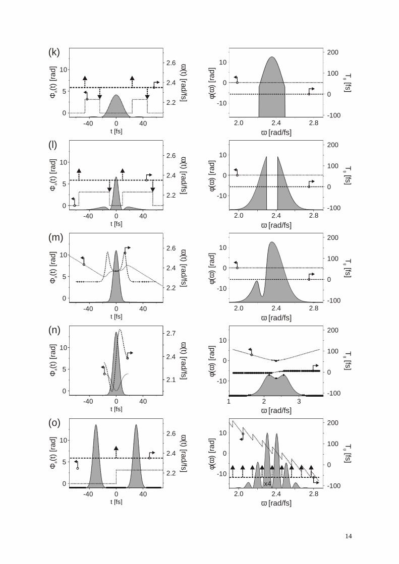
( )I ω . Figure 2.3 Examples for changing the temporal shape of a 800 nm 10 fs pulse via the frequency domain (except n). Left: Temporal intensity I(t) (shaded), additional temporal phase Φa(t) (dotted), instantaneous frequency ω(t) (dashed), Right: spectral intensity ( )I ω (shaded), spectral phase φ(ω) (dotted) and group delay Tg(ω) (dashed) for a a) bandwidth limited Gaussian laser pulse of 10 fs duration b) bandwidth limited Gaussian laser pulse of 10 fs duration shifted in time to -20 fs due to a linear phase term in the spectral domain (φ’ = -20 fs) c) symmetrical broadened Gaussian laser pulse due to φ’’ = 200 fs2 d) third order spectral phase (φ’’’ = 1000 fs3) leading to a quadratic group delay. The central frequency of the pulse arrives first, while frequencies on either side arrive later. The two corresponding slightly differences in frequencies cause beats in the temporal intensity profile. Pulses with cubic spectral phase distortion have therefore oscillations after (or before) a main pulse depending on the sign of φ’’’. The higher the side pulses, the less meaningful is a FWHM pulse duration. e) combined action of all spectral phase coefficients a)-d). Phase unwrapping and blanking is employed when appropriate f) π step at the central frequency g) π step displaced from central frequency h) sine modulation at central frequency with φ(ω) = 1 sin(20 fs (ω-ω0)) i) cosine modulation at central frequency with φ(ω) = 1 cos(20 fs (ω-ω0)) j) sine modulation at central frequency with φ(ω) = 1 sin(30 fs (ω-ω0)) Amplitude modulation: k) symmetrical clipping of spectrum l) blocking of central frequency components m) off center absorption Modulation in time domain n) self-phase modulation. Note the spectral broadening o) double pulse with pulse to pulse delay of 60 fs

12
t [fs]
Φa(
t) [r
ad] ω
(t) [rad/fs]
0
5
102.6
2.4
2.2
(d)
-40 0 40
t [fs]
Φa(
t) [r
ad] ω
(t) [rad/fs]
0
5
102.6
2.4
2.2
(c)
-40 0 40
t [fs]
Φa(
t) [r
ad] ω
(t) [rad/fs]
0
5
102.6
2.4
2.2
(e)
-40 0 40
t [fs]
Φa(
t) [r
ad]
ω(t) [rad/fs]
0
5
102.6
2.4
2.2
(b)
-40 0 40
t [fs]
Φa(t
) [r
ad] ω
(t) [rad/fs]
0
5
102.6
2.4
2.2
(a)
-40 0 40
φ()
[rad
]ω
ω [rad/fs]
10
0
-10
2.0 2.4 2.8
200
100
0
-100
T [fs]
g
φ()
[rad
]ω
ω [rad/fs]
10
0
-10
2.0 2.4 2.8
200
100
0
-100
T [fs]
g
φ()
[rad
]ω
ω [rad/fs]
10
0
-10
2.0 2.4 2.8
200
100
0
-100
T [fs]
g
φ()
[rad
]ω
ω [rad/fs]
10
0
-10
2.0 2.4 2.8
200
100
0
-100
T [fs]
g
φ()
[rad
]ω
ω [rad/fs]
10
0
-10
2.0 2.4 2.8
200
100
0
-100
T [fs]
g

13
t [fs]
Φa(
t) [r
ad] ω
(t) [rad/fs]
0
5
102.6
2.4
2.2
(f)
-40 0 40
φω(
) [r
ad]
ω [rad/fs]
10
0
-10
2.0 2.4 2.8
200
100
0
-100
T [fs]
g
t [fs]
Φa(
t) [r
ad] ω
(t) [rad/fs]
0
5
102.6
2.4
2.2
(g)
-40 0 40
φ()
[rad
]ω
ω [rad/fs]
10
0
-10
2.0 2.4 2.8
200
100
0
-100
T [fs]
g
t [fs]
Φa(t
) [r
ad] ω
(t) [rad/fs]
0
5
102.6
2.4
2.2
(h)
-40 0 40
φ()
[rad
]ω
ω [rad/fs]
10
0
-10
2.0 2.4 2.8
200
100
0
-100
T [fs]
g
t [fs]
Φa(t
) [r
ad] ω
(t) [rad/fs]
0
5
102.6
2.4
2.2
(i)
-40 0 40
φ()
[rad
]ω
ω [rad/fs]
10
0
-10
2.0 2.4 2.8
200
100
0
-100
T [fs]
g
t [fs]
Φa(
t) [r
ad] ω
(t) [rad/fs]
0
5
102.6
2.4
2.2
(j)
-40 0 40
φ()
[rad
]ω
ω [rad/fs]
10
0
-10
2.0 2.4 2.8
200
100
0
-100
T [fs]
g
14
t [fs]
Φa(
t) [r
ad] ω
(t) [rad/fs]
2.6
2.4
2.2
(k)
-40 0 40
φ()
[rad
]ω
ω [rad/fs]
10
0
-10
2.0 2.4 2.8
200
100
0
-100
T [fs]
g
t [fs]
Φa(
t) [r
ad] ω
(t) [rad/fs]
2.6
2.4
2.2
(l)
-40 0 40φ(
) [r
ad]
ω
ω [rad/fs]
10
0
-10
2.0 2.4 2.8
200
100
0
-100
T [fs]
g
t [fs]
Φa(t
) [r
ad] ω
(t) [rad/fs]
2.6
2.4
2.2
(m)
-40 0 40
φ()
[rad
]ω
ω [rad/fs]
10
0
-10
2.0 2.4 2.8
200
100
0
-100
T [fs]
g
t [fs]
Φa(
t) [r
ad] ω
(t) [rad/fs]
(n)
-40 0 40
φ()
[rad
]ω
10
0
-10
2
200
100
0
-100
T [fs]
g
t [fs]
Φa(t
) [r
ad] ω
(t) [rad/fs]
(o)
-40 0 40
0
5
10
0
5
10
0
5
10
0
5
10
0
5
10
2.7
2.4
2.1
1 3
2.6
2.4
2.2
2.0 2.4 2.8
ω [rad/fs]
φ()
[rad
]ω
ω [rad/fs]
10
0
-10
200
100
0
-100
T [fs]
g
x4

15
-40 0 40
-40 0 40
1 2 3 4
1 2 3 4
-40 0 40 1 2 3 4
1 2 3 4-40 0 40
-40 0 40
1 2 3 4
Gaussian
HyperbolicSechant
Square
Single SidedExponential
SymmetricExponential
0.441
0.315
0.886
0.110
0.142
1.414
Shape I(t) I( )ω ∆ν ∆ t ∆ ∆t / tintAC
1.543
1.000
2.000
2.421
Table 2.1 Temporal and spectral intensity profiles and time bandwidth products (∆ν ∆t ≥ K) of various pulse shapes; ∆ν and ∆t are FWHM quantities of the corresponding intensity profiles. The ratio ∆tintAC / ∆t where ∆tintAC is the FWHM of the intensity autocorrelation with respect to background (see chapter 4.2) is given in addition. In the following formulas employed in the calculations we set ω0 = 0 for simplicity.
Gaussian: ( )2
2ln 20
2
t
tEE t e
− + ∆ = , ( )2
2
0 8 2
2 2ln 2
t
lnE tE e
ωπω∆−+ ∆=�
Sech: ( ) ( )0 2ln 1 22
E tE t Sech
t+ = + ∆
( ) ( ) ( )04ln 1 2 4ln 1 2
tE E t Sech
π πω ω+ ∆ = ∆ + +
�
Rect: ( ) 0 , ,02 2 2
E t tE t t elsewhere+ ∆ ∆ = ∈ −
( ) 0
2 2
E t tE Sincω ω+ ∆ ∆ =
�
Single sided Exp: ( ) [ ]ln 2
0 2 0, , 02
t
tEE t e t elsewhere
−+ ∆= ∈ ∞ , ( ) 0
2 ln 2
E tE
i tω
ω+ ∆=
∆ +�
Symmetric Exp: ( ) ln 20
2
t
tEE t e
−+ ∆= , ( ) 02 2 2
ln 2
(ln 2)
E tE
tω
ω+ ∆=
∆ +�
16
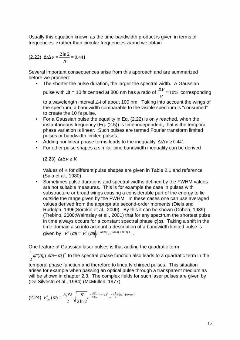
Usually this equation known as the time-bandwidth product is given in terms of frequencies ν rather than circular frequencies ω and we obtain
(2.22) 2ln 2
0.441t νπ
∆ ∆ = =
Several important consequences arise from this approach and are summarized before we proceed:
• The shorter the pulse duration, the larger the spectral width. A Gaussian
pulse with ∆t = 10 fs centred at 800 nm has a ratio of 10%ν
ν∆ ≈ corresponding
to a wavelength interval ∆λ of about 100 nm. Taking into account the wings of the spectrum, a bandwidth comparable to the visible spectrum is “consumed” to create the 10 fs pulse.
• For a Gaussian pulse the equality in Eq. (2.22) is only reached, when the instantaneous frequency (Eq. (2.5)) is time-independent, that is the temporal phase variation is linear. Such pulses are termed Fourier transform limited pulses or bandwidth limited pulses.
• Adding nonlinear phase terms leads to the inequality 0.441t ν∆ ∆ ≥ . • For other pulse shapes a similar time bandwidth inequality can be derived
(2.23) t Kν∆ ∆ ≥
Values of K for different pulse shapes are given in Table 2.1 and reference (Sala et al., 1980)
• Sometimes pulse durations and spectral widths defined by the FWHM values are not suitable measures. This is for example the case in pulses with substructure or broad wings causing a considerable part of the energy to lie outside the range given by the FWHM. In these cases one can use averaged values derived from the appropriate second-order moments (Diels and Rudolph, 1996;Sorokin et al., 2000). By this it can be shown (Cohen, 1989) (Trebino, 2000;Walmsley et al., 2001) that for any spectrum the shortest pulse in time always occurs for a constant spectral phase φ(ω). Taking a shift in the time domain also into account a description of a bandwidth limited pulse is given by 0 0 0( ) '( )( )( ) ( ) i iE E e eφ ω φ ω ω ωω ω − − −+ +=� � .
One feature of Gaussian laser pulses is that adding the quadratic term
20 0
1''( ) ( )
2φ ω ω ω⋅ − to the spectral phase function also leads to a quadratic term in the
temporal phase function and therefore to linearly chirped pulses. This situation arises for example when passing an optical pulse through a transparent medium as will be shown in chapter 2.3. The complex fields for such laser pulses are given by (De Silvestri et al., 1984) (McMullen, 1977)
(2.24) 2
2 21( ) ''( ) ( )
0 8ln 2 2( )2 2 ln 2
o o ot
i
out
E tE e e
ω ω φ ω ω ωπω∆− − − ⋅ −+ ∆=�
17
(2.25)
2
20 ( )40
1
4
2 2
02 2
( )
2
'' '' 1 ''1 arctan( )
8ln 2 4 8 2 2in
ti t i at
out
EE t e e e
twith a and
ω εβγ
γ
φ φ φβ γ εβ β γ β
−+ −=
∆= = + = = = −Φ
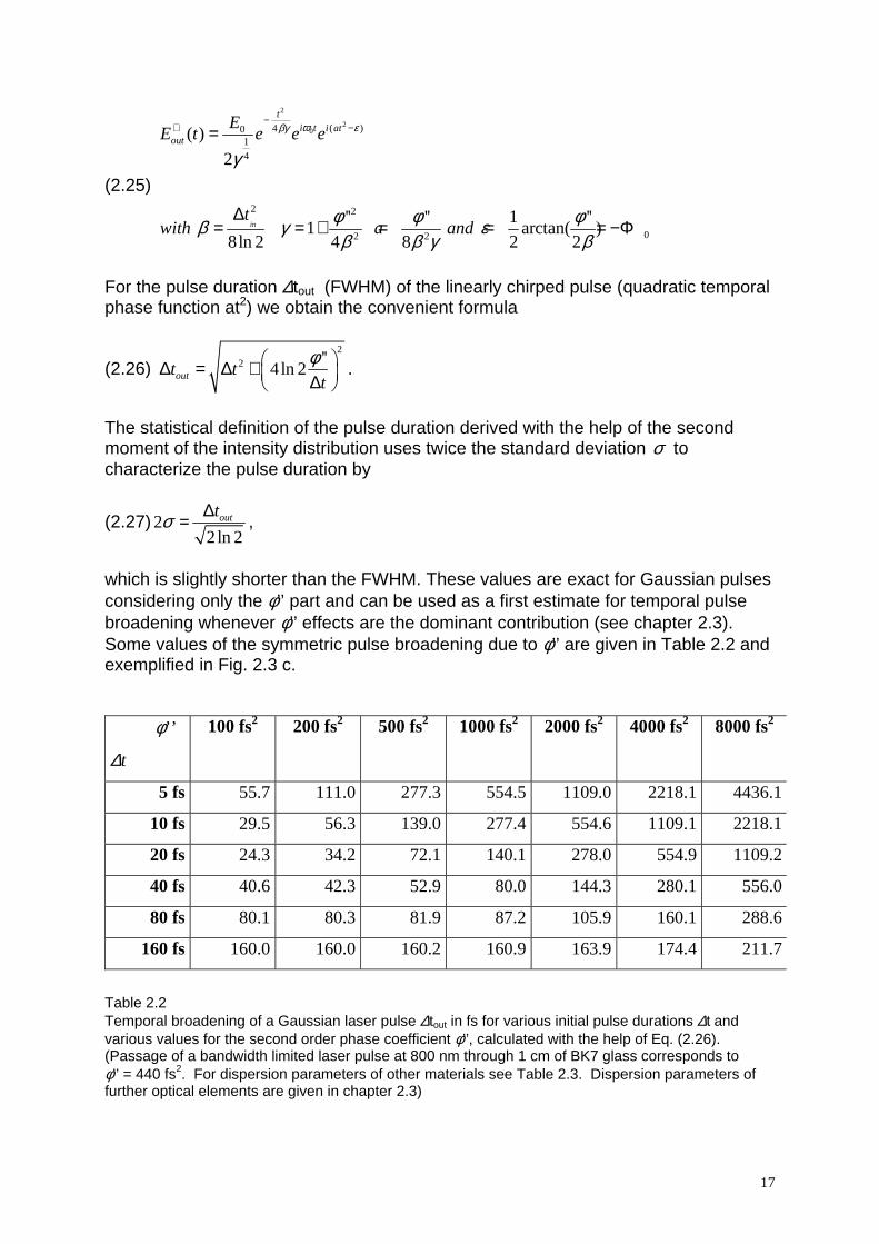
For the pulse duration ∆tout (FWHM) of the linearly chirped pulse (quadratic temporal phase function at2) we obtain the convenient formula
(2.26) 2
2 ''4 ln 2outt t
t
φ ∆ = ∆ + ∆ .
The statistical definition of the pulse duration derived with the help of the second moment of the intensity distribution uses twice the standard deviation σ to characterize the pulse duration by
(2.27) 22ln 2
outtσ ∆= ,
which is slightly shorter than the FWHM. These values are exact for Gaussian pulses considering only the φ’’ part and can be used as a first estimate for temporal pulse broadening whenever φ’’ effects are the dominant contribution (see chapter 2.3). Some values of the symmetric pulse broadening due to φ’’ are given in Table 2.2 and exemplified in Fig. 2.3 c. φ’’
∆t
100 fs2 200 fs2 500 fs2 1000 fs2 2000 fs2 4000 fs2 8000 fs2
5 fs 55.7 111.0 277.3 554.5 1109.0 2218.1 4436.1
10 fs 29.5 56.3 139.0 277.4 554.6 1109.1 2218.1
20 fs 24.3 34.2 72.1 140.1 278.0 554.9 1109.2
40 fs 40.6 42.3 52.9 80.0 144.3 280.1 556.0
80 fs 80.1 80.3 81.9 87.2 105.9 160.1 288.6
160 fs 160.0 160.0 160.2 160.9 163.9 174.4 211.7
Table 2.2 Temporal broadening of a Gaussian laser pulse ∆tout in fs for various initial pulse durations ∆t and various values for the second order phase coefficient φ’’, calculated with the help of Eq. (2.26). (Passage of a bandwidth limited laser pulse at 800 nm through 1 cm of BK7 glass corresponds to φ’’ = 440 fs2. For dispersion parameters of other materials see Table 2.3. Dispersion parameters of further optical elements are given in chapter 2.3)

18
Spectral phase coefficients of third order, i.e. a contribution to the phase function φ(ω)
of the form 30 0
1'''( ) ( )
6φ ω ω ω⋅ − are referred to as Third Order Dispersion (TOD). TOD
applied to the spectrum given by Eq. (2.28) yields the phase modulated spectrum
(2.29)2
2 31( ) '''( ) ( )
0 8ln 2 6( )2 2 ln 2
o o ot
i
out
E tE e e
ω ω φ ω ω ωπω∆− − − ⋅ −+ ∆=�
and leads to asymmetric temporal pulse shapes (McMullen, 1977) of the form
(2.30)
1/ 2 0
2ln 2 320
0
4 33 23
0 0 1/ 23 2
( ) ( )2 2ln 2
'''2(ln 2) ''' ( ''')
2 16
t
i tout
E t tE t Ai e e
twith sign and
t
τ
τ ωπ ττ τ
φ φτ φ φ τ τ φ τ τφ
−− ⋅
+ ∆ −=∆
∆= = ∆ = = =∆
where Ai describes the Airy function. Eq. (2.30) shows that the temporal pulse shape is given by the product of an exponential decay with a half-life period of 1/ 2τ and the Airy function shifted by τ and stretched by τ∆ . Fig. 2.3 d shows an example of a pulse subjected to TOD. The pulse shape is characterized by a strong initial pulse followed by a decaying pulse sequence. Because TOD leads to a quadratic group delay the central frequency of the pulse arrives first, while frequencies on either side arrive later. The two corresponding slightly differences in frequencies cause beats in the temporal intensity profile explaining the oscillations after (or before) the main pulse. The beating is also responsible for the phase jumps of π which occur at the zeros of the Airy function. Most of the relevant properties of TOD modulation are
determined by the parameter τ∆ which is proportional to 3 '''φ . The ratio of / tτ∆ ∆
determines whether the pulse is significantly modulated. If / 1tτ∆ ∆ ≥ , a series of
sub-pulses and phase jumps are observed. The sign of '''φ controls the time direction of the pulse shape: a positive value of '''φ leads to a series of post-pulses as shown in Fig. 2.3 d whereas negative values of '''φ cause a series of pre-pulses. The time shift of the most intense sub-pulse with respect to the unmodulated pulse and the FWHM of the sub-pulses are in the order of τ∆ . For these highly asymmetric pulses, the FWHM is not a meaningful quantity to characterize the pulse duration. Instead, the statistical definition of the pulse duration yields a formula similar to (2.26)
(2.31)22
22
'''2 8(ln 2)
2 ln 2
t
t
φσ ∆ = + ∆ .
It is a general feature of polynomial phase modulation functions, that the statistical pulse duration of a modulated pulse is
(2.32) 2 21 22σ τ τ= + ,

19
where 12ln 2
tτ ∆= is the statistical duration of the unmodulated pulse (cf. Eq. (2.27))
and ( )
2 1−∝∆
n
nt
φτ a contribution only dependent on the nth order spectral phase
coefficient. As a consequence, for strongly modulated pulses, when 2 1τ τ� , the
statistical pulse duration increases approximately linearly with ( )nφ . It is not always advantageous to expand the phase function φ(ω) into a Taylor series. Periodic phase functions, for example, are generally not well approximated by polynomial functions. For sinusoidal phase functions of the form
( ) ( )0sinAφ ω ω ϕ= ϒ + analytic solutions for the temporal electric field can be found for
any arbitrary unmodulated spectrum ( )inE ω+� . To this end we consider the modulated spectrum (2.33) ( )0sin( ) ( ) i A
out inE E e ω ϕω ω − ϒ++ +=� � , where Adescribes the amplitude of the sinusoidal modulation, ϒ the frequency of the modulation function (in units of time) and 0ϕ the absolute phase of the sine function. Making use of the Jacobi-Anger identity
(2.34) ( )0 0sin( ) ( )A inn
n
e J A eω ϕ ω ϕ∞
− ϒ+ − ϒ+
=−∞
= ∑ ,
where ( )nJ A describes the Bessel function of the first kind and order n, we rewrite
the phase modulation function
(2.35) ( ) 0( )( ) inn
n
M J A e ω ϕω∞
− ϒ+
=−∞
= ∑�
to obtain its Fourier transform
(2.36) ( ) ( )0( ) inn
n
M t J A e n tϕ δ∞
−
=−∞
= ϒ −∑ ,
where ( )tδ describes the delta function. Since multiplication in frequency domain
corresponds to convolution in time domain, the modulated temporal electrical field ( )outE t+ is given by convolution of the unmodulated field ( )inE t+ with the Fourier
transform of the modulation function ( )M t , i.e. ( )( ) ( )out inE t E t M t+ += ∗ . Making use of
Eq. (2.36) the modulated field reads
(2.37) ( ) 0( ) ( ) inout n in
n
E t J A E t n e ϕ∞
−+ +
=−∞
= − ϒ∑ .
Eq. (2.37) shows that sinusoidal phase modulation in frequency domain produces a sequence of sub-pulses with a temporal separation determined by the parameter ϒ
20
and well defined relative temporal phases controlled by the absolute phase 0ϕ . Provided the individual sub-pulses are temporally separated, i.e. ϒ is chosen to exceed the pulse width, the envelope of each sub-pulse is a (scaled) replica of the unmodulated pulse envelope. The amplitudes of the sub-pulses are given by ( )nJ A
and can therefore be controlled by the modulation parameter A . Examples of sinusoidal phase modulation are shown in Fig. 2.3 h-j. The influence of the absolute phase 0ϕ is depicted in Fig. 2.3 h and I, whereas Fig. 2.3 j shows how separated pulses are obtained by changing the modulation frequency ϒ . A detailed description of the effect of sinusoidal phase modulation can be found in (Wollenhaupt et al., 2006) 2.3 Changing the temporal shape via the frequency domain For the following discussion it is useful to think of an ultrashort pulse as being composed of groups of quasimonochromatic waves, that is of a set of much longer wave packets of narrow spectrum all added together coherently. In vacuum the
phase velocity v p k
ω= and the group velocity vg
d
dk
ω= are both constant and equal to
the speed of light c, where k denotes the wave number. Therefore an ultrashort pulse - no matter how complicated its temporal electric field is - will maintain its shape upon propagation in vacuum. In the following we will always consider a bandwidth limited pulse entering an optical system like for example air, lenses, mirrors, prisms, gratings etc. and combinations of these optical elements. Usually these optical systems will introduce dispersion, that is a different group velocity for each group of quasimonochromatic waves and consequently the initial short pulse will broaden in time. In this context the group delay Tg(ω) defined in Eq. (2.18) is the transit time for such a group of monochromatic waves through the system. As long as the intensities are kept low, no new frequencies are generated. This is the area of linear optics and the corresponding pulse propagation has been termed linear pulse propagation. It is convenient to describe the passage of an ultrashort pulse through a linear optical system by a complex optical transfer function (Diels and Rudolph, 1996) (Walmsley et al., 2001) (Weiner, 1995) (2.38) ( ) ( ) diM R e φω ω −=� � , that relates the incident electric field ( )inE ω+� with the output field (2.39) ( ) ( ) ( ) ( ) ( )di
out in inE M E R e Eφω ω ω ω ω−+ + += =� � � � � , where ( )R ω� is the real valued spectral amplitude response describing for example the variable diffraction efficiency of a grating, linear gain or loss or direct amplitude manipulation. The phase φd(ω) is termed the spectral phase transfer function. This is the phase accumulated by the spectral component of the pulse at frequency ω upon propagation between the input and output planes that define the optical system. It is this spectral phase transfer function that plays a crucial role in the design of ultrafast optical systems. Note that this approach is more involved when additional spatial coordinates have to be taken into account as for example in the case of “spatial chirp” (i.e. each frequency is displaced in the transverse spatial coordinates).

21
Neglecting spatial chirp this approach can be taken as a first order analysis of ultrafast optical systems. Although inside an optical system this condition might not be met, usually at the input and output all frequencies are assumed to be spatially overlapped for this kind of analysis. Note also that the “independence” of the different spectral components in this picture does not mean that the phase relations are random – they are uniquely defined with respect to each other. That means that the corresponding pulse in the time domain (by making use of Eq. (2.11) and (2.13)) is completely coherent (Meystre and Sargent III, 1998) no matter how complicated the shaped femtosecond laser pulse looks like. In the first order autocorrelation function a coherence time of the corresponding bandwidth limited pulse would be observed. Only in the higher order autocorrelations the uniquely defined phase relations show up (examples of second order autocorrelations for phase and amplitude shaped laser pulses are given in Fig. 4.5). Fig. 2.3 f-j exemplifies the temporal intensity, spectral intensity and related phase functions for often employed phase functions. Fig. 2.3 k-m displays the same quantities for amplitude modulation. Fig. 2.3 n is an example for self phase modulation and Fig. 2.3 o shows a double pulse with pulse to pulse delay of 60 fs. In the following discussion we will concentrate mainly on pure phase modulation and therefore set ( )R ω� constant for all frequencies and omit it initially. In order to model the system the most accurate way is to include the whole spectral phase transfer function. Often however only the first orders of a Taylor expansion around the central frequency ω0 are needed.
(2.40) 2 30 0 0 0 0 0 0
1 1( ) ( ) '( ) ( ) ''( ) ( ) '''( ) ( ) ...
2 6d d d d dφ ω φ ω φ ω ω ω φ ω ω ω φ ω ω ω= + ⋅ − + ⋅ − + ⋅ − +
If we describe the incident bandwidth limited pulse by
0 0 0( ) '( )( )( ) ( ) i iinE E e eφ ω φ ω ω ωω ω − − −+ +=� � then the overall phase φop of ( )outE ω+� is given by
(2.41)0 0 0 0 0 0
2 30 0 0 0
( ) ( ) '( ) ( ) ( ) '( ) ( )
1 1''( ) ( ) '''( ) ( ) ...
2 6
op d d
d d
φ ω φ ω φ ω ω ω φ ω φ ω ω ω
φ ω ω ω φ ω ω ω
= + ⋅ − + + ⋅ −
+ ⋅ − + ⋅ − +
As discussed in the context with Eq. (2.19) the constant and linear terms do not lead to a change of the temporal envelope of the pulse. Therefore we will omit in the following these terms and concentrate mainly on the second order dispersion φ’’ (also termed group velocity dispersion (GVD) or group delay dispersion (GDD)) and the third order dispersion φ’’’ (TOD) whereas we have omitted the subscript “d”. Strictly they have units of [fs2/rad] and [fs3/rad2] respectively but usually the units are simplified to [fs2] and [fs3]. A main topic in the design of ultrafast laser systems is to minimize these higher dispersion terms with the help of suitable designed optical systems in order to keep the pulse duration inside a laser cavity or at the place of an experiment as short as possible. In the following we will discuss the elements that are commonly used for the “dispersion management”. 2.3.1 Dispersion due to transparent media A pulse traveling a distance L through a medium with index of refraction n(ω) accumulates the spectral phase

22
(2.42) ( ) ( ) ( )m k L n Lc
ωφ ω ω ω= = ,
which is the spectral transfer function due to propagation in the medium as defined above. The first derivative
(2.43) 1
( )'
vm
m gg
d d kL d LL T
d d dk
φ ωφω ω
− = = = = =
yields the group delay Tg and describes the delay of the peak of the envelope of the incident pulse. Usually the index of refraction n(ω) is given as a function of wavelength λ, i.e. n(λ). Eq. (2.43) then reads
(2.44) ( ) ( )mg
d L dn L dnT n n
d c d c d
φ ω λω ω λ
= = + = − .
23
material λ [nm]
( )n λ
2 110
dn
d µmλ−
i 2
12 2
110
d n
d µmλ−
i 3
3 3
1dn
d µmλ
g
fsT
mm
2fsGDD
mm
3fs
TODmm
400 1,5308 -13,17 10,66 -12,21 5282 120,79 40,57
500 1,5214 -6,58 3,92 -3,46 5185 86,87 32,34 600 1,5163 -3,91 1,77 -1,29 5136 67,52 29,70
800 1,5108 -1,97 0,48 -0,29 5092 43,96 31,90
1000 1,5075 -1,40 0,15 -0,09 5075 26,93 42,88
BK7
1200 1,5049 -1,23 0,03 -0,04 5069 10,43 66,12
400 1,7783 -52,02 59,44 -101,56 6626 673,68 548,50
500 1,7432 -20,89 15,55 -16,81 6163 344,19 219,81 600 1,7267 -11,00 6,12 -4,98 5980 233,91 140,82
800 1,7112 -4,55 1,58 -0,91 5830 143,38 97,26
1000 1,7038 -2,62 0,56 -0,27 5771 99,42 92,79
SF10
1200 1,6992 -1,88 0,22 -0,10 5743 68,59 107,51
400 1,7866 -17,20 13,55 -15,05 6189 153,62 47,03
500 1,7743 -8,72 5,10 -4,42 6064 112,98 39,98 600 1,7676 -5,23 2,32 -1,68 6001 88,65 37,97
800 1,7602 -2,68 0,64 -0,38 5943 58,00 42,19
1000 1,7557 -1,92 0,20 -0,12 5921 35,33 57,22
Sapphire
1200 1,7522 -1,70 0,04 -0,05 5913 13,40 87,30
300 1,4878 -30,04 34,31 -54,66 5263 164,06 46,49
400 1,4701 -11,70 9,20 -10,17 5060 104,31 31,49 500 1,4623 -5,93 3,48 -3,00 4977 77,04 26,88
600 1,4580 -3,55 1,59 -1,14 4934 60,66 25,59
800 1,4533 -1,80 0,44 -0,26 4896 40,00 28,43 1000 1,4504 -1,27 0,14 -0,08 4880 24,71 38,73
Quartz
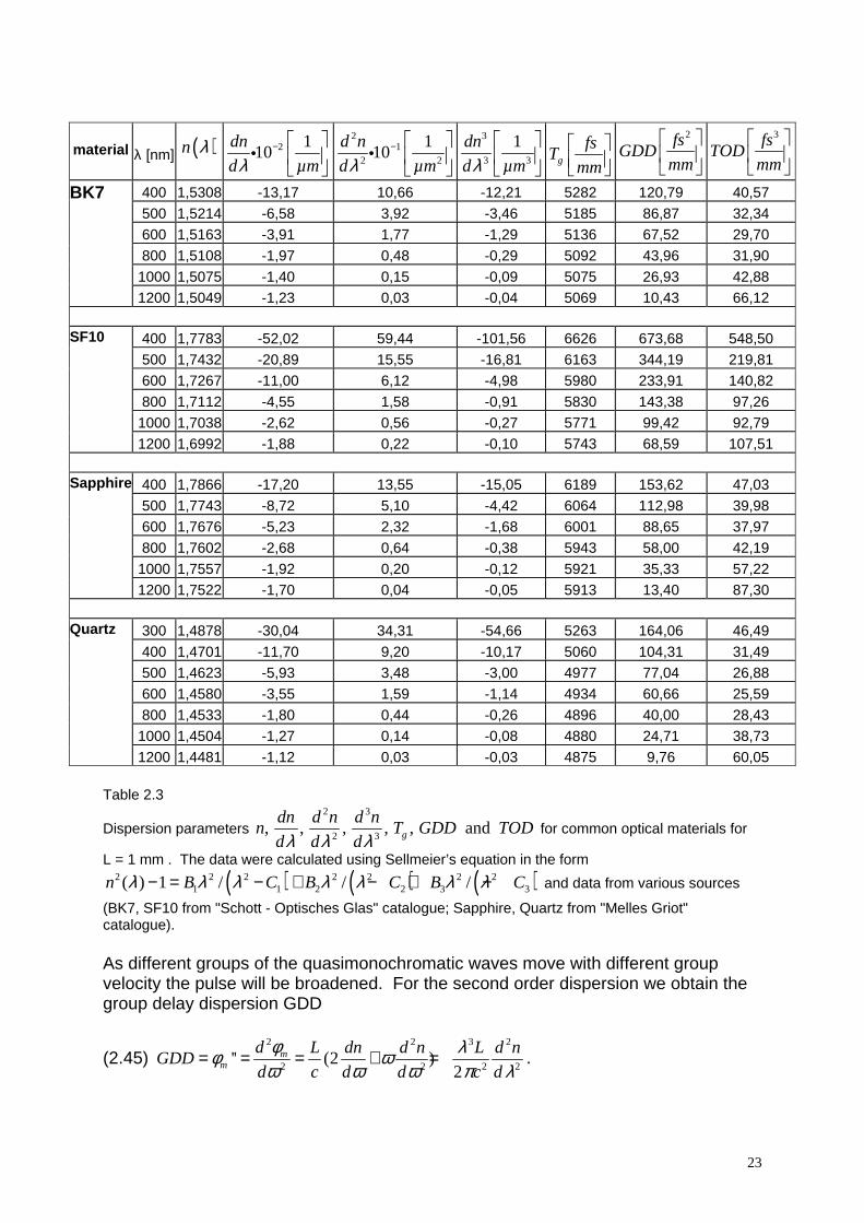
1200 1,4481 -1,12 0,03 -0,03 4875 9,76 60,05 Table 2.3
Dispersion parameters 2 3
2 3, , , , , andg
dn d n d nn T GDD TOD
d d dλ λ λ for common optical materials for
L = 1 mm . The data were calculated using Sellmeier’s equation in the form
( ) ( ) ( )2 2 2 2 2 2 21 1 2 2 3 3( ) 1 / / /n B C B C B Cλ λ λ λ λ λ λ− = − + − + − and data from various sources
(BK7, SF10 from "Schott - Optisches Glas" catalogue; Sapphire, Quartz from "Melles Griot" catalogue). As different groups of the quasimonochromatic waves move with different group velocity the pulse will be broadened. For the second order dispersion we obtain the group delay dispersion GDD
(2.45) 2 2 3 2
2 2 2 2'' (2 )
2m
m
d L dn d n L d nGDD
d c d d c d
φ λφ ωω ω ω π λ
= = = + = .

24
For ordinary optical glasses in the visible range we encounter normal dispersion i.e “red” parts of the laser pulse will travel “faster” through the medium than “blue” parts. So the symmetric temporal broadening of the pulse due to φ’’ will lead to a linearly up chirped laser pulse as discussed in the context of Eq. (2.19) and in Fig. 2.3 c. In these cases the curvature of n(λ) is positive (upward concavity) emphasizing the terminology that positive GDD leads to up-chirped pulses. For the third order dispersion TOD we obtain
(2.46) 3 2 3 4 2 3
3 2 3 2 3 2 3''' (3 ) (3 )
4m
m
d L d n d n L d n d nTOD
d c d d c d d
φ λφ ω λω ω ω π λ λ
−= = = + = + .
Empirical formulas for n(λ) such as Sellmeier's equations are usually tabulated for common optical materials so that all dispersion quantities in Eq. (2.44) to (2.46) can be calculated. Parameters for some optical materials are given in Table 2.3 for L = 1 mm. Note that in fiber optics a slightly other terminology is used (Walmsley et al., 2001). There the second order dispersion is the dominant contribution to pulse broadening. The β parameter of a fiber is related to the second order dispersion by
(2.47) 0
2
2 2
md
d ps
L kmω
φω
β =
,
where L denotes the length of the fiber and ps = picosecond. The dispersion parameter D is a measure for the group delay dispersion per unit bandwidth and given by
(2.48) 2
0
2
psD
c nm km
ω βπ
=
.
2.3.2 Angular dispersion Transparent media in the optical domain possess positive group delay dispersion leading to up chirped femtosecond pulses. In order to compress these pulses, optical systems are needed that deliver negative group delay dispersion, that is systems where the “blue” spectral components travel faster than the “red” spectral components. Convenient devices for that purpose are based on angular dispersion delivered by prisms and gratings. We start our discussion again with the spectral transfer function (Diels and Rudolph, 1996)
(2.49) ( ) ( )opPc
ωφ ω ω= ,
where Pop denotes the optical pathlength. Eq. (2.49) is the generalization of Eq. (2.42). The group delay dispersion is given by

25
Figure 2.4 Prism sequences for adjustable group delay dispersion. a) two prisms sequence in double pass configuration b) four prisms sequence. Note that the spatial distribution of the frequency (spatial chirp) after the second prism can be exploited for phase and / or amplitude manipulations.
(2.50) 2 22 3
2 2 2 2
12
2
= + =
op op opdP d P d Pd
d c d d c d
φ λωω ω ω π λ
and is similar to Eq. (2.45). In a dispersive system the optical path from an input reference plane to an output reference plane can be written by (2.51) cosopP l α= ,
where l=l(ω0) is the distance from the input plane to the output plane for the center frequency ω0 and α is the angle of rays with frequency ω with respect to the ray corresponding to ω0. In general, it can be shown (Diels and Rudolph, 1996) that the angular dispersion produces negative group delay dispersion
(2.52) 0
22
02
ld d
d c d ω
ωφ αω ω
≈ −
For pairs of elements (prisms or gratings) the first element provides the angular dispersion and the second element recollimates the spectral components (see for example Fig. 2.4). Using two pairs of elements permits the lateral displacement of
(b)
up chirp
down chirp
no chirp
l = l( )p 0ω
(a)
time

26
the spectral components (spatial chirp) to be cancelled out and recovers the original beam profile. 2.3.2.1 Prism sequences Prism pairs (Fork et al., 1984) are well suited to introduce adjustable group delay dispersion (see Fig. 2.4). Negative group delay dispersion is obtained via the angular dispersion of the first prism where the second prism is recollimating the beam. Recovering the original beam can be accomplished by either using a second pair of prisms or by using a mirror. Inside a laser cavity either the four prisms arrangement can be used or the two prisms arrangement for linear cavities together with a retroreflecting mirror. Outside a laser cavity often the two prism arrangement is used, where the retroreflecting mirror is slightly off axis in order to translate the recovered beam at the entrance of the system to be picked of by an additional mirror. There is also positive group delay dispersion in the system due to the material dispersion of the actual glass path the laser beam takes through the prism sequence. By translating one of the prisms along its axis of symmetry it is possible to change the amount of glass and therefore the amount of positive group delay dispersion. These devices allow a convenient continuous tuning of group delay dispersion from negative to positive values without beam deviation. The negative group delay dispersion via the angular dispersion can be calculated with the help of Eq. (2.49) and (2.51). In the case of minimum deviation and with the apex angle chosen so that the Brewster condition is satisfied (minimum reflection losses), the spectra phase introduced by a four prism sequence ( )pφ ω can be used to approximate the group
delay dispersion by (Diels and Rudolph, 1996)
(2.53) 22 3
2 2
4p pd l dn
d c d
φ λω π λ
≈ −
and the corresponding third order dispersion yields approximated
(2.54) 3 4 2
3 2 3 2
6p pd l dn dn d n
d c d d d
φ λλ
ω π λ λ λ
≈ +
.
In order to determine the total GDD and TOD of the four prism sequence the corresponding contributions of the cumulative mean glass path L (see Eq. (2.45) and (2.46)) have to be added
(2.55) 22 2 32 3 2
2 2 2 2 2 2
4
2fourprisms p pm
d d ld L d n dn
d d d c d c d
φ φ λφ λω ω ω π λ π λ
≈ + = −
(2.56)3 3 43 4 2 3 2
3 3 3 2 3 2 3 2 3 2
6(3 )
4fourprisms p pm
d d ld L d n d n dn dn d n
d d d c d d c d d d
φ φ λφ λ λ λω ω ω π λ λ π λ λ λ
−≈ + = + + +
.
For a more detailed discussion and other approaches for deriving the total GDD and TOD for a prism sequence see for example (Fork et al., 1984;Martinez et al., 1984;Duarte, 1987;Petrov et al., 1988;Barty et al., 1994).
27
In principle one can get any amount of negative group velocity using this method. However a prism distance exceeding 1 m is often impractical. Higher amounts of positive group delay dispersion might be compensated for by the use of highly dispersive SF10 prisms but the relatively higher third order contribution prevent the generation of ultrashort pulses in the 10 fs regime. Fused quartz is a suited material for ultrashort pulse generation with minimal higher order dispersion. For example a four prisms sequence with lp = 50 cm of fused quartz used at 800 nm yields roughly
22
21000pd
fsd
φω
≈ − . Estimating a cumulative glass path of L = 8 mm when going
through the apexes of the prisms yields 2
22
300mdfs
d
φω
≈ . In this way a maximum group
delay dispersion of +700 fs2 can be compensated. Note that in such prism sequences the spatial distribution of the frequency components after the second prism can be exploited. Simple apertures can be used to tune the laser or to restrict the bandwidth. Appropriate phase or amplitude masks might be inserted as well. 2.3.2.2 Grating arrangements Diffraction gratings provide group delay dispersion in a similar manner to prisms. Suitable arrangements can introduce positive as well as negative group delay dispersion (see below). When introducing negative group delay dispersion the corresponding device is termed a "compressor", while a device introducing positive group delay dispersion is termed a “stretcher”. Grating arrangements have the advantage to be much more dispersive but the disadvantage to introduce higher losses than prism arrangements. Intracavity they are used for example in high gain fiber lasers. Outside laser cavities they are widely used
• to compensate for large amounts of dispersion in optical fibers • for ultrashort pulse amplification up to the Petawatt regime with a technique
called Chirped Pulse Amplification (CPA) (Strickland and Mourou, 1985): In order to avoid damage to the optics and to avoid nonlinear distortion to the spatial and temporal profile of the laser beam, ultrashort pulses (10 fs to 1 ps) are typically stretched in time by a factor of 103-104 prior to the injection into the amplifier. After the amplification process the pulses have to be recompressed compensating also for additional phase accumulated during the amplification process. The topic is reviewed in (Backus et al., 1998).
• for pulse shaping applications (see chapter 2.3.4). • in combination with prism compressors to compensate third order dispersion
terms in addition to the group delay dispersion (Cruz et al., 1988). This was the combination employed to establish the long standing world record of 6 fs with dye lasers in 1987 (Fork et al., 1987).
In Fig. 2.5 the reflection of a laser beam from a grating is displayed. The spectrum of an ultrashort laser pulse will be decomposed after reflection into the first order according to the grating Eq.
(2.57) ( ) ( )d
sinsinλθγ =+ ,
where γ is the angle of incidence, θ is the angle of the reflected wavelength component and d-1 is the grating constant. Blazed diffraction gratings have maximum

28
Figure 2.5 Reflection from a grating: the spectrum of an ultrashort laser pulse will be decomposed after reflection (γ = angle of incidence, θ(λ) = angle of reflection, d-1 = grating constant). transmission efficiency when employed in Littrow configuration, i.e. γ = θ(λ0) =blaze angle. This has the additional advantage that astigmatism is minimized. Blazed gold gratings with an efficiency of 90% to 95% are commercially available with a damage threshold of >250 mJ/cm2 for a 1 ps pulse. For higher efficiency and higher damage threshold dielectric gratings are developed. For example dielectric gratings with 98% efficiency at 1053 nm and a damage threshold >500mJ/cm2 for fs pulses are available. A basic grating compressor (see Fig. 2.6) consists of two parallel gratings in double pass configuration (Treacy, 1969). The first grating decomposes the ultrashort laser pulse into its spectral components. The second grating is recollimating the beam. The original beam is recovered by use of a mirror that inverts the beam. As in such a device the “red” spectral components experience a longer optical path compared to the “blue” spectral components, such an arrangement is suited to compensate for material
dispersion. In Fig. 2.7 different grating configurations are displayed that produce (a) zero, (b) positive and (c) negative group delay dispersion. Between the gratings an additional telescope is employed.
γ Θ λ( )
d
l0
lg
γ
Θλ(
)0
blue
red
Figure 2.6 Grating compressor with parallel gratings and a mirror for beam inversion (compare to the corresponding prism set up in Fig. 2.4a). The “red” spectral components travel a longer optical path compared to the “blue” spectral components (lg denotes the distance between the grating; l0 denotes the optical path for the centre wavelength λ0 between two gratings; both lengths are used by different authors in deriving the group delay dispersion and the third order dispersion).

29
Figure 2.7 Different grating configurations that produce (a) zero, (b) positive and (c) negative group delay dispersion. Arrangement (a) corresponds to a zero dispersion compressor, (b) to a stretcher and (c) to a compressor. The zero dispersion compressor is often used in pulse shaping devices (the dashed line in (a) indicates the Fourier transform plane, whereas the stretcher and compressor are key components for chirped pulse amplification. In Fig. 2.7 a) a so called zero dispersion compressor is depicted. The system consists of a telescope that images the laser spot on the first grating onto the second grating. All wavelength components experience the same optical path. In this manner zero net dispersion is obtained. Due to the finite beam size on the grating the components belonging to the same wavelength emerge as a parallel beam and are focused with the lens of focal length f spectrally into the symmetry plane thus providing a Fourier transform plane for pulse shaping, masking or encoding (see chapter 2.3.4 and Fig. 2.11). Translating one of the gratings out of the focal plane closer to the telescope (see Fig. 2.7 b) results in an arrangement where the red components travel a shorter optical path. The device introduces positive group delay dispersion (stretcher).
f f
f
red
blue
2f
a=0
a)
red
bluea>0
c)
f
f
f
red
blue
2f
2f
lt
l t
a<0
b)
30
A compressor is realized by translating the grating away from the focal plane. (see Fig. 2.7c). The dispersion can be further modified by the use of a magnifying telescope. In order to avoid material dispersion in the lenses and to minimize aberration effects, reflective telescopes and especially Öffner telescopes are usually employed (Suzuki, 1983;Cheriaux et al., 1996). The phase transfer function gφ for these arrangements can be calculated with the
help of a matrix formalism (Martinez, 1988) and considering the case of finite beam size (Martinez, 1986). For a reflective set up (neglecting material dispersion) the group delay dispersion and the third order dispersion of the three telescope arrangements (magnification=1) in Fig. 2.7 can be described using a characteristic length L
(2.58) ( )( )
2 3
22 2 2
1
cos
gdL
d c d
φ λω π θ λ
= −
(2.59) ( )( )( )( )
3 2
3 2
tan31
2 cosg gd d
d d c d
θ λφ φ λ λω ω π θ λ
= +
With the help of the grating Eq. (2.57) cos(θ(λ)) is given by:
(2.60) ( )( )2
1
−−= γλλθ sind
cos
In reflective telescope setups usually only one grating is employed using suitable beam folding arrangements. This reflects the situation when both gratings in Fig. 2.7 are moved out of the focal plane symmetrically. For the telescope arrangements we therefore obtain as characteristic length L= 2 f a. According to Fig. 2.7 the parameter a is determined by the distance of the grating to the lens
(2.61)
: , 0
1 : , 0
: , 0
t
tt
t
Compressor l f al
a Zero dispersion compressor l f af
Stretcher l f a
> >= − = = < <
For the grating compressor depicted in Fig. 2.6 the characteristic length L is given by
(2.62)
( )0 2
l
1 sin
gL l
d
λ γ
= = − −
,
where l0 is the optical pathlength of the centre wavelength λ0 between the gratings and lg is the distance of the gratings. For the compressor in Fig. 2.6 we obtain a group delay dispersion of -1 106 fs2 (λ = 800 nm, d-1 = 1200l/mm, l0 = 300 mm; γ = 28,6o (Littrow)) being orders of magnitude higher than the example given for the prism sequence (see chapter 2.3.2.1).
31
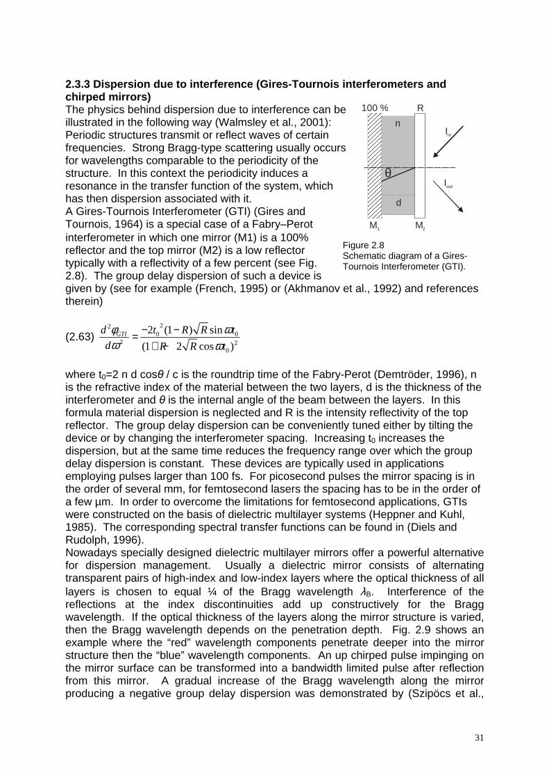
2.3.3 Dispersion due to interference (Gires-Tournois interferometers and chirped mirrors) The physics behind dispersion due to interference can be illustrated in the following way (Walmsley et al., 2001): Periodic structures transmit or reflect waves of certain frequencies. Strong Bragg-type scattering usually occurs for wavelengths comparable to the periodicity of the structure. In this context the periodicity induces a resonance in the transfer function of the system, which has then dispersion associated with it. A Gires-Tournois Interferometer (GTI) (Gires and Tournois, 1964) is a special case of a Fabry–Perot interferometer in which one mirror (M1) is a 100% reflector and the top mirror (M2) is a low reflector typically with a reflectivity of a few percent (see Fig. 2.8). The group delay dispersion of such a device is given by (see for example (French, 1995) or (Akhmanov et al., 1992) and references therein)
(2.63) 22
0 02 2
0
2 (1 ) sin
(1 2 cos )GTId t R R t
d R R t
φ ωω ω
− −=+ −
where t0=2 n d cosθ / c is the roundtrip time of the Fabry-Perot (Demtröder, 1996), n is the refractive index of the material between the two layers, d is the thickness of the interferometer and θ is the internal angle of the beam between the layers. In this formula material dispersion is neglected and R is the intensity reflectivity of the top reflector. The group delay dispersion can be conveniently tuned either by tilting the device or by changing the interferometer spacing. Increasing t0 increases the dispersion, but at the same time reduces the frequency range over which the group delay dispersion is constant. These devices are typically used in applications employing pulses larger than 100 fs. For picosecond pulses the mirror spacing is in the order of several mm, for femtosecond lasers the spacing has to be in the order of a few µm. In order to overcome the limitations for femtosecond applications, GTIs were constructed on the basis of dielectric multilayer systems (Heppner and Kuhl, 1985). The corresponding spectral transfer functions can be found in (Diels and Rudolph, 1996). Nowadays specially designed dielectric multilayer mirrors offer a powerful alternative for dispersion management. Usually a dielectric mirror consists of alternating transparent pairs of high-index and low-index layers where the optical thickness of all layers is chosen to equal ¼ of the Bragg wavelength λB. Interference of the reflections at the index discontinuities add up constructively for the Bragg wavelength. If the optical thickness of the layers along the mirror structure is varied, then the Bragg wavelength depends on the penetration depth. Fig. 2.9 shows an example where the “red” wavelength components penetrate deeper into the mirror structure then the “blue” wavelength components. An up chirped pulse impinging on the mirror surface can be transformed into a bandwidth limited pulse after reflection from this mirror. A gradual increase of the Bragg wavelength along the mirror producing a negative group delay dispersion was demonstrated by (Szipöcs et al.,
θ
n
d
M2M1
Iin
Iout
100 % R
Figure 2.8 Schematic diagram of a Gires- Tournois Interferometer (GTI).
32
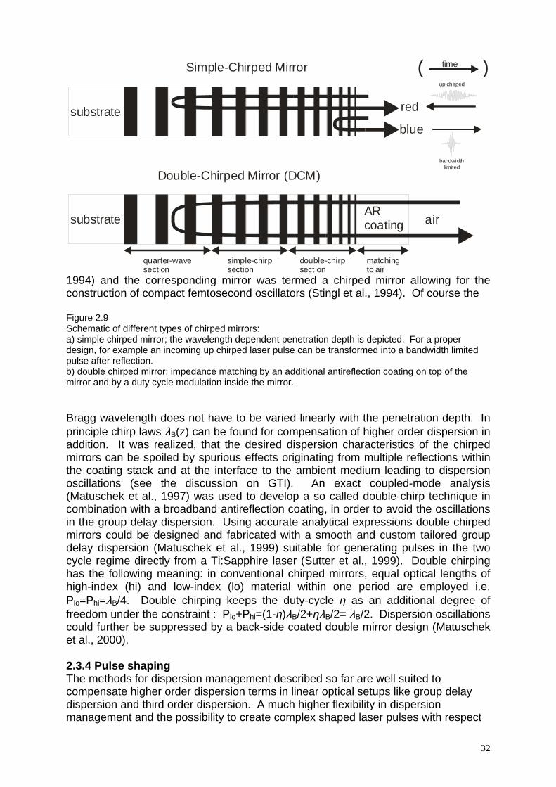
1994) and the corresponding mirror was termed a chirped mirror allowing for the construction of compact femtosecond oscillators (Stingl et al., 1994). Of course the Figure 2.9 Schematic of different types of chirped mirrors: a) simple chirped mirror; the wavelength dependent penetration depth is depicted. For a proper design, for example an incoming up chirped laser pulse can be transformed into a bandwidth limited pulse after reflection. b) double chirped mirror; impedance matching by an additional antireflection coating on top of the mirror and by a duty cycle modulation inside the mirror. Bragg wavelength does not have to be varied linearly with the penetration depth. In principle chirp laws λB(z) can be found for compensation of higher order dispersion in addition. It was realized, that the desired dispersion characteristics of the chirped mirrors can be spoiled by spurious effects originating from multiple reflections within the coating stack and at the interface to the ambient medium leading to dispersion oscillations (see the discussion on GTI). An exact coupled-mode analysis (Matuschek et al., 1997) was used to develop a so called double-chirp technique in combination with a broadband antireflection coating, in order to avoid the oscillations in the group delay dispersion. Using accurate analytical expressions double chirped mirrors could be designed and fabricated with a smooth and custom tailored group delay dispersion (Matuschek et al., 1999) suitable for generating pulses in the two cycle regime directly from a Ti:Sapphire laser (Sutter et al., 1999). Double chirping has the following meaning: in conventional chirped mirrors, equal optical lengths of high-index (hi) and low-index (lo) material within one period are employed i.e. Plo=Phi=λB/4. Double chirping keeps the duty-cycle η as an additional degree of freedom under the constraint : Plo+Phi=(1-η)λB/2+ηλB/2= λB/2. Dispersion oscillations could further be suppressed by a back-side coated double mirror design (Matuschek et al., 2000). 2.3.4 Pulse shaping The methods for dispersion management described so far are well suited to compensate higher order dispersion terms in linear optical setups like group delay dispersion and third order dispersion. A much higher flexibility in dispersion management and the possibility to create complex shaped laser pulses with respect
substrate
substrate red
blue
up chirped
bandwidth limited
Simple-Chirped Mirror
Double-Chirped Mirror (DCM)
ARcoating air
quarter-wavesection
simple-chirpsection
double-chirpsection
matchingto air
time( )

33
to phase, amplitude and polarization state is given with the help of (computer controlled) pulse shaping techniques (see Fig. 2.10 a)). The issue was recently reviewed by Weiner (Weiner, 1995) (Weiner, 2000).
PULSE SHAPER
a)
b)
feedbacksignal
calculated modifiedelectric fields
real electric fields
COMPUTERLEARNING
ALGORITHMPULSE SHAPER
EXPERIMENT
OBJECTIVE
Figure 2.10 a) Pulse shaping issues (schematic): Creation of bandwidth limited pulses from complex structured pulses (left to right). Creation of "tailored" pulse shapes (right to left). b) Adaptive femtosecond pulse shaping: A femtosecond laser system (not indicated) and a computer controlled pulse shaper are used to generate specific electric fields which are sent into an experiment. After deriving a suitable feedback signal from the experiment a learning algorithm calculates modified electric fields based on the information from the experimental feedback signal and the user defined control objective. The improved laser pulse shapes are tested and evaluated in the same manner. Cycling through this loop many times results in iteratively optimized laser pulse shapes that finally approach the objective.

34
A new class of experiments emerged in which pulse shaping techniques were combined with some experimental signal embedded in a feedback learning loop (Judson and Rabitz, 1992) (Baumert et al., 1997) (Bardeen et al., 1997) (Yelin et al., 1997): in this approach a given pulse shape is evaluated in order to produce an improved pulse shape which enhances the feedback signal (see Fig. 2.10 b)). These techniques have an impact on an increasing number of scientists in physics, chemistry, biology and engineering. This is due to the fact that primary light induced processes can be studied and even actively controlled via adaptive femtosecond pulse shaping. For a small selection of work in various areas see for example (Assion et al., 1998) (Brixner et al., 1999) (Bartels et al., 2000) (Brixner et al., 2001) (Herek et al., 2002) (Kunde et al., 2000) (Weinacht et al., 2001) (Levis et al., 2001) (Daniel et al., 2003) (Brixner and Gerber, 2003;Wollenhaupt et al., 2005b;Horn et al., 2006). Because of their short duration, femtosecond laser pulses cannot be directly shaped in the time domain. Therefore, the idea of pulse shaping is modulating the incident spectral electric field ( )inE ω+� by a linear mask, i.e. the optical transfer function, ( )M ω� in the frequency domain. According to Eq. (2.39) this results in an outgoing shaped spectral electric field ( ) ( ) ( ) ( ) ( )di
out in inE M E R e Eφω ω ω ω ω−+ + += =� � � � � . The mask may modulate
the spectral amplitude response ( )R ω� and the spectral phase transfer function ( )dφ ω . Furthermore, polarization shaping has been demonstrated (Brixner and Gerber, 2001).
f ff f
)(tEin )(tEout
)(~ ωinE ( )outE ω~
( )M ω~
blue
red
Figure 2.11 Basic layout for Fourier transform femtosecond pulse shaping. One way to realize a pulse shaper is the Fourier transform pulse shaper. Its operation principle is based on optical Fourier transformations from the time domain into the frequency domain and vice versa. In Fig. 2.11 a standard design of such a pulse shaper is sketched. The incoming ultrashort laser pulse is dispersed by a

35
grating and the spectral components are focused by a lens of focal length f. In the back focal plane of this lens - the Fourier plane - the spectral components of the original pulse are separated from each other having minimum beam waists. By this means, the spectral components can be modulated individually by placing a linear mask into the Fourier plane. Afterwards, the laser pulse is reconstructed by performing an inverse Fourier transformation back into the time domain. Optically, this is realized by a mirrored setup consisting of an identical lens and grating. The whole setup - without the linear mask - is called a zero-dispersion compressor since it introduces no dispersion if the 4 f condition is met (see also Fig. 2.7a)). As a part of such a zero-dispersion compressor, the lenses separated by the distance 2 f, form a telescope with unitary magnification. Spectral modulations as stated by Eq. (2.39) can be set by inserting the linear mask. Due to the damage threshold of the linear masks used, usually cylindrical focusing lenses (or mirrors) are used instead of spherical optics. The standard design in Fig. 2.11 has the advantage that all optical components are positioned along an optical line (grating in Littrow configuration). For ultrashort pulses below 100 fs, however, spatial and temporal reconstruction errors are becoming a problem due to the chromatic abberations introduced by the lenses. Therefore, lenses are often replaced by curved mirrors. In general, optical errors are minimized if the tilting angles of the curved mirrors within the telescope are as small as possible. A folded, compact and dispersion optimized set up is depicted in Fig. 2.12 (Präkelt et al., 2003). For ultrashort pulses in the <10 fs regime prisms have been employed as dispersive elements instead of gratings (Xu et al., 2000). A very popular linear mask for computer controlled pulse shaping in such set ups is the Liquid Crystal Spatial Light Modulator (LC-SLM). A schematic diagram of an electronically adressed phase only LC-SLM is depicted in Fig. 2.13. In the Fourier plane the individual wavelength components of the laser pulse are spatially dispersed and can be conveniently manipulated by applying voltages at the separate pixels leading to changes of the refractive index . Upon transmission of the laser beam through the LC-SLM a frequency-dependent phase is acquired due to the individual pixel voltage values and consequently the individual wavelength components are retarded with respect to each other. Actual LC-SLMs contain up to 640 pixels (Stobrawa et al., 2001). In this way, an immensely large number of different spectrally phase modulated pulses can be produced. A phase only LC-SLM does to a first approximation not change the spectral amplitudes and therefore the integrated pulse energy remains constant for different pulse shapes. By virtue of the Fourier transform properties, spectral phase
CM GFM
CM GFM
FP
Figure 2.12 Dispersion optimized layout for Fourier transform femtosecond pulse shaping. The incoming beam is dispersed by the first grating (G). The spectral components go slightly out of plane and are sagitally focused by a cylindrical mirror (CM) via a plane folding mirror (FM) in the Fourier plane (FP). Then the original beam is reconstructed by a mirrored set up.

36
changes result in phase- and amplitude-modulated laser pulse temporal profiles as depicted schematically in Fig. 2.14. If such a LC-SLM is oriented at 450 with respect to the linear polarization of the incident light field (either with the help of a wave plate or a suitable designed LC-SLM), polarization is induced in addition to retardance. A single LC-SLM together
with a polarizer can be used therefore as an amplitude modulator. However, this Figure 2.13 Schematic diagram of an electronically addressed phase only Liquid Crystal - Spatial Light Modulator (LC-SLM). By adjusting the voltages of the individual pixels, the liquid crystal molecules reorient themselves on average partially along the direction of the electric field. This leads to a change in refractive index and therefore to a phase modulation which can be independently controlled for different wavelength components.
electric ground (ITO)liquid crystalelectrodes (ITO)
gap (3 µm)
pixel (97 µm) voltage off
linear polarization
voltage on
light propagation

37
Figure 2.14 Schematic illustration of shaping the temporal profile of an ultrashort laser pulse by retardation of the spectrally dispersed individual wavelength components in a phase only LC-SLM. The LC-SLM is located in the Fourier plane of the set ups displayed in Fig. 2.11 and Fig. 2.12. leads also to phase modulation depending on the amplitude modulation level. For independent phase and amplitude control dual LC-SLMs are currently used. In such a set up a second LC-SLM is fixed back-to-back at -45° with respect to the linear polarization of light in front of the first LC-SLM and the stack is completed with a polarizer. For an early setup for independent phase and amplitude modulations see (Wefers and Nelson, 1993) whereas nowadays configurations are described in (Weiner, 2000). Alternatively, simple amplitude modulation functions ( )�R ω can be realized by insertion of absorbing material at specific locations in the Fourier plane thus eliminating the corresponding spectral components within the pulse spectrum (Präkelt et al., 2005). For polarization shaping (Brixner and Gerber, 2001) the polarizer is removed and spectral phase modulation can be imposed independently onto two orthogonal polarization directions. The interference of the resulting elliptically polarized spectral components leads to complex evolutions of the polarization state in the time domain. As any element between the LC-SLM stack and the experiment can modify the polarization evolution, dual-channel spectral interferometry and experimentally calibrated Jones-matrix analysis have been employed for characterization (Brixner et al., 2002). A representation of a complex polarization shaped pulse is displayed in Fig. 2.15. Such pulses open up an immense range of applications, especially in quantum control, because vectorial properties of multi photon transitions can be addressed (Brixner et al., 2004;Wollenhaupt et al., 2005a). Another possibility to realize phase only pulse shaping is based on deformable mirrors consisting of a small number (orders of ten) of electrostatic controlled membrane mirrors (Zeek et al., 1999). These devices are placed in the Fourier plane and by a slight out of plane tilt upon reflection half of the optics can be saved (see

38
Fig. 2.16 for an illustration). The use of a micro mirror array with 240 x 200 pixels used in reflection and a waveform update rate larger than 1 kHz was also demonstrated (Hacker et al., 2003). Acousto optic modulators (AOMs) can be used for programmable pulse shaping as well. There exist two different approaches. One approach is depicted in Fig. 2.17 and is reviewed in (Tull et al., 1997) and (Goswami, 2003). The AOM crystal is oriented at Bragg angle at the Fourier plane of a zero dispersion compressor. In the visible usually TeO2 crystals are used whereas in the infrared InP crystals are employed. A programmable radio frequency (RF) signal driving the piezoelectric transducer of the AOM creates an acoustic wave that propagates through the crystal. As light travels at orders of magnitude faster velocity, the acoustic wave can be considered as a fixed modulated grating at the moment the spatially dispersed laser beam hits the crystal. The amplitude and phase of the acoustic wave determine the diffraction efficiency and phase shift at each point in space. The beam is diffracted typically below 1° b y the AOM via the photoelastic effect. AOMs can place in the order of thousand independent features onto the spectrum and have a significantly faster update rate as compared to the LC-SLMs. On the other hand the optical throughput of such devices is well below 50% and typical modelocked laser sources running at 100 MHz repetition rate in general cannot be pulse shaped because the acoustic wave is travelling within 10 ns several ten µm. This is not a limitation for amplified ultrafast laser systems where the pulse repetition rate is usually slower than the acoustic aperture time, since this allows the acoustic pattern to be synchronized to each amplifier pulse and to be refreshed before the next pulse arrives. The other AOM approach is based on an acousto-optic programmable dispersive filter (AOPDF) and does not need to be placed in the Fourier plane of a 4f device (Tournois, 1997) (Verluise et al., 2000a) (Verluise et al., 2000b). A schematic of that device is shown in Fig. 2.18. Again, a programmable radio frequency (RF) signal driving the piezoelectric transducer of the AOM creates an acoustic wave that
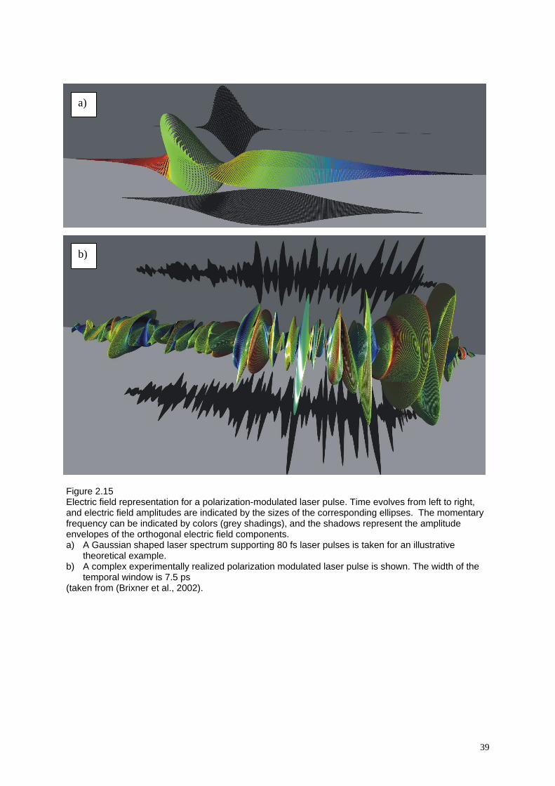
39
Figure 2.15 Electric field representation for a polarization-modulated laser pulse. Time evolves from left to right, and electric field amplitudes are indicated by the sizes of the corresponding ellipses. The momentary frequency can be indicated by colors (grey shadings), and the shadows represent the amplitude envelopes of the orthogonal electric field components. a) A Gaussian shaped laser spectrum supporting 80 fs laser pulses is taken for an illustrative
theoretical example. b) A complex experimentally realized polarization modulated laser pulse is shown. The width of the
temporal window is 7.5 ps (taken from (Brixner et al., 2002).
a)
b)

40
Figure 2.16 Schematic of a phase only deformable-mirror pulse shaper.
f
f
f
f
1°
RF arbitrary function generator(200 MHz, 90 MHz)
f
f
f
f
1°
RF arbitrary function generator(200 MHz, 90 MHz)
1°
RF arbitrary function generator(200 MHz, 90 MHz)
RF arbitrary function generator
Input pulse Ouput pulse Figure 2.17 Programmable pulse shaping device based on the use of an acousto optic modulator as the spatial light modulator.
Ein(t) (mode1)
Ein(t) Eout (t)E(mode2)
out (t)
AO transducerRF arbitrary RF arbitrary function generator
acoustic wave
birefringent crystal
f f
linear array of electrodes
silicon nitride membrane coated with gold
Figure 2.18 Schematic of an acousto-optic programmable dispersive filter (AOPDF).

41
propagates through the crystal and reproduces spatially the temporal shape of the RF signal. Two optical modes can be coupled efficiently by acousto optic interaction only in the case of phase matching. If there is locally only one spatial frequency in the acoustic grating, then only one optical frequency can be diffracted at that position from the fast ordinary axis (mode 1) to the slow extraordinary axis (mode 2). The incident optical short pulse is initially in mode 1. Different groups of optical frequency components travel a different distance before they encounter phase matched spatial frequencies in the acoustic grating. At that positions part of the energy is diffracted on mode 2. The pulse leaving the device at mode 2 will be made of all spectral components that have been diffracted at the various positions. If the velocities of the two modes are different, each frequency will see a different time delay. The amplitude of specific frequency components of the output pulse is controlled by the acoustic power at the position where that frequency components are diffracted. With the help of a 2.5 cm long TeO2 crystal, a group delay range of 3 ps, 6.7 fs temporal resolution and 30 % diffraction efficiency are reported (Verluise et al., 2000a). In general pulse shapers based on LC-SLM or on deformable mirrors have low transmission losses, are suitable also for high repetition rate mode-locked laser oscillators, do not impose additional chirp and have a low waveform update rate on the order of 10 Hz. Set ups based on AOMs have high transmission losses, they do impose additional chirp but they have a waveform update rate in the order of 100 kHz. Both AOMs and LC-SLMs can impose in the order of 1000 independent features onto the spectrum and both are suitable for amplitude and phase modulation. Programmable polarization shaping has been demonstrated so far only with LC-SLMs. The programmable femtosecond pulse shaping techniques described up to now allow control of the temporal profile of an output waveform in phase, amplitude and polarization. This can be thought of as control over one spatial dimension, the direction of propagation. With that respect this "temporal-only" pulse shaping is one dimensional. Automated two dimensional phase-only pulse shaping employing an optically addressed reflective two-dimensional SLM with negligible interpixel gaps allows real-space pulse shaping, in which a sample or device is irradiated with different temporally shaped waveforms at different locations (Vaughan et al., 2002). The pulse shaping arrangement is similar to conventional 4f spectral filtering arrangements, with the difference that the incoming beam is expanded in one dimension and the two dimensional SLM is employed in reflection geometry. Such a unit has been employed for two-dimensional shaping of surface polaritons (Feurer et al., 2003).

42
3. Generation of femtosecond laser pulses via mode locking Femtosecond laser pulses can be generated directly from a wide variety of lasers with wavelengths ranging from the ultraviolet to the infrared. This range is greatly extended by the use of nonlinear frequency conversion techniques. Continuous tuning is achieved for example via optical parametric oscillators followed by (cascaded) sum- and difference frequency mixing. Tuning of amplified femtosecond laser systems is achieved via optical parametric amplifiers. The generation of a white light continuum is also a standard technique to generate new wavelengths. With high power femtosecond laser systems the x-ray region can be reached by focusing the radiation into a solid state material or via high harmonic generation whereas the latter technique also opens the door to the attosecond regime. The THz spectral region can be accessed via femtosecond lasers as well. With very few exceptions the generation of ultrashort pulses relies on a technique termed mode locking. The topic has been covered in review articles (see for example (New, 1983) (Simon, 1989) (French, 1995) (French, 1996) (Haus, 2000)), in several books devoted to ultrashort laser pulses (see for example (Fleming, 1986) (Wilhelmi and Herrmann, 1987) (Akhmanov et al., 1992) (Diels and Rudolph, 1996) (Rulliere, 1998)) and in general laser text books (see for example (Svelto, 1998) (Siegmann, 1986) (Yariv, 1989) (Demtröder, 1996)). For a recent compilation of mode locking different laser systems ranging from solid state lasers over fiber lasers to semiconductor lasers see for example (Fermann et al., 2003). Here we will limit the description to the basic concepts of mode locking.
Figure 3.1 Simple snapshot representation of a mode locked laser. The pulse P is propagating back and forth between the end mirror EM and the output coupler OC. The pulses in the output beam are separated by 2L in space (or 2L/c=TRT in time). The dashed box represents the gain medium and other laser components. A laser is typically constructed with a pair of mirrors separated by a distance L which enclose a gain medium and other components. In a continuously operating (cw) laser or in a pulsed laser where the pulse duration is substantially greater then the cavity round trip time TRT
(3.1) 2
RT
LT
c=
EM OC
L
2 L 2 L
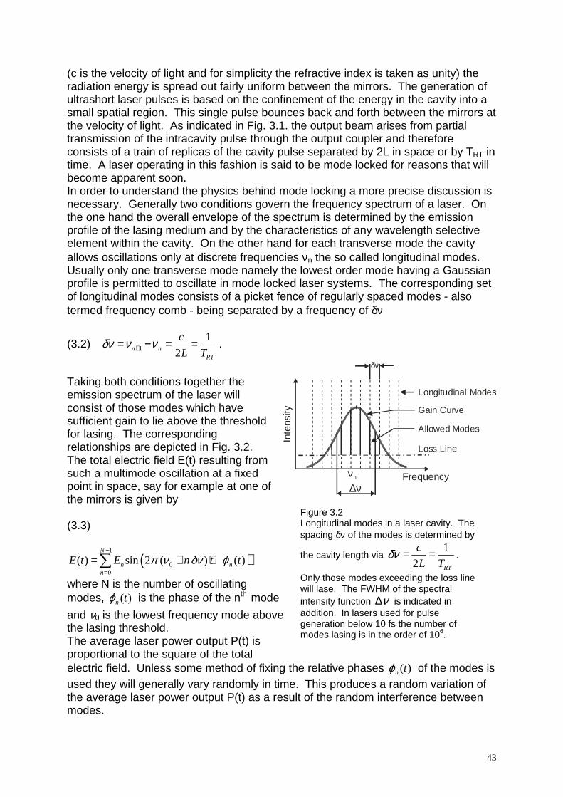
43
(c is the velocity of light and for simplicity the refractive index is taken as unity) the radiation energy is spread out fairly uniform between the mirrors. The generation of ultrashort laser pulses is based on the confinement of the energy in the cavity into a small spatial region. This single pulse bounces back and forth between the mirrors at the velocity of light. As indicated in Fig. 3.1. the output beam arises from partial transmission of the intracavity pulse through the output coupler and therefore consists of a train of replicas of the cavity pulse separated by 2L in space or by TRT in time. A laser operating in this fashion is said to be mode locked for reasons that will become apparent soon. In order to understand the physics behind mode locking a more precise discussion is necessary. Generally two conditions govern the frequency spectrum of a laser. On the one hand the overall envelope of the spectrum is determined by the emission profile of the lasing medium and by the characteristics of any wavelength selective element within the cavity. On the other hand for each transverse mode the cavity allows oscillations only at discrete frequencies νn the so called longitudinal modes. Usually only one transverse mode namely the lowest order mode having a Gaussian profile is permitted to oscillate in mode locked laser systems. The corresponding set of longitudinal modes consists of a picket fence of regularly spaced modes - also termed frequency comb - being separated by a frequency of δν
(3.2) 1
1
2n nRT
c
L Tδν ν ν+= − = = .
Taking both conditions together the emission spectrum of the laser will consist of those modes which have sufficient gain to lie above the threshold for lasing. The corresponding relationships are depicted in Fig. 3.2. The total electric field E(t) resulting from such a multimode oscillation at a fixed point in space, say for example at one of the mirrors is given by (3.3)
( )1
00
( ) sin 2 ( ) ( )N
n nn
E t E n t tπ ν δν ϕ−
=
= + +∑
where N is the number of oscillating modes, ( )n tϕ is the phase of the nth mode
and ν0 is the lowest frequency mode above the lasing threshold. The average laser power output P(t) is proportional to the square of the total electric field. Unless some method of fixing the relative phases ( )n tϕ of the modes is used they will generally vary randomly in time. This produces a random variation of the average laser power output P(t) as a result of the random interference between modes.
Inte
nsity
Loss Line
Allowed Modes
Gain Curve
Longitudinal Modes
∆ννn
δν
Frequency
Figure 3.2 Longitudinal modes in a laser cavity. The spacing δν of the modes is determined by
the cavity length via 1
2 RT
c
L Tδν = = .
Only those modes exceeding the loss line will lase. The FWHM of the spectral intensity function ν∆ is indicated in addition. In lasers used for pulse generation below 10 fs the number of modes lasing is in the order of 106.

44
If the phases are fixed with respect to each other ( ( )n ntϕ ϕ→ ), it can be shown that E(t) and accordingly P(t) repeats with the period TRT. In the case that the individual
nϕ are randomly fixed, each “noise spike” in the random but periodic laser output
power has a duration ∆t roughly equal to 1/∆ν with ∆ν being the FWHM of the spectral intensity function (see for example Fig. 3.5 e and f). Within this approach the properties of perfectly mode locked lasers are determined by a linear phase relation
n nϕ α= amongst the modes that is a constant phase relation between two adjacent modes. This is the so called mode locking condition. To simplify the analysis of this case identical amplitudes En=E0 for all modes are assumed corresponding to a square gain profile and for convenience α is set to zero. The summation of Eq. (3.3) then yields
(3.4) 0 0
1 sin( )( ) sin(2 ( ) )
2 sin( )
N N tE t E t
t
π δνπ ν δνπ δν
−= +
The resulting electric field consists of a rapid oscillating part at the light central
frequency 0
1
2c
Nν ν δν−= + with the envelope sin( )
sin( )
N t
t
π δνπ δν
oscillating with 1
RTTδν = .
Averaging the fast oscillation cν the output power P(t) is given by
(3.5) 2
0
sin( )( )
sin( )
N tP t P
t
π δνπ δν
=
with P0 is the average power of one wave. A discussion of this equation yields important insight into the properties of laser pulses generated via mode locking:
1. The power is emitted in form of a train of pulses with a period corresponding to
the cavity round trip time: 1
RTTδν
=
2. The peak power PPeak increases quadratically with the number N of modes locked together: 2
0PeakP N P= . Mode locking is therefore useful to produce high peak powers and by focusing the laser beam to create high peak intensities; the average power P of both a mode locked and a non mode locked laser is given by 0P NP= .
3. The FWHM pulse duration ∆t decreases linearly with the number N of modes locked together or equivalent is approximately the inverse of the gain bandwidth ∆ν :
1 1RTTt
N Nδν ν∆ ≈ = =
∆
This is why in the past dye lasers and nowadays solid state lasers with large gain bandwidths are used to create femtosecond pulses. Ultrafast dye lasers generated pulses as short as 27 fs with around 10 mW of average power (Valdmanis and Fork, 1986), whereas pulses around 5 to 6 fs with around 100 mW average power can be produced with Ti:Sapphire lasers (Sutter et al., 1999) (Ell et al., 2001). In general the minimum pulse duration for a given gain

45
profile can be estimated via the bandwidth product introduced in chapter 2.2 and summarized for various line shapes in Table 2.1.
The basic properties of mode locking are visualized with the help of Figs. 3.3-3.5. Fig. 3.3 depicts the Fourier synthesis of a pulse obtained by the superposition of four sine waves with same amplitude and ( ) 0n tϕ = according to eqs. (3.3) (3.4) and (3.5).

46
In Fig. 3.4 the dependence of the pulse duration and peak power as a function of the number of locked modes is illustrated for this case. Finally in Fig. 3.5 the shape of the average output power is displayed for N=10 equally spaced modes with different relative amplitudes and phase angles according to Eq. (3.3). In the following we will summarize some more technical related considerations. Mode locking is essentially achieved by applying a periodic loss (or gain) modulation to the intracavity radiation whose period is matched to the cavity round trip time. The mechanisms can be described either in the frequency or time domain. In the frequency domain one can start the consideration from the lowest loss longitudinal mode. The periodic modulation at the frequency of the round trip time leads to side bands whose frequencies coincide with those of the adjacent longitudinal laser modes. In this way energy is shifted from one mode to adjacent modes and as a result all longitudinal modes become finally locked in phase. In the time domain, the periodic modulation can be visualized as an intracavity “shutter” which is “open” once per round trip time. Such a stationary time window of minimum loss will provide a higher net gain on each round trip for those photons that are concentrated in that time window.
E sin(2 t)0 π ν 0
E sin(2 + ) t)0
π( ν δν0
T = RT
2Lc
∆t ≈ TRT
N
P
Ppea k
time t
lase
r po
we
rou
tpu
t P(t
)to
tal e
lect
rica
lfie
ld E
(t)
ele
ctri
c fie
ld o
f in
div
idu
alw
ave
form
E sin(2 + 2 ) t)0 π( ν δν0
E sin(2 + 3 ) t)0 π( ν δν0
N = 1
N = 2
N = 4
N = 6
P
Ppeak
lase
r po
wer
out
put P
(t)
∆t
∆t
∆t
time t
P
P
P
Ppeak
Ppeak
Fig. 3.3 Superposition of four sine waves with equal amplitude E0, differing in frequency by δν respectively. The electric field of the individual waveforms, the total electric field E(t), its envelope and the output power P(t)
as well as the average power P are shown.
Fig. 3.4 Comparison of the one, two, four and six mode case. An increase in the number of modes leads to a decrease in pulse duration. The peak power PPeak increases quadratically with the number N of modes locked together
whereas the average power P of both a mode locked and a non mode locked laser scales linear in N.

47
Fig. 3.5 Output power for 10 equally spaced modes with different relative amplitudes (as indicated in the insets) and phase angles (TRT is the roundtrip time): a) linear phase relation n nϕ α= amongst the modes (i.e. a constant phase relation between two
adjacent modes) with α = 0 b) linear phase relation n nϕ α= with α = π
c) Gaussian spectrum with 5 modes at FWHM and linear phase relation with α = 0 d) random spectrum and linear phase relation with α = 0 e) constant spectrum and random phase f) constant spectrum and random phase Approaches for providing the periodic modulation are grouped into active and passive schemes and hybrid schemes that make use of a combination of the two. Active mode locking is obtained with an active element within the laser cavity as for example an acousto-optic modulator generating a loss modulation. The modulation has to be precisely synchronized with the cavity round trips. Modulating the gain is also possible and can be achieved by synchronous pumping. In this case the amplifying medium of the laser is pumped with the output of another mode-locked laser whereby the cavity round trip times for both lasers have to be matched. Passive mode locking is obtained by the laser radiation itself that produces the modulation via the interaction with a nonlinear device in the laser cavity. Typical nonlinear devices are some type of saturable absorbers which exhibit an intensity dependent loss as they interact with the laser radiation. This modulation is thus
a)
b)
c)
d)
e)
f)
lase
r pow
er o
utpu
t P(t)
time tTRTTRT

48
automatically synchronized to the cavity round trip frequency. Because pulse timing has not to be externally controlled there is usually no need for synchronization electronics making passive schemes conceptually simpler compared to active schemes. Originally organic dyes were used as real saturable absorbers for example to generate picosecond pulses from solid-state lasers and pulses down to 27 fs from dye lasers (Valdmanis and Fork, 1986). The shortest pulses nowadays are generated in solid-state laser media being passively mode-locked using the optical Kerr effect. This approach was originated by (Spence et al., 1991). Pulses with less than 6 fs are nowadays generated directly from Titanium Sapphire lasers with Kerr lens mode locking (Sutter et al., 1999) (Ell et al., 2001). At a center wavelength of 800 nm a pulse duration of 5.4 fs contains only two optical cycles at full-width half-maximum of the pulse intensity.

49
4. Measurement techniques for femtosecond laser pulses For energy, power, spectrum and spatial beam measurements of ultrashort laser pulses standard laser diagnostic techniques are employed (for a discussion see for ex. (Rulliere, 1998) or (Demtröder, 1996)). For a measurement of the pulse duration or more interesting of the time dependent amplitude and phase of an ultrashort laser pulse dedicated methods were developed and described in several textbooks and references therein (Trebino, 2000) (Diels and Rudolph, 1996) (Rulliere, 1998). Here the basic ideas and underlying concepts are highlighted. As the time and frequency domain are related by the Fourier transformation (see Eq. (2.6) (2.7) and (2.11) (2.12)) it should be sufficient to measure amplitude and phase in only one of the domains. Lets first shortly reflect on the frequency domain: All spectrometers no matter whether diffraction-gratings or Fourier-transform devices measure a quantity that is proportional to the spectral intensity (see chapter 4.3) and therefore the phase information is lost. On the other hand direct electronic techniques for temporal pulse width measurements consisting of fast photodiodes and high bandwidth (sampling) oscilloscopes are limited to the several picosecond regime. Fast photodiodes are therefore not suited to record the temporal profile of an ultrashort laser pulse. Often they are employed to check on the mode locked operation of an ultrafast oscillator or in order to derive synchronization signals for amplification set ups or synchronized experiments. The only detector that reaches a time resolution below one picosecond is the streak camera. However, a characterization of ultrashort pulses with respect to amplitude and phase requires optical correlation techniques especially methods that operate in the time-frequency domain. The latter techniques will be described in more detail. 4.1 Streak camera The basic principle of a streak camera is depicted in Fig. 4.1. The ultrafast optical signal I(t) to be analysed is focused on a photocathode where the signal is converted almost instantaneously into a number of electrons. The electrons then pass through a horizontal pair of accelerating electrodes and hit a phosphor screen after passing an electron multiplier (MCP=Multi Channel Plate). The screen is then imaged with the help of a highly sensitive camera (not shown). The temporal resolution relies on the concept of transferring a temporal profile into a spatial profile. This is done by passing the electron pulse between a pair of vertical sweep electrodes. High voltage is applied to the sweep electrodes at a timing synchronized to the incident light. During this high speed sweep the electrons arriving at different times are deflected at different angles and consequently hit the MCP at different vertical directions. In this manner the vertical position on the phosphor screen serves as a time axis. The brightness of the signal is proportional to the intensity profile of the incident ultrashort optical signal. The horizontal direction of the image corresponds to the horizontal location of the incident light. For example if the streak camera is used in combination with a polychromator the time variation of the incident light with respect to wavelength can be measured. Time resolved spectroscopy is therefore one of the application areas of these devices. Commercial devices (Hamamatsu Photonics K.K., 1999) (Tsuchiya, 1984) are quoted with a temporal resolution <200 fs. Using different photocathode materials a spectral response can be achieved from 115 nm up to 1600 nm. X-ray streak cameras with a temporal resolution of 1.5 ps are quoted as well.

50
Figure 4.1 Working principle (top) and timing (bottom) of a streak camera (taken from: (Hamamatsu Photonics K.K., 1999). The spatial coordinate might be a wavelength coordinate after having dispersed the ultrashort optical signal with the help of a polychromator. 4.2 Intensity autocorrelation and crosscorrelation A widely used technique to estimate the pulse duration or to check whether a laser produces pulses rather than statistical intensity fluctuations is to measure the so called intensity autocorrelation SintAC (Ippen and Shank, 1977)
(4.1) int int( ) ( ) ( ) ( ) ( ) ( )AC ACS I t I t dt I t I t dt Sτ τ τ τ∞ ∞
−∞ −∞
= + = − = −∫ ∫
It is the time integral of one pulse intensity multiplied by the intensity of a time shifted replica of the same pulse as a function of the time shift τ. The intensity autocorrelation has its maximum at τ = 0 and is always symmetrical. In this fundamental arrangement one pulse serves as a gate to scan the other. It can be realized with any interferometer (for examples see Fig. 4.2) that splits the pulse into two pulses and recombines them with an adjustable time delay between them. Note within that context that for example a 100 fs pulse duration corresponds to a spatial extent of 30 µm a dimension readily measurable with standard translation stages. Measuring the spatial overlap of the two pulses requires a nonlinear process to generate a detection signal proportional to the intensity product of the two pulses. Second harmonic generation in thin crystals and two photon absorption in semiconductor photodiodes (Ranka et al., 1997) (Rudolph et al., 1997) are commonly used (in a “two photon diode” the photon energy is within the band gap and only simultaneous two photon absorption can lead to a signal). In the case of frequency doubling crystals thin crystals have to be used in order to ensure that the ratio of the crystals phase-matching bandwidth to the pulse spectral bandwidth is large. For 100 fs pulses at 800 nm the BBO (beta-barium borate) crystal thickness should not be thicker than ~100 µm and crystals as thin as 5 µm have been used to measure few-fs pulses (Trebino, 2000).

51
Figure 4.2 Optical layout for autocorrelation set ups. a) Collinear autocorrelator (dispersion minimized): The incoming pulse is split into two parts, where one is variably delayed with respect to the other. The pulses are recombined and focused on a non linear signal generator (NLSG). Second harmonic generation in thin crystals and two photon absorption in semiconductor photodiodes are commonly used for that purpose. Other second order non linear effects can be used as well. The non linear signal is measured as a function of delay. If the measurement is performed with interferometric accuracy the interferometric autocorrelation is recorded. If the set up averages the fast oscillations of the light field (see Eq. (4.9)) the intensity autocorrelation with background is recorded, having a center to offset ratio of 3:1 (see Eq. (4.10)). b) Non collinear autocorrelator for recording the background free intensity autocorrelation. (M = Mirror; BS = Beamsplitter; SHG = Second harmonic generation; D = Detector; L = Lens)
E(t)
BSM
M
BS
τ
NLSG
delay τ
nonl
inea
r si
gnal
1
3
parabolic mirror
delay stage ( )(300 nm = 1 fs)
τ
M M
E(t)
BS
M
M
delay stage ( )τ
τ
delay τ
SH
G-s
igna
l
0
SHG crystalL
2 ω
M
M
M
D
b)
a)

52
The intensity autocorrelation is obtained directly, when the two time-delayed laser pulses are not recombined collinearly, but focused at a mutual angle into the thin nonlinear crystal. This leads to the so called background free intensity autocorrelation. For the collinear set up the intensity autocorrelation is obtained by averaging the fast oscillations of the light field (see Eq. (4.9) in chapter 4.3). The collinear intensity autocorrelation has a signal to background ratio of 3:1 (see Eq. (4.10) in chapter 4.3). The intensity autocorrelation provides only limited information on the pulse shape, because there are infinitely many symmetric and asymmetric pulse shapes that lead to very similar symmetric autocorrelation traces. The procedure to estimate a pulse duration from intensity autocorrelations is to assume a pulse shape and then to calculate the FWHM pulse duration ∆t from the known ratio with respect to the FWHM of the intensity autocorrelation ∆tintAC. In this approach generally Gaussian shapes or hyperbolic secans shapes are assumed. The ratio ∆tintAC/∆t for various shapes (Sala et al., 1980) is given in Table 2.1. If a pulse I1(t) is characterized for example in such a way it can be used to gate a second unknown pulse I2(t) by measuring the intensity crosscorrelation SintCC with a suitable nonlinear second order signal like for example sum or difference frequency mixing or two photon photodiodes
(4.2) int 1 2( ) ( ) ( )∞
−∞
= +∫CCS I t I t dtτ τ
For Gaussian pulse shapes the corresponding FWHM quantities are related by (4.3) 2 2 2
int 1 2CCt t t∆ = ∆ + ∆ In general the second momenta of the individual pulses have to be considered (Sorokin et al., 2000). For high power femtosecond laser systems higher order cross correlations Shigher order
int CC are a very convenient and powerful tool to determine intensity profiles by making use of nonlinear optical processes of the order n+1 and m+1
(4.4) 1int 2( ) ( ) ( )n m
higher order CCS I t I t dtτ τ∞
−∞
= +∫
In this case the corresponding FWHM quantities assuming Gaussian pulse shapes are given by
(4.5) 2 2 2int 1 2
1 1higher order CCt t t
n m∆ = ∆ + ∆
The intensity autocorrelation does not necessarily have to be recorded by moving one interferometer arm as depicted in Fig. 4.2. In a so called single shot autocorrelator (Salin et al., 1987) (Brun et al., 1991) the two pulses are coupled non collinearly into a thin frequency doubling crystal (see Fig. 4.3). Only in a small region

53
Figure 4.3 a) Optical layout for a single shot autocorrelator. The delayed replicas of the incident pulse are focused with the help of a cylindrical lens (CL) onto a second harmonic generation (SHG) crystal. The spatio-temporal overlap of the two spatially extended pulses is measured via SHG and recorded with a camera (M = Mirror; BS = Beamsplitter). b) Detail of a) after (Rulliere, 1998). In the region of spatio-temporal overlap second harmonic generation is induced via type I phase matching and the autocorrelation in time is transformed into a spatial intensity distribution along the x axis. within the crystal the pulses have spatio-temporal overlap. According to the geometry of the setup in Fig. 4.3b the delay time τ is related to the spatial coordinate x0. Imaging the frequency doubled signal yields an intensity autocorrelation as a function of the spatial coordinate
E(t)
BSM
M
M M
M
adjustable delay
SHG crystal
CL
CL
camera2 ωM
S(x)
int AC
x
t
t+τ
I(t)
t
t-τI(t)
xo xo
SHG crystal
2 ω
ω
ω
a)
b)

54
(4.6) int 0 0( ) ( ) ( )∞
−∞
= +∫ACS x I x I x x dx
These single shot devices are especially suited for high intensity femtosecond laser pulses and are therefore convenient tools to adjust low repetition femtosecond amplifiers. Phase sensitive setups are reported as well (Brun et al., 1991) (Szabó et al., 1988). 4.3 Interferometric autocorrelations We will now discuss the case of a collinear autocorrelation in more detail. The simplest interferometric signal is that from a linear detector that records the intensity of the recombined pulses. For identical electric fields E of the two pulses the signal Slinear interferometric AC as a function of their relative delay τ is
(4.7)
[ ]2( ) ( ) ( )
2 ( ) 2 ( ) ( )
∞
−∞∞ ∞
−∞ −∞
= + +
= + +
∫
∫ ∫
linear interferomteric ACS E t E t dt
I t dt E t E t dt
τ τ
τ
where we have skipped the prefactors defined in chapters 2.1 and 2.2. The signal consists of an offset given by the summed intensity of the two pulses and the interference term that is described by an autocorrelation of the electric field. The Wiener-Khintchine theorem states, that the Fourier transformation of the autocorrelation of the electric field yields the spectral density (Shore, 1990) - a quantity being proportional to the spectral intensity I (ω) which is the basis for Fourier spectroscopy. A linear autocorrelation contains therefore no information beyond the amplitude of the spectrum and the total intensity of the pulse. A solution to this problem is a nonlinear detector that is sensitive to the squared intensity and yields the signal Squadratic interferometric AC
(4.8) [ ]( )22( ) ( ) ( )quadratic interferomteric ACS E t E t dtτ τ
∞
−∞
= + +∫
Taking the electric field as { }0( )( ) Re ( ) ai t i tE t A t e eωΦ= and defining 40 ( )S A t dt
∞
−∞
= ∫ in
order to normalize one obtains similar to (Diels et al., 1985) (Diels and Rudolph, 1996)
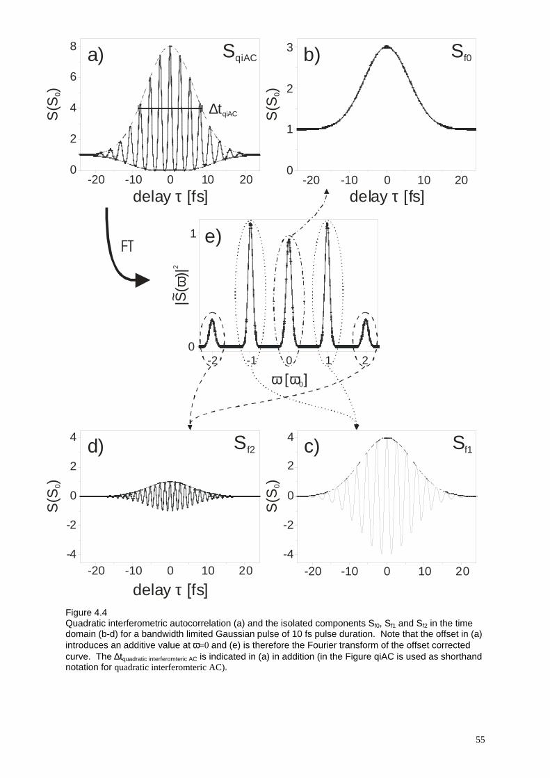
55
Figure 4.4 Quadratic interferometric autocorrelation (a) and the isolated components Sf0, Sf1 and Sf2 in the time domain (b-d) for a bandwidth limited Gaussian pulse of 10 fs pulse duration. Note that the offset in (a) introduces an additive value at ω=0 and (e) is therefore the Fourier transform of the offset corrected curve. The ∆tquadratic interferomteric AC is indicated in (a) in addition (in the Figure qiAC is used as shorthand notation for quadratic interferomteric AC).
0
1
ω ω [ ]0
0-1-2 1 2
|S(
)|ω
2~
-20 -10 0 10 200
1
2
3
delay [fs] τ
Sf0b)
delay [fs] τ
Sf1c)
delay [fs] τ
SqiACa)
Sf2d)
FT
-20 -10 0 10 200
2
4
6
8
-20 -10 0 10 20-4
-2
0
2
4
-20 -10 0 10 20-4
-2
0
2
4
S(S
) 0
S(S
) 0
S(S
) 0
S(S
) 0
∆tqiAC
e)
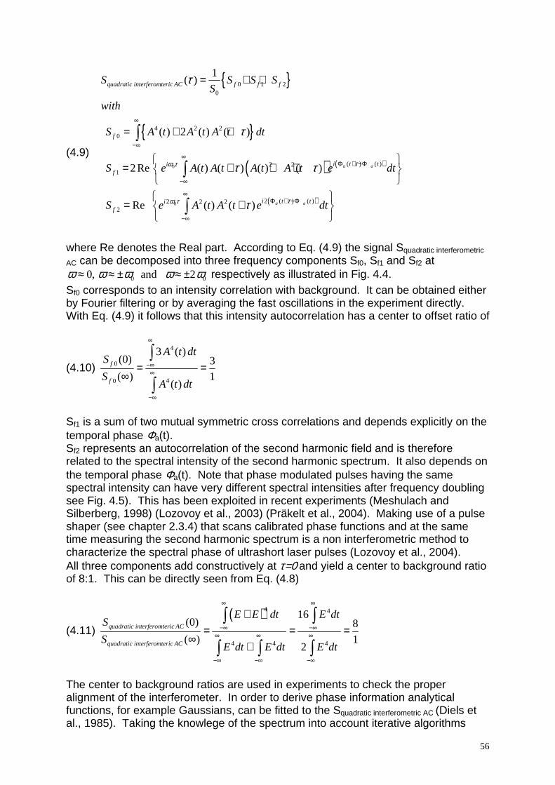
56
(4.9)
{ }
{ }
( ) ( )
( )
0
0
0 1 20
4 2 20
( ) ( )2 21
2 ( ) ( )2 2 22
1( )
( ) 2 ( ) ( )
2Re ( ) ( ) ( ) ( )
Re ( ) ( )
∞
−∞
∞Φ + −Φ
−∞
∞Φ + −Φ
−∞
= + +
= + +
= + + +
= +
∫
∫
∫
a a
a a
quadratic interferomteric AC f f f
f
i t tif
i t tif
S S S SS
with
S A t A t A t dt
S e A t A t A t A t e dt
S e A t A t e dt
τω τ
τω τ
τ
τ
τ τ
τ
where Re denotes the Real part. According to Eq. (4.9) the signal Squadratic interferometric
AC can be decomposed into three frequency components Sf0, Sf1 and Sf2 at
0 00, and 2ω ω ω ω ω≈ ≈ ± ≈ ± respectively as illustrated in Fig. 4.4. Sf0 corresponds to an intensity correlation with background. It can be obtained either by Fourier filtering or by averaging the fast oscillations in the experiment directly. With Eq. (4.9) it follows that this intensity autocorrelation has a center to offset ratio of
(4.10)
4
0
40
3 ( )(0) 3
( ) 1( )
∞
−∞∞
−∞
= =∞
∫
∫
f
f
A t dtS
SA t dt
Sf1 is a sum of two mutual symmetric cross correlations and depends explicitly on the temporal phase Φa(t). Sf2 represents an autocorrelation of the second harmonic field and is therefore related to the spectral intensity of the second harmonic spectrum. It also depends on the temporal phase Φa(t). Note that phase modulated pulses having the same spectral intensity can have very different spectral intensities after frequency doubling see Fig. 4.5). This has been exploited in recent experiments (Meshulach and Silberberg, 1998) (Lozovoy et al., 2003) (Präkelt et al., 2004). Making use of a pulse shaper (see chapter 2.3.4) that scans calibrated phase functions and at the same time measuring the second harmonic spectrum is a non interferometric method to characterize the spectral phase of ultrashort laser pulses (Lozovoy et al., 2004). All three components add constructively at τ=0 and yield a center to background ratio of 8:1. This can be directly seen from Eq. (4.8)
(4.11) ( )4 4
4 4 4
16(0) 8
( ) 12
quadratic interferomteric AC
quadratic interferomteric AC
E E dt E dtS
SE dt E dt E dt
∞ ∞
−∞ −∞∞ ∞ ∞
−∞ −∞ −∞
+= = =
∞+
∫ ∫
∫ ∫ ∫
The center to background ratios are used in experiments to check the proper alignment of the interferometer. In order to derive phase information analytical functions, for example Gaussians, can be fitted to the Squadratic interferometric AC (Diels et al., 1985). Taking the knowlege of the spectrum into account iterative algorithms
57
were reported that make no assumptions on the underlying pulse shapes (Peatross and Rundquist, 1998) (Naganuma et al., 1989). Both approaches deliver meaningful results only for linear chirp and in the case of nearly no noise. The influence of noise on autocorrelation measurements is discussed in (Van Stryland, 1979) (Diels and Rudolph, 1996). This is an important point as most often measurements are performed over an average of pulse trains. Other sources of systematic error in autocorrelation measurements are discussed in (Trebino, 2000). The ratio ∆tintAC/∆t is only valid for the intensity autocorrelation of a bandwidth limited pulse. For bandwidth limited Gaussian pulses the FWHM of a quadratic interferometric autocorrelation signal (taken at "4" in a 8:1 plot as displayed in Fig. 4.4a)) relates to the pulse duration by
(4.12) quadratic interferometric ACt1.6963
tforbandwidthlimited Gaussian pulses
∆=
∆
Fig. 4.5 compiles for different pulses the resulting interferometric autocorrelation traces together with the intensity autocorrelation and the spectrum at the second harmonic of the fundamental.

58
(a)Φ
a(t )
ω(t)
I (t)
1
3
5
7
τ [fs]
S(
)qu
adra
tic in
terfe
rom
etri
c AC
τ
1
3
5
7
S(
)in
t AC τ
PS
D (
)ω
ω [rad/fs]54 6
0,2
0,0
0,4
(b)Φ a(t)
ω(t)
I(t)
1
3
5
7
τ [fs]
S(
)qu
ad
ratic
inte
rfero
me
tric A
C
τ
1
3
5
7
S(
)in
t AC
τ
(c) Φa(t) ω(t)
I(t)
1
3
5
7
τ [fs]
S(
)q
uadr
atic
inte
rfero
me
tric
AC
τ
1
3
5
7
S(
)in
t AC
τ
(d)Φa(t)
ω(t)I(t)
1
3
5
7
τ [fs]
S(
)qu
adra
tic in
terfe
rom
etri
c A
C
τ
1
3
5
7
S(
)in
t ACτ
(e)Φa( t)
ω(t)
I (t)
1
3
5
7
τ [fs]
S(
)qu
adra
tic in
terfe
rom
etric
AC
τ
1
3
5
7
S(
)in
t AC
τ
PS
D (
)ω
ω [rad/fs]54 6
0,2
0,0
0,4
PS
D (
)ω
ω [rad/fs]54 6
0,2
0,0
0,4
PS
D (
)ω
ω [rad/fs]54 6
0,2
0,0
0,4
PS
D (
)ω
ω [rad/fs]54 6
0,2
0,0
0,4
-50 0 50 100-100
-50 0 50 100-100
-50 0 50 100-100
-50 0 50 100-100
-50 0 50 100-100

59
(f)Φa(t)
ω(t )
I(t )
1
3
5
7
τ [ fs]
S(
)qu
adra
tic in
terfe
rom
etric
AC
τ
1
3
5
7
S(
)int AC
τP
SD
()ω
ω [rad/fs]54 6
0,2
0,0
0,4
(g)
1
3
5
7
τ [fs]
S(
)qu
adr
atic
inte
rfero
met
ric A
C τ
1
3
5
7
S(
)int A
Cτ
(h)
1
3
5
7
τ [fs]
S(
)qu
adra
tic in
terfe
rom
etric
AC
τ
1
3
5
7
S(
)int A
Cτ
(i)
1
3
5
7
τ [fs]
S(
)qu
adra
tic in
terfe
rom
etric
AC
τ
1
3
5
7
S(
)int A
Cτ
(j)Φ a(t)
ω(t)
I(t)
1
3
5
7
τ [fs]
S(
)qu
adra
tic in
terfe
rom
etric
AC
τ
1
3
5
7
S(
)int A
Cτ
PS
D (
)ωω [rad/fs]
54 6
0,2
0,0
0,4
PS
D (
)ω
ω [rad/fs]54 6
0,2
0,0
0,4
PS
D (
)ω
ω [rad/fs]54 6
0,2
0,0
0,4
PS
D (
)ω
ω [rad/fs]54 6
0,2
0,0
0,4
Φa(t)
ω(t)
I (t)
Φa(t )
ω(t )I(t)
Φ a(t)
ω(t)
I(t)
-50 0 50 100-100
-50 0 50 100-100
-50 0 50 100-100
-50 0 50 100-100
-50 0 50 100-100
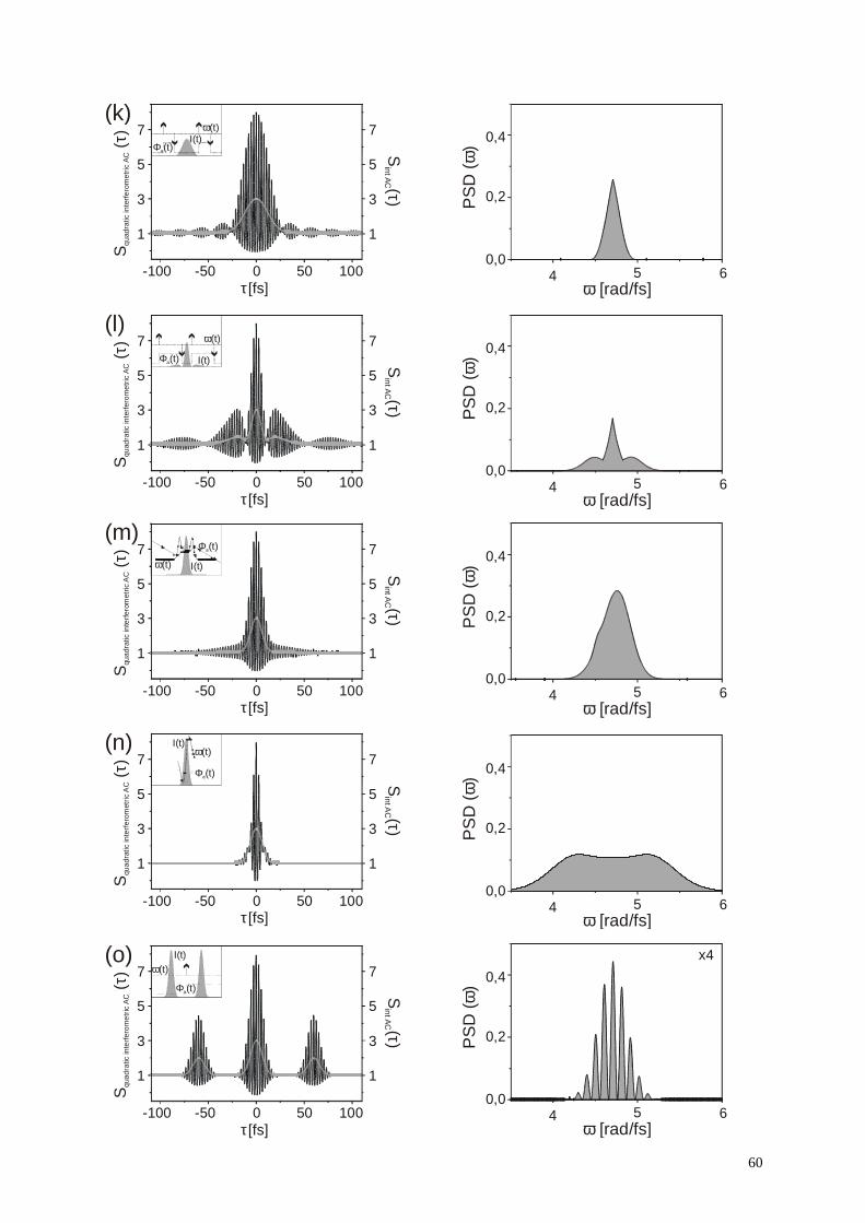
60
(k)
1
3
5
7
τ [fs]
S(
)qu
adra
tic in
terf
erom
etric
AC
τ
1
3
5
7
S(
)int A
Cτ
PS
D (
)ω
ω [rad/fs]54 6
0,2
0,0
0,4
(l)
1
3
5
7
τ [fs]
S(
)qu
adra
tic in
terf
erom
etric
AC
τ
1
3
5
7
S(
)int A
Cτ
(m)
1
3
5
7
τ [fs]
S(
)qu
adra
tic in
terf
erom
etric
AC
τ
1
3
5
7
S(
)int A
Cτ
(n)
1
3
5
7
τ [fs]
S(
)qu
adra
tic in
terf
erom
etric
AC
τ
1
3
5
7
S(
)int A
Cτ
(o)
1
3
5
7
τ [fs]
S(
)qu
adra
tic in
terf
erom
etric
AC
τ
1
3
5
7
S(
)int A
Cτ
PS
D (
)ω
ω [rad/fs]54 6
0,2
0,0
0,4
PS
D (
)ω
ω [rad/fs]54 6
0,2
0,0
0,4
PS
D (
)ω
ω [rad/fs]54 6
0,2
0,0
0,4
PS
D (
)ω
ω [rad/fs]54 6
0,2
0,0
0,4
Φa(t)
ω(t)
I(t)
Φa(t)
ω(t)I(t)
Φa(t)
ω(t)I(t)
Φa(t)
ω(t) I(t)
-50 0 50 100-100
-50 0 50 100-100
-50 0 50 100-100
-50 0 50 100-100
-50 0 50 100-100
Φa(t)
ω(t)I(t) x4
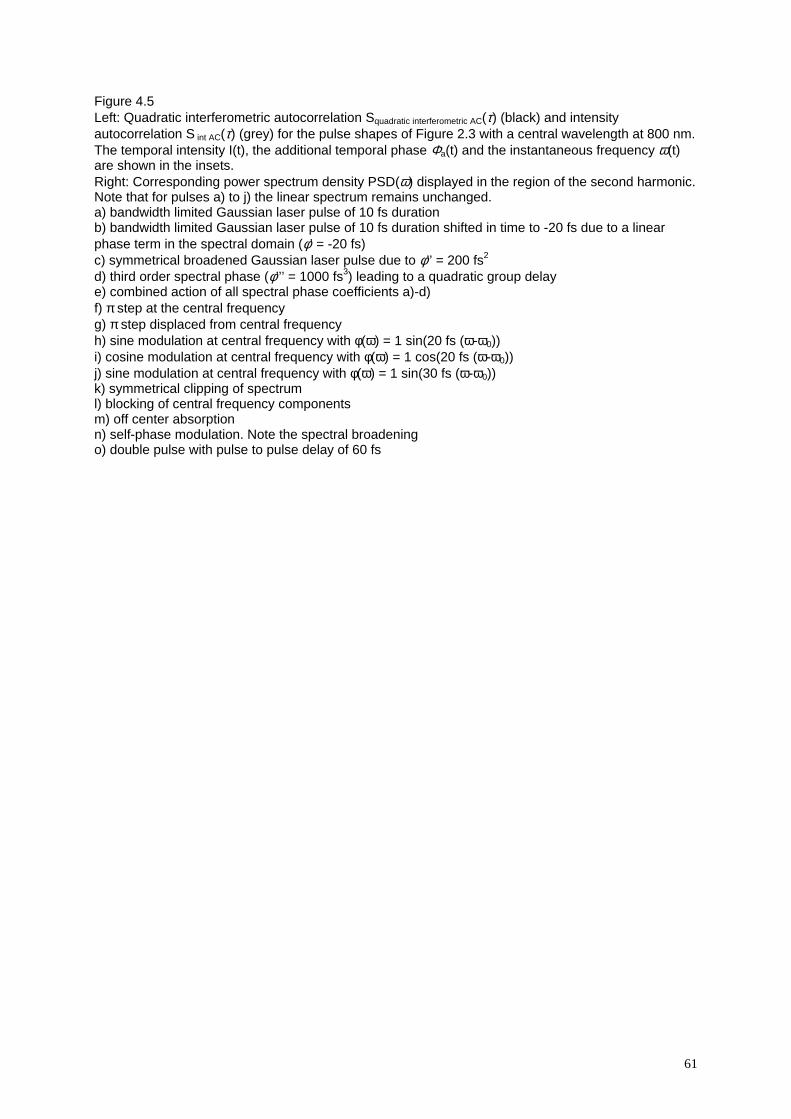
61
Figure 4.5 Left: Quadratic interferometric autocorrelation Squadratic interferometric AC(τ) (black) and intensity autocorrelation S int AC(τ) (grey) for the pulse shapes of Figure 2.3 with a central wavelength at 800 nm. The temporal intensity I(t), the additional temporal phase Φa(t) and the instantaneous frequency ω(t) are shown in the insets. Right: Corresponding power spectrum density PSD(ω) displayed in the region of the second harmonic. Note that for pulses a) to j) the linear spectrum remains unchanged. a) bandwidth limited Gaussian laser pulse of 10 fs duration b) bandwidth limited Gaussian laser pulse of 10 fs duration shifted in time to -20 fs due to a linear phase term in the spectral domain (φ’ = -20 fs) c) symmetrical broadened Gaussian laser pulse due to φ’’ = 200 fs2 d) third order spectral phase (φ’’’ = 1000 fs3) leading to a quadratic group delay e) combined action of all spectral phase coefficients a)-d) f) π step at the central frequency g) π step displaced from central frequency h) sine modulation at central frequency with φ(ω) = 1 sin(20 fs (ω-ω0)) i) cosine modulation at central frequency with φ(ω) = 1 cos(20 fs (ω-ω0)) j) sine modulation at central frequency with φ(ω) = 1 sin(30 fs (ω-ω0)) k) symmetrical clipping of spectrum l) blocking of central frequency components m) off center absorption n) self-phase modulation. Note the spectral broadening o) double pulse with pulse to pulse delay of 60 fs

62
4.4 Time frequency methods As described above, the interferometric autocorrelation even together with the independently measured spectrum give not sufficient information to characterize arbitrary shaped ultrashort laser pulses with respect to their temporal amplitude A(t) or temporal intensity I(t) and the temporal phase function Φa(t) or their frequency domain counterparts (see chapter 2.2). Techniques have emerged that operate not in the time or frequency domain but in the "joint time-frequency" domain involving both temporal resolution and frequency resolution simultaneously (Cohen, 1989) (Quian and Chen, 1996) and being able to completely determine the pulse shape (Trebino, 2000). For illustration purposes we start with an example from music: in order to describe a line of music we use notes. The frequency is indicated by the pitch of the note and the duration of the note indicates how long the frequency has to be held. The sheet of music will tell us in what order the notes have to be played and additional information like "piano" and "forte" is given to indicate the intensity to be played. The first few notes of Beethoven's 5th symphony are given as an example in Fig. 4.6a. If an orchestra is playing the music and we wish to graphically record the music, a spectrogram Spectrogram(ω,τ) is a useful quantity. A spectrogram of a function f(t) is defined as the energy density spectrum of a short-time Fourier Transform STFT(ω,τ)
(4.13) 2
2( , ) ( , ) ( ) ( ) i t
pectrogramS STFT f t g t e dtωω τ ω τ τ∞
−
−∞
≡ = −∫
where g(t-τ) denotes the gate (or window) function. The concept behind it is simple and powerful. If we want to analyze what is happening at a particular time, we just use a small portion of the signal centered at that time, calculate its spectrum and do it for each instant of time. A spectrogram corresponding to the beginning of Beethoven's 5th symphony is shown in Fig. 4.6b. Fig. 4.7 shows the concept of STFT on a complicated electric field of a laser. Once an electric field is retrieved in amplitude and phase there are other time - frequency distributions in use for displaying the data like for example the Wigner (Cohen, 1989) (Scully and Zubairy, 1995) (Schleich, 2001) (Bartelt et al., 1980) (Paye and Migus, 1995) and
63
Figure 4.6 Sheet of music (a) and corresponding spectrogram (b) of Beethoven's 5th symphony Husimi representations (Lee, 1994) (Lalovic et al., 1992). A quantity closely related to the spectrogram is the sonogram Sonogram(ω,τ)
(4.14) 2
'( , ) ( ') ( ') 'ionogramS f g e dω τω τ ω ω ω ω
∞+
−∞
≡ −∫ � �
where ( ')g ω ω−� is a frequency gate in analogy to the time gate ( )g t τ− used in the spectrogram. If ( )g ω� is the Fourier transform of g(t) then it can be shown that the sonogram is equivalent to the spectrogram (Trebino, 2000). In ultrafast optics the gate to record the spectrogram or the sonogram is usually the pulse itself.
time [s]
aud
io fr
equ
ency
Ludwig van Beethoven Symphony No. 5C minor op. 67Allegro con brio
a)
b)
0 0.5 1.0 1.5 2.0 2.5

64
Figure 4.7 Illustration of a short time Fourier-Transform on behalf of a complicated electric field. a) Electric field as a function of time b) Power spectrum density as a function of frequency c) Gating the electric field; four different time delays are shown d) Power spectrum density for each gate e) Spectrogram, revealing an oscillating instantaneous frequency as a function of time beeing the origine for the complicated electric field in a)
τ3τ2 τ4τ1
τ3τ2 τ4τ1
frequency
win
dow
ed
PS
Del
ectr
ic fi
eld
PS
Del
ectr
ic fi
eld
time t
time τ
time t
fre
quen
cy
time τ
g(t- )τc)
b)
d)
f)
a)

65
4.4.1 Spectrogram based methods Recording a spectrogram is accomplished experimentally by gating the pulse with a variable delayed replica of the pulse in an instantaneous nonlinear optical medium followed by spectrally resolving the gated pulse. The basic optical layout of such a device is almost the same as a non collinear autocorrelation setup depicted in Fig. 4.2b). Only the detector has to be replaced by a spectrometer and camera system in order to spectrally resolve the gated pulse. The corresponding technique has been termed Frequency-Resolved Optical Gating (FROG) and is described in great detail in (Trebino et al., 1997) (Trebino, 2000) and references therein. Depending on the instantaneous nonlinear optical effect used to gate the pulse in FROG, several different FROG geometries have been investigated (the set up of Fig. 4.2b) would correspond to a SHG FROG). These geometries can also be implemented as single shot devices, similar to the single shot autocorrelator depicted in Fig. 4.3. The FROG trace IFROG(ω,τ), that is a plot of frequency (wavelength) versus delay, is a spectrogram of the complex amplitude Ec (see (2.15)) (Trebino, 2000). Neglecting any prefactors, different nonlinear optical effects yield the following expressions according to (Trebino et al., 1997) (Trebino, 2000): Polarization-Gate (PG) FROG:
(4.15) 2
2( , ) ( ) ( )PG i t
FROG c cI E t E t e dtωω τ τ∞
−
−∞
= −∫
In a crossed polarizers arrangement for the probe pulse this technique makes use of induced birefringence in fused silica in the presence of the gate pulse. The third order optical nonlinearity is the electronic Kerr effect. The FROG traces obtained by this method are very intuitive (see Fig. 4.8) Self-Diffraction (SD) FROG
(4.16)
2
*2( , ) ( ) ( )SD i tFROG c cI E t E t e dtωω τ τ
∞−
−∞
= −∫
In this approach the two beams (same polarization) generate a sinusoidal intensity pattern in the nonlinear medium (for example fused silica) and hence introduce a material grating, which diffracts each beam. One of the diffracted beams is then the signal beam sent to the spectrometer. Transient-Grating (TG) FROG
(4.17) 2
*1 2 3( , ) ( ) ( ) ( )TG i t
FROG c c cI E t E t E t e dtωω τ τ∞
−
−∞
= −∫
This is a three beam set up, where two pulses are overlapped in time and space at the optical - Kerr medium (for example fused silica) producing a refractive index grating similar as in SD FROG. In TG a third pulse is variably delayed and overlapped in the fused silica and is diffracted by the induced grating producing the
66
signal beam for the spectrometer. The beams in TG geometry (three input and one output) are kept nearly collinear and form a so called BOXCARS arrangement, where the four spots appear in the corners of a rectangle when placing a card into the beams after the nonlinear medium. As TG is a phase-matched process, the sensitivity is higher compared to the SD approach. Depending on which pulse is variably delayed – with the other two coincident in time – the TG FROG trace is mathematically equivalent to the PG FROG (pulse one or three is delayed) or to the SD FROG (pulse two is delayed). Third-Harmonic-Generation (THG) FROG
(4.18) 2
2( , ) ( ) ( )THG i tFROG c cI E t E t e dtωω τ τ
∞−
−∞
= −∫
This method makes use of third harmonic generation as the nonlinear process. Second-Harmonic-Generation (SHG) FROG
(4.19) 2
( , ) ( ) ( )SHG i tFROG c cI E t E t e dtωω τ τ
∞−
−∞
= −∫
SHG FROG involves spectrally resolving a standard SHG-based noncollinear intensity autocorrelator, which yields always symmetric traces resulting in a direction of time ambiguity for the SHG FROG. This ambiguity can experimentally be removed for example by placing a piece of glass in the beam before the beam splitter in order to introduce positive chirp or in order to create satellite pulses via surface reflections. Because of its high sensitivity and as it is based on a standard SHG autocorrelator, this method is widely employed. Examples of SHG FROG traces for various pulse shapes are given in Fig. 4.8. A comparison of the different approaches is given in Table 4.1. Various calculated traces for common ultrashort pulse distortions for the PG and the SHG FROG geometries are given in Fig. 4.8. Calculated FROG traces for the other beam geometries are given in (Trebino et al., 1997). Measured FROG traces for different geometries are compiled in (Trebino, 2000). It is important to note, that knowledge of the spectrogram (or sonogram) of the electric field of an ultrashort laser pulse is sufficient to completely determine the electric field in amplitude and phase (besides some ambiguities such as the absolute phase) because a spectrogram is equivalent to the two dimensional phase retrieval problem in image science and astronomy (Stark, 1987). In general, phase retrieval is the problem of finding a function knowing only the magnitude (but not the phase) of its Fourier transform. Phase retrieval for a function of one variable is impossible. For example, knowledge of a pulse spectrum does not fully determine the pulse as infinitely many different pulses have the same spectrum (see for example Fig. 2.3 a)-j)). But phase retrieval for a function of two variables is possible and the FROG trace can be rewritten as the squared magnitude of a two dimensional Fourier transform (Trebino et al., 1997). There exist very sophisticated iterative retrieval procedures, which can rapidly retrieve the pulse from the FROG trace with update rates up to several Hz (Kane, 1999).

67
Geometry PG SD TG THG SHG
Nonlinearity
χ(3)
χ(3)
χ(3)
χ(3)
χ(2)
Sensitivity (single shot)
~ 1 µJ
~ 10 µJ
~ 0.1 µJ
~0.03 µJ
~ 0.01 µJ
Sensitivity (multi shot)
~ 100 nJ
~ 1000 nJ
~ 10 nJ
~ 3nJ
~ 0.001 nJ
Advantages
Intuitive traces; Automatic phase
matching
Intuitive traces; Deep UV capability;
Background - free; Sensitive;
Intuitive traces; Deep UV capability
Sensitive; Very large bandwidth
Very sensitive
Disadvantages
Requires polarizers Requires thin medium; Not phase matched
Three beams Unintuitive traces; Very short λ signal
Unintuitive traces; Short λ signal
Ambiguities
None known
None known
None known
Relative phase of multiple pulses
φ, φ +/- 2π/3
Relative phase of multiple pulses
φ, φ + π; Direction of time
Schematics
ω ω
ωω χ(3)
D
ω ω
ωω
χ(3)
D
ω
3ωω χ(3)
D
ω
2ω
ω χ(2)
D
WP
P
Pω
ωχ(3)
D

68
Table 4.1 Comparison of different FROG geometries (PG = polarization gate; SD = self diffraction; TG = transient grating; THG = third harmonic generation; SHG = second harmonic generation). Sensitivities are only approximated and assume 800 nm 100 fs pulses focused to about 100 µm (10 µm for THG) to be measured. In the schematics only the part involving the non linear optical effect characterized by its non linearity is displayed. Not shown are delay lines and various lenses as they are common to all set ups and similar to the optical layouts shown in figure 4.2b) and figure 4.3. Solid lines indicate input pulses and dashed lines indicate signal pulses. The frequencies shown (ω, 2ω, 3ω) are the carrier frequencies of the pulses taking part and indicate whether the signal pulse has the same carrier frequency as the input pulse or is shifted as in SHG and THG. D denotes a detector being composed of a spectrometer and camera system. (WP = wave plate; P = polarizer) (after (Trebino, 2000)) In the following some additional attributes of FROG techniques are summarized, that partially also hold for sonogram methods:
• As the FROG trace consists of NxN points, the intensity and phase on the other side only have 2N points the FROG trace overdetermines the pulse. This gives rise to an increased robustness of the two-dimensional methods and to an improved immunity towards measurement noise. The nonconvergence of the FROG algorithm therefore can be a hint to the presence of systematic errors.
• Other than autocorrelation techniques, FROG offers a built in consistency check to detect systematic errors. It involves computing the “marginals” of the FROG trace, that is, integrals of the trace with respect to delay or frequency. The marginals can be compared to the independently measured spectrum or autocorrelation. For an SHG FROG the time marginal yields the intensity autocorrelation and the frequency marginal yields the second harmonic spectrum. The marginals of the SHG FROG traces in Fig. 4.8 are therefore given in the corresponding pictures of Fig. 4.5.
• FROG can also be used in a cross-correlation variant named XFROG (Linden et al., 1999). In this case a known pulse is used to gate an unknown pulse (usually derived from the known one), where no spectral overlap between the pulses is required. Via sum frequency generation or difference frequency generation or other nonlinear processes, pulses in the UV and IR spectral range can be characterized. The technique has been refined for measuring pulses in the Attojoule (per pulse) regime and is capable to measure pulses with poor spatial coherence and random phase, such as fluorescence (Zhang et al., 2003).
• In the sub 10 fs range SHG FROG has been demonstrated down to 4.5 fs pulse duration with the help of Type I phase matching in a 10 µm thick BBO crystal (Baltuska et al., 1998). In this regime the noncollinear beam geometry can also introduce beam smearing arte facts. Type II phase matching allows the use of a collinear SHG FROG geometry, which is free of geometrical smearing (Fittinghoff et al., 1998) (Gallmann et al., 2000a). The FROG traces generated in this arrangement don't contain optical fringes associated with interferometric autocorrelations and, therefore, can be processed by existing SHG FROG algorithms.
• Making use of a thick SHG crystal as a frequency filter (O'Shea et al., 2001) (Radzewicz et al., 2000) allows for the construction of an extrem simple and robust FROG set up demonstrated for 800 nm pulses in the range from 20 fs
69
to 5 ps for different spectral widths of the ultrashort pulses. The device was termed GRENOUILLE (Grating-Eliminated No-nonsense Observation of Ultrafast Incident Laser Light E-fields) (Trebino, 2000). Spatial temporal distortions like spatial chirp and pulse front tilt can be measured via GRENOUILLE as well (Akturk et al., 2003a) (Akturk et al., 2003b) (spatial chirp: each frequency is displaced in the transverse spatial coordinates resulting often from misaligned prism pairs and tilted windows; pulse front tilt: the pulse group fronts (intensity contours) are tilted with respect to the perpendicular to the propagation direction resulting from residual angular dispersion after pulse compressor or stretcher units).
• The wavelength limitation due to nonlinear optical processes can be circumvented by the use of multi-photon ionization as nonlinearity. Measurements of interferometrically recorded energy resolved photoelectron spectra generated by above-threshold ionization were demonstrated to yield FROG-type time-frequency distributions which were used to characterize ultrashort laser pulses (Winter et al., 2006). This approach is potentially applicable to the XUV wavelength region.
Figure 4.8 Calculated FROG traces for various ultrashort pulse shapes with a central wavelength at 800 nm according to the pulses displayed in figure 2.3. Left: Polarization gate (PG) FROG Right: Second harmonic generation (SHG) FROG The temporal intensity I(t), the additional temporal phase Φa(t) and the instantaneous frequency ω(t) are shown in the insets as a reminder. a) bandwidth limited Gaussian laser pulse of 10 fs duration b) bandwidth limited Gaussian laser pulse of 10 fs duration shifted in time to -20 fs due to a linear phase term in the spectral domain (φ’ = -20 fs) c) symmetrical broadened Gaussian laser pulse due to φ’’ = 200 fs2 d) third order spectral phase (φ’’’ = 1000 fs3) leading to a quadratic group delay e) combined action of all spectral phase coefficients a)-d) f) π step at the central frequency g) π step displaced from central frequency h) sine modulation at central frequency with φ(ω) = 1 sin(20 fs (ω-ω0)) i) cosine modulation at central frequency with φ(ω) = 1 cos(20 fs (ω-ω0)) j) sine modulation at central frequency with φ(ω) = 1 sin(30 fs (ω-ω0)) k) symmetrical clipping of spectrum l) blocking of central frequency components m) off center absorption n) self-phase modulation. Note the spectral broadening o) double pulse with pulse to pulse delay of 60 fs

70
(a)
(b)
(c)
(d)
(e)
Φa(t )
ω(t)I(t )
Φa(t)
ω (t)
I(t)
Φa(t)
ω(t)
I(t)
Φa(t )
ω (t)
I(t)
Φa( t) ω(t)
I(t)
ω [r
ad/fs
]
5,0
4,0
6,0
-75 750τ [fs]
ω [r
ad/fs
]
5,0
4,0
6,0
-75 750
τ [fs]ω
[rad
/fs]
5,0
4,0
6,0
-75 750τ [fs]
ω [r
ad/fs
]
5,0
4,0
6,0
-75 750τ [fs]
ω [r
ad/fs
]
5,0
4,0
6,0
-75 750
τ [fs]
2,0
-75
3,0
750τ [fs]
ω [r
ad/fs
]
2,0
-75
3,0
750
τ [fs]
ω [r
ad/
fs]
2,0
-75
3,0
750
τ [fs]
ω [r
ad/
fs]
2,0
-75
3,0
750
τ [fs]
ω [r
ad/
fs]
2,0
-75
3,0
750
τ [fs]
ω [r
ad/fs
]

71
(f)
(g)
(h)
(i)
(j)
Φa( t)
ω(t)
I(t)
2,0
-75
3,0
750
τ [fs]
ω [r
ad/fs
]Φa(t )
ω(t)
I(t)
Φa(t)
ω (t)I(t )
Φa(t)
ω(t)
I(t)
Φa(t)ω (t)
I(t)
ω [r
ad/fs
]
5,0
4,0
6,0
-75 750
τ [fs]
ω [r
ad/fs
]
5,0
4,0
6,0
-75 750
τ [fs]ω
[rad
/fs]
5,0
4,0
6,0
-75 750
τ [fs]
ω [r
ad/fs
]
5,0
4,0
6,0
-75 750
τ [fs]
ω [r
ad/f
s]
5,0
4,0
6,0
-75 750τ [fs]
2,0
-75
3,0
750
τ [fs]
ω [r
ad/fs
]
2,0
-75
3,0
750
τ [fs]
ω [r
ad/fs
]
2,0
-75
3,0
750
τ [fs]
ω [r
ad/fs
]
2,0
-75
3,0
750τ [fs]
ω [r
ad/f
s]

72
(k)
(l)
(m)
(n)
(o)
Φa(t)
ω(t)I(t)
Φa(t)
ω(t)
I(t)
Φa(t)
ω(t) I(t)
ω [r
ad/fs
]
5,0
4,0
6,0
-75 750
τ [fs]
ω [r
ad/fs
]
5,0
4,0
6,0
-75 750
τ [fs]ω
[rad
/fs]
5,0
4,0
6,0
-75 750
τ [fs]
ω [r
ad/fs
]
5,0
4,0
6,0
-75 750
τ [fs]
ω [r
ad/fs
]
5,0
4,0
6,0
-75 750
τ [fs]
2,0
-75
3,0
750
τ [fs]
ω [r
ad/fs
]
2,0
-75
3,0
750
τ [fs]
ω [r
ad/fs
]
2,0
-75
3,0
750
τ [fs]
ω [r
ad/fs
]
2,0
-75
3,0
750
τ [fs]
ω [r
ad/fs
]
2,0
-75
3,0
750
τ [fs]
ω [r
ad/fs
] Φa(t)
ω(t)I(t)
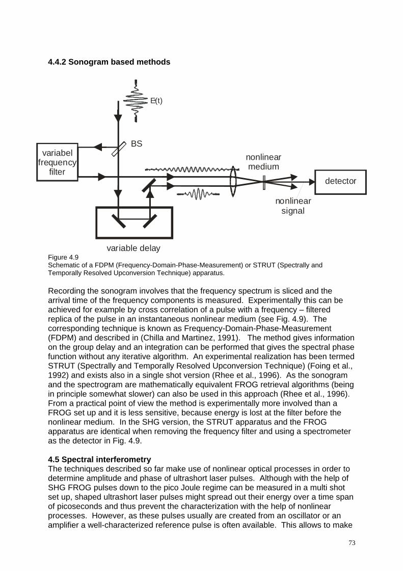
73
4.4.2 Sonogram based methods
Figure 4.9 Schematic of a FDPM (Frequency-Domain-Phase-Measurement) or STRUT (Spectrally and Temporally Resolved Upconversion Technique) apparatus. Recording the sonogram involves that the frequency spectrum is sliced and the arrival time of the frequency components is measured. Experimentally this can be achieved for example by cross correlation of a pulse with a frequency – filtered replica of the pulse in an instantaneous nonlinear medium (see Fig. 4.9). The corresponding technique is known as Frequency-Domain-Phase-Measurement (FDPM) and described in (Chilla and Martinez, 1991). The method gives information on the group delay and an integration can be performed that gives the spectral phase function without any iterative algorithm. An experimental realization has been termed STRUT (Spectrally and Temporally Resolved Upconversion Technique) (Foing et al., 1992) and exists also in a single shot version (Rhee et al., 1996). As the sonogram and the spectrogram are mathematically equivalent FROG retrieval algorithms (being in principle somewhat slower) can also be used in this approach (Rhee et al., 1996). From a practical point of view the method is experimentally more involved than a FROG set up and it is less sensitive, because energy is lost at the filter before the nonlinear medium. In the SHG version, the STRUT apparatus and the FROG apparatus are identical when removing the frequency filter and using a spectrometer as the detector in Fig. 4.9. 4.5 Spectral interferometry The techniques described so far make use of nonlinear optical processes in order to determine amplitude and phase of ultrashort laser pulses. Although with the help of SHG FROG pulses down to the pico Joule regime can be measured in a multi shot set up, shaped ultrashort laser pulses might spread out their energy over a time span of picoseconds and thus prevent the characterization with the help of nonlinear processes. However, as these pulses usually are created from an oscillator or an amplifier a well-characterized reference pulse is often available. This allows to make
E(t)
BS
variable delay
nonlinearmedium
nonlinearsignal
variabelfrequency
filterdetector

74
Figure 4.10 Basic set-up for Spectral Interferometry (SI) in order to characterize the phase difference between an ultrashort (signal) pulse E(t) and a time delayed reference pulse E(t)ref. use of highly sensitive linear techniques to determine amplitude and phase of an ultrashort laser pulse. The technique is named Spectral Interferometry (SI) or also frequency-domain interferometry or Fourier-Transform spectral interferometry (Froehly et al., 1973;Piasecki et al., 1980;Reynaud et al., 1989;Lepetit et al., 1995;Trebino, 2000). The basic SI set up is depicted in Fig. 4.10. A well characterized reference pulse Eref(t) and a modified signal pulse E(t) derived from an experiment or a pulse shaper are directed collinearly into a spectrometer. The measured SI spectrum SSI(ω) is proportional to the square of the Fouriertransform of the sum of the two fields:
(4.20)
{ }
( )
2
2
2( ) ( )
( ) ( )
( ) ( ) ( )
( ) ( )
( ) ( )
( ) ( ) ( ) ( ) . .
( ) ( ) 2 ( ) ( ) cos( ( ) ( ) )
ref
ref
SI ref
iref
i i iref
i i iref ref
ref ref ref
S Fouriertransform E t E t
E E e
I e I e
I I I I e c c
I I I I
ωτ
φ ω φ ω ωτ
φ ω φ ω ωτ
ω τ
ω ω
ω ω
ω ω ω ω
ω ω ω ω φ ω φ ω ωτ
−
− − −
− −
∝ + −
∝ +
∝ +
= + + +
= + + − −
� �
The phase difference (4.21) ( ) ( ) ( )refφ ω φ ω φ ω∆ = −
can be extracted from the measured SSI(ω). Using the arcosine function is not recommended because experimental noise can lead to large phase errors (Lepetit et al., 1995). Commonly a Fourier Transform technique is used (Takeda et al., 1981) (Lepetit et al., 1995) where the phase difference is extracted by the Fourier transform of the measured spectrum, ignoring the negative and zero frequency components and shifting the positive frequency components to dc in order to remove the delay term ie ωτ− . An inverse Fourier transform then yields the phase difference ( )∆φ ω . With the help of the known reference phase ( )refφ ω finally ( )φ ω is obtained.
Reference In
Signal InE(t) E (t)ref
Spectrometerτ

75
Figure 4.11 Experimental set up for real-time Spatial-Spectral Interference (SSI) measurements. (after (Meshulach et al., 1997)). In the following some attributes of SI are summarized:
• SI requires the spectrum of the reference pulse to contain completely the spectrum of the unknown pulse.
• If the reference pulse and the signal pulse are identical, the phase difference is zero. The remaining oscillations on the spectrum due to the delay term are a convenient tool to adjust for example interferometric autocorrelator set ups.
• Using for characterization of the reference pulse the FROG technique, the combined technique was termed TADPOLE (Temporal Analysis by Dispersing a Pair Of Light E-fields) (Fittinghoff et al., 1996) (Trebino, 2000).
• SI is a heterodyne technique and amplifies the generally weak signal pulse (see Eq. (4.20)). With the help of TADPOLE, pulse trains with an energy per pulse in the zeptojoule (zepto = 10-21) regime have been analyzed (Fittinghoff et al., 1996).
• Once the reference phase is known, the phase retrieval does not require an iterative procedure and is therefore fast. This allows for example for synthesis of arbitrary laser pulse shapes with the help of feedback-controlled femtosecond pulse shaping techniques (Brixner et al., 2000). Together with the high sensitivity, TADPOLE is well suited to characterize complex shaped femtosecond laser pulses. Furthermore, in a dual channel set up SI has been used to characterize complex polarization shaped femtosecond laser pulses (Brixner et al., 2002). The set up to characterize time dependent polarization profiles has been called POLLIWOG (POLarization-Labeled Interference versus Wavelength for Only a Glint) (Walecki et al., 1997).
• SI can also be implemented in a spatial variation, where the reference pulse and the signal pulse propagate at an angle of 2 Θ with respect to each other (see Fig. 4.11). The frequency components of the optical fields of the two propagating pulses are mapped in one dimension by a diffraction grating and a cylindrical lens and interfere at the focal plane of the lens. The technique is named Spatial-Spectral Interference (SSI). The corresponding device is a convenient tool for optimizing various set ups such as pulse shapers and compressors as the fringe patterns are displayed in real time and the information is encoded in an intuitively interpretable pattern (Meshulach et al., 1997). A comparison of calculated SI and SSI traces for various ultrashort pulse distortions is given in Fig. 4.12.
grating cylindrical lens
reference
signal
detector
f
76
• There also exists a self-referencing variant of SI which does not require separate characterization of the reference pulse. This technique is called SPIDER(Spectral Phase Interferometry for Direct Electric Field Reconstruction) (Iaconis and Walmsley, 1998) (Iaconis and Walmsley, 1999). It involves appropriate temporal stretching of a reference pulse followed by sum-frequency generation with two well displaced copies of the unstretched input pulse. This technique was succesfully demonstrated for characterization of ultrashort pulses in the few cycle regime (Gallmann et al., 1999). Due to the nonlinear process involved, SPIDER is less sensitive in comparison to TADPOLE. A comparison of SHG-FROG and SPIDER for sub ten femtosecond pulse characterization is given in (Gallmann et al., 2000b). A spatially resolved version of SPIDER was also demonstrated (Gallmann et al., 2001). A set up that is capable to characterize a pulse at the interaction point of an experiment was named Zero Additional Phase (ZAP) SPIDER and demonstrated for visible and sub 20 femtosecond ultraviolet pulses (Baum et al., 2004).
Figure 4.12 Calculated SI (Spectral Interference) and SSI (Spatial Spectral Interference) traces for various ultrashort pulse shapes with a central wavelength at 800 nm according to the pulses displayed in figure 2.3. Left: SI: the time delay between both pulses is 100 fs. Right: SSI the angle 2Θ between both beams is 2°. The temporal intensity I(t), the additional temporal phase Φa(t) and the instantaneous frequency ω(t) are shown in the insets as a reminder. a) bandwidth limited Gaussian laser pulse of 10 fs duration b) bandwidth limited Gaussian laser pulse of 10 fs duration shifted in time to -20 fs due to a linear phase term in the spectral domain (φ’ = -20 fs) c) symmetrical broadened Gaussian laser pulse due to φ’’ = 200 fs2 d) third order spectral phase (φ’’’ = 1000 fs3) leading to a quadratic group delay e) combined action of all spectral phase coefficients a)-d) f) π step at the central frequency g) π step displaced from central frequency h) sine modulation at central frequency with φ(ω) = 1 sin(20 fs (ω-ω0)) i) cosine modulation at central frequency with φ(ω) = 1 cos(20 fs (ω-ω0)) j) sine modulation at central frequency with φ(ω) = 1 sin(30 fs (ω-ω0)) k) symmetrical clipping of spectrum l) blocking of central frequency components m) off center absorption n) self-phase modulation. Note the spectral broadening o) double pulse with pulse to pulse delay of 60 fs

77
(a)Φa(t)
ω(t)
I(t)
ω [rad/fs]2,42,0 2,8
(b)Φa(t )
ω(t)
I(t)
(c) Φa(t) ω (t)
I(t)
(d)Φ a(t)
ω(t)I (t)
(e)Φa(t)
ω(t)
I(t)
0
50
100
150
ω [rad/fs]
200
250
1,5 2,0 2,5 3,0
50
100
150
ω [rad/fs]
200
250
1,5 2,0 2,5 3,0
50
100
150
ω [rad/fs]
200
250
1,5 2,0 2,5 3,0
50
100
150
ω [rad/fs]
200
250
1,5 2,0 2,5 3,0
50
100
150
ω [rad/fs]
200
250
1,5 2,0 2,5 3,0
0
0
0
0
ω [rad/fs]2,42,0 2,8
ω [rad/fs]2,42,0 2,8
ω [rad/fs]2,42,0 2,8
ω [rad/fs]2,42,0 2,8
I()
ωI(
)ω
I()ω
I()
ωI(
)ω
x (ω
)
0
x (ω
)
0
x (ω
)
0
x (ω
)
0
x (ω
)
0

78
(f)
(g)
(h)
(i)
(j)
0
50
100
150
ω [rad/fs]
200
250
1,5 2,0 2,5 3,0
50
100
150
ω [rad/fs]
200
250
1,5 2,0 2,5 3,0
50
100
150
ω [rad/fs]
200
250
1,5 2,0 2,5 3,0
50
100
150
ω [rad/fs]
200
250
1,5 2,0 2,5 3,0
50
100
150
ω [rad/fs]
200
250
1,5 2,0 2,5 3,0
0
0
0
0
Φa(t )
ω(t)
I(t)
Φa(t)ω(t)
I (t)
Φa(t)
ω(t)I(t)
Φ a(t)
ω(t)
I(t)
Φa(t)ω(t)
I (t)
ω [rad/fs]2,42,0 2,8
ω [rad/fs]2,42,0 2,8
ω [rad/fs]2,42,0 2,8
ω [rad/fs]2,42,0 2,8
ω [rad/fs]2,42,0 2,8
x (ω
)
0
x (ω
)
0
x (ω
)
0
x (ω
)
0
x (ω
)
0
I()ω
I()
ωI(
)ω
I()ω
I()
ω

79
(k)
(l)
(m)
(n)
(o)
0
50
100
150
ω [rad/fs]
200
250
1,5 2,0 2,5 3,0
50
100
150
ω [rad/fs]
200
250
1,5 2,0 2,5 3,0
50
100
150
ω [rad/fs]
200
250
1,5 2,0 2,5 3,0
50
100
150
ω [rad/fs]
200
250
1,5 2,0 2,5 3,0
50
100
150
ω [rad/fs]
200
250
1,5 2,0 2,5 3,0
0
0
0
0
Φa(t)
ω(t)I(t)
Φa(t)
ω(t)
I(t)
Φa(t)
ω(t) I(t)
Φa(t)
ω(t)I(t)
ω [rad/fs]2,42,0 2,8
ω [rad/fs]2,42,0 2,8
ω [rad/fs]2,42,0 2,8
ω [rad/fs]2,42,0 2,8
ω [rad/fs]2,42,0 2,8
Φa(t)
ω(t)
I(t)
0
0
0
0
0

80
Reference List
1. Akhmanov, S. A., V. A. Vysloukh, and A. S. Chirkin, 1992, Optics of Femtosecond Pulses, (American Institute of Physics, New York).
2. Akturk, S., M. Kimmel, P. O'Shea, and R. Trebino, 2003a, "Measuring pulse-front tilt in ultrashort pulses using GRENOUILLE," Optics Express 11, 491-501.
3. Akturk, S., M. Kimmel, P. O'Shea, and R. Trebino, 2003b, "Measuring spatial chirp in ulrashort pulses using single-shot Frequency-Resolved Optical Gating," Optics Express 11, 68-78.
4. Albrecht, A. W., J. D. Hybl, S. M. Gallagher Faeder, and D. M. Jonas, 1999, "Experimental distinction between phase shifts and time delays: Implications for femtosecond spectroscopy and coherent control of chemical reactions," J. Chem. Phys. 111, 10934-10956.
5. Apolonski, A., A. Poppe, G. Tempea, Ch. Spielmann, T. Udem, R. H. T. W. Holzwarth, and F. Krausz, 2000, "Controlling the Phase Evolution of Few-Cycle Light Pulses," Phys. Rev. Lett. 85, 740-743.
6. Assion, A., T. Baumert, M. Bergt, T. Brixner, B. Kiefer, V. Seyfried, M. Strehle, and G. Gerber, 1998, "Control of chemical reactions by feedback-optimized phase-shaped femtosecond laser pulses," Science 282, 919-922.
7. Backus, S., C. G. Durfee III, M. M. Murnane, and H. C. Kapteyn, 1998, "High power ultrafast lasers," Rev. Sci. Instr. 69, 1207-1223.
8. Baltuska, A., M. Pshenichnikov, and D. A. Wiersma, 1998, "Amplitude and phasecharacterization of 4.5-fs pulses by frequency-resolved optical gating," Opt. Lett. 23, 1474-1476.
9. Baltuska, A., T. Udem, M. Uiberacker, M. Hentschel, E. Goulielmakis, Ch. Gohle, R. Holzwarth, V. S. Yakovlev, A. Scrinzi, T. W. Hänsch, and F. Krausz, 2003, "Attosecond control of electronic processes by intense light fields," Nature 421, 611-615.
10. Bardeen, C. J., V. V. Yakolev, K. R. Wilson, S. D. Carpenter, P. M. Weber, and W. S. Warren, 1997, "Feedback quantum control of molecular electronic population transfer," Chem. Phys. Lett. 280, 151-158.
11. Bartels, R., S. Backus, E. Zeek, L. Misoguti, G. Vdovin, I. P. Christov, M. M. Murnane, and H. C. Kapteyn, 2000, "Shaped-pulse optimization of coherent emission of high-harmonic soft X-rays," Nature 406, 164-166.
12. Bartelt, H. O., K. H. Brenner, and A. W. Lohmann, 1980, "The Wigner distribution function and its optical production," Opt. Comm. 32, 32-38.
81
13. Barty, C. P. J., C. L. Gordon, and B. E. Lemoff, 1994, "Multiterawatt 30-fs Ti:Sapphire laser system," Opt. Lett. 19, 1442-1444.
14. Baum, P., S. Lochbrunner, and E. Riedle, 2004, "Zero-aditional-phase SPIDER: full characterization of visible and sub 20-fs ultraviolet pulses," Opt. Lett. 29, 210-212.
15. Baumert, T., T. Brixner, V. Seyfried, M. Strehle, and G. Gerber, 1997, "Femtosecond pulse shaping by an evolutionary algorithm with feedback," Appl. Phys. B 65, 779-782.
16. Bracewell, R., 2000, The Fourier Transform and Its Applications, (McGraw-Hill, Singapore).
17. Bradley, D. J. and G. H. C. New, 1974, "Ultrashort Pulse Measurements," Proc. IEEE 62, 313-345.
18. Brixner, T., N. H. Damrauer, P. Niklaus, and G. Gerber, 2001, "Photoselective adaptive femtosecond quantum control in the liquid phase," Nature 414, 57-60.
19. Brixner, T. and G. Gerber, 2001, "Femtosecond polarization pulse shaping," Opt. Lett. 26, 557-559.
20. Brixner, T. and G. Gerber, 2003, "Quantum Control of Gas-Phase and Liquid-Phase Femtochemistry," Chem. Phys. Chem 4, 418-438.
21. Brixner, T., G. Krampert, P. Niklaus, and G. Gerber, 2002, "Generation and characterization of polarization-shaped femtosecond laser pulses," Appl. Phys. B 74, 133-144.
22. Brixner, T., G. Krampert, T. Pfeifer, R. Selle, G. Gerber, M. Wollenhaupt, O. Graefe, C. Horn, D. Liese, and T. Baumert, 2004, "Quantum control by ultrafast polarization shaping," Phys. Rev. Lett. 92, 208301-1-208301-4.
23. Brixner, T., A. Oehrlein, M. Strehle, and G. Gerber, 2000, "Feedback-controlled femtosecond pulse shaping," Appl. Phys. B 70, S119-S124.
24. Brixner, T., M. Strehle, and G. Gerber, 1999, "Feedback-controlled optimization of amplified femtosecond laser pulses," Appl. Phys. B 68, 281-284.
25. Brun, A., P. Georges, G. Le Saux, and F. Salin, 1991, "Single-shot characterization of ultrashort light pulses," J. Phys. D 24, 1225-1233.
26. Cheriaux, G., P. Rousseau, F. Salin, J. P. Chambaret, B. Walker, and L. F. DiMauro, 1996, "Aberration-free stretcher design for ultrashort pulse amplification," Opt. Lett. 21, 414.
27. Chilla, J. L. A. and O. E. Martinez, 1991, "Direct determination of the amplitude and the phase of femtosecond light pulses," Opt. Lett. 16, 39-41.

82
28. Cohen, L., 1989, "Time-Frequency Distributions - A Review," Proc. IEEE 77, 941-981.
29. Cohen, L., 1995, Time-Frequency Analysis, (Prentice Hall, New Jersey).
30. Cruz, C. H. B., P. C. Becker, R. L. Fork, and C. V. Shank, 1988, "Phase correction of femtosecond optical pulses using a combination of prisms and gratings," Opt. Lett. 13, 123-125.
31. Daniel, C., J. Full, L. Gonzáles, C. Lupulescu, J. Manz, A. Merli, S. Vajda, and L. Wöste, 2003, "Deciphering the Reaction Dynamics Underlying Optimal Control Laser Fields," Science 299, 536-539.
32. De Silvestri, S., P. Laporta, and O. Svelto, 1984, "The Role of Cavity Dispersion in CW Mode-Locked Lasers," IEEE J. Quantum Electron. QE-20, 533-539.
33. Demtröder, W., 1996, Laser Spectroscopy, (Springer, Berlin Heidelberg).
34. Diels, J. C., J. J. Fontaine, I. C. McMichael, and F. Simoni, 1985, "Control and measurement of ultrashort pulse shapes (in amplitude and phase) with femtosecond accuracy," Appl. Opt. 24, 1270-1282.
35. Diels, J. C. and W. Rudolph, 1996, Ultrashort Laser Pulse Phenomena, (Academic Press, San Diego).
36. Duarte, F. J., 1987, "Generalized multiple-prism dispersion theory for pulse compression in ultrafast dye lasers," Opt. Quant. Electron. 223-229.
37. Ell, R., U. Morgner, F. X. Kärtner, J. Fujimoto, E. P. Ippen, V. Scheuer, G. Angelow, T. Tschudi, A. Lederer, A. Boiko, and B. Luther-Davies, 2001, "Generation of 5-fs pulses and octave-spanning spectra directly from a Ti:sapphire laser," Opt. Lett. 26, 373-375.
38. Fermann, M. E., A. Galvanauskas, and G. Sucha, 2003, Ultrafast Lasers - Technology and Applications, (Marcel Dekker, New York).
39. Feurer, T., M. Hacker, B. Schmidt, and G. Stobrawa, 2000, A Virtual Femtosecond-Laser Laboratory, (http://www.lab2.de.
40. Feurer, T., J. C. Vaughan, and K. A. Nelson, 2003, "Spatiotemporal coherent control of lattice vibrational waves," Science 299, 374-377.
41. Fittinghoff, D. N., J. L. Bowie, J. N. Sweetser, R. T. Jennings, Krumbügel, K. W. DeLong, R. Trebino, and I. A. Walmsley, 1996, "Measurement of the intensity and phase of ultraweak, ultrashort laser pulses," Opt. Lett. 21, 884-886.
42. Fittinghoff, D. N., J. Squier, C. P. J. Barty, J. N. Sweetser, R. Trebino, and M. Müller, 1998, "Collinear Type II second-harmonic-generation frequency-resolved optical gating for use with high-numerical aperture objectives," Opt. Lett. 23, 1046-1048.

83
43. Fleming, G. R., 1986, Chemical Applications of Ultrafast Spectroscopy, (Oxford University Pres, New York).
44. Foing, J. P., J. P. Likforman, M. Joffre, and A. Migus, 1992, "Femtosecond pulse phase measurement by spectrally resolved up-conversion; application to continuum compression," IEEE J. Quantum Electron. 28, 2285-2290.
45. Fork, R. L., C. H. Brito Cruz, C. H. Becker, and C. V. Shank, 1987, "Compression of optical pulses to six femtoseconds by using cubic phase compensation," Opt. Lett. 12, 483-485.
46. Fork, R. L., O. E. Martinez, and J. P. Gordon, 1984, "Negative dispersion using pairs of prism," Opt. Lett. 9, 150-152.
47. French, P. M. W., 1995, "The generation of ultrashort laser pulses," Rep. Prog. Phys. 58, 169-267.
48. French, P. M. W., 1996, "Ultrafast solid state lasers," Contemporary Physics 37, 283-301.
49. Froehly, Cl., A. Lacourt, and J. Ch. Vienot, 1973, "Time impulse response and time frequency response of optical pupils. Experimental confirmation and applications," Nouv. Rev. Optique 4, 183-196.
50. Gallmann, L., G. Steinmeyer, D. H. Sutter, N. Matuschek, and U. Keller, 2000a, "Collinear type II second harmonic-generation frequency-resolved optical gating for the characterization of sub-10-fs optical pulses," Opt. Lett. 25, 269-271.
51. Gallmann, L., G. Steinmeyer, D. H. Sutter, T. Rupp, C. Iaconis, I. A. Walmsley, and U. Keller, 2001, "Spatially resolved amplitude and phase characterization of femtosecond optical pulses," Opt. Lett. 26, 96-98.
52. Gallmann, L., D. H. Sutter, N. Matuschek, G. Steinmeyer, and U. Keller, 2000b, "Techniques for the characterization of sub-10-fs optical pulses: a comparison," Appl. Phys. B 70, 67-75.
53. Gallmann, L., D. H. Sutter, N. Matuschek, G. Steinmeyer, U. Keller, C. Iaconis, and I. A. Walmsley, 1999, "Characterization of sub-6-fs optical pulses with spectral phase interferometry for direct electric-field reconstruction," Opt. Lett. 24, 1314-1316.
54. Gires, F. and P. Tournois, 1964, "Interferometre utilisable pour la compression d'impulsions lumineuses modulees en frequence," C. R. Acad. Sci. Paris 258, 6112-6115.
55. Goswami, D., 2003, "Optical Pulse Shaping Approaches to Coherent Control," Phys. Rep. 374, 385-481.
56. Hacker, M., G. Stobrawa, R. A. Sauerbrey, T. Buckup, M. Motzkus, M. Wildenhain, and A. Gehner, 2003, "Micromirror SLM for femtosecond pulse shaping in the ultraviolet," Appl. Phys. B 76, 711-714.

84
57. Hamamatsu Photonics K.K., 1999, Guide to streak cameras (pdf), (http://www.hamamatsu.com.
58. Haus, H. A., 2000, "Mode-locking of lasers," IEEE J. Quantum Electron. 6, 1173-1185.
59. Helbing, F. W., G. Steinmeyer, J. Stenger, H. R. Telle, and U. Keller, 2002, "Carrier-envelope-offset dynamics and stabilization of femtosecond pulses," Appl. Phys. B 74, 35-42.
60. Heppner, J. and J. Kuhl, 1985, "Intracavity chirp compensation in a colliding pulse mode-locked laser using thin-film interferometers," Appl. Phys. Lett. 47, 453-455.
61. Herek, J. L., W. Wohlleben, R. Cogdell, D. Zeidler, and M. Motzkus, 2002, "Quantum control of energy flow in light harvesting," Nature 417, 533-535.
62. Horn, C., M. Wollenhaupt, M. Krug, T. Baumert, R. de Nalda, and L. Banares, 2006, "Adaptive control of molecular alignment," Phys. Rev. A 73, 031401-1-031401-4.
63. Iaconis, C. and A. Walmsley, 1998, "Spectral phase interferometry for direct electric-field reconstruction of ultrashort optical pulses," Opt. Lett. 23, 792-794.
64. Iaconis, C. and I. A. Walmsley, 1999, "Self-Referencing Spectral Interferometry for Measuring Ultrashort Optical Pulses," IEEE J. Quantum Electron. 35, 501-509.
65. Ippen, E. P. and C. V. Shank, 1977, in Ultrashort Light Pulses, edited by S. L. Shapiro (Springer, Berlin Heidelberg New York), p.83.
66. Jones, D. J., S. A. Diddams, J. K. Ranka, A. Stentz, R. S. Windeler, J. L. Hall, and S. T. Cundiff, 2000, "Carrier-Envelope Phase Control of Femtosecond Mode-Locked Lasers and Direct Optical Frequency Synthesis," Science 288, 635-639.
67. Judson, R. S. and H. Rabitz, 1992, "Teaching lasers to control molecules," Phys. Rev. Lett. 68, 1500-1503.
68. Kakehata, M., Y. Fujihira, H. Takada, Y. Kobayashi, K. Torizuka, T. Homma, and H. Takahashi, 2002, "Measurements of carrier-envelope phase changes of 100-Hz amplified laser pulses," Appl. Phys. B 74, 43-50.
69. Kane, D., 1999, "Recent progress toward real-time measurement of ultrashort laser pulses," IEEE J. Quantum Electron. 35, 421-431.
70. Keller, U., 2003, "Recent developments in compact ultrafast lasers," Science 424, 831-838.

85
71. Kunde, J., B. Baumann, S. Arlt, F. Morier-Genoud, U. Siegner, and U. Keller, 2000, "Adaptive feedback control of ultrafast semiconductor nonlinearities," Appl. Phys. Lett. 77, 924-926.
72. Lalovic, D., D. M. Davidovic, and N. Bijedic, 1992, "Quantum mechanics in terms of non-negative smoothed Wigner functions," Phys. Rev. A 46, 1206-1212.
73. Lee, H. W., 1994, "Generalized antinormally ordered quantum phase-space distribution functions," Phys. Rev. A 50, 2746-2749.
74. Lepetit, L., G. Cheriaux, and M. Joffre, 1995, "Linear techniques of phase measurement by femtosecond spectral interferometry for applications in spectroscopy," JOSA B 12, 2467-2474.
75. Levis, R. J., G. M. Menkir, and H. Rabitz, 2001, "Selective Bond Dissociation and Rearrangement with Optimally Tailored, Strong-Field Laser Pulses," Science 292, 709-713.
76. Linden, S., J. Kuhl, and H. Giessen, 1999, "Amplitude and phasecharacterization of weak blue ultrashort pulses by downconversion," Opt. Lett. 24, 569-571.
77. Lozovoy, V. V., I. Pastirk, and M. Dantus, 2004, "Multiphoton intrapulse interference. IV Ultrashort laser pulse spectral phase characterization and compensation," Opt. Lett. 29, 1-3.
78. Lozovoy, V. V., I. Pastirk, A. Walowicz, and M. Dantus, 2003, "Multiphoton intrapulse interference. II. Control of two- and three-photon laser induced fluorescence with shaped pulses," J. Chem. Phys. 118, 3187-3196.
79. Mandel, L. and E. Wolf, 1995, Optical Coherence and Quantum Optics, (Cambridge University Press, Cambridge).
80. Martinez, O. E., 1986, "Grating and prism compressor in the case of finite beam size," JOSA B 3, 929-934.
81. Martinez, O. E., 1988, "Matrix formalism for pulse compressors," IEEE J. Quantum Electron. 24, 2530-2536.
82. Martinez, O. E., J. P. Gordon, and R. L. Fork, 1984, "Negative group velocity dispersion using refraction," JOSA A 1, 1003-1006.
83. Matuschek, N., L. Gallmann, D. H. Sutter, G. Steinmeyer, and U. Keller, 2000, "Back-side-coated chirped mirrors with ultra-smooth broadband dispersion characteristics," Appl. Phys. B 71, 509-522.
84. Matuschek, N., F. X. Kärtner, and U. Keller, 1997, "Exact coupled mode theories for multilayer interference coatings with arbitrary strong index modulation," IEEE J. Quantum Electron. 33, 295-302.

86
85. Matuschek, N., F. X. Kärtner, and U. Keller, 1999, "Analytical design of double-chirped mirrors with custom-tailored dispersion characteristics," IEEE J. Quantum Electron. 35, 129-137.
86. McMullen, J. D., 1977, "Chirped-pulse compression in strongly dispersive media," JOSA 67, 1575-1578.
87. Meshulach, D. and Y. Silberberg, 1998, "Coherent quantum control of two-photon transitions by a femtosecond laser pulse," Nature 396, 239-242.
88. Meshulach, D., D. Yelin, and Y. Silberberg, 1997, "Real-time spatial-spectral interference measurements of ultrashort optical pulses," JOSA B 14, 2095-2098.
89. Meystre, P. and M. Sargent III, 1998, Elements of Quantum Optics, (Springer-Verlag, Berlin Heidelberg New York).
90. Naganuma, K., K. Mogi, and H. Yamada, 1989, "General method for ultrashort light pulse chirp measurement," IEEE J. Quantum Electron. 25, 1225-1233.
91. New, G. H. C., 1983, "The generation of ultrashort light pulses," Rep. Prog. Phys. 46, 877-971.
92. O'Shea, P., M. Kimmel, X. Gu, and R. Trebino, 2001, "Highly simplified device for ultrashort-pulse measurement," Opt. Lett. 26, 932-934.
93. Paulus, G. G., F. Grasbon, H. Walther, P. Villoresi, M. Nisoll, S. Stagira, E. Priori, and S. De Silvestri, 2001, "Absolute-phase phenomena in photoionization with few-cycle laser pulses," Nature 414, 182-184.
94. Paye, J. and A. Migus, 1995, "Space time Wigner functions and their application to the analysis of a pulse shaper," JOSA B 12, 1480-1490.
95. Peatross, J. and A. Rundquist, 1998, "Temporal decorrelation of short laser pulses," JOSA B 15, 216-222.
96. Petrov, V., F. Noack, W. Rudolph, and C. Rempel, 1988, "Intracavity dispersion compensation and extracavity pulse compression using pairs of prisms," Experimentelle Technik der Physik 36, 167-173.
97. Piasecki, J., B. Colombeau, M. Vampouille, Cl. Froehly, and J. A. Arnaud, 1980, "Nouvelle methode de mesure de la reponse impulsionnelle des fibres optiques," Appl. Opt. 19, 3749-3755.
98. Präkelt, A., M. Wollenhaupt, A. Assion, Ch. Horn, C. Sarpe-Tudiran, M. Winter, and T. Baumert, 2003, "A compact, robust and flexible setup for femtosecond pulse shaping," Rev. Sci. Instr. 74, 4950-4953.
99. Präkelt, A., M. Wollenhaupt, C. Sarpe-Tudoran, A. Assion, and T. Baumert, 2005, "Filling a spectral hole via self-phase modulation," Appl. Phys. Lett. 87, 121113-1-121113-3.

87
100. Präkelt, A., M. Wollenhaupt, C. Sarpe-Tudoran, and T. Baumert, 2004, "Phase control of a two-photon transition with shaped femtosecond laser-pulse sequences," Phys. Rev. A 70, 063407-1-063407-10.
101. Quian, S. and D. Chen, 1996, Joint time-frequency analysis; Methods and Applications, (Prentice Hall, New Jersey).
102. Radzewicz, C., P. Wasylczyk, and J. S. Krasinski, 2000, "A poor man's FROG," Opt. Comm. 186, 329-333.
103. Ranka, J. K., A. L. Gaeta, A. Baltuska, M. S. Pshenichnikov, and D. A. Wiersma, 1997, "Autocorrelation measurements of 6-fs pulses based on the two-photon-induced photocurrent in a GaAsP photodiode," Opt. Lett. 22, 1344-1346.
104. Reynaud, F., F. Salin, and A. Barthelemy, 1989, "Measurement of phase shifts introduced by nonlinear optical phenomena on subpicosecond pulses," Opt. Lett. 14, 275-277.
105. Rhee, J. K., T. S. Sosnowski, A. C. Tien, and T. B. Norris, 1996, "Real-time dispersion analyzer of femtosecond laser pulses with use of a spectrally and temporally resolved upconversion technique," JOSA B 13, 1780-1785.
106. Rudolph, W., M. Sheik-Bahae, A. Bernstein, and L. F. Lester, 1997, "Femtosecond autocorrelation measurements based on two-photon photoconductivity in ZnSe," Opt. Lett. 22, 313-315.
107. Rulliere, C. E., 1998, Femtosecond Laser Pulses, (Springer-Verlag, Berlin-Heidelberg).
108. Sala, K. L., G. A. Kenney-Wallace, and G. E. Hall, 1980, "CW Autocorrelation Measurements of Picosecond Laser Pulses," IEEE J. Quantum Electron. QE-16, 990-996.
109. Salin, F., P. Georges, and A. Brun, 1987, "Single-shot measurements of a 52-fs pulse," Appl. Opt. 26, 4528-4531.
110. Schleich, W. P., 2001, Quantum Optics in Phase Space, (Wiley-VCH, Weinheim).
111. Scully, M. O. and M. S. Zubairy, 1995, Quantum Optics, (Cambridge University Press, Cambridge).
112. Shore, B. W., 1990, The theory of coherent atomic excitation, Volume 1, (John Wiley & Sons, New York).
113. Siegmann, A. E., 1986, Lasers, (University Science Books, Mill Valley).
114. Simon, J. D., 1989, "Ultrashort light pulses," Rev. Sci. Instr. 60, 3597-3624.

88
115. Sorokin, E., G. Tempea, and T. Brabec, 2000, "Measurement of the root-mean-square width and the root-mean-square chirp in ultrafast optics," J. Opt. Soc. Am. B 17, 146-150.
116. Spence, D. E., P. N. Kean, and W. Sibbett, 1991, "60-fs pulse generation from a self-mode-locked Ti:sapphire laser," Opt. Lett. 16, 42-44.
117. Stark, H., 1987, Image Recovery: Theory and Application, (Academic Press, Orlando).
118. Stingl, A., C. Spielmann, F. Krausz, and R. Szipocs, 1994, "Generation of 11 - fs pulses from a Ti : sapphire laser without the use of prisms," Opt. Lett. 19, 204-6. 11 refs. Price: C.
119. Stobrawa, G., M. Hacker, T. Feurer, D. Zeidler, M. Motzkus, and F. Reichel, 2001, "A new high-resolution femtosecond pulse shaper," Appl. Phys. B 72, 627-630.
120. Strickland, D. and G. Mourou, 1985, "Compression of amplified chirped optical pulses," Opt. Comm. 56, 219-221.
121. Sutter, D. H., G. Steinmeyer, L. Gallmann, N. Matuschek, F. Morier-Genoud, U. Keller, V. Scheuer, G. Angelow, and T. Tschudi, 1999, "Semiconductor saturable-absorber mirror-assisted Kerr-lens mode-locked Ti:sapphire laser producing pulses in the two-cycle regime," Opt. Lett. 24, 631-633.
122. Suzuki, A., 1983, "Complete analysis of a two mirror unit magnification system," Appl. Opt. 22, 3943.
123. Svelto, O., 1998, Principles of Lasers, (Plenum Press, New York).
124. Szabó, G., Z. Bor, and A. Müller, 1988, "Phase-sensitive single-pulse autocorrelator for ultrashort laser pulses," Opt. Lett. 13, 746-748.
125. Szipöcs, R., K. Ferencz, C. Spielmann, and F. Krausz, 1994, "Chirped multilayer coatings for broadband dispersion control in femtosecond lasers," Opt. Lett. 19, 201-203.
126. Takeda, M., H. Ina, and S. Kobayashi, 1981, "Fourier-transform method of fringe-pattern analysis for computer-based topography and interferometry," J. Opt. Soc. Am. 72, 156-159.
127. Tournois, P., 1997, "Acousto-optic programmable dispersive filter for adaptive compensation of group delay time dispersion in laser systems," Opt. Comm. 140, 245-249.
128. Treacy, E. B., 1969, "Optical pulse compression with diffraction gratings," IEEE J. Quantum Electron. QE-5, 454-458.
129. Trebino, R., 2000, Frequency-Resolved Optical Gating: The Measurement of Ultrashort Laser Pulses, (Kluwer Academic Publishers, Norwell,Massachusetts).

89
130. Trebino, R., K. W. DeLong, D. N. Fittinghoff, J. N. Sweetser, M. A. Krumbügel, B. A. Richman, and D. J. Kane, 1997, "Measuring ultrashort laser pulses in the time-frequency domain using frequency-resolved optical gating," Rev. Sci. Instr. 68, 3277-3295.
131. Tsuchiya, Y., 1984, "Advances in streak camera instrumentation for the study of biological and physical processes," IEEE J. Quantum Electron. QE 20, 1516-1528.
132. Tull, J. X., M. A. Dugan, and W. S. Warren, 1997, in Adv.in Magn.and Opt.Resonance, edited by W. S. Warren (Academic Press.
133. Valdmanis, J. A. and R. L. Fork, 1986, "Design considerations for a femtosecond pulse laser balancing self phase modulation, group velocity dispersion, saturable absorption and saturable gain," IEEE J. Quantum Electron. 22, 112-118.
134. Van Stryland, E. W., 1979, "The effect of pulse to pulse variation on ultrashort pulsewidth measurements," Opt. Comm. 31, 93-96.
135. Vaughan, J. C., T. Feurer, and K. A. Nelson, 2002, "Automated two-dimensional femtosecond pulse shaping," JOSA B 19, 2489-2495.
136. Verluise, F., V. Laude, Z. Cheng, C. Spielmann, and P. Tournois, 2000a, "Amplitude and phase control of ultrashort pulses by use of an acousto-optic programmable dispersive filter: pulse compression and shaping," Opt. Lett. 25, 575-577.
137. Verluise, F., V. Laude, J. P. Huignard, and P. Tournois, 2000b, "Arbitrary dispersion control of ultrashort optical pulses using acoustic waves," JOSA B 17, 138-145.
138. Walecki, W. J., D. N. Fittinghoff, A. L. Smirl, and R. Trebino, 1997, "Characterization of the polarization state of weak ultrashort coherent signals by dual-channel spectral interferometry," Opt. Lett. 22, 81-83.
139. Walmsley, I., L. Waxer, and C. Dorrer, 2001, "The role of dispersion in ultrafast optics," Rev. Sci. Instr. 72, 1-29.
140. Wefers, M. M. and K. A. Nelson, 1993, "Programmable phase and amplitude femtosecond pulse shaping," Opt. Lett. 18, 2032-2034.
141. Weinacht, T. C., R. Bartels, S. Backus, P. H. Bucksbaum, B. Pearson, J. M. Geremia, H. Rabitz, H. C. Kapteyn, and M. M. Murnane, 2001, "Coherent learning control of vibrational motion in room temperature molecular gases," Chem. Phys. Lett. 344, 333-338.
142. Weiner, A. M., 1995, "Femtosecond optical pulse shaping and processing," Prog. Quant. Electr. 19, 161-237.
143. Weiner, A. M., 2000, "Femtosecond pulse shaping using spatial light modulators," Rev. Sci. Instr. 71, 1929-1960.
90
144. Wilhelmi, B. and J. Herrmann, 1987, Lasers for ultrashort light pulses, (North-Holland.
145. Winter, M., M. Wollenhaupt, and T. Baumert, 2006, "Coherent matter waves for ultrafast laser pulse characterization," Optics Communications 264, 285-292.
146. Wollenhaupt, M., V. Engel, and T. Baumert, 2005a, "Femtosecond Laser Photoelectron Spectroscopy on Atoms and Small Molecules: Prototype Studies in Quantum Control," Ann. Rev. Phys. Chem. 56, 25-56.
147. Wollenhaupt, M., A. Präkelt, C. Sarpe-Tudoran, D. Liese, and T. Baumert, 2005b, "Strong field quantum control by selective population of dressed states," J. Opt. B 7, S270-S276.
148. Wollenhaupt, M., A. Präkelt, C. Sarpe-Tudoran, D. Liese, T. Bayer, and T. Baumert, 2006, "Femtosecond strong-field quantum control with sinusoidally phase-modulated pulses," Phys. Rev. A 73, 063409-1-063409-15.
149. Xu, L., N. Nakagawa, R. Morita, H. Shigekawa, and M. Yamashita, 2000, "Programmable Chirp Compensation for 6-fs Pulse Generation with a Prism-Pair-Formed Pulse Shaper," IEEE J. Quantum Electron. 36, 893-899.
150. Yariv, A., 1989, Quantum Electronics, (John Wiley & Sons, New York).
151. Ye, J., S. T. Cundiff, S. Foreman, T. M. Fortier, J. L. Hall, K. W. Holman, D. J. Jones, J. D. Jost, H. C. Kapteyn, K. A. H. V. Leeuwen, L. S. Ma, M. M. Murnane, J. L. Peng, and R. K. Shelton, 2002, "Phase-coherent synthesis of optical frequencies and waveforms," Appl. Phys. B 74, 27-34.
152. Yelin, D., D. Meshulach, and Y. Silberberg, 1997, "Adaptive femtosecond pulse compression," Opt. Lett. 22, 1793-1795.
153. Zeek, E., K. Maginnis, S. Backus, U. Russek, M. M. Murnane, G. Mourou, and H. C. Kapteyn, 1999, "Pulse compression by use of deformable mirrors," Opt. Lett. 24, 493-495.
154. Zhang, J., A. P. Shreenath, M. Kimmel, E. Zeek, and R. Trebino, 2003, "Measurement of the intensity and phase of attojoule femtosecond light pulses using optical-parametric-amplification cross-correlation frequency-resolved optial gating," Optics Express 11, 601-609.


![[AnnPhys 2013 Choi] Application of Femtosecond-pulsed Lasers for Direct Optical Manipulation of Biological Functions](https://static.fdocuments.net/doc/165x107/577cd0031a28ab9e78912bff/annphys-2013-choi-application-of-femtosecond-pulsed-lasers-for-direct-optical.jpg)


