![High-orderquadratureon planardomainsbasedon ... › files › reports › 20 › rep20-30.pdf · high-order schemes [7,28,34]. In order to implement un tted FEM, a quadrature rule](https://static.fdocuments.net/doc/165x107/5f03982d7e708231d409d2eb/high-orderquadratureon-planardomainsbasedon-a-files-a-reports-a-20-a.jpg)
FEM Implement
51
FINITE ELEMENT METHODS: IMPLEMENTATIONS V ´ ıt DOLEJ ˇ S ´ I Charles University Prague Faculty of Mathematics and Physics Department of Numerical Mathematics Sokolovsk´ a 83, 186 75 Prague Czech Republic Praha January 4, 2011
-
Upload
olympicmarmot -
Category
Documents
-
view
233 -
download
0
Transcript of FEM Implement
7/23/2019 FEM Implement
http://slidepdf.com/reader/full/fem-implement 1/51
FINITE ELEMENT METHODS:IMPLEMENTATIONS
Vıt DOLEJSI
Charles University PragueFaculty of Mathematics and Physics
Department of Numerical MathematicsSokolovska 83, 186 75 Prague
Czech Republic
Praha January 4, 2011

7/23/2019 FEM Implement
http://slidepdf.com/reader/full/fem-implement 2/51
2
7/23/2019 FEM Implement
http://slidepdf.com/reader/full/fem-implement 3/51
Contents
1 Implementation of FEM and DGM 51.1 P 1 solution of the model problem . . . . . . . . . . . . . . . . . . . . . 5
1.1.1 Triangulation . . . . . . . . . . . . . . . . . . . . . . . . . . . . 6
1.1.2 Finite element space . . . . . . . . . . . . . . . . . . . . . . . . 61.1.3 Discretization . . . . . . . . . . . . . . . . . . . . . . . . . . . . 81.1.4 Implementation . . . . . . . . . . . . . . . . . . . . . . . . . . . 81.1.5 Treatment of general boundary conditions . . . . . . . . . . . . 15
1.2 General FE solution of the model problem . . . . . . . . . . . . . . . . 171.2.1 Definition of reference elements . . . . . . . . . . . . . . . . . . 171.2.2 Evaluation of integrals on reference element . . . . . . . . . . . 191.2.3 Grids and functional spaces . . . . . . . . . . . . . . . . . . . . 211.2.4 Implementation . . . . . . . . . . . . . . . . . . . . . . . . . . . 23
1.3 Basis and shape functions . . . . . . . . . . . . . . . . . . . . . . . . . 24
1.3.1 The reference Lagrangian shape functions . . . . . . . . . . . . 241.3.2 The reference Lobatto shape functions . . . . . . . . . . . . . . 271.3.3 Global basis functions on V h . . . . . . . . . . . . . . . . . . . . 30
1.4 Discontinuous finite elements . . . . . . . . . . . . . . . . . . . . . . . . 331.4.1 DG discretization of the model problem . . . . . . . . . . . . . 331.4.2 hp-discontinuous Galerkin method . . . . . . . . . . . . . . . . . 351.4.3 Definition of a DG basis . . . . . . . . . . . . . . . . . . . . . . 351.4.4 Construction of the DG basis functions . . . . . . . . . . . . . . 361.4.5 Evaluation of volume integrals . . . . . . . . . . . . . . . . . . . 381.4.6 Evaluation of face integrals . . . . . . . . . . . . . . . . . . . . . 38
1.4.7 Data structure . . . . . . . . . . . . . . . . . . . . . . . . . . . 411.5 Numerical quadratures . . . . . . . . . . . . . . . . . . . . . . . . . . . 411.5.1 Edge quadratures . . . . . . . . . . . . . . . . . . . . . . . . . . 411.5.2 Quadrilaterals quadratures . . . . . . . . . . . . . . . . . . . . . 411.5.3 Triangles quadratures . . . . . . . . . . . . . . . . . . . . . . . . 431.5.4 Data structure . . . . . . . . . . . . . . . . . . . . . . . . . . . 43
1.6 Basic visualization techniques . . . . . . . . . . . . . . . . . . . . . . . 431.6.1 Types of visualization . . . . . . . . . . . . . . . . . . . . . . . 451.6.2 Software for visualization . . . . . . . . . . . . . . . . . . . . . . 461.6.3 Visualization of higher order polynomial function . . . . . . . . 47
3

7/23/2019 FEM Implement
http://slidepdf.com/reader/full/fem-implement 4/51
4
7/23/2019 FEM Implement
http://slidepdf.com/reader/full/fem-implement 5/51
Chapter 1
Implementation of FEM and DGM
In this chapter we deal with the implementation of the finite element and the discontin-uous Galerkin methods which were introduced in the previous chapters. However, theimplementation of these methods is rather complicated problem which can differ basedon the practical applications. Our aim is only to introduce some basic ideas. Thischapter is relatively autonomous, all necessary definitions and notations are recalled.
In order to state these notes more readable, we start in Section 1.1 with the im-plementation of a simple problem, namely P 1 continuous finite element solution of the Poisson problem with homogeneous Dirichlet boundary condition. We describethe implementation of this problem in details including the code subroutines whichare written in the Fortran 90 syntax. We suppose that the non-Fortran readers will
be able to understand this syntax too since the subroutines contain only standard ’if then’ conditions and ’do’ cycles. The subroutines are commented in the standard way,i.e., text behind the character ’!’ is ignored.
In Section 1.2 we describe a general implementation of the conforming finite elementmethod. We employ the concept of the reference element which seems (in the authors’opinion) more suitable for the implementation. Moreover, we include a description of the necessary data structures. In Section 1.3 we present a construction of the basisfunctions based on two possible sets of shape functions, the Lagrangian and the Lobattoshape functions. Section 1.4 contains an implementation of the discontinuous Galerkinmethod with the emphasizes on the differences with the conforming methods. Since
DG methods allow a simple treatment of hp-methods, we consider an approximationof different polynomial degrees on different elements. Finally, Sections 1.5 and 1.6describes possible numerical quadratures and visualizations techniques, respectively.
1.1 P 1 solution of the model problem
In order to explain the basic aspects of the implementation of FEM and DGM, westart with the model problem represented by the Poisson problem. We recall the weakformulation and the finite element formulation of this elliptic problem.
Let Ω be a bounded polygonal domain in Rd, d = 2, 3, with a boundary ∂ Ω. We
5
7/23/2019 FEM Implement
http://slidepdf.com/reader/full/fem-implement 6/51
seek a function u : Ω → R such that
−∆u(x) = g(x), x ∈ Ω, (1.1)
u(x) = 0, x ∈ ∂ Ω, (1.2)
where g ∈ L2(Ω).Let V := H 10(Ω) then the week formulation of (1.1) reads
find u ∈ V : (∇u, ∇v) = (g, v) ∀v ∈ V . (1.3)
Let V h be a finite dimensional subspace of V than the finite element approximation(1.3) can be written as
find uh ∈ V h : (∇uh, ∇vh) = (gh, vh) ∀vh ∈ V. (1.4)
In the following, we describe in details the implementation of the method (1.4) withthe aid of a continuous piecewise linear approximation constructed over triangular grid.
1.1.1 Triangulation
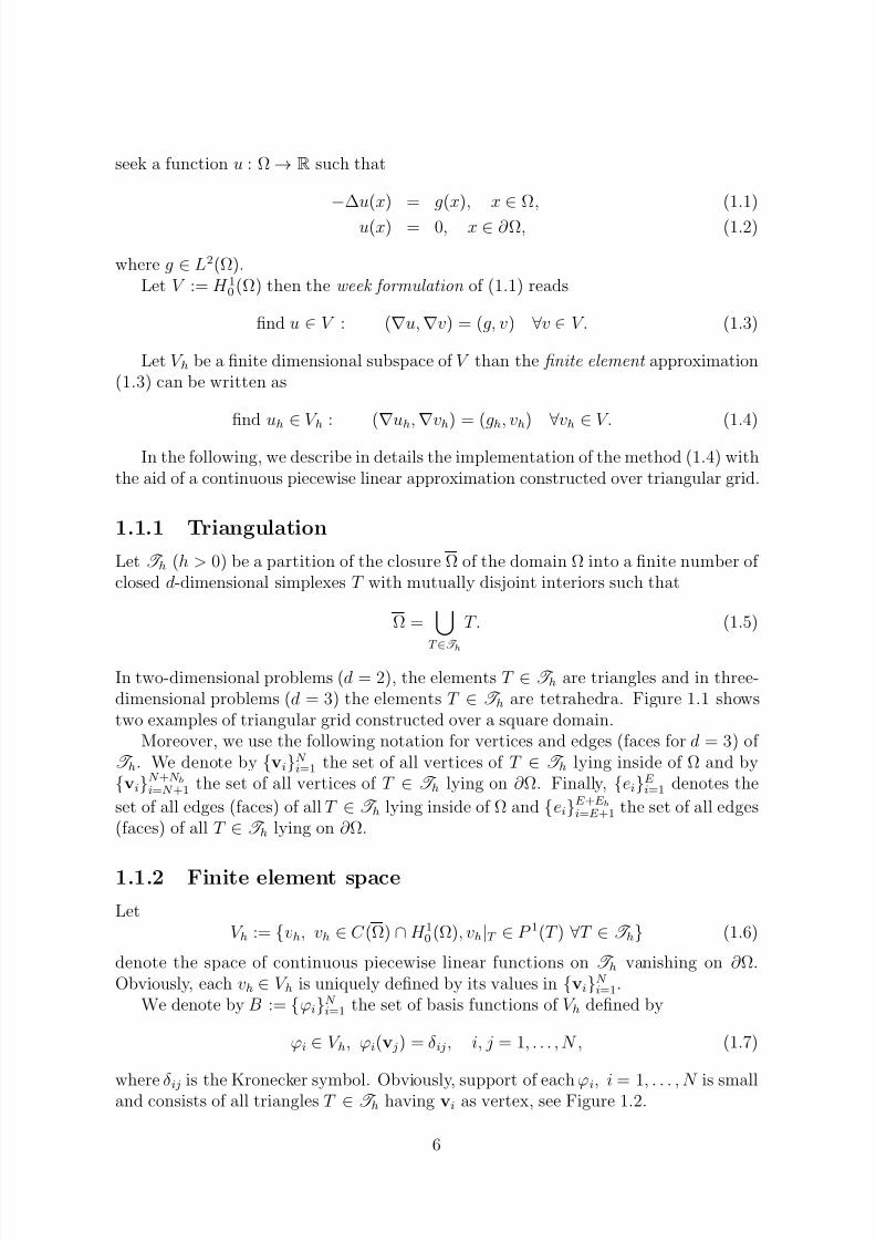
Let T h (h > 0) be a partition of the closure Ω of the domain Ω into a finite number of closed d-dimensional simplexes T with mutually disjoint interiors such that
Ω =
T ∈T hT. (1.5)
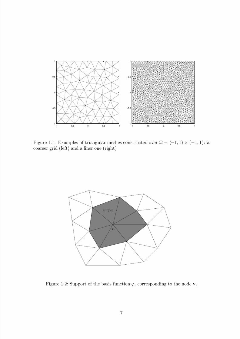
In two-dimensional problems (d = 2), the elements T ∈ T h are triangles and in three-dimensional problems (d = 3) the elements T ∈ T h are tetrahedra. Figure 1.1 showstwo examples of triangular grid constructed over a square domain.
Moreover, we use the following notation for vertices and edges (faces for d = 3) of T h. We denote by vi
N i=1 the set of all vertices of T ∈ T h lying inside of Ω and by
viN +N bi=N +1 the set of all vertices of T ∈ T h lying on ∂ Ω. Finally, ei
E i=1 denotes the
set of all edges (faces) of all T ∈ T h lying inside of Ω and eiE +E bi=E +1 the set of all edges
(faces) of all T ∈ T h lying on ∂ Ω.
1.1.2 Finite element space
LetV h := vh, vh ∈ C (Ω) ∩ H 10 (Ω), vh|T ∈ P 1(T ) ∀T ∈ T h (1.6)
denote the space of continuous piecewise linear functions on T h vanishing on ∂ Ω.Obviously, each vh ∈ V h is uniquely defined by its values in vi
N i=1.
We denote by B := ϕiN i=1 the set of basis functions of V h defined by
ϕi ∈ V h, ϕi(v j) = δ ij, i, j = 1, . . . , N , (1.7)
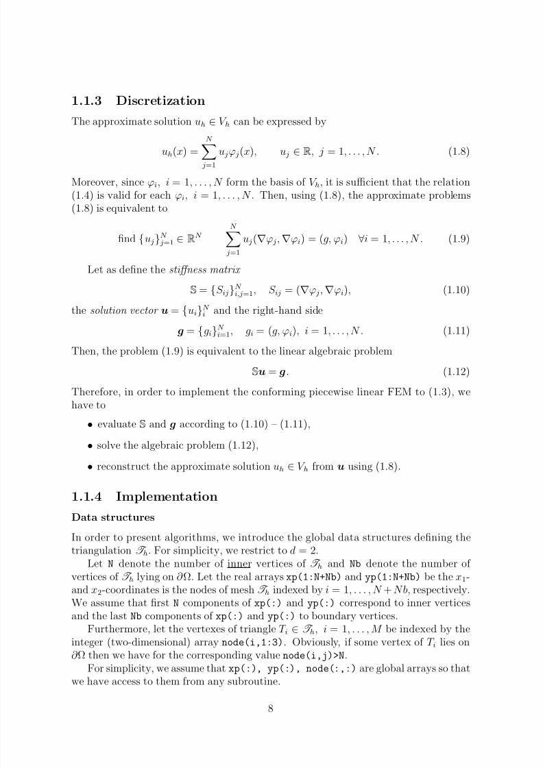
where δ ij is the Kronecker symbol. Obviously, support of each ϕi, i = 1, . . . , N is smalland consists of all triangles T ∈ T h having vi as vertex, see Figure 1.2.
6
7/23/2019 FEM Implement
http://slidepdf.com/reader/full/fem-implement 7/51
-1
-0.5
0
0.5
1
-1 -0.5 0 0.5 1
-1
-0.5
0
0.5
1
-1 -0.5 0 0.5 1
Figure 1.1: Examples of triangular meshes constructed over Ω = (−1, 1) × (−1, 1): acoarser grid (left) and a finer one (right)
vi
suppϕi
Figure 1.2: Support of the basis function ϕi corresponding to the node vi
7
7/23/2019 FEM Implement
http://slidepdf.com/reader/full/fem-implement 8/51
1.1.3 Discretization
The approximate solution uh ∈ V h can be expressed by
uh(x) =N
j=1
u jϕ j(x), u j ∈ R, j = 1, . . . , N . (1.8)
Moreover, since ϕi, i = 1, . . . , N form the basis of V h, it is sufficient that the relation(1.4) is valid for each ϕi, i = 1, . . . , N . Then, using (1.8), the approximate problems(1.8) is equivalent to
find u jN j=1 ∈ RN
N j=1
u j(∇ϕ j, ∇ϕi) = (g, ϕi) ∀i = 1, . . . , N . (1.9)
Let as define the stiffness matrix
S = S ijN i,j=1, S ij = (∇ϕ j, ∇ϕi), (1.10)
the solution vector u = uiN i and the right-hand side
g = giN i=1, gi = (g, ϕi), i = 1, . . . , N . (1.11)
Then, the problem (1.9) is equivalent to the linear algebraic problem
Su = g . (1.12)
Therefore, in order to implement the conforming piecewise linear FEM to (1.3), we
have to
• evaluate S and g according to (1.10) – (1.11),
• solve the algebraic problem (1.12),
• reconstruct the approximate solution uh ∈ V h from u using (1.8).
1.1.4 Implementation
Data structures
In order to present algorithms, we introduce the global data structures defining thetriangulation T h. For simplicity, we restrict to d = 2.
Let N denote the number of inner vertices of T h and Nb denote the number of vertices of T h lying on ∂ Ω. Let the real arrays xp(1:N+Nb) and yp(1:N+Nb) be the x1-and x2-coordinates is the nodes of mesh T h indexed by i = 1, . . . , N + Nb, respectively.We assume that first N components of xp(:) and yp(:) correspond to inner verticesand the last Nb components of xp(:) and yp(:) to boundary vertices.
Furthermore, let the vertexes of triangle T i ∈ T h, i = 1, . . . , M be indexed by theinteger (two-dimensional) array node(i,1:3). Obviously, if some vertex of T i lies on∂ Ω then we have for the corresponding value node(i,j)>N.
For simplicity, we assume that xp(:), yp(:), node(:,:) are global arrays so thatwe have access to them from any subroutine.
8
7/23/2019 FEM Implement
http://slidepdf.com/reader/full/fem-implement 9/51
vi
v j
Dij
suppϕi
suppϕi
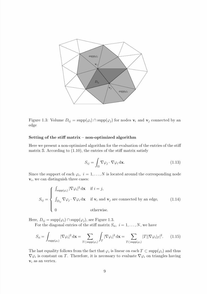
Figure 1.3: Volume Dij = supp(ϕi) ∩ supp(ϕ j) for nodes vi and v j connected by anedge
Setting of the stiff matrix – non-optimized algorithm
Here we present a non-optimized algorithm for the evaluation of the entries of the stiff matrix S. According to (1.10), the entries of the stiff matrix satisfy
S ij =
Ω
∇ϕ j · ∇ϕi dx. (1.13)
Since the support of each ϕi, i = 1, . . . , N is located around the corresponding nodevi, we can distinguish three cases:
S ij =
supp(ϕi)
|∇ϕi|2 dx if i = j,
Dij∇ϕ j · ∇ϕi dx if vi and v j are connected by an edge,
0 otherwise.
(1.14)
Here, Dij = supp(ϕi) ∩ supp(ϕ j), see Figure 1.3.
For the diagonal entries of the stiff matrix S ii, i = 1, . . . , N , we have
S ii =
supp(ϕi)
|∇ϕi|2 dx =
T ⊂supp(ϕi)
T
|∇ϕi|2 dx =
T ⊂supp(ϕi)
|T ||∇ϕi|T |2. (1.15)
The last equality follows from the fact that ϕi is linear on each T ⊂ supp(ϕi) and thus
∇ϕi is constant on T . Therefore, it is necessary to evaluate ∇ϕi on triangles havingvi as an vertex.
9
7/23/2019 FEM Implement
http://slidepdf.com/reader/full/fem-implement 10/51
[x1, y1]
[x2, y2]
[x3, y3]
ϕ
ϕ(x1, y1) = 1
T
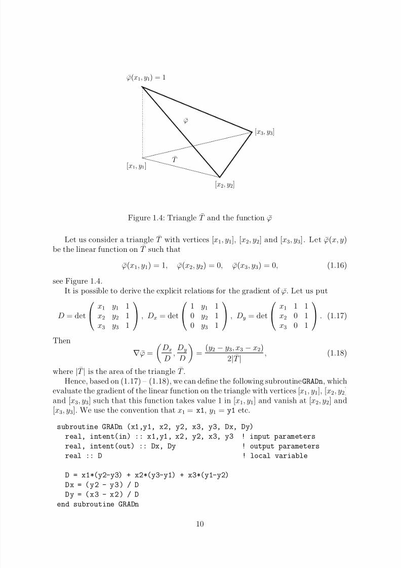
Figure 1.4: Triangle T and the function ϕ
Let us consider a triangle T with vertices [x1, y1], [x2, y2] and [x3, y3]. Let ϕ(x, y)be the linear function on T such that
ϕ(x1, y1) = 1, ϕ(x2, y2) = 0, ϕ(x3, y3) = 0, (1.16)
see Figure 1.4.It is possible to derive the explicit relations for the gradient of ϕ. Let us put
D = det
x1 y1 1x2 y2 1x3 y3 1
, Dx = det
1 y1 10 y2 10 y3 1
, Dy = det
x1 1 1x2 0 1x3 0 1
. (1.17)
Then
∇ϕ =
Dx
D ,
Dy
D
=
(y2 − y3, x3 − x2)
2|T | , (1.18)
where |T | is the area of the triangle T .Hence, based on (1.17) – (1.18), we can define the following subroutine GRADn, which
evaluate the gradient of the linear function on the triangle with vertices [ x1, y1], [x2, y2]
and [x3, y3] such that this function takes value 1 in [x1, y1] and vanish at [x2, y2] and[x3, y3]. We use the convention that x1 = x1, y1 = y1 etc.
subroutine GRADn (x1,y1, x2, y2, x3, y3, Dx, Dy)
real, intent(in) :: x1,y1, x2, y2, x3, y3 ! input parameters
real, intent(out) :: Dx, Dy ! output parameters
real :: D ! local variable
D = x1*(y2-y3) + x2*(y3-y1) + x3*(y1-y2)
Dx = (y2 - y3) / D
Dy = (x3 - x2) / Dend subroutine GRADn
10
7/23/2019 FEM Implement
http://slidepdf.com/reader/full/fem-implement 11/51
[x0, y0]
[x1, y1]
[x2, y2]
[x3, y3]
[x4, y4][x5, y5]
[x6, y6]
[xi, yi]
[x j , y j]
[xk, yk]
[xl, yl]
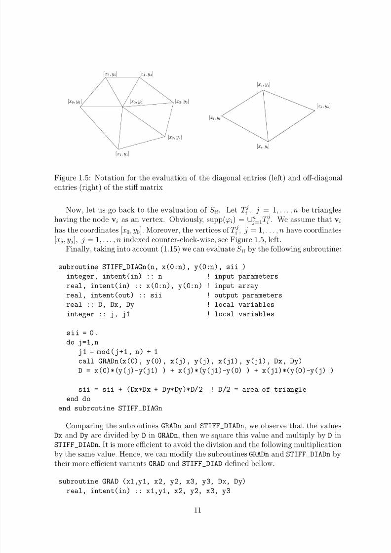
Figure 1.5: Notation for the evaluation of the diagonal entries (left) and off-diagonalentries (right) of the stiff matrix
Now, let us go back to the evaluation of S ii. Let T ji , j = 1, . . . , n be triangleshaving the node vi as an vertex. Obviously, supp(ϕi) = ∪n
j=1T ji . We assume that vi
has the coordinates [x0, y0]. Moreover, the vertices of T ji , j = 1, . . . , n have coordinates[x j, y j], j = 1, . . . , n indexed counter-clock-wise, see Figure 1.5, left.
Finally, taking into account (1.15) we can evaluate S ii by the following subroutine:
subroutine STIFF_DIAGn(n, x(0:n), y(0:n), sii )
integer, intent(in) :: n ! input parameters
real, intent(in) :: x(0:n), y(0:n) ! input array
real, intent(out) :: sii ! output parameters
real :: D, Dx, Dy ! local variables
integer :: j, j1 ! local variables
sii = 0.
do j=1,n
j1 = mod(j+1, n) + 1
call GRADn(x(0), y(0), x(j), y(j), x(j1), y(j1), Dx, Dy)
D = x(0)*(y(j)-y(j1) ) + x(j)*(y(j1)-y(0) ) + x(j1)*(y(0)-y(j) )
sii = sii + (Dx*Dx + Dy*Dy)*D/2 ! D/2 = area of triangleend do
end subroutine STIFF_DIAGn
Comparing the subroutines GRADn and STIFF_DIADn, we observe that the valuesDx and Dy are divided by D in GRADn, then we square this value and multiply by D inSTIFF_DIADn. It is more efficient to avoid the division and the following multiplicationby the same value. Hence, we can modify the subroutines GRADn and STIFF_DIADn bytheir more efficient variants GRAD and STIFF_DIAD defined bellow.
subroutine GRAD (x1,y1, x2, y2, x3, y3, Dx, Dy)real, intent(in) :: x1,y1, x2, y2, x3, y3
11
7/23/2019 FEM Implement
http://slidepdf.com/reader/full/fem-implement 12/51
real, intent(out) :: Dx, Dy
Dx = (y2 - y3)
Dy = (x3 - x2)
end subroutine GRAD
and
subroutine STIFF_DIAG( n, x, y, sii )
integer, intent(in) :: n
real, intent(in) :: x(0:n), y(0:n)
real, intent(out) :: sii
real :: D, Dx, Dy ! local variables
integer :: j, j1sii = 0.
do j=1,n
j1 = mod(j+1, n) + 1
call GRAD(x(0), y(0), x(j), y(j), x(j1), y(j1), Dx, Dy)
D = x(0)*(y(j)-y(j1) ) + x(j)*(y(j1)-y(0) ) + x(j1)*(y(0)-y(j) )
sii = sii + (Dx*Dx + Dy*Dy)/D/2 ! D/2 = area of triangle
end do
end subroutine STIFF_DIAG
Moreover, we have to evaluate the off diagonal terms of the stiff matrix, i.e., S ijwhere vi and v j are connected by an edge of T h. We denote the coordinates of verticesof triangles sharing the edge viv j according to Figure 1.5, right. The we define thesubroutine fro the evaluation of the off-diagonal term of the stiff matrix:
subroutine STIFF_OFFDIAG(xi, yi, xj, yj, xk, yk, xl, yl, sij )
real, intent(in) :: xi, yi, xj, yj, xk, yk, xl, yl
real, intent(out) :: sij
real :: D, Dx, Dy ! local variables
sij = 0.
call GRAD(xi, yi, xk, yk, xj, yj, Dx, Dy)
D = xi*(yk-yj) + xk*(yj-yi) + xj*(yi-yk)
sij = sij + (Dx*Dx + Dy*Dy)/D/2 ! D/2 = area of triangle
call GRAD(xi, yi, xj, yj, xl, yl, Dx, Dy)
D = xi*(yj-yl) + xj*(yl-yi) + xl*(yi-yj)
sij = sij + (Dx*Dx + Dy*Dy)/D/2 ! D/2 = area of triangle
end subroutine STIFF_OFFDIAG
Finally, in order to evaluate all entries of the stiff matrix S we should call either
subroutine STIFF_DIAG or STIFF_OFFDIAG for all S ij = 0. However, it requires asetting of the appropriate data structures, namely some link to the nodes connected
12
7/23/2019 FEM Implement
http://slidepdf.com/reader/full/fem-implement 13/51
by an edge to a given node (see 1.5, left) and some link between elements sharing anface (see 1.5, right.) Since we are going to introduce better algorithm in the followingsection, we skip this one.
Setting of the stiff matrix – optimized algorithm
We can notice that when we evaluate all non-vanishing terms of matrix S, we callsubroutine GRAD for each T ∈ T h several times. It is more efficient to go over allT ∈ T h only once time. This means that we compute the gradients of all possiblelinear functions on T vanishing in two vertices of T and equal to 1 in the rest node.Then we evaluate the corresponding entries of the stiff matrix.
Here we introduce more efficient algorithm for the evaluation of S. It evaluatesall entries of S which correspond to inner vertices of T h given by (1.10). First, we
define a subroutine, which evaluate the gradient of three possible restrictions of thetest functions on the given triangle.
subroutine GRADIENTS( x, y, Dphi )
real, intent(in) :: x(1:3), y(1:3)
real, intent(out) :: Dphi(1:3, 1:2)
! Dphi(i,j) = derivative of i-th function with respect x_j
Dphi(1,1) = y(2) - y(3)
Dphi(1,2) = x(3) - x(2)
Dphi(2,1) = y(3) - y(1)
Dphi(2,2) = x(1) - x(3)
Dphi(3,1) = y(1) - y(2)
Dphi(3,2) = x(2) - x(1)
end subroutine GRADIENTS
Then we have the following subroutine for the evaluation of all entries of S. Let usrecall that t xp(:), yp(:), node(:,:) are global arrays storing the coordinates of vertices and the indexes of vertices of triangles, see begin of Section 1.1.4. Hence, we
have access to them from the subroutines without their specification as input parame-ters.
subroutine STIFF(M, N, S )
integer, intent(in) :: M ! = number of triangles of triangulation
integer, intent(in) :: N ! = number of vertices of triangulation
real, dimension(1:N, 1:N), intent(out) :: S ! = stiff matrix
real :: Dphi(1:3, 1:2) , D ! local variables
integer :: i,j,ki, kj
S(1:N, 1:N) = 0
13
7/23/2019 FEM Implement
http://slidepdf.com/reader/full/fem-implement 14/51
do k=1,M
x(1:3) = xp(node(k, 1:3) )
y(1:3) = yp(node(k, 1:3) )
D = x(1)*(y(2)-y(3)) + x(2)*(y(3)-y(1)) + x(3)*(y(1)-y(2))
call GRADIENT( x(1:3), y(1:3), Dphi(1:3, 1:2) )
do ki=1,3
i = node(k,ki)
if( i <= N) then !! inner vertex?
do kj=1,3
j = node(k,kj)
if( i <= N) then !! inner vertex?
S(i,j) = S(i,j) + (Dphi(ki,1)* Dphi(kj,1) &
+ Dphi(ki,2)* Dphi(kj,2) )/D/2endif
enddo
endif
enddo
enddo
end subroutine STIFF
Remark 1 The subroutine STIFF evaluate only entries of the stiff matrix correspond-ing to the inner vertices of T h. It is assured by two if then conditions in subroutine
STIFF. If more general boundary condition than (1.2) is given also the entries corre-sponding to the boundary vertices of T h has to be evaluated. In this case, N denotes the number of all vertices including the boundary ones, see Section 1.1.5. Moreover,we can simply remove both if then conditions in subroutine STIFF.
Setting of the right-hand side
Here we present an algorithm which evaluate the entries of the vector g given by (1.11).Let i = 1, . . . , N , we have
gi = (g, ϕi) = T ⊂supp(ϕi) T g ϕi dx, (1.19)
where supp(ϕi) is shown in Figure 1.2. Generally, the integrals in (1.19) are evaluatedwith the aid of a numerical quadratures, which are discussed in Section 1.5. Since weconsidered in this section the piecewise linear approximation, we will consider only thefollowing simple quadrature rule
T
g(x) ϕ(x) dx ≈ 1
3|T |
3l=1
ϕ(xl)g(xl), (1.20)
where xl, l = 1, 2, 3 are the vertices of an triangle T ∈ T
h. This quadrature ruleintegrate exactly the linear function, hence it has the first order of accuracy.
14
7/23/2019 FEM Implement
http://slidepdf.com/reader/full/fem-implement 15/51
The application of (1.19) for the evaluation of (1.20) leads to a very simple relationsince ϕi(x0, y0) = 1 and ϕi(xl, yl) = 1, l = 1, . . . , n, see Figure 1.5, left. Then we have
gi ≈ 13
meas(supp(ϕi))g(vi), i = 1, . . . , N (1.21)
where vi, i = 1, . . . , N are inner vertices of T h.Finally, let us note that the numerical quadrature (1.20) is not sufficiently accurate
generally.
Solution of the linear algebraic system (1.12)
Once we have evaluated the entries of matrix S and vector g, we have to solve thelinear algebraic system (1.12). In the case of the Laplace problem (1.1) the situation
is very simple. First we introduce the following term
Definition 1 Let T h be a mesh of Ω. Let T and T ′ be a pair of triangles from T h shar-ing an edge viv j. Let vi, v j, vk and v j, vi, vl be the vertices of T and T ′, respectively.We denote by SumAngles(T, T ′) the sum of angles of T and T ′ adjacent to vertices vk
and vl, respectively. We say that T h is of the Delaunay type if SumAngles(T, T ′) ≤ π for each pair of triangles T, T ′ from T h sharing an edge.
It is possible to show that if T h is of Delaunay type then the corresponding stiff matrix S is symmetric and diagonally dominant. In this case in fact arbitrary director iterative solver can be used with success for the solution of (1.12).
Reconstruction of the approximate solution
Once we have found the vector u which is the solution of (1.12), we will reconstructthe piecewise linear function uh ∈ V h from u using (1.8). However, in practice we neednot know an explicit relation for uh. Usually, we require a visualization of the solutionand/or an evaluation of some characteristics. The basic visualization techniques arementioned in Section 1.6.
1.1.5 Treatment of general boundary conditions
In the previous sections, the homogeneous Dirichlet boundary condition was considered.However, in practice, more general boundary conditions have to be taken into account.
Let Ω be a bounded polygonal domain in Rd, d = 2, 3, with a boundary ∂ Ω whichconsists of two disjoint parts ∂ ΩD and ∂ ΩN . We seek find a function u : Ω → R suchthat
−∆u(x) = g(x), x ∈ Ω, (1.22)
u(x) = uD(x), x ∈ ∂ ΩD, (1.23)
∇u(x) · n = gN (x), x ∈ ∂ ΩD, (1.24)
where g ∈ L2(Ω), gN ∈ L2(∂ Ω) and uD is a trace of some u∗ ∈ H 1(Ω).
15
7/23/2019 FEM Implement
http://slidepdf.com/reader/full/fem-implement 16/51
LetV := v ∈ H 1(Ω), v|∂ ΩD
= 0 in the sense of traces (1.25)
then the week formulation of (1.22) – (1.24) reads
find u ∈ H 1(Ω) : u − u∗ ∈ V, (1.26)
(∇u, ∇v) = (g, v) + (gN , v)L2(∂ ΩN ) ∀v ∈ V .
Let T h be a mesh reflecting the ∂ Ω consists of two disjoint parts ∂ ΩD and ∂ ΩN . LetX h be a finite dimensional subspace of H 1(Ω) constructed over mesh T h and V h ⊂ X hits subspace such that vh|∂ ΩD
= 0 ∀vh ∈ V h. The finite element approximation (1.26)can be written as
find uh ∈ X h : (uh − uD, vh)L2(∂ ΩD) = 0 ∀vh ∈ X h, (1.27)
(∇uh, ∇vh) = (g, vh) + (gN , vh)L2(∂ ΩN ) ∀vh ∈ V h.
The numerical implementation of (1.27) is more complicated than the implementa-tion of (1.4). In this place we skip the evaluation of the boundary integral on the righthand side of (1.27) and refer to Section 1.4.6. We focus on the assuring of the Dirichletboundary condition on ∂ ΩD.
We use the following notation for vertices of T h which differs from the notationintroduced in the previous sections. We denote by vi
N i=1 a set of all vertices of
T ∈ T h lying inside of Ω or on ∂ ΩN and by viN +N bi=N +1 a set of all vertices of T ∈ T h
lying on ∂ ΩD.
Similarly as in the previous, we restrict to the piecewise linear approximations.Therefore, each function from X h is uniquely given by its values in vi
N +N bi=1 and each
function from V h is uniquely given by its values in viN i=1 . We denote by ϕi ∈ X h the
basis functions corresponding to vi, i = 1, . . . , N + N b given by
ϕi ∈ X h, ϕi(v j) = δ ij, i, j = 1, . . . , N + N b. (1.28)
First, we introduce a piecewise linear approximation of uD from the boundarycondition. We define a function uD,h ∈ X h \ V h by
(uD,h − uD, vh)L2(∂ ΩD) = 0 ∀vh ∈ X h \ V h. (1.29)
Such uD,h can be simply constructed since X h is a finite dimensional spaces and then(1.29) represents a system of linear algebraic equations. Namely, we have
uD,h(x) =
N b j=N +1
uD,jϕi(x), (1.30)
therefore, we have from (1.29) – (1.30) the following system of the linear algebraicequations
N b j=N +1
uD,j(ϕ j, ϕi)L2(∂ ΩD) = (uD, ϕi)L2(∂ ΩD), i = N + 1, . . . , N b. (1.31)
16
7/23/2019 FEM Implement
http://slidepdf.com/reader/full/fem-implement 17/51
The evaluation of terms (ϕ j , ϕi)L2(∂ ΩD), i ,j = N + 1, . . . , N b is simple since these termsare non-vanishing only if vi and vi are connected by an edge on ∂ ΩD. Moreover, theevaluation of (uD, ϕi)
L
2
(∂ ΩD), i = N + 1, . . . , N b reduces to an integration over two
edges on ∂ ΩD having vi as an end-point.The solution of the (1.27) can be written in the form
uh(x) =N
j=1
u jϕi(x) +
N b j=N +1
uD,jϕi(x) =N
j=1
u jϕi(x) + uD,h, (1.32)
where the coefficients uD,j , j = N + 1, . . . , N b are known and the coefficients u j, j =1, . . . , N are unknown. Inserting (1.32) into (1.27) and putting vh := ϕi, we have
N j=1
u j(∇ϕ j , ∇ϕi) = (g, vh) + (gN , vh)L2(∂ ΩN ) − (∇uD,h, ∇ϕi), i = 1, . . . , N ,
which is very close to the problem (1.10), where the right-hand-side contains addition-ally terms arising from the Dirichlet and the Neumann boundary conditions. Moreover,symbol N has little different meanings in (1.10) and in (1.33), in the former case denotesthe number of interior vertices, in the latter case the number of inner and “Dirichlet”nodes. However, all subroutines presented in Section 1.1.4 can be employed with thisminor changes.
1.2 General FE solution of the model problemIn Section 1.1 we described the implementation of the conforming piecewise linear finiteelement approximation of problem (1.1) – (1.2). Here we consider a higher degree of polynomial approximation. The implementation is more complicated since the gradientof test function is not constant over T ∈ T h.
It is more comfortable employ the concept of the reference element. This approachallows us to deal with more general elements than triangles, e.g., quadrilaterals, curvi-linear elements, etc.
1.2.1 Definition of reference elementsIn this lecture notes, we consider
• the reference simplex (triangle for d = 2 and tetrahedron for d = 3)
T t :=
x = (x1, . . . , xd)), xi ≥ 0, i = 1, . . . , d ,
di=1
xi ≤ 1
(2.33)
• the reference hexagon (square for d = 2 and cube for d = 3)
T q := x = (x1, . . . , xd)), 0 ≤ xi ≤ 1, i = 1, . . . , d , . (2.34)
17
7/23/2019 FEM Implement
http://slidepdf.com/reader/full/fem-implement 18/51
v1 = [0; 0] v2 = [1; 0]
v3 = [1; 1]v4 = [0; 1]
e1
e2
e3
e4
T q
v1 = [0; 0] v2 = [1; 0]
v3 = [0; 1]
e1
e2e3
T t
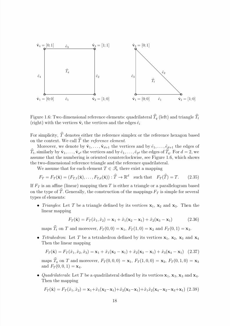
Figure 1.6: Two dimensional reference elements: quadrilateral T q (left) and triangle T t(right) with the vertices vi the vertices and the edges ei
For simplicity, T denotes either the reference simplex or the reference hexagon basedon the context. We call T the reference element .
Moreover, we denote by v1, . . . , vd+1 the vertices and by e1, . . . , ed+1 the edges of T t, similarly by v1, . . . , vsd the vertices and by e1, . . . , e2d the edges of T q. For d = 2, weassume that the numbering is oriented counterclockwise, see Figure 1.6, which showsthe two-dimensional reference triangle and the reference quadrilateral.
We assume that for each element T ∈ T h there exist a mapping
F T = F T (x) = (F T,1(x), . . . , F T,d(x)) : T → Rd such that F T ( T ) = T . (2.35)
If F T is an affine (linear) mapping then T is either a triangle or a parallelogram based
on the type of T . Generally, the construction of the mappings F T is simple for severaltypes of elements:
• Triangles : Let T be a triangle defined by its vertices x1, x2 and x3. Then thelinear mapping
F T (x) = F T (x1, x2) = x1 + x1(x2 − x1) + x2(x3 − x1) (2.36)
maps T t on T and moreover, F T (0, 0) = x1, F T (1, 0) = x2 and F T (0, 1) = x3.
• Tetrahedron : Let T be a tetrahedron defined by its vertices x1, x2, x3 and x4
Then the linear mapping
F T (x) = F T (x1, x2, x3) = x1 + x1(x2 − x1) + x2(x3 − x1) + x3(x4 − x1) (2.37)
maps T q on T and moreover, F T (0, 0, 0) = x1, F T (1, 0, 0) = x2, F T (0, 1, 0) = x3
and F T (0, 0, 1) = x4.
• Quadrilaterals : Let T be a quadrilateral defined by its vertices x1, x2, x3 and x4.Then the mapping
F T (x) = F T (x1, x2) = x1+x1(x2−x1)+x2(x3−x1)+x1x2(x4−x2−x3+x1) (2.38)
18
7/23/2019 FEM Implement
http://slidepdf.com/reader/full/fem-implement 19/51
x2
x2,3
x3
x1
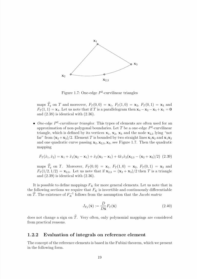
Figure 1.7: One-edge P 2-curvilinear triangles
maps T q on T and moreover, F T (0, 0) = x1, F T (1, 0) = x2, F T (0, 1) = x3 andF T (1, 1) = x4. Let us note that if T is a parallelogram then x4 − x2 − x3 + x1 = 0and (2.38) is identical with (2.36).
• One-edge P 2-curvilinear triangles : This types of elements are often used for anapproximation of non-polygonal boundaries. Let T be a one-edge P 2-curvilineartriangle, which is defined by its vertices x1, x2, x3 and the node x2,3 lying “notfar” from (x2 + x3)/2. Element T is bounded by two straight lines x1x2 and x1x2
and one quadratic curve passing x2, x2,3, x3, see Figure 1.7. Then the quadratic
mapping
F T (x1, x2) = x1 + x1(x2 − x1) + x2(x3 − x1) + 4x1x2(x2,3 − (x2 + x3)/2) (2.39)
maps T q on T . Moreover, F T (0, 0) = x1, F T (1, 0) = x2, F T (0, 1) = x3 andF T (1/2, 1/2) = x2,3. Let us note that if x2,3 = (x2 + x3)/2 then T is a triangleand (2.39) is identical with (2.36).
It is possible to define mappings F K for more general elements. Let us note that inthe following sections we require that F K is invertible and continuously differentiable
on T . The existence of F −1
K follows from the assumption that the Jacobi matrix
J F T (x) := D
DxF T (x) (2.40)
does not change a sign on T . Very often, only polynomial mappings are consideredfrom practical reasons.
1.2.2 Evaluation of integrals on reference element
The concept of the reference elements is based in the Fubini theorem, which we presentin the following form.
19
7/23/2019 FEM Implement
http://slidepdf.com/reader/full/fem-implement 20/51
Theorem 1 (Fubini theorem) Let T be the image of F T ( T ) where T is the reference element and F T is the continuously differentiable mapping. Let f (x) : T → R be an
integrable function defined on T . We define the function ˆf : T →
R
by ˆf (x) = f (x)where x = F T (x). Then
T
f (x) dx =
T
f (x)| det J F T (x)| dx, (2.41)
where J F T is the Jacobi matrix of F T .
Let us note that if F T is a linear mapping (i.e., T is an simplex or a parallelogram)then J F is a constant matrix and | det J F T | = 2|T |, where |T | denotes the d-dimensionalLebesgue measure of T .
Theorem 1 gives us a tool for the evaluation of the various type of integrals in the
implementation of finite element and discontinuous Galerkin methods. Instead of inte-gration over T we integrate over T which is generally more easy. This is demonstratedin the following paragraphs.
Let T ∈ T h and ϕ be a function defined on T . Our aim is to compute T
∂ϕ(x)
∂xidx. (2.42)
Let ϕ : T → R be defined as usual by ϕ(x) = ϕ(x) where x = F T (x),
F T = (F T,1, . . . , F T,d)
and T = F T ( T ). Moreover, we have x = F −1T (x) where
F −1T = (F −1T,1, . . . , F −1T,d)
is the inverse mapping of F T . With the aid of Theorem 1 and the chain rule, we have T
∂
∂xi
ϕ(x) dx =
T
∂
∂xi
ϕ(x)| det J F T (x)| dx (2.43)
=
T
dk=1
∂ ϕ(x)
∂ xk
∂ xk
∂xi| det J F T (x)| dx =
T
dk=1
∂ ϕ(x)
∂ xk
∂F −1T,k
∂xi| det J F T (x)| dx.
Therefore, we have to evaluate the partial derivative of F −1T . It is possible to use the
following determination. Let i, k = 1, . . . , d, then
xk = F T,k(F −1T (x)), | ∂
∂xi
∂
∂xi
xk = ∂
∂xi
F T,k(F −1T (x)),
δ ik =dl=1
∂F T,k∂ xl
∂F −1T,l
∂xi
,
δ ik =
dl=1
(J F T )kl (J F −1T )li, (2.44)
20
7/23/2019 FEM Implement
http://slidepdf.com/reader/full/fem-implement 21/51
where (J F T )kl, k , l = 1, . . . , d and (J F −1T
)li, l , i = 1, . . . , d denote entries of the Jacobi
matrices J F T and J F −1T , respectively. The relation (2.44) implies
I = J F T J F −1T =⇒ J F −1T
= (J F T )−1. (2.45)
Therefore, instead of evaluation of the Jacobi matrix of F −1T it is sufficient to evaluate(J F T )
−1 = the inversion of J F T . This is simple since J F T is (usually) 2 × 2 or 3 × 3matrix.
Therefore, from (2.43) and (2.45) we have T
∂
∂xi
ϕ(x) dx =
T
dk=1
∂ ϕ(x)
∂ xk(J F T (x)−1)ki| det J F T (x)| dx (2.46)
= T
dk=1
∂ ϕ(x)∂ xk
(J F T (x)−T)ik| det J F T (x)| dx
=
T
J F T (x)−T ∇ϕ(x)
i
| det J F T (x)| dx,
where J −TF T is the transposed matrix to J −1F T
, (J −TF T ∇ϕ)i denotes the i-th component
of vector J −TF T ∇ϕ arising from the matrix-vector product of J −TF T
by ∇ϕ and ∇ is thereference gradient operator given by
∇ := ∂
∂ x1
, . . . , ∂
∂ xd . (2.47)
In the same manner it is possible to derive, e.g., T
∂ϕa(x)
∂xi
∂ϕb(x)
∂x jdx =
T
J F T (x)−T ∇ϕa(x)
i
J F T (x)−T ∇ϕb(x)
j
| det J F T (x)| dx
(2.48)or more simply
T
∂ϕa
∂xi
∂ϕb
∂x jdx =
T
J −TF T
∇ϕa
i
J −TF T
∇ϕb
j
| det J F T | dx (2.49)
which is type of integral appearing in the evaluation of the stiff matrix.
1.2.3 Grids and functional spaces
We again consider the model Poisson problem (1.1) – (1.2), the weak formulation (1.3)and the finite element discretization (1.4). In contrast to Section 1.1, we considermore general partitions of Ω and finite element spaces. Let a grid T h be a set of non-overlapping elements T ∈ T h such that
Ω =
T ∈T hT. (2.50)
We consider two following type of grids.
21
7/23/2019 FEM Implement
http://slidepdf.com/reader/full/fem-implement 22/51
Triangular grid
Each element T ∈ T h is an images of the reference triangle (for d = 2) or the reference
tetrahedron (for d = 3) given by a polynomial mapping F T : T t → R, T ∈ T h. If F T isa linear mapping then T is a triangle (for d = 2) or a tetrahedron (for d = 3). If F T has the form (2.39) then T is an one-edge P 2-curvilinear triangle. The approximatesolution is sought in the functional space
V t,ph := vh, vh ∈ C (Ω) ∩ H 10 (Ω), vh|T F T ∈ P t,p( T t) ∀T ∈ T h, (2.51)
P t,p(ω) := z : ω → R, z (x1, . . . , xd) =
i1+...+id≤ pi1,...,id=0
ai1,...,id xi11 . . . xidd , ai1,...,id ∈ R,
where ω ⊂ Rd is an arbitrary domain Let us note that the notation vh|T F T ∈ P t,p( T t)
means that there exists a function vh ∈ P t,p( T t) such that
vh(x) = vh(F T (x)) = vh(x) ∀x ∈ T t. (2.52)
Obviously, if F T is a linear mapping then vh|T ∈ P t,p(T ). Otherwise, (e.g., T is acurvilinear triangle), vh|T ∈ P t,p(T ).
The spaces P t,p( T t), p = 1, 2, 3 can be expressed (for d = 2) as
P t,1( T t) = span1, x1, x2, (2.53)
P t,2(
T t) = span1, x1, x2, x2
1, x1x2, x22,
P t,3( T t) = span1, x1, x2, x21, x1x2, x2
2, x31, x2
1x2, x1x22, x3
2,
where spanS is the linear hull of the set S . Obviously, N t,p := dim P t,p( T t) =
( p +1)( p + 2)/2 for d = 2 and N t,p := dim P t,p( T t) = ( p +1)( p +2)( p + 3)/6 for d = 3.
Quadrilateral grids
Each element T ∈ T h is an images of the reference square (for d = 2) or the reference
cube (for d = 3) given by a polynomial mapping F T : T t → R, T ∈ T h. If F T is alinear mapping then T is a parallelogram. The approximate solution is sought in thefunctional space
V q,ph := vh, vh ∈ C (Ω) ∩ H 10 (Ω), vh|T F T ∈ P q,p( T q) ∀T ∈ T h, (2.54)
P q,p(ω) := z : ω → R, z (x1, . . . , xd) =
pi1,...,id=0
ai1,...,idxi11 . . . xidd , ai1,...,id ∈ R,
where ω ⊂ Rd is an arbitrary domain.The spaces P q,p( T q), p = 1, 2, 3 can be expressed (for d = 2) as
P q,1( T q) = span1, x1, x2, x1x2, (2.55)
P q,2(
T q) = span1, x1, x2, x1x2, x2
1, x21x2, x2
1x22, x1x2
2, x22,
P q,3( T q) = span1, x1, x2, x1x2, x2
1
, x2
1
x2, x2
1
x2
2
, x1x2
2
, x2
2
,
x31, x3
1x2, x31x2
2, x31x3
2, x21x3
2, x1x32, x3
2.
22
7/23/2019 FEM Implement
http://slidepdf.com/reader/full/fem-implement 23/51
Obviously, N q,p := dim P q,p( T q) = ( p + 1)d for d = 2, 3.Since the most of the following considerations are valid for triangular as well as
quadrilateral grids we call T h
a triangulation in both cases. Moreover, the correspond-ing reference element is denoted by T , P p( T ) the corresponding space of polynomial
functions on T with the dimension N and the corresponding finite element space isdenoted by V h.
1.2.4 Implementation
Basis of V h
Let N denote the dimension of the space V h and Bh := ϕi(x)N i=1 be its basis. Theconstruction of Bh will be discussed in Section 1.3. Here we only note that we construct
the set reference shape functions B := ϕ j , ϕ j : T → RN j=1 such that
• ϕ j(x) ∈ P p( T ), j = 1, . . . , N , N is the dimension of P p( T ).
• ϕ j(x), j = 1, . . . , N are linearly independent,
• span( B) = P p( T ).
We call B the reference basis .Moreover, in virtue of (2.51) or (2.54), the basis functions ϕi ∈ Bh satisfy: for each
T ∈T h, T ⊂ supp(ϕi) there exists a function ϕi,T ∈
ˆB such that
ϕi(x)|T = ϕi(F T (x))|T = ϕi,T (x) ∀x ∈ T , i = 1, . . . , N . (2.56)
More details are given in Section 1.3.
A use of the concept of the reference elements
Our aim is to evaluate the integrals of type
T ∂ϕi
∂xk
∂ϕ j
∂xl
dx, i, j = 1, . . . , N , k, l = 1, . . . , d , T ∈ T h, (2.57)
which appears, e.g., in the definition of the stiff matrix.A use of the approach from Section 1.1 requires an evaluation (and storing) of ∇ϕi|T
for all i = 1, . . . , N and all T ∈ T h. Let us note, that ∇ϕi|T = 0 for a lot of T ∈ T h
since supports of test functions contain only a few elements from T h.It is more efficient to employ the concept of the reference elements, namely relation
(2.49), where the integration is carried out on the reference element T .Therefore, using (2.49) and (2.57), we can evaluate (2.57) with the aid of
T
∂ϕi
∂xk
∂ϕ j
∂xl dx = T J
−TF T ∇ϕi,T k J
−TF T ∇ϕ j,T l | det J F T | dx. (2.58)
23
7/23/2019 FEM Implement
http://slidepdf.com/reader/full/fem-implement 24/51
Data structures
In order to evaluate the right-hand side of (2.58) for all i, j = 1, . . . , N , k , l =
1, . . . , d , T ∈ T h it is enough to evaluate and store the following data.
(S1) for each T ∈ T h, the determinant of the Jacobi matrix det J F T and the transposedmatrix of the inversion of the Jacobi matrix J −TF T
,
(S2) for each ϕi, i = 1, . . . N , the gradient ∇ϕi on T ,
(S3) for each pair (ϕi, T ), T ∈ T h, T ⊂ supp(ϕi), i = 1, . . . , N , an index j ∈1, . . . , N such that ϕi(F T (x))|T = ϕ j(x).
Let us note that (S1) is given by the geometry of the mesh, (S2) by the reference shape
functions and (S3) by a combination of both. However, in (S3) we have to store onlyone integer index for any acceptable pair (ϕi, T ).
1.3 Basis and shape functions
In this section we describe two possible way (among others) of the construction of basisof spaces V t,ph and V q,ph given by (2.54) and (2.52), respectively. In Section 1.3.1 wedescribe the construction of Lagrangian basis, which is easy for the determination andalso for the implementation. However, in case when we use, e.g., different degrees of
polynomial approximations at different elements (hp-methods), the efficiency of thisapproach is low. Therefore, in Section 1.3.2 we present the construction of the Lobattobasis, which is more efficient generally.
As we have already mentioned in Section 1.2.4, first we define the reference shape functions B := ϕ jN j=1 defined on the reference element T . Then the basis of V h is
generated from B. We present the construction of the shape functions for d = 2. Ford = 3, it is possible use the similar (but technically more complicated) approach.
1.3.1 The reference Lagrangian shape functions
The reference Lagrangian shape functions are defined with the aid of a set of thereference Lagrangian nodes zi = (z i,1, z i,2), i = 1, . . . , N within the reference element.
Then we simply put ϕi(z k) = δ ij, i , j = 1, . . . , N . In the following we introducethe reference Lagrangian nodes and the reference Lagrangian shape function for thereference triangle and the reference square separately.
The reference Lagrangian shape functions on the square
Definition 2 (Lagrangian nodes) Let p ≥ 1, then the Lagrangian nodes on the refer-
ence square
T q corresponding to the polynomial degree p is the set of nodes
zq,pk N q,p
k=1 , zq,pk = (z q,pk,1, z q,pk,2) (3.59)
24
7/23/2019 FEM Implement
http://slidepdf.com/reader/full/fem-implement 25/51
zq,11
zq,12
zq,13
zq,14
zq,21
zq,22
zq,23
zq,24
zq,25
zq,26
zq,27
zq,28
zq,29
zq,31
zq,32
zq,33
zq,34
zq,35
zq,36
zq,37
zq,38
ˆzq,39 ˆz
q,310 ˆz
q,311 ˆz
q,312
zq,313
zq,314
zq,315
zq,316
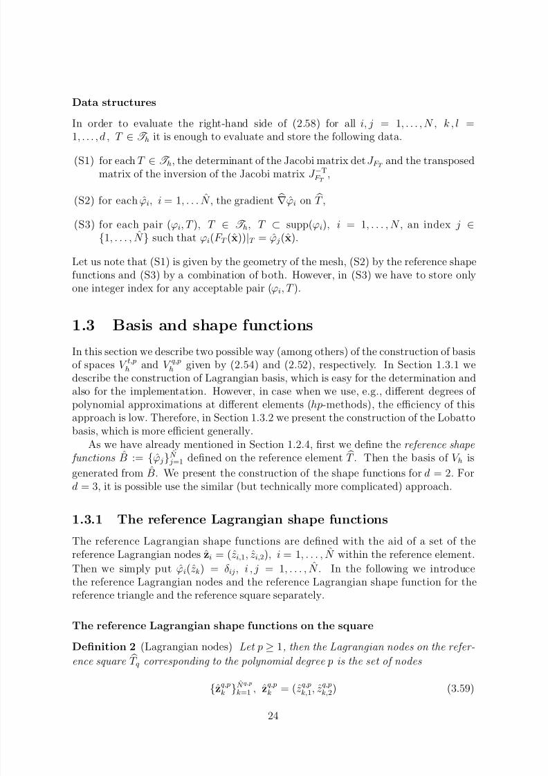
Figure 1.8: The reference Lagrangian nodes on the reference square
T q, p = 1 (left),
p = 2 (center) and p = 3 (right)
where z q,p j( p+1)+i+1,1 = i/p, z q,p j( p+1)+i+1,2 = j/p, i, j = 0, . . . , p . (3.60)
Obviously, N q,p = ( p + 1)2.
Figure 1.8 shows the Lagrangian nodes for p = 1, 2, 3. We define the reference Lagrangian shape functions ϕq,p
l N q,p
l=1 for p ≥ 1 on the reference square T q by therelation
ϕq,pl ∈ P p(
T q), ϕq,p
l (zq,pk ) = δ lk, l , k = 1, . . . , N q,p. (3.61)
It is possible to derive the following explicit relations for the Lagrangian shape functions
on the reference square T q
p = 1 ϕq,11 = (1 − λ1)(1 − λ2), ϕq,1
2 = λ1(1 − λ2), (3.62)
ϕq,13 = λ2(1 − λ1), ϕq,1
4 = λ1λ2
p = 2 ϕq,21 = 4(1 − λ1)(
1
2 − λ1)(1 − λ2)(
1
2 − λ2),
ϕq,22 = 8λ1(1 − λ1)(1 − λ2)(
1
2 − λ2),
ϕq,23 = −4λ1(
1
2 − λ1)(1 − λ2)(
1
2 − λ2),
ϕq,24 = 8(1 − λ1)(1
2 − λ1)λ2(1 − λ2),
ϕq,25 = 16λ1(1 − λ1)λ2(1 − λ2),
ϕq,26 = −8λ1(
1
2 − λ1)λ2(1 − λ2),
ϕq,27 = −4(1 − λ1)(
1
2 − λ1)λ2(
1
2 − λ2),
ϕq,28 = −8λ1(1 − λ1)λ2(
1
2 − λ2),
ϕq,29 = 4λ1(
1
2 − λ1)λ2(
1
2 − λ2),
where λ1 = x1 and λ2 = x2 are the barycentric coordinates on T q.
25
7/23/2019 FEM Implement
http://slidepdf.com/reader/full/fem-implement 26/51
zt,11
zt,12
zt,13
zt,21
zt,22
zt,23
zt,24
zt,25
zt,26
zt,31
zt,32
zt,33
zt,34
zt,35
zt,36
zt,37
ˆzt,3
8
zt,3
9
zt,310
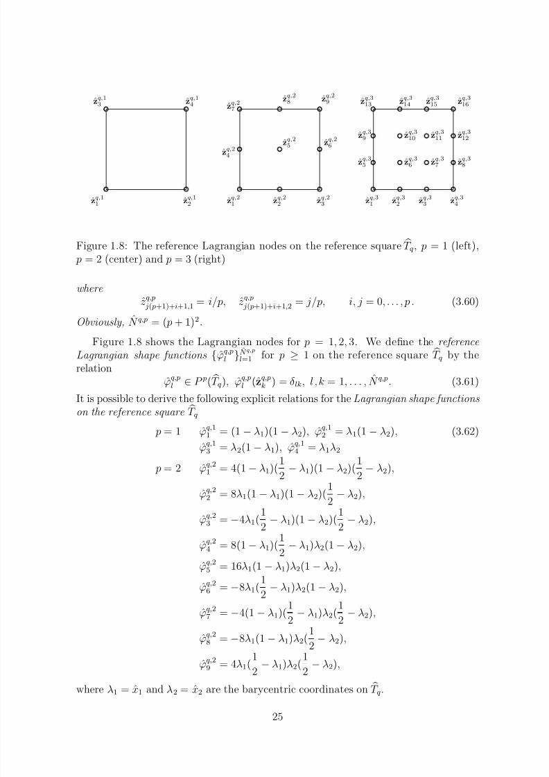
Figure 1.9: Lagrangian nodes on the reference triangle
T t, p = 1 (left), p = 2 (center)
and p = 3 (right)
The reference Lagrangian shape functions on the triangle
Definition 3 (Lagrangian nodes) Let p ≥ 1, then the reference Lagrangian nodes on
the reference triangle T t corresponding to the polynomial degree p is the set of nodes
zt,pk N t,p
k=1 , zt,pk = (z t,pk,1, z t,pk,2) (3.63)
generated by the following algorithm
k := 0 for i = 0, . . . , p for j = 0, . . . , p − i
k := k + 1z t,pk,1 = j/p,
z t,pk,2 = i/p.
(3.64)
Obviously, N t,p = ( p + 1)( p + 2)/2.
Figure 1.9 shows the Lagrangian nodes for p = 1, 2, 3. We define the reference Lagrangian shape functions ϕt,p
l N
t,p
l=1
by the relation
ϕt,pl ∈ P t,p( K t), ϕt,p
l (zt,pk ) = δ lk, l , k = 1, . . . , N t,p. (3.65)
It is possible to derive the following explicit relation for the Lagrangian shape functions on the reference triangle T t
p = 1 ϕt,11 = λ1, ϕt,1
2 = λ2, ϕt,13 = λ3, (3.66)
p = 2 ϕt,22 = λ1(2λ1 − 1), ϕt,2
2 = 4λ1λ2, ϕt,23 = λ2(2λ2 − 1),
ϕt,2
4
= 4λ2λ3, ϕt,2
5
= λ3(2λ3 − 1), ϕt,2
6
= 4λ3λ1,
26
7/23/2019 FEM Implement
http://slidepdf.com/reader/full/fem-implement 27/51
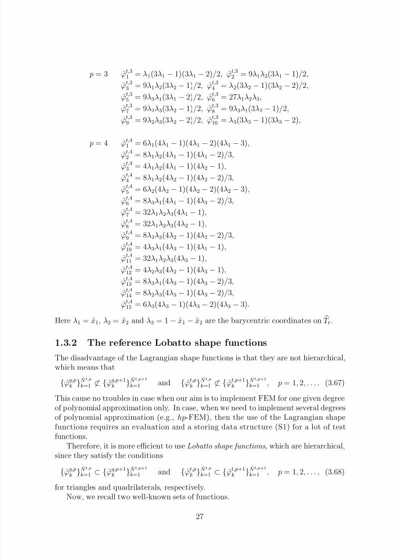
p = 3 ϕt,31 = λ1(3λ1 − 1)(3λ1 − 2)/2, ϕt,3
2 = 9λ1λ2(3λ1 − 1)/2,
ϕt,33 = 9λ1λ2(3λ2 − 1)/2, ϕt,3
4 = λ2(3λ2 − 1)(3λ2 − 2)/2,
ϕt,35 = 9λ3λ1(3λ1 − 2)/2, ϕ
t,36 = 27λ1λ2λ3,
ϕt,37 = 9λ2λ3(3λ2 − 1)/2, ϕt,3
8 = 9λ3λ1(3λ2 − 1)/2,
ϕt,39 = 9λ2λ3(3λ2 − 2)/2, ϕt,3
10 = λ3(3λ3 − 1)(3λ3 − 2),
p = 4 ϕt,41 = 6λ1(4λ1 − 1)(4λ1 − 2)(4λ1 − 3),
ϕt,42 = 8λ1λ2(4λ1 − 1)(4λ1 − 2)/3,
ϕt,43 = 4λ1λ2(4λ1 − 1)(4λ2 − 1),
ϕt,44 = 8λ1λ2(4λ2 − 1)(4λ2 − 2)/3,
ϕt,45 = 6λ2(4λ2 − 1)(4λ2 − 2)(4λ2 − 3),
ϕt,46 = 8λ3λ1(4λ1 − 1)(4λ3 − 2)/3,
ϕt,47 = 32λ1λ2λ3(4λ1 − 1),
ϕt,48 = 32λ1λ2λ3(4λ2 − 1),
ϕt,49 = 8λ2λ3(4λ2 − 1)(4λ2 − 2)/3,
ϕt,410 = 4λ3λ1(4λ3 − 1)(4λ1 − 1),
ϕt,411 = 32λ1λ2λ3(4λ3 − 1),
ϕt,412 = 4λ2λ3(4λ2 − 1)(4λ3 − 1),
ϕt,413 = 8λ3λ1(4λ3 − 1)(4λ3 − 2)/3,
ϕt,4
14 = 8λ2λ3(4λ3 − 1)(4λ3 − 2)/3,ϕt,415 = 6λ3(4λ3 − 1)(4λ3 − 2)(4λ3 − 3).
Here λ1 = x1, λ2 = x2 and λ3 = 1 − x1 − x2 are the barycentric coordinates on T t.
1.3.2 The reference Lobatto shape functions
The disadvantage of the Lagrangian shape functions is that they are not hierarchical,which means that
ϕq,pk N
t,p
k=1 ⊂ ϕq,p+1k N
t,p+1
k=1 and ϕt,pk N
t,p
k=1 ⊂ ϕt,p+1k N
t,p+1
k=1 , p = 1, 2, . . . . (3.67)
This cause no troubles in case when our aim is to implement FEM for one given degreeof polynomial approximation only. In case, when we need to implement several degreesof polynomial approximation (e.g., hp-FEM), then the use of the Lagrangian shapefunctions requires an evaluation and a storing data structure (S1) for a lot of testfunctions.
Therefore, it is more efficient to use Lobatto shape functions , which are hierarchical,since they satisfy the conditions
ϕq,pk N
t,p
k=1 ⊂ ϕq,p+1k N
t,p+1
k=1 and ϕt,pk N
t,p
k=1 ⊂ ϕt,p+1k N
t,p+1
k=1 , p = 1, 2, . . . , (3.68)
for triangles and quadrilaterals, respectively.Now, we recall two well-known sets of functions.
27
7/23/2019 FEM Implement
http://slidepdf.com/reader/full/fem-implement 28/51
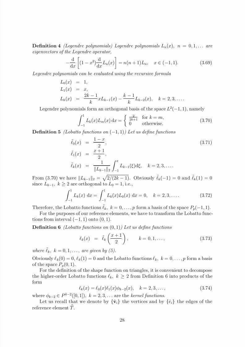
Definition 4 (Legendre polynomials) Legendre polynomials Ln(x), n = 0, 1, . . . are eigenvectors of the Legendre operator,
− ddx(1 − x2) d
dxLn(x) = n(n + 1)Ln, x ∈ (−1, 1). (3.69)
Legendre polynomials can be evaluated using the recursive formula
L0(x) = 1,
L1(x) = x,
Lk(x) = 2k − 1
k xLk−1(x) −
k − 1
k Lk−2(x), k = 2, 3, . . . .
Legendre polynomials form an orthogonal basis of the space L2(−1, 1), namely
1−1 Lk(x)Lm(x) dx = 22k+1
for k = m,
0 otherwise. (3.70)
Definition 5 (Lobatto functions on (−1, 1)) Let us define functions
ℓ0(x) = 1 − x
2 , (3.71)
ℓ1(x) = x + 1
2 ,
ℓk(x) = 1
Lk−12
x−1
Lk−1(ξ )dξ, k = 2, 3, . . . .
From (3.70) we have Lk−12 = 2/(2k − 1). Obviously ℓk(−1) = 0 and ℓk(1) = 0
since Lk−1, k ≥ 2 are orthogonal to L0 = 1, i.e., 1−1
Lk(x) dx =
1−1
Lk(x)L0(x) dx = 0, k = 2, 3, . . . . (3.72)
Therefore, the Lobatto functions ℓk, k = 0, . . . , p form a basis of the space P p(−1, 1).For the purposes of our reference elements, we have to transform the Lobatto func-
tions from interval (−1, 1) onto (0, 1).
Definition 6 (Lobatto functions on (0, 1)) Let us define functions
ℓk(x) = ℓk x + 1
2 , k = 0, 1, . . . , (3.73)
where ℓk, k = 0, 1, . . . , are given by (5).
Obviously ℓk(0) = 0, ℓk(1) = 0 and the Lobatto functions ℓk, k = 0, . . . , p form a basisof the space P p(0, 1).
For the definition of the shape function on triangles, it is convenient to decomposethe higher-order Lobatto functions ℓk, k ≥ 2 from Definition 6 into products of theform
ℓk(x) = ℓ0(x)ℓ1(x)φk−2(x), k = 2, 3, . . . , (3.74)
where φk−2 ∈ P k−2([0, 1]), k = 2, 3, . . . are the kernel functions .
Let us recall that we denote by vi the vertices and by ei the edges of thereference element T .
28
7/23/2019 FEM Implement
http://slidepdf.com/reader/full/fem-implement 29/51
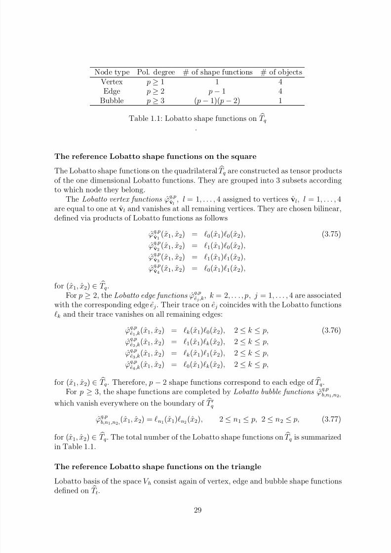
Node type Pol. degree # of shape functions # of objectsVertex p ≥ 1 1 4Edge p ≥ 2 p − 1 4
Bubble p ≥ 3 ( p − 1)( p − 2) 1
Table 1.1: Lobatto shape functions on T q.
The reference Lobatto shape functions on the square
The Lobatto shape functions on the quadrilateral
T q are constructed as tensor products
of the one dimensional Lobatto functions. They are grouped into 3 subsets according
to which node they belong.The Lobatto vertex functions ϕq,pvl
, l = 1, . . . , 4 assigned to vertices vl, l = 1, . . . , 4are equal to one at vl and vanishes at all remaining vertices. They are chosen bilinear,defined via products of Lobatto functions as follows
ϕq,pv1
(x1, x2) = ℓ0(x1)ℓ0(x2), (3.75)
ϕq,pv2
(x1, x2) = ℓ1(x1)ℓ0(x2),
ϕq,pv3
(x1, x2) = ℓ1(x1)ℓ1(x2),
ϕq,pv4
(x1, x2) = ℓ0(x1)ℓ1(x2),
for (x1, x
2) ∈ T
q.
For p ≥ 2, the Lobatto edge functions ϕq,pej ,k
, k = 2, . . . , p, j = 1, . . . , 4 are associatedwith the corresponding edge e j. Their trace on e j coincides with the Lobatto functionsℓk and their trace vanishes on all remaining edges:
ϕq,pe1,k
(x1, x2) = ℓk(x1)ℓ0(x2), 2 ≤ k ≤ p, (3.76)
ϕq,pe2,k
(x1, x2) = ℓ1(x1)ℓk(x2), 2 ≤ k ≤ p,
ϕq,pe3,k
(x1, x2) = ℓk(x1)ℓ1(x2), 2 ≤ k ≤ p,
ϕq,pe4,k
(x1, x2) = ℓ0(x1)ℓk(x2), 2 ≤ k ≤ p,
for (x1, x2) ∈ T q. Therefore, p − 2 shape functions correspond to each edge of T q.For p ≥ 3, the shape functions are completed by Lobatto bubble functions ϕq,p
b,n1,n2,
which vanish everywhere on the boundary of T ′q
ϕq,pb,n1,n2,
(x1, x2) = ℓn1(x1)ℓn2(x2), 2 ≤ n1 ≤ p, 2 ≤ n2 ≤ p, (3.77)
for (x1, x2) ∈ T q. The total number of the Lobatto shape functions on T q is summarizedin Table 1.1.
The reference Lobatto shape functions on the triangle
Lobatto basis of the space V h consist again of vertex, edge and bubble shape functionsdefined on T t.
29
7/23/2019 FEM Implement
http://slidepdf.com/reader/full/fem-implement 30/51
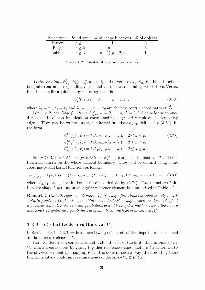
Node type Pol. degree # of shape functions # of objectsVertex p ≥ 1 1 3Edge p ≥ 2 p − 1 3
Bubble p ≥ 3 ( p − 1)( p − 2)/2 1
Table 1.2: Lobatto shape functions on T t.
Vertex functions ϕt,pv1
, ϕt,pv2
, ϕt,pv3
, are assigned to vertices v1, v2, v3. Each functionis equal to one at corresponding vertex and vanishes at remaining two vertices. Vertexfunctions are linear, defined by following formulas
ϕt,p
ˆvk(x
1, x
2) = λ
k, k = 1, 2, 3, (3.78)
where λ1 = x1, λ2 = x2 and λ3 = 1 − x1 − x2 are the barycentric coordinates on T t.For p ≥ 2, the Edge functions ϕt,p
ej ,k, k = 2, . . . , p, j = 1, 2, 3 coincide with one-
dimensional Lobatto functions on corresponding edge and vanish on all remainingedges. They can be written using the kernel functions φk−2, defined by (3.74), inthe form
ϕt,pe1,k
(x1, x2) = λ1λ2φk−2(λ2 − λ1), 2 ≤ k ≤ p, (3.79)
ϕt,pe2,k
(x1, x2) = λ2λ3φk−2(λ3 − λ2), 2 ≤ k ≤ p,
ϕt,pe3,k
(x1, x2) = λ3λ1φk−2(λ1 − λ3), 2 ≤ k ≤ p.
For p ≥ 3, the bubble shape functions ϕt,pb,n1,n2
complete the basis on T t. Thesefunctions vanish on the whole element boundary. They will be defined using affinecoordinates and kernel functions as follows
ϕt,pb,n1,n2
= λ1λ2λ3φn1−1(λ3−λ2)φn2−1(λ2−λ1), 1 ≤ n1, 1 ≤ n2, n1+n2 ≤ p−1, (3.80)
where φn1−1, φn2−1 are the kernel functions defined by (3.74). Total number of theLobatto shape functions on triangular reference element is summarized in Table 1.2.
Remark 2 On both reference domains
T q,
T t shape functions coincide on edges with
Lobatto functions ℓk, k = 0, 1, . . .. Moreover, the bubble shape functions does not affect a possible compatibility between quadrilateral and triangular meshes This allows us tocombine triangular and quadrilateral elements in one hybrid mesh, see [1].
1.3.3 Global basis functions on V h
In Sections 1.3.1 – 1.3.2, we introduced two possible sets of the shape functions definedon the reference element T .
Here we describe a construction of a global basis of the finite-dimensional spaceV h, which is carried out by gluing together reference shape functions (transformed to
the physical element by mapping F T ). It is done in such a way, that resulting basisfunctions satisfy conformity requirements of the space V h ⊂ H 1(Ω).
30
7/23/2019 FEM Implement
http://slidepdf.com/reader/full/fem-implement 31/51
Remark 3 In order to fulfill the conformity requirement of global continuity of basis functions, the orientation of physical mesh edges has to be taken into account. For two-dimensional problems, it is possible to index edges of the reference element as well as physical elements counterclockwise. Then the orientation of the reference element edge e = viv j ⊂ ∂ T coincides with the orientation of the edge e = viv j ⊂ ∂T such that vi = F T (vi) and v j = F T (v j). In other case, when the orientations differ, all reference edge functions have to be transformed by a suitable mapping, which inverts the parameterization of the edge e.
In order to avoid a complication with a notation, we assume that T h is a triangulargrid. All statements are valid also for quadrilateral grid, only the superscript t has tobe replaced by the superscript q and the number of vertices and edges of T ∈ T h from3 to 4.
Global Lagrangian shape functions
Let p ≥ 1 be a given degree of polynomial approximation and zt,pi , i = 1, . . . , N be thereference Lagrangian nodes defined by (3.64). For each T ∈ T h, we define the nodes
zt,pT,i = F T (zt,pi ), i = 1, . . . , N , (3.81)
where F T maps T t onto T . Let us note that some of these nodes coincides, namelyzt,pT,i = zt,pT ′,i′ for T = T ′ sharing a vertex or an edge.
Moreover, we define the set of Lagrangian nodes
L t,p :=
z ∈ Ω such that ∃(T, i) ∈ T h × 1, . . . , N satisfying z = zt,p
. (3.82)
It means that L t,p contains all zt,pT,i , i = 1, . . . , N, T ∈ T h lying inside of Ω (we excludenodes lying on ∂ Ω) and each node appears in L t,p only one times. We index the setL t,p by L t,p = zt,p j , j = 1, . . . , N L.
The global Lagrangian basis functions ϕt,pi , i = 1, . . . , N L is defined by
ϕt,pi (x) ∈ V h, ϕt,p
i (zt,p j ) = δ ij, i, j = 1, . . . , N L. (3.83)
Let as note that each global Lagrangian basis function ϕt,pi , i = 1, . . . , N L can be,due to (3.83), classified as
• vertex basis function if the corresponding Lagrangian node is an vertex of T h, itssupport is formed by a patch of elements T ∈ T h having this vertex common,
• edge basis function if the corresponding Lagrangian node lies on an edge of T h,its support is formed by a patch of two elements T ∈ T h sharing this edge,
• bubble basis function if the corresponding Lagrangian node lies in the interior of a T ∈ T h, which is also its support.
The global Lagrangian basis function are defined in the following way.
31
7/23/2019 FEM Implement
http://slidepdf.com/reader/full/fem-implement 32/51
Definition 7 (Vertex basis function) Let zt,pi is a Lagrangian node which is identical with the vertex vl of T h. Then the corresponding vertex Lagrangian basis function ϕt,p
i
is a continuous function defined on Ω which equals to one at vl and vanishes outside of the patch S l formed by all elements T ∈ T h sharing the vertex vl. For each element T j ∈ S l,
ϕt,pi (x)|T j = ϕt,p
k (x), x = F T (x), (3.84)
where ϕt,pk is the reference Lagrangian shape function such that zk = F −1T (zt,pi ).
Definition 8 (Edge basis function) Let zt,pi is a Lagrangian node which lies on an edge el of T h. Then the corresponding edge Lagrangian basis function ϕt,p
i is a continuous function defined on Ω which vanishes outside of the patch S l formed by all elements sharing the edge el. For each element T j ∈ S l,
ϕt,pi (x)|T j = ϕt,p
k (x), x = F T (x), (3.85)
where ϕt,pk is the reference Lagrangian shape function such that zk = F −1T (zt,pi ).
Definition 9 (Bubble basis function) Let zt,pi is a Lagrangian node which lies in the in-terior of an element T ∈ T h. Then the corresponding bubble Lagrangian basis function ϕt,pi which vanishes outside of T ,
ϕt,pi (x)|T = ϕt,p
k (x), x = F T (x), (3.86)
where ϕt,pk is the reference Lagrangian shape function such that zk = F −1T (zt,pi ).
Global Lobatto shape functions
Let p ≥ 1 be a given degree of polynomial approximation and The global basis B of V h consists of three type of basis functions:
• Vertex basis functions ϕt,pvl
, l = 1, . . . , N , which are associated to each innervertex vl, l = 1, . . . , N of T h. The support of ϕt,p
vlis formed by a patch of
elements T ∈ T h having vl as an vertex.
• Edge basis functions ϕt,pel,k
, 2 ≤ k ≤ p, l = 1, . . . , E , which are associated to each
inner edge el, l = 1, . . . , E of T h. The support of ϕt,pel,k
, 2 ≤ k ≤ p is formed bythe patch of two elements from T ∈ T h sharing the face el.
• Bubble basis functions ϕt,pT,n1,n2
, 1 ≤ n1, 1 ≤ n2, n1 + n2 ≤ p − 1, T ∈ T h, whichare associated to each element T ∈ T h. Their support consists just from the oneelement T .
The global Lobatto basis function are defined in the following way.
Definition 10 (Vertex basis function) The vertex basis function ϕt,pvl associated with a mesh vertex vl, l = 1, . . . , N is a continuous function defined on Ω which equals to
32
7/23/2019 FEM Implement
http://slidepdf.com/reader/full/fem-implement 33/51
one at vl and vanishes outside of the patch S l formed by all elements T ∈ T h sharing the vertex vl. For each element T i ∈ S l,
ϕt,pvl
(x)|T i = ϕt,pvk
(x), x = F T (x), (3.87)
where ϕt,pvk
is the reference vertex shape function associated to the vertex vk of T t such
that vk = F −1T (vl).
Definition 11 (Edge basis function) The edge function ϕt,pel,k
associated with a mesh edge el and k = 2, . . . , p, is a continuous function defined on Ω which vanishes outside of the patch S l formed by all elements sharing the edge el. For each element T ∈ S l,
ϕt,pel,k
(x)|T i = ϕt,pej ,k
(x), x = F T (x), (3.88)
where ϕt,pej ,k
is the reference edge shape function associated to the edge e j of T t such that
e j = F −1T (el).
Definition 12 (Bubble basis function) The bubble function ϕt,pT,n1,n2
associated with a T ∈ T h and 1 ≤ n1, 1 ≤ n2, n1 + n2 ≤ p − 1, k = 2, . . . , p, is a continuous function defined on Ω which vanishes outside of T ,
ϕt,pT,n1,n2
(x)|T = ϕt,pb,n1,n2
(x), x = F T (x), (3.89)
where ϕt,p
b,n1,n2 is the reference bubble shape function associated to T t.
Remark 4 We already mentioned that a use of hierarchical finite elements is advanta-geous in case where different degree of polynomial approximation are used on different elements. However, in case of conforming finite element methods, the basis functions have to be continuous. Therefore, it is necessary to construct a transition from one degree of polynomial approximation to the another one, see [1].
1.4 Discontinuous finite elements
In the previous sections of this chapter, we discussed implementations of conformingfinite elements methods, where the finite element spaces consists of continuous func-tions. In this section we focus on an implementation of methods based on discontinuousapproximation, namely the discontinuous Galerkin (DG) method .
Although the DG formulation is more complicated than for the conforming FEMsince additional terms appear there, its implementation is usually more simple sincethe test functions are chosen separately for each T ∈ T h.
1.4.1 DG discretization of the model problem
In the following we recall the DG discretization of the model problem (1.1) – (1.2). Weconsider here the IIPG variant of the DG method since it has the simplest formulation.
33
7/23/2019 FEM Implement
http://slidepdf.com/reader/full/fem-implement 34/51
Let T h (h > 0) be a partition of the closure Ω of the domain Ω into a finite numberof closed d-dimensional elements, where we admit a combination of triangular andquadrilateral elements including hanging nodes. For simplicity, we write again,
Ω =T ∈T h
T. (4.90)
Moreover, F h denotes the set of all edges (faces) of T h.We assume that for each element T ∈ T h there exist a mapping
F T = F T (x) = (F T,1(x), . . . , F T,d(x)) : T → Rd such that F T ( T ) = T , (4.91)
where
T is either the reference triangle
T t or the reference quadrilateral
T q given by
(2.33) or (2.34), respectively.
We define the space of discontinuous piecewise polynomial functions S hp by
S hp = vh, vh ∈ L2(Ω), vh|T F T ∈ P p( T ) ∀T ∈ T h, (4.92)
where T denotes either T t or T q depending an the type of T . Furthermore, P p is the
space of polynomials of degree ≤ p on T defined by (2.51) and/or (2.54).Since DG methods use a discontinuous approximation, it is possible to define the
space P p( T ) in (4.92) by several manners, namely
• P t,p(
T t) for triangles and P t,p(
T q) for quadrilaterals,
• P t,q
( T t) for triangles and P t,q
( T q) for quadrilaterals,
• P t,p( T t) for triangles and P t,q( T q) for quadrilaterals,
In this text we consider the first variants, the others can be obtain with a small modi-fication.
Moreover, ne denotes a unit normal vector to e ∈ F h, its orientation is arbitrarybut fixed. Furthermore, the symbols vhe and [[vh]]e denote the mean value and the jump in direction of ne of vh ∈ S hp on inner face e ∈ F h (e ⊂ Ω). For e ⊂ ∂ Ω,we put [[vh]]e = vhe = vh|e. Finally, in case that ne or [[·]]e or ·e are arguments of
e . . . dσ, e ∈ F h, we omit very often the subscript e and write simply n or [[·]] or ·,
respectively.Now, we are ready to introduce the DG approximation of the model problem.
Definition 13 We say that uh ∈ S hp is the approximate DG solution of (1.1) – (1.2)if
T ∈T h
T
∇uh · ∇vh dx −e∈F h
e
∇uh · n[[vh]] dσ (4.93)
+e∈F h
e
ρ[[uh]][[vh]] dσ =
Ω
g vh dx ∀vh ∈ S hp,
where ρ denotes the penalty parameter.
34
7/23/2019 FEM Implement
http://slidepdf.com/reader/full/fem-implement 35/51
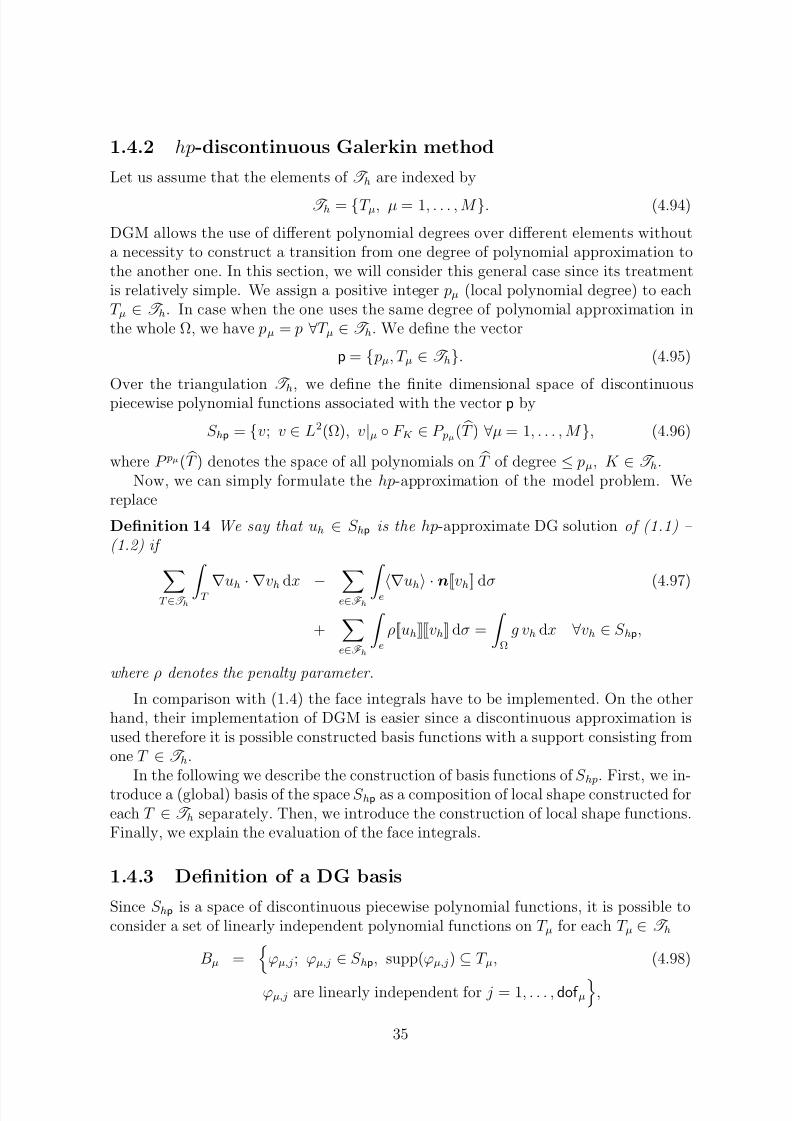
1.4.2 hp-discontinuous Galerkin method
Let us assume that the elements of T h are indexed by
T h = T µ, µ = 1, . . . , M . (4.94)
DGM allows the use of different polynomial degrees over different elements withouta necessity to construct a transition from one degree of polynomial approximation tothe another one. In this section, we will consider this general case since its treatmentis relatively simple. We assign a positive integer pµ (local polynomial degree) to eachT µ ∈ T h. In case when the one uses the same degree of polynomial approximation inthe whole Ω, we have pµ = p ∀T µ ∈ T h. We define the vector
p = pµ, T µ ∈ T h. (4.95)
Over the triangulation T
h, we define the finite dimensional space of discontinuouspiecewise polynomial functions associated with the vector p by
S hp = v; v ∈ L2(Ω), v|µ F K ∈ P pµ( T ) ∀µ = 1, . . . , M , (4.96)
where P pµ( T ) denotes the space of all polynomials on T of degree ≤ pµ, K ∈ T h.Now, we can simply formulate the hp-approximation of the model problem. We
replace
Definition 14 We say that uh ∈ S hp is the hp-approximate DG solution of (1.1) – (1.2) if
T ∈T h T ∇uh · ∇vh dx − e∈F h e∇uh ·n
[[vh]] dσ (4.97)
+e∈F h
e
ρ[[uh]][[vh]] dσ =
Ω
g vh dx ∀vh ∈ S hp,
where ρ denotes the penalty parameter.
In comparison with (1.4) the face integrals have to be implemented. On the otherhand, their implementation of DGM is easier since a discontinuous approximation isused therefore it is possible constructed basis functions with a support consisting fromone T ∈ T h.
In the following we describe the construction of basis functions of S hp. First, we in-troduce a (global) basis of the space S hp as a composition of local shape constructed foreach T ∈ T h separately. Then, we introduce the construction of local shape functions.Finally, we explain the evaluation of the face integrals.
1.4.3 Definition of a DG basis
Since S hp is a space of discontinuous piecewise polynomial functions, it is possible toconsider a set of linearly independent polynomial functions on T µ for each T µ ∈ T h
Bµ =
ϕµ,j; ϕµ,j ∈ S hp, supp(ϕµ,j) ⊆ T µ, (4.98)
ϕµ,j are linearly independent for j = 1, . . . , dof µ,
35
7/23/2019 FEM Implement
http://slidepdf.com/reader/full/fem-implement 36/51
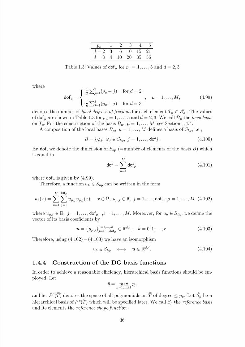
pµ 1 2 3 4 5d = 2 3 6 10 15 21d = 3 4 10 20 35 56
Table 1.3: Values of dof µ for pµ = 1, . . . , 5 and d = 2, 3
where
dof µ =
12
2 j=1( pµ + j) for d = 2
16
3 j=1( pµ + j) for d = 3
, µ = 1, . . . , M , (4.99)
denotes the number of local degrees of freedom for each element T µ ∈ T h. The valuesof dof µ are shown in Table 1.3 for pµ = 1, . . . , 5 and d = 2, 3. We call Bµ the local basis
on T µ. For the construction of the basis Bµ, µ = 1, . . . , M , see Section 1.4.4.A composition of the local bases Bµ, µ = 1, . . . , M defines a basis of S hp, i.e.,
B = ϕ j; ϕ j ∈ S hp, j = 1, . . . , dof . (4.100)
By dof , we denote the dimension of S hp (=number of elements of the basis B) whichis equal to
dof =M µ=1
dof µ. (4.101)
where dof µ is given by (4.99).
Therefore, a function uh ∈ S hp can be written in the form
uh(x) =M µ=1
dof µ j=1
uµ,jϕµ,j(x), x ∈ Ω, uµ,j ∈ R, j = 1, . . . , dof µ, µ = 1, . . . , M (4.102)
where uµ,j ∈ R, j = 1, . . . , dof µ, µ = 1, . . . , M . Moreover, for uh ∈ S hp, we define thevector of its basis coefficients by
u = uµ,jµ=1,...,M j=1,...,dof µ
∈ Rdof , k = 0, 1, . . . , r . (4.103)
Therefore, using (4.102) – (4.103) we have an isomorphism
uh ∈ S hp ←→ u ∈ Rdof . (4.104)
1.4.4 Construction of the DG basis functions
In order to achieve a reasonable efficiency, hierarchical basis functions should be em-ployed. Let
¯ p = maxµ=1,...,M
pµ
and let P ¯ p(
T ) denotes the space of all polynomials on
T of degree ≤ p¯ p. Let S p be a
hierarchical basis of P ¯ p
( T ) which will be specified later. We call ˆS p the reference basis and its elements the reference shape function .
36
7/23/2019 FEM Implement
http://slidepdf.com/reader/full/fem-implement 37/51
Furthermore, let F µ := F T µ , µ = 1, . . . , M , be the mapping introduced by (4.91)
such that F µ(
T ) = T µ. We put
Bµ := ϕµ,j; ϕµ,j(x) = ϕµ,j(F µ(x)) = ϕ j(x), x ∈ T , j = 1, . . . , dof µ, (4.105)
which defines a basis Bµ introduced in (4.98) for each element T µ ∈ T h separately.Finally, (4.100) defines the global basis of S hp.
Reference shape functions
It is possible to use an arbitrary set of (hierarchical or non-hierarchical) shape functionsfor the definition of S p. An example are the Lagrangian and Lobatto shape functionsintroduced in Sections 1.3.1 and 1.3.2, respectively. However, since S hp is the space
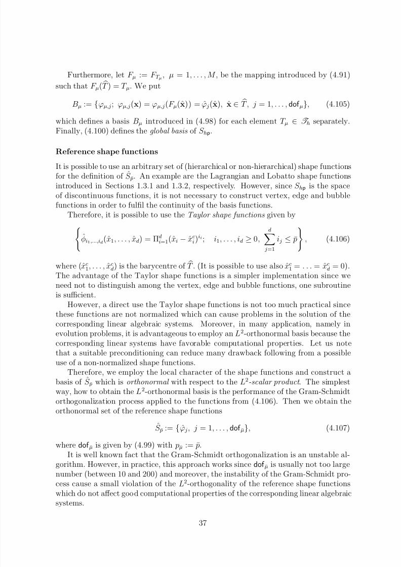
of discontinuous functions, it is not necessary to construct vertex, edge and bubblefunctions in order to fulfil the continuity of the basis functions.Therefore, it is possible to use the Taylor shape functions given by
φi1,...,id(x1, . . . , xd) = Πdi=1(xi − xc
i)ii; i1, . . . , id ≥ 0,
d j=1
i j ≤ ¯ p
, (4.106)
where (xc1, . . . , xc
d) is the barycentre of T . (It is possible to use also xc1 = . . . = xcd = 0).The advantage of the Taylor shape functions is a simpler implementation since weneed not to distinguish among the vertex, edge and bubble functions, one subroutine
is sufficient.However, a direct use the Taylor shape functions is not too much practical sincethese functions are not normalized which can cause problems in the solution of thecorresponding linear algebraic systems. Moreover, in many application, namely inevolution problems, it is advantageous to employ an L2-orthonormal basis because thecorresponding linear systems have favorable computational properties. Let us notethat a suitable preconditioning can reduce many drawback following from a possibleuse of a non-normalized shape functions.
Therefore, we employ the local character of the shape functions and construct abasis of S p which is orthonormal with respect to the L2-scalar product . The simplestway, how to obtain the L2-orthonormal basis is the performance of the Gram-Schmidtorthogonalization process applied to the functions from (4.106). Then we obtain theorthonormal set of the reference shape functions
S p := ϕ j, j = 1, . . . , dof µ, (4.107)
where dof µ is given by (4.99) with pµ := ¯ p.It is well known fact that the Gram-Schmidt orthogonalization is an unstable al-
gorithm. However, in practice, this approach works since dof µ is usually not too largenumber (between 10 and 200) and moreover, the instability of the Gram-Schmidt pro-cess cause a small violation of the L2-orthogonality of the reference shape functions
which do not affect good computational properties of the corresponding linear algebraicsystems.
37
7/23/2019 FEM Implement
http://slidepdf.com/reader/full/fem-implement 38/51
The Gram-Schmidt orthogonalization on the reference element can be carried outsymbolically by some suitable software (e.g., Maple) or numerically. Our numericalexperiments based on the numerical realization of the Gram-Schmidt orthogonalizationwork with success for ¯ p = 10 ⇒ dof µ = 45 (for d = 2).
Let us finally note, the global basis of S hp obtained from (4.100), (4.105) and (4.107)is orthonormal if the mappings F µ := F T µ , µ = 1, . . . , M are linear. Otherwise, someviolations of the L2-orthogonality are presented. However, the mappings F µ, µ =1, . . . , M are close to linear mappings, hence these violations are small and (again) donot affect good computational properties of the corresponding linear algebraic systems.
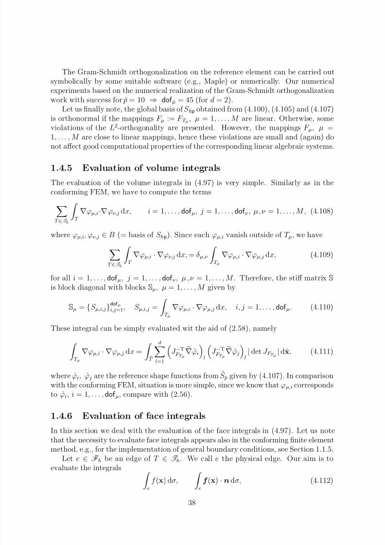
1.4.5 Evaluation of volume integrals
The evaluation of the volume integrals in (4.97) is very simple. Similarly as in the
conforming FEM, we have to compute the termsT ∈T h
T
∇ϕµ,i·∇ϕν,j dx, i = 1, . . . , dof µ, j = 1, . . . , dof ν , µ, ν = 1, . . . , M , (4.108)
where ϕµ,i, ϕν,j ∈ B (= basis of S hp). Since each ϕµ,i vanish outside of T µ, we haveT ∈T h
T
∇ϕµ,i · ∇ϕν,j dx, = δ µ,ν
T µ
∇ϕµ,i · ∇ϕµ,j dx, (4.109)
for all i = 1, . . . , dof µ, j = 1, . . . , dof ν , µ , ν = 1, . . . , M . Therefore, the stiff matrix S
is block diagonal with blocks Sµ, µ = 1, . . . , M given by
Sµ = S µ,i,jdof µi,j=1, S µ,i,j =
T µ
∇ϕµ,i · ∇ϕµ,j dx, i, j = 1, . . . , dof µ. (4.110)
These integral can be simply evaluated wit the aid of (2.58), namely T µ
∇ϕµ,i · ∇ϕµ,j dx =
T
dl=1
J −TF T µ ∇ϕi
l
J −TF T µ ∇ϕ j
l
| det J F T µ | dx, (4.111)
where ϕi, ϕ j are the reference shape functions from S p given by (4.107). In comparison
with the conforming FEM, situation is more simple, since we know that ϕµ,i correspondsto ϕi, i = 1, . . . , dof µ, compare with (2.56).
1.4.6 Evaluation of face integrals
In this section we deal with the evaluation of the face integrals in (4.97). Let us notethat the necessity to evaluate face integrals appears also in the conforming finite elementmethod, e.g., for the implementation of general boundary conditions, see Section 1.1.5.
Let e ∈ F h be an edge of T ∈ T h. We call e the physical edge. Our aim is toevaluate the integrals
ef (x) dσ,
e
f (x) · ndσ, (4.112)
38
7/23/2019 FEM Implement
http://slidepdf.com/reader/full/fem-implement 39/51
where n is the normal vector to e and f : e → R, f : e → R2 are given functions.Let us recall the definition of the face integral. Let ψ = (ψ1, ψ2) : [0, 1] → e be aparameterization of the edge e. Then
e
f (x) dσ =
10
f (ψ(t))
ψ1(t)′
2+
ψ2(t)′2
dt, (4.113)
where ψi(t)′, i = 1, 2 denotes the derivative of ψ1(t) with respect to t.In order to evaluate the integrals (4.112), we use the approach based on the reference
element. Let e be an edge of the reference element T such that T = F T ( T ) ande = F T (e). We call e the reference edge. Let
xe(t) = (xe,1(t), xe,2(t)) : [0, 1] → e (4.114)
be a parameterization of the reference edge e keeping the counterclockwise orientationof the element. Namely, using the notation from Figure 1.6, we have
if T = T t then xe1(t) := (t, 0), t ∈ (0, 1), (4.115)
xe2(t) := (1 − t, t), t ∈ (0, 1),
xe3(t) := (0, 1 − t), t ∈ (0, 1),
if T = T q then xe1(t) := (t, 0), t ∈ (0, 1),
xe2(t) := (1, t), t ∈ (0, 1),
xe3(t) := (1 − t, 1), t ∈ (0, 1),xe4(t) := (0, 1 − t), t ∈ (0, 1).
Moreover, we define the infinitesimal increase of x by
dxe(t) := d
dtxe(t) ∈ R
d, (4.116)
namely
if
T =
T t then dxe1 := (1, 0), t ∈ (0, 1), (4.117)
dxe2 := (−1, 1), t ∈ (0, 1),
dxe3 := (0, −1), t ∈ (0, 1),
if T = T q then dxe1 := (1, 0), t ∈ (0, 1),
dxe2 := (0, 1), t ∈ (0, 1),
dxe3 := (−1, 0), t ∈ (0, 1),
dxe4 := (0, −1), t ∈ (0, 1).
Therefore, the physical edge e is parameterized by
e : x = F T (xe(t)) = (F T,1(xe(t)), F T,2(xe(t))) (4.118)
= (F T,1(xe,1(t), xe,2(t)), F T,2(xe,1(t), xe,2(t))) , t ∈ [0, 1].
39
7/23/2019 FEM Implement
http://slidepdf.com/reader/full/fem-implement 40/51
The first integral from (4.112) is given by
e
f (x) dσ = 10
f (F T (xe(t))) 2i=1
ddt
F T,i(xe(t))1/2
dt (4.119)
=
10
f (F T (xe(t)))
2i,j=1
∂F T,i(xe(t))
∂ x j
d
dtxe,j(t)
1/2
dt
=
10
f (F T (xe(t))) |J F T (xe(t))dxe| dt,
where J F T is the Jacobian matrix of the mapping F T multiplied by the vector dxe (=the infinitesimal increase) and | · | is the Euclid norm of the vector. Let us note that if F T is a linear mapping then e is a straight edge and |J F T (xe(t))dxe(t)| is equal to itslength.
Now, we evaluate the second integral from (4.112). For simplicity, we restrict onlyto the case d = 2. Let re be the tangential vector to e (if e is a straight line thenre = e). Using (4.118) and (4.119), we evaluate re at x(t) = F T (xe(t), t ∈ [0, 1] by
re(x(t)) = (r1(x(t)), r2(x(t))) (4.120)
:= d
dtF T (xe(t)) =
J F T,1(xe(t))dxe, J F T,2(xe(t))dxe
.
Now, be a rotation we obtain the normal vector ne oriented outside of T , namely
ne(x(t)) = (ne,1(x(t)), ne,2(x(t))) : (4.121)
ne,1(x(t)) = re,2(x(t)), ne,2(x(t)) = −re,1(x(t)),
where (te,1, te,2) is the tangential vector to e given by (4.120). Here it is important thatthe counterclockwise orientation of the elements is considered. Therefore, from (4.120)and (4.121), we have
ne(x(t)) = J F T,2(xe(t))dxe, −J F T,1(xe(t))dxe . (4.122)
Let us note that ne(x(t)) is not normalized, it is necessary to divide it by |ne(x(t))| =|J F T (xe(t))dxe|. Finally, similarly as in (4.119), we obtain
e
f (x) · n dσ =
10
f (F T (xe(t))) · ne(x(t))
|ne(x(t))| |J F T (xe(t))dxe| dt, (4.123)
=
10
f (F T (xe(t))) · ne(x(t)) dt,
where ne(x(t)) is given by (4.122). Let us note that if F T is a linear mapping then eis a straight edge and |ne(x(t))| is equal to its length.
40
7/23/2019 FEM Implement
http://slidepdf.com/reader/full/fem-implement 41/51
1.4.7 Data structure
In order to evaluate the integrals (4.111), (4.119) and (4.123), it is enough to evaluate
and store the following data.
(S1) for each T ∈ T h, the determinant of the Jacobi matrix det J F T and the transposedmatrix of the inversion of the Jacobi matrix J TF T ,
(S2) the shape functions ϕi, i = 1, . . . N with the gradients ∇ϕi, i = 1, . . . N on T .
Comparison with the data structures of FEM implementation, we see that (S1) and(S2) are in fact the same but (S3) is missing. This is caused by the fact that we have thedirect connection between the basis functions and the corresponding shape functions,see relation (4.105).
1.5 Numerical quadratures
In the previous sections we assumed that we are able to evaluate all integrals (overthe reference element or the reference edge) exactly. It is true for the model problemwhich is linear and therefore all integrands are polynomial functions. However, when aproblem is nonlinear, it is necessary to use an approximation, namely suitable numer-ical quadratures. Even in case, when the problem is linear, the implementation withnumerical quadratures is more simple.
There exists many numerical quadrature rules with many advantages and disadvan-tages. In the following we exhibits some basis quadrature rules for edge integrals andvolume integrals over the reference square and over the reference triangle, which exhibita reasonable compromise between accuracy and the implementation complexity.
1.5.1 Edge quadratures
We consider the Gauss quadrature rules given by
1
0
f (x) dx ≈ Gk(f ) :=k
i=1
wif (xi), (5.124)
where wi, i = 1, . . . , k and xi, i = 1, . . . , k are the Gauss weights and the Gauss nodes,respectively. Their values can be found in many textbooks, e.g., in [3]. Table 1.4 thesevalues for Gk, k = 1, . . . , 12.
1.5.2 Quadrilaterals quadratures
In order to integrate over the reference square T q, we employ the bi-Gauss quadrature rules given by
T qf (x) dx ≈ G
bik (f ) :=
ki=1
k j=1
wiw jf (xij), (5.125)
41
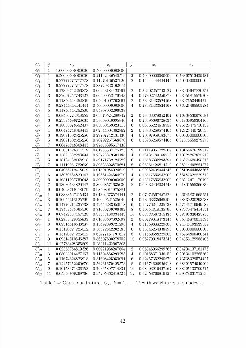
7/23/2019 FEM Implement
http://slidepdf.com/reader/full/fem-implement 42/51
Gk j wj xj j wj xj
G1 1 1.00000000000000 0.50000000000000
G2 1 0.50000000000000 0.21132486540519 2 0.50000000000000 0.78867513459481
G3 1 0.27777777777778 0.11270166537926 2 0.44444444444444 0.50000000000000
G3 3 0.27777777777778 0.88729833462074
G4 1 0.17392742256873 0.06943184420297 2 0.32607257743127 0.33000947820757
G4 3 0.32607257743127 0.66999052179243 4 0.17392742256873 0.93056815579703
G5 1 0.11846344252809 0.04691007703067 2 0.23931433524968 0.23076534494716
G5 3 0.28444444444444 0.50000000000000 4 0.23931433524968 0.76923465505284
G5 5 0.11846344252809 0.95308992296933
G6 1 0.08566224618959 0.03376524289842 2 0.18038078652407 0.16939530676687
G6 3 0.23395696728635 0.38069040695840 4 0.23395696728635 0.61930959304160
G6 5 0.18038078652407 0.83060469323313 6 0.08566224618959 0.96623475710158
G7 1 0.06474248308443 0.02544604382862 2 0.13985269574464 0.12923440720030
G7 3 0.19091502525256 0.29707742431130 4 0.20897959183673 0.50000000000000
G7 5 0.19091502525256 0.70292257568870 6 0.13985269574464 0.87076559279970
G7 7 0.06474248308443 0.97455395617138
G8 1 0.05061426814519 0.01985507175123 2 0.11119051722669 0.10166676129319
G8 3 0.15685332293894 0.23723379504184 4 0.18134189168918 0.40828267875218
G8 5 0.18134189168918 0.59171732124782 6 0.15685332293894 0.76276620495816
G8 7 0.11119051722669 0.89833323870681 8 0.05061426814519 0.98014492824877
G9 1 0.04063719418079 0.01591988024619 2 0.09032408034743 0.08198444633668
G9 3 0.13030534820147 0.19331428364970 4 0.15617353852000 0.33787328829810
G9 5 0.16511967750063 0.50000000000000 6 0.15617353852000 0.66212671170190
G9 7 0.13030534820147 0.80668571635030 8 0.09032408034743 0.91801555366332
G9 9 0.04063719418079 0.98408011975381
G10 1 0.03333567215434 0.01304673574141 2 0.07472567457529 0.06746831665551
G10 3 0.10954318125799 0.16029521585049 4 0.13463335965500 0.28330230293538
G10 5 0.14776211235738 0.42556283050918 6 0.14776211235738 0.57443716949082
G10 7 0.13463335965500 0.71669769706462 8 0.10954318125799 0.83970478414951
G10 9 0.07472567457529 0.93253168334449 10 0.03333567215434 0.98695326425859
G11 1 0.02783428355809 0.01088567092697 2 0.06279018473245 0.05646870011595
G11 3 0.09314510546387 0.13492399721298 4 0.11659688229600 0.24045193539659
G11 5 0.13140227225512 0.36522842202383 6 0.13646254338895 0.50000000000000
G11 7 0.13140227225512 0.63477157797617 8 0.11659688229600 0.75954806460341
G11 9 0.09314510546387 0.86507600278702 10 0.06279018473245 0.94353129988405
G11 11 0.02783428355809 0.98911432907303G12 1 0.02358766819326 0.00921968287664 2 0.05346966299766 0.04794137181476
G12 3 0.08003916427167 0.11504866290285 4 0.10158371336153 0.20634102285669
G12 5 0.11674626826918 0.31608425050091 6 0.12457352290670 0.43738329574427
G12 7 0.12457352290670 0.56261670425573 8 0.11674626826918 0.68391574949909
G12 9 0.10158371336153 0.79365897714331 10 0.08003916427167 0.88495133709715
G12 11 0.05346966299766 0.95205862818524 12 0.02358766819326 0.99078031712336
Table 1.4: Gauss quadratures Gk, k = 1, . . . , 12 with weights wi and nodes xi
42
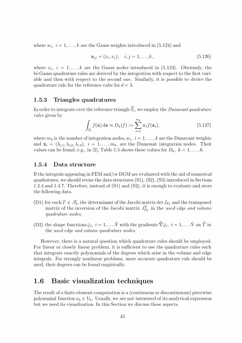
7/23/2019 FEM Implement
http://slidepdf.com/reader/full/fem-implement 43/51
where wi, i = 1, . . . , k are the Gauss weights introduced in (5.124) and
xij = (xi, x j), i, j = 1, . . . , k , (5.126)
where xi, i = 1, . . . , k are the Gauss nodes introduced in (5.124). Obviously, thebi-Gauss quadrature rules are derived by the integration with respect to the first vari-able and then with respect to the second one. Similarly, it is possible to derive thequadrature rule for the reference cube for d = 3.
1.5.3 Triangles quadratures
In order to integrate over the reference triangle
T t, we employ the Dunavant quadrature
rules given by T t
f (x) dx ≈ Dk(f ) :=mki=1
wif (xi), (5.127)
where mk is the number of integration nodes, wi, i = 1, . . . , k are the Dunavant weightsand xi = (λi,1, λi,2, λi,3), i = 1, . . . , mk, are the Dunavant integration nodes. Theirvalues can be found, e.g., in [2], Table 1.5 shows these values for Dk, k = 1, . . . , 6.
1.5.4 Data structure
If the integrals appearing in FEM and/or DGM are evaluated with the aid of numerical
quadratures, we should revise the data structures (S1), (S2), (S3) introduced in Sections1.2.4 and 1.4.7. Therefore, instead of (S1) and (S2), it is enough to evaluate and storethe following data.
(D1) for each T ∈ T h, the determinant of the Jacobi matrix det J F T and the transposedmatrix of the inversion of the Jacobi matrix J TF T in the used edge and volume quadrature nodes ,
(D2) the shape functions ϕi, i = 1, . . . N with the gradients ∇ϕi, i = 1, . . . N on T inthe used edge and volume quadrature nodes .
However, there is a natural question which quadrature rules should be employed.For linear or closely linear problem, it is sufficient to use the quadrature rules suchthat integrate exactly polynomials of the degrees which arise in the volume and edgeintegrals. For strongly nonlinear problems, more accurate quadrature rule should beused, their degrees can be found empirically.
1.6 Basic visualization techniques
The result of a finite element computation is a (continuous or discontinuous) piecewise
polynomial function uh ∈ V h. Usually, we are not interested of its analytical expressionbut we need its visualization. In this Section we discuss these aspects.
43
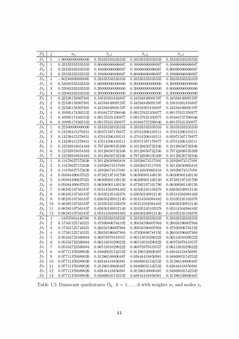
7/23/2019 FEM Implement
http://slidepdf.com/reader/full/fem-implement 44/51
Dk j wj λj,1 λj,2 λj,3
D1 1 1.00000000000000 0.33333333333333 0.33333333333333 0.33333333333333D2 1 0.33333333333333 0.66666666666667 0.16666666666667 0.16666666666667
D2 2 0.33333333333333 0.16666666666667 0.16666666666667 0.66666666666667
D2 3 0.33333333333333 0.16666666666667 0.66666666666667 0.16666666666667
D3 1 -.56250000000000 0.33333333333333 0.33333333333333 0.33333333333333
D3 2 0.52083333333333 0.60000000000000 0.20000000000000 0.20000000000000
D3 3 0.52083333333333 0.20000000000000 0.20000000000000 0.60000000000000
D3 4 0.52083333333333 0.20000000000000 0.60000000000000 0.20000000000000
D4 1 0.22338158967801 0.10810301816807 0.44594849091597 0.44594849091597
D4 2 0.22338158967801 0.44594849091597 0.44594849091597 0.10810301816807
D4 3 0.22338158967801 0.44594849091597 0.10810301816807 0.44594849091597
D4 4 0.10995174365532 0.81684757298046 0.09157621350977 0.09157621350977
D4 5 0.10995174365532 0.09157621350977 0.09157621350977 0.81684757298046
D4 6 0.10995174365532 0.09157621350977 0.81684757298046 0.09157621350977
D5 1 0.22500000000000 0.33333333333333 0.33333333333333 0.33333333333333
D5 2 0.13239415278851 0.05971587178977 0.47014206410511 0.47014206410511
D5 3 0.13239415278851 0.47014206410511 0.47014206410511 0.05971587178977
D5 4 0.13239415278851 0.47014206410511 0.05971587178977 0.47014206410511
D5 5 0.12593918054483 0.79742698535309 0.10128650732346 0.10128650732346
D5 6 0.12593918054483 0.10128650732346 0.10128650732346 0.79742698535309
D5 7 0.12593918054483 0.10128650732346 0.79742698535309 0.10128650732346
D6 1 0.11678627572638 0.50142650965818 0.24928674517091 0.24928674517091
D6 2 0.11678627572638 0.24928674517091 0.24928674517091 0.50142650965818
D6 3 0.11678627572638 0.24928674517091 0.50142650965818 0.24928674517091
D6 4 0.05084490637021 0.87382197101700 0.06308901449150 0.06308901449150
D6 5 0.05084490637021 0.06308901449150 0.06308901449150 0.87382197101700
D6 6 0.05084490637021 0.06308901449150 0.87382197101700 0.06308901449150
D6 7 0.08285107561837 0.05314504984482 0.31035245103378 0.63650249912140
D6 8 0.08285107561837 0.31035245103378 0.63650249912140 0.05314504984482
D6 9 0.08285107561837 0.63650249912140 0.05314504984482 0.31035245103378
D6 10 0.08285107561837 0.31035245103378 0.05314504984482 0.63650249912140
D6 11 0.08285107561837 0.63650249912140 0.31035245103378 0.05314504984482
D6 12 0.08285107561837 0.05314504984482 0.63650249912140 0.31035245103378
D7 1 -.14957004446768 0.33333333333333 0.33333333333333 0.33333333333333
D7 2 0.17561525743321 0.47930806784192 0.26034596607904 0.26034596607904
D7 3 0.17561525743321 0.26034596607904 0.26034596607904 0.47930806784192
D7 4 0.17561525743321 0.26034596607904 0.47930806784192 0.26034596607904
D7 5 0.05334723560884 0.86973979419557 0.06513010290222 0.06513010290222D7 6 0.05334723560884 0.06513010290222 0.06513010290222 0.86973979419557
D7 7 0.05334723560884 0.06513010290222 0.86973979419557 0.06513010290222
D7 8 0.07711376089026 0.04869031542532 0.31286549600487 0.63844418856981
D7 9 0.07711376089026 0.31286549600487 0.63844418856981 0.04869031542532
D7 10 0.07711376089026 0.63844418856981 0.04869031542532 0.31286549600487
D7 11 0.07711376089026 0.31286549600487 0.04869031542532 0.63844418856981
D7 12 0.07711376089026 0.63844418856981 0.31286549600487 0.04869031542532
D7 13 0.07711376089026 0.04869031542532 0.63844418856981 0.31286549600487
Table 1.5: Dunavant quadratures Dk, k = 1, . . . , 6 with weights wi and nodes xi
44
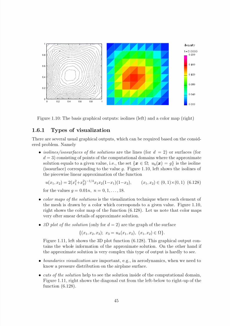
7/23/2019 FEM Implement
http://slidepdf.com/reader/full/fem-implement 45/51
0
0.2
0.4
0.6
0.8
1
0 0.2 0.4 0.6 0.8 1
Figure 1.10: The basis graphical outputs: isolines (left) and a color map (right)
1.6.1 Types of visualization
There are several usual graphical outputs, which can be required based on the consid-ered problem. Namely
• isolines/isosurfaces of the solutions are the lines (for d = 2) or surfaces (ford = 3) consisting of points of the computational domains where the approximatesolution equals to a given value, i.e., the set x ∈ Ω; uh(x) = g is the isoline(isosurface) corresponding to the value g. Figure 1.10, left shows the isolines of the piecewise linear approximation of the function
u(x1, x2) = 2(x21+x2
2)−1/4x1x2(1−x1)(1−x2), (x1, x2) ∈ (0, 1)×(0, 1) (6.128)
for the values g = 0.01n, n = 0, 1, . . . , 18.
• color maps of the solutions is the visualization technique where each element of the mesh is drawn by a color which corresponds to a given value. Figure 1.10,right shows the color map of the function (6.128). Let us note that color mapsvery ofter smear details of approximate solution.
• 3D plot of the solution (only for d = 2) are the graph of the surface
(x1, x2, x3); x3 = uh(x1, x2), (x1, x2) ∈ Ω.
Figure 1.11, left shows the 3D plot function (6.128). This graphical output con-tains the whole information of the approximate solution. On the other hand if the approximate solution is very complex this type of output is hardly to see.
• boundaries visualization are important, e.g., in aerodynamics, when we need toknow a pressure distribution on the airplane surface.
• cuts of the solution help to see the solution inside of the computational domain,Figure 1.11, right shows the diagonal cut from the left-below to right-up of the
function (6.128).
45
7/23/2019 FEM Implement
http://slidepdf.com/reader/full/fem-implement 46/51
0 0.2 0.4 0.6 0.8 1 0
0.20.4
0.60.81
-0.02 0
0.02 0.04 0.06 0.08 0.1
0.12 0.14
0.16
-0.02
0
0.02
0.04
0.06
0.08
0.1
0.12
0.14
0.16
0 0.2 0.4 0.6 0.8 1
Figure 1.11: The basis graphical outputs: a 3D plot (left) and a diagonal cut (right)
1.6.2 Software for visualization
Within this section we briefly describe types of software which can be used for thevisualization of finite element solutions. Our aim is not to give a complete list of allavailable software but give to the readers some overview about possibilities.
We suppose that the software for the visualization can be split into the following
groups.
• Commercial graphical software usually represent a complete tool for visualiza-tion. Let us mention as an example the code Techplot which is able to draw acontinuous piecewise linear or piecewise constant approximate solution for d = 2as well as d = 3 meshes. It allows a wide range of graphical tools, e.g., slices,isosurfaces, cuts, animations etc. However, Techplot uses some postprocessingwhen smooths the given approximate solution. This is advantageous for effectof visualization but it brings some additional perturbation and/or “errors”. Ause of the commercial software does not require any pre-computing, in generally.However, most of the commercial software do not allow a visualization of a higher
order approximation. In this case, some additional technique has to be used, seeSection 1.6.3.
• Free graphical libraries represented, e.g., by PGPLOT, which is a set of Fortran77 subroutines which are able to draw a given line, to fill a given polygon by agive color, etc. Therefore, a use of this library requires a creation of an additionalcode calling the PGPLOT subroutines. This represents an additional work butyou can draw exactly what you want. I.e., no postprocessing perturbs the results.Figure 1.10, right was obtained by PGPLOT.
• Basic graphical code as, e.g., gnuplot are able to carried out basis graphical taskas connecting a given set of nodes. This type of software can be used with
46
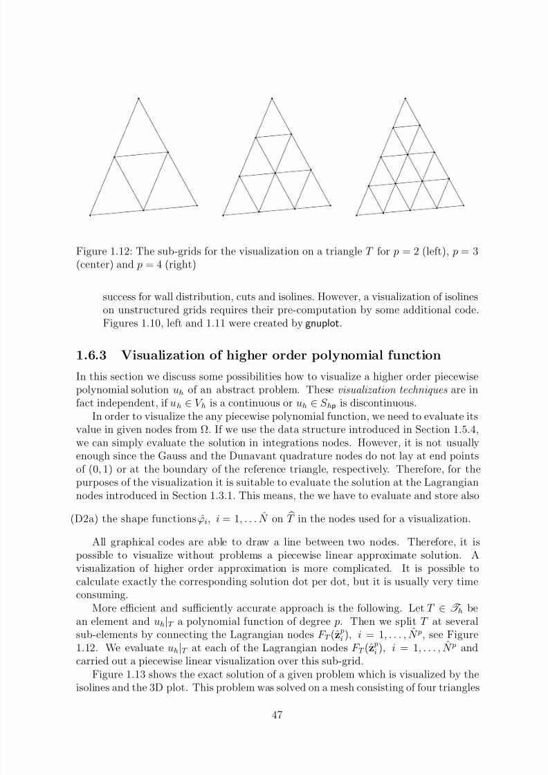
7/23/2019 FEM Implement
http://slidepdf.com/reader/full/fem-implement 47/51
Figure 1.12: The sub-grids for the visualization on a triangle T for p = 2 (left), p = 3(center) and p = 4 (right)
success for wall distribution, cuts and isolines. However, a visualization of isolineson unstructured grids requires their pre-computation by some additional code.Figures 1.10, left and 1.11 were created by gnuplot.
1.6.3 Visualization of higher order polynomial function
In this section we discuss some possibilities how to visualize a higher order piecewisepolynomial solution uh of an abstract problem. These visualization techniques are in
fact independent, if uh ∈ V h is a continuous or uh ∈ S hp is discontinuous.In order to visualize the any piecewise polynomial function, we need to evaluate itsvalue in given nodes from Ω. If we use the data structure introduced in Section 1.5.4,we can simply evaluate the solution in integrations nodes. However, it is not usuallyenough since the Gauss and the Dunavant quadrature nodes do not lay at end pointsof (0, 1) or at the boundary of the reference triangle, respectively. Therefore, for thepurposes of the visualization it is suitable to evaluate the solution at the Lagrangiannodes introduced in Section 1.3.1. This means, the we have to evaluate and store also
(D2a) the shape functions ϕi, i = 1, . . . N on
T in the nodes used for a visualization.
All graphical codes are able to draw a line between two nodes. Therefore, it ispossible to visualize without problems a piecewise linear approximate solution. Avisualization of higher order approximation is more complicated. It is possible tocalculate exactly the corresponding solution dot per dot, but it is usually very timeconsuming.
More efficient and sufficiently accurate approach is the following. Let T ∈ T h bean element and uh|T a polynomial function of degree p. Then we split T at severalsub-elements by connecting the Lagrangian nodes F T (z pi ), i = 1, . . . , N p, see Figure1.12. We evaluate uh|T at each of the Lagrangian nodes F T (z pi ), i = 1, . . . , N p andcarried out a piecewise linear visualization over this sub-grid.
Figure 1.13 shows the exact solution of a given problem which is visualized by theisolines and the 3D plot. This problem was solved on a mesh consisting of four triangles
47
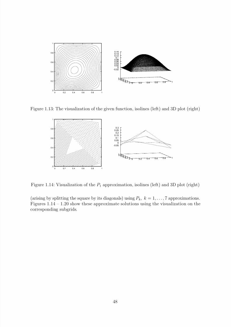
7/23/2019 FEM Implement
http://slidepdf.com/reader/full/fem-implement 48/51
0
0.2
0.4
0.6
0.8
1
0 0.2 0.4 0.6 0.8 1
0 0.2 0.4 0.6 0.8 1 0
0.20.4
0.60.81
-0.02 0
0.02 0.04 0.06 0.08
0.1
0.12 0.14 0.16
Figure 1.13: The visualization of the given function, isolines (left) and 3D plot (right)
0
0.2
0.4
0.6
0.8
1
0 0.2 0.4 0.6 0.8 1
0 0.2 0.4 0.6 0.8 1 0
0.20.4
0.60.81
-0.05
0
0.05
0.1
0.15
0.2
0.25
0.3
Figure 1.14: Visualization of the P 1 approximation, isolines (left) and 3D plot (right)
(arising by splitting the square by its diagonals) using P k, k = 1, . . . , 7 approximations.Figures 1.14 – 1.20 show these approximate solutions using the visualization on thecorresponding subgrids.
48
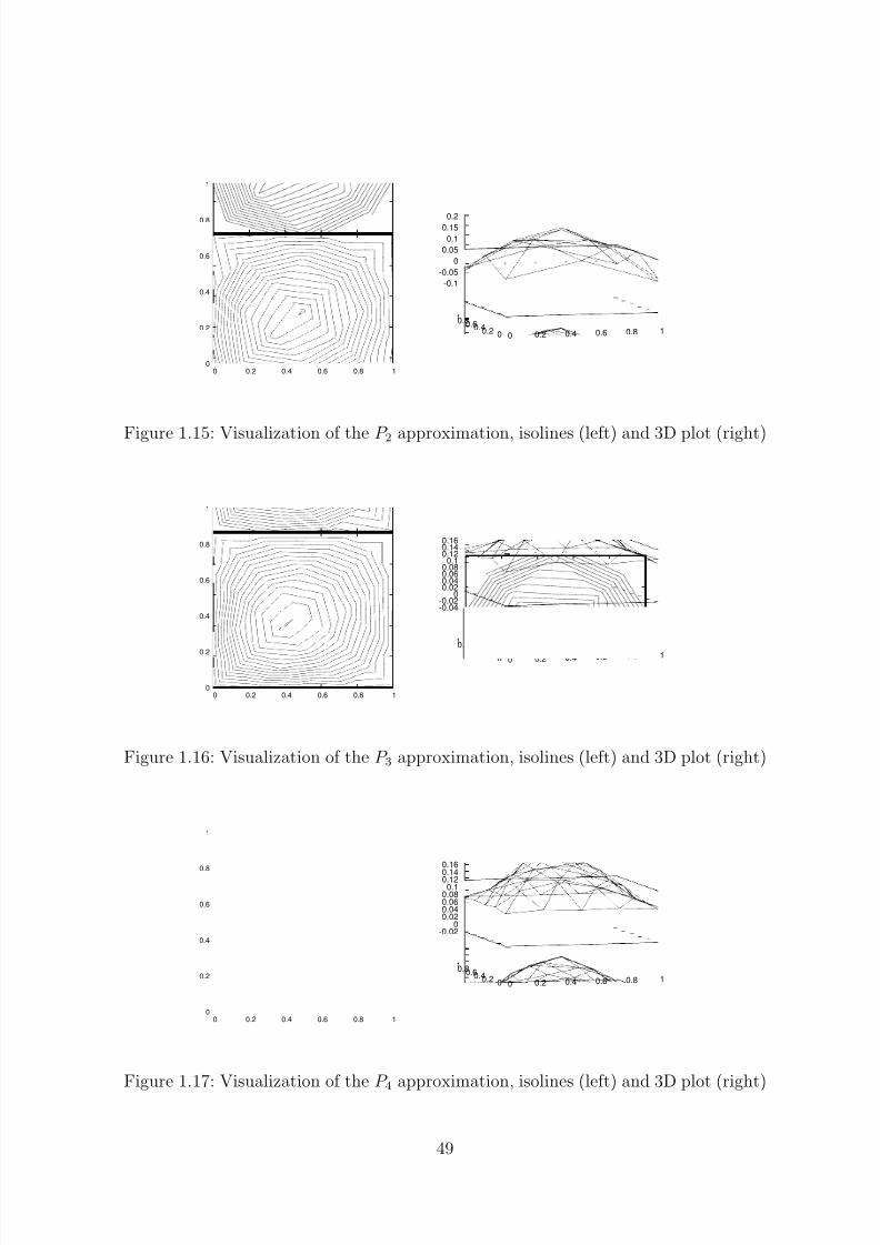
7/23/2019 FEM Implement
http://slidepdf.com/reader/full/fem-implement 49/51
0
0.2
0.4
0.6
0.8
1
0 0.2 0.4 0.6 0.8 1
0 0.2 0.4 0.6 0.8 1 0
0.20.4
0.60.81
-0.1
-0.05
0
0.05
0.1
0.15 0.2
Figure 1.15: Visualization of the P 2 approximation, isolines (left) and 3D plot (right)
0
0.2
0.4
0.6
0.8
1
0 0.2 0.4 0.6 0.8 1
0 0.2 0.4 0.6 0.8 1 00.20.4
0.60.81
-0.04-0.02
0 0.02 0.04 0.06 0.08 0.1
0.12 0.14 0.16
Figure 1.16: Visualization of the P 3 approximation, isolines (left) and 3D plot (right)
0
0.2
0.4
0.6
0.8
1
0 0.2 0.4 0.6 0.8 1
0 0.2 0.4 0.6 0.8 1 0
0.20.4
0.60.81
-0.02 0
0.02 0.04 0.06 0.08 0.1
0.12 0.14
0.16
Figure 1.17: Visualization of the P 4 approximation, isolines (left) and 3D plot (right)
49
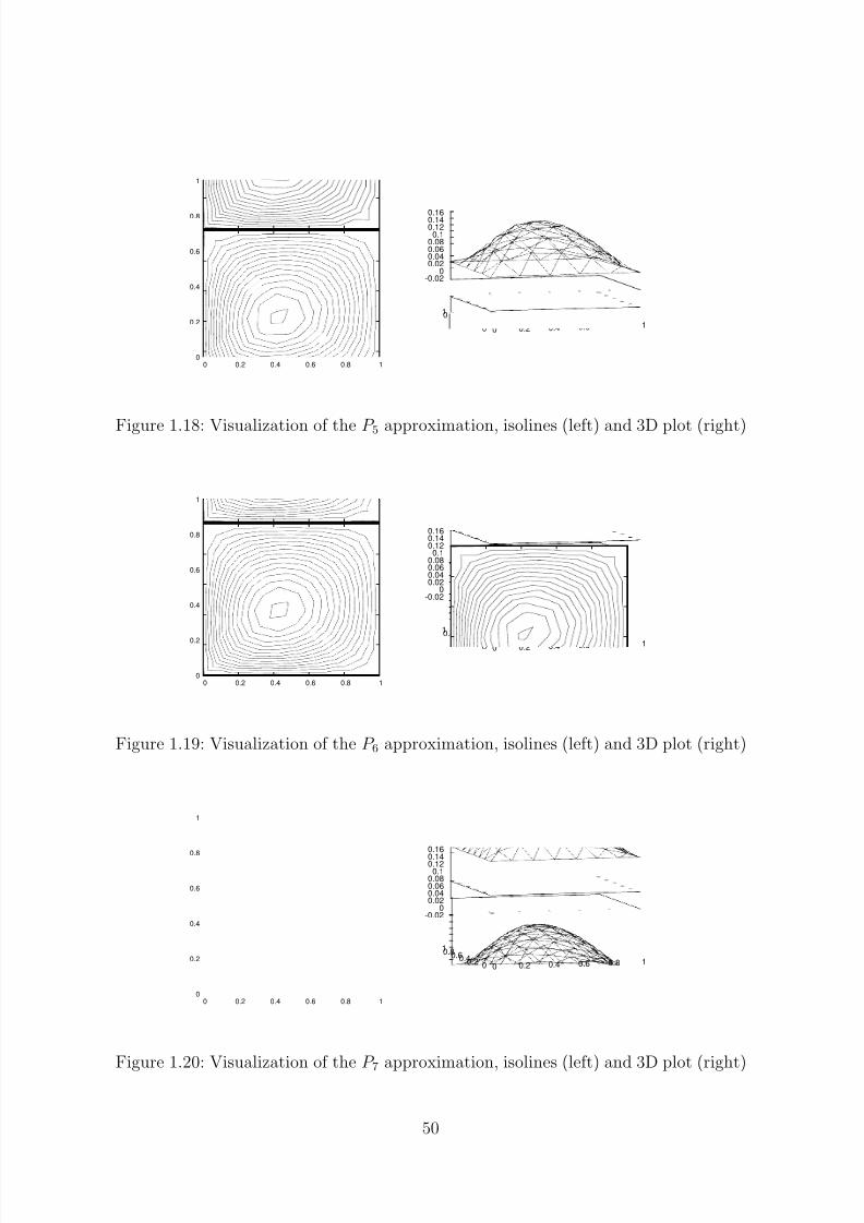
7/23/2019 FEM Implement
http://slidepdf.com/reader/full/fem-implement 50/51
0
0.2
0.4
0.6
0.8
1
0 0.2 0.4 0.6 0.8 1
0 0.2 0.4 0.6 0.8 1 0
0.20.4
0.60.81
-0.02 0
0.02 0.04 0.06 0.08
0.1 0.12 0.14 0.16
Figure 1.18: Visualization of the P 5 approximation, isolines (left) and 3D plot (right)
0
0.2
0.4
0.6
0.8
1
0 0.2 0.4 0.6 0.8 1
0 0.2 0.4 0.6 0.8 1 00.20.4
0.60.81
-0.02 0
0.02 0.04 0.06 0.08
0.1 0.12 0.14 0.16
Figure 1.19: Visualization of the P 6 approximation, isolines (left) and 3D plot (right)
0
0.2
0.4
0.6
0.8
1
0 0.2 0.4 0.6 0.8 1
0 0.2 0.4 0.6 0.8 1 0
0.20.4
0.60.81
-0.02 0
0.02 0.04 0.06 0.08
0.1 0.12 0.14
0.16
Figure 1.20: Visualization of the P 7 approximation, isolines (left) and 3D plot (right)
50
7/23/2019 FEM Implement
http://slidepdf.com/reader/full/fem-implement 51/51
Bibliography
[1] L. Dubcova. hp-FEM for coupled problems in fluid mechanics . PhD thesis, CharlesUniversity Prague, 2010.
[2] D. A. Dunavant. High degree efficient symmetrical gaussian quadrature rules for
the triangle. Int. J. Numer. Methods Eng., 21:1129–1148, 1985.
[3] P. Solın, K. Segeth, and I. Dolezel. Higher-Order Finite Element Methods . Chapman& Hall/CRC Press, 2003.