FEM: Domain Decomposition and Homogenization for Maxwell’s ...
71
FEM: Domain Decomposition and Homogenization for Maxwell’s Equations of Large Scale Problems FEM: Domain Decomposition and Homogenization for Maxwell’s Equations of Large Scale Problems Karl Hollaus Vienna University of Technology, Austria Institute for Analysis and Scientific Computing February 13, 2012
Transcript of FEM: Domain Decomposition and Homogenization for Maxwell’s ...

FEM: Domain Decomposition and Homogenization for Maxwell’s Equations of Large Scale Problems
FEM: Domain Decomposition and Homogenizationfor Maxwell’s Equations of Large Scale Problems
Karl Hollaus
Vienna University of Technology, Austria
Institute for Analysis and Scientific Computing
February 13, 2012

FEM: Domain Decomposition and Homogenization for Maxwell’s Equations of Large Scale Problems
Outline
1 Domain DecompositionIntroductionPoisson Equation
Nitsche-type mortar methodHybride Nitsche-type mortar methodNumerical Examples
Maxwell’s EquationsSteady StateHybride Nitsche-type mortar methodNovel hybride Nitsche-type mortar methodNumerical Examples
2 HomogenizationIntroductionElectrostatic Problem
Two-scale approach
Eddy Current ProblemTwo-scale approach

FEM: Domain Decomposition and Homogenization for Maxwell’s Equations of Large Scale Problems
Domain Decomposition
Introduction
Motivation
Domain Decomposition can be used for:
Moving parts: Electrical machines, etc.Complicated structure: Printed circuit boards, human body,Parallel computingEtc.

FEM: Domain Decomposition and Homogenization for Maxwell’s Equations of Large Scale Problems
Domain Decomposition
Introduction
Problem
Ω ... Domain∂Ω ... Surface of Ω
Ωi ... SubdomainΩ = Ω1 ∪ Ω2
∂Ωi ... Surface of Ωi
Γ ... InterfaceΓ = ∂Ω1 ∩ ∂Ω2

FEM: Domain Decomposition and Homogenization for Maxwell’s Equations of Large Scale Problems
Domain Decomposition
Introduction
Problem
Aim: Non-matching finite element grids and continuoussolutions!
2D:
3D:

FEM: Domain Decomposition and Homogenization for Maxwell’s Equations of Large Scale Problems
Domain Decomposition
Introduction
Electrostatics
Consider the corresponding Maxwell’s equations
curl E = 0
div D = ρ,
the material relation D = ε E and
appropriate boundary conditions.
Then, an electric scalar potential V can be introduced as
E = −∇V
and the Poisson equation
∆V = −ρε
is obtained.

FEM: Domain Decomposition and Homogenization for Maxwell’s Equations of Large Scale Problems
Domain Decomposition
Poisson Equation
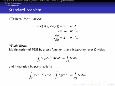
Standard problem
Classical formulation:
−∇(λ(x)∇u(x)) = f in Ω
u = uD on ΓD
λ∂u
∂n= g on ΓN
Weak form:Multiplication of PDE by a test function v and integration over Ω yields∫
Ω
∇(λ∇(u))v dΩ =
∫Ω
fv dΩ,
and integration by parts leads to∫Ω
λ∇u · ∇v dΩ−∫
Γ
λgvn dΓ =
∫Ω
fv dΩ.
FEM: Domain Decomposition and Homogenization for Maxwell’s Equations of Large Scale Problems
Domain Decomposition
Poisson Equation
Standard problem
Classical formulation:
−∇(λ(x)∇u(x)) = f in Ω
u = uD on ΓD
λ∂u
∂n= g on ΓN
Weak form:Multiplication of PDE by a test function v and integration over Ω yields∫
Ω
∇(λ∇(u))v dΩ =
∫Ω
fv dΩ,
and integration by parts leads to∫Ω
λ∇u · ∇v dΩ−∫
Γ
λgvn dΓ =
∫Ω
fv dΩ.

FEM: Domain Decomposition and Homogenization for Maxwell’s Equations of Large Scale Problems
Domain Decomposition
Poisson Equation
Standard problem
Classical formulation:
−∇(λ(x)∇u(x)) = f in Ω
u = uD on ΓD
λ∂u
∂n= 0 on ΓN
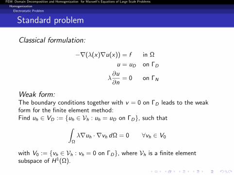
Weak form:The boundary conditions together with v = 0 on ΓD leads to the weakform for the finite element method:Find uh ∈ VD := uh ∈ Vh : uh = uD on ΓD, such that∫
Ω
λ∇uh · ∇vh dΩ =
∫Ω
fvh dΩ ∀vh ∈ V0
with V0 := vh ∈ Vh : vh = 0 on ΓD, where Vh is a finite elementsubspace of H1(Ω).
FEM: Domain Decomposition and Homogenization for Maxwell’s Equations of Large Scale Problems
Domain Decomposition
Poisson Equation
Equivalent transmission problem
Classical formulation:
−∆ui = f in Ωi , i = 1, 2ui = 0 on ∂Ω, i = 1, 2
u1 − u2 = 0 on Γ
∂u1
∂n1+∂u2
∂n2= 0 on Γ,
where ui = u|Ωi .
Definitions:
Jump at the interface: [[u]] := u1n1 + u2n2
Mean value: u := 12 (u1 + u2)

FEM: Domain Decomposition and Homogenization for Maxwell’s Equations of Large Scale Problems
Domain Decomposition
Poisson Equation
Nitsche-type mortar method
Classical formulation:
−∆ui = f in Ωi , i = 1, 2ui = 0 on ∂Ω, i = 1, 2
u1 − u2 = 0 on Γ
∂u1
∂n1+∂u2
∂n2= 0 on Γ,
where ui = u|Ωi .
Idea of Nitsche-type mortar method for domain decomposition:
2∑i=1
∫Ωi
∇u · ∇v dΩ−∫∂Ωi
∇u · [[v ]] ds =
∫Ωi
fv dΩ

FEM: Domain Decomposition and Homogenization for Maxwell’s Equations of Large Scale Problems
Domain Decomposition
Poisson Equation
Nitsche-type mortar method
Weak form:
Find uh ∈ VD := uh ∈ Vh : uh = 0 on ∂Ω, such that
2∑i=1
∫Ωi
∇uh · ∇vh dΩ−∫
Γ
∇uh · [[vh]] ds−∫Γ
∇vh · [[uh]] ds +αp2
h
∫Γ
[[uh]] · [[vh]] ds =
∫Ωi
fvh dΩ ∀vh ∈ V0
with V0 := vh ∈ Vh : vh = 0 on ∂Ω, where Vh is a finite elementsubspace of H1(Ω1)× H1(Ω2).
α ... Stabilization factorp ... Polynomial orderh ... Mesh size

FEM: Domain Decomposition and Homogenization for Maxwell’s Equations of Large Scale Problems
Domain Decomposition
Poisson Equation
Nitsche-type mortar method
Weak form:
Find uh ∈ VD := uh ∈ Vh : uh = 0 on ∂Ω, such that
2∑i=1
∫Ωi
∇uh · ∇vh dΩ−∫
Γ
∇uh · [[vh]] ds−∫Γ
∇vh · [[uh]] ds +αp2
h
∫Γ
[[uh]] · [[vh]] ds =
∫Ωi
fvh dΩ ∀vh ∈ V0
with V0 := vh ∈ Vh : vh = 0 on ∂Ω, where Vh is a finite elementsubspace of H1(Ω1)× H1(Ω2).
The formulation is consistent, stable and bounded w. r. t. a meshdependant energy norm 1.
1Becker, R., P. Hansbo and R. Stenberg, “A finite element method for domaindecomposition with non-matching grids”, 2003

FEM: Domain Decomposition and Homogenization for Maxwell’s Equations of Large Scale Problems
Domain Decomposition
Poisson Equation
Nitsche-type mortar method
Algebraic equation system:
Surface integrals introduce a coupling across the interface Γ:
Ω1︷ ︸︸ ︷ Ω2︷ ︸︸ ︷∗ ∗
∗ ∗
u1
u2
=
f1
f2
The corresponding entries ∗ are almost all zero.
But the integrals of non-zero entries can be difficult to compute!
FEM: Domain Decomposition and Homogenization for Maxwell’s Equations of Large Scale Problems
Domain Decomposition
Poisson Equation
Nitsche-type mortar method
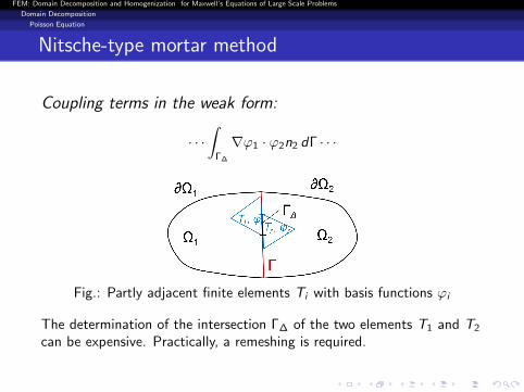
Coupling terms in the weak form:
· · ·∫
Γ∆
∇ϕ1 · ϕ2n2 dΓ · · ·
Fig.: Partly adjacent finite elements Ti with basis functions ϕi
The determination of the intersection Γ∆ of the two elements T1 and T2
can be expensive. Practically, a remeshing is required.

FEM: Domain Decomposition and Homogenization for Maxwell’s Equations of Large Scale Problems
Domain Decomposition
Poisson Equation
Hybride Nitsche-type mortar method
Definition:
Additional independent variable λ, which is the restriction u1 = u2
on Γ
Function space M := µ ∈ L2(∂Ω1 ∪ ∂Ω2) : µ = 0 on ∂Ω

FEM: Domain Decomposition and Homogenization for Maxwell’s Equations of Large Scale Problems
Domain Decomposition
Poisson Equation
Hybride Nitsche-type mortar method
Weak form2:Find (uh, λh) ∈ VD := (uh, λh) ∈ Vh ×Mh : uh = 0 on ∂Ω, such that
2∑i=1
∫Ωi
∇uh·∇vh dΩ−∫∂Ωi
∂uh
∂n(vh − µh) dΓ−
∫∂Ωi
∂vh
∂n(uh − λh) dΓ+
αp2
h
∫∂Ωi
(uh − λh)(vh − µh) dΓ
=
∫Ω
fvh dΩ ∀(vh, µh) ∈ V0
with (uh, λh) ∈ V0 := (vh, µh) ∈ Vh ×Mh : vh = 0 on ∂Ω, where Vh isa finite element subspace of H1(Ω1)× H1(Ω2) and Mh is a subspace ofL2(Γ).
2Egger, H., “A class of hybrid mortar finite element methods for interface problemswith non-matching meshes,” preprint AICES-2009-2, Aachen Institute for AdvancedStudy in Computational Engineering Science, 2009.
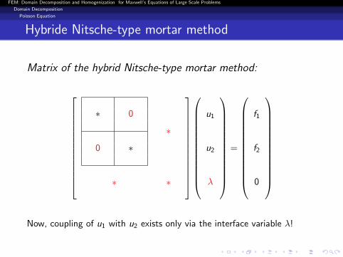
FEM: Domain Decomposition and Homogenization for Maxwell’s Equations of Large Scale Problems
Domain Decomposition
Poisson Equation
Hybride Nitsche-type mortar method
Matrix of the hybrid Nitsche-type mortar method:
∗ 0
0 ∗
∗
∗ ∗
u1
u2
λ
=
f1
f2
0
Now, coupling of u1 with u2 exists only via the interface variable λ!

FEM: Domain Decomposition and Homogenization for Maxwell’s Equations of Large Scale Problems
Domain Decomposition
Poisson Equation
Poisson Equation
We propose a B-spline basis for Mh3:
Mh = S∆ =λ ∈ R | λ|[ti ,ti+1] ∈ Pn , λ ∈ C n−1 ([0, 1])
Gaussian quadrature benefits from smoothness of the splines.
DeBoor recursion
Bi,r (x) =x − ti
ti+r−1 − tiBi,r−1 (x) +
ti+r − x
ti+r − ti+1Bi+1,r−1 (x)
3K. Hollaus, D. Feldengut, J. Schoberl, M. Wabro, D. Omeragic: “Nitsche-typeMortaring for Maxwell’s Equations”’, PIERS Proceedings, 397 - 402, July 5-8,Cambridge, USA 2010.
FEM: Domain Decomposition and Homogenization for Maxwell’s Equations of Large Scale Problems
Domain Decomposition
Poisson Equation
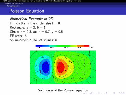
Poisson Equation
Numerical Example in 2D:f = x - 0.7 in the circle, else f = 0Rectangle: a = 2, b = 1Circle: r = 0.3, at: x = 0.7, y = 0.5FE-order: 5Spline-order: 6, no. of splines: 6
Solution u of the Poisson equation
FEM: Domain Decomposition and Homogenization for Maxwell’s Equations of Large Scale Problems
Domain Decomposition
Poisson Equation
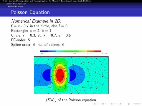
Poisson Equation
Numerical Example in 2D:f = x - 0.7 in the circle, else f = 0Rectangle: a = 2, b = 1Circle: r = 0.3, at: x = 0.7, y = 0.5FE-order: 5Spline-order: 6, no. of splines: 6
(∇u)x of the Poisson equation

FEM: Domain Decomposition and Homogenization for Maxwell’s Equations of Large Scale Problems
Domain Decomposition
Poisson Equation
Poisson Equation
Numerical Example in 3D:f = xz in the cylinder, else f = 0Cuboid: a = 3, b = 2, c = 1Cylinder: r = 0.4, at: x = 1.0, y = 1.0FE-order: 5Spline-order: 6, No. splines: 6
Solution u of the Poisson equation

FEM: Domain Decomposition and Homogenization for Maxwell’s Equations of Large Scale Problems
Domain Decomposition
Poisson Equation
Poisson Equation
Numerical Example in 3D:f = xz in the cylinder, else f = 0Cuboid: a = 3, b = 2, c = 1Cylinder: r = 0.4, at: x = 1.0, y = 1.0FE-order: 5Spline-order: 6, No. splines: 6
(∇u)x of the Poisson equation
FEM: Domain Decomposition and Homogenization for Maxwell’s Equations of Large Scale Problems
Domain Decomposition
Maxwell’s Equations
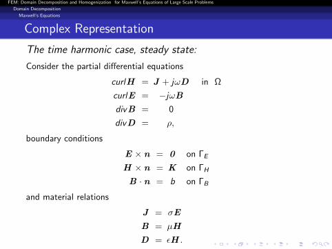
Complex Representation
The time harmonic case, steady state:
Consider the partial differential equations
curlH = J + jωD in Ω
curlE = −jωB
divB = 0
divD = ρ,
boundary conditions
E × n = 0 on ΓE
H × n = K on ΓH
B · n = b on ΓB
and material relations
J = σE
B = µH
D = εH .

FEM: Domain Decomposition and Homogenization for Maxwell’s Equations of Large Scale Problems
Domain Decomposition
Maxwell’s Equations
Standard Problem
Magnetic vector potential A:
A magnetic vector potential A can be introduced as
B = curlA.
Taking acount of the above relations, the physical quantaties can bewritten as
E = −iωA, H = µ−1 curlA
and after known manpulations
curlµ−1 curlA + κA = J in Ω
with the complex conductivity κ = jωσ − ω2ε is obtained.

FEM: Domain Decomposition and Homogenization for Maxwell’s Equations of Large Scale Problems
Domain Decomposition
Maxwell’s Equations
Standard Problem
Classical formulation:
curlµ−1 curlA + κA = J 0 in Ω
µ−1 curlA× n = K on ∂ΩH
A× n = α on ∂ΩB
A× n = 0 on ∂ΩE ,
where ∂Ω = ∂ΩH + ∂ΩB + ∂ΩE .

FEM: Domain Decomposition and Homogenization for Maxwell’s Equations of Large Scale Problems
Domain Decomposition
Maxwell’s Equations
Standard Problem
Weak form:
Considering A× n = 0 on ∂Ω lead to the finite element approximation:Find Ah ∈ VD := Ah ∈ Vh : Ah × n = αh on Ω, such that∫
Ω
µ−1 curlAh curl vh dΩ + jω
∫Ω
κAhvh dΩ =
∫Ω0
J 0vh dΩ
for all vh ∈ V0 := vh ∈ Vh : vh × n = 0 on ∂Ω, where Vh is a finiteelement subspace of H(curl,Ω).

FEM: Domain Decomposition and Homogenization for Maxwell’s Equations of Large Scale Problems
Domain Decomposition
Maxwell’s Equations
Equivalent transmission problem
Classical formulation:
curlµ−1 curlAi + κAi = J 0 in Ωi , i = 1, 2Ai × n = 0 on ∂Ω, i = 1, 2
A1 × n1 + A2 × n2 = 0 on Γ
µ−1 curlA1 × n1 + µ−1 curlA2 × n2 = 0 on Γ,
where Ai = A|Ωi .

FEM: Domain Decomposition and Homogenization for Maxwell’s Equations of Large Scale Problems
Domain Decomposition
Maxwell’s Equations
Hybride Nitsche-type mortar method
Weak form:
Considering homogeneous boundary conditions on ∂Ω and introducingsymmetry, stabilization and hybridization yields the hybrid formulation:
Find (Ah,λ) ∈ VB := Ah ∈ Vh : Ah × n = 0 on ΓB, such that
2∑i=1
∫Ωi
µ−1curlA ·curl v +κA ·v+
∫∂Ωi
µ−1 curlA · [(v − µ)× n]
+
∫∂Ωi
µ−1 curl v · [(A− λ)× n]+αp2
µh
∫∂Ωi
[(A− λ)× n] · [(v − µ)× n]
=
∫Ω
J 0 · v
for all (v ,µ).

FEM: Domain Decomposition and Homogenization for Maxwell’s Equations of Large Scale Problems
Domain Decomposition
Maxwell’s Equations
Novel hybride Nitsche-type mortar method
Novel hybride Nitsche-type mortar method 4:
Considering symmetry, stability and hybridization also for φ leads to
2∑i=1
∫Ωi
µ−1 curlA·curl v+κAv+∫∂Ωi
1
µcurlA [(v−∇ψ−µ)×n]+∫
∂Ωi
1
µcurl v [(A−∇φ− λ)× n]+
α1p2
h
∫∂Ωi
1
µ[(A−∇φ−λ)×n][(v −∇ψ−µ)×n]−
∫∂Ωi
κAn(ψ−ψΓ)−∫∂Ωi
κvn(φ−φΓ)+α2p2
h
∫∂Ωi
κ(φ−φΓ)(ψ−ψΓ)
=
2∑i=1
∫Ωi
J 0v−∫∂Ωi
J nψ
4K. Hollaus, D. Feldengut, J. Schoberl, M. Wabro, D. Omeragic: “Nitsche-typeMortaring for Maxwell’s Equations”’, PIERS Proceedings, 397 - 402, July 5-8,Cambridge, USA 2010.

FEM: Domain Decomposition and Homogenization for Maxwell’s Equations of Large Scale Problems
Domain Decomposition
Maxwell’s Equations
Novel hybride Nitsche-type mortar method
Novel hybride Nitsche-type mortar method:
We propose to descretize by
u, v ... H (curl) conforming finite elements of order p in Ωi
φ, ψ ... H1 conforming finite elements of order p + 1 on ∂Ωi ∩ Γ
φΓ, ψΓ ... tensor product scalar B-splines of order m and
λ, µ ... Nedelec-type B-splines satisfying an exact sequence at Γ

FEM: Domain Decomposition and Homogenization for Maxwell’s Equations of Large Scale Problems
Domain Decomposition
Maxwell’s Equations
Numerical Example
Numerical Example: Permanent MagnetPDE for magnetostatics:
curlµ−1 curl Ai = f (M) in Ωi
A ... Magnetic vector potentialM ... Magnetisation: M 6= 0 in the permanent magnet, else M = 0
Fig.: Two domains (green and blue) with the permanent magnet (red)

FEM: Domain Decomposition and Homogenization for Maxwell’s Equations of Large Scale Problems
Domain Decomposition
Maxwell’s Equations
Numerical Example
Numerical Example: Permanent Magnet
Fig.: Vector plot of the magnetic field intensity H

FEM: Domain Decomposition and Homogenization for Maxwell’s Equations of Large Scale Problems
Domain Decomposition
Maxwell’s Equations
Numerical Example
Numerical Example: Permanent Magnet
Fig.: Scalar plot of the magnetic field intensity Hx

FEM: Domain Decomposition and Homogenization for Maxwell’s Equations of Large Scale Problems
Domain Decomposition
Maxwell’s Equations
Numerical Example
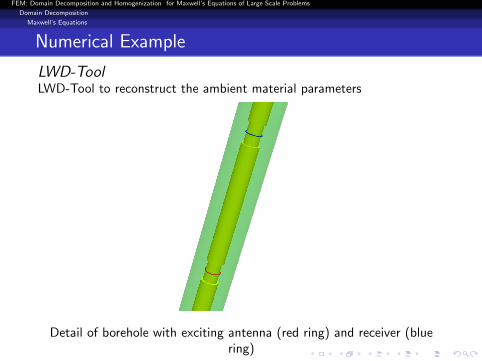
LWD-Tool
LWD ... logging while drilling
Detail of the tool.

FEM: Domain Decomposition and Homogenization for Maxwell’s Equations of Large Scale Problems
Domain Decomposition
Maxwell’s Equations
Numerical Example
LWD-Tool
Ambient soil with a borehole.
FEM: Domain Decomposition and Homogenization for Maxwell’s Equations of Large Scale Problems
Domain Decomposition
Maxwell’s Equations
Numerical Example
LWD-ToolLWD-Tool to reconstruct the ambient material parameters
Detail of borehole with exciting antenna (red ring) and receiver (bluering)
The bore tool is eliminated by surface impedance boundary conditions.

FEM: Domain Decomposition and Homogenization for Maxwell’s Equations of Large Scale Problems
Domain Decomposition
Maxwell’s Equations
Numerical Example
LWD-Tool
Vector plot of the magnetic field intensity H

FEM: Domain Decomposition and Homogenization for Maxwell’s Equations of Large Scale Problems
Domain Decomposition
Maxwell’s Equations
Numerical Example
LWD-Tool
Field lines of the magnetic field intensity H

FEM: Domain Decomposition and Homogenization for Maxwell’s Equations of Large Scale Problems
Domain Decomposition
Maxwell’s Equations
Numerical Example
LWD-Tool
Frequency in kHz Standard: Voltage in µ V NVF: Voltage in µ V20 25.44 -i 18.38 25.43− i 18.37
100 71.68 -i 197.5 71.65− i 197.3400 124.9 -i 963.0 124.9− i 962.3
2000 -634.9 -i 5295 −634.8− i 5290
Table: Numerical results for first order finite elements.
Frequency in kHz Standard: Voltage in µ V NVF: Voltage in µ V20 24.99 -i 18.47 24.98− i 18.47
100 70.25 -i 196.7 70.23− i 196.7400 121.7 -i 957.9 121.7− i 957.7
2000 -648.1 -i 5256 −647.9− i 5255
Table: Numerical results for second order finite elements.
Spline order: 5, spline no.: nϕ = 5, nz = 150

FEM: Domain Decomposition and Homogenization for Maxwell’s Equations of Large Scale Problems
Homogenization
Introduction
Motivation
Laminated transformer core:
Large transformer
Principle of a transformer Laminated transformer core
FEM: Domain Decomposition and Homogenization for Maxwell’s Equations of Large Scale Problems
Homogenization
Introduction
Motivation
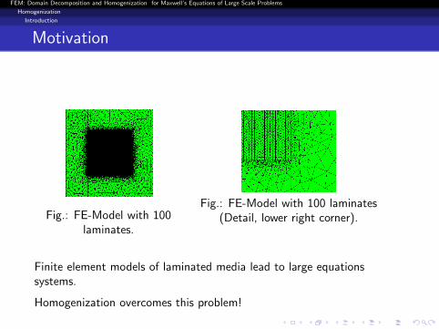
Fig.: FE-Model with 100laminates.
Fig.: FE-Model with 100 laminates(Detail, lower right corner).
Finite element models of laminated media lead to large equationssystems.
Homogenization overcomes this problem!
FEM: Domain Decomposition and Homogenization for Maxwell’s Equations of Large Scale Problems
Homogenization
Introduction
Motivation
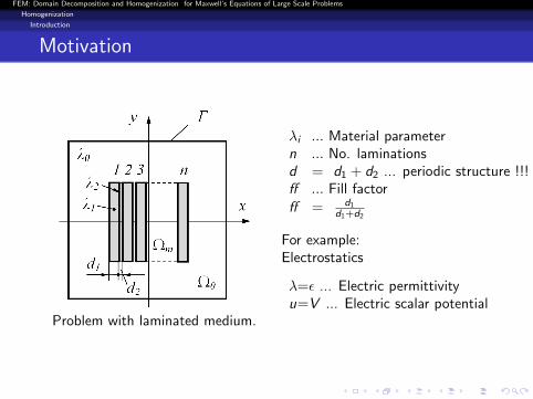
Problem with laminated medium.
λi ... Material parametern ... No. laminationsd = d1 + d2 ... periodic structure !!!ff ... Fill factorff = d1
d1+d2
For example:Electrostatics
λ=ε ... Electric permittivityu=V ... Electric scalar potential
FEM: Domain Decomposition and Homogenization for Maxwell’s Equations of Large Scale Problems
Homogenization
Electrostatic Problem
Electrostatic Problem
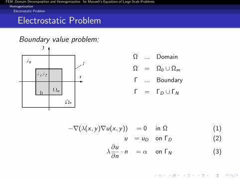
Boundary value problem:
Ω ... Domain
Ω = Ω0 ∪ Ωm
Γ ... Boundary
Γ = ΓD ∪ ΓN
−∇(λ(x , y)∇u(x , y)) = 0 in Ω (1)
u = uD on ΓD (2)
λ∂u
∂n· n = α on ΓN (3)
FEM: Domain Decomposition and Homogenization for Maxwell’s Equations of Large Scale Problems
Homogenization
Electrostatic Problem
Standard problem
Classical formulation:
−∇(λ(x)∇u(x)) = f in Ω
u = uD on ΓD
λ∂u
∂n= 0 on ΓN
Weak form:The boundary conditions together with v = 0 on ΓD leads to the weakform for the finite element method:Find uh ∈ VD := uh ∈ Vh : uh = uD on ΓD, such that∫
Ω
λ∇uh · ∇vh dΩ = 0 ∀vh ∈ V0
with V0 := vh ∈ Vh : vh = 0 on ΓD, where Vh is a finite elementsubspace of H1(Ω).

FEM: Domain Decomposition and Homogenization for Maxwell’s Equations of Large Scale Problems
Homogenization
Electrostatic Problem
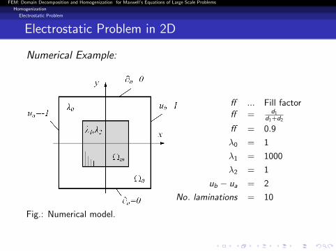
Electrostatic Problem in 2D
Numerical Example:
Fig.: Numerical model.
ff ... Fill factorff = d1
d1+d2
ff = 0.9
λ0 = 1
λ1 = 1000
λ2 = 1
ub − ua = 2
No. laminates = 10

FEM: Domain Decomposition and Homogenization for Maxwell’s Equations of Large Scale Problems
Homogenization
Electrostatic Problem
Electrostatic Problem
Reference solution: Each laminate is modeled individually!
Fig.: Reference solution u of one halfe of the domain.

FEM: Domain Decomposition and Homogenization for Maxwell’s Equations of Large Scale Problems
Homogenization
Electrostatic Problem
Electrostatic Problem
Reference solution:
Solution u, mean value u0 andenvelope u1 along x at y = 0.
Periodic micro-shapefunction φ(x), one periode isshown.

FEM: Domain Decomposition and Homogenization for Maxwell’s Equations of Large Scale Problems
Homogenization
Electrostatic Problem
Electrostatic Problem
Two-scale approach:
Thus, the following approach can be made:
u(x , y) = u0(x , y) + φ(x)u1(x , y)
u0 ... mean valueu1 ... envelope of the staggered partφ ... periodic-micro shape function
Inserting this approach into the bilinear form∫Ω
λ∇u · ∇v dΩ
leads to ∫Ω
λ∇(u0 + φu1) · ∇(v0 + φv1) dΩ = 0.
FEM: Domain Decomposition and Homogenization for Maxwell’s Equations of Large Scale Problems
Homogenization
Electrostatic Problem
Electrostatic Problem
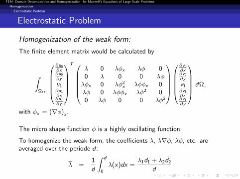
Homogenization of the weak form:
The finite element matrix would be calculated by
∫ΩFE
∂u0
∂x∂u0
∂y
u1∂u1
∂x∂u1
∂y
T
λ 0 λφx λφ 00 λ 0 0 λφλφx 0 λφ2
x λφφx 0λφ 0 λφφx λφ2 00 λφ 0 0 λφ2
∂v0
∂x∂v0
∂y
v1∂v1
∂x∂v1
∂y
dΩ,
with φx = (∇φ)x .
The micro shape function φ is a highly oscillating function.
To homogenize the weak form, the coefficients λ, λ∇φ, λφ, etc. areaveraged over the periode d :
λ =1
d
∫ d
0
λ(x)dx =λ1d1 + λ2d2
d

FEM: Domain Decomposition and Homogenization for Maxwell’s Equations of Large Scale Problems
Homogenization
Electrostatic Problem
Electrostatic Problem
Homogenization of the weak form:
λφx =1
d
∫ d
0
λ(x)φx (x)dx = 2λ1 − λ2
d
λφ =1
d
∫ d
0
λ(x)φ(x)dx = 0
λφ2x =
1
d
∫ d
0
λ(x)φx (x)φx (x)dx =4
d(λ1
d1+λ2
d2)
λφxφ =1
d
∫ d
0
λ(x)φx (x)φ(x)dx = 0
λφ2 =1
d
∫ d
0
λ(x)φ(x)φ(x)dx =λ1d1 + λ2d2
3d
FEM: Domain Decomposition and Homogenization for Maxwell’s Equations of Large Scale Problems
Homogenization
Electrostatic Problem
Electrostatic Problem
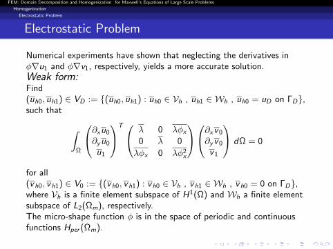
Numerical experiments have shown that neglecting the derivatives inφ∇u1 and φ∇v1, respectively, yields a more accurate solution.Weak form:Find(uh0, uh1) ∈ VD := (uh0, uh1) : uh0 ∈ Vh , uh1 ∈ Wh , uh0 = uD on ΓD,such that
∫Ω
∂x u0
∂y u0
u1
T λ 0 λφx
0 λ 0
λφx 0 λφ2x
∂x v 0
∂y v 0
v 1
dΩ = 0
for all(v h0, v h1) ∈ V0 := (v h0, v h1) : v h0 ∈ Vh , v h1 ∈ Wh , v h0 = 0 on ΓD,where Vh is a finite element subspace of H1(Ω) and Wh a finite elementsubspace of L2(Ωm), respectively.The micro-shape function φ is in the space of periodic and continuousfunctions Hper (Ωm).
FEM: Domain Decomposition and Homogenization for Maxwell’s Equations of Large Scale Problems
Homogenization
Electrostatic Problem
Electrostatic Problem in 2D
Numerical Example:
Fig.: Numerical model.
ff ... Fill factorff = d1
d1+d2
ff = 0.9
λ0 = 1
λ1 = 1000
λ2 = 1
ub − ua = 2
No. laminations = 10

FEM: Domain Decomposition and Homogenization for Maxwell’s Equations of Large Scale Problems
Homogenization
Electrostatic Problem
Electrostatic Problem
Comparison of the results:
Fig.: Reference solution. Fig.: Homogenized solution.
The agreement between reference solution and homogenized solution isobviously excellent!

FEM: Domain Decomposition and Homogenization for Maxwell’s Equations of Large Scale Problems
Homogenization
Electrostatic Problem
Electrostatic Problem
Comparison of the results: flux density λ (∇φ)x
Fig.: Reference solution. Fig.: Homogenized solution.

FEM: Domain Decomposition and Homogenization for Maxwell’s Equations of Large Scale Problems
Homogenization
Electrostatic Problem
Eddy Current Problem in 2D
Boundary value problem:
Ω ... DomainΩ = Ω0 ∪ Ωm
Γ ... Boundary
Γ = ΓH ∪ ΓB
µ ... Magnetic permeability
σ ... Electric conductivity
J 0 ... Impressed current density in a coil
B ... Magnetic flux density
Assumptions:- Linear material properties
- Time harmonic case, steady
state
FEM: Domain Decomposition and Homogenization for Maxwell’s Equations of Large Scale Problems
Homogenization
Eddy Current Problem
Eddy Current Problem
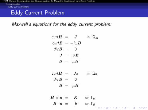
Maxwell’s equations for the eddy current problem:
curlH = J in Ωm
curlE = −jωB
divB = 0
J = σE
B = µH
curlH = J 0 in Ω0
divB = 0
B = µH
H × n = K on ΓH
B · n = b on ΓB
FEM: Domain Decomposition and Homogenization for Maxwell’s Equations of Large Scale Problems
Homogenization
Eddy Current Problem
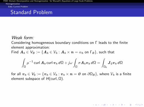
Standard Problem
Weak form:Considering homogeneous boundary conditions on Γ leads to the finiteelement approximation:Find Ah ∈ VB := Ah ∈ Vh : Ah × n = αh on ΓB, such that∫
Ω
µ−1 curlAh curl vh dΩ + jω
∫Ω
σAhvh dΩ =
∫Ω0
J 0vh dΩ
for all vh ∈ V0 := vh ∈ Vh : vh × n = 0 on ∂ΩB, where Vh is a finiteelement subspace of H(curl,Ω).
FEM: Domain Decomposition and Homogenization for Maxwell’s Equations of Large Scale Problems
Homogenization
Eddy Current Problem
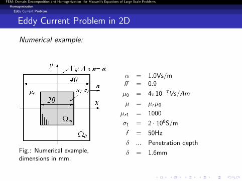
Eddy Current Problem in 2D
Numerical example:
Fig.: Numerical example,dimensions in mm.
α = 1.0Vs/mff = 0.9
µ0 = 4π10−7Vs/Am
µ = µrµ0
µr1 = 1000
σ1 = 2 · 106S/m
f = 50Hz
δ ... Penetration depth
δ = 1.6mm

FEM: Domain Decomposition and Homogenization for Maxwell’s Equations of Large Scale Problems
Homogenization
Eddy Current Problem
Eddy Current Problem
Reference solution:
Eddy currents in laminates, 2D problem
Two-scale approach:
A = A0 + φ(0,A1)T +∇(φw)
A0 ... represents the mean value of the solution
φ(0,A1)T considers J y and
w∇(φw) models J x at the end of the laminates.

FEM: Domain Decomposition and Homogenization for Maxwell’s Equations of Large Scale Problems
Homogenization
Eddy Current Problem
Eddy Current Problem
Homogenized weak form:
Inserting the approach into the bilinear form yields:∫Ω
µ−1curl(A0 + φ(0,A1)T +∇(φw)
)curl
(v0 + φ(0, v1)T +∇(φq)
)dΩ
+jω
∫Ω
σ(A0 + φ(0,A1)T +∇(φw)
) (v0 + φ(0, v1)T +∇(φq)
)dΩ =
∫Ω0
J 0v dΩ
(4)

FEM: Domain Decomposition and Homogenization for Maxwell’s Equations of Large Scale Problems
Homogenization
Eddy Current Problem
Eddy Current Problem
Finite element stiffness matrix:
Bilinearform: ∫Ω
µ−1curlA · curlv dΩ
Homogenized finite element matrix:∫ΩFE
(curlA0
A1
)T (ν νφx
νφx νφ2x
)(curlv0
v1
)dΩ,
with the reluctivity ν = µ−1.
FEM: Domain Decomposition and Homogenization for Maxwell’s Equations of Large Scale Problems
Homogenization
Eddy Current Problem
Eddy Current Problem
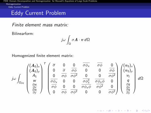
Finite element mass matrix:
Bilinearform:
jω
∫Ω
σA · v dΩ
Homogenized finite element matrix:
jω
∫ΩFE
(A0)x
(A0)y
A1
w∂w∂x∂w∂y
T
σ 0 0 σφx σφ 00 σ σφ 0 0 σφ
0 σφ σφ2 0 0 σφ2
σφx 0 0 σφ2x σφxφ 0
σφ 0 0 σφxφ σφ2 0
0 σφ σφ2 0 0 σφ2
(v0)x
(v0)y
v1
q∂q∂x∂q∂y
dΩ

FEM: Domain Decomposition and Homogenization for Maxwell’s Equations of Large Scale Problems
Homogenization
Eddy Current Problem
Eddy Current Problem
Homogenized weak form:Find (A0h,A1h,w h) ∈ VB := (A0h , A1h , w h) : A0h ∈ Uh , A1h ∈Vh , w h ∈ Wh and A0h × n = αh on ΓB, such that
A(A0h,A1h; v0h, v 1h) + B(A0h,A1h,w h; v0h, v 1h, qh) = f (v0h) (5)
for all (v0h, v 1h, qh) ∈ V0 := (v0h , v 1h , qh) : v0h ∈ Uh, v 1h ∈Vh , qh ∈ Wh and v0h × n = 0 on ΓB, where Uh is a finite elementsubspace of H(curl,Ω), Vh a finite element subspace of L2(Ωm) and Wh
a finite element subspace of H1(Ωm), respectively.The micro-shape function φ is in the space of periodic and continuousfunctions Hper (Ωm).
Again, a coarse finite element mesh suffices for the homogenized medium!

FEM: Domain Decomposition and Homogenization for Maxwell’s Equations of Large Scale Problems
Homogenization
Eddy Current Problem
Eddy Current Problem in 2D
Numerical example:
Fig.: Numerical example,dimensions in mm.
α = 1.0Vs/mff = 0.9
µ0 = 4π10−7Vs/Am
µ = µrµ0
µr1 = 1000
σ1 = 2 · 106S/m
f = 50Hz
δ ... Penetration depth
δ = 1.6mm

FEM: Domain Decomposition and Homogenization for Maxwell’s Equations of Large Scale Problems
Homogenization
Eddy Current Problem
Eddy Current Problem
Comparison of the results: Eddy current density J
Reference solution. Homogenized solution.
... solution in the upper left corner: d1 = 1.8mm, 10 laminations
The agreement between reference solution and homogenized solution isobviously excellent!
FEM: Domain Decomposition and Homogenization for Maxwell’s Equations of Large Scale Problems
Homogenization
Eddy Current Problem
Eddy Current Problem
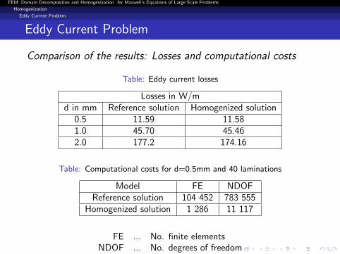
Comparison of the results: Losses and computational costs
Table: Eddy current losses
Losses in W/md in mm Reference solution Homogenized solution
0.5 11.59 11.581.0 45.70 45.462.0 177.2 174.16
Table: Computational costs for d=0.5mm and 40 laminations
Model FE NDOFReference solution 104 452 783 555
Homogenized solution 1 286 11 117
FE ... No. finite elementsNDOF ... No. degrees of freedom

FEM: Domain Decomposition and Homogenization for Maxwell’s Equations of Large Scale Problems
Homogenization
Eddy Current Problem
Thank you for your attention!


![A BLOCH DECOMPOSITION–BASED SPLIT-STEP … · Finally, the use of the Bloch transformation in problems of homogenization has been discussed in [12, 14] and numerically studied in](https://static.fdocuments.net/doc/165x107/5e5d536b9c04af49a04d4642/a-bloch-decompositionabased-split-step-finally-the-use-of-the-bloch-transformation.jpg)