FEM ANALYSIS OF THE CYCLIC BEHAVIOUR OF STEEL BEAMTO ...
95
FEM ANALYSIS OF THE CYCLIC BEHAVIOUR OF STEEL BEAMTO- COLUMN JOINTS Hafiz Muhammad Ubaid Ur Rehman February, 2018 Thesis submitted in partial fulfilment of the requirements for SUSCOS_M European Master in Sustainable Constructions under natural hazards and catastrophic events, and supervised by Professor Doctor Luis Alberto Proença Simoes da Silva and Assistant Professor Ricardo Joel Teixeira Costa
Transcript of FEM ANALYSIS OF THE CYCLIC BEHAVIOUR OF STEEL BEAMTO ...

FEM ANALYSIS OF THE CYCLICBEHAVIOUR OF STEEL BEAMTO-
COLUMN JOINTS
Hafiz Muhammad Ubaid Ur Rehman
February, 2018
Thesis submitted in partial fulfilment of the requirements for SUSCOS_MEuropean Master in Sustainable Constructions under natural hazards andcatastrophic events , and supervised by Professor Doctor Luis AlbertoProença Simoes da Silva and Assistant Professor Ricardo Joel Teixeira Costa


FEM ANALYSIS OF THE CYCLIC BEHAVIOUR OF STEEL BEAM-
TO-COLUMN JOINTS
Author: Hafiz Muhammad Ubaid Ur Rehman, Civil, Engr.
Supervisor: Prof. Luis Alberto Proenca Simoes da Silva, PhD
Asst. Prof. Ricardo Joel Teixeira Costa, PhD
University: University of Coimbra, Coimbra, Portugal
University of Coimbra, Coimbra, Portugal February, 2018


European Erasmus Mundus Master
Sustainable Constructions under natural hazards and catastrophic events
520121-1-2011-1-CZ-ERA MUNDUS-EMMC
FEM ANALYSIS OF THE CYCLIC BEHAVIOUR OF STEEL BEAM-
TO-COLUMN JOINTS
Hafiz Muhammad Ubaid Ur Rehman February, 2018


European Erasmus Mundus Master
Sustainable Constructions under natural hazards and catastrophic events
520121-1-2011-1-CZ-ERA MUNDUS-EMMC
Members of the Jury
President: Prof. Aldina Maria da Cruz Santiago, PhD
Department of Civil Engineering - FCTUC Rua Luís Reis Santos - Pole II of the University 3030 - 788 Coimbra, Portugal
Thesis Supervisor:
Prof. Luis Alberto Proenca Simoes da Silva, PhD
Department of Civil Engineering - FCTUC Rua Luís Reis Santos - Pole II of the University 3030 - 788 Coimbra, Portugal
Members:
Prof. Carlos Alberto da Silva Rebelo, PhD
Department of Civil Engineering - FCTUC Rua Luís Reis Santos - Pole II of the University 3030 - 788 Coimbra, Portugal
Prof. Ricardo Joel Teixeira Costa, PhD
Department of Civil Engineering - FCTUC Rua Luís Reis Santos - Pole II of the University 3030 - 788 Coimbra, Portugal


European Erasmus Mundus Master
Sustainable Constructions under natural hazards and catastrophic events
520121-1-2011-1-CZ-ERA MUNDUS-EMMC
i
ACKNOWLEDGMENT
Thanks ALLAH ALMIGHTY for taking care of me at every step of my life.
The success and final outcome of this project required a lot of guidance and assistance for many
people and I am extremely privilege to have got this all along the completion of my dissertation.
All that I have done is only due to such supervision and assistance and I would not forget to thank
them.
I respect and thank Prof. Luis Alberto Proenca Simoes da Silva, for providing me an opportunity
to do the project work within the framework of RFCS project EQUALJOINTS in Institute of
Sustainability and Innovation in Structural Engineering (ISISE), University of Coimbra and
guiding me, all support and guidance which made me complete the project duly. I am extremely
thankful to him for providing such a nice support and direction, although he had busy schedule
managing the departmental activities.
I owe my deep gratitude as well to my project co-supervisor Asst. Prof. Ricardo Joel Teixeira
Costa, who took keen interest on my project work and guided me all along, till the completion of
my project work by providing all the necessary information for developing a good model.
I would not forget to remember Asst. Prof. Helder David Craveiro of Institute of Sustainability
and Innovation in Structural Engineering (ISISE), University of Coimbra for his encouragement
and more over for his timely support and guidance till the completion of my project work.
I heartily thank my parents, family members and friends who help me a lot in finalizing this project
within the limited time frame.


European Erasmus Mundus Master
Sustainable Constructions under natural hazards and catastrophic events
520121-1-2011-1-CZ-ERA MUNDUS-EMMC
ii
ABSTRACT
The construction of a structure undergoes several stages, each of which must be thoroughly
thought. In structures that may be subject to seismic actions at some point of their use life, these
considerations are especially significant. Joints between steel elements in this type of structures
should always be designed, fabricated and erected such that brittle failure is avoided and a ductile
mode of failure governs the collapse.
Designers must always bear in mind design requirements set by the relevant design standards. In
Europe, EN1993 must be observed for the seismic design of structures, with significant reference
to EN1993 for the design of steel structures and EN1993-1-8 in particular for the design of steel
joints making use of the components method.
Nowadays the experimental test is the preferred method between the scientific community to
assess the seismic behavior of steel joints. However, the analysis of the seismic behavior of beam-
to-columns joints at component level directly from the analysis of the results of the experimental
test is unfeasible. Accordingly, advanced numerical models must be developed and validated with
the experimental tests.
In this dissertation advanced FEM based models are developed for the analysis of monotonic
and cyclic behavior of the tension region of beam-to-column steel joints in the framework of the
project “European pre-qualified steel joints (EQUALJOINTS)”, focusing in the behavior of the
column flange in bending.


European Erasmus Mundus Master
Sustainable Constructions under natural hazards and catastrophic events
520121-1-2011-1-CZ-ERA MUNDUS-EMMC
iii
NOTATION
General
tf Flange or plate thickness
leff Total effective length of an equivalent T-stub
F Force
FT, I, Rd Design resistance for each T-stub mode
Mpl, Rd Resistance of the formed plastic hinges
Ft, Rd Bolt’s tension resistance
m Bolt distance to the weld
n Minimum bolt distance to a free edge
fy Yield strength
fu Ultimate strength
fub Bolt ultimate strength
As Tensile area of a bolt
k2 Bolt strength reduction factor
K Stiffness
E Elastic modulus
Et Tangent modulus

European Erasmus Mundus Master
Sustainable Constructions under natural hazards and catastrophic events
520121-1-2011-1-CZ-ERA MUNDUS-EMMC
iv
Eu Ultimate modulus
Q Prying force
Greek letters
𝛾𝛾𝑀𝑀𝑀𝑀 Partial safety factor used for applied design situations
Ϭtrue True stress
Ϭengg. Engineering stress
Ɛ true True strain
Ɛ engg. Engineering strain
Ɛ pl Plastic strain
Acronyms
MISES Von Mises stresses
PEEQ Equivalent plastic strain

European Erasmus Mundus Master
Sustainable Constructions under natural hazards and catastrophic events
520121-1-2011-1-CZ-ERA MUNDUS-EMMC
v
Table of Contents ACKNOWLEDGMENT -------------------------------------------------------------------------------------- i
ABSTRACT---------------------------------------------------------------------------------------------------- ii
NOTATION --------------------------------------------------------------------------------------------------- iii
List of Figures ------------------------------------------------------------------------------------------------ vii
List of Tables--------------------------------------------------------------------------------------------------- x
1. Introduction ------------------------------------------------------------------------------------------------- 1
1.1 Background --------------------------------------------------------------------------------------------- 1
1.2. Motivation ---------------------------------------------------------------------------------------------- 2
1.3. Main goals and scope --------------------------------------------------------------------------------- 3
2. State of Art -------------------------------------------------------------------------------------------------- 4
2.1. Behaviour of Joints Under Seismic Load ---------------------------------------------------------- 4
2.2. Experimental Program on Bolted T-stub under Cyclic Loads ---------------------------------- 7
2.3. The Component Method ---------------------------------------------------------------------------- 11
2.3.1. The T-Stub model ------------------------------------------------------------------------------ 15
3. Finite Element Modeling (FEM) ------------------------------------------------------------------------ 22
3.1. FEM elements in ABAQUS ------------------------------------------------------------------------ 22
3.1.1. Family ----------------------------------------------------------------------------------------------- 22
3.1.2. Degrees of freedom -------------------------------------------------------------------------------- 23
3.1.3. Number of nodes (Order of interpolation) ----------------------------------------------------- 23
3.1.4. Formulation ----------------------------------------------------------------------------------------- 24
3.1.5. Integration ------------------------------------------------------------------------------------------ 25
3.2. Solid Elements ---------------------------------------------------------------------------------------- 25
3.2.1. Choosing between quadrilateral and tetrahedral mesh element shapes ----------------- 26
3.2.2. Choosing between first-order and second-order elements -------------------------------- 26
3.3. Material Model in FEM ----------------------------------------------------------------------------- 26
3.4. Constrain and Contact Interaction ----------------------------------------------------------------- 28

European Erasmus Mundus Master
Sustainable Constructions under natural hazards and catastrophic events
520121-1-2011-1-CZ-ERA MUNDUS-EMMC
vi
3.5. Loading ------------------------------------------------------------------------------------------------ 30
4. Numerical Model ------------------------------------------------------------------------------------------ 31
4.1. Simplified Model Geometry and Boundaries ---------------------------------------------------- 31
4.2. Parametric Analysis---------------------------------------------------------------------------------- 32
4.3. FEM Model Construction --------------------------------------------------------------------------- 33
4.3.1. Part Module -------------------------------------------------------------------------------------- 33
4.3.2. Property Module -------------------------------------------------------------------------------- 34
4.3.3. Assembly Module ------------------------------------------------------------------------------ 35
4.3.4. Step Module ------------------------------------------------------------------------------------- 35
4.3.5. Interaction Module ----------------------------------------------------------------------------- 36
4.3.6. Load Module ------------------------------------------------------------------------------------ 37
4.3.7. Mesh Module ------------------------------------------------------------------------------------ 38
4.3.8. Visualization Module -------------------------------------------------------------------------- 39
4.2. Loading Protocol ------------------------------------------------------------------------------------- 40
5. Results and Discussion ----------------------------------------------------------------------------------- 43
5.1. FEM Models Definition ----------------------------------------------------------------------------- 43
5.2. Monotonic Behaviour ------------------------------------------------------------------------------- 49
5.2.3. Column Flange in Bending -------------------------------------------------------------------- 49
5.2.4. Overall Model ----------------------------------------------------------------------------------- 55
5.3. Cyclic Behaviour ------------------------------------------------------------------------------------- 58
5.3.1. Column Flange in Bending -------------------------------------------------------------------- 58
5.3.2. Overall Model ----------------------------------------------------------------------------------- 66
6. Conclusions and Recommendations for Future works ----------------------------------------------- 70
6.1. Conclusions ------------------------------------------------------------------------------------------- 70
6.2. Recommendations for Future works -------------------------------------------------------------- 71
7. References -------------------------------------------------------------------------------------------------- 72

European Erasmus Mundus Master
Sustainable Constructions under natural hazards and catastrophic events
520121-1-2011-1-CZ-ERA MUNDUS-EMMC
vii
List of Figures
Figure 2.1: Results of monotonic tests [8] ...................................................................................... 7
Figure 2.2: Failure mode of specimen under cyclic tests [8] .......................................................... 8
Figure 2.3: Specimen´s behaviour belonging to A series [8] .......................................................... 9
Figure 2.4: Specimen´s behaviour belonging to series C [8] ........................................................ 10
Figure 2.5: Typical beam-to-column end-plate bolted joint [11] ................................................. 12
Figure 2.6: Design moment-rotation characteristics for a joint [2] .............................................. 13
Figure 2.7: T-Stub Geometry ........................................................................................................ 15
Figure 2.8: Failure mode 1 (ductile mode) ................................................................................... 16
Figure 2.9: Failure mode 2 (Intermediate mode) ......................................................................... 16
Figure 2.10: Failure mode 3 (brittle mode) ................................................................................... 16
Figure 2.11: Schematic failure modes of T-Stub [13] .................................................................. 17
Figure 2.12: Ductile failure mode & Intermediate failure mode in T-Stub profiles [14 ] ............ 17
Figure 2.13: Dimensions of an equivalent T-stub flange [13] ...................................................... 18
Figure 2.14: Type of failure depending on the geometry of T-Stub [2] ....................................... 19
Figure 2.15: Values of α for stiffened column flanges and end-plates [2] ................................... 21
Figure 3.1: Element families in ABAQUS software [16] ............................................................ 23
Figure 3.2: Linear brick, quadratic brick, and modified tetrahedral element [16] ........................ 23
Figure 3.3: Naming convention of solid elements in ABAQUS [16] ........................................... 25
Figure 3.4: Stress vs strain ............................................................................................................ 28
Figure 3.5: Bolts pre-loading plane [11] ....................................................................................... 30
Figure 4.1: Tension part of beam-to-column joint ........................................................................ 31
Figure 4.2: 3D view of the tension region of the beam-column joint ........................................... 32
Figure 4.3: Geometrical description of the components ............................................................... 34
Figure 4.4: Description of assembly module of a model. ............................................................ 35
Figure 4.5: Description of interaction module of a model. ........................................................... 37

European Erasmus Mundus Master
Sustainable Constructions under natural hazards and catastrophic events
520121-1-2011-1-CZ-ERA MUNDUS-EMMC
viii
Figure 4.6: Description of load module of a model. ..................................................................... 38
Figure 4.7: FEM mesh of the parts of the model, a) end plate, b) HEA 300, c) beam flange, d) bolt, and e) stiffener ...................................................................................................................... 39
Figure 4.8: Von Misses stresses and equivalent plastic strains visualization in visualization module of ABAQUS. ................................................................................................................................. 40
Figure 4.9: Force displacement curve in visualization module of ABAQUS............................. 40
Figure 4.10: Loading protocol for a T-stub [3] ............................................................................. 42
Figure 5.1: Predefine nodes to assess the deformation of column flange in bending [11] ........... 50
Figure 5.2: Force-Deformation curve and bilinear approximation for the column flange in bending in model 1 ..................................................................................................................................... 51
Figure 5.3: Force-Deformation curve and bilinear approximation for the column flange in bending in model 2 ..................................................................................................................................... 51
Figure 5.4: Force-Deformation curve and bilinear approximation for the column flange in bending in model 3 ..................................................................................................................................... 52
Figure 5.5: Force-Deformation curve and bilinear approximation for the column flange in bending in model 4 ..................................................................................................................................... 52
Figure 5.6: Force-Deformation curves for the column flange in bending .................................... 53
Figure 5.7: Normalized Force-Deformation curves for monotonically loaded models ................ 54
Figure 5.8: Force-Displacement curves for monotonically loaded model of joints ..................... 55
Figure 5.9: Normalized Force-Displacement curves for monotonically loaded model of joints .. 56
Figure 5.10:Von Mises stress for monotonically loaded models .................................................. 57
Figure 5.11: Force-Deformation curves for the column flange in bending under cyclic and monotonic loads – model 1. .......................................................................................................... 58
Figure 5.12: Force-Deformation curves for the column flange of Model 2 under cyclic and monotonic loads ............................................................................................................................ 59
Figure 5.13: Force-Deformation curves for the column flange of Model 3 under cyclic and monotonic loads ............................................................................................................................ 59
Figure 5.14: Force-Deformation curves for the column flange of Model 4 under cyclic and monotonic loads ............................................................................................................................ 60
Figure 5.15: Force-Deformation curves for the column flange of All Models under cyclic loads61
Figure 5.16: Normalized Force-Displacement curves for cyclic loaded models .......................... 62

European Erasmus Mundus Master
Sustainable Constructions under natural hazards and catastrophic events
520121-1-2011-1-CZ-ERA MUNDUS-EMMC
ix
Figure 5.17: Energy dissipation in the column flange in bending. ............................................... 63
Figure 5.18: Accumulative energy dissipation in the column flange in bending. ........................ 64
Figure 5.19: Normalized energy dissipation for the column flange in bending ........................... 65
Figure 5.20: Accumulative normalized energy dissipation for the column flange in bending ..... 65
Figure 5.21: Force-Displacement curves for cyclic loaded models .............................................. 66
Figure 5.22: Normalized Force-Displacement curves for cyclic loaded models ......................... 67
Figure 5.23: Energy dissipation by entire joint models. ............................................................... 68
Figure 5.24: Accumulative energy dissipation by entire joint models. ........................................ 69


European Erasmus Mundus Master
Sustainable Constructions under natural hazards and catastrophic events
520121-1-2011-1-CZ-ERA MUNDUS-EMMC
x
List of Tables
Table 2.1: Dissipation capacity of single joint component [7] ....................................................... 5
Table 2.2: List of components [2] ................................................................................................. 14
Table 2.3: Effective length of end plate [2] .................................................................................. 20
Table 2.4: Effective length for stiffened column flange [2] ......................................................... 20
Table 3.1: Elastic properties of material ....................................................................................... 26
Table 3.2: Plastic properties of material for mild steel ................................................................. 27
Table 3.3: Plastic properties of material for bolts. ........................................................................ 27
Table 4.1: Description of the procedures used to draw the parts of the model. ............................ 33
Table 4.2: Material assigned to the parts of the model ................................................................. 34
Table 4.3: Simplified loading protocol [3] ................................................................................... 41
Table 4 4: Loading protocol for the T-stub [3] ............................................................................. 42
Table 5.1: Effective length for a stiffened column flange in a bolted connection. ....................... 43
Table 5.2: Strength of column flange in bending - model 1. ........................................................ 44
Table 5.3: Strength of column flange in bending - model 2. ........................................................ 44
Table 5.4: Strength of column flange in bending - model 3. ........................................................ 45
Table 5.5: Strength of column flange in bending - model 4. ........................................................ 45
Table 5.6: Effective length for end plate in a bolted connection .................................................. 46
Table 5.7: Strength of beam end plate - model 1. ......................................................................... 47
Table 5.8: Strength of beam end plate - model 2. ......................................................................... 47
Table 5.9: Strength of beam end plate - model 3. ......................................................................... 48
Table 5.10: Strength of beam end plate - model 4. ....................................................................... 48
Table 5.11: Comparison of T-stub response obtained from EC3-1-3 and numerical models ...... 53
Table 5.12: Energy dissipation for the column flange in bending (J). .......................................... 63
Table 5.13: Normalized energy dissipation for the column flange in bending ............................ 64

European Erasmus Mundus Master
Sustainable Constructions under natural hazards and catastrophic events
520121-1-2011-1-CZ-ERA MUNDUS-EMMC
xi
Table 5.14: Energy dissipation for the entire joint model (J). ..................................................... 68

European Erasmus Mundus Master
Sustainable Constructions under natural hazards and catastrophic events
520121-1-2011-1-CZ-ERA MUNDUS-EMMC
1
1. Introduction
1.1 Background
As in all types of structures, the cyclic behavior of beam-to-column steel joints may have a major
influence on the performance of moment resisting frames during an earthquake.
However, the analysis and design of steel buildings according to EN 1993-1 [1] and EN 1993-1 [2]
may be based on centerline frame models – where the geometry and the mechanical properties of the
beam-to-column steel joints is not explicitly modeled – when the beam-to-column joints are full-
strength and rigid thus enforcing the formation of dissipative zones near the ends of the beam members
[3].
On the other hand, in case of partial strength and/or semi-rigid beam-to-column steel joints, EN 1993-
1 [2] allows beam-to-column joints to be the dissipative zones itself. In this case: (i) the joints must
have rotation capacity higher than the rotation demands, (ii) the adjacent members framing into the
joints must have a stable behavior at ultimate limit conditions and (iii) the effect of the joint
deformation on global behavior must be taken into account in the global analysis of structure through
a non-linear static (pushover) analysis or non-linear response-history analysis. In this case, refined
models, accounting for the beam-to-column joint cyclic behavior, are required for the analysis and
design of the structures [3].
EN 1993-1-8 [2] provides a procedure based in the so-called component method to assess the strength
and stiffness of beam-to-column joints. However, it does not provide tools to assess neither the rotation
capacity nor the cyclic behavior of these structural elements [3].
This work is in the scope of the research project “European pre-qualified steel joints
(EQUALJOINTS) Grant agreement no. RFSR-CT-2013-00021” carried out Institute for
Sustainability and Innovation in Structural Engineering (ISISE) in University of Coimbra,
Coimbra, Portugal.
European Erasmus Mundus Master
Sustainable Constructions under natural hazards and catastrophic events
520121-1-2011-1-CZ-ERA MUNDUS-EMMC
2
1.2. Motivation
In order to achieve a good seismic performance of moment resisting frames (MRFs) with reduced
costs, these structures are designed to concentrate the dissipation of the energy induced by
earthquakes in specific zones so called dissipative zones. In particular, the design of steel moment
resisting frames according to EC8, can be carried out by locating the dissipative zones in beams
or joints [4]. The location of dissipative zones can be controlled by capacity design according to a
strength hierarchy criterion.
In particular, when full strength joints are adopted, joints are designed to be over strength with
respect to the connected members and, therefore, the plastic hinges are located at beam ends by
means of cyclic inelastic bending, so that dynamic inelastic analyses require the modelling of the
cyclic response of the beams where plastic hinges develop. This approach can lead, in some
structural situations such as the case of structures with few storeys and/ or with long spans where
the design of beams is mainly governed by vertical loads rather than the lateral ones, to column
sections significantly greater than those strictly necessary to withstand the member loads [5,6].
On the other hand, partial strength joints can be employed in order to concentrate the plastic zones
in the connections. Aforementioned approach is allowed by EC3 [2] which clearly states that the
plastic hinges can be developed at the end of the beam or in the joint. In these cases, the response
of the joints in term of stiffness, resistance and ductility is a key aspect for design purposes. An
analytical procedure to predict the response of joints based on knowledge of mechanical and
geometrical properties of individual element of the joint (the components), subjected to static
loading condition are available and is known as the “component method”. In order to extend the
component approach to the prediction of the seismic response of partial strength joints, the
modelling of the cyclic response of the joint components is necessary.
In case of bolted connections, the main joint components responsible for the joint ductility, such
as the column flange in bending, the end-plate in bending and the angles in tension may be modeled
by means of a simplified model known as “T-Stub” [2].

European Erasmus Mundus Master
Sustainable Constructions under natural hazards and catastrophic events
520121-1-2011-1-CZ-ERA MUNDUS-EMMC
3
1.3. Main goals and scope
The main goal of this dissertation is the development of advanced Finite Element Models to assess
the cyclic behaviour of column flanges in bending of beam-to-column end plate bolted
connections. Having into account the complex behaviour of full beam-to-column joints, partial
models were used to allow to assess accurately the internal forces and the deformation of the
column flange in bending. The models and the load history was define based in the testes and in
the findings of EQUALJOINTS project. More in particular, the goal of this dissertation is to assess
the influence of the collapse mode of the column flange in bending on its cyclic behaviour. The T-
stub model was used as starting point to define the parametric analysis.

European Erasmus Mundus Master
Sustainable Constructions under natural hazards and catastrophic events
520121-1-2011-1-CZ-ERA MUNDUS-EMMC
4
2. State of Art
2.1. Behaviour of Joints Under Seismic Load
In MRFs, the seismic resistance of structure should be provided based in a strength hierarchy
among members and joints. According to the capacity design concept, such a structure will be able
to dissipate part of the energy induced by the ground motion through plastic deformations in the
dissipative zones of ductile members, e.g. through bending deformation in beams of Moment
Resisting Frames (MRF) – formation of plastic hinges in columns is prevented to avoid the
premature collapse of the structure [2] and to allow the mobilization of a large number of
dissipative zones by the collapse mechanism. Accordingly, the region where dissipative zones will
appear in beams or joints is set by means of an appropriate choice of the ratio between the flexural
resistance of the beams and the bending resistance of the joint.
If the dissipative regions are in the beams ends, joints have to be full strength and take into account
the possible over strength effects, which leads to expensive joints solutions.
On the other hand, the use of partial strength joint is permitted but the number of requirements to
be respected for this joint typology is such that it is currently essential to accomplish experimental
tests to check when these requirements are satisfied. The component method is a solution to
overcome the “full strength” limitation. This method considers any joint as a set of individual basic
component [2] and computes the behaviour of the joint from the behaviour of these basic
components.
The probability of forecasting the behaviour of beam to column joints under cyclic loading
conditions allows the design of structures able to dissipate the earthquake input energy by means
of a stable hysteretic behaviour of beam end and/or of their joints to the columns.
It is necessary to preliminarily analyse the dissipation capacity of the beam to column joint
components that are affected by seismic actions. Accordingly, it is recommended to distinguish
between dissipative and non-dissipative components, i.e., dissipative and non-dissipative failure

European Erasmus Mundus Master
Sustainable Constructions under natural hazards and catastrophic events
520121-1-2011-1-CZ-ERA MUNDUS-EMMC
5
mechanisms [7]. With reference to joint components this distinction can be made according to
Table 2.1.
Table 2.1: Dissipation capacity of single joint component [7]
Component Dissipative Non-Dissipative 1 Column web panel in shear ✔
2 Column web in compression 2.1 without buckling ✔ 2.2 with buckling ✔
3 Column web in tension ✔
4 Column flange in bending 4.1 welded joints ✔ 4.2 bolted joints ✔
5 End plate in bending ✔
6 Flange cleat in bending 6.1 without local buckling ✔ 6.2 premature local buckling ✔
7 Beam web in tension ✔ 8 Plate in tension ✔
9 Plate in compression 9.1 without local buckling ✔ 9.2 premature local buckling ✔
10 Bolt in tension ✔ 11 Bolt in shear ✔
12 Bolt in bearing ( on beam flange, column flange, end plate or cleat) ✔
The knowledge of the joint cyclic response and its modelling represents an essential point when
the frame design is based on the dissipation of the seismic input energy in the linking elements.
Many research programs have been carried out worldwide on the cyclic response of beam to
column joints to identify the behaviour parameters governing the cyclic response and at the
modeling of hysteretic behaviour. Furthermore, many efforts have carried to identify low cycle
fatigue [8].

European Erasmus Mundus Master
Sustainable Constructions under natural hazards and catastrophic events
520121-1-2011-1-CZ-ERA MUNDUS-EMMC
6
Mostly research works deals with the whole joint response and its modelling. This methodology
does not permit an easy identification of the contribution of each component and, as a result, of
the role played by the geometrical and mechanical parameters. A different methodology can be
based on the statement that the cyclic behaviour of beam-to-column joints can be predicted by
properly combining the cyclic response of its basic components. This methodology represents the
extension to the cyclic behaviour of the component approach widely investigated in the case of
monotonic loading conditions [8].
The components governing the cyclic response of partially restrained bolted connections have been
identified so that the idea of predicting the cyclic response of connections starting from the
knowledge of the cyclic response of their basic components has given impetus for research, both
experimental analysis and modelling, on isolated joint components [4,5,6,9]. In particular,
Swanson and Leon [9] have tested 48 isolated T-stubs with the primary goal of developing design
rules for T-stub joints that would result in a full strength joint, ductile behaviour and a joint
stiffness close to the full restraint range. In addition, they tested also six full scale beam to column
joints indicating that the T-stubs in the full scale tests performed very similarly to those tested as
components.
An accurate forecast of the joint rotational performance under cyclic loads, relied on the
component methodology, involves the preliminary characterization of the cyclic response of the
joint components. For this reason, following dissertation dedicated to the analysis of the cyclic
behaviour of the most important component of bolted joints, i.e. bolted T-stubs. In this work,
analytical results are resumed and the preliminary models for predicting the cyclic response of
such fundamental components are presented and discussed.

European Erasmus Mundus Master
Sustainable Constructions under natural hazards and catastrophic events
520121-1-2011-1-CZ-ERA MUNDUS-EMMC
7
2.2. Experimental Program on Bolted T-stub under Cyclic Loads
In [8], author investigated cyclic response of T-stub under cyclic loading conditions and monotonic
loading conditions on the basis of experimental tests on T- stub assemblages. In that research,
author examined 28 specimens, 20 under cyclic loading conditions with constant amplitude, 4
under cyclic loading conditions with variable amplitude and 4 under monotonic loading conditions.
From 28 specimens, 7 derived from a HEA 180 profile (series HEA 180), from a HEB 180 profile
(series HEB 180), 7 composed by welding with flange thickness equal to 12 mm (series W12) and
7 composed by welding with flange thickness equal to 18 mm (series W18). 1 monotonic test, 5
constant amplitude test, 1 variable amplitude test had been carried out with reference to each series
of specimens.
The main objective of the monotonic tests was the investigation of plastic deformation capacity of
the specimens whose values had been adopted for development of the range of the amplitude
values to be used in cyclic tests. The results of all monotonic tests are presented in Figure 2.1.
Figure 2.1: Results of monotonic tests [8]

European Erasmus Mundus Master
Sustainable Constructions under natural hazards and catastrophic events
520121-1-2011-1-CZ-ERA MUNDUS-EMMC
8
With respect to cyclic tests, author [8] found that all specimens belonging to HEA 180 and W12
series, showed same failure mode independent of the imposed displacement amplitude. Initially
formation of cracks in flanges is in the central part of flange at the flange to web connection zone
the number of cycles corresponding to the development of first cracking was dependent on the
displacement amplitude of the cyclic test, being as much greater as smaller is the displacement.
These cracks progressively propagated toward the flange edges up to the complete fracture of one
flange which causes the complete loss of load carrying capacity by increasing the number of the
cycles, shown in Figure 2.2.
Figure 2.2: Failure mode of specimen under cyclic tests [8]
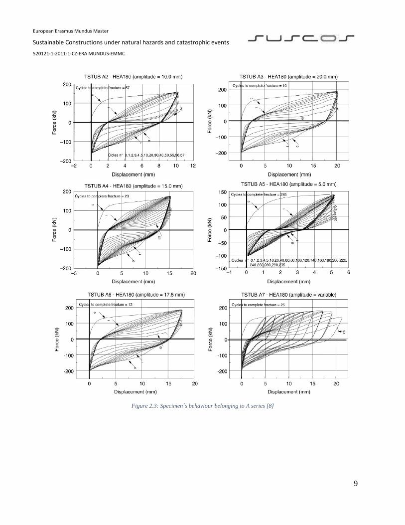
This type of behaviour leads to a progressive deterioration, up to failure, of axial strength, stiffness
and energy dissipation capacity, as presented in Figure 2.3 and in Figure 2.4. Author [8] concluded
that all aforementioned specimens showed different collapse mechanism under monotonic loading
conditions and under cyclic loading conditions, where the yielding of flanges were accompanied
by the bolt fracture. On the other hand, specimens belonging to HEB 180 and W 18 series, the
cyclic behaviour was characterized by horizontal slips before reloading due to relevant plastic
deformations of the bolts. During these slips the axial force is equal to zero up to the recovery of
the bolt plastic deformation before reloading. While this type of premature failure mode was not
observed in HEA 180 and W 12 series, subjected to cyclic loading.
European Erasmus Mundus Master
Sustainable Constructions under natural hazards and catastrophic events
520121-1-2011-1-CZ-ERA MUNDUS-EMMC
9
Figure 2.3: Specimen´s behaviour belonging to A series [8]

European Erasmus Mundus Master
Sustainable Constructions under natural hazards and catastrophic events
520121-1-2011-1-CZ-ERA MUNDUS-EMMC
10
Figure 2.4: Specimen´s behaviour belonging to series C [8]

European Erasmus Mundus Master
Sustainable Constructions under natural hazards and catastrophic events
520121-1-2011-1-CZ-ERA MUNDUS-EMMC
11
The stiffness and degradation laws had been proposed both in case of specimens failing, under
monotonic loads, according to type 1 and in the case of specimens failing, under monotonic loads,
according to either type 2 or type 3 failure mode by [8].
In addition, his work also proposed that, as the failure mode under monotonic loading conditions
can be different from that occurring under cyclic loads, the correlation between the energy
dissipation corresponding to the failure condition and the energy dissipated in monotonic
conditions up to a displacement amplitude equal to that of the cyclic tests have been provided.
On the basis of the above analysis, semi-analytical models for predicting the cyclic behaviour of
the T-stub assemblages starting from their geometrical and mechanical properties have been
developed. Finally, the degree of accuracy of the proposed models have been pointed out by the
good agreement with the experimental results in terms of energy dissipation capacity [8].
2.3. The Component Method
The component method has the prospective to predict the response of joints, whatever geometrical
configuration of joint and type of member cross sections, under any loading condition (axial
loading, bending or cyclic loading etc.) but for that, it is required to know the exact behaviour of
each component shown in Table 2.2, see Figure 2.5. To know the behaviour of the joint it is
essential to know post yield behaviour of components accounting for strain hardening effects, their
ultimate resistance, their deformations ability but also the degradation of their strength and
stiffness, due to cyclic loads [10].
The following steps are required for application of the component method:
1. Identification:
Active component of concern joint should be identifying;
2. Characterization:
Evaluation of the behaviour of each individual component;

European Erasmus Mundus Master
Sustainable Constructions under natural hazards and catastrophic events
520121-1-2011-1-CZ-ERA MUNDUS-EMMC
12
3. Assembly:
Assembly of all constituent components and evaluation of the behaviour of the
entire beam-to-column joint.
The strength of basic components in tension or compression is usually based on an effective width
(beff) while the strength of a basic component under bending or subjected to transverse forces is
based on equivalent T-Stub, i.e. a geometrical idealization of T profile made of a web in tension
and a flange in bending bolted by the flange [10].
Figure 2.5: Typical beam-to-column end-plate bolted joint [11]
The component method allows to determine the bending moment resistance (M j, Rd), the rotational
stiffness (S j) and the rotation capacity (ϕ Cd), according to the scheme of Figure 2.6. The design
moment resistance (M j, Rd) is equal to the maximum moment of design moment-rotation curve,
and is defined by Eq. 2.1
𝑀𝑀𝑗𝑗,𝑅𝑅𝑅𝑅 = ∑ ℎ𝑟𝑟𝐹𝐹𝑡𝑡𝑟𝑟,𝑅𝑅𝑅𝑅𝑟𝑟 Eq. 2.1
where Ftr, Rd is the effective design tension resistance of bolt-row r, hr is the distance from bolt row
r to the centre of compression and r is the bolt-row number. If the bolt-rows in tension are more

European Erasmus Mundus Master
Sustainable Constructions under natural hazards and catastrophic events
520121-1-2011-1-CZ-ERA MUNDUS-EMMC
13
than one, then they are numbered starting from the bolt-row farthest from the centre of
compression. The rotational stiffness (S j) is a secant stiffness, moment require to produce unit
rotation in a joint. For a design moment-rotation characteristic this definition of Sj applies up to
the rotation ϕxd at which Mj, Ed first reaches Mj, Rd, but not for larger rotations as shown in Figure
2.6. The initial Sj, ini. which is slope of elastic range of the design moment-rotation characteristic.
Sj is defined by Eq. 2.2
𝑆𝑆𝑗𝑗 = 𝐸𝐸𝐸𝐸2
𝜇𝜇 ∑ 1𝑘𝑘𝑖𝑖𝑖𝑖
Eq. 2.2
where E is the Young’s modulus, ki is the stiffness coefficient for basic joint component i, z is the
lever arm – for two or more bolt rows an equivalent lever arm may be determined – and μ is the
stiffness ratio 𝑆𝑆𝑗𝑗,𝑖𝑖𝑖𝑖𝑖𝑖
𝑆𝑆𝑗𝑗, where Sj,ini is given by Eq. 2.2 with μ = 1.0. The stiffness ratio μ should be
determined from the following [13]:
if 𝑀𝑀𝑗𝑗,𝐸𝐸𝑅𝑅 ≤ 23
𝑀𝑀𝑗𝑗,𝑅𝑅𝑅𝑅 than μ = 1 Eq. 2.3
if 23
𝑀𝑀𝑗𝑗,𝑅𝑅𝑅𝑅 < 𝑀𝑀𝑗𝑗,𝐸𝐸𝑅𝑅 ≤ 𝑀𝑀𝑗𝑗,𝑅𝑅𝑅𝑅 than μ = �1.5 𝑀𝑀𝑗𝑗,𝐸𝐸𝐸𝐸 𝑀𝑀𝑗𝑗,𝑅𝑅𝐸𝐸
�𝜓𝜓
Eq. 2. 4
The design rotation capacity ϕCd of a joint is equal to the maximum rotation of the design moment-
rotation curve [2].
Figure 2.6: Design moment-rotation characteristics for a joint [2]

European Erasmus Mundus Master
Sustainable Constructions under natural hazards and catastrophic events
520121-1-2011-1-CZ-ERA MUNDUS-EMMC
14
Table 2.2: List of components [2]
Sr. No Component Sr.
No Component
1 Column web
panel in shear
2 Column web in transverse compression
3 Column web in transverse
tension
4 Column flange in bending
5 End-plate in bending
6 Flange cleat in bending
7
Beam or column
flange and web in compression
8 Beam web in tension
9 Plate
in tension or compression
10 Bolts in tension
11 Bolts in shear
12
Bolts in bearing
(on beam flange, column flange,
end-plate or cleat)
European Erasmus Mundus Master
Sustainable Constructions under natural hazards and catastrophic events
520121-1-2011-1-CZ-ERA MUNDUS-EMMC
15
2.3.1. The T-Stub model
The assessment of the strength of the basic components involving plates subjected to transverse
forces (e.g. column flange in bending, end plate in bending, flange cheat in bending and base plate
in bending), according to EC3 [2] is based on a geometric idealization of the tension zone known
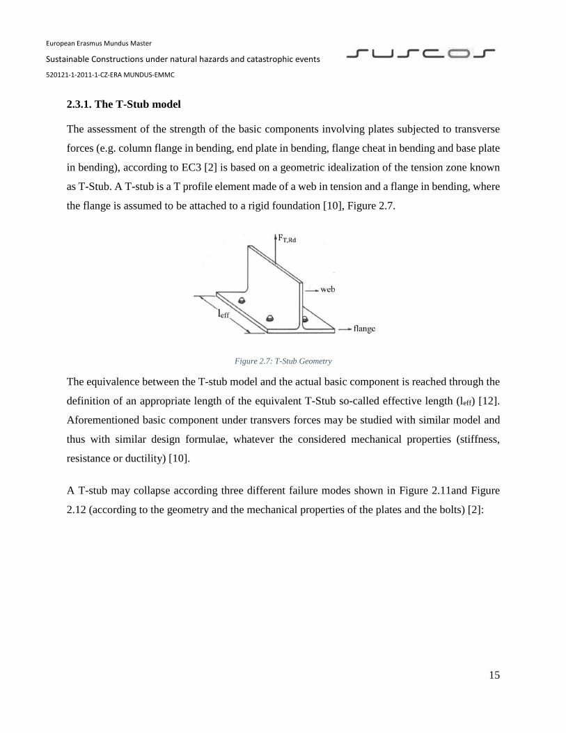
as T-Stub. A T-stub is a T profile element made of a web in tension and a flange in bending, where
the flange is assumed to be attached to a rigid foundation [10], Figure 2.7.
Figure 2.7: T-Stub Geometry
The equivalence between the T-stub model and the actual basic component is reached through the
definition of an appropriate length of the equivalent T-Stub so-called effective length (leff) [12].
Aforementioned basic component under transvers forces may be studied with similar model and
thus with similar design formulae, whatever the considered mechanical properties (stiffness,
resistance or ductility) [10].
A T-stub may collapse according three different failure modes shown in Figure 2.11and Figure
2.12 (according to the geometry and the mechanical properties of the plates and the bolts) [2]:
European Erasmus Mundus Master
Sustainable Constructions under natural hazards and catastrophic events
520121-1-2011-1-CZ-ERA MUNDUS-EMMC
16
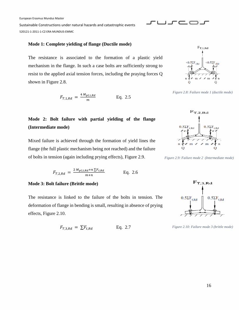
Mode 1: Complete yielding of flange (Ductile mode)
The resistance is associated to the formation of a plastic yield
mechanism in the flange. In such a case bolts are sufficiently strong to
resist to the applied axial tension forces, including the praying forces Q
shown in Figure 2.8.
𝐹𝐹𝑇𝑇,1,𝑅𝑅𝑅𝑅 = 4 𝑀𝑀𝑝𝑝𝑝𝑝,1,𝑅𝑅𝐸𝐸
𝑚𝑚 Eq. 2.5
Mode 2: Bolt failure with partial yielding of the flange
(Intermediate mode)
Mixed failure is achieved through the formation of yield lines the
flange (the full plastic mechanism being not reached) and the failure
of bolts in tension (again including prying effects), Figure 2.9.
𝐹𝐹𝑇𝑇,2,𝑅𝑅𝑅𝑅 = 2 𝑀𝑀𝑝𝑝𝑝𝑝,2,𝑅𝑅𝐸𝐸+𝑛𝑛 ∑𝐹𝐹𝑡𝑡,𝑅𝑅𝐸𝐸
𝑚𝑚+𝑛𝑛 Eq. 2.6
Mode 3: Bolt failure (Brittle mode)
The resistance is linked to the failure of the bolts in tension. The
deformation of flange in bending is small, resulting in absence of prying
effects, Figure 2.10.
𝐹𝐹𝑇𝑇,3,𝑅𝑅𝑅𝑅 = ∑𝐹𝐹𝑡𝑡,𝑅𝑅𝑅𝑅 Eq. 2.7
Figure 2.8: Failure mode 1 (ductile mode)
Figure 2.9: Failure mode 2 (Intermediate mode)
Figure 2.10: Failure mode 3 (brittle mode)

European Erasmus Mundus Master
Sustainable Constructions under natural hazards and catastrophic events
520121-1-2011-1-CZ-ERA MUNDUS-EMMC
17
Figure 2.11: Schematic failure modes of T-Stub [13]
Figure 2.12: Ductile failure mode & Intermediate failure mode in T-Stub profiles [14 ]
Where;
𝐹𝐹𝑇𝑇,𝑅𝑅𝑅𝑅 is the design tension resistance of T-stub
Q is the prying force
𝑀𝑀𝑝𝑝𝑝𝑝,1,𝑅𝑅𝑅𝑅 = 0.25 ∑ 𝑝𝑝𝑒𝑒𝑒𝑒𝑒𝑒,1𝑡𝑡𝑒𝑒
2
𝛾𝛾𝑀𝑀0
𝑀𝑀𝑝𝑝𝑝𝑝,2,𝑅𝑅𝑅𝑅 = 0.25 ∑ 𝑝𝑝𝑒𝑒𝑒𝑒𝑒𝑒,2𝑡𝑡𝑒𝑒
2
𝛾𝛾𝑀𝑀0
n = e min but n ≤ 1.25m
tf is thickness of the T-Stub flange
European Erasmus Mundus Master
Sustainable Constructions under natural hazards and catastrophic events
520121-1-2011-1-CZ-ERA MUNDUS-EMMC
18
fy is the yield strength of the T-Stub flange
𝛾𝛾𝑀𝑀0 is partial safety factor for the resistance of flange (recommended value: 𝛾𝛾𝑀𝑀0 = 1)
∑𝑙𝑙𝑒𝑒𝑒𝑒𝑒𝑒,1 is value of 𝑙𝑙𝑒𝑒𝑒𝑒𝑒𝑒,1for Mode 1
∑𝑙𝑙𝑒𝑒𝑒𝑒𝑒𝑒,2 is value of 𝑙𝑙𝑒𝑒𝑒𝑒𝑒𝑒,2for Mode 2
∑𝐹𝐹𝑡𝑡,𝑅𝑅𝑅𝑅 is the sum of design resistance 𝐹𝐹𝑡𝑡,𝑅𝑅𝑅𝑅 = 0.9 𝐴𝐴𝑠𝑠 𝑒𝑒𝑢𝑢𝑏𝑏𝛾𝛾𝑀𝑀2
of all bolts in T-Stub
As is the tensile stress area of the bolts
fub is the ultimate strength of the bolts
𝛾𝛾𝑀𝑀2 is the partial resistance factor of the bolts (recommended value 𝛾𝛾𝑀𝑀2 = 1.0)
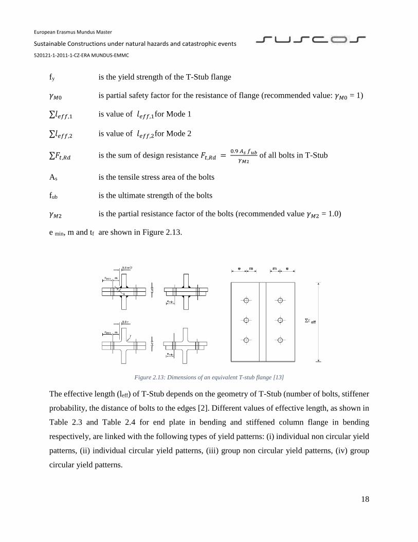
e min, m and tf are shown in Figure 2.13.
Figure 2.13: Dimensions of an equivalent T-stub flange [13]
The effective length (leff) of T-Stub depends on the geometry of T-Stub (number of bolts, stiffener
probability, the distance of bolts to the edges [2]. Different values of effective length, as shown in
Table 2.3 and Table 2.4 for end plate in bending and stiffened column flange in bending
respectively, are linked with the following types of yield patterns: (i) individual non circular yield
patterns, (ii) individual circular yield patterns, (iii) group non circular yield patterns, (iv) group
circular yield patterns.

European Erasmus Mundus Master
Sustainable Constructions under natural hazards and catastrophic events
520121-1-2011-1-CZ-ERA MUNDUS-EMMC
19
Establishment of prying forces in T-Stub leads to individual non circular yield line pattern.
Depending on β values, failure mode 1, 2 or 3 may arise, as shown in Figure 2.14 where
𝛽𝛽 = 4 𝑀𝑀𝑝𝑝𝑝𝑝,1,𝑅𝑅𝐸𝐸
𝑚𝑚∑𝐹𝐹𝑡𝑡,𝑅𝑅𝐸𝐸 = 𝑀𝑀𝑀𝑀𝑅𝑅𝑒𝑒 1
𝑀𝑀𝑀𝑀𝑅𝑅𝑒𝑒 3 Eq. 8
Figure 2.14: Type of failure depending on the geometry of T-Stub [2]
On the other hand, if the prying forces cannot develop in the T-Stub then individual circular yield
line pattern develops. In this scenario failure mode 2 cannot occur, as shown in Figure 2.14.

European Erasmus Mundus Master
Sustainable Constructions under natural hazards and catastrophic events
520121-1-2011-1-CZ-ERA MUNDUS-EMMC
20
Table 2.3: Effective length of end plate [2]
(α should be obtained from Figure 2.15).
Table 2.4: Effective length for stiffened column flange [2]
(α should be obtained from Figure 2.15).
European Erasmus Mundus Master
Sustainable Constructions under natural hazards and catastrophic events
520121-1-2011-1-CZ-ERA MUNDUS-EMMC
21
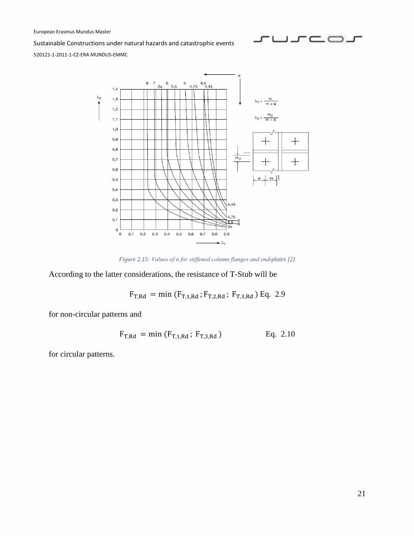
Figure 2.15: Values of α for stiffened column flanges and end-plates [2]
According to the latter considerations, the resistance of T-Stub will be
FT,Rd = min (FT,1,Rd ; FT,2,Rd ; FT,3,Rd ) Eq. 2.9
for non-circular patterns and
FT,Rd = min (FT,1,Rd ; FT,3,Rd ) Eq. 2.10
for circular patterns.

European Erasmus Mundus Master
Sustainable Constructions under natural hazards and catastrophic events
520121-1-2011-1-CZ-ERA MUNDUS-EMMC
22
3. Finite Element Modeling (FEM)
The finite element method (FEM), sometimes refers to a finite element analysis (FEA), is a
powerful tool for computation of complex problems, used to obtain approximate numerical
solutions. FEM is appropriate to problems throughout continuum mechanics, applied mathematics,
engineering, and physics [15].
3.1. FEM elements in ABAQUS
In this dissertation, to assess the cyclic behaviour of stiffened column flange in bending, finite
element models were developed in ABAQUS software, version 6.14 [16]. These models aimed to
perform a parametric analysis to assess the influence of the collapse mode in the cyclic behaviour
of this basic component.
A wide range of variety of elements are used in ABAQUS software for different modelling
analysis. The types of elements available in ABAQUS will be briefly addressed taking into account
the following features [16];
Family
Degree of freedom (directly related to element family)
Number of nodes
Formulation
Integration
Each type of element contains a unique name in ABAQUS software such as T2D2, S4R, or C3D8I.
The elements name classifies aforementioned aspect of an element [16].
3.1.1. Family
One of major distinction between different element families is the geometry type of the elements.
The first letter/letters of an element identify the family that the elements belong, e.g. the C in
C3D8I exhibits this is a continuum element however, the S in S4R exhibits this is a shell element.
Following are commonly used element families, as shown in Figure 3.1.

European Erasmus Mundus Master
Sustainable Constructions under natural hazards and catastrophic events
520121-1-2011-1-CZ-ERA MUNDUS-EMMC
23
Continuum (solid) elements
Shell elements
Beam elements
Rigid elements
Membrane elements
Infinite elements
Spring and dashpots
Truss elements
3.1.2. Degrees of freedom
The degrees of freedom (DOF) are the fundamental variables which are considered during the
resolution of the equilibrium equations. For a stress/displacement analysis, the degrees of freedom
are the translations at each node of each element. Some element families, such as the beam and
shell families, may also have rotational degrees of freedom as well.
3.1.3. Number of nodes (Order of interpolation)
Rotation, displacement, temperature, and other quantities are evaluated only at integration points
of the element. At any other point in the element, these quantities can be obtained from the
integration points through interpolation. Interpolation order is defined by the order of the
polynomial shape functions used for the interpolation, as shown in Figure 3.2.
Figure 3.2: Linear brick, quadratic brick, and modified tetrahedral element [16]
Figure 3.1: Element families in ABAQUS software [16]

European Erasmus Mundus Master
Sustainable Constructions under natural hazards and catastrophic events
520121-1-2011-1-CZ-ERA MUNDUS-EMMC
24
3.1.4. Formulation
An element's formulation denotes to the mathematical theory used to describe the response of an
element. In the absence of adaptive meshing all of the stress/displacement elements in ABAQUS
are based on the Lagrangian or material description of behavior: the material linked with an
element remains linked with the element during the analysis, and material cannot flow across
element boundaries. In the alternative Eulerian or spatial description, elements are fixed in space
as the material flows through them. Eulerian methods are used commonly in fluid mechanics
simulations. ABAQUS/Standard uses Eulerian elements to model convective heat transfer.
Adaptive meshing combines the features of pure Lagrangian and Eulerian analyses and allows the
motion of the element to be independent of the material [16].
To accommodate different types of behavior, some element families in ABAQUS include elements
with several different formulations. For example, the shell element family has three classes: one
suitable for general-purpose shell analysis, another for thin shells, and yet another for thick shells.
Some ABAQUS/Standard element families have a standard formulation as well as some
alternative formulations. Elements with alternative formulations are identified by an additional
character at the end of the element name. For example, the continuum, beam, and truss element
families include members with a hybrid formulation in which the pressure (continuum elements)
or axial force (beam and truss elements) is treated as an additional unknown; these elements are
identified by the letter “H” at the end of the name (C3D8H or B31H).
Some element formulations allow coupled field problems to be solved. For example, elements
whose names begin with the letter C and end with the letter T (such as C3D8T) possess both
mechanical and thermal degrees of freedom and are intended for coupled thermal-mechanical
simulations.
Several are of the most commonly used elements formulation are described in ABAQUS
documentation.

European Erasmus Mundus Master
Sustainable Constructions under natural hazards and catastrophic events
520121-1-2011-1-CZ-ERA MUNDUS-EMMC
25
3.1.5. Integration
ABAQUS software uses numerical system to integrate various quantities over the volume of each
element. ABAQUS evaluates the material response at each integration point in each element. Some
elements can use full or partial integration.
ABAQUS uses the letter “R” at the end of the element name to discriminate reduced-integration
elements (unless they are also hybrid elements, in which case the element name ends with the
letters “RH”), shown in Figure 3.3. For example, CAX4 is the 4-node, fully integrated, linear,
axisymmetric solid element; and CAX4R is the reduced-integration version of the same element.
Figure 3.3: Naming convention of solid elements in ABAQUS [16]
3.2. Solid Elements
The solid (or continuum) elements will be used in this dissertation. These elements are
recommended for complex linear or nonlinear analysis involving contact, plasticity and large
deformations.

European Erasmus Mundus Master
Sustainable Constructions under natural hazards and catastrophic events
520121-1-2011-1-CZ-ERA MUNDUS-EMMC
26
3.2.1. Choosing between quadrilateral and tetrahedral mesh element shapes
With tetrahedral mesh elements it is easy to mesh large complex forms. ABAQUS provides
automatic meshing algorithmic which makes it easy to mesh very complex geometry. Tetrahedral
mesh elements are therefore more suited to mesh complex geometries. However, quadrilateral
mesh element type provides solutions of equal accuracy and at less computer cost. Quadrilateral
mesh elements are more efficient in convergence than tetrahedral mesh elements. Quadrilateral
mesh elements perform better if their shapes are approximately rectangular however tetrahedral
mesh elements don’t depend on initial element geometry.
3.2.2. Choosing between first-order and second-order elements
Second-order elements have higher accuracy in ABAQUS/Standard than first-order elements for
problem solutions that do not involve complex contact conditions, impact, or severe element
alterations. Second order elements capture stress concentrations more efficiently and are better for
modelling structures with complex geometries. First-order triangular and tetrahedral elements
should be avoided in stress analysis problem solution because of the overly stiff nature of elements.
3.3. Material Model in FEM
In this dissertation, for steel profiles including HEA 300, bending plate and stiffener, S420 material
is used while different bolt classes were used. Nominal properties were obtained from EC 3. The
remainder assumed mechanical properties are shown in Table 3.1, Table 3.2, and Table 3.3.
Table 3.1: Elastic properties of material
Density 7.85 x 10⁻⁹ tons/mm3
Young’s modulus 210000 N/mm 2
Poisson ratio 0.3 -

European Erasmus Mundus Master
Sustainable Constructions under natural hazards and catastrophic events
520121-1-2011-1-CZ-ERA MUNDUS-EMMC
27
Table 3.2: Plastic properties of material for mild steel
Material fy (N/mm2) fu (N/mm2) εy εu S 420 420 520 0.02 0.15
Table 3.3: Plastic properties of material for bolts.
Material fy (N/mm2) fu (N/mm2) εy εu 10.9 900 1000 0.02 0.15 8.8 640 800 0.02 0.15 6.8 480 600 0.02 0.15
The material model used for steel in ABAQUS was an elastic-plastic material with isotropic
hardening and associative flow rule. The input for this material model required by ABAQUS is
the uniaxial stress-strain relation.
Since ABAQUS will incorporate the reduction in area by itself due to the Poisson effect, True
Stress-True Strain relations for uniaxial behaviour of steel are required. The stress-strain relation
gathered from coupon tests are valid up to the necking point, after which the materials seems to
soften but it actually hardens because of the fact that after necking significant reduction in cross-
sectional area takes place which results in reduction in material resistance hence the stress values
goes down but actually material continues hardening till fracture.
True Stress-True Strain relations were computed from the engineering stress-strain relations shown
in Figure 3.4 through (Eq. 3.1) and (Eq. 3.2) from EN 1993-1-5. The plastic strain was computed
using Eq. 3.3, where “Ϭtrue” true stress, “Ɛ true” true strain, “Ϭengg” engineering stress, “Ɛengg”
engineering strain, “Ɛ pl” plastic strain and “E” slope of linear elastic range

European Erasmus Mundus Master
Sustainable Constructions under natural hazards and catastrophic events
520121-1-2011-1-CZ-ERA MUNDUS-EMMC
28
Figure 3.4: Stress vs strain
Ϭtrue = ϭ engg (1+ Ɛ) Eq. 3.11
Ɛ true = ln (1+ Ɛengg) Eq. 12
Ɛ pl = ln (1+ Ɛengg) - Ϭ𝑡𝑡𝑟𝑟𝑡𝑡𝑒𝑒𝐸𝐸
Eq. 13
Aforementioned formulas were used up to the maximum load. After the maximum load of
engineering stress, the curve was considered ascending till fracture.
3.4. Constrain and Contact Interaction
In ABAQUS, different components of model interact with each other by continuity links so-called
constraints (e.g. between beam flange and the end plate) or defining contact properties so-called
interactions (e.g. between the end plate and column flange, between bolts and the end plate or
column flange).
The beam flange elements and stiffener elements were constrained to the end plate and column
respectively by a “tie constraint” that use the concept of master and slave nodes to define the same
degree of freedom between both. The column edges elements were constrained with reference
points for supports by “coupling constraint”, using same master and slave philosophy, the degrees
0
200
400
600
800
1000
1200
0 0.02 0.04 0.06 0.08 0.1 0.12 0.14 0.16
Stre
ss (N
/mm
2 )
Strain (ε)
Engineering Stress vs Engineering Strain
S 420
10.9
8.8
6.8
European Erasmus Mundus Master
Sustainable Constructions under natural hazards and catastrophic events
520121-1-2011-1-CZ-ERA MUNDUS-EMMC
29
of freedom of the dependent nodes are eliminated; the two surfaces will have the same values of
their degrees of freedom.
The interaction between the end plate and column flange, and the interaction between bolts and
the column flange or the end plate were imposed by the general contact algorithm, which used
“hard contact” formulation, using the penalty method to approximate the hard pressure overclosure
behaviour (normal behaviour) that acts in the normal direction to resist penetration. Friction
coefficient 0.2 was used to imposed “Tangential behaviour”.
ABAQUS divides the problem history into steps. A step is any convenient phase of the history
and, in its simplest form, a step can be just a static analysis, a load change from a magnitude to
another, an initial pre-stress operation of a part of the structure or the change of a boundary
condition in the model.
In this particular case, the solution of the problem is obtained in 3 steps. The first step is used to
formulate the boundary conditions and prepare the contact interactions defined previously.
The second step corresponds to the pre-loading of the bolts using the adjust length option and
determining the length magnitude by the elastic elongation needed to produce the required amount
of force in the bolts, normally a percentage of the ultimate strength. Figure 3.5 shows the plane
where the adjust length option is applied.
In the third step the bolts current length is fixed so the magnitude is computed during the analyses.
This option allows maintaining the pre-defined load in the bolts during the third step. It is in the
third step that the pushover begins, changing the boundary conditions on the tip of the cantilever
by imposing a displacement in the boundary condition parallel to the beam web.

European Erasmus Mundus Master
Sustainable Constructions under natural hazards and catastrophic events
520121-1-2011-1-CZ-ERA MUNDUS-EMMC
30
Figure 3.5: Bolts pre-loading plane [11]
3.5. Loading
The models were loaded following protocol which consisted of an imposed displacement applied
at the beam flange end, according to scheme shown in Figure 4.5. All models were prepared to
deal with monotonic loads and cyclic loads. The “loads” were applied in a displacement control
approach, i.e. a displacement is imposed at the tip of beam flange, see Figure 4.5. The loading
protocol is defined by the direction (along the three global axis, although in this dissertation only
the YY axis direction was used), with same orientation but for cyclic loads, amplitude of the
displacement and number of cycles are detail discussed in next chapter.
European Erasmus Mundus Master
Sustainable Constructions under natural hazards and catastrophic events
520121-1-2011-1-CZ-ERA MUNDUS-EMMC
31
4. Numerical Model
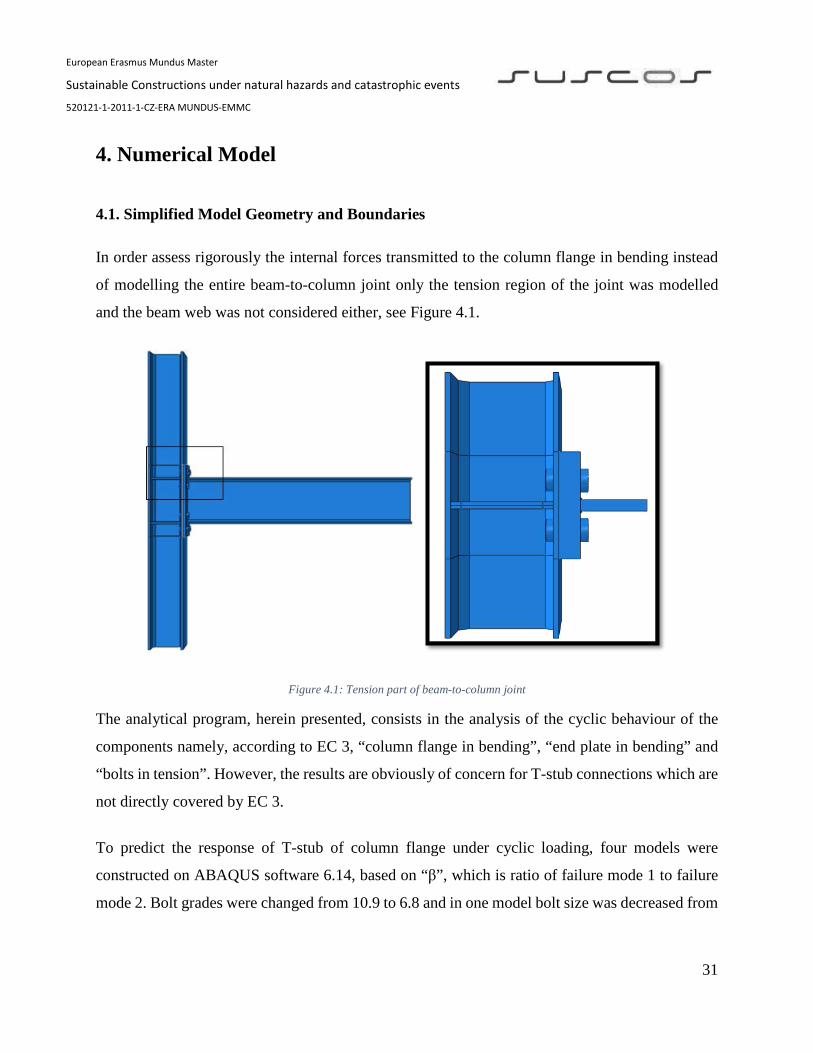
4.1. Simplified Model Geometry and Boundaries
In order assess rigorously the internal forces transmitted to the column flange in bending instead
of modelling the entire beam-to-column joint only the tension region of the joint was modelled
and the beam web was not considered either, see Figure 4.1.
Figure 4.1: Tension part of beam-to-column joint
The analytical program, herein presented, consists in the analysis of the cyclic behaviour of the
components namely, according to EC 3, “column flange in bending”, “end plate in bending” and
“bolts in tension”. However, the results are obviously of concern for T-stub connections which are
not directly covered by EC 3.
To predict the response of T-stub of column flange under cyclic loading, four models were
constructed on ABAQUS software 6.14, based on “β”, which is ratio of failure mode 1 to failure
mode 2. Bolt grades were changed from 10.9 to 6.8 and in one model bolt size was decreased from

European Erasmus Mundus Master
Sustainable Constructions under natural hazards and catastrophic events
520121-1-2011-1-CZ-ERA MUNDUS-EMMC
32
M36 to M30 with grade 10.9 to achieve different mode ratios. Whole model is consisting of column
profile (HEA 300), bending plate, stiffeners, and bolts, see in Figure 4.2.
Figure 4.2: 3D view of the tension region of the beam-column joint
4.2. Parametric Analysis
The parametric analysis performed aimed to assess the influence of the ratio between the mode 1
and mode 2 of the failure loads of the T-stub corresponding of column flange in bending according
to EC 3-1-8 model. Accordingly, a ratio β was considered
𝛽𝛽 = 𝐹𝐹𝑇𝑇,1 𝐹𝐹𝑇𝑇,2,
Eq. 14.1

European Erasmus Mundus Master
Sustainable Constructions under natural hazards and catastrophic events
520121-1-2011-1-CZ-ERA MUNDUS-EMMC
33
where FT,1 and FT,1 were computed using expressions Eq. 2.5 and Eq. 2.6, respectively. Bolt
grades were changed from 10.9 to 6.8 and in one model bolt size was decreased from M36 to M30
with grade 10.9 to achieve different mode ratios. Whole model is consisting of column profile
(HEA 300), bending plate, stiffeners, beam flange and bolts, see Figure 4.2.
The models were also defined in order that the failure mode 3 in column flange in bending is
always higher than the lower of failure modes 1 and 2. The end plate thickness and the beam flange
was also defined to be strong enough to avoid failure modes 1 and 2 in the end plate as well as in
the beam flange in tension.
4.3. FEM Model Construction
A brief description of model construction in ABAQUS is presented in the following sections
together with some more details about the models.
4.3.1. Part Module
In this module, geometry of each part of the model was defined independently using the measures
provided in Figure 4.3. the model comprises 5 parts that were drawn independently using the
procedure shown in Table 4.1.
Table 4.1: Description of the procedures used to draw the parts of the model.
Modelling space 3D Type Deformation Base feature Shape Solid
Type Extrusion

European Erasmus Mundus Master
Sustainable Constructions under natural hazards and catastrophic events
520121-1-2011-1-CZ-ERA MUNDUS-EMMC
34
Figure 4.3: Geometrical description of the components
4.3.2. Property Module
In property module, the material model described in section 3.3 are assigned to each part of the
model according to Table 4.2.
Table 4.2: Material assigned to the parts of the model
Material properties Component of the model
S 450 HEA 300 End plate
10.9 Grade M36/M30 8.8 Grade M36 6.8 Grade M36

European Erasmus Mundus Master
Sustainable Constructions under natural hazards and catastrophic events
520121-1-2011-1-CZ-ERA MUNDUS-EMMC
35
Elastic and plastic properties of material were also introduced in this module, discussed in previous
chapter.
4.3.3. Assembly Module
Each component´s geometry was defined independently, for the assembly of T-stub components,
this module was used, shown in following Figure 4.4.
Figure 4.4: Description of assembly module of a model.
4.3.4. Step Module
Standard general-static step was used to analysis the response of T-stub under monotonic loading
condition and cyclic loading condition.
History output request manager used to identify force and displacement at a specific point in beam
flange.
ABAQUS divides the problem history into steps. A step is any convenient phase of the history
and, in its simplest form, a step can be just a static analysis, a load change from a magnitude to

European Erasmus Mundus Master
Sustainable Constructions under natural hazards and catastrophic events
520121-1-2011-1-CZ-ERA MUNDUS-EMMC
36
another, an initial pre-stress operation of a part of the structure or the change of a boundary
condition in the model.
In this particular case, the solution of the problem is obtained in 3 steps. The first step is used to
formulate the boundary conditions and prepare the contact interactions defined previously.
The second step corresponds to the pre-loading of the bolts using the adjust length option and
determining the length magnitude by the elastic elongation needed to produce the required amount
of force in the bolts, normally a percentage of the ultimate strength. Figure 3.5 shows the plane
where the adjust length option is applied.
In the third step the bolts current length is fixed so the magnitude is computed during the analyses.
This option allows maintaining the pre-defined load in the bolts during the third step. It is in the
third step that the pushover begins, changing the boundary conditions on the tip of the cantilever
by imposing a displacement in the boundary condition parallel to the beam web.
4.3.5. Interaction Module
The models were comprised of many parts presented in Figure 4.2, those parts were interacted
with each other through constraints and/or interactions.
For bolt to steel surface (end plate and HEA 300) and end plate to HEA 300, general contact was
used with friction coefficient of 0.2 in tangential behaviour and hard contact was used for
specifying normal behaviour in contact property option.
Coupling and tie constraints were adopted for boundaries definition and welded parts (beam flange
to end plate and stiffener to column profile) respectively.
Three reference points were selected from model and were coupled using kinematic coupling type
with all degree of freedom constrained with surface of T-stub, shown in Figure 4.5.

European Erasmus Mundus Master
Sustainable Constructions under natural hazards and catastrophic events
520121-1-2011-1-CZ-ERA MUNDUS-EMMC
37
Figure 4.5: Description of interaction module of a model.
4.3.6. Load Module
The reference points RP1 and RP2 were restrained using displacement/rotation boundary type with
all the displacements and rotation fixed. The reference point RP3 was allowed to have a uniform
displacement along the Y-axis of the model, see Figure 4.6.
The displacement in RP3 was increased monotonically until failure of the model for monotonic
loading condition. For cyclic loading condition the loading protocol presented in section 4.4 was
imposed in RP3.
To minimize the lack of convergence issues encountered a preload was assign to the bolts detail
discussed in 3.4 section.

European Erasmus Mundus Master
Sustainable Constructions under natural hazards and catastrophic events
520121-1-2011-1-CZ-ERA MUNDUS-EMMC
38
Figure 4.6: Description of load module of a model.
4.3.7. Mesh Module
The C3D8R linear brick element with 8-node, reduced integration, hourglass control of the
ABAQUS element library was used for meshing all of the components of the models. To overcome
the hourglass issue at least 2 layers were considered in the thickness of the end plates and column
flanges of the models, shown in Figure 4.7. Approximate global size of 10 mm [11], was used for
all components but around bolt holes, mesh size was reduced to avoid convergence problems.
Figure 4.7 shows the meshes used in all the parts of the model

European Erasmus Mundus Master
Sustainable Constructions under natural hazards and catastrophic events
520121-1-2011-1-CZ-ERA MUNDUS-EMMC
39
Figure 4.7: FEM mesh of the parts of the model, a) end plate, b) HEA 300, c) beam flange, d) bolt, and e) stiffener
4.3.8. Visualization Module
The visualization module was used for getting response of the models. Equivalent plastic strain
(PEEQ) and maximum stress (S, Mises) provided by ABAQUS are shown in Figure 4.8 and Force
- Displacement relationship is shown in Figure 4.9.
.

European Erasmus Mundus Master
Sustainable Constructions under natural hazards and catastrophic events
520121-1-2011-1-CZ-ERA MUNDUS-EMMC
40
Figure 4.8: Von Misses stresses and equivalent plastic strains visualization in visualization module of ABAQUS.
Figure 4.9: Force displacement curve in visualization module of ABAQUS
4.2. Loading Protocol
For computation of cyclic behaviour of joints in MRFs, quasi-static loading protocol has been
defined in the EQUALJOINTS project in terms of interstorey drifts. These drifts were computed
based in drift demands from nonlinear time history analyses of moment resisting frames (MRFs),
0
500
1000
1500
2000
2500
3000
0 2 4 6 8 10 12 14 16
Forc
e (k
N)
Deformation (mm)
Force vs Deformation

European Erasmus Mundus Master
Sustainable Constructions under natural hazards and catastrophic events
520121-1-2011-1-CZ-ERA MUNDUS-EMMC
41
dual eccentrically braced frames (D-EBFs) and dual concentrically braced frame (D-CBFs)
typologies [3]. The simplified protocol is given in Table 4.3.
Table 4.3: Simplified loading protocol [3]
no. of
cycles
drift angle θ
(rad)
6 0.004
6 0.006
4 0.010
2 0.015
2 0.020
2 0.030
2 0.040
The protocol can be continued after the maximum cycle of 0.040 rad by further loading at
increments of 0.01 rad, with two cycles of loading at each step, as long as the state of the specimen
permit.
Assuming in the safe side that [3]:
(i) The entire drift arises from the connection, i.e. the beam and columns are rigid and there
is no deformation in the CWS;
(ii) The connection internal arm is “z” (assume it to be equal to the distance between the beam
flange centerlines; 435.4 mm);
(iii) Compression components deformation is negligible (compression components are much
stiffer than the tensile components);
The relation between the maximum drift angle (θ) and the deformation in the tension components
(δ) is δ = z × tan (θ) and the compression deformation is null. Accordingly, the load quasi static
load protocol to is considered in Table 4 4 and is represented in Figure 4.10.

European Erasmus Mundus Master
Sustainable Constructions under natural hazards and catastrophic events
520121-1-2011-1-CZ-ERA MUNDUS-EMMC
42
Table 4 4: Loading protocol for the T-stub [3]
no. of
cycles
maximum tensile
deformation z (m)
6 z × tan(0.004)
6 z × tan(0.006)
4 z × tan(0.010)
2 z × tan(0.015)
2 z × tan(0.020)
2 z × tan(0.030)
2 z × tan(0.040)
δ
...number of cycles
z tan(0.004)z tan(0.006)z tan(0.010)z tan(0.015)
Figure 4.10: Loading protocol for a T-stub [3]

European Erasmus Mundus Master
Sustainable Constructions under natural hazards and catastrophic events
520121-1-2011-1-CZ-ERA MUNDUS-EMMC
43
5. Results and Discussion
In this section, the full details about the models are provided and the monotonic and cyclic analysis
of their behaviour and the column flange in particular is presented.
5.1. FEM Models Definition
Four models were built in ABAQUS for different values of β for column flange in bending in the
range [0.75;1.25]. These models were obtained by changing the material and geometrical
properties of bolts.
Having into account the EC3-1-8 provisions presented in section 2.3.1, for the geometry
represented in Figure 4.3, only plastic collapse mechanism for individual bolts are possible and
thus for the computation of the effective length of the T-stub the bolts need only to be considered
individually – with circular and non-circular patterns for the yield lines. Accordingly, Table 5.1
presents the effective length for the column flange in bending.
Table 5.1: Effective length for a stiffened column flange in a bolted connection.
Bolt row location
Bolt row considered individually
Circular patterns leff, cp (mm)
Non circular patterns
leff, nc (mm)
Bolt row adjacent to a stiffener 2πm αm
274.89 262.5 For Mode 1: l eff, 1 = l eff, nc but l eff, 1 ≤ l eff, cp 262.5 For Mode 2: l eff, 2 = l eff, nc 262.5
m = 43.75 mm e1 = 75 mm m2 = 52 mm λ1 = m/(m+e) 0.4 α = 6
Tables 5.3, 5.4, 5.5 and 5.6 present the mechanical properties and the bolt sizes for the models
considered in the parametric analysis. These tables also present the strength of these models for
the three collapse modes considered in EC3-1-8 for the T-Stub model.
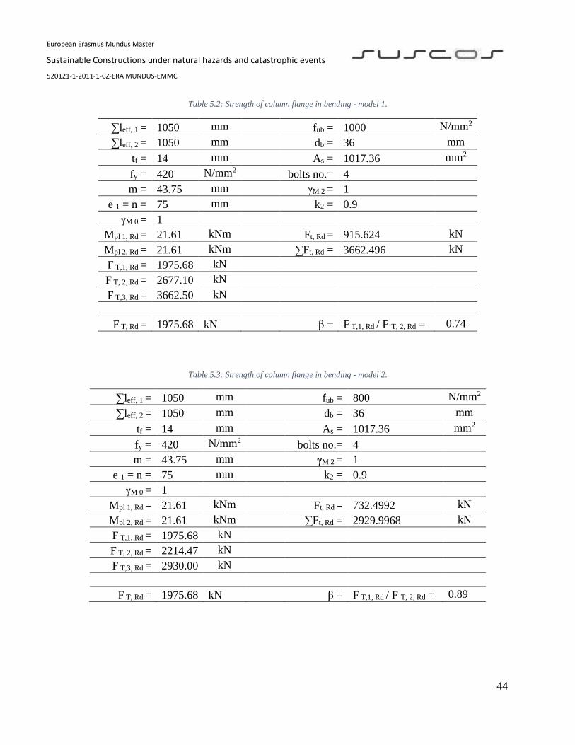
European Erasmus Mundus Master
Sustainable Constructions under natural hazards and catastrophic events
520121-1-2011-1-CZ-ERA MUNDUS-EMMC
44
Table 5.2: Strength of column flange in bending - model 1.
∑leff, 1 = 1050 mm fub = 1000 N/mm2 ∑leff, 2 = 1050 mm db = 36 mm
tf = 14 mm As = 1017.36 mm2 fy = 420 N/mm2 bolts no.= 4 m = 43.75 mm γM 2 = 1
e 1 = n = 75 mm k2 = 0.9 γM 0 = 1
Mpl 1, Rd = 21.61 kNm Ft, Rd = 915.624 kN Mpl 2, Rd = 21.61 kNm ∑Ft, Rd = 3662.496 kN F T,1, Rd = 1975.68 kN F T, 2, Rd = 2677.10 kN F T,3, Rd = 3662.50 kN
F T, Rd = 1975.68 kN β = F T,1, Rd / F T, 2, Rd = 0.74
Table 5.3: Strength of column flange in bending - model 2.
∑leff, 1 = 1050 mm fub = 800 N/mm2 ∑leff, 2 = 1050 mm db = 36 mm
tf = 14 mm As = 1017.36 mm2 fy = 420 N/mm2 bolts no.= 4 m = 43.75 mm γM 2 = 1
e 1 = n = 75 mm k2 = 0.9 γM 0 = 1
Mpl 1, Rd = 21.61 kNm Ft, Rd = 732.4992 kN Mpl 2, Rd = 21.61 kNm ∑Ft, Rd = 2929.9968 kN F T,1, Rd = 1975.68 kN F T, 2, Rd = 2214.47 kN F T,3, Rd = 2930.00 kN
F T, Rd = 1975.68 kN β = F T,1, Rd / F T, 2, Rd = 0.89
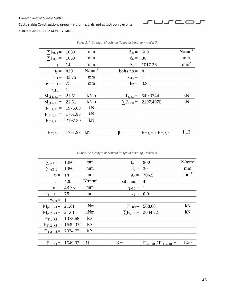
European Erasmus Mundus Master
Sustainable Constructions under natural hazards and catastrophic events
520121-1-2011-1-CZ-ERA MUNDUS-EMMC
45
Table 5.4: Strength of column flange in bending - model 3.
∑leff, 1 = 1050 mm fub = 600 N/mm2 ∑leff, 2 = 1050 mm db = 36 mm
tf = 14 mm As = 1017.36 mm2 fy = 420 N/mm2 bolts no.= 4 m = 43.75 mm γM 2 = 1
e 1 = n = 75 mm k2 = 0.9 γM 0 = 1
Mpl 1, Rd = 21.61 kNm Ft, Rd = 549.3744 kN Mpl 2, Rd = 21.61 kNm ∑Ft, Rd = 2197.4976 kN F T,1, Rd = 1975.68 kN F T, 2, Rd = 1751.83 kN F T,3, Rd = 2197.50 kN
F T, Rd = 1751.83 kN β = F T,1, Rd / F T, 2, Rd = 1.13
Table 5.5: Strength of column flange in bending - model 4.
∑leff, 1 = 1050 mm fub = 800 N/mm2 ∑leff, 2 = 1050 mm db = 30 mm
tf = 14 mm As = 706.5 mm2 fy = 420 N/mm2 bolts no.= 4 m = 43.75 mm γM 2 = 1
e 1 = n = 75 mm k2 = 0.9 γM 0 = 1
Mpl 1, Rd = 21.61 kNm Ft, Rd = 508.68 kN Mpl 2, Rd = 21.61 kNm ∑Ft, Rd = 2034.72 kN F T,1, Rd = 1975.68 kN F T, 2, Rd = 1649.03 kN F T,3, Rd = 2034.72 kN
F T, Rd = 1649.03 kN β = F T,1, Rd / F T, 2, Rd = 1.20

European Erasmus Mundus Master
Sustainable Constructions under natural hazards and catastrophic events
520121-1-2011-1-CZ-ERA MUNDUS-EMMC
46
As already pointed out, to minimize the interaction between the failures modes of the column
flange in bending and the failure of the remainder components, the remainder components were
made stronger than the column flange in bending. In particular, the beam end plate was defined
thick enough to guarantee that the lower collapse mode according to the T-stub model is the mode
3. Table 5.6 presents the computation of the effective length for the beam end plate and Tables
5.7, 5.8, 5.9 and 5.10 represent the strength of the three collapse models of the corresponding T-
stub model showing that, for each model, the strength of collapse mode 1 and 2 in the beam end
plate is always greater than the strength of mode 3 and is always greater than the strength of the
weakest collapse modes of the column flange in bending.
Table 5.6: Effective length for end plate in a bolted connection
Bolt-row location
Bolt row considered individually
Circular patterns leff, cp (mm)
Non circular patterns leff, nc (mm)
Bolt row outside tension
flange of beam
Smallest of: 2πmx πmx + w πmx + 2e
Smallest of: 4mx + 1.25ex e+2mx + 0.625ex 0.5bp 0.5w + 2mx + 0.625ex
285.77 150 For Mode 1: l eff, 1 = l eff, nc but l eff, 1 ≤ l eff, cp 150 For Mode 2: l eff, 2 = l eff, nc 150 mx = 46.4 mm w = 150 mm ex = 70 mm bp = 300 mm

European Erasmus Mundus Master
Sustainable Constructions under natural hazards and catastrophic events
520121-1-2011-1-CZ-ERA MUNDUS-EMMC
47
Table 5.7: Strength of beam end plate - model 1.
∑leff, 1 = 600 mm fub = 1000 N/mm2 ∑leff, 2 = 600 mm db = 36 mm
tf = 55 mm As = 1017.36 mm2 ff = 420 N/mm2 bolts no.= 4 m = 46.4 mm γM 2 = 1
e x = n = 70 mm k2 = 0.9 γM 0 = 1
Mpl 1, Rd = 190.58 kNm Ft, Rd = 915.624 kN Mpl 2, Rd = 190.58 kNm ∑Ft, Rd = 3662.496 kN F T,1, Rd = 16428.88 kN F T, 2, Rd = 5477.02 kN F T,3, Rd = 3662.50 kN
F T, Rd = 3662.50 kN
Table 5.8: Strength of beam end plate - model 2.
∑leff, 1 = 600 mm fub = 800 N/mm2 ∑leff, 2 = 600 mm db = 36 mm
tf = 55 mm As = 1017.36 mm2 ff = 420 N/mm2 bolts no.= 4 m = 46.4 mm γM 2 = 1
e x = n = 70 mm k2 = 0.9 γM 0 = 1
Mpl 1, Rd = 190.58 kNm Ft, Rd = 732.4992 kN Mpl 2, Rd = 190.58 kNm ∑Ft, Rd = 2929.9968 kN F T,1, Rd = 16428.88 kN F T, 2, Rd = 5036.51 kN F T,3, Rd = 2930.00 kN
F T, Rd = 2930.00 kN

European Erasmus Mundus Master
Sustainable Constructions under natural hazards and catastrophic events
520121-1-2011-1-CZ-ERA MUNDUS-EMMC
48
Table 5.9: Strength of beam end plate - model 3.
∑leff, 1 = 600 mm fub = 600 N/mm2 ∑leff, 2 = 600 mm db = 36 mm
tf = 55 mm As = 1017.36 mm2 ff = 420 N/mm2 bolts no.= 4 m = 46.4 mm γM 2 = 1
e x = n = 70 mm k2 = 0.9 γM 0 = 1
Mpl 1, Rd = 190.58 kNm Ft, Rd = 549.3744 kN Mpl 2, Rd = 190.58 kNm ∑Ft, Rd = 2197.4976 kN F T,1, Rd = 16428.88 kN F T, 2, Rd = 4596.00 kN F T,3, Rd = 2197.50 kN
F T, Rd = 2197.50 kN
Table 5.10: Strength of beam end plate - model 4.
∑leff, 1 = 600 mm fub = 1000 N/mm2 ∑leff, 2 = 600 mm db = 30 mm
tf = 55 mm As = 706.5 mm2 ff = 420 N/mm2 bolts no.= 4 m = 46.4 mm γM 2 = 1
e x = n = 70 mm k2 = 0.9 γM 0 = 1
Mpl 1, Rd = 190.58 kNm Ft, Rd = 635.85 kN Mpl 2, Rd = 190.58 kNm ∑Ft, Rd = 2543.4 kN F T,1, Rd = 16428.88 kN F T, 2, Rd = 4804.02 kN F T,3, Rd = 2543.40 kN
F T, Rd = 2543.40 kN
European Erasmus Mundus Master
Sustainable Constructions under natural hazards and catastrophic events
520121-1-2011-1-CZ-ERA MUNDUS-EMMC
49
5.2. Monotonic Behaviour
For monotonically loaded models, an imposed displacement was applied in the boundary
conditions as described in previous chapter, the solution was obtained in 3 steps.
First step was used to formulate the boundary conditions and interactions, as explained in the
previous chapters. The second step was used to for the pre-loading of the bolts, using the adjust
length option and calculation the length magnitude by the elastic elongation needed to simulate
the required amount of force in the bolts, 80 % of the bolt yield axial force was used. Finally, in
third step, a pushover analysis was performed.
5.2.3. Column Flange in Bending
The main objective of monotonic analysis was to compare the strength of the column flange in
bending of the FEM with strength to be expected according to the T-stub model from EC3-1-8 and
presented in section 5.2.1.
During the course this work was not possible to reach the collapse of the FEM models due to
convergence issues. Accordingly, the strength computed according to EC3-1-8 was compared with
the internal force corresponding to the end of the elastic regime in the FEM models.
To identify the response of column flange models from numerical analysis, applied monotonic
loads were gathered from the FEM model and deformation (δ) of T-stub models were computed
by subtracting the deformation (U) at column´s web from the average deformation (U1+U2)/2 at
bolt holes, shown in Figure 5.1 has suggested by Hugo [11].

European Erasmus Mundus Master
Sustainable Constructions under natural hazards and catastrophic events
520121-1-2011-1-CZ-ERA MUNDUS-EMMC
50
Figure 5.1: Predefine nodes to assess the deformation of column flange in bending [11]
The force corresponding to the elastic regime was assumed to correspond to the point of
intersection of the two straight lines arising from bilinear approximation [17] of the force
displacement curves, shown in Figure 5.2, Figure 5.3, Figure 5.4, and Figure 5.5 - the bilinear
approximation was derived through regression analysis. For regression analysis, two lines were
drawn, blue and orange lines, on a Force-Deformation curved of models, taking into account that
blue line should characterize the part of the load-deformation curve before the yielding
(approximately 55% of maximum load, obtained through F-δ curve) and the orange line should
characterize the part of the curve after the yielding.
Figure 5.6 compares the monotonic behaviour of the column flange in bending from all the models
and Table 5.11 shows the comparison of the elastic limit computed as mentioned in the formed
paragraph with the strength of the column flange in bending computed using the T-Stub model for
EC3-1-8.

European Erasmus Mundus Master
Sustainable Constructions under natural hazards and catastrophic events
520121-1-2011-1-CZ-ERA MUNDUS-EMMC
51
Figure 5.2: Force-Deformation curve and bilinear approximation for the column flange in bending in model 1
Figure 5.3: Force-Deformation curve and bilinear approximation for the column flange in bending in model 2
y = 1755.2x
y = 91.178x + 1270.5
0
500
1000
1500
2000
2500
3000
0 2 4 6 8 10 12 14 16 18
Forc
e (k
N)
Deformation of column flange (mm)1 2 Linear (1) Linear (1)
y = 1461.1x
y = 80.541x + 1263.3
0
500
1000
1500
2000
2500
3000
0 2 4 6 8 10 12 14 16 18
Forc
e (k
N)
Deformation of column flange in bending (mm)1 2 Linear (1) Linear (2)

European Erasmus Mundus Master
Sustainable Constructions under natural hazards and catastrophic events
520121-1-2011-1-CZ-ERA MUNDUS-EMMC
52
Figure 5.4: Force-Deformation curve and bilinear approximation for the column flange in bending in model 3
Figure 5.5: Force-Deformation curve and bilinear approximation for the column flange in bending in model 4
y = 1718.3x
y = 90.026x + 1194.3
0
500
1000
1500
2000
2500
3000
0 2 4 6 8 10 12 14 16 18
Forc
e (k
N)
Deformation of column flange in bending (mm)1 2 Linear (1) Linear (2)
y = 1494.1x
y = 85.286x + 1154.1
0
500
1000
1500
2000
2500
3000
0 2 4 6 8 10 12 14 16 18
Forc
e (k
N)
Deformation of column flange in bending (mm)1 2 Linear (1) Linear (2)

European Erasmus Mundus Master
Sustainable Constructions under natural hazards and catastrophic events
520121-1-2011-1-CZ-ERA MUNDUS-EMMC
53
Figure 5.6: Force-Deformation curves for the column flange in bending
Table 5.11: Comparison of T-stub response obtained from EC3-1-3 and numerical models
Model Bolt Failure Mode
EC3-1-8 Analytical Results Deviation
Ft, Rd (kN) β Ft, Rd (kN) % 1 M36 (10.9) Mode 1 1975.68 0.74 1341.12 32.17 2 M36 (8.8) Mode 1 1975.68 0.89 1337.00 32.33 3 M36 (6.8) Mode 2 1751.83 1.13 1260.51 28.05 4 M30 (10.9) Mode 2 1649.03 1.2 1223 25.78
Having into account that the T-Stub models considered in EC3-1-8 rely in the formation of a plastic
mechanism to compute their strength it is expected that the strength computed using these
simplified T-Stub models to be higher than the force corresponding to the end of the elastic regime
computed as explained previously and shown in Figure 5.2, Figure 5.3, Figure 5.4, and Figure 5.5.
The results in Table 5.11 confirm these expectation showing that the strength computed from the
T-Stub models is 25 to 35% higher than the force corresponding to the end of the elastic regime
of the column flange in bending in the FEM models.
0
500
1000
1500
2000
2500
3000
0 2 4 6 8 10 12 14 16 18
Forc
e (k
N)
Deformation of column flange in bending (mm)
Force vs Deformation
Model 1 Model 2 Model 3 Model 4

European Erasmus Mundus Master
Sustainable Constructions under natural hazards and catastrophic events
520121-1-2011-1-CZ-ERA MUNDUS-EMMC
54
Figure 5.6 shows that the smaller the β, the stiffer the column flange in bending, however the
differences between the four models are small. To assess the influence of the β parameter in the
shape of the force-deformation relation of the column flange in bending the curves shown in Figure
5.6 was normalizing by getting the maximum forces of each curves in the range [0, 10] mm and
dividing the forces in that range by that force, see Figure 5.7. It reveals that no huge variances are
to be predicted from the normalized curves.
Figure 5.7: Normalized Force-Deformation curves for monotonically loaded models
0.00
0.20
0.40
0.60
0.80
1.00
0 2 4 6 8 10
F/F m
ax
Deformation of column flange in bending (mm)
Model 1 Model 2 Model 3 Model 4
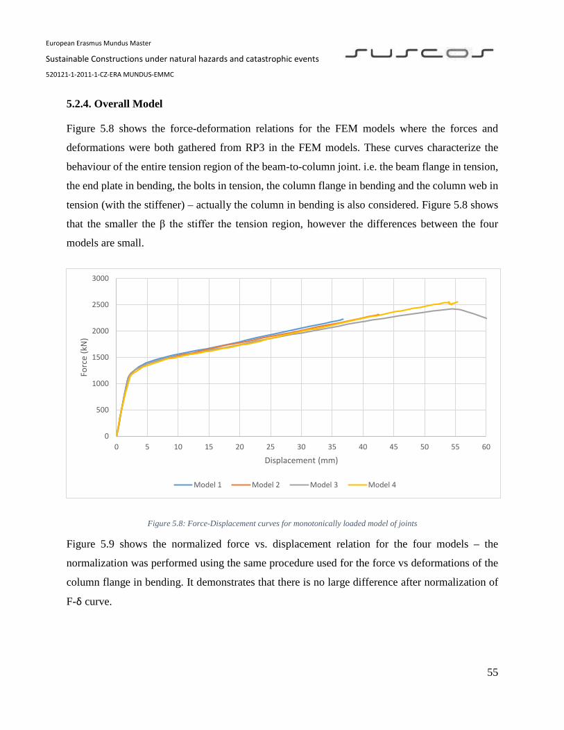
European Erasmus Mundus Master
Sustainable Constructions under natural hazards and catastrophic events
520121-1-2011-1-CZ-ERA MUNDUS-EMMC
55
5.2.4. Overall Model
Figure 5.8 shows the force-deformation relations for the FEM models where the forces and
deformations were both gathered from RP3 in the FEM models. These curves characterize the
behaviour of the entire tension region of the beam-to-column joint. i.e. the beam flange in tension,
the end plate in bending, the bolts in tension, the column flange in bending and the column web in
tension (with the stiffener) – actually the column in bending is also considered. Figure 5.8 shows
that the smaller the β the stiffer the tension region, however the differences between the four
models are small.
Figure 5.8: Force-Displacement curves for monotonically loaded model of joints
Figure 5.9 shows the normalized force vs. displacement relation for the four models – the
normalization was performed using the same procedure used for the force vs deformations of the
column flange in bending. It demonstrates that there is no large difference after normalization of
F-δ curve.
0
500
1000
1500
2000
2500
3000
0 5 10 15 20 25 30 35 40 45 50 55 60
Forc
e (k
N)
Displacement (mm)
Model 1 Model 2 Model 3 Model 4
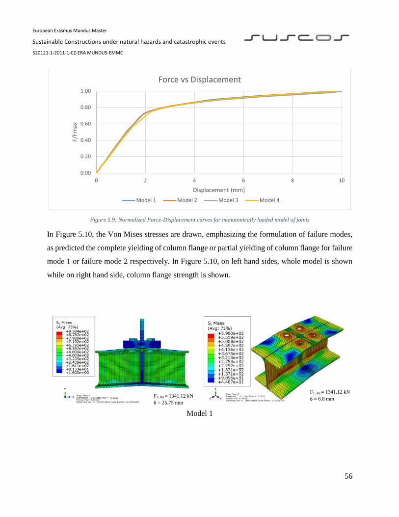
European Erasmus Mundus Master
Sustainable Constructions under natural hazards and catastrophic events
520121-1-2011-1-CZ-ERA MUNDUS-EMMC
56
Figure 5.9: Normalized Force-Displacement curves for monotonically loaded model of joints
In Figure 5.10, the Von Mises stresses are drawn, emphasizing the formulation of failure modes,
as predicted the complete yielding of column flange or partial yielding of column flange for failure
mode 1 or failure mode 2 respectively. In Figure 5.10, on left hand sides, whole model is shown
while on right hand side, column flange strength is shown.
Model 1
0.00
0.20
0.40
0.60
0.80
1.00
0 2 4 6 8 10
F/Fm
ax
Displacement (mm)
Force vs Displacement
Model 1 Model 2 Model 3 Model 4
FT, Rd = 1341.12 kN δ = 6.8 mm FT, Rd = 1341.12 kN
δ = 25.75 mm

European Erasmus Mundus Master
Sustainable Constructions under natural hazards and catastrophic events
520121-1-2011-1-CZ-ERA MUNDUS-EMMC
57
Model 2
Model 3
Model 4
Figure 5.10:Von Mises stress for monotonically loaded models
FT, Rd = 1337.00 kN δ = 24.14 mm
FT, Rd = 1337.00 kN δ = 7.25 mm
FT, Rd = 1260.51 kN δ = 6.53 mm
FT, Rd = 1260.51 kN δ = 22.34 mm
FT, Rd = 1223 kN δ = 21.25 mm
FT, Rd = 1223 kN δ = 7.09 mm

European Erasmus Mundus Master
Sustainable Constructions under natural hazards and catastrophic events
520121-1-2011-1-CZ-ERA MUNDUS-EMMC
58
5.3. Cyclic Behaviour
The cyclic analysis of the FEM models followed the same procedure as described for
monotonically loaded models. The load history was applied imposing the load protocol described
in section 4.2 to the RP3.
Again, due to convergence issues, in the course of the present work it was not possible to reach
the collapse of the models. This way, the cyclic behavior of the models was studied only for the
first 24 cycles of the loading protocol defined in section 3.5.
5.3.1. Column Flange in Bending
Figure 5.11, Figure 5.12, Figure 5.13, and Figure 5.14 show the cyclic and the monotonic force
vs. deformation of the column flange in bending of the four models described in section 5.1.
Figure 5.11: Force-Deformation curves for the column flange in bending under cyclic and monotonic loads – model 1.
-2000
-1500
-1000
-500
0
500
1000
1500
2000
0 0.25 0.5 0.75 1 1.25 1.5 1.75 2 2.25 2.5 2.75 3
Forc
e (k
N)
Deformation of the column flange in bending (mm)
Model 1 under cyclic load Model 1 under monotonic load

European Erasmus Mundus Master
Sustainable Constructions under natural hazards and catastrophic events
520121-1-2011-1-CZ-ERA MUNDUS-EMMC
59
Figure 5.12: Force-Deformation curves for the column flange of Model 2 under cyclic and monotonic loads
Figure 5.13: Force-Deformation curves for the column flange of Model 3 under cyclic and monotonic loads
-2000
-1500
-1000
-500
0
500
1000
1500
2000
0 0.5 1 1.5 2 2.5 3
Forc
e (k
N)
Deformation of the column flange in bending (mm)
Model 2 under cyclic load Model 2 under monotonic load
-2000
-1500
-1000
-500
0
500
1000
1500
2000
0 0.25 0.5 0.75 1 1.25 1.5 1.75 2 2.25 2.5 2.75 3
Forc
e (k
N)
Deformation of column flange in bending (mm)
Model 3 under cyclic load Model 3 under monotonic load
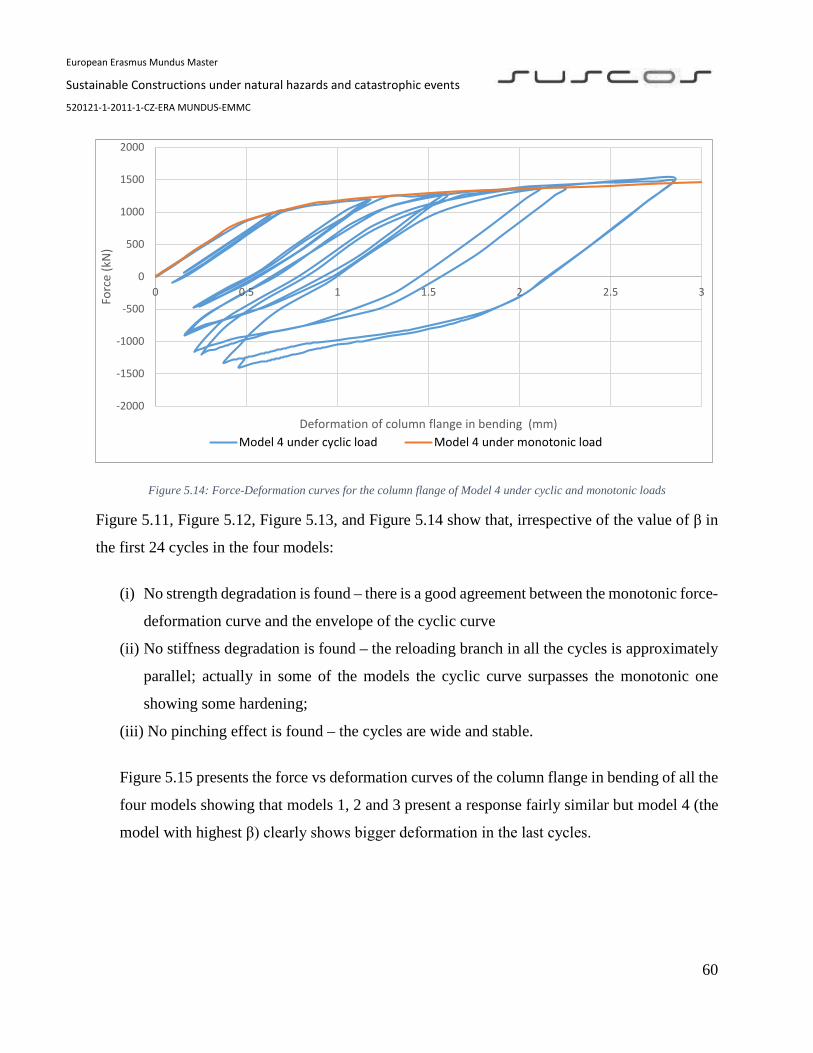
European Erasmus Mundus Master
Sustainable Constructions under natural hazards and catastrophic events
520121-1-2011-1-CZ-ERA MUNDUS-EMMC
60
Figure 5.14: Force-Deformation curves for the column flange of Model 4 under cyclic and monotonic loads
Figure 5.11, Figure 5.12, Figure 5.13, and Figure 5.14 show that, irrespective of the value of β in
the first 24 cycles in the four models:
(i) No strength degradation is found – there is a good agreement between the monotonic force-
deformation curve and the envelope of the cyclic curve
(ii) No stiffness degradation is found – the reloading branch in all the cycles is approximately
parallel; actually in some of the models the cyclic curve surpasses the monotonic one
showing some hardening;
(iii) No pinching effect is found – the cycles are wide and stable.
Figure 5.15 presents the force vs deformation curves of the column flange in bending of all the
four models showing that models 1, 2 and 3 present a response fairly similar but model 4 (the
model with highest β) clearly shows bigger deformation in the last cycles.
-2000
-1500
-1000
-500
0
500
1000
1500
2000
0 0.5 1 1.5 2 2.5 3
Forc
e (k
N)
Deformation of column flange in bending (mm)Model 4 under cyclic load Model 4 under monotonic load

European Erasmus Mundus Master
Sustainable Constructions under natural hazards and catastrophic events
520121-1-2011-1-CZ-ERA MUNDUS-EMMC
61
Figure 5.15: Force-Deformation curves for the column flange of All Models under cyclic loads
Figure 5.16 presents the again the cyclic behavior of the column flange in bending for all the four
models but the forces were normalized by dividing it by the maximum force attained in the range
3 mm in each model. Figure 5.16 shows the same trends already discussed for Figure 5.15.
-2000
-1500
-1000
-500
0
500
1000
1500
2000
0 0.5 1 1.5 2 2.5 3
Forc
e (k
N)
Deformation of column flange in bending (mm)
Model 1 under cyclic load Model 2 under cyclic load
Model 3 under cyclic load Model 4 under cyclic load

European Erasmus Mundus Master
Sustainable Constructions under natural hazards and catastrophic events
520121-1-2011-1-CZ-ERA MUNDUS-EMMC
62
Figure 5.16: Normalized Force-Displacement curves for cyclic loaded models
Table 5.12, Figure 5.17 and Figure 5.18 show the dissipation of energy by column flange in
bending for every 6 cyclic interval. As expected the energy dissipation increases with the
amplitudes of the cycles. Comparison of energy dissipation between all models, revealed that for
first 6 cycles energy dissipation is almost same in all of them except model 4. However, for large
amplitude cycles, the energy dissipation in model 4 is clearly higher than in model 1, showing an
increases with the increase of the parameter β, however the trend is not clear because model 2 and
3 for cycles 7-12 show lower energy dissipation than model 1. On the other hand, the accumulated
energy dissipation of column flange in bending after 24 cycles increases with the increase of the
parameter β, with the exception of model 2.
-1
-0.75
-0.5
-0.25
0
0.25
0.5
0.75
1
0 0.25 0.5 0.75 1 1.25 1.5 1.75 2 2.25 2.5 2.75 3F/F m
ax
Deformation of column flangee in bending (mm)
Model 1 under cyclic load Model 2 under cyclic load
Model 3 under cyclic load Model 4 under cyclic load
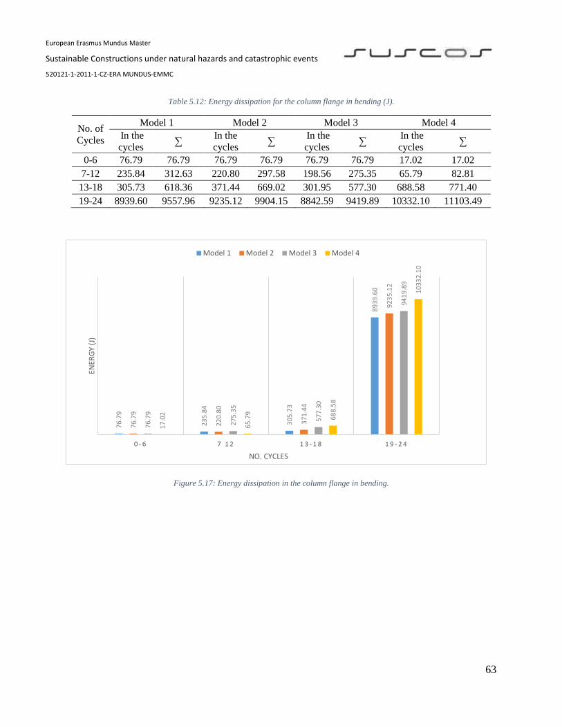
European Erasmus Mundus Master
Sustainable Constructions under natural hazards and catastrophic events
520121-1-2011-1-CZ-ERA MUNDUS-EMMC
63
Table 5.12: Energy dissipation for the column flange in bending (J).
No. of Cycles
Model 1 Model 2 Model 3 Model 4 In the cycles ∑ In the
cycles ∑ In the cycles ∑ In the
cycles ∑
0-6 76.79 76.79 76.79 76.79 76.79 76.79 17.02 17.02 7-12 235.84 312.63 220.80 297.58 198.56 275.35 65.79 82.81
13-18 305.73 618.36 371.44 669.02 301.95 577.30 688.58 771.40 19-24 8939.60 9557.96 9235.12 9904.15 8842.59 9419.89 10332.10 11103.49
Figure 5.17: Energy dissipation in the column flange in bending.
76.7
9
235.
84
305.
73
8939
.60
76.7
9
220.
80
371.
44
9235
.12
76.7
9
275.
35
577.
30
9419
.89
17.0
2
65.7
9
688.
58
1033
2.10
0 - 6 7 1 2 1 3 - 1 8 1 9 - 2 4
ENER
GY (J
)
NO. CYCLES
Model 1 Model 2 Model 3 Model 4

European Erasmus Mundus Master
Sustainable Constructions under natural hazards and catastrophic events
520121-1-2011-1-CZ-ERA MUNDUS-EMMC
64
Figure 5.18: Accumulative energy dissipation in the column flange in bending.
Table 5.13, Figure 5.19 and Figure 5.20 present the energy dissipation computed making use of
the normalized force vs deformation curves for the column flange in bending to remove the effect
of the strength of each model. Roughly, the same conclusion gathered from Table 5.12, Figure
5.17 and Figure 5.18 apply.
Table 5.13: Normalized energy dissipation for the column flange in bending
No. of Cycles
Model 1 Model 2 Model 3 Model 4 In the cycles ∑
In the cycles ∑
In the cycles ∑
In the cycles ∑
0-6 0.05 0.05 0.05 0.05 0.05 0.05 0.01 0.01 13-18 0.15 0.20 0.14 0.19 0.13 0.18 0.04 0.05 7 12 0.19 0.39 0.24 0.43 0.20 0.37 0.45 0.51
19-24 5.96 6.35 5.88 6.30 5.71 6.09 6.78 7.29
76.7
9
312.
63
618.
36
9557
.96
76.7
9
297.
58
669.
02
9904
.15
76.7
9
275.
35
577.
30
9419
.89
17.0
2
82.8
1 771.
40
1110
3.49
0 - 6 7 1 2 1 3 - 1 8 1 9 - 2 4
ENER
GY (J
)
NO. CYCLES
Model 1 Model 2 Model 3 Model 4

European Erasmus Mundus Master
Sustainable Constructions under natural hazards and catastrophic events
520121-1-2011-1-CZ-ERA MUNDUS-EMMC
65
Figure 5.19: Normalized energy dissipation for the column flange in bending
Figure 5.20: Accumulative normalized energy dissipation for the column flange in bending
0.05 0.15 0.19
5.96
0.05 0.14 0.24
5.88
0.05 0.13 0.20
5.71
0.01
0.04 0.
45
6.78
0 - 6 7 1 2 1 3 - 1 8 1 9 - 2 4
ENER
GY (J
)
NO. CYCLES
Model 1 Model 2 Model 3 Model 40.
05 0.20 0.
39
6.35
0.05 0.19 0.
43
6.30
0.05 0.18 0.
37
6.09
0.01 0.05
0.51
7.29
0 - 6 7 1 2 1 3 - 1 8 1 9 - 2 4
ENER
GY (J
)
NO. CYCLES
Model 1 Model 2 Model 3 Model 4

European Erasmus Mundus Master
Sustainable Constructions under natural hazards and catastrophic events
520121-1-2011-1-CZ-ERA MUNDUS-EMMC
66
5.3.2. Overall Model
Figure 5.21 shows the force-deformation relations for the FEM models where the force and
deformation were both gathered from RP3 in the FEM models. As already stated, these curves
characterize the behaviour of the entire tension region of the beam-to-column joint. i.e. the beam
flange in tension, the end plate in bending, the bolts in tension, the column flange in bending and
the column web in tension (with the stiffener).
Figure 5.21: Force-Displacement curves for cyclic loaded models
Figure 5.22 represent the normalized form of Force-Displacement curves obtained using a
procedure similar to the one used for the force vs deformation curves of the column flange in
bending.
-2000
-1500
-1000
-500
0
500
1000
1500
2000
0 1 2 3 4 5 6 7 8
Forc
e (k
N)
Displacement (mm)
Force vs Displacement
Model 1 Model 2 Model 3 Model 4

European Erasmus Mundus Master
Sustainable Constructions under natural hazards and catastrophic events
520121-1-2011-1-CZ-ERA MUNDUS-EMMC
67
Figure 5.22: Normalized Force-Displacement curves for cyclic loaded models
Both Figure 5.21 and Figure 5.22 show that the parameter β has a smaller influence in the overall
behaviour of the tension zone of the beam-to-column joint. This means that, e.g. the larger
deformation shown by the column flange in bending in Figure 5.15 are compensated with smaller
deformation in other parts of the tension region.
Table 5.14, Figure 5.23 and Figure 5.24 shows energy dissipation by the entire joint models. For
first 6 cyclic intervals, dissipation of energy is same in all models except model 4. It is also
perceived that β has significant relation with accumulation of energy of entire joint under cyclic
loading conditions, β is inversely proportional to energy dissipated by entire joint.
-1
-0.8
-0.6
-0.4
-0.2
0
0.2
0.4
0.6
0.8
1
0 1 2 3 4 5 6 7 8
F/Fm
ax
Displacement (mm)
Model 1 Model 2 Model 3 Model 4
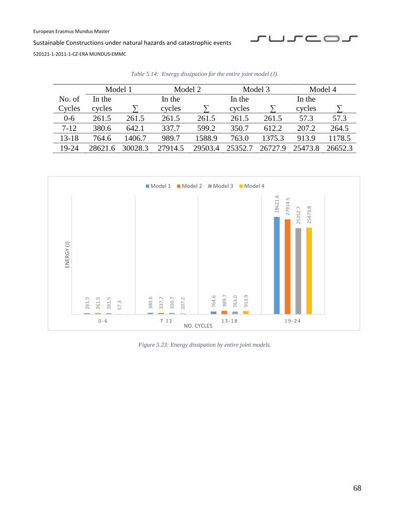
European Erasmus Mundus Master
Sustainable Constructions under natural hazards and catastrophic events
520121-1-2011-1-CZ-ERA MUNDUS-EMMC
68
Table 5.14: Energy dissipation for the entire joint model (J).
No. of Cycles
Model 1 Model 2 Model 3 Model 4 In the cycles ∑
In the cycles ∑
In the cycles ∑
In the cycles ∑
0-6 261.5 261.5 261.5 261.5 261.5 261.5 57.3 57.3 7-12 380.6 642.1 337.7 599.2 350.7 612.2 207.2 264.5 13-18 764.6 1406.7 989.7 1588.9 763.0 1375.3 913.9 1178.5 19-24 28621.6 30028.3 27914.5 29503.4 25352.7 26727.9 25473.8 26652.3
Figure 5.23: Energy dissipation by entire joint models.
261.
5
380.
6
764.
6
2862
1.6
261.
5
337.
7
989.
7
2791
4.5
261.
5
350.
7
763.
0
2535
2.7
57.3
207.
2
913.
9
2547
3.8
0 - 6 7 1 2 1 3 - 1 8 1 9 - 2 4
ENER
GY (J
)
NO. CYCLES
Model 1 Model 2 Model 3 Model 4

European Erasmus Mundus Master
Sustainable Constructions under natural hazards and catastrophic events
520121-1-2011-1-CZ-ERA MUNDUS-EMMC
69
Figure 5.24: Accumulative energy dissipation by entire joint models.
Comparison between dissipated energy in column flange and dissipated energy in complete joint
gives the awareness that column flange in bending plays an important role to dissipate the energy
of whole joint. 30–45 % energy is dissipated by column flange in bending component of joint
model and the remainder energy is dissipated by other components.
261.
5
642.
1
1406
.7
3002
8.3
261.
5
599.
2
1588
.9
2950
3.4
261.
5
612.
2
1375
.3
2672
7.9
57.3
264.
5
1178
.5
2665
2.3
0 - 6 7 1 2 1 3 - 1 8 1 9 - 2 4
ENER
GY (J
)
NO. CYCLES
Model 1 Model 2 Model 3 Model 4

European Erasmus Mundus Master
Sustainable Constructions under natural hazards and catastrophic events
520121-1-2011-1-CZ-ERA MUNDUS-EMMC
70
6. Conclusions and Recommendations for Future works
6.1. Conclusions
In this thesis, a FEM analysis was undertaken to assess the monotonic and cyclic behaviour of the
component stiffened column flange in bending in steel beam-to-column joints. A parametric
analysis was accomplished where a β parameter corresponding to the ratio of the strength of mode
1 and mode 2 of the equivalent T-Stub model suggested by EN1993-1-8 was changed in the range
[0.75, 1.25].
The analysis encountered convergence issues that prevented the collapse load being reached in the
monotonic and in the cyclic analysis.
The comparison of the collapse load of the stiffness column flange in bending according to the
equivalent T-Stub model and the behaviour of the FEM models that the collapse loads of the
equivalent T-Stub model are 25-35% higher than the elastic limits of the FEM models.
The FEM models of the stiffened column flange in bending showed that, along the first 24 cycles
of the loading protocol developed in the EQUALJOINTS project no strength degradation, no
stiffness degradation and no pinching effects are to be expected from this component.
The parametric analysis showed that the β parameter has a small influence in the behaviour of the
stiffened column flange in bending. It was found that higher β parameters may lead to larger energy
dissipation capacity but the trend is not clear.
Finally, the comparison of the energy dissipation in the column flange in bending and in the overall
model showed that the column flange in bending contributes to 30-45% dissipation of energy of
entire tension region of the joint.

European Erasmus Mundus Master
Sustainable Constructions under natural hazards and catastrophic events
520121-1-2011-1-CZ-ERA MUNDUS-EMMC
71
6.2. Recommendations for Future works
The bounds imposed by time requirements prevented a deeper analysis of the subjects accounted for in this thesis. For future works, it is believed that the following issues should be addressed:
• Use material models that take into account a combination of kinematic and isotropic flow
rules to simulate the cyclic behavior of the steel more accurately;
• Perform experimental tests to calibrate the numerical models;
• Solve the convergence issues encountered that prevented from reach the collapse of the
models;
• Assess the combined effect of the formation of modes 1 and 2 in end plate and column
flange;
• Assess the performance of the column flange in bending using a complete beam-column
joint model to evaluate the effect of the redistribution of internal forces in the impact of the
response of this component and to assess its actual demand;

European Erasmus Mundus Master
Sustainable Constructions under natural hazards and catastrophic events
520121-1-2011-1-CZ-ERA MUNDUS-EMMC
72
7. References
[1] CEN. Euro code 3: design of steel structures — part 1-1: general rules and rules for
buildings. CEN, Brussels: European Committee for Standardization; 2005.
[2] CEN. Euro code 3: design of steel structures — part 1–8: design of joints. CEN, Brussels:
European Committee for Standardization; 2005.
[3] A. Tsitos, A. Elghazouli, M. D’Aniello, S. Costanzo, R Landolfo, A. Stratan, G. Sabău, Dan
Dubina, F. Gentili, C. Rebelo and L. S.s da Silva. Selection of loading protocols Deliverable d-p3-
1. Rev. 01. February 2016
[4] L. Massimo, Rizzano G, S. Aldina, Simões da Silva L, Experimental analysis and mechanical
modelling of T-stubs with four bolts per row. Journal of Construction Steel Research 101 (2014)
158-174.
[5] Faella C, Montuori R, Piluso V, Rizzano G. Failure mode control: economy of semi rigid
frames. Proceedings of the XI European Conference on Earthquake Engineering. Paris; 1998.
[6] Faella C, Piluso V, Rizzano G. Cyclic behavior of bolted joint components Journal of
Construction Steel Research 1998;46(1-3) [p. paper number 129].
[7] Ciro Faella, Vincenzo Piluso, Gianvittorio Rizzano. Structural Steel Semi Rigid Connections:
Theory, Design, and Software, WF. CHEN, CRC Press
[8] Piluso V, Rizzano G. Experimental analysis and modelling of bolted T-stub under cyclic loads.
Journal of Construction Steel Research 64 (2008) 655-669.
[9] Swanson JA, Leon RT. Bolted steel connections: tests on T-stub components. Journal of
Structural Engineering, ASCE 2000;126(1):50–6.
[10] Jaspart J-P, Weynand K. Design of joints in steel and composite structures, published by
ECCS – European convention constructional steelwork; 2016.
[11] Hugo Renato Gonçalves da Silva Augusto. Characterization of the behaviour of partial-
strength joints under cyclic and seismic loading conditions. PhD thesis, Coimbra, Portugal, 2017.

European Erasmus Mundus Master
Sustainable Constructions under natural hazards and catastrophic events
520121-1-2011-1-CZ-ERA MUNDUS-EMMC
73
[12] Zeotemeijer P. A design method for the tension side of statically loaded, bolted beam-to-
column connections. Heron Vol. 20 1974 no.1.
[13] J.P. Jaspart, J.F. Demonceau. Structural joints with more complex geometry and loading. Steel
Connection Design – SUSCOS 1C2 Course – September 2016
[14] Dieter Declerck. Comparison between the Euro code methodology and a finite element model:
the equivalent T-Stub method. MSc thesis, Gent, Belgium, 2016-2017
[15] Muhammad Asghar Bhatti. Fundamental finite element analysis and applications. John Wiley
& Sons Inc. 2005.
[16] Simulia, “Getting Started with ABAQUS: Interactive Edition,” Get. Started with ABAQUS
Interact. Ed., p. 4.50-4.54, 2012.
[17] “Recommended testing procedure for assessing the behaviour of structural steel elements
under cyclic loads”, ECCS-Technical Committee 1 - Structural safety and loadings technical
working group 1.3 - Seismic design. First edition.