HAL Id: hal-00679118https://hal.archives-ouvertes.fr/hal-00679118

Submitted on 14 Mar 2012

HAL is a multi-disciplinary open accessarchive for the deposit and dissemination of sci-entific research documents, whether they are pub-lished or not. The documents may come fromteaching and research institutions in France orabroad, or from public or private research centers.

L’archive ouverte pluridisciplinaire HAL, estdestinée au dépôt et à la diffusion de documentsscientifiques de niveau recherche, publiés ou non,émanant des établissements d’enseignement et derecherche français ou étrangers, des laboratoirespublics ou privés.

Feedrate interpolation with axis jerk constraints on5-axis NURBS and G1 tool path

Xavier Beudaert, Sylvain Lavernhe, Christophe Tournier

To cite this version:Xavier Beudaert, Sylvain Lavernhe, Christophe Tournier. Feedrate interpolation with axis jerk con-straints on 5-axis NURBS and G1 tool path. International Journal of Machine Tools & Manufacture,2012, pp.10. <10.1016/j.ijmachtools.2012.02.005>. <hal-00679118>

Feedrate interpolation with axis jerk constraints on 5-axis NURBS and G1 toolpath

Xavier Beudaert, Sylvain Lavernhe, Christophe Tournier∗

LURPA, ENS Cachan, Universite Paris Sud 1161 av du pdt Wilson, 94235 Cachan, France

name@lurpa.ens-cachan.fr

Abstract

A key role of the CNC is to perform the feedrate interpolation which consists in generating the setpoints sent to eachaxis of a machine tool based on a NC program. In high speed machining, the feedrate is limited by the velocity,acceleration and jerk of each axis of the machine tool.The algorithm presented in this paper aims to obtain an optimized feedrate profile which makes best use of thekinematical characteristics of the machine. This minimum time feedrate profile is computed by intersecting all theconstraints due to the drives in an iterative algorithm. It is worth noting that both tangential jerk and axis jerk are takeninto consideration. The proposed VPOp (Velocity Profile Optimization) method is universal and can be applied to anyarticulated mechanical structure as it is demonstrated in the examples. Moreover the algorithm has been implementedfor various formats: linear interpolation (G1) and NURBS interpolation in 3 and 5-axis. The effectiveness of thealgorithm is demonstrated thanks to a comparison with an industrial CNC and can be freely tested using the VPOpsoftware which is available on the internet http://webserv.lurpa.ens-cachan.fr/geo3d/premium/vpop.

Keywords: 5-axis machining, feedrate, jerk, drive constraint, velocity planning, CNC

Nomenclature

L the length of the tool path (m)s path displacement (m) s ∈ [0, L]s feedrate (m/s)s tangential acceleration (m/s2)...s tangential jerk (m/s3)Fpr programmed feedrate (m/min)Atan maximum tangential acceleration (m/s2)Jtan maximum tangential jerk (m/s3)

The following notation are illustrated on a 5-axis XYZAC structure.q = [X(s) Y(s) Z(s) A(s) C(s)]T axes position (m or rad)q = [X(s) Y(s) Z(s) A(s) C(s)]T axes velocity (m/s or rad/s)q = [X(s) Y(s) Z(s) A(s) C(s)]T axes acceleration (m/s2 or rad/s2)...q = [

...X(s)

...Y (s)

...Z (s)

...A(s)

...C(s)]T axes jerk (m/s3 or rad/s3)

∗Corresponding author

Preprint submitted to International Journal of Machine Tools and Manufacture March 14, 2012

qs = [Xs(s) Ys(s) Zs(s) As(s) Cs(s)]T

qss = [Xss(s) Yss(s) Zss(s) Ass(s) Css(s)]T

qsss = [Xsss(s) Ysss(s) Zsss(s) Asss(s) Csss(s)]T

first, second and third derivatives of the 5-axis positions with respect to the path displacement s

i i = 1..5 for the X, Y, Z, A, C axes of the machine toolN number of discretized calculation pointsj j = 1..N discretized value along the paths j jth discretized point along s

Vmax = [vmax,x vmax,y vmax,z vmax,a vmax,c]T axes velocity limits (m/s or rad/s)Amax = [amax,x amax,y amax,z amax,a amax,c]T axes acceleration limits (m/s2 or rad/s2)Jmax = [ jmax,x jmax,y jmax,z jmax,a jmax,c]T axes jerk limits (m/s3 or rad/s3)

2

1. Introduction

This paper deals with the interpolation which is realized by the Computer Numerical Control (CNC). Indeed,starting from a NC program the CNC generates the setpoints for the machine’s axes. So the input is a reference toolpath with a programmed feedrate and the output is a sequence of axis setpoints which have to produce a smoothmovement. As previously shown in [1], there are three main approaches to solve the problem of interpolation: (a)Time-parameterization of geometric paths (decoupled approach), (b) Combined path-planning and time parameteri-zation (combined approach), (c) Reactive and hybrid methods. The reactive and hybrid methods are used for exampleto drive a mobile robot which must adapt to its unknown environment. This method is not usefull in this context asfor machining operations the environment is known in advance. The combined approach is mainly used for roboticmanipulators as it is well suited for trajectory without strong constraints on the contour error. Indeed, for a point topoint movement, it is possible to infer the fastest tool path by planning each joint movement independently. With thismethod the kinematical characteristics of the joint impose the geometryof the tool path. For machining operations,the main goal is to follow precisely a given geometric path, for that reason, the decoupled approach is preferred. Thisapproach consists in decoupling the geometry from the temporal evolution law. So the first part of the job is to createa ”satisfying” geometry and then the feedrate interpolation is performed on that fixed geometry to generate the axissetpoints.

Computer-aided manufacturing (CAM) software generates the tool path first and then the CNC of the machinetool has to create the feedrate profile to follow this given geometry respecting the drive constraints. Industrially, Gcode is generally employed to describe the tool path. However, this description consists of segments connected withtangential discontinuities. So the discontinuities have to be rounded in order to be able to go through with non nullfeedrate. That is why the first task of the numerical controller is to modify the geometry in order to round off thediscontinuities. Indeed, the CNC is using the contour tolerance to go through the transitions between G1 blocks witha non null feedrate. The best solution is to use a native mathematical description such as NURBS (Non-UniformRational Basis Splines) but unfortunately it is hardly ever used industrially. The polynomial formalism allows havinga continuous path which will be interpolated by the CNC without any geometrical modification as opposed to the G1description. To overcome this problem, the industrial CNCs offer the possibility to use real time compressors to createa spline with a set of G1 points (see CompCad/CompCurv in [2]).

Feedrate interpolation was first studied in robotics. For example, the problem of transition between segmentswas addressed in [3]. More recently, a corner rounding method mixing the geometry and the time parametrization isproposed in [4] but it requires some assumptions especially for the feedrate at the entry and exit of the discontinuity.A method based on tool path / feedrate modification on the vicinity of the discontinuity was proposed in [5]. As itis mentioned above, it is preferable to decouple the geometry from the time parametrization. In tool path generation,[6] proposed a solution with a cubic B-Spline with six control points to round 3-axis tool paths. A good solution for3-axis corner rounding is given in the Siemens patent [7] where polynomial splines are used to round the corners.

Once the geometrical treatment of the tool path is carried out, the feedrate planning has to be performed. The aimis to find an optimized feedrate profile which makes best use of the kinematical characteristics of the machine whilefollowing the given geometry.

Feedrate planning is a known issue and can be solved using different methods and taking into account differentconstraints. In robotics, Bobrow et al. [8] and Shin and McKay [9] proposed a two pass iterative algorithm basedon the constraints intersection principle. The idea is to start from the beginning of the tool path and to go as fastas possible even if some constraints are not respected. Then in the reverse pass, the procedure is repeated with theadditional constraint that the feedrate is lower than in the forward pass. Finally, a corrective algorithm is appliedto connect both passes with acceleration constraints. This two pass algorithm was reused and improved. Rentonand Elbestawi [10] worked on the velocity and acceleration limits determination. Timar et al. [11] used polynomialparametric curves on which they could obtained a closed form solution for the feedrate planning problem with axisacceleration constraints. Dong and Stori [12] tried to prove the optimality of the two pass algorithm. All the previouslycited articles took velocity and acceleration constraints of the drives. But it is well known that jerk is an importantparameter which should be considered as well. Indeed in many high speed milling operations jerk is the parameterwhich limits the feedrate variations.

The effect of jerk limitation on the mechanical structure was studied in detail by Barre et al. [13]. It is clear that

3

jerk has to be limited to reduce the frequency content of the trajectory and to avoid exciting the natural modes of thestructure. However, several articles are dealing with the tangential jerk only (third derivative with respect to the timeof the tool/workpiece movement). This can be interesting for manipulators but to avoid vibrations of a machine toolstructure, each axis jerk (third derivative with respect to the time of the axis movement) limit has to be considered too.Liu et al. [14] modified the feedrate profile to take into account the jerk and the natural frequencies of the machinetool. This method should be applied carefully to control the contour error generated.

Dong et al. [15] introduced jerk constraint to the two pass iterative algorithm. At first sight, it does not seemchallenging to add another constraint. But in fact, it is really hard to connect the forward and the backward passrespecting jerk constraints. Indeed a lot of points have to be modified and for complex shapes the switching points canbe too close and the whole feedrate profile has to be modified by a corrective algorithm. The other main method torealize the feedrate planning with jerk constraints is to use a predefined profile as presented in Erkorkmaz and Altintas[16]. The objective of this method is to generate a sequence of predefined profiles which respects the constraints.This solution was also used and improved in many other works, e.g. [17–20]. Olabi et al. [21] applied the predefinedprofile to an industrial 6-axis machining robot. Lin et al. [22] introduced a cascade structure with a feedforwardcontroller and the contour error in their interpolator. But the main problem is that the constraint on the predefinedprofile limits only the tangential derivatives. In practice each axis has its own limitations; furthermore with linear androtary drives it is impossible to make the link between tangential jerk and axis jerk due to the non linear kinematicaltransformation.

In the literature, few works are can be found concerning multi-axis machining with linear and rotary axes. Themethods with predefined feedrate profile cannot be applied to this kind of machine as the kinematical transformationbetween the cartesian space and the joint space is non-linear. Thus the tangential limits have to be really conservativeto make sure that the axis kinematical limits are not exceeded.

On 5-axis machining with axis jerk constraints, Lavernhe et al. [23, 24] presented a predictive model of kine-matical performance using an iterative time inverse method. This method is suited for G1 tool path but it is difficultto apply it to NURBS tool path. Sencer et al. [25] represented the feedrate profile with a cubic B-Spline which isiteratively modulated to minimize the machining time. This method is suited for NURBS tool path but it is difficult toapply it to G1 format.

The goal of this paper is to propose a unified feedrate planning solution for any machine tool structure with bothjerk axis constraints and tangential jerk constraint along the tool path. A decoupled approach is used to separate thegeometrical problem from the temporal interpolation problem. A one way interpolation method assuring the respectof all the constraints at each time step is used. This time discretization allows avoiding some further reinterpolationproblems. The use of a look ahead based on the geometrical analysis of the tool path helps the interpolation in sharpzones. Both linear (G1) and polynomial (NURBS) tool path are handled in this paper. Furthermore, the mathematicalformulation used here allows treating both linear and rotary axes in the same way. Hence, the algorithm is suitable forserial and parallel kinematic machine.

The plan for the remainder of this paper is as follows. Section 2 details the feedrate planning which aims to findthe velocity profile which makes best use of the kinematical characteristics of the machine tool. Experiments andsimulations are carried out in Section 3 to demonstrate the efficiency of the proposed method. Finally, the paper isconcluded in Section 4.

2. Feedrate planning algorithm

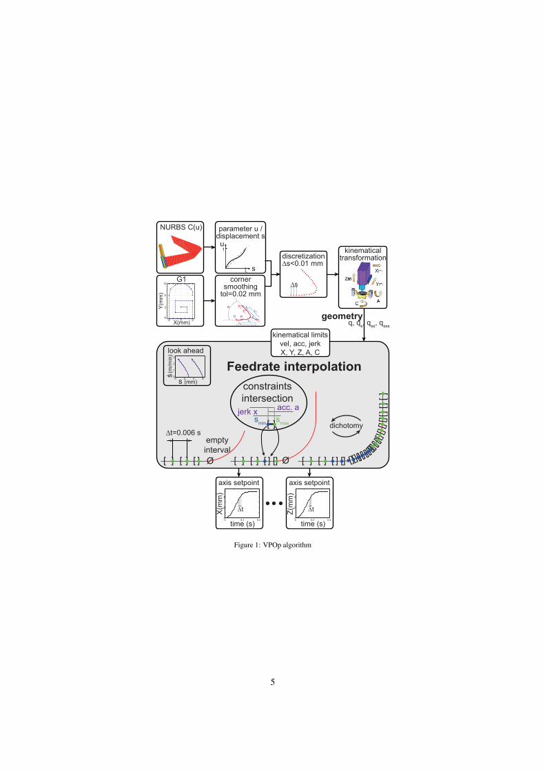
Fig. 1 shows the whole procedure. First the geometrical work is carried out. Then the kinematical transformationis used to obtain the joint movements. After that, the temporal interpolation is performed along this fixed geometryusing a constraint intersection principle and a dichotomy which will be detailed. Finally the output is the sampled axissetpoints respecting velocity, acceleration and jerk constraints of each drive and of the tangential movement.

2.1. Mathematical formalism and drive constraintsUsing the formula for the derivative of the composition of two functions (Eq.1), it is possible to express the velocity

of the drives q as a function of the geometry qs multiplied by a function of the motion s. Therefore, the motion is

4

emptyinterval

G1 cornersmoothing

tol=0.02 mm

Feedrate interpolation

geometry

∆t=0.006 s

parameter u /displacement s

discretization∆s<0.01 mm

kinematicaltransformation

dichotomy

u

s

1

L

axis setpoint

q, qs, qss, qsss

NURBS C(u)

axis setpoint

0 0.2 0.40

2

4

Z(m

m)

time (s)

∆t0 0.2 0.40

2

4

X(m

m)

time (s)

∆t

[ ] [ ] [ ] Ø [ ] [ ] [ ] Ø[] [ ] [ ] [ ] [] [][][]][][][][]

[][][][]

[][][

][][

][]constraints

intersectionjerk x acc. a

smin smax[ ]

P0

L2

P2

P1

P3

P4

L1L2

L1

α

ε

∆s

-6 0 6-6

0

6

12

X(mm)

Y(m

m)

look ahead

0 2 4 60

1

2

3

s (mm)

(m/m

in)

s

kinematical limitsvel, acc, jerkX, Y, Z, A, C

Figure 1: VPOp algorithm

5

decoupled from the geometry. One can note that this formula is valid for linear and rotary axes. The acceleration qand jerk

...q of the drives are obtained identically in Eq.2 and 3.

q =dqdt

=dqds

dsdt

= qs s (1)

q = qss s2 + qs s (2)

...q = qsss s3 + 3qss s s + qs...s (3)

qs, qss, qsss are the geometrical derivatives with respect to the displacement s along the tool path. They are knownas soon as the geometrical treatment of the tool path is realized. Because of the physical realization of the drives(motors, driving system, machine tool structure ...) the velocity, acceleration and jerk of each individual drive have tobe limited. The jerk limitation is important to reduce the vibration due to the dominating vibratory mode of the axes.For example, for a 5-axis machine tool, the velocity constraints for each discretized point j along the tool path arepresented in Eq.4.

−

vmax,x

vmax,y

vmax,z

vmax,a

vmax,c

≤

X js

Y js

Z js

A js

C js

s j ≤

vmax,x

vmax,y

vmax,z

vmax,a

vmax,c

(4)

All the constraints are set to be symmetrical as it is commonly used in the machine tool characteristics. Then thefollowing set of inequations is obtained respectively for the velocity, acceleration and jerk constraints. The notation | |stands for the absolute value of each scalar term.

|q ji | ≤ Vmax,i ; |q j

i | ≤ Amax,i ; |...q j

i | ≤ Jmax,i (5)

It is possible to obtain in a close form an approximation of the upper limit of the feedrate. This limit is a goodevaluation of the feedrate which can be used to optimize the tool path as in [26] but it is not sufficient to control amachine tool. Indeed, the need is to find a velocity profile which respects all the kinematical constraints without anyapproximation.

2.2. Discretization and principle of the algorithmFor a discretized algorithm, two discretizations are conceivable: a geometrical discretization in ∆u (constant curve

parameter step) or in ∆s (constant path displacement step) as in [12, 15] for example or a discretization in time ∆t(constant time step). The problem with the discretization in ∆s is that eventually the setpoints have to be send to thecontroller with a fixed frequency so a reinterpolation is needed. At really low feedrate a small ∆s increment is neededto be closed to the desired command frequency. Therefore at high feedrate many useless points will be computed.Moreover, with a fixed ∆s the evaluation of the jerk will be really rough. The quintic spline interpolation presented in[16] will also have this problem to reinterpolate the points computed in ∆s so it cannot ensure that the jerk limitationwill not be exceeded. That is why a constant time step has been chosen for the VPOp algorithm presented here. Hence,the velocity, acceleration and jerk are computed as in the Eq. 6.

s j+1 =s j+1 − s j

∆t, s j+1 =

s j+1 − s j

∆t,

...s j+1 =

s j+1 − s j

∆t(6)

The aim of the algorithm is to calculate the next reachable point with a fixed ∆t knowing all the characteristics onthe previous points. This is done by intersecting all the constraints as proposed in [8, 9]. Using the discretization, eachconstraint can be reduced to a polynomial inequation Eq.7-9. The unknown parameter is s j+1, and f are functionsof the geometrical derivatives. Solving the inequation, an interval over which the constraint is verified is obtained.Finally, as shown in Fig.2, the intersection of all these intervals gives the solution interval [smin, smax] into which allthe constraints are respected for this step. It is possible to have a solution which is a simple interval or a union of

6

OUTPUT:

INPUT: sj, sj-1, sj-2, geometry, kinematical limits, Δt, Fpr

tangential jerk

tangential acceleration

tangential feedrate

axis jerk

axis acceleration

axis velocity

0 ≤ sj+1 ≤ Fpr

−Atan ≤ sj+1 ≤ A tan

−Jtan ≤...s j+1 ≤ Jtan

−Vmax,i ≤ qj+1i ≤ Vmax,i

−Amax,i ≤ qj+1i ≤ Amax,i

−Jmax,i ≤...q j+1

i ≤ Jmax,i

sj+1 [smin,smaxЄ [

0 Fpr

[ ]

Figure 2: Constraints intersection principle.

distinct intervals [smin, s2] ∪ [s3, smax]. In this case, the minimum and maximum allowable solutions smin and smax arekept. This interval can also be empty, for example when the feedrate is too high at the entrance of a sharp curvaturearea. In this case, it is necessary to go few steps back to reduce the feedrate.

−Vmax,i ≤ q j+1s,i ·

s j+1 − s j

∆t≤ Vmax,i (7)

−Amax,i ≤ s2j+1 · fA2 + s j+1 · fA1 + fA0 ≤ Amax,i (8)

−Jmax,i ≤ s3j+1 · fJ3 + s2

j+1 · fJ2 + s j+1 · fJ1 + fJ0 ≤ Jmax,i (9)

The functions fA0, fA1, fA2 used in the Eq. 8 are detailed below Eq.10-12. Those equations are obtained usingEq. 1-3 and Eq. 6. The functions fJ0, fJ1, fJ2, fJ3 can be obtained in the same way. Those functions depend on thepositions s j, s j−1, s j−2 calculated in the previous iterations and on the geometrical derivative at the point j + 1 whichwill be approximated as explained in Section 2.6.

fA2 =q j+1

ss,i

∆t2 (10)

fA1 =1

∆t2 ·(q j+1

s,i − q j+1ss,i · 2s j

)(11)

fA0 =1

∆t2 ·(q j+1

ss,i · s2j + q j+1

s,i

(s j−1 − 2s j

))(12)

2.3. Detailed explanation of the algorithmThe iteration principle to find the correct sequence of smin, smax is briefly described in Fig. 1. In order to show

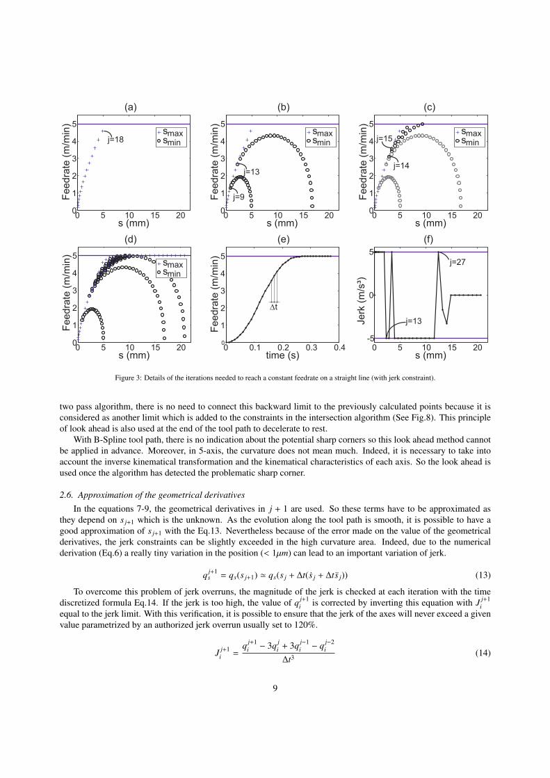
explicitly how the algorithm is working, it has been applied on a really simple example. The tool path is a straightline and the aim is to reach the programmed feedrate starting from rest. The feedrate will be limited only by theprogrammed feedrate and the jerk of the axis which are respectively 5m/min and 5m/s3. The Fig.3 shows eachcalculated point. On Fig.3.a, one can see that the algorithm starts going as fast as possible until a point with no

7

solution (empty intersection) is reached after j = 18. Indeed, it is impossible to stay under the programmed feedratewhile respecting the acceleration and jerk constraints.

That means that the sequence used on the previous points was wrong. To find the switching point where smin hasto be chosen instead of smax a dichotomy is used. The idea is to say that if it is possible to find a sequence whichallows reaching s = 0, it will be possible to find a sequence which allows reaching the programmed feedrate withoutexceeding it. To reach s = 0, it is necessary to decelerate as much as possible so a sequence using always smin is tried.

The first point from where s = 0 can be reached is find with a dichotomy. In Fig.3.b smin is taken from j = 9 ands = 0 is reached so it is possible to go further. With j = 13, s = 0 is reached again. So on Fig.3.c j = 15 is tested, nosolution is found. The last iteration of the dichotomy is in j = 14, here again s = 0 cannot be reached. So it is sure thats13 = smin has to be chosen to be able to obtain a solution. Once the dichotomy is finished, the algorithm tries againto go as fast as possible taking smax at each step. Finally, Fig.3.d shows all the points which have been calculated toreach the constant feedrate while respecting the jerk constraint. One can see on Fig. 3.e that the feedrate profile isreally smooth. Fig.3.f demonstrates that the jerk limit is respected, after the point j = 27 the limiting parameter isthe programmed feedrate. The sequence of jerk presents peaks so it is not the one expected mathematically. But adiscretized algorithm will always create this kind of solution as the optimal solution is not contained on the set of thediscretized solutions. A better solution could be obtained by choosing points in the middle of the [smin smax] intervalat the expense of complexity and computation load.

The same kind of problems will be encountered when a sharp corner is reached with a high feedrate as in the firsttrial of Fig. 1. So using the same technique of dichotomy, the first point from where it is possible to reach s = 0 hasto be found. If it is possible to find a sequence to reach s = 0, it will be possible to find a sequence which respectsall the constraints on any geometry (including any potential upcoming sharp corner). Here, it is assumed that if it ispossible to reach s = 0, it will always be possible to go further. In reality, the algorithm sometimes needs to go backeven more because the deceleration is too high to be able to stop at s = 0 with s = 0.

2.4. Algorithm

The detailed algorithm is written below:Prepare the geometry of the tool pathApply the look ahead for each G1 transition and at the end of the tool pathwhile the end of the tool path is not reached do

Compute the intersection of the intervalsif intersection is empty then

while the end of the dichotomy is not reached doUse a dichotomy to find the point j where s j = smin has to be chosen. Indeed as there is no solution, thefirst point from where it is possible to reach s = 0 taking smin for each step has to be found. To speed up thealgorithm, this research is realized with a dichotomy.

end whileelse

s j+1 = smax

end ifend while

There is no attempt to demonstrate the optimality of the solution as it depends on the time step ∆t and on thescheme chosen to compute the discrete derivatives. The proposed algorithm is not designed to be optimal but it isrobust and it gives a solution which is really close to the mathematical optimal solution.

2.5. Look ahead

With a G1 tool path, it is known in advance that the feedrate will be minimum at the discontinuities. So a lookahead strategy is used in order to reduce the number of iterations. The look ahead consists in calculating the necessaryfeedrate reduction to approach a sharp corner. Starting from the middle of each transition with zero acceleration andjerk, this look ahead uses the algorithm previously described but applied in the backward direction. As opposed to a

8

0 5 10 15 200

1

2

3

4

5

Feed

rate

(m/m

in)

s (mm)0 5 10 15 200

1

2

3

4

5

Feed

rate

(m/m

in)

s (mm)0 5 10 15 200

1

2

3

4

5

Feed

rate

(m/m

in)

s (mm)

0 0.1 0.2 0.3 0.40

1

2

3

4

5

Feed

rate

(m/m

in)

time (s)0 5 10 15 20

-5

0

5

Jerk

(m/s

³)s (mm)

0 5 10 15 200

1

2

3

4

5

s (mm)

Feed

rate

(m/m

in)

(a)

(d)

(b)

(e)

(c)

(f)

smaxsmin

smaxsmin

smaxsmin

smaxsminj=18

j=9

j=13

j=15

j=14

j=13

∆t

j=27

Figure 3: Details of the iterations needed to reach a constant feedrate on a straight line (with jerk constraint).

two pass algorithm, there is no need to connect this backward limit to the previously calculated points because it isconsidered as another limit which is added to the constraints in the intersection algorithm (See Fig.8). This principleof look ahead is also used at the end of the tool path to decelerate to rest.

With B-Spline tool path, there is no indication about the potential sharp corners so this look ahead method cannotbe applied in advance. Moreover, in 5-axis, the curvature does not mean much. Indeed, it is necessary to take intoaccount the inverse kinematical transformation and the kinematical characteristics of each axis. So the look ahead isused once the algorithm has detected the problematic sharp corner.

2.6. Approximation of the geometrical derivatives

In the equations 7-9, the geometrical derivatives in j + 1 are used. So these terms have to be approximated asthey depend on s j+1 which is the unknown. As the evolution along the tool path is smooth, it is possible to have agood approximation of s j+1 with the Eq.13. Nevertheless because of the error made on the value of the geometricalderivatives, the jerk constraints can be slightly exceeded in the high curvature area. Indeed, due to the numericalderivation (Eq.6) a really tiny variation in the position (< 1µm) can lead to an important variation of jerk.

q j+1s = qs(s j+1) ' qs(s j + ∆t(s j + ∆ts j)) (13)

To overcome this problem of jerk overruns, the magnitude of the jerk is checked at each iteration with the timediscretized formula Eq.14. If the jerk is too high, the value of q j+1

i is corrected by inverting this equation with J j+1i

equal to the jerk limit. With this verification, it is possible to ensure that the jerk of the axes will never exceed a givenvalue parametrized by an authorized jerk overrun usually set to 120%.

J j+1i =

q j+1i − 3q j

i + 3q j−1i − q j−2

i

∆t3 (14)

9

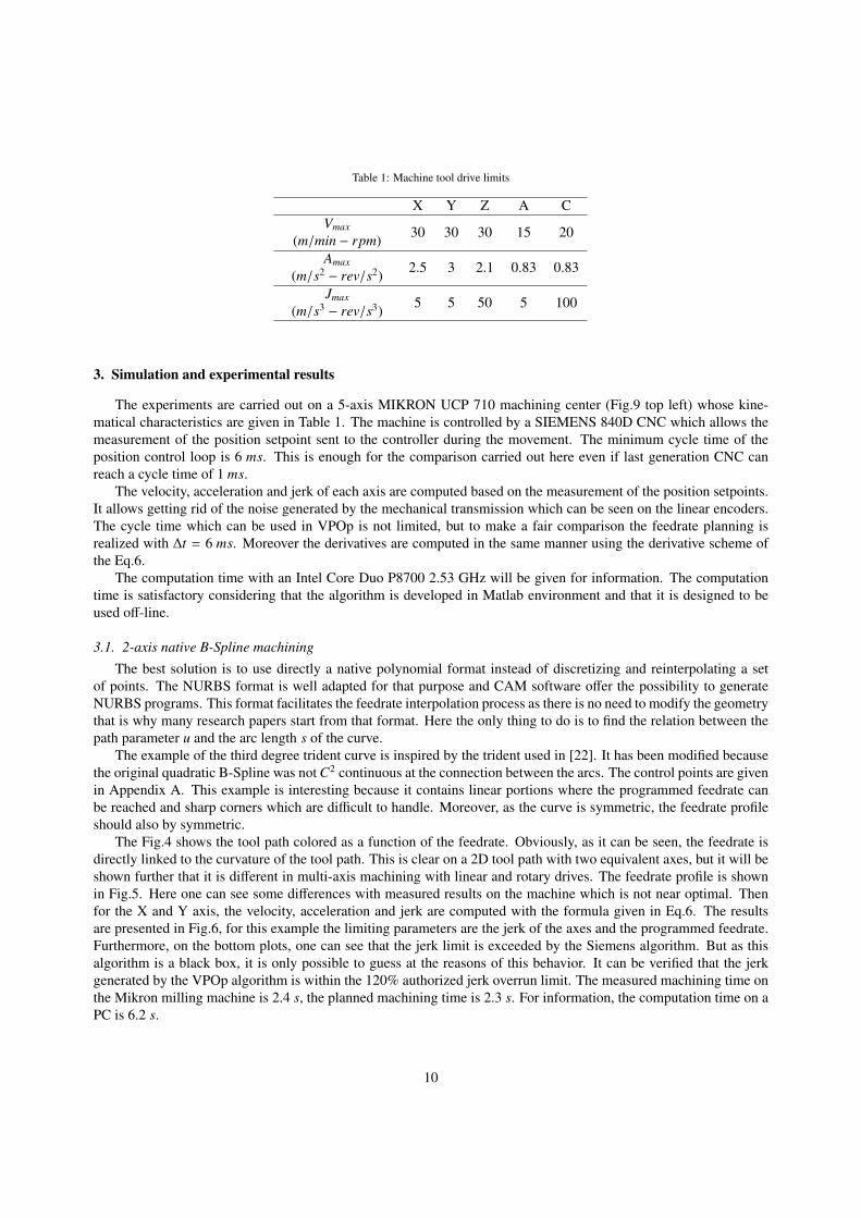
Table 1: Machine tool drive limits

X Y Z A CVmax

(m/min − rpm) 30 30 30 15 20

Amax

(m/s2 − rev/s2) 2.5 3 2.1 0.83 0.83

Jmax

(m/s3 − rev/s3) 5 5 50 5 100

3. Simulation and experimental results

The experiments are carried out on a 5-axis MIKRON UCP 710 machining center (Fig.9 top left) whose kine-matical characteristics are given in Table 1. The machine is controlled by a SIEMENS 840D CNC which allows themeasurement of the position setpoint sent to the controller during the movement. The minimum cycle time of theposition control loop is 6 ms. This is enough for the comparison carried out here even if last generation CNC canreach a cycle time of 1 ms.

The velocity, acceleration and jerk of each axis are computed based on the measurement of the position setpoints.It allows getting rid of the noise generated by the mechanical transmission which can be seen on the linear encoders.The cycle time which can be used in VPOp is not limited, but to make a fair comparison the feedrate planning isrealized with ∆t = 6 ms. Moreover the derivatives are computed in the same manner using the derivative scheme ofthe Eq.6.

The computation time with an Intel Core Duo P8700 2.53 GHz will be given for information. The computationtime is satisfactory considering that the algorithm is developed in Matlab environment and that it is designed to beused off-line.

3.1. 2-axis native B-Spline machining

The best solution is to use directly a native polynomial format instead of discretizing and reinterpolating a setof points. The NURBS format is well adapted for that purpose and CAM software offer the possibility to generateNURBS programs. This format facilitates the feedrate interpolation process as there is no need to modify the geometrythat is why many research papers start from that format. Here the only thing to do is to find the relation between thepath parameter u and the arc length s of the curve.

The example of the third degree trident curve is inspired by the trident used in [22]. It has been modified becausethe original quadratic B-Spline was not C2 continuous at the connection between the arcs. The control points are givenin Appendix A. This example is interesting because it contains linear portions where the programmed feedrate canbe reached and sharp corners which are difficult to handle. Moreover, as the curve is symmetric, the feedrate profileshould also by symmetric.

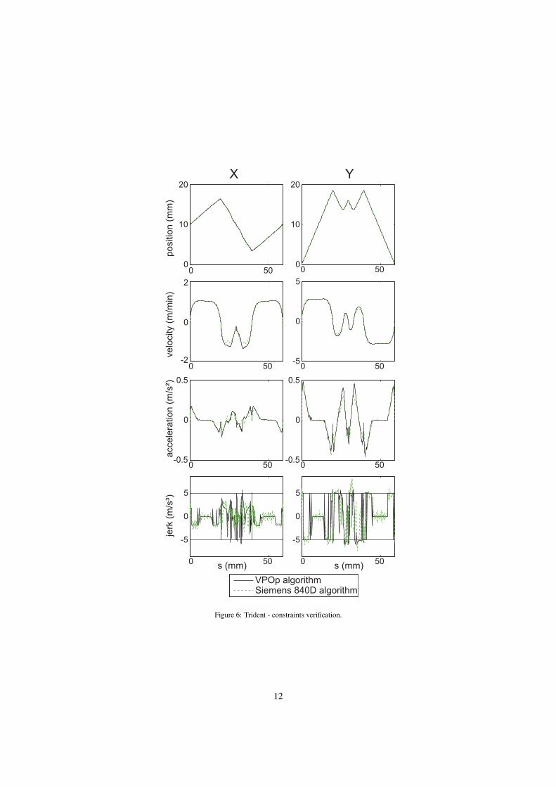
The Fig.4 shows the tool path colored as a function of the feedrate. Obviously, as it can be seen, the feedrate isdirectly linked to the curvature of the tool path. This is clear on a 2D tool path with two equivalent axes, but it will beshown further that it is different in multi-axis machining with linear and rotary drives. The feedrate profile is shownin Fig.5. Here one can see some differences with measured results on the machine which is not near optimal. Thenfor the X and Y axis, the velocity, acceleration and jerk are computed with the formula given in Eq.6. The resultsare presented in Fig.6, for this example the limiting parameters are the jerk of the axes and the programmed feedrate.Furthermore, on the bottom plots, one can see that the jerk limit is exceeded by the Siemens algorithm. But as thisalgorithm is a black box, it is only possible to guess at the reasons of this behavior. It can be verified that the jerkgenerated by the VPOp algorithm is within the 120% authorized jerk overrun limit. The measured machining time onthe Mikron milling machine is 2.4 s, the planned machining time is 2.3 s. For information, the computation time on aPC is 6.2 s.

10

0 5 10 15 200

5

10

15

20

25

X(mm)

Y(m

m)

feedratem/min

0

0.5

1

1.5

2

2.5

3control points

O

A

BC

D

E

Figure 4: Trident - tool path.

0 10 20 30 40 500

0.5

1

1.5

2

2.5

3

Displacement s (mm)

Feed

rate

(m/m

in)

VPOp algorithmSiemens 840D algorithm

A

B

C

D

EO O

Figure 5: Trident - feedrate.

11

posi

tion

(mm

)

0 500

10

20X

0 500

10

20Y

velo

city

(m/m

in)

0 50-2

0

2

0 50-5

0

5

acce

lera

tion

(m/s

²)

0 50-0.5

0

0.5

0 50-0.5

0

0.5

jerk

(m/s

³)

0 50

-5

0

5

0 50

-5

0

5

s (mm) s (mm)VPOp algorithmSiemens 840D algorithm

Figure 6: Trident - constraints verification.

12

-0.4 0 0.4

11.8

11.9

12

12.1

X(mm)

Y(m

m)

-10 -8-6

-4

-2

0

2

4

6

8

10

12

Y(m

m)

-6 -4 -2 0 2 4 6 8 10X(mm)

π/6 π/12

A B

CD

E F

GH

I

J

KL M

N

O

P

Q

R

Feedrate(m/min)

0

3

1.5

2

2.5

1

0.5

L

ε=0.02 mm

0 10 20 30 40 50 60 700

0.5

1

1.5

2

2.5

3

3.5

4

Displacement s (mm)Fe

edra

te (m

/min

)

VPOp algorithmSiemens 840D algorithm

AB C

D E F G H

I

J K L

N

O

P

Q

R

jerk

(m/s

3 )

0 50-5

0

5

0 50-5

0

5

s (mm) s (mm)

X Y

(b)

(c)

(a)

Figure 7: (a) lock tool path, (b) feedrate profile, (c) jerk constraints verification

3.2. 2-axis G1 machining

The geometrical treatment and the feedrate planning of a G1 tool path are presented on the lock tool path Fig.7(a).This example contains short segments upon which the programmed feedrate cannot be reached and a discretizedarc of circle which emphasized the importance of the discretization. So it contains the typical characteristics of acontouring strategy tool path. On top of Fig.7, one can see that the contour tolerance is set to ε = 0.02 mm. To havea C2 continuous transition, a cubic B-Spline with five control points is used. With really short segments, it will beimpossible to use the whole tolerance.

Fig.8 shows the look ahead limits in red for the first two discontinuities (points B and C). With this look aheadtechnique, it is possible to have a symmetric velocity profile around the discontinuities. Fig.7(b) allows comparingthe results given by the Siemens 840D CNC and by the Velocity Planning Optimization (VPOp) algorithm presentedhere. The solutions are really close as they are both near optimal. One should notice that the behavior is really similareven for the discretized circle (points I to R). So this algorithm can also be use to predict the real feedrate.

The oscillations of the feedrate (points I to R) are due to the geometry of the tool path. Those oscillations could beharmful for the quality of the machined part. For points J,K,L the length of the segments allows a higher feedrate butsharp corners require a low feedrate. For points M to R the segment length is shorter but thanks to the corner roundingalgorithm the tool path is smoother. Hence a lower feedrate fluctuation is obtained. It is important to notice that thediscretization used for G1 tool path has an important effect on the feedrate.

The measured machining time on the Mikron milling machine is 4.5 s, the planned machining time is 4.2 s. Forinformation, the computation time on a PC is 5.8 s. Finally, jerks are represented in Fig.7(c). The velocity andacceleration are not represented because the only limiting parameters are the jerks of the X and Y axes. It can beverified that the axis jerk constraints are within the authorized jerk overrun limits.

13

0 1 2 3 4 5 60

0.5

1

1.5

2

2.5

3

Displacement s (mm)

Feed

rate

(m/m

in) Look ahead

B C

smax

Figure 8: Look ahead for the lock.

3.3. 5-axis native B-Spline machining with a 5-axis milling machine and a robot arm

To demonstrate the generality of the proposed algorithm, the feedrate planning is applied to control the 5-axisMikron machine and a robot arm with six degree of freedom. As the application is a milling operation, the last joint ofthe robot is redundant with the others so its movement is arbitrarily locked. The kinematical characteristics correspondto those of the RX170B machining robot of Staubli [21] (Fig.9 top right). The native B-Spline tool path described inFig.9 represents a flank milling operation on an open pocket. The control points are given in Appendix B. To define a5-axis tool path two curves with the same parametrization are needed: a bottom curve to define the tool tip trajectoryand a top curve to define the tool orientation along the curve [27]. The parametrization of the B-Spline does not matterbecause the tool movement is discretized according to a near arc length evaluation. Here the only thing to do is to findthe relation between the path parameter u and the arc length s of the curve.

The feedrate displayed in Fig. 9 thanks to the colorbar is simulated both for the 5-axis Mikron machine and for therobot. As it can be seen, the feedrate variations do not correspond to the curvature any more. In multi-axis it dependson the the movement of each joint and on its kinematical characteristics.

Fig.10 presents the results of the algorithm and the comparison with the measurement made on the Mikron ma-chine. The derivatives are computed with Eq. 6. The algorithm respects the jerk constraint of each drive. One cansee that the feedrate is mainly limited by the programmed feedrate, velocity and acceleration of the C-axis and jerkof X, Y and A axes. The tangential feedrate plot shows that the feedrate calculated by the VPOp algorithm is higherthan the one measured on the Siemens 840D. But most of the time the results obtained by VPOp are similar to the onemeasured and this difference is probably due to the real time calculation constraint imposed to the industrial CNC.The measured machining time on the Mikron milling machine is 3.7 s, the planned machining time is 2.8 s. Forinformation, the computation time on a PC is 10 s.

The geometrical treatment of the programmed tool path is carried out in the part coordinate system so the machinestructure has no effect on it. Once the geometry is obtained, the feedrate interpolation is performed on the axis move-ments. Thus a jerk limited velocity profile can be obtained for redundant or parallel structures without any problemas soon as the kinematical transformation is given.

All the algorithms presented here have been implemented in the VPOp software which is available on the internethttp://webserv.lurpa.ens-cachan.fr/geo3d/premium/vpop. Interested readers will find all the details about the examplesused here and will be able to run the algorithms on their personal computer.

14

ZmYm

Xm

CA

2040

60

0

20

40

X(mm)Y(mm) 0

2040

60

0

20

40

X(mm)Y(mm) 0

feedratem/min

3

2

1

0

Figure 9: Open pocket with 5-axis machine and robot arm.

posi

tion

(mm

)

Tangential

s (mm)

X

s (mm)

Y

s (mm)

Z

s (mm)

posi

tion

(°) A

s (mm)

C

feed

rate

(m/m

in)

-20

0

20

velo

city

(tr/m

in)

acce

lera

tion

(m/s

²)

acce

lera

tion

(rad

/s²)

jerk

(m

/s³)

jerk

(rad

/s³)

s (mm)VPOp algorithm Siemens 840D algorithm

0 50410

420

430

0 50-420

-400

-380

0 50-295

-285

-275

0 50-24

-22

-20

0 50

-50

0

50

0 500123

0 50

-200

20

0 50 0 50

-200

20

0 50

-100

10

0 50-20

0

20

0 50-10

0

10

0 50

-2

0

2

0 50

-202

0 50-2

0

2

0 50-5

0

5

0 50-5

0

5

0 50-100

0

100

0 50-5

0

5

0 50-5

0

5

0 50-50

0

50

0 50-40-20

02040

0 50

-500

0

500

Figure 10: Open pocket - constraints verification on the 5-axis machine.

15

4. Conclusion

High Speed Machining involves high velocities and accelerations which can be harmful both for the machine andfor the surface quality of the workpiece. To solve this problem it is necessary to control each axis kinematical param-eters (velocity, acceleration and especially jerk) as well as the velocity, acceleration and jerk of the tool-workpiecemovement. The control of these parameters is often carried out at the expense of productivity, without taking advan-tage of machining center capabilities.

To overcome this issue, this paper presents a unified and efficient solution to minimize the machining time bymaking best use of the kinematical performances of the machine tool (velocity, acceleration and jerk along the toolpath and for each axis).

Our method is based on a decoupled approach which separates the problem of geometrical treatment of the pro-grammed tool path and of feedrate interpolation. In the first stage, the local rounding of the geometry is achievedaccording to well-known strategies. The novelty in solving the global problem lies in the treatment performed for thefeedrate interpolation considering the previously defined geometry. Indeed, the VPOp method uses the principle ofconstraints intersection to freely add various limitations and especially the jerk of each axis. The one way algorithmwith a look ahead and a dichotomy allows us to avoid the connection problems of a two pass (forward and backward)algorithm. This iterative algorithm computes the intersection of the constraints given by each rotary or linear axis ateach time step. This time discretization, which do not need a reinterpolation, ensures that the constraints are reallyrespected.

Several examples in 3 to 5-axis demonstrate that the algorithm is efficient and that the jerk of each axis is respected.The results are compared with the measurements made on the 5-axis milling machine equipped with a Siemens 840DCNC. Finally, an example with a robot arm demonstrates that the proposed method could be widely used. Hence, theVPOp method improves the previously proposed interpolation techniques and can be applied to different the machinetool structures and different tool path descriptions (linear and polynomial).

Further developments could use this feedrate interpolator in a 5-axis Open CNC machine tool and allow additionaloptimizations thanks to a precise control of the real machining feedrate. The VPOp software can be downloaded fromhttp://webserv.lurpa.ens-cachan.fr/geo3d/premium/vpop.

Appendix A. Trident curve

B-Spline degree: 3Control points: [

10 20 12 10 8 0 100 27 8 20 8 27 0

]Knot vector:

[0 0 0 0 0.25 0.5 0.75 1 1 1 1]

Appendix B. Open pocket curve

B-Spline degree: 3Bottom control points: 5 −10 10 20 30 40 50 55

0 20 20 30 30 30 20 00 0 0 0 0 0 0 0

Top control points: 0 −15 5 15 30 45 55 60

0 20 25 35 35 35 25 015 15 15 15 15 15 15 15

Knot vector:

[0 0 0 0 0.2 0.4 0.6 0.8 1 1 1 1]

16

References

[1] G. Pardo-Castellote, R. H. Cannon, Proximate time-optimal algorithm for on-line path parameterization and modification, IEEE InternationalConference on Robotics and Automation 2 (2) (1996) 1539-1546.

[2] Siemens, Sinumerik - 5 axis machining, 2009.[3] R. Paul, Manipulator cartesian path control, IEEE Transactions on systems, man, and cybernetics 9 (11) (1979) 702-711.[4] X. Pessoles, Y. Landon, W. Rubio, Kinematic modelling of a 3-axis NC machine tool in linear and circular interpolation, The International

Journal of Advanced Manufacturing Technology 47 (5-8) (2010) 639-655.[5] C. Ernesto, R. Farouki, High-speed cornering by CNC machines under prescribed bounds on axis accelerations and toolpath contour error,

The International Journal of Advanced Manufacturing Technology 58 (1) (2012) 327-338.[6] V. Pateloup, E. Duc, P. Ray, Bspline approximation of circle arc and straight line for pocket machining, Computer-Aided Design 42 (9) (2010)

817-827.[7] S. J. Yutkowitz, W. Chester, Apparatus and method for smooth cornering in a motion control system, United States, Siemens Energy &

Automation, Inc. Alpharetta, GA (US Patent 6922606) (2005).[8] J. Bobrow, S. Dubowsky, J. Gibson, Time-optimal control of robotic manipulators along specified paths, International Journal of Robotics

Research 4 (3) (1985) 3-17.[9] Shin, McKay, Minimum time control of robotic manipulators with geometric path constraints, IEEE Transactions on Automatic Control 30

(6) (1985) 531-541.[10] D. Renton, M. A. Elbestawi, High speed servo control of multi-axis machine tools, International Journal of Machine Tools and Manufacture

40 (4) (2000) 539-559.[11] S. D. Timar, R. T. Farouki, T. S. Smith, C. L. Boyadjieff, Algorithms for time-optimal control of CNC machines along curved tool paths,

Robotics and Computer-Integrated Manufacturing 21 (1) (2005) 37-53.[12] J. Dong, J. A. Stori, A generalized time-optimal bidirectional scan algorithm for constrained feed-rate optimization, Journal of Dynamic

Systems, Measurement, and Control 128 (2006) 379-390.[13] P.-J. Barre, R. Bearee, P. Borne, E. Dumetz, Influence of a jerk controlled movement law on the vibratory behaviour of high-dynamics

systems, Journal of Intelligent and Robotic Systems 42 (2005) 275-293.[14] X. Liu, F. Ahmad, K. Yamazaki, M. Mori, Adaptive interpolation scheme for nurbs curves with the integration of machining dynamics,

International Journal of Machine Tools and Manufacture 45 (4-5) (2005) 433-444.[15] J. Dong, P. Ferreira, J. Stori, Feed-rate optimization with jerk constraints for generating minimum-time trajectories, International Journal of

Machine Tools and Manufacture 47 (12-13) (2007) 1941-1955.[16] K. Erkorkmaz, Y. Altintas, High speed CNC system design. part I: jerk limited trajectory generation and quintic spline interpolation, Interna-

tional Journal of Machine Tools and Manufacture 41 (9) (2001) 1323-1345.[17] S.-H. Nam, M.-Y. Yang, A study on a generalized parametric interpolator with real-time jerk-limited acceleration, Computer-Aided Design

36 (2004) 27-36.[18] J.-Y. Lai, K.-Y. Lin, S.-J. Tseng,W.-D. Ueng, On the development of a parametric interpolator with confined chord error, feedrate, acceleration

and jerk, The International Journal of Advanced Manufacturing Technology 37 (1-2) (2008) 104-121.[19] M. Heng, K. Erkorkmaz, Design of a NURBS interpolator with minimal feed fluctuation and continuous feed modulation capability, Interna-

tional Journal of Machine Tools and Manufacture 50 (3) (2010) 281-293.[20] A.-C. Lee, M.-T. Lin, Y.-R. Pan,W.-Y. Lin, The feedrate scheduling of NURBS interpolator for CNC machine tools, Computer-Aided Design

43 (6) (2011) 612-628.[21] A. Olabi, R. Bearee, O. Gibaru, M. Damak, Feedrate planning for machining with industrial six-axis robots, Control Engineering Practice 18

(5) (2010) 471-482.[22] M.-T. Lin, M.-S. Tsai, H.-T. Yau, Development of a dynamics-based NURBS interpolator with real-time look-ahead algorithm, International

Journal of Machine Tools and Manufacture 47 (15) (2007) 2246-2262.[23] S. Lavernhe, C. Tournier, C. Lartigue, Kinematical performance prediction in multi-axis machining for process planning optimization, The

International Journal of Advanced Manufacturing Technology 37 (5-6) (2008) 534-544.[24] S. Lavernhe, C. Tournier, C. Lartigue, Optimization of 5-axis high-speed machining using a surface based approach, Computer-Aided Design

40 (10-11) (2008) 1015-1023.[25] B. Sencer, Y. Altintas, E. Croft, Feed optimization for five-axis CNC machine tools with drive constraints, International Journal of Machine

Tools and Manufacture 48 (7-8) (2008) 733-745.[26] X. Beudaert, P.-Y. Pechard, C. Tournier, 5-axis tool path smoothing based on drive constraints, International Journal of Machine Tools and

Manufacture 51 (12) (2011) 958-965.[27] J. M. Langeron, E. Duc, C. Lartigue, P. Bourdet, A new format for 5-axis tool path computation, using bspline curves, Computer-Aided

Design 36 (12) (2004) 1219-1229.

17