Federal Communications Commission DA 20-594 APPENDIX B ...

Federal Communications Commission DA 20-594

APPENDIX B:

Economic Analyses Supporting the Proposed Adjustment Factor

1. In the 5G Fund NPRM and Order, the Commission proposed incorporating an adjustment

factor that would assign a weight to specific geographic areas in the 5G Fund auction design as well as in

the disaggregation of legacy high-cost support.1 The adjustment factor would ensure that the 5G Fund

support and legacy support are distributed to geographically and economically diverse areas.2 The

Commission directed the Office and the Bureau to propose specific values for the adjustment factor and to

explain the underlying analyses used to develop the weights.3 This appendix presents the technical

descriptions of three economic analyses that inform our determination of the specific proposed adjustment

factor values. The final datasets used in the three analyses are available for comment.

I. ENTRY MODEL ADJUSTMENT FACTOR

2. In this section, we present a simple entry model that estimates how various characteristics

of a geographic area affect the likelihood that a carrier will choose to offer service in that area. Under the

basic assumption that firms are profit-driven, economic theory predicts that firms will enter only those

areas in which expected revenues (including subsidies) are greater than expected costs.4 Building on this

basic assumption, we use wireless carriers’ reported coverage as a proxy for the expected profitability or

“attractiveness” of any given area. In order to understand what drives any given area’s attractiveness, we

consider demographic characteristics, terrain and land use information, and universal service funding.5

We model the number of wireless carriers providing service in an area as a function of these variables,

which allows us to understand whether, and if so how, each variable affects the attractiveness of a

geographic area. Using the model’s estimates, we then calculate the adjustment factor that is necessary to

make the areas equally attractive to prospective entrants, and holding all other factors that determine

attractiveness equal, we set the probabilities of deploying service equally across geographic areas that

differ only by income and terrain.

3. The analysis is conducted at the Census block group level,6 and uses coverage data from

each of the four national carriers.7 A carrier is considered to have entered a Census block group if it

1 5G Fund NPRM and Order at 22, 67, paras. 66, 201-03.

2 Id. at 22, para. 66.

3 Id. at 67, paras. 201-03.

4 See, e.g., Andreu Mas-Colell, Michael D. Whinston & Jerry R. Green, Microeconomic Theory 405-11 (1995).

5 See infra Appx. B.IV: Data Sources and Variable Construction for information on the data sources and

construction of the variables.

6 Ideally, the analysis would use a unit observation geography that is small enough to reveal a firm’s site-by-site

coverage decisions. We found that a census block group was the smallest geography for which the data we required

could be constructed.

7 We note that questions have arisen in various proceedings with respect to the accuracy and reliability of mobile

broadband coverage data. See generally Establishing the Digital Opportunity Data Collection; Modernizing the

FCC Form 477 Data Program, Report and Order and Second Further Notice of Proposed Rulemaking, 34 FCC Rcd

7505 (2019); see also Connect America Fund; Universal Service Reform—Mobility Fund, Report and Order and

Further Notice of Proposed Rulemaking, 32 FCC Rcd 2152, 2175-2176, paras. 55-58 (2017) (Mobility Fund Phase

II Report and Order); Rural Broadband Auctions Task Force Releases Mobility Fund Phase II Coverage Maps

Investigation Staff Report, GN Docket No. 19-367, Report, (OET, EB, WCB, OEA, WTB 2019). We use Mosaik

mobile wireless coverage data by carrier and technology in all three economic analyses to maintain consistency of

data used. Although the Commission collects similar coverage data through Form 477, we chose to rely upon

Mosaik data for several reasons. First, the Commission did not begin collecting mobile coverage data until

December 2014, which is after the timeframes of the other data used in the Auction Bidding (2012) and Cell Site

Density (2013) models. Thus, using the Mosaik data is consistent with the timeframe of the other data sources.

(continued….)


2

covers at least 75% of the land area in the Census block group with 4G LTE.8 We include in our sample

those Census block groups that contain at least 50% rural blocks by land area,9 and that have population

densities of less than 100 persons per square mile10 and GDPs of less than $100 million per square mile;11

this procedure yields 28,519 observations.12 Summary statistics are presented in Fig. B-1.

Second, we acknowledge that the Commission and other parties have raised concerns about the accuracy of the

Mosaik data in other contexts. See, e.g., Mobility Fund Phase II Report and Order, 32 FCC Rcd at 2177-78, para.

59. However, we have no evidence that these concerns would impact our estimated adjustment factors in any

meaningful way. If coverage were overstated in the Mosaik data, it would likely be overstated in both flat and

hillier terrain areas to similar degrees. The adjustment factor estimates will only be biased if the coverage data is

systematically overstated in favor of one of the terrain categories. Since the adjustment factors reflect relative

differences in costs across different areas, coverage being similarly overstated across these areas would have no

effect on the relative differences. Third, while all three analyses are based on historic Mosaik coverage data of

different vintages, we conclude that these analyses form a reasonable basis for setting current mobile wireless

adjustment factors because the underlying economic and engineering principles on which these analyses are based

are unlikely to have changed (i.e., the determinants of wireless signal propagation and economic profitability).

Finally, extensive robustness checks on all three models, including alternative model specifications and using

historic and more recent Form 477 data in place of Mosaik data, confirm these conclusions.

8 In this analysis, we use January 2017 Mosaik 4G LTE coverage data. We use 4G LTE coverage data because as of

that time, it is the baseline industry standard for the marketing of mobile broadband service. Implementation of

Section 6002(b) of the Omnibus Budget Reconciliation Act of 1993; Annual Report and Analysis of Competitive

Market Conditions with Respect to Mobile Wireless, Including Commercial Mobile Services, Eighteenth Report, 30

FCC Rcd, 14515, 14538-39, para. 35 (WTB 2015). We have also used Form 477 coverage data from December

2016 and June 2017 as robustness checks and found similar results. To simplify the analysis, our baseline

specification focuses on the four nationwide carriers at that time: AT&T, Sprint, T-Mobile, and Verizon. However,

in alternative specifications, we model the union of regional carriers’ coverage as a fifth nationwide carrier and find

that the qualitative results are largely unchanged. In all specifications, we also account for the presence of

subsidized competitors in our estimation. Our baseline specification uses a coverage threshold of 75%, which

generates roughly 750,000 square miles of uncovered area. It is unclear ex ante where the coverage threshold

should be set, but to be certain that our analysis is not sensitive to the 75% threshold, we estimate the model using

entrance thresholds of 50% and 90% in robustness checks. The 90% threshold is very strict and leads to

significantly more area being considered uncovered, which should at least partially counteract any overstated

coverage in the data.

9 The U.S. Census Bureau designates rurality at the block level, which results in Census block groups that are made

up of both rural and non-rural blocks. We selected a 50% rurality threshold to focus our analysis on block groups

that are in the majority rural. As a robustness check, we have also conducted the analysis including and excluding

all Census block groups with at least one rural block.

10 For certain purposes, the Commission has previously characterized rural markets as having fewer than 100 people

per square mile. See, e.g., Facilitating the Provision of Spectrum-Based Services to Rural Areas and Promoting

Opportunities for Rural Telephone Companies to Provide Spectrum-Based Services et al., Report and Order and

Further Notice of Proposed Rulemaking, 19 FCC Rcd 19078, 19086-88, paras. 10-12 (2004).

11 The GDP restriction removes 123 Census block groups that are significant outliers. These block groups are

generally in close proximity to major cities and as such are not likely to be informative about areas that have

historically lacked coverage or required universal service support to entice entry. For reference, the mean GDP per

square mile of the Census block groups in the final sample is $3.73 million. We found that removing areas with

GDP densities greater than $100 million produced a sample that was sufficient for estimating the effects of high

levels of economic activity, while removing observations which may cause issues in the estimation procedure.

12 We limit the dataset to sparsely populated rural areas to better reflect the areas under consideration in this

proceeding. Firms’ entry decisions in densely populated areas are unlikely to offer useful information about their

decisions in areas that have historically lacked coverage or required universal service funding to incentivize entry.

Nonetheless, we also present estimates with no population constraints. Further, we present estimates from a dataset

that only contains observations from Census block groups with population densities less than 20 persons per square

mile. We have previously described areas with less than 20 persons per square mile as “very rural.” See e.g.,

(continued….)


3

4. Analysis. Carriers are expected to enter geographic areas when the incremental revenues

from deploying are expected to exceed the incremental costs. In determining where to deploy, carriers

likely consider demographic characteristics which may serve as demand proxies (i.e., population, level of

economic activity, etc.), the costs associated with deploying coverage in the area, and the number of

competitors also providing coverage. For example, providing service to 1000 individuals in a densely

populated area with flat terrain is likely less costly than providing equivalent service to 1000 individuals

over a larger more sparsely populated geographic area with mountainous terrain. The areas with higher

demand and lower costs are thus more attractive to carriers, and therefore they likely have a greater

number of mobile providers than mountainous areas with demand.

5. We fit an ordered logit model for the number of entrants on Census block group

characteristics that reasonably could impact the attractiveness of entry.13 Ordered logit models are used

when there is a categorical outcome where category values have a meaningful sequential order.14 In this

case, the outcome of interest is the number of carriers providing coverage in a Census block group, and so

the ordering is straightforward—one entrant implies more carriers providing service than zero, two

entrants implies more carriers providing service than one, etc. We model the number of entrants as being

determined by a latent attractiveness value for each Census block group. The model estimates the

attractiveness thresholds required to induce entry by an additional mobile provider in each Census block

group as shown below.

Number of Entrants𝑖 = 0 if Attractiveness𝑖 < Threshold1 = 1 if Attractiveness𝑖 ≥ Threshold1 & Attractiveness𝑖 < Threshold2 = 2 if Attractiveness𝑖 ≥ Threshold2 & Attractiveness𝑖 < Threshold3 = 3 if Attractiveness𝑖 ≥ Threshold3 & Attractiveness𝑖 < Threshold4 = 4 if Attractiveness𝑖 ≥ Threshold4.

6. While we do not observe a Census block group’s attractiveness value, we can estimate

the thresholds beyond which a Census block group would likely induce entry from a given number of

carriers, as well as the impact of Census block group characteristics on attractiveness. The model

assumes that the unobserved latent attractiveness of any given Census block group is the following linear

function of revenue factors, cost factors, USF funding and an idiosyncratic error term specific to census

block group 𝑖 represented by 𝜖𝑖.

Attractiveness𝑖 = 𝛽0 + 𝛽1Population Density𝑖

+ 𝛽2Road Density𝑖

+ 𝛽3GDP Density𝑖

+ 𝛾1 log(Income𝑖) + 𝛾2Dense Clutter𝑖 + 𝜙𝑈𝑆𝐹𝑖 + 𝑓𝑡𝑒𝑟𝑟𝑎𝑖𝑛(Terrain𝑖) + ϵ

𝑖,

7. Census block groups vary significantly in land area. To account for this, the variables

that proxy for demand—population, road miles, and local GDP—enter the latent attractiveness equation

as per square mile densities. These demand density variables help characterize the potential additional

subscribers that carriers could gain by providing service in these areas. Further, we include the natural

log of median household income to capture the differences in entry related to differences in income across

areas. In addition, the percentage of land area covered by dense clutter captures the effect of clutter on

network deployment costs. Finally, universal service funding enters the model in two ways: i) dummy

Application of AT&T Mobility Spectrum LLC and Fuego Wireless, LLC For Consent to Assign Licenses,

Memorandum Opinion and Order, 31 FCC Rcd 13389, 13396, para. 18 (WTB 2016).

13 We also estimate an alternative binary choice model where the dependent variable is simply a dummy for whether

an area is covered by any carrier. However, the additional information conveyed by the number of entrants is

valuable when estimating block group attractiveness

14 For an introduction to ordered choice regression models, see William H. Greene, Econometric Analysis 784-90

(2003) (Greene (2003)).

(continued….)


4

variables are included for the number of national carriers receiving funding in the block group; and ii) a

separate variable indicates whether a regional carrier receives funding in the Census block group.15

8. We note that propagation models exhibit a nonlinear relationship between terrain

roughness and signal propagation.16 It is ex-ante unclear how this relationship will translate to carriers’

entry decisions, and for this reason, our baseline specification uses a piecewise linear spline to flexibly

estimate the relationship between terrain roughness and entry appeal. A linear spline allows the linear

slope parameter of an explanatory variable (e.g., the coefficient β) to vary across different ranges of

values of that explanatory variable. Finally, if holding all else equal, we expect that large area Census

block groups would require carriers to make a greater number of coverage decisions than small area

Census block groups, and therefore our baseline specification weights observations by land area.17

9. Adjustment Factor. To calculate the adjustment factor, we solve for the adjustment to the

land area in each Census block group necessary to equalize the differences in latent attractiveness values

(i.e., entry probabilities) due solely to terrain, clutter, and income differences.18 For example, if holding

all else equal, mountainous areas with low median household incomes need to be three times smaller than

flat areas with high median household incomes to induce the same number of expected entrants, then the

mountainous-low income category will have an adjustment factor three times that of the flat-high income

category.

10. We begin by constructing a representative block group for each category 𝑖. The

representative block groups differ only in terrain roughness, clutter, and median household income. All

other variables are set equal across categories. Next, we use the model estimates to assign predicted

attractiveness values (𝐴��) to each representative block group from the model, and we set the baseline

attractiveness value (𝐴∗) equal to the largest of these values.19 Finally, we solve for the set of constants

𝑚, which when multiplied by the demand density variables (population density, road mile density, and

GDP Density), offset the category specific income, clutter and terrain differences so that the latent

attractiveness values all equal 𝐴∗. The estimated adjustment factor for category 𝑖 is the 𝑚𝑖 that solves:

𝐴∗ = 𝛽1(𝑚𝑖 × pop den ) + 𝛽2(𝑚𝑖 × road den ) + 𝛽3(𝑚𝑖 × GDP den ) + 𝐶𝑖,,

where pop den , road den , and GDP den are the median values of population density, road mile density,

and local GDP density in the sample. The remaining variables in the latent attractiveness equation enter

15 Universal service funding is currently distributed on a wire center basis. Federal-State Joint Board on Universal

Service, Report and Order, CC Docket No. 96-45, 20 FCC Rcd 6371, 6806, para. 77 (2005). Federal-State Joint

Board on Universal Service; Highland Cellular, Inc. Petition for Designation as an Eligible Telecommunications

Carrier for the Commonwealth of Virginia, Memorandum Opinion and Order, CC Docket No. 96-45, 19 FCC Rcd

6422, 6438, para. 33 (2004). We designate a Census block group as receiving funding if at least 50% of the Census

block group’s land area falls within a wire center that receives funding. Because of the way funding is currently

distributed, we cannot allocate funding levels directly to Census block groups and thus use dummy variables instead

of directly using funding amounts.

16 See generally Appx. A: Terrain Elevation.

17 The ideal dataset would have the same variables at a uniformly sized geography. The largest Census block groups

may require multiple cell sites to provide service to the entire area, while the land area of the smallest Census block

group could be covered many times from a single site.

18 A category is defined as a terrain level, income level combination. Since we consider three levels of terrain and

three levels of income, there are nine categories. An alternative, but equivalent, way of thinking about the

adjustment factor is that it represents the factor by which demand needs to be increased in order to offset the effects

of terrain and income across categories, holding land area fixed.

19 In practice, the flat terrain-high median household income category has the highest predicted attractiveness value

due to its large potential revenues and low costs of deployment. By setting 𝐴∗ equal to the largest 𝐴��, we normalize

the weight of the most attractive area to 1.

(continued….)


5

through 𝐶𝑖, a category-specific term that contains the category-specific median values of terrain

roughness, clutter, and median household income.20

11. Solving for the multiplier 𝑚𝑖 in each category we find:

𝐴∗ = 𝛽1(𝑚𝑖 × pop den ) + 𝛽2(𝑚𝑖 × road den ) + 𝛽3(𝑚𝑖 × GDP den ) + 𝐶𝑖

𝐴∗ − 𝐶𝑖 = 𝑚𝑖 (𝛽1(pop den ) + 𝛽2(road den ) + 𝛽3(GDP den ))

𝑚𝑖 =(𝐴∗ − 𝐶𝑖 )

𝛽1(pop den ) + 𝛽2(road den ) + 𝛽3(GDP den )

12. To illustrate the procedure, we present the following numerical example. Suppose after

estimation we find 𝛽1 = 5, 𝛽2 = 4, 𝛽3 = 2 and 𝐶Flat, High = 250, 𝐶Flat, Med = 200, 𝐶Flat, Low = 150, …,

and 𝐶Mountainous, Low = 50. Then, if the median values of pop den , road den , and GDP den are equal to

20, 15, and 10 respectively, we can construct the 𝐴��’s:

��Flat, High = 5(20) + 4(15) + 2(10) + 250 = 430

��Flat, Med = 5(20) + 4(15) + 2(10) + 200 = 380

��Flat, Low = 5(20) + 4(15) + 2(10) + 150 = 330

⋮ ��Mountainous, Low = 5(20) + 4(15) + 2(10) + 50 = 230.

13. In this scenario, the flat terrain-high income category has the highest latent attractiveness

value, thus 𝐴∗ = ��Flat, High and, as a result, the adjustment factor for the flat-high income category is

normalized to 1. With 𝐴∗ established, we can now calculate adjustment factors for the remaining

categories. Under our example values, the largest adjustment factor is associated with the mountainous-

low median household income category, which is calculated as follows:

𝑚Mountainous, Low =(𝐴∗ − 𝐶𝑖 )

𝛽1(pop den ) + 𝛽2(road den ) + 𝛽3(GDP den )=

430 − 50

5(20) + 4(15) + 2(10)

=380

180= 2.11.

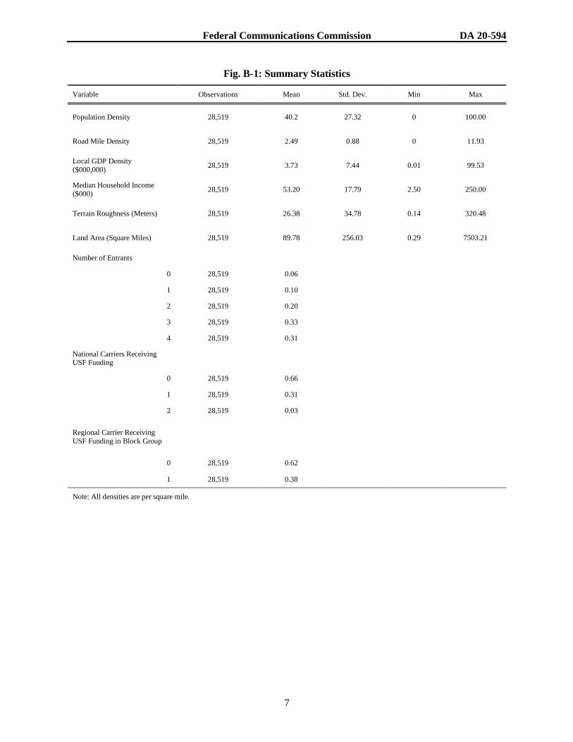
14. Results. Fig. B-2 presents estimation results from twelve specifications of the model.

Columns 1-10 present ordered logit estimates in which the dependent variable is the number of entrants in

the census block group. Our baseline specification is displayed in column 1. Column 2 aggregates

regional carriers’ coverage areas and considers them as a fifth potential entrant. Columns 3 and 4 add

interactions between the demand density variables. Column 5 assumes that the terrain roughness effect

has a logarithmic form. Columns 6 and 7 alter the population density population restriction whereby

column 6 includes block groups with up to 500 persons per square mile and column 7 limits the sample to

block groups with less than 20 persons per square mile. Column 8 uses the population density restriction

in column 7 in lieu of land area weights. Columns 9 and 10 alter the coverage threshold by which census

block groups are determined to be served, using 50% and 90% respectively. Columns 11 and 12 are

simple logit specifications where the dependent variable is a dummy indicating the Census block group

has one or more entrants. Column 11 is the logit analog of the baseline model, while column 12 considers

the regional carriers as potential entrants. In addition to coefficients for the independent variables, Fig. B-

20 We note that while the universal service dummy variables are theoretically included in 𝐶𝑖, we set the dummies to

zero for the representative block groups and thus do not affect 𝐶𝑖.

(continued….)


6

2 also lists the estimated threshold values, which are the levels of latent attractiveness necessary to induce

deployment by an additional provider.21

15. The estimated coefficients on the population, road mile, and local GDP density variables

are positive and statistically significant in all specifications, indicating that Census block groups become

more attractive to entrants when demand density increases and that our model is capturing factors relevant

to carriers’ entry decisions. Similarly, log income is positive and significant in all specifications,

indicating that, all else equal, wealthy areas are more likely to be covered. The negative and significant

dense clutter coefficient indicates that entry is less likely in high clutter areas with greater signal

propagation losses. The estimates also suggest that the multiple carriers receiving universal service

funding dummy variable is capturing otherwise unobserved characteristics that make an area “difficult to

serve.” Areas where multiple national carriers have received funding are likely to have fewer national

carriers enter, however this effect disappears when we consider service as a binary outcome. The

coefficient on the indicator for a regional carrier receiving funding in the area is also negative and

significant. When regional carriers are included in the analysis, the coefficient decreases in magnitude,

suggesting that the areas are unlikely to induce entry by multiple carriers.

16. Fig. B-3 shows the linear spline estimates of terrain roughness on block group

attractiveness for the baseline specification. We find a negative relationship between terrain roughness

and block group attractiveness with the marginal effects decreasing as terrain roughness increases. The

shape of the non-linear relationship is robust across specifications.

17. Fig. B-4 presents the adjustment factor estimates for each category and the corresponding

95% confidence intervals produced by our baseline specification.22 We generate the adjustment factors

using terrain values of 10m, 70m, and 150m, and median household income values of $25,000, $35,000,

and $65,000.23 The baseline specification produces factors ranging from 1 to 4.06. Fig. B-5 presents the

adjustment factors associated with each specification. Across all specifications, the largest factor is

attributed to the mountainous-low median household income category. Top adjustment factors range

from 3.08 to 4.29 with a median value of 3.84. The estimated adjustment factors are generally stable

across specifications. The largest changes occur when we include interaction terms between demand

density variables and when the sample is restricted to block groups with less than 20 persons per square

mile.

21 Note that the estimates in Fig. B-2 do not include a constant term; this is because the first cut point serves as a

constant term in the model. An equivalent approach would be to report a constant term in the regression results and

normalize the first cut point to zero. See Greene (2003) at 787-88.

22 We bootstrap the standard errors to generate the 95% confidence intervals. See Greene (2003) at 652-55.

23 10m, 70m, and 150m are the land area weighted standard deviation of elevation medians of the terrain bins.

Likewise, $25,000, $35,000, and $65,000 are the approximate median values of the income bins.


7

Fig. B-1: Summary Statistics

Variable Observations Mean Std. Dev. Min Max

Population Density 28,519 40.2 27.32 0 100.00

Road Mile Density 28,519 2.49 0.88 0 11.93

Local GDP Density

($000,000) 28,519 3.73 7.44 0.01 99.53

Median Household Income ($000)

28,519 53.20 17.79 2.50 250.00

Terrain Roughness (Meters) 28,519 26.38 34.78 0.14 320.48

Land Area (Square Miles) 28,519 89.78 256.03 0.29 7503.21

Number of Entrants

0 28,519 0.06

1 28,519 0.10

2 28,519 0.20

3 28,519 0.33

4 28,519 0.31

National Carriers Receiving USF Funding

0 28,519 0.66

1 28,519 0.31

2 28,519 0.03

Regional Carrier Receiving

USF Funding in Block Group

0 28,519 0.62

1 28,519 0.38

Note: All densities are per square mile.


8

Fig. B-2: Estimation Results

Dependent Variable = Number of Entrants

Variables (1) (2) (3) (4) (5) (6) (7) (8) (9) (10) (11) (12)

Population Density 0.05*** 0.04*** 0.11*** 0.11*** 0.05*** 0.02*** 0.16*** 0.12*** 0.04*** 0.05*** 0.10*** 0.12***

(0.00) (0.00) (0.00) (0.00) (0.00) (0.00) (0.01) (0.00) (0.00) (0.00) (0.01) (0.01)

Road Mile Density 0.70*** 0.78*** 1.02*** 1.16*** 0.72*** 0.79*** 0.67*** 0.27*** 0.68*** 0.74*** 0.91*** 0.94***

(0.04) (0.04) (0.06) (0.06) (0.04) (0.04) (0.06) (0.04) (0.05) (0.04) (0.11) (0.12)

Local GDP Density 0.04*** 0.03*** 0.05*** 0.06*** 0.04*** 0.06*** 0.03** 0.03** 0.07*** 0.04*** 0.08** 0.07**

(0.01) (0.00) (0.01) (0.01) (0.01) (0.01) (0.01) (0.01) (0.01) (0.00) (0.03) (0.03)

log(Income) 0.51*** 0.60*** 0.49*** 0.59*** 0.52*** 0.58*** 0.32* 0.35*** 0.45*** 0.58*** 0.73*** 0.72**

(0.10) (0.10) (0.10) (0.10) (0.10) (0.09) (0.14) (0.07) (0.11) (0.10) (0.21) (0.22)

% of Land Covered by Dense Clutter -0.02*** -0.02*** -0.02*** -0.02*** -0.02*** -0.01*** -0.02*** -0.02*** -0.01*** -0.02*** -0.03*** -0.03***

(0.00) (0.00) (0.00) (0.00) (0.00) (0.00) (0.00) (0.00) (0.00) (0.00) (0.00) (0.00)

National Carriers Receiving USF

Funding

One 0.23*** 0.29*** 0.14* 0.17** 0.22** 0.23*** 0.18 -0.15** 0.28*** 0.26*** 0.07 -0.08

(0.07) (0.06) (0.07) (0.07) (0.07) (0.06) (0.11) (0.05) (0.07) (0.06) (0.16) (0.18)

Two -0.45*** -0.58*** -0.53*** -0.68*** -0.48*** -0.54*** -0.33* -0.53*** -0.53*** -0.45*** 0.10 -0.04

(0.11) (0.11) (0.11) (0.11) (0.11) (0.11) (0.13) (0.10) (0.11) (0.12) (0.25) (0.27)

Regional Carrier Receiving USF

Funding -0.99*** -0.28*** -1.02*** -0.30*** -0.96*** -0.98*** -0.97*** -1.23*** -1.02*** -0.95*** -0.35* -0.28

(0.07) (0.07) (0.07) (0.07) (0.07) (0.07) (0.10) (0.05) (0.07) (0.06) (0.16) (0.18)

Population Density # Road Mile Density - - -0.00*** -0.00*** - - - - - - - -

- - (0.00) (0.00) - - - - - - - -

Population Density # Local GDP

Density - - -0.02*** -0.02*** - - - - - - - -

- - (0.00) (0.00) - - - - - - - -

Road Mile Density # Local GDP

Density - - 0.01 0.01 - - - - - - - -

- - (0.00) (0.00) - - - - - - - -


9

Dependent Variable = Number of Entrants

Variables (1) (2) (3) (4) (5) (6) (7) (8) (9) (10) (11) (12)

log(Terrain) - - - - -1.15*** - - - - - - -

- - - - (0.03) - - - - - - -

Constant - - - - - - - - - - -0.16 -0.24

- - - - - - - - - - (0.91) (0.98)

Terrain Spline Yes Yes Yes Yes No Yes Yes Yes Yes Yes Yes Yes

Observation Weights Land

Area

Land

Area

Land

Area

Land

Area

Land

Area Land Area

Land

Area None

Land

Area

Land

Area

Land

Area Land Area

Sample <100 Pops

<100 Pops

<100 Pops

<100 Pops

<100 Pops

< 500 Pops

<20 Pops <20 Pops

<100 Pops

<100 Pops

<100 Pops

<100 Pops

Regional Carriers Included No Yes No Yes No No No No No No No Yes

Coverage Threshold 75% 75% 75% 75% 75% 75% 75% 75% 50% 90% 75% 75%

Observations 28,519 28,519 28,519 28,519 28,519 53,041 8,397 8,397 28,519 28,519 28,519 28,519

Threshold 1 -1.33** -0.54 -0.75 0.14 -2.43*** -0.75 -1.99*** -2.79*** -2.20*** -0.53 - -

(0.42) (0.40) (0.43) (0.42) (0.42) (0.38) (0.57) (0.30) (0.44) (0.40) - -

Threshold 2 0.23 0.82* 0.86* 1.56*** -0.88* 0.73 -0.29 -1.14*** -0.36 1.14** - -

(0.42) (0.40) (0.43) (0.42) (0.41) (0.38) (0.56) (0.30) (0.44) (0.40) - -

Threshold 3 1.79*** 2.33*** 2.47*** 3.15*** 0.67 2.19*** 1.37* 0.54 0.99* 2.82*** - -

(0.41) (0.40) (0.43) (0.42) (0.41) (0.38) (0.56) (0.30) (0.44) (0.40) - -

Threshold 4 4.20*** 4.47*** 4.89*** 5.33*** 3.10*** 4.38*** 4.11*** 2.89*** 3.36*** 5.18*** - -

(0.41) (0.40) (0.43) (0.42) (0.41) (0.38) (0.56) (0.30) (0.43) (0.40) - -

Threshold 5 - 7.47*** - 8.26*** - - - - - - - -

- (0.40) - (0.42) - - - - - - - -

Notes: Robust standard errors in parentheses; *** p<0.01, ** p<0.05, * p<0.10 Specs (11) and (12) are logit models where the binary outcome is whether the block group is served by any carrier.


10

Fig. B-3: Terrain Spline Estimates (Specification 1)

Fig. B-4: Adjustment Factor Estimates (Baseline Specification)

Terrain Roughness

Flat Hilly Mountainous

Median Household

Income

Low 1.35 2.81 4.06

[1.25, 1.45] [2.50, 3.12] [3.69, 4.42]

Medium 1.24 2.69 3.96

[1.18, 1.30] [2.40, 2.98] [3.61, 4.30]

High 1 2.40 3.67

[2.14, 2.66] [3.36, 3.98]

95% confidence intervals are shown in brackets.


11

Fig. B-5: Adjustment Factor Estimates (All Specifications)

Terrain Roughness

Flat Hilly Mountainous Flat Hilly Mountainous

(1) (2)

Median

Household

Income

Low 1.35 2.81 4.06 1.35 2.91 4.01 Medium 1.24 2.69 3.96 1.23 2.79 3.90

High 1 2.40 3.67 1 2.52 3.63 (3) (4)

Low 1.25 2.19 3.13 1.27 2.25 3.08 Medium 1.18 2.11 3.06 1.19 2.16 3.01

High 1 1.90 2.86 1 1.95 2.80 (5) (6)

Low 1.34 2.71 3.59 1.43 2.91 4.13 Medium 1.23 2.59 3.49 1.30 2.77 4.01

High 1 2.32 3.23 1 2.39 3.64 (7) (8)

Low 1.16 2.15 3.27 1.30 2.80 4.29 Medium 1.11 2.10 3.23 1.20 2.70 4.21

High 1 1.97 3.10 1 2.45 3.96 (9) (10)

Low 1.38 2.51 3.58 1.36 3.20 4.07 Medium 1.28 2.39 3.49 1.24 3.07 3.96

High 1 2.05 3.16 1 2.76 3.68 (11) (12)

Low 1.36 2.86 3.84 1.32 2.90 3.83 Medium 1.25 2.74 3.75 1.22 2.79 3.74

High 1 2.42 3.44 1 2.50 3.47

II. CELL SITE DENSITY MODEL ADJUSTMENT FACTOR

18. In this section, we estimate the effect of terrain on the number of cell sites required to

build out a mobile wireless network in rural areas. All else being equal, wireless network engineering

principles indicate that greater variability of terrain in a given geographic area reduces the signal strength

received by a mobile user,24 which requires wireless carriers to build more sites to provide the same

quality of service (e.g., speed). Based on county-level cell site counts and coverage data for each of the

four largest national carriers in 2014, we estimate how many more sites must be built per square mile to

cover the same land area in hillier terrain compared to flat areas, holding quality of service fixed.25 If the

24 Campbell Scientific Inc., The Link Budget and Fade Margin, (Sep. 2016), available at

https://s.campbellsci.com/documents/us/technical-papers/link-budget.pdf; William C. Jakes, Microwave Mobile

Communications 126-28 (IEEE Press 1993); Rappaport (2002) at 141-43.

25 Our measure of terrain is the average standard deviation of elevation. See Appx. A: Terrain Elevation for more

details.

(continued….)

https://s.campbellsci.com/documents/us/technical-papers/link-budget.pdf


12

cost of building a site is the same across terrain types, our adjustment factor provides an estimate of how

much more costly it is to deploy mobile broadband in more mountainous areas relative to flatter areas.26

19. To estimate the adjustment factor, we first run a regression that controls for the terrain

variation in the county as well as many other factors expected to affect the service area covered by a site.

Next, from the estimated model, we predict the average number of square miles covered by a typical site

in three terrain categories. Finally, we calculate an adjustment factor by dividing the estimated service

area of a site in a flat area by the estimated service areas in each of the other two terrain categories. Our

results suggest that the hilly terrain category is about 1.5 times more expensive to deploy while the

mountainous terrain category is approximately 2.5-3 times as costly.27

20. Our dependent variable is the average square miles of service area per site in a county for

each national carrier.28 Our key explanatory variable is terrain variability, as measured by the standard

deviation of elevation of the covered land area in a county for each carrier.29 We note that another

important factor to account for is the effect of demand on cell site service areas. In less rural areas with

higher mobile data demand, the size of the cell site service area required to meet the carriers’ minimum

subscriber performance target may be determined by capacity constraints rather than signal propagation

limitations. As a result, in areas of high demand, terrain may have almost no impact on the service area

of a site since the site service area may already need to be quite small due to capacity limits, and therefore

the signal strength would likely be strong throughout the service area of a site regardless of terrain. In

Fig. B-6, we present summary statistics by different subsamples based on population densities for our

dependent and independent variables. Fig. B-7 presents the sample means of our variables by terrain

category and population density subsamples. Since our analysis is mainly concerned with the effect of

terrain in rural areas that are less capacity constrained, we try to minimize the importance of capacity

constraints by restricting the regression estimation to areas with population densities below the same

thresholds that we used in Fig. B-7. Before setting out our regression specification, we briefly discuss the

justification for the inclusion of each of the control variables and how we expect each to affect the

expected squared miles served by a cell site.

A. Network Capacity Constraints

21. Network capacity. The amount of available spectrum bandwidth and the spectral

efficiency of the deployed technology determines the maximum capacity of each site.30 Bandwidth is

determined by the number of megahertz of spectrum that each carrier has deployed per site; greater

bandwidth reduces the number of sites required to serve the same amount of traffic.31 Spectral efficiency

is a function of signal quality and is measured by the bits per second that can be served per hertz of

spectrum.32 More recent technologies, such as 4G LTE and 5G-NR, allow more data to be transmitted

over the same amount of spectrum, and this should allow a carrier to build fewer sites per square mile in

26 If site construction, backhaul, and spectrum acquisition costs do vary by terrain, our estimated factors may not

fully capture the effect of terrain on deployment costs.

27 See infra Fig. B-9.

28 See Appx. B.IV: Data Sources and Variable Construction for more details. Our analysis is restricted to 3,114

counties in the 48 states of the continental U.S., Hawaii, and Washington, D.C. Since our analysis includes the four

largest mobile wireless carriers, we have a potential maximum of 12,456 observations in our sample. We also

anonymize carriers as carrier A, carrier B, carrier C, and carrier D.

29 See Appx. B.IV: Data Sources and Variable Construction for more details. We calculate terrain variation by

carrier since the terrain in the actual land area covered by each carrier in a county may be very different.

30 See T-Mobile-Sprint Order, 34 FCC Rcd at 10764, Appx. F: Technical Appendix, para. 11.

31 OBI Technical Paper No. 1, Exh. 4-Q.

32 OBI Technical Paper No. 1, at.63.

(continued….)


13

capacity constrained areas, all else equal.33 Given a fixed number of sites, the approximate capacity of a

cellular network is therefore given by the following formula.34

𝐶𝑎𝑝𝑎𝑐𝑖𝑡𝑦 = 𝑆𝑖𝑡𝑒𝑠 ∗ 𝐵𝑎𝑛𝑑𝑤𝑖𝑑𝑡ℎ 𝑝𝑒𝑟 𝑆𝑖𝑡𝑒 (𝑀𝐻𝑧) ∗ 𝐸𝑓𝑓𝑖𝑐𝑖𝑒𝑛𝑐𝑦

22. Network Load. Similarly, the network load in a geographic area should also affect the

number of cell sites required.35 If the network traffic served by a site reaches the site’s capacity limit, this

will result in congestion and a degradation in service quality.36 To add capacity in order to maintain the

minimum user speed target, the cell site may then be “split,” which involves covering the same

geographic area with two sites instead of one so that the deployed spectrum can be reused over two

smaller service areas.37 Therefore, for a given capacity per site and quality of service, more sites must be

built closer together in an area with higher traffic demand compared to areas with lower demand.

23. If network capacity is equal to network load, it follows that:

Subscribers ∗ Usage/Subscriber = 𝑆𝑖𝑡𝑒𝑠 ∗ 𝐵𝑎𝑛𝑑𝑤𝑖𝑑𝑡ℎ 𝑝𝑒𝑟 𝑆𝑖𝑡𝑒 (𝑀𝐻𝑧) ∗ 𝐸𝑓𝑓𝑖𝑐𝑖𝑒𝑛𝑐𝑦

Taking the natural logarithm of both sides and rearranging terms yields the following estimation equation

for the number of sites needed in a capacity constrained network environment for a given quality of

service target:

ln(𝑆𝑖𝑡𝑒𝑠) = ln (𝑆𝑢𝑏𝑠𝑐𝑟𝑖𝑏𝑒𝑟𝑠

𝐵𝑎𝑛𝑑𝑤𝑖𝑑𝑡ℎ 𝑝𝑒𝑟 𝑆𝑖𝑡𝑒𝑠) + ln(𝑈𝑠𝑎𝑔𝑒/𝑆𝑢𝑏𝑠𝑐𝑟𝑖𝑏𝑒𝑟) − ln (𝐸𝑓𝑓𝑖𝑐𝑖𝑒𝑛𝑐𝑦)

24. As the number of sites needed to address capacity constraints is a function of the number

of subscribers per megahertz of spectrum, the usage per subscriber and the spectral efficiency of the

deployed technology, we control for each of these factors in our regression model. To account for

subscriber demand and the effect of bandwidth on network capacity, we include the natural logarithm of

the subscribers per megahertz of deployed spectrum in each Cellular Market Area (CMA).38 We would

expect this variable to have a negative sign since, all else equal, more subscribers per MHz should result

in a site being able to cover fewer square miles. We do not have a direct measure of usage per subscriber

in our data sample, so to help alleviate any potential omitted variable bias, we include the natural

logarithm of per capita income as a proxy for subscriber usage.39 To account for spectral efficiency

33 Id.

34 See Applications of T-Mobile USA, Inc., and Sprint Corporation for Consent To Transfer Control of Licenses and

Authorizations, ULS File No. 0008224209 (Lead Application) (filed June 18, 2018, amended July 5, 2018), Exh.

1—Description of the Transaction, Public Interest Statement, and Related Demonstrations at 30. This formula

implies that if the number of sites, bandwidth per site or spectral efficiency doubles, then the overall network

capacity would double as well.

35 Network load is defined here as the product of the number of subscribers served by the site and their usage per

subscriber. For a discussion of how average usage per subscriber maps into busy hour offered load, see OBI

Technical Paper No. 1, at 111.

36 OBI Technical Paper No. 1, at p.109-111.

37 See T-Mobile-Sprint Order, 34 FCC Rcd at 10765, Appx. F: Technical Appendix, para. 14.

38 See Appx. B.IV: Data Sources and Variable Construction for more details.

39 We expect income to be correlated with per subscriber usage, and to be an effective proxy variable, it must also

satisfy the untestable assumption that the regressors are now uncorrelated with the error term once the income

variable is included in the regression. See Jeffrey M. Wooldridge, Introductory Econometrics: A Modern Approach

(Wooldridge (2008)). If income does not sufficiently proxy for usage, the unobserved usage per subscriber variable

could bias our estimated adjustment factors either upwards or downwards, depending on how usage varies with

terrain. If usage is greater in flatter areas than mountainous areas, conditional on our other controls, then our model

would not account for the greater usage shrinking cell coverage in flat areas, and this would tend to bias the

(continued….)


14

differences, we include the percent of the land area in each county that is covered by 4G LTE. We would

generally expect greater spectral efficiency to increase the service area per site in any area that is capacity

constrained but given that deploying more efficient technologies may also increase the unobserved usage

per subscriber, the expected sign of this control variable is ex ante unclear. In order to measure which

counties within a CMA are more likely to have higher network loading, we also include the natural

logarithm of county population density and road mile density. We would expect both variables to have a

negative sign since greater network loading should reduce the square miles covered by a site in capacity

limited areas. Finally, we include the average download speed in each county by carrier, as measured by

2014 Ookla speed test data, to hold service quality fixed.

B. Network Coverage Constraints

25. Propagation model. We use a simple wireless engineering propagation model to inform

our choice of included variables and functional form for our regression analysis. A general form of the

Friis propagation formula for outdoor environments with pathloss due to terrain can be written as

follows:40

𝑃𝑟 = 𝑃𝑡 ∗ 𝑘 ∗ (𝜆

4𝜋)

2

∗1

𝑑𝛼; 𝑜𝑟 𝑑𝛼/2 = (

𝑃𝑡

𝑃𝑟∗ 𝑘)

1/2

∗λ

4𝜋

26. The received power, Pr, is a function of the transmitted power Pt, a constant of

proportionality k that accounts for antennae gains, the transmission wavelength λ and inversely

proportional to the distance from the transmitter d raised to the power α. The parameter α is called the

pathloss exponent and is the focus of our analysis. It measures how quickly the received power declines

as distance from the receiver to the transmitter increases and has a value of two in a free space

environment without obstructions and higher values in more lossy environments. To express this formula

in the logarithmic dB scale, we take the base-10 logarithm of both sides of the equation and then solve for

the logarithm of the maximum distance (cell radius) given a minimum received power threshold.41

𝑙𝑜𝑔10(𝑑𝑚𝑎𝑥) =2𝑙𝑜𝑔10( (

𝑃𝑡𝑃𝑟_𝑚𝑖𝑛

∗ 𝑘)1/2

∗λ

4𝜋)

𝛼

27. The IEEE Stanford University Interim propagation loss model and its extensions

expresses α as a linear function of antenna height and terrain category, where terrain reflects not only the

variation in elevation, but also other factors that affect propagation such as buildings and foliage.42

Therefore, in the Friis propagation model, the service area of a site in a coverage constrained outdoor

environment is a function of, but not limited to, the wavelength (speed of light/frequency) of the deployed

spectrum, tower height, terrain variation and other obstacles that reduce signal propagation such as trees,

foliage, and building structures. Based on this formula we also multiply the logarithm of spectrum

estimated adjustment factor upwards. The terrain adjustment factor would be biased downwards if hillier terrain had

higher usage than flatter areas.

40 See Tony J. Rouphael, RF and Digital Signal Processing for Software-Defined Radio at Section 4.2.1 (2009). For

free space where lambda=2, see Christopher Haslett, Essentials of Radio Wave Propagation at 5-7 (2009). See also

Jyrki T.J. Penttinen, The Telecommunications Handbook, Engineering Guidelines for Fixed, Mobile and Satellite

Systems at 596 (2015).

41 The dB scale is expressed in base-10 logarithms, but we use natural logarithms in our regression analysis. To

convert our estimated regression equations to base-10 logarithms, we would just multiply both sides by

ln(10)=2.303 and this would have no effect on our estimated adjustment factors.

42 V. Erceg et al., An empirically based path loss model for wireless channels in suburban environments 17 IEEE J.

Select. Areas Comm. 1205 (1999).

(continued….)


15

frequency with the terrain variables in our regression analysis since the maximum radius is a

multiplicative function of log10 (λ) and α.

28. Terrain and Clutter. The measure of terrain variability we use in our model is the

standard deviation of elevation of the covered land area in a county for each carrier. In addition to terrain,

radio propagation is affected by the number of man-made and natural obstructions in an area, since these

block, absorb, diffract, and/or reflect radio waves which lead to losses.43 In urban and suburban areas,

signal loss may mostly be due to a greater number of structures that impede radio signals, while in more

rural areas, natural structures such as trees and foliage may be more likely to reduce signal propagation.

We control for “natural” clutter by including the percentage of land area in the county covered with

forests. Clutter from other sources is accounted for by including the natural logarithms of county

population density and business establishment density. We would expect that more densely built-up or

forested areas would require a greater number of sites, and therefore, we expect the sign on these

variables to be negative.44

29. Spectrum Frequency and Tower Height. Lower frequency spectrum can travel farther

and better penetrate natural and other obstacles, which allows a carrier to cover a larger area with fewer

sites absent capacity constraints.45 We control for the frequency of spectrum deployed by including an

indicator variable if the carrier has deployed low-band spectrum in the county and interact it with our

measure of terrain variation and the percentage of forested area in the county to allow the effect of these

variables on site coverage to vary by the frequency of deployed spectrum.

30. Tower height was not available in our cell site dataset, so to estimate the height of each

tower in our sample, we compiled tower height information from publicly available tower company

sources.46 We first drop all towers with missing height information or a listed height over 500 feet in the

tower company dataset since these are outliers that likely have inaccurate height information. We then

match the towers in our sample to the closest tower in the public dataset and assign the tower height of the

closest matched tower as long as that tower lies within 1 kilometer of the tower from the original data

sample.47 For towers that do not match within 1 kilometer, we assign the average tower height of the

matched towers in the county for that carrier.

31. Other Control Variables. We also include carrier fixed effects in the model to capture

any differences across carriers that do not vary at a sub-national level and eliminate potential bias from

these unobserved differences across carriers. For example, if some carriers have higher data usage limits

on their plans, and these plan characteristics are set nationally, then these carriers may have higher data

usage per subscriber and would generally need more cell sites to serve their subscribers than a carrier with

lower data limits, all else equal. Other important company-level policy differences across carriers such as

43 See OBI Technical Working Paper No. 1, at 68.

44 In addition to propagation, these variables may also be controlling for differences in demand that are not fully

accounted for by our inclusion of CMA subscribers and the other demand measures noted above. These effects

reinforce the propagation effects since we would also expect areas with greater demand to require more sites.

45 See OBI Technical Working Paper No. 1, at 67.

46 Tower site information was downloaded from 44 tower providers’ websites in May 2018. Wireless Estimator,

Top 100 Tower Companies in the U.S., http://www.wirelessestimator.com/t_content.cfm?pagename=US-Cell-

Tower-Companies-Complete-List (last visited May 15, 2020). Publicly available tower data with height information

for the same time period as the BDS data was not available. However, we do not expect this to have much effect on

our analysis since we are matching towers to themselves, and it is unlikely that many towers have been

decommissioned in the intervening four years.

47 A 1-kilometer buffer is used since differences in geocoding between the two data sources may result in a tower

not matching exactly to itself. With this buffer, our match rate for towers within 1 km was approximately 82%.

(continued….)

http://www.wirelessestimator.com/t_content.cfm?pagename=US-Cell-Tower-Companies-Complete-List



16

the criteria they use to determine when a cell site needs to be split would also be captured in these carrier

fixed effects.

32. In some of our specifications, we also add state fixed effects to the model so that only the

variation in terrain within a state is being used to estimate the relationship between average square miles

covered per site and terrain. Including state fixed effects will eliminate potential bias due to unobserved

differences across states that impact site service areas and are correlated with our control variables. For

example, if some states have more restrictive regulations on site deployment, then this could

systematically lower the number of sites built in all counties located within that state. The inclusion of

state fixed effects would ensure that such differences between states do not bias our adjustment factor

estimates.

C. Regression Results

33. Each observation in our dataset is a county-carrier combination (e.g., Autauga County,

carrier A), and our dependent variable is the natural logarithm of the average square miles served per site

in the county for each carrier.48 We take two approaches to account for the effect of subscriber demand

and capacity constraints on the average per site service area. The first is to estimate a model with a

flexible functional form that allows the effect of terrain to decline as capacity constraints increase by

interacting the terrain variable with subscribers per megahertz of spectrum. We expect this interaction

term to have a positive coefficient since per site service areas in counties with less spectrum per

subscriber are more likely to be constrained for capacity reasons rather than coverage reasons related to

propagation. The second approach, which we prefer, is to restrict our estimation sample to more rural

counties. This is done by estimating the model on sub-samples of counties with population densities less

than 100, 50 and 20 people. In the specifications run on the restricted samples, we expect the interaction

between terrain and subscribers per MHz to be less important since in these areas of lower subscriber

demand the service areas of these sites will more likely be propagation constrained rather than capacity

constrained. The estimated model for the natural logarithm of the expected average service area per site

in county i carrier j, in CMA k, and state m is as follows:

ln(𝐶𝑜𝑣𝑒𝑟𝑎𝑔𝑒𝐴𝑟𝑒𝑎𝑃𝑒𝑟𝑆𝑖𝑡𝑒𝑖𝑗𝑘𝑚)

= 𝛽0 + 𝛽1𝑇𝑒𝑟𝑟𝑎𝑖𝑛𝑖𝑗 + 𝛽2𝑃𝑜𝑝𝐷𝑒𝑛𝑖 + 𝛽3 ln(𝑅𝑀𝐷𝑒𝑛𝑖) + 𝛽4 ln(𝐸𝑠𝑡𝐷𝑒𝑛𝑖)

+ 𝛽5 ln(𝐼𝑛𝑐𝑜𝑚𝑒𝑖) + 𝛽6 ln(𝑆𝑢𝑏𝑠𝑃𝑒𝑟𝑀𝐻𝑧𝑗𝑘) + 𝛽7 ln(𝑆𝑢𝑏𝑠𝑃𝑒𝑟𝑀𝐻𝑧𝑗𝑘) 𝑋 𝑇𝑒𝑟𝑟𝑎𝑖𝑛𝑖𝑗

+ 𝛽8𝑃𝑒𝑟𝑐𝐴𝑟𝑒𝑎𝐿𝑇𝐸𝑖𝑗 + 𝛽9𝑃𝑒𝑟𝑐𝐴𝑟𝑒𝑎𝐹𝑜𝑟𝑒𝑠𝑡𝑖 + 𝛽10𝐿𝑜𝑤𝐵𝑎𝑛𝑑𝑖𝑗

+ 𝛽11𝐿𝑜𝑤𝐵𝑎𝑛𝑑𝑖𝑗𝑋 𝑃𝑒𝑟𝑐𝐴𝑟𝑒𝑎𝐹𝑜𝑟𝑒𝑠𝑡𝑖 + 𝛽12𝐿𝑜𝑤𝐵𝑎𝑛𝑑𝑖𝑗𝑋 𝑇𝑒𝑟𝑟𝑎𝑖𝑛𝑖𝑗

+ 𝛽13 ln(𝐷𝑜𝑤𝑛𝑆𝑝𝑒𝑒𝑑𝑖𝑗) + 𝛽14𝑇𝑜𝑤𝑒𝑟𝐻𝑒𝑖𝑔ℎ𝑡𝑖𝑗 + 𝛽15𝑃𝑟𝑜𝑣𝑗 + 𝛽16𝑆𝑡𝑎𝑡𝑒𝑚 + 𝜀𝑖𝑗

34. Fig. B-8 shows the regression results from models with and without state fixed effects on

the full and population density restricted samples. The coefficients on nearly all variables are generally

consistent with our expectations based on the Friis propagation formula we derived. The coefficients on

both the terrain and the percentage of the county that is forested variables are negative and statistically

significant, implying that the average service area of a site decreases as terrain becomes more

mountainous and forested. Similarly, as the number of subscribers per megahertz of spectrum, density of

establishments, road miles, or population increases, the expected average area served by a site decreases.

Deploying low band spectrum both increases the expected average service area of a site and reduces the

impact of terrain and clutter as shown by the positive sign on the interaction of low band spectrum and

these variables. Finally, the percentage of area covered by 4G LTE and the income variables are

generally insignificant and of indeterminant sign.

48 We chose the county as our geographic unit of analysis because we do not observe the actual geographic service

area of each site. The choice of county minimizes the number of sites with coverage that crosses the geographic

boundary while still maintaining necessary terrain variation.


17

D. Adjustment Factor Estimates

35. We now predict the average service area of a site at various levels of terrain variation,

setting population density, road mile density, establishment density, and subscribers per megahertz of

deployed spectrum at the 5th percentile of the estimation sample restricted to less than 100 people per

square mile. We chose to predict at the 5th percentiles to remove all potential capacity constraint issues

from our estimated site service areas for each terrain category.49

36. The dependent variable in our regression is the natural logarithm of service area per site.

However, in calculating the adjustment factor, we are interested in the level of service area per site, not

the logarithm of the service area. In general, exponentiating the predicted service areas from the log

model will not recover the correct predictions for service areas by terrain category.50 As a result, when

we exponentiate to form predicted service areas per site, we have to account for the expectation of exp[ε],

or our predicted values for coverage will be biased downward. We assume that the error term has a log-

normal distribution, which gives the following equation for our predicted coverage values:51

�� = exp(𝑙𝑜𝑔��) ∗ exp (0.5 ∗ 𝜎2)

where 𝑙𝑜𝑔�� is the predicted logarithm of average county service area for each carrier and σ2 is the root

mean squared error (RMSE) of the model.

37. Fig. B-9 shows the predicted service areas from each specification, the implied radii, and

adjustment factors and their 95% confidence intervals.52 Our eight specifications produce consistent

adjustment factors ranging from 2.13 to 2.96 for the mountainous terrain category, and our preferred

specifications that restrict population density all produce mountainous adjustment factors of 2.49 or

greater. For example, for our specification that includes state fixed effects and limits the sample to less

than 20 people per square mile (bottom right panel), the high adjustment factor implies that a site in flat

terrain (10m) can cover 2.96 times more area on average than the average land area covered by a site in a

mountainous area (150m).

38. Using county level coverage and site data from each of the four largest carriers, we

calculated adjustment factors based on a model that estimates how the average service area of a site

changes according to the terrain of the surrounding area. If deployment costs are not affected by terrain,

then our estimated adjustment factors will measure the cost differences of deploying a wireless network

across terrain types. However, deployment costs most likely differ across terrain types, and therefore, our

adjustment factors may not fully capture the cost differences. The direction of this bias is unclear. On the

one hand, backhaul, power, and siting costs may be more expensive in hillier terrain compared to flatter

areas. On the other hand, spectrum acquisition costs may be lower in mountainous areas compared to

flatter, more populated areas. While the former considerations would imply that we are understating our

adjustment factors, the latter would imply they are overstated. Despite this issue, we believe that our

results can help inform the Commission regarding the magnitude of cost differences of deploying mobile

49 The estimated adjustment factors are all measured relative to coverage per site in a flat area. For this reason, the

values of the control variables at which we choose to predict the model generally do not affect the estimated

adjustment factors. However, the low band indicator variable and subscribers per megahertz are interacted with

terrain in the model so that the values chosen for these variables in predicting site service areas in each of the terrain

categories do affect the estimated adjustment factors.

50 See Arthur S. Goldberger, The Interpretation and Estimation of Cobb-Douglas Functions. 36 Econometrica 464

(1968).

51 See Wooldridge (2008) at 210.

52 We use a bootstrap procedure to calculate the confidence intervals for the adjustment factors. This procedure

drew 1000 bootstrap replicates with replacement from the data and then re-estimated the regression model to

estimate the sampling distribution from which we calculate the confidence intervals of the unknown parameters.


18

broadband services in different terrain types and provide the Commission with further evidence on what

adjustment factors may be appropriate for the upcoming 5G Fund auction.

Fig. B-6: Summary Statistics by Population Density Subsample

Mean Minimum Maximum

None < 100 < 50 < 20 None < 100 < 50 < 20 None < 100 < 50 < 20

Coverage Area per Tower

(Sq. Miles)

113 164 211 338 0.0 0.5 0.5 0.5 3,047 3,047 3,047 3,047

Terrain (Meters) 22 24 25 31 0.2 0.3 0.3 0.3 213 213 213 212

Population Density

(Population per Sq. Mile) 348 39 23 9.2 0.2 0.2 0.2 0.2 71,481 100 50 20

Road Mile Density

(Road Miles per Sq. Mile)

3.4 2.3 2.1 1.8 0.4 0.4 0.4 0.4 26 5.7 5.2 3.4

Establishment Density

(Establishments Per Sq. Mile) 9.8 0.8 0.5 0.2 0.004 0.004 0.004 0.004 4,643 5.6 3.6 1.6

Median Household Income

(Thousands of 2013 Dollars)

47 43 42 43 21 21 21 21 122 83 83 82

Subscribers per MHz Deployed

Spectrum (CMA)

1,752 531 449 383 0.3 0.3 1.1 1.1 69,943 30,406 14,000 7,362

Pct. Area Covered by 4G-LTE 48% 40% 37% 34% 0% 0% 0% 0% 100% 100% 100% 100%

Pct. Area Covered by Forest 37% 37% 34% 24% 0.0% 0.0% 0.0% 0.0% 93% 93% 93% 93%

Pct. Counties with Low Band

Spectrum Deployed 81% 83% 85% 87% 0% 0% 0% 0% 100% 100% 100% 100%

Avg. Download Speed (Mbps) 12 11 11 11 0.01 0.01 0.01 0.01 110 48 48 44

Avg. Tower Height (Meters) 66 73 75 74 4 4 4 4 152 152 152 152

Number of Observations 9,190 5,836 3,929 1,720

Fig. B-7: Sample Means by Terrain Categories and Population Density Subsamples

Flat Terrain (0-40m) Hilly Terrain (40-115m) Mountainous Terrain (115+m)

Population Density Restriction

None < 100 < 50 < 20 None < 100 < 50 < 20 None < 100 < 50 < 20

Service Area per Site

(Sq. Miles)

109 161 206 337 132 180 250 380 148 156 167 209

Terrain Roughness

(Std. deviation of elevation)

12 11 11 12 68 70 71 73 142 143 145 144

Population Density

(Population per Sq. Mile) 387 40 24 10 157 38 20 7.3 39 23 17 8.8

Road Mile Density

(Road Miles per Sq. Mile)

3.5 2.4 2.2 1.9 2.8 2.2 1.9 1.5 1.9 1.7 1.6 1.4

Establishment Density

(Establishments per Sq. Mile) 11.1 0.8 0.5 0.2 3.9 0.9 0.4 0.2 1.2 0.8 0.7 0.4

Median Household Income

(Thousands of 2013 Dollars)

46.7 42.4 41.5 42.4 48.0 44.6 44.7 45.2 50.1 49.8 50.9 49.0

Subscribers per MHz Deployed

Spectrum (CMA)

1,766 518 422 351 1,776 558 523 472 865 766 756 517

Pct. Area Covered by 4G-LTE 52% 44% 42% 40% 30% 22% 19% 16% 17% 15% 14% 10%

Pct. Area Covered by Forest 34% 34% 31% 19% 49% 49% 42% 31% 60% 60% 59% 56%

Pct. Counties with Low Band

Spectrum Deployed 82% 84% 85% 88% 78% 79% 80% 82% 85% 85% 85% 88%

Avg. Download Speed (Mbps) 12 12 12 12 10 10 10 9.0 8.8 8.7 8.4 7.9

Avg. Tower Height (Meters) 70 79 82 85 47 49 47 43 32 31 30 30

Number of Observations 7,702 4,767 3,198 1,294 1,325 915 593 331 163 154 138 95


19

Fig. B-8: Regression Estimates of the Natural Logarithm of Average Coverage Area

on Capacity and Coverage Factors

Model 1 Model 2 Model 3 Model 4 Model 5 Model 6 Model 7 Model 8

State Fixed Effects No No No No Yes Yes Yes Yes

Population Density Restriction None 100 50 20 None 100 50 20

Carrier-Specific Terrain -0.010 -0.011 -0.010 -0.008 -0.010 -0.011 -0.009 -0.009

(.002) (.002) (.002) (.003) (.002) (.002) (.002) (.002)

*** *** *** *** *** *** *** ***

Log(Population Density) -0.339 -0.398 -0.411 -0.336 -0.259 -0.304 -0.309 -0.257

(.032) (.034) (.038) (.054) (.032) (.034) (.039) (.054)

*** *** *** *** *** *** *** ***

Log(Road Mile Density) -0.389 -0.155 -0.169 -0.093 -0.335 -0.020 -0.043 0.040

(.047) (.059) (.059) (.063) (.035) (.041) (.044) (.060)

*** ** *** ***

Log(Establishment Density) -0.201 -0.087 -0.029 -0.028 -0.279 -0.183 -0.129 -0.107

(.030) (.033) (.037) (.048) (.029) (.033) (.035) (.046)

*** *** *** *** *** **

Log(Income) 0.013 -0.080 -0.055 0.030 0.036 -0.151 -0.157 -0.061

(.045) (.061) (.072) (.095) (.040) (.053) (.069) (.093)

*** **

Log(Subscribers per Deployed MHz)

(CMA Level)

-0.100 -0.083 -0.067 -0.070 -0.101 -0.079 -0.066 -0.072

(.012) (.013) (.017) (.025) (.010) (.012) (.016) (.023)

*** *** *** *** *** *** *** *** Terrain*Log(Subscribers per Deployed

MHz) (CMA Level) 0.001 0.002 0.001 0.001 0.001 0.002 0.001 0.001

(.000) (.000) (.000) (.000) (.000) (.000) (.000) (.000)

*** *** *** ** *** *** *** **

Percentage of Area Covered by 4G-LTE 0.035 0.051 -0.026 -0.162 0.015 0.049 -0.027 -0.113

(.051) (.058) (.062) (.116) (.047) (.057) (.063) (.117)

Percentage of Area Forested -0.979 -1.309 -1.387 -1.489 -0.862 -1.139 -1.176 -1.086

(.166) (.126) (.124) (.284) (.143) (.120) (.127) (.307)

*** *** *** *** *** *** *** ***

Low Band Spectrum Deployed Flag -0.029 0.105 0.101 0.073 -0.054 0.063 0.050 0.069

(.079) (.084) (.090) (.127) (.075) (.095) (.099) (.137)

Low Band Spectrum Deployed

Flag*Percentage of Area Forested

0.155 0.300 0.403 0.541 0.190 0.328 0.415 0.439

(.178) (.148) (.151) (.288) (.147) (.132) (.141) (.287)

** *** * ** ***

Low Band Spectrum Deployed

Flag*Terrain

0.002 0.001 0.001 0.000 0.001 0.001 0.001 0.000

(.002) (.001) (.001) (.002) (.001) (.001) (.001) (.002)

Log(Download Speed) -0.061 -0.048 -0.060 -0.093 -0.055 -0.038 -0.045 -0.061

(.014) (.013) (.015) (.023) (.012) (.012) (.014) (.023)

*** *** *** *** *** *** *** ***

Average Tower Height 0.004 0.002 0.002 0.000 0.003 0.003 0.002 0.001

(.001) (.001) (.001) (.001) (.001) (.001) (.001) (.001)

*** *** ** *** *** ***

Sample Size 9,190 5,836 3,929 1,720 9,190 5,836 3,929 1,720

R-Squared 0.85 0.64 0.59 0.47 0.86 0.66 0.62 0.52

Robust standard errors in parentheses are clustered at the state-provider level.

***p<0.01, **p<0.05, *<0.1


20

Fig. B-9: Regression Model Predictions of Average Coverage Areas, Average Radius,

and Terrain Factors

Terrain Value Cov. Area (Sq. Mile) Radius (Miles) Terrain Factor 95% CI LB 95% CI UB Cov. Area (Sq. Mile) Radius (Miles) Terrain Factor 95% CI LB 95% CI UB

10 123 7 1.00 … … 117 7 1.00 … …

70 84 6 1.47 1.34 1.59 83 6 1.42 1.30 1.54

150 54 5 2.27 1.80 2.73 55 5 2.13 1.70 2.56

10 129 7 1.00 … … 128 7 1.00 … …

70 82 6 1.58 1.43 1.73 82 6 1.55 1.40 1.70

150 49 4 2.65 2.05 3.26 49 4 2.59 2.00 3.18

10 130 7 1.00 … … 132 7 1.00 … …

70 84 6 1.55 1.38 1.72 86 6 1.54 1.36 1.71

150 51 4 2.55 1.89 3.20 52 4 2.54 1.86 3.21

10 150 8 1.00 … … 177 8 1.00 … …

70 98 6 1.53 1.32 1.75 108 6 1.63 1.40 1.86

150 60 5 2.49 1.67 3.31 60 5 2.96 1.95 3.97

95% confidence intervals calculations computed using bootstrap procedure and are based on 1000 replicates.

Site radius calculations assume a hexagonal coverage areas equal to 2.598 the square of the radius.

< 100 Pops / Sq. Mile < 100 Pops / Sq. Mile


No Population Density Restriction No Population Density Restriction

Without State Fixed Effects


With State Fixed Effects

Evaluation Parameters: Population density, road mile density, establishment density, download speed, income, and tower height are evaluated at the mean of the < 100 pops sample; subscribers per deployed

MHz is evaluated at the 5th percentile of the <100 pops sample; percentage forested is evaluated at the mean of each terrain category in the <100 pops sample; Low Band Spectrum Deployed Flag set to 1;

Percentage of Area Covered by LTE set to 100%; Provided and state fixed effects are evaluated at means of regression samples.

III. AUCTION BIDDING MODEL ADJUSTMENT FACTOR

39. This section uses Mobility Fund Phase I auction data to estimate the effects of terrain and

other factors on the requested subsidy amounts for carriers to deploy mobile wireless infrastructure in

previously unserved areas. The Mobility Fund Phase I auction was a reverse auction in which firms bid

for subsidies to provide mobile service to all road miles in an unserved geographic area.53 A higher bid

means a higher subsidy is required for a firm to want to serve the area, which either means the cost to

serve the area is high, the expected revenue is low, or the bidder expects less competition from other

bidders. In this section, we regress the observed bids on area-specific variables that account for

differences in expected costs and revenues to serve the area and competition in the auction. We find that

terrain has a substantial and statistically significant effect on the requested subsidy amount requested by

carriers.54

40. Background. In the Mobility Fund I proceeding, the Commission established Auctions

901 and 902 to distribute universal service funds to areas that lacked sufficient mobile service.55 The

analysis uses September 2012 bidding data from Auction 901. Bidders in the auction submitted sealed

bids indicating the subsidy they would accept to serve all unserved road miles in a given geographic

53 Mobility Fund Phase I Auction Scheduled for September 27, 2012, Notice and Filing Requirements and Other

Procedures For Auction 901, Public Notice, 27 FCC Rcd 4725, 4729, para. 8 (2012) (Auction 901 Procedures

Public Notice).

54 We estimate the elasticity of bids amount to our measure of terrain roughness to be between 0.16-0.23. The small

sample limits our ability to draw strong conclusions about the impact of other factors on bid amount.

55 Auction 901 occurred for most areas on September 27, 2012 with a budget of $300 million, and Auction 902

occurred specifically for Tribal areas on February 25, 2014 with a budget of $50 million. See Connect America

Fund et al., Report and Order and Further Notice of Proposed Rulemaking, 26 FCC Rcd 17663, 17675, para. 28

(2011) (USF/ICC Transformation Order); Auction 901 Procedures Public Notice, 27 FCC Rcd at 4727, para. 1;

Tribal Mobility Fund Phase I Auction Rescheduled for February 25, 2014 Notice of Changes to Auction 902

Schedule Following Resumption of Normal Commission Operations, Public Notice, 28 FCC Rcd 14656, 14656,

para. 1 (2013). We do not consider Auction 902 because Tribal entities received bidding credits for Tribal areas,

which would complicate the analysis, and we exclude Tribal areas in Auction 901 for the same reason.

(continued….)


21

area.56 In our estimation sample, the geographic areas were all Census tract aggregations of unserved

road miles.57 The auction was conducted in a single round with bids simultaneously accepted for all areas

and winning bids were determined by an algorithm that favored lower bids on a per road mile basis, but

also kept total awarded bids within a budget.58

41. Regression Specification. Bids in an auction for subsidies should reflect the relative

profitability of the geographic areas for auction. Those geographic areas that bring in more revenue and

cost less to serve should require a lower subsidy to induce the bidder to serve, and, accordingly, such

areas should receive lower bids, all else equal. We use linear regression to estimate the following

specification of the effect of various revenue and cost factors on bids:

ln(𝐵𝑖𝑑𝑖𝑗) = 𝑋𝑖𝑗𝛽 + 𝜙𝑗 + 𝜖𝑖𝑗

42. We assume the natural logarithm of the dollar per road mile bid (log bids) is a function of

expected revenue and cost factors, 𝑋𝑖𝑗, plus bidder level fixed effects, 𝜙𝑗, where i indicates a specific

geographic area and j indicates the bidder. These factors include our measure of terrain roughness, area

demographics and variables designed to capture competitive aspects of bidding and competition in the

service market. The vector 𝛽 represents the collective effects of the individual factors. We use log bids

because the distribution of bids is highly skewed, and the log transformation makes the resulting data fit a

normal distribution more closely, and thus better meets the classical assumptions for linear regression. In

addition, because many skewed factors in 𝑋𝑖𝑗 are also log-transformed, most of the coefficients in 𝛽 can

be interpreted as elasticities; i.e. a coefficient 𝛽𝑘 of a factor 𝑋𝑖𝑗𝑘 implies a 𝛽𝑘 percent change of the dollars

per road mile bid with a 1 percent change in that untransformed factor. The bidder-level fixed effects, 𝜙𝑗,

represent differences in costs and productivity that are entirely specific to the bidders themselves, and are

not reducible to the observable characteristics of the geographic area or bidders. Finally, 𝜖𝑖𝑗 represents

the impact of any other determinants of bid level, such as cost or revenue factors specific to the area, that

are not observed in any dataset to which we have access.

43. Sample. Our estimating equation is more likely to be appropriate when areas included in

the data set are generally more comparable, so we exclude a variety of areas from the sample to maximize

the comparability of geographic areas and bids.59 The 5,695 potential areas generated 517 bids, with only

24 areas attracting more than 1 bid. Fifty-two areas with bids were not assigned any subsidy because the

bids were so high the assignment algorithm could not grant them without exceeding the budget.

56 Auction 901 Procedures Public Notice, 27 FCC Rcd at 4761-65, paras. 131-141.

57 Eligible areas were U.S. Census blocks that lacked 3G or better mobile coverage at the centroid of the block and

contained road miles in any of six road categories. These blocks were identified by analyzing American Roamer

coverage data (now called Mosaik). USF/ICC Transformation Order, 26 FCC Rcd at 17783-84, paras. 332, 334.

58 The algorithm considered the lowest bids in an area to be tentatively winning bids. The algorithm then ranked

the areas in ascending order by their tentatively winning bids on a per-road mile basis. As it went through the

ranking, the algorithm awarded subsidies (equal to the per-road mile bid times the road mile service requirement) if

that item had not been previously assigned and the total requested subsidies did not exceed the Mobility Fund Phase

I budget. Auction 901 Procedures Public Notice, 27 FCC Rcd at 4765-66, paras. 143-44.

59 Data on all Auction 901 results are available online. Auction 901: Mobility Fund Phase I,

https://www.fcc.gov/auction/901 (last visited May 15, 2020). Specifically, the sample excludes: (1) areas in Alaska

since these are especially large and not tract based; (2) awards to Tribal entities, since they received bidding credits

for Tribal areas; (3) areas in Guam and the Northern Mariana Islands because we do not have terrain data there; (4)

one very small area, T37171930102, for which it is difficult to calculate terrain roughness; and (5) area

T37171930101 in North Carolina because it is made up of 3 disjoint and small parts. Auction 901 Procedures

Public Notice, 27 FCC Rcd at 4763-64, paras. 138-40.

(continued….)

https://www.fcc.gov/auction/901


22

44. Out of 517 bids, 225 led to eventual defaults. It is unclear whether defaulted bids

accurately reflect the true effect of cost and demand factors on bid amounts, as these bids may have

greatly underestimated the required subsidy to make service of the given area viable. Similarly, bids that

failed to receive subsidies may be systematically biased upwards given they may imply a higher estimate

of costs or lower estimates of revenues than the bids that won subsidies. Given the difficulties in

knowing whether to remove “potentially unreasonable” bids systematically, in addition to reporting

results for the full sample, we will also report results for 1) the sample of bids with no defaults and 2) the

sample of bids without defaults or losing bids.

45. Since they likely acted as a single strategic entity, we group subsidiaries into a single

firm. This results in 19 active bidders for our subsample, 8 active bidders who bid outside of our

subsample, and 9 bidders who applied but did not ultimately bid. Finally, we note that this sample of bids

is a selected sample of only the areas that received at least one bid. If our cost and demand factors are

correlated with the unobserved shock, 𝜖𝑖𝑗 then our linear regression estimates will be biased. The

decisions of bidders on where to bid could induce such correlation because observable factor

combinations that would otherwise predict negative bids (low 𝑋𝑖𝑗𝛽) are included only if they have a high

and positive, unobservable shock.60 Therefore, our results should be interpreted with caution.

46. Data. The summary statistics are presented in Fig. B-10. The dependent variable is the

dollar per road mile bid amount, which is how the bids were submitted.61 Bids are right skewed, with

winning bids having a mean of $8,135 per road mile and a median of $5,815 per road mile, while losing

bids have a mean and median bid amount of $74,816 per road mile and a median of $49,312 per road

mile, respectively. There was also substantial variation in bid amount. On a per road mile basis, the

upper limit for winning bids was $41,523, but bids were as high as $429,695 and as low as $130.

47. We use many of the independent variables that were used in the Entry Model as

described above as cost/revenue factors. These include logs of our measure of terrain roughness,

population density, tract median household income, road miles, and percent forested land.62 Terrain

roughness will capture the effect of terrain on increased construction costs and reduced signal propagation

distances. The other demographic and economic variables proxy for wireless demand for and cost

variation caused by differences in economic development. Total road miles is also included to capture

potential economies and diseconomies of scale in network infrastructure construction.

48. Our independent variables also include the fraction of a tract that is forested since forests

would tend to reduce signal propagation and increase construction costs.63 We also include separate

variables for the fraction of the tract for which any service carrier and the bidder already provide some

level of service, as measured by January 2012 coverage data. 64 If the surrounding area is well served by

the bidder, we would expect they would have lower costs of expanding coverage. When the area is

already well covered by other firms, represented by overall coverage, then rival firms are likely to be

strong future competitors in the area to be served which may raise the required subsidy. We also include

the number of carriers in the tract to measure local competition in the downstream market that would

reduce revenues.65 Similarly, we include the potential number of bidders as a covariate. While multiple

60 The direction of the bias on estimated coefficients is only known under special circumstances. See Arthur S.

Goldberger, Linear regression after selection, 15 J. Econometrics 357 (1981).

61 See infra Appx. B.IV: Data Sources and Variable Construction for information on the data sources and

construction of the variables.

62 Id.

63 Id.

64 Id.

65 Id.

(continued….)


23

bids for the same area were rare, the mere threat of a bid by a competitor may be enough to lower the bids

that do occur. To calculate the number of potential bidders, we use bidder applications submitted to the

Commission before the auction.66

49. Some of the independent variables, the average number of carriers, the number of carriers

and the preexisting coverage variables, are calculated on a geographic basis.67 Land area is the most

common basis on which to calculate these variables, but since bidding was done on a road miles basis, the

number of road miles basis may be the most relevant. We produce estimates using both approaches and

find little difference between the results.

50. Results. We estimate six specifications, and our results are presented in Fig. B-11 below.

Specifications (1)-(3) use the land area basis for some variables and (4)-(6) use the road miles basis.

Specifications (1) and (4) include all observations, (2) and (4) exclude defaults, and (3) and (6)

additionally exclude losing bids. Across all specifications, our terrain measure has between a 0.16 to 0.23

elasticity with respect to bids that is statistically significant across all specifications. That is, for every

1% increase in terrain roughness, we have a 0.16% to 0.23% increase in the dollar per road mile bid.

Dividing terrain roughness into three categories of 0-40 m (flat), 40-115 m (hilly) and 115+ m

(mountainous), we estimate the adjustment factor for each bin by estimating the impact of terrain

roughness on the per road mile bids in levels at the same terrain values of 10m, 70m, and 150m used in

the entry and cell site density analyses.68 That is, the adjustment factor is the model predicted per road

mile bid amount at one of these terrain levels over the predicted bid amount at 10 m. Holding all other

variables fixed, this ratio will be constant for our formula across all possible areas and bidders.69 Using

the estimates of the full sample, the three categories would have adjustment factors of approximately 1.0

(0-40 m), 1.6 (40-115 m) and 1.9 (115+ m).

51. Several other covariates have statistically significant results over all or most of the

specifications. Road miles has a negative impact on dollars per road mile, with an implied elasticity

between -0.24 to -0.47. This result is consistent with economies in scale in road miles for wireless

infrastructure, though the effect is not statistically significant in specification (6), the subsample with

variables weighted over road miles and with no defaults or losing bids. Likewise, a bidder’s current tract

network coverage also seems to reduce costs, whereby an additional 1% network coverage is associated

with between a 0.36% and 0.55% decrease in the bid, though the coefficient is not statistically significant

for the sample with no defaults but no losing bids and using area-based variables. The percent coverage

of the tract by forested land has a statistically significant large positive impact on bid amount, but not for

specifications using the full sample. This may imply that defaulting bidders underestimated the

importance of clutter in their bid calculations.

52. Other coefficients are too imprecisely estimated to draw further conclusions, probably

due to the small sample size and limited variation of the sample. Population density has small implied

elasticities between -0.2 and -0.7, which are only significant using the sample without defaults but with

losing bids. The log count of carriers has coefficients that are mostly larger than the ones for terrain,

between 0.20 and 0.38, but are only statistically significant for specifications using the sample without

66 Id.

67 Log count of carriers was calculated as a log of the weighted average count, not the weighted average of logs.

68 These categories are consistent with the earlier categories used in the Entry Model and the Cell Site Density

Model. See supra Appx. B.I: Entry Model Adjustment Factor and App. B II: Cell Site Density Model Adjustment

Factor.

69 If T is the terrain roughness in the comparison category, and 𝛼 is the coefficient on the natural logarithm of terrain

roughness, then the adjustment factor for this category is the expectation of the ratio between what a given bid

would be if we changed the terrain roughness to 𝑇 meters over that bid if we changed the terrain roughness to 10

meters: 𝐸 [𝐵𝑖𝑑𝑖𝑗 𝑎𝑡 𝑇 𝑚

𝐵𝑖𝑑𝑖𝑗 𝑎𝑡 10 𝑚] = 𝐸 [

𝑇𝛼 𝑒𝑥𝑝(𝛽𝑋𝑖𝑗−𝛼 ln( 𝑇𝑖𝑗)+𝜙𝑗+𝜖𝑖𝑗)

10𝛼 𝑒𝑥𝑝(𝛽𝑋𝑖𝑗−𝛼 ln(𝑇𝑖𝑗)+𝜙𝑗+𝜖𝑖𝑗)] = (

𝑇

10)

𝛼

.


24

defaults and losing bids, and for the specification using losing bids but no defaults and using area-based

variables. Coverage by any carrier has relatively large negative coefficients using the full sample but no

coefficient in any specification is statistically significant. Consistent with competition reducing bids, the

coefficients on potential bidders are mostly negative, though only the coefficients on “Two bidders” were

statistically significant and only for the sample removing defaults and losing bidders. Finally, log median

household income always has a positive coefficient, which runs counter to the idea that more economic

activity would make an area more profitable to deploy. While there may be other unobserved factors

correlated with income involved, this finding might reflect that in areas with low economic development

for the eligible areas of MF-I, the costs of setting up a network with a high enough quality level to serve a

more developed area exceed any additional revenues. However, these coefficients are always imprecisely

estimated so we do not rely on them for constructing adjustment factors.

Fig. B-10: Summary Statistics of Full Estimation Sample of Bids

VARIABLES Mean Median Std. Dev. Min. Max.

Bid Per Road Mile ($) 17,856 5,953 41,271 130 429,695

Terrain Roughness (m) 38.9 17.5 41.9 0.8 223.6

Population Density (Per Land Area Mile2) 33.6 12.8 100.0 0.0 1,723.4

Road Miles 167.4 36.2 414.5 0.0 4,227.4

Tract Median Household Income ($000s) 42,037 40,746 11,522 10,915 86,228

Fraction Tract Forest Land 0.52 0.59 0.28 0.00 0.94

Carriers Count (Tract Wt. Avg. by Land Area) 2.8 2.7 1.1 0.3 5.8

Carriers Count (Tract Wt. Avg. by Road Miles) 2.8 2.8 1.1 0.2 5.7

Fraction Service Coverage (Tract Wt. Avg. by Land Area) 0.95 1.00 0.11 0.24 1.00

Fraction Service Coverage (Tract Wt. Avg. by Road Miles) 0.95 1.00 0.10 0.18 1.00

Fraction Own Coverage (Tract Wt. Avg. by Land Area) 0.62 0.76 0.38 0.00 1.00

Fraction Own Coverage (Tract Wt. Avg. by Road Miles) 0.63 0.78 0.38 0.00 1.00

Potential Bidders 2.9 3.0 1.2 1.0 5.0


25

Fig. B-11: Estimation Results

DEPENDENT VARIABLE: LN(BID $/ROAD MILE)

SPECIFICATION

VARIABLES (1) (2) (3) (4) (5) (6)

Log Terrain Roughness 0.23*** 0.16* 0.20** 0.23*** 0.16* 0.20**

(0.06) (0.09) (0.09) (0.06) (0.08) (0.09)

Log Population Density -0.07 -0.06** -0.02 -0.07 -0.06** -0.02

(0.04) (0.03) (0.04) (0.04) (0.03) (0.04)

Population is Zero Indicator -0.63 -0.54 -0.29 -0.64 -0.56 -0.30

(0.42) (0.48) (0.42) (0.43) (0.48) (0.43)

Log Road Miles -0.24* -0.46*** -0.34*** -0.25* -0.47*** -0.34***

(0.12) (0.12) (0.11) (0.13) (0.12) (0.11)

Log Tract Median Household Income ($000s) 0.25 0.05 0.15 0.26 0.06 0.15

(0.16) (0.17) (0.25) (0.16) (0.17) (0.25)

Fraction Tract Forest Land 0.36 0.75*** 0.81** 0.34 0.73*** 0.82**

(0.40) (0.21) (0.30) (0.39) (0.22) (0.31)

Log Carriers Count (Tract Wt. Avg) 0.24 0.30* 0.38** 0.20 0.25 0.33*

(0.14) (0.16) (0.15) (0.12) (0.16) (0.16)

Fraction Service Coverage (Tract Wt. Avg.) -0.80 -0.18 -0.65 -0.80 0.05 -0.31

(0.72) (0.62) (0.59) (0.86) (0.68) (0.67)

Fraction Own Covered Area (Tract Wt. Avg) -0.54** -0.36 -0.39** -0.55** -0.44* -0.46**

(0.23) (0.25) (0.18) (0.23) (0.25) (0.17)

Potential Bidders

Two -0.16 -0.11 -0.36** -0.16 -0.12 -0.37**

(0.24) (0.28) (0.14) (0.24) (0.27) (0.13)

Three -0.22 0.17 -0.04 -0.21 0.18 -0.02

(0.28) (0.28) (0.44) (0.27) (0.28) (0.45)

Four or More -0.25 -0.00 -0.25 -0.24 0.01 -0.25

(0.15) (0.26) (0.18) (0.15) (0.25) -0.17

Bidder Fixed Effects Yes Yes Yes Yes Yes Yes

Weighted Average Basis Land Area Land Area Land Area Road Miles Road Miles Road Miles

Sample Full No

Defaults

No Defaults

and Only

Winning

Bids

Full No

Defaults

No Defaults

and Only

Winning

Bids

Observations 517 292 216 517 292 216

R2 0.30 0.46 0.45 0.30 0.46 0.45

*** p-value<0.01, ** p-value <0.05, * p-value <0.1; standard errors clustered at the bidder level in parenthesis.

IV. DATA SOURCES AND VARIABLE CONSTRUCTION

53. In this section, we describe the data sources and variable construction for the three

economic analyses informing our proposed adjustment factor values. We note that while the three

analyses use the same data source for many variables, they rely on different vintages and geography for

their specific analysis. Thus, the Entry Model analyzes 2017 coverage data at the Census block group


26

level, while the Cell Site Density Model analyzes cell site data from 2013 at the county level, and the

Bidding Model analyzes 2012 bid data on partial areas of census tracts. Fig. B-12 provides a list of the

data sources while Fig. B-13 describes the variables, the data vintages, and the geographies.

A. Dependent Variables

54. Entry Analysis: Number of Entrants. The number of entrants in a Census block group is

constructed using Mosaik January 2017 coverage data. A carrier is considered to have entered a Census

block group if it covers at least 75% of the land area within the Census block group with 4G LTE.

55. Bidding Analysis ─ Bid Per Road Mile. Bids in Mobility Fund Phase I were submitted

on a per road mile basis for specific unserved areas and are publicly available.70 Total subsidy amounts

for an area are equal to the winning per road mile bid times the service requirement for road miles to be

covered.

56. Cell Site Density Analysis ─ Average Coverage Area Per Cell Site. We calculate total

coverage and the total number of cell sites in each county for each carrier and then divide each carrier’s

coverage by the number of cell sites to determine the average coverage area per cell site for each carrier.

We include only counties where carriers report positive coverage and a positive number of cell sites,

which gives us a maximum of 9,863 observations in any regression sample.71

• Coverage. We use the January 2014 Mosaik dataset and for each carrier, we calculate the

percentage of area of each Census block covered by any technology (e.g., 3G, 4G LTE).

Then, we multiply the percentage of the block covered by the land area in that block to

determine the total covered area and aggregate the total covered area to the county level.72

• Number of Cell Sites. We use the December 2013 Business Data Service (BDS) Cell Site

Database which contains 209,358 cell site locations (address and/or latitude-longitude

coordinates) for four nationwide carriers. To identify which county each cell site is in, we

use two approaches: (1) geocode the address to a Census block group and (2) use the

coordinates to find the associated Census block.73 We identify the block group and/or block

for each cell site, and then count the number of cell sites in each county for each carrier.74

70 Auction 901: Mobility Fund Phase II, https://www.fcc.gov/auction/901 (last visited May 15, 2020).

71 1,410 observations have positive coverage but zero cell sites which suggests that cell sites outside the county are

covering areas in the county or that we are missing cell sites in that particular county. Three observations have zero

coverage and a positive number of cell sites which suggests that these cell sites may not be in service or that they

have been assigned to the wrong county. 1,183 observations have zero coverage and zero cell sites.

72 We consider any technology because the BDS dataset does not include the technologies deployed on each cell

site.

73 Specifically, we used the Census Geocoder at “Find Geographies Using – Address Batch” with the

“Public_AR_Census2010” Benchmark and the “Census2010_Census2010” Vintage which reported either a match,

non-match, or tie for each inputted address. If the Geocoder produced a match, we assigned the associated county;

if not, we relied on the BDS-reported coordinates to identify the county, using Geographic Information System

(GIS) to join the 2010 Census block group shapefile with the coordinates of each cell site. Census Geocoder

Documentation, https://www.census.gov/programs-surveys/geography/technical-documentation/complete-technical-

documentation/census-geocoder.html (last visited May 15, 2020).

74 Unfortunately, there are some cases where the two approaches assign different counties which could be due to

inaccuracies with the BDS data (i.e., the reported address does not properly correspond with the reported

coordinates), assuming the incorrect coordinate system for associating the coordinates to Census geographies, or we

are not using the proper Census Geocoder Benchmark and/or Vintage. Because of these inconsistencies, we assign

the county based on the geocoding and only used the result from the other approach if the geocoding failed. Cell

(continued….)


https://www.census.gov/programs-surveys/geography/technical-documentation/complete-technical-documentation/census-geocoder.html

https://www.census.gov/programs-surveys/geography/technical-documentation/complete-technical-documentation/census-geocoder.html


27

B. Independent Variables

57. Terrain. Due to the signal loss caused by terrain variation, propagation models use a

measure of terrain roughness to account for propagation losses.75 As our measure of terrain roughness,

we calculate the average standard deviation of terrain elevation.76 To do this, we use the digital elevation

model (DEM) of the conterminous U.S. and Hawaii which was published by the USGS in December

2012,77 and a vector based shapefile of geographic units, which was either the Census Tiger Shapefile

2010 Block Groups78 or a shapefile of Mobility Fund Phase I auction areas for the bidding analysis.79

Most Mobility Fund Phase I auction areas (and all areas used in the Mobility Fund Phase I analysis) were

constructed from U.S. Census blocks which the Commission determined lacked coverage that were then

aggregated to the tract level.80 In either case, we project the geographic unit geometries to match the

raster dataset’s projection.81

58. To calculate the average standard deviation of elevation for each analysis’s geographic

unit, we use two GIS processes. First, for each raster we define a circular neighborhood with a 2.5-

kilometer radius centered at the centroid of that raster.82 We then calculate the standard deviation of

elevation of all rasters whose centroids are contained within the neighborhood.83 Next, we use this raster

layer as input data for the second GIS process, which for a particular geographic area, such as a Census

sites that we could not assign to a Census geography via either approach are excluded from the analysis. This could

result in an overstatement of the average coverage area per cell site in counties with missing cell sites.

75 See OBI Technical Paper No. 1, at 50.

76 This approach is similar to the approach taken in the National Broadband Plan (NBP) which calculated the

standard deviation of elevation for block groups. OBI Technical Paper No. 1, at 50-52. Our approach differs from

the NBP approach in that we calculate standard deviations over uniform geographic areas (in particular, we use a

circular neighborhood of 2.5 kilometers) in order to produce a consistent measure across areas of different

geographic size. We then calculate the average standard deviations in these areas (e.g., block groups, counties).

77 These elevation data were derived from the National Elevation Dataset (NED) and are represented as a grid of

100-meter by 100-meter cells, called rasters, in the Albers Equal-Area Conic projection. Each raster is associated

with an elevation, allowing us to measure very fine variations in terrain. In these data, all large water bodies such as

oceans and the Great Lakes have elevation of zero meters above sea level; however, we know the Great Lakes

elevations are above sea level. USGS National Elevation Dataset, https://catalog.data.gov/dataset/usgs-national-

elevation-dataset-ned (last visited May 15, 2020). To minimize false variability in terrain because of the Great

Lakes’ zero elevation and their shores’ relatively higher elevation, we exclude raster cells that have zero elevation.

USGS, Small Scale Data, https://nationalmap.gov/small_scale/mld/elev100.html (last visited May 15, 2020).

78 US Census Bureau, TIGER/Line Shapefiles, https://www.census.gov/geographies/mapping-files/time-

series/geo/tiger-line-file.2010.html (last visited May 15, 2020).

79 The shapefiles were created by staff based on available online data. Auction 901: Mobility Fund Phase I,

https://www.fcc.gov/auction/901 (last visited May 15, 2020).

80 Auction 901 Procedures Public Notice, 27 FCC Rcd at 4761-65, paras. 131-42.

81 We used ArcGIS to recalculate the coordinate systems of the different geographic units to achieve the new

projection.

82 We chose a 2.5-kilometer radius because we wanted to measure terrain roughness over an area large enough to

have some level of elevation variation but not too large to capture terrain that is irrelevant to a hypothetical cell site

at the centroid of the raster. Since the immediate terrain surrounding a cell site is most relevant for propagation, we

use a 2.5-kilometer radius as a conservative approach. As robustness checks, we also considered 1-kilometer, 5-

kilometer, and 10-kilometer radii in the Entry Model and Cell Site Density Model and found similar results.

83 We use the “Focal Statistics Tool,” in ArcGIS to calculate this standard deviation. See ESRI, How Focal

Statistics Works, http://desktop.arcgis.com/en/arcmap/10.3/tools/spatial-analyst-toolbox/how-focal-statistics-

works.htm (last visited May 15, 2020).

(continued….)

https://catalog.data.gov/dataset/usgs-national-elevation-dataset-ned

https://catalog.data.gov/dataset/usgs-national-elevation-dataset-ned

https://nationalmap.gov/small_scale/mld/elev100.html

https://www.census.gov/geographies/mapping-files/time-series/geo/tiger-line-file.2010.html

https://www.census.gov/geographies/mapping-files/time-series/geo/tiger-line-file.2010.html


http://desktop.arcgis.com/en/arcmap/10.3/tools/spatial-analyst-toolbox/how-focal-statistics-works.htm

http://desktop.arcgis.com/en/arcmap/10.3/tools/spatial-analyst-toolbox/how-focal-statistics-works.htm


28

tract, takes the average of the standard deviations for all rasters whose centroids lie within the geographic

area.84 This process produces an output table that contains each geographic area’s average standard

deviation of elevation based on the 2.5-kilometer circular neighborhood.

59. For the Entry Model analysis, average terrain roughness values are calculated for each

block group. For the Auction Bidding Model analysis, we calculate a terrain value for each biddable area

in the auction.85 For the Cell Site Density Model analysis, we calculate carrier-specific terrain because

each carrier does not necessarily cover the full county or cover the same areas as other carriers within a

county. Specifically, from the block group level average standard deviation, we calculate the county level

average for each carrier weighting by covered land area of each block group based on coverage data.

60. Terrain Categories. We categorize terrain into three groups as shown in Fig. B-14

below. To partition block groups into three groups, we use Jenks natural break clustering algorithm

which minimizes within-cluster variances.86 When evaluating the various analyses, we use the medians

of each terrain category.

61. Population Density. For the Entry Model analysis, we use 2017 staff estimates to

calculate population density by aggregating the total block level population to the block group and

dividing by the total block group level land area.87 For the Auction Bidding Model analysis, we aggregate

the 2010 Census block level population and land area across all blocks in an area and divide to calculate

the population density.88 For the Cell Site Density Model analysis, we use 2014 county level Census

population estimates and divide by the total land area to calculate the county level population density.

62. Road Mile Density. We use a previously developed dataset of the number of road miles

per Census block which includes the following Census categories: Primary Road (S1100), Secondary

Road (S1200), Local Neighborhood Road, Rural Road, City Street (S1400), Vehicular Trail [4WD]

(S1500), Service Drive usually along a limited access highway (S1640), and Private Road for Service

Vehicles (S1740).89 In calculating the number of road miles associated with each Census block, we used

two tables (“Faces” and “Edges”), published by the Census as part of the TIGER database.90 We then

sum the number of total road miles to higher geographies and divide by the land area to calculate the road

mile density (number of road miles per square mile).

84 We use the “Zonal Statistics Tool” in ArcGIS to calculate this average. See ESRI, How Zonal Statistics Works,

http://desktop.arcgis.com/en/arcmap/10.3/tools/spatial-analyst-toolbox/h-how-zonal-statistics-works.htm (last

visited May 15, 2020).

85 The raster-level standard deviations of elevations within a 2.5-kilometer circular neighborhood were calculated

for all raster cells in an area, and then the average taken for each area.

86 We weight block groups by land area and use a Euclidean distance (L2) measure. Makles, A. (2012). Stata tip

110: How to get the optimal k-means cluster solution. Stata Journal. 12: 347–351.

87 Staff creates these estimates by taking annual Census county level estimates of population and housing units and

distributing any increases or decreases along eligible roads. Staff Block Estimates, https://www.fcc.gov/reports-

research/data/staff-block-estimates (last updated Jan. 23, 2020).

88 US Census Bureau, Explore Census Data, available at https://data.census.gov/cedsci/ (last visited May 15, 2020).

89 US Census Bureau, TIGER/Line® Shapefiles: Technical Documentation 2010 at F-192-3 (2012), available at

https://www2.census.gov/geo/pdfs/maps-data/data/tiger/tgrshp2010/TGRSHP10SF1.pdf.

90 A description of these relationship tables can be found at US Census Bureau, Description of the Relationship

Tables, https://web.archive.org/web/20120526031804/http://www.census.gov/geo/www/tiger/rel_file_desc.pdf (last

visited May 15, 2020). The datasets themselves are available in the FACES and EDGES directories, US Census

Bureau, FTP, ftp://ftp2.census.gov/geo/tiger/TIGER2010/ (last visited May 15, 2020).

(continued….)

http://desktop.arcgis.com/en/arcmap/10.3/tools/spatial-analyst-toolbox/h-how-zonal-statistics-works.htm

https://www.fcc.gov/reports-research/data/staff-block-estimates

https://www.fcc.gov/reports-research/data/staff-block-estimates

https://data.census.gov/cedsci/

https://www2.census.gov/geo/pdfs/maps-data/data/tiger/tgrshp2010/TGRSHP10SF1.pdf

https://web.archive.org/web/20120526031804/http:/www.census.gov/geo/www/tiger/rel_file_desc.pdf

ftp://ftp2.census.gov/geo/tiger/TIGER2010/


29

63. GDP Density. We use the Bureau of Economic Analysis (BEA) Gross Domestic Product

(GDP) by county dataset to derive county level GDP per square mile.91 These data provide GDP for most

counties individually.92 For the Entry Model analysis, we divide the annual real GDP by the total land

area to get the GDP per square mile.

64. Establishment Density. We use the Census Bureau’s County Business Patterns (CBP)

dataset containing the number of establishments.93 An establishment is defined as a single physical

location at which business is conducted or services or industrial operations are performed.94 For the Cell

Site Density Model, we divide the total number of establishments by the total land area in each county.95

65. Median Household Income. We use the American Community Survey (ACS) five year

estimates database published by the Census Bureau to derive median household income.96 For each

analysis, we use the vintage of data for which the final year of the ACS estimates matches with the

relevant year in the analysis.97

66. Subscribers Per Deployed MHz Spectrum (CMA Level). In order to calculate the number

of subscribers per deployed megahertz of spectrum for the Cell Site Density Model, we first analyze the

December 2014 Form 477 data that indicates whether each carrier has deployed particular spectrum bands

with at least one technology (e.g., LTE) in each county.98 Second, we use Universal Licensing System

(ULS) data which provides the amount of spectrum holdings (megahertz) for each carrier in each county

and its associated radio service code.99 We match the radio service codes with the Form 477 spectrum

codes and sum the spectrum holdings over the radio service codes (see Fig. B-15 below). We then merge

this with the Form 477 data from the first step. This produces a dataset that shows whether the carrier

deploys on a given spectrum band (on any technology) in the county and the amount of spectrum holdings

the carrier has in that particular spectrum band in that county.100

91 Specifically, we use Real GDP (2012 Chained Dollars) of private industries only. Bureau of Economic Analysis,

GDP by County, Metro and Other Areas (Dec. 12, 2019), https://www.bea.gov/data/gdp/gdp-county-metro-and-

other-areas (last visited May 15, 2020).

92 For some counties, however, BEA combines several counties or other jurisdictions for its estimates (e.g., Fairfax

County, VA; Fairfax City, VA; and Falls Church, VA are a single BEA county).

https://apps.bea.gov/regional/pdf/FIPSModifications.pdf. For those counties, we assume uniform GDP per capita

across the combined counties.

93 US Census Bureau, County Business Patterns: 2014, (Apr. 24, 2016), available at

https://www.census.gov/data/datasets/2014/econ/cbp/2014-cbp.html.

94 A more detailed definition is available at US Census Bureau, Glossary, https://www.census.gov/programs-

surveys/cbp/about/glossary.html (last visited May 15, 2020).

95 As there are no observations for King County, Texas, we assume that there are zero establishments in this county.

96 US Census Bureau, American Community Survey (ACS), https://www.census.gov/programs-surveys/acs (last

visited May 15, 2020).

97 For example, if the dependent variable in the model is from 2011, we would use the 2006-2011 ACS database.

98 Because Mosaik does not provide data on where carriers have deployed specific spectrum bands, we use Form

477 data which does, on the other hand, indicate where carriers have deployed using different spectrum bands.

99 Staff conducted its analysis using the December 2014 Universal Licensing System data.

100 There are cases where the data suggest a carrier deploys on a particular spectrum band in a given county but does

not have spectrum holdings.

(continued….)

https://www.bea.gov/data/gdp/gdp-county-metro-and-other-areas

https://www.bea.gov/data/gdp/gdp-county-metro-and-other-areas

https://apps.bea.gov/regional/pdf/FIPSModifications.pdf

https://www.census.gov/data/datasets/2014/econ/cbp/2014-cbp.html

https://www.census.gov/programs-surveys/cbp/about/glossary.html

https://www.census.gov/programs-surveys/cbp/about/glossary.html

https://www.census.gov/programs-surveys/acs


30

67. To approximate the total deployed spectrum, we multiply the spectrum holdings by a

binary variable that indicates if the carrier deploys on the given spectrum band in a given county.101

Finally, we average total deployed spectrum to the CMA level weighting by 2014 county population. The

final step uses Number Resource Utilization and Forecast (NRUF) data on the number of subscribers for

each carrier in each county. Given issues associated with the use of NRUF data at the county level,102 we

aggregate to the CMA level and merge this with the total deployed spectrum and divide by the number of

subscribers. This calculation produces an estimate of the subscribers per total deployed spectrum at the

CMA level.

68. Low Band Spectrum Flag. For the Cell Site Density Model, we use the December 2014

Form 477 data to determine Census blocks in which each carrier deploys low band spectrum using any

technology. We use the centroid method to identify which blocks are covered by low band. Then, we

create a binary flag variable which equals one if the carrier deploys low band at the geographic centroid

of at least one block in the county.

69. Percentage of Area Covered. Our coverage percentage data is constructed using Mosaik

data by calculating coverage for each model’s geographic unit of interest and then dividing it by the total

area of the geographic unit. For the Cell Site Density Model analysis, we calculate the total area in each

county covered by LTE by each carrier in January 2014. For the Auction Bidding Model, we use January

2012 Mosaik data.103 In contrast to the Entry Model and Cell Site Density Model analyses, we use a

“centroid-based” method to measure coverage in the Auction Bidding Model analysis. In line with the

way coverage was measured in Auction 901, an entire Census block is counted as covered if the

geographic centroid is covered.104 In addition, “uncovered” areas in the Auction Bidding Model analysis

sometimes do have coverage since an older vintage of Mosaik data was used to select the eligible blocks;

and we use all types of coverage and not just 3G coverage as in the selection process of Mobility Fund

Phase I. Some eligible blocks in MF-I were also included (or removed) due to challenges from

commenters that revealed on-the-ground discrepancies in coverage compared with the Mosaik data.105 We

aggregated block area coverage to auction areas by adding the total land area of covered blocks within an

auction area. We construct percentage coverage both for any carrier, by counting a block covered if it is

covered by any carrier, and for each bidding carrier in the bid data, individually.

70. Percentage of Road Miles Covered. For the Auction Bidding Model, we calculated road

miles covered analogously to the way area covered was calculated using the same road miles data used to

calculate road mile density. Using any block we considered covered in the area calculation, we develop

auction area coverage by adding road miles in these blocks, and dividing this figure by the total road

miles in the auction area. Also like the area percentage coverage, we calculated this figure both for any

carrier, by counting a block covered if it is covered by any carrier, and for each bidding carrier in the bid

data, individually.

71. Download Speed. For the Cell Site Density Model, we use July through December 2014

Ookla Speedtest data to calculate average download speeds for each county for each carrier. First, we

drop any test with non-positive download or upload speeds, tests taken over a WiFi connection, and tests

101 Here we are assuming that if a carrier deploys on a particular spectrum band in a given county that the full

amount of spectrum holdings is deployed. We only know whether or not spectrum has been deployed but not how

much has been deployed. Using Form 477 data, we can exclude spectrum holdings in counties where the carrier has

not deployed on a particular band on at least one technology.

102 2018 Communications Marketplace Report, 33 FCC Rcd at 12582-83, para. 30 & n.94.

103 The Entry Model uses the percentage of land covered by 4G LTE to construct its dependent variable, but does

not use percentage of land covered as an independent variable.

104 USF/ICC Transformation Order, 26 FCC Rcd at 17783-84 paras. 332, 334.

105 Auction 901 Procedures Public Notice, 27 FCC Rcd at 4731-4756, paras. 13-22

(continued….)


31

with locations determined GEO-IP.106 We then associate latitude and longitude coordinates to 2010

Census counties. Next, we calculate an average download speed for each device in each month and

county for both Android and iPhone devices.107 Finally, we calculate an overall carrier-county level

average download speed weighting by the number of devices.

72. Tower Height. In the BDS data, tower height was not available, so to estimate the height

of each tower in our sample, we compiled tower height information from publicly available tower

company sources.108 To calculate the average tower height in each county for each carrier, we first drop

all towers with missing height information or a listed height over 500 feet and then match the towers in

our sample to the closest towers in the public dataset. We then assign the tower height of the closest

matched tower as long as that cell site lies within 1 kilometer of the tower from the original data sample.

For towers that do not match within 1 kilometer, we assign the average tower height of the matched

towers in the county for that carrier. Then, we calculate the average tower height for each county for each

carrier.

73. Land Cover (Clutter). We use land cover data from the USGS 2011 National Land Cover

Database (NLCD) to account for the role of clutter in radio wave propagation.109 As we expect that most

man-made clutter will be adequately proxied by population and establishment density, we only include a

variable for naturally occurring dense clutter.110 We condense the NLCD land use categories to create a

natural “dense clutter” variable, based in part on the Commission’s recommendations in the broadcast

incentive auction.111 The dense clutter category consists of the deciduous forest, evergreen forest, mixed

forest, woody wetlands, and emergent herbaceous wetlands NLCD classifications. For each analysis we

use the percentage of land area covered by these categories within the relevant geography. Each analysis

uses 2011 NLCD data.

74. USF Funding. The Universal Service Fund (USF) distributes funding to subsidize

mobile broadband service in high cost areas. To estimate areas that received funding in a particular area,

we use internal Commission and USAC data to connect block groups to areas receiving Frozen High Cost

Support or Mobility Fund Phase I support. Frozen High Cost Support is paid to firms via wire centers

which do not have official geographic boundaries, so we use boundaries estimated by TomTom.112

Mobility Fund Phase I areas included in our bidding analysis were defined by the Commission as part of

106 Tests with non-positive download or upload speeds are assumed to be inaccurate. We exclude tests taken over a

WiFi connection because we want to measure cell network quality and not a fixed broadband network’s quality.

Locations identified by GEO-IP are assumed to be inaccurate, and thus, tests with inaccurate location information

are excluded.

107 Instead of calculating a simple average of tests’ download speeds, we calculate each device’s monthly average

download speed so users who take a large number of tests are not overrepresented.

108 Tower site information was downloaded from 44 tower providers’ websites in May 2018. Wireless Estimator,

Top 100 Tower Companies in the U.S., http://www.wirelessestimator.com/t_content.cfm?pagename=US-Cell-

Tower-Companies-Complete-List (last visited May 15, 2020).

109 USGS, National Geospatial Program, https://www.usgs.gov/core-science-systems/national-geospatial-

program/land-cover (last visited May 15, 2020).

110 Office of Engineering and Technology Seeks to Supplement the Incentive Auction Proceeding Record Regarding

Potential Interference Between Broadcast Television and Wireless Services, Public Notice, 29 FCC Rcd 712, 735-37

(OET 2014). The Commission previously adapted the NLCD classifications to better reflect the propagation

characteristics of the categories. Id.

111 Id.

112 TomTom data has been previously used, for example, to identify areas of subsidy in the Mobility Fund Phase II

proceeding. Procedures for the Mobility Fund Phase II Challenge Process, Public Notice, 33 FCC Rcd 1985, Appx.

A, n.4 (2018).

(continued….)



https://www.usgs.gov/core-science-systems/national-geospatial-program/land-cover

https://www.usgs.gov/core-science-systems/national-geospatial-program/land-cover


32

the auction.113 Any block group whose centroid is within the boundary of a high cost wire center was

counted as “subsidized.”

75. Carrier Count. For the Auction Bidding Model analysis, we include the log of the

weighted average of the number of carriers by tract. Using January 2012 America Roamer (now Mosaik)

data, we determined the number of carriers covering the centroid of every Census block. We then

calculated the weighted average of this number for each tract, weighting by either the block land area or

road miles.114

76. Number of Potential Bidders. The bidding analysis also includes the potential number of

bidders as a covariate. To calculate the number of potential bidders for each item, we use bidder

applications submitted to the Commission before the Mobility Fund Phase I auction in which they

indicate the areas they were interested in bidding.115

Fig. B-12: Data Sources

Data Source Names Source URL

Terrain USGS - National Elevation

Dataset https://nationalmap.gov/small_scale/mld/elev100.html

Population Census, FCC Staff Block

Estimates

https://www.fcc.gov/reports-research/data/staff-block-

estimates

Employment* Census - County Business

Patterns https://www.census.gov/programs-surveys/cbp.html

Road Miles Internal FCC Analysis of Census

TIGER Data

Gross Domestic

Product Bureau of Economic Analysis

https://www.bea.gov/data/gdp/gdp-county-metro-and-

other-areas

Median Household

Income

Census - American Community

Survey https://www.census.gov/programs-surveys/acs

Land Cover* USGS - National Land Cover

Database https://www.mrlc.gov/data

Mobile Coverage USGS - National Elevation

Dataset

https://www.mosaik.com/network-experience-

solutions/coverage/

Land Area Census, FCC Staff Block

Estimates

https://www.census.gov/geographies/mapping-

files/time-series/geo/tiger-line-file.2010.html

Federal Land Census - County Business

Patterns http://www.nationalatlas.gov/mld/fedlanp.html

Spectrum Holdings Internal FCC Analysis of Census

TIGER Data

https://www.fcc.gov/wireless/systems-

utilities/universal-licensing-system

Subscribers Bureau of Economic Analysis Confidential FCC Data

113 Auction 901 Procedures Public Notice, 27 FCC Rcd at 4761-65, paras. 131-42; Auction 901: Mobility Fund

Phase I, https://www.fcc.gov/auction/901 (last visited May 15, 2020).

114 Carrier count weighting is calculated on a land area and a road mile basis because coverage in the Auction

Bidding Model is calculated both on a land area basis and a road mile basis for different specifications. To be

consistent, we use land area weighting when using land area coverage and road miles weighting when using road

miles coverage. See supra Appx. B.III: Auction Bidding Model Adjustment Factor.

115 A carrier needed to have spectrum and ETC status to be able to bid on an area, and at the time of a bidder’s short

form application, the bidder had to designate what areas they had an interest in. Auction 901 Procedures Public

Notice, 27 FCC Rcd at 4753-55, paras. 93-96. Applications can be accessed at FCC Form 175 Search,

https://auctionfiling.fcc.gov/form175/search175/index.htm (last visited May 15, 2020).


https://auctionfiling.fcc.gov/form175/search175/index.htm


33

Data Source Names Source URL

USF Funding Census - American Community

Survey

MF I Auction

Information

USGS - National Land Cover

Database https://www.fcc.gov/auction/901

Cell Site Counts USGS - National Elevation

Dataset Confidential FCC Data

Download Speed Census, FCC Staff Block

Estimates

Tower Heights Census - County Business

Patterns

*Dataset downloaded from IPUMS NHGIS: Steven Manson, Jonathan Schroeder, David Van Riper, and Steven

Ruggles. IPUMS National Historical Geographic Information System: Version 14.0 [Database]. Minneapolis,

MN: IPUMS. 2019. http://doi.org/10.18128/D050.V14.0

Fig. B-13: Variables Used in Analyses

Variables

Dependent Variables Vintage Geography Vintage Geography Vintage Geography

Number of Entrants 2017 Block Group

Bid Per Road Mile 2012 Item*

Coverage Area Per Cell Site Jan. 2014 / Dec. 2013 County**

Independent Variables Vintage Geography Vintage Geography Vintage Geography

Terrain 2012 Block Group 2012 County** 2012 Item*

Employment Density 2016 Block Group 2014 County 2011 County

Road Mile Density 2010 Block Group 2010 County 2010 Item*

GDP Density 2017 County 2014 County

Establishment Density 2014 County

Median Household Income 2017 Block Group 2014 County 2011 Tract

Land Cover 2011 Tract 2011 Tract

Subscribers Per Deployed Spectrum Dec. 2014 / Dec. 2013 CMA**

Low Band Spectrum Flag Dec. 2014 County**

Download Speed Jul.-Dec. 2014 County**

Tower Height May 2018 County**

USF Funding 2016 Block Group

Percentage Covered Land Area Dec. 2014 County** Jan. 2012 Tract

Percentage Covered Road Miles Jan. 2012 Tract

Carrier Count Jan. 2012 Tract

Number of Potential Bidders 2012 Item*

**Carrier-specific variable.

Entry Analysis Auction Bidding AnalysisCell Site Density Analysis

*An item is Mobility Fund I eligible area within a tract.

Fig. B-14: Terrain Categories

Category Range Median

Low 0 ≤ SD ≤ 40 10

Medium 40 < SD ≤ 115 70

High SD > 115 150

Note: Ranges and Medians were rounded


34

Fig. B-15: Relevant Form 477 Spectrum Codes and ULS Radio Service Codes

ULS

Code Spectrum Band Radio Service Codes

90 700 MHz Band WU, WY, WZ Low

91 Cellular Band CL Low

92 Specialized Mobile Radio (SMR) Band SMR Low

93 Advanced Wireless Services (AWS) 1 Band AW Mid

94 Broadband Personal Communications Service (PCS) Band CW, CY Mid

95 Wireless Communications Service (WCS) Band WS Mid

96 Broadband Radio Service / Educational Broadband Service Band BRS-MBS, BRS-UB, EBS Mid

Form 477 Low, Mid, or

High Band

Only Low Band and Mid-Band Spectrums Bands were deployed on by the four national carriers at this time period.

Federal Communications Commission DA 20-594 APPENDIX B ...

Documents

Transcript of Federal Communications Commission DA 20-594 APPENDIX B ...