Features of the free and open source toolboxMTEX for texture analysis

Ralf Hielscher1 Florian Bachmann2 Helmut Schaeben3

David Mainprice4

1Applied Functional Analysis, Technische Universitat Chemnitz, Germany2Geoscience Mathematics and Informatics, Technische Universitat Bergakademie

Freiberg, Germany3Geosciences Montpellier UMR 5242, Universite Montpellier 2 & CNRS, France

Internal MTEX Training Geosciences Montpellier, September2012

Outline

1 IntroductionMTEX projectMATLAB environment

2 EBSD Data AnalysisImporting EBSD Data

3 VisualizationGrains AnalysisEBSD - to - ODF Reconstruction

History of MTEX : A Texture Calculation Toolbox

1 Originally developed by Ralf Hielscher as part of this Ph.D.thesis The Radon Transform on the Rotation Group :Inversion and Application to Texture Analysis (2007) underthe direction of Helmut Schaeben at Technische UniversitatBergakademie Freiberg, Germany.

2 The toolbox has been extended to include the analysis of 2Dand 3D EBSD data by Florian Bachmann and others.

3 The physical properties of 2nd , 3rd and 4th rank tensors havebeen incorporated by David Mainprice and others.

Features of MTEX

crystal geometry: all kind of symmetries, different Euler angleconventions, import from crystallographic information files (CIF);

pole figure data analysis: 20 data formats, data correction;

pole figure to ODF inversion: all symmetries, any sampling of polefigures including irregular grids, incomplete and non-normalized polefigures, ghost correction option, zero range option;

EBSD data analysis: 5 data formats, data correction;

grain detection: fabric analysis, misorientation analysis;

ODF estimation from EBSD data: automized determination of kernelwidth, arbitrarily many individual orientations;

ODF analysis: modal orientations, difference ODFs, volume portions,entropy, texture index, Fourier coefficients;

ODF modeling: any composition of uniform, unimodal, fibre andBingham ODFs, simulation of pole figure and individual orientation data;

material property tensors: average tensors from EBSD data and ODFs;

elasticity tensors: elastic stiffness tensor, elastic compliance tensor,Young’s modulus, shear modulus, Poisson’s ratio, linear compressibility,compressional and shear elastic wave velocities, velocity ratios.

MTEX : The Concept

MTEX ODFModelling

Pole FigureAnalysis

EBSD DataAnalysis

ODFEstimation

PlottingTextureCharac-teristics

MATLAB toolbox

Fourier and numerical methods onSO3

Pole figure inversion route to ODF

Individual orientation route to ODF

Spatially referenced data in 2D or3D EBSD...

> 1000 functions

> 20 data formats imported

Publication ready plots

Batch processing

FREE ! for everyone

MTEX : Webpage an import source of information

MTEX : Not so frequently asked questions

MTEX : Issues - a contact with the development team

MTEX : Central role of Orientation Distribution Function(ODF)

MTEX : Analyzing and Visualizing ODFs

Overview of MATLAB

1 High-level (line by line interpreter) language for technicalcomputing

2 A large number of mathematical functions integrated in thelanguage for matrix algebra, statistics, Fourier analysis, ...

3 2-D and 3-D graphics functions for visualizing data

4 Extensions using commercial or free open source toolboxes(e.g. MTEX )

5 Functions for integrating MATLAB based algorithms withexternal languages, such as C, C++, FORTRAN ...

Vectors and Matrices

Define vectors:

v = [ 1 ; 2 ; 3 ; 4 ] ; % a v e r t i c a l v e c t o rh = [ 1 2 3 4 ] ; % a h o r i z o n t a l v e c t o rM = [ [ 1 ; 2 ] [ 3 ; 4 ] ] ; % a 2 by 2 M a t r i xs = 1 : 4 ; % t he same as h i n l i n e 2

Calculate with vectors:

u = 5 ∗ v % m u l t i p l y v e c t o r s by a s c a l a rw = u − v % s u b t r a c t two v e c t o r sx = u .∗ v % e l e m e n t w i s e m u l t i p l i c a t i o nu′ ∗ v , u ∗ v ′ % i n n e r & o u t e r p r o d u c ty = [ u v ] % c o n c a t e n a t i o n o f v e c t o r s

Example: polar to Euclidean coordinates

x = s i n ( t h e t a ) .∗ cos ( rho )y = s i n ( t h e t a ) .∗ s i n ( rho )

Vectors

Indexing by numbers:

v ( 1 ) % th e f i r s t e l e me ntv ( 2 : end ) % th e l a s t t h r e e e l e m e n t sM( 2 , 1 ) % t he bottom l e f t e l em en tM( : , 2 ) % t he second column

Indexing by conditions:

v ( v > 1 ) % a l l e l e m e n t s t h a t a r e l a r g e r then 1v ( u == v ) % a l l e l e m e n t s where u and v c o i n c i d e

Changing elements

v ( 1 : 3 ) = 1 % s e t the f i r s t t h r e e e l e m e n t s to 1v ( v == 0 ) = [ ] % remove a l l z e r o s

MATLAB programming style - Orientation tensor 1

For a pole figure displaying one crystallographic direction h ofnumber (N) individual orientation pixels or grains the orientationtensor is traditionally defined in the geological literature as:

Mij =1

N

∑N

i x2i

∑Ni xiyi

∑Ni xizi∑N

i xiyi∑N

i y2i

∑Ni yizi∑N

i xizi∑N

i yizi∑N

i z2i

where r = (xi yi zi ) are direction cosines of a crystallographicdirection h in specimen coordinates r with Cartesian reference axesX, Y and Z.

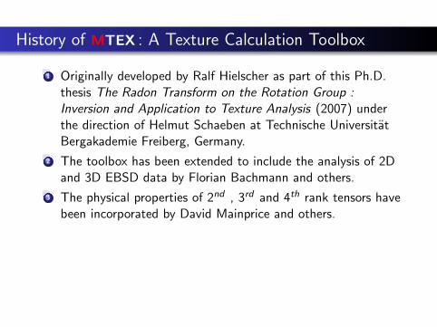
MATLAB programming style - Orientation tensor 2

The same Orientation tensor can also be formulated as asymmetric matrix and the product of the multiplication of a vectorcontaining all r by its transpose:

Mij =

M11 M12 M13

M12 M22 M23

M13 M23 M33

=1

N

N∑i

rTi ri

where r = (xi yi zi ) are direction cosines of a crystallographicdirection h in specimen coordinates r with Cartesian reference axesX, Y and Z.

MATLAB programming style - Orientation tensor 3

The two methods of calculation are illustrated by small MATLABscript. The method using the formation of covariance matrix froma column and row vector of r is 300 times faster. Efficientprogramming requires adapting to the MATLAB style.

MATLAB programming style - Orientation tensor 4

An example of c-axes pole figure of ice 1h at 1171m Talos Domeice core, Antarctica.

Eigen-vectors (red squares) : E1, E2, E3 Eigen-values (magnitudes) : EM1 > EM2 > EM3

G50 fabric analyser data courtesy of Maurine Montagnat LGGE UMR5183, CNRS / UJF Grenoble, France

Single Orientation Measurements in MTEX

Parameters of a single EBSD phase in MTEX

crystal symmetry

specimen symmetry

list of individual orientations

phase example olivine

arbitrary as list:

spatial coordinates x y

Band Contrast diffractionsignal

MAD Mean AngularDeviation

...Olivine in torsion: EBSD map data courtesy of Sylvie Demouchy,Montpellier

Colorcode for crystallographic directions

parallel to shear direction

Importing EBSD Data with The MTEX Import Wizard

Two ways to importEBSD data

1 From command window linkImport EBSD data

2 Type in the command window

import_wizard(’EBSD’)

Formats supported byMTEX :

*.ang TSL-EDAX

*.ctf HKL-Oxford

*.csv Oxford

*.sor LaboTEX

*.txt (Generic ASCII filesgenerated by user)

Importing EBSD Data - Using a script

This script was generated by the EBSD import wizard:

% C r y s t a l s y m m e t r i e s − d e f i n e a , b , c , a lpha , beta , gamma% and c r y s t a l d i r e c t i o n s used f o r E u l e r a n g l e C a r t e s i a n r e f e r e n c e frameCS = { . . .’ no t I ndexed ’ , . . .symmetry ( ’mmm’ , [ 4 . 7 5 6 10 .207 5 . 9 8 ] , ’ m i n e r a l ’ , ’ O l i v i n e ’ ) , . . .symmetry ( ’mmm’ , [ 1 8 . 2 4 0 6 8 .8302 5 . 1 8 5 2 ] , ’ m i n e r a l ’ , ’ E n s t a t i t e ’ ) , . . .symmetry ( ’ 2/m’ , [ 9 . 7 4 6 8 . 9 9 5 . 2 5 1 ] , [ 9 0 . 0 0 , 1 0 5 . 6 3 , 9 0 . 0 0 ]∗ degree , . . .’X | | a∗ ’ , ’Y | | b ’ , ’Z | | c ’ , ’ m i n e r a l ’ , ’ D i op s i d e ’ ) , . . .symmetry ( ’m−3m’ , ’ m i n e r a l ’ , ’ Magnet i t e ’ ) , . . .symmetry ( ’m−3m’ , ’ m i n e r a l ’ , ’ Chromite ’ )} ;% Specimen symmetrySS = symmetry ( ’−1 ’ ) ;

% path to f i l e spname = ’ /MatLab Programs/ ’% which f i l e s to be i m p o r t e dfname = { [ pname ’ 920D−13. c t f ’ ] ,}

% c r e a t e an EBSD v a r i a b l e c o n t a i n i n g t h e dataebsd = loadEBSD ( fname , CS , SS , ’ i n t e r f a c e ’ , ’ c t f ’ )

Visualize EBSD Data in MTEX : orientation space

Scatter plots in orientation space (Rodrigues space, axis-anglespace or Euler angle space)

% Not v e r y u s e f u l as a x e s a r e not l a b e l l e ds c a t t e r ( ebsd ( ’ O l i v i n e ’ ) , ’AXISANGLE ’ )s c a t t e r ( ebsd ( ’ O l i v i n e ’ ) , ’RODRIGUES ’ )

% More u s e f u l w i t h l a b e l l e d s e c t i o n sp l o t o d f ( ebsd ( ’ O l i v i n e ’ ) , ’ s igma ’ , ’SECTIONS ’ , 1 8 , ’ p o i n t s ’ ,320744)

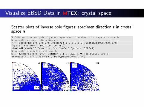
Visualize EBSD Data in MTEX : specimen space

Scatter plots of pole figures: crystal direction h in specimen space r

% O l i v i n e p o l e f i g u r e s% p l o t t i n g c o n v e n t i o n p l o t x 2 e a s t% X=East Y=North Z=C e n t e r upper h e m i s p h e r ep l o t x 2 e a s t

% s p e c i f y c r y s t a l d i r e c t i o n s h w i t h ’ h k l ’ f o r p o l e and ’ uvw ’ d i r e c t i o n sh = [ M i l l e r ( 1 , 0 , 0 , ’ uvw ’ ) , M i l l e r ( 0 , 1 , 0 , ’ uvw ’ ) , M i l l e r ( 0 , 0 , 1 , ’ uvw ’ ) ]f i g u r e ( ’ p o s i t i o n ’ , [ 1 0 0 100 700 3 5 0 ] )p l o t p d f ( ebsd ( ’ O l i v i n e ’ ) , h , ’ a n t i p o d a l ’ , ’ p o i n t s ’ ,320744)

% s p e c i f y spec imen d i r e c t i o n s r% you can used p r e d e f i n e d x v e c t o r , y v e c t o r o r z v e c t o r% o r d e f i n e a r b i t a r y d i r e c t i o n s w i t h v e c t o r 3 d ( 1 . 0 , 0 . 0 , 0 . 0 )r = [ v e c t o r 3 d ( 1 . 0 , 0 . 0 , 0 . 0 ) , v e c t o r 3 d ( 0 . 0 , 1 . 0 , 0 . 0 ) , v e c t o r 3 d ( 0 . 0 , 0 . 0 , 1 . 0 ) ]a n n o t a t e ( r , ’ a l l ’ , ’ l a b e l ’ ,{ ’X ’ , ’Y ’ , ’Z ’ } , ’ BackgroundColor ’ , ’w ’ )

Option : Antipodal (non-polar)

Option : Complete (polar)

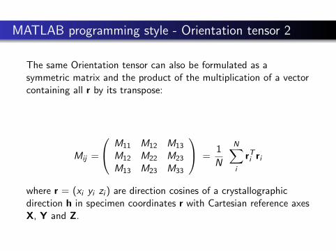
Visualize EBSD Data in MTEX : crystal space

Scatter plots of inverse pole figures: specimen direction r in crystalspace h% O l i v i n e i n v e r s e p o l e f i g u r e s : spec imen d i r e c t i o n r i n c r y s t a l s p a c e h% s p e c i f y spec imen d i r e c t i o n s rr = [ v e c t o r 3 d ( 1 . 0 , 0 . 0 , 0 . 0 ) , v e c t o r 3 d ( 0 . 0 , 1 . 0 , 0 . 0 ) , v e c t o r 3 d ( 0 . 0 , 0 . 0 , 1 . 0 ) ]f i g u r e ( ’ p o s i t i o n ’ , [ 1 0 0 100 700 3 5 0 ] )p l o t i p d f ( ebsd ( ’ O l i v i n e ’ ) , r , ’ a n t i p o d a l ’ , ’ p o i n t s ’ ,320744)

% s p e c i f y c r y s t a l d i r e c t i o n s hh = [ M i l l e r ( 1 , 0 , 0 , ’ uvw ’ ) , M i l l e r ( 0 , 1 , 0 , ’ uvw ’ ) , M i l l e r ( 0 , 0 , 1 , ’ uvw ’ ) ]a n n o t a t e ( h , ’ a l l ’ , ’ l a b e l e d ’ , ’ BackgroundColor ’ , ’w ’ )

Visualize EBSD Data in MTEX : Spatial maps

Spatial plots of EBSD data

% i p f o r i e n t a t i o n mapp l o t ( ebsd , ’ c o l o r c o d i n g ’ , ’ i p d f ’ )

% phase d i s t r i b u t i o n mapp l o t ( ebsd , ’ p r o p e r t y ’ , ’ phase ’ )

% d i f f r a c t e d i n t e n s i t y mapp l o t ( ebsd , ’ p r o p e r t y ’ , ’ bc ’ )

% mean a n g u l a r d e v i a t i o n e r r o r mapp l o t ( ebsd , ’ p r o p e r t y ’ , ’mad ’ )

Color Codings: ’bunge’,’angle’,’sigma’,’ihs’,

’ipdf’,’rodriguesquat’,

’rodriguesinverse’,’euler’,’bunge2’,’hkl’

Example hkl color coded orientation map

(Olivine torsion data courtesy of Sylvie Demouchy, GM, UM2, Montpellier)

Grain Analysis with MTEX

Grain reconstruction in MTEX is done via the commandcalcGrains. As an optional argument the desired threshold anglefor misorientation defining a grains boundary can be specified. Agrain is defined as a region, in which the misorientation of at leastone neighbouring measurement site is smaller than a giventhreshold angle. The command grainSize returns the number ofindexed pixels within a grain.% F i l l s a l l non i n d e x e d a r e a s . Angle i s t h e same f o r a l l p h a s e s .g r a i n s = c a l c G r a i n s ( ebsd , ’ a ng l e ’ ,10∗ degree ) ;

% Angle i s 0 ,10 & 15 f o r p h a s e s 1 , 2 , 3 . F i l l s a l l non i n d e x e d a r e a s .g r a i n s = c a l c G r a i n s ( ebsd , ’ a ng l e ’ , [ 0 10 5]∗ degree ) ;

% C o n s e r v e s non i n d e x e d a r e a s . Angle i s t h e same f o r a l l p h a s e s .g r a i n s = c a l c G r a i n s ( ebsd , ’ a ng l e ’ ,10∗ degree , ’ keepNot Indexed ’ ) ;

EBSD Map Grain Map : calcGrains(ebsd(’Olivine’),’angle’,10*degree)

Grain Properties

EBSD properties

p lot ( g r a i n s ) % p l o t a l l g r a i n sp lot ( g r a i n s ( ’ O l i v i n e ’ ) % p l o t o l i v i n e g r a i n sp lot ( g r a i n s , ’ p r o p e r t y ’ , ’ phase ’ ) % p l o t t he phase o f each g r a i np l o t B o u n d a r y ( g r a i n s ) % p l o t g r a i n b o u n d a r i e s

Plot grain boundaries:

p l o t b o u n d a r y ( g r a i n s ,/+<op t i o n s>+/)p l o t b o u n d a r y ( g r a i n s , ’ p r o p e r t y ’ , ’ a ng l e ’ )p l o t b o u n d a r y ( g r a i n s , ’ p r o p e r t y ’ , r o t )

Access to properties of grains

phase = get ( g r a i n s , ’ phase ’ )g r a i n s q u a r t z = g r a i n s ( ’ Quartz ’ )o = get ( g r a i n s q u a r t z , ’ o r i e n t a t i o n ’ )

Grain Properties

EBSD properties

p lot ( g r a i n s ,/+<op t i o n s>+/)/+p lot ( g r a i n s , ’ p r o p e r t y ’ , phase ’ )+/

Plot grain boundaries:

p l o t b o u n d a r y ( g r a i n s ,/+<op t i o n s>+/)p l o t b o u n d a r y ( g r a i n s , ’ p r o p e r t y ’ , ’ a ng l e ’ )p l o t b o u n d a r y ( g r a i n s , ’ p r o p e r t y ’ , r o t )

Access to properties of grains

phase = get ( g r a i n s , ’ phase ’ )g r a i n s q u a r t z = g r a i n s ( ’ Quartz ’ )o = get ( g r a i n s q u a r t z , ’ o r i e n t a t i o n ’ )

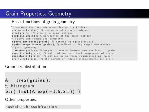
Grain Properties: Geometry

Basic functions of grain geometry% commands t h a t i n c l u d e non−i n d e x p o i n t s ( h o l e s )p e r i m e t e r ( g r a i n s ) ; % p e r i m e t e r o f a g r a i n−p o l y g o na r e a ( g r a i n s ) ; % a r e a o f a g r a i n−p o l y g o nc e n t r o i d ( g r a i n s ) ; % b a r y c e n t e r o f t h e g r a i n−p o l y g o n

% e q u i v a l e n t r a d i u s and p e r i m e t e re q u i v a l e n t r a d i u s ( g r a i n s ) ; % d e f i n e d as s q r t ( a r e a / p i )e q u i v a l e n t p e r i m e t e r ( g r a i n s ) ; % d e f i n e d as 2∗ p i∗ e q u i v a l e n t r a d i u s

% g r a i n geometryd i a m e t e r ( g r a i n s ) ; % l o n g e s t d i s t a n c e between two v e r t i c e s o f g r a i na s p e c t r a t i o ( g r a i n s ) ; % r a t i o o f two p r i n c i p a l components o f a g r a i ns h a p e f a c t o r ( g r a i n s ) ; % d e f i n e d as p e r i m e t e r / e q u i v a l e n t p e r i m e t e rg r a i n S i z e ( g r a i n s ) ; % t h e number o f i n d e x e d measurements p e r g r a i n

Grain-size distribution

A = a r e a ( g r a i n s ) ;% h i s t o g r a mbar ( h i s t (A, exp ( −1 . 5 : 6 . 5 ) ) )

Other properties:

h a s h o l e s , h a s s u b f r a c t i o n

Selecting grains after properties

s e l e c t e d g r a i n s = g r a i n s ( g r a i n S i z e ( g r a i n s ) > 10)l a r g e g r a i n s = g r a i n s ( p e r i m e t e r ( g r a i n s ) > 150| s e l e c t e d g r a i n s )

Working with EBSD Data Directly

Access EBSD properties

o r i e n t a t i o n s = get ( ebsd , ’ o r i e n t a t i o n ’ )x = get ( ebsd , ’ x ’ )

Rotate EBSD data

ebsd = rotate ( ebsd , r o t a t i o n ( . . .’ a x i s ’ , xvector , ’ a ng l e ’ ,90∗ degree ) )

Omit one pixel grains

% g r a i n s c o n t a i n i n g more than one i n d e x e d p i x e lg r a i n s = g r a i n s ( g r a i n s i z e ( g r a i n s ) > 1)

EBSD to ODF Reconstruction in MTEX

MTEX uses kernel density estimation to compute an ODF fromEBSD data. The sensitive parameter of this method is the kernelfunction.

Syntax:

od f = calcODF ( ebsd ,<op t i o n s>)

Options:

’ k e r n e l ’ % th e k e r n e l to be used’ h a l f w i d t h ’ % h a l f−width o f t he k e r n e l’ r e s o l u t i o n ’ % r e s o l u t i o n o f a p p r o x i m a t i o n g r i d’ F o u r i e r ’ % ODF by i t s F o u r i e r c o e f f i c i e n t s’ e x a c t ’ % e x a c t g r i d