FEATURES OF SLEEP APNEA RECOGNITION AND …s2is.org/Issues/v7/n2/papers/paper3.pdf · Obstructive...

FEATURES OF SLEEP APNEA RECOGNITION AND ANALYSIS

LEONG WAI YIE, JOEL THAN CHIA MING

Taylor’s University, Lakeside Campus, No.1, Jalan Taylor’s, 47500 Subang Jaya, Selangor

Emails: [email protected]

Submitted: Feb. 15, 2014 Accepted: May 2, 2014 Published: June 1, 2014

Abstract- Sleep apnea is a growing sleep disorder issue and estimate to affect 7% of the adult population in

Malaysia. In this study, the electrical activity of the brain is studied using Electroencephalogram (EEG).

The data obtained was then decomposed using three methods; Empirical Mode Decomposition (EMD),

Bivariate EMD and finally Ensemble EMD. The Index of Orthogonatility (IO) was obtained which shows

EMD performed the most poorly, EEMD the best and Bivariate in between. The performance of EMD

greatly improves when the number of samples was greatly decreased and very high peaks and more complex

parts of the signal were excluded in the analysis. Segmentation was also conducted and the segmentation

error revealed when an Event Related Potential (ERP) has happened which is when apnea occurred.

Index terms: Sleep apnea, Electroencephalogram (EEG), Empirical Mode Decomposition (EMD), Bivariate

EMD, Ensemble EMD

INTERNATIONAL JOURNAL ON SMART SENSING AND INTELLIGENT SYSTEMS VOL. 7, NO. 2, JUNE 2014

481

I. INTRODUCTION

Obstructive sleep apnea syndrome (OSAS) is a problem that involves two factors which are

anatomical and neurological factors[1]. OSAS is characterised primarily by periodic collapses of the

upper airway during sleep which contributes the main characteristic of the disease [2]. The airway

calibre is smaller in the apneic compared to a normal subject. It is also noticeable that the soft palate

and tongue area are larger in the apneic [2]. This problem leading to either complete or partial

obstruction of the airway, will result in apneas, hypopneas, or both. This disorder causes daytime

sleepiness, neurocognitive defects, and depression. It affects almost every system in the body,

resulting in an increased incidence of hypertension, cardiovascular disease, stroke, pulmonary

hypertension, cardiac arrhythmias, and altered immune function. It also increases the risk of having

an accident, presumably as a result of associated somnolence [3].

It is estimated 7% of the adult population or 1.9 million people in Malaysia are affected by

OSA [4]. The gold standard for the diagnosis of sleep apnea is an overnight polysomnogram. Split-

night studies are becoming increasingly common and allow for quicker implementation of therapy at

a reduced cost. Treatment options for sleep apnea include weight loss, positional therapy, oral

devices, continuous positive airway pressure (CPAP), and upper airway surgery. One of the major

components of PSG is the Electroencephalogram (EEG). EEG is able to pick up different electrical

brain activities. The first recording of the electric field of the human brain was made by the German

psychiatrist Hans Berger in 1924 in Jena. He gave this recording the name electroencephalogram

(EEG). EEG measures namely three kinds of activity which are spontaneous activity, evoked

potentials, and bioelectric events produced by single neurons [5].

In this study, 10-20 international electrode placement system is used. In this system, 21

electrodes are located on the surface of the scalp, as shown in Figure 1.1. The positions are

determined from the reference points, which is the delve at the top of the nose, level with the eyes;

and inion, which is the bony lump at the base of the skull on the midline at the back of the head.

From these points, the skull perimeters are measured in the transverse and median planes. Electrode

locations are determined by dividing these perimeters into 10% and 20% intervals. Three other

electrodes are placed on each side equidistant from the neighbouring points, as shown in Figure 1.2

[5].

LEONG WAI YIE, JOEL THAN CHIA MING, FEATURES OF SLEEP APNEA RECOGNITION AND ANALYSIS

482

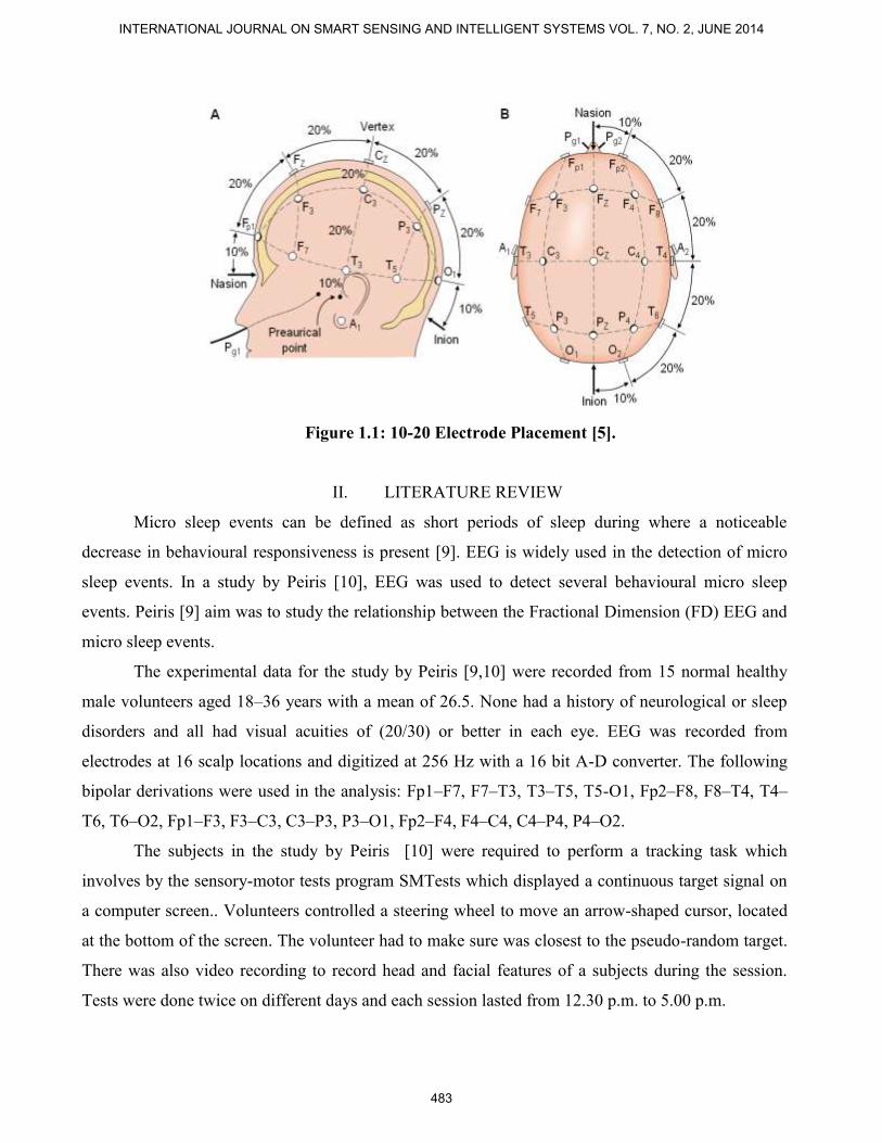
Figure 1.1: 10-20 Electrode Placement [5].

II. LITERATURE REVIEW

Micro sleep events can be defined as short periods of sleep during where a noticeable

decrease in behavioural responsiveness is present [9]. EEG is widely used in the detection of micro

sleep events. In a study by Peiris [10], EEG was used to detect several behavioural micro sleep

events. Peiris [9] aim was to study the relationship between the Fractional Dimension (FD) EEG and

micro sleep events.

The experimental data for the study by Peiris [9,10] were recorded from 15 normal healthy

male volunteers aged 18–36 years with a mean of 26.5. None had a history of neurological or sleep

disorders and all had visual acuities of (20/30) or better in each eye. EEG was recorded from

electrodes at 16 scalp locations and digitized at 256 Hz with a 16 bit A-D converter. The following

bipolar derivations were used in the analysis: Fp1–F7, F7–T3, T3–T5, T5-O1, Fp2–F8, F8–T4, T4–

T6, T6–O2, Fp1–F3, F3–C3, C3–P3, P3–O1, Fp2–F4, F4–C4, C4–P4, P4–O2.

The subjects in the study by Peiris [10] were required to perform a tracking task which

involves by the sensory-motor tests program SMTests which displayed a continuous target signal on

a computer screen.. Volunteers controlled a steering wheel to move an arrow-shaped cursor, located

at the bottom of the screen. The volunteer had to make sure was closest to the pseudo-random target.

There was also video recording to record head and facial features of a subjects during the session.

Tests were done twice on different days and each session lasted from 12.30 p.m. to 5.00 p.m.


483

EEG was also used in a system developed to detect micro sleep events. The study in a study

by [11,14-21] developed a system integrating EEG features as well as other features causing a feature

fusion to detect sleep events. The feature fusion includes brain electric activity, variation in the pupil

size, and eye and eyelid movements.

Figure Error! No text of specified style in document.1: Driving Simulation Setup[11].

The test subjects in [11] were 23 young adults started driving in s real car driving simulation

lab (Fig. 2.1) at 1:00 A.M. after a day of normal activity and where there must be nonstop 16 hours of

sleeplessness. The subjects had to accomplish seven driving sessions lasting 40 min, each followed

by a 15 min long period of responding to sleepiness questionnaires and of vigilance tests and of a 5

min long break. The driving tasks were chosen intentionally monotonous to support drowsiness and

occurrence of micro sleep events.

III. METHODOLOGY

Empirical Mode Decomposition (EMD) was introduced by Huang [6] for analysing nonlinear and

non-stationary data. EMD processes complicated data set and decomposes into a finite number of

`intrinsic mode functions' (IMF) that can further processed with Hilbert transforms. This method is

adaptive and efficient where parameters can be changed according to the user. This method can

process nonlinear and non-stationary processes. EEG data can be non-linear and non-stationary

initially used for ocean wave signals it has found more and more interest in biomedical engineering

[7].

Original raw data can be expressed as an equation following [6]:

x(t) = s(t) + n(t) (3.1)

1. Digital polygraphy PC

2. Eyetracing system PC

3. Experiment control PC

4. Video capture PC

5. Driving simulation PC & online

questionnaires

6. Multi camera unit of the eye-tracing system

7. Recording of steering angle & lane deviation

8. Polygraphy head box

9. Video projector

10. Real car (GM Opel “Corsa”)

11. Digital video camera

12. Projection area

13. Loudspeaker

14. Microphone


484

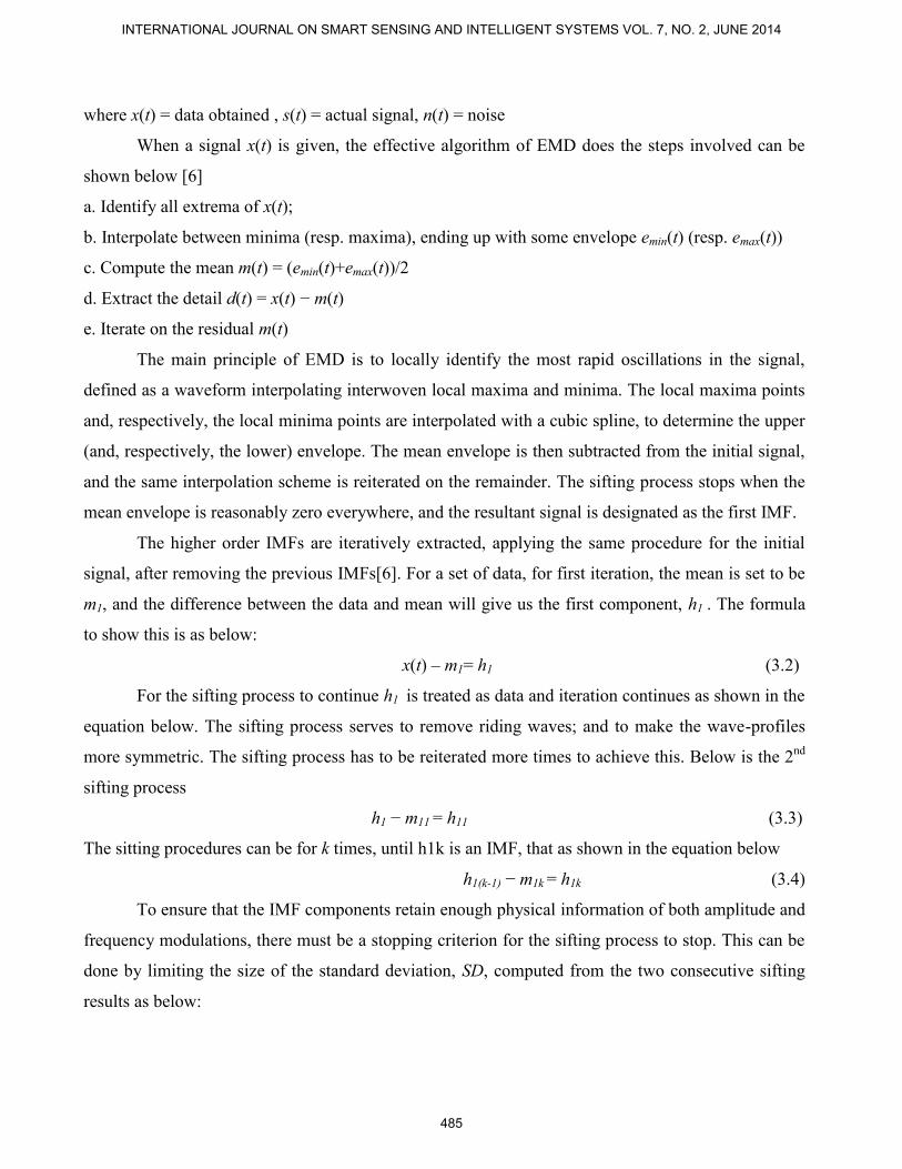
where x(t) = data obtained , s(t) = actual signal, n(t) = noise

When a signal x(t) is given, the effective algorithm of EMD does the steps involved can be

shown below [6]

a. Identify all extrema of x(t);

b. Interpolate between minima (resp. maxima), ending up with some envelope emin(t) (resp. emax(t))

c. Compute the mean m(t) = (emin(t)+emax(t))/2

d. Extract the detail d(t) = x(t) − m(t)

e. Iterate on the residual m(t)

The main principle of EMD is to locally identify the most rapid oscillations in the signal,

defined as a waveform interpolating interwoven local maxima and minima. The local maxima points

and, respectively, the local minima points are interpolated with a cubic spline, to determine the upper

(and, respectively, the lower) envelope. The mean envelope is then subtracted from the initial signal,

and the same interpolation scheme is reiterated on the remainder. The sifting process stops when the

mean envelope is reasonably zero everywhere, and the resultant signal is designated as the first IMF.

The higher order IMFs are iteratively extracted, applying the same procedure for the initial

signal, after removing the previous IMFs[6]. For a set of data, for first iteration, the mean is set to be

m1, and the difference between the data and mean will give us the first component, h1 . The formula

to show this is as below:

x(t) – m1= h1 (3.2)

For the sifting process to continue h1 is treated as data and iteration continues as shown in the

equation below. The sifting process serves to remove riding waves; and to make the wave-profiles

more symmetric. The sifting process has to be reiterated more times to achieve this. Below is the 2nd

sifting process

h1 − m11 = h11 (3.3)

The sitting procedures can be for k times, until h1k is an IMF, that as shown in the equation below

h1(k-1) − m1k = h1k (3.4)

To ensure that the IMF components retain enough physical information of both amplitude and

frequency modulations, there must be a stopping criterion for the sifting process to stop. This can be

done by limiting the size of the standard deviation, SD, computed from the two consecutive sifting

results as below:


485

(3.5)

The SD is usually set to be between 0.2 and 0.3. This is a very rigorous limitation for the

difference between siftings. Huang [6] did a comparison and found that Fourier spectra, computed by

shifting of only five out of 1024 points from the same data, can have an equivalent SD of 0.2-0.3

calculated point-by-point.

With any stoppage criterion, the c1 should contain the finest scale or the shortest period

component of the signal. This is to allow the c1 to be removed from the rest of the data by [6].

x(t) – c1 = r1 (3.6)

This gives the residue r1 which contains all longer period variations in the data, it will become

as new data and it is sifted, giving r2 as shown below.

r1 – c1=r2 (3.7)

The repeated processes will continue and expressed as below [6]

r(n−1) – cn = rn (3.8)

By summing up, the equation below is obtained (Huang, 1998a);

(3.9)

IV. EXPERIMENTAL SETUP

Figure 4.1 shows various stages involved in the entire experiment. The first stage of Data Acquisition

involves the usage of EEG and test subjects to obtain the right data. It involves the preparation of the

subject and placing of electrodes. The venue should be in a comfortable area to allow the subject to

sleep and not be anxious. The second stage involves processing the data using different methods,

EMD [6], EEMD [12] and Bivariate EMD [13]. Further processing can be done to see the

effectiveness of the methods. Finally the third stage is the analysis of the processed data to identify

characteristics of sleep apnea. This is where the features of sleep and sleep apnea are identified. The

differences between each method are also determined.

Figure 4.1 Data Acquisition using Actiwave EEG

ST

AR

T

Preparation

of subjects

Electrode

Placement

C3, C4, O1,

O2 & A1

Subject

allowed to

relax for

15min

Subject

allowed to

sleep for 1

hour

After 1 hour

sleep, EEG

removed

Data Sent

for

Processing


486

The Actiwave EEG is a miniature biomedical waveform recorders are designed to capture

EMG, EEG and ECG signals in daily living. Using miniatures recorders, EMG, EEG and ECG

waveforms can be recorded discreetly without the need for a large belt mounted recorder or lengthy

wires. Each recorder can be taped or glued to the skin near to the position of the electrodes. The very

small size and weight of these units makes them ideal for paediatric and veterinary use. In this

experiment it was chosen because of its mobility allowing the test subject to be practically anywhere

to obtained the data and would not be restricted to the laboratory. It is quite versatile because of its

maximum 13 hours of recording. It fully recharges in 4 hours and has non-volatile memory.

Firstly, the specific areas for electrode placed was marked by skin marker and cleaned by

abrasive skin preparation gel called test subject preparation. Then, the adhesive and conductive paste

was used to attach the electrode onto scalp. The electrode was secured also by adhesive tape. The test

subject was advised not to consume any stimulants or depressants, such as alcohol, caffeine, and

nicotine, during the 4 hours prior to the session. Also test subjects were asked to relax themselves as

usual when they attempted to sleep as done in studies before.

Electrodes which detect the signal should place it according to the 10-20 electrode

international placement system as shows in Figure 1.2. Electrodes were place in position C3, C4, O1,

O2 and A1 were recorded by the CamNtech Actiwave EEG. The CamNtech Actiwave 4-channel

Recorder (Figure 4.2) was used to collect and record the EEG signal. CamNtech Actiwave Interface

Dock is used as the interface for the EEG recorder and the computer. Embedded system in the EEG

device has a feature filter undesirable noise and interference from the environment to provide more

accurate and precise results for clinicians and researchers to carry out the analysis.

The C3 and C4 locations were chosen because these regions are where electrical activity in

somato-sensoric and motoric brain areas can be picked up. O1 and O2 are related to the primary and

secondary visual areas to detect Rapid Eye Movement. A1 is serves as the reference electrode so that

all the other electrodes can be referenced with. The EEG was sampled at 260 Hz.

Figure 4.2: Devices and materials that used during experiment.

The devices consist of as below:

(1) Adhesive and conductive paste.

(2) Abrasive skin prepping gel.

(3) Medical Tape.

(4) CamNtech Actiwave Interface Dock.

(5) Gold plate electrodes.

(6) CamNtech Actiwave 4-channel recorder.


487

Data acquired from Actiwave EEG alone will limit the research capabilities and the outcome

of this research. This is because Actiwave EEG only records just the EEG. A complete

polysomnogram includes blood oxygen measurement, sound measurement as well as

Electrocardiogram. With the limited materials this study was held to get a more extensive data.

Therefore Actiwave EEG was used to measure EEG only if a person is normal.

Since a sleep study lasts for a few hours, the steps involved; processing the whole data of

sleep followed selecting the data would be too time consuming. So this study looked for areas where

there was a drop in oxygen level. A drop in oxygen level would indicate that an apnea might have

happened. The second indicator would be to see if there are rises in sound level. Rises in sound level

would indicate snoring or difficulty in bringing also another characteristic of apnea. After this two

indicators are matched then the EEG timing is noted and the portion of EEG is then extracted for

analysis.

V. RESULTS AND DISCUSSIONS

5.1 Comparison of Index of Orthogonatility

The data which is 1500 time samples from C3 channel sampled at 256 Hz was ran on all 3 algorithms

EMD, EEMD, and Bivariate giving the values of Index of Orthogatility as below:

Table 5.1: Index of Orthogonatility for different decompositions

Decomposition Method Index of Orthogonatility

EMD 0.2579

EEMD 0.1989

Bivariate EMD 0.2026

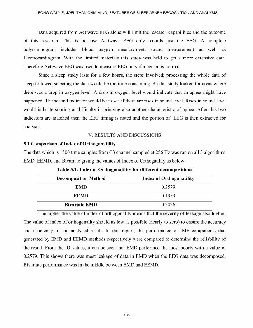
The higher the value of index of orthogonality means that the severity of leakage also higher.

The value of index of orthogonality should as low as possible (nearly to zero) to ensure the accuracy

and efficiency of the analysed result. In this report, the performance of IMF components that

generated by EMD and EEMD methods respectively were compared to determine the reliability of

the result. From the IO values, it can be seen that EMD performed the most poorly with a value of

0.2579. This shows there was most leakage of data in EMD when the EEG data was decomposed.

Bivariate performance was in the middle between EMD and EEMD.


488

5.2 Comparison of IMFs

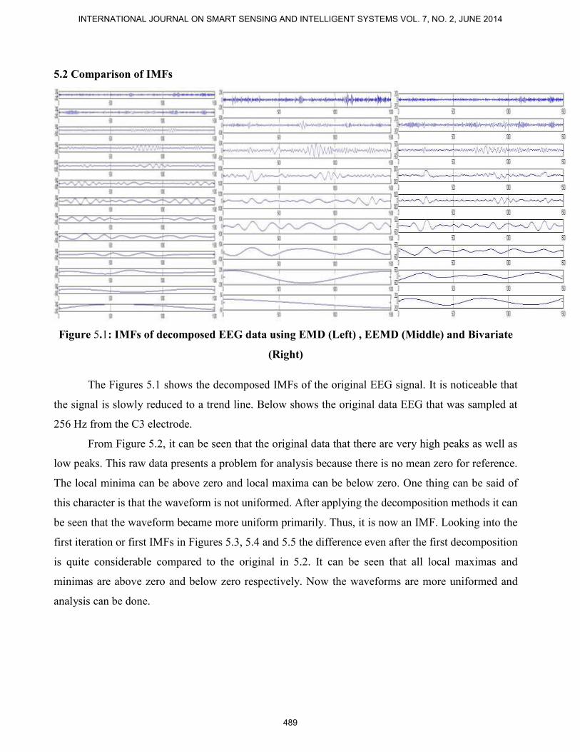
Figure 5.1: IMFs of decomposed EEG data using EMD (Left) , EEMD (Middle) and Bivariate

(Right)

The Figures 5.1 shows the decomposed IMFs of the original EEG signal. It is noticeable that

the signal is slowly reduced to a trend line. Below shows the original data EEG that was sampled at

256 Hz from the C3 electrode.

From Figure 5.2, it can be seen that the original data that there are very high peaks as well as

low peaks. This raw data presents a problem for analysis because there is no mean zero for reference.

The local minima can be above zero and local maxima can be below zero. One thing can be said of

this character is that the waveform is not uniformed. After applying the decomposition methods it can

be seen that the waveform became more uniform primarily. Thus, it is now an IMF. Looking into the

first iteration or first IMFs in Figures 5.3, 5.4 and 5.5 the difference even after the first decomposition

is quite considerable compared to the original in 5.2. It can be seen that all local maximas and

minimas are above zero and below zero respectively. Now the waveforms are more uniformed and

analysis can be done.


489

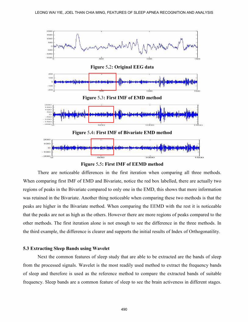
Figure 5.2: Original EEG data

Figure 5.3: First IMF of EMD method

Figure 5.4: First IMF of Bivariate EMD method

Figure 5.5: First IMF of EEMD method

There are noticeable differences in the first iteration when comparing all three methods.

When comparing first IMF of EMD and Bivariate, notice the red box labelled, there are actually two

regions of peaks in the Bivariate compared to only one in the EMD, this shows that more information

was retained in the Bivariate. Another thing noticeable when comparing these two methods is that the

peaks are higher in the Bivariate method. When comparing the EEMD with the rest it is noticeable

that the peaks are not as high as the others. However there are more regions of peaks compared to the

other methods. The first iteration alone is not enough to see the difference in the three methods. In

the third example, the difference is clearer and supports the initial results of Index of Orthogonatility.

5.3 Extracting Sleep Bands using Wavelet

Next the common features of sleep study that are able to be extracted are the bands of sleep

from the processed signals. Wavelet is the most readily used method to extract the frequency bands

of sleep and therefore is used as the reference method to compare the extracted bands of suitable

frequency. Sleep bands are a common feature of sleep to see the brain activeness in different stages.


490

Figure 5.6 shows all the five bands that could be extracted from the same original EEG data using

Wavelet transformation.

Figure 5.6: Frequency bands of Sleep using Wavelet Method:

(a) Gamma (b) Beta (c) Alpha (d) Theta (e) Delta

Table 5.2: Decrease of Frequency using EMD

Frequency (Hz)

IMF EMD Band

1st 42.66666667 Gamma

2nd

23.48751357 Beta

3rd

13.34201954 Alpha

4th

7.852334419 Theta

5th

4.447339848 Delta

6th

2.640608035 Delta

7th

1.667752443 Delta

8th

0.833876221 Delta

9th

0.555917481 Delta

10th

0.347448426 Delta

11th

0.208469055 Delta

12th

0.13897937 Delta

13th

0.13897937 Delta

14th

0.069489685 Delta


491

The wavelet transforms the frequency of the original signal into half and each transform

further transform into another half. Therefore since the frequency is 128 Hz using wavelet, the

frequency is transformed from 128Hz to 64Hz for Gamma band, 64 to 32Hz Beta band, 32Hz to

16Hz for Alpha band and 16Hz to 8Hz for Theta band. The delta band is obtained reconstructing

from the coefficients of the theta band which is the fourth level of decomposition. Therefore four

levels of decomposition is only needed to obtain the five bands Figure 5.6.

5.4 Extracting Sleep Bands using EMD

Unlike wavelet, EMD, Bivariate and EEMD approach to finding the sleep bands are not as

straightforward as the wavelet. This is because the underlying principle of decomposition of these

three methods is different than wavelet. The frequency after each level of decomposition changes not

in a fixed rate of halves as the Wavelet method. The frequency definitely decreases after

decomposition. However the decrease is usually less than half the frequency therefore it cannot

straightaway be utilised for all levels of decomposition for the energy bands as in wavelet method.

The first method is to determine the frequency of all IMFs of each method. Another constraint is that

since there is no fixed numbers of IMFs per method therefore the parameters of frequency have to be

changed when changing data. Therefore the frequency of each IMF must be evaluated to see how

they can be represented into energy bands.

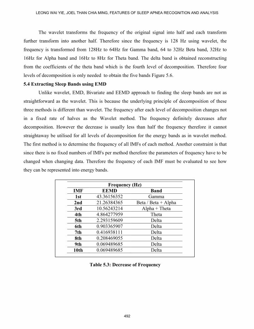
Table 5.3: Decrease of Frequency

Frequency (Hz)

IMF EEMD Band

1st 43.36156352 Gamma

2nd 21.26384365 Beta / Beta + Alpha

3rd 10.56243214 Alpha + Theta

4th 4.864277959 Theta

5th 2.293159609 Delta

6th 0.903365907 Delta

7th 0.416938111 Delta

8th 0.208469055 Delta

9th 0.069489685 Delta

10th 0.069489685 Delta


492

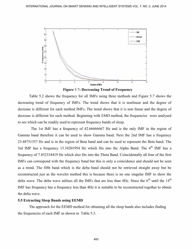
Figure 5.7: Decreasing Trend of Frequency

Table 5.2 shows the frequency for all IMFs using three methods and Figure 5.7 shows the

decreasing trend of frequency of IMFs. The trend shows that it is nonlinear and the degree of

decrease is different for each method IMFs. The trend shows that it is non linear and the degree of

decrease is different for each method. Beginning with EMD method, the frequencies were analysed

to see which can be readily used to represent frequency bands of sleep.

The 1st IMF has a frequency of 42.66666667 Hz and is the only IMF in the region of

Gamma band therefore it can be used to show Gamma band. Next the 2nd IMF has a frequency

23.48751357 Hz and is in the region of Beta band and can be used to represent the Beta band. The

3rd IMF has a frequency 13.34201954 Hz which fits into the Alpha Band. The 4th

IMF has a

frequency of 7.852334419 Hz which also fits into the Theta Band. Coincidentally all four of the first

IMFs can correspond with the frequency band but this is only a coincidence and should not be seen

as a trend. The fifth band which is the delta band should not be retrieved straight away but be

reconstructed just as the wavelet method this is because there is no one singular IMF to show the

delta wave. The delta wave utilises all the IMFs that are less than 4Hz. Since the 6th

until the 14th

IMF has frequency has a frequency less than 4Hz it is suitable to be reconstructed together to obtain

the delta wave.

5.5 Extracting Sleep Bands using EEMD

The approach for the EEMD method for obtaining all the sleep bands also includes finding

the frequencies of each IMF as shown in Table 5.3.


493

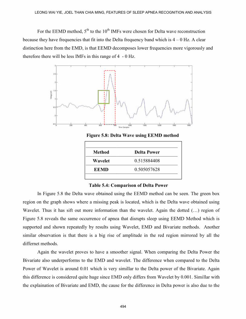
For the EEMD method, 5th

to the 10th

IMFs were chosen for Delta wave reconstruction

because they have frequencies that fit into the Delta frequency band which is 4 – 0 Hz. A clear

distinction here from the EMD, is that EEMD decomposes lower frequencies more vigorously and

therefore there will be less IMFs in this range of 4 - 0 Hz.

Figure 5.8: Delta Wave using EEMD method

Table 5.4: Comparison of Delta Power

In Figure 5.8 the Delta wave obtained using the EEMD method can be seen. The green box

region on the graph shows where a missing peak is located, which is the Delta wave obtained using

Wavelet. Thus it has sift out more information than the wavelet. Again the dotted (…) region of

Figure 5.8 reveals the same occurrence of apnea that disrupts sleep using EEMD Method which is

supported and shown repeatedly by results using Wavelet, EMD and Bivariate methods. Another

similar observation is that there is a big rise of amplitude in the red region mirrored by all the

differnet methods.

Again the wavelet proves to have a smoother signal. When comparing the Delta Power the

Bivariate also underperforms to the EMD and wavelet. The difference when compared to the Delta

Power of Wavelet is around 0.01 which is very simillar to the Delta power of the Bivariate. Again

this difference is considered quite huge since EMD only differs from Wavelet by 0.001. Simillar with

the explaination of Bivariate and EMD, the cause for the difference in Delta power is also due to the

Method Delta Power

Wavelet 0.515884408

EEMD 0.505057628


494

limited number of IMFs used to reconstruct the Delta wave as seen in the Bivariate method. In the

EMD method used 9 IMFs to reconstruct the Delta wave where as for the EEMD method, it used

only 6 IMFs to reconstruct the delta wave. Since less IMFs are used, there are less sources to

reconstruct. This results a loss in information for the Delta wave. Therefore this supports the notion

that having more IMFs when used to reconstruct would produce more accurate reconstructions

especially in the Delta wave and Delta power.

Thus it is important to have more IMFs to achieve the highest similarity of Delta wave if

compared to the wavelet method. This can be a constraint especially when there are no more IMFs

and the decomposition method decomposes vigorously IMFs of lower frequencies.

VI. CONCLUSIONS

In this study, signal processing using EMD, EEMD and bivariate EMD were analysed on

EEG data from a sleep apnea patient. The milestone achieved is in comparing the index of

Orthogonality, instantaneous frequency, amplitudes, energy and sleep bands of all 3 methods. This

report shows the general view that Bivariate EMD is better than EMD however not as good as

EEMD. All three methods manage to show certain features regarding the sleep data that were

meaningful. All three methods manage to show the occurrence of apnea, sleep bands, correlation with

sound waves as well as delta power. All three methods are effective in showing that apnea has

happened. The Bivariate is more favourable is looking at the data as a whole, where as EEMD is

more favourable if looking at specific IMFs and the EMD is more favourable especially at looking at

Delta power only.

There are few major challenges faced for this project. The first is obtaining the data for all

sleep apnea patients. This is quite a laborious task because effort and time needs to be taken to find

these patients to obtain proper data. The conditions of obtaining the data must also be constant so that

the results have the same constraints and may not be affected by changing environments. The second

challenge would be in detecting the key features of the EEG data because EEG data are usually

interpreted. Therefore, time and care needs to be taken to learn to interpret the EEG data.

To improve, firstly there must be a set up of a control experiment in order to compare results

obtained. The control experiment must be independent of the variables that contribute to sleep apnea

detection. For example, subjects who are female have less probability to have sleep apnea whereas


495

subjects with obesity have very high probability to have sleep apnea. Therefore the subjects chosen

for the control experiment must be chosen carefully.

REFERENCES

[1] Pack, A. I., 2002. Sleep Apnea: Pathogenesis, Diagnosis and Treatment. 1st ed. s.l.:CRC Press.

[2] Tung, R. and Leong, W.Y, 2013, Processing obstructive sleep apnea syndrome (OSAS) data.

Journal of Biomedical Science and Engineering, 6, 152-164. doi: 10.4236/jbise.2013.62019.

[3] Caples, S. M., Gami, A. S., & Somers, V. K., 2005. Obstructive sleep apnea. Annals of internal

medicine, 142(3), pp. 187-197.

[4] TheStar Publications, 2011. Sleep Well.

[5] Harrison, Y., & Horne, J. A., 1996. Occurrence of 'microsleeps' during daytime sleep onset in

normal subjects. Electroencephalogr. Clin. Neurophysiol., Volume 98, pp. 411-416.

[6] Huang, N. E. et al., 1998a. The empirical mode decomposition and the Hilbert spectrum for

nonlinear and nonstationary time series analysis. Proceedings of the Royal Society of London.

Series A: Mathematical, Physical and Engineering Sciences, 454(1971), pp. 903–995.

[7] Huang, W. et al., 1998b. Engineering analysis of biological variables: an example of blood

pressure over 1 day. Proceedings of the National Academy of Sciences,, 95(9), pp. 4816-4821.

[8] Golz, M. et al., 2007. Feature Fusion for the Detection of Microsleep Events. Journal of VLSI

Signal Processing, Vol.49, pp.329-342.

[9] Peiris, M. T. R. et al., 2006a. Detecting behavioral microsleeps from EEG power spectra.

Engineering in Medicine and Biology Society, 2006. EMBS'06. 28th Annual International

Conference of the IEEE, p. 5723.

[10] Peiris, M.T.R. et al., 2006b. Fractal dimension of the EEG for detection of behavioural

microsleeps. Shanghai, IEEE, pp.5742-5745.

[11] Poudel, Govinda R., et al., 2010. The Relationship Between Behavioural Microsleeps,

Visuomotor Performance and EEG Theta. Bueno Aires, IEEE, pp. 4452-4455.

[12] Rilling, G. et al., 2007. Bivariate empirical mode decomposition. Signal Processing Letters

IEEE, 14(12), p. 9360939.

[13] Wu, Z., & Huang, N. E., 2009. Ensemble empirical mode decomposition: A noise-assisted

data analysis method. Advances in Adaptive Data Analysis, 1(1), pp. 1-41.


496

[14] Leong W.Y,, Mandic D.P., Liu W., 2007, Blind Extraction of Noisy Events Using Nonlinear

Predictor, ICASSP 2007, IEEE, Pages:657-670, 1520-6149.

[15] Leong W.Y., Homer J., 2004, Implementing ICA in blind multiuser detection, IEEE

International Symposium on Communications and Information Technology (ISCIT) 2004., Vol.2,

pp.947-952.

[16] Leong WY, Mandic DP, M Golz, D Sommer, 2007, Blind extraction of microsleep events,

15th International Conference on Digital Signal Processing, pp.207-210.

[17] Leong WY, 2006, Implementing Blind Source Separation in Signal Processing and

Telecommunications, PhD Thesis, The University of Queensland.

[18] Leong WY, Mandic DP 2007, Noisy component extraction (noice), IEEE International

Symposium on Circuits and Systems, IEEE, Pages:3243-3246.

[19] E. B. Tan, D. and Leong, W. (2012) Sleep disorder detection and identification. Journal of

Biomedical Science and Engineering, 5, 330-340. doi: 10.4236/jbise.2012.56043.

[20] B. Ginzburg, L. Frumkis, B.Z. Kaplan, A. Sheinker, and N. Salomonski, 2008, Investigation Of

Advanced Data Processing Technique In Magnetic Anomaly Detection Systems, International

Journal On Smart Sensing and Intelligent Systems, Inaugural Issue

VOL. 1, NO. 1, MARCH 2008, Pages: 110-122.

[21] Xu Xiaobin, Zhou Zhe, Wen Chenglin, Data Fusion Algorithm of Fault Diagnosis Considering

Sensor Measurement Uncertainty, International Journal On Smart Sensing and Intelligent

Systems, VOL. 6, NO. 1, FEB 2013, Pages: 171 – 190.


497

FEATURES OF SLEEP APNEA RECOGNITION AND …s2is.org/Issues/v7/n2/papers/paper3.pdf · Obstructive...

Documents

Transcript of FEATURES OF SLEEP APNEA RECOGNITION AND …s2is.org/Issues/v7/n2/papers/paper3.pdf · Obstructive...