
Feature selection - asc.ohio-state.edu
30
Feature selection Micha Elsner January 29, 2014
Transcript of Feature selection - asc.ohio-state.edu

Feature selection
Micha Elsner
January 29, 2014

Using megam as max-ent learnerI Hal Daume III from UMD wrote a max-ent learnerI Pretty typical of many classifiers out there...
Step one: create a text file with tags and features:IN word-In title-caseDT word-anNNP has-punc title-case word-Oct. mixed-caseCD numeric word-19<TAG> <feature> <feature> <feature>
I Features are binary; only write down those with value 1
Step two: run megamI multitron selects stochastic gradient training
megam_i686.opt -nc -pa multitron train.txt > classifier.cls
Output in classifier.cls gives Θ values for each feature/class:word-an 0.00000000000000000000 18.520565330982208251950.0000181198120117187 ...<FEATURE> <theta_t1> <theta_t2> ...
2

From last lecture: Using an optimizerI Why’d we do the whole calculus thing?I For vanilla max-entropy, you don’t need to do any calculus
I Use megam or whateverI For more complex max-ent-like models, need to write own
log-likelihood and derivative functionsI Pass them to optimizer package
For instance, scipy.optimize library provides:
fmin_l_bfgs_b(func, x0, fprime = None, ...)Minimize a function func using the L-BFGS-B algorithm.
Arguments:
func -- function to minimize. Called as func(x, *args)
x0 -- initial guess to minimum
fprime -- gradient of func. ...Called as fprime(x, *args)
3

Where do features come from?
I We’ve seen some example classification projectsI Features:
I Throw in all the words (or all the bigrams)I POS tagsI Information from syntax treesI Semantics from lexical resources (Wordnet, sentiment, etc)I Dialogue act tags, discourse relations, etcI ProsodyI Morphology/spelling features
I Of course, your task might require different things
4

Feature interactions
I Maximum entropy is a linear modelI Contribution of different features is additiveI Can’t learn superadditive effect
I X and Y way better evidence than X+YI Or xor effect
I X or Y but not both
Can improve this by manually adding interactions:
fi×j = fi fj
I Many possible interactions...I In the end, you have many, many features
5

Is more always better?
Adding features can make things worseI Naive Bayes
I Correlated features throw things offI Maximum entropy (and similar)
I Optimizer efficiency decreasesI Overfitting increases
I Rule of thumb is about 10 items per parameterI So program is slow and also not very good
The curse of dimensionalityAs number of dimensions increases, space gets larger...
I Hypercube (k -d) has dk volumeI Fewer samples in each region of spaceI Harder to guess what will happen in that region
6

Feature selection
I Smoothing (regularization)I Sometimes fancy smoothing methods that push lots of
weights to 0I External quality metrics
I Measure how good each feature is on its ownI Stepwise selection
I Add or remove features one at a timeI Making up metafeatures
I Dimensionality reduction, clustering
7

Smoothing
Why this could help: control overfittingI Basically the same issue as for LMsI Estimates match training data better than they match the
real worldI More features, better potential match to training data, more
overfitting
8

Smoothing for the maximum entropy model
P(T = t |F ) =exp(Θt · F )∑t ′ exp(Θt ′ · F )
I Overfitting means making P(T |F ) really large for trainingset
I Do this by making various θ larger or smallerI Smoothing: control size of θI Bayesian interpretation: put prior on θ
I Our initial belief about θ: not that large
P(Θ|D) ∝ P(D|Θ)P(Θ)
P(D|Θ) is the likelihood, P(Θ) is our prior
9

Prior on θ
Prior: θ has a normal (Gaussian) distribution with mean 0
Gaussian distributionContinuous distribution on real numbers
I Mean µ, variance σ2
N(x ;µ, σ) ∝ exp(−(x − µ)2√
2σ2
)
en.wikipedia.org/wiki/Normal_distribution
10

Modifying the inference algorithm
Adding the prior changes the log-likelihood:
P(D; Θ, σ) =∏
ti ,Fi∈D
P(ti |Fi ; Θ)∏
j
N(θj ; 0, σ)
log P(D; Θ, σ) =∑
ti ,Fi∈D
log P(ti |Fi ; Θ) +
∑j
log exp−(θj − 0)2√
2σ2
log P(D; Θ, σ) =
∑ti ,Fi∈D
log P(ti |Fi ; Θ) +
∑j
−θ2
j√2σ2
11

Which leads to a simple formula
log P(D; Θ, σ) =∑
ti ,Fi∈D
log P(ti |Fi ; Θ) +
λ∑j
θ2j
I λ controls how much regularization you getI As usual, fit on held-out dataI Usually controllable in packages
I Megam: −lambda < float >
12
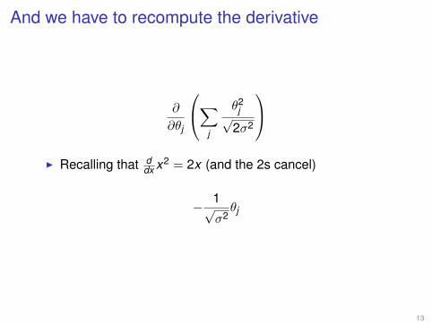
And we have to recompute the derivative
∂
∂θj
∑j
θ2j√
2σ2
I Recalling that d
dx x2 = 2x (and the 2s cancel)
− 1√σ2θj
13

What this means
I Modified log-likelihood has a penalty termI Decreased by square of each θI So large-magnitude θ get punishedI Rare features: not worth it to increase θ
I Less overfittingI More general features get smoothed less
I Prior penalty is the same, but likelihood increase is better
14

Fancier smoothing schemes
Normal distribution penalty for small weights is smallI Squared penalty
Stricter penalties:I L1: absolute value penalty
I Penalty stays significant for small weightsI Forces weights all the way to 0I Derivative doesn’t exist at µ, can use OWL-QN optimizer
(How do you pick? L2 when features are relevant but noisy, L1when most features aren’t useful at all)
15

Even fancier smoothing schemes
For instance, so-called L1, inf regularizer:
log P(D; Θ, σ) =∑
ti ,Fi∈D
log P(ti |Fi ; Θ) +λ
(maxPOS|θPOS|
)
+λ
(maxLEX|θLEX |
)+λ
(maxSUFF
|θSUFF |)
I Group features together, penalize largest weight in groupI Try to select useful groups of features
16

Should you do this?
I Always use some regularizer, even if you’re using anotherselection scheme
I Simple regularization isn’t usually enoughI Fancy regularization isn’t always available for standard
packagesI Or it may be much slower
17

External selection
Check if features on their own predict the tagI Tons and tons of methodsI Not an area I know in detail
Representative method: Chi-squaredUse Chi-squared hypothesis test to evaluate:
I Null hypothesis: fj is independent of tI If null can be rejected at some p-value, keep fjI Test doesn’t say how much information is there...
I Just that there might be some
18

Representative method: mutual informationInformation theory relates probability to encodings
I Theory of compressionI Unpredictable information takes more bits to compress
Mutual information
I(F ,T ) =∑
values f of F
∑tags t
P(F = f ,T = t) logP(F = f ,T = t)
P(F = f )P(T = t)
I If F and T independent, P(F ,T ) = P(F )P(T )I So I is 0
I Otherwise I > 0Interpretation: expected number of bits we save by encodingF ,T together rather than separately
I MI does measure strength of association19
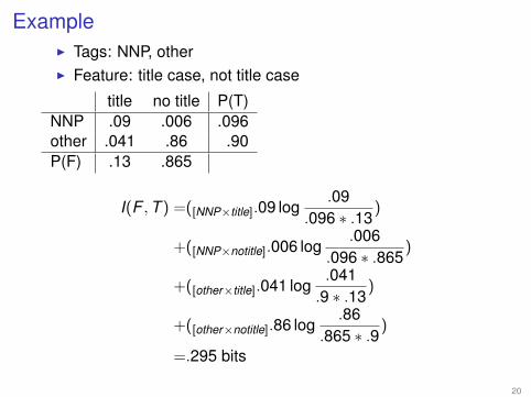
ExampleI Tags: NNP, otherI Feature: title case, not title case
title no title P(T)NNP .09 .006 .096other .041 .86 .90P(F) .13 .865
I(F ,T ) =([NNP×title].09 log.09
.096 ∗ .13)
+([NNP×notitle].006 log.006
.096 ∗ .865)
+([other×title].041 log.041.9 ∗ .13
)
+([other×notitle].86 log.86
.865 ∗ .9)
=.295 bits
20

Strengths and weaknesses
I External selection is fast...I Not distracted by relationships between featuresI Easy to interpretI Modular: Can swap classifiers easily
I External selection doesn’t care about your classifierI Beware of using a linear method and a non-linear classifier
I If features are highly correlated, you may get many copiesof information you already have
I Rare features, even important ones, often ignored
21

Step-wise selection
Stepwise forwardI Learn all possible one-feature classifiers (search over f?)I Keep the best feature f1I Learn all two-feature classifiers f1, f?I If any is better, keep the best f1, f2I ...etc
Stepwise backward (ablation)I Learn classifier using f1, f2, . . . fnI Learn all one-fewer classifiers f1, f2, fi 6=j , fnI If any one-fewer is better than original
I Throw out worst fjI Learn all two-fewer classifiers without fj , f?I ...etc
22

Comments on step-wise procedures
I Stepwise algorithms can be very slowI Lots of relearning the classifier
I However they can work better than external methodsI They control for correlationsI Once you have f1 you don’t add any copies of it
I Forward is biased toward most general featuresI Backward towards most preciseI Neither theoretically guaranteed to find the best set
I This is another optimization problemI And there is research on it!I But not mature enough to use out of the box
23

Metafeatures
Perhaps your features represent a few underlying phenomena:I “word-the”, “POS-tag-DT” are relatedI So are “preceding-word-the”, “POS-tag-NN”
I Encode underlying “definiteness” featureI This is why they are correlatedI In math terms, you have a k -dimensional feature space
I But there might only be d << k “real” dimensions
Dimensionality reductionSummarize (or “embed”) a high-dimensional space in a fewdimensions
I Or perhaps discrete clustersI A way of dealing with the curse of dimensionality
24

Principal components analysis (PCA)
Suppose we have a sample of sharks which vary along twodimensions
I Length and weightI Long sharks tend to be heavy... short sharks are usually
light
25

Really only one dimension
26
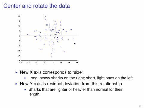
Center and rotate the data
I New X axis corresponds to “size”I Long, heavy sharks on the right; short, light ones on the left
I New Y axis is residual deviation from this relationshipI Sharks that are lighter or heavier than normal for their
length
27

Using PCA
I Make your data into a big matrixI Center and rotate itI Then throw out dimensions along which there isn’t much
varianceI “Residual” dimensions
I In this example, we’d keep new X and throw out new Y
28

Let’s see it again
image: Kendrick Kay, http://randomanalyses.blogspot.com/2012/01/principal-components-analysis.html which isworth reading in full
29

About PCA
Implemented as eigen-decompositionIssues with PCA:
I Scales badly to mega-matricesI Output matrix is dense even if input is sparse
I “Metafeatures” difficult to interpretI They incorporate information from lots of features
I Linear correlations only...I PCA doesn’t care about labels, only features
I Might destroy information your classifier will want
More advanced methods fix some of these, but at expense oftime and accessibility
30


