Feature extraction vs. feature selection Search...

CSCE 666 Pattern Analysis | Ricardo Gutierrez-Osuna | CSE@TAMU 1

L11: sequential feature selection

• Feature extraction vs. feature selection

• Search strategy and objective functions

• Objective functions – Filters

– Wrappers

• Sequential search strategies – Sequential forward selection

– Sequential backward selection

– Plus-l minus-r selection

– Bidirectional search

– Floating search


Feature extraction vs. feature selection • As discussed in L9, there are two general approaches to dim. reduction

– Feature extraction: Transform the existing features into a lower dimensional space

– Feature selection: Select a subset of the existing features without a transformation

𝑥1𝑥2

𝑥𝑁

→

𝑥𝑖1 𝑥𝑖2

𝑥𝑖𝑀

𝑥1𝑥2

𝑥𝑁

→

𝑦1𝑦2

𝑦𝑀

= 𝑓

𝑥1𝑥2

𝑥𝑁

• Feature extraction was covered in L9-10 – We derived the “optimal” linear features for two objective functions

• Signal representation: PCA

• Signal classification: LDA

• Feature selection, also called feature subset selection (FSS) in the literature, will be the subject of the last two lectures – Although FSS can be thought of as a special case of feature extraction (think of a

sparse projection matrix with a few ones), in practice it is a quite different problem

– FSS looks at the issue of dimensionality reduction from a different perspective

– FSS has a unique set of methodologies


Feature subset selection • Definition

– Given a feature set 𝑋 = {𝑥𝑖 | 𝑖 = 1…𝑁}, find a subset 𝑌𝑀, with 𝑀 < 𝑁, that maximizes an objective function 𝐽(𝑌), ideally 𝑃 𝑐𝑜𝑟𝑟𝑒𝑐𝑡

𝑌𝑀 = 𝑥𝑖1, 𝑥𝑖2, … , 𝑥𝑖𝑀 = arg ma𝑥𝑀,𝑖𝑀

𝐽 𝑥𝑖| 𝑖 = 1. . 𝑁

• Why feature subset selection? – Why not use the more general feature extraction methods, and simply

project a high-dimensional feature vector onto a low-dimensional space?

• Feature subset selection is necessary in a number of situations – Features may be expensive to obtain

• You evaluate a large number of features (sensors) in the test bed and select only a few for the final implementation

– You may want to extract meaningful rules from your classifier • When you project, the measurement units of your features (length, weight,

etc.) are lost

– Features may not be numeric, a typical situation in machine learning

• In addition, fewer features means fewer model parameters – Improved the generalization capabilities – Reduced complexity and run-time


Search strategy and objective function • FSS requires

– A search strategy to select candidate subsets

– An objective function to evaluate these candidates

• Search strategy

– Exhaustive evaluation of feature subsets involves 𝑁𝑀

combinations for a fixed value of 𝑀, and 2𝑁 combinations if 𝑀 must be optimized as well • This number of combinations is unfeasible, even for

moderate values of 𝑀 and 𝑁, so a search procedure must be used in practice

• For example, exhaustive evaluation of 10 out of 20 features involves 184,756 feature subsets; exhaustive evaluation of 10 out of 100 involves more than 1013 feature subsets [Devijver and Kittler, 1982]

– A search strategy is therefore needed to direct the FSS process as it explores the space of all possible combination of features

• Objective function – The objective function evaluates candidate subsets and

returns a measure of their “goodness”, a feedback signal used by the search strategy to select new candidates

Feature Subset Selection

Information

content Feature

subset

PR

algorithm

Objective

function

Search

Training data

Final feature subset

Complete feature set


Objective function

• Objective functions are divided in two groups – Filters: evaluate subsets by their information content, e.g., interclass

distance, statistical dependence or information-theoretic measures

– Wrappers: use a classifier to evaluate subsets by their predictive accuracy (on test data) by statistical resampling or cross-validation

F ilte r F S S

In fo rm a tio n

c o n te n t

F e a tu re

s u b s e t

M L

a lg o r ith m

O b je c t iv e

fu n c t io n

S e a rc h

T ra in in g d a ta

F in a l fe a tu re s u b s e t

C o m p le te fe a tu re s e t

W ra p p e r F S S

P re d ic t iv e

a c c u ra c y

F e a tu re

s u b s e t

P R

a lg o r ith m

P R

a lg o r ith m

S e a rc h

T ra in in g d a ta



F ilte r F S S

In fo rm a tio n

c o n te n t

F e a tu re

s u b s e t

M L

a lg o r ith m

O b je c t iv e

fu n c t io n

S e a rc h

T ra in in g d a ta



F ilte r F S S

In fo rm a tio n

c o n te n t

F e a tu re

s u b s e t

M L

a lg o r ith m

O b je c t iv e

fu n c t io n

S e a rc h

T ra in in g d a ta



W ra p p e r F S S

P re d ic t iv e

a c c u ra c y

F e a tu re

s u b s e t

P R

a lg o r ith m

P R

a lg o r ith m

S e a rc h

T ra in in g d a ta



W ra p p e r F S S

P re d ic t iv e

a c c u ra c y

F e a tu re

s u b s e t

P R

a lg o r ith m

P R

a lg o r ith m

S e a rc h

T ra in in g d a ta



F ilte r F S S

In fo rm a tio n

c o n te n t

F e a tu re

s u b s e t

M L

a lg o r ith m

O b je c t iv e

fu n c t io n

S e a rc h

T ra in in g d a ta



W ra p p e r F S S

P re d ic t iv e

a c c u ra c y

F e a tu re

s u b s e t

P R

a lg o r ith m

P R

a lg o r ith m

S e a rc h

T ra in in g d a ta



F ilte r F S S

In fo rm a tio n

c o n te n t

F e a tu re

s u b s e t

M L

a lg o r ith m

O b je c t iv e

fu n c t io n

S e a rc h

T ra in in g d a ta



F ilte r F S S

In fo rm a tio n

c o n te n t

F e a tu re

s u b s e t

M L

a lg o r ith m

O b je c t iv e

fu n c t io n

S e a rc h

T ra in in g d a ta



W ra p p e r F S S

P re d ic t iv e

a c c u ra c y

F e a tu re

s u b s e t

P R

a lg o r ith m

P R

a lg o r ith m

S e a rc h

T ra in in g d a ta



W ra p p e r F S S

P re d ic t iv e

a c c u ra c y

F e a tu re

s u b s e t

P R

a lg o r ith m

P R

a lg o r ith m

S e a rc h

T ra in in g d a ta




Filter types

• Distance or separability measures – These methods measure class separability using metrics such as

• Distance between classes: Euclidean, Mahalanobis, etc.

• Determinant of 𝑆𝑊−1𝑆𝐵 (LDA eigenvalues)

• Correlation and information-theoretic measures – These methods are based on the rationale that good feature subsets

contain features highly correlated with (predictive of) the class, yet uncorrelated with (not predictive of) each other

– Linear relation measures

• Linear relationship between variables can be measured using the correlation coefficient

𝐽 𝑌𝑀 = 𝜌𝑖𝑐 𝑀𝑖=1

𝜌𝑖𝑗 𝑀𝑗=𝑖+1

𝑀𝑖=1

• Where 𝜌𝑖𝑐 is the correlation coefficient between feature 𝑖 and the class label and 𝜌𝑖𝑗 is the correlation coefficient between features 𝑖 and 𝑗


– Non-linear relation measures

• Correlation is only capable of measuring linear dependence

• A more powerful measure is the mutual information 𝐼(𝑌𝑘; 𝐶)

𝐽 𝑌𝑀 = 𝐼 𝑌𝑀; 𝐶 = 𝐻 𝐶 − 𝐻 𝐶|𝑌𝑀 = 𝑝 𝑌𝑀, 𝜔𝑐 𝑙𝑜𝑔𝑝 𝑌𝑀, 𝜔𝑐𝑝 𝑌𝑀 𝑃 𝜔𝑐

𝑑𝑥𝑌𝑀

𝐶

𝑐=1

• The mutual information between the feature vector and the class label 𝐼(𝑌𝑀; 𝐶) measures the amount by which the uncertainty in the class 𝐻(𝐶) is decreased by knowledge of the feature vector 𝐻(𝐶|𝑌𝑀), where 𝐻(·) is the entropy function

• Note that mutual information requires the computation of the multivariate densities 𝑝(𝑌𝑀) and 𝑝 𝑌𝑀, 𝜔𝑐 , which is ill-posed for high-dimensional spaces

• In practice [Battiti, 1994], mutual information is replaced by a heuristic such as

𝐽 𝑌𝑀 = 𝐼 𝑥𝑖𝑚; 𝐶

𝑀

𝑚=1

− 𝛽 𝐼 𝑥𝑖𝑚; 𝑥𝑖𝑛

𝑀

𝑛=𝑚+1

𝑀

𝑚=1


Filters vs. wrappers • Filters

– Fast execution (+): Filters generally involve a non-iterative computation on the dataset, which can execute much faster than a classifier training session

– Generality (+): Since filters evaluate the intrinsic properties of the data, rather than their interactions with a particular classifier, their results exhibit more generality: the solution will be “good” for a larger family of classifiers

– Tendency to select large subsets (-): Since the filter objective functions are generally monotonic, the filter tends to select the full feature set as the optimal solution. This forces the user to select an arbitrary cutoff on the number of features to be selected

• Wrappers – Accuracy (+): wrappers generally achieve better recognition rates than filters since

they are tuned to the specific interactions between the classifier and the dataset

– Ability to generalize (+): wrappers have a mechanism to avoid overfitting, since they typically use cross-validation measures of predictive accuracy

– Slow execution (-): since the wrapper must train a classifier for each feature subset (or several classifiers if cross-validation is used), the method can become unfeasible for computationally intensive methods

– Lack of generality (-): the solution lacks generality since it is tied to the bias of the classifier used in the evaluation function. The “optimal” feature subset will be specific to the classifier under consideration


Search strategies • Exponential algorithms (Lecture 12)

– Evaluate a number of subsets that grows exponentially with the dimensionality of the search space • Exhaustive Search (already discussed)

• Branch and Bound

• Approximate Monotonicity with Branch and Bound

• Beam Search

• Sequential algorithms (Lecture 11) – Add or remove features sequentially, but have a tendency to become trapped in

local minima • Sequential Forward Selection

• Sequential Backward Selection

• Plus-l Minus-r Selection

• Bidirectional Search

• Sequential Floating Selection

• Randomized algorithms (Lecture 12) – Incorporate randomness into their search procedure to escape local minima

• Random Generation plus Sequential Selection

• Simulated Annealing

• Genetic Algorithms


Naïve sequential feature selection • One may be tempted to evaluate each individual

feature separately and select the best M features – Unfortunately, this strategy RARELY works since it does not

account for feature dependence

• Example – The figures show a 4D problem with 5 classes

– Any reasonable objective function will rank features according to this sequence: 𝐽(𝑥1) > 𝐽(𝑥2) ≈ 𝐽(𝑥3) > 𝐽(𝑥4) • 𝑥1 is the best feature: it separates 𝜔1, 𝜔2, 𝜔3 and 𝜔4, 𝜔5

• 𝑥2 and 𝑥3 are equivalent, and separate classes in three groups

• 𝑥4 is the worst feature: it can only separate 𝜔4 from 𝜔5

– The optimal feature subset turns out to be {𝑥1, 𝑥4}, because 𝑥4 provides the only information that 𝑥1 needs: discrimination between classes 𝜔4 and 𝜔5

– However, if we were to choose features according to the individual scores 𝐽(𝑥𝑘), we would certainly pick 𝑥1 and either 𝑥2 or 𝑥3, leaving classes 𝜔4 and 𝜔5 non separable • This naïve strategy fails because it does not consider features

with complementary information


Sequential forward selection (SFS) • SFS is the simplest greedy search algorithm

– Starting from the empty set, sequentially add the feature 𝑥+ that maximizes 𝐽(𝑌𝑘 + 𝑥

+) when combined with the features 𝑌𝑘 that have already been selected

• Notes – SFS performs best when the optimal subset is small

• When the search is near the empty set, a large number of states can be potentially evaluated

• Towards the full set, the region examined by SFS is narrower since most features have already been selected

– The search space is drawn like an ellipse to emphasize the fact that there are fewer states towards the full or empty sets • The main disadvantage of SFS is that it is unable

to remove features that become obsolete after the addition of other features

1. Start with the empty set 𝑌0 = {∅} 2. Select the next best feature 𝑥+ = arg max

𝑥∉𝑌𝑘

𝐽 𝑌𝑘 + 𝑥

3. Update 𝑌𝑘+1 = 𝑌𝑘 + 𝑥+; 𝑘 = 𝑘 + 1

4. Go to 2

Empty feature set

Full feature set

0 0 0 0

1 0 0 0 0 1 0 0 0 0 1 0 0 0 0 1

1 1 0 0 1 0 1 0 1 0 0 1 0 1 1 0 0 1 0 1 0 0 1 1

1 1 1 0 1 1 0 1 1 0 1 1 0 1 1 1

1 1 1 1


Example

• Run SFS to completion for the following objective function 𝐽 𝑋 = −2𝑥1𝑥2 + 3𝑥1 + 5𝑥2 − 2𝑥1𝑥2𝑥3 + 7𝑥3 + 4𝑥4 − 2𝑥1𝑥2𝑥3𝑥4

• where 𝑥𝑘 are indicator variables, which indicate whether the 𝑘𝑡ℎ feature has been selected 𝑥𝑘 = 1 or not 𝑥𝑘 = 0

• Solution

J(x1)=3 J(x2)=5 J(x3)=7 J(x4)=4

J(x3x1)=10 J(x3x2)=12 J(x3x4)=11

J(x3x2x1)=11 J(x3x2x4)=16

J(x3x2x4x1)=13


Sequential backward selection (SBS)

• SBS works in the opposite direction of SFS – Starting from the full set, sequentially remove the feature 𝑥− that

least reduces the value of the objective function 𝐽(𝑌 − 𝑥−)

• Removing a feature may actually increase the objective function 𝐽(𝑌𝑘 − 𝑥

−) > 𝐽(𝑌𝑘); such functions are said to be non-monotonic (more on this when we cover Branch and Bound)

• Notes – SBS works best when the optimal feature subset

is large, since SBS spends most of its time visiting large subsets

– The main limitation of SBS is its inability to reevaluate the usefulness of a feature after it has been discarded

1. Start with the full set 𝑌0 = 𝑋 2. Remove the worst feature 𝑥− = arg max

𝑥∈𝑌𝑘

𝐽 𝑌𝑘 − 𝑥

3. Update 𝑌𝑘+1 = 𝑌𝑘 − 𝑥−; 𝑘 = 𝑘 + 1

4. Go to 2

Empty feature set

Full feature set


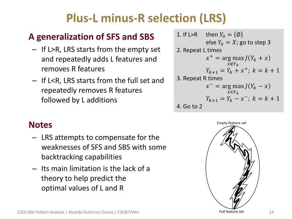
Plus-L minus-R selection (LRS)

• A generalization of SFS and SBS – If L>R, LRS starts from the empty set

and repeatedly adds L features and removes R features

– If L<R, LRS starts from the full set and repeatedly removes R features followed by L additions

• Notes – LRS attempts to compensate for the

weaknesses of SFS and SBS with some backtracking capabilities

– Its main limitation is the lack of a theory to help predict the optimal values of L and R

1. If L>R then 𝑌0 = ∅ else 𝑌0 = 𝑋; go to step 3

2. Repeat L times 𝑥+ = arg max

𝑥∉𝑌𝑘


𝑌𝑘+1 = 𝑌𝑘 + 𝑥+; 𝑘 = 𝑘 + 1

3. Repeat R times 𝑥− = arg max

𝑥∈𝑌𝑘


𝑌𝑘+1 = 𝑌𝑘 − 𝑥−; 𝑘 = 𝑘 + 1

4. Go to 2

Empty feature set

Full feature set


Bidirectional Search (BDS)

• BDS is a parallel implementation of SFS and SBS – SFS is performed from the empty set

– SBS is performed from the full set

– To guarantee that SFS and SBS converge to the same solution

• Features already selected by SFS are not removed by SBS

• Features already removed by SBS are not selected by SFS

Empty feature set

Full feature set

1. Start SFS with 𝑌𝐹 = ∅ 2. Start SBS with 𝑌𝐵 = 𝑋 3. Select the best feature

𝑥+ = arg max𝑥∉𝑌𝐹𝑘

𝑥∈F𝐵𝑘

𝐽 𝑌𝐹𝑘 + 𝑥

𝑌𝐹𝑘+1 = 𝑌𝐹𝑘 + 𝑥+

4. Remove the worst feature

𝑥− = arg max𝑥∈𝑌𝐵𝑘𝑥∉𝑌𝐹𝑘+1

𝐽 𝑌𝐵𝑘 − 𝑥

𝑌𝐵𝑘+1 = 𝑌𝐵𝑘 − 𝑥−; 𝑘 = 𝑘 + 1

5. Go to 2


Sequential floating selection (SFFS and SFBS)

• An extension to LRS with flexible backtracking capabilities – Rather than fixing the values of L and R, these floating methods allow

those values to be determined from the data:

– The dimensionality of the subset during the search can be thought to be “floating” up and down

• There are two floating methods – Sequential floating forward selection (SFFS) starts from the empty set

• After each forward step, SFFS performs backward steps as long as the objective function increases

– Sequential floating backward selection (SFBS) starts from the full set

• After each backward step, SFBS performs forward steps as long as the objective function increases


• SFFS Algorithm (SFBS is analogous)

Empty feature set

Full feature set

1. 𝑌 = ∅ 2. Select the best feature 𝑥+ = arg max

𝑥∉𝑌𝑘


𝑌𝑘 = 𝑌𝑘 + 𝑥+; 𝑘 = 𝑘 + 1

3. Select the worst feature* 𝑥− = arg max

𝑥∈𝑌𝑘


4. If 𝐽 𝑌𝑘 − 𝑥− > 𝐽 𝑌𝑘 then

𝑌𝑘+1 = 𝑌𝑘 − 𝑥−; 𝑘 = 𝑘 + 1

Go to step 3 Else Go to step 2

*Notice that you’ll need to do book-keeping to avoid infinite loops

Feature extraction vs. feature selection Search...

Documents

Transcript of Feature extraction vs. feature selection Search...