Feature Extraction from Histopathological ImagesBased on Nucleus-Guided Convolutional Neural

Network for Breast Lesion Classification

Yushan Zhenga,b, Zhiguo Jianga,b,∗∗, Fengying Xiea,b,∗, Haopeng Zhanga,b,Yibing Maa,b, Huaqiang Shic,d, Yu Zhaoc

5

aImage Processing Center, School of Astronautics, Beihang University, Beijing, 100191,China, {yszheng, jiangzg, xfy 73, zhanghaopeng, mayibing@buaa.edu.cn}

bBeijing Key Laboratory of Digital Media, Beijing, 100191, ChinacMotic (Xiamen) Medical Diagnostic Systems Co. Ltd., Xiamen, 361101, China, {shihq,

zhaoy@motic.com}10

dGeneral Hospital of the Air Force, PLA, Beijing, 100036, China

Abstract

Feature extraction is a crucial and challenging aspect in the computer-aided

diagnosis of breast cancer with histopathological images. In recent years, many

machine learning methods have been introduced to extract features from histo-

pathological images. In this study, a novel nucleus-guided feature extraction

framework based on convolutional neural network is proposed for histopatho-

logical images. The nuclei are first detected from images, and then used to

train a designed convolutional neural network with three hierarchy structures.

Through the trained network, image-level features including the pattern and

spatial distribution of the nuclei are extracted. The proposed features are

evaluated through the classification experiment on a histopathological image

database of breast lesions. The experimental results show that the extracted

features effectively represent histopathological images, and the proposed frame-

work achieves a better classification performance for breast lesions than the

compared state-of-the-art methods.

Keywords: Feature extraction, histopathological image, breast cancer,

convolutional neural network, computer-aided diagnosis

∗Corresponding author: Fengying Xie, Tel.:+86 010 82339520.∗∗Corresponding author: Zhiguo Jiang, Tel.:+86 010 82338061.

Preprint submitted to Pattern Recognition April 25, 2017

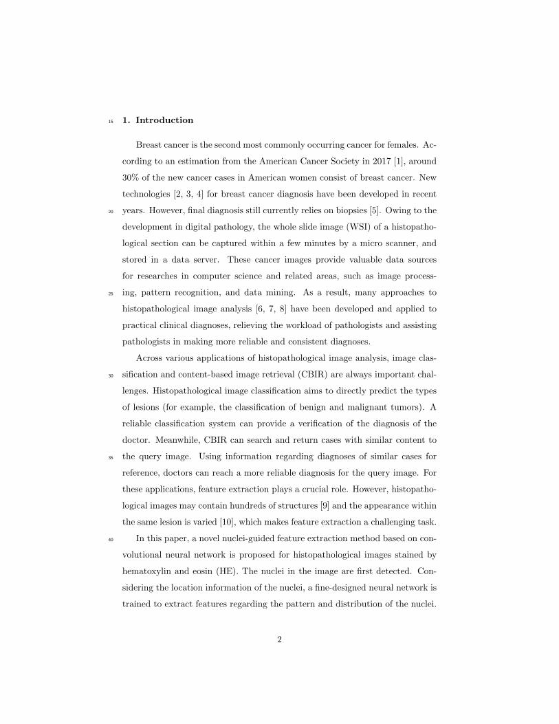
1. Introduction15

Breast cancer is the second most commonly occurring cancer for females. Ac-

cording to an estimation from the American Cancer Society in 2017 [1], around

30% of the new cancer cases in American women consist of breast cancer. New

technologies [2, 3, 4] for breast cancer diagnosis have been developed in recent

years. However, final diagnosis still currently relies on biopsies [5]. Owing to the20

development in digital pathology, the whole slide image (WSI) of a histopatho-

logical section can be captured within a few minutes by a micro scanner, and

stored in a data server. These cancer images provide valuable data sources

for researches in computer science and related areas, such as image process-

ing, pattern recognition, and data mining. As a result, many approaches to25

histopathological image analysis [6, 7, 8] have been developed and applied to

practical clinical diagnoses, relieving the workload of pathologists and assisting

pathologists in making more reliable and consistent diagnoses.

Across various applications of histopathological image analysis, image clas-

sification and content-based image retrieval (CBIR) are always important chal-30

lenges. Histopathological image classification aims to directly predict the types

of lesions (for example, the classification of benign and malignant tumors). A

reliable classification system can provide a verification of the diagnosis of the

doctor. Meanwhile, CBIR can search and return cases with similar content to

the query image. Using information regarding diagnoses of similar cases for35

reference, doctors can reach a more reliable diagnosis for the query image. For

these applications, feature extraction plays a crucial role. However, histopatho-

logical images may contain hundreds of structures [9] and the appearance within

the same lesion is varied [10], which makes feature extraction a challenging task.

In this paper, a novel nuclei-guided feature extraction method based on con-40

volutional neural network is proposed for histopathological images stained by

hematoxylin and eosin (HE). The nuclei in the image are first detected. Con-

sidering the location information of the nuclei, a fine-designed neural network is

trained to extract features regarding the pattern and distribution of the nuclei.

2

Through classification experiments on a breast-lesion database, the proposed45

features are validated to be effective for histopathological images.

The remainder of this paper is organized as follows. Section II reviews

relevant work regarding histopathological image analysis. Section III introduces

the proposed feature extraction method. The experiment and discussion are

presented in Section IV and Section V. Finally, Section VI summarises the50

present contributions and suggests directions for future work.

2. Related Work

Many feature extraction methods have been proposed for histopathological

images. They can be broadly classified into two categories: statistics based

method and learning based method.55

Inspired by the success of natural image analysis, some researchers [11, 12,

13, 14] have employed classical feature descriptors, such as color histograms,

scale-invariant feature transform (SIFT)[15], histogram of oriented gradient

(HOG)[16], and local binary pattern (LBP)[17], to depict histopathological im-

ages. Although the characteristics of cancer in histopathological images are60

quite different from those in natural images, classical features have achieved

considerable success in histopathological analysis. Simultaneously, several re-

searchers [18, 19, 20] have tended to describe images in terms of pathological

aspects. In [19], the statistics regarding the shape, size, distribution of the

nuclei are computed to give the histopathological image representation. The65

statistics can describe the general status of the nuclei, but may weaken the

response of key nuclei that are few but important for diagnosis. Further, to

describe meaningful objects in the histopathological images (such as glands and

ducts), graph-based features [21, 22] were introduced to histopathological im-

age analysis. To establish more comprehensive representations, mixed features70

[23, 24, 25, 26, 27, 28, 29] have been proposed, and achieve a better perfor-

mance. In [27], Kandemir et al. represented the histopathological images by

mixing color histogram, SIFT, LBP and a set of well-designed nuclear features,

3

and analyzed the necessities of patterns from color, texture and nuclear statis-

tics.75

With the development of machine learning, several feature learning methods,

including auto-encoders [30, 31, 32], restricted Boltzmann machines [33, 34],

sparse representation [35, 36, 37], and convolutional neural network (CNN)

[38, 39, 40], have been introduced to mine patterns from the raw pixel data of

histopathological images. In [33], sparse features were extracted from patches80

using a restricted Boltzmann machine, and then quantified into the image-level

feature through a max-pooling process. In [30], sparse auto-encoders are ap-

plied to learn a set of feature extractors for histopathological images. Then,

the feature maps are obtained through convolutional operations on the feature

extractors and the image. Furthermore, in [31], a stacked feature representa-85

tion was appended to the former framework. In [39], Xu et al. applied a deep

convolutional neural network to analyze and classify the epithelial and stromal

regions in histopathological images. In these approaches, the features are ex-

tracted patch by patch throughout the histopathological image, which ignored

the characteristics of histopathological images and resulted in a high computa-90

tional complexity. In contrast, Srinivas et al. [36] proposed a sparsity model

to encode cellular patches that selected by a blob detection approach, and then

classified histopathological images by fusing the predictions of these cellular

patches. As a continuation of this work, Vu et al. [37] proposed a class-specific

dictionary learning method for the sparsity model. Using this dictionary, more95

discriminative sparse representations of image patches were extracted. This

patch-selected scheme of [36, 37] sharply reduces the running time, but often

failed to identify the malignant samples when the malignant area is minority in

the image.

In this paper, we propose a novel nuclei-guided convolutional neural network100

to learn features from histopathological images. Unlike in a normal CNN, the

activations on the first convolutional layer are limited to the key patches, which

are selected by an efficient nucleus detection algorithm. Compared with existing

patch-based methods [41, 42, 36, 37], in which the image-level prediction is

4

obtained by fusing the predictions of key patches, we generate the patch-level105

and image-level features and the image classification criteria simultaneously

during an end-to-end learning process. Through a classification experiment on

a breast-lesion database, the proposed features are verified to be both effective

and efficient for histopathological image representation and classification.

Figure 1: Flowchart of the training stage.

3. Method110

According to pathologists [5, 43], the appearance of the cell nucleus and

its surrounding cytoplasm, as well as the distribution of nuclei, are important

indicators for cancer diagnosis. Therefore, both the appearance and distribution

of nuclei are considered. The proposed framework consists of an offline training

stage and an online encoding stage, where the former can be divided into three115

steps: nuclei detection, pre-training, and fine-tuning.

Figure 1 presents a flowchart of the training stage. the cell nuclei are first

detected. Then, a fine-designed neural network is constructed under the guide of

nucleus locations to extract image-level features. The neural network consists of

5

Figure 2: An instance of nuclei detection. Here, (a) is the original image, (b) is the hematoxylin

component separated by color deconvolution, (c) is the result obtained by Gaussian filtering,

(d) shows the positions of local maxima, and (e) is the detection result, in which some instances

of nucleus patches are displayed in red boxes.

three basic structures from the bottom to the top: the patch-level, block-level,120

and image-level structure. The patch-level structure contains a convolutional

layer and a non-linear layer. Both the block-level and image-level structures

consist of a pooling layer, a full-connecting layer, and a non-linear layer.

Plenty of labeled histopathological images are required to train an effective

deep neural network if the biases and weights of the network are randomly125

initialized. However, it is a difficult task to produce a complete annotation for

a whole slide image (WSI), even for an experienced pathologist. Therefore, we

proposed to first pre-train the network with abundant unlabeled regions, and

then fine-tune it using the labeled images.

3.1. Nucleus detection130

In this paper, the nuclei are located using a blob detection method. To

remove noises caused by stroma, the nucleus component H (i.e., the optical

density of the hematoxylin component in the HE-stained histopathological im-

age) is first extracted using the color deconvolution algorithm [44]. Then, a

Gaussian filter is employed to highlight the cell nuclei in H, thus providing a135

6

probability map of cell nuclei:

Hnuc = H ∗G(ξ), (1)

where ∗ denotes the convolution operation, G(ξ) is a Gaussian with mean 0

and scale ξ. In this paper, ξ is determined experimentally as 6.5, and the size

of the Gaussian filter is 13×13, which can cover most of the nuclei under a 20×

lens.140

By searching for local maxima in Hnuc, the nuclei are coarsely detected. At

the same time, some noise will also be detected. Considering that these noises

have weak responses in Hnuc, a threshold is used to filter them out. Figure 2

illustrates an instance of nuclei detection, where (a) is the original image and (e)

shows the detection result. It can be seen that the nuclei are located effectively.145

In next section, patches centered on nuclei are sampled (see the red box in

Figure 2(e)), and used to mine the histopathological features.

3.2. Pre-training

Auto-encoder(AE) can remove redundancies and noises, and mine the dis-

criminative pattern for unlabeled data, which has proven effective in pre-training150

network parameters [45, 46]. However, for histopathological images, the dif-

ference among nuclei appearance is much more important for the diagnosis of

breast lesions than the difference between nuclei and stroma. If AE is conducted

on entire image, the discrimination among nuclei appearance in the extracted

features will be weakened. Therefore, in our method, only nucleus locations are155

considered in the training of AE.

3.2.1. Patch-level structure

A convolutional layer is first employed to extract basic features from the raw

pixel data. In this paper, only nuclei are considered for constructing the feature

extraction network, thus the computation for stromal regions are unnecessary.

As shown in Figure 2(e), the nuclei are spatially sparse and scarcely overlap

with each other. Therefore, we propose to take nuclei as independent samples

7

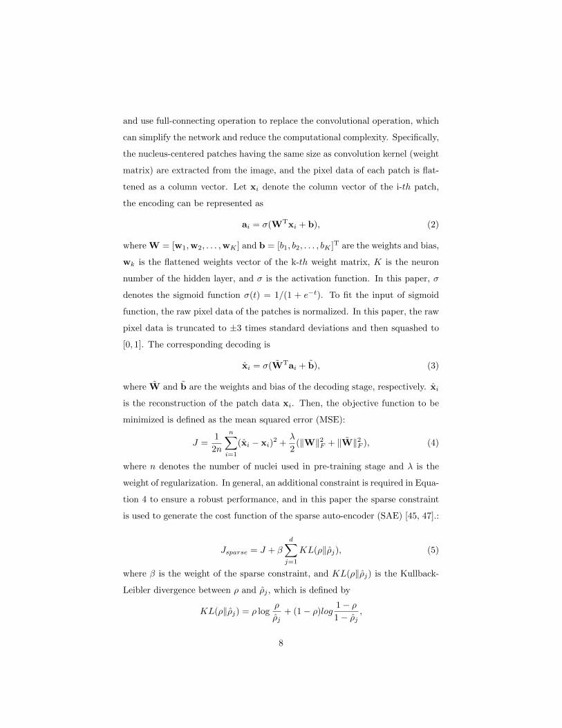
and use full-connecting operation to replace the convolutional operation, which

can simplify the network and reduce the computational complexity. Specifically,

the nucleus-centered patches having the same size as convolution kernel (weight

matrix) are extracted from the image, and the pixel data of each patch is flat-

tened as a column vector. Let xi denote the column vector of the i-th patch,

the encoding can be represented as

ai = σ(WTxi + b), (2)

where W = [w1,w2, . . . ,wK ] and b = [b1, b2, . . . , bK ]T are the weights and bias,

wk is the flattened weights vector of the k-th weight matrix, K is the neuron

number of the hidden layer, and σ is the activation function. In this paper, σ

denotes the sigmoid function σ(t) = 1/(1 + e−t). To fit the input of sigmoid

function, the raw pixel data of the patches is normalized. In this paper, the raw

pixel data is truncated to ±3 times standard deviations and then squashed to

[0, 1]. The corresponding decoding is

xi = σ(WTai + b), (3)

where W and b are the weights and bias of the decoding stage, respectively. xi

is the reconstruction of the patch data xi. Then, the objective function to be

minimized is defined as the mean squared error (MSE):

J =1

2n

n∑i=1

(xi − xi)2 +

λ

2(‖W‖2F + ‖W‖2F ), (4)

where n denotes the number of nuclei used in pre-training stage and λ is the

weight of regularization. In general, an additional constraint is required in Equa-

tion 4 to ensure a robust performance, and in this paper the sparse constraint

is used to generate the cost function of the sparse auto-encoder (SAE) [45, 47].:

Jsparse = J + β

d∑j=1

KL(ρ‖ρj), (5)

where β is the weight of the sparse constraint, and KL(ρ‖ρj) is the Kullback-

Leibler divergence between ρ and ρj , which is defined by

KL(ρ‖ρj) = ρ logρ

ρj+ (1− ρ)log

1− ρ1− ρj

,

8

where ρj denotes the average value of the activations on the j-th hidden unit

over all the training patches, ρj = 1/n∑ni=1 aij and ρ is a constant that defines

the prospective average activation. For the sparse auto-encoder, ρ constrains160

the degree of the sparsity of the hidden representations. The smaller ρ is, the

more the semantics will be mined [47].

Finally, the optimal parameters can be obtained by solving the equation

(W∗,b∗,W∗, b∗) = arg minW,b,W,b

Jsparse. (6)

Through Equation 6, the hidden representations of nuclei patches (aj) are op-

timized and used for the encoding of block-level structure.

3.2.2. Block-level structure165

The image-level features can be quantified by simply pooling all of the acti-

vations of nucleus patches within the image. However, this strategy disregards

the spatial distribution of nuclei. To preserve the distribution information, the

block-level structure is inserted between the nucleus-level and image-level struc-

tures. As shown in Figure 3, the image is divided into square blocks of m×m170

pixels, in which the nucleus activations are quantified.

Let A = (a1,a2, ...,aN ) be the set of nucleus activations that are located in

the i-th block. Then, the quantified representation is defined as the max-pooling

result of A :

p(1)i = (p

(1)i1 , p

(1)i2 , ..., p

(1)iK )T = (‖A1‖∞, ‖A2‖∞, ..., ‖AK‖∞)T, (7)

where Ak denotes the k-th row of A, and ‖·‖∞ is the infinite norm. To simplify

the expression, the max-pooling operation is represented as p(1)i = maxpool(A).

Let n(1) be the number of blocks for training. Then, the representations of

the first pooling layer are defined as P(1) = (p(1)1 ,p

(1)2 , . . . ,p

(1)

n(1)). Regarding

P(1) as the input, another SAE can be trained. The activations of the second

sparse AE are defined as

A(2) = (a(2)1 ,a

(2)2 , . . . ,a

(2)

n(1)),

9

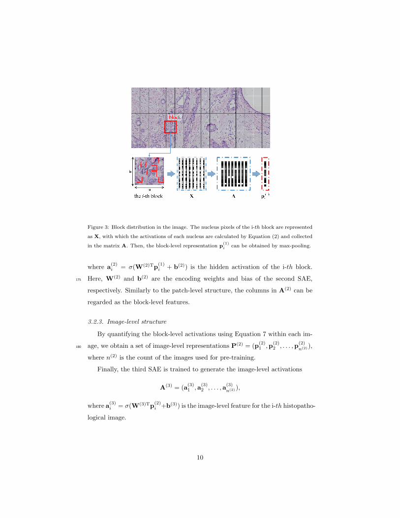
Figure 3: Block distribution in the image. The nucleus pixels of the i-th block are represented

as X, with which the activations of each nucleus are calculated by Equation (2) and collected

in the matrix A. Then, the block-level representation p(1)i can be obtained by max-pooling.

where a(2)i = σ(W(2)Tp

(1)i + b(2)) is the hidden activation of the i-th block.

Here, W(2) and b(2) are the encoding weights and bias of the second SAE,175

respectively. Similarly to the patch-level structure, the columns in A(2) can be

regarded as the block-level features.

3.2.3. Image-level structure

By quantifying the block-level activations using Equation 7 within each im-

age, we obtain a set of image-level representations P(2) = (p(2)1 ,p

(2)2 , . . . ,p

(2)

n(2)),180

where n(2) is the count of the images used for pre-training.

Finally, the third SAE is trained to generate the image-level activations

A(3) = (a(3)1 ,a

(3)2 , . . . ,a

(3)

n(2)),

where a(3)i = σ(W(3)Tp

(2)i +b(3)) is the image-level feature for the i-th histopatho-

logical image.

10

3.3. Fine-tuning

Following pre-training, the three basic structures are stacked to construct185

the integrated network, which can extract image-level features of the histopatho-

logical image. Since the weights and biases in the three structures are trained

separately in greedy manner, they are not globally optimal for the stacked neu-

ral network. Therefore, a softmax layer is connected to the final hidden layer

of the network, utilizing the supervised information to further optimize the190

network parameters. Then, the whole network is fine-tuned with the labeled

histopathological images using the L-BFGS [48] algorithm. For the end-to-end

supervised learning stage, more discriminative patterns for the descriptions of

the histopathological images can be mined.

3.4. Encoding195

Given a histopathological image, the nuclei are first detected, and then the

patches of the nuclei are fed into the fine-tuned network to obtain the image-level

features. Algorithm 1 presents the pseudo-code of the encoding. The proposed

features are output from the last hidden layer (before the softmax layer). By

putting these features into a classifier, the image can be classified.200

4. Experiment

In this paper, a novel nucleus-guided feature extraction framework based

on CNN is proposed for histopathological images. The proposed algorithm is

implemented in Matlab 2013a on the PC with a 12 Intel Core Processor (2.10

GHz) and a GPU of Nvidia Tesla k40. The implementation of the whole network205

is based on the UFLDL tutorial1.

The performance of the proposed method is evaluated using a fine-annotated

histopathological image database of breast lesions. Experiments are conducted

1https://github.com/amaas/stanford dl ex [accessed 2017.04.19]

11

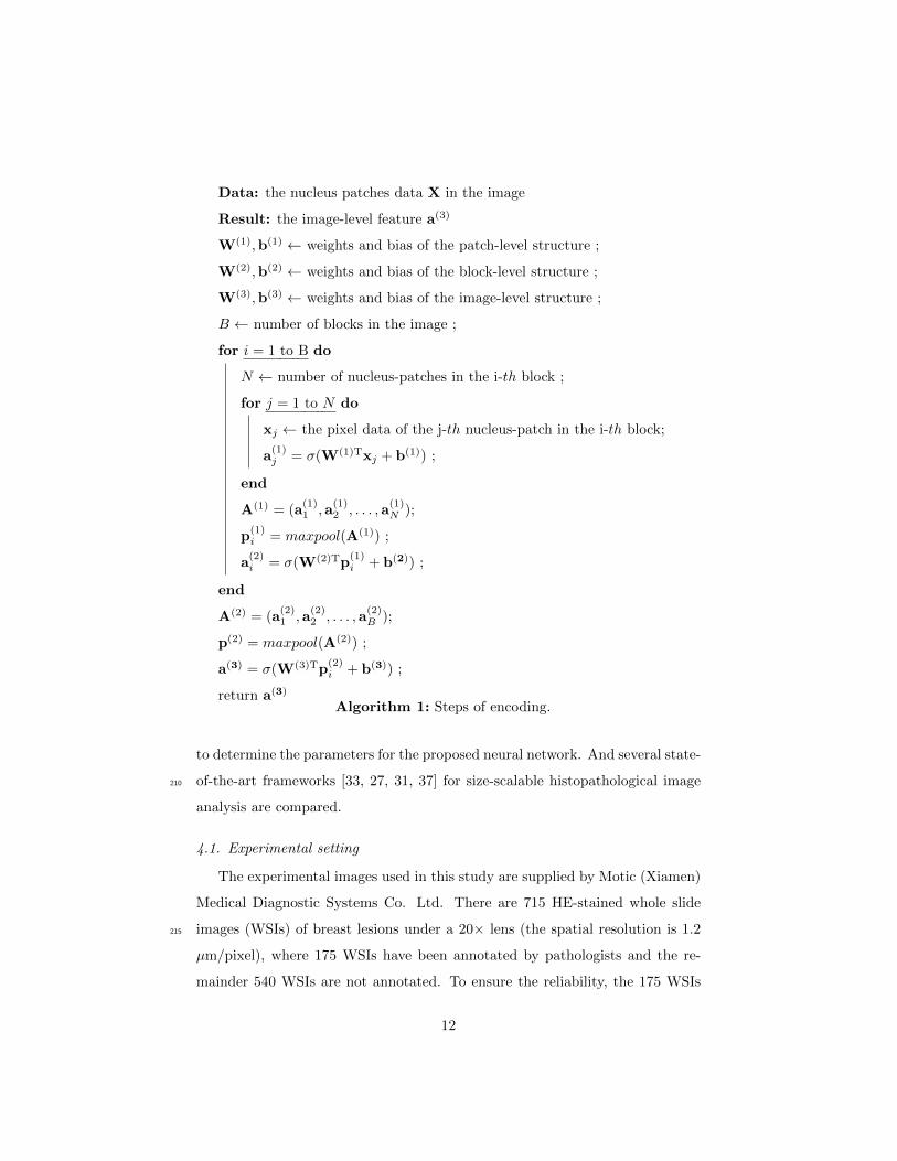
Data: the nucleus patches data X in the image

Result: the image-level feature a(3)

W(1),b(1) ← weights and bias of the patch-level structure ;

W(2),b(2) ← weights and bias of the block-level structure ;

W(3),b(3) ← weights and bias of the image-level structure ;

B ← number of blocks in the image ;

for i = 1 to B do

N ← number of nucleus-patches in the i-th block ;

for j = 1 to N do

xj ← the pixel data of the j-th nucleus-patch in the i-th block;

a(1)j = σ(W(1)Txj + b(1)) ;

end

A(1) = (a(1)1 ,a

(1)2 , . . . ,a

(1)N );

p(1)i = maxpool(A(1)) ;

a(2)i = σ(W(2)Tp

(1)i + b(2)) ;

end

A(2) = (a(2)1 ,a

(2)2 , . . . ,a

(2)B );

p(2) = maxpool(A(2)) ;

a(3) = σ(W(3)Tp(2)i + b(3)) ;

return a(3)

Algorithm 1: Steps of encoding.

to determine the parameters for the proposed neural network. And several state-

of-the-art frameworks [33, 27, 31, 37] for size-scalable histopathological image210

analysis are compared.

4.1. Experimental setting

The experimental images used in this study are supplied by Motic (Xiamen)

Medical Diagnostic Systems Co. Ltd. There are 715 HE-stained whole slide

images (WSIs) of breast lesions under a 20× lens (the spatial resolution is 1.2215

µm/pixel), where 175 WSIs have been annotated by pathologists and the re-

mainder 540 WSIs are not annotated. To ensure the reliability, the 175 WSIs

12

have been independently annotated by two pathologists, and the final annota-

tions are judged by a third pathologist. Using the 175 WSIs, two datasets of

labeled images are established:220

• The 2-class dataset: 2013 and 2096 labeled images with 256K-1536K pixels

are respectively sampled from the annotated regions of malignant and

benign breast tumors, generating a 2-class dataset.

• The 15-class dataset: Images in the 2-class dataset are fine-classified into

13 sub-categories of breast tumors according to the world health organi-225

zation (WHO) standard [10]. In addition, images of the non-neoplastic

lesions and healthy tissue are sampled as two further categories. Conse-

quently, a 15-class dataset containing 4470 labeled images is established.

The details of the 15-class dataset are listed in Table 1, and a representa-

tive image of each category is presented in Figure 4.230

For both the 2-class and 15-class datasets, a quarter of samples are used for

testing, and the remainder for training.

For the 2-class dataset, three metrics including sensitivity, specificity, accu-

racy of classification are used to evaluate the algorithm performance, which are

defined by equations:

Sensitivity =TP

P, Specificity =

TN

N,Accuracy =

TP + TN

P +N. (8)

where TP denotes the number of correctly identified malignant samples, TN

denotes the number of correctly identified benign samples, P and N are the

number of malignant and benign samples, respectively. Similarly, for the 15-235

class dataset, the sensitivity and total classification accuracy are used. Let Si

denote the number of samples belonging to the i-th class lesion and Ti be the

number of correctly identified samples in the i-th class lesion, the sensitivity for

the i-th class lesion is defined as Ti/Si and the total accuracy is calculated by

equation∑15i=1 Ti/

∑15i=1 Si.240

13

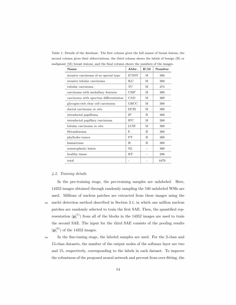
Table 1: Details of the database. The first column gives the full names of breast lesions, the

second column gives their abbreviations, the third column shows the labels of benign (B) or

malignant (M) breast lesions, and the final column shows the numbers of the images.

Name Abbr. B\M Number

invasive carcinoma of no special type ICNST M 300

invasive lobular carcinoma ILC M 300

tubular carcinoma TC M 274

carcinoma with medullary features CMF M 300

carcinoma with apocrine differentiation CAD M 300

glycogen-rich clear cell carcinoma GRCC M 300

ductal carcinoma in situ DCIS M 300

intraductal papilloma IP B 300

intraductal papillary carcinoma IPC M 300

lobular carcinoma in situ LCIS M 300

fibroadenoma F. B 300

phyllodes tumor PT B 300

hamartoma H. B 300

nonneoplastic lesion NL - 300

healthy tissue HT - 296

total - - 4470

4.2. Training details

In the pre-training stage, the pre-training samples are unlabeled. Here,

14352 images obtained through randomly sampling the 540 unlabeled WSIs are

used. Millions of nucleus patches are extracted from these images using the

nuclei detection method described in Section 3.1, in which one million nucleus245

patches are randomly selected to train the first SAE. Then, the quantified rep-

resentation (p(1)i ) from all of the blocks in the 14352 images are used to train

the second SAE. The input for the third SAE consists of the pooling results

(p(2)i ) of the 14352 images.

In the fine-tuning stage, the labeled samples are used. For the 2-class and250

15-class datasets, the number of the output nodes of the softmax layer are two

and 15, respectively, corresponding to the labels in each dataset. To improve

the robustness of the proposed neural network and prevent from over-fitting, the

14

Figure 4: Images in the database, where the malignant and benign tumors are framed by red

and blue rectangles, respectively, non-neoplastic lesions are yellow, and healthy tissue is green.

The names of the categories are (a) invasive carcinoma of no special type, (b) invasive lobular

carcinoma, (c) tubular carcinoma, (d) carcinoma with medullary features, (e) carcinoma with

apocrine differentiation, (f) glycogen-rich clear cell carcinoma, (g) ductal carcinoma in situ,

(h) intraductal papilloma, (i) intraductal papillary carcinoma, (j) lobular carcinoma in situ,

(k) fibroadenoma, (l) phyllodes tumor, (m) hamartoma, (n) nonneoplastic lesion, and (o)

healthy tissue.

images are rotated and flipped to produce data augmentation in the fine-tuning

stage.255

4.3. Parameter setting

The size of the nucleus patch is set to 11 × 11, which can cover a nucleus

and contain appropriate amount of stroma surrounding the nucleus. And three

channels in RGB color space are used. Hence, the dimension of the nucleus data

xi is 11×11×3 = 363. Seven parameters including K(1),K(2), K(3), ρ,m, λ, and260

β need to be determined, where K(1),K(2) and K(3) are the number of hidden

nodes in the three auto-encoders, ρ is the prospective sparsity mentioned in

Section 3.2.1, m is the size of block mentioned in Section 3.2.2, and λ and

β are the weights for the regularization term (Eq. 4) and the sparsity term

(Eq. 5), respectively. When determining one of the seven parameters, the other265

parameters are set as constant.

15

0 100 200 300 400 500 6000.5

0.6

0.7

0.8

0.9

1

Reconst

ructi

on e

rror

K(1)

0 100 200 300 400 5000.8

1

1.2

1.4

1.6

1.8

2

Reconst

ructi

on e

rror

K(2)

0 100 200 300 400 5000.2

0.3

0.4

0.5

0.6

0.7

Reconst

ructi

on e

rror

K(3)

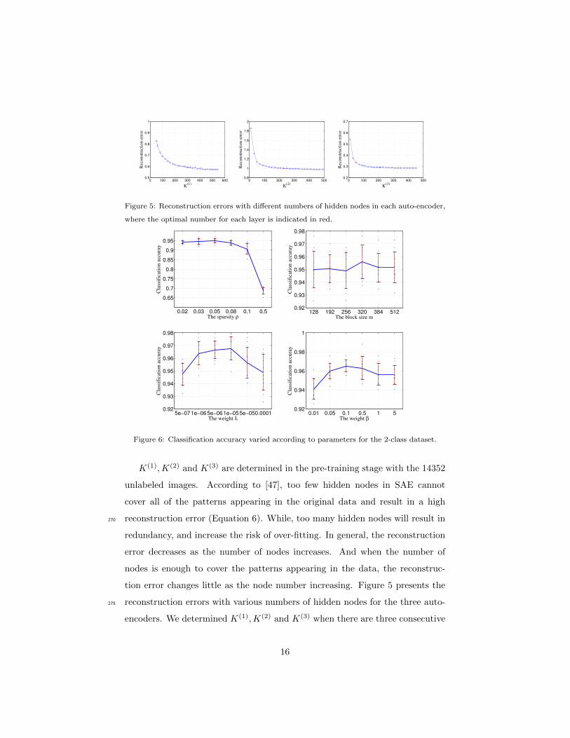
Figure 5: Reconstruction errors with different numbers of hidden nodes in each auto-encoder,

where the optimal number for each layer is indicated in red.

0.02 0.03 0.05 0.08 0.1 0.5

0.65

0.7

0.75

0.8

0.85

0.9

0.95

Cla

ssif

icat

ion

acc

ura

y

The sparsity ρ128 192 256 320 384 512

0.92

0.93

0.94

0.95

0.96

0.97

0.98

Cla

ssif

icat

ion

acc

ura

y

The block size m

5e−071e−065e−061e−055e−050.00010.92

0.93

0.94

0.95

0.96

0.97

0.98

Cla

ssif

icat

ion

acc

ura

y

The weight λ0.01 0.05 0.1 0.5 1 5

0.92

0.94

0.96

0.98

1

Cla

ssif

icat

ion

acc

ura

y

The weight β

Figure 6: Classification accuracy varied according to parameters for the 2-class dataset.

K(1),K(2) and K(3) are determined in the pre-training stage with the 14352

unlabeled images. According to [47], too few hidden nodes in SAE cannot

cover all of the patterns appearing in the original data and result in a high

reconstruction error (Equation 6). While, too many hidden nodes will result in270

redundancy, and increase the risk of over-fitting. In general, the reconstruction

error decreases as the number of nodes increases. And when the number of

nodes is enough to cover the patterns appearing in the data, the reconstruc-

tion error changes little as the node number increasing. Figure 5 presents the

reconstruction errors with various numbers of hidden nodes for the three auto-275

encoders. We determined K(1),K(2) and K(3) when there are three consecutive

16

Patch-level Block-level Image-levelPredict-

level

Conv. MP FC

MP FC FC

300 300 230

A(1) A(2) A(3)P(2)P(1)

Nuclei features

Block features

300

@11×11

Pooling

dense

dense

Notes

Conv.: convolution

FC : full-connecting

MP : max-pooling

Pooling

Block size for

2-classt: 320×320

15-class: 256×256

Image featuresLesions

prediction

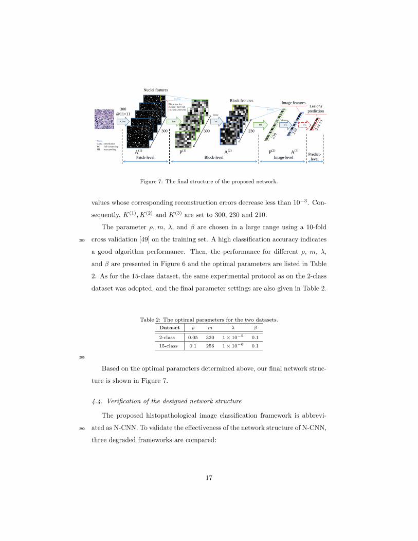
Figure 7: The final structure of the proposed network.

values whose corresponding reconstruction errors decrease less than 10−3. Con-

sequently, K(1),K(2) and K(3) are set to 300, 230 and 210.

The parameter ρ, m, λ, and β are chosen in a large range using a 10-fold

cross validation [49] on the training set. A high classification accuracy indicates280

a good algorithm performance. Then, the performance for different ρ, m, λ,

and β are presented in Figure 6 and the optimal parameters are listed in Table

2. As for the 15-class dataset, the same experimental protocol as on the 2-class

dataset was adopted, and the final parameter settings are also given in Table 2.

Table 2: The optimal parameters for the two datasets.

Dataset ρ m λ β

2-class 0.05 320 1× 10−5 0.1

15-class 0.1 256 1× 10−6 0.1

285

Based on the optimal parameters determined above, our final network struc-

ture is shown in Figure 7.

4.4. Verification of the designed network structure

The proposed histopathological image classification framework is abbrevi-

ated as N-CNN. To validate the effectiveness of the network structure of N-CNN,290

three degraded frameworks are compared:

17

• rand-CNN: The network structure is the same as N-CNN, but the patches

used on the first layer are randomly selected.

• N-CNN−: The block-level structure is omitted, and the nucleus activations

are used to directly generate the input of the image-level structure.295

• N-CNN0: The pre-trained network of N-CNN. That is, the supervised

information only impacts the softmax layer, and other hidden layers are

not fine-tuned.

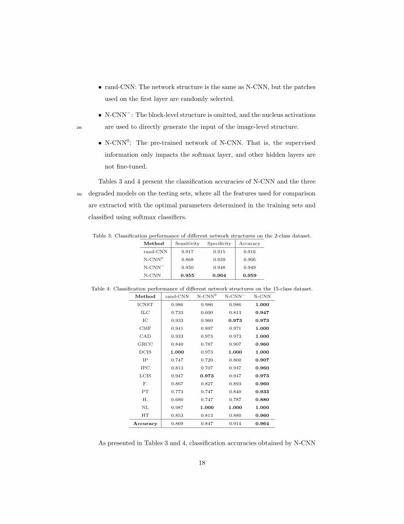
Tables 3 and 4 present the classification accuracies of N-CNN and the three

degraded models on the testing sets, where all the features used for comparison300

are extracted with the optimal parameters determined in the training sets and

classified using softmax classifiers.

Table 3: Classification performance of different network structures on the 2-class dataset.

Method Sensitivity Specificity Accuracy

rand-CNN 0.917 0.915 0.916

N-CNN0 0.868 0.939 0.906

N-CNN− 0.950 0.948 0.949

N-CNN 0.955 0.964 0.959

Table 4: Classification performance of different network structures on the 15-class dataset.

Method rand-CNN N-CNN0 N-CNN− N-CNN

ICNST 0.986 0.986 0.986 1.000

ILC 0.733 0.600 0.813 0.947

IC 0.933 0.960 0.973 0.973

CMF 0.941 0.897 0.971 1.000

CAD 0.933 0.973 0.973 1.000

GRCC 0.840 0.787 0.907 0.960

DCIS 1.000 0.973 1.000 1.000

IP 0.747 0.720 0.800 0.907

IPC 0.813 0.707 0.947 0.960

LCIS 0.947 0.973 0.947 0.973

F. 0.867 0.827 0.893 0.960

PT 0.773 0.747 0.840 0.933

H. 0.680 0.747 0.787 0.880

NL 0.987 1.000 1.000 1.000

HT 0.853 0.813 0.880 0.960

Accuracy 0.869 0.847 0.914 0.964

As presented in Tables 3 and 4, classification accuracies obtained by N-CNN

18

are much higher than those by rand-CNN. Especially for 15-class dataset, the

difference between them is 9.5%. Rand-CNN extracted features using random-305

sampled patches, which did not consider nucleus patterns. Relatively, N-CNN

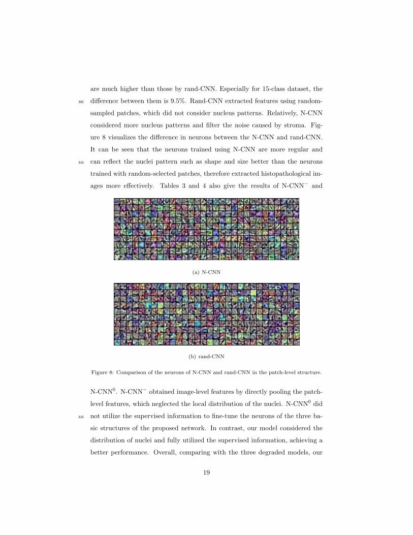
considered more nucleus patterns and filter the noise caused by stroma. Fig-

ure 8 visualizes the difference in neurons between the N-CNN and rand-CNN.

It can be seen that the neurons trained using N-CNN are more regular and

can reflect the nuclei pattern such as shape and size better than the neurons310

trained with random-selected patches, therefore extracted histopathological im-

ages more effectively. Tables 3 and 4 also give the results of N-CNN− and

(a) N-CNN

(b) rand-CNN

Figure 8: Comparison of the neurons of N-CNN and rand-CNN in the patch-level structure.

N-CNN0. N-CNN− obtained image-level features by directly pooling the patch-

level features, which neglected the local distribution of the nuclei. N-CNN0 did

not utilize the supervised information to fine-tune the neurons of the three ba-315

sic structures of the proposed network. In contrast, our model considered the

distribution of nuclei and fully utilized the supervised information, achieving a

better performance. Overall, comparing with the three degraded models, our

19

Table 5: Classification Accuracy for various number of layers between image-level representa-

tion and the softmax layer.

#Layer 1 2 3 4

2-class 0.959 0.955 0.957 0.544

15-class 0.964 0.965 0.955 0.843

designed model has the best classification accuracy, which means the structure

of our designed model is better than the three degraded models.320

Furthermore, more layers containing full-connecting and non-linear units can

be employed between the image-level representation and the softmax layer. In

this paper, a single layer is adopted. The classification accuracy using different

number of layers between the image-level representation layer and softmax layer

are presented in Table 5. It can be seen that, the classification precision changes325

little when layers increase from one to three and dramatically decreases when

the fourth layer is inserted. Therefore, a single layer is appropriate for the

proposed network.

4.5. The robustness of the proposed feature

The classifier used in N-CNN is a softmax classifier. To evaluate the ro-330

bustness of the proposed feature, another two general classifiers were validated,

generating two further classification frameworks:

• N-CNN-SVM: The activations of the penultimate layer of N-CNN (the

image-level features A(3) mentioned in Section 3.2.3) are used as the input

of a linear SVM.335

• N-CNN-KNN: The activations of the penultimate layer of N-CNN are used

to generate a KNN classifier.

Tables 6 and 7 show the classification performance using different classifiers

on the two experimental datasets. It can be seen that N-CNN-kNN and N-

CNN-SVM achieve comparable performances with N-CNN, and all of the three340

have high classification accuracies. It indicates that the image-level features

extracted by the proposed network are robust and appropriate for describing

20

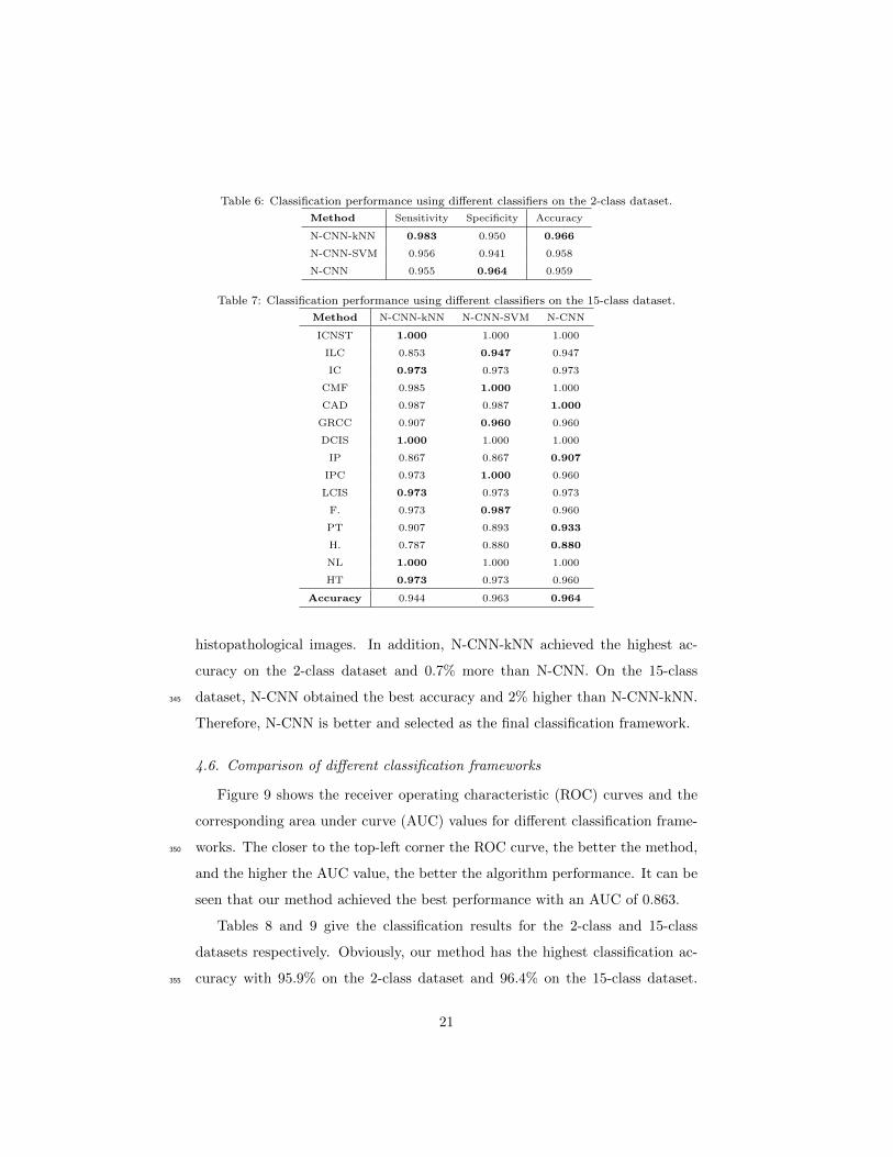
Table 6: Classification performance using different classifiers on the 2-class dataset.

Method Sensitivity Specificity Accuracy

N-CNN-kNN 0.983 0.950 0.966

N-CNN-SVM 0.956 0.941 0.958

N-CNN 0.955 0.964 0.959

Table 7: Classification performance using different classifiers on the 15-class dataset.

Method N-CNN-kNN N-CNN-SVM N-CNN

ICNST 1.000 1.000 1.000

ILC 0.853 0.947 0.947

IC 0.973 0.973 0.973

CMF 0.985 1.000 1.000

CAD 0.987 0.987 1.000

GRCC 0.907 0.960 0.960

DCIS 1.000 1.000 1.000

IP 0.867 0.867 0.907

IPC 0.973 1.000 0.960

LCIS 0.973 0.973 0.973

F. 0.973 0.987 0.960

PT 0.907 0.893 0.933

H. 0.787 0.880 0.880

NL 1.000 1.000 1.000

HT 0.973 0.973 0.960

Accuracy 0.944 0.963 0.964

histopathological images. In addition, N-CNN-kNN achieved the highest ac-

curacy on the 2-class dataset and 0.7% more than N-CNN. On the 15-class

dataset, N-CNN obtained the best accuracy and 2% higher than N-CNN-kNN.345

Therefore, N-CNN is better and selected as the final classification framework.

4.6. Comparison of different classification frameworks

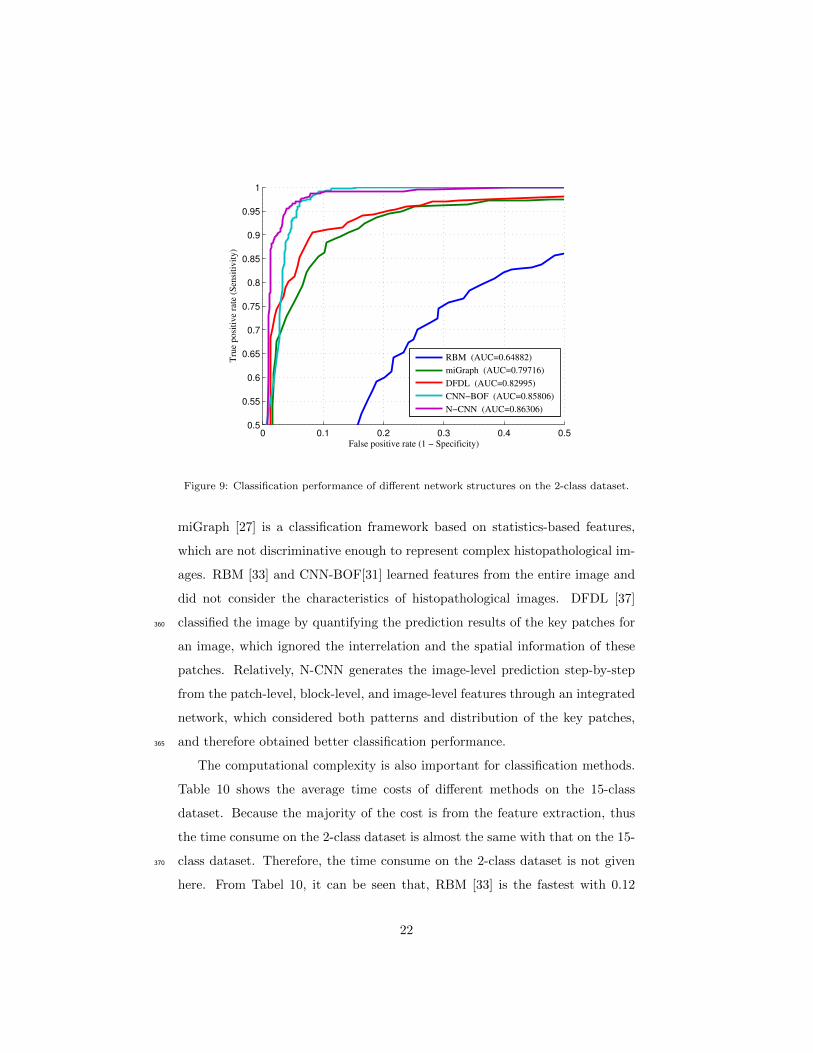
Figure 9 shows the receiver operating characteristic (ROC) curves and the

corresponding area under curve (AUC) values for different classification frame-

works. The closer to the top-left corner the ROC curve, the better the method,350

and the higher the AUC value, the better the algorithm performance. It can be

seen that our method achieved the best performance with an AUC of 0.863.

Tables 8 and 9 give the classification results for the 2-class and 15-class

datasets respectively. Obviously, our method has the highest classification ac-

curacy with 95.9% on the 2-class dataset and 96.4% on the 15-class dataset.355

21

0 0.1 0.2 0.3 0.4 0.50.5

0.55

0.6

0.65

0.7

0.75

0.8

0.85

0.9

0.95

1

False positive rate (1 − Specificity)

Tru

e p

osi

tiv

e ra

te (

Sen

siti

vit

y)

RBM (AUC=0.64882)

miGraph (AUC=0.79716)

DFDL (AUC=0.82995)

CNN−BOF (AUC=0.85806)

N−CNN (AUC=0.86306)

Figure 9: Classification performance of different network structures on the 2-class dataset.

miGraph [27] is a classification framework based on statistics-based features,

which are not discriminative enough to represent complex histopathological im-

ages. RBM [33] and CNN-BOF[31] learned features from the entire image and

did not consider the characteristics of histopathological images. DFDL [37]

classified the image by quantifying the prediction results of the key patches for360

an image, which ignored the interrelation and the spatial information of these

patches. Relatively, N-CNN generates the image-level prediction step-by-step

from the patch-level, block-level, and image-level features through an integrated

network, which considered both patterns and distribution of the key patches,

and therefore obtained better classification performance.365

The computational complexity is also important for classification methods.

Table 10 shows the average time costs of different methods on the 15-class

dataset. Because the majority of the cost is from the feature extraction, thus

the time consume on the 2-class dataset is almost the same with that on the 15-

class dataset. Therefore, the time consume on the 2-class dataset is not given370

here. From Tabel 10, it can be seen that, RBM [33] is the fastest with 0.12

22

Table 8: Classification performance of different frameworks on the 2-class dataset.

Method Sensitivity Specificity Accuracy

RBM [33] 0.746 0.708 0.726

miGraph [27] 0.862 0.893 0.879

DFDL [37] 0.904 0.917 0.911

CNN-BOF [31] 0.973 0.935 0.953

N-CNN 0.955 0.964 0.959

Table 9: Classification performance of different frameworks on the 15-class dataset.

Method RBM [33] miGraph [27] DFDL [37] CNN-BOF [31] N-CNN

ICNST 0.878 0.986 0.986 1.000 1.000

ILC 0.480 0.733 0.760 0.720 0.947

IC 0.853 0.933 0.960 0.947 0.973

CMF 0.721 0.941 0.941 0.926 1.000

CAD 0.880 0.933 0.973 0.973 1.000

GRCC 0.693 0.840 0.960 0.893 0.960

DCIS 1.000 1.000 1.000 0.987 1.000

IP 0.573 0.747 0.907 0.880 0.907

IPC 0.520 0.813 0.840 0.947 0.960

LCIS 0.880 0.947 0.960 0.960 0.973

F. 0.693 0.867 0.933 0.987 0.960

PT 0.440 0.773 0.787 0.920 0.933

H. 0.520 0.680 0.800 0.867 0.880

NL 0.840 0.987 0.987 1.000 1.000

HT 0.733 0.853 0.800 0.960 0.960

Accuracy 0.714 0.869 0.906 0.931 0.964

Table 10: Computational time for different classification frameworks (s).

RBM [33] miGraph [27] DFDL [37] CNN-BOF [31] N-CNN

0.12 11.04 1.1 7.82 0.41

second among the five compared methods, but it has the lowest classification

accuracy (see Tables 8 and 9). CNN-BOF [31] encodes all of the feasible patches

within the image, which requires a computational time of 7.82 s. Compared with

CNN-BOF, N-CNN takes a short time to search the key patches from all the375

feasible patches to encode, thus sharply reduces the computation.

Therefore, with the best classification accuracy and the second short time

cost, our proposed method greatly outperforms other compared methods.

23

5. Discussion

In this paper, the nucleus features including the pattern and spatial dis-380

tribution are extracted from histopathological images using a designed CNN

combined with the guide of nuclei, which has good classification performance

for breast lesions. Regarding the proposed method, we have the following dis-

cussion:

5.1. Differences between normal CNNs and the proposed network385

The first layer of the proposed network is a convolutional layer. In this

paper, we extracted the first layer features (patch-level features) through a full

connection operation on the nucleus-centered patches. In fact, we can also

calculate the feature maps through convolution operations between the image

and the weights matrices, and zero non-nucleus-centered positions of the feature390

maps to obtain the patch-level features. The full-connecting operation is a

special form of the convolutional operation. Through this simplification, the

final calculation in the designed network no longer needs convolutional operation

and the computational complexity is greatly reduced.

CNN consists of several convolutional/non-linear layers and can end-to-end395

extract high-level features from images, which has been widely used in many

applications. Our network is designed based on CNN. Compared with a nor-

mal CNN, the proposed network has three significant differences: Firstly, their

structures are different. A normal CNN usually contains 5 convolutional lay-

ers and 3 full-connecting layers, or contains even more layers. The neurons400

in bottom layers generally activates on the basic elements in images, such as

edges and lines. While our proposed network is designed based on pathologi-

cal characteristics, and consists of the patch-level, block-level and image-level

structures, which is simpler than a normal CNN. The neurons in the first layer

of the designed network directly characters the nuclei, which makes the network405

more efficient to represent histopathological images. Secondly, the magnitude

order of parameters is different. A normal CNN, e.g. AlexNet [50], has about

24

6 × 107 parameters, and training it usually needs more than 105 interactions

when randomly initializing the parameters. Our proposed network only has

about 2×105 parameters, and in our experiment, it can converge in about 1500410

interactions (including the pre-training and the fine-tuning stages). Thirdly, the

size of input images is different. The input size in normal CNNs is fixed, and

images in different size need to be resized before inputting the network. While

our network has no strict limitation to the size of input images, which is more

convenient to clinical applications.415

5.2. Application in WSI analysis

The proposed framework can be used for the WSI automatic analysis. A

WSI has very large size. In the computer-aided diagnoses system, the analysis

for a WSI follows the sliding-window paradigm. In implementation, we first

divided the entire WSI into non-overlapping blocks, and then detected the nuclei420

and extracted block-level features throughout the WSI. Next, for each sliding

window, the block-level features of all the blocks in it were pooled to extract

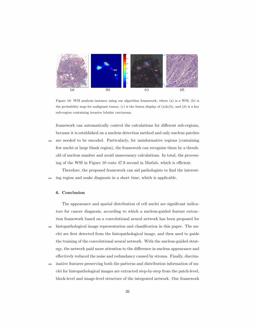
image-level feature and the lesion was predicted. Figure 10 is a 2-class (benign

and malignant tumor) prediction instance, where Figure 10(a) is a WSI with a

size 14K×15K pixels under a 20× lens. We use a 1536 × 1024 sliding-window425

(the step length is 320 pixel) to process the WSI and predict the probability of

malignant tumor for each region. Figure 10(b) is the prediction result, where

red denotes that the probability of the malignancy is 1, and blue denotes the

probability is 0. The probability gradually increases from blue to red. Obviously,

four regions are predicted to have high malignant probability in the WSI. Figure430

10(d) is the display for the region with high malignant probability under high

resolution, where the blue line is the annotation of invasive lobular carcinoma

from pathologists. Thus, using our prediction result, pathologists can fast find

the informative regions from a WSI and make more accurate diagnosis.

Because the nucleus detection and block-level feature extraction are only cal-435

culated one time for the entire WSI, the redundant computation in the overlap-

ping regions between sliding windows can be avoided. In addition, the proposed

25

(a) (b) (c) (d)

Figure 10: WSI analysis instance using our algorithm framework, where (a) is a WSI, (b) is

the probability map for malignant tumor, (c) is the fusion display of (a)&(b), and (d) is a key

sub-region containing invasive lobular carcinoma.

framework can automatically control the calculations for different sub-regions,

because it is established on a nucleus detection method and only nucleus patches

are needed to be encoded. Particularly, for uninformative regions (containing440

few nuclei or large blank region), the framework can recognize them by a thresh-

old of nucleus number and avoid unnecessary calculations. In total, the process-

ing of the WSI in Figure 10 costs 47.9 second in Matlab, which is efficient.

Therefore, the proposed framework can aid pathologists to find the interest-

ing region and make diagnosis in a short time, which is applicable.445

6. Conclusion

The appearance and spatial distribution of cell nuclei are significant indica-

tors for cancer diagnosis, according to which a nucleus-guided feature extrac-

tion framework based on a convolutional neural network has been proposed for

histopathological image representation and classification in this paper. The nu-450

clei are first detected from the histopathological image, and then used to guide

the training of the convolutional neural network. With the nucleus-guided strat-

egy, the network paid more attention to the difference in nucleus appearance and

effectively reduced the noise and redundancy caused by stroma. Finally, discrim-

inative features preserving both the patterns and distribution information of nu-455

clei for histopathological images are extracted step-by-step from the patch-level,

block-level and image-level structure of the integrated network. Our framework

26

is evaluated on a breast-lesion database. The experiment results have certified

that the proposed features are effective to represent histopathological images.

And, the proposed framework achieved the best classification performance in460

classification of breast lesions compared with other state-of-the-art methods.

Further work will focus on clinical applications employing the proposed fea-

tures, such as whole slide image analysis and content-based histopathological

image retrieval.

Acknowledgement465

This work was supported by the National Natural Science Foundation of

China (No. 61371134 and 61471016) and project of Motic-BUAA Image Tech-

nology Research and Development Center.

References

[1] R. L. Siegel, K. D. Miller, A. Jemal, Cancer statistics, 2017, CA: a cancer470

journal for clinicians 67 (1) (2017) online.

[2] S. Zhang, D. Metaxas, Large-scale medical image analytics: Recent

methodologies, applications and future directions, Medical Image Analy-

sis 33 (2016) 98–101.

[3] J. Wu, X. Sun, J. Wang, Y. Cui, F. Kato, H. Shirato, D. M. Ikeda, R. Li,475

Identifying relations between imaging phenotypes and molecular subtypes

of breast cancer: Model discovery and external validation, Journal of Mag-

netic Resonance Imaging in press (2017) online.

[4] J. Wu, Y. Cui, X. Sun, G. Cao, B. Li, D. M. Ikeda, A. W. Kurian, R. Li,

Unsupervised clustering of quantitative image phenotypes reveals breast480

cancer subtypes with distinct prognoses and molecular pathways, Clinical

Cancer Research in press (2017) online.

[5] S. L. Robbins, V. Kumar, A. K. Abbas, N. Fausto, J. C. Aster, Robbins

and Cotran pathologic basis of disease, Saunders/Elsevier, 2010.

27

[6] C. Mosquera-Lopez, S. Agaian, A. Velez-Hoyos, I. Thompson, Computer-485

aided prostate cancer diagnosis from digitized histopathology: A review on

texture-based systems, IEEE Reviews in Biomedical Engineering 8 (2014)

98–113. doi:10.1109/RBME.2014.2340401.

[7] J. S. Duncan, N. Ayache, Medical image analysis: Progress over two

decades and the challenges ahead, IEEE Transactions on Pattern Analysis490

and Machine Intelligence 22 (1) (2000) 85–106. doi:10.1109/34.824822.

[8] M. N. Gurcan, L. E. Boucheron, A. Can, A. Madabhushi, N. M. Rajpoot,

B. Yener, Histopathological image analysis: a review, IEEE Reviews in

Biomedical Engineering 2 (2009) 147–171.

[9] B. E. Bejnordi, M. Balkenhol, G. Litjens, R. Holland, P. Bult, N. Karsse-495

meijer, J. A. W. M. V. Der Laak, Automated detection of dcis in whole-slide

h&e stained breast histopathology images, IEEE Transactions on Medical

Imaging 35 (9) (2016) 2141–2150.

[10] S. R. Lakhani, I. A. for Research on Cancer, W. H. Organization, et al.,

WHO classification of tumours of the breast, International Agency for Re-500

search on Cancer, 2012.

[11] J. C. Caicedo, A. Cruz, F. A. Gonzalez, Histopathology image classifi-

cation using bag of features and kernel functions, in: Artificial intelli-

gence in medicine in europe, Springer, 2009, pp. 126–135. doi:10.1007/

978-3-642-02976-9_17.505

[12] O. Sertel, J. Kong, H. Shimada, U. Catalyurek, J. H. Saltz, M. N. Gur-

can, Computer-aided prognosis of neuroblastoma on whole-slide images:

Classification of stromal development, Pattern recognition 42 (6) (2009)

1093–1103. doi:doi:10.1016/j.patcog.2008.08.027.

[13] E. Mercan, S. Aksoy, L. G. Shapiro, D. L. Weaver, T. Brunye, J. G. Elmore,510

Localization of diagnostically relevant regions of interest in whole slide

28

images, in: International conference on pattern recognition, 2014, pp. 1179–

1184. doi:10.1109/ICPR.2014.212.

[14] Y. Xu, J.-Y. Zhu, I. Eric, C. Chang, M. Lai, Z. Tu, Weakly supervised

histopathology cancer image segmentation and classification, Medical im-515

age analysis 18 (3) (2014) 591–604. doi:10.1016/j.media.2014.01.010.

[15] D. G. Lowe, Distinctive image features from scale-invariant keypoints, In-

ternational Journal of Computer Vision 60 (60) (2004) 91–110.

[16] N. Dalal, B. Triggs, Histograms of oriented gradients for human detection,

in: IEEE Conference on Computer Vision and Pattern Recognition, 2005,520

pp. 886–893.

[17] T. Ojala, I. Harwood, A comparative study of texture measures with clas-

sification based on feature distributions, Pattern Recognition 29 (1) (1996)

51–59.

[18] M. M. Dundar, S. Badve, G. Bilgin, V. Raykar, R. Jain, O. Sertel, M. N.525

Gurcan, Computerized classification of intraductal breast lesions using

histopathological images, IEEE Transactions on Biomedical Engineering

58 (7) (2011) 1977–1984.

[19] M. Kowal, P. Filipczuk, A. Obuchowicz, J. Korbicz, R. Monczak,

Computer-aided diagnosis of breast cancer based on fine needle biopsy530

microscopic images, Computers in biology and medicine 43 (10) (2013)

1563–1572. doi:10.1016/j.compbiomed.2013.08.003.

[20] L. Cheng, M. Mandal, Automated analysis and diagnosis of skin melanoma

on whole slide histopathological images, Pattern Recognition 48 (8) (2015)

27382750. doi:doi:10.1016/j.patcog.2015.02.023.535

[21] S. Doyle, S. Agner, A. Madabhushi, M. Feldman, J. Tomaszewski, Au-

tomated grading of breast cancer histopathology using spectral clustering

with textural and architectural image features, in: IEEE International Sym-

posium on Biomedical Imaging, IEEE, 2008, pp. 496–499.

29

[22] A. N. Basavanhally, S. Ganesan, S. Agner, J. P. Monaco, M. D. Feldman,540

J. E. Tomaszewski, G. Bhanot, A. Madabhushi, Computerized image-based

detection and grading of lymphocytic infiltration in her2+ breast can-

cer histopathology, IEEE Transactions on Biomedical Engineering 57 (3)

(2010) 642–653. doi:10.1109/TBME.2009.2035305.

[23] A. Tabesh, M. Teverovskiy, H.-Y. Pang, V. P. Kumar, D. Verbel, A. Kot-545

sianti, O. Saidi, Multifeature prostate cancer diagnosis and gleason grad-

ing of histological images, IEEE Transactions on Medical Imaging 26 (10)

(2007) 1366–1378.

[24] O. S. Al-Kadi, Texture measures combination for improved meningioma

classification of histopathological images, Pattern recognition 43 (6) (2010)550

2043–2053. doi:10.1016/j.patcog.2010.01.005.

[25] E. Ozdemir, C. Gunduz-Demir, A hybrid classification model for digital

pathology using structural and statistical pattern recognition, IEEE Trans-

actions on Medical Imaging 32 (2) (2013) 474–483.

[26] Y. Zheng, Z. Jiang, J. Shi, Y. Ma, Retrieval of pathology image for breast555

cancer using plsa model based on texture and pathological features, in:

IEEE International Conference on Image Processing, 2014, pp. 2304–2308.

doi:10.1109/ICIP.2014.7025467.

[27] M. Kandemir, F. A. Hamprecht, Computer-aided diagnosis from weak su-

pervision: A benchmarking study, Computerized Medical Imaging and560

Graphics 42 (2015) 44–50. doi:doi:10.1016/j.compmedimag.2014.11.

010.

[28] X. Zhang, H. Dou, T. Ju, J. Xu, S. Zhang, Fusing heterogeneous features

from stacked sparse autoencoder for histopathological image analysis, IEEE

Journal of Biomedical and Health Informatics 20 (5) (2015) 1377–1383.565

[29] Y. Ma, Z. Jiang, H. Zhang, F. Xie, Y. Zheng, H. Shi, Y. Zhao, Breast

30

histopathological image retrieval based on latent dirichlet allocation, IEEE

Journal of Biomedical and Health Informatics PP (99).

[30] A. A. Cruz-Roa, J. E. A. Ovalle, A. Madabhushi, F. A. G. Osorio, A

deep learning architecture for image representation, visual interpretability570

and automated basal-cell carcinoma cancer detection, in: Medical Image

Computing and Computer-Assisted Intervention, Springer, 2013, pp. 403–

410.

[31] J. Arevalo, A. Cruz-Roa, V. Arias, E. Romero, F. A. Gonzalez, An unsuper-

vised feature learning framework for basal cell carcinoma image analysis,575

Artificial intelligence in medicine 64 (2) (2015) 131–145.

[32] J. Xu, L. Xiang, Q. Liu, H. Gilmore, J. Wu, J. Tang, A. Madabhushi,

Stacked sparse autoencoder (ssae) for nuclei detection on breast can-

cer histopathology images, IEEE Transactions on Medical Imagingdoi:

10.1109/TMI.2015.2458702.580

[33] N. Nayak, H. Chang, A. Borowsky, P. Spellman, B. Parvin, Classifi-

cation of tumor histopathology via sparse feature learning, in: Inter-

national Symposium on Biomedical Imaging, IEEE, 2013, pp. 410–413.

doi:10.1109/ISBI.2013.6556782.

[34] H. Chang, N. Nayak, P. T. Spellman, B. Parvin, Characterization of tis-585

sue histopathology via predictive sparse decomposition and spatial pyramid

matching, in: Medical Image Computing and Computer-Assisted Interven-

tion, Springer, 2013, pp. 91–98.

[35] Y. Zhou, H. Chang, K. Barner, P. Spellman, B. Parvin, Classification of

histology sections via multispectral convolutional sparse coding, in: IEEE590

Conference on Computer Vision and Pattern Recognition, IEEE, 2014, pp.

3081–3088.

[36] U. Srinivas, H. S. Mousavi, V. Monga, A. Hattel, B. Jayarao, Simultaneous

31

sparsity model for histopathological image representation and classification,

Medical Imaging, IEEE Transactions on 33 (5) (2014) 1163–1179.595

[37] T. Vu, H. Mousavi, V. Monga, G. Rao, A. Rao, Histopathological im-

age classification using discriminative feature-oriented dictionary learning,

Medical Imaging, IEEE Transactions on 35 (3) (2016) 738–751.

[38] C. Malon, M. Miller, H. C. Burger, E. Cosatto, H. P. Graf, Identifying

histological elements with convolutional neural networks, in: Proceedings600

of the 5th international conference on Soft computing as transdisciplinary

science and technology, ACM, 2008, pp. 450–456.

[39] J. Xu, X. Luo, G. Wang, H. Gilmore, A. Madabhushi, A deep convolutional

neural network for segmenting and classifying epithelial and stromal regions

in histopathological images, Neurocomputing 191 (2016) 214–223.605

[40] L. Hou, D. Samaras, T. M. Kurc, Y. Gao, J. E. Davis, J. H. Saltz, Patch-

based convolutional neural network for whole slide tissue image classifica-

tion, in: IEEE Conference on Computer Vision and Pattern Recognition,

2015, pp. 2424–2433.

[41] X. Zhang, H. Su, L. Yang, S. Zhang, Fine-grained histopathological image610

analysis via robust segmentation and large-scale retrieval, in: Proceedings

of the IEEE Conference on Computer Vision and Pattern Recognition,

2015, pp. 5361–5368. doi:10.1109/CVPR.2015.7299174.

[42] X. Zhang, F. Xing, H. Su, L. Yang, S. Zhang, High-throughput histopatho-

logical image analysis via robust cell segmentation and hashing, Medical615

image analysis 26 (1) (2015) 306–315.

[43] D. Zink, A. H. Fischer, J. A. Nickerson, Nuclear structure in cancer cells,

Nature Reviews Cancer 4 (9) (2004) 677–687.

[44] A. C. Ruifrok, D. A. Johnston, Quantification of histochemical staining

by color deconvolution, Analytical and quantitative cytology and histology620

23 (4) (2001) 291–299.

32

[45] A. Coates, A. Y. Ng, H. Lee, An analysis of single-layer networks in unsu-

pervised feature learning, in: International conference on artificial intelli-

gence and statistics, 2011, pp. 215–223.

[46] J. Masci, U. Meier, D. Ciresan, J. Schmidhuber, Stacked convolutional625

auto-encoders for hierarchical feature extraction, in: International Con-

ference on Artificial Neural Networks, Springer, 2011, pp. 52–59. doi:

10.1007/978-3-642-21735-7_7.

[47] A. Ng, Sparse autoencoder, CS294A Lecture notes 72 (2011) 1–19.

[48] R. H. Byrd, P. Lu, J. Nocedal, C. Zhu, A limited memory algorithm for630

bound constrained optimization, SIAM Journal on Scientific Computing

16 (5) (1995) 1190–1208.

[49] R. Kohavi, et al., A study of cross-validation and bootstrap for accuracy

estimation and model selection, in: Ijcai, 1995, pp. 1137–1145.

[50] A. Krizhevsky, I. Sutskever, G. E. Hinton, Imagenet classification with635

deep convolutional neural networks, in: International Conference on Neural

Information Processing Systems, 2012, pp. 1097–1105.

33