Feasibility study on laser microwelding and laser shock peening using femtosecondlaser pulses

by

Dongkyun Lee

A dissertation submitted in partial fulfillmentof the requirements for the degree of

Doctor of Philosophy(Mechanical Engineering)

in The University of Michigan2008

Doctoral Committee:

Professor Elijah Kannatey-Asibu Jr., ChairProfessor Amit GhoshProfessor Jyotirmoy MazumderProfessor Jwo Pan

Dongkyun Leec© 2008

All rights reserved.

To my parents

ii

Acknowledgements

I express my sincere gratitude and respect to my supervisor, professor Elijah

Kannatey-Asibu Jr. for his great inspiration and gentle guidance during my doctoral

study in the University of Michigan, Ann Arbor.

I also express my special appreciation to professor Amit Ghosh, Jyotirmoy Mazumder

and Jwo Pan for their generous suggestions on my research.

I appreciate Department of Mechanical Engineering for appointing me as a grad-

uate student instructor. It was wonderful experience to meet undergraduate students

in classes for several terms, together with professor Huei Peng, Steve Ceccio, Ann

Marie Sastry, Kevin Pipe and Katsuo Kurabayashi.

I also appreciate John Nees, research scientist in CUOS, the University of Michi-

gan, for his valuable instructions on femtosecond laser system, and professor Jinho

Lee, Kwang-Min Chun, and Hyung-Hee Cho at Yonsei University, Korea, for their

encouragement of starting my doctoral research.

I am indebted to my friends, seniors, juniors and research group members of

professor Kannatey-Asibu for achieving this work, and I thank all of them.

Finally, my special thanks go to my parents in Korea for their full understanding

and support during my doctoral study, and my brother and his wife, my sister and

her husband.

iii

Table of Contents

Dedication . . . . . . . . . . . . . . . . . . . . . . . . . . . . . . . . . . . . . ii

Acknowledgements . . . . . . . . . . . . . . . . . . . . . . . . . . . . . . . iii

List of Figures . . . . . . . . . . . . . . . . . . . . . . . . . . . . . . . . . . vi

List of Tables . . . . . . . . . . . . . . . . . . . . . . . . . . . . . . . . . . . x

List of Appendices . . . . . . . . . . . . . . . . . . . . . . . . . . . . . . . . xii

List of Symbols . . . . . . . . . . . . . . . . . . . . . . . . . . . . . . . . . . xiii

Abstract . . . . . . . . . . . . . . . . . . . . . . . . . . . . . . . . . . . . . . xvi

Chapter

I. Introduction . . . . . . . . . . . . . . . . . . . . . . . . . . . . . . 1

II. Implementation of the two temperature model in ABAQUS 5

2.1 Introduction . . . . . . . . . . . . . . . . . . . . . . . . . . . 52.2 Background . . . . . . . . . . . . . . . . . . . . . . . . . . . . 72.3 Analysis . . . . . . . . . . . . . . . . . . . . . . . . . . . . . . 8

2.3.1 The TTM implementation in ABAQUS . . . . . . . 82.3.2 Temperature dependent terms & material ablation in

ABAQUS . . . . . . . . . . . . . . . . . . . . . . . . 122.3.3 Analytical solutions for the linear TTM . . . . . . . 14

2.4 Results and discussion . . . . . . . . . . . . . . . . . . . . . . 172.4.1 Concept validity check: comparison with Linear TTM

solution . . . . . . . . . . . . . . . . . . . . . . . . . 172.4.2 Nonlinear case of low fluence input & hybrid element

configuration . . . . . . . . . . . . . . . . . . . . . . 192.4.3 Nonlinear case of high fluence input & feasibility of

microwelding with UFL . . . . . . . . . . . . . . . . 252.5 Conclusions . . . . . . . . . . . . . . . . . . . . . . . . . . . . 30

iv

III. Numerical analysis on the feasibility of laser microwelding ofmetals by femtosecond laser pulses using ABAQUS . . . . . . 32

3.1 Introduction . . . . . . . . . . . . . . . . . . . . . . . . . . . 323.2 Background . . . . . . . . . . . . . . . . . . . . . . . . . . . . 333.3 Analysis . . . . . . . . . . . . . . . . . . . . . . . . . . . . . . 36

3.3.1 Overview of the TTM implementation in ABAQUS 363.3.2 Evaluation of temperature dependent material prop-

erties . . . . . . . . . . . . . . . . . . . . . . . . . . 393.4 Results and discussion . . . . . . . . . . . . . . . . . . . . . . 43

3.4.1 Feasibility of LMW with UFL - multiple pulses . . . 433.4.2 Feasibility of LMW with UFL - pulse duration . . . 473.4.3 Feasibility of LMW with UFL - focal radius . . . . . 52

3.5 Conclusions . . . . . . . . . . . . . . . . . . . . . . . . . . . . 55

IV. Experimental investigation of laser shock peening using fem-tosecond laser pulses . . . . . . . . . . . . . . . . . . . . . . . . . 57

4.1 Introduction . . . . . . . . . . . . . . . . . . . . . . . . . . . 574.2 Background . . . . . . . . . . . . . . . . . . . . . . . . . . . . 594.3 Experiment . . . . . . . . . . . . . . . . . . . . . . . . . . . . 614.4 Results and discussion . . . . . . . . . . . . . . . . . . . . . . 644.5 Summary . . . . . . . . . . . . . . . . . . . . . . . . . . . . . 73

V. Conclusions and Future work . . . . . . . . . . . . . . . . . . . . 74

Appendices . . . . . . . . . . . . . . . . . . . . . . . . . . . . . . . . . . . . 77

Bibliography . . . . . . . . . . . . . . . . . . . . . . . . . . . . . . . . . . . 87

v

List of Figures

Figure

2.1 The concept of dual domain configuration for the TTM in ABAQUS 9

2.2 (a) Temperature information sharing via common memory block inthe user subroutine, USDFLD, shown as USD in the figure: The ♦

marks indicate that the subroutine is called at the integration pointsof 4-node planar elements, Ωn

e and Ωml (b) Effective heat capacity with

the latent heat (Area B) for phase change in USDFLD . . . . . . . . 13

2.3 4-node linear planar finite element: (a) actual coordinates, and (b)normalized coordinates . . . . . . . . . . . . . . . . . . . . . . . . . 14

2.4 A dual domain setup of the TTM implementation for ABAQUS (Lx

= 200 nm, ∆x = 1 nm) . . . . . . . . . . . . . . . . . . . . . . . . . 18

2.5 (a) lattice temperature histories at the top surface for heat sourcesof different temporal profiles, and (b) corresponding temperature dis-tributions at select times; (c) lattice temperature histories at the topsurface for heat sources of different spatial distributions, and (d) cor-responding temperature distributions at select times: the legend label“FEM” stands for results from ABAQUS, “Analytic” for results fromanalytical series solutions . . . . . . . . . . . . . . . . . . . . . . . . 20

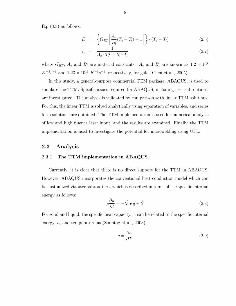
2.6 Normalized homogeneous electron temperature histories for a laserpulse of tp = 96 fs at the top and back surface for different materialthicknesses of (a) 100 nm, and (b) 200 nm. Data set “QT” taken fromQiu and Tien (1993). In the legend, dt stands for ∆t, and tp for tp . 23

2.7 Temperature distributions inside a material (Lx = 100 nm) for a laserpulse of tp = 100 fs at select times: (a) electron temperature, and (b)lattice temperature. Data set “QT” taken from Qiu and Tien (1993).In the legend, dt stands for ∆t, and tp for tp . . . . . . . . . . . . . 24

vi

2.8 (a) Homogeneous and (b) hybrid element configurations (Lx = 200 nm) 24

2.9 Comparison of FEM results for homogeneous and hybrid elements: (a)electron and lattice temperature histories at select locations, and (b)electron and lattice temperature distributions at select times. Marksin (b) represent the locations of nodes . . . . . . . . . . . . . . . . . 25

2.10 (a) Lattice temperatures at the top surface and ablation depth histo-ries (b) Lattice temperature distributions for t = 2.0 and 22.0 ps, J= 800 mJ/cm2. In the legends, dT stands for ∆Tm, dt for ∆t . . . . 27

2.11 (a) Ablation depth with respect to the input fluence. Data set “CLB”taken from Chen et al. (2005), and “Exp” from Preuss et al. (1995).(b) Corresponding ablation starting and ending time, and averageablation rate with respect to the input fluence . . . . . . . . . . . . 28

2.12 (a) Molten pool depth change history traced with melting point forselect fluences (b) Estimation on molten pool thickness traced withmelting point (Tm in the legend) and the liquidus (Tm+dT in thelegend), with respect to the input fluence . . . . . . . . . . . . . . . 29

3.1 A dual domain configuration for the TTM in ABAQUS . . . . . . . 37

3.2 Overall workflow of ABAQUS user subroutines for the TTM imple-mentation: USD stands for USDFLD, UMTH for UMATHT, andUMM for UMESHMOTION . . . . . . . . . . . . . . . . . . . . . . 38

3.3 (a) Chemical potentials evaluated for DOS with s and d electrons ands electron only configurations (b) Curve-fitted G(Te) and Ce(Te) withoriginal values; Ce(Te) of linear model (Ce = γ · Te) is also plotted.For the Te axis, “[X 1000 K]”, indicates that the number on the axisshould be multiplied by 1000 for the exact value of K, i.e., “40” in (a)should read 40000 K. . . . . . . . . . . . . . . . . . . . . . . . . . . 40

3.4 1D dual domain configuration of TTM implementation for ABAQUS 43

3.5 (a) Ablation depth with respect to input fluence. Data set “Exp”taken from Preuss et al. (1995), and “CB” from Chen and Beraun(2003). (b) Maximum molten pool thickness and ablation depth withrespect to input fluence . . . . . . . . . . . . . . . . . . . . . . . . . 45

vii

3.6 (a) Lattice temperature histories at the top surface for select pulserepetition rates. (b) Maximum relative molten pool and ablationthicknesses with respect to repetition rates. In the figure, pulse du-ration is 500 fs. . . . . . . . . . . . . . . . . . . . . . . . . . . . . . 47

3.7 (a) Ablation threshold fluence with respect to pulse duration. Ex-perimental data set “Exp” taken from Furusawa et al. (1999). (b)Ablation histories at the top surface for select pulse durations with J= 4 J/cm2. . . . . . . . . . . . . . . . . . . . . . . . . . . . . . . . . 48

3.8 (a) Maximum molten pool thickness with respect to input fluence forselect pulse durations. (b) Corresponding molten pool thickness andablation depth with respect to pulse duration . . . . . . . . . . . . . 49

3.9 Lattice temperature distributions at select times with fluence of 8J/cm2 for pulse duration of (a) 1 ps, and (b) 100 ps; Horizontal dot-dashed line in both figures represents the melting point. . . . . . . . 50

3.10 (a) Difference between maximum electron and lattice temperature forselect fluences with respect to pulse duration, and corresponding rela-tive time delay between electron and lattice maximum temperatures;in the figure, “Te,max” and “Tl,max” represent Te,max and Tl,max, re-spectively. (b) Comparison of temperature histories at the top andbottom surface evaluated from the TTM and conventional heat con-duction model (denoted as “OTM” in the legend) for tp = 5 ns, J =8 J/cm2; in the figure, Te and Tl represent Te and Tl, respectively. . 51

3.11 (a) Axisymmetric 3D dual domain configuration. (b) Ablated topsurface (z = 0) profile for select focal radii and fluences. Note thatunit length scales are different for depth and radius coordinates. . . 53

3.12 Molten pool edge and top surface profile developed by a beam radiusof rf = 0.5 µm at select times for (a) J = 800 mJ/cm2 and tp = 0.5ps, and for (b) J = 400 mJ/cm2 and tp = 500 ps; Comparison ofmolten pool edges developed by select beam focal radii at the timesof maximum depths for (c) select fluences and tp = 0.5 ps, and (d)select pulse durations and J = 400 mJ/cm2 . . . . . . . . . . . . . . 54

4.1 A water confined configuration for laser shock peening . . . . . . . . 59

4.2 (a) Overall layout of experimental set-up (b) A focused UFL forminga visible spot in air . . . . . . . . . . . . . . . . . . . . . . . . . . . 61

viii

4.3 (a) Two examples of microscope photos for single line scanning on thetop surface of galvanized steel specimen. (b) Scanning pattern on thetop surface of a specimen. . . . . . . . . . . . . . . . . . . . . . . . . 62

4.4 Sections of (a) galvanized, and (b) galvannealed steel specimens. Spec-imens were sectioned, cold mounted, polished and etched using 0.5%nitol (Vander Voort, 2004). . . . . . . . . . . . . . . . . . . . . . . . 63

4.5 Experimental data comparison of galvanized steel specimens for selectfeed rates, f = 500 and 1000 µm/s, with respect to input fluence: (a)Microhardness. (b) Maximum depth of the processed region. In thefigure, “um” represents µm. . . . . . . . . . . . . . . . . . . . . . . . 65

4.6 Section of galvanized steel specimen after LSP with J = 5.43 J/cm2

for feed rate of (a) 500 µm/s and (b) 50 µm/s . . . . . . . . . . . . 66

4.7 Debris generated during galvanized steel experiment: (a) Before and(b) after the experiment . . . . . . . . . . . . . . . . . . . . . . . . . 66

4.8 Experimental data comparison of galvanized and galvannealed steelspecimens for feed rate f = 500 µm/s, with respect to input fluence:(a) Microhardness. (b) Maximum depth of the processed region. Inthe figure, “um” represents µm. . . . . . . . . . . . . . . . . . . . . 68

4.9 Two possibilities on a relation between UFL input fluence and hard-ness at top surface of base material: (a) no change in hardness, and(b) hardening effect. In the figure, “Hv” and “J” represent the mi-crohardness and input fluence, respectively. . . . . . . . . . . . . . . 69

4.10 Top surface of shock peened specimens for select fluences for (a) galva-nized, and (b) galvannealed steel: In the figure, J1 = 0.09, J2 = 0.21,J3 = 1.73 and J4 = 5.43 J/cm2. “Original” indicates top surfaceswithout LSP. . . . . . . . . . . . . . . . . . . . . . . . . . . . . . . . 72

ix

List of Tables

Table

2.1 Material properties of gold at ambient temperature . . . . . . . . . . 19

2.2 Parameters for low fluence case study (Qiu and Tien, 1993) . . . . . 22

2.3 Hybrid element configurations for the thickness of 200 and 1000 nm 24

2.4 Material properties of Gold for high fluence case study (Chen et al.,2005) . . . . . . . . . . . . . . . . . . . . . . . . . . . . . . . . . . . 26

3.1 The updating relations for internal energy and heat flux related termsin the user subroutine UMATHT . . . . . . . . . . . . . . . . . . . . 37

3.2 Coefficients of piecewise curve-fitting functions of Eqs. (3.12) and (3.13) 41

3.3 Constants used for the material model and problem set-up . . . . . 44

4.1 Thermal properties (Mills, 1992) of select materials . . . . . . . . . . 60

4.2 Labeled and measured optical densities (OD) of neutral density filtersand corresponding fluences calculated from J = 10−OD·J0, where J0 =5.43 J/cm2 . . . . . . . . . . . . . . . . . . . . . . . . . . . . . . . . 63

4.3 Chemical composition (wt%) of an AKDQ steel (Zhang and Senkara,2006) . . . . . . . . . . . . . . . . . . . . . . . . . . . . . . . . . . . 63

4.4 ANOVA table of data for galvanized steel. In the table, “DoF” standsfor degree of freedom. “Fcrit” is the critical F ratio for a given degreeof freedom. Levels for the factors J and f are 0.09, 0.21, 1.73 and5.43 J/cm2, and 500 and 1000 µm/s, respectively. . . . . . . . . . . 67

x

4.5 Hardness increment for laser peening processes on steels. The esti-mated increment for this study is also listed . . . . . . . . . . . . . . 70

xi

List of Appendices

Appendix

A. Derivation of the energy term updating equation . . . . . . . . . . . 78

B. Derivation of the heat flux term updating equation . . . . . . . . . . 80

C. Source codes of ABAQUS user subroutines . . . . . . . . . . . . . . . 82

xii

List of Symbols

c, C = specific and volumetric bulk heat capacity, respectively. C in [J m−3

K−1]

ce, Ce = specific and volumetric electron heat capacity, respectively; Ce(= ρce) in

[J m−3 K−1]

cl, Cl = specific and volumetric lattice heat capacity, respectively; Cl(= ρcl) in

[J m−3 K−1]

D(ε) = density of state (DOS) of free electrons [eV−1]

dab, dm = the maximum depth of ablation and melting, respectively [nm]

E = coupling energy between the electrons and the lattice [J m−3]

fe(ε, Te) = Fermi-Dirac distribution

G = the electron-phonon coupling factor [W m−3 K−1]

Hm = specific latent heat [J kg−1]

Hv = heat of evaporation [J kg−1]

! = 1.05459 × 10−34 [J · s], Planck’s constant

J = laser input fluence [J cm−2]

Jab, Jm = ablation and melting threshold fluence, respectively [J cm−2]

k = thermal conductivity [W m−1 K−1]

kB = 1.3807 × 10−23 [J K−1], Boltzmann’s constant

ke, kl = electron and lattice thermal conductivity, respectively [W m−1 K−1]

keq = thermal conductivity at equilibrium state (Te = Tl) [W m−1 K−1]

L, Lx = length scales and a domain size, respectively [nm]

l, m, n = index numbers (0, 1, 2, 3 . . . ) for analytical series solutions

me = electron mass [kg]

xiii

N = number density of electrons [m−3]

Pb = boiling pressure [kPa]

q, $q = heat flux [W m−2]

R = reflectivity of the material

$rBC = a location vector of a domain boundary

rf = focal radius [nm]

S, S($r, t) = a heat source term [W m−3]

S ($ξ, τ) = heat source term in dimensionless coordinates

T ($ξ, τ) = temperature in dimensionless coordinates

T , Tl = (lattice) temperature [K]

Tb(Pb) = boiling point of a material at given pressure, Pb [K]

Te = electron temperature [K]

TF = Fermi temperature [K]

Tlq = Tm + ∆Tm, liquidus [K]

Tm = melting point [K]

∆Tm = solidification temperature [K]

Tnorm = normalization temperature for analytical solutions [K]

Tso = Tm − ∆Tm, solidus [K]

Ttop = temperature at the top surface of a material [K]

T∞, T0 = ambient and initial temperature, respectively (constant) [K]

tp = pulse duration in FWHM [ps]

u, U = specific and volumetric internal energy, respectively; U(= ρu) in [J m−3]

u(t) = unit step function

Vs = speed of sound [m s−1]

x = coordinate in depth direction in 1D [nm]

αs = coefficient for the subsurface boiling ablation model

γe = ce/c, dimensionless electron heat capacity

γl = cl/c, dimensionless lattice heat capacity

δ(t) = Dirac delta function

δs = skin depth [nm]

xiv

εF = kB · TF , Fermi energy [eV]

ε = k/(GL2), dimensionless electron-phonon coupling factor

θm = dm − dab, the maximum molten pool thickness [nm]

ϑ = (T ($ξ, τ) − T∞)/(Tnorm − T∞),normalized dimensionless temperature

κ = k/ρc, thermal diffusivity [m2 s−1]

λ = wavelength [nm]

λe = electron-phonon coupling constant (dimensionless)

Ξx,y,z = Lx,y,z/L, dimensionless length scale

$ξ = $r/L, dimensionless location vector

ρ = mass density [kg m−3]

ς = S ($ξ, τ)/(k · (Tnorm − T∞)/L2), dimensionless heat source

τ = t · (k/ρc)/L2, dimensionless time

τe = electron relaxation time [ps]

Ωne , Ωm

l = n-th element in electron domain, and m-th element in lattice domain

〈ω2〉 = second moment of the phonon spectrum [meV2]

xv

Abstract

Ultrafast lasers of sub-picosecond pulse duration have thus far been investigated

for ablation, drilling and cutting processes. Ultrafast lasers also have the potential

for laser welding of small components of the order of microns, and for laser shock

peening to enhance the peening depth.

First, the two-temperature model is implemented in a general-purpose commercial

FEM package, ABAQUS, to enable broad based application of the two-temperature

model in practical engineering problems. The implementation is validated by com-

parison with linear solutions obtained using separation of variables. It is then used

to investigate the potential for microwelding using an ultrafast laser pulse.

Next, the two-temperature model is analyzed using ABAQUS to study the feasibil-

ity of laser microwelding with ultrafast lasers. A material model is constructed using

material properties and the subsurface boiling model for ablation. Laser processing

parameters of repetition rate, pulse duration, and focal radius are then investigated,

in terms of molten pool generated in the material, and requirements for those param-

eters are discussed to obtain feasible parameter ranges for laser microwelding using

ultrafast lasers.

Then, the feasibility of laser shock peening using ultrafast laser pulses was ex-

perimentally investigated. A zinc coating was used for the thermo-protective effect,

and a water confining layer was considered in the investigation. A high numerical

aperture focusing lens was used to avoid optical breakdown of the water layer. Laser

fluence and feed rate were selected as experimental parameters. Microhardness mea-

surements were made on the top surface of the shock peened specimen and compared

with the original material hardness. Improvement in microhardness obtained after

laser shock peening with ultrafast laser pulses was slight, compared to results in the

xvi

literature.

Finally, conditions to achieve feasible laser microwelding and laser shock peening

using femtosecond laser pulses are discussed from the numerical and experimental

observations.

xvii

Chapter I

Introduction

Lasers have been used as a tool for precise materials processing in micro and

nano manufacturing operations due to its non-contact nature and the high intensity

resulting from the ability to focus it to a small diameter. Developments in laser

technology have enabled smaller wavelengths, shorter pulse durations, and higher

powers to be achieved, and made it possible for engineers and scientists to perform

an almost unlimited variety of new functions or tasks using lasers (Siegman, 1986).

They have proven to have superior ability in fusion welding of various metals

(Fabbro et al., 2005; Cao et al., 2006; Richter et al., 2007); dissimilar metals (Tri-

antafyllidis et al., 2003; Mys and Schmidt, 2006; Sierra et al., 2007); even dissimilar

non-metallic materials, for example, glass and silicon (Wild et al., 2001). CO2 or

Nd:YAG lasers in continuous wave (CW) mode or with pulse duration of the order

of milliseconds are dominant in the laser welding industry (Kalpakjian and Schmid,

2001). Lasers are considered to be the best choice among a variety of micro-scale

material joining methods (Brockmann et al., 2002). Laser welding of thin foils of

micrometer thickness has been successfully performed (Du et al., 2002; Abe et al.,

2003; Park et al., 2003; Isamu et al., 2004). However, for very small components with

overall dimensions of the order of microns, CW or pulsed lasers currently used for

welding may affect the entire part, and that may not be acceptable. Semak et al.

(2003) indicated that pulse durations shorter than 1 ms may enable microwelding

of fusion zones of the order of or smaller than 100 µm. Duley (2004) mentions the

possibility of extending laser welding technology to nanoscale structures, based on

the notion that it is the geometry of the part itself, and not the wavelength, that

1

2

determines processing efficiency.

Laser shock peening (LSP) has been extensively investigated since the works of

Gregg and Thomas (1966) and Anderholm (1970) were reported. It has been inves-

tigated for various materials, including steel (Peyre et al., 2000; Yilbas et al., 2003;

Yakimets et al., 2004; Aldajah et al., 2005; Farrahi and Ghadbeigi, 2006), aluminum

(Fairand et al., 1972; Peyre et al., 1996; Hong and Chengye, 1998; Rubio-Gonzalez

et al., 2004; Tan et al., 2004) and nickel alloy, molybdenum and copper (Forget et al.,

1990; Hammersley et al., 2000; Kaspar et al., 2000; Zhang et al., 2004). It has also

been successfully applied to improve fatigue life of automotive ring and pinion gears

and aircraft engine turbine blades (See et al., 2002). Laser shock peening is known to

be superior to conventional shot peening for such surface treatment since it results in

deeper compressive residual stresses and smoother processed surface, together with

the capability of localized processing (Montross et al., 2002). Despite significant im-

provements over the years, Fabbro et al. (1998) indicated the potential to improve the

process by adopting extremely short laser pulses to achieve higher pressure, and thus

deeper processed layers. This can be inferred from an experimental demonstration on

acoustic signal generation using short laser pulse durations between 100 fs and 150

ps (Dehoux et al., 2006).

Ultrafast lasers (UFL) of sub-picosecond pulse duration have the potential for over-

coming current limitations of laser welding and shock peening. During laser-matter

interaction for an extremely short pulse energy input to a metal, equilibrium may not

be established between the electrons and lattice because the time required to establish

equilibrium in the electron gas is much less than the time for achieving equilibrium

between the electrons and the lattice (Kaganov et al., 1957). Unfortunately, conven-

tional thermal diffusion models are not adequate for such non-equilibrium conditions.

Even though there have been several models to describe such thermal behavior of

a material (Tzou, 1997), the two-temperature model (TTM) proposed by Anisimov

et al. (1974) has been widely adopted to understand the laser-matter interaction of

ultrashort laser pulses for metals. It describes the interaction in terms of electron and

lattice temperatures, and an electron-phonon coupling factor. The TTM has been

3

used for investigations on laser-mater interaction in the sub-picosecond pulse regime

(Elsayedali et al., 1987; Sherman et al., 1989; Fann et al., 1992; Wellershoff et al.,

1999; Schmidt et al., 2002).

Ultrafast laser technology, for example chirped pulse amplification (Strickland and

Mourou, 1985) has been used to investigate processing applications such as material

ablation, drilling and cutting (Preuss et al., 1995; Momma et al., 1997; Banks et al.,

2000; Griffith et al., 2003). Liu et al. (1997) provided extensive discussion on chirped

pulse amplification (CPA) laser generation technology and its application to laser

material processing. The uniqueness of UFL for material removal over longer pulse

durations has been demonstrated experimentally (Pronko et al., 1995; Chichkov et al.,

1996; Zhu et al., 1999). In recent years, successful microwelding of glasses with

measurable joint strength has been achieved using UFL (Tamaki et al., 2006).

Numerical analysis of laser materials processing has been extensively undertaken.

The finite element method (FEM), including general-purpose commercial FEM pack-

ages such as ABAQUS, is frequently employed for numerical analysis of LSP (Braisted

and Brockman, 1999; Peyre et al., 2003); of welding (Deshayes et al., 2003; Borrisut-

thekul et al., 2005; Lin et al., 2005); and of laser bending (Zhang and Xu, 2003).

However, special purpose codes are usually constructed for numerical analysis involv-

ing the TTM (Qiu and Tien, 1993; Huttner and Rohr, 1996; Chen and Beraun, 2001;

Schmidt et al., 2002).

The goal of this study is to investigate the feasibility of laser microwelding and

laser shock peening using UFL, and the outcomes are described in Chapter 2, 3 and

4.

Chapter 2 covers the TTM implementation in a general-purpose commercial FEM

package, ABAQUS, to enable broad based application of the TTM in practical en-

gineering problems. This chapter has been accepted for publication in the ASME

Journal of Manufacturing Science and Engineering.

Chapter 3 deals with a feasibility study of laser microwelding of metals using UFL.

Select laser parameters of pulse repetition rate, pulse duration and focal radius, are

examined numerically with the TTM implementation of Chapter 2, and requirements

4

on those laser parameters for feasible microwelding of metals with UFL are proposed.

This chapter has been accepted for publication in the ASME Journal of Manufacturing

Science and Engineering.

Chapter 4 describes experimental investigation on the feasibility of laser shock

peening of top coated steel in water confined configuration using ultrafast laser pulses.

This chapter is under preparation for submission to the 27th International Congress

on Applications of Lasers & Electro-Optics (ICALEO) and the Journal of Laser Ap-

plication.

In Chapter 5, conclusions on the feasibility of laser microwelding and laser shock

peening using UFL are drawn from the numerical and experimental studies.

Chapter II

Implementation of the two temperature model in ABAQUS

2.1 Introduction

As a result of their ability to produce high-energy concentrations and be focused to

very small size, lasers have demonstrated their capability as a tool of choice in micro

and nano manufacturing operations. Developments in laser technology have enabled

smaller wavelengths, shorter pulse durations, and higher powers and frequencies to

be achieved, and make it possible for engineers and scientists to perform an almost

unlimited variety of new functions or tasks using lasers (Siegman, 1986). Lasers have

been successfully applied in microfabrication, for example recrystallization, drilling,

trimming, cleaning, welding and surface modification. The most successful of these

applications are microhole drilling, trimming, and recrystallization (Dickinson, 2002).

Thin metal sheets of few tens of microns have been successfully welded using lasers

from CW to milliseconds pulses (Du et al., 2002; Park et al., 2003). Moreover, Semak

et al. (2003) suggest that short pulses should be used to perform microwelding at small

beam diameters of few tens of micrometers. Duley (2004) mentions the possibility

of extending laser welding technology to nanoscale structures, based on the notion

that it is the geometry of the part itself, and not the wavelength, that determines

processing efficiency. However, for very small components with overall dimensions of

the order of microns, CW or pulsed lasers currently used for welding may affect the

entire part, and that may not be acceptable.

Laser shock peening (LSP) has also been extensively investigated since the works

of Gregg and Thomas (1966) and Anderholm (1970) were reported, as summarized by

Fabbro et al. (1998) and Montross et al. (2002). Fabbro et al. (1998) indicated that

5

6

shorter laser pulses can produce higher pressures, resulting in greater shock peening

depth.

Ultrafast lasers (UFL) of sub-picosecond pulse duration have the potential for

overcoming such current limitations of laser welding and shock peening. In laser-

matter interaction for an extremely short pulse energy input to a metal, equilibrium

may not be established between the electrons and lattice because the time required to

establish equilibrium in the electron gas is much less than the time for achieving equi-

librium between the electrons and the lattice (Kaganov et al., 1957). Unfortunately,

conventional thermal diffusion models are not adequate for such non-equilibrium con-

ditions. Thus, Anisimov et al. (1974) proposed the two-temperature model (TTM)

to account for this phenomenon.

Ultrafast laser technology, for example chirped pulse amplification (Strickland and

Mourou, 1985) has been used to investigate processing applications such as material

ablation, drilling and cutting (Preuss et al., 1995; Momma et al., 1997; Banks et al.,

2000; Griffith et al., 2003). Liu et al. (1997) provided extensive discussion on CPA

laser generation technology and its application to laser material processing. The

TTM has also been used for investigations on laser-mater interaction in the sub-

picosecond pulse regime (Elsayedali et al., 1987; Sherman et al., 1989; Fann et al.,

1992; Wellershoff et al., 1999; Schmidt et al., 2002).

Numerical analyses on laser materials processing have also been extensively un-

dertaken. The finite element method (FEM), including general-purpose commercial

FEM packages such as ABAQUS, is frequently employed for numerical analysis of

LSP (Braisted and Brockman, 1999; Peyre et al., 2003); of welding (Deshayes et al.,

2003; Borrisutthekul et al., 2005; Lin et al., 2005); and of laser bending (Zhang and

Xu, 2003). For numerical analysis involving the TTM, special purpose codes have

usually been constructed (Schmidt et al., 2002; Qiu and Tien, 1993; Huttner and

Rohr, 1996; Chen and Beraun, 2001).

The goal of this study is to implement the TTM in a general-purpose commercial

FEM package, ABAQUS, to enable broad based application of the TTM in practical

engineering problems.

7

2.2 Background

Anisimov et al. (1974) proposed the two-temperature model (TTM) as follows:

Ce∂Te

∂t= −$∇ • $qe − E(Te, Tl) + S($s, t) (2.1a)

Cl∂Tl

∂t= E(Te, Tl) (2.1b)

where E(Te, Tl) is given by the following equation, when Te and Tl are much higher

than the Debye temperature:

E(Te, Tl) =π2meNV 2

s

6· (Te − Tl) ≡ G · (Te − Tl) (2.2)

In this model, Ce and Cl are temperature dependent, and Fouriers law is used as a

heat flux model. It is evident from Eq. (3.2) that G is neither a function of electron

nor lattice temperature. Qiu and Tien (1993) incorporated a different heat flux model

based on the Boltzmann transport equation as follows:

τe∂qe

∂t+ qe = −ke

∂Te

∂x(2.3)

where τe is a constant, and the electron thermal conductivity is considered as a

function of the electron and lattice temperatures as follows:

ke = keq ·Te

Tl(2.4)

Anisimov and Rethfeld (1997) further modified the TTM with an additional lattice

thermal conduction term and an electron thermal conductivity that was described as

follows:

ke = χ ·(φ2

e + 0.16)5/4 · (φ2e + 0.44) · φe

(φ2e + 0.092)1/2 · (φ2

e + η · φl)(2.5)

where φe = kBTe/εF and φl = kBTl/εF for the Fermi energy εF (= kB · TF ). χ and η

are material constants, with χ= 353 W/K · m and η = 0.16 for gold. Schmidt et al.

(2002) considered several thermal conductivity models for the TTM with ballistic

electrons and they compared their results with experimental data. Chen et al. (2005)

subsequently introduced a Te and Tl dependent and τe for the heat flux model of

8

Eq. (3.3) as follows:

E =

GRT

[

Ae

Bl(Te + Tl) + 1

]

· (Te − Tl) (2.6)

τe =1

Ae · T 2e + Bl · Tl

(2.7)

where GRT , Ae and Bl are material constants. Ae and Bl are known as 1.2 × 107

K−2s−1 and 1.23 × 1011 K−1s−1, respectively, for gold (Chen et al., 2005).

In this study, a general-purpose commercial FEM package, ABAQUS, is used to

simulate the TTM. Specific issues required for ABAQUS, including user subroutines,

are investigated. The analysis is validated by comparison with linear TTM solutions.

For this, the linear TTM is solved analytically using separation of variables, and series

form solutions are obtained. The TTM implementation is used for numerical analysis

of low and high fluence laser input, and the results are examined. Finally, the TTM

implementation is used to investigate the potential for microwelding using UFL.

2.3 Analysis

2.3.1 The TTM implementation in ABAQUS

Currently, it is clear that there is no direct support for the TTM in ABAQUS.

However, ABAQUS incorporates the conventional heat conduction model which can

be customized via user subroutines, which is described in terms of the specific internal

energy as follows:

ρ∂u

∂t= −$∇ • $q + S (2.8)

For solid and liquid, the specific heat capacity, c, can be related to the specific internal

energy, u, and temperature as (Sonntag et al., 2003):

c =∂u

∂T(2.9)

9

Fig. 2.1. The concept of dual domain configuration for the TTM in ABAQUS

By applying Eq. (2.9) to Eqs. (3.1a) and (3.1b) with relations of Ce = ρce and Cl = ρcl,

the TTM can be rewritten as:

ρ∂ue

∂t= −$∇ • $qe − E + S (2.10a)

ρ∂ul

∂t= E (2.10b)

There is an obvious similarity when Eqs. (2.10a) and (2.10b) are compared with

Eq. (2.8); Equation (2.8) is generally solved within a set of elements, or a domain with

boundary and initial conditions. Thus, the TTM can be modeled for ABAQUS, if two

geometrically independent domains can be established, which are correlated with each

other in terms of thermal behavior of a material, especially for E , as illustrated in

Fig. 2.1, and can be named as a dual domain configuration. The required correlations

can be modeled using user subroutines provided by ABAQUS.

ABAQUS provides a user subroutine UMATHT for modeling customized thermal

behavior of materials (ABAQUS Inc., 2006). In the subroutine, there are six thermal

behavior related variables that should be updated for the next time step t+∆t, based

on the values provided for the current time t. Three of them are closely related to

the internal energy and the other three to heat flux.

First, the three internal energy-related terms, u, ∂u/∂T and ∂u/∂($∇T ) , are

discussed. For the internal energy, u, the heat source term and the electron-phonon

coupling term of the TTM should be considered at the same time when the u term

is updated for the next time step t + δt. With the assumption that the density, ρ,

is not time dependent, Eqs. (2.10a) and (2.10b) can be rearranged in terms of the

10

volumetric internal energy, U , as follows:

Ue + E − S = −$∇ • $qe (2.11a)

Ul − E = 0 (2.11b)

where the upper dots represent partial differentiation with respect to time. From the

left side of Eqs. (2.11a) and (2.11b), effective energy terms for the electron and lattice

system, Ue,eff and Ul,eff , can be defined as Ue,eff ≡ Ue + E − S and Ul,eff ≡ Ul − E.

Then, the effective internal energy terms to be updated for the next time t + ∆t,

U t+∆te,eff and U t+∆t

e,eff , can be written in terms of the current values, U te,eff and U t

l,eff , as

U t+∆te,eff = U t

e,eff + dUe,eff and U t+∆tl,eff = U t

l,eff + dUl,eff . The dUe,eff and dUl,eff terms can

be evaluated mathematically (see Appendix A), which results in the following:

U t+∆te,eff = U t

e,eff +

[(

∂Ue

∂Te

)

· ∆Te + (E − S) ·∆t

]

(2.12a)

U t+∆tl,eff = U t

l,eff +

[(

∂Ul

∂Tl

)

· ∆Tl − E · ∆t

]

(2.12b)

With the exception of the partial derivative terms, the values of E, S, U te,eff and

U tl,eff are all known to the user subroutine. In addition, the equations are written

in discretized form by replacing d with ∆ to indicate that those terms are evaluated

from the finite differences between time t and t + ∆t. The term ∂U/∂T can be easily

found from Eq. (2.9) and the relation U = ρu as follows:

∂Ue

∂Te= ue ·

∂ρ

∂Te+ Ce (2.13a)

∂Ul

∂Tl= ul ·

∂ρ

∂Tl+ Ce (2.13b)

At this point, the density, ρ, is assumed as a constant with respect to Te and Tl

for simplicity. Then the ∂ρ/∂Te and ∂ρ/∂Tl terms vanish from the equations. At

the same time, Eqs. (2.13a) and (2.13b) can be substituted into Eqs. (2.12a) and

(2.12b) to complete their evaluation. In addition, it is assumed that Ue,eff and Ul,eff

are independent of the temperature gradients. Hence, for both electron and lattice

11

internal energy terms, we have

∂Ue

∂$∇Te

= $0 (2.14a)

∂Ul

∂$∇Tl

= $0 (2.14b)

It must be noted that Ce, Cl, E and S in Eqs. (2.12) and (2.13) can be either constant

or functions of variables, including time, location and temperature.

The heat flux related terms, $q, ∂$q/∂T and ∂$q/∂($∇T ), can be obtained from the

heat flux model, for example, Fouriers law or Eq. (3.3). Equation (3.3) is considered

in the following discussion, with a temperature dependent τe, Eq. (3.6). If the first

term on the left side of Eq. 3.3 is discretized over a finite time step ∆t, and the second

term is replaced with a value at the next time step t+∆t, the equation can be written

as follows:

τe

qt+∆te,x − qt

e,x

∆t+ qt+∆t

e,x = −ke ·∂Te

∂x

The temperature gradient term is not discretized because ABAQUS provides the

information to the user subroutine. Then, rearrangement of the equation gives

qt+∆te,x =

1

τe + ∆t·(

τe · qte,x − ∆t · ke ·

∂Te

∂x

)

(2.15)

It should be noted that all the terms on the right side of the equation are known to the

user subroutine, either provided by ABAQUS or the user. The ∂$q/∂T and ∂$q/∂($∇T )

terms can also be obtained in a manner similar to Eq. (2.15) (see Appendix B), and

the results are:(

∂q

∂T

)t+∆t

e,x

=1

τe + ∆t·[

τe ·(

∂q

∂T

)t

e,x

+∂τe

∂Te·

∆t

τe + ∆t·(

ke∂Te

∂x+ qt

e,x

)

− ∆t ·∂ke

∂Te·∂Te

∂x

]

(2.16)

(

∂q

∂(∇T )

)t+∆t

e,x

=1

τe + ∆t·[

τe ·(

∂q

∂(∇T )

)t

e,x

− ∆t · ke

]

(2.17)

Equations (2.15), (2.16) and (2.17) can be modified for Fouriers law, $q = −k · $∇T ,

by setting τe in those equations as zero, as can be seen from Eq. (3.3). In addition,

12

the derivative terms in Eq. (2.16) can be evaluated explicitly from Eq. (2.4) or (2.5)

for ∂ke/∂Te, and (3.6) for ∂τe/∂Te.

2.3.2 Temperature dependent terms & material ablation in ABAQUS

Equations (2.12) to (2.17) should be coded in a user subroutine UMATHT. It is

known that the subroutine is called at integration points of an element. That presents

a technical problem in implementing the TTM in ABAQUS: it is very limited in its

ability to obtain information, for example temperature, of other elements when the

subroutine is called. As shown in Fig. 2.1, the TTM should be modeled as a dual

domain system in ABAQUS, i.e. one domain representing the electron system and the

other the lattice system. Information of each domain is necessary to calculate terms

that have a relation with both the electron and lattice temperatures, for example E

of Eqs. (3.2) or (2.6). Therefore, an inter-element information sharing method needs

to be constructed, either within the subroutine UMATHT or another subroutine that

can refer information of the element that calls the subroutine, and that can also pass

information easily to the subroutine UMATHT. In this study, another user subroutine

USDFLD is used for this purpose, and for succinctness of UMATHT.

The user subroutine USDFLD can make a request for temperature information

to ABAQUS when the subroutine is called at the integration points of an element

(ABAQUS Inc., 2006). That means one of two temperatures is known by default

in the subroutine. For the other temperature, an external common memory block

can be reserved for inter-element referencing. The known temperature is stored in

the memory block, and retrieved by the other element when necessary, as illustrated

in Fig. 2.2 (a). Since the electron thermal conductivity, ke in Eq. (2.4) or (2.5) is

closely related to both temperatures, it needs to be coded in the subroutine USDFLD.

Likewise, the heat capacity terms, Ce and Cl. It should be noted that the subroutine

USDFLD is called at an element before the subroutine UMATHT is called. Hence,

the calculated results of E, ke, Ce and Cl in USDFLD can be passed onto the user

subroutine UMATHT. ABAQUS recommends using the temperature dependent heat

capacities to model the latent heat of phase change, in terms of an effective heat

13

(a)

(b)

Fig. 2.2. (a) Temperature information sharing via common memory block in the user subroutine,USDFLD, shown as USD in the figure: The ♦ marks indicate that the subroutine is calledat the integration points of 4-node planar elements, Ωn

e and Ωml (b) Effective heat capacity

with the latent heat (Area B) for phase change in USDFLD

capacity, csl, Fig. 2.2 (b). For a pure material, imaginary solidus and liquidus are

required. In the figure, the latent heat Hm corresponds to the shaded area B. If csl is

assumed to be constant for Tso < T < Tlq, it can be simplified as follows (ABAQUS

Inc., 2006):

csl =Hm

2 ·∆Tm+

cso(Tso) + clq(Tlq)

2, Tso < T < Tlq (2.18)

where ∆Tm is the temperature difference between the melting point and either the

solidus or liquidus, and is half the solidification temperature range in this study. The

latent heat is considered only for the lattice heat capacity term.

For modeling material ablation, ABAQUS provides an Arbitrary Lagrangian-

Eulerian (ALE) analysis, which allows node motions and element deformations cus-

tomized with a user subroutine UMESHMOTION (ABAQUS Inc., 2006). In this

study, customization is necessary to relate temperature with material ablation, and

a 4-node planar element is considered, as shown in Fig. 2.3. Ablation is assumed to

occur when a portion of a domain exceeds a designated temperature, Tcrit. It is also

assumed that the energy input is in the ξ direction, Fig. 2.3 (b). Then the analysis

involves evaluating the location of ablation within the element, if the element nodal

temperatures satisfy the condition TN1 > Tcrit and TN2 < Tcrit. TN1 and TN2 are

nodal temperatures at nodes N1 and N2 respectively, Fig. 2.3 (b). It should also

be noted that the time step should be small enough to avoid the situation where

14

(a)

(b)

Fig. 2.3. 4-node linear planar finite element: (a) actual coordinates, and (b) normalized coordinates

TN1 > Tcrit and TN2 > Tcrit. It is known that a temperature inside a finite element

can be expressed in terms of nodal temperatures with shape functions of the element.

Thus, the location at Tl = Tcrit on the η = −1 edge of the element, ξcrit, can be

obtained as:

ξcrit =TN1

l + TN2l − 2Tcrit

TN1l − TN2

l

(2.19)

Once ξcrit is found, the value is converted into the actual coordinate system shown

in Fig. 2.3 (a). It should be noted that Eq. (2.19) can be written for the η = 1 edge

by replacing N1 and N2 with N4 and N3, and that evaluations for both η = 1 and

η = −1 edges are identical if a heat source is given in 1D since TN1l = TN4

l and

TN2l = TN3

l in such cases.

2.3.3 Analytical solutions for the linear TTM

Having constructed the TTM implementation in ABAQUS, its validation is es-

sential since the TTM is not a default model supported by ABAQUS. As usual, an

analytical solution is a good reference for validating a numerical analysis code or com-

mercial package. To obtain analytical solutions, the TTM of Eqs. (3.1a) and (3.1b)

should be linearized, with the assumption of constant material properties, especially

Ce, Cl, k, and G. Then, analytical solutions can be obtained using separation of

variables.

15

With the linearization assumption, if the electron temperature is eliminated from

Eqs. (3.1a) and (3.1b) and dimensionless parameters are defined, in a manner similar

to the works of Hays-Stang and Haji-Sheikh (1994), and Smith et al. (1999), the TTM

can be reduced to a single equation in dimensionless form as follows:

εγl ·∂

∂τ

(

γe ·∂ϑ

∂τ−∇2

ξϑ

)

+

(

∂ϑ

∂τ−∇2

ξϑ

)

= ς (2.20)

with corresponding boundary (BC) and initial (IC) conditions:

BC: ϑ($ξBC , τ) = 0 IC: ϑ($ξ, 0) = 0, ϑ($ξ, 0) = 0

It is clear that Eq. (2.20) with its BC and ICs can be solved using separation of

variables. A temperature solution and a heat source can be written in infinite series

form, considering separation of variables as follows:

ϑ($ξ, τ) =∞

∑

l=0

∞∑

m=0

∞∑

n=0

(Almn · ϑ"ξ,lmn · ϑτ,lmn) (2.21)

ς = ςτ · ς"ξ = ςτ ·∞

∑

l=0

∞∑

m=0

∞∑

n=0

ς"ξ,lmn (2.22)

where Almn is an unknown coefficient. Eq. (2.20) can then be separated into temporal

and spatial terms of the dimensionless temperature, ϑτ and ϑ"ξ respectively, as follows:

∇2"ξϑ"ξ,lmn + κ2

lmn · ϑ"ξ,lmn = 0 (2.23)

ϑτ,lmn + 2ζlmn · ϑτ,lmn + ω2lmn · ϑτ,lmn =

ςcwlmn

Almn· ςτ (2.24)

where ω2lmn ≡ ς"ξ,lmn/ϑ"ξ,lmn, ζlmn ≡ 1/2 · (1/(εγlγe) + κ2

lmn/γe), ςc ≡ 1/(εγlγe) and

wlmn ≡ ς"ξ,lmn/ϑ"ξ,lmn. It must be emphasized that wlmn and κ2lmn should be constants

because Eqs. (2.23) and (2.24) are ordinary differential equations which are only

functions of location and time, respectively. However, wlmn and κ2lmn are strongly

related to the spatial parts of the variable-separated temperature and heat source,

which implies that there will be a restriction for the heat source term, which is usually

given.

The solution of Eq. (2.23) for Cartesian coordinates is obtained, using separation

16

of variables and BCs as follows:

ϑ"ξ,lmn = Θlmn · cos

(

(2l + π)

2Ξx· ξx

)

· cos

(

(2m + π)

2Ξy· ξy

)

· cos

(

(2n + π)

2Ξz· ξz

)

≡ Θlmn · c3lmn($ξ)

where κ2lmn = π2[(2l+1

Ξx)2+ (2m+1

Ξy)2+ (2n+1

Ξz)2]/4, and Θlmn is an unknown coefficient

that is related to other variables. Noting that wlmn should be a constant, it can be

concluded that the spatial part of the source term could also be expanded in terms

of cosines, i.e. Fourier cosine series, as follows:

ς"ξ,lmn = Slmn · c3lmn($ξ)

where Slmn is a Fourier cosine series coefficient, which is known for a given heat

source. At the same time, the nature of the equation implies that the spatial heat

source term ς"ξ of Eq. (2.22) should be an even function in spatial coordinates. The

restriction can be handled if an imaginary mirror-imaged domain is introduced to

make any arbitrary heat source an even function. Then, the solution of Eq. (2.23)

can be obtained as follows:

ϑ"ξ,lmn =Slmn

wlmn· c3

lmn($ξ) (2.25)

The solution of Eq. (2.24) can be obtained in two forms, depending on whether

or not the temporal portion of the heat source of interest, ςτ in Eq. (2.22), is simple

enough for the inverse Laplace transform to be obtained. If the temporal heat source

term is in such a form, the solution can be found as follows:

ϑτ,lmn = ςc ·wlmn

Almn· L −1

[

ςτs2 + 2 · ζlmn · s + w2

lmn

]

(2.26)

where ςτ is the Laplace transform of ςτ . If the temporal heat source term is not of

simple form, it can be defined using convolution integral form as follows:

ςτ ≡∫ τ

0

ςτ (τ) · δ(τ − τ ) · dτ

In this case, the solution ϑτ,lmn for the heat source requires an impulse response of

17

temperature, glmn, which can be obtained from Eq. (2.26) with ςτ for impulse input

as follows:

glmn(τ − τ0) =1

Almn·u(τ − τ0) · ςc · wlmn · L2

k · (Tnorm − T∞)·sinh(

√

ζ2lmn − w2

lmn · (τ − τ0))

eζlmn·(τ−τ0) ·√

ζ2lmn − w2

lmn

(2.27)

Hence, the solution of Eq. (2.20) can be explicitly written with Eqs. (2.21), and

(2.25) to (2.27) as follows:

ϑL =∞

∑

l=0

∞∑

m=0

∞∑

n=0

[

Slmnςc · L −1

(

ςτs2 + 2 · ζlmn · s + w2

lmn

)

· c3lmn($ξ)

]

(2.28)

ϑC =∞

∑

l=0

∞∑

m=0

∞∑

n=0

[

Almn · Slmn

wlmn· c3

lmn($ξ)

(∫ τ

0

ςτ (τ) · glmn(τ − τ )dτ

)]

(2.29)

where the subscripts L and C indicate that the solutions are described in terms of

the Laplace transform and the convolution integral, respectively.

2.4 Results and discussion

2.4.1 Concept validity check: comparison with Linear TTM solution

The first case study is a validity check of the TTM implementation in ABAQUS.

For this purpose, the TTM implementation in ABAQUS is set for solving the linear

cases, and the FEM results are compared with the linear TTM solutions of Eqs. (2.28)

and (2.29).

Two temporal profiles are considered, a Gaussian and a rectangular profile. The

Gaussian profile, SG, is defined the same way as is done by Chen et al. (2005):

SG(t) ≡1

tp

√

4 ln(2)

π· exp

[

−4 ln(2)

(

t − 2 · tptp

)2]

(2.30)

And considering the FWHM of the Gaussian profile, the corresponding rectangular

temporal profile SR is defined as:

SR(t) ≡1

tp· [u(t − 1.5 · tp) − u(t − 2.5 · tp)]

Two 1-D spatial distributions of interest are the exponentially decreasing (SE) and

18

Fig. 2.4. A dual domain setup of the TTM implementation for ABAQUS (Lx = 200 nm, ∆x = 1nm)

step (SS) distributions. Those are defined as follows:

SE(x) ≡1

δs· exp

(

−∣

∣

∣

∣

x

δx

∣

∣

∣

∣

)

(2.31)

SS(x) ≡

1/δs if |x| < δs

0 if |x| ≥ δs and |x| ≤ Lx

Then, heat sources to be considered can now be written as

SRS(x, t) ≡ [J · (1 − R)] · SR(t) · SS(x)

SRE(x, t) ≡ [J · (1 − R)] · SR(t) · SE(x)

SGS(x, t) ≡ [J · (1 − R)] · SG(t) · SS(x)

Gold is selected as the processed material since it has been extensively investigated on

laser-matter interaction for femtosecond laser pulses, and there is a significant amount

of experimental data available for it. The ambient temperature material properties

(≈ 300 K) are used for the case study, as listed in Table 2.1. The lattice thermal

conductivity is assumed as kl = 0, i.e., k = ke for this and subsequent case studies.

The domain thickness, Lx, is 200 nm. The element size in the laser input direction,

∆x, is 1 nm. 2D 4-node planar pure heat transfer elements (DC2D4) are used, where

the y-direction thermal behaviour is inactivated in the user subroutines and boundary

conditions of q(y = 0) = q(y = Ly) = 0 are applied. The domain setup is shown in

Fig. 2.4. A fixed time step (∆t) of 1 fs is used. For linear setting, Fouriers law is

selected as the heat flux model. The fluence, J = 0.5 J/cm2, and the pulse duration,

tp = 100 fs, are applied as laser parameters.

The lattice temperature histories at the top surface of the domain, x = 0, and

19

Table 2.1. Material properties of gold at ambient temperature

Properties Value Source

Density(ρ) 19300 kg/m3 (Mills, 1992)

Specific electron heat capacity (ce) 1.1 J/kgK calculated from (Chen et al., 2005)

Specific lattice heat capacity (cl) 129.5J/kgK (Touloukian and DeWitt, 1970)

Thermal conductivity (k) 315 W/mK (Mills, 1992)

Melting point (Tm) 1336 K = Tref , (Mills, 1992)

Electron-phonon coupling factor (G) 2.6 × 1016W/m3K (Qiu and Tien, 1993)

Reflectivity (R) 0.93 (Chen et al., 2005)

Skin depth (δs) 14.5 nm (Chen et al., 2005)

distributions at select times are plotted in Fig. 2.5. It is evident from Fig. 2.5 that the

FEM results show good agreement with the analytical results, which demonstrates

that the TTM implementation of ABAQUS is valid.

Figure 2.5 (a) shows that the temperature responses for different temporal profiles

of heat sources give significantly different values only in the initial stages, i.e. roughly

between 0.05 and 0.25 ps. With time, the temperature responses coincide, not only

at the point x = 0, but over the entire domain, Fig. 2.5 (b). Thus the temporal

profile of the heat source may not affect the temperature response over a long time

period relative to the pulse duration, i.e., after 1 ps for a pulse duration of 100 fs (0.1

ps) in this case. This may be a unique characteristic for laser-material interaction,

considering some studies on the effect of pulse profile for longer pulse durations done

by Kramer et al. (2002) or Dijken et al. (2003). On the other hand, it is evident from

Figs. 2.5 (c) and (d) that different spatial profiles give noticeably different temperature

histories at x = 0 and the difference keeps increasing during the calculated time range.

2.4.2 Nonlinear case of low fluence input & hybrid element configuration

As mentioned previously, the electron-phonon coupling term E and material prop-

erties in Eqs. (2.12) to (2.17) can be either constant or functions of variables, including

time, location and temperature. That means the TTM implementation can be used

20

Time [ps]

Tl[X1000

K]

0 0.1 0.2 0.3 0.4 0.50.3

0.5

0.7

0.9

1.1

Sg(t)*Ss(x),AnalyticSg(t)*Ss(x),FEMSr(t)*Ss(x),AnalyticSr(t)*Ss(x),FEM

(a)

Depth [nm]

Tl[X1000

K]

0 50 100 150 2000.3

0.6

0.9

1.2

Sg(t)*Ss(x),AnalyticSg(t)*Ss(x),FEMSr(t)*Ss(x),AnalyticSr(t)*Ss(x),FEM

t=0.7ps

t=0.3ps

(b)

Time [ps]

Tl[X1000

K]

0 0.1 0.2 0.3 0.4 0.50.3

0.5

0.7

0.9

1.1

Sr(t)*Se(x),AnalyticSr(t)*Se(x),FEMSr(t)*Ss(x),AnalyticSr(t)*Ss(x),FEM

(c)

Depth [nm]

Tl[X1000

K]

0 50 100 150 2000.3

0.6

0.9

1.2

Sr(t)*Se(x),AnalyticSr(t)*Se(x),FEMSr(t)*Ss(x),AnalyticSr(t)*Ss(x),FEM

t=0.7ps

t=0.3ps

(d)

Fig. 2.5. (a) lattice temperature histories at the top surface for heat sources of different tempo-ral profiles, and (b) corresponding temperature distributions at select times; (c) latticetemperature histories at the top surface for heat sources of different spatial distributions,and (d) corresponding temperature distributions at select times: the legend label “FEM”stands for results from ABAQUS, “Analytic” for results from analytical series solutions

21

for the nonlinear case with temperature dependent material properties. In this case

study, a 1-D transient nonlinear problem stated in Qiu and Tien (1993) is investi-

gated. And a hybrid element configuration is discussed for reducing calculation time

without loss of precision.

As a temperature dependent electron heat capacity, a simple linear relation is used

as follows (Qiu and Tien, 1993):

Ce(Te) = γ · Te, where Ce(T0) = γ · T0 = Ce0 (2.32)

Equations (3.2), (3.3) and (2.4) are adopted as the electron-phonon coupling model,

the heat flux model, and the electron thermal conductivity, respectively. Gold is again

used as the processed material, and calculation parameters, together with material

properties are listed in Table 2.2. A heat source term used in this case study, for

spatial and time domains of 0 ≤ x ≤ Lx and −2tp ≤ t, is taken from Qiu and Tien

(1993) as follows:

S(x, t) =J · (1 − R)

tp·

1

δs· exp

(

−x

δs

)

· exp

(

−2.77 ·(

t

tp

)2)

which has a slightly different temporal profile from Eq. (2.30). For the FEM calcula-

tion, the time domain is shifted by 2tp, i.e. t in the heat source definition is replaced

with t − 2tp, because the starting time of simulation is fixed as zero in ABAQUS.

Then, the time domain FEM results are shifted back by −2tp, for comparison with

results from Qiu and Tien (1993). Initial and boundary conditions taken from the

reference are as follows:

IC: Te(x, t0) = Tl(x, t0) = T0 (2.33)

qe(x, t0) = ql(x, t0) = 0 (2.34)

BC: qe(0, t) = qe(L, t) = ql(0, t) = ql(L, t) = 0 (2.35)

where t0 is set as −2tp in the reference, but set as 0 for the FEM calculation because

of the time domain shift of t − 2tp. 2D planar 4-node pure heat transfer elements

(DC2D4) are used to model the dual domain geometry shown in Fig. 2.4, and the

22

Table 2.2. Parameters for low fluence case study (Qiu and Tien, 1993)

Properties Value

Reflectivity (R) 0.93

Skin depth (δs) 15.3 nm

Thermal conductivity (keq) 315 W/mK

Lattice heat capacity (Cl) 2.5 × 106J/m3K

Electron heat capacity (Ce0) 2.1 × 104J/m3K

Relaxation time (τe) 0.04 ps

Initial temperature (T0) 300 K

Electron-phonon coupling factor (G) 2.6 × 1016W/m3K

Laser fluence (J) 10 J/m2

element size ∆x is selected as 5 nm for both thicknesses of 100 and 200 nm. For the

fixed time steps, ∆t, 10%, 2% and 1% of the pulse duration tp are used.

Figures 2.6 (a) and 2.6 (b) show the normalized homogeneous electron temperature

histories for a laser pulse input of tp = 96 fs to different thicknesses, 100 and 200 nm.

The normalized homogeneous electron temperature is defined as (Te − T0)/(Te,max −

T0), where Te,max is the maximum value of the electron temperature from the results,

Te(x, t). It is evident from Fig. 2.6 that the FEM results agree with the results of

Qiu and Tien (1993), especially for the smaller time step ∆t of tp/50. It can also be

seen from Figs. 2.6 (a) and 2.6 (b) that the effect of the time step size is more critical

when the domain size is smaller.

To examine the extreme case of deviation, the electron and lattice temperature

distributions in the smaller domain, 100nm, are plotted in Fig. 2.7, which shows

relatively good agreement between FEM results and numerical results taken from the

reference. The smaller time step is changed to 1% tp for this figure. It can be seen

from Fig. 2.7 (a) that the FEM results for the electron temperature with 1% pulse

duration show good agreement with the numerical results of Qiu and Tien (1993),

except near the boundary at x = 100 nm for t = 0.1 ps. As shown in Fig. 2.6 (a),

the electron temperature history for x = 100 nm changes rapidly between 0 and 0.2

ps. It implies that even a slight time offset between the FEM and numerical results

“QT” in Fig. 2.7 will show significant deviation in the spatial domain at a specific

23

Time [ps]

(Te-T0)/(Te_Max-T0)

0.0 0.5 1.0 1.5 2.00.0

0.2

0.4

0.6

0.8

1.0

dt=tp/10dt=tp/50QT

x=0nmx=100nm

(a)

Time [ps]

(Te-T0)/(Te_M

ax-T0)

0.0 0.5 1.0 1.5 2.00.0

0.2

0.4

0.6

0.8

1.0

dt=tp/10dt=tp/50QT

x=0nm

x=200nm

(b)

Fig. 2.6. Normalized homogeneous electron temperature histories for a laser pulse of tp = 96 fs atthe top and back surface for different material thicknesses of (a) 100 nm, and (b) 200 nm.Data set “QT” taken from Qiu and Tien (1993). In the legend, dt stands for ∆t, and tpfor tp

time, especially for t = 0 ∼ 0.2 ps. On the other hand, the lattice temperature results

of the FEM calculation show good agreement with the numerical results of Qiu and

Tien (1993), especially for the smaller time step, ∆t = tp/100.

In general, fewer elements and nodes require less calculation time and computation

capability in FEM. A hybrid element configuration with smaller elements close to the

heat source, but larger elements for the rest of the domain, Fig. 2.8 (b), is now

considered, without loss of precision. The results of the hybrid element configuration

are compared with those of the homogeneous element configuration (∆x = 5 nm) of

the previous case study. The hybrid element domain is constructed for the domain

thickness of Lx = 200 nm, as summarized in Table 2.3. The configuration of Lx =

1000 nm will be used in the next case study. A fixed time step ∆t of 2 fs is used. The

material properties, heat source, IC, BC and heat flux model are the same as in the

previous case study. pulse duration, tp, is 100 fs. The results for the two configurations

are compared in Fig. 2.9, which shows that there is no significant deviation between

them for both time history and spatial distribution. The computation time for the

hybrid configuration is about 78% of that for the homogeneous configuration.

24

x [nm]

Te[X1000

K]

0 20 40 60 80 1000.3

0.4

0.5

0.6

0.7

dt=tp/10dt=tp/100QT

t=0.0ps

t=0.1ps

t=1.0ps

(a)

x [nm]

Tl[X1000

K]

0 20 40 60 80 1000.300

0.301

0.302

0.303

0.304

dt=tp/10dt=tp/100QTt=5.0ps

t=1.0ps

t=0.1ps

(b)

Fig. 2.7. Temperature distributions inside a material (Lx = 100 nm) for a laser pulse of tp = 100fs at select times: (a) electron temperature, and (b) lattice temperature. Data set “QT”taken from Qiu and Tien (1993). In the legend, dt stands for ∆t, and tp for tp

Fig. 2.8. (a) Homogeneous and (b) hybrid element configurations (Lx = 200 nm)

Table 2.3. Hybrid element configurations for the thickness of 200 and 1000 nm

∆x Lx = 200 nm Lx = 1000 nm

5 nm 0 ≤ x ≤ 50 0 ≤ x ≤ 200

10nm 50 ≤ x ≤ 100 200 ≤ x ≤ 500

20nm 100 ≤ x ≤ 200 500 ≤ x ≤ 1000

25

Tl[X1000K]

0 0.5 1 1.5 20.3

0.301

0.302

0.303

x=0

x=200

x=100

Time [ps]

Te[X1000K]

0.3

0.4

0.5

0.6

0.7

Homogeneous elementsHybrid elements

x=0

x=200

x=100

(a)

x

Tl[X1000K]

0 50 100 150 2000.3

0.301

0.302

0.303

t=1.0ps

t=3.0ps

Depth [nm]

Te[X1000K]

0.3

0.4

0.5

0.6

0.7

Homogeneous elementsHybrid elementst=0.0ps

t=0.5ps

(b)

Fig. 2.9. Comparison of FEM results for homogeneous and hybrid elements: (a) electron and lat-tice temperature histories at select locations, and (b) electron and lattice temperaturedistributions at select times. Marks in (b) represent the locations of nodes

2.4.3 Nonlinear case of high fluence input & feasibility of microweldingwith UFL

In previous case studies for low fluence laser input, the lattice temperature re-

sponse varies only within a limited range, near the ambient temperature of 300 K, as

can be seen in Fig. 2.7 (b) or Fig. 2.9. Such small temperature changes are not ade-

quate for normal materials processing, for example cutting, drilling or welding. Thus,

temperature response under high fluence laser input as stated in Chen et al. (2005)

is investigated in this case study. The feasibility of applying UFL to microwelding is

then investigated in terms of the existence of a molten pool.

For this case study, Eqs. (3.3), (2.5), (2.6), (3.6) and (2.32) are used for the heat

flux model, the electron thermal conductivity, the electron-phonon coupling factor,

the electron relaxation time and the electron heat capacity, respectively. The lattice

heat capacity of the solid phase is found from the relation , and set as constant for the

liquid phase, as was done by Chen et al. (2005). The bulk heat capacity is obtained

from Touloukian and DeWitt (1970). Gold is still considered as the processed material

and the relevant material properties are listed in Table 2.4 and Table 2.1. The heat

26

Table 2.4. Material properties of Gold for high fluence case study (Chen et al., 2005)

Properties Values

Reflectivity (R)0.93 for λ = 800 nm

0.332 for λ = 248 nm

Fermi Temperature (TF ) 6.4 × 104K

Electron heat capacity coeff. (γ) 70 J/m3K

Coupling factor constant (GRT ) 2.2 × 1016W/m3K

Latent heat (Hm) 6.275 × 104J/kg

Critical point (Ttc) 7670 K

source term is defined in the same manner as Chen et al. (2005):

SGE(x, t) ≡ [J · (1 − R)] · SG(t) · SE(x)

where SG(t) and SE(x) are defined in Eqs. (2.30) and (2.31), respectively. Equa-

tions (2.33) and (2.34) are adopted as initial conditions, and Eq. (2.35) as the

boundary condition. Phase explosion is adopted for the ablation model, i.e. Tcrit

in Eq. (2.19) is selected as 90% of the thermodynamic critical temperature Ttc, as as-

sumed in Chen et al. (2005). The homogeneous melting process is assumed, Eq. (2.18),

and the hybrid element configuration for Lx = 1000 nm in Table 2.3 is adopted. 4-

node plane stress elements coupled with temperature (CPS4T) are used for both the

electron and lattice domains because the pure heat transfer element (DC2D4) does

not support the nodal movement of the elements. tp = 500 fs and λ = 248 nm are

selected as laser parameters. The user subroutine source codes are listed in Appendix

C.

Figure 2.10 (a) shows typical lattice temperature responses at the top surface

(x = 0) and ablation histories for specific input fluences, with ∆Tm = 100 and 500 K,

and ∆t = 2 and 5 fs. It can be seen from the figure that those settings give almost

the same history for both the lattice surface temperature and ablation depth. On

the other hand, those settings result in different spatial temperature distributions, as

shown in Fig. 2.10 (b). When ∆Tm is small, the result is severe warpage in the lattice

temperature distribution between x = 70 and 100 nm at t = 22.0 ps, when ablation

27

Time [ps]

Tl[X1000K]

Ablationdepth[nm]

0 5 10 15 20 250

2

4

6

8

0

15

30

45

60

dT=100K, dt=2fsdT=500K, dt=5fs

⇒

⇒

⇒

J=400

J=800

J=400

J=800

J in [mJ/cm^2]

T_crit

(a)

Depth [nm]

Tl[X1000

K]

0 30 60 90 120 1500

2

4

6

8

dT=100K, dt=2fsdT=500K, dt=5fs

T_crit

Tm

t=2.0ps

t=22.0ps

J=800mJ/cm^2

(b)

Fig. 2.10. (a) Lattice temperatures at the top surface and ablation depth histories (b) Lattice tem-perature distributions for t = 2.0 and 22.0 ps, J = 800 mJ/cm2. In the legends, dT standsfor ∆Tm, dt for ∆t

almost ends. This may due to a relatively large time step (∆t) and element size (∆x)

for the ∆Tm. A fundamental approach for eliminating the warpage is using smaller

∆x and ∆t, but this will demand high computation capacity and long calculation

time. For engineering purposes, the warpage can be effectively reduced by using a

large ∆Tm, as can be seen from the graph of ∆Tm = 500 K and ∆t = 5fs at t = 22.0

ps, Fig. 2.10 (b). ∆Tm = 500 K is therefore used for the rest of this case study.

Figure 2.11 shows the FEM results obtained for the ablation depth calculation

for a single laser pulse with given fluence J > Jab. The numerical results of Chen

et al. (2005) and experimental results of Preuss et al. (1995) are plotted together

in Fig. 2.11 (a) for comparison. The average ablation rate, dab, in Fig. 2.11 (b) is

calculated from the FEM outputs for ablation history as dab ≡ dab/(te,ab − ts,ab),

where dab, ts,ab and te,ab are the ablation depth, the starting, and ending time of the

ablation, respectively. It can be seen from Fig. 2.11 (a) that the TTM implementation

of ABAQUS produces reasonable results for ablation depth, compared with both the

numerical and experimental results from the literature. It can also be observed from

Fig. 2.11 (b) that the average ablation rate is of the order of 103 m/s, which is quite

28

Fluence [mJ/cm^2]

Ablationdepth[nm]

0 100 200 300 4000

10

20

30

FEMCLBExp

(a)

Fluence [mJ/cm^2]

Averageablationrate[m/s]

Time[ps]

200 250 300 350 4000

500

1000

1500

2000

2500

0

5

10

15

20

25

⇒ ⇒

⇒

Time, start of ablation

Time, end of ablation

(b)

Fig. 2.11. (a) Ablation depth with respect to the input fluence. Data set “CLB” taken from Chenet al. (2005), and “Exp” from Preuss et al. (1995). (b) Corresponding ablation startingand ending time, and average ablation rate with respect to the input fluence

high and further illustrates the effectiveness of UFL for material removal. Finally,

Fig. 2.11 (a) shows that TTM analysis using ABAQUS is feasible for solving laser-

matter interaction for high fluence ultra short pulse laser input.

In studying the feasibility of microwelding using UFL, the laser fluence range of

interest is increased to include values below the ablation threshold. Even though

the effect of convection due to flow of molten material may be significant, as a first

approximation, it is not considered in this study due to the small amount of molten

pool material involved. A molten pool edge is considered to be located inside the

domain at points where the lattice temperature is at the melting point, Tm.

The history of the molten pool edge is shown in Fig. 2.12 (a) for select input

fluences. The maximum molten pool thickness is plotted as a function of input

fluence in Fig. 2.12 (b). The maximum molten pool thickness for a given fluence,

θm, is calculated from the FEM results as θm = dm − dab, where dm is the maximum

molten pool depth of Fig. 2.12 (a), and dab is the ablation depth shown in Fig. 2.11

(a). It can be seen from Fig. 2.12 (a) that the trends of the molten pool edge histories

change significantly near the ablation threshold, Jab (200 < Jab < 250 mJ/cm2). For

29

Time [ps]

Depth[nm]

0 300 600 900 1200 15000

50

100

150

200

J=75

J=100

J=150

J=200

J=250,No ablation

J in [mJ/cm^2]

J=250

J=50

J=400

J=800J=600

(a)

Fluence [mJ/cm^2]

Thickness[nm]

0 200 400 600 8000

40

80

120

160

AblationMolten pool

(b)

Fig. 2.12. (a) Molten pool depth change history traced with melting point for select fluences (b)Estimation on molten pool thickness traced with melting point (Tm in the legend) andthe liquidus (Tm+dT in the legend), with respect to the input fluence

fluence values lower than the ablation threshold (Jab), the maximum depth of the

molten pool and the peak time for the maximum molten pool depth increase as the

fluence increases. However, the peak time decreases, while the maximum depth still

shows an increasing trend, for fluence values higher than the ablation threshold. This

change in trend may occur because ablation removes huge amounts of energy from

the domain. Ablation occurs around 5 ∼ 20 ps as shown in Fig. 2.11 (b), which is in

the early stages of the molten pool development, which occurs roughly over the time

range from 1 ps to 1.5 ns. The effect of ablation on molten pool development can be

observed by comparing the “J=250” and “J=250, No ablation” curves in Fig. 2.12 (a),

which are obtained from a simulation with or without ablation for J = 250 mJ/cm2,

respectively. It can also be observed from Fig. 2.12 (a) that the molten pool depths

at high fluences,J = 250, 400, 600 and 800 mJ/cm2, are nonzero at the end of the

process. The different trends of molten pool development can also be clearly seen in

Fig. 2.12 (b). For fluence values between the melting threshold Jm (0 < Jm < 50

mJ/cm2) and the ablation threshold Jab (200 < Jab < 250 mJ/cm2), the molten pool

thickness develops almost linearly. However, the thickness decreases abruptly when

30

the fluence exceeds the ablation threshold, and then converges to a constant value

around 120 nm. The trend of molten pool thickness (θm) development with respect

to the laser input fluence (J) can thus be briefly summarized as follows:

∂θm

∂J≈ const( ,= 0) if Jm < J < Jab

∂θm

∂J≈ 0 if J - Jab

In summary, for the pulse duration investigated, the following observations were made:

1) the maximum molten pool size is obtained at the ablation threshold, 2) the maxi-

mum molten pool thickness is of the order of 102 nm, which implies that the thickness

of material to be welded using UFL may have to be restricted to the order of 102 nm,

and 3) laser-matter interaction under UFL is not free from molten-material on the

micron scale, since θm is of the order of 102 nm. Thus some defects caused by the

molten material during traditional laser processing may also occur during laser pro-

cessing with UFL on a µm-sized material. It is also interesting to note from Fig. 2.12

(a) that the lattice temperature decreases to the melting point, Tm, after about 1.5

ns, i.e. the time scale of lattice temperature response for UFL is of the order of 1 ns.

It implies that a pulse repetition rate of the order of 0.1 ∼ 1 GHz (= 1 ns−1) may be

necessary for thermal interaction between contiguous UFL pulses.

2.5 Conclusions

A general-purpose commercial FEM package, ABAQUS, is used to simulate the

two-temperature model. The simulation results are validated by comparison with

analytical solutions of the linear TTM and also by experimental results. Nonlinear

simulations for low and high fluences are also validated using data from the literature.

Thus the TTM can generally be analyzed numerically using ABAQUS.

For the conditions used, the TTM implementation illustrates the effectiveness of

material removal process with UFL. The FEM results indicate that the maximum

molten pool depth is obtained near the ablation threshold. The analysis depicts that

a feasible thickness scale for laser microwelding using UFL is of the order of 102 nm.

31

The FEM results also suggest that a pulse repetition rate of the order of 0.1 ∼ 1 GHz

will enable thermal interaction between pulses.

Chapter III

Numerical analysis on the feasibility of laser microwelding ofmetals by femtosecond laser pulses using ABAQUS

3.1 Introduction

Lasers have been used as a tool for precise materials processing due to its non-

contact nature and the high intensity resulting from the ability to focus it to a small

diameter. They have proven to have superior ability in fusion welding of various

metals (Fabbro et al., 2005; Cao et al., 2006; Richter et al., 2007); dissimilar metals

(Triantafyllidis et al., 2003; Mys and Schmidt, 2006; Sierra et al., 2007); even dissim-

ilar non-metallic materials, for example, glass and silicon (Wild et al., 2001). CO2 or

Nd:YAG lasers in continuous wave (CW) mode or with pulse duration of the order

of milliseconds are dominant in the laser welding industry (Kalpakjian and Schmid,

2001).

Lasers are considered to be the best choice among a variety of micro-scale material

joining methods (Brockmann et al., 2002). Laser welding of thin foils of micrometer

thickness has been successfully performed (Abe et al., 2003; Isamu et al., 2004).

However, laser welding of components with overall dimensions of the order of microns

is still a challenging task. Semak et al. (2003) indicated that pulse durations shorter

than 1 ms may enable microwelding of fusion zones of the order of or smaller than

100 µm.

Ultrashort laser pulses, or ultrafast lasers (UFL), of sub-picoseconds pulse dura-

tion are considered to have the potential for laser microwelding of fully micron-scale

parts. It is known that the conventional heat conduction model is not adequate for

analyzing laser-matter interaction for ultrashort laser pulses, due to energy disequi-

32

33

librium between electron and lattice subsystems in metals (Kaganov et al., 1957).

Even though there have been several models to describe such thermal behavior of

a material (Tzou, 1997), the two-temperature model (TTM) proposed by Anisimov

et al. (1974) has been widely adopted to understand the laser-matter interaction of

ultrashort laser pulses for metals. It describes the interaction in terms of electron and

lattice temperatures, and an electron-phonon coupling factor.

Laser-matter interactions of UFL for metals have been investigated experimentally

(Preuss et al., 1995; Nolte et al., 1997; Furusawa et al., 1999; Dumitru et al., 2002),

focusing primarily on the material removal process, or numerically using special-

purpose codes based on the TTM for 1D (Qiu and Tien, 1993; Smith and Norris,

1998) or axisymmetric domain (Chen et al., 2002). The coupling factor of the TTM

has also been experimentally measured at room temperature (Stuart et al., 1996;

Hostetler et al., 1999; Hohlfeld et al., 2000). In addition, the uniqueness of the UFL for

material removal over longer pulse durations has been demonstrated experimentally

(Pronko et al., 1995; Chichkov et al., 1996; Zhu et al., 1999). Recently, successful

microwelding of glasses with measurable joint strength has been achieved using UFL

(Tamaki et al., 2006).

This paper deals with a feasibility study of laser microwelding of metals using

UFL. The TTM is implemented using a general-purpose FEM package, ABAQUS,

and select laser parameters of pulse repetition rate, pulse duration and focal radius,

are examined numerically. Finally, requirements on those laser parameters for feasible

microwelding of metals with UFL are proposed.

3.2 Background

Anisimov et al. (1974) proposed the two-temperature model (TTM) as follows:

Ce∂Te

∂t= −$∇ · $qe − E(Te, Tl) + S($s, t) (3.1a)

Cl∂Tl

∂t= E(Te, Tl) (3.1b)

where Ce, Cl, $qe, and S are electron and lattice heat capacities, heat flux, and heat

34

source, respectively. The energy interaction between electrons and the lattice, E, is

simplified from the work of Kaganov et al. (1957) in terms of electron and lattice

temperatures, Te and Tl, respectively, and a material constant G, as:

E(Te, Tl) =π2meNV 2

s

6· (Te − Tl) ≡ G · (Te − Tl) (3.2)

where me, N , and Vs are electron mass, number density of electrons, and speed of

sound, respectively. The constant G is the electron-phonon coupling factor.

Qiu and Tien (1993) introduced a damped version of Fouriers law for their nu-

merical analysis of Eq. (3.1). This was originally proposed by Cattaneo in 1948 (Jou

et al., 2001) and was used to replace Fourier’s law (qe = ke · ∂Te/∂x) in the originally

proposed model as follows:

τe∂qe

∂t+ qe = −ke

∂Te

∂x(3.3)

where ke is electron thermal conductivity, and the electron relaxation time, τe, is

assumed to be constant due to the small temperature change in their study. Wang

et al. (1994) derived an electron temperature dependent electron-phonon coupling

factor, G(Te), based on the work of Allen (1987), experimental measurement of λe〈ω2〉

= 23 ± 4 meV2 for gold (Brorson et al., 1990), and their assumptions, as follows:

G(Te) =π!kB · λe〈ω2〉

D(εF )

∫

∞

−∞

D2(ε) ·(

−∂fe(ε, Te)

∂ε

)

· dε (3.4)

where ! and kB are Planck’s and Boltzmann’s constants, respectively, D(ε) is density

of state (DOS) of free electrons, and fe(ε, Te) is the Fermi-Dirac distribution for free

electrons, given as:

fe(ε, Te) =

[

exp

(

ε− µ(Te)

kB · Te

)

+ 1

]

−1

(3.5)

where µ(Te) is the chemical potential. They also considered electron and lattice

temperature dependent τe as follows:

τe =1

Ae · T 2e + Bl · Tl

(3.6)

where Ae = 1.2 × 107 K−2s−1 and Bl = 1.23 × 1011 K−1s−1 for gold. Smith and

Norris (1998) introduced a density of state (DOS) with free electrons in the s and d

35

orbits for gold, and adopted Eq. (3.4) in their study as follows:

D(ε) = Ds(ε) + Dd(ε) (3.7a)

where Ds(ε) and Dd(ε) are simplified densities of state (DOS) for free electrons in s

and d orbits, respectively, given as:

Ds(ε) =3Ns

2εF

√

ε

εF(3.7b)

Dd(ε) =Nd

ε1 − ε2

u

(

ε− (εF − ε1)

)

− u

(

ε− (εF − ε2)

)

(3.7c)

with εF = 5.5 eV, ε1 = 7.4 eV and ε2 = 2.2 eV. Lin and Zhigilei (2006) introduced a

more complex density of state for d-electrons for their study.

While Kelly and Miotello (1996) discussed that material ablation due to high

fluence and short pulse duration can be modeled as a phase explosion model, they

also indicated that the subsurface boiling model proposed by Dabby and Paek (1972)

as

ρ · Hv ·(

∂x

∂t

)

x=0

= k ·(

∂T

∂x

)

x=0

should be replaced with one based on the Hertz-Knudsen equation for describing

ablation rate at the top surface as follows:

(

∂x

∂t

)

x=0

=αs · Pb

ρ

√

ma

2πkB · Ttop· exp

[

Hvma

kB

(

1

Tb(Pb)−

1

Ttop

)]

(3.8)

where Pb, Tb(Pb), ma, ρ, and Hv are boiling pressure, boiling point at pressure Pb,

atomic mass, mass density, and heat of vaporization, respectively. The revised subsur-

face boiling model, Eq. (3.8), has been adopted for laser-matter interaction analysis

for laser pulse duration of the order of nanosecond (Craciun et al., 1998; Bulgakova

et al., 2004). However, the model has not been used for pulse duration of the order of

femtosecond, and it needs consideration for ablation analysis involving femtosecond

laser pulse.

In this study, the TTM implementation for a general-purpose FEM package,

ABAQUS, is used for studying the feasibility of laser microwelding of metals with

UFL. The effects of pulse repetition rate, pulse duration and focal radius are in-

36

vestigated. For the repetition rate, two consecutive pulses are considered and the

relative amount of molten pool generated by two pulses as compared to a single pulse

is examined. For the pulse duration, first, the validity of the TTM implementation

is checked by comparison with experimental data from the literature. The molten

pool development is then investigated for select pulse durations. Finally, for the fo-

cal radius, the geometry is extended to axisymmetric 3D using ABAQUS, and the

TTM implementation is applied to the case study. In addition, the feasibility of using

metals as top coating for laser shock peening is briefly discussed.

3.3 Analysis

3.3.1 Overview of the TTM implementation in ABAQUS

The conventional conduction model in ABAQUS can be expressed in terms of the

volumetric internal energy, U , as follows:

ρ∂u

∂t= −$∇ · $q + S or Ueff = −$∇ · $q (3.9)

where Ueff ≡ U−S and the upper dots represent partial differentiation with respect to

time. Equation (3.1) can be rewritten using the thermodynamic relation c = ∂u/∂T

as:

Ue,eff = −$∇ · $q (3.10a)

Ul,eff = 0 (3.10b)

where Ue,eff ≡ Ue + E − S and Ul,eff ≡ U − E. It can be seen from comparison

of Eqs. (3.9) and (3.10) that the TTM can be implemented by two geometrically

independent but thermally interacting domains, i.e., a dual domain configuration,

Fig. 3.1, with user subroutines of ABAQUS, which are UMATHT, USDFLD and

UMESHMOTION in this study.

The user subroutine UMATHT allows the user to customize thermal behavior of

a material. Thus, Eqs. (3.1) and (3.3) can be coded for ABAQUS in this subroutine.

The subroutine is called at integration points of a finite element at each time step,

37

Fig. 3.1. A dual domain configuration for the TTM in ABAQUS

Table 3.1. The updating relations for internal energy and heat flux related terms in the user sub-routine UMATHT

Electron system Lattice system

U t+∆te,eff = U t

e,eff +

[

(

∂Ue

∂Te

)

·∆Te +(

E − S)

·∆t

]

U t+∆tl,eff = U t

l,eff +

[

(

∂Ul

∂Tl

)

·∆Tl − E · ∆t

]

∂Ue

∂Te= Ce

∂Ul

∂Tl= Ul

ρ(Tl)· ∂ρ

∂Tl+ Cl

∂Ue

∂(#∇Te)= &0, assumed ∂Ul

∂(#∇Tl)= &0, assumed

qt+∆te,x = 1

τe+∆t·(

τe · qte,x −∆t · ke · ∂Te

∂x

)

–

(

∂q∂T

)t+∆t

e,x= 1

τe+∆t·[

τe ·(

∂q∂T

)t

e,x+ ∂τe

∂Te· ∆t

τe+∆t·

–(

ke∂Te

∂x + qte,x

)

−∆t · ∂ke

∂Te· ∂Te

∂x

]

(

∂q

∂(#∇T )

)t+∆t

e,x= 1

τe+∆t·[

τe ·(

∂q

∂(#∇T )

)t

e,x−∆t · ke

]

–

t, and three internal energy and heat flux related terms should be updated by the

user for the next time step, t + ∆t. The updating relations for the three internal

energy related terms (U, ∂U/∂T and ∂U/∂(∇T )) and three heat flux related terms

(q, ∂q/∂T and ∂q/∂(∇T )) are summarized in Table 3.1. It should be noted that

material properties and the electron-phonon coupling term in the relations can be

either constants or temperature dependent terms. Those can be evaluated in, or

passed into this subroutine. It should also be noted that the heat flux model of

Eq. (3.3) is considered in the relations.

A user subroutine USDFLD is employed to evaluate the electron-phonon coupling

term, E(Te, Tl) , and temperature dependent properties, including Ce, Cl, τe, ρ and

ke. Most of the terms can be evaluated from temperature information at integra-

38

Fig. 3.2. Overall workflow of ABAQUS user subroutines for the TTM implementation: USD standsfor USDFLD, UMTH for UMATHT, and UMM for UMESHMOTION

tion points of a finite element in which the subroutine is called, except the coupling

term. The coupling term E(Te, Tl) needs both electron and lattice temperatures,

but there is a technical difficulty in obtaining temperature of a finite element other

than the one calling the subroutine. To resolve this issue, the subroutine reserves

a common memory block to provide inter-element temperature information sharing

between electron and lattice domains. It should be noted that material properties

and the coupling term can be easily passed into the subroutine UMATHT via internal

variables provided by ABAQUS.

A user subroutine UMESHMOTION can be used to evaluate deformation due to

ablation. The subroutine allows the ablation to be specified in either material removal

amount or rates. The amount may be specified in terms of temperature of the top

surface for the phase explosion model (Kelly and Miotello, 1996), but the rates should

be specified for subsurface boiling model, Eq. (3.8), which is used in this study. In

addition, Eq. (3.8) is evaluated using the lattice temperature.

The overall workflow of the subroutines necessary for implementing the TTM for

ABAQUS is illustrated in Fig. 3.2, highlighting the variables passed in to and out of

the user subroutines. The symbol [U, $q] in the figure is an abbreviation for all the

internal energy and heat flux related variables to be updated in the user subroutine

UMATHT. The subscripts, e and l for the user subroutine symbols, UMHT and

USD in the figure, indicate that those have two logical branches in them to evaluate

different material properties of electron and lattice subsystems.

39

3.3.2 Evaluation of temperature dependent material properties

In this study, temperature dependent material property models are applied for

density, electron and lattice heat capacities, and electron thermal conductivity. The

electron-phonon coupling term and the electron relaxation time are also considered

as temperature-dependent, Eqs. (3.4) and (3.6). These are all coded in the user

subroutine, USDFLD.

The electron heat capacity, Ce(Te), can be obtained from free electron gas theory

as (Ashcroft and Mermin, 1976):

Ce(Te) =

∫

∞

−∞

(ε− εF ) ·∂fe(ε, Te)

∂Tedε (3.11)

where fe(ε, Te) is given as Eq. (3.5). At this point, it should be noted that fe(ε, Te) is

unknown unless the chemical potential, µ(Te), in Eq. (3.5) is evaluated for a density

of state (DOS) of consideration, Eq. (3.7) in this study. The chemical potential µ(Te)

is also required to evaluate G(Te), Eq. (3.4).

The chemical potential can be obtained as a function of electron temperature

using the conservation of numbers of electrons, N(Te), for temperature change, i.e.,

by setting

N(

Te(> 0))

= N(

Te = 0)

, where N(Te) =

∫

∞

−∞

D(ε) · fe(ε, Te) dε

It should be noted that N(Te = 0) is a constant. The evaluated µ(Te) for s and d

electrons and for the Sommerfeld expansion for s electron only configuration (Ashcroft

and Mermin, 1976) are plotted together in Fig. 3.3 (a). As is well known, both

chemical potentials show the same value as the Fermi energy at room temperature

(εF = 5.5 eV for gold), for the low temperature range of the figure. But as temperature

increases, the chemical potentials deviate from the Fermi energy, to higher values for

the s and d electron configuration, or to lower values for the Sommerfeld expansion.

These deviations are due to the difference in numbers of free electrons for those

configurations, noting that the electron configuration of gold is [Xe] 4f 14 5d10 6s1

(Ashcroft and Mermin, 1976), i.e., the 5d orbital has 10 times as many electrons as

40

Te [X 1000 K]

Chemicalpotential,mu(Te)[eV]

0 20 40 60 80 1000

2

4

6

8

10

s electron only

s & d electrons

(a)

Te [X 1000 K]10-1 100 101 102

10-2

10-1

100

101

10-1

100

101

Ce(Te), LinearCe(Te), FittingCe(Te), OriginalG(Te), FittingG(Te), Original

Ce in [X 10^6 J m -3 K-1]G in [X 10^17 W m -3 K-1]

G(Te) Ce(Te)

(b)

Fig. 3.3. (a) Chemical potentials evaluated for DOS with s and d electrons and s electron onlyconfigurations (b) Curve-fitted G(Te) and Ce(Te) with original values; Ce(Te) of linearmodel (Ce = γ · Te) is also plotted. For the Te axis, “[X 1000 K]”, indicates that thenumber on the axis should be multiplied by 1000 for the exact value of K, i.e., “40” in (a)should read 40000 K.

the 6s orbital, and electrons in the 5d orbital are considered as free electrons in the s

and d electron configuration, where [Xe] indicates that the electron configuration of

inner orbits of gold is identical to that of xenon.

After obtaining µ(Te), G(Te) and Ce(Te) of Eqs. (3.4) and (3.11) can be evalu-

ated, and curve-fitted in the form of a piecewise function with respect to electron

temperature for simple coding in the user subroutine, as follows:

Ce(Te) =

γ · Te if Te < 3200 K3

∑

n=0

an · T ne if 3200 K ≤ Te ≤ 9500 K

b0 + b1 · T b2e if Te > 9500 K

(3.12)

41

Table 3.2. Coefficients of piecewise curve-fitting functions of Eqs. (3.12) and (3.13)

n = 0 n = 1 n = 2 n = 3 n = 4

an 4.093 × 105 −2.067× 102 5.304× 10−2 −2.042 × 10−6 –

bn −9.467× 106 1.524 × 106 0.215 – –

cn 3.167× 1016 −3.179 × 1012 −8.738× 10−8 4.446× 105 −2.521 × 101

dn −1.173× 1017 3.198× 1013 −1.147× 109 1.956× 104 −1.306 × 10−1

en 2.320× 1017 1.112× 1012 −2.308× 107 1.219× 102 −2.214 × 10−4

where γ ≈ 70 J m−3 K−2 for gold (Wang et al., 1994) and

G(Te) =

GL(Te = 2748.6 K) Te ≤ 2748.6 K

GL(Te) =4

∑

n=0

cn · T ne 2748.6 K < Te ≤ 8476.4 K

4∑

n=0

dn · T ne 8476.4 K < Te ≤ 46269.4 K

4∑

n=0

en · T ne Te > 46269.4 K

(3.13)

It should be noted that Eqs. (3.12) and (3.13) with coefficients listed in Table 3.2

are valid only for specific units, Te in K, G(Te) in W m−3 K−1, and Ce(Te) in J

m−3 K−1. Equations (3.12) and (3.13) are plotted in Fig. 3.3 (b), together with

original evaluations used for the curve-fittings. It can be seen from Fig. 3.3 (b) that

Eq. (3.11) with µ(Te) results in values which are close to the low temperature linear

approximated electron heat capacity, Ce = γ · Te, for the electron temperature range

of Te < 3200 K. This is considered in curve-fitting the low temperature range of

Eq. (3.12). It can also be seen from Fig. 3.3 (b) that the electron-phonon coupling

factors for both the original evaluation and curve-fitted piecewise function are almost

constant at 2.4× 1016 W m−3 K−1 for the low temperature range. It should be noted

that the constant value for the low temperature range coincides with experimentally

measured G at room temperature (Wang et al., 1994).

The mass density, ρ(Tl), is assumed as lattice temperature dependent, and is ob-

tained from a relation between the mass density and the volumetric thermal expansion

42

coefficient, β, as (Touloukian and DeWitt, 1970):

β = −1

ρ

(

∂ρ

∂Tl

)

P

or ρ(Tl) = ρ0 · exp

[

−∫ Tl

T0

β(T ) dT

]

(3.14)

The volumetric thermal expansion coefficient β is also assumed to be related to the

linear thermal expansion coefficient, α, as β = 3α. The linear thermal expansion

coefficient is taken from Touloukian and DeWitt (1970) as a function of temperature

for solids, and constant for liquids and gases.

The lattice heat capacity, Cl, is obtained from the specific heat capacity, c, also

taken from Touloukian and DeWitt (1970), as C = ρc and

C = Ce + Cl (3.15)

The lattice heat capacity is also used for modeling homogeneous phase change between

the solid and liquid, as recommended by ABAQUS (ABAQUS Inc., 2006):

csl =Hm

2 ·∆Tm+

cso(Tso) + clq(Tlq)

2, Tso < T < Tlq

where csl is effective specific heat capacity during phase change between solid and

liquid, cso and clq are specific heat capacity for the solid and liquid phase, respectively,

of gold, and Hm is specific latent heat of gold. Pseudo solidus (Tso) and liquidus (Tlq)

for gold are introduced as Tso = Tm −∆Tm and Tlq = Tm + ∆Tm, with ∆Tm = 500 K

in this study.

Finally, the electron thermal conductivity, ke, can be obtained from Ce of Eq. (3.12)

and τe of Eq. (3.6) as (Smith and Norris, 1998):

ke(Te, Tl) =1

3· Ce(Te) · V 2

F · τe(Te, Tl) (3.16)

where VF is the Fermi velocity, VF = 1.39 × 108 cm/s for gold.

43

Fig. 3.4. 1D dual domain configuration of TTM implementation for ABAQUS

3.4 Results and discussion

3.4.1 Feasibility of LMW with UFL - multiple pulses

In this case study, the validity of the material model for TTM implementation in

ABAQUS and the feasibility of laser microwelding with UFL for single pulse and two

consecutive pulses with different repetition rates are examined.

Gold is selected as the processed material, with thickness of Lx = 1 µm, since

gold has been studied extensively for laser-matter interaction involving femtosecond

lasers, even though the material is not widely used in the welding industry. It should

be noted that due to differences in material properties for metals frequently used

in industry, for example, the ionization potential, significantly different results may

be obtained from gold. However gold is considered in this study due to the lack of

experimental data for such metals.

The geometry is modeled as a dual domain configuration, Fig. 3.4. The portion

near the laser irradiation is modeled with fine elements, but regions farther away

are modeled with coarse elements, to reduce computation effort without significant

loss of accuracy. 4-node plane stress elements coupled with temperature (CPS4T) of

ABAQUS are used for concurrent analysis of temperature response and ablation. As

material property models, Eqs. (3.6) and (3.12) to (3.16) are used for electron relax-

ation time, electron heat capacity, electron-phonon coupling factor, density, lattice

heat capacity and electron thermal conductivity. Equation (3.8) is adopted as the

ablation model, with an assumption of αs = 11. The value is assumed from compar-

ison between ABAQUS results and the experimental results taken from Preuss et al.

(1995). It should be noted that αs of this study (= 11) is significantly larger than the

value normally used in the literature (≈ 1). For a laser source, a Gaussian temporal,

44

Table 3.3. Constants used for the material model and problem set-up

Parameters Values Source

Reflectivity (R)0.93 @ λ = 800 nm Chen et al. (2002)

0.332 @ λ = 248 nm Chen and Beraun (2003)

Skin depth (δs) 14.5 nm Chen and Beraun (2003)

Density (ρ(T0)) 19300 kg/m3 @ T0 = 300 K Mills (1992)

Melting point (Tm) 3078 K @ 101.3 kPa Mills (1992)

Initial temperature (T0) 300 K –

exponentially decaying spatial profile is considered as (Chen and Beraun, 2003):

S(x, t) ≡ J · (1 − R) ·√

b/π

tp · δs· exp

[

−(

x

δs

)

− b ·(

t − 2tptp

)2]

(3.17)

with b = 4 ln(2), wavelengh λ = 248 nm, and pulse duration tp = 500 fs. Reflectivity

is assumed as temperature independent, but wavelength dependent. Boundary con-

ditions (BC) and initial conditions (IC) are considered as follows (Chen and Beraun,

2003):

IC: Te(x, 0) = Tl(x, 0) = T0 qe(x, 0) = 0 (3.18a)

BC: qe(0, t) = qe(Lx, t) = 0 (3.18b)

In addition, adiabatic boundary condition for the y-direction (qy = 0) is also applied.

Related constants are summarized in Table 3.3.

Comparison between our numerical results and experimental data taken from

Preuss et al. (1995) are shown in Fig. 3.5 (a) for ablation depth with respect to input

fluence, indicating good correlation between them. This indicates that the material

models used in this study and the subsurface boiling model are appropriate for an-

alyzing laser-matter interaction for ultrashort laser pulses. It is interesting to note

that even though the results from the phase explosion model (Chen and Beraun,

2003) shows reasonably good correlation with experimental data, the subsurface boil-

ing model results in slightly better results for the low input fluence range of 100 ∼

300 mJ/cm2, which is the fluence range of interest in this study. The correspond-

ing molten pool evolution is examined using the lattice temperature distribution. A

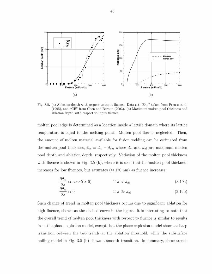
45

Fluence [mJ/cm^2]

Ablationdepth[nm]

0 100 200 300 4000

10

20

30

FEMExpCB

(a)

Fluence [mJ/cm^2]

Thickness[nm]

0 200 400 600 8000

50

100

150

200

AblationMolten pool

(b)

Fig. 3.5. (a) Ablation depth with respect to input fluence. Data set “Exp” taken from Preuss et al.(1995), and “CB” from Chen and Beraun (2003). (b) Maximum molten pool thickness andablation depth with respect to input fluence

molten pool edge is determined as a location inside a lattice domain where its lattice

temperature is equal to the melting point. Molten pool flow is neglected. Then,

the amount of molten material available for fusion welding can be estimated from

the molten pool thickness, θm ≡ dm − dab, where dm and dab are maximum molten

pool depth and ablation depth, respectively. Variation of the molten pool thickness

with fluence is shown in Fig. 3.5 (b), where it is seen that the molten pool thickness

increases for low fluences, but saturates (≈ 170 nm) as fluence increases:

∂θm

∂J≈ const(> 0) if J < Jab (3.19a)

∂θm

∂J≈ 0 if J - Jab (3.19b)

Such change of trend in molten pool thickness occurs due to significant ablation for

high fluence, shown as the dashed curve in the figure. It is interesting to note that

the overall trend of molten pool thickness with respect to fluence is similar to results

from the phase explosion model, except that the phase explosion model shows a sharp

transition between the two trends at the ablation threshold, while the subsurface

boiling model in Fig. 3.5 (b) shows a smooth transition. In summary, these trends

46

of molten pool evolution indicate that only a limited amount of molten pool can be

obtained from a single ultrashort laser pulse, regardless of input fluence, which is a

disadvantage for welding. But, it should also be noticed that the limited molten pool

evolution can be considered as favorable for precise material removal.

The limitation on molten pool development may still exist for multiple pulses if

repetition rates are low, since the temperature then cools down to its initial temper-

ature between pulses. To study this case, two consecutive pulses with high repetition

rates in the range of 0.1 ∼ 10 GHz are considered. Pulse duration of 500 fs and low

input fluence of 100 mJ/cm2 are selected as laser parameters. A low fluence is used to

minimize the ablation effect. A heat source term for two pulses (S2), which replaces

the heat source (S) of Eq. (3.1) in this case study, is defined as follows:

S2(x, t) =

S(x, t) if t < 1/f

S(x, t) + S(x, t − 1/f) if t ≥ 1/f

where f is the pulse repetition rate, and S(x, t) is defined in Eq. (3.17). It is assumed

that there is no surface condition change of the target material after the first irradia-

tion, i.e., the same reflectivity is used for both pulses. The calculation was conducted

over a long enough period to account for heating and cooling of the material due to

the two pulses.

Molten pool evolution histories for select repetition rates are shown in Fig. 3.6

(a). It can be observed from the figure that repetition rates higher than 2.5 GHz will

enable continuous existence of molten pool inside the material. To demonstrate the

effect of multiple pulses, the maximum relative molten (θm,2/1) and ablation (θab,2/1)

thicknesses are defined as θm,2/1 ≡ θm,2/θm,1 and θab,2/1 ≡ θab,2/θab,1, respectively,

where θm,1 and θm,2 are maximum molten pool thickness after the first and second

pulse, and θab,1 and θab,2 are ablation thickness after the first and second pulse, re-

spectively. Those are plotted in Fig. 3.6 (b). The figure shows that the molten pool

thickness after the second pulse is generally larger than the one after the first pulse.

It can also be observed that the molten depth saturates as repetition rates increase,

due to increased ablation for the high repetition rates. It is interesting to note that

47

Time [ps]

Moltenpooldepth[nm]

100 101 102 103 1040

50

100

150

200

250

0.2GHz

1GHz

2.5GHz

8GHz

J=100mJ/cm^2

(a)

Repetition rates [GHz]

Max.Relativemoltenpoolthickness

Relativeablationthickness

10-1 100 1011

1.5

2

2.5

3

0

50

100

150

200

⇒

⇒

J=100mJ/cm^2

(b)

Fig. 3.6. (a) Lattice temperature histories at the top surface for select pulse repetition rates. (b)Maximum relative molten pool and ablation thicknesses with respect to repetition rates.In the figure, pulse duration is 500 fs.

two pulses at high repetition rates result in more than two and a half times deeper

molten pool thickness. Thus, repetition rates on the order of 10 GHz are expected to

enable more molten pool in the target material, which may provide favorable condi-

tions for laser micro welding with UFL. However the ablation rate also increases with

repetition rate. On the other hand, the high repetition rates may not be appropriate

for material removal, due to the increased molten pool generation.

3.4.2 Feasibility of LMW with UFL - pulse duration

The second case study involves the feasibility of laser microwelding for different

pulse durations. Pulse durations in the range from fs to sub-ns are considered with the

TTM implementation in ABAQUS. The validity of the TTM implementation for dif-

ferent pulse durations is examined by comparison with experimental results from the

literature. The effect of pulse duration on molten pool generation is then investigated

numerically. Finally, local disequilibrium for different pulse durations is investigated,

which is closely related to the validity of the conventional heat conduction model with

respect to pulse duration.

48

Pulse width [ps]

Ablationthresholdfluence[J/cm^2]

10-1 100 101 102 1030

2

4

6

8

FEMExp

domain thickness = 1.0 micronablation criterion:ablation depth > 0.1nm

(a)

Time [ps]

Ablationdepth[nm]

100 101 102 1030

10

20

30

40J=4J/cm^2

tp=100fstp=1ps

tp=10ps

tp=100ps

(b)

Fig. 3.7. (a) Ablation threshold fluence with respect to pulse duration. Experimental data set “Exp”taken from Furusawa et al. (1999). (b) Ablation histories at the top surface for select pulsedurations with J = 4 J/cm2.

The material to be processed is again selected as gold. Boundary conditions,

initial conditions, the material model and the related constants are identical to the

previous case study except for the heat source reflectivity, due to the change of laser

wavelength to λ = 800 nm, from 248 nm of the previous case study. The corresponding

reflectivity is listed in Table 3.3. The pulse duration range of interest is 100 fs ≤ tp ≤

100 ps.

The ablation threshold fluence is defined as the fluence that results in an ablation

depth of 0.1 nm in this study. The threshold fluences are obtained from interpolative

calculations for a given pulse duration while varying fluences to obtain the abla-

tion depth of 0.1 nm. The numerical results of ablation threshold fluence obtained

from ABAQUS and experimental results of Furusawa et al. (1999) are compared in

Fig. 3.7 (a). Both results show overall increasing trends of ablation threshold fluence

as pulse duration increases, which demonstrate validity of the model for qualitative

estimations. Corresponding ablation histories for different pulse durations with J = 4

J/cm2 are shown in Fig. 3.7 (b). The figure shows that shorter pulse duration results

in deeper ablation depth for a given fluence. This demonstrates that shorter pulse

49

Fluence [J/cm^2]

Max.moltenpoolthickness[nm]

0 2 4 6 80

100

200

300

400

500

tp=100fs

tp=1ps

tp=10ps

tp=100ps

(a)

Pulse width [ps]

Moltenpoolthickness[nm]

Ablationdepth[nm]

10-1 100 101 1020

100

200

300

400

0

10

20

30

40

J=2.0,Pool

J=4.0, Pool

J=4.0,Ablation

J=2.0,Ablation

J in [J/cm^2]

(b)

Fig. 3.8. (a) Maximum molten pool thickness with respect to input fluence for select pulse durations.(b) Corresponding molten pool thickness and ablation depth with respect to pulse duration

durations are favorable for material removal.

Next, the effect of pulse duration on molten pool thickness is examined by tracking

the molten pool edges for select pulse durations, as shown in Fig. 3.8. In the figure,

all the pulse durations show similar molten pool generation trends for low fluence of

J < Jab, i.e., Eq. (3.19a) is still valid for long pulse durations. However, the long

pulse duration of 100 ps in the figure shows a significantly different trend from the

short pulse durations, Eq. (3.19b), in which the molten pool thickness increases as

fluence increases. Thus, Eq. (3.19b) for J - Jab should be revised for pulse durations

as follows:

∂θm

∂J≈ 0 if tp ≤ 10 ps (3.20a)

∂θm

∂J- 0 if tp - 10 ps (3.20b)

It is interesting to note from Fig. 3.7 (b) and Fig. 3.8, especially for the higher fluence

of 4 J/cm2, that the molten pool thickness increases but ablation depth decreases,

as pulse duration increases. Thus, it can be deduced that ablation and molten pool

dominant pulse duration ranges are mutually exclusive. In addition to the energy

50

Depth [nm]

Tl[X1000

K]

0 200 400 600 800 1000

2

4

6

810

J=8J/cm^2, tp=1pst=5ps

t=0.1ns0.3ns0.5ns0.7ns0.9ns

(a)

Depth [nm]

Tl[X1000

K]

0 200 400 600 800 1000

2

4

6

810

t=210ps

t=500pst=1ns

t=2nst=3ns

J=8J/cm^2, tp=100ps

(b)

Fig. 3.9. Lattice temperature distributions at select times with fluence of 8 J/cm2 for pulse durationof (a) 1 ps, and (b) 100 ps; Horizontal dot-dashed line in both figures represents the meltingpoint.

removal effect of ablation, the exclusiveness may also be related to the dependence of

thermal penetration depth (δth) on the time scale of energy supply, i.e. δth =√κ · tp,

where κ and tp are the thermal diffusivity and laser pulse duration, respectively.

These imply that 1) longer pulse durations provide more favorable conditions for

laser microwelding of micrometer-scaled objects than shorter pulse durations, 2) the

input fluence should be stable for laser microwelding with longer pulse durations to

avoid total melting of the objects.

The lattice temperature distributions at select times for different pulse durations,

tp = 1 and 100 ps, are shown in Fig. 3.9. The figures indicate that temperatures

do not return to their initial value of T0 at the final steady state, but converge to a

final equilibrium temperature higher than T0, mainly due to the adiabatic boundary

condition, Eq. (3.18), for the limited domain size. In other words, the boundary

condition neglects energy loss across the boundary, which may not represent the real

situation correctly, especially for an energy input and response over a long time in

small domain. However, the boundary condition is adequate for investigating the

thermal behavior of a material in the initial stages of the response. Those show that

51

Pulse width [ps]

Te,max-Tl,max[X1000K]

t(Te,max)-t(Tl,max)/tp

10-1 100 101 1020

20

40

60

10-1

100

101

102

2J/cm^24J/cm^2

⇒

⇒

(a)

Time [ps]

Te,Tl[X1000

K]

0 5000 10000 150000

1

2

3

TTMOTM

J=8J/cm^2, tp=5ns

x=0

x=Lx

(b)

Fig. 3.10. (a) Difference between maximum electron and lattice temperature for select fluences withrespect to pulse duration, and corresponding relative time delay between electron andlattice maximum temperatures; in the figure, “Te,max” and “Tl,max” represent Te,max

and Tl,max, respectively. (b) Comparison of temperature histories at the top and bottomsurface evaluated from the TTM and conventional heat conduction model (denoted as“OTM” in the legend) for tp = 5 ns, J = 8 J/cm2; in the figure, Te and Tl represent Te

and Tl, respectively.

longer pulse durations result in higher temperatures in the overall domain and at the

other end of the domain as time proceeds, i.e. deeper thermal penetration.

It is well known that the pulse duration is closely related to local disequilibrium

between electrons and the lattice of a metal. To quantify the disequilibrium, the

difference between electron and lattice temperatures, ∆Tmax, and relative time delay

between temperatures, ∆t(Tmax), are defined as:

∆Tmax ≡ Te,max − Tl,max

∆t(Tmax) ≡(

t(Tl,max) − t(Te,max))

/tp

where Te,max and Tl,max are maximum electron and lattice temperatures, respectively,

for given laser input and t(Te,max) and t(Tl,max) are times when electron and lattice

temperatures reach their respective peaks. The temperature deviation and the relative

time delay are shown in Fig. 3.10 (a), which shows that both temperature deviation

and relative time delay decrease as pulse duration increases. More specifically, the

52

relative time delay shows a simple dependency on fluence, with higher fluence resulting

in lower relative time delay. However, the temperature deviation shows a different

trend from the time delay, i.e., higher fluence results in higher temperature deviation

for shorter pulse durations than lower fluence, but lower deviation for longer pulse

durations. Thus, the disequilibrium is negligible for laser pulse with longer pulse

durations. To demonstrate this, when the energy interaction term, E, is eliminated

from Eq. (3.1) with T = Te = Tl, we have

(

Ce + Cl

)

·∂T

∂t= $∇ · $qe + S

This is identical to the conventional heat conduction equation. Both the conventional

heat conduction model and the TTM give similar results, Fig. 3.10 (b), for long pulse

duration (tp ≥ 5 ns) and high fluence (J = 8 J/cm2). Thus, the conventional heat

conduction model is appropriate for pulse durations of the order of ns.

3.4.3 Feasibility of LMW with UFL - focal radius

The last case study is the effect of focal radius on feasibility of laser microwelding,

which is analyzed using an axisymmetric 3D domain in ABAQUS.

The geometry is illustrated in Fig. 3.11 (a), with radius (R) and thickness (Z)

of 3.0 and 0.5 µm, respectively. The domain is constructed using finite element

“CAX4T”, which replaces “CPS4T” of the 1D linear configuration.Gold is the pro-

cessed material, as in the previous case studies. An axisymmetric heat source is

defined for Gaussian and exponentially decaying distributions in the radial (r) and

depth (z) coordinates, respectively, and Gaussian temporal profile as:

S(x, t) ≡ J · (1 − R) ·√

b/π

tp · δs· exp

[

−(

r

rf

)2

−(

z

δs

)

− b ·(

t − 2tptp

)2]

Initial (IC) and boundary (BC) conditions are also extended for axisymmetric 3D

53

(a)

Radius [nm]

Depth[nm]

0 500 1000 1500

50

40

30

20

10

0

rf=0.5umrf=1.0um

tp=500fsJ=800mJ/cm^2

J=200

(b)

Fig. 3.11. (a) Axisymmetric 3D dual domain configuration. (b) Ablated top surface (z = 0) profilefor select focal radii and fluences. Note that unit length scales are different for depth andradius coordinates.

geometry as follows:

IC: Te(r, z, 0) = Tl(r, z, 0) = T0, qe(r, z, 0) = 0

BC: qe(r, 0, t) = qe(r, Z, t) = 0, qe(0, z, t) = qe(R, z, t) = 0

For laser parameters, wavelength λ = 248 nm, focal radii rf = 0.5 and 1.0 µm,

pulse duration tp = 0.5 and 500 ps, and fluence J = 200, 400 and 800 mJ/cm2 are

considered.

The ablated profiles of the top surface (z = 0) for select fluences and focal radii

at tp = 0.5 ps are shown in Fig. 3.11 (b). As the figure indicates, different focal radii

with the same fluence result in the same maximum depth at the center (r = 0), and

smaller focal radius with the same energy per pulse results in deeper ablation depth,

as can be seen from comparison between the cases of J = 200 with rf = 1.0 µm and

J = 800 with rf = 0.5 µm. Thus for a given energy input, a smaller focal radius with

higher fluence may be more efficient for precise material removal, and that fluence is

one of the key parameters that determines ablation depth.

Molten pool edges at select times for rf = 0.5 µm, J = 800 mJ/cm2 and tp =

0.5 ps are shown in Fig. 3.12 (a). It is evident that the molten pool is relatively

54

r [nm]

z[nm]

0 250 500 750 1000500

250

0

t=20psmax. pool radius

t=200psmax. pool depth

t=400ps

t=700ps

J=800mJ/cm^2, rf=0.5um

Ablated surfaces for t >= 20ps

(a)

r [nm]

z[nm]

0 250 500 750 1000500

250

0

t=1.2ns, dashed curvemax. pool radius

t=1.3ns, solid curvemax. pool depth

t=1.5ns

t=1.7ns

Top surface(No ablation)

J=400mJ/cm^2, rf=0.5umtp=500ps

(b)

r [nm]

z[nm]

0 250 500 750 1000500

250

0

J=800,rf=1.0@ t=900ps

J=800,rf=0.5@ t=300ps

J in [mJ/cm^2], rf in [um]

J=200,rf=1.0@ t=200ps

J=200,rf=0.5@ t=100ps

Ablated surfaces forJ=800, rf=0.5

J=800, rf=1.0

(c)

r [nm]

z[nm]

0 250 500 750 1000500

250

0

tp=0.5ps,rf=0.5um@t=0.2ns

tp=0.5ps,rf=1.0um@t=0.5ns

tp=500ps,rf=0.5um@t=1.3ns

tp=500ps,rf=1.0um@t=2.0ns

Top surfaces fortp=500ps (no ablation)tp=0.5ps, rf=0.5umtp=0.5ps, rf=1.0um

J=400mJ/cm^2

(d)

Fig. 3.12. Molten pool edge and top surface profile developed by a beam radius of rf = 0.5 µm atselect times for (a) J = 800 mJ/cm2 and tp = 0.5 ps, and for (b) J = 400 mJ/cm2 andtp = 500 ps; Comparison of molten pool edges developed by select beam focal radii atthe times of maximum depths for (c) select fluences and tp = 0.5 ps, and (d) select pulsedurations and J = 400 mJ/cm2

55

shallow for short pulse durations. It takes about 10 ps for the molten pool to reach

its maximum size in the radial direction, but of the order of 100 ps for the depth. On

the other hand, as can be seen from Fig. 3.12 (b) for a longer pulse duration tp = 500

ps, the time scale for the molten pool development in the depth and radial directions

are similar, i.e., maximum pool diameter at t = 1.2 ns and maximum pool depth at

t = 1.3 ns. Molten pool edges of select fluences and focal radii for tp = 0.5 ps at

the time of maximum pool depth are shown in Fig. 3.12 (c). It is interesting to note

from the figure that different maximum molten pool depths are obtained for the same

fluence when the focal radius is changed, i.e., a deeper molten pool can be obtained

for a larger focal radius with the same fluence, which corresponds to a higher energy

per pulse. This trend is different from the one observed for the ablation depth and

input fluence. Also, a higher fluence results in a deeper molten pool depth for the

same energy per pulse, as can be seen by comparing the cases of J = 200 with rf =

1.0 µm and J = 800 with rf = 0.5µm. Thus, higher energy per pulse and fluence may

provide more favorable conditions for laser microwelding with UFL. However, from

the viewpoint of precise material removal, smaller focal radius and energy per pulse

might be preferable, as it would result in better quality with reduced molten material.

It can be seen from Fig. 3.12 (d) that longer pulse durations can produce similar or

deeper molten pools for the same fluence. As focal radius increases, shorter pulse

durations result in significant increase in molten radius, while longer pulse durations

increase the depth. Thus longer pulse durations enable more favorable conditions for

laser microwelding for a given fluence or energy per pulse.

3.5 Conclusions

The feasibility of laser microwelding using ultrafast lasers is numerically investi-

gated for select parameters of pulse repetition rate, pulse duration, and focal radius,

by implementing the two-temperature model in ABAQUS. A material model is con-

structed using models derived from physics and the subsurface boiling model for

ablation. The validity of the model is investigated by comparison with experimental

56

results from the literature.

For the conditions examined, the results indicate that laser microwelding is feasible

for 1) low fluence ultrashort pulses with high repetition rates of the order of 1 ∼ 10

GHz, 2) longer pulses from a stable laser generator with high fluence capability, or 2)

larger focal radius for a given fluence i.e., high energy per pulse and fluence. On the

other hand, the results indicate that lower repetition rate, shorter pulse duration, and

smaller focal radius for a given fluence provide favorable conditions for precise material

removal such as laser cutting or drilling, as those conditions maximize ablation, and

minimize molten pool generation.

Chapter IV

Experimental investigation of laser shock peening usingfemtosecond laser pulses

4.1 Introduction

Surface treatment has been widely used to improve wear and fatigue resistance in

several applications (Kalpakjian and Schmid, 2001). Laser shock peening is known

to be superior to conventional shot peening for such surface treatment since it results

in deeper compressive residual stresses and smoother processed surface, and is also

more suited for localized processing (Montross et al., 2002).

Following early studies on momentum transfer (Gregg and Thomas, 1966) and

stress waves generation inside a target metal (Anderholm, 1970) due to laser pulses,

laser shock peening (LSP) for surface treatment has been intensively investigated for

various materials, including steel (Peyre et al., 2000; Yilbas et al., 2003; Yakimets

et al., 2004; Aldajah et al., 2005; Farrahi and Ghadbeigi, 2006), aluminum (Fairand

et al., 1972; Peyre et al., 1996; Hong and Chengye, 1998; Rubio-Gonzalez et al.,

2004; Tan et al., 2004) and nickel alloy, molybdenum and copper (Forget et al., 1990;

Hammersley et al., 2000; Kaspar et al., 2000; Zhang et al., 2004). It has also been

successfully applied to improve fatigue life of automotive ring and pinion gears and

aircraft engine turbine blades (See et al., 2002).

A high power Q-switched Nd:YAG laser with pulse duration of the order of 1

∼ 100 ns is frequently used for laser shock peening, and the specimen is usually

prepared with a thermo-protective absorbing coating with a transparent confining

layer on top, to maximize the effect of the process (Fabbro et al., 1998; Montross

et al., 2002). Despite significant improvements over the years, Fabbro et al. (1998)

57

58

indicated the potential for improving the process by adopting extremely short laser

pulses to achieve higher pressure, and thus deeper processed layers.

Ultrashort laser pulses, or ultrafast lasers (UFL), of sub-picoseconds pulse du-

ration have been investigated experimentally, primarily for material removal (Nolte

et al., 1997; Dumitru et al., 2002; Pronko et al., 1995; Zhu et al., 1999). Liu et al.

(1997) discuss laser-matter interaction involving femtosecond laser pulses in detail.

Femtosecond laser pulses are expected to be a good tool not only for material

removal, but also for shock generation inside a metal, due to its extremely short pulse

duration (Fabbro et al., 1998). This can be inferred from experimental demonstration

of acoustic signal generation using short laser pulse durations between 100 fs and 150

ps (Dehoux et al., 2006).

There have been few investigations on laser shock peening using short pulses of

the order of picosecond or femtosecond duration. Banas et al. (1990) conducted an

experiment using a pulse duration of 150 ps for laser shock peening of an uncoated

steel in water confined configuration, and Chu et al. (1999) used a pulse duration of

600 ps for low carbon steel in vacuum. However, Kaspar and Luft (2001) indicated

in their experiment using a pulse duration of 210 fs for molybdenum without a top

coating that the shock affected depth for the femtosecond laser pulses is too shallow to

make femtosecond pulses interesting for laser shock peening application, even though

the femtosecond laser pulses deliver higher peak pressure than longer pulse duration

lasers. They also indicated that optical breakdown of the transparent confining layer,

water, may limit the possibility of valid laser shock peening with femtosecond laser

pulses. This is discussed by Vogel et al. (2005) in greater detail. Thus, it can be sum-

marized that the process of laser shock peening using sub-picosecond pulse duration

needs further investigation.

In this study, the feasibility of laser shock peening of top coated steel in water

confined configuration using ultrafast laser pulses is experimentally investigated. Op-

tical breakdown of the transparent confining layer and selection of the top coating

material are carefully considered to enhance the prospect of laser shock peening using

ultrafast laser pulses.

59

Fig. 4.1. A water confined configuration for laser shock peening

4.2 Background

The laser shock peening process is illustrated schematically in Fig. 4.1. As sum-

marized by Fabbro et al. (1998) and Montross et al. (2002), a confining layer and

top coating are used to maximize the laser induced pressure on the top surface of the

target material.

One of the potential advantages of using UFL for LSP over long pulse duration

laser is their ability to minimize thermal penetration depth (δs), which is related to

the pulse duration (tp) and thermal diffusivity (α) by δs ∝√α · tp (Mills, 1992; Liu

et al., 1997). In addition, a shorter pulse duration is expected to increase pressure

(P ) induced by the laser (Fabbro et al., 1998; Dehoux et al., 2006). Fabbro et al.

(1998) presented a relation between pressure (P ) induced by the laser and the depth

(Lp) of the plastically deformed region, which can be expressed as

Lp ∝ tp · P and P ∝√

I0

where tp, I0 and P are the pulse duration, beam intensity and pressure generated

by the laser input, respectively. This indicates that a shorter pulse duration may

result in a relatively thin shock peened layer. Hence, further investigation is needed

to determine whether the laser induced pressure increment can compensate for the

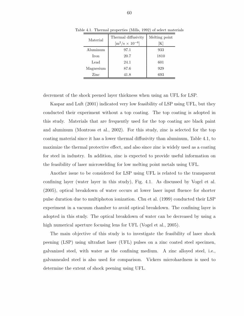
60

Table 4.1. Thermal properties (Mills, 1992) of select materials

MaterialThermal diffusivity Melting point

[m2/s × 10−6] [K]

Aluminum 97.1 933

Iron 20.7 1810

Lead 24.1 601

Magnesium 87.6 929

Zinc 41.8 693

decrement of the shock peened layer thickness when using an UFL for LSP.

Kaspar and Luft (2001) indicated very low feasibility of LSP using UFL, but they

conducted their experiment without a top coating. The top coating is adopted in

this study. Materials that are frequently used for the top coating are black paint

and aluminum (Montross et al., 2002). For this study, zinc is selected for the top

coating material since it has a lower thermal diffusivity than aluminum, Table 4.1, to

maximize the thermal protective effect, and also since zinc is widely used as a coating

for steel in industry. In addition, zinc is expected to provide useful information on

the feasibility of laser microwelding for low melting point metals using UFL.

Another issue to be considered for LSP using UFL is related to the transparent

confining layer (water layer in this study), Fig. 4.1. As discussed by Vogel et al.

(2005), optical breakdown of water occurs at lower laser input fluence for shorter

pulse duration due to multiphoton ionization. Chu et al. (1999) conducted their LSP

experiment in a vacuum chamber to avoid optical breakdown. The confining layer is

adopted in this study. The optical breakdown of water can be decreased by using a

high numerical aperture focusing lens for UFL (Vogel et al., 2005).

The main objective of this study is to investigate the feasibility of laser shock

peening (LSP) using ultrafast laser (UFL) pulses on a zinc coated steel specimen,

galvanized steel, with water as the confining medium. A zinc alloyed steel, i.e.,

galvannealed steel is also used for comparison. Vickers microhardness is used to

determine the extent of shock peening using UFL.

61

(a) (b)

Fig. 4.2. (a) Overall layout of experimental set-up (b) A focused UFL forming a visible spot in air

4.3 Experiment

The overall experimental set-up is shown in Fig. 4.2 (a). A Clark-MXR CPA-2001

laser was used in this experiment (λ = 775 nm, 0.8 mJ @ 1 kHz, tp ≈ 200 fs). The

beam is guided by mirrors to an aspheric focusing lens of high numerical aperture,

NA ≈ 0.5. The lens is selected 1) to obtain a small focal diameter to minimize

spherical aberration (Hecht, 2002), resulting in high input fluence (J) for a given

laser beam power with better beam quality on the focal plane, and 2) to minimize

optical breakdown of a confining water medium for a given laser fluence (Vogel et al.,

2005). The lens is mounted on an one-axis linear stage to align the focal plane with

the specimen top surface by observing a visible spot formed by the focused UFL,

Fig. 4.2 (b).

Neutral density filters of optical density (OD) labeled as 0.5, 1.0 and 2.0 are used

to control the laser power (and fluence). The actual OD values of the filters were

measured by comparing the laser beam power obtained with or without the filters,

and the values are used to evaluate corresponding fluences (J) with the filter using

the relationship J = 10−OD · J0, where J0 is the fluence without the filters. The

laser fluence J0 was estimated from measured laser beam powers and a focal diameter

estimated as follows: Actual average power of the laser beam (P ) was measured using

a power meter. The average power obtained for several measurements was 643.7 ±

62

(a)

(b)

Fig. 4.3. (a) Two examples of microscope photos for single line scanning on the top surface ofgalvanized steel specimen. (b) Scanning pattern on the top surface of a specimen.

5.8 mW. The width of the single line scan was measured from microscope photos,

and taken as the focal diameter (d), Fig. 4.3 (a). The focal diameter was estimated

to be 122.8 ± 15.7 µm. Thus, the input fluence J0 is obtained as 5.43 J/cm2, from

J0 = P/(0.25πd2 · φ), where φ is the repetition rate of the laser pulse. At this

point, it should be noted that the width of the scanned line in the figure does not

exactly represent the focal diameter, but is strongly related to the diameter and input

fluence. Thus the fluence value is not absolute, but rather a relative measurement.

Moreover, the focal diameter is strongly dependent on the distance between the target

top surface and focusing lens, especially for high NA focusing lens. This may increase

uncertainty in fluence values in this experiment. These values were used in estimating

the fluence and the results are summarized in Table 4.2. It should be noted that the

fluence estimation does not consider any uncertainty for the beam delivery system

and the confining configuration for laser shock peening, for example, reflection loss of

mirrors and absorption of the confining water.

The water layer thickness was 2 mm, and was controlled using an injection needle.

The specimen was mounted in the water container, which was installed on a two-axes

computer-controlled linear stage. The specimens were processed on the top surface

with each scan line being 4 mm in length, and spaced apart by 10 µm pitch, Fig. 4.3

(b).

63

Table 4.2. Labeled and measured optical densities (OD) of neutral density filters and correspondingfluences calculated from J = 10−OD · J0, where J0 = 5.43 J/cm2

OD, labeled OD, measured Fluence [J/cm2]

0.5 0.50 1.73

1.0 0.99 0.21

2.0 1.78 0.09

Table 4.3. Chemical composition (wt%) of an AKDQ steel (Zhang and Senkara, 2006)

C Mn P S Si Cu Ni Cr Mo Sn Al Ti

0.035 0.210 0.006 0.011 0.007 0.020 0.009 0.033 0.006 0.004 0.037 0.001

The specimens were as-received 1 mm thick galvanized and galvannealed AKDQ

steel sheets, Table 4.3 (Zhang and Senkara, 2006). The galvanized steel was the main

material for the LSP experiment, considering the zinc coating of the steel as the top

metallic ablative coating for laser shock peening. The thickness of the zinc coating

on galvanized steel was measured from a cross-section, Fig. 4.4, of the specimen and

ranged from 16.0 to 39.3 µm, with an average value of 26.9 µm. The galvannealed

steel was used for a comparison study on the effect of the metallic coating.

For the galvanized steel, a full factorial experimental design was used with two

factors of laser input fluence (J) and feed rate (f), with four levels for the input

fluence (three fluences with, and one without the filters) and two levels for feed rate,

(a)

(b)

Fig. 4.4. Sections of (a) galvanized, and (b) galvannealed steel specimens. Specimens were sectioned,cold mounted, polished and etched using 0.5% nitol (Vander Voort, 2004).

64

500 and 1000 µm/s. A slow feed rate of 50 µm/s was separately investigated. For the

galvannealed steel, a fixed feed rate of 500 µm/s was used. After the experiments,

the top surface Vickers microhardness values of the specimen were measured using

Buehler’s Micromet II. The microhardness values for galvanized and galvannealed

steel specimens on the top surfaces before the experiment were found to be 69.5 ±

4.0 and 121.5 ± 2.4 Hv, respectively. The microhardness of base low carbon steel was

found to be 97.6 ± 1.8 Hv. The uncertainty of measurement was determined with

a 99% confidence level. After processing, the microhardness of each specimen was

measured 10 times. The microscope was used for visual inspection of the top surface,

and for estimating the maximum depth of the processed region using a 40X objective

lens which has a shallow depth of focus, thus providing high spatial resolution.

4.4 Results and discussion

The effect of input fluence and feed rate on microhardness of galvanized steel spec-

imens is examined first, Fig. 4.5 (a). For f = 500 µm/s, the microhardness is observed

to increase abruptly between 0.09 and 0.21 J/cm2 fluence, and level off at 106.7 ±

8.2 Hv, as fluence increases above 0.21 J/cm2. The level off value was statistically

determined from mean difference tests with 1% significance level (Montgomery, 1991)

on microhardness values for J = 0.21, 1.73 and 5.43 J/cm2. For f = 1000 µm/s, the

level off is observed at 95.5 ± 6.0 Hv, but only for J = 1.73 and 5.43 J/cm2. However,

it is not clear whether f = 500 µm/s results in higher microhardness than f = 1000

µm/s since those level off values are within the uncertainty range of each other. The

mean difference test also indicates that there is no significant difference between the

level off hardness for f = 500 and 1000 µm/s. The uncertainty is mainly due to the

surface roughness of the LSP regions, and different hardness values for the various

iron-zinc intermetallic phases that may form (Korb and Olson, 1987). However, it

is interesting to note that the level off value for f = 1000 µm/s is very close to the

original value of the base steel, 97.6 ± 1.8 Hv. Considering the fluence values of J2 =

0.21 and J3 = 1.73 J/cm2 for galvanized steel, Fig. 4.10 (a), and the observation that

65

Fluence [J/cm^2]

Microhardness[Hv]

10-2 10-1 100 10160

80

100

120

140

feed = 500 um/sfeed = 1000 um/s

(a)

Fluence [J/cm^2]

Maximum

depthofprocessedregion

[um]

10-2 10-1 100 1010

20

40

60

feed = 500 um/sfeed = 1000 um/s

(b)

Fig. 4.5. Experimental data comparison of galvanized steel specimens for select feed rates, f = 500and 1000 µm/s, with respect to input fluence: (a) Microhardness. (b) Maximum depth ofthe processed region. In the figure, “um” represents µm.

the microhardness levels off for J ≥ 0.21 J/cm2, Fig. 4.5 (a), it can be deduced that

the bright top surface is due to a thin zinc layer until complete zinc removal occurs

when J ≥ 5.43 J/cm2. Material removal occurs mainly for zinc when 0.09 ≤ J <

1.73 J/cm2; then for steel when J ≥ 1.73 J/cm2. Thus the microhardness increment

is mainly due to removal of the soft top coating.

Figure 4.5 (b) shows the corresponding maximum depth of the processed region.

The maximum depth is observed to be more than the zinc layer thickness (26.9 µm

average) for high fluence when f = 500 µm/s. It is interesting to note from the figure

that the maximum depth for galvanized steel, which has zinc coating on top of steel,

follows the trend of two logarithmic dependency with respect to the input fluence,

as discussed by Nolte et al. (1997). The microhardness for f = 50 µm/s could not

be measured for high fluence due to the formation of a severe groove, Fig. 4.6, but

was measured for low fluence. However, the microhardness for f = 50 µm/s with

the low fluence was not significantly different from the value for f = 500 µm/s. It

should be noted that debris generation was observed for f = 50 µm/s, Fig. 4.7 (b),

which became more severe as feed rate decreased and fluence increased. The debris

66

Fig. 4.6. Section of galvanized steel specimen after LSP with J = 5.43 J/cm2 for feed rate of (a)500 µm/s and (b) 50 µm/s

(a) (b)

Fig. 4.7. Debris generated during galvanized steel experiment: (a) Before and (b) after the experi-ment

generation is one possible reason for the microhardness leveling off at the high fluence.

To minimize the debris interference, the water in the container was replaced after each

run. But this did not completely eliminate debris interference during an experimental

run. Such debris generation, however, was not observed during experiments with

the galvannealed steel specimen. Another possible reason for the level off is optical

breakdown of water. Vogel et al. (2005) state that optical breakdown of water occurs

for fluence higher than 5.6 J/cm2 by femtosecond laser pulses (pulse duration = 100 fs,

wavelength = 800 nm) focused using a lens of NA = 0.65. The level off was observed

for fluence higher than 0.21 J/cm2 with NA ≈ 0.5 in this study. Even though the level

67

Table 4.4. ANOVA table of data for galvanized steel. In the table, “DoF” stands for degree offreedom. “Fcrit” is the critical F ratio for a given degree of freedom. Levels for thefactors J and f are 0.09, 0.21, 1.73 and 5.43 J/cm2, and 500 and 1000 µm/s, respectively.

Source of variation DoF Sum of Squares Mean Squares F Fcrit p-value

Fluence, J 3 150181 50060 215.3 3.8 p 0 1.0 × 10−13

Feed rate, f 1 10833 10833 46.6 6.7 1.6 × 10−11

Interaction, J × f 3 14406 4802 20.7 3.8 5.8 × 10−13

Error 934 217139 232 – – –

Total 941 392558 – – – –

off fluence is lower than the threshold fluence, the possibility of optical breakdown

for J ≥ 0.21 J/cm2 cannot be completely ruled out due to the lower NA used in this

study, and uncertainty of the focal diameter estimation, i.e., the focal diameter from

line scans, Fig 4.3 (b), might be an overestimation. The optical breakdown of water

was not experimentally investigated in this study. However, it is interesting to note

that the microhardness did not change drastically for high fluence, Fig. 4.5 (a), while

material removal occurred significantly for the fluence, Fig. 4.5 (b). This indicates

that the femtosecond laser is a good tool for material removal for the conditions used

in this experiment.

Table 4.4 summarizes ANOVA results (Montgomery, 1991) of microhardness val-

ues obtained from galvanized steel experiments with factors J (four levels - 0.09, 0.21,

1.73 and 5.43 J/cm2) and f (two levels - 500 and 1000 µm/s). For the levels studied,

the large F ratio for J in Table 4.4 indicates that the fluence has the dominant effect

on microhardness. The feed rate (f) and interaction effects on the microhardness is

relatively small. The small effect of feed rate may be due to the fact that the number

of shots is related to both feed rate and scanning line distance, 10 µm, Fig. 4.3 (b),

which was kept constant in this experiment. It should also be noted that Duncan’s

post test (Montgomery, 1991) on microhardness indicates that all the fluences, ex-

cept the lowest ones, result in the same microhardness, which confirms the previous

observation from mean difference tests, and from Fig. 4.5 (a).

Next, the effect of top coating on microhardness is examined by comparing the

hardness of processed galvanized and galvannealed steel specimen, Fig. 4.8 (a). In

68

Fluence [J/cm^2]

Microhardness[Hv]

10-2 10-1 100 10160

80

100

120

140

galvanized steelgalvanealed steel

(a)

Fluence [J/cm^2]

Maximum

depthofprocessedregion

[um]

10-2 10-1 100 1010

20

40

60

galvanized steelgalvanealed steel

(b)

Fig. 4.8. Experimental data comparison of galvanized and galvannealed steel specimens for feed ratef = 500 µm/s, with respect to input fluence: (a) Microhardness. (b) Maximum depth ofthe processed region. In the figure, “um” represents µm.

the figure, the galvanized steel results for f = 500 µm/s of Fig. 4.5 is re-plotted

for comparison. The microhardness of galvannealed steel is observed to decrease

slightly as fluence increases, which is a different behavior from galvanized steel. It

also shows less significant dependence of the hardness on fluence than galvanized steel.

Mean difference tests with 1% significance level was conducted on microhardness

values for J = 1.73 and 5.43 J/cm2 of galvannealed steel specimen, and resulted

in the same values of 97.2 ± 6.1 Hv. The test was also conduced for J = 1.73

J/cm2 on both materials, and indicated that there is no difference in the values.

But the test for J = 5.43 J/cm2 of both materials resulted in higher microhardness

for galvanized steel than for galvannealed steel. However, from the uncertainties in

microhardness values, it is difficult to conclude whether the results are significantly

different. The maximum depth of processed region for galvannealed steel also shows

the two logarithmic dependency (Nolte et al., 1997), Fig. 4.8 (b), but a shallower

depth than galvanized steel. The depth difference for the two materials is due to the

fact that one has zinc as an alloy, while the other has it as a coating, resulting in

different absorption characteristics.

69

(a)

(b)

Fig. 4.9. Two possibilities on a relation between UFL input fluence and hardness at top surface ofbase material: (a) no change in hardness, and (b) hardening effect. In the figure, “Hv”and “J” represent the microhardness and input fluence, respectively.

Even though the microhardness increment for the galvanized steel has been at-

tributed mainly to the removal of zinc, Fig. 4.5, this does not completely exclude

the feasibility of LSP with UFL. The microhardness of the base metal of both galva-

nized and galvannealed steel used in this experiment was measured to be 97.6 ± 1.8

Hv. The microhardness after LSP was observed to level off at 106.7 ± 8.2 and 97.2

± 6.1 Hv for galvanized and galvannealed steel, respectively, when high fluence was

used with f = 500 µm/s. At the higher feed rate of f = 1000 µm/s, the microhard-

ness leveled off at 95.5 ± 6.0 Hv for galvanized steel, high fluence. Based on these

observations, it can be deduced that the base metal may experience no softening or

hardening during the process, Fig. 4.9 (a), since the hardness values after LSP are not

significantly different from the original value, considering the uncertainty. This may

be an advantage when the UFL is used as a tool for material removal. Depending on

the conditions used, some hardening may occur due to LSP using UFL for galvanized

specimens, Fig. 4.9 (b), noting that the microhardness value of galvanized specimen

is slightly higher than of galvannealed specimen, even within the uncertainties of each

other, which are 106.7 ± 8.2 and 97.2 ± 6.1 Hv, respectively. However, for high feed

rate and fluence, the hardness (95.5 ± 6.0 Hv) is still expected to be unchanged from

the original value, 97.6 ± 1.8 Hv. Thus, LSP using UFL may be feasible, depending

on the selection of processing parameters. In this case, the hardness for the low feed

70

Table 4.5. Hardness increment for laser peening processes on steels. The estimated increment forthis study is also listed

type of processed steel pulse duration hardness increment [%] source

high carbon 10 ns 40.9 Yakimets et al. (2004)

low carbon 10 ns 59.1 Peyre et al. (2000)

low carbon 600 ps 37.1 Chu et al. (1999)

low carbon 200 fs 9.3 this study

rate and high fluence increases from 97.6 to 106.7 Hv, about a 9 % maximum increase

for low carbon steel. The minima is 0 % for the scenario shown in Fig. 4.9 (a). Re-

sults reported in the literature range between 37 and 60 % for low carbon steel using

longer pulse duration beams, Table. 4.5. Hence, only limited hardening effect can be

expected when using UFL, and thus may not be effective for the setup used in this

experiment.

The UFL used in this study demonstrates good performance for material removal,

Figs. 4.5 and 4.8, since it has minimal effect on the base material hardness. However,

LSP using the UFL needs further investigation. It is known that the depth of the

shock peened region increases with the focal diameter since the stress wave is more

planar inside the target (Fabbro et al., 1998), and that a focal diameter of the order

of a millimeter is frequently used for effective LSP (Montross et al., 2002). However,

the focal diameter used in this study was estimated as approximately 120 µm, which

is just 10 % of the conventional value. Increasing the focal diameter to the large value

for a fluence of 0.09 ≤ J ≤ 0.21 J/cm2 requires more than twice the power level of the

current system. An alternate approach is to use a microlens array, which is expected

to produce an effect equivalent to a large single focal point. If a single focusing lens

is used, a NA greater than 0.5 may be helpful for a more feasible LSP using UFL,

which is expected to decrease optical breakdown of water, and thus increase the laser

power transmitted to the specimen. As discussed previously in Fig. 4.9 (b), feed rates

much lower than 500 µm/s may result in more feasible LSP using UFL. At this point,

it should be noted that the lowest feed rate of 50 µm/s used in this study resulted

in severe debris generation and no significantly different hardness for the low fluence.

71

Flowing water may thus be used to remove any debris formed. However, it is not

clear whether such modifications will enhance the potential for LSP using UFL more

than using a longer pulse duration, Table. 4.5.

Finally, the processed area for different specimen were compared using photomi-

crographs, Fig. 4.10. Figure 4.10 (a) shows that galvanized steel exhibits significant

variation in appearance as fluence increases, from a bright and reflective surface to

a dark surface. This may be due to different amounts of zinc being removed. The

bright surface is considered to be zinc that remained on top of the base material after

the process, due to the low fluence. Consequently, the dark surface is expected to be

the base material, steel. The reflective surface may also result from resolidification of

molten zinc that remains on top of the base metal, due to confinement of evaporated

or plasma zinc by water. In other words, the figure may imply the possibility of laser

microwelding, especially for low melting point metals such as zinc and lead. Note

that most of the zinc is removed at high fluence, Figs. 4.5 (b) and 4.10 (a). Thus the

laser power used in this study is more than adequate for laser microwelding of low

melting point metals. However, a pulse repetition rate greater than 1 kHz may be

needed to produce deeper penetration. On the other hand, no significant appearance

change with respect to input fluence was observed for galvannealed steel, Fig. 4.10

(b).

72

Fig. 4.10. Top surface of shock peened specimens for select fluences for (a) galvanized, and (b)galvannealed steel: In the figure, J1 = 0.09, J2 = 0.21, J3 = 1.73 and J4 = 5.43 J/cm2.“Original” indicates top surfaces without LSP.

73

4.5 Summary

The feasibility of laser shock peening using femtosecond laser pulses is experimen-

tally investigated for galvanized steel with a water layer above it. The results indicate

that fluence has significant effect on microhardness of galvanized steel measured on

the top surface. A comparison between the galvanized and galvannealed steel results

shows that the hardness measured on the top surface is mainly due to removal of the

top coating. Improvement in microhardness of base steel obtained after laser shock

peening with ultrafast laser pulses were slight, compared to results for long pulse

lasers in the literature. This indicates that the femtosecond laser is good for material

removal, but may not be a good tool for laser shock peening for the conditions used

in this study. The results do not completely exclude the potential for improving laser

shock peening using femtosecond laser pulses. Optimization of process parameters,

including feed rate, may improve laser shock peening using femtosecond laser pulses.

However, it is questionable whether such parameter optimization for laser shock peen-

ing with femtosecond pulse duration may produce feasible results without increasing

the pulse duration.

Chapter V

Conclusions and Future work

The feasibility of laser microwelding and laser shock peening using femtosecond

laser pulses is examined numerically and experimentally.

In Chapter 2, the two-temperature model numerical analysis framework is imple-

mented using a general-purpose commercial FEM package, ABAQUS. The framework

is validated by comparison with analytical solutions of the linear TTM and also by ex-

perimental results. Nonlinear simulations for low and high fluences are also validated

using data from the literature. Thus the TTM can generally be analyzed numeri-

cally using ABAQUS. For the conditions used, the TTM implementation illustrates

the effectiveness of material removal with UFL. The FEM results indicate that the

maximum molten pool depth is obtained near the ablation threshold. The analysis

depicts that a feasible thickness scale for laser microwelding using UFL is of the order

of 102 nm. The FEM results also suggest that a pulse repetition rate of the order of

1 GHz will enable thermal interaction between pulses inside a metal, resulting in a

reasonably deep molten pool.

In Chapter 3, the feasibility of laser microwelding using femtosecond laser pulses is

numerically investigated for select parameters of pulse repetition rate, pulse duration,

and focal radius, using the two-temperature model implementation in ABAQUS. The

material model from Chapter 2 is improved. The validity of the improved model is

investigated by comparison with experimental results from the literature, and both

models of Chapters 2 and 3 show similar trend in relation to molten pool generation.

For the conditions examined, the results indicate that laser microwelding is feasible

for 1) low fluence ultrashort pulses with high repetition rates in the range of 0.1 ∼ 10

74

75

GHz, 2) longer pulses from a stable laser generator with high fluence capability, or 3)

larger focal radius for a given fluence i.e., high energy per pulse and fluence. On the

other hand, the results indicate that lower repetition rate, shorter pulse duration, and

smaller focal radius for a given fluence provide favorable conditions for precise material

removal such as laser cutting or drilling, as those conditions maximize ablation, and

minimize molten pool generation.

In Chapter 4, the feasibility of laser shock peening with femtosecond laser pulses

is experimentally investigated for galvanized steel in water confined configuration.

The results indicate that fluence has significant effect on microhardness of galvanized

steel. A comparison of the results of galvanized and galvannealed steels illustrates

the hardening effect of the top coating, since galvannealed steel becomes softer after

shock peening. Improvement in microhardness obtained after laser shock peening

with ultrafast laser pulses was slight, compared to results in the literature. However,

it demonstrates the potential for improving laser shock peening using ultrafast laser

pulses, if the process parameters are optimized.

The results of this study indicate that the femtosecond laser pulse is a good tool

for material removal. They also show that there should be modification on the system

for applications, such as laser microwelding and laser shock peening. Based on the

results, future work is proposed as follows:

The ABAQUS implementation for the two temperature model in this study can

be improved for more precise results by adding a model for molten metal flow, and

also by considering material deposition.

Pulse repetition rate is one of the key parameters to obtaining enough molten

pool in metals for laser welding using short duration laser pulses. Currently, available

chirped pulse amplification femtosecond laser pulses provide abundantly high power,

but too low a pulse repetition rate, of the order of 1 kHz, for laser microwelding. On

the other hand, non-chirped pulse amplification lasers provide higher repetition rate

but lower power per pulse than the chirped pulse amplification femtosecond lasers.

With this limitation, low melting point metals may be investigated for a feasibility

study of laser microwelding using femtosecond laser pulse duration. In addition, it will

76

be interesting to investigate the effect of pulse duration of the order of picoseconds.

Laser shock peening using femtosecond laser pulses may require a careful ap-

proach. In the relation, Lp = tp ·P , where Lp is the depth of the plastically deformed

region, the laser pressure (P ) induced by femtosecond laser pulses may be too low to

compensate for the short pulse duration (tp), especially for the conditions considered

in this study. The specimen condition may be improved by using black dielectric

pigment top coating of thickness of the order of 10 µm. Flowing water confining layer

is expected to increase the chance of obtaining feasible laser shock peening results.

To confirm the relation of the depth, pulse duration and the laser induced pressure, it

will be necessary to compare laser shock peening results of picosecond or nanosecond

laser pulses with femtosecond laser pulses.

Appendices

77

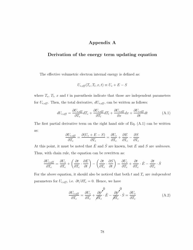
Appendix A

Derivation of the energy term updating equation

The effective volumetric electron internal energy is defined as:

Ue,eff(Te, Tl, x, t) ≡ Ue + E − S

where Te, Tl, x and t in parenthesis indicate that those are independent parameters

for Ue,eff . Then, the total derivative, dUe,eff , can be written as follows:

dUe,eff =∂Ue,eff

∂TedTe +

∂Ue,eff

∂TldTl +

∂Ue,eff

∂xdx +

∂Ue,eff

∂tdt (A.1)

The first partial derivative term on the right hand side of Eq. (A.1) can be written

as:∂Ue,eff

∂Te=

∂(Ue + E − S)

∂Te=

∂Ue

∂Te+

∂E

∂Te−

∂S

∂Te

At this point, it must be noted that E and S are known, but E and S are unknown.

Thus, with chain rule, the equation can be rewritten as:

∂Ue,eff

∂Te=

∂Ue

∂Te+

(

∂t

∂Te·∂E

∂t

)

−(

∂t

∂Te·∂S

∂t

)

=∂Ue

∂Te+

∂t

∂Te· E −

∂t

∂Te· S

For the above equation, it should also be noticed that both t and Te are independent

parameters for Ue,eff , i.e. ∂t/∂Te = 0. Hence, we have

∂Ue,eff

∂Te=

∂Ue

∂Te+

!!

!!"0

∂t

∂Te· E −

!!

!!"0

∂t

∂Te· S =

∂Ue

∂Te(A.2)

78

79

In similar manner, noting that Ue is only Te dependent by definition, other derivatives

can also be evaluated as follows:

∂Ue,eff

∂Tl=

!!

!!"0

∂Ue

∂Tl+

!!

!!"0

∂t

∂Tl· E −

!!

!!"0

∂t

∂Tl· S = 0 (A.3)

∂Ue,eff

∂x=

!!

!!"0

∂Ue

∂x+

####$0

∂t

∂x· E −

####$0

∂t

∂x· S = 0 (A.4)

∂Ue,eff

∂t=

!!

!!"0

∂Ue

∂t+

####$1

∂t

∂t· E −

####$1

∂t

∂t· S = E − S (A.5)

By plugging equations from (A.2) to (A.5) into Eq. (A.1), we have

dUe,eff =∂Ue

∂TedTe +

(

E − S)

· dt

or, in discretized form,

∆Ue,eff =∂Ue

∂Te∆Te +

(

E − S)

· ∆t

Appendix B

Derivation of the heat flux term updating equation

To obtain the update relation for ∂$q/∂T , Eq. (3.3) can be partially differentiated

with respect to Te as follow:

∂

∂Te

(

τe∂qe,x

∂t+ qe,x

)

=∂

∂Te

(

−ke ·∂Te

∂x

)

Noting that ke and τe can be explicitly expressed in terms of Te, for example Eqs. (2.5)

and (3.6) respectively, we have

∂τe

∂Te

∂qe,x

∂t+ τe

∂

∂Te

(

∂qe,x

∂t

)

+∂qe,x

∂Te= −

∂ke

∂Te

∂Te

∂x− ke

∂

∂Te

(

∂Te

∂x

)

It is clear that the second term on the right side can be eliminated as follow:

ke∂

∂Te

(

∂Te

∂x

)

= ke∂

∂x

(

∂Te

∂Te

)

= ke∂

∂x%%

%%%&

1(

∂Te

∂Te

)

= 0

Hence, by rearrangement and defining ∂qe,x/∂Te ≡ Ψ, we have a discretized equation

as

τeΨt+∆t − Ψt

∆t+ Ψt+∆t = −

(

∂ke

∂Te

∂Te

∂x+

∂τe

∂Te

∂qe,x

∂t

)

By rearrangement and discretizing the ∂qe,x/∂t term,

Ψt+∆t =1

τe + ∆t·(

τe · Ψt −∂τe

∂Te·(

qt+∆te,x − qt

e,x

)

− ∆t ·∂ke

∂Te

∂Te

∂x

)

(B.1)

Noting that qte,x is known to the user subroutine, if Eq. (2.15) is substituted into

Eq. (B.1), we obtain

Ψt+∆t =1

τe + ∆t·(

τe · Ψt +∂τe

∂Te

∆t

τe + ∆t

(

qte,x + ke

∂Te

∂x

)

− ∆t ·∂ke

∂Te·∂Te

∂x

)

(B.2)

80

81

It is clear that Eq. (B.2) is identical to Eq. (2.16) if (∂q/∂T )te,x replaces Ψt.

Similarly, for ∂$q/∂(∇T ), Eq. (2.4) can be partially differentiated with respect to

∂Te/∂x as follow:

∂

∂(∂Te/∂x)

(

τe∂qe,x

∂t+ qe,x

)

=∂

∂(∂Te/∂x)

(

−ke ·∂Te

∂x

)

Assuming that ke and τe are independent of temperature gradient, it can be written

as

τe ·∂

∂(∂Te/∂x)

(

∂qe,x

∂t

)

+∂qe,x

∂(∂Te/∂x)= −ke ·

∂(∂Te/∂x)

∂(∂Te/∂x)

By rearrangement and defining ∂qe,x/∂(∂Te/∂x) ≡ Ξ, we have

τe ·∂Ξ

∂t+ Ξ = −ke

which can be discretized as

τe ·Ξt+∆t − Ξt

∆t+ Ξt+∆t = −ke

and can be rearranged as

Ξt+∆t =1

τe + ∆t·(

τe · Ξt −∆t · ke

)

(B.3)

Again, it is clear that Eq. (B.3) is identical to Eq. (2.17) if (∂q/∂(∇T ))te,x replaces

Ξt.

Appendix C

Source codes of ABAQUS user subroutines

The user subroutine UMATHT codes equations from Eq. (2.12) to Eq. (2.17). In

the subroutine, the variables “ztp”, “zfln”, “zrfl” and “zskd” in lines 13 ∼ 16 define

pulse duration in ps, input fluence in J/cm2, reflectivity, and the skin depth in nm,

respectively. The source code is listed as follows:

1 SUBROUTINE UMATHT(U,DUDT,DUDG,FLUX,DFDT,DFDG,STATEV,TEMP,2 $ DTEMP,DTEMDX,TIME,DTIME,PREDEF,DPRED,CMNAME,NTGRD,NSTATV,3 $ PROPS,NPROPS,COORDS,PNEWDT,NOEL,NPT,LAYER,KSPT,KSTEP,KINC)4 c

5 INCLUDE ’ABAPARAM. INC ’6 c

7 CHARACTER∗80 CMNAME8 c

9 DIMENSION DUDG(NTGRD) ,FLUX(NTGRD) ,DFDT(NTGRD) ,10 $ DFDG(NTGRD,NTGRD) ,STATEV(NSTATV) ,DTEMDX(NTGRD) ,TIME(2 ) ,11 $ PREDEF(1 ) ,DPRED(1 ) ,PROPS(NPROPS) ,COORDS(3)12 c

13 ztp = 0 .514 z f l n = 0.40015 z r f l = 0.33216 zskd = 14.517 c

18 cond = STATEV(1)19 dkdtemp = STATEV(2)20 specht = STATEV(3)21 edot = STATEV(4)22 taue = STATEV(5)23 dtaue = STATEV(6)24 c

25 DUDT = specht26 taud = DTIME + taue27 c

82

83

28 i f (CMNAME(1 : 4 ) . eq . ’MATE’ ) then

29 c

30 t t = TIME(2) + DTIME31 xx = COORDS(1)32 zpp = (1− z r f l ) ∗ ( z f l n ∗ ( 1 . 0 e7 ) ) / ztp33 sdot = zpp ∗ s tg ( tt , ztp ) ∗ sxe (xx , zskd )34 c

35 du = DUDT∗DTEMP + ( edot − sdot )∗DTIME36 U = U + du37 c

38 do i =1, NTGRD39 FLUX( i ) = (FLUX( i )∗ taue−DTIME∗cond∗DTEMDX( i ) )/ taud40 DFDG( i , i ) = (DFDG( i , i )∗ taue−DTIME∗cond )/ taud41 DFDT( i ) =(DFDT( i )∗ taue42 # +dtaue ∗(DTIME/taud )∗ ( cond∗DTEMDX( i )+FLUX( i ) )43 # −DTIME∗dkdtemp∗DTEMDX( i ) )/ taud44 end do

45 c

46 else

47 c

48 du = DUDT∗DTEMP − edot ∗DTIME49 U = U + du50 c

51 do i =1, NTGRD52 FLUX( i ) = −cond∗DTEMDX( i )53 DFDG( i , i ) = −cond54 end do

55 end i f

56 c

57 RETURN

58 END

The user subroutine USDFLD codes material properties and temperature infor-

mation sharing, Fig. 2.2 (a). These are defined in lines 13 and 14:

1 SUBROUTINE USDFLD(FIELD,STATEV,PNEWDT,DIRECT,T,CELENT,2 1 TIME,DTIME,CMNAME,ORNAME,NFIELD,NSTATV,NOEL,NPT,LAYER,3 2 KSPT,KSTEP,KINC,NDI ,NSHR,COORD,JMAC,JMATYP,MATLAYO,LACCFLA)4 c

5 INCLUDE ’ABAPARAM. INC ’6 c

7 CHARACTER∗80 CMNAME,ORNAME8 CHARACTER∗3 FLGRAY(15)9 DIMENSION FIELD(NFIELD) ,STATEV(NSTATV) ,DIRECT( 3 , 3 ) ,

10 1 T(3 , 3 ) ,TIME(2)11 DIMENSION ARRAY(15) ,JARRAY(15) ,JMAC(∗ ) ,JMATYP(∗ ) ,COORD(∗ )

84

12 c

13 DIMENSION ztmpl (350 ,4 ) , ztmpe (350 ,4 )14 COMMON / z t l / ztmpl , ztmpe15 c

16 CALL GETVRM( ’TEMP’ ,ARRAY,JARRAY,FLGRAY,JRCD,JMAC,JMATYP,MATLAYO,17 1 LACCFLA)18 c

19 i f (CMNAME(1 : 4 ) . eq . ’MATE’ ) then

20 tmpl = ztmpl (NOEL,NPT)21 i f ( (KSTEP . eq . 1) . and . (KINC . eq . 0 ) ) tmpl = 0 .322 tmpe = ARRAY(1)23 c

24 STATEV(1) = cne ( tmpe , tmpl )25 STATEV(2) = dcnedt ( tmpe , tmpl )26 STATEV(3) = sphte ( tmpe )27 c

28 ztmpe (NOEL,NPT) = tmpe29 c

30 else

31 c

32 ne l = NOEL − 60033 c

34 tmpe = ztmpe ( nel ,NPT)35 i f ( (KSTEP . eq . 1) . and . (KINC . eq . 0 ) ) tmpe = 0.336 tmpl = ARRAY(1)37 c

38 STATEV(1) = 0 .039 STATEV(2) = 0 .040 STATEV(3) = sph t l ( tmpl )41 c

42 ztmpl ( nel ,NPT) = tmpl43 c

44 end i f45 c

46 ca l l c p l f ( gg , dgdtmp , tmpe , tmpl )47 STATEV(4) = gg ∗ ( tmpe − tmpl )48 c

49 ca l l tauc ( tu , dtu , tmpe , tmpl )50 STATEV(5) = tu51 STATEV(6) = dtu52 c

53 RETURN

54 END

The user subroutine UMESHMOTION calculates domain deformation due to ab-

lation using Eq. (2.19). The results are then converted from normalized coordinates

85

to actual coordinates, Fig. 2.3, in lines 37 ∼ 40, and the value passed to ABAQUS,

lines 46 and 47:

1 SUBROUTINE UMESHMOTION(UREF,ULOCAL,NODE,NNDOF,2 ∗ LNODETYPE,ALOCAL,NDIM,TIME,DTIME,PNEWDT,3 ∗ KSTEP,KINC,KMESHSWEEP,JMATYP,JGVBLOCK,LSMOOTH)4 c

5 INCLUDE ’ aba param . inc ’6 c

7 parameter ( t c r i t = 6 .903)8 c

9 DIMENSION ULOCAL(NDIM) , JELEMLIST(100)10 DIMENSION ALOCAL(NDIM,∗ ) ,TIME(2)11 DIMENSION JMATYP(∗ ) ,JGVBLOCK(∗ )12 c

13 dimension array (10)14 c

15 i f (NODE . l t . 600) then

16 ndt1 = NODE + 60017 ndx1 = NODE18 else

19 ndt1 = NODE20 ndx1 = NODE21 end i f

22 c

23 ndt2 = ndt1 + 124 ndx2 = ndx1 + 125 l t r n = 026 c

27 ca l l GETVRN( ndt1 , ’NT’ , array , j r cd ,JGVBLOCK, l t r n )28 tmp1 = array (1)29 ca l l GETVRN(ndx1 , ’COORD’ , array , j r cd ,JGVBLOCK, l t r n )30 crd1 = array (1)31 ca l l GETVRN( ndt2 , ’NT’ , array , j r cd ,JGVBLOCK, l t r n )32 tmp2 = array (1)33 ca l l GETVRN(ndx2 , ’COORD’ , array , j r cd ,JGVBLOCK, l t r n )34 crd2 = array (1)35 c

36 i f ( tmp1 . gt . t c r i t ) then

37 xxx = (tmp1 + tmp2 − 2 ∗ t c r i t )/ ( tmp1 − tmp2)38 xx1 = ( xxx + 1) ∗ ( crd2 − crd1 ) / 239 x2 = 0.040 x1 = max( 0 . 0 , xx1 )41 else

42 x1 = 0.043 x2 = 0.0

86

44 end i f

45 c

46 ULOCAL(1) = x1 ∗ ALOCAL(1 ,1 ) + x2 ∗ ALOCAL(2 ,1 )47 ULOCAL(2) = x1 ∗ ALOCAL(1 ,2 ) + x2 ∗ ALOCAL(2 ,2 )48 c

49 LSMOOTH = 150 c

51 RETURN

52 END

Bibliography

87

Bibliography

Kaganov, M., Lifshitz, I. and Tanatarov, L., 1957, “Relaxation between electrons andthe crystalline lattice,” Sov Phys-JETP, 4, pp. 173–178

Gregg, D. and Thomas, S., 1966, “Momentum transfer produced by focused lasergiant pulses,” J Appl Phys, 37(7), pp. 2787 – 2788

Anderholm, N., 1970, “Laser-generated stress waves,” Appl Phys Lett, 16(3), pp. 113– 115

Touloukian, Y.S. and DeWitt, D.P. (eds.), 1970, Thermophisical Properties of Matter,IFI/PLENUM, New York, New York

Dabby, F. and Paek, U., 1972, “High-intensity laser-induced vaporization and explo-sion of solid material,” IEEE J Quantum Electron, QE 8, pp. 106–111

Fairand, B., Wilcox, B., Gallagher, W. and Williams, D., 1972, “Laser shock-inducedmicrostructural and mechanical property changes in 7075 aluminum,” J Appl Phys,43(9), pp. 3893 – 3895

Anisimov, S.I., Kapeliovich, B.L. and Perel’man, T.L., 1974, “Electron emission frommetal surfaces exposed to ultrashort laser pulses,” Sov Phys-JETP, 39(2), pp. 375– 377

Ashcroft, N. and Mermin, N., 1976, Solid state physics, Thomson learning Inc., USA

Strickland, D. and Mourou, G., 1985, “Compression of amplified chirped opticalpulses,” Opt Commun, 56, pp. 219–221

Siegman, A.E., 1986, LASERS, University Science Books, Sausalito, Calinfornia

Allen, P., 1987, “Theory of thermal relaxation of electrons in metals,” Phys Rev Lett,59, pp. 1460–1463

Elsayedali, H., Norris, T., Pessot, M. and Mourou, G., 1987, “Time-resolved observa-tion of electron-phonon relaxation in copper,” Phys Rev Lett, 58, pp. 1212–1215

Korb, L.J. and Olson, D.L. (eds.), 1987, ASM Handbook, vol. 13, ASM International,Materials Park, Ohio

88

89

Sherman, N., Brunel, F., Corkum, P. and Hegmann, F., 1989, “Transient-response ofmetals to ultrashort pulse excitation,” Opt Eng, 28, pp. 1114–1121

Banas, G., Elsayed-Ali, H., Lawrence, F.V., J. and Rigsbee, J., 1990, “Laser shock-induced mechanical and microstructural modification of welded maraging steel,” JAppl Phys, 67(5), pp. 2380 – 2384

Brorson, S., Kazeroonian, A., Moodera, J., Face, D., Cheng, T., Ippen, E., Dressel-haus, M. and Dresselhaus, G., 1990, “Femtosecond room-temperature measurementof the electron-phonon coupling constant λ in metallic superconductors,” Phys RevLett, 64, pp. 2172–2175

Forget, P., Strudel, J., Jeandin, M., Lu, J. and Castex, L., 1990, “Laser shock surfacetreatment of Ni-based superalloys,” Mater Manuf Process, 5(4), pp. 501 – 528

Montgomery, D.C., 1991, Design and Analysis of Experiments, 3rd ed., John Wiley& Sons, Inc., Canada

Fann, W., Storz, R., Tom, H. and Bokor, J., 1992, “Direct measurement of nonequilib-rium electron-energy distributions in subpicosecond laser-heated gold films,” PhysRev Lett, 68(18), pp. 2834 – 2837

Mills, A.F., 1992, Heat Transfer, Irwin Inc., Boston, Massachusetts

Qiu, T. and Tien, C., 1993, “Heat-transfer mechanisms during short-pulse laser-heating of metals,” Trans ASME, J Heat Transf, 115, pp. 835–841

Hays-Stang, K.J. and Haji-Sheikh, A., 1994, “An analytical solution for heat transferin thin films,” ASME Heat Transfer Div. Publ. HTD, vol. 293, Chicago, IL, USA,pp. 1 – 7

Wang, X., Riffe, D., Lee, Y. and Downer, M., 1994, “Time-resolved electron-temperature measurement in a highly excited gold target using femtosecondthermionic emission,” Phys Rev B, Condens Matter, 50, pp. 8016–8019

Preuss, S., Demchuk, A. and Stuke, M., 1995, “Sub-picosecond UV laser ablation ofmetals,” Appl Phys A, Mater Sci Process, 61(1), pp. 33 –37

Pronko, P., Dutta, S., Du, D. and Singh, R., 1995, “Thermophysical effects in laserprocessing of materials with picosecond and femtosecond pulses,” J Appl Phys, 78,pp. 6233–6240

Chichkov, B., Momma, C., Nolte, S., vonAlvensleben, F. and Tunnermann, A., 1996,“Femtosecond, picosecond and nanosecond laser ablation of solids,” Appl Phys A,Mater Sci Process, 63, pp. 109–115

Huttner, B. and Rohr, G., 1996, “On the theory of ps and sub-ps laser pulse interac-

90

tion with metals .1. surface temperature,” Appl Surf Sci, 103, pp. 269–274

Kelly, R. and Miotello, A., 1996, “Comments on explosive mechanisms of laser sput-tering,” Appl Surf Sci, 96-8, pp. 205–215

Peyre, P., Fabbro, R., Merrien, P. and Lieurade, H., 1996, “Laser shock processing ofaluminium alloys. application to high cycle fatigue behaviour,” Mater Sci Eng A,A210(1-2), pp. 102 – 113

Stuart, B., Feit, M., Herman, S., Rubenchik, A., Shore, B. and Perry, M., 1996,“Optical ablation by high-power short-pulse lasers,” J Opt Soc Am B, Opt Phys,13, pp. 459–468

Anisimov, S. and Rethfeld, B., 1997, “On the theory of ultrashort laser pulse inter-action with a metal,” Proc. SPIE, vol. 3093, pp. 192 – 203

Liu, X., Du, D. and Mourou, G., 1997, “Laser ablation and micromachining withultrashort laser pulses,” IEEE J Quantum Electron, 33, pp. 1706–1716

Momma, C., Nolte, S., Chichkov, B., vonAlvensleben, F. and Tunnermann, A., 1997,“Precise laser ablation with ultrashort pulses,” Appl Surf Sci, 109/110, pp. 15–19

Nolte, S., Momma, C., Jacobs, H., Tunnermann, A., Chichkov, B., Wellegehausen,B. and Welling, H., 1997, “Ablation of metals by ultrashort laser pulses,” J OptSoc Am B, 14, pp. 2716–2722

Tzou, D., 1997, Macro- to Microscale Heat Transfer, Taylor & Francis, Washington,DC

Craciun, V., Craciun, D., Bunescu, M., Boulmer-Leborgne, C. and Hermann, J., 1998,“Subsurface boiling during pulsed laser ablation of Ge,” Phys Rev B, CondensMatter, 58, pp. 6787–6790

Fabbro, R., Peyre, P., Berthe, L. and Scherpereel, X., 1998, “Physics and applicationsof laser-shock processing,” J Laser Appl, 10(6), pp. 265 – 279

Hong, Z. and Chengye, Y., 1998, “Laser shock processing of 2024-T62 aluminumalloy,” Mater Sci Eng A, 257(2), pp. 322 – 327

Smith, A. and Norris, M., 1998, “Numerical solution for the diffusion of high intensity,ultrashort laser pulses within metal films,” Proceedings of 11th International HeatTransfer Conference, vol. 5, Kyongju, Korea, pp. 241–246

Braisted, W. and Brockman, R., 1999, “Finite element simulation of laser shockpeening,” Int J Fatigue, 21(7), pp. 719 – 724

Chu, J., Rigsbee, J., Banas, G. and Elsayed-Ali, H., 1999, “Laser-shock processing

91

effects on surface microstructure and mechanical properties of low carbon steel,”Mater Sci Eng A, A260(1-2), pp. 260 – 268

Furusawa, K., Takahashi, K., Kumagai, H., Midorikawa, K. and Obara, M., 1999,“Ablation characteristics of Au, Ag, and Cu metals using a femtosecond Ti:sapphirelaser,” Appl Phys A, Mater Sci Process, 69 [Suppl.], pp. S359–S366

Hostetler, J., Smith, A., Czajkowsky, D. and Norris, P., 1999, “Measurement of theelectron-phonon coupling factor dependence on film thickness and grain size in Au,Cr, and Al,” Appl Opt, 38, pp. 3614–3620

Smith, A., Hostetler, J. and Norris, P., 1999, “Nonequilibrium heating in metal films:An analytical and numerical analysis,” Numer Heat Transf A, Appl, 35, pp. 859–873

Wellershoff, S., Hohlfeld, J., Gudde, J. and Matthias, E., 1999, “The role of electron-phonon coupling in femtosecond laser damage of metals,” Appl Phys A, Mater SciProcess, 69, pp. S99–S107

Zhu, X., Naumov, A., Villeneuve, D. and Corkum, P., 1999, “Influence of laser pa-rameters and material properties on micro drilling with femtosecond laser pulses,”Appl Phys A, Mater Sci Process, 69 [Suppl.], pp. S367–S371

Banks, P.S., Feit, M.D., Perry, M.D., Stuart, B.C., Rubenchik, A.M. and Komashko,A.M., 2000, “Femtosecond laser materials processing,” Proc. SPIE, vol. 3934, pp.14 –21

Hammersley, G., Hackel, L. and Harris, F., 2000, “Surface prestressing to improvefatigue strength of components by laser shot peening,” Opt Lasers Eng, 34(4-6),pp. 327 – 337

Hohlfeld, J., Wellershoff, S., Gudde, J., Conrad, U., Jahnke, V. and Matthias, E.,2000, “Electron and lattice dynamics following optical excitation of metals,” ChemPhys, 251, pp. 237–258

Kaspar, J., Luft, A. and Skrotzki, W., 2000, “Deformation modes and structureevolution in laser-shock-loaded molybdenum single crystals of high purity,” CrystRes Technol, 35(4), pp. 437 – 448

Peyre, P., Scherpereel, X., Berthe, L., Carboni, C., Fabbro, R., Beranger, G. andLemaitre, C., 2000, “Surface modifications induced in 316L steel by laser peeningand shot-peening. influence on pitting corrosion resistance,” Mater Sci Eng A,A280(2), pp. 294 – 302

Chen, J. and Beraun, J., 2001, “Numerical study of ultrashort laser pulse interactionswith metal films,” Numer Heat Transf A, Appl, 40, pp. 1–20

92

Jou, D., Casas-Vazquez, J. and Lebon, G., 2001, Extended Irreversible Thermody-namics, Springer-Verlag, Germany

Kalpakjian, S. and Schmid, S., 2001, Manufacturing Processes for Engineering Ma-terials, 4th ed., Pearson Education, Upper Saddle River, New Jersey

Kaspar, J. and Luft, A., 2001, “Microstructure formed in body centred cubic metalsby laser shock processing,” Surf Eng, 17(5), pp. 379 – 383

Wild, M., Gillner, A. and Poprawe, R., 2001, “Locally selective bonding of siliconand glass with laser,” Sens Actuators A Phys, 93(1), pp. 63 – 69

Brockmann, R., Honekamp, M., Dickmann, K., Meier, S., Letsch, H. and Matthes,K.J., 2002, “Modern welding processes for microsystems engineering and electronicstaking particular account of the laser,” Weld Res Abroad, 48(4), pp. 27 – 32

Chen, J., Latham, W. and Beraun, J., 2002, “Axisymmetric modeling of femtosecond-pulse laser heating on metal films,” Numer Heat Transf B, Fundam, 42, pp. 1–17

Dickinson, J., 2002, “Physical and chemical aspects of laser-materials interactionsrelevant to laser processing,” Proc. SPIE, vol. 4637, pp. 453 – 464

Du, J., Longobardi, J., Latham, W. and Kar, A., 2002, “Laser marginal lap microw-elding for ultrathin sheet metal,” J Laser Appl, 14(1), pp. 4 – 8

Dumitru, G., Romano, V., Weber, H., Sentis, M. and Marine, W., 2002, “Femtosecondablation of ultrahard materials,” Appl Phys A, Mater Sci Process, 74, pp. 729–739

Hecht, E., 2002, Optics, 4th ed., Addison Wesley, San Francisco, California

Kramer, T., Olowinsky, A. and Durand, F., 2002, “Shadow-a new welding technique,”Proc. SPIE, vol. 4637, pp. 545 – 554

Montross, C., Wei, T., Ye, L., Clark, G. and Mai, Y.W., 2002, “Laser shock processingand its effects on microstructure and properties of metal alloys: a review,” Int JFatigue, 24(10), pp. 1021 – 1036

Schmidt, V., Husinsky, W. and Betz, G., 2002, “Ultrashort laser ablation of metals:pump-probe experiments, the role of ballistic electrons and the two-temperaturemodel,” Appl Surf Sci, 197, pp. 145–155

See, D., Dulaney, J., Clauer, A. and Tenaglia, R., 2002, “The air force manufacturingtechnology laser peening initiative,” Surf Eng, 18(1), pp. 32 – 36

Abe, N., Funada, Y. and Ishide, M., 2003, “Micro-welding of thin foil with directdiode laser,” Proc. SPIE, vol. 5063, pp. 287 – 291

93

Chen, J. and Beraun, J., 2003, “Modelling of ultrashort laser ablation of gold filmsin vacuum,” J Opt A:Pure Appl Opt, 5, pp. 168–173

Deshayes, Y., Bechou, L., Deletage, J., Verdier, F., Danto, Y., Laffitte, D. andGoudard, J., 2003, “Three-dimensional fem simulations of thermomechanicalstresses in 1.55 µm laser modules,” Microelectron Reliab, 43(7), pp. 1125 – 1136

Dijken, D., Hoving, W. and De Hosson, J., 2003, “Laser penetration spike welding: amicrolaser welding technique enabling novel product designs and constructions,” JLaser Appl, 15(1), pp. 11 – 18

Griffith, M.L., Ensz, M.T. and Reckaway, D.E., 2003, “Femtosecond laser machiningof steel,” Proc. SPIE, vol. 4977, pp. 118 –122

Park, S., Ohmura, E. and Miyamoto, I., 2003, “Micro welding of ultra thin metal foilusing yb-fiber laser,” Proc. SPIE, vol. 4830, pp. 52 – 56

Peyre, P., Sollier, A., Chaieb, I., Berthe, L., Bartnicki, E., Braham, C. and Fabbro,R., 2003, “FEM simulation of residual stresses induced by laser peening,” Eur PhysJ AP, 23, pp. 83–88

Semak, V., Knorovsky, G. and MacCallum, D., 2003, “On the possibility of microw-elding with laser beams,” J Phys D:Appl Phys, 36(17), pp. 2170 – 2174

Sonntag, R.E., Borgnakke, C. and Wylen, G.J.V., 2003, Fundamentals of Thermody-namics, 6th ed., John Wiley & Sons, Inc., Hoboken, New Jersey

Triantafyllidis, D., Schmidt, M. and Li, L., 2003, “Comparison of high power diodelaser and Nd:YAG laser microwelding of k-type thermocouples,” J Mater ProcessTechnol, 138, pp. 102–108

Yilbas, B., Shuja, S., Arif, A. and Gondal, M., 2003, “Laser-shock processing of steel,”J Mater Process Technol, 135(1), pp. 6 – 17

Zhang, X. and Xu, X., 2003, “High precision microscale bending by pulsed and cwlasers,” Trans ASME, J Manuf Sci Eng, 125, pp. 512–518

Bulgakova, N., Bulgakov, A. and Babich, L., 2004, “Energy balance of pulsed laserablation: thermal model revised,” Appl Phys A, Mater Sci Process, 79, pp. 1323–1326

Duley, W., 2004, “Physics, chemistry, and laser microprocessing,” J Laser Appl,16(1), pp. 52 – 54

Isamu, M., Takeshi, K., Park, S., Hiroaki, U., Koji, W. and Toshihiko, O., 2004,“Applications of single-mode fiber-lasers to novel microwelding,” Proc. SPIE, vol.5662, pp. 507 – 514

94

Rubio-Gonzalez, C., Ocana, J., Gomez-Rosas, G., Molpeceres, C., Paredes, M., Ban-deras, A., Porro, J. and Morales, M., 2004, “Effect of laser shock processing onfatigue crack growth and fracture toughness of 6061-T6 aluminum alloy,” MaterSci Eng A, A386(1-2), pp. 291 – 295

Tan, Y., Wu, G., Yang, J. and Pan, T., 2004, “Laser shock peening on fatigue crackgrowth behaviour of aluminium alloy,” Fatigue Fract Eng Mater Struct, 27, pp.649–656

Vander Voort, G.F. (ed.), 2004, ASM Handbook, vol. 9, ASM International, MaterialsPark, Ohio

Yakimets, I., Richard, C., Beranger, G. and Perye, P., 2004, “Laser peening processingeffect on mechanical and tribological properties of rolling steel 100Cr6,” Wear,256(3-4), pp. 311 – 320

Zhang, W., Yao, Y. and Noyan, I., 2004, “Microscale laser shock peening of thin films,part 2: High spatial resolution material characterization,” Trans ASME, J ManufSci Eng, 126(1), pp. 18 – 24

Aldajah, S., Ajayi, O., Fenske, G. and Xu, Z., 2005, “Effect of laser surface mod-ifications tribological performance of 1080 carbon steel,” Trans ASME, J Tribol,127(3), pp. 596 – 604

Borrisutthekul, R., Miyashita, Y. and Mutoh, Y., 2005, “Dissimilar material laserwelding between magnesium alloy az31b and aluminum alloy a5052-o,” Sci TechnolAdv Mater, 6, pp. 199–204

Chen, J., Latham, W. and Beraun, J., 2005, “The role of electron-phonon couplingin ultrafast laser heating,” J Laser Appl, 17, pp. 63–68

Fabbro, R., Slimani, S., Coste, F. and Briand, F., 2005, “Study of keyhole behaviourfor full penetration Nd-Yag CW laser welding,” J Phys D:Appl Phys, 38, pp. 1881–1887

Lin, Y., Eichele, C. and Shi, F., 2005, “Effect of welding sequence on welding-induced-alignment-distortion in packaging of butterfly laser diode modules: Simulation andexperiment,” J Lightwave Technol, 23, pp. 615–623

Vogel, A., Noack, J., Huttman, G. and Paltauf, G., 2005, “Mechanisms of femtosecondlaser nanosurgery of cells and tissues,” Appl Phys B, Lasers Opt, B81(8), pp. 1015– 1047

ABAQUS Inc., 2006, ABAQUS Manual, Providence, Rhode Island, version 6.6 ed.

Cao, X., Jahazi, M., Immarigeon, J. and Wallace, W., 2006, “A review of laser weldingtechniques for magnesium alloys,” J Mater Process Technol, 171, pp. 188–204

95

Dehoux, T., Perton, M., Chigarev, N., Rossignol, C., Rampnoux, J.M. and Audoin,B., 2006, “Effect of laser pulse duration in picosecond ultrasonics,” J Appl Phys,100(6), pp. 064318–1 – 064318–8

Farrahi, G. and Ghadbeigi, H., 2006, “An investigation into the effect of varioussurface treatments on fatigue life of a tool steel,” J Mater Process Technol, 174(1-3), pp. 318 – 324

Lin, Z. and Zhigilei, L.V., 2006, “Thermal excitation of d band electrons in au:Implications for laser-induced phase transformations,” Proc. SPIE, vol. 6261, pp.62610U–1 – 62610U–14

Mys, I. and Schmidt, M., 2006, “Laser micro welding of copper and aluminum,” Proc.SPIE, vol. 6107, pp. 610703–1 – 610703–6

Tamaki, T., Watanabe, W. and Itoh, K., 2006, “Laser micro-welding of transparentmaterials by a localized heat accumulation effect using a femtosecond fiber laser at1558 nm,” Opt Express, 14, pp. 10460–10468

Zhang, H. and Senkara, J., 2006, Resistance Welding, Taylor & Francis, Boca Raton,Florida

Richter, K., Behr, W. and Reisgen, U., 2007, “Low heat welding of titanium materialswith a pulsed Nd:YAG laser,” Materwis Werkstofftech, 38, pp. 51–56

Sierra, G., Peyre, P., Deschaux-Beaume, F., Stuart, D. and Fras, G., 2007, “Steel toaluminium key-hole laser welding,” Mater Sci Eng A, 447(1-2), pp. 197 – 208