FEA of Nonlinear Problems
62
FINITE ELEMENT ANALYSIS OF NONLINEAR PROBLEMS SCRIPT OF LECTURES Doc. Ing. Vladimír Ivančo, PhD. Faculty of Mechanical Engineering, Technical University of Košice, Slovakia HS Wismar, June 2010
-
Upload
michel-zeicher -
Category
Documents
-
view
329 -
download
4
Transcript of FEA of Nonlinear Problems

FINITE ELEMENT ANALYSIS
OF NONLINEAR PROBLEMS
SCRIPT OF LECTURES
Doc. Ing. Vladimír Ivančo, PhD.
Faculty of Mechanical Engineering, Technical University of Košice, Slovakia
HS Wismar, June 2010

2 FINITE ELEMENT ANALYSIS OF NONLINEAR PROBLEMS
CONTENTS
1. Structural nonlinearities .......................................................................4
1.1 Introduction.......................................................................................4
1.2 Types of structural nonlinearities......................................................5
1.3 Concept of time curves .....................................................................5
2. Geometrically nonlinear finite element analysis .................................7
2.1 Large displacement and small strain behavior ..................................7
2.2 Incremental - iterative solutions......................................................13
2.2.1 Incremental method...........................................................15
2.2.2 Newton-Raphson method..................................................16
2.2.3 Modified Newton-Raphson method..................................18
2.2.4 Quasi-Newton methods.....................................................18
2.3 Linear stability analysis ..................................................................18
2.4 Large displacement and large strain behaviour...............................20
2.4.1 Total Lagrangian formulation ...........................................20
2.4.2 Updated Lagrangian formulation ......................................20
3. Material nonlinearities .......................................................................21
3.1 Introduction.....................................................................................21
3.2 Nonlinear elasticity models.............................................................21
3.3 Elastoplastic material model ...........................................................23
3.3.1 Yielding criterion ..............................................................23
3.3.2 Post yielding behaviour.....................................................26
3.3.3 Constitutional equations of elastoplastic material.............28
3.3.4 Integration of constitutive equations.................................30
3.3.4.1 Generalised trapezoidal rule................................................31 3.3.4.2 Generalised mid point rule..................................................31
3.3.5 Numerical procedures .......................................................32
Appendix............................................................................................................34
Nonlinear analyses with COSMOS/M program..........................................35
1.1 Properties of finite elements ................................................35
1.2 Nonlinear analysis setup ......................................................38
1.3 Time curves and time parameters ........................................44
1.4 Restart possibilities ..............................................................49

FINITE ELEMENT ANALYSIS OF NONLINEAR PROBLEMS 3
Examples of COSMOS/M program use ..................................................... 50
1.5 Compressed slender beam ................................................... 50
1.6 Thick-walled pipe subjected to internal pressure ................ 53
1.7 Deformation of a thin-walled tank ...................................... 56

4 FINITE ELEMENT ANALYSIS OF NONLINEAR PROBLEMS
1. STRUCTURAL NONLINEARITIES
1.1 Introduction
Many engineering problems can be solved using a linear approximation. In the Finite Element Analysis (FEA) the set of equations, describing the structural behaviour is then linear
FdK = (1.1)
In this matrix equation, K is the stiffness matrix of the structure, d is the nodal
displacements vector and F is the external nodal force vector.
Characteristics of linear problems is that
• the displacements are proportional to the loads,
• the stiffness of the structure is independent on the value of the load level.
Though behaviour of real structures is nonlinear, e.g. displacements are not proportional to the loads; nonlinearities are usually unimportant and may be neglected in most practical problems.
The set of linear algebraic equations (1.1) is received if assuming that
• displacements are small and can be neglected in equilibrium equations,
• the strain is proportional to the stress (linear Hookean material model),
• loads are conservative, independent on displacements, and supports of the structure remain unchanged.
Solution of many problems needs abandonment of these approximations. The
displacements may be so large changes of the structure shape (or configuration changes) cannot be neglected. Many materials behave nonlinearly or linear material model cannot be used if stress exceeds some value. Moreover, loads may change their orientations according to displacements and restraints may change during loading. Consequently, structure behaves nonlinearly. If these phenomena are included in a FEA, the set of equilibrium equations becomes nonlinear.

FINITE ELEMENT ANALYSIS OF NONLINEAR PROBLEMS 5
1.2 Types of structural nonlinearities
Structural nonlinearities can be specified as
1. Geometrical nonlinearities: The effect of large displacements on the overall geometric configuration of the structure.
2. Material nonlinearities: Material behaviour is nonlinear. Possible material models are:
a) nonlinear elastic,
b) elastoplastic,
c) viscoelastic,
d) viscoplastic.
3. Boundary nonlinearities, i.e. displacement dependent boundary conditions. The most frequent boundary nonlinearities are encountered in contact problems.
Consequences of nonlinear structural behaviour that have to be recognized are:
a) The principle of superposition cannot be applied. Thus, for example, the results of several load cases cannot be combined. Results of the nonlinear analysis cannot be scaled.
b) Only one load case can be handled at a time.
c) The sequence of application of loads (loading history) may be important. Especially, plastic deformations depend on a manner of loading. This is a reason for dividing loads into small increments in nonlinear FE analysis.
d) The structural behaviour can be markedly non-proportional to the applied load.
e) The initial state of stress (e.g. residual stresses from heat treatment, welding etc.) may be important.
1.3 Concept of time curves
For nonlinear static analysis, the loads are applied in incremental steps using time curves. The “time” variable represents a pseudo time, which denotes the intensity of the applied loads at certain step.
For nonlinear dynamic analysis and nonlinear static analysis with time-dependent material properties,1 “time” represents the real time associated with the loads’ application.
1 i.e. analysis of creep and relaxation problems by use of viscoelastic or viscoplastic material
models.

6 FINITE ELEMENT ANALYSIS OF NONLINEAR PROBLEMS
As an example, time curves of forces F1 and F2 loading simple beam are displayed in Figure 1.1. Values of forces at any time are defined as
( ) 111 ftF λ= and ( ) 222 ftF λ=
where f1 and f2 are nominal (input) values of forces and λ1 and λ1 are load
parameters that are functions of time t.
Figure 1.1: Example of time curves
The choice of time step size depends on several factors such as the level of
nonlinearities2 of the problem and the solution procedure. Generally, sufficiently small steps are necessary to simulate nonlinear response of a structure with satisfactory accuracy. On the other hand, large number of too small time steps uselessly increases consumption of CPU time. Computer programs are usually equipped with an adaptive automatic stepping algorithm to facilitate the analysis and to reduce the solution time demands.
2 Highly nonlinear problems need smaller load increments.

FINITE ELEMENT ANALYSIS OF NONLINEAR PROBLEMS 7
2. GEOMETRICALLY NONLINEAR
FINITE ELEMENT ANALYSIS
2.1 Large displacement and small strain behavior
To examine geometrically nonlinear behaviour we will start with an example. We assume large displacement, but small rotation and, what is the most important, small strain. The structure is very simple – only one bar truss as is shown in Figure 2.1. At the beginning, when the force P is zero, the axial force N in the bar is zero too and bar has its initial length L0.
Figure 2.1: Example of nonlinear structure – single bar truss
Using the free body diagram shown in Figure 2.1 the equilibrium equation is
0sin =− PN α or
.0=−+
PL
uhN (2.1)
Assume that material is linearly elastic with Young’s modulus E. The
assumption of small strains means here that changes of the bar cross sectional area A can be neglected. Then axial force in the bar is

8 FINITE ELEMENT ANALYSIS OF NONLINEAR PROBLEMS
ε0AEN = (2.2)
where A0 is the initial cross sectional area and ε is the engineering strain
defined as
0
0
L
LL −=ε . (2.3)
As lengths are given as
220 haL += and 22 )( uhaL ++= (2.4)
the expression for strain is getting rather complicated. We can overcame this
problem by introducing Green’s strain defined as
20
20
2
2L
LLG
−=ε (2.5)
which for our problem becomes
2
000 2
1
+=
L
u
L
u
L
hGε . (2.6)
Use of this new measure of strain is possible because we can define strain
arbitrarily. The only condition is that the strain measure must be objective, which means that is have to be independent on choice of coordinate system and insensitive to a rigid body movement. From equations (2.3) and (2.5), it follows that
+
−=
=
−+
+=
+=
+−=
−=
0
0
0
0
0
0
0
0
0
0
0
020
20
2
2
2
1
112
1
2
1
22
L
L
L
LL
L
LL
L
LL
L
LL
L
LL
L
LLG
ε
εεε
or
2
2
1εεε +=G . (2.7)
Noting that the constitution equation was measured as
εσ EA
N==
0 (2.8)

FINITE ELEMENT ANALYSIS OF NONLINEAR PROBLEMS 9
the same constitutive equation when using Green’s strain should be
GGGG
EEE ε
εε
εε
εε
εε
σ
2
11
2
1 2 +=
+== . (2.9)
This means that we should use value ])2/1(1/[ ε+=∗ EE instead of E in the constitution equation. Fortunately, we can ignore this complication now because for small engineering strain is the difference between engineering and Green’s strain negligible.
For example, consider that ε = 0,002 (e.g. mild steel yields at about this value), then εG = 0,002 + 0,5⋅0,0022 = 0,002002. This means that difference is only 0,1% i.e. a value that can be usually neglected. Assuming that strain is small, we can write GE εσ ≈ and according to equation (2.6)
+= 2
20
0
2
1uuh
L
AEN . (2.10)
Substituting (2.10) to equilibrium equation (2.1) and assuming that for small
strain is 0LL ≈ gives the equilibrium equation
( ) .232
22330
0 PuhuhuL
AE=++ 2.11)
Obviously, the equation is nonlinear with respect to displacement u. That means
that relation between load P and displacement u is represented not by a straight line as it is when changes of configuration are neglected but by a curve. This nonlinear characteristic for E = 2,1⋅105 MPa, A0 = 100 mm2, a = 200 mm and h = 20 mm is shown in Figure 2.2.

10 FINITE ELEMENT ANALYSIS OF NONLINEAR PROBLEMS
-1000
-500
0
500
1000
1500
2000
2500
-10 -5 0 5 10
u [mm]
P [N]
Figure 2.2: Geometrically nonlinear behaviour of a single bar truss
There is another possibility to obtain equation of equilibrium (2.1) or (2.11).
From principle of virtual displacements, it follows that when the structure is in equilibrium, virtual works of internal and external forces are equal for every
kinematically admissible set of virtual displacements. For our structure with one degree of freedom, only one virtual displacement uδ is possible and principle of virtual displacements has a form
uPV
V
G δδεσ =∫ d (2.12)
where Gδε is virtual strain corresponding to virtual displacement uδ . The
virtual strain can be expressed from equation (2.6) as
.2
1
d
d
d
d20
2
000u
L
uhu
L
u
L
u
L
h
uu
u
GG δδδ
εδε
+=
+== (2.13)
It is assumed in principle of virtual displacements that virtual displacement is
infinitesimal and hence the stress )/( AN=σ remains unchanged. Noting that σ and Gδε are constant over the whole volume V in this case and assuming that changes of the volume can be neglected due to small strain, i.e. 000 LAVV =≈ , equation (2.12) becomes

FINITE ELEMENT ANALYSIS OF NONLINEAR PROBLEMS 11
uPLAuL
uh
A
Nδδ =
+02
00
and from this equation it follows that
PL
uhN =
+
0
.
This is the same equation as the equation of equilibrium (2.1). After substituting
for N from (2.10) the equation (2.11) will be received again. Utilization of principle of virtual displacements (PVD) is a convenient way to
obtain conditions of equilibrium for complex structures. For general three-dimensional case we have three components of displacement u, v, w and six components of Green’s strain
∂∂
+
∂∂
+
∂∂
+∂∂
=222
2
1
x
w
x
v
x
u
x
uxε ,
∂∂
+
∂∂
+
∂∂
+∂∂
=222
2
1
y
w
y
v
y
u
y
vyε ,
∂∂
+
∂∂
+
∂∂
+∂∂
=222
2
1
z
w
z
v
z
u
z
wxε , (2.14)
y
w
x
w
y
v
x
v
y
u
x
u
x
v
y
uxy ∂
∂∂∂
+∂∂
∂∂
+∂∂
∂∂
+∂∂
+∂∂
=γ ,
z
w
x
w
z
v
x
v
z
u
x
u
x
w
z
uxz ∂
∂∂∂
+∂∂
∂∂
+∂∂
∂∂
+∂∂
+∂∂
=γ ,
z
w
y
w
z
v
y
v
z
u
y
u
y
w
z
vyz ∂
∂∂∂
+∂∂
∂∂
+∂∂
∂∂
+∂∂
+∂∂
=γ .
In finite element method are displacement interpolated within the finite
elements as
i
i
i uNu ∑= , i
i
i vNv ∑= , i
i
i wNw ∑= , (2.15)
where ui, vi, wi are nodal displacements and Ni are shape functions. Substituting
these equations into expressions of Green’s strain components, we obtain

12 FINITE ELEMENT ANALYSIS OF NONLINEAR PROBLEMS
dBBε )2
1( NL += . (2.16)
In matrix equation (2.16)
=
xy
xz
yz
z
y
x
γγγεεε
ε , (2.17)
and d is matrix of nodal displacements. Matrix LB is the usual small
displacement matrix and matrix NB reflects the fact that Green’s strain is a nonlinear function of displacements. Elements of this matrix are linear functions of nodal displacements d. It might be shown that virtual strain corresponding to the virtual nodal displacements dδ is
.)( dBdBBε δδδ =+= NL (2.18)
According to the principle of virtual displacements, virtual work of internal
forces must be equal to virtual work of external forces if the structure is in equilibrium. This is represented by the equation
FdσεT
V
T V δδ∫ =d (2.19)
where F is matrix of nodal forces. We suppose linear relation between stress and strain components, hence
Dεσ = where D is matrix of material elastic constants. Substituting (2.18) into (2.19) gives
FdσBdT T
V
T V δδ ∫ =d (2.20)
for any kinematically admissible set of virtual displacements dδ . Then
FσBT∫ =
V
Vd . (2.21)

FINITE ELEMENT ANALYSIS OF NONLINEAR PROBLEMS 13
The last equation is a matrix representation of a set of nonlinear algebraic equations for unknown nodal displacements d.
FdR =)( . (2.22)
2.2 Incremental - iterative solutions
We have seen that assumption of large displacements leads to nonlinear equation of equilibrium (2.1) or (2.11) for a simple bar truss example. Generally, in finite element analysis we have a set of nonlinear equations (2.22). Let us start with the bar-truss example. The equation of equilibrium (2.1) or (2.11) can be written in a form
PuR =)( (2.23)
where
( ).232
)( 223300
uhuhuL
AE
L
uhNuR ++=
+= (2.24)
represents a component of internal force.
The basic step to solve the nonlinear equation (2.24) is a linear approximation for small increment of force and corresponding increment of displacement.
Assume that for a prescribed value of force P we managed to find (e.g. by error and trial method) a displacement u satisfying the equation (2.23). Internal force R(u + du) for new external force P1 = P + dP and related displacement u1 = u + du can be approximated by the linear function
uu
RuRuuR
u
dd
d)()d(
+=+
and approximate condition of equilibrium is
PPuu
RuR
u
ddd
d)( +=
+ .
Assuming equation (2.23) gives
Puu
R
u
ddd
d=
(2.25)
or
14 FINITE ELEMENT ANALYSIS OF NONLINEAR PROBLEMS
PuuKT dd)( = (2.26)
where
uT
u
RK
=d
d (2.27)
is called the tangent stiffness. For the particular case of the bar-truss, tangent stiffness can be easily found as
u
N
L
huN
L
hu
uKT d
d
d
d
00
++
+= .
Using the equation (2.10) gives
00d
d
L
hu
L
EA
u
N +=
from which
σKKKK uT ++= 0 (2.28)
where 2
000
=
L
h
L
AEK is the linear stiffness
2
0
2
02
+=L
h
h
u
h
u
L
AEKu is the initial displacement stiffness
0L
NK =σ is the initial stress stiffness.
The linear stiffness, which is independent on displacement, is familiar from small displacement structural analysis. The initial displacement stiffness reflects the effect of displacement on stiffness3. The initial stress stiffness reflects the fact that there is an axial force in the bar prior to load increment. In like manner, we can precede in a general case described by the equation (2.21) or (2.22) and derive
dKdRddR d)()d( T+=+
and FdK dd =T (2.29)
where
3 e.g. it can be seen from the diagram in Figure 2.2 that for compressive load P stiffness
decreases and for tensional force P increases.

FINITE ELEMENT ANALYSIS OF NONLINEAR PROBLEMS 15
d
RK
∂∂
=T
is the tangent stiffness matrix. We can also find out that
σKKKK ++= uT 0 . (2.30)
where TK is linear stiffness matrix, uK is initial displacement stiffness matrix and
σK is initial stress stiffness matrix. Introduction of tangent stiffness matrix is crucial for solution of nonlinear equations (2.22). The most widely used methods are briefly introduced in the following text:
2.2.1 Incremental method
The load is divided into a set of small increments iF∆ . Increments of
displacements id∆ are calculated from the set of linear simultaneous equations
iiiT FdK ∆=∆− )1( .31)
and an updated solution is obtained as
.1 iii ddd ∆+= − 32)
Figure 2.3: Incremental method

16 FINITE ELEMENT ANALYSIS OF NONLINEAR PROBLEMS
The procedure is shown in Figure 2.3. It is obvious that solution error – difference from exact solution gradually cumulates. To reduce error, large number of small incremental steps has to be done that is inefficient. On the other hand, division of loading process into sufficiently small increments is necessary to model load path dependent behaviour of a structure. Dependence of response on a manner of loading, not only of final values of loads is typical for problems with plastic deformation and with friction. In these problems, incremental method is usually combined with one of following methods.
2.2.2 Newton-Raphson method
Suppose that initial displacements 0d are known. The first guess of nodal
displacements for load F is calculated by solving set of linear algebraic equations
FdK =1)0(T (2.33)
where
)( 0)0( dKK TT =
is tangent stiffness matrix calculated for initial displacements. As the displacements 1d are most probably not accurate, the equilibrium
equation (2.22) is not satisfied and
FdR ≠)( 1
that means there are unbalanced (or residual) nodal forces
FdRr −= )( 11 . (2.34)
By computing new tangential stiffness matrix
)( 1)1( dKK TT =
and solving new set of algebraic linear equations
11)1( rdK =∆T (2.35)
we will obtain an improved solution
112 ddd ∆+= . (2.36) If 0FdRr ≠−= )( 22 the procedure is repeated until the sufficiently accurate
solution is obtained. The iterations are schematically shown in Figure 2.4.

FINITE ELEMENT ANALYSIS OF NONLINEAR PROBLEMS 17
This method, known as Newton-Raphson4 method (NR) is often combined with incremental method as displayed in Figure 2.5.
Figure 2.4: Standard Newton-Raphson (NR) method.
Figure 2.5: Combination of Newton-Raphson and incremental methods.
4 Joseph Raphson (1648-1715) was an English mathematician, a Fellow of the Royal Society of
London and friend of Newton.

18 FINITE ELEMENT ANALYSIS OF NONLINEAR PROBLEMS
2.2.3 Modified Newton-Raphson method
The standard Newton-Raphson method, although effective in many cases, needs the solution of the set of linear equations (2.35) which is time demanding for large systems. Modified Newton-Raphson method (MNR) differs from standard NR algorithm in that the stiffness matrix is only updated occasionally. In the example shown in Figure 2.6, the tangential stiffness matrix is formed and decomposed at the beginning and used throughout the iterations. Advantage of the method is in saving computer time, because factorisation of the tangent stiffness matrix is performed only once for the load increment. On the other hand, number of iterations needed is usually larger.
Figure 2.6: Modified Newton-Raphson(MNR) method.
2.2.4 Quasi-Newton methods
There exist many other methods for solution of the set of nonlinear algebraic equations, so called quasi-Newton methods. The most popular among them is Broyden – Fletcher – Goldfarb – Shanno (BFGS) method.
2.3 Linear stability analysis
Theoretically, below a certain critical load a structure is in position of stable equilibrium, whilst above that load the equilibrium may be unstable. Unstable equilibrium means that though the structure is in equilibrium, any arbitrary small disturbance will cause loss of this equilibrium. In many practical problems, the

FINITE ELEMENT ANALYSIS OF NONLINEAR PROBLEMS 19
displacements are small for load less than critical and behaviour of the structure can be considered as a linear function of applied load. The typical example is Euler strut buckling, Figure 2.7. For axial force N that is less than critical, the strut is in stabile equilibrium. This equilibrium is possible if a lateral load P then deflects the strut as well. If the lateral load is removed, the strut will return to its straight shape. If the force N is greater than critical, the strut can remain (theoretically) straight but its equilibrium is unstable, any small lateral load will cause deflection increasing until the collapse5.
Figure 2.7: Buckling of a strut
For load less than critical small longitudinal (in plane) and lateral displacements allow the initial displacement stiffness matrix Ku to be ignored. The equilibrium equation can be written as
PdNKK =+ )]([ 0 σλ (2.37)
The elastic critical (buckling) load is given by the lowest value of load parameter λ for which d ≠ 0 when the lateral load P = 0. Physically this means that equilibrium is possible with very small lateral displacements in the absence of any lateral load. In mathematical sense, we have to solve the eigenvalue problem
0dNKK =+ )]([ 0 σλ (2.38)
where λ is the eigenvalue and d is the corresponding eigenvector. It should be noted that due to assumptions accepted the solution represents itself
only an estimation of the upper bound of the structure load capacity.
5 In reality, unstable equilibrium is due to initial imperfections (e.g. eccentricity of force N,
initial curvature of the strut etc.) impossible, but estimation of critical load may be useful in many cases.

20 FINITE ELEMENT ANALYSIS OF NONLINEAR PROBLEMS
2.4 Large displacement and large strain behaviour
When strain is large, it is inadmissible to neglect shape and volume changes of a structure. For example, in the simple bar example we have to introduce current cross sectional A instead of initial A0 and current length L instead of initial length L0 in the equations (2.10) and (2.11). Accordingly, integration in the equation (2.19) expressing the principle of virtual displacements has to be taken over the current volume. This brings problems, as the current volume is unknown, because it depends on displacements that are unknown too and must be calculated first. To solve this problem, it is necessary to introduce a transformation so that integrals are taken over known volume. Two possible ways are briefly described bellow:
2.4.1 Total Lagrangian formulation
In a Total Lagrangian (TL) formulation all integrals are calculated with respect to the initial undeformed configuration of the structure
FdσεT
V
PTG V δδ∫ =
0
d (2.39)
where V0 is the initial volume. Due to transformation, new measure for stress so
called second Piola-Kirchhoff stress tensor σσσσP has to be introduced with Green’s strain tensor εεεεG.
2.4.2 Updated Lagrangian formulation
In an Updated Lagrangian (UL) formulation, a known deformed configuration i is taken as an initial state for subsequent configuration (i+1) and this is continually updated as the calculation proceeds
( ) FdσεT
V
CiT
Ai V δδ∫ =++
0
d)1()1( (2.40)
In the left side of the equation (2.40), σσσσC is Cauchy stress tensor and εεεεA is
Almansi strain tensor respectively. Notation (i+1)εεεεA and (i+1)σσσσC means that the strain and stress are in configuration (i+1). Integration is done over volume Vi that is in current configuration i.
Use of different measures for stress and strain in TL and UL formulation follows condition that virtual work of internal forces must be the same irrespective of the volume over which is integration taken6.
6 That means that stress and strain measures must be work conjugate.

FINITE ELEMENT ANALYSIS OF NONLINEAR PROBLEMS 21
3. MATERIAL NONLINEARITIES
3.1 Introduction
Linear elastic FE analysis is based on linear constitutive stress-strain equations
εDσ = (3.1) in which the terms of material matrix D are expressed as functions of constant
values of modulus of elasticity and Poisson’s ratio. The constant D matrix leads to a constant stiffness matrix K, which is for strain-displacement relationship
dBε = (3.2)
given by
VT
V
dBDBK ∫= (3.3)
Departure from linear elasticity implies that the linear elastic constitutive equations are no longer valid, as the material matrix is no longer constant. The non-constant material matrix D represents nonlinear constitutive equations corresponding to the adopted nonlinear material model. Consequently, the conditions of equilibrium derived in FEM from principle of virtual displacements are nonlinear like equations (2.21) and (2.22). Solution of these equations is based on the same methods as in geometrically nonlinear case. Usually it is necessary to divide load into increments and perform equilibrium iterations (e.g. by MNR or NR method) for each increment. Moreover, for each load increment there must be performed stress iterations, as the material matrix is function of strain. The strain is unknown a priori and will be computed only. Material nonlinearities are often combined with geometrical and/or boundary nonlinearities.
3.2 Nonlinear elasticity models
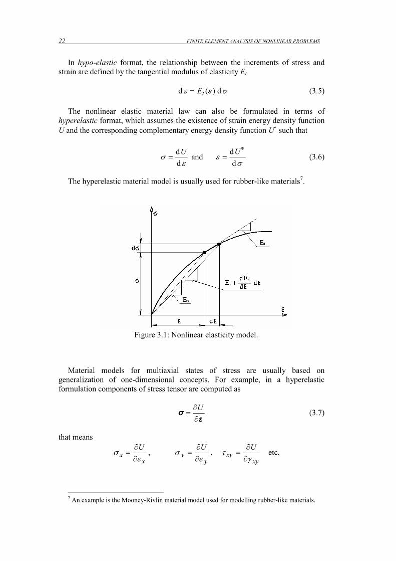
Nonlinear elastic behavior of materials can be formulated in several ways. The simplest is total format, where the stress and strains are defined in terms of the secant modulus of elasticity Es, see Figure 3.1,
εεσ )(sE= (3.4)
22 FINITE ELEMENT ANALYSIS OF NONLINEAR PROBLEMS
In hypo-elastic format, the relationship between the increments of stress and strain are defined by the tangential modulus of elasticity Et
σεε d)(d tE= (3.5)
The nonlinear elastic material law can also be formulated in terms of
hyperelastic format, which assumes the existence of strain energy density function U and the corresponding complementary energy density function U∗ such that
εσ
d
dU= and
σε
d
d ∗=
U (3.6)
The hyperelastic material model is usually used for rubber-like materials7.
Figure 3.1: Nonlinear elasticity model.
Material models for multiaxial states of stress are usually based on
generalization of one-dimensional concepts. For example, in a hyperelastic formulation components of stress tensor are computed as
εσ
∂
∂=
U (3.7)
that means
xx
U
εσ
∂
∂= ,
yy
U
εσ
∂
∂= ,
xyxy
U
γτ
∂
∂= etc.
7 An example is the Mooney-Rivlin material model used for modelling rubber-like materials.

FINITE ELEMENT ANALYSIS OF NONLINEAR PROBLEMS 23
Figure 3.2: Strain energy density functions U and U∗
For any nonlinear elastic material model, it is possible to define relation
between stress and strain increments as
εDσ dd T= (3.8) Matrix DT is function of strains εεεε. Consequently, a set of equilibrium equations
we receive in FEM is nonlinear and must be solved by use of any method (e.g. NR) described above.
3.3 Elastoplastic material model
3.3.1 Yielding criterion
Experiments indicate that linear elastic model is acceptable only within a limited range of stress. As an example, the stress-strain curve from tension test of steel specimen is shown in Figure 3.3. Until the yield stress represented by point A (in the given case σy = 280 MPa) the deformations are elastic and stress-strain relation may be described as σ = E ε. When the stress level exceeds the yield stress, an elastoplastic constitutive law governs the relationship between increments of stress and strain. Due to lack of information,8 approximate stress-strain curves are usually used in analysis. Bilinear approximation defined by yield stress, modulus of elasticity E and tangential modulus ET is shown in Figure 3.4. If ET = 0, material model is elastic-perfectly plastic. If ET ≠ 0 material model assumes strain hardening.
8 In a design process, the real material curve is usually unknown, only basic values like yield
stress etc. are available. Moreover, the material properties slightly differ by different supplies.

24 FINITE ELEMENT ANALYSIS OF NONLINEAR PROBLEMS
0
50
100
150
200
250
300
350
400
450
0.00 0.02 0.04 0.06 0.08 0.10 0.12
εεεε
σσ σσ [
MP
a] A
Figure 3.3: Typical stress-strain curve for mild steel
It should be noted that curves in Figures 3.3 and 3.4 are for tensile behaviour. It
is usually assumed that similar curves for compressive behaviour are applicable if there has been no history of plastic deformation.
Figure 3.4: Elastoplastic model with linear strain hardening
The indication of yielding under multiaxial conditions in metals is obtained
from experiments usually conducted on cylindrical samples subjected to combined axial load and torque. Experiments suggest that there is no significant difference in behaviour of metals in tension or compression and no volume change associated with yielding and no effect of mean stress level on yielding can be assumed.
In a mathematical description, onset of yielding may be represented by a scalar function termed the yield function F. The yield function is written in a form, which leads to the conditions

FINITE ELEMENT ANALYSIS OF NONLINEAR PROBLEMS 25
0<F for elastic and 0=F for plastic deformation. (3.9)
In engineering practice, two following conditions for yielding are most frequently used:
Von Mises yield criterion
02)()()( 213
232
211 =−−+−+−= yF σσσσσσσ (3.10)
where σ1, σ2 and σ3 are principal stresses. Thus, yield occurs when the
effective stress σeff reaches the yield stress value σy
yeff σσσσσσσσ =−+−+−= 213
232
211 )()()(
2
1. (3.11)
Tresca yield criterion
[ ][ ][ ] 0)()()( 2213
2232
2221 =−−−−−−= yyyF σσσσσσσσσ . (3.12)
The largest difference between these two classical yield criteria is about 15%
for the pure shear stress state. For other stress states is the difference less. Hence, both criteria are frequently considered as equivalent in engineering practice.
Any yield condition that is function of stress tensor components σσσσ and material parameters κκκκ
0),( =κσF (3.13)
defines a yield surface in principal stress space, see Figure 3.5. Stress points that lie inside the yield surface are associated with elastic stress states whereas those that lie on the surface represent plastic stress states. No stress point can be outside the yield surface.
Figure 3.5: Yield surface

26 FINITE ELEMENT ANALYSIS OF NONLINEAR PROBLEMS
3.3.2 Post yielding behaviour
The fundamental assumption in describing post-yielding behavior is the decomposition of the total strain increment into an elastic (recoverable) part and a plastic (irreversible) part. For uniaxial stress state is, according to Figure 3.6
TE=εσ
d
d, E
e=
ε
σ
d
d (3.14)
and plastic strain increment is then
σεεε ddddT
Tep
EE
EE −=−= . (3.15)
Figure 3.2: Decomposition of the total strain increment
By analogy, in multiaxial stress state the total strains we decompose into elastic and plastic parts too
peεεε += (3.16)
In multiaxial cases, subsequent loading after first yield produces further plastic
deformation that can result in a modification of the shape and/or position of the yield surface.
For a perfectly plastic material, the yield surface remains unchanged during plastic deformation. For a strain hardening material, plastic deformation produces a change in shape and position of the yield surface. This means that initial yield surface is gradually replaced by the subsequent yield surfaces. A modified yield function is adopted which has a form such as
0),,( =KF pεσ . (3.17)

FINITE ELEMENT ANALYSIS OF NONLINEAR PROBLEMS 27
This yield function depends on the stresses but also the plastic strains and a hardening parameter K. The way in which the plastic strains modify the yield function is defined by hardening rules:
Figure 3.7: Isotropic hardening.
1. An isotropic hardening law implies that the yield surface increases in
size but maintains its original shape under loading conditions. Schematic representation of isotropic hardening for uniaxial and biaxial stress state is shown in Figure 3.7.
2. In kinematic hardening, the original yield surface is translated to a new
position in stress space with no change of its shape and size as shown in Figure 3.8. Kinematic hardening has paramount importance in modelling cyclic behaviour.
3. The combination of the two principal hardening laws leads to a mixed
hardening law, where the initial yield surface both expands and translates as a consequence of plastic flow.
Figure 3.8: Kinematic hardening.

28 FINITE ELEMENT ANALYSIS OF NONLINEAR PROBLEMS
3.3.3 Constitutional equations of elastoplastic material
The yield criterion says whether plastic deformation will occur but says nothing about the plastic behaviour of a material after onset of plastic deformations. This is defined by so-called flow rule in which is the rate and the direction of plastic strains is related to the stress state and the stress rate. This relation can be expressed as
ij
pij
Q
σλε
∂
∂= dd (3.17)
or in matrix form as
σε
∂
∂=
Qp λdd (3.18)
where dλ is a scalar value (to be determined) and Q is a scalar valued function of stress components called plastic potential.
For metals, the so-called associated flow rule, in which the plastic potential surface coincides with the yield surface, i.e.
FQ =
can be adopted to model plastic flow. For some other materials, non-associated flow rule in which FQ ≠ has to be used to model plastic flow adequately. In the following text we will deal with associated flow rule
σε
∂
∂=
Fp λdd (3.19)
Consider a uniaxial stress state first. The plastic behaviour of material is
described as
εσ dd TE= (3.20)
where ET is constant for a bilinear material as obvious from the equations (3.14) and (3.15).
In a multiaxial stress state, we can formulate a similar constitutive equation
εDσ dd T= (3.21)
where tangential material matrix DT can be derived from known stress tensor σσσσ , strain tensor εεεε and from constitutive matrix D from equation (3.1) in following way:
The first step is strain decomposition into elastic dε ε ε ε e and plastic part dε ε ε ε p
peεεε ddd += . (3.22)
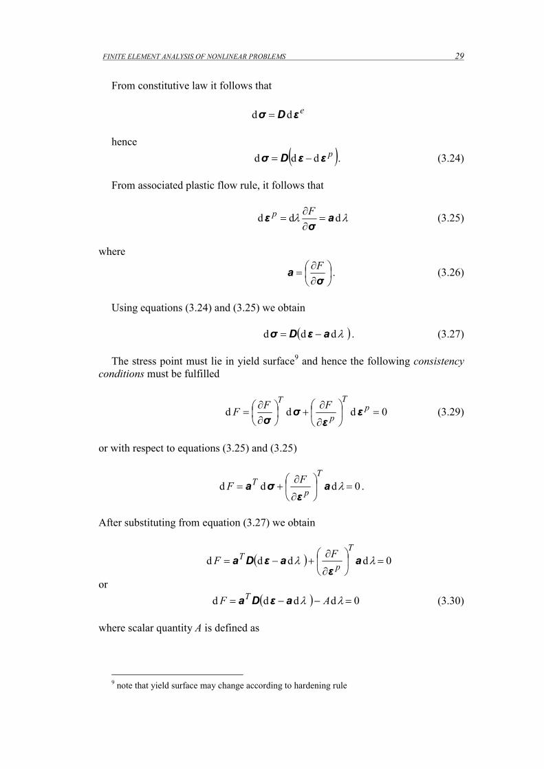
FINITE ELEMENT ANALYSIS OF NONLINEAR PROBLEMS 29
From constitutive law it follows that
eεDσ dd =
hence
( )pεεDσ ddd −= . (3.24) From associated plastic flow rule, it follows that
λλ ddd aσ
ε =∂∂
=Fp (3.25)
where
∂∂
=σ
aF
. (3.26)
Using equations (3.24) and (3.25) we obtain
( )λddd aεDσ −= . (3.27)
The stress point must lie in yield surface9 and hence the following consistency
conditions must be fulfilled
0ddd =
∂
∂+
∂∂
= pT
p
TFF
F ε
ε
σσ
(3.29)
or with respect to equations (3.25) and (3.25)
0ddd =
∂
∂+= λa
ε
σa
T
p
T FF .
After substituting from equation (3.27) we obtain
( ) 0dddd =
∂
∂+−= λλ a
ε
aεDa
T
p
T FF
or
( ) 0dddd =−−= λλ AF TaεDa (3.30)
where scalar quantity A is defined as
9 note that yield surface may change according to hardening rule

30 FINITE ELEMENT ANALYSIS OF NONLINEAR PROBLEMS
a
ε
T
p
FA
∂
∂−= . (3.31)
Now, we can derive parameter dλ from equation (3.29)
aDa
εDa
T
T
A+=
ddλ (3.32)
and substituting this expression for dλ into equation (3.28) we finally obtain
ε
aDa
DaaDDσ dd
+−=
T
T
A. (3.33)
When compare the last equation with equation (3.21) we can see that
aDa
DaaDDD
T
T
TA+
−= . (3.34)
Note that material matrix D is symmetric, i.e. DD =T , hence matrix DT is symmetric as well. 3.3.4 Integration of constitutive equations
We have derived that for infinitesimal increments of stress and strain it holds
εDσ dd T= .
In FE analysis we need to work with finite increments σ∆ and ε∆ for which is the relation above approximate only, so if we use relation
εDσ ∆=∆ T for large increments of stress and strain, an error occurs as stress σσ ∆+ in subsequent step will not satisfy constitutive law and consistency condition. Hence, we need to integrate over the increment of pseudo-time
∫∆
=∆t
σσ d
where, according to equation (3.24)
( )pεεDσ ddd −= .

FINITE ELEMENT ANALYSIS OF NONLINEAR PROBLEMS 31
It is important to note that if plastic flow is present, the TD changes during increment t∆ and as a result, the ratio between total and plastic strain changes too.
To obtain correct results, various stress increment integration schemes that differs in the degree of approximation have been developed. Frequently used are the following schemes:
3.3.4.1 Generalised trapezoidal rule
Consider that we know stress nσ , total strain nε and plastic strain pnε at time
step n. Then at step n+1
( )pnnnnnn 1111 ++++ ∆−∆+=∆+= εεDσσσσ (3.35)
( )[ ]11 1 ++ +−∆=∆ nnpn aaε ααλ (3.36)
01 =+nF (3.37)
3.3.4.2 Generalised mid point rule
( )pnnnnnn 1111 ++++ ∆−∆+=∆+= εεDσσσσ (3.35)
αλ ++ ∆=∆ npn aε 1 (3.36)
0=+αnF (3.37)
In both rules, α is a parameter ranging from 0 to 1. For 0=α we obtain explicit
forward Euler integration scheme. Advantage of this algorithm is in its simplicity; disadvantage is that it is conditionally stable only. That means that step increment has to be smaller than some critical value to avoid instability of the solution.
For 1=α we obtain implicit backward Euler integration scheme
( )pnnn 111 +++ ∆−∆=∆ εεDσ
11 ++ ∆=∆ npn aε λ
( ) 0, 111 == +++ nnn FF εσ
It is obvious that in difference with forward scheme, we deal with values defined at the end of the increment, which are unknown at start of it. Hence, the procedure is of an iterative nature. This means that at beginning of the increment, the trial stress is estimated by assuming elastic deformation and computed values are then checked whether consistency condition and constitutional equation are satisfied. If not, the process is repeated with improved values until the conditions are satysfied.

32 FINITE ELEMENT ANALYSIS OF NONLINEAR PROBLEMS
3.3.5 Numerical procedures
The tangential material matrix DT is used to form a tangential stiffness matrix KT. When the tangential stiffness matrix is defined, the displacement increment is obtained for a known load increment
FdK ∆=∆T (3.22)
As load and displacement increments are final, not infinitesimal, displacements
obtained by solution of this set of linear algebraic equation will be approximate only. That means, conditions of equilibrium of internal and external nodal forces will not be satisfied and iterative process is necessary. Any of methods mentioned above may be used.
The problem that arises now is the fundamental problem in computational elastoplasticity - not only equilibrium equations but also constitutive equations of material must be satisfied. That means that within the each equilibrium iteration step check of stress state and iterations to find elastic and plastic part of strains at every integration point must be included. The iteration process continues until both, equilibrium conditions and constitutive equations are satisfied simultaneously. The converged solution at the end of load increment is then used at the start of new load increment.

FINITE ELEMENT ANALYSIS OF NONLINEAR PROBLEMS 33
REFERENCES
[1] Hinton, E: Introduction to Nonlinear Finite Element Analysis. NAFEMS, Glasgow 1992
[2] Crisfield, M. A.: Non-linear Finite Element Analysis of Solids and Structures. John Wiley & Sons 1991
[3] Bittnar, Z., Šejnoha, J.: Numerické metody mechaniky (Numerical methods of mechanics). ČVUT, Praha 1992
[4] Okrouhlík, M., Höshl, C., Plešek, J., Pták, S., Nadrchal, J.: Mechanika poddajných těles, numerická matematika a superpočítače (Mechanic of solids, numerical mathematics and supercomputers). Czech Academy of Science, Prague 1997.
[5] Okrouhlík, M.: Implementation of Nonlinear Continuum Mechanics in Finite Element Codes. Institute of Thermodynamics, Prague 1995.
[6] Hinton, E., Ezatt, M., H.: Fundamental Tests for Two and Three Dimensional, Small Strain, Elastoplastic Finite Element Analysis. NAFEMS, Glasgow 1987.
[7] Electronic documentation of program COSMOS/M, version 2.95. SRAC, Los Angeles 2005, www,cosmosm.com.
[8] Falzon, B., G., Hitchings, D.: An Introduction to Modeling Buckling and Collapse. NAFEMS, Glasgow 2006
[9] Eurocode 3: Design of steel structures - Part 1-1: General rules and rules for buildings. CEN, Brussels 2005.
34 FINITE ELEMENT ANALYSIS OF NONLINEAR PROBLEMS
APPENDIX

FINITE ELEMENT ANALYSIS OF NONLINEAR PROBLEMS 35
NONLINEAR ANALYSES WITH COSMOS/M
PROGRAM
1.1 Properties of finite elements
For nonlinear analyses it is necessary to compute tangential stiffness matrices of individual elements. This possibility is available only for some elements according to Table 1.
Table 1: Properties of finite elements
Material model Element Name
Element Description GNL Le Ne Pl Ve He
TRUSS2D Plane truss • • • • • TRUSS3D Space truss • • • • • BEAM2D Plane beam • • • • • BEAM3D Space beam • • • • • SPRING Axial an/or torsional spring • • •
PLANE2D 4 to 8 node plane stress, plane strain, axisymmetric element • • • • • •
TRIANG 3 to 6 node plane stress, plane strain, axisymmetric triangular element
• • • • • •
SHELL3 3-node triangular thin shell • • • • • • SHELL4 4-node quadrilateral thin shell • • • • • • SHELL3T 3-node triangular thick shell • • • • • • SHELL6 6-node triangular thin shell • SHELL6 6-node triangular thick shell • SHELL4T 4-node quadrilateral thick shell • • • • • • SHELL3L 3-node triangular composite shell • •
SHELL4L 4-node quadrilateral composite shell • •
SOLID 8 to 20 node hexahedron • • • • • • TETRA4 4-node tetrahedron • • • • • • TETRA10 10-node tetrahedron • • • • • • GAP Contact element with friction MASS Concentrated mass
GNL Geometric nonlinearities Le Linear elastic material Ne Nonlinearly elastic material Pl Elastic-plastic material Ve Viscoelastic material He Hyper elastic material

36 FINITE ELEMENT ANALYSIS OF NONLINEAR PROBLEMS
Nonlinear properties of individual elements should be defined in element
options. For example, steps needed for specification of SOLID element properties are shown in Figure 4 and subsequent figures.
Figure 4: Definition of finite element group
Figure 5: Element specification
Figure 6: Option 1 of the SOLID element

FINITE ELEMENT ANALYSIS OF NONLINEAR PROBLEMS 37
Figure 7: Definition of material model
Figure 8: Definition of geometric nonlinearity

38 FINITE ELEMENT ANALYSIS OF NONLINEAR PROBLEMS
Figure 9: Listing of element groups – element group 1 defines a linear element SOLID; element group 2 defines geometric and material nonlinear element.
1.2 Nonlinear analysis setup
Parameters of nonlinear analysis are specified from MENU ANALYSIS / NONLINEAR, see Figure 10. Individual items in this menu have following use:
1. Solution Control – definition of method of solution of system of nonlinear equations. Possible values are in Figure 11.
2. Integration Options – definition of method of solution for dynamic problems, see Figure 12.
3. Auto Step Option – if is set “ON”, the program automatically selects optimal size of time increments according to convergence in previous time steps, see Figure 13.
4. Base Motion Parameter and Damping Coefficient – applicable for dynamic problems only.
5. Print Options – specification what will be written in output file name of problem.OUT. The advisable is to oppress printing of large files that are difficult to read. Recommended is to use setup according to Figure 14.
6. Plot Options – specification for which steps will program store results. Normally, if nothing is specified, results are stored for the last successfully accomplished step only. If there is need to store more results to plot and list, these steps have to be specified as shown Figure 15.

FINITE ELEMENT ANALYSIS OF NONLINEAR PROBLEMS 39
7. Response Options – specification for which nodes will program store results to plot nodal values as displacements and reactions, see Figure 16. This specification is useful if we do not need results for all nodes. If a plot option is specified for all steps, this option is not necessary.
Figure 10: Nonlinear Analysis Menu

40 FINITE ELEMENT ANALYSIS OF NONLINEAR PROBLEMS
Figure 11: Solution Control menu
Figure 12: Integration method for solution of dynamic problems specification
Figure 13: Auto step definition – minimum acceptable time increment is set to
10-6, maximum allowed time increment is 1,5 and maximum number of trials to select proper time increment is limited to 5.

FINITE ELEMENT ANALYSIS OF NONLINEAR PROBLEMS 41
Figure 14: Output file specification
Figure 15: Specification that results will be stored for steps 1, 2, 3, 4, 5, 6, 7, 8,
9, 10 and then for steps 12, 14, 16, 18 and 20

42 FINITE ELEMENT ANALYSIS OF NONLINEAR PROBLEMS
Figure 16: Specification of nodes to plot graphs
8. Nonlinear Analysis Options – detailed specification of analysis. Default setup, which is appropriate for most nonlinear static problems is in Figure 17.
9. Run Nonlinear Analysis – start of computations. For other items of the NONLINEAR menu refer to the program COSMOS/M
documentation.

FINITE ELEMENT ANALYSIS OF NONLINEAR PROBLEMS 43
Figure 17: Specification of nonlinear analysis – default values of parameters

44 FINITE ELEMENT ANALYSIS OF NONLINEAR PROBLEMS
1.3 Time curves and time parameters
At least one time curve has to be specified for nonlinear analysis. Time curves can be defined from menu Loads BC , see Figure 18 and subsequent figures.
or from icons in left panel
Figure 18: Start of definition of time curves
Figure 19: Time curve definition – 1st step

FINITE ELEMENT ANALYSIS OF NONLINEAR PROBLEMS 45
Figure 20: Time curve definition – 2nd step (in this example, definition of the
time curve number 1 is prepared)
Figure 21: Time curve definition – 3rd step –coordinates of points will start with
first point 10
Figure 22: Definition of points of the time curve
10 start point number higher than 1 we use in a case that curve is defined and we want to add
some points

46 FINITE ELEMENT ANALYSIS OF NONLINEAR PROBLEMS
To plot a time curve, commands from menu DISPLAY can be selected as
shown in figure and subsequent figures.
Figure 23: Commands to prepare a plot of a time curve

FINITE ELEMENT ANALYSIS OF NONLINEAR PROBLEMS 47
Figure 24: Commands to plot a time curve
Figure 25: Graph of the time curve number 1 as defined in Figure 22

48 FINITE ELEMENT ANALYSIS OF NONLINEAR PROBLEMS
Note that after definition, the time curve became active. This means that
boundary conditions defined subsequently will be associated with it. To deactivate a time curve or to switch activation to another one, the commands according to Figure 26 should be used.
Figure 26: Making a time curve active (or not active)

FINITE ELEMENT ANALYSIS OF NONLINEAR PROBLEMS 49
1.4 Restart possibilities
Nonlinear analyses are time demanding. This is a reason that there is a possibility to continue in computation after stop of program. For this so called restart of computation the parameter RESTART, see Figure 27 have to be set to 1. If set to 0, computation will start from beginning.
Figure 27: Restart options

50 FINITE ELEMENT ANALYSIS OF NONLINEAR PROBLEMS
EXAMPLES OF COSMOS/M PROGRAM USE
1.5 Compressed slender beam
Problem description: Slender elastic beam is compressed by force F and laterally loaded by a small force P. The forces increase according to time curves11 TC 1 and TC 2. Force P = 200 N is associated with the curve TC 1 and force F = 100000 N with the curve TC 212. Dimensions of the beam are L = 1600 mm, a = 80 mm and t = 3 mm. Modulus of elasticity is E = 2,1⋅105 MPa.
Fig. 1: Compressed beam
0
0.2
0.4
0.6
0.8
1
1.2
1.4
1.6
1.8
0 0.2 0.4 0.6 0.8 1 1.2 1.4 1.6 1.8 2
TC 1
TC 2
Fig. 2: Time curves
11 The time is now only a parameter controlling the loading, because the problem is static. 12 Association with a time curve means that at every time the value of force is multiplied by
instantaneous value of time curve ordinate.

FINITE ELEMENT ANALYSIS OF NONLINEAR PROBLEMS 51
Modelling hints:
1. The BEAM2D element group is used to model beam. As the problem is geometrically non-linear, finer finite element mesh must be used than for a linear problem. Geometric nonlinearities are taken into account if option 6 for the element group BEAM2D is set to 1 (large displacement formulation).
2. It is useful to perform linear and buckling analyses before the nonlinear
analysis. For comparison, the Euler critical force is given by 2
2
)2( L
IEF zcr
π= .
For the dimensions and modulus of elasticity given above is Fcr = 185088,7 N.
3. Load should be divided into small increments and NR, or MNR iterations of equilibrium should be used for each incremental step.
4. Finer load increments are necessary when F → Fcr.
5. Restart from the last successfully accomplished load increment can be performed.
Commands:
C* 1. Geometry creation VIEW,0,0,1,0 PT,1,0,0,0 CREXTR,1,1,1,Y,1600 CREXTR,2,2,1,Y,1600 C* 2. Defining material properties MPROP,1,EX,2.1E5 C* 3. Defining elemnt group and beam section EGROUP,1,BEAM2D,0,0,0,0,0,1,0,0 BMSECDEF,1,1,4,1,9,80,80,3,3,0,0,0,0,0 C* 4. Creating FE mesh M_CR,1,2,1,2,5,1 NMERGE,1,12,1,1,0,0,0 NCOMPRESS,1,12 C* 5. Defining boundary conditions C* 5.1 prescribed displacements DPT,1,UX,0,3,2, DPT,1,UY,0,1,1, C* 5.2 defining force P CURDEF,TIME,1,1,0,0,.1,1,10,1 FPT,2,FX,200,2,1 C* 5.3 force F CURDEF,TIME,2,1,0,0,10,10,10 FPT,3,FY,-1E5,3,1 C* 6. Adjusting nonlinear analysis A_NONLINEAR,S,1,1,20,0.001,0,N,0,0,1E+010,0.001,0.01,0,1,0,0 NL_PLOT,1,100,1,0 C* 7. specification of load increments TIMES,0,1.7,.1 C* 7. nonlinear analysis

52 FINITE ELEMENT ANALYSIS OF NONLINEAR PROBLEMS
R_NONLIN C* restart from the last step RESTART,1 TIMES,1.7,1.8,0.02 R_NONLIN C* RESTART,1 TIMES,1.8,1.82,0.005 R_NONLIN
Results: Typical nonlinear response is obvious from the graph (Figure 3)
showing beam deflection at the middle of span versus load parameter (time).
0
5
10
15
20
25
0 0,2 0,4 0,6 0,8 1 1,2 1,4 1,6 1,8 2
TIME
UX
[m
m]
Fig. 3: Deflection versus time

FINITE ELEMENT ANALYSIS OF NONLINEAR PROBLEMS 53
1.6 Thick-walled pipe subjected to internal pressure
Problem description: The long cylindrical pressure vessel is subjected to internal pressure. Both ends are assumed fixed. Compute stress distribution during pressure test and during normal operation. Assume small plastic deformations according to bilinear material model if yield stress is σY = 260 MPa, modulus of elasticity is E = 2,1.105 MPa and tangent modulus is ET = 100 MPa.
Fig. 4: Thick walled pipe
0
50
100
150
200
250
300
0 0.005 0.01 0.015 0.02 0.025 0.03
strain
str
ess
Fig. 5: Bilinear material mode
Time curve reflects load history. During test is internal pressure increased to
1,2 × nominal value, which is 120 MPa.

54 FINITE ELEMENT ANALYSIS OF NONLINEAR PROBLEMS
Fig. 6: Load history – time curve
Modelling hints:
1. Due to axial symmetry, only a part of the cylinder longitudinal section may be modelled.
2. 8 node PLANE2D elements are used with option 5 set to “Von Mises kinematic hardening”.
3. Load incrementation with NR iterations should be used. 4. Restart is used to change load (time) increment.
Fig. 7: FE mesh and boundary conditions
Commands:
C* GEOMETRY CREATION VIEW,0,0,1,0 PT,1,45,0,0 CREXTR,1,1,1,X,35 SFEXTR,1,1,1,Y,10 C* DEFINING ELEMENT GROUP EGROUP,1,PLANE2D,0,2,1,0,2,0,0,0 C* DEFINING MATERIAL PROPERTIES

FINITE ELEMENT ANALYSIS OF NONLINEAR PROBLEMS 55
MPROP,1,EX,2.1E5 MPROP,1,NUXY,.3 MPROP,1,ETAN,100 MPROP,1,SIGYLD,260 C* MESHING M_SF,1,1,1,8,8,2,1,1 C* DEFINING BOUNDARY CONDITIONS DCR,2,UY,0,1,1, CURDEF,TIME,1,1,0,0,1,1.2,1.1,1.2,2,0,3,1 PCR,3,120,3,1,120,4 C* ADJUSTING NONLINEAR ANALYSIS NL_CONTROL,0,1 NL_PRINT,0,0,0,0,0,0,0 NL_PLOT,1,50,1,0 C* TEST SIMULATON TIMES,0,1,.2 R_NONLIN C* RESTART,1 TIMES,1,1.1,.1 R_NONLIN C* UNLOADING TIMES,1.1,2,0.09 R_NONLIN C* C* NOMINAL PRESSURE LOADING TIMES,2,3,0.2 R_NONLIN C*
Results: Note that
1. Linear analysis gives non-realistic values of stress (maximal von Mises stress is about 304 MPa).
2. Plastic deformations occur during test loading.
3. After test, residual stress is present in the cylinder. This redistribution of stress is useful and desired.
4. Due to stress redistribution, only stress within elastic range is present during nominal loading after the test.

56 FINITE ELEMENT ANALYSIS OF NONLINEAR PROBLEMS
1.7 Deformation of a thin-walled tank
Problem description: Thin-walled pressure vessel – tank is subjected to internal pressure. Compute stress distribution according to linear and nonlinear static analysis. In the nonlinear analysis, both geometrical and material nonlinearities should be taken into account. Material is elastoplastic, the same as in previous example (Figure 5). Nominal value of internal pressure is 0,6 MPa. Symmetric half of the tank is shown in Figure 8. Diameter of the manhole cover (thickness of 25 mm) is 600 mm.
Fig. 8: Thin-walled tank
Modelling hints:
1. SHELL4T elements with options for large displacement, small plastic strain, von Mises yield criterion and kinematic hardening are used.
2. Due to symmetry, only one eighth of the tank may be modelled. 3. Stresses are calculated in element co-ordinate systems. To receive compatible
co-ordinate systems curves are reoriented. 4. Element co-ordinate system of SHELL4T element is defined according to
Figure 9. The element x-axis goes from the first node to the second. The y-axis lies in the plane defined by the first three nodes perpendicular to the x-axis toward the fourth node. The z-axis completes a right-hand Cartesian system. When meshing surfaces, element x-axes are parallel to the first surface curve marked by asterisks in Figure 10. FE mesh is shown in Figure 11.
5. The automatic time stepping and restart options are used for nonlinear FE analysis.

FINITE ELEMENT ANALYSIS OF NONLINEAR PROBLEMS 57
Figure 9: Element co-ordinate system (ECS).
1
2
4
3 x
y
z TOP FACE
BOTTOM FACE
Fig. 9: Element co-ordinate system (ECS)
Fig. 10: Orientation of shell elements
Fig. 11: Finite element mesh

58 FINITE ELEMENT ANALYSIS OF NONLINEAR PROBLEMS
Figure 28: Example of inappropriate orientation of elements – orientation of
elements on surface 1 differs from orientation of other elements13
Figure 29: Orientation of surfaces identification
13 top faces of shell elements are red colour, bottom faces are blue

FINITE ELEMENT ANALYSIS OF NONLINEAR PROBLEMS 59
Commands:
C*
C* 1. DEFINING GEOMETRY
C* C* 1.1. creating points and curves C* VIEW,0,0,1,0 PT,1,0,0,0 PT,2,2900,0,0 PLANE,Z,0,1 CRPCIRCLE,1,2,1,2900,-80,1 PT,4,0,1700,0 C* CREXTR,4,4,1,X,2450 C* 1.1.1 intersecting curves CRINTCC,1,2,2,1,2,5E-005 C* 1.1.2 deleting useless curves CRDEL,4,2,2 C* 1.1.3 creating fillet etc. CRFILLET,4,1,3,400,1,0,1E-006 PT,10,-20,300,0 CREXTR,10,10,1,X,100 CRINTCC,1,5,5,1,0,5E-005 CRDEL,1,1,1 CRDEL,5,5,1 CREXTR,12,12,1,Y,-300 C* 1.1.4 changing orientation of curves 3 and 7 in order to receive
desired C* ECS orientation CRREPAR,7,3,4 VIEW,-1,2,3,0 CRCOMPRESS,1,7 C* C* 1.2 creating surfaces C* SFSWEEP,1,4,1,X,90,2 C*
C* 2. FE MESH DEFINITION
C* 2.1 defining element type and real constant sets EGROUP,1,SHELL4T,1,0,0,1,2,1,0,0 RCONST,1,1,1,6,6,0,0,0,0,0 RCONST,1,2,1,6,25,0,0,0,0,0 C* 2.2 defining material properties MPROP,1,EX,2.1E5,NUXY,.3,SIGYLD,260 MPROP,1,ETAN,100 C* 2.3 meshing ACTSET,RC,1 M_SF,5,6,1,4,10,6,1.8,1 VIEW,-1.5,2,2,0 ACTSET,RC,2 MA_NUSF,7,8,1,4,4,6,0 MASFCH,7,8,1,Q,4,1,0.4,1

60 FINITE ELEMENT ANALYSIS OF NONLINEAR PROBLEMS
ACTSET,RC,1 M_SF,3,4,1,4,3,6,1,1 M_SF,1,2,1,4,10,6,2,1 NMERGE,1,400,1,1,0,0,0 NCOMPRESS,1,400 NCOMPRESS,1,330 ECOMPRESS,1,315 C* 2.4 checking real constants assignment ACTECLR,1,RC,1 SHADE,1,4,1 EPLOT,1,ELMAX,1 ACTECLR,0 C* C* 3. DEFINING BOUNDARY CONDITIONS C* C* 3.1 displacements SELPIC,CR,20,16,12,6,0 DCR,1,SY,0,CRMAX,1, INITSEL,CR,1,1 SELPIC,CR,4,3,2,1,0 DCR,1,SZ,0,CRMAX,1, INITSEL,ALL,1,1 DCR,8,SX,0,10,2, CLS,1 C* 3.2 pressure CURDEF,TIME,1,1,0,0,10,10 PSF,1,0.6,8,1,0.6,0.6,4 C* C* 4. ANALYSIS C* 4.1 preliminary linear static analysis C* R_STAT C* C* 4.2 nonlinear analysis adjustment NL_AUTOSTEP,1,.001,.1,5 NL_PLOT,1,20,1,0 NL_PRINT,0,0,0,0,0,0,0 A_NONLINEAR,S,1,1,20,0.001,0,N,0,1,1E+010,0.001,0.01,0,1,0,0 C* 4.3 running nonlinear analysis TIMES,0,1,.1 R_NONLIN C* C* 4.4 continuing in NL analysis RESTART,1 TIMES,1,1.5,.1 R_NONLIN C* C* 5. POSTPROCESSING C* plotting stress, displacements and xy graphs. C*

FINITE ELEMENT ANALYSIS OF NONLINEAR PROBLEMS 61
Results:
1. Von Mises stress distribution for time step 16 (t = 1,5) on top faces of shell
elements is in . Von Mises stress distribution on bottom faces is in . 2. There are large differences between results of linear and nonlinear analysis. In
linear analysis the von Mises stress is above the yield stress 260 MPa. Difference between linear and nonlinear analysis results is a consequence of different solution methods. While in the linear analysis is stress considered as elastic and geometry of the tank is considered unchanged, in the nonlinear analysis changes of the tank shape are taken into account together with material nonlinearities.
3. Onset of plastic deformation is obvious from the graph in Fig. 12.
Figure 30: Von Mises stress distribution on top faces at t = 1,5.

62 FINITE ELEMENT ANALYSIS OF NONLINEAR PROBLEMS
Figure 31: Von Mises stress distribution on bottom faces at t = 1,5.
0
40
80
120
160
200
240
280
0 0.3 0.6 0.9 1.2 1.5
time
σ [
MP
a]
Fig. 12: Course of equivalent von Mises stress in node 177