Faunus Provides Big Graph Data Analytics

NOVEMBER 11, 2012 1 COMMENT

Faunus is an Apache 2 licensed distributed graph analytics engine

that is optimized for batch processing graphs represented across a multi-machine

cluster. Faunus makes global graph scans efficient because it leverages sequential

disk reads/writes in concert with various on-disk compression techniques. Moreover,

for non-enumerative calculations, Faunus is able to linearly scale in the face

of combinatorial explosions. To substantiate these aforementioned claims, this post

presents a series of analyses using a graph representation of Wikipedia (as provided

by DBpedia version 3.7). The DBpedia knowledge graph is stored in a

7 m1.xlargeTitan/HBase Amazon EC2 cluster and then batch processed using

Faunus/Hadoop. Within the Aurelius Graph Cluster, Faunus provides Big Graph Data

analytics.

Ingesting DBpedia into Titan

The DBpedia knowledge base currently describes 3.77 million things, out of which 2.35

million are classified in a consistent Ontology, including 764,000 persons, 573,000

places (including 387,000 populated places), 333,000 creative works (including

112,000 music albums, 72,000 films and 18,000 video games), 192,000 organizations

(including 45,000 companies and 42,000 educational institutions), 202,000 species and

5,500 diseases. (via DBpedia.org)

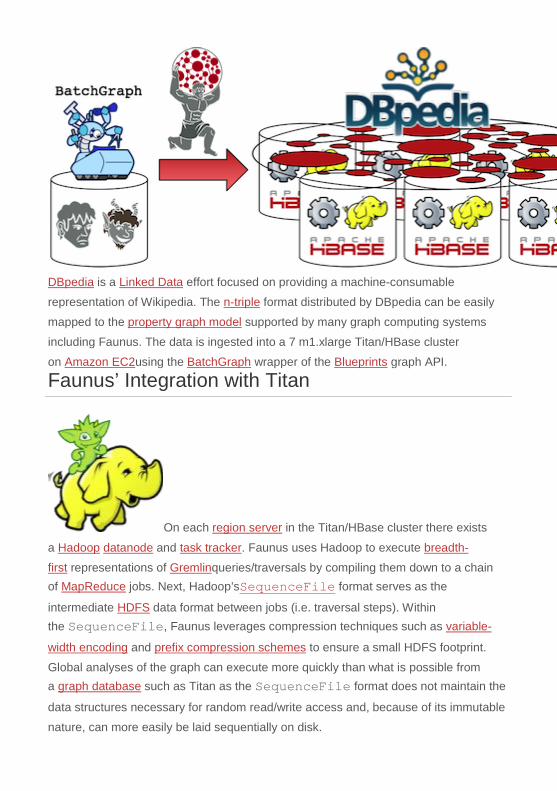
DBpedia is a Linked Data effort focused on providing a machine-consumable

representation of Wikipedia. The n-triple format distributed by DBpedia can be easily

mapped to the property graph model supported by many graph computing systems

including Faunus. The data is ingested into a 7 m1.xlarge Titan/HBase cluster

on Amazon EC2using the BatchGraph wrapper of the Blueprints graph API.

Faunus’ Integration with Titan

On each region server in the Titan/HBase cluster there exists

a Hadoop datanode and task tracker. Faunus uses Hadoop to execute breadth-

first representations of Gremlinqueries/traversals by compiling them down to a chain of MapReduce jobs. Next, Hadoop’sSequenceFile format serves as the

intermediate HDFS data format between jobs (i.e. traversal steps). Within the SequenceFile, Faunus leverages compression techniques such as variable-

width encoding and prefix compression schemes to ensure a small HDFS footprint.

Global analyses of the graph can execute more quickly than what is possible from a graph database such as Titan as the SequenceFile format does not maintain the

data structures necessary for random read/write access and, because of its immutable

nature, can more easily be laid sequentially on disk.

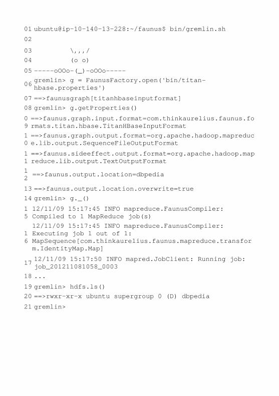
01 ubuntu@ip-10-140-13-228:~/faunus$ bin/gremlin.sh 02 03 \,,,/ 04 (o o) 05 -----oOOo-(_)-oOOo-----

06 gremlin> g = FaunusFactory.open('bin/titan-hbase.properties') 07 ==>faunusgraph[titanhbaseinputformat] 08 gremlin> g.getProperties() 09 ==>faunus.graph.input.format=com.thinkaurelius.faunus.formats.titan.hbase.TitanHBaseInputFormat

10 ==>faunus.graph.output.format=org.apache.hadoop.mapreduce.lib.output.SequenceFileOutputFormat

11 ==>faunus.sideeffect.output.format=org.apache.hadoop.mapreduce.lib.output.TextOutputFormat

12 ==>faunus.output.location=dbpedia

13 ==>faunus.output.location.overwrite=true 14 gremlin> g._() 15

12/11/09 15:17:45 INFO mapreduce.FaunusCompiler: Compiled to 1 MapReduce job(s)

16

12/11/09 15:17:45 INFO mapreduce.FaunusCompiler: Executing job 1 out of 1: MapSequence[com.thinkaurelius.faunus.mapreduce.transform.IdentityMap.Map]

17 12/11/09 15:17:50 INFO mapred.JobClient: Running job: job_201211081058_0003 18 ... 19 gremlin> hdfs.ls() 20 ==>rwxr-xr-x ubuntu supergroup 0 (D) dbpedia 21 gremlin>

The

first step to any repeated analyses of a graph using Faunus is to pull the requisite data

from a source location. For the examples in this post, the graph source is Titan/HBase.

In the code snippet above, the identity function is evaluated which simply maps the Titan/HBase representation of DBpedia over to an HDFS SequenceFile (g._()).

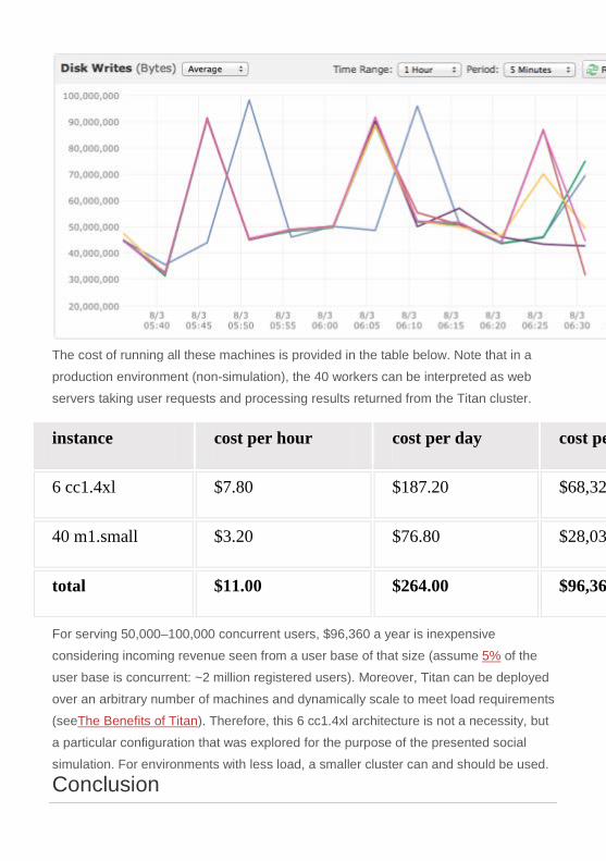
This process takes approximately 16 minutes. The chart below presents the average

number of bytes per minute written to and from the cluster’s disks during two distinct

phases of processing.

1. On the left is the ingestion of the raw DBpedia data into Titan via BatchGraph. Numerous low-volume writes occur over a long period of

time.

2. On the right is Faunus’ mapping of the Titan DBpedia graph to a SequenceFile in HDFS. Fewer high volume reads/writes occur over a

shorter period of time.

The plot reiterates the known result that sequential reads from disk are nearly 1.5x

faster than random reads from memory and 4-5 orders of magnitude faster than

random reads from disk (see The Pathologies of Big Data). Faunus capitalizes on

these features of the memory hierarchy so as to ensure rapid full graph scans.

Faunus’ Dataflows within HDFS: Graph and SideEffect

Faunus has two parallel data flows: graph and sideeffect. Each MapReduce job reads the graph, mutates it in some way, and then writes it back to HDFS as graph* (or to

its ultimate sink location). The most prevalent mutation to graph* is the propagation

of traversers (i.e. the state of the computation). The graph SequenceFile encodes

not only the graph data, but also computational metadata such as which traversers are

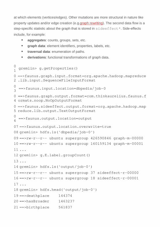
at which elements (vertices/edges). Other mutations are more structural in nature like

property updates and/or edge creation (e.g.graph rewriting). The second data flow is a step-specific statistic about the graph that is stored in sideeffect*. Side-effects

include, for example: aggregates: counts, groups, sets, etc.

graph data: element identifiers, properties, labels, etc.

traversal data: enumeration of paths.

derivations: functional transformations of graph data.

01 gremlin> g.getProperties()

02 ==>faunus.graph.input.format=org.apache.hadoop.mapreduce.lib.input.SequenceFileInputFormat

03 ==>faunus.input.location=dbpedia/job-0

04 ==>faunus.graph.output.format=com.thinkaurelius.faunus.formats.noop.NoOpOutputFormat

05 ==>faunus.sideeffect.output.format=org.apache.hadoop.mapreduce.lib.output.TextOutputFormat

06 ==>faunus.output.location=output

07 ==>faunus.output.location.overwrite=true 08 gremlin> hdfs.ls('dbpedia/job-0') 09 ==>rw-r--r-- ubuntu supergroup 426590846 graph-m-00000 10 ==>rw-r--r-- ubuntu supergroup 160159134 graph-m-00001 11 ... 12 gremlin> g.E.label.groupCount() 13 ... 14 gremlin> hdfs.ls('output/job-0') 15 ==>rw-r--r-- ubuntu supergroup 37 sideeffect-r-00000 16 ==>rw-r--r-- ubuntu supergroup 18 sideeffect-r-00001 17 ... 18 gremlin> hdfs.head('output/job-0') 19 ==>deathplace 144374 20 ==>hasBroader 1463237 21 ==>birthplace 561837

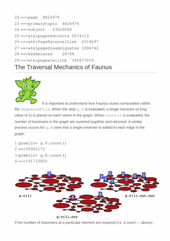
22 ==>page 8824974 23 ==>primarytopic 8824974 24 ==>subject 13610094 25 ==>wikipageredirects 5074113 26 ==>wikiPageExternalLink 6319697 27 ==>wikipagedisambiguates 1004742 28 ==>hasRelated 28748 29 ==>wikipagewikilink 145877010 The Traversal Mechanics of Faunus

It is important to understand how Faunus stores computation within the SequenceFile. When the step g.V is evaluated, a single traverser (a long

value of 1) is placed on each vertex in the graph. When count() is evaluated, the

number of traversers in the graph are summed together and returned. A similar process occurs for g.E save that a single traverser is added to each edge in the

graph.

1 gremlin> g.V.count() 2 ==>30962172 3 gremlin> g.E.count() 4 ==>191733800

If the number of traversers at a particular element are required (i.e. a count — above)

as oppposed to the specific traverser instances themselves (and their respective path

histories — below), then the time it takes to compute acombinatorial computation can

scale linearly with the number of MapReduce iterations. The Faunus/Gremlin traversals

below count (not enumerate) the number of 0-, 1-, 2-, 3-, 4-, and 5-step paths in the

DBpedia graph. Note that the runtimes scale linearly at approximately 15 minutes per

traversal step even though the results compound exponentially such that, in the last

example, it is determined that there are 251 quadrillion length 5 paths in the DBpedia

graph.

01 gremlin> g.V.count() // 2.5 minutes 02 ==>30962172 03 gremlin> g.V.out.count() // 17 minutes 04 ==>191733800 05 gremlin> g.V.out.out.count() // 35 minutes 06 ==>27327666320 07 gremlin> g.V.out.out.out.count() // 50 minutes 08 ==>5429258407462 09 gremlin> g.V.out.out.out.out.count() // 70 minutes 10 ==>1148261617434916 11 gremlin> g.V.out.out.out.out.out.count() // 85 minutes 12 ==>251818304970074185

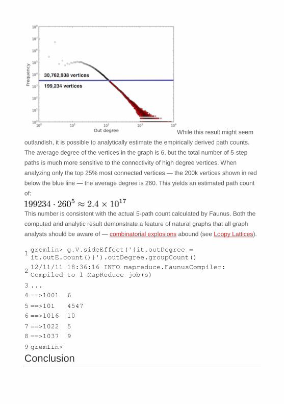
While this result might seem

outlandish, it is possible to analytically estimate the empirically derived path counts.

The average degree of the vertices in the graph is 6, but the total number of 5-step

paths is much more sensitive to the connectivity of high degree vertices. When

analyzing only the top 25% most connected vertices — the 200k vertices shown in red

below the blue line — the average degree is 260. This yields an estimated path count

of:

This number is consistent with the actual 5-path count calculated by Faunus. Both the

computed and analytic result demonstrate a feature of natural graphs that all graph

analysts should be aware of — combinatorial explosions abound (see Loopy Lattices).

1 gremlin> g.V.sideEffect('{it.outDegree = it.outE.count()}').outDegree.groupCount()

2 12/11/11 18:36:16 INFO mapreduce.FaunusCompiler: Compiled to 1 MapReduce job(s) 3 ... 4 ==>1001 6 5 ==>101 4547 6 ==>1016 10 7 ==>1022 5 8 ==>1037 9 9 gremlin> Conclusion

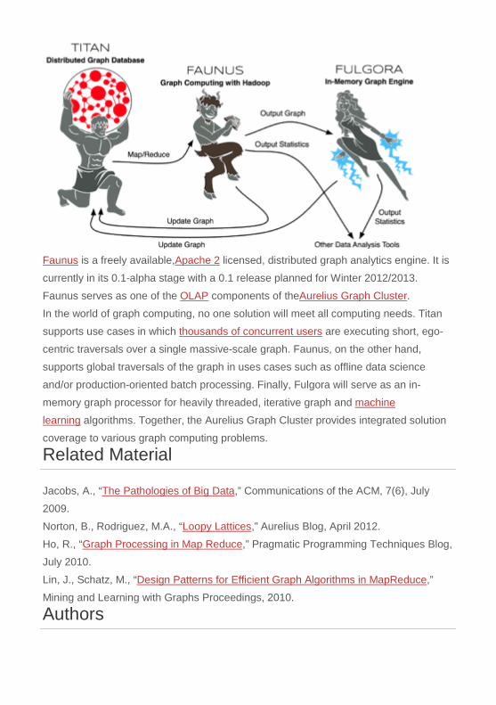
Faunus is a freely available,Apache 2 licensed, distributed graph analytics engine. It is

currently in its 0.1-alpha stage with a 0.1 release planned for Winter 2012/2013.

Faunus serves as one of the OLAP components of theAurelius Graph Cluster.

In the world of graph computing, no one solution will meet all computing needs. Titan

supports use cases in which thousands of concurrent users are executing short, ego-

centric traversals over a single massive-scale graph. Faunus, on the other hand,

supports global traversals of the graph in uses cases such as offline data science

and/or production-oriented batch processing. Finally, Fulgora will serve as an in-

memory graph processor for heavily threaded, iterative graph and machine

learning algorithms. Together, the Aurelius Graph Cluster provides integrated solution

coverage to various graph computing problems.

Related Material

Jacobs, A., “The Pathologies of Big Data,” Communications of the ACM, 7(6), July

2009.

Norton, B., Rodriguez, M.A., “Loopy Lattices,” Aurelius Blog, April 2012.

Ho, R., “Graph Processing in Map Reduce,” Pragmatic Programming Techniques Blog,

July 2010.

Lin, J., Schatz, M., “Design Patterns for Efficient Graph Algorithms in MapReduce,”

Mining and Learning with Graphs Proceedings, 2010.

Authors

FILED UNDER BLOG

A Solution to the Supernode Problem

OCTOBER 25, 2012 3 COMMENTS

In graph theory and network science, a

“supernode” is a vertex with a disproportionately high number of incident edges. While

supernodes are rare in natural graphs (as statistically demonstrated with power-

lawdegree distributions), they show up frequently during graph analysis. The reason

being is that supernodes are connected to so many other vertices that they exist on

numerous paths in the graph. Therefore, an arbitrary traversal is likely to touch a

supernode. In graph computing, supernodes can lead to system performance

problems. Fortunately, forproperty graphs, there is a theoretical and applied solution to

this problem.

Supernodes in the Real-World

Peer-to-Peer File Sharing

At the turn of the millenium, online file sharing was being supported by

services like Napster andGnutella. Unlike Napster, Gnutella is a true peer-to-peer

system in that it has no central file index. Instead, a client’s search is sent to its

adjacent clients. If those clients don’t have the file, then the request propagates to their

adjacent clients, so forth and so on. As in any natural graph, a supernode is only a few

steps away. Therefore, in many peer-to-peer networks, supernode clients are quickly

inundated with search requests and in turn, a DoS is effected. Social Network Celebrities

President Barack Obama currently has 21,322,866 followers on Twitter.

When Obama tweets, that tweet must register in the activity streams of 21+ million

accounts. The Barack Obama vertex is considered a supernode. As an opposing

example, when Stephen Mallette tweets, only 59 streams need to be updated. Twitter

realizes this discrepancy and maintains different mechanisms for handling “the

Obamas” (i.e. the celebrities) and “the Stephens” (i.e. the plebeians) of the Twitter-

sphere.

Blueprints and Vertex Queries

Blueprints is a Java interface for graph-based software.

Various graph databases, in-memory graph engines, and batch-analytics

frameworks make use of Blueprints. In June 2012, Blueprints 2.x was released with

support for “vertex queries.” A vertex query is best explained with an example.

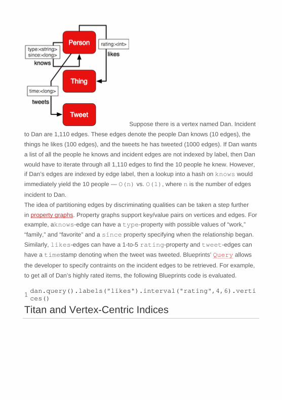
Suppose there is a vertex named Dan. Incident

to Dan are 1,110 edges. These edges denote the people Dan knows (10 edges), the

things he likes (100 edges), and the tweets he has tweeted (1000 edges). If Dan wants

a list of all the people he knows and incident edges are not indexed by label, then Dan

would have to iterate through all 1,110 edges to find the 10 people he knew. However, if Dan’s edges are indexed by edge label, then a lookup into a hash on knows would

immediately yield the 10 people — O(n) vs. O(1), where n is the number of edges

incident to Dan.

The idea of partitioning edges by discriminating qualities can be taken a step further

in property graphs. Property graphs support key/value pairs on vertices and edges. For example, aknows-edge can have a type-property with possible values of “work,”

“family,” and “favorite” and a since property specifying when the relationship began.

Similarly, likes-edges can have a 1-to-5 rating-property and tweet-edges can

have a timestamp denoting when the tweet was tweeted. Blueprints’ Query allows

the developer to specify contraints on the incident edges to be retrieved. For example,

to get all of Dan’s highly rated items, the following Blueprints code is evaluated.

1 dan.query().labels("likes").interval("rating",4,6).vertices() Titan and Vertex-Centric Indices

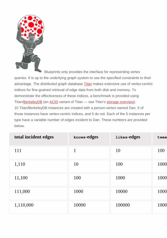
Blueprints only provides the interface for representing vertex

queries. It is up to the underlying graph system to use the specified constraints to their

advantage. The distributed graph database Titan makes extensive use of vertex-centric

indices for fine-grained retrieval of edge data from both disk and memory. To

demonstrate the effectiveness of these indices, a benchmark is provided using

Titan/BerkeleyDB (an ACID variant of Titan — see Titan’s storage overview).

10 Titan/BerkeleyDB instances are created with a person-vertex named Dan. 5 of

those instances have vertex-centric indices, and 5 do not. Each of the 5 instances per

type have a variable number of edges incident to Dan. These numbers are provided

below.

total incident edges knows-edges likes-edges tweet

111 1 10 100

1,110 10 100 1000

11,100 100 1000 10000

111,000 1000 10000 10000

1,110,000 10000 100000 10000

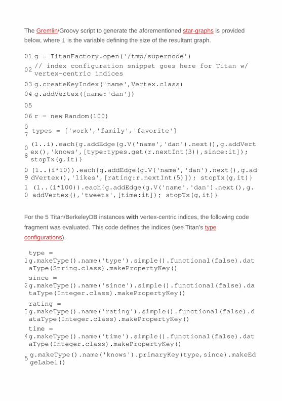
The Gremlin/Groovy script to generate the aforementioned star-graphs is provided below, where i is the variable defining the size of the resultant graph.

01 g = TitanFactory.open('/tmp/supernode')

02 // index configuration snippet goes here for Titan w/ vertex-centric indices 03 g.createKeyIndex('name',Vertex.class) 04 g.addVertex([name:'dan']) 05 06 r = new Random(100) 07 types = ['work','family','favorite']

08 (1..i).each{g.addEdge(g.V('name','dan').next(),g.addVertex(),'knows',[type:types.get(r.nextInt(3)),since:it]); stopTx(g,it)}

09 (1..(i*10)).each{g.addEdge(g.V('name','dan').next(),g.addVertex(),'likes',[rating:r.nextInt(5)]); stopTx(g,it)}

10

(1..(i*100)).each{g.addEdge(g.V('name','dan').next(),g.addVertex(),'tweets',[time:it]); stopTx(g,it)}

For the 5 Titan/BerkeleyDB instances with vertex-centric indices, the following code

fragment was evaluated. This code defines the indices (see Titan’s type

configurations).

1 type = g.makeType().name('type').simple().functional(false).dataType(String.class).makePropertyKey()

2 since = g.makeType().name('since').simple().functional(false).dataType(Integer.class).makePropertyKey()

3 rating = g.makeType().name('rating').simple().functional(false).dataType(Integer.class).makePropertyKey()

4 time = g.makeType().name('time').simple().functional(false).dataType(Integer.class).makePropertyKey()

5 g.makeType().name('knows').primaryKey(type,since).makeEdgeLabel()

6 g.makeType().name('likes').primaryKey(rating).makeEdgeLabel()

7 g.makeType().name('tweets').primaryKey(time).makeEdgeLabel()

Next, three traversals rooted at Dan are presented. The first gets all the people Dan

knows of a particular randomly chosen type (e.g. family members). The second returns

all of the things that Dan has highly rated (i.e. 4 or 5 star ratings). The third retrieves

Dan’s 10 most recent tweets. Finally, note that Gremlin compiles each expression to an

appropriate vertex query (see Gremlin’s traversal optimizations).

1 g.V('name','dan').outE('knows').has('type',types.get(r.nextInt(3)).inV

2 g.V('name','dan').outE('likes').interval('rating',4,6).inV

3 g.V('name','dan').outE('tweets').has('time',T.gt,(i*100)-10).inV

The traversals above were each run 25 times with the database

restarted after each query in order to demonstrate response times with

cold JVM caches. Note that in-memory, warm-cache response times show a similar

pattern (albeit relatively faster). The averaged results are plotted below where the y-

axis is on a log scale. The green, red, and blue colors denote the first, second and third

queries, respectively. Moreover, there is a light and a dark version of each color. The light version is Titan/BerkeleyDB without vertex-centric indices and the dark version is

Titan/BerkeleyDB with vertex-centric indices.

Perhaps the most impressive result is the retrieval of Dan’s 10 most recent tweets

(blue). With vertex-centric indices (dark blue), as the number of Dan’s tweets grow to 1

million, the time it takes to get the top 10 stays constant at around 1.5 milliseconds.

Without indices, this query grows proportionate to the amount of data and ultimately requires 13 seconds to complete (light blue). That is a 4 orders of magnitude difference in response time for the same result set. This example demonstrates

how useful vertex-centric indices are for activity stream-type systems.

The plot on the right

displays the number of vertices returned by each query over each graph size. As

expected, the number of tweets stays constant at 10 while the number

of knows and likes vertices retrieved grows proportionate to the growing graphs.

While the examples on the same graph (with and without indices) return the same

data, getting to that data is faster with vertex-centric indices.

Finally, Titan also supports composite key indices. The graph construction code fragment previous assigns a primary key of both type and since toknows-edges.

Therefore, retrieving Dan’s 10 most recent coworkers is more efficient than, in-memory, getting all of Dan’s coworkers and then sorting on since. The interested

reader can explore the runtimes of such composite vertex-centric queries by

augmenting the provided code snippets.

Conclusion

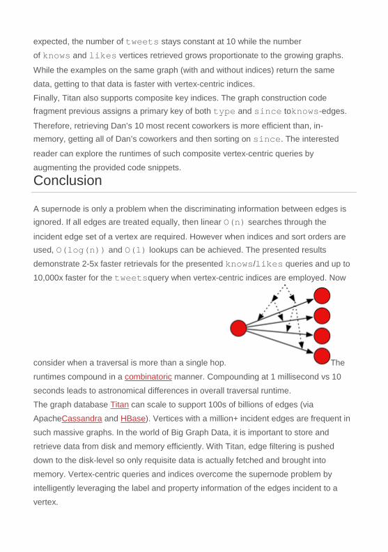
A supernode is only a problem when the discriminating information between edges is ignored. If all edges are treated equally, then linear O(n) searches through the

incident edge set of a vertex are required. However when indices and sort orders are used, O(log(n)) and O(1) lookups can be achieved. The presented results

demonstrate 2-5x faster retrievals for the presented knows/likes queries and up to

10,000x faster for the tweetsquery when vertex-centric indices are employed. Now

consider when a traversal is more than a single hop. The

runtimes compound in a combinatoric manner. Compounding at 1 millisecond vs 10

seconds leads to astronomical differences in overall traversal runtime.

The graph database Titan can scale to support 100s of billions of edges (via

ApacheCassandra and HBase). Vertices with a million+ incident edges are frequent in

such massive graphs. In the world of Big Graph Data, it is important to store and

retrieve data from disk and memory efficiently. With Titan, edge filtering is pushed

down to the disk-level so only requisite data is actually fetched and brought into

memory. Vertex-centric queries and indices overcome the supernode problem by

intelligently leveraging the label and property information of the edges incident to a

vertex.

Related Material

Rodriguez, M.A., Broecheler, M., “Titan: The Rise of Big Graph Data,” Public Lecture at

Jive Software, Palo Alto, 2012.

Broecheler, M., LaRocque, D., Rodriguez, M.A., “Titan Provides Real-Time Big Graph

Data,” Aurelius Blog, August 2012.

Authors

FILED UNDER BLOG

Deploying the Aurelius Graph Cluster

OCTOBER 17, 2012 1 COMMENT

The Aurelius Graph Cluster is a cluster of interoperable graph technologies that can be

deployed on a multi-machine compute cluster. This post demonstrates how to set up

the cluster on Amazon EC2 (a popular cloud service provider) with the following graph

technologies:

Titan is an Apache2-licensed distributed graph database that leverages

existing persistence technologies such as Apache HBase and Cassandra. Titan

implements the Blueprints graph API and therefore supports the Gremlin graph

traversal/query language. [OLTP]

Faunus is an Apache2-licensed batch analytics, graph computing

framework based on ApacheHadoop. Faunus leverages the Blueprints graph API and

exposes Gremlin as its traversal/query language. [OLAP] Please note the date of this publication. There may exist newer versions of the

technologies discussed as well as other deployment techniques. Finally, all commands

point to an example cluster and any use of the commands should be respective of the

specific cluster being computed on.

Cluster Configuration

The examples in this post assume the reader has

access to an Amazon EC2account. The first step is to create a machine instance that

has, at minimum,Java 1.6+ on it. This instance is used to spawn the graph cluster. The name given to this instance is agc-master and it is a modest m1.small machine.

On agc-master, Apache Whirr 0.8.0 is downloaded and unpacked.

1 ~$ ssh ubuntu@ec2-184-72-209-80.compute-1.amazonaws.com 2 ...

3 ubuntu@ip-10-117-55-34:~$ wget http://www.apache.org/dist/whirr/whirr-0.8.0/whirr-0.8.0.tar.gz

4 ubuntu@ip-10-117-55-34:~$ tar -xzf whirr-0.8.0.tar.gz

Whirr is a cloud service agnostic tool that simplifies the creation

and destruction of a compute cluster. A Whirr “recipe” (i.e. a properties file) describes

the machines in a cluster and their respective services. The recipe used in this post is

provided below and saved to a text file named agc.properties on agc-master.

The recipe defines a 5 m1.large machine cluster containing HBase 0.94.1 and Hadoop 1.0.3 (see whirr.instance-templates). HBase will serve as the

database persistance engine for Titan and Hadoop will serve as the batch computing

engine for Faunus.

01 whirr.cluster-name=agc

02 whirr.instance-templates=1 zookeeper+hadoop-namenode+hadoop-jobtracker+hbase-master,4 hadoop-datanode+hadoop-tasktracker+hbase-regionserver

03 whirr.provider=aws-ec2 04 whirr.identity=${env:AWS_ACCESS_KEY_ID} 05 whirr.credential=${env:AWS_SECRET_ACCESS_KEY} 06 whirr.hardware-id=m1.large 07 whirr.image-id=us-east-1/ami-da0cf8b3 08 whirr.location-id=us-east-1 09

whirr.hbase.tarball.url=http://archive.apache.org/dist/hbase/hbase-0.94.1/hbase-0.94.1.tar.gz

10

whirr.hadoop.tarball.url=http://archive.apache.org/dist/hadoop/core/hadoop-1.0.3/hadoop-1.0.3.tar.gz

11 hbase-site.dfs.replication=2 From agc-master, the following commands will launch the previously described

cluster. Note that the first two lines require specific Amazon EC2 account information.

When the launch completes, the Amazon EC2 web admin console will show the 5

m1.large machines.

1 ubuntu@ip-10-117-55-34:~$ export AWS_ACCESS_KEY_ID= # requires account specific information

2 ubuntu@ip-10-117-55-34:~$ export AWS_SECRET_ACCESS_KEY= # requires account specific information

3 ubuntu@ip-10-117-55-34:~$ ssh-keygen -t rsa -P ''

4 ubuntu@ip-10-117-55-34:~$ whirr-0.8.0/bin/whirr launch-cluster --config agc.properties

The

deployed cluster is diagrammed on the right where each machine maintains its

respective software services. The sections to follow will demonstrate how to load and

then process graph data within the cluster. Titan will serve as the data source for

Faunus’ batch analytic jobs.

Loading Graph Data into Titan

Titan is a highly scalable, distributed graph database that leverages

existing persistence engines. Titan 0.1.0 supports Apache Cassandra (AP),

Apache HBase (CP), and OracleBerkeleyDB (CA). Each of these backends

emphasizes a different aspect of the CAP theorem. For the purpose of this post,

Apache HBase is utilized and therefore, Titan is consistent (C) and partitioned (P). For the sake of simplicity, the 1 zookeeper+hadoop-namenode+hadoop-

jobtracker+hbase-master machine will be used for cluster interactions. The IP

address can be found in the Whirr instance metadata on agc-master. The reason

for using this machine is that numerous services are already installed on it (e.g.

HBase shell, Hadoop, etc.) and therefore, no manual software installation is required on agc-master.

1 ubuntu@ip-10-117-55-34:~$ more .whirr/agc/instances

2 us-east-1/i-3c121b41 zookeeper,hadoop-namenode,hadoop-jobtracker,hbase-master 54.242.14.83 10.12.27.208

3 us-east-1/i-34121b49 hadoop-datanode,hadoop-tasktracker,hbase-regionserver 184.73.57.182 10.40.23.46

4 us-east-1/i-38121b45 hadoop-datanode,hadoop-tasktracker,hbase-regionserver 54.242.151.125 10.12.119.135

5 us-east-1/i-3a121b47 hadoop-datanode,hadoop-tasktracker,hbase-regionserver 184.73.145.69 10.35.63.206

6 us-east-1/i-3e121b43 hadoop-datanode,hadoop-tasktracker,hbase-regionserver 50.16.174.157 10.224.3.16

Once in the machine via ssh, Titan 0.1.0 is downloaded, unzipped, and

the Gremlin console is started.

01 ubuntu@ip-10-117-55-34:~$ ssh 54.242.14.83 02 ...

03 ubuntu@ip-10-12-27-208:~$ wget https://github.com/downloads/thinkaurelius/titan/titan-0.1.0.zip

04 ubuntu@ip-10-12-27-208:~$ sudo apt-get install unzip 05 ubuntu@ip-10-12-27-208:~$ unzip titan-0.1.0.zip 06 ubuntu@ip-10-12-27-208:~$ cd titan-0.1.0/ 07 ubuntu@ip-10-12-27-208:~/titan-0.1.0$ bin/gremlin.sh 08 09 \,,,/ 10 (o o) 11 -----oOOo-(_)-oOOo----- 12 gremlin>

A toy 1 million vertex/edge graph is loaded into Titan using the Gremlin/Groovy script

below (simply cut-and-paste the source into the Gremlin console and wait

approximately 3 minutes). The code implements a preferential attachment algorithm.

For an explanation of this algorithm, please see the second column of page 33 in Mark Newman‘s article The Structure and Function of Complex Networks.

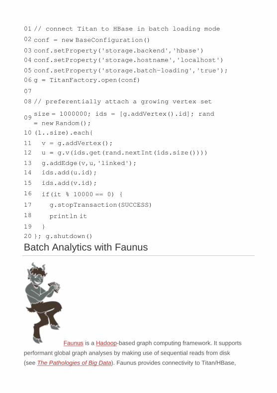
01 // connect Titan to HBase in batch loading mode 02 conf = new BaseConfiguration() 03 conf.setProperty('storage.backend','hbase') 04 conf.setProperty('storage.hostname','localhost') 05 conf.setProperty('storage.batch-loading','true'); 06 g = TitanFactory.open(conf) 07 08 // preferentially attach a growing vertex set

09 size = 1000000; ids = [g.addVertex().id]; rand = new Random();

10 (1..size).each{ 11 v = g.addVertex(); 12 u = g.v(ids.get(rand.nextInt(ids.size()))) 13 g.addEdge(v,u,'linked'); 14 ids.add(u.id); 15 ids.add(v.id); 16 if(it % 10000 == 0) { 17 g.stopTransaction(SUCCESS) 18 println it 19 } 20 }; g.shutdown() Batch Analytics with Faunus

Faunus is a Hadoop-based graph computing framework. It supports

performant global graph analyses by making use of sequential reads from disk (see The Pathologies of Big Data). Faunus provides connectivity to Titan/HBase,

Titan/Cassandra, any Rexster-fronted graph database, and to text/binary files stored in HDFS. From the 1 zookeeper+hadoop-namenode+hadoop-

jobtracker+hbase-master machine, Faunus 0.1-alpha is downloaded and

unzipped. The provided titan-hbase.properties file should be updated

withhbase.zookeeper.quorum=10.12.27.208 instead of localhost. The

IP address 10.12.27.208 is provided by ~/.whirr/agc/instances on agc-

master. Finally, the Gremlin console is started.

01

ubuntu@ip-10-12-27-208:~$ wget https://github.com/downloads/thinkaurelius/faunus/faunus-0.1-alpha.zip

02 ubuntu@ip-10-12-27-208:~$ unzip faunus-0.1-alpha.zip

03 ubuntu@ip-10-12-27-208:~$ cd faunus-0.1-alpha/

04 ubuntu@ip-10-12-27-208:~/faunus-0.1-alpha$ vi bin/titan-hbase.properties

05 ubuntu@ip-10-12-27-208:~/faunus-0.1-alpha$ bin/gremlin.sh

06 07 \,,,/ 08 (o o) 09 -----oOOo-(_)-oOOo----- 10 gremlin>

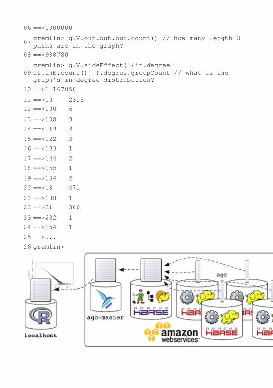
A few example Faunus jobs are provided below. The final job on line 9 generates an in-

degree distribution. The in-degree of a vertex is defined as the number of incoming

edges to the vertex. The outputted result states how many vertices (second column)

have a particular in-degree (first column). For example, 167,050 vertices have only 1

incoming edge.

01 gremlin> g = FaunusFactory.open('bin/titan-hbase.properties') 02 ==>faunusgraph[titanhbaseinputformat] 03 gremlin> g.V.count() // how many vertices in the graph? 04 ==>1000001 05 gremlin> g.E.count() // how many edges in the graph?

06 ==>1000000

07 gremlin> g.V.out.out.out.count() // how many length 3 paths are in the graph? 08 ==>988780

09 gremlin> g.V.sideEffect('{it.degree = it.inE.count()}').degree.groupCount // what is the graph's in-degree distribution?

10 ==>1 167050 11 ==>10 2305 12 ==>100 6 13 ==>108 3 14 ==>119 3 15 ==>122 3 16 ==>133 1 17 ==>144 2 18 ==>155 1 19 ==>166 2 20 ==>18 471 21 ==>188 1 22 ==>21 306 23 ==>232 1 24 ==>254 1 25 ==>... 26 gremlin>

To conclude, the in-degree distribution result is pulled from Hadoop’s HDFS (stored in output/job-0). Next, scp is used to download the file to agc-master and

then again to download the file to a local machine (e.g. a laptop). If the local machine

has R installed, then the file can be plotted and visualized (see the final diagram

below). The log-logplot demonstrates the known result that the preferential attachment

algorithm generates a graph with a power-lawdegree distribution (i.e. “natural

statistics”).

01 ubuntu@ip-10-12-27-208:~$ hadoop fs -getmerge output/job-0 distribution.txt 02 ubuntu@ip-10-12-27-208:~$ head -n5 distribution.txt 03 1 167050 04 10 2305 05 100 6 06 108 3 07 119 3 08 ubuntu@ip-10-12-27-208:~$ exit 09 ...

10 ubuntu@ip-10-117-55-34:~$ scp 54.242.14.83:~/distribution.txt . 11 ubuntu@ip-10-117-55-34:~$ exit 12 ...

13 ~$ scp ubuntu@ec2-184-72-209-80.compute-1.amazonaws.com:~/distribution.txt . 14 ~$ r 15 > t = read.table('distribution.txt') 16 > plot(t,log='xy',xlab='in-degree',ylab='frequency')

Conclusion

The Aurelius Graph Cluster is used for processing massive-scale graphs, where massive-scale denotes a graph so large it does not fit within the resource

confines of a single machine. In other words, the Aurelius Graph Cluster is all about

Big Graph Data. The two cluster technologies explored in this post

were Titan and Faunus. They serve two distinct graph computing needs. Titan supports

thousands of concurrent real-time, topologically local graph interactions. Faunus, on

the other hand, supports long running, topologically global graph analyses. In other

words, they provide OLTP and OLAP functionality, respectively.

References

London, G., “Set Up a Hadoop/HBase Cluster on EC2 in (About) an Hour,” Cloudera

Developer Center, October 2012.

Newman, M., “The Structure and Function of Complex Networks,” SIAM Review,

volume 45, pages 167-256, 2003.

Jacobs, A., “The Pathologies of Big Data,” ACM Communications, volume 7, number 6,

July 2009.

Authors

FILED UNDER BLOG

Titan Provides Real-Time Big Graph Data

AUGUST 6, 2012 6 COMMENTS

Titan is an Apache 2 licensed, distributed graph

database capable of supporting tens of thousands of concurrent users reading and

writing to a single massive-scalegraph. In order to substantiate the aforementioned

statement, this post presents empirical results of Titan backing a simulated social

networking site undergoing transactional loads estimated at 50,000–100,000

concurrent users. These users are interacting with 40 m1.small Amazon EC2 servers

which are transacting with a 6 machine Amazon EC2 cc1.4xl Titan/Cassandra cluster.

The presentation to follow discusses the simulation’s social graph structure, the types

of processes executed on that structure, and the various runtime analyses of those

processes under normal and peak load. The presentation concludes with a discussion

of the Amazon EC2 cluster architecture used and the associated costs of running that

architecture in a production environment. In short summary, Titan performs well under

substantial load with a relatively inexpensive cluster and as such, is capable of backing

online services requiring real-time Big Graph Data.

The Social Graph’s Structure and Processes

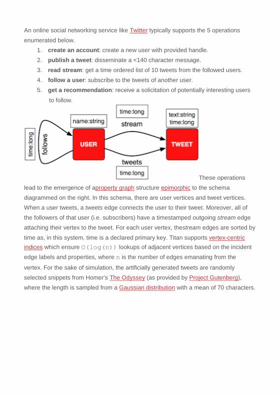
An online social networking service like Twitter typically supports the 5 operations

enumerated below. 1. create an account: create a new user with provided handle.

2. publish a tweet: disseminate a <140 character message.

3. read stream: get a time ordered list of 10 tweets from the followed users.

4. follow a user: subscribe to the tweets of another user.

5. get a recommendation: receive a solicitation of potentially interesting users

to follow.

These operations

lead to the emergence of aproperty graph structure epimorphic to the schema

diagrammed on the right. In this schema, there are user vertices and tweet vertices. When a user tweets, a tweets edge connects the user to their tweet. Moreover, all of

the followers of that user (i.e. subscribers) have a timestamped outgoing stream edge

attaching their vertex to the tweet. For each user vertex, thestream edges are sorted by

time as, in this system, time is a declared primary key. Titan supports vertex-centric indices which ensure O(log(n)) lookups of adjacent vertices based on the incident

edge labels and properties, where n is the number of edges emanating from the

vertex. For the sake of simulation, the artificially generated tweets are randomly

selected snippets from Homer’s The Odyssey (as provided by Project Gutenberg),

where the length is sampled from a Gaussian distribution with a mean of 70 characters.

To provide a foundational

layer of data, the Twitter graph as of 2009 was first loaded into the Titan cluster. This

data includes 41.7 million user vertices and 1.47 billion follows edges. After loading, the 40 m1.small machines are put into a “while(true)loop” (in fact, there are 10

concurrent threads on each worker running 125,000 iterations). During each iteration of

the loop, a worker selects an operation to enact using a biased coin toss (see the

diagram on the left). The distribution heavily favors stream reading as this is typically

the most prevalent operation in such online social systems. Next, if

arecommendation is provided, then there is a 30% chance that the user will follow one of the recommended users. This is how follows edges are added to the graph.

A follows recommendation (e.g. “who to follow“) makes use of the existing follows edges to determine, for a particular user, other users that they might

find interesting. Typically, some variant of a triangle closure is computed in such situations. In plain English, if the users that user A follows tend to follow user B, then it

is most likely that user B is a good user for user Ato follow. To capture this notion as a

real-time graph algorithm, the Gremlin graph traversal language is used.

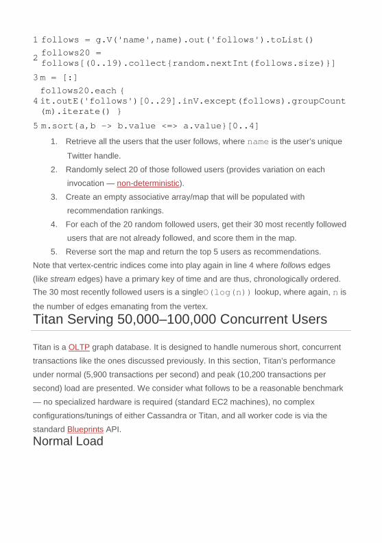
1 follows = g.V('name',name).out('follows').toList()

2 follows20 = follows[(0..19).collect{random.nextInt(follows.size)}]

3 m = [:]

4 follows20.each { it.outE('follows')[0..29].inV.except(follows).groupCount(m).iterate() }

5 m.sort{a,b -> b.value <=> a.value}[0..4] 1. Retrieve all the users that the user follows, where name is the user’s unique

Twitter handle.

2. Randomly select 20 of those followed users (provides variation on each

invocation — non-deterministic).

3. Create an empty associative array/map that will be populated with

recommendation rankings.

4. For each of the 20 random followed users, get their 30 most recently followed

users that are not already followed, and score them in the map.

5. Reverse sort the map and return the top 5 users as recommendations. Note that vertex-centric indices come into play again in line 4 where follows edges

(like stream edges) have a primary key of time and are thus, chronologically ordered. The 30 most recently followed users is a singleO(log(n)) lookup, where again, n is

the number of edges emanating from the vertex.

Titan Serving 50,000–100,000 Concurrent Users

Titan is a OLTP graph database. It is designed to handle numerous short, concurrent

transactions like the ones discussed previously. In this section, Titan’s performance

under normal (5,900 transactions per second) and peak (10,200 transactions per

second) load are presented. We consider what follows to be a reasonable benchmark

— no specialized hardware is required (standard EC2 machines), no complex

configurations/tunings of either Cassandra or Titan, and all worker code is via the

standard Blueprints API. Normal Load

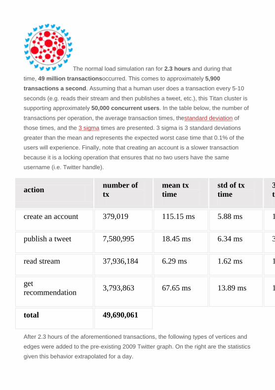
The normal load simulation ran for 2.3 hours and during that

time, 49 million transactionsoccurred. This comes to approximately 5,900 transactions a second. Assuming that a human user does a transaction every 5-10

seconds (e.g. reads their stream and then publishes a tweet, etc.), this Titan cluster is supporting approximately 50,000 concurrent users. In the table below, the number of

transactions per operation, the average transaction times, thestandard deviation of

those times, and the 3 sigma times are presented. 3 sigma is 3 standard deviations

greater than the mean and represents the expected worst case time that 0.1% of the

users will experience. Finally, note that creating an account is a slower transaction

because it is a locking operation that ensures that no two users have the same

username (i.e. Twitter handle).

action number of tx

mean tx time

std of tx time

3 ti

create an account 379,019 115.15 ms 5.88 ms 1

publish a tweet 7,580,995 18.45 ms 6.34 ms 3

read stream 37,936,184 6.29 ms 1.62 ms 1

get recommendation 3,793,863 67.65 ms 13.89 ms 1

total 49,690,061

After 2.3 hours of the aforementioned transactions, the following types of vertices and

edges were added to the pre-existing 2009 Twitter graph. On the right are the statistics

given this behavior extrapolated for a day.

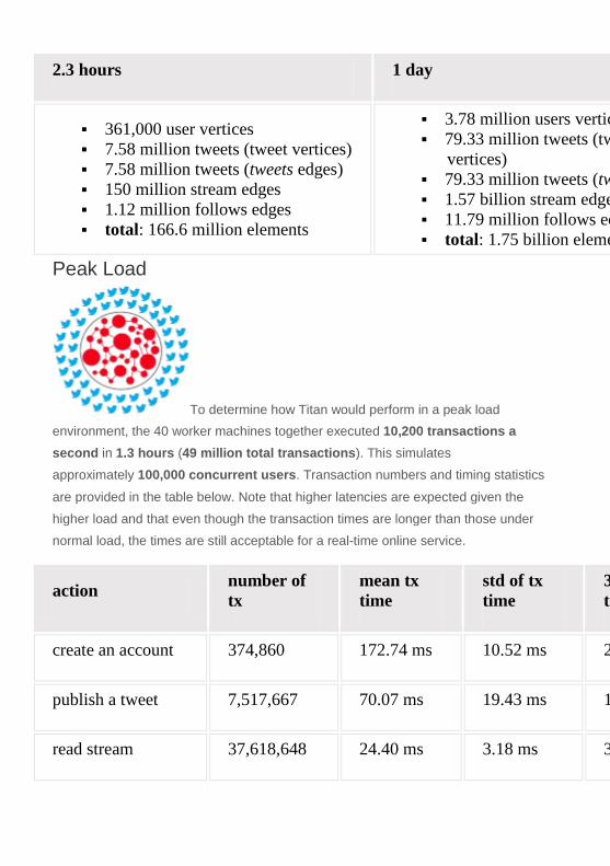
2.3 hours 1 day

361,000 user vertices 7.58 million tweets (tweet vertices) 7.58 million tweets (tweets edges) 150 million stream edges 1.12 million follows edges total: 166.6 million elements

3.78 million users vertic 79.33 million tweets (tw

vertices) 79.33 million tweets (tw 1.57 billion stream edge 11.79 million follows ed total: 1.75 billion eleme

Peak Load

To determine how Titan would perform in a peak load environment, the 40 worker machines together executed 10,200 transactions a second in 1.3 hours (49 million total transactions). This simulates

approximately 100,000 concurrent users. Transaction numbers and timing statistics

are provided in the table below. Note that higher latencies are expected given the

higher load and that even though the transaction times are longer than those under

normal load, the times are still acceptable for a real-time online service.

action number of tx

mean tx time

std of tx time

3 ti

create an account 374,860 172.74 ms 10.52 ms 2

publish a tweet 7,517,667 70.07 ms 19.43 ms 1

read stream 37,618,648 24.40 ms 3.18 ms 3

get recommendation 3,758,266 229.83 ms 29.08 ms 3

total 49,269,441

Amazon EC2 Machinery and Costs

The simulation presented was executed

on Amazon EC2. The software infrastructure to run this simulation made use

of CloudFormation. In terms of the hardware infrastructure, this section discusses

theinstance types, their physical statistics during the experiment, and the cost of

running this architecture in a production environment.

The 40 workers were m1.small Amazon EC2 instances (1.7 GB of memory with 1

virtual core). The Titan/Cassandra cluster was composed of 6 machines each with the

following specification.

23 GB of memory

33.5 EC2 Compute Units (2 x Intel Xeon X5570, quad-core “Nehalem”

architecture)

1,690 GB of storage

64-bit platform

10 Gigabit Ethernet

EC2 API name: cc1.4xlarge

Under the normal load simulation, the 6 machine Titan cluster experienced the

following CPU utilization, disk reads (in bytes), and disk writes (in bytes) — each

colored line represents 1 of the 6 cc1.4xlarge machines. Note that the disk read chart

is a 1 hour snapshot during the middle of the experiment and therefore, the caches are

warm. In summary, Titan is able to consistently, and without exertion, maintain the

normal transactional load.

The cost of running all these machines is provided in the table below. Note that in a

production environment (non-simulation), the 40 workers can be interpreted as web

servers taking user requests and processing results returned from the Titan cluster.

instance cost per hour cost per day cost pe

6 cc1.4xl $7.80 $187.20 $68,32

40 m1.small $3.20 $76.80 $28,03

total $11.00 $264.00 $96,36

For serving 50,000–100,000 concurrent users, $96,360 a year is inexpensive

considering incoming revenue seen from a user base of that size (assume 5% of the

user base is concurrent: ~2 million registered users). Moreover, Titan can be deployed

over an arbitrary number of machines and dynamically scale to meet load requirements

(seeThe Benefits of Titan). Therefore, this 6 cc1.4xl architecture is not a necessity, but

a particular configuration that was explored for the purpose of the presented social

simulation. For environments with less load, a smaller cluster can and should be used.

Conclusion

Titan has been in research and development for the past 4 years. In Spring 2012, Titan

was made freely available by Aurelius under the liberal Apache 2 license. It is currently

distributed as a 0.1-alpha with a 0.1 release planned by the end of Summer 2012.

Note that Titan is but one piece of the larger graph puzzle.

Titan serves the OLTPaspect of graph processing. By the middle of Fall 2012, Aurelius

will release a collection of OLAP graph technologies to support global graph

processing and analytics. All of the Aurelius technologies will integrate with one

another as well as with the suite of open source, BSD licensed graph technologies

provided byTinkerPop. By standing on the shoulders of giants (e.g. Cassandra,

TinkerPop, Amazon EC2), great leaps and bounds in applied graph theory and network

scienceare possible.

References

Kwak, H., Lee, C., Park, H., Moon, S., “What is Twitter, a Social Network or a News

Media?,” World Wide Web Conference, 2010.

Rodriguez, M.A., Broecheler, M., “Titan: The Rise of Big Graph Data,” Public Lecture at

Jive Software, Palo Alto, 2012.

Broecheler, M., LaRocque, D., Rodriguez, M.A., “Titan: A Highly Scalable, Distributed

Graph Database,” GraphLab Workshop 2012, San Francisco, 2012.

Authors

FILED UNDER BLOG

Structural Abstractions in Brains and Graphs

MAY 8, 2012 6 COMMENTS

A graph database is a software system that persists and represents data as a

collection of vertices (i.e. nodes, dots) connected to one another by a collection of

edges (i.e. links, lines). These databases are optimized for executing a type of process

known as a graph traversal. At various levels of abstraction, both the structure and

function of a graph yield a striking similarity to neural systems such as the human

brain. It is posited that as graph systems scale to encompass more heterogenous data,

a multi-level structural understanding can help facilitate the study of graphs and the

engineering of graph systems. Finally, neuroscience may foster a realization and

appreciation of the various structural abstractions that exist within the graph.

The Neuron and the Vertex

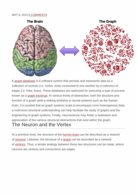
At a primitive level, the structure of the human brain can be described as a network

of neurons. Likewise, the structure of a graph can be described as a network

of vertices. Thus, a simple analogy between these two structures can be made, where

neurons are vertices and connections are edges.

The human brain is believed to be composed of approximately 100 billion neurons and

1 quadrillion connections (1 quadrillion is 1000 trillion). If the human brain was only

understood at the level of neurons, then the brain would be too complex to reason

about. Similarly, if a graph of 100 billion interconnected vertices was only studied from

the vantage point of vertices and edges, then the structure would be too overwhelming

to grasp. To combat this problem, in both cognitive neuroscience and network science,

it is typical to abstract away the low-level connectivity patterns in order to realize larger

functional structures. In neuroscience, some techniques used to do this are itemized

below. Neurons: Invasive microelectrodes can be used to measure the activity of a

single neuron (or small group of neurons) during the presentation of a

stimulus. Areas: Staining allows researchers to identify the metabolic

enzyme cytochrome oxidase and thus expose larger circuits participating in

the processing of sensory input. Regions: Non-invasive fMRI techniques leverage the magnetic aspects

of hemoglobin which is utilized by areas of the brain during a cognitive task or

presentation of stimuli.

In network science, algorithms exist to identify larger structures within the graph. Most

of the descriptive statistical algorithms developed are used for this purpose. Some of

these techniques are itemized below. Vertices: Measuring degree or centrality scores help to identify a vertex’s role

within the larger graph. Motifs: It is possible to identify lines, trees, cycles, cliques, etc. which are

associated with known functions.

Subgraphs: Leveraging community detection algorithms or graph minors help

to locate large structural areas within the graph that have high intra-

connectivity and low inter-connectivity.

In general, in order to have a well-rounded understanding of either the brain or the

graph, abstractions over its structure are required.

The Area and the Motif

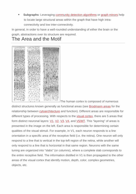
The human cortex is composed of numerous

distinct structures known generally as functional areas (see Brodmann areas for the

relationship between cytoarchitecture and function). Different areas are responsible for

different types of processing. With respects to the visual cortex, there are 5 areas that

form distinct neuronal layers: V1, V2, V3, V4, and V5/MT. This “layering” of areas is

presented in the image on the left. Each area is responsible for determining certain

qualities of the visual stimuli. For example, in V1, each neuron responds to a line

orientation in a specific area of the receptive field (i.e. the retina). One neuron will only

respond to a line that is vertical in the top-left region of the retina, while another will

only respond to a line that is horizontal in that same region. Neurons with the same

tuning are organized into “slabs” (or columns), where a complete slab corresponds to

the entire receptive field. The information distilled in V1 is then propagated to the other

areas of the visual cortex that identify motion, depth, color, complex geometries,

objects, etc.

In analogy to the brain’s functional areas, functional motifs can be identified in real-

world graphs. Motifs are prevalent in a type of graph known as a multi-relational graph.

A multi-relational graph is composed of a set of heterogenous vertices (e.g. people,

webpages, categories) and a set of directed labeled edges (e.g. friend, wrote, read,

broader). The Wikipedia graph, made freely available by DBPedia, is an excellent

example of a multi-relational graph containing numerous motifs. In particular,

a taxonomical motif is found in its category system (note that the Wikipedia category

system is not a directed acyclic graph). In this taxonomy, there are high-level categories such ascognition (the red vertices). Cognition is refined by more

specific categories: intelligence, reasoning,perception, etc. Ultimately, at

the lowest-level, Wikipedia pages (the purple vertices) have subject-edges

projecting to the vertices in the taxonomy that best represent them (typically to

categories lower in the taxonomy). Similar to how sensory input stimulates the

functional areas of the visual cortex, Wikipedia’s taxonomy can be stimulated by user usage. For example, a Wikipedia user (the green vertex) may click on the human

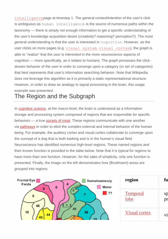
intelligencepage at timestep 1. The general context/intention of the user’s click

is ambiguous as human intelligence is the source of numerous paths within the

taxonomy — there is simply not enough information to get a specific understanding of

the user’s knowledge acquisition desire (creativity? reasoning? perception?). The most general understanding is that the user is interested in cognition. However, as the

user clicks on more pages (e.g. visual system, visual cortex), the graph is

able to “realize” that the user is interested in the more neuroscience aspects of

cognition — more specifically, as it relates to humans. The graph processes the click-

stream behavior of the user in order to converge upon a category (or set of categories)

that best represents that user’s information searching behavior. Note that Wikipedia

does not leverage this algorithm as it is primarily a static representational structure.

However, in order to draw an analogy to signal processing in the brain, this usage

example was presented.

The Region and the Subgraph

In cognitive science, at the macro-level, the brain is understood as a information

storage and processing system composed of regions that are responsible for specific

behaviors — a true society of mind. These regions communicate with one another

via pathways in order to elicit the complex external and internal behavior of the human

being. For example, the auditory cortex and visual cortex collaborate to converge upon

the concept of a dog that is both barking and is in the human’s visual field.

Neuroscience has identified numerous high-level regions. These named regions and

their known function is provided in the table below. Note that it is typical for regions to

have more than one function. However, for the sake of simplicity, only one function is

presented. Finally, the image on the left demonstrates how (Brodmann) areas are

grouped into regions.

region fu

Temporal lobe

sp pro

Visual cortex vis

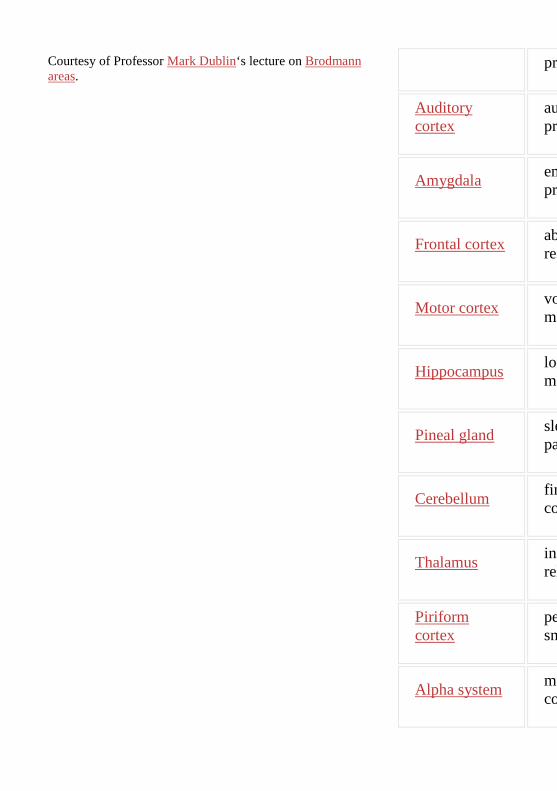
Courtesy of Professor Mark Dublin‘s lecture on Brodmann areas.

pro

Auditory cortex

au pro

Amygdala

em pro

Frontal cortex

ab rea

Motor cortex

vo mo

Hippocampus

lon me

Pineal gland

sle pa

Cerebellum

fin co

Thalamus

inf rel

Piriform cortex

pe sm

Alpha system

mu co

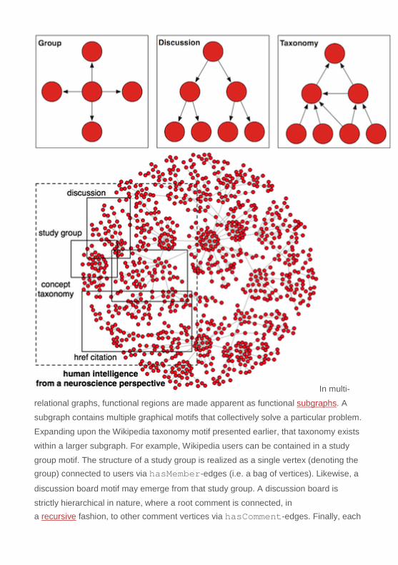
In multi-

relational graphs, functional regions are made apparent as functional subgraphs. A

subgraph contains multiple graphical motifs that collectively solve a particular problem.

Expanding upon the Wikipedia taxonomy motif presented earlier, that taxonomy exists

within a larger subgraph. For example, Wikipedia users can be contained in a study

group motif. The structure of a study group is realized as a single vertex (denoting the group) connected to users via hasMember-edges (i.e. a bag of vertices). Likewise, a

discussion board motif may emerge from that study group. A discussion board is

strictly hierarchical in nature, where a root comment is connected, in a recursive fashion, to other comment vertices via hasComment-edges. Finally, each

of those comments may have projections/links to Wikipedia pages or categories that

expand on the ideas presented in the comment. The aggregation of these motifs form a

functional subgraph whose purpose is to understand human intelligence from a

neuroscience perspective.

Conclusion

This post presented three structural abstractions found in human brains and in multi-

relational graphs. The purpose of structural abstraction is to aid researchers and

engineers in the understanding and design of complex systems. The graph database

space is developing infrastructure capable of representing and processing a variegated

information landscape within a single, unified, atomic graph structure. As this proceeds,

it will become more important to think in terms of structural abstractions in order to

better reason about the graph and to develop algorithms that are better able to

leverage it for collective problem-solving. In many ways, this is analogous to how the

human brain’s structures and processes are leveraged for individual problem-solving.

Acknowledgement

The images that are not directly referenced were provided by Wikipedia or generated

by the author.

References

Radomski, M., “Human Brain Capacity in Terabytes,” Mark Radomski’s WordPress

Blog, May 2008.

Best, B., “Basic Cerebral Cortex Function with Emphasis on Vision,” The Anatomical

Basis of Mind, 2004.

Rodriguez, M.A., “Graphs, Brains, and Gremlin,” Marko A. Rodriguez’s WordPress

Blog, July 2011.

Bollen, J., Van de Sompel, H., Hagberg, A., Bettencourt, L.M.A, Chute, R., Rodriguez,

M.A., Balakireva, L.L., “Clickstream Data Yields High-Resolution Maps of Science,”

PLoS One, Public Library of Science, 4(3), e4803, 2009.

Rodriguez, M.A., Ham, M.I., Gintautas, V., Kunsberg, B.S., “A Prospectus on the

Obstacles Inhibiting the Implementation of Advanced Artificial Neural Systems – Part

1,” Decade of Mind IV Conference, Albuquerque, New Mexico, January 2009.

Ham, M.I., Gintautas, V., Rodriguez, M.A., Bennett, R.A., Santa Maria, C.L.,

Bettencourt, L.M.A., “Density-Dependence of Functional Development in Spiking

Cortical Networks Grown in Vitro,” Biological Cybernetics, 102(1), pp. 71-80, March

2010.

Rodriguez, M.A., “From the Signal to the Symbol: Structure and Process in Artificial

Intelligence,” PostDoctoral Public Lecture at the Center for Nonlinear Studies, Los

Alamos National Laboratory, November 2008.

Minsky, M., “Society of Mind,” Simon & Schuster Press, March 1988.

Heylighen, F., “Collective Intelligence and its Implementation on the Web,” Journal of

Computational and Mathematical Organization Theory, 5(3), October 1999.

Author

FILED UNDER BLOG

Loopy Lattices

APRIL 21, 2012 2 COMMENTS

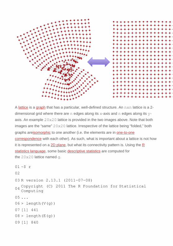
A lattice is a graph that has a particular, well-defined structure. An nxn lattice is a 2-

dimensional grid where there are n edges along its x-axis and n edges along its y-

axis. An example 20x20 lattice is provided in the two images above. Note that both

images are the “same” 20x20 lattice. Irrespective of the lattice being “folded,” both

graphs areisomorphic to one another (i.e. the elements are in one-to-one

correspondence with each other). As such, what is important about a lattice is not how

it is represented on a 2D plane, but what its connectivity pattern is. Using the R

statistics language, some basic descriptive statistics are computed for the 20x20 lattice named g.

01 ~$ r 02 03 R version 2.13.1 (2011-07-08)

04 Copyright (C) 2011 The R Foundation for Statistical Computing

05 ... 06 > length(V(g)) 07 [1] 441 08 > length(E(g)) 09 [1] 840

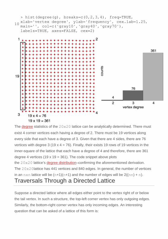
10 > hist(degree(g), breaks=c(0,2,3,4), freq=TRUE, xlab='vertex degree', ylab='frequency', cex.lab=1.25, main='', col=c('gray10','gray40','gray70'), labels=TRUE, axes=FALSE, cex=2)

The degree statistics of the 20x20 lattice can be analytically determined. There must

exist 4 corner vertices each having a degree of 2. There must be 19 vertices along

every side that each have a degree of 3. Given that there are 4 sides, there are 76

vertices with degree 3 (19 x 4 = 76). Finally, their exists 19 rows of 19 vertices in the

inner-square of the lattice that each have a degree of 4 and therefore, there are 361

degree 4 vertices (19 x 19 = 361). The code snippet above plots the 20x20 lattice’s degree distribution–confirming the aforementioned derivation.

The 20x20lattice has 441 vertices and 840 edges. In general, the number of vertices

in an nxn lattice will be (n+1)(n+1) and the number of edges will be 2((nn) + n).

Traversals Through a Directed Lattice

Suppose a directed lattice where all edges either point to the vertex right of or below

the tail vertex. In such a structure, the top-left corner vertex has only outgoing edges.

Similarly, the bottom-right corner vertex has only incoming edges. An interesting

question that can be asked of a lattice of this form is:

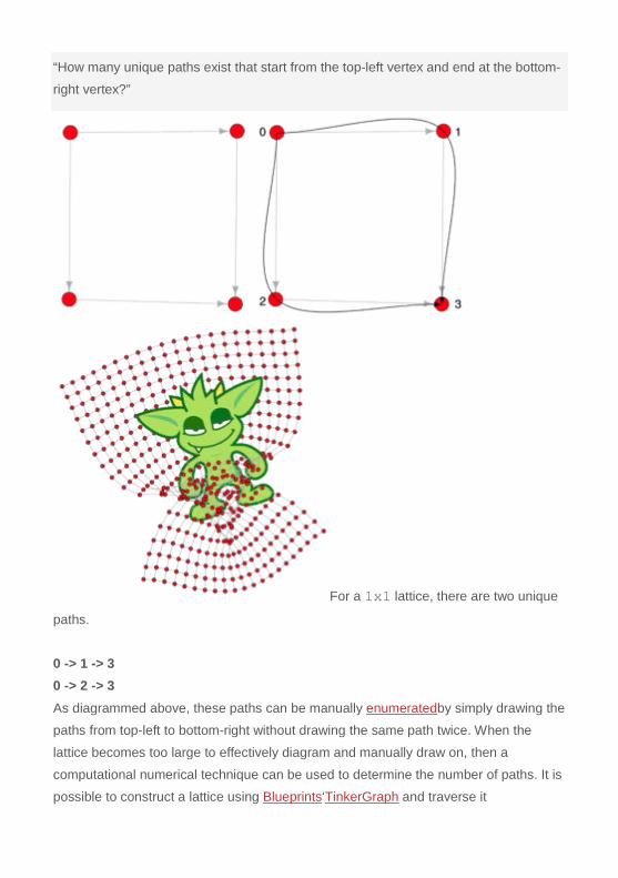
“How many unique paths exist that start from the top-left vertex and end at the bottom-

right vertex?”

For a 1x1 lattice, there are two unique

paths.

0 -> 1 -> 3

0 -> 2 -> 3

As diagrammed above, these paths can be manually enumeratedby simply drawing the

paths from top-left to bottom-right without drawing the same path twice. When the

lattice becomes too large to effectively diagram and manually draw on, then a

computational numerical technique can be used to determine the number of paths. It is

possible to construct a lattice using Blueprints‘TinkerGraph and traverse it

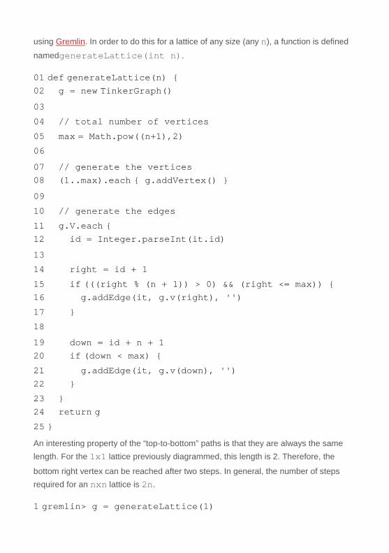
using Gremlin. In order to do this for a lattice of any size (any n), a function is defined

namedgenerateLattice(int n).

01 def generateLattice(n) { 02 g = new TinkerGraph() 03 04 // total number of vertices 05 max = Math.pow((n+1),2) 06 07 // generate the vertices 08 (1..max).each { g.addVertex() } 09 10 // generate the edges 11 g.V.each { 12 id = Integer.parseInt(it.id) 13 14 right = id + 1 15 if (((right % (n + 1)) > 0) && (right <= max)) { 16 g.addEdge(it, g.v(right), '') 17 } 18 19 down = id + n + 1 20 if (down < max) { 21 g.addEdge(it, g.v(down), '') 22 } 23 } 24 return g 25 } An interesting property of the “top-to-bottom” paths is that they are always the same length. For the 1x1 lattice previously diagrammed, this length is 2. Therefore, the

bottom right vertex can be reached after two steps. In general, the number of steps required for an nxn lattice is 2n.

1 gremlin> g = generateLattice(1)

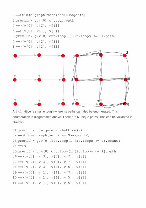
2 ==>tinkergraph[vertices:4 edges:4] 3 gremlin> g.v(0).out.out.path 4 ==>[v[0], v[2], v[3]] 5 ==>[v[0], v[1], v[3]] 6 gremlin> g.v(0).out.loop(1){it.loops <= 2}.path 7 ==>[v[0], v[2], v[3]] 8 ==>[v[0], v[1], v[3]]

A 2x2 lattice is small enough where its paths can also be enumerated. This

enumeration is diagrammed above. There are 6 unique paths. This can be validated in

Gremlin.

01 gremlin> g = generateLattice(2) 02 ==>tinkergraph[vertices:9 edges:12] 03 gremlin> g.v(0).out.loop(1){it.loops <= 4}.count() 04 ==>6 05 gremlin> g.v(0).out.loop(1){it.loops <= 4}.path 06 ==>[v[0], v[3], v[6], v[7], v[8]] 07 ==>[v[0], v[3], v[4], v[7], v[8]] 08 ==>[v[0], v[3], v[4], v[5], v[8]] 09 ==>[v[0], v[1], v[4], v[7], v[8]] 10 ==>[v[0], v[1], v[4], v[5], v[8]] 11 ==>[v[0], v[1], v[2], v[5], v[8]]

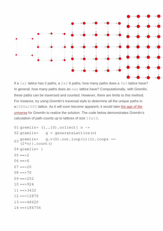
If a 1x1 lattice has 2 paths, a 2x2 6 paths, how many paths does a 3x3 lattice have?

In general, how many paths does an nxn lattice have? Computationally, with Gremlin,

these paths can be traversed and counted. However, there are limits to this method.

For instance, try using Gremlin’s traversal style to determine all the unique paths in a1000x1000 lattice. As it will soon become apparent, it would take the age of the

universe for Gremlin to realize the solution. The code below demonstrates Gremlin’s calculation of path counts up to lattices of size 10x10.

01 gremlin> (1..10).collect{ n -> 02 gremlin> g = generateLattice(n)

03 gremlin> g.v(0).out.loop(1){it.loops <= (2*n)}.count()

04 gremlin> } 05 ==>2 06 ==>6 07 ==>20 08 ==>70 09 ==>252 10 ==>924 11 ==>3432 12 ==>12870 13 ==>48620 14 ==>184756

A Closed Form Solution and the Power of Analytical Techniques

In order to know the number of paths through any arbitrary nxn lattice, a closed form

equation must be derived. One way to determine the closed form equation is to simply

search for the sequence on Google. The first site returned is the Online Encyclopedia

of Integer Sequences. The sequence discovered by Gremlin is called A000984 and

there exists the following note on the page: “The number of lattice paths from (0,0) to (n,n) using steps (1,0) and (0,1).

[Joerg Arndt, Jul 01 2011]“

The same page states that the general form is “2n choose n.” This can be expanded

out to its factorialrepresentation (e.g. 5! = 5 * 4 * 3 * 2 * 1) as diagrammed below.

Given this closed form solution, an explicit graph structure does not need to be traversed. Instead, a combinatoricequation can be evaluated for any n. A

directed 20x20 lattice has over 137 billion unique paths! This number of paths is

simply too many for Gremlin to enumerate in a reasonable amount of time.

1 > n = 20 2 > factorial(2 * n) / factorial(n)^2 3 [1] 137846528820

A question that can be asked is: “How does 2n choose 2 explain the number of paths through an nxn lattice?” When counting the number of paths from

vertex (0,0) to (n,n), where only down and right moves are allowed, there have to

be n moves down and n moves right. This means there are 2n total moves, and as

such, there are n choices (as the other n “choices” are forced by the

previous n choices). Thus, the total number of moves is “2n choose n.” This same

integer sequence is also found in another seemingly unrelated problem (provided by

the same web page).

“Number of possible values of a 2*n bit binary number for which half the bits are on and

half are off. – Gavin Scott, Aug 09 2003″

Each move is a sequence of letters that contains n Ds and n Rs, where down twice

then right twice would be DDRR. This maps the “lattice problem” onto the “binary string

of length 2n problem.” Both problems are essentially realizing the same behavior via

two different representations.

Plotting the Growth of a Function

It is possible to plot the combinatorial function over the sequence 1 to 20 (left plot below). What is interesting to note is that when the y-axis of the plot is set to a log-

scale, the plot is a straight line (right plot below). This means that the number of paths

in a directed lattice grows exponentially as the size of the lattice grows linear.

1 > factorial(2 * seq(1,n)) / factorial(seq(1,n))^2

2 [1] 2 6 20 70 252 924

3 [7] 3432 12870 48620 184756 705432 2704156

4 [13] 10400600 40116600 155117520 601080390 2333606220 9075135300 5 [19] 35345263800 137846528820 6 7 > x <- factorial(2 * seq(1,n)) / factorial(seq(1,n))^2

8 > plot(x, xlab='lattice size (n x n)', ylab='total number of paths', cex.lab=1.4, cex.axis=1.6, lwd=1.5, cex=1.5, type='b')

9 > plot(x, xlab='lattice size (n x n)', ylab="total

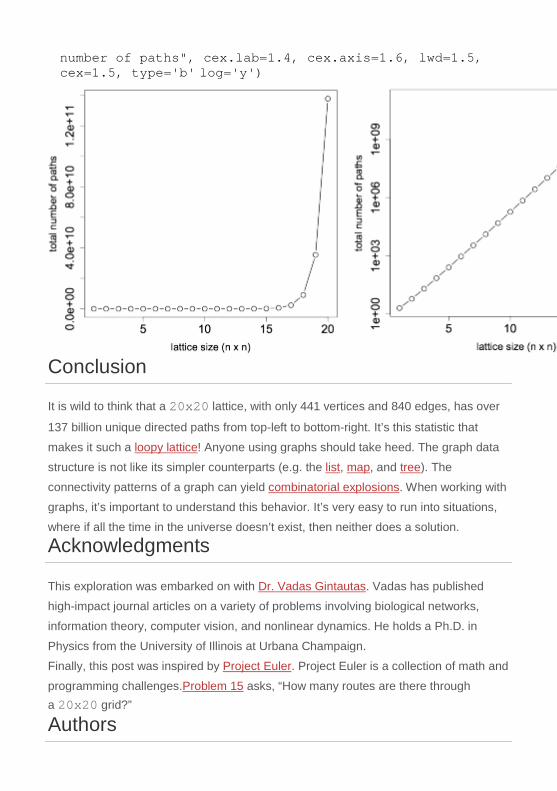
number of paths", cex.lab=1.4, cex.axis=1.6, lwd=1.5, cex=1.5, type='b' log='y')

Conclusion

It is wild to think that a 20x20 lattice, with only 441 vertices and 840 edges, has over

137 billion unique directed paths from top-left to bottom-right. It’s this statistic that

makes it such a loopy lattice! Anyone using graphs should take heed. The graph data

structure is not like its simpler counterparts (e.g. the list, map, and tree). The

connectivity patterns of a graph can yield combinatorial explosions. When working with

graphs, it’s important to understand this behavior. It’s very easy to run into situations,

where if all the time in the universe doesn’t exist, then neither does a solution.

Acknowledgments

This exploration was embarked on with Dr. Vadas Gintautas. Vadas has published

high-impact journal articles on a variety of problems involving biological networks,

information theory, computer vision, and nonlinear dynamics. He holds a Ph.D. in

Physics from the University of Illinois at Urbana Champaign.

Finally, this post was inspired by Project Euler. Project Euler is a collection of math and

programming challenges.Problem 15 asks, “How many routes are there through a 20x20 grid?”

Authors

FILED UNDER BLOG

Multitenant Graph Applications

APRIL 6, 2012 LEAVE A COMMENT

A multitenant software system is a system that supports any number of customers

within a single application instance. Typically, that single instance makes use of a

shared data set, where a customer’s data is properly separated from another’s. While

data separation is a crucial aspect of a multitenant application, there may be system-

wide (e.g. global) computations that require the consumption of all customer data (or

some subset thereof). If no such global operations are required, then a multitenant

application would instead be a multi-instance application, where each customer’s data

is contained in its own isolated silo. A few example multitenant applications are

itemized below.

A company’s confidential reports (e.g. market strategies or financial

information) in a Business Intelligence system is isolated from competitors

within the same application. However, public data (e.g. census, market, tax

data) is shared amongst and linked to by the various tenant data sets. As

such, the public data helps to enhance the usefulness of each company’s

respective private data.

A social network service guarantees user privacy while, in an access control

list (ACL) fashion, allows users to share their data with other trusted users

(e.g. friends) in the system.

Patient records in a multitenant electronic health record system can be

separated to ensure patient confidentiality. However, collective statistics can

be gleaned from the global data set in order to allow data analysts/scientists

to study population-wide health concerns.

Blueprints and PartitionGraph

TinkerPop’s Blueprints 1.2+ makes it easy to build

multitenant, graph-based applications. Blueprints is a graph database interface similar

to the JDBC of the relational databasecommunity. Blueprints is supported by various

graph databases including TinkerGraph, Neo4j,OrientDB, DEX, and InfiniteGraph. In

addition to providing a standard graph interface, Blueprints includes a collection of

graph wrappers. A graph wrapper takes an existing graph implementation, such as Neo4jGraph, and decorates it with new features. For example, wrapping a graph

implementation with ReadOnlyGraph prevents graph mutations.

The graph wrapper that enables multitenancy is called PartitionGraph. PartitionGraph separates the underlying graph into

different partitions/buckets. However, edges can link vertices in two separate partitions.

In this way, multitenancy is clearly realized, where a partition serves as the location for

a single tenant’s data. Moreover, data “cross-fertilization” is possible through

appropriately constrained inter-partition linking. The design ofPartitionGraph borrows heavily from the Named Graph data architecture

popularized by the Web of Data/Linked Data community. The remainder of this post will

demonstrate graph-based multitenancy by means of an Electronic Health Records (EHR) system example using PartitionGraph, the graph traversal/query

language Gremlin, and the colorful characters of TinkerPop.

Intra-Partition Electronic Health Records

The following code snippet demonstrates how PartitionGraph solves the multitenancy problem. First, a new graph is

constructed and wrapped in aPartitionGraph with an initial write partition

of pgp (Pipes General Practice). The graph used is the in-memory TinkerGraph. The

write partition is the partition that newly created data is written too. When patient

Gremlin goes to Pipes General Practice and TinkerPop Medical Center, two vertices are written to the pgp and tmc partitions, respectively.

01 ~$ gremlin 02 03 \,,,/ 04 (o o) 05 -----oOOo-(_)-oOOo-----

06 gremlin> g = new PartitionGraph(new TinkerGraph(), '_partition', 'pgp')

07 ==>partitiongraph[tinkergraph[vertices:0 edges:0]] 08 gremlin> g.getPartitionKey() 09 ==>_partition 10 gremlin> g.getReadPartitions() 11 ==>pgp

12 gremlin> g.getWritePartition() 13 ==>pgp

14 gremlin> gremlinPgp = g.addVertex('gremlin@pipesgeneralpractice') 15 ==>v[gremlin@pipesgeneralpractice] 16 gremlin> g.setWritePartition('tmc')

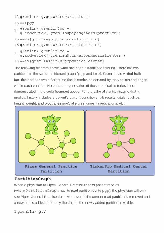
17 gremlin> gremlinTmc = g.addVertex('gremlin@tinkerpopmedicalcenter') 18 ==>v[gremlin@tinkerpopmedicalcenter] The following diagram shows what has been established thus far. There are two partitions in the same multitenant graph (pgp and tmc). Gremlin has visited both

facilities and has two different medical histories as denoted by the vertices and edges

within each partition. Note that the generation of those medical histories is not

demonstrated in the code fragment above. For the sake of clarity, imagine that a

medical history includes a patient’s current conditions, lab results, vitals (such as

height, weight, and blood pressure), allergies, current medications, etc.

When a physician at Pipes General Practice checks patient records (where PartitionGraph has its read partition set to pgp), the physician will only

see Pipes General Practice data. Moreover, if the current read partition is removed and

a new one is added, then only the data in the newly added partition is visible.

1 gremlin> g.V

2 ==>v[gremlin@pipesgeneralpractice] 3 gremlin> g.removeReadPartition('pgp') 4 gremlin> g.addReadPartition('tmc') 5 gremlin> g.V 6 ==>v[gremlin@tinkerpopmedicalcenter] At this point, the example has shown how to firewall customer data with PartitionGraph. Next, it is possible to go beyond simply separating graph

elements into partitions. Edges may either be intra- or inter- partition in that they can

point to vertices in the same partition or to vertices in two different partitions. In this

way, it is possible to introduce global data that can be shared amongst all customers.

Inter-Partition Electronic Health Records

The following code fragment introduces a new snomed partition,

where snomed refers to the publicly availableSNOMED-CT clinical terms data set.

Example terms include pneumonia, common cold, acute nasal catarrh, etc. Vertices and edges are added to the snomed partition that represent the SNOMED-CT concept

hierarchy. Note that in practice, the full SNOMED-CT data set would be parsed into the

partition, but for this simple example, two clinical terms and

their subsumption relationship are written.

1 gremlin> g.setWritePartition('snomed')

2 gremlin> painInRightLeg = g.addVertex('snomed:287048003', [name:'Pain in right leg (finding)'])

3 ==>v[snomed:287048003]

4 gremlin> painInLowerLimb = g.addVertex('snomed:10601006', [name:'Pain in lower limb (finding)'])

5 ==>v[snomed:10601006]

6 gremlin> g.addEdge(painInRightLeg, painInLowerLimb, 'broader') 7 ==>e[0][snomed:287048003-broader->snomed:10601006] When patient Gremlin complains of an injured leg at both Pipes General Practice and

TinkerPop Medical Center, edges are added that connect the patient vertex to the respective clinical term vertex in the snomed partition. ThesecomplainedOf edges

are denoted by the dashed lines in the diagram below.

1 gremlin> g.setWritePartition('pgp')

2 gremlin> g.addEdge(gremlinPgp, painInRightLeg, 'complainedOf')

3 ==>e[1][gremlin@pipesgeneralpractice-complainedOf->snomed:287048003] 4 gremlin> g.setWritePartition('tmc')

5 gremlin> g.addEdge(gremlinTmc, painInRightLeg, 'complainedOf')

6 ==>e[2][gremlin@tinkerpopmedicalcenter-complainedOf->snomed:287048003]

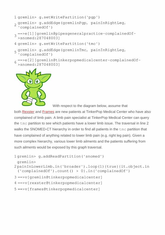
With respect to the diagram below, assume that

both Rexster and Frames are new patients at TinkerPop Medical Center who have also

complained of limb pain. A limb pain specialist at TinkerPop Medical Center can query the tmc partition to see which patients have a lower limb issue. The traversal in line 2

walks the SNOMED-CT hierarchy in order to find all patients in the tmc partition that

have complained of anything related to lower limb pain (e.g. right leg pain). Given a

more complex hierarchy, various lower limb ailments and the patients suffering from

such ailments would be exposed by this graph traversal.

1 gremlin> g.addReadPartition('snomed')

2 gremlin> painInLowerLimb.in('broader').loop(1){true}{it.object.in('complainedOf').count() > 0}.in('complainedOf')

3 ==>v[gremlin@tinkerpopmedicalcenter] 4 ==>v[rexster@tinkerpopmedicalcenter] 5 ==>v[frames@tinkerpopmedicalcenter]

Over a rich EHR data set, various other types of graph queries can be enacted. A few

examples are itemized below.

Determine what treatments were used on patients suffering from the same

lower limb ailment as Gremlin.

Correlate the personal medical histories of all lower limb patients to see if

there is a relationship amongst them (e.g. smoking, obesity, medical

prescriptions, etc.).

Find related clinical terms in SNOMED-CT and locate other patients that have

similar problems (e.g. numbness of the leg, sciatica, etc.). Determine what

treatments were successful for those related patients.

Connect patient Gremlin’s records at both Pipes General Practice and

TinkerPop Medical Center in order to create a unified perspective of Gremlin’s medical history via a sameAs edge (represented by the dash-

dotted line in the diagram above).

Conclusion

The benefit of PartitionGraph is that global data does not introduce significant

complexity to the programming model nor does it expose risks to firewalled partitions.

Moreover, it is possible to enact graph-wide analyses that span all partitions. This can

be a compelling advantage for Business Intelligence applications. Given the running

example, by simply making all partitions readable, it is possible to analyze the medical

histories across all medical facilities and leverage the SNOMED-CT data as the bridge

between these seemingly disparate partitioned data sets.

01 gremlin> g.addReadPartition('pgp') 02 gremlin> g.addReadPartition('tmc') 03 gremlin> g.addReadPartition('snomed') 04 gremlin> g.V 05 ==>v[rexster@tinkerpopmedicalcenter] 06 ==>v[snomed:287048003] 07 ==>v[frames@tinkerpopmedicalcenter] 08 ==>v[snomed:10601006] 09 ==>v[gremlin@tinkerpopmedicalcenter] 10 ==>v[gremlin@pipesgeneralpractice] 11 gremlin> g.E

12 ==>e[3][rexster@tinkerpopmedicalcenter-complainedOf->snomed:287048003]

13 ==>e[2][gremlin@tinkerpopmedicalcenter-complainedOf->snomed:287048003]

14 ==>e[1][gremlin@pipesgeneralpractice-complainedOf->snomed:287048003] 15 ==>e[0][snomed:287048003-broader->snomed:10601006]

16 ==>e[4][gremlin@tinkerpopmedicalcenter-sameAs->gremlin@pipesgeneralpractice]

17 ==>e[5][frames@tinkerpopmedicalcenter-complainedOf->snomed:287048003] PartitionGraph presents interesting opportunities for analyses that mix and

match different partitions in a traversal space. To conclude, a collection of more

complex EHR medical use cases are presented that can be conveniently facilitated by PartitionGraph.

A cross medical facility (i.e. partition) analysis shows that the percentage of

patients with HIV/AIDS who are prescribed an antiretroviral drug is below

standards set forth by the Centers for Medicare and Medicaid Services’

(CMS) quality measures. This analysis prompts healthcare providers and

administrators to consider changes to treatment protocols and drug

formularies.

Physician communities of practice can be identified by analyzing patient visit

and treatment patterns. Given those communities, it is possible

for pharmaceutical companies to predict the influencers within the greater

physician social network in order to yield insight into potential drug adoption

patterns.

Patient records across all partitions provides the foundational data set for a

population-wide analysis within a clinical decision support system.

Authors

FILED UNDER BLOG

Understanding the World using Tables and Graphs

MARCH 22, 2012 LEAVE A COMMENT

Organizations make use of data to drive their decision making, enhance their product

features, and to increase the efficiency of their everyday operations. Data by itself is

not useful. However, with data analysis, patterns such as trends, clusters, predictions,

etc. can be distilled. The way in which data is analyzed is predicated on the way in

which data is structured. The table format popularized by spreadsheets and relational

databases is useful for particular types of processing. However, the primary purpose of

this post is to examine a relatively less exploited structure that can be leveraged when

analyzing an organization’s data — the graph/network.

The Table Perspective

Before discussing graphs, a short review of the table data structure is presented using

a toy example containing a 12 person population. For each individual person, their

name, age, and total spending for the year is gathered. TheR Statistics code snippet

below loads the population data into a table.

> people <- read.table(file='people.txt', sep='\t',

header=TRUE)

> people

id name age spending

1 0 francis 57 100000

2 1 johan 37 150000

3 2 herbert 56 150000

4 3 mike 34 30000

5 4 richard 47 35000

6 5 alberto 31 70000

7 6 stephan 36 90000

8 7 dan 52 40000

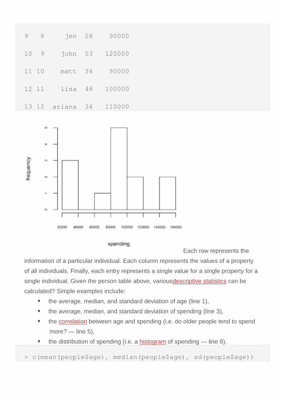
9 8 jen 28 90000

10 9 john 53 120000

11 10 matt 34 90000

12 11 lisa 48 100000

13 12 ariana 34 110000

Each row represents the

information of a particular individual. Each column represents the values of a property

of all individuals. Finally, each entry represents a single value for a single property for a

single individual. Given the person table above, variousdescriptive statistics can be

calculated? Simple examples include:

the average, median, and standard deviation of age (line 1),

the average, median, and standard deviation of spending (line 3),

the correlation between age and spending (i.e. do older people tend to spend

more? — line 5),

the distribution of spending (i.e. a histogram of spending — line 8).

> c(mean(people$age), median(people$age), sd(people$age))

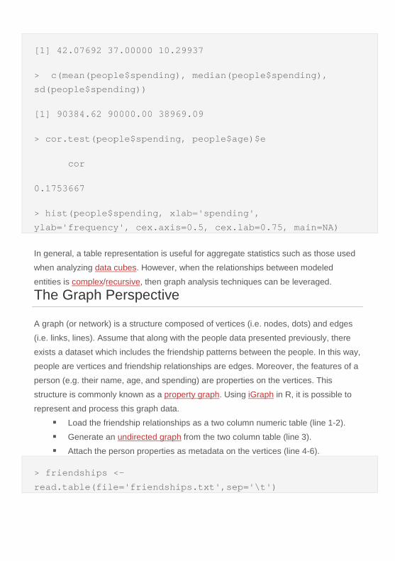
[1] 42.07692 37.00000 10.29937

> c(mean(people$spending), median(people$spending),

sd(people$spending))

[1] 90384.62 90000.00 38969.09

> cor.test(people$spending, people$age)$e

cor

0.1753667

> hist(people$spending, xlab='spending',

ylab='frequency', cex.axis=0.5, cex.lab=0.75, main=NA)

In general, a table representation is useful for aggregate statistics such as those used

when analyzing data cubes. However, when the relationships between modeled

entities is complex/recursive, then graph analysis techniques can be leveraged.

The Graph Perspective

A graph (or network) is a structure composed of vertices (i.e. nodes, dots) and edges

(i.e. links, lines). Assume that along with the people data presented previously, there

exists a dataset which includes the friendship patterns between the people. In this way,

people are vertices and friendship relationships are edges. Moreover, the features of a

person (e.g. their name, age, and spending) are properties on the vertices. This

structure is commonly known as a property graph. Using iGraph in R, it is possible to

represent and process this graph data.

Load the friendship relationships as a two column numeric table (line 1-2).

Generate an undirected graph from the two column table (line 3).

Attach the person properties as metadata on the vertices (line 4-6).

> friendships <-

read.table(file='friendships.txt',sep='\t')

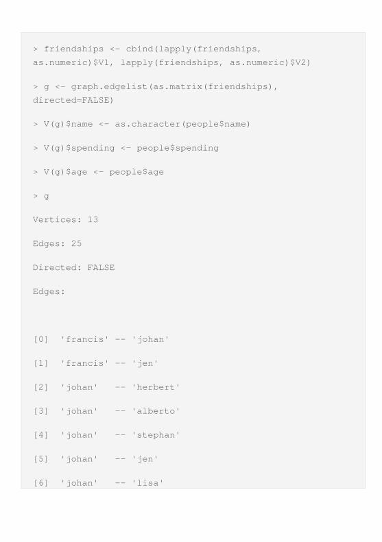
> friendships <- cbind(lapply(friendships,

as.numeric)$V1, lapply(friendships, as.numeric)$V2)

> g <- graph.edgelist(as.matrix(friendships),

directed=FALSE)

> V(g)$name <- as.character(people$name)

> V(g)$spending <- people$spending

> V(g)$age <- people$age

> g

Vertices: 13

Edges: 25

Directed: FALSE

Edges:

[0] 'francis' -- 'johan'

[1] 'francis' -- 'jen'

[2] 'johan' -- 'herbert'

[3] 'johan' -- 'alberto'

[4] 'johan' -- 'stephan'

[5] 'johan' -- 'jen'

[6] 'johan' -- 'lisa'

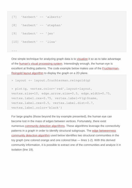
[7] 'herbert' -- 'alberto'

[8] 'herbert' -- 'stephan'

[9] 'herbert' -- 'jen'

[10] 'herbert' -- 'lisa'

...

One simple technique for analyzing graph data is to visualize it so as to take advantage

of the human’s visual processing system. Interestingly enough, the human eye is

excellent at finding patterns. The code example below makes use of the Fruchterman-

Reingold layout algorithm to display the graph on a 2D plane.

> layout <- layout.fruchterman.reingold(g)

> plot(g, vertex.color='red',layout=layout,

vertex.size=10, edge.arrow.size=0.5, edge.width=0.75,

vertex.label.cex=0.75, vertex.label=V(g)$name,

vertex.label.cex=0.5, vertex.label.dist=0.7,

vertex.label.color='black')

For large graphs (those beyond the toy example presented), the human eye can

become lost in the mass of edges between vertices. Fortunately, there exist

numerous community detection algorithms. These algorithms leverage the connectivity

patterns in a graph in order to identify structural subgroups. The edge betweenness

community detection algorithm used below identifies two structural communities in the

toy graph (one colored orange and one colored blue — lines 1-2). With this derived

community information, it is possible to extract one of the communities and analyze it in

isolation (line 19).

> V(g)$community = community.to.membership(g,

edge.betweenness.community(g)$merges,

steps=11)$membership+1

> data.frame(name=V(g)$name, community=V(g)$community)

name community

1 francis 1

2 johan 1

3 herbert 1

4 mike 2

5 richard 2

6 alberto 1

7 stephan 1

8 dan 2

9 jen 1

10 john 2

11 matt 2

12 lisa 1

13 ariana 1

> color <- c(colors()[631], colors()[498])

> plot(g,

vertex.color=color[V(g)$community],layout=layout,

vertex.size=10, edge.arrow.size=0.5, edge.width=0.75,

vertex.label.cex=0.75, vertex.label=V(g)$name,

vertex.label.cex=0.5, vertex.label.dist=0.7,

vertex.label.color='black')

> h <- delete.vertices(g, V(g)[V(g)$community == 2])

> plot(h,

vertex.color="red",layout=layout.fruchterman.reingold,

vertex.size=10, edge.arrow.size=0.5, edge.width=0.75,

vertex.label.cex=0.75, vertex.label=V(h)$name,

vertex.label.cex=0.5, vertex.label.dist=0.7,

vertex.label.color='black')

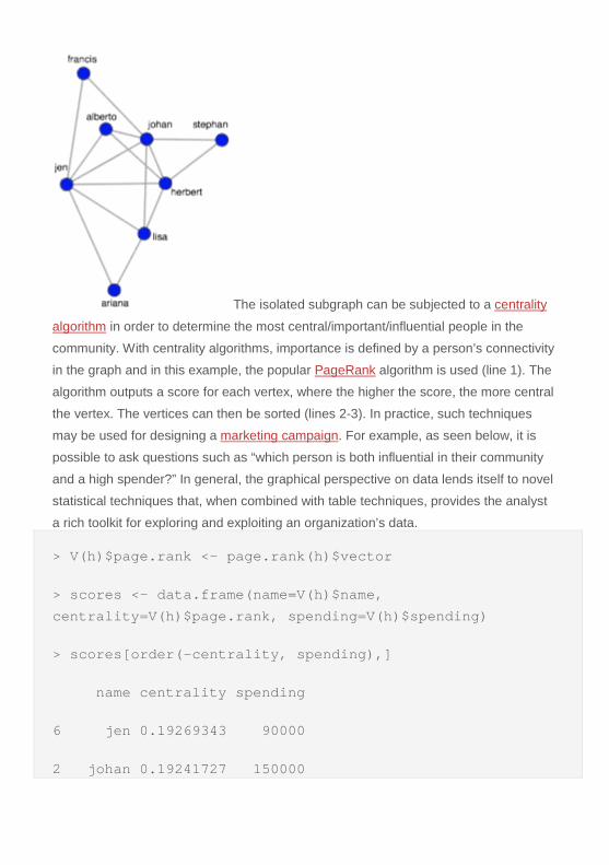
The isolated subgraph can be subjected to a centrality

algorithm in order to determine the most central/important/influential people in the

community. With centrality algorithms, importance is defined by a person’s connectivity

in the graph and in this example, the popular PageRank algorithm is used (line 1). The

algorithm outputs a score for each vertex, where the higher the score, the more central

the vertex. The vertices can then be sorted (lines 2-3). In practice, such techniques

may be used for designing a marketing campaign. For example, as seen below, it is

possible to ask questions such as “which person is both influential in their community

and a high spender?” In general, the graphical perspective on data lends itself to novel

statistical techniques that, when combined with table techniques, provides the analyst

a rich toolkit for exploring and exploiting an organization’s data.

> V(h)$page.rank <- page.rank(h)$vector

> scores <- data.frame(name=V(h)$name,

centrality=V(h)$page.rank, spending=V(h)$spending)

> scores[order(-centrality, spending),]

name centrality spending

6 jen 0.19269343 90000

2 johan 0.19241727 150000

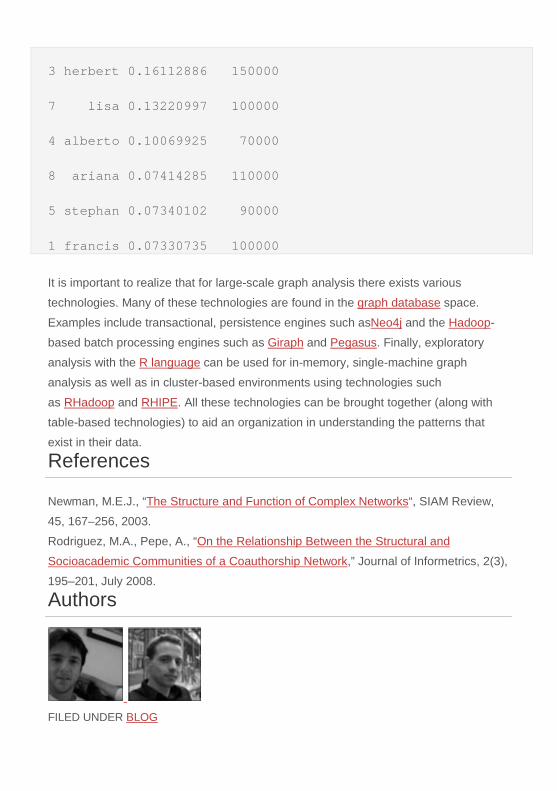
3 herbert 0.16112886 150000

7 lisa 0.13220997 100000

4 alberto 0.10069925 70000

8 ariana 0.07414285 110000

5 stephan 0.07340102 90000

1 francis 0.07330735 100000

It is important to realize that for large-scale graph analysis there exists various

technologies. Many of these technologies are found in the graph database space.

Examples include transactional, persistence engines such asNeo4j and the Hadoop-

based batch processing engines such as Giraph and Pegasus. Finally, exploratory

analysis with the R language can be used for in-memory, single-machine graph

analysis as well as in cluster-based environments using technologies such

as RHadoop and RHIPE. All these technologies can be brought together (along with

table-based technologies) to aid an organization in understanding the patterns that

exist in their data.

References

Newman, M.E.J., “The Structure and Function of Complex Networks“, SIAM Review,

45, 167–256, 2003.

Rodriguez, M.A., Pepe, A., “On the Relationship Between the Structural and

Socioacademic Communities of a Coauthorship Network,” Journal of Informetrics, 2(3),

195–201, July 2008.

Authors

FILED UNDER BLOG

Graph Degree Distributions using R over Hadoop

FEBRUARY 5, 2012 1 COMMENT

There are two common types of graph engines. One type is focused on providing real-

time, traversal-based algorithms over linked-list graphs represented on a single-server.

Such engines are typically called graph databases and some of the vendors

include Neo4j, OrientDB, DEX, and InfiniteGraph. The other type of graph engine is

focused on batch-processing using vertex-centric message passing within a graph

represented across a cluster of machines. Graph engines of this form

include Hama, Golden Orb, Giraph, and Pregel.

The purpose of this post is to demonstrate how to express the computation of two

fundamental graph statistics — each as a graph traversal and as

a MapReduce algorithm. The graph engines explored for this purpose are Neo4j

and Hadoop. However, with respects to Hadoop, instead of focusing on a particular

vertex-centric BSP-based graph-processing package such as Hama or Giraph, the

results presented are via native Hadoop (HDFS + MapReduce). Moreover, instead of

developing the MapReduce algorithms in Java, the R programming language is

used. RHadoop is a small, open-source package developed by Revolution

Analytics that binds R to Hadoop and allows for the representation of MapReduce

algorithms using native R. The two graph algorithms presented compute degree statistics: vertex in-

degree and graph in-degree distribution. Both are related, and in fact, the results of the

first can be used as the input to the second. That is, graph in-degree distribution is a

function of vertex in-degree. Together, these two fundamental statistics serve as a

foundation for more quantifying statistics developed in the domains of graph

theory and network science. 1. Vertex in-degree: How many incoming edges does vertex X have?

2. Graph in-degree distribution: How many vertices have X number of

incoming edges?

These two algorithms are calculated over an

artificially generated graph that contains 100,000 vertices and 704,002 edges. A subset

is diagrammed on the left. The algorithm used to generate the graph is

called preferential attachment. Preferential attachment yields graphs with “natural

statistics” that have degree distributions that are analogous to real-world

graphs/networks. The respective iGraph R code is provided below. Once constructed

and simplified (i.e. no more than one edge between any two vertices and no self-

loops), the vertices and edges are counted. Next, the first five edges are iterated and

displayed. The first edge reads, “vertex 2 is connected to vertex 0.” Finally, the graph is

persisted to disk as a GraphML file.

~$ r

R version 2.13.1 (2011-07-08)

Copyright (C) 2011 The R Foundation for Statistical

Computing

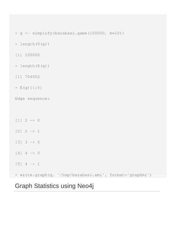
> g <- simplify(barabasi.game(100000, m=10))

> length(V(g))

[1] 100000

> length(E(g))

[1] 704002

> E(g)[1:5]

Edge sequence:

[1] 2 -> 0

[2] 2 -> 1

[3] 3 -> 0

[4] 4 -> 0

[5] 4 -> 1

> write.graph(g, '/tmp/barabasi.xml', format='graphml')

Graph Statistics using Neo4j

When a graph is on the

order of 10 billion elements (vertices+edges), then a single-server graph database is

sufficient for performing graph analytics. As a side note, when those

analytics/algorithms are “ego-centric” (i.e. when the traversal emanates from a single

vertex or small set of vertices), then they can typically be evaluated in real-time (e.g. <

1000 ms). To compute these in-degree statistics, Gremlin is used. Gremlin is a graph

traversal language developed by TinkerPop that is distributed with Neo4j, OrientDB,

DEX, InfiniteGraph, and the RDF engine Stardog. The Gremlin code below loads the

GraphML file created by R in the previous section into Neo4j. It then performs a count

of the vertices and edges in the graph.

~$ gremlin

\,,,/

(o o)

-----oOOo-(_)-oOOo-----

gremlin> g = new Neo4jGraph('/tmp/barabasi')

==>neo4jgraph[EmbeddedGraphDatabase [/tmp/barabasi]]

gremlin> g.loadGraphML('/tmp/barabasi.xml')

==>null

gremlin> g.V.count()

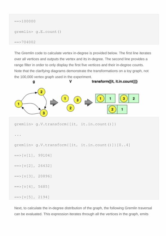
==>100000

gremlin> g.E.count()

==>704002

The Gremlin code to calculate vertex in-degree is provided below. The first line iterates

over all vertices and outputs the vertex and its in-degree. The second line provides a

range filter in order to only display the first five vertices and their in-degree counts.

Note that the clarifying diagrams demonstrate the transformations on a toy graph, not

the 100,000 vertex graph used in the experiment.

gremlin> g.V.transform{[it, it.in.count()]}

...

gremlin> g.V.transform{[it, it.in.count()]}[0..4]

==>[v[1], 99104]

==>[v[2], 26432]

==>[v[3], 20896]

==>[v[4], 5685]

==>[v[5], 2194]

Next, to calculate the in-degree distribution of the graph, the following Gremlin traversal

can be evaluated. This expression iterates through all the vertices in the graph, emits

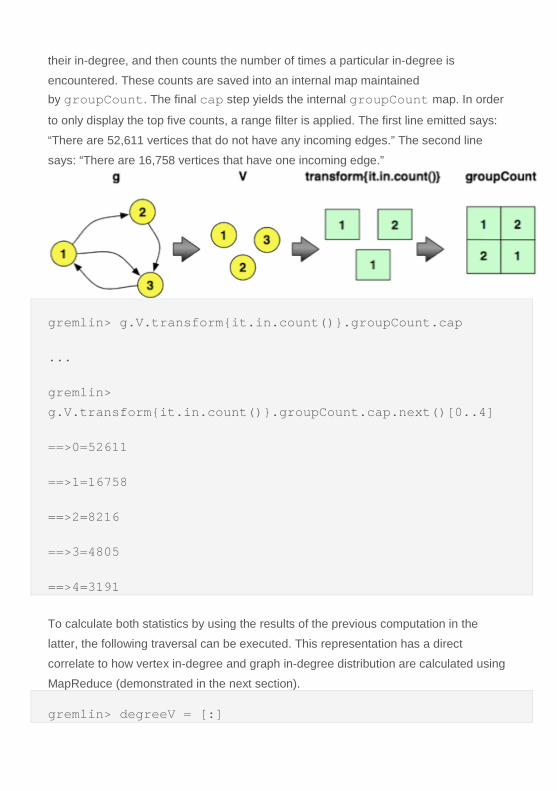
their in-degree, and then counts the number of times a particular in-degree is

encountered. These counts are saved into an internal map maintained by groupCount. The final cap step yields the internal groupCount map. In order

to only display the top five counts, a range filter is applied. The first line emitted says:

“There are 52,611 vertices that do not have any incoming edges.” The second line

says: “There are 16,758 vertices that have one incoming edge.”

gremlin> g.V.transform{it.in.count()}.groupCount.cap

...

gremlin>

g.V.transform{it.in.count()}.groupCount.cap.next()[0..4]

==>0=52611

==>1=16758

==>2=8216

==>3=4805

==>4=3191

To calculate both statistics by using the results of the previous computation in the

latter, the following traversal can be executed. This representation has a direct

correlate to how vertex in-degree and graph in-degree distribution are calculated using

MapReduce (demonstrated in the next section).

gremlin> degreeV = [:]

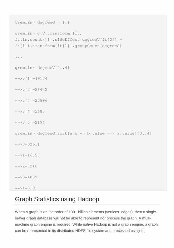
gremlin> degreeG = [:]

gremlin> g.V.transform{[it,

it.in.count()]}.sideEffect{degreeV[it[0]] =

it[1]}.transform{it[1]}.groupCount(degreeG)

...

gremlin> degreeV[0..4]

==>v[1]=99104

==>v[2]=26432

==>v[3]=20896

==>v[4]=5685

==>v[5]=2194

gremlin> degreeG.sort{a,b -> b.value <=> a.value}[0..4]

==>0=52611

==>1=16758

==>2=8216

==>3=4805

==>4=3191

Graph Statistics using Hadoop

When a graph is on the order of 100+ billion elements (vertices+edges), then a single-

server graph database will not be able to represent nor process the graph. A multi-

machine graph engine is required. While native Hadoop is not a graph engine, a graph

can be represented in its distributed HDFS file system and processed using its

distributed processing MapReduce framework. The graph generated previously is

loaded up in R and a count of its vertices and edges is conducted. Next, the graph is

represented as an edge list. An edge list (for a single-relational graph) is a list of pairs,

where each pair is ordered and denotes the tail vertex id and the head vertex id of the

edge. The edge list can be pushed to HDFS using RHadoop. The variable edge.list represents a pointer to this HDFS file.

> g <- read.graph('/tmp/barabasi.xml', format='graphml')

> length(V(g))

[1] 100000

> length(E(g))

[1] 704002

> edge.list <- to.dfs(get.edgelist(g))

In order to calculate vertex in-degree, a MapReduce job is evaluated on edge.list.

The map function is fed key/value pairs where the key is an edge id and the value is

the ids of the tail and head vertices of the edge (represented as a list). For each

key/value input, the head vertex (i.e. incoming vertex) is emitted along with the number

1. The reduce function is fed key/value pairs where the keys are vertices and the

values are a list of 1s. The output of the reduce job is a vertex id and the length of the

list of 1s (i.e. the number of times that vertex was seen as an incoming/head vertex of

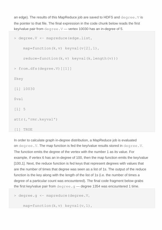
an edge). The results of this MapReduce job are saved to HDFS and degree.V is

the pointer to that file. The final expression in the code chunk below reads the first key/value pair from degree.V — vertex 10030 has an in-degree of 5.

> degree.V <- mapreduce(edge.list,

map=function(k,v) keyval(v[2],1),

reduce=function(k,v) keyval(k,length(v)))

> from.dfs(degree.V)[[1]]

$key

[1] 10030

$val

[1] 5

attr(,"rmr.keyval")

[1] TRUE

In order to calculate graph in-degree distribution, a MapReduce job is evaluated on degree.V. The map function is fed the key/value results stored in degree.V.

The function emits the degree of the vertex with the number 1 as its value. For

example, if vertex 6 has an in-degree of 100, then the map function emits the key/value

[100,1]. Next, the reduce function is fed keys that represent degrees with values that

are the number of times that degree was seen as a list of 1s. The output of the reduce

function is the key along with the length of the list of 1s (i.e. the number of times a

degree of a particular count was encountered). The final code fragment below grabs the first key/value pair from degree.g — degree 1354 was encountered 1 time.

> degree.g <- mapreduce(degree.V,

map=function(k,v) keyval(v,1),

reduce=function(k,v) keyval(k,length(v)))

> from.dfs(degree.g)[[1]]

$key

[1] 1354

$val

[1] 1

attr(,"rmr.keyval")

[1] TRUE

In concert, these two computations can be composed into a single MapReduce

expression.

> degree.g <- mapreduce(mapreduce(edge.list,

map=function(k,v) keyval(v[2],1),

reduce=function(k,v) keyval(k,length(v))),

map=function(k,v) keyval(v,1),

reduce=function(k,v) keyval(k,length(v)))

Note that while a graph can be on the order of 100+ billion elements, the degree distribution is much smaller and can typically fit into memory. In general, edge.list

> degree.V > degree.g. Due to this fact, it is possible to pull

the degree.g file off of HDFS, place it into main memory, and plot the results stored

within. The degree.gdistribution is plotted on a log/log plot. As suspected, the

preferential attachment algorithm generated a graph with natural “scale-free” statistics

— most vertices have a small in-degree and very few have a large in-degree.

> degree.g.memory <- from.dfs(degree.g)

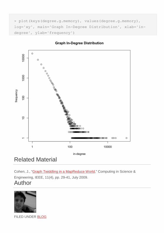
> plot(keys(degree.g.memory), values(degree.g.memory),

log='xy', main='Graph In-Degree Distribution', xlab='in-

degree', ylab='frequency')

Related Material

Cohen, J., “Graph Twiddling in a MapReduce World,” Computing in Science &

Engineering, IEEE, 11(4), pp. 29-41, July 2009.

Author

FILED UNDER BLOG

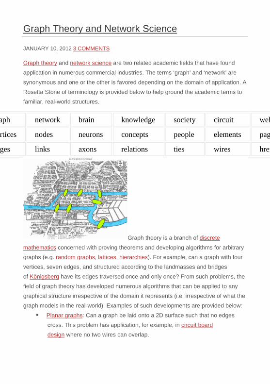
Graph Theory and Network Science

JANUARY 10, 2012 3 COMMENTS

Graph theory and network science are two related academic fields that have found

application in numerous commercial industries. The terms ‘graph’ and ‘network’ are

synonymous and one or the other is favored depending on the domain of application. A

Rosetta Stone of terminology is provided below to help ground the academic terms to

familiar, real-world structures.

aph network brain knowledge society circuit web

rtices nodes neurons concepts people elements pag

ges links axons relations ties wires href

Graph theory is a branch of discrete

mathematics concerned with proving theorems and developing algorithms for arbitrary

graphs (e.g. random graphs, lattices, hierarchies). For example, can a graph with four

vertices, seven edges, and structured according to the landmasses and bridges

of Königsberg have its edges traversed once and only once? From such problems, the

field of graph theory has developed numerous algorithms that can be applied to any

graphical structure irrespective of the domain it represents (i.e. irrespective of what the

graph models in the real-world). Examples of such developments are provided below:

Planar graphs: Can a graph be laid onto a 2D surface such that no edges

cross. This problem has application, for example, in circuit board

design where no two wires can overlap.

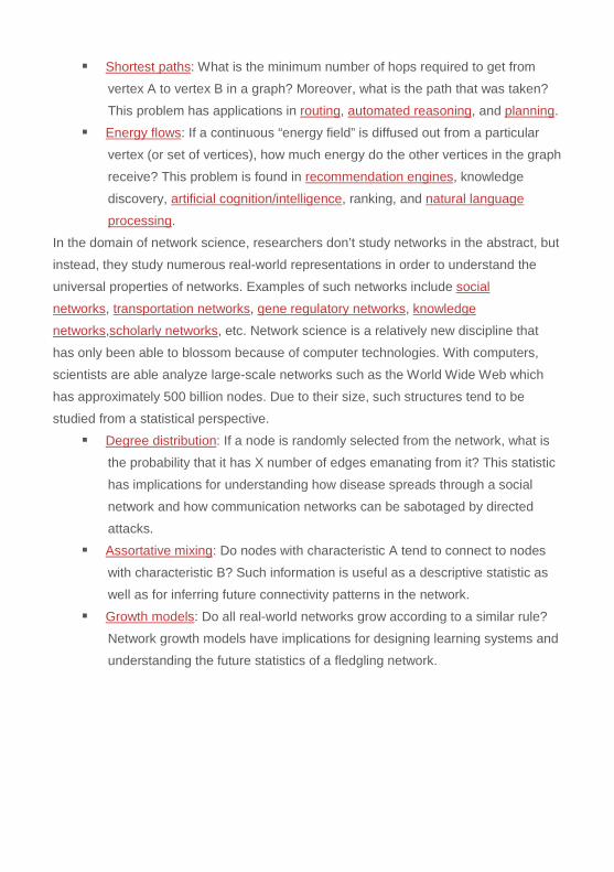
Shortest paths: What is the minimum number of hops required to get from

vertex A to vertex B in a graph? Moreover, what is the path that was taken?

This problem has applications in routing, automated reasoning, and planning.

Energy flows: If a continuous “energy field” is diffused out from a particular

vertex (or set of vertices), how much energy do the other vertices in the graph

receive? This problem is found in recommendation engines, knowledge

discovery, artificial cognition/intelligence, ranking, and natural language

processing.

In the domain of network science, researchers don’t study networks in the abstract, but

instead, they study numerous real-world representations in order to understand the

universal properties of networks. Examples of such networks include social

networks, transportation networks, gene regulatory networks, knowledge

networks,scholarly networks, etc. Network science is a relatively new discipline that

has only been able to blossom because of computer technologies. With computers,

scientists are able analyze large-scale networks such as the World Wide Web which

has approximately 500 billion nodes. Due to their size, such structures tend to be

studied from a statistical perspective.

Degree distribution: If a node is randomly selected from the network, what is

the probability that it has X number of edges emanating from it? This statistic

has implications for understanding how disease spreads through a social

network and how communication networks can be sabotaged by directed

attacks.

Assortative mixing: Do nodes with characteristic A tend to connect to nodes

with characteristic B? Such information is useful as a descriptive statistic as

well as for inferring future connectivity patterns in the network.

Growth models: Do all real-world networks grow according to a similar rule?

Network growth models have implications for designing learning systems and

understanding the future statistics of a fledgling network.

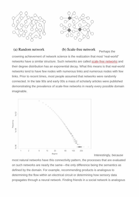
Perhaps the

crowning achievement of network science is the realization that most “real-world”

networks have a similar structure. Such networks are called scale-free networks and

their degree distribution has an exponential decay. What this means is that real-world

networks tend to have few nodes with numerous links and numerous nodes with few

links. Prior to recent times, most people assumed that networks were randomly

connected. In the late 90s and early 00s a mass of scholarly articles were published

demonstrating the prevalence of scale-free networks in nearly every possible domain

imaginable.

Interestingly, because

most natural networks have this connectivity pattern, the processes that are evaluated

on such networks are nearly the same—the only difference being the semantics as

defined by the domain. For example, recommending products is analogous to

determining the flow within an electrical circuit or determining how sensory data

propagates through a neural network. Finding friends in a social network is analogous

to routing packets in a communication network or determining the shortest route on a

transportation network. Ranking web pages is analogous to determining the most

influential people in a social network or finding the most relevant concepts in a

knowledge network. Finally, all these problems are variations of one general process—

graph traversing. Graph traversing is the simple process of moving from one vertex to

another vertex over the edges in the graph and either mutating the structure or

collecting bits of information along the way. The result of a traversal is either an

evolution of the graph or a statistic about the graph.

The tools and techniques developed by graph theorists and networks scientists has an

astounding number of practical applications. Interestingly enough, once one has a

general understanding of graph theory and network science, the world’s problems start

to be seen as one in the same problem.

Related Material

Rodriguez, M.A., Neubauer, P., “The Graph Traversal Pattern,” Graph Data

Management: Techniques and Applications, eds. S. Sakr, E. Pardede, IGI Global,

ISBN:9781613500538, August 2011.

Watkins, J.H., M.A. Rodriguez, “A Survey of Web-based Collective Decision Making

Systems,” Studies in Computational Intelligence: Evolution of the Web in Artificial

Intelligence Environments, Springer-Verlag, pages 245-279, 2008.

Rodriguez, M.A., “A Graph-Based Movie Recommender Engine,” Marko A. Rodriguez

Blog, 2011.

Rodriguez, M.A., “Graphs, Brains, and Gremlin,” Marko A. Rodriguez Blog, 2011.

Authors

FILED UNDER BLOG