Fatigue Crack Propagation of Multiple

Coplanar Cracks with the Coupled Extended

Finite Element/Fast Marching Method

D. L. Chopp a,∗,1 and N. Sukumar b

aEngineering Sciences and Applied Mathematics Dept., Northwestern University,Evanston, IL 60208-3125

bDepartment of Civil and Environmental Engineering, University of California,Davis, CA 95616

Abstract

A numerical technique for modeling fatigue crack propagation of multiple coplanarcracks is presented. The proposed method couples the Extended Finite ElementMethod (X-FEM) [40] to the Fast Marching Method (FMM) [34]. The entire crackgeometry, including one or more cracks, is represented by a single signed distance(level set) function. Merging of distinct cracks is handled naturally by the fastmarching method with no collision detection or mesh reconstruction required. Thefast marching method in conjunction with the Paris crack growth law is used toadvance the crack front. In the X-FEM, a discontinuous function and the two-dimensional asymptotic crack-tip displacement fields are added to the finite elementapproximation to account for the crack using the notion of partition of unity [20].This enables the domain to be modeled by a single fixed finite element mesh withno explicit meshing of the crack surfaces. In an earlier study [39], the methodology,algorithm, and implementation for three-dimensional crack propagation of singlecracks was introduced. In this paper, simulations for multiple planar cracks arepresented, with crack merging and fatigue growth carried out without any user-intervention or remeshing.

Key words: partition of unity, extended finite element method, fast marchingmethod, level set method, fatigue crack growth, coplanar cracks in 3-d

∗ Corresponding author.Email address: chopp@northwestern.edu (D. L. Chopp).

1 This work was supported in part by the NSF/DARPA VIP program under awardsDMS-9615877 and NSF DMS-9872036

Preprint submitted to Elsevier Science 25 October 2002

1 Introduction

Numerical methods for capturing moving interfaces have played a vital rolein a broad range of modeling applications from multi-phase fluid flow to thin-film deposition and etching. In many of these applications, solution of anelliptic equation involving irregularly shaped moving boundaries is requiredin order to obtain the velocity field of the interface. Many different techniquesare available, each with their own strengths and weaknesses making no singletechnique optimal for all moving interface problems.

In this paper, we present a recently developed numerical method, which hasa different set of strengths than existing methods. It is the result of cou-pling a popular interface capturing method, the fast marching method (FMM)[32,33,8], with an extended form of the classical finite element method, theExtended Finite Element Method (X-FEM) [22,40]. The two methods forma natural partnership for capturing a monotonically advancing front whichrequires a coupled elliptic equation solution for determining the front velocity.In the FMM, the motion of the interface is embedded in the solution ϕ of astatic Hamilton-Jacobi equation which describes the position of the interfaceat time t by the level contour ϕ(x) = t. This function ϕ is computed usinga single pass through the mesh by carefully selecting the order in which thenodal values are evaluated. In the X-FEM, additional non-linear functionsare added to the finite element approximation to account for the interfaceusing the notion of partition of unity. This enables the domain to be mod-eled by finite elements with no explicit meshing of the crack surfaces. In thecoupled method, the FMM maintains the location and motion of the crackfront whereas the X-FEM is used to compute the local front velocity. For atreatment of non-monotonically advancing fronts, the fast marching methodis replaced by the level set method [28], see [19].

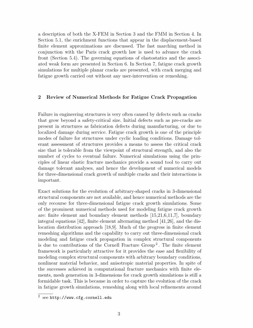
In [39], Sukumar and co-workers applied this algorithm to single planar three-dimensional fatigue cracks. In that paper, the accuracy of the SIF calculations,as well as the algorithm as a whole, tested favorably against the known solutionof a single circular penny crack embedded in an infinite domain. A sample ofthe results are shown in Fig. 1. However, that algorithm was not able to handlemultiple cracks which may merge as they grow. The ease with which the fastmarching method can handle merging interfaces is one of its strongest features,but difficulties remain in the corresponding implementation of the X-FEM. Atissue is how to properly employ the X-FEM when separate interfaces, such asdistinct cracks, approach each other.

In this paper, we give an overview of the original method, then describe howto incorporate multiple cracks which are able to coalesce. We begin by de-scribing existing numerical methods for modeling fatigue cracks and then give

2

a description of both the X-FEM in Section 3 and the FMM in Section 4. InSection 5.1, the enrichment functions that appear in the displacement-basedfinite element approximations are discussed. The fast marching method inconjunction with the Paris crack growth law is used to advance the crackfront (Section 5.4). The governing equations of elastostatics and the associ-ated weak form are presented in Section 6. In Section 7, fatigue crack growthsimulations for multiple planar cracks are presented, with crack merging andfatigue growth carried out without any user-intervention or remeshing.

2 Review of Numerical Methods for Fatigue Crack Propagation

Failure in engineering structures is very often caused by defects such as cracksthat grow beyond a safety-critical size. Initial defects such as pre-cracks arepresent in structures as fabrication defects during manufacturing, or due tolocalized damage during service. Fatigue crack growth is one of the principlemodes of failure for structures under cyclic loading conditions. Damage tol-erant assessment of structures provides a means to assess the critical cracksize that is tolerable from the viewpoint of structural strength, and also thenumber of cycles to eventual failure. Numerical simulations using the prin-ciples of linear elastic fracture mechanics provide a sound tool to carry outdamage tolerant analyses, and hence the development of numerical modelsfor three-dimensional crack growth of multiple cracks and their interactions isimportant.

Exact solutions for the evolution of arbitrary-shaped cracks in 3-dimensionalstructural components are not available, and hence numerical methods are theonly recourse for three-dimensional fatigue crack growth simulations. Someof the prominent numerical methods used for modeling fatigue crack growthare: finite element and boundary element methods [15,21,6,11,7], boundaryintegral equations [42], finite element alternating method [41,26], and the dis-location distribution approach [18,9]. Much of the progress in finite elementremeshing algorithms and the capability to carry out three-dimensional crackmodeling and fatigue crack propagation in complex structural componentsis due to contributions of the Cornell Fracture Group 2 . The finite elementframework is particularly attractive for it provides the ease and flexibility ofmodeling complex structural components with arbitrary boundary conditions,nonlinear material behavior, and anisotropic material properties. In spite ofthe successes achieved in computational fracture mechanics with finite ele-ments, mesh generation in 3-dimensions for crack growth simulations is still aformidable task. This is because in order to capture the evolution of the crackin fatigue growth simulations, remeshing along with local refinements around

2 see http://www.cfg.cornell.edu

3

the crack front are required to obtain accurate solutions for fracture parame-ters such as the stress intensity factor (SIF). Hence, a computational methodthat can automate three-dimensional crack propagation simulations on rela-tively coarse meshes without the need for remeshing or user-intervention isof significance. The use of the FMM with the X-FEM removes the need torepresent and maintain the geometry of the crack at every step, which is aburden in most existing numerical methods for fracture modeling.

The first three-dimensional crack modeling study using the X-FEM [40] dis-cussed the computational geometric issues for the representation of the cracksurface and its interaction with the finite element mesh for the enrichment.In [39], the methodology for crack propagation of single cracks was presented.That basic algorithm coupled with the work in [35] has led to 3-dimensionalnon-planar crack growth in [17]. This advance points to the promise and po-tential of the X-FEM towards the automated modeling of arbitrary crackpropagation in 3-dimensional structural components.

3 Extended Finite Element Method

The Extended Finite Element Method (X-FEM) [22,10,40] is a numericalmethod to model internal (or external) boundaries such as holes, inclusions,or cracks, without requiring the mesh to conform to these boundaries. TheX-FEM is based on a standard Galerkin procedure, and uses the concept ofpartition of unity [20] to accommodate the internal boundaries in the discretemodel. The partition of unity method [20] generalized finite element approx-imations by presenting a means to embed local solutions of boundary-valueproblems into the finite element approximation. This idea was exploited byOden and co-workers [27,12] for problems with internal boundaries—the nu-merical technique was referred to as the Generalized Finite Element Method(GFEM). Stroubolis and co-workers [36,37] have used the partition of unityframework to model holes and cracks in 2-dimensions, whereas Duarte and co-workers [13] have studied the simulation of three-dimensional dynamic crackpropagation.

Partition of unity enrichment for discontinuities and near-tip crack fields wasintroduced in [5]. The displacement enrichment functions for crack problemsare functions that span the asymptotic near-tip displacement field—see [14]for their use in the Element-Free Galerkin method. A significant improvementin discrete 2-dimensional crack growth modeling without the need for anyremeshing strategy was conceived by Moes and co-workers [22], with furtherdevelopments in [10] for holes and branched cracks. The generalized Heavisidestep function was proposed as a means to model the crack away from the crack-tip, with simple rules for the introduction of the discontinuous and crack-tip

4

enrichments. The extension of the X-FEM to 3-dimensional crack problemswas presented in [40]. This advance clearly provided a robust and accuratecomputational tool for modeling discontinuities independent of the mesh ge-ometry. The X-FEM has been successfully applied to quasi-static and fatiguecrack propagation in 2-dimensions [22,10] and 3-dimensions [40,39,23,17]. Thecoupling of level sets with the X-FEM for the description and evolution ofcracks has also been explored in 2-dimensions [35].

The enrichment of the finite element approximation is described as follows.Consider a point x of Rd (d = 1, 2, 3) that lies inside a finite element e.Denote the nodal set N = n1, n2, . . . , nm, where m is the number of nodesof element e. (m = 2 for a linear one-dimensional finite element, m = 3 fora constant-strain triangle, m = 8 for a trilinear hexahedral element, etc.)The enriched displacement approximation for a vector-valued function u(x) :R

d → Rd assumes the form:

uh(x) =∑I

nI∈N

φI(x)uI

︸ ︷︷ ︸classical

+∑J

nJ∈Ng

φJ(x)ψ(x)aJ

︸ ︷︷ ︸enriched

, (uI , aJ ∈ Rd) (1)

where the nodal set Ng is defined as:

Ng = nJ : nJ ∈ N, ωJ ∩ Ωg = ∅. (2)

In the above equation, ωJ = supp(nJ) is the support of the nodal shapefunction φJ(x), which consists of the union of all elements with nJ as one ofits vertices, or in other words the union of elements in which φJ(x) is non-zero. In addition, Ωg is the domain associated with a geometric entity such ascrack-tip [22], crack surface in 3-dimensions [40], or material interface [38]. Ingeneral, the choice of the enrichment function ψ(x) that appears in Eq. (1)depends on the geometric entity.

4 Fast Marching Method

The Fast Marching Method was first introduced by Sethian [32], and laterimproved by Sethian [33] and Chopp [8]. The method computes the crossingtime map for a monotonically advancing front in an arbitrary number of spatialdimensions. The crossing time map is constructed by solving an equation ofthe form

‖∇ϕ(x)‖ =1

F (x), (3)

where F (x) is the front speed at the point x and ϕ(x) is the time at whichthe evolving front passes through the point x. The initial front is then givenby ϕ−1(0), and the level contour ϕ−1(t) is the location of the front at time t.

5

The solution of Eq. (3) is constructed by first replacing the gradient by suitableupwind operators, and then systematically advancing the front by marchingoutwards from the boundary data in an upwind fashion. For N nodes, themethod has a total operation count of O(N logN). If F (x) ≡ 1, then Eq. (3)becomes the Eikonal equation and the solution ϕ(x) of Eq. (3) gives the dis-tance from x to the zero contour ϕ−1(0). In this paper, we use this applicationto compute the distance map from the grid nodes to the crack front.

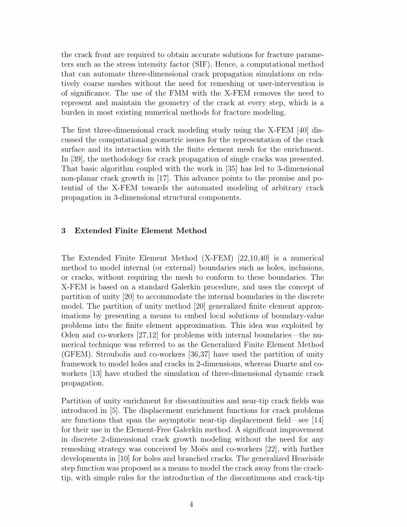
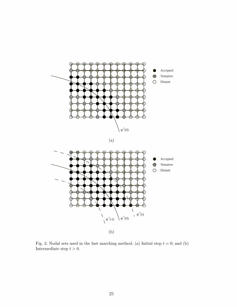
In the FMM, all the nodes in the mesh are sorted into three disjoint sets, theset of all accepted nodes A, the set of all tentative nodes T , and the set of alldistant nodes D. The method systematically moves nodes from the set D tothe set T and finally into the set A and terminates when all nodes are in theset A. Briefly, the set A consists of all nodes x whose value of ϕ(x) has beencomputed, the set T consists of all nodes that are candidates for inclusion intothe set A, and the set D consists of all nodes which are too far from the set Ato be candidates. With these sets in mind and denoting xi,j as the coordinateof node (i, j) and ϕi,j ≡ ϕ(xi,j), the algorithm proceeds as follows:

(1) Initialize a core set of nodes to be in the set A. The value of ϕ(x) for x ∈ Ais determined by direct computation. Each element of the mesh throughwhich the zero contour of ϕ crosses, i.e. the initial front position, has eachof its nodes start in the set A and the value of each node is determinedby directly computing the distance from each node to the level contourin the element. We use bicubic interpolation on the rectilinear FMM gridto approximate the contour. A variant of Newton’s method is used tocompute the distance to that contour. For additional details, see Chopp[8].

(2) For each node x ∈ A, each neighboring node y /∈ A connected to x isassigned a tentative value ϕ(y) and placed in the set T . The tentativevalue is constructed by using second-order one-sided finite difference ap-proximations for Eq. (3). For example, if we wish to compute ϕi,j withxi−1,j, xi,j+1 ∈ A, then ϕi,j is constructed by solving

[max

(D−

x ϕi,j +s−1 ∆x

2D−

x D−x ϕi,j,−D+

x ϕi,j +s+1 ∆x

2D+

x D+x ϕi,j, 0

)]2

+

[max

(D−

y ϕi,j +s−2 ∆y

2D−

y D−y ϕi,j,−D+

y ϕi,j +s+2 ∆y

2D+

y D+y ϕi,j, 0

)]2

= 1/F 2i,j. (4)

where

D−x ϕi,j =

ϕi,j − ϕi−1,j

∆x, D+

x ϕi,j =ϕi+1,j − ϕi,j

∆x, (5)

and

s−1 =

1 xi−1,j ∈ A

0 xi−1,j /∈ A, s+

1 =

1 xi+1,j ∈ A

0 xi+1,j /∈ A. (6)

6

Expressions for D−y , D+

y , s−2 , s+2 are similar (see [33]). Equation (4) is

actually a quadratic in the unknown quantity ϕi,j and can be solved toproduce two possible values. The larger of the two solutions is taken forϕi,j. The set T is maintained as a sorted list by a heap sort method withthe smallest value always at the top.

Pictorially, the set A now consists of all nodes immediately adjacentto the zero contour ϕ−1(0), the set T is a thin layer of nodes surroundingthe nodes in A, and the set D is everything else (Fig. 2).

(3) The main loop now begins by taking the node x ∈ T with the smallestvalue for ϕ(x) and moves it from the set T to the set A.

(4) Each node y adjacent to the node x selected in step 3, and not alreadyin A, has its value ϕ(y) updated using Eq. (4). If y ∈ T , then T must bere-sorted to account for the changed value of ϕ(y). If y ∈ D, it is movedfrom D to T .

(5) If T = ∅, then go to step 3

For further information regarding the fast marching method and the level setmethod, see [34].

5 Three-Dimensional Crack Modeling

The merits of coupling level sets to the extended finite element method wasfirst explored in [38] to model static material interfaces, and subsequently itsadvantages further realized in [39,35,23,17] for modeling crack discontinuities.The advantages that accrue by using the level set framework in the X-FEMare the following:

(1) Level sets provide greater ease and simplification in the representationof geometric entities such as holes, inclusions (material interfaces) andcracks, which are typically encountered in solid mechanics applications.Instead of a simplex or Bezier surface representation of the geometry,now a simple function-representation (level set ϕ) is used, which requiresonly the storage of signed distance values at discrete points (nodes) withfinite element interpolation used to obtain the value of the level set atany point in the domain.

(2) Geometric computations for the crack in relation to the finite elementmesh as well as geometric properties of the crack front (such as normaland tangent vectors) are readily computed knowing the level set function[39].

(3) The selection of nodes to be enriched and the computation of the enrich-ment functions for crack problems [39,35] or material interfaces [38,19]use the level set function(s).

(4) For crack modeling in 3-dimensions, the level sets also provide a means to

7

easily compute the local orthogonal crack front coordinate system thatis required for stress intensity factor computations using domain inte-gral representations [39,23,17]. This task is presently carried out usingNewton’s method (iterative procedure) in 3-dimensional fracture compu-tations using finite element techniques [16].

Geometric issues associated with the representation of the crack surface, theevolution of the crack front, and the merging of multiple cracks, are all re-solved by using level set (signed distance) functions and the fast marchingmethod. All the cracks are represented by a single two-dimensional signed dis-tance function corresponding to the crack plane. In the X-FEM, each crack ismodeled by enriching the nodes whose nodal shape function supports inter-sect the interior of the crack. The selection of nodes for enrichment as well asthe computation of enrichment functions is carried out using signed distancefunctions. In addition to the above, partitioning algorithms are also imple-mented if the crack intersects the finite elements—see [40] for details. In thefollowing, we restrict the description of the implementation to planar cracks(x1-x2 plane) in three dimensions.

5.1 Enrichment Functions

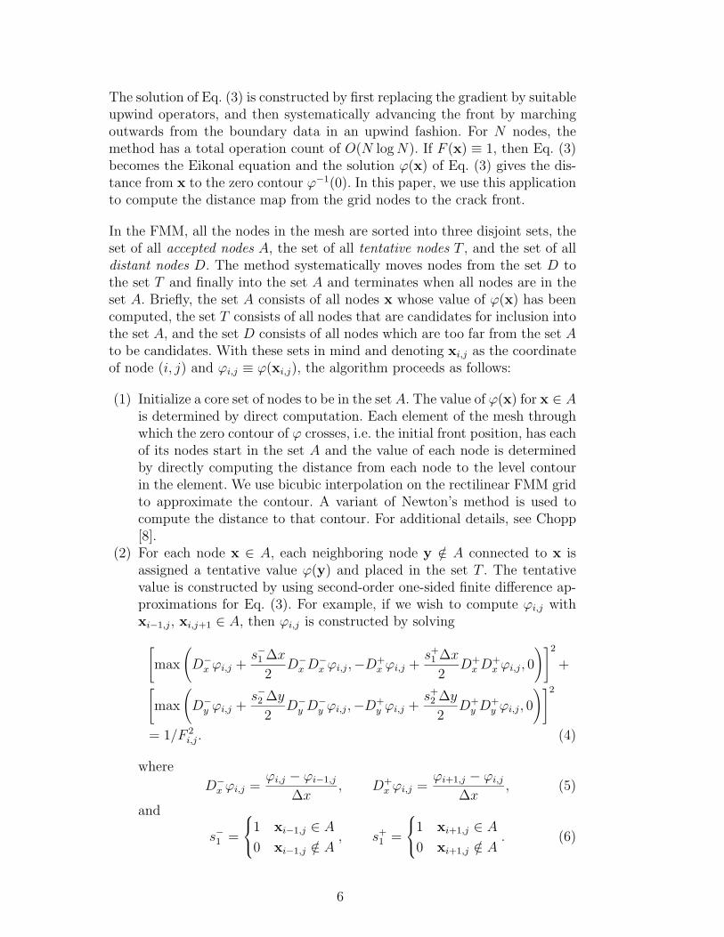
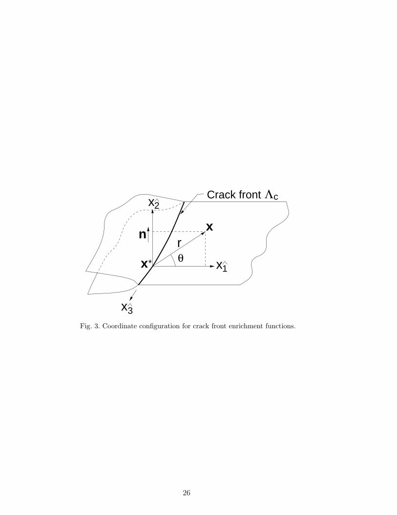
Consider a single crack in 3-dimensions, and let Γc be the crack surface andΛc the crack front. Note that for an internal crack, the crack front correspondsto the boundary of the crack: Λc = ∂Γc whereas for an edge crack, the crackfront is only part of the boundary: Λc ⊂ ∂Γc. The interior of a planar crack ismodeled by the enrichment function H(x), which we refer to as a generalizedHeaviside step function. The function H(x) takes on the value +1 above thecrack and −1 below the crack. More precisely, let x∗ be the closest point to xon the crack Γc, and n be the normal to the crack plane (Fig. 3). The H(x)function is then given by

H(x) =

1 if (x− x∗) · n ≥ 0

−1 otherwise. (7)

In the neighborhood of the crack front, the asymptotic fields are two-dimensionalin nature, and enrichment functions which incorporate the radial and angularbehavior of the asymptotic near-tip displacement field are used. The crack-front enrichment functions are:

Φ(x) ≡ ψ1, ψ2, ψ3, ψ4 =

[√r cos

θ

2,√

r sinθ

2,√

r sin θ sinθ

2,√

r sin θ cosθ

2

],

(8)

8

where r and θ are polar coordinates in the x1-x2 plane (Fig. 3). Note that thesecond function in the above equation is discontinuous on the crack plane.

At any point x, let xp be the orthogonal projection of x onto the crack plane.Next, the signed distance function ϕ1 represents the crack geometry, so ϕ1(x)is the signed distance from xp to the crack front. Also define ϕ2(x) to be thesigned height of x above or below the crack plane. Therefore, at a point x, forwhich the crack front enrichment functions are to be computed, x1 = ϕ1(xp),and x2 = ϕ2(x) [39]. Using the above, the enrichment functions Eq. (7), Eq. (8)can be computed from

r =√

x21+ x2

2=

√(ϕ1(xp))2 + (ϕ2(x))2, (9)

θ = tan−1(x2/x1) = tan−1(ϕ2(x)/ϕ1(xp)), (10)

H(x) = sign(ϕ2(x)) =

1 if ϕ2(x) ≥ 0

−1 otherwise. (11)

The use of the crack-front enrichment functions serves two main purposes:

(1) sub-mesh resolution of the crack-front location; and(2) better accuracy on relatively coarse finite element meshes [22,40].

5.2 Selection of Enriched Nodes

We next describe the enrichment for 3-dimensional crack modeling. The en-riched finite element approximation is [40]:

uh(x) =∑I

nI∈N

φI(x)uI +∑J

nJ∈Nc

φJ(x)H(x)aJ +∑K

nK∈Nf

φK(x)

(4∑

l=1

ψl(x)blK

).

(12)The second and third terms on the right-hand side of the above equation arethe discontinuity and front enrichments, respectively. The set Nf consists ofthose nodes for which the closure of the nodal shape function support intersectsthe crack front. The set Nc is the set of nodes whose nodal shape functionsupport is intersected by the crack and which do not belong to Nf :

Nf = nK : nK ∈ N, ωK ∩ Λc = ∅, (13)

Nc = nJ : nJ ∈ N, ωJ ∩ Γc = ∅, nJ ∈ Nf. (14)

By using the sign of the level set (signed distance) functions ϕ1 and ϕ2 (seeSection 5.1), the nodal setsNc andNf are easily determined for a planar crack.The approach we use is similar in principle to that used in [38] to determine

9

the enriched nodes for a material interface. Let Tc, Tf , and Tc denote setsthat contain a list of finite elements. For a given element e, let ϕmin

i , ϕmaxi be

the minimum and maximum values of ϕi on e. If ϕmin2 ϕmax

2 ≤ 0 and ϕmax1 < 0,

then we add e to the set Tc, whereas if ϕmin2 ϕmax

2 ≤ 0 and ϕmin1 ϕmax

1 ≤ 0,then we add e to the set Tf . The enriched nodal set Nf consists of all nodesthat are in the connectivity of the elements in the set Tf . In addition, let V +

J

and V −J (VJ = V −

J + V +J ) be the volumes of the support ωJ of node J above

and below the crack, respectively. If Nc is the set of nodes that are in theconnectivity of the elements in Tc, then

Nc = nJ : nJ ∈ Nc, nJ /∈ Nf , V +J /VJ > ε, V −

J /VJ > ε, (15)

where ε = 10−4 is used in the computations. For an elliptical crack that islocated along element facets (boundaries), the enriched nodes that lie on thecrack plane are shown in Fig. 5. The mesh shown in Fig. 4 is used, with thesemi-major axis a = 0.1 and the semi-minor axis b = 0.05; there are abouteight elements that span the major axis of the crack. The nodes enriched by theHeaviside function are shown in Fig. 5a, whereas nodes enriched by the crack-front enrichment functions are shown in Fig. 5b. Note that the correspondingnodes that belong to the hexahedral elements above and below the crack arealso enriched with the crack-front enrichment functions.

5.3 Enrichment for Multiple Cracks

For the case of m coplanar cracks, the signed distance function ϕ1 representsthe entire crack geometry (all m cracks on the given crack plane). Two pointsx1, x2 are defined to be in the same crack if there is a path from x1 alongconnected nodes to x2 such that each node on that path is also inside a crack(i.e. ϕ1(x) < 0 for all x along the path).

This test is computed quickly using a simple recursive paint-fill type algorithm.Each node is initially painted color 0. The mesh is searched for any node xwith ϕ1(x) < 0 and with color 0. It is then painted a new color c where ccounts the number of distinct cracks found. All nodes within the same crackare recursively located and painted the same color. Once the whole crack ispainted, the search for new cracks resumes, each new crack being painted anew value of c. In this way, both the number of cracks can be counted as wellas each crack being properly separated.

The FMM can now be used to generate a separate distance function ϕi1 for

each distinct crack i, which gives the distance to crack i independent from anyother cracks. Figure 7 illustrates the resulting pair of distance functions fortwo neighboring cracks.

10

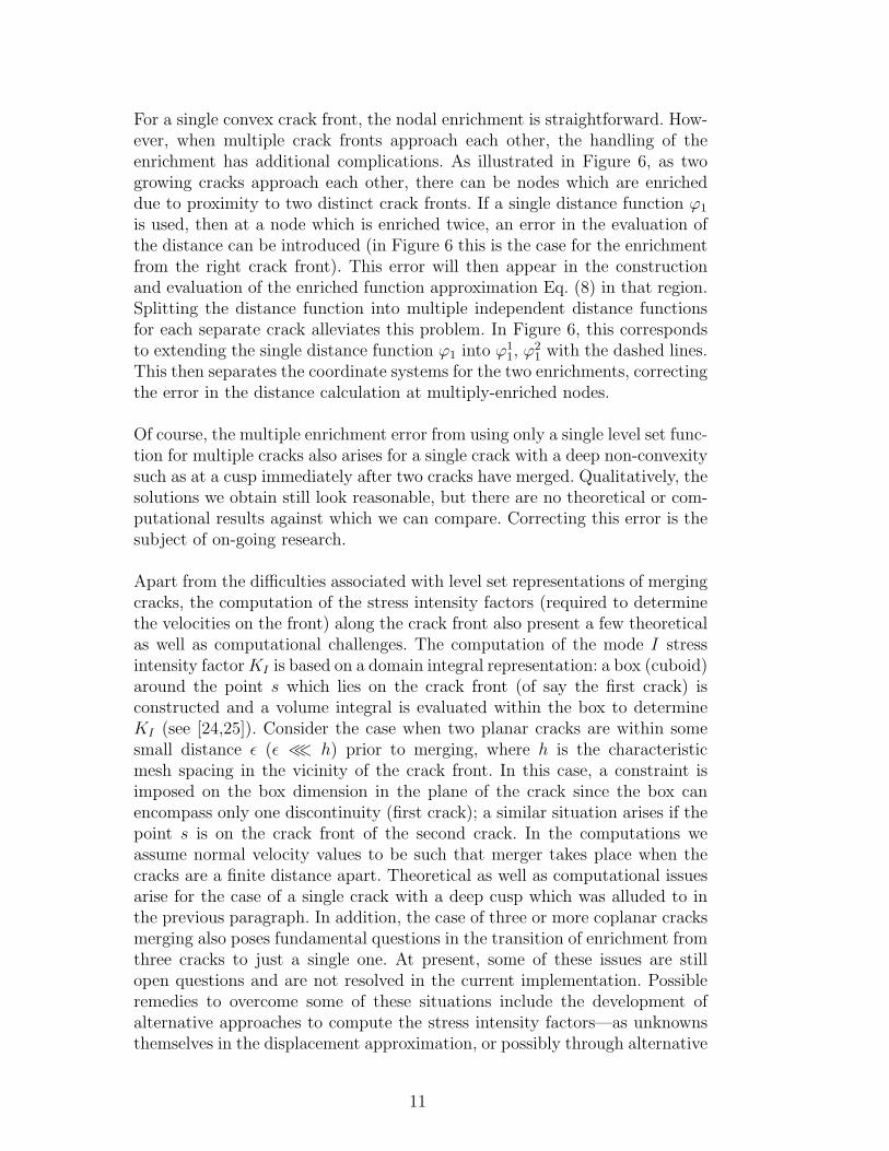
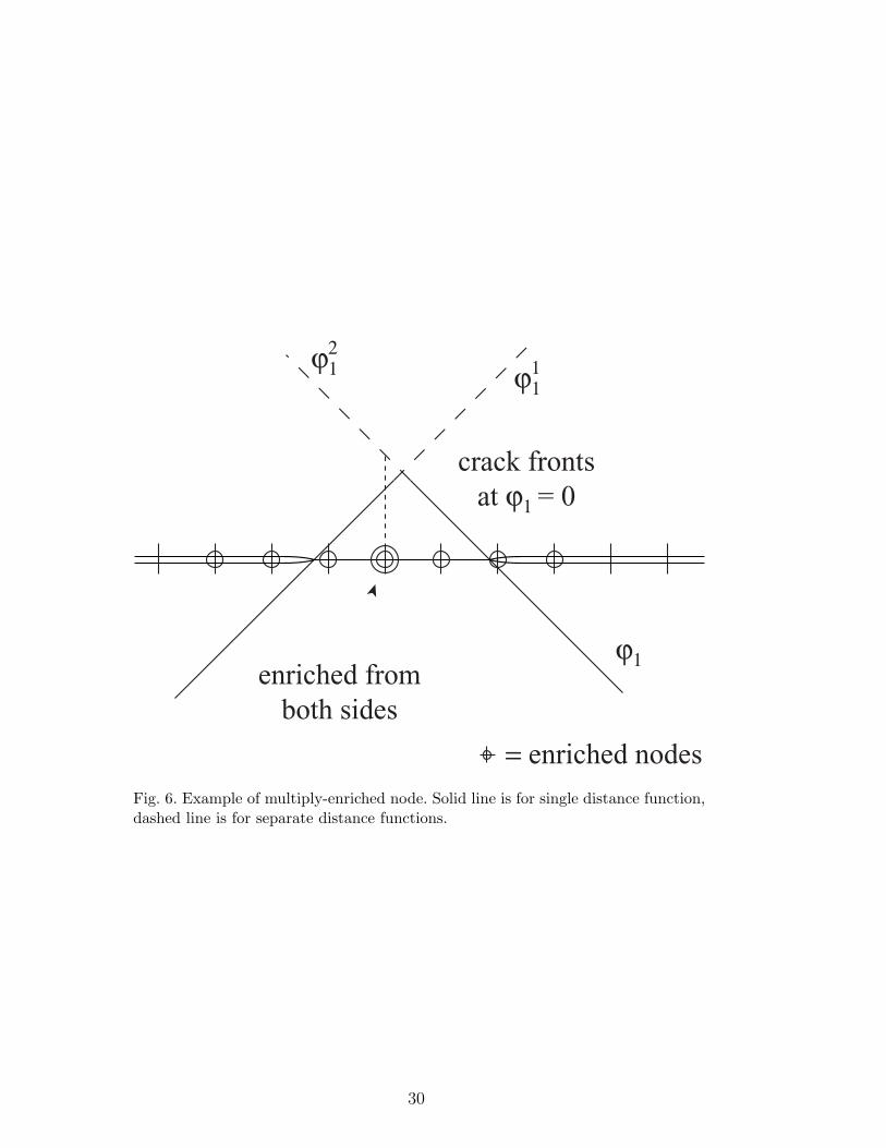
For a single convex crack front, the nodal enrichment is straightforward. How-ever, when multiple crack fronts approach each other, the handling of theenrichment has additional complications. As illustrated in Figure 6, as twogrowing cracks approach each other, there can be nodes which are enricheddue to proximity to two distinct crack fronts. If a single distance function ϕ1

is used, then at a node which is enriched twice, an error in the evaluation ofthe distance can be introduced (in Figure 6 this is the case for the enrichmentfrom the right crack front). This error will then appear in the constructionand evaluation of the enriched function approximation Eq. (8) in that region.Splitting the distance function into multiple independent distance functionsfor each separate crack alleviates this problem. In Figure 6, this correspondsto extending the single distance function ϕ1 into ϕ1

1, ϕ21 with the dashed lines.

This then separates the coordinate systems for the two enrichments, correctingthe error in the distance calculation at multiply-enriched nodes.

Of course, the multiple enrichment error from using only a single level set func-tion for multiple cracks also arises for a single crack with a deep non-convexitysuch as at a cusp immediately after two cracks have merged. Qualitatively, thesolutions we obtain still look reasonable, but there are no theoretical or com-putational results against which we can compare. Correcting this error is thesubject of on-going research.

Apart from the difficulties associated with level set representations of mergingcracks, the computation of the stress intensity factors (required to determinethe velocities on the front) along the crack front also present a few theoreticalas well as computational challenges. The computation of the mode I stressintensity factor KI is based on a domain integral representation: a box (cuboid)around the point s which lies on the crack front (of say the first crack) isconstructed and a volume integral is evaluated within the box to determineKI (see [24,25]). Consider the case when two planar cracks are within somesmall distance ε (ε ≪ h) prior to merging, where h is the characteristicmesh spacing in the vicinity of the crack front. In this case, a constraint isimposed on the box dimension in the plane of the crack since the box canencompass only one discontinuity (first crack); a similar situation arises if thepoint s is on the crack front of the second crack. In the computations weassume normal velocity values to be such that merger takes place when thecracks are a finite distance apart. Theoretical as well as computational issuesarise for the case of a single crack with a deep cusp which was alluded to inthe previous paragraph. In addition, the case of three or more coplanar cracksmerging also poses fundamental questions in the transition of enrichment fromthree cracks to just a single one. At present, some of these issues are stillopen questions and are not resolved in the current implementation. Possibleremedies to overcome some of these situations include the development ofalternative approaches to compute the stress intensity factors—as unknownsthemselves in the displacement approximation, or possibly through alternative

11

techniques to compute the stress intensity factors.

5.4 Crack Growth Algorithm

Fatigue crack growth is assumed to be governed by the Paris law [29]:

da

dN= C(∆K)m, (16)

where C and m are material constants and ∆K is the stress intensity factorrange. For the mode I problems considered here, we use ∆K = KI . Let nbe the number of points on the crack front at which the SIF is evaluated,and ∆amax the maximum user-specified increment normal to the crack front.Then,

∆ai

∆amax

=

(Ki

I

KmaxI

)m

, (17)

which gives the normal growth increment at any point xi ∈ Λc (i = 1, 2, . . . , n).In the computations, for a user-specified n, the crack front is parameterized byarc length s such that st is the total length of the crack front. Then, ds = st/nis used as the increment on the crack front to find the coordinates of the npoints on the crack front. The complete crack growth algorithm now follows:

(1) Step t = 0 (tmax is user-specified). Let ϕ1 be a level set function for thecrack front(s) with ϕ1 = 0 on the crack front(s), ϕ1 < 0 in the crackinterior, and ϕ1 > 0 otherwise. For example, ϕ1 for two ellipses on thex1-x2 plane could be

ϕ1 = min

((x1 − c1)

2

a21

+(x2 − d1)

2

b21

− 1,(x1 − c2)

2

a22

+(x2 − d2)

2

b22

− 1

).

(18)(2) Label each distinct crack using the recursive paint-fill algorithm.(3) Compute the signed distance function(s) ϕi

1 using the FMM with F = 1

in Eq. (3) where ϕi1−1

(0) describes the crack front (zero level set curve)for the ith crack as labelled in step 2. Note that the global signed distancefunction ϕ1 is easily recovered via

ϕ1 = mini

ϕi1. (19)

(4) Evaluate the front speed F at n discrete points on the front(s). Assumingunit time increment in the FMM, we have Fi = ∆ai, where ∆ai arecomputed using Eq. (17).

(5) Given the distance map and a front speed function F defined on thecrack front identified by ϕ−1

1 (0), a speed function Fext can be computed

12

by solving the equation

∇Fext · ∇ϕ1 = 0, (20)

where Fext

∣∣∣ϕ−1

1 (0)= F

∣∣∣ϕ−1

1 (0)using the FMM [1]. The speed function so

constructed is designed so that the speed is constant along lines normalto the crack front.

(6) Once Fext is constructed, it is inserted into Eq. (3) and the FMM is againapplied to compute the crossing time map for the advancing crack front,namely

‖∇ψ‖ =1

Fext

, ψ−1(0) = ϕ1−1(0). (21)

Note that the solution ψ of the above equation is a level set function, butis not a distance map. Now, the advancing crack front location at anytime ∆t later is given by the level curve ψ−1(∆t). The advantage of thistechnique over a standard level set method approach is that an arbitrarilylarge time step ∆t can be taken without introducing instability and themethod is second-order accurate. This is ideal for a problem such as crackpropagation where computation of the speed is very expensive and accu-racy of the distance map ϕ1 is critical to obtaining good approximationsfor the speed.

(7) The FMM is again used to solve

‖∇ϕ1‖ = 1, ϕ1−1(0) = ψ−1(0) (22)

to reconstruct the distance funtion ϕ1.(8) if t < tmax, then increment t (t ← t + 1) and goto step 2.

6 Governing equations

6.1 Strong Form

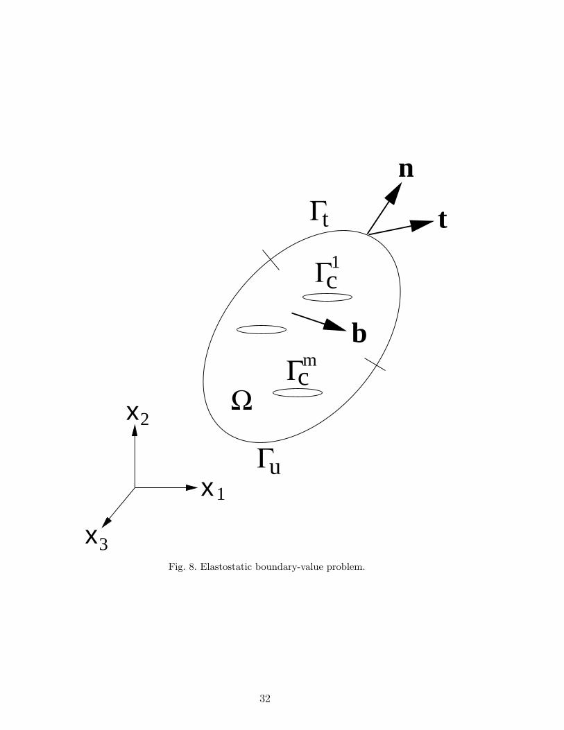
Consider a body Ω ⊂ R3, with boundary Γ (Fig. 8). The boundary Γ consistsof the sets Γu, Γt, and Γi

c, such that Γ = Γu ∪ Γt ∪mi=1 Γi

c. All the internalsurfaces Γi

c are assumed to be traction-free.

The field equations of elastostatics are:

∇ · σ + b = 0 in Ω, (23a)

σ = C : ε, (23b)

ε = ∇su, (23c)

13

where ∇s is the symmetric gradient operator, u is the displacement vector, εis the small strain tensor, σ is the Cauchy stress tensor, b is the body forcevector per unit volume, andC is the tensor of elastic moduli for a homogeneousisotropic material.

The essential and natural boundary conditions are:

u = u on Γu, (24a)

σ · n = t on Γt, (24b)

σ · n = 0 on Γic, (i = 1, 2, . . . , m), (24c)

where n is the unit outward normal to Ω, u and t are prescribed displacementsand tractions, respectively, and m is the number of internal surfaces. Note thatEq. (24c) imposes the condition that the internal surfaces Γi

c be traction-free.

6.2 Weak Form and Discrete Equations

The weak form (principle of virtual work) for linear elastostatics is stated as:Find uh ∈ Vh such that∫

Ωh

σ(uh) : ε(vh) dΩ =∫Ωh

b · vh dΩ +∫Γh

t

t · vh dΓ ∀vh ∈ Vh0 , (25)

where uh(x) ∈ Vh and vh(x) ∈ Vh0 are the approximating trial and test

functions used in the X-FEM. The space Vh is the enriched finite elementspace that satisfy the essential boundary conditions, and which include basisfunctions that are discontinuous across the crack surfaces. The space Vh

0 isthe corresponding space with homogeneous essential boundary conditions.

The trial and test functions, which are based on Eq. (12) are:

uh(x) =∑I

nI∈N

φI(x)uI +∑J

nJ∈Nc

φJ(x)H(x)aJ +∑K

nK∈Nf

φK(x)

(4∑

l=1

ψl(x)blK

),

(26)

vh(x) =∑I

nI∈N

φI(x)vI +∑J

nJ∈Nc

φJ(x)H(x)cJ +∑K

nK∈Nf

φK(x)

(4∑

l=1

ψl(x)elK

),

(27)

where φI(x) are the finite element shape functions, and ψj(x) (j = 1–4) arethe enriched functions for the crack front, which are given in Eq. (8). Onsubstituting the trial and test functions in the weak form given in Eq. (25),

14

and using a standard Galerkin procedure, the discrete linear system Kd = fis obtained. For further details, the interested reader can refer to [40].

7 Numerical Examples

We present fatigue crack propagation simulations of multiple cracks to demon-strate the versatility of the proposed technique. In all problems, numericalintegration is carried out using Gauss-Legendre quadrature. In hexahedralelements associated with only the finite element shape functions, 2 × 2 × 2quadrature is used, and in elements that also have enriched degrees of freedom,6 × 6 × 6 quadrature is used. The elastic constants used in the computationsare: Young’s Modulus E = 105 and Poisson’s ratio ν = 0.3. The finite elementpublic-domain package gmsh [30] is used in the finite element mesh generation.

Fatigue crack growth studies of coplanar cracks are carried out using the Parislaw. The Paris exponent m is assumed to be 3 (m = 2–4 are typical values formetals). Unless otherwise stated, we use a mesh that consists of 24× 24× 24hexahedral elements for all simulations. The mesh spacing in the vicinity ofthe crack front is about five per cent of that near the boundary of the domain(Fig. 4).

For the examples considered in this paper, a 2 × 2 × 2 hexahedral mesh withdomain dimensions of 0.01×0.01×2a is constructed around the crack front tocompute the stress intensity factors (a is the semi-major axis for an ellipticalcrack). The stress intensity factors are computed at n = 18m (see Section 5.4)points on the crack front, where m is the number of initial cracks. For example,for a single penny crack, the normal velocity is evaluated at eighteen (n = 18)points on the crack front, whereas for two elliptical cracks, it is computedat thirty-six (n = 36) points on the crack front of the evolving cracks. TheSIFs on the crack front are required to compute the normal velocity of thefront which is used in the fast marching method to update the signed distancefunctions ϕi

1 (i = 1, . . . ,m), where m is the number of cracks.

7.1 Discretization in the Fast Marching Method

For the fast marching method, we use a 1000×1000 rectilinear grid with bilin-ear interpolation in each grid cell. This might be considered to be prohibitivelyexpensive, however, the efficiency of the FMM means these computations formonly a tiny fraction of the overall simulation time. In return for the more re-fined mesh, it was shown in [39], that on using such a refined grid the SIFswere computed within 10−4 per cent of the values obtained using the exact

15

geometric description. While a less refined mesh could in principle be used,we find the marginal increase in speed to not be worth the potential decreasein accuracy.

7.2 Comparison with Using Mesh-Generation Algorithms

The algorithm presented here is one technique for propagating cracks. An al-ternative approach is to employ traditional finite element-based techniquescoupled with an automatic mesh-generation tool. Today, three-dimensionaltetrahedral mesh generation has reached a fairly sophisticated state of de-velopment. Complex meshes can typically be generated within minutes [2,4].However, in the case of three-dimensional crack modeling, a mesh with gradualchanges in the mesh size is desired, where the mesh size may vary from O(1)on the external boundaries to O(10−4) or less near the crack front in order toobtain accurate stress intensity factors [16]. In this case, adaptive refinementis required with careful control of the aspect ratios of the finite elements: badaspect ratios can lead to poor finite element approximations and loss of accu-racy. Adaptive unstructured meshing algorithms in three dimensions prove tobe more challenging. The mesh generation problem for domains with rapidlyevolving surfaces is still open, and few if any robust algorithms are availableat this time. Such problems are of interest in crash simulation, aeroelasticity,crack propagation, and metal forging applications. For a recent approach inthis direction, see [3].

The approach presented in this paper offers several advantages over automaticmesh generation. In comparison to automatic mesh generation methods, theX-FEM method offers good accuracy on comparatively course meshes. Thismeans there are potential savings in computational cost to achieve the samelevel of accuracy. Also, this method provides greater flexibility for differenttypes of discontinuous fields, making it possible to model cracks in isotropicas well as bimaterial media. Finally, the X-FEM approach can treat multi-ple cracks with arbitrary orientation in three dimensions without any userintervention.

It is difficult to compare the computational cost of the X-FEM method withmesh generation techniques. In the X-FEM method, the mesh generation taskis simpler: the mesh must only conform to the domain, and is generated onlyonce. By comparison, the FEM with mesh generation must regenerate themesh each time step, including both the domain boundary and the internaldiscontinuities such as the crack. On the other hand, for comparable meshes,the X-FEM method will take longer each step due to the increased number ofdegrees of freedom from enrichment. For comparison purposes, the calculationin Fig. 1 required about 30 minutes per time step. In the final analysis, for the

16

single crack, the total computational cost for both methods are comparablefor similar mesh densities [31].

7.3 Fatigue Growth of Coplanar Cracks

Numerical simulations of fatigue crack growth of coplanar multiple cracks arepresented. In order to demonstrate the merging and evolution of multiplecracks, we consider the problem of multiple planar cracks embedded in fullspace under a uniform oscillating (in time) tension σ0

33 = 1. The coordinateaxis x3 is normal to the plane of the crack. Three examples are considered: twopenny-shaped cracks, two elliptical cracks, and three penny-shaped cracks. Inall examples, the numerical model consists of a finite body (bi-unit cube) withthe cracks embedded inside the cube. The crack dimensions are typically atenth or less of the specimen dimensions, and hence finite-specimen effects areminimal initially. Due to crack interactions, there are variations in the SIFsalong the crack fronts. The effect of fatigue is to smooth out these variationsso that after merger and growth, it evolves towards a penny-shape (if oneneglects boundary effects) with a constant KI along the crack front.

7.3.1 Two Penny-Shaped Cracks

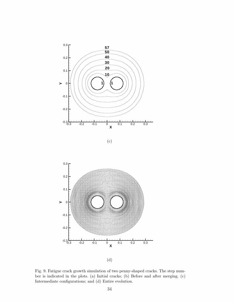
Consider two penny-shaped cracks of radii a = 0.05 that are a distance d =0.05 apart. Unit tractions are specified on the surfaces x3 = ±1. Crack growthsimulations are carried out for 57 steps, and the results for the evolution of thecracks are shown in Fig. 9. The location of the crack fronts before and aftermerger are shown in Fig. 9b, and in addition a few intermediate configurationsare shown in Fig. 9c. As one can observe from Fig. 9d, the crack front shapeis nearly circular after 57 steps.

In order to test the algorithm and the accuracy of the proposed technique, wealso conducted crack growth simulations using an unstructured tetrahedralmesh. The tetrahedral mesh we used is shown in Fig. 10a, which consists of19203 elements; the element size on the boundary is 0.5 and that in the vicinityof the crack front is 0.03 (Fig. 10b). The crack growth simulation results areshown in Figs. 10c and 10d. On comparing the above to the results obtainedusing the hexahedral mesh (Figs. 9b and 9d), we note that both simulationresults are in good agreement. Hence, the results using, both, structured andunstructured meshes are consistent with each other for the evolution of thecrack front.

17

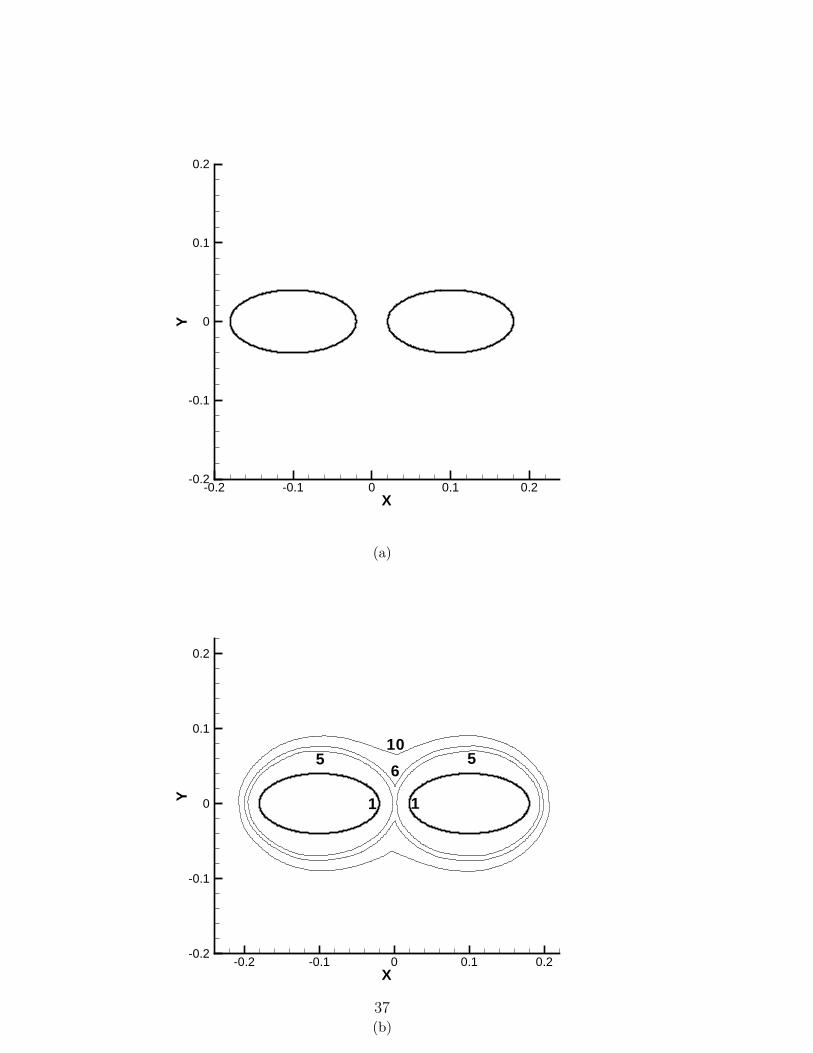
7.3.2 Two Elliptical Cracks

In this example, two elliptical cracks of semi-major and semi-minor axes ofa = 0.08 and b = 0.04, respectively, are considered. The distance between thecracks along the semi-major axis is d = 0.04. Unit tractions are specified on thesurfaces x3 = ±1. The nodal enrichments for the case of a single elliptical crackis shown in Fig. 5 (a = 0.1; b = 0.05). The same mesh is used in this example;however, two cracks lie on the x3 = 0 plane, with only 5–6 finite elementsspanning the major axis of each elliptical crack. The simulation results for theevolution of the cracks under fatigue crack growth is shown in Fig. 11. Thecomputations are carried out for 80 steps. The evolution of the crack frontis plotted in Figs. 11a–11d. The merger of the two crack and the subsequentgrowth of a single crack front is readily handled using the X-FEM/FMMtechnique. In spite of some of the computational difficulties just before themerger (see Section 5.3), the results in Fig. 9 for the growth of two pennycracks as well as the simulations presented in Fig. 11 for elliptical cracks, doindicate that the expected trends are qualitatively captured.

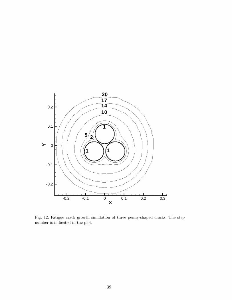
7.3.3 Three Penny-Shaped Cracks

In this example, we consider three penny-shaped cracks of radii a = 0.05(step 1 in Fig. 12). Unit tractions are specified on the surfaces x3 = ±1.The crack growth simulations are carried out for 20 steps, using a maximumincrement that was 30 per cent of the characteristic dimension of the crack(∆amax = 0.0015). The simulation results are shown in Fig. 12, with thezero level set contours indicated at some of the intermediate steps during theevolution. One can observe that the crack front assumes a near circular shapeafter 20 steps. The zero level set contours shown in Fig. 12 are less smooth thanthe simulations presented for the previous two problems. The waviness in thecrack front profile is due to the choice of a larger crack growth increment thanthe earlier examples. A larger ∆amax was used so that the merger of the crackscould occur with a well-defined and single crack front with no disconnectedregions of the crack (ϕ1 < 0) in the interior; such implementational issues wereaddressed in Section 5.3.

8 Conclusions

A numerical technique for modeling fatigue crack propagation of multiplecoplanar cracks was presented. In the proposed method, the Extended Fi-nite Element Method (X-FEM) [40] was coupled to the Fast Marching Method(FMM) [32,33]. In the X-FEM, a discontinuous function and the 2-dimensionalnear-tip displacement fields are added to the finite element approximation to

18

account for the crack using the notion of partition of unity. This enables thedomain to be modeled by finite elements with no explicit meshing of the cracksurfaces. Hence, fatigue crack propagation can be simulated without any user-intervention or the need to remesh as the crack advances.

The level set method is a numerical technique for tracking moving interfaces[28]. The related fast marching method [32] is a computationally attractivealternative for strictly monotonically advancing fronts. In both methods, theevolving interface is represented as a level contour of a function of one higherdimension (i.e., ϕ(x) = C). In the FMM, the motion of the interface is em-bedded in the solution of a static Hamilton-Jacobi equation in terms of ϕ(x).

In a previous study [39], the methodology, algorithm, and implementation forthree-dimensional crack propagation of single cracks was introduced. In thispaper, the algorithms are extended for multiple coplanar cracks. The entirecrack geometry, including one or more cracks, was represented by a singlesigned distance (level set) function ϕ1. To compute the enrichment functionfor distinct cracks, the distance function ϕ1 was split into multiple separatedistance functions, one for each connected crack front. Merging of distinctcracks was handled naturally by the fast marching method with no collisiondetection or mesh reconstruction required. We used the Paris crack growthlaw to advance the crack front.

Numerical simulations of fatigue crack propagation for multiple coplanar penny-shaped and elliptical cracks were presented. The initial characteristic crack-dimensions were much smaller than the specimen dimension so as to minimizefinite-specimen effects. In all simulations, the merging of cracks was easily re-solved and the subsequent growth of a single crack front was observed. Crackgrowth of multiple cracks towards a penny-shape was seen, which is in quali-tative agreement with the theory for embedded cracks in infinite media. Thenumerical technique and simulation results presented in this study point tothe possibility of carrying out automated crack growth simulations of multi-ple cracks in structural components without the need to remesh or maintainthe geometric description of the evolving crack. This is a promising alterna-tive to existing finite element techniques for three-dimensional crack growthmodeling.

The extension of the method presented here to out-of-plane crack growth isalso a subject of further study. A first attempt at such a code has been un-dertaken by Moes et al [23,17]; however, the crack front tracking in this paperwas done using the slower level set method rather than the FMM, requiringa coarser mesh for computing the signed distance function and consequentlyless accurate SIF calculations. Thus, implementing a FMM version for out-of-plane growth coupling the results of this paper with the work in [35] will bethe subject of future research.

19

Acknowledgments

Parts of this work were completed during the summer of 2001, when N.S. wasvisiting the Princeton Materials Institute; the hospitality extended to him byDavid Srolovitz at Princeton University is appreciated.

References

[1] D. Adalsteinsson and J. A. Sethian. The fast construction of extension velocitiesin level set methods. Journal of Computational Physics, 148(1):2–22, 1999.

[2] T. J. Baker. Triangulations, mesh generation and point placement strategies.In D. A. Caughey and M. M. Hafez, editors, Frontiers of Computational FluidDynamics, pages 101–115, New York, NY, 1994. John Wiley & Sons.

[3] T. J. Baker. Mesh movement and metamorphosis. In Proceedings of the 10thInternational Meshing Roundtable, page Available at http://www.imr.sandia.gov/papers/imr10/baker01.ps.gz, Newport Beach, CA, 2001. also to appearin Engineering with Computers (2002).

[4] T. J. Baker and J. C. Vassberg. Tetrahedral mesh generation and optimization.In Proceedings of the 6th International Conference on Numerical GridGeneration, pages 337–349, 1998.

[5] T. Belytschko and T. Black. Elastic crack growth in finite elements with minimalremeshing. International Journal for Numerical Methods in Engineering,45(5):601–620, 1999.

[6] M. Bonnet, G. Maier, and G. Polizzotto. Symmetric Galerkin boundary elementmethod. Applied Mechanics Review, 51:669–704, 1998.

[7] B. J. Carter, P. A. Wawrzynek, and A. R. Ingraffea. Automated 3-dcrack growth simulation. International Journal for Numerical Methods inEngineering, 47:229–253, 2000.

[8] D. L. Chopp. Some improvements of the fast marching method. SIAM Journalon Scientific Computing, 23(1):230–244, 2001.

[9] D. N. Dai, D. A. Hills, and D. Nowell. Modelling of growth of three-dimensionalcracks by a continuous distribution of dislocation loops. ComputationalMechanics, 19:538–544, 1997.

[10] C. Daux, N. Moes, J. Dolbow, N. Sukumar, and T. Belytschko. Arbitrary cracksand holes with the extended finite element method. International Journal forNumerical Methods in Engineering, 48(12):1741–1760, 2000.

[11] G. Dhondt. Automatic 3-D mode I crack propagation calculations withfinite elements. International Journal for Numerical Methods in Engineering,41(4):739–757, 1998.

20

[12] C. A. Duarte, I. Babuska, and J. T. Oden. Generalized finite elementmethods for three dimensional structural mechanics problems. Computers andStructures, 77:215–232, 2000.

[13] C. A. Duarte, O. N. Hamzeh, T. J. Liszka, and W. W Tworzydlo. Theelement partition method for the simulation of three-dimensional dynamiccrack propagation. Computer Methods in Applied Mechanics and Engineering,190(15–17):2227–2262, 2001.

[14] M. Fleming, Y. A. Chu, B. Moran, and T. Belytschko. Enriched element-freeGalerkin methods for crack tip fields. International Journal for NumericalMethods in Engineering, 40:1483–1504, 1997.

[15] W. H. Gerstle, A. R. Ingraffea, and R. Perucchio. Three-dimensional fatiguecrack propagation analysis using the boundary element method. InternationalJournal of Fatigue, 10(3):187–192, 1988.

[16] M. Gosz, J. Dolbow, and B. Moran. Domain integral formulation for stressintensity factor computation along curved three-dimensional interface cracks.International Journal of Solids and Structures, 35:1763–1783, 1998.

[17] A. Gravouil, N. Moes, and T. Belytschko. Non-planar 3D crack growth bythe extended finite element and the level sets – Part II: Level set update.International Journal for Numerical Methods in Engineering, 53(11):2569–2586,2002.

[18] D. A. Hills, P. A. Kelly, D. N. Dai, and A. M. Korsunsky. Solution of CrackProblems: The Distributed Dislocation Technique. Kluwer Academic Publishers,Dordrecht, The Netherlands, 1996.

[19] H. Ji, D. Chopp, and J. E. Dolbow. A hybrid extended finite element/levelset method for modeling phase transformations. International Journal forNumerical Methods in Engineering, 54(8):1209–1233, 2002.

[20] J. M. Melenk and I. Babuska. The partition of unity finite element method:Basic theory and applications. Computer Methods in Applied Mechanics andEngineering, 139:289–314, 1996.

[21] Y. Mi and M. H. Aliabadi. Three-dimensional crack growth simulations usingBEM. Computers and Structures, 52(5):871–878, 1994.

[22] N. Moes, J. Dolbow, and T. Belytschko. A finite element method for crackgrowth without remeshing. International Journal for Numerical Methods inEngineering, 46(1):131–150, 1999.

[23] N. Moes, A. Gravouil, and T. Belytschko. Non-planar 3D crack growth by theextended finite element and level sets. Part I: Mechanical model. InternationalJournal for Numerical Methods in Engineering, 53(11):2549–2568, 2002.

[24] B. Moran and C. F. Shih. Crack tip and associated domain integrals frommomentum and energy balance. Engineering Fracture Mechanics, 27(6):615–641, 1987.

21

[25] G. P. Nikishkov and S. N. Atluri. Calculation of fracture mechanics parametersfor an arbitrary three-dimensional crack by the ‘equivalent domain integralmethod’. International Journal for Numerical Methods in Engineering, 24:1801–1821, 1987.

[26] T. Nishioka and S. N. Atluri. Analytical solution for embedded cracks, and finiteelement alternating method for elliptical surface cracks, subjected to arbitraryloading. Engineering Fracture Mechanics, 17:247–268, 1983.

[27] J. T. Oden, C. A. Duarte, and O. C. Zienkiewicz. A new cloud-based hp finiteelement method. Computer Methods in Applied Mechanics and Engineering,153(1–2):117–126, 1998.

[28] S. Osher and J. A. Sethian. Fronts propagating with curvature-dependent speed:Algorithms based on Hamilton-Jacobi formulations. Journal of ComputationalPhysics, 79(1):12–49, November 1988.

[29] P. C. Paris, M. P. Gomez, and W. E. Anderson. A rationale analytic theory offatigue. The Trend in Engineering, 13(1):9–14, 1961.

[30] J.-F. Remacle and C. Geuzaine. Gmsh finite element grid generator. Availableat http://scorec.rpi.edu/~remacle/Gmsh_Eng.html, 1998.

[31] W. T. Riddell, A. R. Ingraffea, and P. A. Wawrzynek. Experimentalobservations and numerical predictions of three-dimensional fatigue crackpropagation. Engineering Fracture Mechanics, 58(4):293–310, 1997.

[32] J. A. Sethian. A marching level set method for monotonically advancing fronts.Proceedings of the National Academy of Sciences, 93(4):1591–1595, 1996.

[33] J. A. Sethian. Fast marching methods. SIAM Review, 41(2):199–235, 1999.

[34] J. A. Sethian. Level Set Methods & Fast Marching Methods: Evolving Interfacesin Computational Geometry, Fluid Mechanics, Computer Vision, and MaterialsScience. Cambridge University Press, Cambridge, UK, 1999.

[35] M. Stolarska, D. L. Chopp, N. Moes, and T. Belytschko. Modeling crack growthby level sets and the extended finite element method. International Journal forNumerical Methods in Engineering, 51(8):943–960, 2001.

[36] T. Strouboulis, I. Babuska, and K. Copps. The design and analysis of thegeneralized finite element method. Computer Methods in Applied Mechanicsand Engineering, 181(1–3):43–69, 2000.

[37] T. Strouboulis, K. Copps, and I. Babuska. The generalized finite elementmethod. Computer Methods in Applied Mechanics and Engineering, 190(32–33):4081–4193, 2001.

[38] N. Sukumar, D. L. Chopp, N. Moes, and T. Belytschko. Modeling holes andinclusions by level sets in the extended finite element method. ComputerMethods in Applied Mechanics and Engineering, 190(46–47):6183–6200, 2001.

22

[39] N. Sukumar, D. L. Chopp, and B. Moran. Extended finite element methodand fast marching method for three dimensional fatigue crack propagation.Engineering Fracture Mechanics, 70(1):29–48, 2003.

[40] N. Sukumar, N. Moes, B. Moran, and T. Belytschko. Extended finite elementmethod for three-dimensional crack modeling. International Journal forNumerical Methods in Engineering, 48(11):1549–1570, 2000.

[41] K. Vijayakumar and S. N. Atluri. An embedded elliptical flaw in an infinitesolid, subject to arbitrary crack-face tractions. Journal of Applied Mechanics,48:88–96, 1981.

[42] G. Xu and M. Ortiz. A variational boundary integral equation methodfor the analysis of 3d cracks of arbitrary geometry modelled as continuousdistribution of dislocation loops. International Journal for Numerical Methodsin Engineering, 31:3675–3701, 1993.

23

X

Y

Ð0.1 Ð0.05 0 0.05 0.1 0.15

Ð0.1

Ð0.05

0

0.05

0.1

0.15

XÐFEM/FMMExact

Fig. 1. Comparison of penny crack growth to the exact solution.

24

Accepted

Tentative

Distant

ϕ-1(0)

(a)

Accepted

Tentative

Distant

ϕ-1(0)

ϕ-1(t)

ϕ-1(-t)

(b)

Fig. 2. Nodal sets used in the fast marching method. (a) Initial step t = 0; and (b)Intermediate step t > 0.

25

n

θ x

2x

x3

1

Λc

x

*x

r

Crack front

Fig. 3. Coordinate configuration for crack front enrichment functions.

26

Fig. 4. Hexahedral mesh (surface) for the crack growth problems.

27

12

0

(a)

28

4

1

2

3

0

(b)

Fig. 5. Enriched nodes for an elliptical crack. The enriched nodes are indicated byfilled circles and the labels denote the number of nodes enriched in each 4-nodedsurface element. (a) Heaviside function; and (b) Crack-front enrichment function.

29

crack frontsat ϕ1 = 0

ϕ11ϕ1

2

ϕ1

= enriched nodes

enriched fromboth sides

Fig. 6. Example of multiply-enriched node. Solid line is for single distance function,dashed line is for separate distance functions.

30

-3 -2 -1 0 1 2 3-2

0

2

0

0.5

1

1.5

2

2.5

3

3.5

ϕ1

ϕ1−1(0)

1

ϕ12

Fig. 7. Level set distance functions for two coplanar cracks.

31

Γ

ΩΓc

Γ

n

c1

m

t

Γux1

x2

x3

b

t

Fig. 8. Elastostatic boundary-value problem.

32

X

Y

-0.1 -0.05 0 0.05 0.1 0.15

-0.1

-0.05

0

0.05

0.1

(a)

X

Y

-0.15 -0.1 -0.05 0 0.05 0.1 0.15-0.15

-0.1

-0.05

0

0.05

0.1

1 16 6

7

10

(b)

33

X

Y

-0.3 -0.2 -0.1 0 0.1 0.2 0.3-0.3

-0.2

-0.1

0

0.1

0.2

0.3

1

10

1

3020

57

4050

(c)

X

Y

-0.3 -0.2 -0.1 0 0.1 0.2 0.3-0.3

-0.2

-0.1

0

0.1

0.2

0.3

(d)

Fig. 9. Fatigue crack growth simulation of two penny-shaped cracks. The step num-ber is indicated in the plots. (a) Initial cracks; (b) Before and after merging. (c)Intermediate configurations; and (d) Entire evolution.

34

pennycracks

(a)

pennycracks

(b)

35

X

Y

-0.15 -0.1 -0.05 0 0.05 0.1 0.15-0.15

-0.1

-0.05

0

0.05

0.1

11 6 16

7

10

(c)

X

Y

-0.3 -0.2 -0.1 0 0.1 0.2 0.3-0.3

-0.2

-0.1

0

0.1

0.2

0.3

(d)

Fig. 10. Fatigue crack growth simulation of two embedded penny-shaped cracksusing an unstructured mesh. (a) Boundary mesh and cracks; (b) Surface elements inthe vicinity of the cracks; (c) Before and after merger (step numbers are indicated);and (d) Crack evolution (59 steps).

36

X

Y

-0.2 -0.1 0 0.1 0.2-0.2

-0.1

0

0.1

0.2

(a)

X

Y

-0.2 -0.1 0 0.1 0.2-0.2

-0.1

0

0.1

0.2

10

1 1

5 56

(b)37

X

Y

-0.5 -0.4 -0.3 -0.2 -0.1 0 0.1 0.2 0.3 0.4 0.5 0.6

-0.5

-0.4

-0.3

-0.2

-0.1

0

0.1

0.2

0.3

0.4

0.5

20

1 1

3040

10

5060

8070

(c)

X

Y

-0.5 -0.4 -0.3 -0.2 -0.1 0 0.1 0.2 0.3 0.4 0.5-0.5

-0.4

-0.3

-0.2

-0.1

0

0.1

0.2

0.3

0.4

0.5

(d)

Fig. 11. Fatigue crack growth simulation of two embedded elliptical cracks. The stepnumber is indicated in the plots. (a) Initial cracks; (b) Before and after merging.(c) Intermediate configurations; and (d) Entire evolution.

38

X

Y

-0.2 -0.1 0 0.1 0.2 0.3

-0.2

-0.1

0

0.1

0.2

17

1

10

1

25

1

14

20

Fig. 12. Fatigue crack growth simulation of three penny-shaped cracks. The stepnumber is indicated in the plot.

39